Embed Size (px)
Citation preview
SD2006-10-F
Analysis of Maintenance Decision Support System (MDSS) Benefits & Costs
Study SD2006-10
Final Report Prepared by Western Transportation Institute P.O. Box 174250 Bozeman, MT 59717-4250 Iteris, Inc. 1471 Shoreline Drive, Suite 135 Boise, ID 83701-9113 May 2009
MDSS Pooled Fund Study TPF-5(054)

SD2006-10 Page ii Analysis of MDSS Benefits & Costs May 2009
DISCLAIMER The contents of this report, funded in part through grant(s) from the Federal Highway Administration, reflect the views of the authors who are responsible for the facts and accuracy of the data presented herein. The contents do not necessarily reflect the official views or policies of the South Dakota Department of Transportation, the State Transportation Commission, or the Federal Highway Administration. This report does not constitute a standard, specification, or regulation.
ACKNOWLEDGEMENTS This work was performed under the supervision of the SD2006-10 Technical Panel: Phillip Anderle............................. Colorado DOT Jeff Frazier ..................................Wyoming DOT Mike Kisse ............................ North Dakota DOT David Huft ............................ South Dakota DOT Mike Mattison..............................Nebraska DOR
Tony McClellan.............................. Indiana DOT Pamela Mitchell ................New Hampshire DOT Curt Pape ................................... Minnesota DOT Roger Vigdal....................................... Iowa DOT
The work was performed in cooperation with the United States Department of Transportation Federal Highway Administration.
SD2006-10 Page iii Analysis of MDSS Benefits & Costs May 2009
TECHNICAL REPORT STANDARD TITLE PAGE 1. Report No.
SD2006-10-F 2. Government Accession No.
3. Recipient's Catalog No. 5. Report Date
May 12, 2009 4. Title and Subtitle
Analysis of Maintenance Decision Support System (MDSS) Benefits & Costs 6. Performing Organization Code
7. Author(s)
Zhirui Ye, Christopher Strong, Xianming Shi*, and Steven Conger
8. Performing Organization Report No.
10. Work Unit No.
HRZ610(01) 9. Performing Organization Name and Address
Western Transportation Institute P.O. Box 174250, Montana State University Bozeman, MT 59717-4250 (* Principal Investigator) Iteris, Inc. 1471 Shoreline Drive, Suite 135 Boise, ID 83701-9113
11. Contract or Grant No.
310991
13. Type of Report and Period Covered
Final Report October 2006 – May 2009
12. Sponsoring Agency Name and Address
South Dakota Department of Transportation Office of Research 700 East Broadway Avenue Pierre, SD 57501-2586
14. Sponsoring Agency Code
15. Supplementary Notes
An executive summary is published separately as SD2006-10-X. 16. Abstract
This research aimed to assess the benefits and costs associated with implementation of the Pooled fund MDSS by a state transportation agency and to distill this information in a format that is accessible and actionable to transportation agency decision-makers and elected officials. To this end, extensive stakeholder interviews were conducted to help develop the methodology used to analyze MDSS benefits and costs. The research team interviewed two different groups of stakeholders: maintenance personnel at pooled fund member state transportation agencies and selected staff at Meridian Environmental Technologies, the contractor responsible for development of the pooled fund MDSS. A methodology consisting of a baseline data module and a simulation module was developed analyzing tangible benefits, which include reduced material use (agency benefit), improved traffic safety (user benefit), and reduced traffic delay (user benefit). The methodology was applied to three pooled fund states, which belong to different climatologically groups. Analysis results indicated that the use of MDSS could bring more benefits than costs. In addition, a Function Analysis System Technique (FAST) was used to characterize the intangible benefits of MDSS. Finally, a stakeholder outreach plan was developed. Three different formats of outreach materials, Web page, brochure, and PowerPoint presentation, were used to make the results and findings accessible to appropriate audiences. 17. Key Words
Maintenance Decision Support System, benefit cost analysis, traffic safety; traffic delay; winter maintenance
18. Distribution Statement
No restrictions. This document is available to the public from the sponsoring agency.
19. Security Classif. (of this report)
Unclassified 20. Security Classification. (of this page)
Unclassified 21. No. of Pages
143 22. Price

SD2006-10 Page iv Analysis of MDSS Benefits & Costs May 2009
SD2006-10 Page v Analysis of MDSS Benefits & Costs May 2009
TABLE OF CONTENTS DISCLAIMER ........................................................................................................................... ii ACKNOWLEDGEMENTS ....................................................................................................... ii TECHNICAL REPORT STANDARD TITLE PAGE ............................................................. iii TABLE OF CONTENTS........................................................................................................... v LIST OF FIGURES ................................................................................................................ viii LIST OF TABLES .................................................................................................................... ix GLOSSARY OF ACRONYMS................................................................................................. x 1. EXECUTIVE SUMMARY................................................................................................ 1
1.1 Objectives................................................................................................................... 1 1.2 Essential Functions of MDSS .................................................................................... 1 1.3 Research Methodology .............................................................................................. 1 1.4 Research Findings and Conclusions .......................................................................... 3
2. INTRODUCTION ............................................................................................................. 5 2.1 Problem Description .................................................................................................. 5 2.2 Research Objectives ................................................................................................... 6 2.3 Research Scope .......................................................................................................... 6
3. POOLED FUND MDSS .................................................................................................... 8 3.1 MDSS Definition ....................................................................................................... 8 3.2 MDSS History............................................................................................................ 8 3.3 Essential Functions of an MDSS ............................................................................... 9 3.4 Pooled fund MDSS Options..................................................................................... 10 3.5 MDSS Interface........................................................................................................ 11
4. STAKEHOLDER INTERVIEW ..................................................................................... 19 5. METHODOLOGY........................................................................................................... 24
5.1 Definitions................................................................................................................ 24 5.2 MDSS and Winter Maintenance Objectives ............................................................ 25 5.3 Assessing MDSS Benefits ....................................................................................... 26
5.3.1 Use of MDSS as Simulation Tool.................................................................... 26 5.3.2 Identification of Benefits.................................................................................. 27 5.3.3 Risks Affecting Estimation of Benefits............................................................ 29
5.4 Assessing MDSS Costs ............................................................................................ 30 5.4.1 MDSS Vendor Costs ........................................................................................ 30 5.4.2 Weather Forecast Provider Costs ..................................................................... 32 5.4.3 Agency Support Costs...................................................................................... 32
5.5 Benefit-Cost Analysis .............................................................................................. 33 5.5.1 Scope (Step 0) .................................................................................................. 34 5.5.2 Establish Objectives (Step 1) ........................................................................... 35 5.5.3 Identify Constraints and Specify Assumptions (Step 2) .................................. 35 5.5.4 Define Base Case and Identify Alternatives .................................................... 36 5.5.5 Set Analysis Period (Step 4) ............................................................................ 36 5.5.6 Estimate Benefits and Costs Relative to Base Case (Step 7) ........................... 37 5.5.7 Evaluate Risk (Step 8)...................................................................................... 37 5.5.8 Compare Net Benefits and Rank Alternatives ................................................. 38 5.5.9 Make Recommendations.................................................................................. 38
5.6 Summary .................................................................................................................. 38

SD2006-10 Page vi Analysis of MDSS Benefits & Costs May 2009
6. ANALYSIS OF TANGIBLE BENEFITS AND COSTS ................................................ 41 6.1 Storm Identification and Classification.................................................................... 41 6.2 New Hampshire Case Study..................................................................................... 42
6.2.1 Baseline Data ................................................................................................... 43 6.2.2 Simulation Route and Output........................................................................... 44 6.2.3 Benefit-Cost Analysis Results ......................................................................... 45
6.3 Minnesota Case Study.............................................................................................. 47 6.3.1 Baseline Data ................................................................................................... 47 6.3.2 Simulation Route.............................................................................................. 48 6.3.3 Adjustment Factors for Compacted Snow ....................................................... 48 6.3.4 Benefit-Cost Analysis Results ......................................................................... 49
6.4 Colorado Case Study................................................................................................ 51 6.4.1 Baseline Data ................................................................................................... 51 6.4.2 Simulation Route and Material Use ................................................................. 52 6.4.3 Benefit-Cost Analysis Results ......................................................................... 52
6.5 Summary .................................................................................................................. 54 7. ANALYSIS OF INTANGIBLE BENEFITS AND COSTS............................................ 56
7.1 Intangible Benefits and Costs Defined..................................................................... 56 7.2 MDSS Function Analysis......................................................................................... 57 7.3 Intangible Benefits by MDSS Function ................................................................... 59
7.3.1 Portray.............................................................................................................. 59 7.3.2 Predict / Suggest............................................................................................... 60 7.3.3 Integrate ........................................................................................................... 60 7.3.4 Model Pavement Condition ............................................................................. 61 7.3.5 Track Pavement Conditions / Initialize [Model] Conditions ........................... 62 7.3.6 Track Treatments ............................................................................................. 63 7.3.7 Record Resources............................................................................................. 63
7.4 Intangible Benefits from Function Specifications in MDSS.................................... 64 7.4.1 Maintenance Performance Measures ............................................................... 64 7.4.2 Training............................................................................................................ 64 7.4.3 Rules of Practice .............................................................................................. 65
7.5 Intangible Benefits from Essential Supporting Functions Outside MDSS .............. 65 7.5.1 Weather Prediction........................................................................................... 65 7.5.2 Road Patrols / RWIS ........................................................................................ 66 7.5.3 Manual Data Entry / Mobile Data Collection .................................................. 66
7.6 Externality Intangibles ............................................................................................. 67 7.7 Summary .................................................................................................................. 68
8. FINDINGS AND CONCLUSIONS ................................................................................ 70 9. STAKEHOLDER OUTREACH PLAN .......................................................................... 72 10. IMPLEMENTATION RECOMMENDATIONS ........................................................ 73 11. REFERENCES............................................................................................................. 74 Appendix A: Questionnaire for State DOT Stakeholders ........................................................ 77 Appendix B: Questionnaire for Meridian Stakeholders........................................................... 81 Appendix C: Use of MDSS as a Simulator.............................................................................. 84
Simulation System Components .......................................................................................... 84 Weather Information ........................................................................................................ 84 Pavement Model............................................................................................................... 85 MDSS Software Modules ................................................................................................ 86

SD2006-10 Page vii Analysis of MDSS Benefits & Costs May 2009
Simulation Approach ........................................................................................................... 87 Simulation Details................................................................................................................ 89
New Hampshire................................................................................................................ 89 Minnesota......................................................................................................................... 91 Colorado........................................................................................................................... 93
Appendix D: Literature Review on Effects of Weather on Safety, Delay ............................... 96 References .......................................................................................................................... 112
Appendix E: Use of Posted Speed Limits .............................................................................. 115 Appendix F: Calculations of Delay Savings and Safety Benefits.......................................... 117
Delay Benefits.................................................................................................................... 117 Safety Benefits ................................................................................................................... 119 References .......................................................................................................................... 121
Appendix H: Definition of Alternatives................................................................................. 122 Selection of Forecasting Services and Forecast Accuracy................................................. 122 Consistency of Feedback on Actual Maintenance Operations........................................... 123 Use of Treatment Recommendations ................................................................................. 124 Use of In-vehicle Graphical User Interface (GUI)............................................................. 124
Appendix H: Storm Classification ......................................................................................... 126 Appendix I: Weather Station and Availability of Data.......................................................... 129 Appendix J: Determination of Adjustment Factors for Compacted Snow ............................ 131
References .......................................................................................................................... 133

SD2006-10 Page viii Analysis of MDSS Benefits & Costs May 2009
LIST OF FIGURES Figure 1: Benefit-Cost Methodology and Relationship between Level of Service and
Costs........................................................................................................................ 2 Figure 2: MDSS Pooled Fund Study States .............................................................................. 8 Figure 3: Spectrum of Use Levels of MDSS .......................................................................... 10 Figure 4: MDSS GUI Application .......................................................................................... 12 Figure 5: Main Page of the MDSS GUI with Several Page Components Identified .............. 13 Figure 6: Main Page of MDSS GUI in Map View ................................................................. 13 Figure 7: Illustration of the Different Icons that Can Be Clicked within the Map View........ 14 Figure 8: Available Information on the Truck Pop-up Menu. ................................................ 15 Figure 9: Trace Route Function with Application Rate Selected ........................................... 16 Figure 10: Drill-Down Feature for MDSS Routes with Alerts ............................................... 16 Figure 11: Image of All Three Recommendation Options Displayed in the Graph View...... 17 Figure 12: Relationship between LOS and Costs ................................................................... 26 Figure 13: Use of MDSS as a Simulation Tool ...................................................................... 27 Figure 14: Baseline Data Module ........................................................................................... 39 Figure 15: Simulation Module ................................................................................................ 39 Figure 16: Weather Stations in New Hampshire .................................................................... 44 Figure 17: Highway Segment of I-93 in New Hampshire ...................................................... 44 Figure 18: Weather Stations in Minnesota.............................................................................. 48 Figure 19: Highway Segment of I-94 in Minnesota ............................................................... 48 Figure 20: Actual Locations of the MDSS Scenarios ............................................................. 49 Figure 21: Weather Stations in Colorado................................................................................ 52 Figure 22: MDSS Simulation Route I-225 in Colorado ......................................................... 52 Figure 23: FAST Diagram of MDSS Functions ..................................................................... 58 Figure 24: Comparison of Historical Annual Salt Use on NHDOT Maintenance Patrol
M528 with Simulated Salt Use Derived from the MDSS Standard Practice Module .................................................................................................................. 90
Figure 25: Comparison of Historical Annual Salt Use on MnDOT Maintenance Route TP3PR223 with Simulated Salt Use Derived from the MDSS Standard Practice Module .................................................................................................... 92
Figure 26: Comparison of Historical Annual ‘Equivalent Ice Slicer’ Use on CDOT Patrol 20 in the Denver Metro Area with Simulated Salt Use Derived from the MDSS Standard Practice Module ......................................................................... 95
Figure 27: Regression of Severity Index and Safety Adjustment Factors ............................ 132
SD2006-10 Page ix Analysis of MDSS Benefits & Costs May 2009
LIST OF TABLES Table 1: Essential MDSS Functions ......................................................................................... 1 Table 2: Benefit-Cost Summary................................................................................................ 4 Table 3: Essential MDSS Functions ......................................................................................... 9 Table 4: Highway Maintainer (Winter) Needs........................................................................ 10 Table 5: List of Stakeholders Interviewed .............................................................................. 19 Table 6: Number of Respondents by State.............................................................................. 20 Table 7: Summary of State Experience with Pooled Fund MDSS ......................................... 21 Table 8: Assumed MDSS Support Requirements................................................................... 32 Table 9: Taxonomy of MDSS Benefits and Costs .................................................................. 37 Table 10: Cluster Centers........................................................................................................ 42 Table 11: Number of Storm Events in Each Cluster............................................................... 42 Table 12: Durations of Pavement Conditions for Storm Type 1 ............................................ 45 Table 13: MDSS Costs for New Hampshire ........................................................................... 46 Table 14: MDSS Benefits for New Hampshire ...................................................................... 46 Table 15: Material Use in Minnesota...................................................................................... 48 Table 16: MDSS Benefits for Minnesota................................................................................ 49 Table 17: MDSS Costs for Minnesota ................................................................................... 50 Table 18: Material Amounts and Costs in Colorado for Winter 2006-07 .............................. 52 Table 19: MDSS Benefits for Colorado.................................................................................. 53 Table 20: MDSS Costs for Colorado ...................................................................................... 54 Table 21: Summary of Benefit-Cost Analysis ........................................................................ 55 Table 22: Winter Maintenance Goals Taken from Interview Notes and Transcriptions and
Illustrating Their Intangible Nature ...................................................................... 57 Table 23: Intangible Benefit Example .................................................................................... 68 Table 24: Summary of Benefits and Costs.............................................................................. 71 Table 25: Use of Case Study Results ...................................................................................... 73 Table 26: Capabilities of the HiCAPS™ Model Used as the Pavement Model of the PFS
MDSS Modeling System ...................................................................................... 86 Table 27: Delay at Posted Speed Limit & 5 mph Above...................................................... 116 Table 28 : Weather Parameter Values for Classifying Storms ............................................. 128 Table 29: Severity Index of Road Conditions....................................................................... 131 Table 30: Safety Adjustment Factors.................................................................................... 132 Table 31: Speed Adjustment Factors .................................................................................... 132 Table 32: Adjustment Factors for Minnesota Simulation..................................................... 133
SD2006-10 Page x Analysis of MDSS Benefits & Costs May 2009
GLOSSARY OF ACRONYMS AADT Annual Average Daily Traffic ADT Average Daily Traffic ATR Automatic Traffic Recorder DOT Department of Transportation ESS Environmental Sensor Station FAST Function Analysis System Technique FHWA Federal Highway Administration GIS Geographical Information System GUI Graphical User Interface HCI Human Computer Interface MnDOT Minnesota Department of Transportation LOS Level of Service MDC Mobil Data Collection MDSS Maintenance Decision Support System METAR Meteorological Aviation Report NCDC National Climatic Data Center NOAA National Oceanic and Atmospheric Administration NWS National Weather Service PDO Property Damage Only PFS Pooled fund Study RWIS Road Weather Information System STWDSR Surface Transportation Weather Decision Support Requirements

SD2006-10 Page 1 Analysis of MDSS Benefits & Costs May 2009
1. EXECUTIVE SUMMARY
1.1 Objectives The purpose of this research project is to assess the benefits and costs associated with implementation of Maintenance Decision Support System (MDSS) by a state transportation agency, and to distill this information in a format that is accessible and actionable to transportation agency decision-makers and elected officials. The objectives of this project include: describing the essential functions of the Pooled fund MDSS, and characterizing and estimating the benefits and costs of implementing MDSS in state transportation agencies. The results of this assessment are intended for use by South Dakota Department of Transportation (SDDOT) and other pooled fund study MDSS partner agencies in making decisions on future investments in MDSS. This study will also provide a transportation agency with the foundation to evaluate deployment requirements, potential benefits of, and methods for measuring improvements relevant to MDSS technology and philosophy.
1.2 Essential Functions of MDSS The MDSS is a global essential function of itself: it integrates several functions essential to winter maintenance in a single suite, relating them in manners not previously accomplished. These integrated functions are either primary or secondary essential functions. A secondary function is one that is or can be accomplished by existing systems such as road weather information systems (RWIS) or road weather forecasts. Primary functions are those that have been created as part of the MDSS development process such as the road treatment module. The relationship between these functions is shown in Table 1.
Table 1: Essential MDSS Functions
Global In-situ integration of several primary and secondary functions essential to winter maintenance
Primary Secondary Function(s) created as part of MDSS (e.g. road treatment module)
Function(s) accomplished by existing systems (e.g. RWIS, road weather forecasts)
The global essential function of the MDSS is fulfilled as two inter-related applications:
MDSS Application 1: Predict and portray how road conditions will change due to the forecast weather and the application of several candidate road maintenance treatments, based on an assessment of current road and weather conditions and time- and location-specific weather forecasts along transportation routes. (This may be termed a “real-time assessment of current and future conditions”.)
MDSS Application 2: Suggest optimal maintenance treatments that can be achieved within available staffing, equipment, and materials resources. (This may be termed “real-time maintenance recommendations”.)
1.3 Research Methodology The research team conducted extensive interviews with pooled fund stakeholders in order to develop the methodology used to analyze MDSS benefits and costs. The research team interviewed two different groups of stakeholders: maintenance personnel at pooled fund member state transportation
SD2006-10 Page 2 Analysis of MDSS Benefits & Costs May 2009
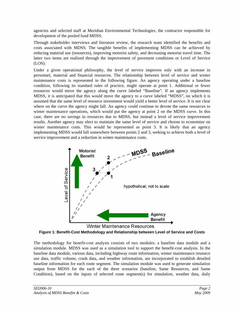
agencies and selected staff at Meridian Environmental Technologies, the contractor responsible for development of the pooled fund MDSS. Through stakeholder interviews and literature review, the research team identified the benefits and costs associated with MDSS. The tangible benefits of implementing MDSS can be achieved by reducing material use (resources), improving motorist safety, and decreasing motorist travel time. The latter two items are realized through the improvement of pavement conditions or Level of Service (LOS). Under a given operational philosophy, the level of service improves only with an increase in personnel, material and financial resources. The relationship between level of service and winter maintenance costs is represented in the following figure. An agency operating under a baseline condition, following its standard rules of practice, might operate at point 1. Additional or fewer resources would move the agency along the curve labeled “Baseline”. If an agency implements MDSS, it is anticipated that this would move the agency to a curve labeled “MDSS”, on which it is assumed that the same level of resource investment would yield a better level of service. It is not clear where on the curve the agency might fall. An agency could continue to devote the same resources to winter maintenance operations, which would put the agency at point 2 on the MDSS curve. In this case, there are no savings in resources due to MDSS, but instead a level of service improvement results. Another agency may elect to maintain the same level of service and choose to economize on winter maintenance costs. This would be represented as point 3. It is likely that an agency implementing MDSS would fall somewhere between points 2 and 3, seeking to achieve both a level of service improvement and a reduction in winter maintenance costs.
Figure 1: Benefit-Cost Methodology and Relationship between Level of Service and Costs
The methodology for benefit-cost analysis consists of two modules: a baseline data module and a simulation module. MDSS was used as a simulation tool to support the benefit-cost analysis. In the baseline data module, various data, including highway route information, winter maintenance resource use data, traffic volume, crash data, and weather information, are incorporated to establish detailed baseline information for each route segment. The simulation module was used to generate simulation output from MDSS for the each of the three scenarios (baseline, Same Resources, and Same Condition), based on the inputs of selected route segment(s) for simulation, weather data, daily

SD2006-10 Page 3 Analysis of MDSS Benefits & Costs May 2009
resource use data, and rules of practice. The simulation outputs from selected route segment(s) are extrapolated to other route segments within the state to achieve a statewide benefit-cost analysis. The research team used a Function Analysis System Technique (FAST) method to analyze the intangible benefits and costs associated with MDSS. A FAST diagram was constructed to assist in understanding the relationship of the functions of the PF-MDSS and identifying intangible benefits of the functions.
1.4 Research Findings and Conclusions This findings and conclusions of this research study include:
1. The exhaustive literature review on weather effects on the roadway system found that, despite numerous studies in this area, there has been wide variance in the quantitative effects of adverse weather. Thus, a synthesis of these effects was presented in this study to help quantify the safety and mobility benefits of deploying MDSS.
2. The stakeholder interviews revealed that the interviewees generally had a positive view of the PF-MDSS. They generally perceived it as a valuable tool for winter maintenance. They believed that MDSS has the potential to help them improve winter maintenance operations, reduce material use, improve scheduling/assignment of personnel, and improve decision making. Respondents from several states also mentioned its potential as an effective training tool. Finally, the level of trust and use of MDSS were anticipated to increase as technical difficulties (communications/computers) were resolved, and as a result, lead to more technological advances in winter maintenance.
3. Through literature review and stakeholder interviews, the research team developed a taxonomy of MDSS benefits and costs. It was perceived that there were three types of benefits and costs associated with the use of MDSS: agency, user (motorists), and society. By using MDSS as a simulator, three benefits including reduced material use (agency benefit) and improved safety and mobility (motorist benefits) were able to be quantified. The methodology for benefit-cost analysis was developed to analyze these tangible benefits and costs.
4. By comparing the actual material use and the simulated use, it was found that they had similar results. This indirectly validates the simulation-based methodology. The analysis method provided the capability of comparing different implementation scenarios and looking at different maintenance results by using rules of practice and MDSS recommendations.
5. Three case studies collectively showed that the benefits of using MDSS outweighed associated costs. The benefit-cost analysis results are presented in the following table. The benefit-cost ratios did not indicate which MDSS scenario was (always) better. However, it is most likely that an agency implementing MDSS would fall somewhere between the Same Resources scenario and the Same Condition scenario, seeking to achieve both a level of service improvement and a reduction in winter maintenance costs. The case studies also showed that there is a trade-off between agency benefits and user benefits. Increased use of material will achieve more motorist benefits while increasing agency costs, and vise versa.

SD2006-10 Page 4 Analysis of MDSS Benefits & Costs May 2009
Table 2: Benefit-Cost Summary
Case State Scenario Benefits User Savings (%) Agency Savings (%) Costs B-C Ratio Same Condition $2,367,409 50 50 7.11
New Hampshire Same Resources $2,884,904 99 1
$332,879 8.67
Same Condition $3,179,828 51 49 6.40 Minnesota
Same Resources $1,369,035 187 -87 $496,952
2.75
Same Condition $3,367,810 49 51 2.25 Colorado
Same Resources $1,985,069 90 10 $1,497,985
1.33
6. The intangible benefits were characterized through identification and analysis of the functions
present in MDSS. Examples of intangible benefits include: Use of the MDSS “forces” a quantitative valuation of performance measures. MDSS provides insight and simulated experience through the training necessary to use it. Outcomes of changes in Rules of Practice can be evaluated through the use of MDSS Successful application of MDSS requires quality weather prediction input. Quality recommendations from MDSS are reliant upon properly sited, appropriately maintained,
and reliable Environmental Sensor Stations (ESS). 7. Intangible benefits can also result from externalities (uncompensated direct impact to non-MDSS
users), including the following: Less tonnage of chemicals used logically lead to reduced impacts on transportation
infrastructure, motor vehicles, and the environment. Use of MDSS suggests a reduction in number of maintenance vehicle round trips to meet the
historical level of service. Use of MDSS will generate more consistent treatment maintenance among maintenance sheds
and result in more seamless road conditions for the road user.

SD2006-10 Page 5 Analysis of MDSS Benefits & Costs May 2009
2. INTRODUCTION
2.1 Problem Description The operators and maintainers of our highway networks are facing increasing demands and consumer expectations for mobility and transportation safety, especially during inclement weather, unprecedented budget and staffing constraints, and growing environmental challenges related to chemical and material use. These forces have provided the impetus to create a new set of tools to assist maintenance managers in meeting these demands in a more efficient manner. This has resulted in a complex and costly operations environment harnessed to the uncertainty of weather forecasting. The new tools address key issues for modern highway maintenance and are often resource-related. These issues include:
funding and staffing constraints experience level of maintenance staff and decision-makers limited equipment availability limited, reliable information with which to make appropriate, timely, and sometimes, critical
decisions inaccurate weather forecasts or ineffective interpretation of those forecasts limited road surface condition information, which can vary dramatically even within short
stretches of highway effectiveness of treatment types on pavement conditions effectiveness of various models
The recent development of the Maintenance Decision Support System (MDSS) has both promised and demonstrated potential answers and solutions to many of these key issues. MDSS uses data fusion to merge state-of-the-art weather forecasting with computerized rules of practice about winter road maintenance. The resulting tool aims to provide maintenance managers with precise surface condition forecasts and treatment recommendations for specific routes (1). The primary suggested benefit of MDSS deployment is the potential to substantially reduce the annual winter maintenance and operations costs of state and local highway agencies through better management of staff and equipment and reduced chemical applications (2). The Federal Highway Administration (FHWA) funded and marshaled collaboration among six national research centers and a pool of maintenance practitioners from several state departments of transportation (DOTs) to develop a functional prototype MDSS. In an effort to practically apply the MDSS concept, a pooled fund study, led by the South Dakota DOT and thirteen other states along with Meridian Environmental Technology, built on this effort by seeking to “build and evaluate an operational and sustainable Maintenance Decision Support System” (3) that “not only satisfies the needs of these states, but also meets or exceeds the present national expectations for a deployed MDSS.” (4) MDSS has evolved from a concept to a field-proven application. However, in a fiscally constrained environment, transportation agencies must have information on how the benefits of applying MDSS for their winter maintenance practices relate to MDSS costs in order to proceed with any decisions on implementation. This study is a careful and substantiated investigation and report of the actual expected expenditures, values, and budgetary models associated with various levels of MDSS deployment, using the pooled fund MDSS as an example. It details anticipated investment, operation and maintenance, sustainability, and institutional advancement. The findings are presented in a manner that will allow

SD2006-10 Page 6 Analysis of MDSS Benefits & Costs May 2009
South Dakota DOT and other pooled fund states to evaluate other commercial MDSS packages. This information will provide a transportation agency with a foundation to evaluate deployment requirements, potential benefits, and methods for measuring improvements relevant to MDSS technology and philosophy.
2.2 Research Objectives The purpose of this research project is to assess the benefits and costs associated with implementation of MDSS by a state transportation agency and to distill this information in a format that is accessible and actionable to transportation agency decision-makers and elected officials. The WTI team understands this end goal and will review existing literature, obtain input from pooled fund study MDSS partners, and use engineering economics techniques to develop estimates of benefits and costs under a variety of practical MDSS implementation alternatives. The RFP subdivides this goal statement into three objectives. First, this project describes the essential functions of a MDSS for winter operations. The essential functions of MDSS (related to its goals) that would be expected in normal winter maintenance operations have been described in reports prepared through the pooled fund study. These functions were discussed in detail with pooled fund study partners and expanded upon in a manner that associates them as components of essential functions. This requires understanding a base case—how an agency performs winter maintenance without MDSS—as well as alternative MDSS implementation scenarios. Second, this research describes the resources needed to supply the essential functions of an MDSS. The description includes technical, financial, operational, maintenance, infrastructure and institutional resources. Gathering this information depended upon intentional stakeholder outreach. Third, this research characterizes and estimates the costs and benefits of deploying MDSS in state transportation departments. As will be discussed later in this report, these benefits and costs comprise a mix of quantifiable and qualitative factors. The results of this assessment are intended for use by SDDOT and other pooled fund study MDSS partner agencies in making decisions on future investments in MDSS. This study will also provide a transportation agency with the foundation to evaluate deployment requirements, potential benefits of, and methods for measuring improvements relevant to MDSS technology and philosophy. Therefore, in addition to undertaking objective, informed research on the effects of MDSS implementation, this project needs to include some effort to develop an outreach approach that ensures that the target audience is identified, contacted, and appropriately informed. By addressing the research objectives in the manner presented above, the research team will provide SDDOT and pooled fund study MDSS partner agencies with a concise and actionable assessment of the potential benefits and costs associated with MDSS implementation.
2.3 Research Scope Nine specific tasks were performed to accomplish the research objectives:
1. Meet with the technical panel to review research work plan, receive suggestions, address concerns, and arrive at a consensus on the project scope of work. This task has been finished through a kickoff meeting with the technical panel.
2. Conduct stakeholder interviews to help develop the analysis methodology and provide supporting information to the study. The interview results are described in Chapter 4.
3. Develop a methodology for benefit-cost analysis. Technical Memo 1 documents the detailed information of the methodology. The description of methodology is presented in Chapter 5 of this final report.

SD2006-10 Page 7 Analysis of MDSS Benefits & Costs May 2009
4. Estimate tangible benefits and costs associated with the deployment and use of the Pooled fund MDSS. Technical Memo 2 will document three case studies of MDSS benefit-cost analysis. The analysis results are also described in Chapter 6 of this report.
5. Characterize Intangible Benefits and Costs. Both Technical Memo 2 and Chapter 7 of this report present the intangible benefits and costs.
6. Document the findings and conclusions from the previous two tasks. The findings and conclusions are presented in Chapter 8 of this report.
7. Distill project findings and recommendations into formats (e.g., Web page, brochure) that are easily accessible to appropriate audience. Chapter 9 of this report briefly describes the formats of outreach materials.
8. Submit a final report that summarizes relevant literature, stakeholder interview results, analysis methodology, case study results, findings and conclusions. This is referred to as this report.
9. Make an executive presentation to the SDDOT Research Review Board summarizing the findings and conclusions. The presentation will be presented to the technical panel members after the submission of the final report.
There were four primary components to the study: stakeholder interviews, methodology development, analysis, and outreach. This report, one of three primary documents resultant from this benefit-cost study, summarizes the project. The other documents comprise two technical reports. The first described the methodology for analyzing the tangible benefits and costs associated with winter use of the MDSS. Technical Memo 2 analyzed the tangible and intangible, benefits and costs associated with the use of MDSS. This study relies on a handful of assumptions. The feasibility of using the selected methodology for analysis depends on MDSS having been validated in its ability to accurately simulate the future pavement condition that will result from weather and maintenance. Through some detailed case studies (5), Meridian has established some confidence that MDSS does reliably predict these pavement conditions. An assumption fundamental to the results presented is that mobile data collection (MDC) is deployed to record the maintenance activities at a spatial and temporal resolution appropriate to integration with the MDSS recommendations and updates.

SD2006-10 Page 8 Analysis of MDSS Benefits & Costs May 2009
3. POOLED FUND MDSS
3.1 MDSS Definition The fundamental principle behind the development of the MDSS is that better information leads to better decisions. MDSS applies this truism specifically to weather information, pavement surface condition, and winter road maintenance decisions. MDSS aims to provide weather and road condition forecasts and real-time treatment recommendations specific to winter road maintenance routes (e.g., treatment locations, types, times, and rates), tailored for winter road maintenance decision makers. With the right information, winter maintenance managers can respond proactively by managing the infrastructure and deploying resources in real-time. Coupled with other advanced technologies, MDSS holds the promise of revolutionizing DOT winter operations. MDSS is an integrated software application that provides users with real-time road treatment guidance for each maintenance route, addressing the fundamental questions of what, how much, and when according to the forecast road weather conditions, the resources available, and local rules of practice. In addition, MDSS can be used as a training tool, as it features a what-if scenario treatment selector that can be used to examine how the road condition might change over a 48-hour period with the user-defined treatment times, chemical types, or application rates.
3.2 MDSS History Two development tracks associated with MDSS are important to consider when defining MDSS. The first development track has been led by the Federal Highway Administration (FHWA). In 2000, FHWA conducted a user needs assessment for surface transportation weather information. As a result, FHWA engaged a pool of maintenance practitioners from several state departments of transportation (DOTs) and researchers from several national laboratories with expertise in weather forecasting and winter road maintenance to develop a prototype winter MDSS. The prototype MDSS was designed and developed to address the end user needs and to facilitate the rapid implementation by the private sector and transportation agencies. FHWA’s functional prototype MDSS capitalized on existing road and weather data sources and the state-of-the-art weather forecasting models and data fusion techniques. A second development track emerged early on when several states realized that the prototype MDSS did not meet their operational needs. This track was supported by FHWA, which intended for states to work with the private sector in developing customized applications to meet their needs. A pooled fund study, led by South Dakota and now also including California, Colorado, Indiana, Iowa, Kansas, Kentucky, Minnesota, Nebraska, New Hampshire, New York, North Dakota, Virginia, and Wyoming, emerged as a natural offshoot of the Federal initiative (see Figure 2). This PFS, initiated in 2002, sought to establish an operational MDSS that meets or exceeds the federal vision of an MDSS (5). The pooled fund states contracted with Meridian Environmental Technology to develop the operational prototype. While the goal of this pooled fund study has been the establishment of an operational MDSS, the project has also been organized as a research project. As such, the MDSS has been in a process of continuous development and improvement based on user recommendations. The pooled fund MDSS has evolved to the point where several member states are deploying it broadly.
Figure 2: MDSS Pooled Fund Study States

SD2006-10 Page 9 Analysis of MDSS Benefits & Costs May 2009
3.3 Essential Functions of an MDSS Whether a product is truly an MDSS or not depends on whether it provides a core set of functions. The essential functions of an MDSS may be visualized in three tiers: global, primary and secondary. The MDSS is a global essential function of itself: it integrates several functions essential to winter maintenance in a single suite, relating them in manners not previously accomplished. These integrated functions are either primary or secondary essential functions. A secondary function is one that is or can be accomplished by existing systems such as road weather information systems (RWIS) or road weather forecasts. Primary functions are those that have been created as part of the MDSS development process such as the road treatment module. The relationship between these functions is shown in Table 3.
Table 3: Essential MDSS Functions
Global In-situ integration of several primary and secondary functions essential to winter maintenance
Primary Secondary Function(s) created as part of MDSS (e.g. road treatment module)
Function(s) accomplished by existing systems (e.g. RWIS, road weather forecasts)
The global essential function of the MDSS is fulfilled as two interrelated applications:
MDSS Application 1: Predict and portray how road conditions will change due to the forecast weather and the application of several candidate road maintenance treatments, based on an assessment of current road and weather conditions and time- and location-specific weather forecasts along transportation routes. (This may be termed a “real-time assessment of current and future conditions”.)
MDSS Application 2: Suggest optimal maintenance treatments that can be achieved within available staffing, equipment, and materials resources. (This may be termed “real-time maintenance recommendations”.)
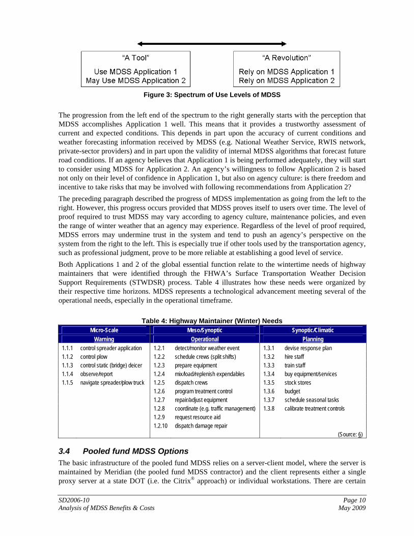
Application 1 serves as a necessary building block for Application 2. Application 1 involves the integration of information on recent and current road and weather conditions, along with reports of winter maintenance actions, from a variety of sources. Application 2 interprets that information and produces recommendations for future action. While the information gathered in Application 1 is useful for making better decisions, Application 2 is where specific courses of action are recommended and MDSS truly becomes a decision-support tool.1 As will be discussed in Chapter 4, the pooled fund states seem to fall on a spectrum of use levels, primarily based on their level of trust in the system. The spectrum may be defined as shown in Figure 3. On the left end of the spectrum are those who view MDSS as a tool. These agencies have shown sufficient interest in MDSS to join the pooled fund and are therefore likely willing to use MDSS at the basic functional level of getting better data on current and forecast conditions, generating treatment recommendations, and comparing alternative treatment scenarios. These agencies may use MDSS for training, but this use may be limited until they have developed confidence in the ability of MDSS to perform the first two functions. On the right end of the spectrum are those who view MDSS as a revolution, in the sense that it changes how winter maintenance operations are done.
1 A third application of MDSS is to archive information from storm events and use them for training of maintenance personnel. This capability also permits post-event analysis of alternative maintenance strategies and different “what-if” analysis of resource allocations or constraints.
SD2006-10 Page 10 Analysis of MDSS Benefits & Costs May 2009
Figure 3: Spectrum of Use Levels of MDSS
The progression from the left end of the spectrum to the right generally starts with the perception that MDSS accomplishes Application 1 well. This means that it provides a trustworthy assessment of current and expected conditions. This depends in part upon the accuracy of current conditions and weather forecasting information received by MDSS (e.g. National Weather Service, RWIS network, private-sector providers) and in part upon the validity of internal MDSS algorithms that forecast future road conditions. If an agency believes that Application 1 is being performed adequately, they will start to consider using MDSS for Application 2. An agency’s willingness to follow Application 2 is based not only on their level of confidence in Application 1, but also on agency culture: is there freedom and incentive to take risks that may be involved with following recommendations from Application 2? The preceding paragraph described the progress of MDSS implementation as going from the left to the right. However, this progress occurs provided that MDSS proves itself to users over time. The level of proof required to trust MDSS may vary according to agency culture, maintenance policies, and even the range of winter weather that an agency may experience. Regardless of the level of proof required, MDSS errors may undermine trust in the system and tend to push an agency’s perspective on the system from the right to the left. This is especially true if other tools used by the transportation agency, such as professional judgment, prove to be more reliable at establishing a good level of service. Both Applications 1 and 2 of the global essential function relate to the wintertime needs of highway maintainers that were identified through the FHWA’s Surface Transportation Weather Decision Support Requirements (STWDSR) process. Table 4 illustrates how these needs were organized by their respective time horizons. MDSS represents a technological advancement meeting several of the operational needs, especially in the operational timeframe.
Table 4: Highway Maintainer (Winter) Needs
Micro-Scale Meso/Synoptic Synoptic/Climatic Warning Operational Planning
1.1.1 control spreader application 1.2.1 detect/monitor weather event 1.3.1 devise response plan 1.1.2 control plow 1.2.2 schedule crews (split shifts) 1.3.2 hire staff 1.1.3 control static (bridge) deicer 1.2.3 prepare equipment 1.3.3 train staff 1.1.4 observe/report 1.2.4 mix/load/replenish expendables 1.3.4 buy equipment/services 1.1.5 navigate spreader/plow truck 1.2.5 dispatch crews 1.3.5 stock stores 1.2.6 program treatment control 1.3.6 budget 1.2.7 repair/adjust equipment 1.3.7 schedule seasonal tasks 1.2.8 coordinate (e.g. traffic management) 1.3.8 calibrate treatment controls 1.2.9 request resource aid 1.2.10 dispatch damage repair (Source: 6)
3.4 Pooled fund MDSS Options The basic infrastructure of the pooled fund MDSS relies on a server-client model, where the server is maintained by Meridian (the pooled fund MDSS contractor) and the client represents either a single proxy server at a state DOT (i.e. the Citrix® approach) or individual workstations. There are certain
SD2006-10 Page 11 Analysis of MDSS Benefits & Costs May 2009
requirements, such as bandwidth and processor speed, on the client side but the system has been designed to not require significant additional computer hardware investment by the DOT. There are a variety of ways in which a transportation agency may choose to implement the pooled fund MDSS. A few are directly relevant to the development of this benefit-cost analysis and are discussed in this section.
Forecasting Services. The pooled fund MDSS currently uses forecasts created by Meridian, but the software has been designed to accept forecast input from other sources. The vision that has emerged from the pooled fund MDSS is that an agency could enter into two procurement arrangements: one in relation to MDSS acquisition and support, and a second in relation to provision of weather forecasting inputs for MDSS. While both services may be furnished by the same vendor, this is not essential.
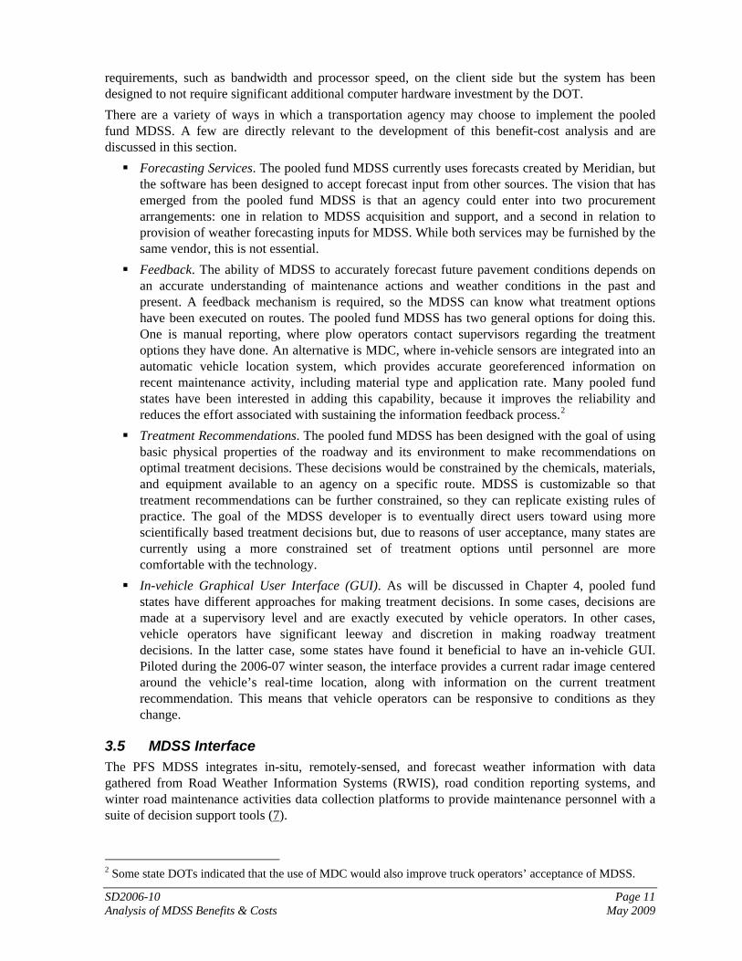
Feedback. The ability of MDSS to accurately forecast future pavement conditions depends on an accurate understanding of maintenance actions and weather conditions in the past and present. A feedback mechanism is required, so the MDSS can know what treatment options have been executed on routes. The pooled fund MDSS has two general options for doing this. One is manual reporting, where plow operators contact supervisors regarding the treatment options they have done. An alternative is MDC, where in-vehicle sensors are integrated into an automatic vehicle location system, which provides accurate georeferenced information on recent maintenance activity, including material type and application rate. Many pooled fund states have been interested in adding this capability, because it improves the reliability and reduces the effort associated with sustaining the information feedback process.2
Treatment Recommendations. The pooled fund MDSS has been designed with the goal of using basic physical properties of the roadway and its environment to make recommendations on optimal treatment decisions. These decisions would be constrained by the chemicals, materials, and equipment available to an agency on a specific route. MDSS is customizable so that treatment recommendations can be further constrained, so they can replicate existing rules of practice. The goal of the MDSS developer is to eventually direct users toward using more scientifically based treatment decisions but, due to reasons of user acceptance, many states are currently using a more constrained set of treatment options until personnel are more comfortable with the technology.
In-vehicle Graphical User Interface (GUI). As will be discussed in Chapter 4, pooled fund states have different approaches for making treatment decisions. In some cases, decisions are made at a supervisory level and are exactly executed by vehicle operators. In other cases, vehicle operators have significant leeway and discretion in making roadway treatment decisions. In the latter case, some states have found it beneficial to have an in-vehicle GUI. Piloted during the 2006-07 winter season, the interface provides a current radar image centered around the vehicle’s real-time location, along with information on the current treatment recommendation. This means that vehicle operators can be responsive to conditions as they change.
3.5 MDSS Interface The PFS MDSS integrates in-situ, remotely-sensed, and forecast weather information with data gathered from Road Weather Information Systems (RWIS), road condition reporting systems, and winter road maintenance activities data collection platforms to provide maintenance personnel with a suite of decision support tools (7).
2 Some state DOTs indicated that the use of MDC would also improve truck operators’ acceptance of MDSS.

SD2006-10 Page 12 Analysis of MDSS Benefits & Costs May 2009
The user interface for the PFS MDSS is a client-side GUI, intended for download and installation on individual user’s machines or on Citrix® servers accessed by many users. The Primary Panel of the MDSS GUI holds most of the functionality of the PFS MDSS from the user’s perspective. The Primary Panel can host one of four different views. These views are the Map View, Route View, RWIS View, and METAR (Meteorological Aviation Report) View. The user selects which view is active in the Primary Panel by either using selection tools in the Support Panel, or, by simply clicking on one of many objects located on the map display (when already in Map View), and selecting ‘Switch View’ from the object’s pop-up menu.
The MDSS GUI (Figure 4) supports a wide variety of features to focus on issues that impact the evolution of the road surface, not only due to weather, but also due to traffic, maintenance operations, and other critical factors. The MDSS focuses specifically on maintenance issues, and its components serve as tools to assist the decision maker with planning and operations issues related directly to snow and ice removal. It is based upon a three-panel layout (Figure 5). The upper-left panel is called the Alert Panel, the lower-left panel is called the Support Panel, and the main body of the display, which carries most of the functionality of the MDSS, is called the Primary Panel. Several different data views may be displayed in the Primary Panel, but the Alert and Support Panels always remain visible. In order to function well in all environments, the client application has been designed to work with a minimum 600x800 screen resolution, but can easily be maximized to take advantage of additional screen dimensions when available.
Figure 4: MDSS GUI Application
Map View is the main screen displayed when the MDSS starts. The displayed region and overlays are configured by the user.

SD2006-10 Page 13 Analysis of MDSS Benefits & Costs May 2009
MMeennuu BBaarr
DDyynnaammiicc OOvveerrllaayyss
CCoonnttrrooll BBuuttttoonnss,,
DDaattaa IIccoonnss && S ii
AAlleerrtt PPaanneell
SSuuppppoorrtt PPaanneell
TTiimmee CCoonnttrrooll
Figure 5: Main Page of the MDSS GUI with Several Page Components Identified
Figure 6: Main Page of MDSS GUI in Map View

SD2006-10 Page 14 Analysis of MDSS Benefits & Costs May 2009
The Map View (Figure 6) is the geospatial display component of the MDSS GUI. It is the default view seen when the application is launched. Users are provided a base map with pan, zoom, and static Geographical Information System (GIS) overlay capabilities (e.g., counties, cities, roads, etc.). In addition, the MDSS GUI presently supports four dynamic overlay types: MDSS Routes, Background, METAR, and RWIS. These overlays are dynamic in the sense that they display data that changes over time. The user is provided a time slider that can be moved forward or backward to view past, present, or future data in a geospatial format. Customization and configuration tools are also provided such that users may pre-select common combinations of Map Views and static overlays, as well as combinations of dynamic data. This allows a user to set up several one-click functions that permit quick and efficient investigation of data when time is at a premium. One of the key features of the MDSS GUI is the interactive map feature, referred to as drill-down capability. Every data icon (truck and camera), most dynamic overlays (METAR observation, RWIS observation, or MDSS Route), the METAR and RWIS location static overlays, and the routes or counties relating to alerts in the alert panel, can be clicked to receive further data about the point at the selected time. A user can left-click on any of these icons to receive more information regarding the variable displayed. In most cases, the information will be an extension of the information available from the icon at the selected time. For example, while the METAR and RWIS air temperatures are being displayed, clicking on one of the observations will cause all variables for that time at that location to be displayed in a pop-up window. The procedure is the same whether looking at current data, past data, or future data (where available). Clicking on the item will display more information for that point at the selected time. For alert information, however, clicking on a route (or county, for National Weather Service - NWS alerts) will display details about all alerts for all times for that route (or county).
MDSS Route
RWIS Icon
Truck Icon
Camera Icon
METAR Icon
MDSS Route
RWIS Icon
Truck Icon
Camera Icon
METAR Icon
Figure 7: Illustration of the Different Icons that Can Be Clicked within the Map View
SD2006-10 Page 15 Analysis of MDSS Benefits & Costs May 2009
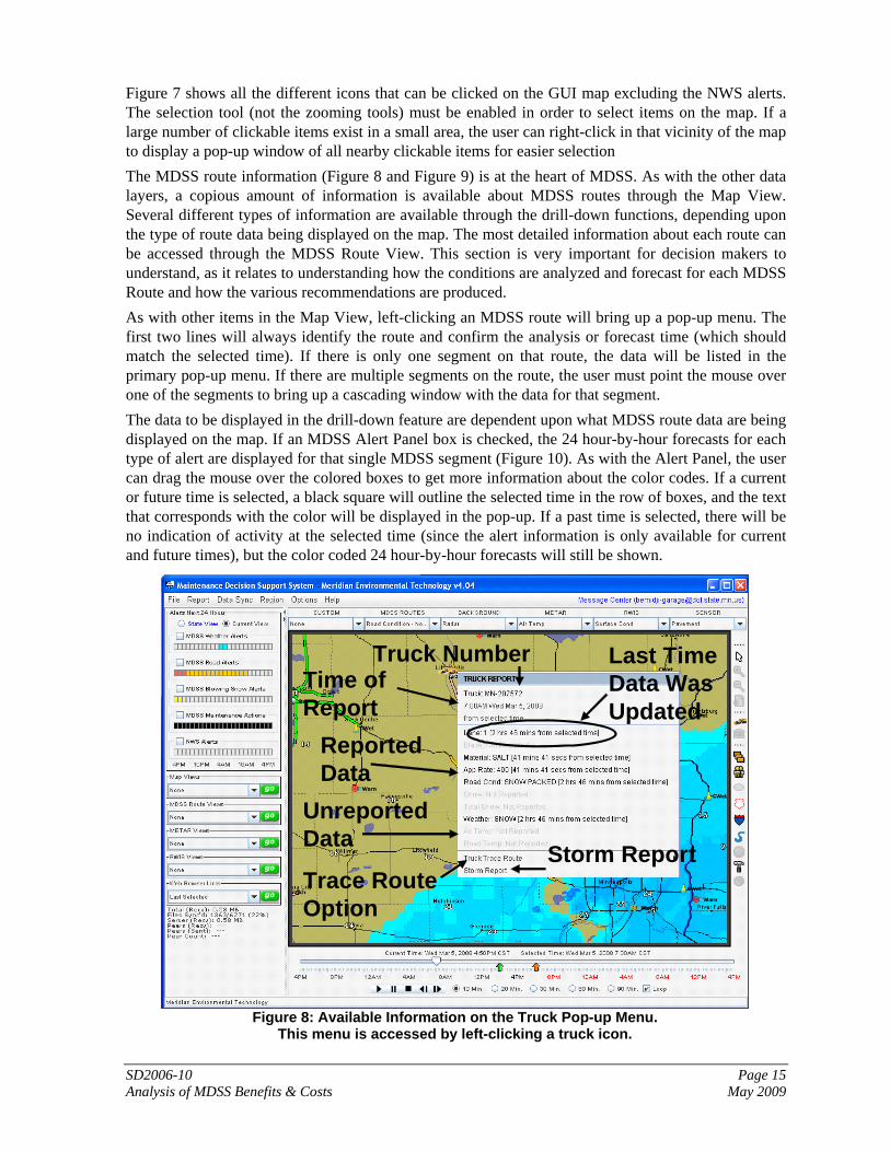
Figure 7 shows all the different icons that can be clicked on the GUI map excluding the NWS alerts. The selection tool (not the zooming tools) must be enabled in order to select items on the map. If a large number of clickable items exist in a small area, the user can right-click in that vicinity of the map to display a pop-up window of all nearby clickable items for easier selection The MDSS route information (Figure 8 and Figure 9) is at the heart of MDSS. As with the other data layers, a copious amount of information is available about MDSS routes through the Map View. Several different types of information are available through the drill-down functions, depending upon the type of route data being displayed on the map. The most detailed information about each route can be accessed through the MDSS Route View. This section is very important for decision makers to understand, as it relates to understanding how the conditions are analyzed and forecast for each MDSS Route and how the various recommendations are produced. As with other items in the Map View, left-clicking an MDSS route will bring up a pop-up menu. The first two lines will always identify the route and confirm the analysis or forecast time (which should match the selected time). If there is only one segment on that route, the data will be listed in the primary pop-up menu. If there are multiple segments on the route, the user must point the mouse over one of the segments to bring up a cascading window with the data for that segment. The data to be displayed in the drill-down feature are dependent upon what MDSS route data are being displayed on the map. If an MDSS Alert Panel box is checked, the 24 hour-by-hour forecasts for each type of alert are displayed for that single MDSS segment (Figure 10). As with the Alert Panel, the user can drag the mouse over the colored boxes to get more information about the color codes. If a current or future time is selected, a black square will outline the selected time in the row of boxes, and the text that corresponds with the color will be displayed in the pop-up. If a past time is selected, there will be no indication of activity at the selected time (since the alert information is only available for current and future times), but the color coded 24 hour-by-hour forecasts will still be shown.
Storm ReportTrace RouteOption
Last Time Data Was Updated
Truck NumberTime of Report
Reported Data
Unreported Data
Figure 8: Available Information on the Truck Pop-up Menu.
This menu is accessed by left-clicking a truck icon.

SD2006-10 Page 16 Analysis of MDSS Benefits & Costs May 2009
Clickable dots represent previous Truck locations
Figure 9: Trace Route Function with Application Rate Selected
The function allows a user to see previous locations, maintenance actions, and other reports for a particular truck.
Current Time Selected
Figure 10: Drill-Down Feature for MDSS Routes with Alerts

SD2006-10 Page 17 Analysis of MDSS Benefits & Costs May 2009
As noted in Figure 11, three recommendation options can be displayed in the MDSS Route View. The user may check one, two, or all three (but never zero) to see the pavement and maintenance related variables that are based upon the given treatment option(s). The options are color-coded to make viewing in the tables and graphs easier. The purple label corresponds to the ‘None/Alternative’ option, which by default assumes no further maintenance action(s) will be conducted on the road. If a ‘What-If’ scenario (described later) has been established, then this color becomes the ‘Alternative’ option based upon that selected practice. The green label corresponds to the ‘MDSS Recommended’ option, which is based upon the recommendation(s) generated scientifically by the pavement model, bounded by the operational restraints imposed by the user(s) or agency during the configuration of the MDSS route. The restraints are generally technical in nature (e.g. hours of operation, available maintenance chemicals, minimum and maximum application rates due to political, mechanical, environmental, or geographical limitations, etc.), but are generally wide enough to permit the MDSS to ‘flex its muscle’ in making the most scientifically sound recommendation for the situation.
The pink label corresponds to the ‘Standard’ option, which is based upon the rules of practice approach to winter road maintenance. These recommendations are arrived at via a flow chart or cookbook provided by the agency or generically provided by the Federal Highway Administration (FHWA) rules of practice. They are based solely on predetermined reactions to a given road and weather forecast, without regard to the reaction of the pavement model to that specific scenario. Despite this limitation, the rules are based upon a long history of situational observations, and can be
Three graphs for one variable(Maintenance Action)
Figure 11: Image of All Three Recommendation Options Displayed in the Graph View Note that the highlighted variable (maintenance action) indicates no actions for the
purple ‘None/Alternative’ selection, one action recommended by ‘MDSS’, and several actions in the ‘Standard’ response. The three graphs above this section
indicate a period of slushy roads in response to the Standard recommended actions; immediate dry roads in response to the MDSS recommended action, and a long
period of icy roads in reaction to taking no action.

SD2006-10 Page 18 Analysis of MDSS Benefits & Costs May 2009
very good, particularly in a strategic situation. In a tactical setting, however, this lack of flexibility can result in inconsistent recommendations for the real-world scenario. For each recommendation option that is checked, there is a separate version of each pavement or maintenance related variable in the graphs or tables. In the graph view, the items for different recommendations are generally grouped, when possible, in the same graph for comparison. As with the three options in the Map View, note there is no difference in these variables for past times, as these are based upon observations, analyses, and reports. The only differences will be at forecast times, as not only will the maintenance recommendations differ at times but, more importantly, so will the pavement temperature and condition as the dynamic layer (the layer of water, snow, ice, chemicals, etc. atop the pavement surface) evolves in very different manners based upon different treatment strategies.

SD2006-10 Page 19 Analysis of MDSS Benefits & Costs May 2009
4. STAKEHOLDER INTERVIEW In 2007, the research team conducted extensive interviews with pooled fund stakeholders in order to develop the methodology used to analyze MDSS benefits and costs. The research team interviewed two different groups of stakeholders: maintenance personnel at pooled fund member state transportation agencies and selected staff at Meridian Environmental Technologies, the contractor responsible for development of the pooled fund MDSS. At a high level, the research team sought to understand the following:
What are the objectives of winter maintenance operations and how might these objectives be supported by MDSS?
What are the potential benefits and costs (tangible and intangible) associated with MDSS and how would they be assessed?
What would be a logical base case against which MDSS implementation could be assessed? What data would be needed to support quantitative analysis of benefits and costs of MDSS? What are likely use cases, in terms of extent and level of functionality?
Since they have paid for costs associated with MDSS implementation, pooled fund member states are necessarily the primary focus of the benefit-cost analysis3. The research team sought to interview a cross-section of stakeholders with MDSS familiarity in each state, in order to better capture the perceived value and challenges of MDSS. Table 5 lists the names of individuals who were interviewed by telephone for each state.
Table 5: List of Stakeholders Interviewed State Persons State Persons State Persons
Colorado Wayne Lupton Minnesota Curt Pape South Dakota Ray McLaughlin Phillip Anderle Nolan Kloehn Larry Kirschenman Rick Jensen Daniel Leister John Forman D’Waye Gaymon New Hampshire Mark Hemmelein Greg Fuller Indiana Dennis Belter Pamela Mitchell Darin Bergquist Tony McClellan Frank Qualey Ed Rodgers John McIntire North Dakota Mike Kisse Wyoming Don Bridges Gary Phillips Dickerson District Jeff Frazier Mike Rivers
John, Aaron, Peter Sailor, Kevin Kaily Tim McGary
Iowa Ed Mahoney Grand Forks District Dale, Paul, Ron Rich Hedlund Fargo District Bruce, Steve, Jerry Jim Vansickle Roger Vigdal
Note: California was not interviewed during the stakeholder interviews as they were new to the pooled fund study.
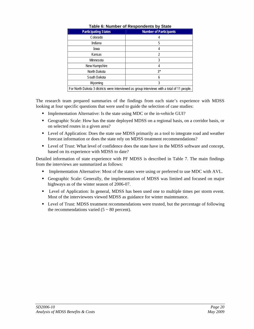
The questionnaire used for interviewing stakeholders from member states is included as Appendix B. Table 6 shows the number of participants in MDSS interviews for each of nine pooled fund states.
3 The interview with Meridian stakeholders was used to flesh out the research team’s understanding of MDSS. Questions used in interviewing Meridian personnel are included in Appendix C. The results of these interviews are not included in this document.
SD2006-10 Page 20 Analysis of MDSS Benefits & Costs May 2009
Table 6: Number of Respondents by State Participating States Number of Participants
Colorado 4 Indiana 5
Iowa 4 Kansas 2
Minnesota 3 New Hampshire 4
North Dakota 3* South Dakota 6
Wyoming 3 For North Dakota 3 districts were interviewed as group interviews with a total of 11 people.
The research team prepared summaries of the findings from each state’s experience with MDSS looking at four specific questions that were used to guide the selection of case studies:
Implementation Alternative: Is the state using MDC or the in-vehicle GUI? Geographic Scale: How has the state deployed MDSS on a regional basis, on a corridor basis, or
on selected routes in a given area? Level of Application: Does the state use MDSS primarily as a tool to integrate road and weather
forecast information or does the state rely on MDSS treatment recommendations? Level of Trust: What level of confidence does the state have in the MDSS software and concept,
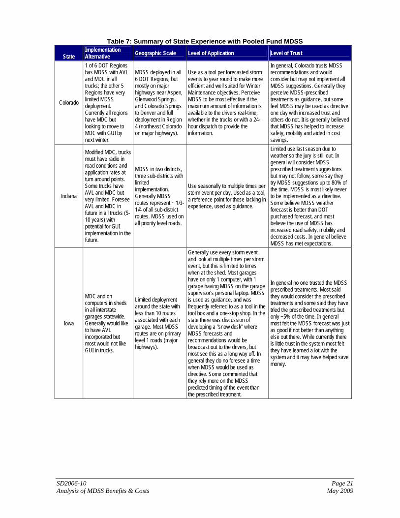
based on its experience with MDSS to date? Detailed information of state experience with PF MDSS is described in Table 7. The main findings from the interviews are summarized as follows:
Implementation Alternative: Most of the states were using or preferred to use MDC with AVL. Geographic Scale: Generally, the implementation of MDSS was limited and focused on major
highways as of the winter season of 2006-07. Level of Application: In general, MDSS has been used one to multiple times per storm event.
Most of the interviewees viewed MDSS as guidance for winter maintenance. Level of Trust: MDSS treatment recommendations were trusted, but the percentage of following
the recommendations varied (5 ~ 80 percent).
SD2006-10 Page 21 Analysis of MDSS Benefits & Costs May 2009
Table 7: Summary of State Experience with Pooled Fund MDSS
State Implementation Alternative Geographic Scale Level of Application Level of Trust
Colorado
1 of 6 DOT Regions has MDSS with AVL and MDC in all trucks; the other 5 Regions have very limited MDSS deployment. Currently all regions have MDC but looking to move to MDC with GUI by next winter.
MDSS deployed in all 6 DOT Regions, but mostly on major highways near Aspen, Glenwood Springs, and Colorado Springs to Denver and full deployment in Region 4 (northeast Colorado on major highways).
Use as a tool per forecasted storm events to year round to make more efficient and well suited for Winter Maintenance objectives. Perceive MDSS to be most effective if the maximum amount of information is available to the drivers real-time, whether in the trucks or with a 24-hour dispatch to provide the information.
In general, Colorado trusts MDSS recommendations and would consider but may not implement all MDSS suggestions. Generally they perceive MDSS-prescribed treatments as guidance, but some feel MDSS may be used as directive one day with increased trust and others do not. It is generally believed that MDSS has helped to increase safety, mobility and aided in cost savings.
Indiana
Modified MDC, trucks must have radio in road conditions and application rates at turn around points. Some trucks have AVL and MDC but very limited. Foresee AVL and MDC in future in all trucks (5-10 years) with potential for GUI implementation in the future.
MDSS in two districts, three sub-districts with limited implementation. Generally MDSS routes represent ~ 1/3-1/4 of all sub-district routes. MDSS used on all priority level roads.
Use seasonally to multiple times per storm event per day. Used as a tool, a reference point for those lacking in experience, used as guidance.
Limited use last season due to weather so the jury is still out. In general will consider MDSS prescribed treatment suggestions but may not follow, some say they try MDSS suggestions up to 80% of the time. MDSS is most likely never to be implemented as a directive. Some believe MDSS weather forecast is better than DOT purchased forecast, and most believe the use of MDSS has increased road safety, mobility and decreased costs. In general believe MDSS has met expectations.
Iowa
MDC and on computers in sheds in all interstate garages statewide. Generally would like to have AVL incorporated but most would not like GUI in trucks.
Limited deployment around the state with less than 10 routes associated with each garage. Most MDSS routes are on primary level 1 roads (major highways).
Generally use every storm event and look at multiple times per storm event, but this is limited to times when at the shed. Most garages have on only 1 computer, with 1 garage having MDSS on the garage supervisor’s personal laptop. MDSS is used as guidance, and was frequently referred to as a tool in the tool box and a one-stop shop. In the state there was discussion of developing a “snow desk” where MDSS forecasts and recommendations would be broadcast out to the drivers, but most see this as a long way off. In general they do no foresee a time when MDSS would be used as directive. Some commented that they rely more on the MDSS predicted timing of the event than the prescribed treatment.
In general no one trusted the MDSS prescribed treatments. Most said they would consider the prescribed treatments and some said they have tried the prescribed treatments but only ~5% of the time. In general most felt the MDSS forecast was just as good if not better than anything else out there. While currently there is little trust in the system most felt they have learned a lot with the system and it may have helped save money.
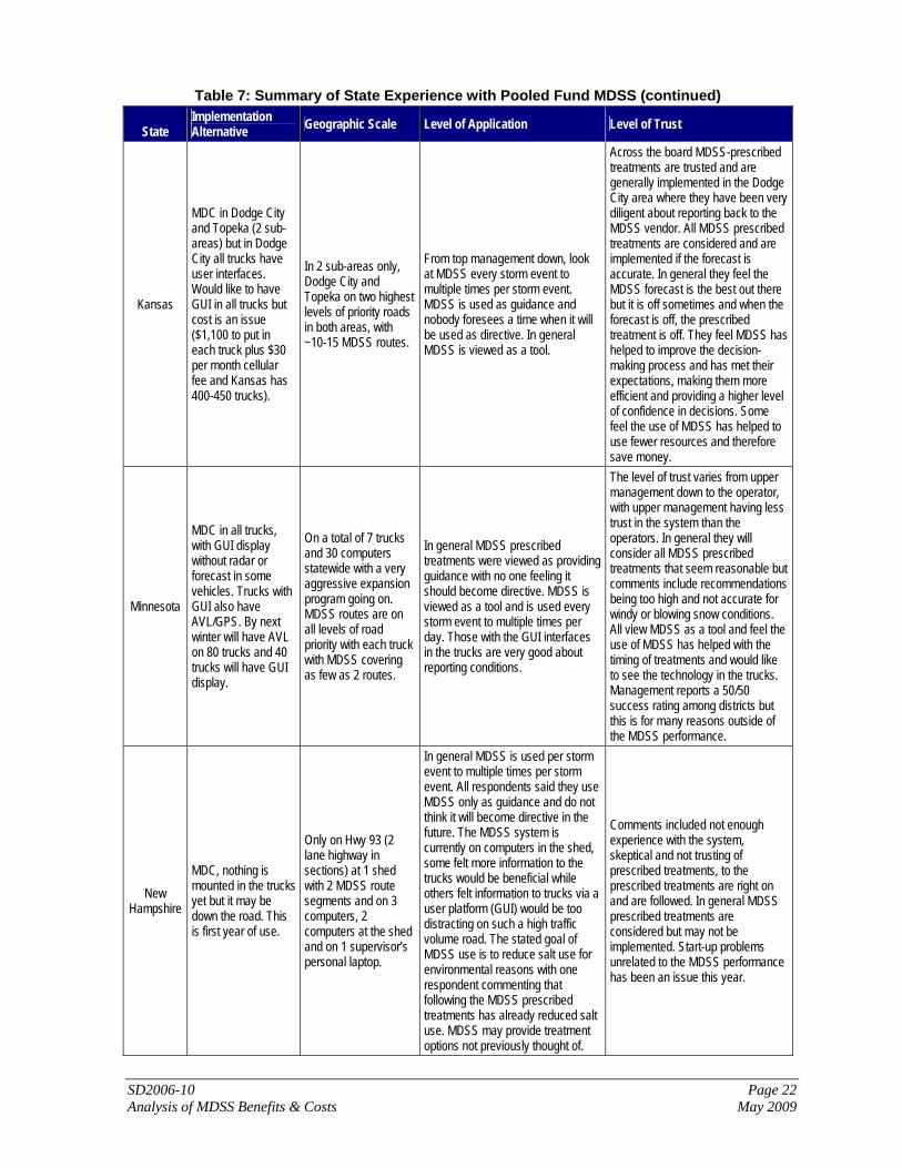
SD2006-10 Page 22 Analysis of MDSS Benefits & Costs May 2009
Table 7: Summary of State Experience with Pooled Fund MDSS (continued)
State Implementation Alternative Geographic Scale Level of Application Level of Trust
Kansas
MDC in Dodge City and Topeka (2 sub-areas) but in Dodge City all trucks have user interfaces. Would like to have GUI in all trucks but cost is an issue ($1,100 to put in each truck plus $30 per month cellular fee and Kansas has 400-450 trucks).
In 2 sub-areas only, Dodge City and Topeka on two highest levels of priority roads in both areas, with ~10-15 MDSS routes.
From top management down, look at MDSS every storm event to multiple times per storm event. MDSS is used as guidance and nobody foresees a time when it will be used as directive. In general MDSS is viewed as a tool.
Across the board MDSS-prescribed treatments are trusted and are generally implemented in the Dodge City area where they have been very diligent about reporting back to the MDSS vendor. All MDSS prescribed treatments are considered and are implemented if the forecast is accurate. In general they feel the MDSS forecast is the best out there but it is off sometimes and when the forecast is off, the prescribed treatment is off. They feel MDSS has helped to improve the decision-making process and has met their expectations, making them more efficient and providing a higher level of confidence in decisions. Some feel the use of MDSS has helped to use fewer resources and therefore save money.
Minnesota
MDC in all trucks, with GUI display without radar or forecast in some vehicles. Trucks with GUI also have AVL/GPS. By next winter will have AVL on 80 trucks and 40 trucks will have GUI display.
On a total of 7 trucks and 30 computers statewide with a very aggressive expansion program going on. MDSS routes are on all levels of road priority with each truck with MDSS covering as few as 2 routes.
In general MDSS prescribed treatments were viewed as providing guidance with no one feeling it should become directive. MDSS is viewed as a tool and is used every storm event to multiple times per day. Those with the GUI interfaces in the trucks are very good about reporting conditions.
The level of trust varies from upper management down to the operator, with upper management having less trust in the system than the operators. In general they will consider all MDSS prescribed treatments that seem reasonable but comments include recommendations being too high and not accurate for windy or blowing snow conditions. All view MDSS as a tool and feel the use of MDSS has helped with the timing of treatments and would like to see the technology in the trucks. Management reports a 50/50 success rating among districts but this is for many reasons outside of the MDSS performance.
New Hampshire
MDC, nothing is mounted in the trucks yet but it may be down the road. This is first year of use.
Only on Hwy 93 (2 lane highway in sections) at 1 shed with 2 MDSS route segments and on 3 computers, 2 computers at the shed and on 1 supervisor’s personal laptop.
In general MDSS is used per storm event to multiple times per storm event. All respondents said they use MDSS only as guidance and do not think it will become directive in the future. The MDSS system is currently on computers in the shed, some felt more information to the trucks would be beneficial while others felt information to trucks via a user platform (GUI) would be too distracting on such a high traffic volume road. The stated goal of MDSS use is to reduce salt use for environmental reasons with one respondent commenting that following the MDSS prescribed treatments has already reduced salt use. MDSS may provide treatment options not previously thought of.
Comments included not enough experience with the system, skeptical and not trusting of prescribed treatments, to the prescribed treatments are right on and are followed. In general MDSS prescribed treatments are considered but may not be implemented. Start-up problems unrelated to the MDSS performance has been an issue this year.

SD2006-10 Page 23 Analysis of MDSS Benefits & Costs May 2009
Table 7: Summary of State Experience with Pooled Fund MDSS (continued)
State Implementation Alternative Geographic Scale Level of Application Level of Trust
North Dakota
MDC with AVL in 8 units.
In Dickerson County all 11 sections have MDSS on 15 computers and in 4 trucks. In Grand Forks County MDSS is on 4 roads on high level priority roads, on a computer in the shed, with no user interfaces in the trucks. In Fargo County MDSS is on 7-10 sections and on computers in all sheds. MDSS is also on 4-5 state headquarters computers and on computers at all 8 district headquarters, ~80 computers statewide.
MDSS is used as a tool. Respondents commented that they use MDSS per storm event to multiple times per storm event. All respondents commented they view MDSS treatment recommendations as guidance, half said they can foresee MDSS treatment recommendations being used as directive while the other half cannot. In general all respondents commented that they will consider MDSS prescribed treatments but may not implement them. All respondents feel MDSS could be best used if information was going to the trucks.
Comments ranged from overall not everyone trusts the MDSS prescribed treatments to yes I trust the treatments but only use them 50% of the time. All respondents feel the MDSS has met their expectations. All respondents commented that they feel the use of MDSS has helped to increase road safety, mobility and reduced costs.
South Dakota
MDC with limited deployment of GUI units that will have live forecast and radar.
2 sheds have MDSS on 5 or 6 actual roads with 10 MDSS routes. All MDSS routes are on level 2 priority roads (major farm to market roads). MDSS is on computers in each shed but have had trouble with the computers being too slow. 4 trucks will have GUI with forecast and radar by end of season.
In general MDSS is used per storm event to multiple times per storm. All view MDSS as guidance, a tool, and not as directive. Most state liability as the main issue but also mentioned cost (estimated ~$20k for 1 truck with GUI with radar and forecast service). All felt that MDSS would be more valuable if the GUI unit with forecast and radar was in every truck.
In general most feel they do not fully trust the MDSS system yet but all said with time the level of trust is increasing. Some respondents commented that they would not even consider a MDSS prescribed treatment if it did not coincide with their gut feeling, while other have tried one truck using 100% MDSS prescribed treatments for comparison. Some feel MDSS has met their expectations while others feel it has not. Some respondents feel the use of MDSS has helped to reduce product use, save money and increase road safety.
Wyoming
MDC in all trucks with IWAPI and AVL in 5 trucks at each site, Evanston and Cheyenne.
MDSS is in 2 sheds and on computers at the two sheds, also on a couple personal home computers. Last winter ran MDSS only on computers in sheds, this year there are the IWAPI units. One site has 5 MDSS routes on 3 segments of interstate.
In general MDSS is used as tool and is looked at on a per storm basis to multiple times per storm event. All respondents commented that they view MDSS as guidance and do not foresee a time when it will be used as directive. Most respondents also commented that it would be most beneficial if there was GUI in the trucks but one respondent felt this may not be true based on the driver’s experience and capability.
In general respondents felt that MDSS has met their expectations and that the MDSS prescribed treatments are right on. One respondent did not trust the MDSS prescribed treatments. All respondents commented that they would consider suggested treatments and half said they would then implement the suggestions. In general respondents feel MDSS has helped to improve road safety and reduce costs. One respondent commented that MDSS has good event timing.

SD2006-10 Page 24 Analysis of MDSS Benefits & Costs May 2009
5. METHODOLOGY The goal of this research project is to conduct a benefit-cost analysis of MDSS that will provide applicable results for all pooled fund member states. It was intended that the research team would follow the traditional benefit-cost analysis methodology to conduct this research. However, this analysis defies traditional benefit-cost analysis rules in two ways.
Benefit-cost analysis typically relies on a clearly defined base case. In the case of pooled fund states, there is no clear consensus of base cases across the states. Different states employ a variety of information and treatment tools, and also have different accounting and management structures.
Benefit-cost analysis is usually employed to compare a set of well-defined alternatives. In the present case, the MDSS implementation alternatives are not obvious, as there are a variety of considerations related to geographic scale of implementation, the use of MDSS-enabling technologies (e.g. mobile data collection and in-vehicle graphic user interfaces), and the level to which MDSS is actually used.
These and other challenges make it difficult to immediately define how this benefit-cost analysis conforms to the standard FHWA guidelines (8). In reality, the methodology for this project is itself the result of some careful considerations of the complexity of this analytical challenge. Therefore, while this chapter will ultimately describe the benefit-cost methodology applied to the MDSS analysis in terms comparable to FHWA practice, it is necessary to first describe how the methodology was developed. The development proceeded by first considering the objectives associated with winter maintenance and then translating those objectives to benefits and costs. With that structure in place, the end of this chapter highlights how the benefit-cost analysis practices recommended by FHWA line up with the proposed analysis method.
5.1 Definitions Prior to consideration of the objectives of winter maintenance operations, it is necessary to define a few terms which will be used throughout the rest of this document, because of different ways that terms are defined across the pooled fund states.
Level of Service (LOS) refers to the actual pavement condition with respect to accumulation of liquid or frozen precipitate. Level of service is used as a means of categorizing the outcome of winter maintenance operations. This term is used differently in some pooled fund states. Some states use level of service to refer to the treatment policies for a specific road, such as “plow up to 16 hours per day as conditions warrant”. Other states may use level of service as a performance measure, but without direct connection to pavement condition (for example, the number of hours until normal pavement condition is restored).
A route segment is a bi-directional portion of a single highway with fixed end points that is maintained by personnel in a single shed. The pooled fund MDSS application uses the term route segment as a way of describing a section of road that receives generally consistent winter maintenance treatment (with some exceptions on grades and shaded areas).
Rules of practice are the methods that a transportation agency uses in treating its roadways. These include recommendations on use of pre-treatment, conditions under which certain chemicals or materials should be applied, and desired application rates. Not all states have documented their rules of practice. In states that have documented their rules of practice, there may be discrepancies between how the state actually conducts winter maintenance operations and what the documentation stipulates. This may be because the documented rules are overly conservative and will not restore the road quickly enough in some conditions, because of limitations in staffing and materials resources, or because of other factors.

SD2006-10 Page 25 Analysis of MDSS Benefits & Costs May 2009
Shed refers to the smallest maintenance management unit within a department of transportation. Sheds may be referred to by other names, such as unit, garage, section, shop, truck station, or yard. Each shed will usually have multiple route segments under its direct responsibility.
5.2 MDSS and Winter Maintenance Objectives In surveys of MDSS pooled fund states, mobility and safety were continually mentioned as primary objectives of winter maintenance operations. While the order of emphasis changed from state to state and other objectives such as environmental stewardship and cost effectiveness were mentioned, mobility and safety were paramount. Winter maintenance operations focus on the pavement LOS and seek to improve the pavement surface during and after winter weather events. Winter maintenance operations work to improve LOS more quickly than would occur in natural processes such as melting and runoff. Several studies have documented that crash rates increase significantly during winter weather conditions, and that vehicle speeds drop during those conditions as well. These two empirically confirmed theories reveal an interesting phenomenon in driver behavior. Drivers typically recognize when pavement surface conditions require greater caution by reducing speed and increasing following distance between successive cars. However, drivers often underestimate the amount of correction that is needed for current conditions, causing safety problems to multiply. With this in mind, it is important to state that the objective of winter maintenance operations is not zero delay or zero crashes, since mobility and safety reflect factors beyond the control of maintenance professionals. Rather, the objective is to improve the LOS, restoring the pavement to normal operations more quickly. The primary way that MDSS meets this objective is by providing information that can allow maintenance personnel to “stay on top of” a winter event an not be overwhelmed by it. It also allows maintenance personnel to see when a forecasted weather event will overwhelm available resources. This information may include improved forecasts and appropriate pre-treatment recommendations that will shorten the duration of time in which the road’s LOS is operating at below normal conditions (i.e. “recovery duration”; see 9). This, in turn, should have positive benefits in reducing delay and improving safety. Under a given operational philosophy, the level of service improves only with an increase in personnel, material, and financial resources. The relationship between level of service and winter maintenance costs is represented in Figure 12. An agency operating under a baseline condition, following its standard rules of practice, might operate at point 1. Additional or fewer resources would move the agency along the curve labeled “Baseline”. If an agency implements MDSS, it is anticipated that this would move the agency to a curve labeled “MDSS”, on which it is assumed that the same level of resource investment would yield a better level of service. It is not clear where on the curve the agency might fall. An agency could continue to devote the same resources to winter maintenance operations, which would put the agency at point 2 on the MDSS curve. In this case, there are no savings in resources due to MDSS, but instead a level of service improvement results. Another agency may elect to maintain the same level of service and choose to economize on winter maintenance costs. This would be represented as point 3. It is most likely that an agency implementing MDSS would fall somewhere between points 2 and 3, seeking to achieve both a level of service improvement and a reduction in winter maintenance costs.

SD2006-10 Page 26 Analysis of MDSS Benefits & Costs May 2009
Figure 12: Relationship between LOS and Costs
To highlight this tradeoff, the research team used three scenarios to examine MDSS. These scenarios represent different tradeoffs between the benefits that may be realized by agency users and by the traveling public.
Scenario 1 (Base Case). Assuming under a baseline condition by following rules of practice, how much would winter maintenance costs be?
Scenario 2 (Same Resources). Assuming that winter maintenance costs are kept constant and MDSS treatment recommendations are followed, what would be the resulting level of service under MDSS use?
Scenario 3 (Same Condition). Assuming that level of service is kept constant and MDSS treatment recommendations are followed, what would be the resulting winter maintenance costs when MDSS is used?
5.3 Assessing MDSS Benefits This section provides a high-level description of how MDSS was used as a simulator for assessing benefits, and delineates the types of benefits that were assessed.
5.3.1 Use of MDSS as Simulation Tool As illustrated in Figure 12, the use of MDSS may affect both winter maintenance costs and the level of service achieved. The Baseline curve represents the relationship between LOS and winter maintenance costs under a scenario where the agency uses its rules of practice. The MDSS curve represents how the relationship between LOS and winter maintenance costs would be expected to change as a result of using MDSS to its maximum capabilities. Conceptually, the benefits of MDSS can be measured by comparing the two curves shown in Figure 12. This is complicated by several issues, primarily transportation agencies’ general lack of actual LOS measurements that could be used to derive the Baseline curve. Even if the Baseline curve were known, one would need to know to what extent an agency was using MDSS’ capabilities, and where on the MDSS curve between points 2 and 3 the agency chose to balance the tradeoff between winter maintenance costs and LOS.
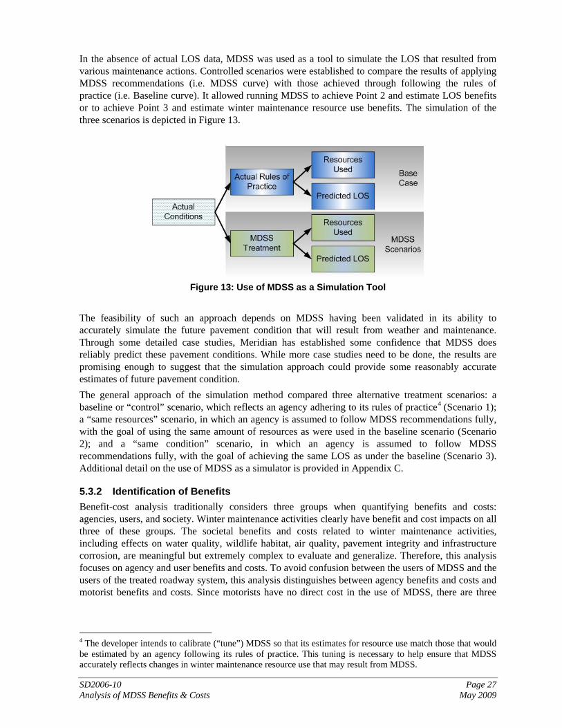
SD2006-10 Page 27 Analysis of MDSS Benefits & Costs May 2009
In the absence of actual LOS data, MDSS was used as a tool to simulate the LOS that resulted from various maintenance actions. Controlled scenarios were established to compare the results of applying MDSS recommendations (i.e. MDSS curve) with those achieved through following the rules of practice (i.e. Baseline curve). It allowed running MDSS to achieve Point 2 and estimate LOS benefits or to achieve Point 3 and estimate winter maintenance resource use benefits. The simulation of the three scenarios is depicted in Figure 13.
Figure 13: Use of MDSS as a Simulation Tool
The feasibility of such an approach depends on MDSS having been validated in its ability to accurately simulate the future pavement condition that will result from weather and maintenance. Through some detailed case studies, Meridian has established some confidence that MDSS does reliably predict these pavement conditions. While more case studies need to be done, the results are promising enough to suggest that the simulation approach could provide some reasonably accurate estimates of future pavement condition. The general approach of the simulation method compared three alternative treatment scenarios: a baseline or “control” scenario, which reflects an agency adhering to its rules of practice4 (Scenario 1); a “same resources” scenario, in which an agency is assumed to follow MDSS recommendations fully, with the goal of using the same amount of resources as were used in the baseline scenario (Scenario 2); and a “same condition” scenario, in which an agency is assumed to follow MDSS recommendations fully, with the goal of achieving the same LOS as under the baseline (Scenario 3). Additional detail on the use of MDSS as a simulator is provided in Appendix C.
5.3.2 Identification of Benefits Benefit-cost analysis traditionally considers three groups when quantifying benefits and costs: agencies, users, and society. Winter maintenance activities clearly have benefit and cost impacts on all three of these groups. The societal benefits and costs related to winter maintenance activities, including effects on water quality, wildlife habitat, air quality, pavement integrity and infrastructure corrosion, are meaningful but extremely complex to evaluate and generalize. Therefore, this analysis focuses on agency and user benefits and costs. To avoid confusion between the users of MDSS and the users of the treated roadway system, this analysis distinguishes between agency benefits and costs and motorist benefits and costs. Since motorists have no direct cost in the use of MDSS, there are three
4 The developer intends to calibrate (“tune”) MDSS so that its estimates for resource use match those that would be estimated by an agency following its rules of practice. This tuning is necessary to help ensure that MDSS accurately reflects changes in winter maintenance resource use that may result from MDSS.

SD2006-10 Page 28 Analysis of MDSS Benefits & Costs May 2009
components that are then included in this evaluation methodology: agency benefits, motorist benefits, and agency costs5. Agency costs will be further addressed in Section 5.4.
5.3.2.1 Agency Benefits The primary agency benefit of MDSS is reduction in winter maintenance resources which are used. While the agency benefits from improvements in LOS, the real beneficiary of LOS improvements is the traveling public. Therefore, to avoid double-counting, agency benefits are limited to the question of resource use. The agency benefit from using MDSS was reflected as the difference in costs (labor, materials and equipment) resulting from using MDSS. By using the simulation-based methodology in this study, only material costs were included for the quantification of agency benefits.
5.3.2.2 Motorist Benefits Motorists receive a variety of benefits through winter maintenance operations. A landmark FHWA study in 1977 assessed economic impacts of winter maintenance in traffic and safety in three categories: time delay, accidents, and other costs (10). Each of these categories considered a wide range of impact areas. Time delay included comfort and convenience, operating costs to cars and trucks, and wage loss due to tardiness. Other costs included product spoilage and product losses. The same study, as well as more recent studies by Thornes (11, 12), include fuel savings. For the purposes of this study, the research team focused on two motorist benefits: mobility and safety 6. These correspond with the primary outcome objective of winter maintenance operations, which is to improve the roadway level of service. An extensive literature review was conducted to identify studies that correlated roadway level of service to traveler speed or safety. The team identified approximately 30 different studies that examined the effects of winter weather on speeds and safety as summarized in Appendix D. Mobility. Mobility-related motorist benefits focus on reductions in delay that may result from MDSS use. Delay is reduced as motorist speed is able to increase safely as a result of improvements in the level of service. The difference in estimated delay can be multiplied by an estimate of the value of time to calculate the economic benefit of reduced delay. Reduced delay is calculated by comparing the total travel time under the baseline scenario with that under the MDSS scenario. Improvements in level of service would result in improvements in travel speed and reductions in delay. Calculations of delay savings require knowledge about: the amount of time that a route segment is at a given level of service; the traffic volume, free-flow speed 7 and length associated with that route segment; and the travel speed effects associated with a certain degradation in level of service. The research team is not aware of any studies that specifically correlate level of service with driver speed. Many studies, however, have correlated weather conditions with driver speed (e.g. 13, 14, 15, 16). These studies have generally focused on rural highways and have calculated speed reduction in terms of the numerical reduction in miles per hour. For simplicity, the research team assumes that the speed
5 Traditional benefit-cost analysis regards these components as having equal weight; in other words, a dollar of agency benefits is analytically equivalent to a dollar of motorist benefits. In practice, an agency may adopt a different approach, where agency benefits are treated as having greater importance than motorist benefits, since the level of motorist benefits may not be as easy to perceive. 6 Both of Thornes’ studies indicate that fuel savings comprises less than 1 percent of the motorist benefits of winter maintenance. 7 Posted speed limit will be used as a proxy for free-flow speed; see Appendix F for elaboration.

SD2006-10 Page 29 Analysis of MDSS Benefits & Costs May 2009
reduction associated with a specific level of maintenance is based on a percentage of the speed limit of the roadway. This is presented in mathematical form in Appendix E. Safety. The approach for calculating safety benefits associated with a change in level of service is similar to that used for delay. A crash rate can be established from historic safety data for a given road segment over a specific time period. This crash rate can be associated with applying the rules of practice over the same time period. Building on previous studies which have sought to quantify the effects of weather conditions on highway safety (e.g. 14, 15, 17), a basic crash rate was calculated. This basic crash rate is the crash rate that would occur if no adverse weather was experienced on that route segment, and is assumed to be a property of the route segment. Then, the results of the MDSS simulation can be used to extrapolate the expected crash rate that would result from improvements in level of service. This is described in more detail in Appendix F.
5.3.3 Risks Affecting Estimation of Benefits Two major risk factors affect the estimation of benefits: less than full use of MDSS and the relative severity of winters.
5.3.3.1 Implementation Levels of MDSS As discussed earlier, the simulation approach compares a Baseline scenario to an MDSS scenario that assumes 100 percent adherence to MDSS-recommended treatments (i.e. Application 2). No pooled fund state currently uses MDSS at that level, and it may be years before any state does. Section 3.4 identified four factors that help to characterize the implementation of MDSS:
the quality of underlying forecasting services, the reliability of feedback regarding actual treatment activities, the use of treatment recommendations by vehicle operators, and the use of an in-vehicle GUI.
The effect of each of these options on MDSS use can be readily understood. Poor quality forecasts will result in MDSS having poor predictive power, which will undermine user confidence. Poor feedback regarding actual treatment activities will propagate predictive errors. The failure of supervisors or operators to trust MDSS recommendations will limit quantifiable benefit in terms of improved level of service or resource use. An in-vehicle GUI can be effective in communicating what MDSS recommends to the drivers who will implement those recommendations; conversely, the failure of drivers to receive recommendations will prevent their implementation. While the effects of all four of these options can be readily understood, only one can be easily quantified: the extent to which treatment recommendations, once they are received, are actually used. (See Appendix G for a full discussion on why the other factors cannot easily be included in the analysis.) This factor will be included by setting different alternatives regarding the percentage of the time that MDSS treatment recommendations are actually used by vehicle operators. Two alternatives for scenarios 2 and 3 (Figure 12) will be used: 100 percent adherence to treatment recommendations and a percentage value (less than 100 percent) adherence corresponding to a specific state’s situation. Thus, the latter percentage value may vary for each state. The normal MDSS implementation alternative assumes that treatment recommendations are followed 100 percent of the time. The risk is that use levels will be less, meaning that less benefit will be realized.
5.3.3.2 Winter Severity The goal in looking at winter severity is to make sure that any benefits associated with MDSS are rooted in a proper historical context so that they may be more accurately interpreted. MDSS has been implemented on a comparatively recent basis, when weather patterns for a given state may not be in accordance with historic trends. If the winters in which MDSS has been implemented can be

SD2006-10 Page 30 Analysis of MDSS Benefits & Costs May 2009
effectively correlated with long-term climate patterns in a given state, this would help to ensure that the estimated benefits of MDSS may be reasonably expected in the future. The research team’s general approach was to look at winter severity from the perspective of individual storm events. Through mining of historical weather data, the frequencies of various types of storms were identified. A more technical discussion of the team’s approach may be found in Appendix H.
5.4 Assessing MDSS Costs The previous section discussed how the research team classified various benefits that may be associated with MDSS use, including both agency and motorist benefits. It is next necessary to determine the costs of MDSS that would be associated with each use scenario. Costs may be divided into three categories: MDSS vendor costs, weather forecast provider costs, and agency support costs.
5.4.1 MDSS Vendor Costs One particular challenge in estimating the cost of MDSS is that the pooled fund MDSS has been developed as a research project, not explicitly as a profit-maximizing business enterprise. Pooled fund states have been using MDSS on a trial basis as a research project. The vendor has provided support consistent with the resources available to it through project funding. As the research project morphs into an operational product, the cost of MDSS will depend significantly on the level of product support provided by the MDSS vendor. The pooled fund MDSS developer has delineated five considerations that influence the cost of an operational MDSS to a department of transportation (18).
Configuration. Each time MDSS is added on a new route, the route must be configured into the software. Currently, the MDSS vendor has provided that as a part of its research contract support. The cost of providing this in the future will vary significantly based on the quality of data that a transportation department has. For example, does information on snow plow routes, construction, and traffic exist in GIS format? Do maintenance practices vary from route-to-route or garage-to-garage? The vendor estimated that configuration efforts could vary from two weeks to several months for an entire state.
Training. The pooled fund MDSS developer’s experience has been that training is essential to maximizing the value realized from MDSS. Moreover, the full value of training is not realized in a one-time event for a given state. Training is an annual requirement to educate new personnel and to provide a refresher to experienced personnel. Follow-up training sessions appear to increase how well users can take advantage of MDSS’ range of capabilities. Currently, the pooled fund developer has provided MDSS training as a part of its contract, at least once per season per state, with at least one state having dozens of training classes in one season. Several factors influence the cost of training. First, who conducts the training: the MDSS vendor, a third-party under contract, or the transportation department? How many training sessions are performed? Are the training sessions concentrated into a short time frame to economize on travel costs, or are they done at different times before and during a winter season? What training materials are provided? Would a training version of the GUI need to be prepared?
Bandwidth. The pooled fund MDSS vendor currently has two T-1 lines dedicated to supporting existing MDSS use (cost: $1,500 per month). The vendor has indicated that current use levels (number of routes and users) of MDSS are equivalent to what one average-sized state might use in a statewide deployment. Even so, however, there is considerable flexibility in how much bandwidth a state might use, which could lower these costs. For example, can some datasets be dropped because they aren’t used much? What is the update frequency? How many
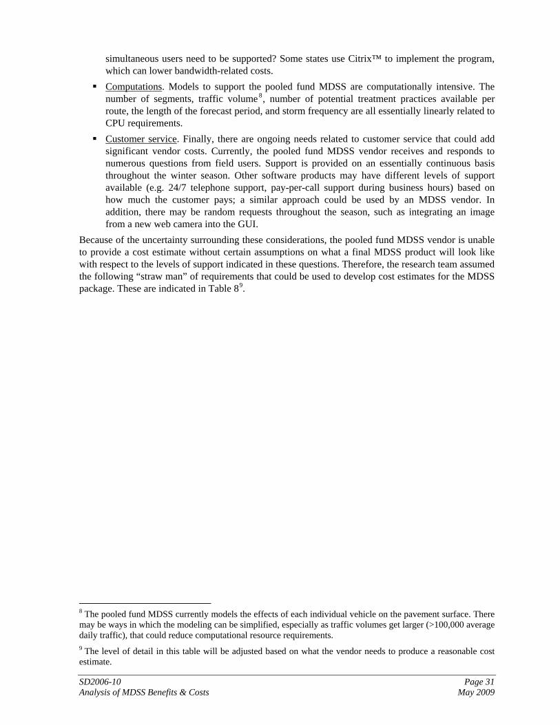
SD2006-10 Page 31 Analysis of MDSS Benefits & Costs May 2009
simultaneous users need to be supported? Some states use Citrix™ to implement the program, which can lower bandwidth-related costs.
Computations. Models to support the pooled fund MDSS are computationally intensive. The number of segments, traffic volume 8, number of potential treatment practices available per route, the length of the forecast period, and storm frequency are all essentially linearly related to CPU requirements.
Customer service. Finally, there are ongoing needs related to customer service that could add significant vendor costs. Currently, the pooled fund MDSS vendor receives and responds to numerous questions from field users. Support is provided on an essentially continuous basis throughout the winter season. Other software products may have different levels of support available (e.g. 24/7 telephone support, pay-per-call support during business hours) based on how much the customer pays; a similar approach could be used by an MDSS vendor. In addition, there may be random requests throughout the season, such as integrating an image from a new web camera into the GUI.
Because of the uncertainty surrounding these considerations, the pooled fund MDSS vendor is unable to provide a cost estimate without certain assumptions on what a final MDSS product will look like with respect to the levels of support indicated in these questions. Therefore, the research team assumed the following “straw man” of requirements that could be used to develop cost estimates for the MDSS package. These are indicated in Table 89.
8 The pooled fund MDSS currently models the effects of each individual vehicle on the pavement surface. There may be ways in which the modeling can be simplified, especially as traffic volumes get larger (>100,000 average daily traffic), that could reduce computational resource requirements. 9 The level of detail in this table will be adjusted based on what the vendor needs to produce a reasonable cost estimate.
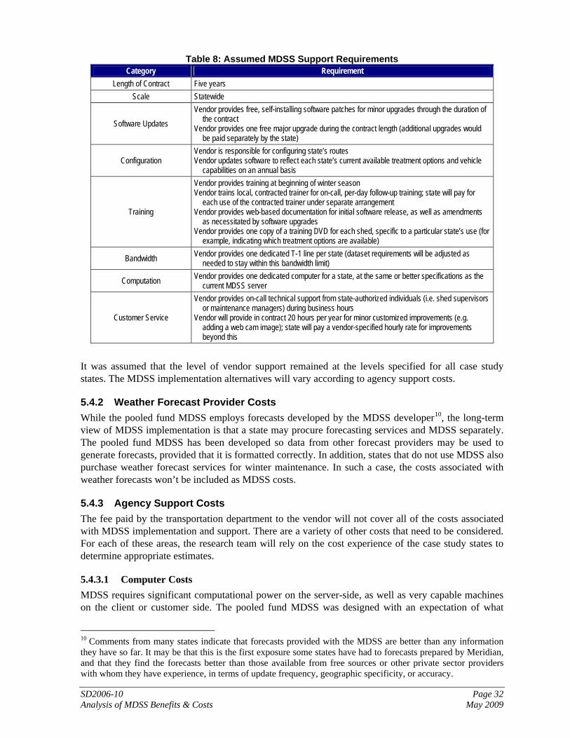
SD2006-10 Page 32 Analysis of MDSS Benefits & Costs May 2009
Table 8: Assumed MDSS Support Requirements Category Requirement
Length of Contract Five years Scale Statewide
Software Updates Vendor provides free, self-installing software patches for minor upgrades through the duration of
the contract Vendor provides one free major upgrade during the contract length (additional upgrades would
be paid separately by the state)
Configuration Vendor is responsible for configuring state’s routes Vendor updates software to reflect each state’s current available treatment options and vehicle
capabilities on an annual basis
Training
Vendor provides training at beginning of winter season Vendor trains local, contracted trainer for on-call, per-day follow-up training; state will pay for
each use of the contracted trainer under separate arrangement Vendor provides web-based documentation for initial software release, as well as amendments
as necessitated by software upgrades Vendor provides one copy of a training DVD for each shed, specific to a particular state’s use (for
example, indicating which treatment options are available)
Bandwidth Vendor provides one dedicated T-1 line per state (dataset requirements will be adjusted as needed to stay within this bandwidth limit)
Computation Vendor provides one dedicated computer for a state, at the same or better specifications as the current MDSS server
Customer Service
Vendor provides on-call technical support from state-authorized individuals (i.e. shed supervisors or maintenance managers) during business hours
Vendor will provide in contract 20 hours per year for minor customized improvements (e.g. adding a web cam image); state will pay a vendor-specified hourly rate for improvements beyond this
It was assumed that the level of vendor support remained at the levels specified for all case study states. The MDSS implementation alternatives will vary according to agency support costs.
5.4.2 Weather Forecast Provider Costs While the pooled fund MDSS employs forecasts developed by the MDSS developer10, the long-term view of MDSS implementation is that a state may procure forecasting services and MDSS separately. The pooled fund MDSS has been developed so data from other forecast providers may be used to generate forecasts, provided that it is formatted correctly. In addition, states that do not use MDSS also purchase weather forecast services for winter maintenance. In such a case, the costs associated with weather forecasts won’t be included as MDSS costs.
5.4.3 Agency Support Costs The fee paid by the transportation department to the vendor will not cover all of the costs associated with MDSS implementation and support. There are a variety of other costs that need to be considered. For each of these areas, the research team will rely on the cost experience of the case study states to determine appropriate estimates.
5.4.3.1 Computer Costs MDSS requires significant computational power on the server-side, as well as very capable machines on the client or customer side. The pooled fund MDSS was designed with an expectation of what
10 Comments from many states indicate that forecasts provided with the MDSS are better than any information they have so far. It may be that this is the first exposure some states have had to forecasts prepared by Meridian, and that they find the forecasts better than those available from free sources or other private sector providers with whom they have experience, in terms of update frequency, geographic specificity, or accuracy.
SD2006-10 Page 33 Analysis of MDSS Benefits & Costs May 2009
computational resources would likely be normative at the users’ sites. Over time, the MDSS developer reports that user complaints about MDSS being slow have been less frequent, as users’ computers have been upgraded through normal replacement processes. It may be expected that a user will have a workstation at each shed which may or may not be dedicated to MDSS. Use of MDSS could require improvements in client-side bandwidth.
5.4.3.2 Training As MDSS becomes operational, it is uncertain how training on MDSS might be integrated with other winter maintenance training. Currently, MDSS training occurs as a separate, added class for maintenance personnel, although the class provides information that could supplement and reinforce material provided through other training (whether or not provided by the DOT). Even under a vendor-provided scenario, therefore, the training has a cost in terms of the value of time of maintenance personnel. Additional training costs may also be borne by the DOT. One option that many states may pursue is to have a “train-the-trainer” approach, where the MDSS vendor trains a champion within each state (or perhaps one at each region), and then that DOT employee travels elsewhere in the state to train the state’s employees. There would be costs associated with the value of the trainer’s time, as well as travel. If the state chooses to rely on vendor or third-party training options, these will have their associated costs as well. The costs of training have currently been borne solely by the pooled fund MDSS vendor. Follow-up with the case study states will be necessary to determine what type of training they would most likely pursue, given the more limited training requirements imposed upon the vendor in Table 8.
5.4.3.3 Administrative Costs There may be other costs that an agency pays to implement MDSS, such as project management, contract management, and coordination of user registrations.
5.4.3.4 Technology Options As was noted earlier, a state may use mobile data collection or in-vehicle GUI to improve the utility of MDSS. MDC involves three major types of costs. First, is the purchase cost associated with in-vehicle data collection, including an on-board touchscreen interface (or similar device), along with any improvements in on-board sensors, such as plow position switches or improved spreader controllers, that are necessary to provide MDSS the appropriate level of data. Second, MDC requires a communication system to transmit information on recent maintenance activities back toward the MDSS server. This communication requirement will usually be handled through an existing trunk radio system or cellular communications. Third, MDC will require on-going support from the MDC equipment vendor(s). This may be included in the purchase cost or it could be an extended warranty arrangement. The costs of the in-vehicle GUI will involve similar components as for MDC. States may opt to use the in-vehicle GUI with or without MDC.
5.5 Benefit-Cost Analysis The crux of the benefit-cost analysis is a comparison of the total benefits and total costs associated with a project. The benefits and costs calculated in the previous sections were compared using a ratio to determine the relative cost-effectiveness of various MDSS implementation alternatives. (More information on these alternatives is provided in Appendix G.) In preparing this benefit-cost analysis approach, the research team referenced guidelines published by the FHWA regarding how to conduct a benefit-cost analysis (9). Understanding that these guidelines
SD2006-10 Page 34 Analysis of MDSS Benefits & Costs May 2009
were developed in the context of evaluating alternative highway improvement projects, not all are applicable to this present analysis11. This section summarizes how the described procedure correlates with the FHWA recommended practice.
5.5.1 Scope (Step 0) One step not included in the FHWA guidelines, but of particular relevance to the MDSS analysis, is the establishment of the scope of the analysis. To economize on resources, the research team used a case study approach, where three states were selected from among the pooled fund states for analysis. These states were selected from among three climatologically similar groupings:
Mountain/West States: California, Colorado, and Wyoming Northern Plains States: Iowa, Minnesota, North Dakota, and South Dakota Transition (Freezing Rain) States: Indiana, Kansas, New Hampshire, New York, and Virginia
Several factors need to be present for a state to be an effective case study. The state must have good historical data on winter maintenance resource use to permit “tuning”
of MDSS. This would ideally be data recorded with daily observations for specific road segments over the course of five or six winters.
The state must have documented rules of practice, or records of maintenance activities at a truck-run level (i.e. a separate record of each truck’s activities, including time of run start, beginning and ending mileposts, and chemical/material application rates, for each route it covers). These are again required to tune MDSS to validate the resource use estimates that may result from simulation.
The state must have data on its system that supports estimation of motorist benefits. These include posted speed limits, annual average daily traffic (AADT) volumes, monthly traffic volumes for selected routes (to AADT volumes to match typical winter volumes), the lengths of highway segments, and counts of the number of crashes arising over the same winters over which the MDSS simulation is run.
The state must also have data that would support estimation of the costs of MDSS implementation. In general, states with the most experience with MDSS will be best able to quantify the types and magnitudes of costs associated with statewide implementation.
The case studies were selected by working with pooled fund member states to see which states best match all of these criteria. Together, these states were intended to provide a good cross-section such that the results would be reasonably transferable to other pooled fund states. Based on outreach to the pooled fund states conducted by the research team, Colorado, Minnesota, and New Hampshire were used as case study states. A state may conceivably adopt MDSS on a piecemeal basis, focusing on certain regions or corridors. This makes sense especially in terms of the cost of acquiring in-vehicle equipment to support MDC or in-vehicle GUI. For the purposes of this analysis, it was assumed that MDSS will be adopted on a statewide basis. The results of the benefit-cost analysis, if sufficiently favorable from a state’s investment perspective, can be used to portray the long-term gains that can be realized through scaled implementation of MDSS. Therefore, it should still provide value to states that may not have the resources for implementing statewide coverage all at once. One state from each climatologic group was finally chosen based on the above criteria. These states are New Hampshire (a transition state), Minnesota (a northern plains state), and Colorado (a
11 Steps 5 (define level of effort for screening alternatives) and 6 (analyze traffic effects) were omitted since they do not apply to this assessment.

SD2006-10 Page 35 Analysis of MDSS Benefits & Costs May 2009
mountain/west state). This research project used these state case studies to evaluate the benefits and costs associated with the use of MDSS.
5.5.2 Establish Objectives (Step 1) As noted earlier, the primary objective of winter maintenance operations is to keep the level of service at a good level within resource constraints in order to maximize safety and mobility for motorists. Since level of service improvements will enhance both safety and mobility, there is no need to use different objectives for different states. The political context of some agencies may mean that, in practice, different values to a dollar spent by agency personnel and a dollar saved by the motoring public. This is especially true in cases where the benefits received by the public may be marginally perceptible (e.g. 30 seconds in savings per vehicle on a given route segment). Under a benefit-cost analysis framework, however, all benefits and costs are treated equally, whether they are borne by the agency or motorists. The use of a variety of scenarios as described earlier (keeping resources fixed and improving LOS, keeping LOS fixed and saving resources, and a combination) can help an agency to see the tradeoffs that may be involved between agency and motorist benefits with MDSS. The agency can then judge within its own political context whether an MDSS investment makes sense.
5.5.3 Identify Constraints and Specify Assumptions (Step 2) The research team’s approach to this analysis respects the existing constraints within each case study state’s winter maintenance operations. These constraints reflect rules of practice, resource availability, and treatment methods in use. It is possible that MDSS may affect some of these constraints over the long term but, to be conservative, the research team assumed those constraints would still be in place. There are two types of assumptions that may be considered: methodological assumptions and parameter value assumptions. Methodological assumptions are used as necessary stepping stones in completing the logical connection between data and results. Parameter value assumptions are quantitative inputs which are estimated based on professional judgment and can be changed to test the sensitivity of model results to these parameters. The following lists methodological assumptions that were presented through earlier sections in this document:
1. Societal benefits, such as reduced degradation of water quality and wildlife habitat, are not considered in this analysis.
2. Motorist benefits are assumed to be limited to safety improvements and delay reduction. 3. MDSS use may result in reductions in winter maintenance costs (better use of resources),
improved level of service (better outcomes), or both. 4. Daily traffic volumes during the winter months may be estimated from annual average daily
traffic volumes by multiplying by an appropriate seasonal adjustment factor. 5. Vehicle Miles Traveled (VMT) will not be decreased to reflect storm-related trip reduction. 6. Weather severity can be reasonably modeled using a storm-based approach. 7. National Weather Service (NWS) data, obtained through the National Climatic Data Center,
should approximate weather data in the road environment well enough for climatological purposes.
8. Storm types may be identified by certain signatures of various weather parameters. 9. The weather conditions at one site should provide approximate representation of climatological
fluctuations within an entire shed.

SD2006-10 Page 36 Analysis of MDSS Benefits & Costs May 2009
10. For purposes of delay estimation, travel time will be based on posted speed limits. (See Appendix E for a more detailed justification of this assumption.)
11. MDSS provides reasonably accurate estimates of future pavement condition when a specific maintenance treatment is applied to certain road weather conditions.
The following are parameter value assumptions. 1. The relative average costs of materials may be used as a guide for estimation of future winter
maintenance cost savings. 2. The average value of travel time is 75 percent of the local wage rate (19, 20). This is conservative
in that it doesn’t capture the higher value of time for freight movements or the complications of “synchronous activities” (14), such as just-in-time logistics.
3. Motorist speed degrades at certain rates based on pavement level of service. 4. Crash rates tend to increase as level of service deteriorates, using fixed factors based on a
baseline crash rate for each roadway.
5.5.4 Define Base Case and Identify Alternatives
5.5.4.1 Base Case Development of the base case is critical to benefit-cost analysis, as the selection of an unrealistic base case is considered by the FHWA to be the greatest source of error in benefit-cost analysis (9). Interviews with states confirmed that defining the base case for each state is quite challenging, however. Each state represents a different combination of winter maintenance philosophies, information sources used, treatment options available, and other factors. To overcome this difficulty, the methodology defines the base case as a “non-MDSS” case using a state’s standard rules of practice. Using data from several recent winter seasons, the methodology reflects data that includes the entirety of use circumstances in each case study state, and the way the state normally handles winter maintenance operations.
5.5.4.2 Implementation Alternatives As described earlier, the analysis compares the Base Case with MDSS scenarios (Same Condition and Same Resources), which presume full use of MDSS, including following all treatment recommendations. These two scenarios assume universal deployment of MDC capabilities.
5.5.5 Set Analysis Period (Step 4) The analysis period is important because of the different time scales associated with different winter maintenance costs. To ensure that alternatives can be compared fairly, one benefit-cost analysis primer recommends, “The costs and benefits of an option are to be evaluated over a timeframe equivalent to the economic (useful) life of the associated facilities/assets affected by the decision.” (21) The simulation approach will focus on estimates of resource use without any ties to dollars. Therefore, it will be easy to convert the resource estimates to current year costs. The research team used a five-year investment cycle. There are several factors that will likely cause significant change to winter maintenance operations over the next few years. For example, there may be improved availability of communications infrastructure, which could reduce agency costs. Adoption of anti-icing practices, which necessitates detailed information about storm timing, is expected to increase. New chemicals may offer cost savings and improved performance, extending the capabilities of what tailored treatment recommendations could do. Impending retirements among experienced maintenance personnel may increase the need for accelerated training, which MDSS could support. Within MDSS, there will be

SD2006-10 Page 37 Analysis of MDSS Benefits & Costs May 2009
continued efforts by many states to push and extend its capabilities, to include fleet management and resource management functions, and potentially to assist with planning timescale decisions (e.g. where to locate material storage facilities). Some burgeoning efforts to expand decision support tools for other aspects of weather and maintenance could gain traction, providing additional benefits with minimal additional cost. While these factors seem to support or encourage implementation of MDSS, it would be difficult to quantify them in the analysis. Therefore, it would be conservative to ignore these factors in the analysis, with the idea that future benefits may be better than indicated by the model results.
5.5.6 Estimate Benefits and Costs Relative to Base Case (Step 7) Three types of benefits and costs are associated with transportation projects: agency, user (labeled as “motorists” in this document to avoid confusion with agency users of MDSS), and society. A taxonomy of these benefits and costs are provided in Table 9. For consistency sake, reductions in agency costs are treated as agency benefits.
Table 9: Taxonomy of MDSS Benefits and Costs Agency Motorist Society Benefit Reduced materials costs
Reduced labor costs Reduced equipment costs Reduced fleet replacement costs Reduced infrastructure damage due
to road salts
Reduced motorist delay (through improved LOS)
Improved safety (through improved LOS)
Reduced response time Reduced clearance time Reduced vehicular corrosion due to
road salts
Reduced environmental degradation
Cost Software and support costs Communications costs In-vehicle computer hardware
investment Training Administrative costs Weather forecast provider costs
Bold indicates included in methodology
5.5.7 Evaluate Risk (Step 8) A risk assessment seeks to answer three questions (9):
What can happen? How likely is it to happen? and What are the consequences of an event occurring?
There are several risk factors (e.g., user acceptance, winter weather severity) that may affect the results of this analysis. The likelihood of each of the risk factors is not considered in this section. Instead, this section focuses on how the research team accounted for each of these risks in its analysis.
5.5.7.1 Risk 1: User Acceptance The methodology assumes full use of MDSS including treatment recommendations (i.e. Application 2). Non-use of MDSS would be expected to reduce potential agency and motorist benefits. As a result, benefits could be overstated if users are not accepting of the technology.
5.5.7.2 Risk 2: Winter Severity The MDSS simulations will be conducted over a limited number of winter seasons of data. It is possible that the weather data used as input into the simulation is not representative of long-term climatic norms. Benefits could be over- or under-estimated based on the actual winter over which

SD2006-10 Page 38 Analysis of MDSS Benefits & Costs May 2009
observations were collected. For simplicity, this research study assumes that the several winter seasons of data for simulation represent long-term climatic norms.
5.5.8 Compare Net Benefits and Rank Alternatives The research team presented the results of this analysis, and compared the benefit-cost ratios of MDSS scenarios.
5.5.9 Make Recommendations As permitted by the data, the research team offered conclusions as to the conditions in which MDSS benefits appear to outweigh costs. The research team also offered a range of recommendations relating to future MDSS implementation or pre-MDSS activities that could improve the likelihood of successful MDSS implementation.
5.6 Summary The methodology for benefit-cost analysis consists of two modules: the baseline data module and the simulation modules, as shown in figures 5-2 and 5-3, respectively. Figure 14 shows how the winter maintenance cost model was developed and calibrated based on data obtained from each case study state. Figure 15 shows how the calibrated cost model will be applied to develop benefit-cost ratios for each MDSS alternative. Figure 14 and Figure 15 show how MDSS was used as a simulation tool to support the benefit-cost analysis. In the process of benefit analysis, these two modules progress in a parallel sequence instead of a serial sequence. In the baseline data module, various data, including highway route information (step 1), winter maintenance resource use data (step 2), traffic volume (step 3), crash data (step 4), and weather information (step 5), are incorporated to establish detailed baseline information for each route segment. In step 3, truck and non-truck data are tracked separately because trucks have a higher value of travel time. In the simulation module, steps 6 to 8 are used to generate simulation output from MDSS for the each of the three scenarios, based on the inputs of selected route segment(s) for simulation, weather data, daily resource use data, and rules of practice. The process of simulation includes model establishment for a route segment, calibration, and validation. Output from simulation mainly includes pavement conditions (LOS information) and maintenance information by hour.

SD2006-10 Page 39 Analysis of MDSS Benefits & Costs May 2009
Figure 14: Baseline Data Module
Figure 15: Simulation Module

SD2006-10 Page 40 Analysis of MDSS Benefits & Costs May 2009
The process of simulation takes considerable effort even for a route segment. Thus, for a given state, it is recommended that only a few representative sites are used for simulation instead of several hundred highway segments. The representative sites must have good records regarding historical maintenance activities, documented rules of practice, and a nearby weather station. The simulation outputs from selected route segment(s) are then extrapolated to other route segments within the state. The classification of storm events in steps 5 and 9 connects the baseline data module with the simulation module. In step 5, weather data are obtained from weather stations that have sufficient historic data. Winter storm events (that have at least 1 hour of moisture, either as precipitation or condensation, on the roadway) are identified according to a series of weather parameters. As shown in Appendix H, the parameters include air temperature, storm duration, precipitation accumulation, precipitation rate, average wind speed in storm, average wind speed after storm, and condensation. Each parameter includes a range of values and each storm event consists of eight values, each representing a value of the associated parameter. Obviously, there are a large number of potential events with different parameter values under this concept. Thus, storms events need to be further classified into a certain number of groups. Cluster analysis method was used for this purpose. While there are many existing techniques for cluster analysis, the k-means method (22) is used in this study as it is more suitable for cluster analysis when the sample size is large (e.g., >200). K-means is a simple procedure to classify a given dataset through a certain number of clusters (assume k clusters). The algorithm of k-means aims at minimizing the objective function:
∑∑= =
−=k
j
n
ij
ji cxJ
1 1
2
where
2
jj
i cx − is a distance measure between a data point jix and the cluster center jc ,
and J is an indicator of the squared Euclidean distance of the n data points from their respective cluster centers. After events are clustered, the number of storm events per winter season for each cluster (storm type) can be calculated for each route segment, and step 5 is finished. In step 9 of the simulation module, the storm events are also identified according to weather parameter values in Appendix H, based on the weather data collected for simulation. Each storm event is then matched to one of the k clusters determined in step 5. The minimum squared Euclidean distance in Equation 5-1 is used for matching storm events to clusters. The matching means that the baseline data module and the simulation module are connected and the simulation results can be applied to the baseline data module. In step 9c, resource use and road conditions are characterized for each storm type. With this, the average resource use (e.g., amount of material used per storm type per lane mile) and the average duration under various road conditions (e.g., number of hours under “slushy” pavement condition per storm type) can be calculated for each storm type, and for each scenario. The average values are further applied to the baseline data module for benefit analysis. An assumption of the application is that storms of the same type will require a similar winter maintenance response (e.g., resource use). The benefit analysis of resource use is relatively simple. The resources used for each scenario can be easily obtained, given the number of events per storm type per season (derived from step 5e) and the values of resource use (derived from step 9c). The benefit analysis for resource can then be conducted through comparing the total resources used in different scenarios.
SD2006-10 Page 41 Analysis of MDSS Benefits & Costs May 2009
6. ANALYSIS OF TANGIBLE BENEFITS AND COSTS In this chapter, benefit-cost analysis is conducted for three pooled fund states, that belong to different climatologically groups: a transition (freezing rain) state (New Hampshire), a mountain west state (Colorado), and a northern plains state (Minnesota). The analysis is carried out case by case to identify the tangible benefits and tangible costs associated with the use of MDSS. The classification of storm events is first described because it is analyzed based on weather data collected from the three states.
6.1 Storm Identification and Classification Weather data were collected from the NOAA (National Oceanic and Atmospheric Administration)’s NCDC (National Climatic Data Center) web site for these states. Data files contain hourly data and include information of station data, date, time, temperature, wind, visibility, dew point, precipitation, and snow. Weather data were collected from 107 stations with 13 stations in New Hampshire, 61 stations in Minnesota, and 33 stations in Colorado. In total, 2,167 years of weather data were obtained from these stations. Data reduction was conducted prior to the identification and classification of storm events. In this study, two simple rules were applied to data reduction:
Since winter maintenance was carried out during winter season (November 1 of one year to March 31 of the following year), weather data during the five winter season months were retained and those between April 1 and October 31 were discarded.
For each winter season of data, if more than 25 percent of hourly data were missing this season of data was discarded.
After data reduction, 1,435 winter seasons of data from 102 weather stations were qualified for further analysis and 732 winter seasons of data were deleted. The name, location, and elevation of the weather stations, as well as their availability of weather data, are presented in Appendix I. According to the variables (e.g., air temperature range, pavement temperature trend, and storm duration) provided in Appendix H, storm events were identified based on the 1,435 winter seasons of weather data and resulted in a total of 35,795 storm events. The number was further reduced to 34,742, with 1,253 events discarded as one or more variable values were not available due to missing data. The number of storm events after reduction was large enough for reliable storm classification. This large number of storm events made the storm classification results transferable to other pooled fund states. The k-means clustering analysis method was used to classify the identified storm events. A k value of 20 was used, which means that 20 cluster centers will be generated for the identified storm events. After the analysis, the parameter values for each cluster center were obtained, as shown in Table 10. Each cluster center represents a specific location at an eight-dimensional space, which is constrained to the minimum and maximum values of these parameters.

SD2006-10 Page 42 Analysis of MDSS Benefits & Costs May 2009
Table 10: Cluster Centers Variables
Cluster No.
Air Temp. Range
Pavement Temp. Trend
Storm Duration
Precip. Accumu-
lation Precip.
Rate Avg. Wind
Spd.
Avg. Wind Spd. Aft.
Storm Conden-
sation 1 3.77 1.29 5.30 3.59 1.16 1.46 1.57 0.44 2 3.61 1.74 5.10 1.81 1.00 1.27 1.41 0.45 3 1.47 2.02 1.36 2.93 2.80 0.83 1.21 0.23 4 1.70 1.87 3.41 3.49 1.90 1.34 1.37 0.28 5 3.64 2.72 3.45 2.24 1.06 1.48 1.55 0.27 6 3.73 1.73 3.48 3.74 2.39 1.36 1.44 0.48 7 1.57 2.73 5.25 3.20 1.15 1.67 1.74 0.32 8 1.49 2.03 1.18 1.00 1.07 0.97 1.21 0.23 9 2.26 1.99 1.32 1.97 2.51 1.52 1.52 0.25 10 1.63 1.84 4.40 1.53 1.00 1.27 1.37 0.24 11 3.56 2.02 1.32 1.04 1.05 0.80 1.11 0.47 12 3.83 2.78 5.19 3.86 1.72 1.33 1.48 0.44 13 3.64 1.49 3.46 2.10 1.00 1.00 1.17 0.66 14 3.51 2.36 3.16 1.04 1.00 0.83 1.18 0.45 15 1.62 1.91 2.70 1.25 1.00 1.40 1.50 0.25 16 3.70 1.55 2.83 1.25 1.02 1.86 1.78 0.30 17 3.74 2.00 1.37 2.83 2.71 1.23 1.41 0.39 18 2.67 2.74 5.08 3.00 1.03 0.93 1.11 0.42 19 1.58 1.00 5.33 3.27 1.21 1.71 1.71 0.34 20 3.22 2.04 1.13 1.01 1.03 1.91 1.85 0.30
The number of storm events in each cluster is presented in Table 11. The number of events had large variations. For example, cluster 11 included 5,361 storm events while cluster 4 only had 355 events. A storm event belongs to a cluster because it is “closer” (in terms of Euclidian distance) to this cluster center than others. When a new storm event is identified from other weather station data (e.g., weather data for simulation), the same rule will be applied to discover which cluster center it belongs to.
Table 11: Number of Storm Events in Each Cluster Cluster
No. No. of Events
Cluster No.
No. of Events
1 2,210 11 5,361 2 1,172 12 1,079 3 427 13 2,084 4 355 14 1,799 5 1,299 15 2,807 6 890 16 2,357 7 473 17 823 8 4,489 18 697 9 509 19 756 10 1,362 20 3,793
Total 34,742
6.2 New Hampshire Case Study New Hampshire DOT started implementing MDSS during the winter season of 2006-2007. Although the state used MDSS on a few routes for winter maintenance, the benefits and costs were analyzed based on the assumption of statewide application. This assumption also applies to the other two case studies. Each case study includes three aspects of information: description of baseline data, basic information of simulation, and results of analysis.

SD2006-10 Page 43 Analysis of MDSS Benefits & Costs May 2009
6.2.1 Baseline Data To develop the baseline data module, statewide road data, crash data, traffic data, salt use data, weather data, and winter maintenance data were gathered. The descriptions of these data follow:
Road Data—A GIS shapefile that stored New Hampshire highway information was obtained. The shapefile recorded highway segment information such as name of the highway, town name, starting and ending mileposts, speed limit, and AADT. In this case study, only numbered highway segments were used for developing the baseline data module. As a result, a total of 723 route segments on 127 numbered routes were identified, covering 3,300 centerline miles. It should be noted that each route segment in the baseline module corresponded to one or more rows in the shapefile that had the same route name and in the same town in terms of starting and ending mileposts. Thus, the speed limit and AADT data are actually aggregated information. For example, if a route segment is separated into n sub-segments and each sub-segment corresponds to a record in the shapefile, the aggregated speed limit (SP) for this segment can be
calculated by: ∑=
=n
i i
i
SPL
LSP1
/ , where iSP and iL are the speed limit and length of the ith
sub-segment, and ∑=
=n
iiLL
1 is the segment length. The AADT for routes segments were
calculated in a similar way. Crash Data—In the baseline data module, it is required to identify the number of crashes that
occurred on route segments. To support this, seven (1995-99, 2002-03, 2004-06) winter seasons of crash data were gathered to determine the number of crashes for each segment. For simplicity, the average number of crashes during the seven winter seasons was used to estimate an average crash rate, without considering any effects of changing traffic volumes on crash rates in a given year. The total numbers of crashes by crash type (property damage only, injuries, and fatalities) were also calculated so that the average cost per crash could be achieved for the whole state, given motor vehicle accident costs for different crash types (23). The average crash cost in this state is approximate $30,000 (2008 dollar values).
Traffic Volume Data—Given the speed adjustment factors, the analysis of delay benefits should also have traffic volume data. Vehicle traffic volumes will vary throughout the day, and will also vary from weekdays to weekends. In the absence of hourly traffic volume counts for each route segment, it was assumed that winter storm events may occur at equal frequency at any time of the day and any day of the week. If the timing of storm events is uniformly distributed like this, then this allows one to assume that traffic volumes are evenly distributed throughout the day. This means that the AADT volume can be used to estimate hourly traffic volumes. Winter truck and non-truck ADT volumes were calculated by simply assuming an overall truck percentage (8 percent in this case) on all route segments, although truck percentage on higher class highways may be higher. Seasonal adjustment factors were calculated based on an examination of monthly traffic variation at automatic traffic recorder (ATR) sites. The general process was to take a twelve-month period, calculate the average daily traffic (ADT) volume during the winter months (November through March), and divide by the ADT over the entire twelve-month period, that is, the AADT. This generated a seasonal adjustment factor for each site. The equation for
calculating this seasonal factor (SF) is: ∑=
=n
i i
iWinter
AADTADT
nSF
1
)(1, where n is the total number
of ATR locations. In this case, traffic count data were collected from 62 sites (24). The seasonal adjustment factors for all valid sites (i.e. all sites with at least one 12-month July-to-June period

SD2006-10 Page 44 Analysis of MDSS Benefits & Costs May 2009
with no missing observations) were averaged, resulting in a statewide seasonal adjustment factor of 0.913.
Weather Data—Hourly weather data over the past three decades from 13 weather stations were obtained and only winter season data were used for developing the baseline data module. Those winter seasons missing more than 25 percent of the hourly observations were excluded, leaving 150 seasons of winter weather data. Approximately 7,500 storm events were identified. For benefit analysis, it is assumed that the climate (in terms of storm frequency and storm type) did not have significant change during the last decades. Figure 16 shows the approximate locations of those weather stations. One of them was not included due to too few weather observations. Some of the weather stations are located outside of the state line but are close to Interstate highways (e.g., I-91, I-93, I-95) in the state.
Winter Maintenance Data—As requested from New Hampshire DOT, the statewide salt use during the winter season of 2006-07 was 152,653 tons. The price of salt was approximately $50/ton.
6.2.2 Simulation Route and Output As shown in Figure 17, the highway segment on I-93 from Manchester to the Massachusetts state line was used for simulation over 7 winter maintenance seasons (1998-99 to 2004-05). Weather data were collected from weather stations near to this route. The output of simulation included salt use in each maintenance activity over the winter seasons. The weather data for simulation were used to identify storm events, which were further matched to the 20 cluster centers in Table 10. After this, the salt use for each type of storm and the number of hours under a specific pavement condition for each type of storm were calculated. Table 12 shows an example of the durations of pavement conditions under storm type 1 for all three scenarios. The duration of this type of storm was 25 hours, which is an average number of type 1 storms. For the base case, there were 0.9 hrs under chemically wet pavement conditions, 1.3 hrs (damp), 7.0 hrs (dry), and so on. By using MDSS, the LOS was improved for icy and very icy pavement conditions, with 0.3 hrs less than that of the Base Case. However, there were higher numbers of hours when pavement condition was lightly snow-covered, lightly slushy, and slushy for the MDSS scenarios. Differences can be also identified for other pavement conditions in this table. These differences were caused by implementing different treatment strategies among these three scenarios.
Figure 16: Weather Stations in
New Hampshire
Figure 17: Highway Segment of I-93 in New
Hampshire

SD2006-10 Page 45 Analysis of MDSS Benefits & Costs May 2009
Table 12: Durations of Pavement Conditions for Storm Type 1 Number of Hours
Pavement Condition Base Case Same Conditions Same Resources Chemically Wet 0.9 0.6 0.6 Damp 1.3 1.3 1.3 Deep Slush 0.0 0.0 0.0 Dry 7.0 7.2 7.4 Dusting of Snow 0.0 0.0 0.0 Frost 0.0 0.0 0.0 Icy 0.4 0.1 0.1 Lightly Slushy 5.7 5.8 5.8 Lightly Snow-covered 0.0 0.1 0.1 Slushy 3.0 3.3 3.1 Snow-covered 0.0 0.0 0.0 Very Icy 0.1 0.0 0.0 Wet 6.7 6.7 6.7
Total 25 25 25
6.2.3 Benefit-Cost Analysis Results The tangible costs associated with the use of MDSS are presented in Table 13. The total costs per winter season with statewide deployment of MDSS are $332,879 (in 2008 dollar values). The facts and assumptions for estimating the costs are described as follows:
Software and Operations Costs—It is assumed that MDSS is deployed on all 127 routes, one computer is installed with MDSS software on each route, and the duration for each MDSS installation is 15 minutes.
In-vehicle Computer Hardware Investment—It is assumed that the state DOT would use MDC to provide an automated feedback mechanism (maintenance activity information transmitted from MDC to MDSS server) and a means of preserving the chain of communication between MDSS and the vehicle operator. The cost per MDC is about $2,000; it is assumed that each MDC can be used for 5 years, and the maintenance cost per year is 10 percent of the capital cost. Two trucks are assumed to be used on each route.
Communication Costs—The communication cost of MDC is $40 per month, 5 months per winter season (assuming the winter season from November to March).
Training Cost—This cost is estimated for duration of 5 years. One training session to the personnel on each route will be conducted every year; each training session lasts for 2 hours for the first 2 years, and 1 hour for the rest (the training becomes more brief); 10 personnel are trained during each training session. Costs of the trainer and maintenance personnel are included.
Additional Weather Forecast Provider Costs—This cost is minimal, since states that do not use MDSS also purchase weather forecast services for winter maintenance. The cost for providing state-wide weather forecast services depends upon how many auxiliary services are included in the service package.
Administrative Costs—Twenty-five percent of the total costs discussed above is assumed for agency administration (including support from agency staff, e.g., route configuration, call-in technical support).

SD2006-10 Page 46 Analysis of MDSS Benefits & Costs May 2009
Table 13: MDSS Costs for New Hampshire
No. Description Costs ($/year) Assumptions
1 Software and operations costs $32,878 1 computer/route; 15 min of MDSS installation time.
2 Communications costs (for MDC) $50,800 $40/month; 5 months/winter season
3 In-vehicle computer hardware investment (Capital and maintenance of MDC) $152,400
254 MDCs; $2,000/MDC; Used for 5 years; Maintenance cost is 10% of the capital cost per year.
4 Training $30,226 One training session/year for each garage; Each garage maintained 2 routes; Training costs for trainer and maintenance personnel.
5 Additional weather forecast provider costs $0 6 Administrative costs $66,576 25% of direct costs.
Total $332,879 The benefits of MDSS for Same Condition and Same Resources scenarios are shown in Table 14. The total benefits are approximate $2.4 million and $2.9 million per year (in 2008 dollar values), respectively. Correspondingly, the benefit-cost ratios are 7.11 and 8.66. It should be noted that because the calculation of resource uses were based on simulation results, the total resource use of the Same Resources scenario are not exactly equal, but is expected to be close to that of the Base (control) case. In this study, the total resource use of the Base Case is 149,980 tons per winter season and the difference is only 442 tons between the control and Same Resource scenarios. Moreover, the total resource use of the control scenario is very close to the annual salt use in New Hampshire (152,653 tons); the difference (2,673 tons) is less than 2 percent of the actual use. These imply a good consistency between simulation and real-world data.
Table 14: MDSS Benefits for New Hampshire Resource Savings
Scenarios (Ton) ($)
Delaying Savings Safety Savings Total Savings
Same Condition 23,644 $1,182,202 $16,795 $1,168,412 $2,367,409 Same Resources 442 $22,080 $241,537 $2, 621,286 $2,884,904
Note: cost of salt assumed at $50/ton.
The benefits in Table 14 are developed based on two major assumptions. Firstly, it is assumed that all trucks are equipped with MDC to ensure that recent maintenance activity information is transmitted back to the MDSS server and the treatment recommendations from MDSS can be transmitted to truck operators in time. Secondly, and more importantly, it is assumed that maintenance personnel follow MDSS recommendations 100 percent. The first assumption is applied to both benefit and cost analysis, so it won’t affect the benefit-cost ratio. However, the second assumption should be carefully considered. Stakeholder interviews to pooled fund states show that the degree to which winter maintenance personnel follow MDSS recommendations varied from state to state (25% to 75%). Specially, respondents from New Hampshire expressed that they would like to use MDSS as guidance and did not think it would be directive for winter maintenance. Since New Hampshire has used MDSS for a few winter seasons, it is assumed that MDSS treatment recommendations are followed 30 percent of the time. However, the installation of MDC could greatly facilitate best practices of winter maintenance (e.g., reduce manual input, increase real-time information exchange), boosting the user confidence and acceptance of MDSS and adherence to treatment recommendations. Hence, using 30 percent tends to be conservative for benefit-cost analysis. With the assumed percentage, the adjusted benefits are $710,225 for the

SD2006-10 Page 47 Analysis of MDSS Benefits & Costs May 2009
Same Condition scenario and $865,471 for the Same Resources scenario. Correspondingly, the benefit-cost ratios for them are 2.13 and 2.60.
6.3 Minnesota Case Study As of 2007, MDSS was deployed on 6 routes for winter maintenance in Minnesota. MDSS routes were on all levels of road priority with an aggressive expansion program was going on. Simulation was conducted for a route segment on I-94. Simulation results from this route were applied to the baseline data module for a statewide benefit-cost analysis.
6.3.1 Baseline Data The data for developing the baseline data module are described as follows:
Road Data—A spreadsheet that stored the information of Minnesota highway winter maintenance was obtained. The spreadsheet contains highway segment information such as route number, name of the plow route, maintenance job number, name of truck station, start and end mileposts. This datasheet was used to establish the route segments, although it did not include speed limit, AADT, and other information that was necessary for benefit-cost analysis. Thus, a GIS shapefile (updated in early 2007) was also obtained from Minnesota DOT and included the information of mileposts, speed limit, AADT (in 2006), and so on. The data records in the shapefile were mapped to route segments in the spreadsheet. A route segment consisted of one or more records in the shapefile. The same method for calculating speed limit and AADT in the New Hampshire case study was used. As a result, the baseline data module included 889 route segments distributed on 207 highways (interstate, US, and state highways), which covered 11,839 centerline miles or 25,508 lane miles.
Crash Data—In this case, six winter seasons (from 2000-01 to 2005-06) of crash data were gathered to determine the number of crashes on each segment. For simplicity, the average number of crashes during the six winter seasons was used to estimate an average crash rate, without considering any effects of changing traffic volumes on crash rates in a given year. The total numbers of crashes by crash type (property damage only, injuries, and fatalities) were also calculated. The average accident cost during these winter seasons was $38,000 (2008 dollar values).
Traffic Volume Data—Another GIS shapefile that included AADT information was also downloaded from Minnesota DOT. This file includes eight years of AADT data (1992, 1994, 1996, 1998, 2000, 2002, 2004, and 2006) and five years of truck AADT data (1998, 2000, 2002, 2004, and 2006). The AADT data for the year of 2005 were estimated by using the equation: 20062004 * AADTAADT . Then the 2005-06 winter season of traffic data was used for developing the baseline data module. To calculate the winter ADT, a statewide seasonal adjustment factor was developed based on monthly data collected from 72 ATR stations for the years of 2005 and 2006. The average value (0.919) of the 72 adjustment factors (one value per station) was used and applied to all route segments.
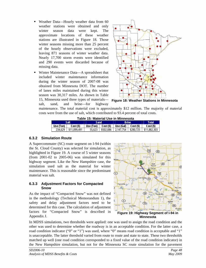
SD2006-10 Page 48 Analysis of MDSS Benefits & Costs May 2009
Weather Data—Hourly weather data from 60 weather stations were obtained and only winter season data were kept. The approximate locations of these weather stations are illustrated in Figure 18. Those winter seasons missing more than 25 percent of the hourly observations were excluded, leaving 871 seasons of winter weather data. Nearly 17,700 storm events were identified and 290 events were discarded because of missing data.
Winter Maintenance Data—A spreadsheet that included winter maintenance information during the winter season of 2007-08 was obtained from Minnesota DOT. The number of lanes miles maintained during this winter season was 30,317 miles. As shown in Table 15, Minnesota used three types of materials—salt, sand, and brine—for highway maintenance. The total material cost is approximately $12 million. The majority of material costs were from the use of salt, which contributed to 93.4 percent of total costs.
Table 15: Material Use in Minnesota Salt Sand Brine Total
Use (Ton) Cost ($) Use (Ton) Cost ($) Use (Gal) Cost ($) Cost ($) 234,629 $11,099,491 55,623 $502,086 2,147,754 $280,725 $11,882,303
6.3.2 Simulation Route A Supercommuter (SC) route segment on I-94 (within the St. Cloud County) was selected for simulation, as highlighted in Figure 19. A course of 5 winter seasons (from 2001-02 to 2005-06) was simulated for this highway segment. Like the New Hampshire case, the simulation used salt as the material for winter maintenance. This is reasonable since the predominant material was salt.
6.3.3 Adjustment Factors for Compacted Snow
As the impact of “Compacted Snow” was not defined in the methodology (Technical Memorandum 1), the safety and delay adjustment factors need to be determined for this case. The calculation of adjustment factors for “Compacted Snow” is described in Appendix J. In MDSS simulations, two thresholds were applied: one was used to assign the road condition and the other was used to determine whether the roadway is in an acceptable condition. For the latter case, a road condition indicator (“0” or “1”) was used, where “0” means road condition is acceptable and “1” is unacceptable. The latter threshold varied from route to route and state to state. These two thresholds matched up well (one road condition corresponded to a fixed value of the road condition indicator) in the New Hampshire simulation, but not for the Minnesota SC route simulation for the pavement
Figure 18: Weather Stations in Minnesota
Figure 19: Highway Segment of I-94 in
Minnesota
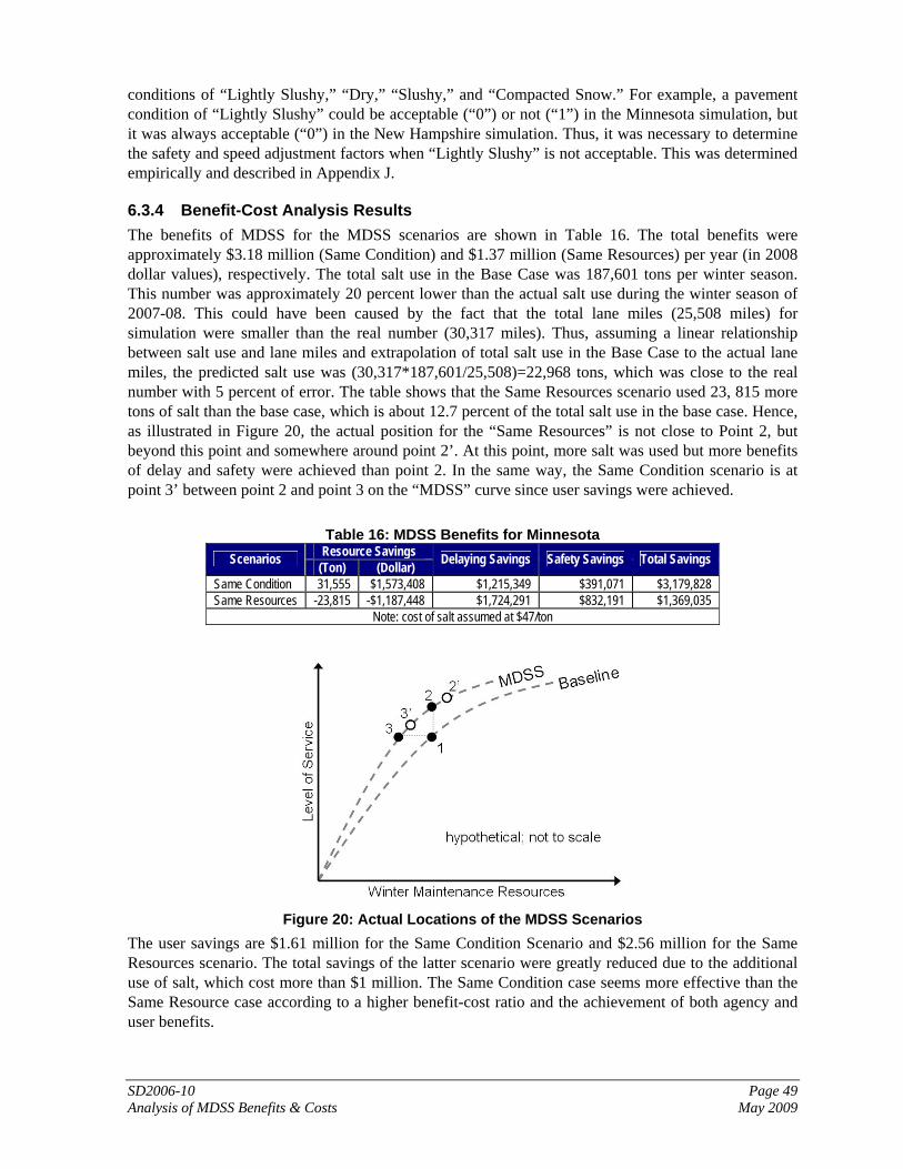
SD2006-10 Page 49 Analysis of MDSS Benefits & Costs May 2009
conditions of “Lightly Slushy,” “Dry,” “Slushy,” and “Compacted Snow.” For example, a pavement condition of “Lightly Slushy” could be acceptable (“0”) or not (“1”) in the Minnesota simulation, but it was always acceptable (“0”) in the New Hampshire simulation. Thus, it was necessary to determine the safety and speed adjustment factors when “Lightly Slushy” is not acceptable. This was determined empirically and described in Appendix J.
6.3.4 Benefit-Cost Analysis Results The benefits of MDSS for the MDSS scenarios are shown in Table 16. The total benefits were approximately $3.18 million (Same Condition) and $1.37 million (Same Resources) per year (in 2008 dollar values), respectively. The total salt use in the Base Case was 187,601 tons per winter season. This number was approximately 20 percent lower than the actual salt use during the winter season of 2007-08. This could have been caused by the fact that the total lane miles (25,508 miles) for simulation were smaller than the real number (30,317 miles). Thus, assuming a linear relationship between salt use and lane miles and extrapolation of total salt use in the Base Case to the actual lane miles, the predicted salt use was (30,317*187,601/25,508)=22,968 tons, which was close to the real number with 5 percent of error. The table shows that the Same Resources scenario used 23, 815 more tons of salt than the base case, which is about 12.7 percent of the total salt use in the base case. Hence, as illustrated in Figure 20, the actual position for the “Same Resources” is not close to Point 2, but beyond this point and somewhere around point 2’. At this point, more salt was used but more benefits of delay and safety were achieved than point 2. In the same way, the Same Condition scenario is at point 3’ between point 2 and point 3 on the “MDSS” curve since user savings were achieved.
Table 16: MDSS Benefits for Minnesota
Resource Savings Scenarios (Ton) (Dollar) Delaying Savings Safety Savings Total Savings
Same Condition 31,555 $1,573,408 $1,215,349 $391,071 $3,179,828 Same Resources -23,815 -$1,187,448 $1,724,291 $832,191 $1,369,035
Note: cost of salt assumed at $47/ton
Figure 20: Actual Locations of the MDSS Scenarios
The user savings are $1.61 million for the Same Condition Scenario and $2.56 million for the Same Resources scenario. The total savings of the latter scenario were greatly reduced due to the additional use of salt, which cost more than $1 million. The Same Condition case seems more effective than the Same Resource case according to a higher benefit-cost ratio and the achievement of both agency and user benefits.
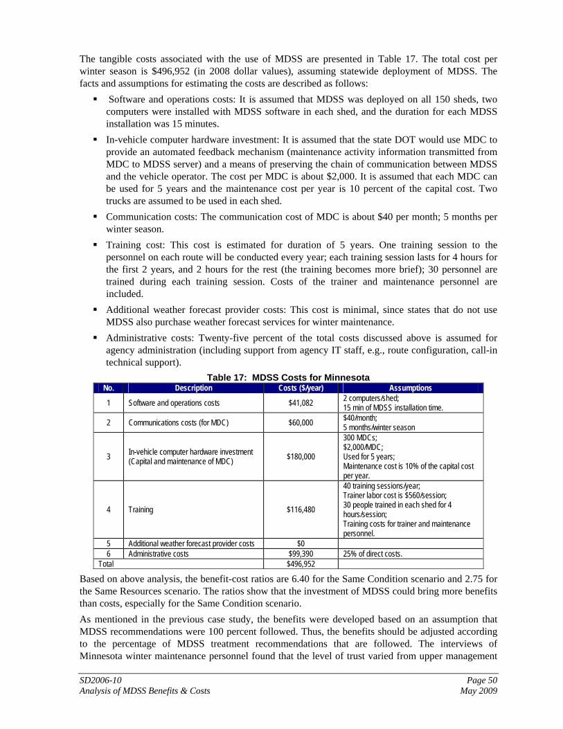
SD2006-10 Page 50 Analysis of MDSS Benefits & Costs May 2009
The tangible costs associated with the use of MDSS are presented in Table 17. The total cost per winter season is $496,952 (in 2008 dollar values), assuming statewide deployment of MDSS. The facts and assumptions for estimating the costs are described as follows:
Software and operations costs: It is assumed that MDSS was deployed on all 150 sheds, two computers were installed with MDSS software in each shed, and the duration for each MDSS installation was 15 minutes.
In-vehicle computer hardware investment: It is assumed that the state DOT would use MDC to provide an automated feedback mechanism (maintenance activity information transmitted from MDC to MDSS server) and a means of preserving the chain of communication between MDSS and the vehicle operator. The cost per MDC is about $2,000. It is assumed that each MDC can be used for 5 years and the maintenance cost per year is 10 percent of the capital cost. Two trucks are assumed to be used in each shed.
Communication costs: The communication cost of MDC is about $40 per month; 5 months per winter season.
Training cost: This cost is estimated for duration of 5 years. One training session to the personnel on each route will be conducted every year; each training session lasts for 4 hours for the first 2 years, and 2 hours for the rest (the training becomes more brief); 30 personnel are trained during each training session. Costs of the trainer and maintenance personnel are included.
Additional weather forecast provider costs: This cost is minimal, since states that do not use MDSS also purchase weather forecast services for winter maintenance.
Administrative costs: Twenty-five percent of the total costs discussed above is assumed for agency administration (including support from agency IT staff, e.g., route configuration, call-in technical support).
Table 17: MDSS Costs for Minnesota No. Description Costs ($/year) Assumptions
1 Software and operations costs $41,082 2 computers/shed; 15 min of MDSS installation time.
2 Communications costs (for MDC) $60,000 $40/month; 5 months/winter season
3 In-vehicle computer hardware investment (Capital and maintenance of MDC) $180,000
300 MDCs; $2,000/MDC; Used for 5 years; Maintenance cost is 10% of the capital cost per year.
4 Training $116,480
40 training sessions/year; Trainer labor cost is $560/session; 30 people trained in each shed for 4 hours/session; Training costs for trainer and maintenance personnel.
5 Additional weather forecast provider costs $0 6 Administrative costs $99,390 25% of direct costs.
Total $496,952
Based on above analysis, the benefit-cost ratios are 6.40 for the Same Condition scenario and 2.75 for the Same Resources scenario. The ratios show that the investment of MDSS could bring more benefits than costs, especially for the Same Condition scenario. As mentioned in the previous case study, the benefits were developed based on an assumption that MDSS recommendations were 100 percent followed. Thus, the benefits should be adjusted according to the percentage of MDSS treatment recommendations that are followed. The interviews of Minnesota winter maintenance personnel found that the level of trust varied from upper management

SD2006-10 Page 51 Analysis of MDSS Benefits & Costs May 2009
(who had less trust) down to the operator. In generally, they would consider all MDSS prescribed treatments that seem reasonable. They felt that the use of MDSS has helped with the timing of treatments and would like to see the technology in the trucks (e.g., MDC, GUI). Because all trucks are assumed to be installed with MDC in the analysis, the percentage of following MDSS recommendations for this case is set to 50 percent. With the assumed percentage, the adjusted benefits are $1,589,913 for the Same Condition scenario and $684,517 for the Same Resources scenario. As a result, the benefit-cost ratios for the MDSS cases are 3.20 and 1.37, respectively.
6.4 Colorado Case Study Stakeholder interviews show that MDSS has been deployed in all 6 Colorado Department of Transportation (CDOT) Regions, but mostly on major highways near Aspen, Glenwood Springs, and Colorado Springs to Denver and full deployment in Region 4 (northeast Colorado on major highways). This case study used an interstate highway segment in Aurora, Colorado for simulation to support the statewide benefit-cost analysis.
6.4.1 Baseline Data The data for developing the baseline data module are described as follows:
Road Data—To develop baseline route segment information, two data files were gathered: a Microsoft Access file for maintenance highway segment and a GIS shapefile. The Access file included the name of the highway segment, highway number, starting and ending mileposts, and other information. The GIS shapefile contained the name of route, starting and ending reference points, segment length, location, and so on. A highway segment in the Access file consists of one or more consecutive segments in the shapefile in terms of starting and ending points. Thus, these consecutive segments in the shapefile were aggregated to generate the corresponding segment information in the Access file. The method of aggregation (e.g., for AADT, speed limit) is similar to that described in the New Hampshire case study. As a result, the baseline data module included 613 highway segments on 282 highways, which covered 9,057 centerline miles (equal to 19,676 lane miles by assuming 4 vehicle lanes on interstate highways and 2 lanes on others).
Crash Data—Four winter seasons (from 2000-01 to 2003-04) of crash data were obtained. The crash datasheet included the location of crash (highway name, milepost), crash severity (e.g., fatality, injury, or property damage only [PDO]), date and time, pavement condition, lighting, weather, and other information. The crash data were mapped to the highway segments in the baseline module. The number of crashes for each highway segment was calculated for each winter season. The average value for these four winter seasons was used to estimate an average crash rate. The total numbers of fatalities, injuries, and PDOs during these winter seasons were calculated to estimate the average accident cost, which resulted in $37,000 per crash (2008 dollar values).
Traffic Volume Data—Another GIS shapefile that contained AADT data for the years of 2005 and 2006 were obtained. This file included information of route segment, starting and ending points, AADT, truck percentage, and so on. To calculate the winter truck and non-truck AADT, a statewide seasonal adjustment factor was developed based on monthly data collected from 108 ATR stations for the years of 2005 and 2006. The average adjustment factor (0.891) was used and applied to all route segments to calculate winter truck and non-truck ADT.
Weather Data—Hourly weather data from over 30 weather stations were obtained and only winter season data were used for developing the baseline data module. Those winter seasons missing more than 25 percent of the hourly observations were excluded, leaving 431 seasons of winter weather data. 10,461 storm events were identified and 224 events were discarded
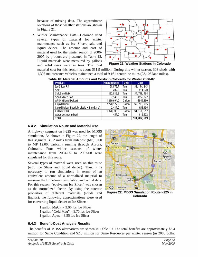
SD2006-10 Page 52 Analysis of MDSS Benefits & Costs May 2009
because of missing data. The approximate locations of those weather stations are shown in Figure 21.
Winter Maintenance Data—Colorado used several types of material for winter maintenance such as Ice Slicer, salt, and liquid deicer. The amount and cost of material used for the winter season of 2006-2007 by product are presented in Table 18. Liquid materials were measured by gallons and solid ones were in tons. The total material cost for this season is about $11.9 million. During this winter season, 303 sheds with 1,393 maintenance vehicles maintained a total of 9,161 centerline miles (23,106 lane miles).
Table 18: Material Amounts and Costs in Colorado for Winter 2006-07 Product Amount Used Unit Cost Ice Slicer RS 28,875.7 Ton $2, 194, 243 Salt 492.0 Ton $14,570 Salt/Sand Mix 192,815.3 Ton $4, 718, 464 Sand Slicer - ton 7,145.0 Ton $155,272 APEX (Liquid Deicer) 1,250,694.0 Gallon $849,830 Liquid Deicer 7,270,127.0 Gallon $2, 733, 995 Liquid Deicer Special ( Liquid + Salt/Sand) 2,417.0 Ton $53,196 Caliber 1000 1,870,393.0 Gallon $1, 160, 517 Abrasives non-mixed 457.0 Ton $12,502 Total $11, 892, 589
6.4.2 Simulation Route and Material Use A highway segment on I-225 was used for MDSS simulation. As shown in Figure 22, the length of this segment is 12 miles from milepost (MP) 0.00 to MP 12.00, basically running through Aurora, Colorado. Four winter seasons of winter maintenance from 2004-05 to 2007-08 were simulated for this route. Several types of material were used on this route (e.g., Ice Slicer and liquid deicer). Thus, it is necessary to run simulations in terms of an equivalent amount of a normalized material to measure the fit between simulation and actual data. For this reason, “equivalent Ice Slicer” was chosen as the normalized factor. By using the eutectic properties of different materials (solids and liquids), the following approximations were used for converting liquid deicer to Ice Slicer:
1 gallon MgCl2 = 2.96 lbs Ice Slicer 1 gallon “Cold Mag” = 3.75 lbs Ice Slicer 1 gallon Apex = 3.55 lbs Ice Slicer
6.4.3 Benefit-Cost Analysis Results The benefits of MDSS alternatives are shown in Table 19. The total benefits are approximately $3.4 million for Same Condition and $2.0 million for Same Resources per winter season (in 2008 dollar
Figure 21: Weather Stations in Colorado
Figure 22: MDSS Simulation Route I-225 in
Colorado

SD2006-10 Page 53 Analysis of MDSS Benefits & Costs May 2009
values). The total Ice Slicer use in the Base Case is 107,091 tons per winter season. The difference of Ice Slicer use between the Same Resources scenario and the Base Case is 2,007 tons, which is equal to 1.9 percent of the total use in the Base Case. CDOT used almost 10 types of materials for winter maintenance. To compare the total material use between the Base Case and the actual data, the various types of materials need to be converted to an equivalent material, which is Ice Slicer. The conversion is conducted by different ways for liquid and solid materials. For solid materials of salt, salt/sand mix, sand slicer, liquid + salt/sand, and abrasive non-mixed, the equivalent use of Ice Slicer is calculated based on unit prices ($/ton). For example, the cost of Ice Slicer is ($2,194,243/28,875.7=) $75.99/ton, then the 492 tons of salt is equivalent to (14,570/75.99=) 191.7 tons of Ice Slicer. For liquid materials, the equivalent factors are obtained from those used for simulation. One gallon of Apex (liquid deicer) is equivalent to 3.55 lbs of Ice Slicer; for liquid deicer and Caliber 1000, one gallon of liquid corresponds to ((2.96+ 3.75)/2=) 3.36 lbs of Ice Slicer for simplicity. After the normalization of materials, the total use of equivalent Ice Slicer during the winter season is 111,622 tons, which is about 4,531 tons more than the Base Case. However, the numbers of lane miles for the Base Case and the real data are different (19,676 and 23,106 miles respectively). Assuming that resource use is proportional to lane miles, the total use in the Base Case increases to 125,759 tons, which is 14,138 tons more than the actual data. This is reasonable since the highway route for simulation is an interstate highway segment with relatively high AADT, and thus required more resources to keep a higher level of service than other lower class routes during winter events.
Table 19: MDSS Benefits for Colorado
Resource Savings Scenarios (Ton) (Dollar) Delaying Savings Safety Savings Total Savings
Same Condition 21,435 $1,728,292 $563,987 $1,075,530 $3,367,810 Same Resources 2,007 $161,790 $557,055 $1,226,224 $1,985,069
Note: cost of Ice Slicer assumed at $76/ton.
Table 19 also shows that user benefits (delay and safety) for the MDSS scenarios are $1.63 million (Same Condition) and $1.78 million (Same Resources). The achievement of user benefits from Same Condition to Same Resources is less than $0.2 million, which means that the extra use of Ice Slicer in the Same Resources scenario did not improve pavement conditions a lot over the Same Condition scenario. This implies that the Same Condition scenario is preferable for this case. After examining output data from the simulation, the user savings of the Same Condition scenario stemmed from the improvement of pavement conditions, e.g., compacted snow (Base Case) lightly slushy (Same Condition). Although 21,435 tons of Ice Slicer were saved in the Same Condition scenario, user benefits were still achieved through using better maintenance treatments (e.g., application time and rate of materials). The tangible costs per winter season are presented in Table 20. The total costs per winter season with the use of MDSS are approximately $1.5 million (in 2008 dollar values), assuming statewide deployment of MDSS. The facts and assumptions for estimating the costs are described as follows:
Software and operations costs: It was assumed that MDSS was deployed on all 307 maintenance sheds, two computers were installed with MDSS software in each shed, and the duration for each MDSS installation was 15 minutes.
In-vehicle computer hardware investment: It was assumed that the state DOT would use MDC to provide an automated feedback mechanism (maintenance activity information transmitted from MDC to MDSS server) and a means of preserving the chain of communication between MDSS and the vehicle operator. The cost per MDC is about $2,000. It was assumed that each MDC can be used for 5 years, and the maintenance cost per year is 10 percent of the capital cost. In total 1,393 MDCs were installed in trucks.

SD2006-10 Page 54 Analysis of MDSS Benefits & Costs May 2009
Communications costs: The communications cost of MDC is about $40 per month; 5 months per winter season.
Training cost: This cost is estimated for a period of 5 years. One training session to the personnel on each route will be conducted every year; each training session lasts for 4 hours for the first 2 years, and 2 hours for the rest (the training becomes more brief); 5 operators were trained per shed, with a total of 1535 people trained. Costs of the trainer and maintenance personnel are included.
Additional weather forecast provider costs: This cost is minimal, since states that do not use MDSS also purchase weather forecast services for winter maintenance.
Administrative costs: Ten percent of the direct costs ($1.4 million) was used for agency administration (including support from agency IT staff, e.g., route configuration, call-in technical support). The reason that 10 percent was used instead of 25 percent (in the previous two cases) is because the majority (80 percent) of the direct costs is from computer hardware investment and associated communications costs.
Table 20: MDSS Costs for Colorado No. Description Costs ($/year) Assumptions
1 Software and operations costs $76,406 307 sheds; 2 computers/shed; 15 min of MDSS installation time.
2 Communications costs (for MDC) $278,600 $40/month; 5 months/winter season
3 In-vehicle computer hardware investment (Capital and maintenance of MDC) $835,800
1393 trucks; 1 MDC on each truck; $2,000/MDC; Used for 5 years; Maintenance cost is 10% of the capital cost per year.
4 Training $163,324 5 operator trained in each shed for 4 hours; Training costs for trainer and maintenance personnel.
5 Additional weather forecast provider costs $0 6 Administrative costs $136,181 10% of direct costs.
Total $1,497,985
The tangible benefits and costs associated with the use of MDSS result in benefit-cost ratios of 2.25 for the Same Condition scenario and 1.33 for the Same Resources scenario. Thus, the investment returns are 125 percent and 33 percent of the costs, respectively. Stakeholder interviews show that maintenance personnel generally trusted MDSS recommendations. They perceived MDSS-prescribed treatments as guidance; some felt MDSS may be used as directive one day with increased trust. They generally believed that MDSS has helped to increase safety, mobility, and aided in cost savings. Thus, if it is assumed that 75 percent of MDSS recommendations are followed by maintenance operators in this state, the benefits of the MDSS scenarios become $2.5 million (Same Condition) and $1.5 million (Same Resource). The corresponding benefit-cost ratios are 1.69 and 0.99, respectively. The Same Condition scenario still has investment return of 69 percent of the costs, while the costs and benefits are almost the same for the Same Resources scenario.
6.5 Summary The analysis results of benefits and costs for the three case studies are summarized in Table 21. The results show that the use of MDSS for winter maintenance could bring more benefits than costs. However, the benefit-cost ratios vary with cases: 2.25–7.11 for the Same Condition scenario and 1.33 – 8.67 for the Same Resources scenario. For the Same Condition scenario, it is found that the contributions of user benefits to total benefits are almost the same as agency benefits for all cases. The splits of benefits for the Same Resources scenario, however, have large variations. In the Minnesota case, the Same Resources scenario used much more salt (12.7 percent of total use) than the Base Case

SD2006-10 Page 55 Analysis of MDSS Benefits & Costs May 2009
for winter maintenance and seemed to deviate more from the assumed “Same Resources” point 2 (in Figure 12) than the other two cases. The additional use of salt did improve motorist safety and mobility, but the total benefits were reduced. By comparing benefit-cost ratios, the Same Condition scenario tends to produce similar or better results than the Same Resources scenario.
Table 21: Summary of Benefit-Cost Analysis
Case State Scenario Benefits Percent of User
Savings (%) Percent of Agency
Savings (%) Costs B-C Ratio Same Condition $2,367,409 50 50 7.11 New
Hampshire Same Resources $2,884,904 99 1 $332,879
8.67
Same Condition $3,179,828 51 49 6.40 Minnesota
Same Resources $1,369,035 187 -87 $496,952
2.75
Same Condition $3,367,810 49 51 2.25 Colorado
Same Resources $1,985,069 90 10 $1,497,985
1.33

SD2006-10 Page 56 Analysis of MDSS Benefits & Costs May 2009
7. ANALYSIS OF INTANGIBLE BENEFITS AND COSTS This study incorporates FHWA’s benefit-cost analysis guidelines of three groups (agency costs, user costs and benefits, and non-user impacts) as investment costs, operational costs and benefits, and externalities. The intangible benefits and intangible costs identified within the operational and externality groups through this analysis of the Pooled fund (PF) MDSS are presented in this section. These qualitative “spin-off” benefits of the PF-MDSS deployment are discussed and characterized using the system’s objectives and their supporting functions. Function analysis is used to provide a characterization framework. Characterizations of the intangible benefits of individual functions of the PF-MDSS are supported with anecdotal observations from the interviews conducted as part of this research project.
7.1 Intangible Benefits and Costs Defined Intangible benefits and costs are the ones that are theorized to be present based on various logical arguments, observations, and experiences. They are often qualitative and resultant of loose or overlapping connections (spin-offs). Attaching monetary values to intangibles is difficult as a result of the following common qualities.
They lack the common unit of measurement applied to the tangible ones. They often are described in terms of value, of which the estimation is a key source of analysis
inaccuracies. Though intangible, they still affect customer choices and satisfaction. Ultimately, an agency must rely on its corporate culture to assess the value of intangible
benefits. Keen (25) defined decision support systems as interactive systems “designed to help improve the effectiveness and productivity of managers and professionals.” He identified a range of functional areas and types of tasks including the following common features:
“They are non-routine and involve frequent ad hoc analysis, fast access to data, and generation of non-standard reports”
“They often address ‘what if?’ questions” “They have no obvious correct answers; the manager has to make qualitative tradeoffs and take
into account situational factors.” In the simplest sense, decision support systems provide fundamentally intangible benefits as described by Keen (26). He provides a set of decision support system benefit examples frequently cited in earlier case studies.
increase in number of alternatives examined
better understanding of the business fast response to unexpected situations ability to carry out ad hoc analysis new insights and learning improved communication
control cost savings better decisions more effective teamwork time savings making better use of data resources
Of these, only cost and time savings can be tracked to a straightforward cost / benefit analysis. The use of performance measures is an attempt to quantify the outcomes of winter maintenance activities. The PF-MDSS in itself is an attempt to quantify the application of rules of practice to weather prediction. As such, representative quantitative performance measures were adoptable in the tangible benefit

SD2006-10 Page 57 Analysis of MDSS Benefits & Costs May 2009
analysis. However, if one takes the definition of intangible as an aspect of the product or outcome of a service offering that has a value but is difficult to see or quantify, many of the informal winter maintenance goals of the investigated states can be described as intangible benefits (Table 22).
Table 22: Winter Maintenance Goals Taken from Interview Notes and Transcriptions and Illustrating Their Intangible Nature
State Maintenance Goals Colorado to keep the roads “clear and safe as possible throughout the state.” Indiana aimed at “getting back to bare pavement as quickly as possible.”
Iowa work very hard to keep the roads clear and drivable at all times Kansas keep the roads safe and open at all times.
Minnesota clear roads and mobility with strong consideration of cost-effectiveness New Hampshire “aggressive” efforts to keep roads open
North Dakota “seamless boundaries” and “continuous levels of service.” South Dakota “to provide the best possible winter driving conditions… with what we have for equipment and manpower.”
Wyoming “to keep Interstate 80 traffic flowing. That’s our number one priority.” Throughout the following discussion of intangible benefits and costs, it will be clear that many of the intangible benefits gained through the application of the PF-MDSS result from an integrative HCI (human computer interface), the incorporation of a quantitative technology platform with the ability to compare activity alternatives, and the required collection, documentation, and inputs of quantitative performance definitions and metrics. Intangible costs are subtle and for the purposes of this study are taken to be those that are hidden in larger budgets, buried in ordinary operating expenses, or camouflage existing activities. Characteristically, they affect individuals and society in the long run. For example the time it takes to do clerical and technical tasks such as ordering, installing, and securing hardware and software usually supersede time doing existing tasks.
7.2 MDSS Function Analysis The stated objective of an MDSS is to provide support (through software systems) for proactive maintenance decision making before and during adverse weather events, with use resulting in a higher level of service, reduced operational costs, and/or safer highway conditions. The framework for the analysis of the operational intangibles is that of the functions performed by the PF-MDSS to meet the objective. This recognition of functions as the benefit-producing core of MDSS was expressed in the client’s requested task to describe the essential functions of a winter MDSS. In the end, a benefit-cost analysis strives to determine whether benefits outweigh costs at an acceptable ratio. Another perspective of this is determining whether costs are too high for the function proposed to supply the customer with what the customer desires. The first step in identifying functions is to determine the purpose of the system. Meridian's MDSS meets the objective described above with a "one-stop-shop" theme of merging weather, maintenance, and RWIS data into a unified visualization and decision support tool in order to realize the maximum benefit. For this project, the defined purpose of the PF-MDSS is to:
Predict and portray how road conditions will change due to the forecast weather and the application of several candidate road maintenance treatments.
Suggest optimal maintenance treatments that can be achieved within available staffing, equipment, and materials resources.
Accomplish in-situ integration of primary and secondary functions essential to winter maintenance.
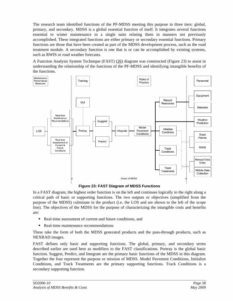
SD2006-10 Page 58 Analysis of MDSS Benefits & Costs May 2009
The research team identified functions of the PF-MDSS meeting this purpose in three tiers: global, primary, and secondary. MDSS is a global essential function of itself. It integrates several functions essential to winter maintenance in a single suite relating them in manners not previously accomplished. These integrated functions are either primary or secondary essential functions. Primary functions are those that have been created as part of the MDSS development process, such as the road treatment module. A secondary function is one that is or can be accomplished by existing systems, such as RWIS or road weather forecasts. A Function Analysis System Technique (FAST) (26) diagram was constructed (Figure 23) to assist in understanding the relationship of the functions of the PF-MDSS and identifying intangible benefits of the functions.
Figure 23: FAST Diagram of MDSS Functions
In a FAST diagram, the highest order function is on the left and continues logically to the right along a critical path of basic or supporting functions. The two outputs or objectives (simplified from the purpose of the MDSS) culminate in the product (i.e. the LOS and are shown to the left of the scope line). The objectives of the MDSS for the purpose of characterizing the intangible costs and benefits are:
Real-time assessment of current and future conditions, and Real-time maintenance recommendations
These take the form of both the MDSS generated products and the pass-through products, such as NEXRAD images. FAST defines only basic and supporting functions. The global, primary, and secondary terms described earlier are used here as modifiers to the FAST classifications. Portray is the global basic function. Suggest, Predict, and Integrate are the primary basic functions of the MDSS in this diagram. Together the four represent the purpose or mission of MDSS. Model Pavement Conditions, Initialize Conditions, and Track Treatments are the primary supporting functions. Track Conditions is a secondary supporting function.

SD2006-10 Page 59 Analysis of MDSS Benefits & Costs May 2009
Darker lines indicate primary connections along the critical path. The fork style path to the left of the function Record Resources indicates that both Equipment AND Materials are supporting functions. The fork style path to the left of the function Track Treatments represents Manual Data Entry OR Mobile Data Collection” as supporting functions. The dashed line boxes at the top represent specifications or particular parameters that must be achieved to satisfy the function(s).
7.3 Intangible Benefits by MDSS Function A component of this study was interviews conducted with the supervisory and operational personnel directly related to that state’s deployment of the PF-MDSS (see Section 4). For this section, the results of those interviews were reviewed in light of the identification of MDSS functional analysis. Notes and quotes of the interviewees are presented here where they highlight benefits experienced by the supervisors and personnel from the states involved in the PF-MDSS test. Additional supporting comments addressing the Meridian side of the functions were taken from various Pooled Fund documents and reports. Interestingly, comments associated with highest order functions (closer to the left of the FAST diagram) focus on what is familiar (e.g. RADAR or RWIS); improved access (Internet distributed and in-vehicle); and unrealized supporting functions (e.g. MDC).
7.3.1 Portray The Portray function is regularly the primary function in descriptions of the PF-MDSS use and potential. This function uses the GUI to present the results of the other basic functions, portrayal of the treatment alternatives and prediction of the associated pavement conditions. The portrayal of information at the user level is often considered “to be the MDSS” as evidenced in the following interview excerpts. This perception of MDSS by many of the interviewees is supported by the positional isolation of Portray as the highest order function within the PF-MDSS. Several of these supervisors are anxious to have it [MDSS] in their own work vehicles:
“I have even got it on my computer at home so I am constantly watching it.” (Colorado) “I’ve got MDSS units on each of my computers, where I can pull it up at anytime… With the MDSS, I can track the weather … I don’t think you can actually beat it for tracking the winds and stuff like that; it’s an excellent tool.” (Indiana) “What I like about it is it is all in one place, I can look at radar, I can look at RWIS, AWAS system, pavement temperatures, visibility, [and] dew points. [MDSS] is pretty much a one-stop shop for me, instead of bouncing around to all of these different places I can go to one place and see what I need to see.” (Iowa) “On our MDSS routes, we have the IWAPI system so our trucks have almost real-time information… we are giving them a radar picture now as well as an updated short term forecast from MDSS and the guys that have that really like it.” (Kansas) “That is why I am pushing to move to MDSS, because I have too much information to look at to make a good decision.” (Minnesota)
One aspect of the MDSS forecasting capabilities that has been well received is the integration of weather information:
“It’s really a one-stop shop – pull the cameras, pull the RWIS. I think the biggest advantage is how the program is able to run projections (radar, snowfalls), it’s nice to know what you need to expect, 4 inches or 12 inches and when that’s going to come.” (Wyoming)

SD2006-10 Page 60 Analysis of MDSS Benefits & Costs May 2009
Meridian’s Draft Phase IV Interim Report included findings that describe intangible benefits of the Portray function:
The use of MDSS as an information portal for supporting maintenance decisions should not be understated relative to its role in making explicit maintenance recommendations. Many users initially adopt MDSS as a dynamic situation display and slowly transition to more frequent adoption of the recommendations it makes. (27)
7.3.2 Predict / Suggest The Predict conditions and Suggest treatment alternative functions represent the heart of the PF-MDSS and are co-critical, i.e. the MDSS would not be a decision support system without both. These two primary basic functions are positioned equally important along the critical path and are discussed together. Comments by the participating personnel illustrate a positive effect of the intangible benefits on the present operational culture. They reflect shifts that affect future circumstances.
“I think [MDSS] changes [practices], it gives us an idea, it questions us. If MDSS says we can do it with 200 lbs and not 300 or 400 lbs, do we really need that? I think that’s what we’re all striving for with MDSS, you know, if we are doing too much overtreating. That’s what we want to know.” (Iowa)
One supervisor estimated that MDSS use is producing a 10% savings in the winter maintenance budget through reductions in staffing hours and equipment hours, because
“It lets us put the right material at the right place, with the manpower at the right time.” (Iowa) While respondents are not able to quantify benefits yet, nearly all said that they believe it is helping them look at application rates more critically, and that it will eventually lead to savings in materials:
“I think it has made us more efficient and aware…when we started out we were just going out and making sure we covered our whole route, whether we were using salt or salt/sand…I think we are changing that, by using salt only in extreme cold and by looking at the cost of what we are putting out there.” (Indiana)
Respondents generally trust the recommendations in principle, and think that MDSS is very helpful with the timing of treatments. Long-term, respondents believe that MDSS has the potential to help them look at application rates more critically, leading to savings in materials.
“[Now] we just try to get to the level of service, but not in the most economical way. There are a lot of alternate chemicals out there people want to try and are trying, and some of them are grossly expensive, but there may be a window of opportunity where they are very effective, but they are just used in a blanket and we are wasting a ton of money. ” (Minnesota) “For years we just went and plowed. With MDSS it gives application rates, and the new guys, it helps in getting those guys up to speed on what it is we are trying to accomplish, out there when we go to spread our materials, whether it be just our regular salting and abrasive materials or the IceSlicer and chemicals.” (Wyoming)
7.3.3 Integrate Integrating supporting functions is a primary basic function of the PF-MDSS. This stage along the critical path represents the blending of several supporting functions. It is an invisible function, hence there were no interview comments. Those that did mention “integration” described ensemble weather forecasting rather than integration of the components and sources of information within the PF-MDSS. This is evident in the following interview excerpt, which is relating the Weather Prediction supporting function outside the scope of the MDSS.
SD2006-10 Page 61 Analysis of MDSS Benefits & Costs May 2009
Respondents consistently praised the weather and forecasting features of MDSS, citing the depth of information (“it carries more information on it than anything else”), and in particular how it integrates information from various sources. “Instead of just giving you one forecast and the models, they will take 20 forecasts and throw them into a computer, weight them based on which one has been more right than that one, and put one big forecast with 20 different little forecasts as input.” (Iowa)
7.3.4 Model Pavement Condition Model Pavement Condition is a primary supporting function that was created as part of the MDSS development process. It is very different from the type of pavement forecast commonly associated with RWIS to which personnel have been accustomed. This function represents the greatest intangible benefit along with the greatest departure from previous winter maintenance planning and decision-making. Comments from the interviews provide insight into the early stage of adoption. Winter maintenance personnel are highly risk adverse when they know a strategy or treatment historically works for them. All have experience with unfavorable outcomes of trying something new or cutting back on application rates they know to be effective. This theme is a thread through the comments provided here.
“Initially they were like, ‘uhhh I don’t know,’ and we kept talking back and forth and they decided they would start following the recommendations, and every time something didn’t work…[they would say] ‘this isn’t good.’ And by the end of the season it was working beautifully…and they were following the recommendations even to the point where in the past we wouldn’t have followed the recommendation that we tried with MDSS, and we had great success.” (Colorado)
In terms of using MDSS for anti-icing/deicing treatment, all respondents regard the treatment recommendations as guidance and not directives. Respondents generally trust the recommendations in principle, and think that MDSS is very helpful with the timing of treatments. However, most respondents said that the application rates recommended are revised based on driver experience, site-specific conditions, or resource issues:
“MDSS would recommend at times 1,000 lbs per lane mile, but you can’t do that with the equipment the truck structurally has.” One respondent estimated that his sub-district followed the treatment recommendations “about 80% of the time.” (Indiana)
By contrast, respondents do not appear to have a great deal of confidence in the MDSS treatment recommendations. While all respondents stated that they look at and consider the recommendations, they do not follow them with frequency. (One respondent stated that he followed them only 5% of the time). Reasons for not following the recommendations ranged from resource constraints (“sometimes crews are not available”) to past experience with inaccurate recommendations (“at first the recommendations were really high, which were way more than we actually use, and then they went the other way and went too low.”). There also appears to be institutional resistance to not plowing the roads when there is snow on the ground: “Any time we’re out and we have got snow on the ground we plow, and sometimes MDSS says we don’t have to plow and I just don’t see that happening.” When asked if they trusted the treatment recommendations, three of the four respondents answered “no.” (Iowa) While the representatives view the MDSS treatment recommendations as guidance and not directive, the level of trust in MDSS appears to be very high, with one participant responding that they follow the MDSS recommendations “nearly always now” at the Dodge City site. Trust issues are more directly related to forecast accuracy. (Kansas) Most respondents said that the application rates are not regularly followed yet, because MDSS tends to recommend lower application rates than MnDOT has traditionally used. (Minnesota)
SD2006-10 Page 62 Analysis of MDSS Benefits & Costs May 2009
In terms of using MDSS for anti-icing/deicing treatment, all respondents regard the treatment recommendations as guidance and not directives. All respondents consult the MDSS recommendations, and several use it to run scenarios on more than one treatment option. Many indicated a high level of willingness to try the recommendations whenever possible:
“I try to use the amount of treatment MDSS tells me to use,” and, “With my experience with MDSS so far, I would absolutely trust it and I would do it.” (North Dakota)
Intangible benefits include ideas and observations that are loosely related to the task but resultant from considering or practicing it. Many of the comments and discussions over the course of this project clearly identify the vital role of judgement and its value in winter maintenance through the testing and deployment of the PF-MDSS. Several reasons were given for why MDSS treatment recommendations are not always followed: forecasts, resources, and personal experience. In terms of forecasts, several respondents commented that if they note that the MDSS forecast for a specific location is inaccurate, they are not inclined to follow the treatment recommendations. Finally, some operators use MDSS as initial guidance, but tend to adapt it based on personal experience and field conditions:
“Do I trust it? Sure I’ll trust it that’s not a problem. Do I totally follow what they’re saying? Depends on what the lines are telling me. You take it into consideration and then you get out on the field and take a look and see what you’ve got…. I’ve got to rely on myself and my eyes.” (North Dakota)
Meridian’s Draft Phase IV Interim Report included astute observations on this role of judgement in their discussion of human factors relating to the PF-MDSS test.
Decisions need to be made as to where the line lies between science and judgment. For example, if an icy road can be brought back into specifications immediately while working within the maintenance resource constraints configured for that road, should MDSS ever consider leaving the road icy in favor of resolving the problem with fewer resources at some later time. To make this type of decision MDSS would need information that is presently lacking on how to weigh risks to the public vs. savings to the agency in making such decisions. (28)
There is high potential for intangible benefit of MDSS deployment if deployed on a key statewide route basis. The results of the Model Pavement Conditions as presented in Predict and Suggest can be used in decision support of the adjacent maintenance segments for a given station without the deployment costs of defining the parameters for those segments. It is an observation by the project team that this speaks to a potential improvement to the Predict/Suggest/Portray function of the MDSS. If uncertainty error bars of the prediction were presented in a front-line context rather than the result of changing parameters in a ‘what if scenario’; the system could provide better decision support. To the user this could take a form such as “increasing the snowfall rate from the predicted of 1 inch per hour to 1½ inch per hour will require an additional 100 lbs per lane mile application rate.”
7.3.5 Track Pavement Conditions / Initialize [Model] Conditions The FAST diagram shows both Track Pavement Conditions AND Initialize Conditions for the pavement condition model being support by Road Patrols OR RWIS. This represents an option for automated or manual input to the MDSS. The development of new technology that at some level relies on existing outside systems often reveals new insights and understandings of limits and benefits of the existing system. The PF-MDSS was not immune to this. Meridian’s efforts resulted in the following finding specific to this function as an example of this.

SD2006-10 Page 63 Analysis of MDSS Benefits & Costs May 2009
Real-time winter weather observation capabilities [for blowing snow and snow precipitation] are seriously lacking, and these limitations can substantially degrade the ability of MDSS to track the real-time situation occurring on an agency’s road network. Winter precipitation observations are especially lacking. Even where they are presently available, the accuracy of these observations is often suspected. (28)
7.3.6 Track Treatments The Track Treatments function is supported by either Manual Data Entry OR Mobile Data Collection (MDC). Maintenance data reporting is a key issue, since a lot of value is lost without it. MDC outputs are where (location of vehicle, correlated to route segment) and what (whether plowing or not, the plow lane, whether spreading or not, the spreading lane, the material type, and rate). Options include speed and direction of travel, use of additional plow blades, and road and weather conditions. The Track Treatments function was highly underused during the operational use of the PF-MDSS. This function played a key role in the simulation analysis, which assumed that all treatment recommendations were followed. The major intangible benefit role of this function was identified through the simulation and emphasized the value of MDC as a supporting function to MDSS. This is evident in the crucial reliance of the Suggest/Predict functions on the interactions and instances of timeliness or appropriate granularity of treatments and resource use information. Other identified intangible benefits include:
better recording of actual maintenance actions supported by MDC the ability to make mid-course corrections to improve storm response suggested by MDSS with
MDC support the ability to have data to support performance measurement and review of maintenance actions
and decisions. The intangible benefits stood out in the interviews:
Winter maintenance managers encourage use of the treatment recommendations as much as possible. They also enter as much information into the system as possible, so that the treatment recommendations reflect state rules of practice, past treatments, and products available at the shed. (Colorado)
Nearly all supervisors stated that operators who make changes are supposed to notify their supervisors regarding the change: “If they’re changing the rate I can dial into MDSS and put the rate they’re using into MDSS and decide if it’s going to work or not.” (North Dakota)
Meridian’s findings solidly supported the intangible benefit of this function when combined with the MDC supporting function. While proven to be technologically possible, the PFS MDSS demonstration tests have shown that automated reporting of maintenance activities is much more promising than manual reporting. (28) A true time-savings benefit could be calculated for the contribution of MDC to this intangible, given the hourly requirement and wage accomplishing this function through the operational day. A separate cost benefit analysis of MDC would be reasonable.
7.3.7 Record Resources The Record Resources function was identified as a supporting function in the FAST. The MDSS has the capability to record and use constrained resources. Treatment recommendations are made by the MDSS in light of road weather scenarios as well as resource constraints. However, interviews of some states suggest that there is a need to further improve this function, by taking into account not only materials availability but also staffing, equipment, and infrastructure constraints:
SD2006-10 Page 64 Analysis of MDSS Benefits & Costs May 2009
“MDSS may be telling us this activity is going to occur and we may not have the manpower or equipment to follow these recommendations.” (South Dakota) “We don’t have adequate storage [for salt] in all of our sections, so … we can’t use sometimes the best option that MDSS suggests because we don’t have the infrastructure or equipment in place.” (North Dakota)
It is an observation by the project team that a potential improvement of the PF-MDSS can be realized through the inclusion of additional operational rules of practice. These may take the form of geographical and inventory logic to resources (e.g. “this is an out and back route with 2 trucks available, 1 with 10 cubic yards, the second 8 cubic yards” or “this is a one way route with X amount of material at the end.”).
7.4 Intangible Benefits from Function Specifications in MDSS Across the top of the FAST diagram are three dash line boxes that represent specifications or particular parameters that must be achieved to satisfy the function(s) of the MDSS. These include Maintenance Performance Measures, Training, and Rules of Practice. The relationship these have with the implementation and operation of the MDSS provides insight and/or areas of improvement for each. This is an intangible benefit of the PF-MDSS.
7.4.1 Maintenance Performance Measures Fundamental to the cost / benefit analysis was the establishment of metrics that could be used in the tangibles analysis. This provided the opportunity to look closely at what constituted meeting the goal level of service and “forced” a quantitative valuation of such. Two very different performance measures were evaluated through the simulation: road condition change and deicer quantity use. Quantification of a LOS for the simulation methodology resulted in potential intangible benefits. An example of such can be found in Meridian’s discussion of CDOT’s deicer use and suggestion that it may be difficult for MDSS to save deicer without changing the intent of that deicer. That a performance measure may be just to improve the pavement condition of the road using ~X lbs of salt, not necessarily to achieve a specific condition. The technology platform of the PF-MDSS has the potential to make performance measure easier. With the basic technology infrastructure, it can increase the capability and effectiveness of winter maintenance operations through the addition of other technologies such as MDC.
7.4.2 Training Proponents often tout the value associated with use of the MDSS for training. Support for this was evident throughout the different state responses. Highway snow and ice control has become a complex task. Dörner (28) systematically evaluated the processes of why complex decision making processes fail. He concludes that simulation for gaining experience in making decisions under complex situations is one of the few chances of avoiding mistakes when the decisions are made for real. The intangible benefit of both training to use the PF-MDSS and using the PF-MDSS to train come through clearly in the interviews. Several respondents also view MDSS as an effective training tool: for management to consider “what-if” scenarios during exercises, as well as for foreman and vehicle drivers who will be making treatment decisions.
“If it’s a new guy, it’s something he can use to become familiar with events, and give him a little bit more of a basis for the decisions he’s making. And if it’s a veteran to use more of the “what ifs”; he may be a little bit more proactive or feel a little more confident in trying new things.” (Indiana)

SD2006-10 Page 65 Analysis of MDSS Benefits & Costs May 2009
The participants can foresee other future benefits. Several respondents mentioned its potential as an effective training tool:
“One of my expectations was that if [operators] needed a recommendation on how to treat a road, [they] could get guidance without a supervisor having to coach them.” (Iowa) “I have been here 18 years and experience is a big factor, but MDSS is a good tool to help the experience I believe.” (Minnesota)
7.4.3 Rules of Practice The Rules of Practice define the actions that are recommended by the MDSS to meet specific performance measures. Through the application of the MDSS, outcomes of changes in rules of practice can be compared against unchanged rules. The successful simulation use of the PF-MDSS illustrates an intangible benefit of this cost benefit analysis. It is an observation by the project team that the simulation methodology used in the determination of the tangible costs and benefits is a valuable strategic tool resulting from PF-MDSS technology that allows for the investigation of fundamental changes to performance measures, rules of practice, and policy.
7.5 Intangible Benefits from Essential Supporting Functions Outside MDSS Road managers often describe technologies like this as a tool in the winter maintenance toolbox. It was clear throughout this project that MDSS couldn’t be treated as a stand-alone tool in a cause and effect process addressing the goals of winter maintenance. It is rather a part of a system that is heavily inter-related with other tools and actions supporting winter maintenance. The inter-related functions along the critical path of the diagram provide a clear picture of the reliance of MDSS on outside components. Several of the supporting functions outside of the scope of the MDSS are described here.
7.5.1 Weather Prediction This supporting function was placed outside the scope of the MDSS because it is a stand-alone concept. Although the PF-MDSS included the weather forecasts from the same source as the one operating the MDSS, this is not a necessary requirement of an MDSS. Meridian’s recommendations clearly describe the relationship. The quality of MDSS recommendations is intimately tied to the accuracy of the underlying weather forecasts. Procuring MDSS without procuring a quality weather forecast service is unlikely to lead to success. (28) This follows the classic computer science rule: “garbage in, garbage out”. The comments by interviewees regularly indicated perception of MDSS as one in the same as the provided weather forecasts. For this and the reason above, any value or benefit of MDSS is inseparable from the quality of the ingested weather prediction data. Respondents were mixed on whether inaccurate forecasts had a negative impact on public relations. They did suggest that inaccurate forecasts increase costs by preventing them from managing the storm pro-actively from the onset.
“I would say that if we were out there at the beginning of the storm and had good information, we were on top of it, [then] the storm cost us $10k to take care of, but if we didn’t have good information and we went out after the fact, and we already had a mess, it might cost us as much as $15k to recover just because of the [snow]pack.” (Colorado)
Maintenance personnel perceive accurate forecasts as an integral role in the success of winter maintenance operations. Respondents indicated that as forecasting has improved, there are usually only a couple of storms per year where they fail to respond in a timely manner.

SD2006-10 Page 66 Analysis of MDSS Benefits & Costs May 2009
“Although there are always one or two that take us completely by surprise. Similarly, the number of times per season that they treat the roads and the storms fail to arrive has decreased; one respondent estimated it at only 5%. (Indiana)
None of the respondents were able to estimate a specific dollar amount for the cost of inaccurate forecasts, although they were able to list many types of impacts including closed businesses, accidents, closed schools, and increased costs to taxpayers. Most respondents indicated that one of the biggest costs was the public relations damage:
“Obviously it doesn’t reflect well on our agency if we haven’t responded in a timely manner.” (Indiana)
While the representatives view the MDSS treatment recommendations as guidance and not directive, the level of trust in MDSS appears to be very high, with one participant responding that they follow the MDSS recommendations “nearly always now” at the Dodge City site. Trust issues are more directly related to forecast accuracy.
“The treatment recommendation from MDSS is only as good as the forecast, and it has had busts when the forecast has been wrong, the MDSS recommendation is wrong as well. But it has been right more often; it has been more accurate than the other forecasts that we have had.” (Kansas) “…because we usually err on the side of caution.” As a result, the impact of incorrect forecasts tends to be the costs involved with personnel who are called in but not needed, or products used unnecessarily. (Minnesota)
The impact of incorrect forecasts tends to be the costs involved with treating for a storm that doesn’t materialize:
“If it costs us something, it costs us overtime and it wastes salt.” (New Hampshire) It is an observation by the project team that though the Numerical Weather Forecast function is outside of the MDSS, cost and quality of such is vital to any bottom-line assessment of cost, benefit, value, and choice of MDSS use. Intangible benefits outside winter maintenance were also supported through the interviews as evidenced in this excerpt. Respondents in Colorado have a very positive view of MDSS, and are actively working toward expanded use. They view it as a valuable tool for many purposes in addition to regular winter maintenance operations, including training, debriefing, tracking costs and impacts of alternative products, and a year-round forecasting tool for maintenance, engineering and construction:
“I use it a lot in the summertime. It probably saved CDOT some money this summer on a chip seal I was working on, because I checked it out that morning …. and it told me it was going to start raining and I got the job shut down ahead of time.”(Colorado)
7.5.2 Road Patrols / RWIS The reliance of the Model Pavement Conditions function on adequate and quality observations was also described in an earlier section. An intangible benefit of MDSS deployment is the potential need for increasing the number of RWIS that an agency currently operates. However caution is appropriate here when considering the relationship of MDSS and RWIS. Quality recommendations from the MDSS are reliant upon properly sited, appropriately maintained, and reliable Environmental Sensor Stations (ESS).
7.5.3 Manual Data Entry / Mobile Data Collection The beneficial reliance of MDSS on MDC was described in the section on the Track Treatments function. It was clear throughout the study that it is difficult for agencies to collect and maintain data at granularity adequate for precise cost analysis of performance measures. The reporting of

SD2006-10 Page 67 Analysis of MDSS Benefits & Costs May 2009
maintenance data is key; without it, a substantial amount of the MDSS’ value is lost. The expected accuracy of the MDSS recommendations is reliant upon updating the system with actions taken that are variant from the recommendations including action time variation even if the action / application was under taken exactly as recommended. It has been suggested by supervisors familiar with the PF-MDSS that better recording of actual maintenance actions will result as an intangible benefit of MDC and will provide data to support performance measurement and review of maintenance actions and decisions. Also, better and more timely reporting of maintenance activities and current pavement conditions leads to more accurate forecasts and better maintenance decisions, which further result in better resource management and more efficient dispatching. A valuable intangible benefit from this analysis is the clear need for cost effective and timely inputs to the system of application of MDSS recommendations to result in optimized benefits from MDSS use. MDC can fill this need, but, it is important to note that MDC is a supporting function outside the MDSS and is not included in this cost/benefit analysis. There are no doubt additional benefits from MDC use that could lead to a positive cost / benefit ratio for MDC alone generating a cumulative cost/benefit ratio. An intangible benefit of this study is the demonstration high value of MDC. The rationale behind this is that in the analysis of the tangible benefits, the simulation data assumed the presence of MDC such that all recommendations were followed and confirmed by the MDC. It is reasonable to assume the near real-time confirmation or update of changed applications by manual methods would be cost and staffing intensive or for practical purposes impossible. Thus the caveat that to realize the cost-benefit values suggested in this study, MDC must be deployed.
7.6 Externality Intangibles An externality is an uncompensated direct impact on non-users of MDSS. In the case of the tangibles analysis, examples included the value of time savings or reduced crashes and saved lives as monetary metrics. Improved LOS may also lead to other tangible benefits, such as reduced fuel consumption and less pollution of air through less reduction of vehicle mileage due to snow-and-ice covered roads. However, there is not sufficient research in this area to quantify the benefits. The data and analysis often cited for this is circa 1972 driving practices, vehicles, mileage, and fuel costs. The intangible externality examples discussed here include road user and societal benefits from improved LOS or reduced ice control chemical use. It is believed that reduced snow and ice control chemicals can lead to intangible benefits such as reduced corrosion to personal vehicles and trucks; reduced negative impacts to transportation infrastructure and other assets; reduced impact on the environment (e.g. water, vegetation and wildlife); demonstration of environmental stewardship and policy compliance; and better road customer satisfaction. Some of these can be potentially considered tangible benefits yet difficult to quantify in monetary terms. The use of snow and ice control materials is known to post negative impacts on the transportation infrastructure, through the chloride-induced corrosion of steel bridges and rebar in concrete structures (29), the premature deterioration of pavements (30), etc. Such materials (deicers or abrasives) are also known to post negative impacts on the environment, even though the significance of which is often site-specific (31, 32). The cost of vehicular corrosion damage due to road salts was estimated at $2.04 billion per year (60 percent × 200 million × $17). Note that this estimate is relatively conservative, since repairs and maintenance necessitated by corrosion are not accounted for (33). One study estimated that road salt imposes infrastructure corrosion costs of at least $615 per ton, vehicular corrosion costs of at least $113 per ton, aesthetic costs of $75 per ton if applied near environmentally sensitive areas, plus uncertain human health cost (34). Currently there is not sufficient research in this
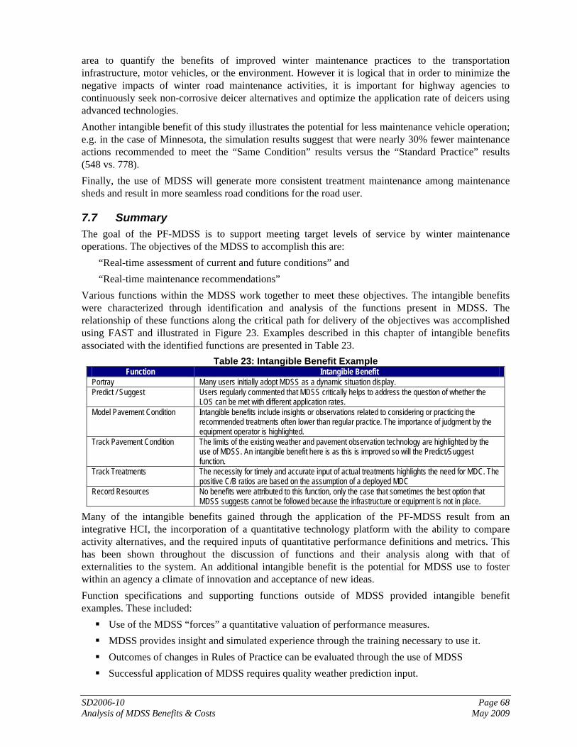
SD2006-10 Page 68 Analysis of MDSS Benefits & Costs May 2009
area to quantify the benefits of improved winter maintenance practices to the transportation infrastructure, motor vehicles, or the environment. However it is logical that in order to minimize the negative impacts of winter road maintenance activities, it is important for highway agencies to continuously seek non-corrosive deicer alternatives and optimize the application rate of deicers using advanced technologies. Another intangible benefit of this study illustrates the potential for less maintenance vehicle operation; e.g. in the case of Minnesota, the simulation results suggest that were nearly 30% fewer maintenance actions recommended to meet the “Same Condition” results versus the “Standard Practice” results (548 vs. 778). Finally, the use of MDSS will generate more consistent treatment maintenance among maintenance sheds and result in more seamless road conditions for the road user.
7.7 Summary The goal of the PF-MDSS is to support meeting target levels of service by winter maintenance operations. The objectives of the MDSS to accomplish this are:
“Real-time assessment of current and future conditions” and “Real-time maintenance recommendations”
Various functions within the MDSS work together to meet these objectives. The intangible benefits were characterized through identification and analysis of the functions present in MDSS. The relationship of these functions along the critical path for delivery of the objectives was accomplished using FAST and illustrated in Figure 23. Examples described in this chapter of intangible benefits associated with the identified functions are presented in Table 23.
Table 23: Intangible Benefit Example Function Intangible Benefit
Portray Many users initially adopt MDSS as a dynamic situation display. Predict / Suggest Users regularly commented that MDSS critically helps to address the question of whether the
LOS can be met with different application rates. Model Pavement Condition Intangible benefits include insights or observations related to considering or practicing the
recommended treatments often lower than regular practice. The importance of judgment by the equipment operator is highlighted.
Track Pavement Condition The limits of the existing weather and pavement observation technology are highlighted by the use of MDSS. An intangible benefit here is as this is improved so will the Predict/Suggest function.
Track Treatments The necessity for timely and accurate input of actual treatments highlights the need for MDC. The positive C/B ratios are based on the assumption of a deployed MDC
Record Resources No benefits were attributed to this function, only the case that sometimes the best option that MDSS suggests cannot be followed because the infrastructure or equipment is not in place.
Many of the intangible benefits gained through the application of the PF-MDSS result from an integrative HCI, the incorporation of a quantitative technology platform with the ability to compare activity alternatives, and the required inputs of quantitative performance definitions and metrics. This has been shown throughout the discussion of functions and their analysis along with that of externalities to the system. An additional intangible benefit is the potential for MDSS use to foster within an agency a climate of innovation and acceptance of new ideas. Function specifications and supporting functions outside of MDSS provided intangible benefit examples. These included:
Use of the MDSS “forces” a quantitative valuation of performance measures. MDSS provides insight and simulated experience through the training necessary to use it. Outcomes of changes in Rules of Practice can be evaluated through the use of MDSS Successful application of MDSS requires quality weather prediction input.
SD2006-10 Page 69 Analysis of MDSS Benefits & Costs May 2009
Quality recommendations from MDSS are reliant upon properly sited, appropriately maintained, and reliable ESS.
Intangible benefits can also result from externalities (uncompensated direct impact to non-MDSS users). Several were identified:
Theoretically, reduced snow and ice control chemicals will result in slower deterioration of reinforced concrete structures.
Less tonnage of chemicals used logically lead to reduced aesthetic impacts, infrastructure and vehicle corrosion, but not reduced costs per ton.
Use of MDSS suggests a reduction in number of maintenance vehicle round trips to meet the historical level of service.
Several observations were made by the project team during the analysis of intangible benefits. The project team suggests that this cost benefit analysis, specifically the simulation methodology used, has resulted in intangible benefits. Other observations include:
The simulation methodology used in the determination of the tangible costs and benefits is a valuable strategic tool resulting from PF-MDSS technology that allows for the investigation of fundamental changes to performance measures, rules of practice, and policy.
Though the Weather Prediction function is outside of the MDSS, cost and quality of such is vital to any bottom-line assessment of cost, benefit, and value and choice of MDSS use.
The PF-MDSS provides value and intangible benefit if used solely as integration / predict / suggest / portray function combining weather prediction, automated weather observations, and rules of practice.
A potential improvement of the PF-MDSS can be realized through the inclusion of additional operational rules of practice. These may take the form of geographical and inventory logic to resources e.g. “this is an out and back route with two trucks available, one with ten cubic yards, the second eight cubic yards” or “this is a one way route with X amount of material at the end.”
A significant potential improvement to the Predict / Suggest / Portray functions of the MDSS in the form of uncertainty communication of the prediction being presented in a front-line context in addition to similar interpretation results occurring by changing parameters in a ‘what if scenario’.
There is high potential for strong intangible benefit of MDSS if results of the Model Pavement Conditions as presented in Predict and Suggest can be used in decision support of the adjacent maintenance segments for a given station without the deployment costs of defining the parameters for those segments.

SD2006-10 Page 70 Analysis of MDSS Benefits & Costs May 2009
8. FINDINGS AND CONCLUSIONS This previous chapters presented a benefit-cost analysis of deploying MDSS for winter maintenance. A methodology that consisted of a baseline data module and a simulation module was developed and applied to three pooled fund states (New Hampshire, Minnesota, and Colorado) to analyze tangible benefits. Tangible costs were calculated based on winter maintenance information requested from the case study state DOTs. In addition, a FAST method was used to assist in identifying the intangible benefits and intangible costs of MDSS. This chapter summarizes the main findings and conclusions of this research study, which are summarized as follows:
1. The exhaustive literature review on weather effects on the roadway system found that, despite of numerous studies in this area, there has been wide variance in the quantitative effects of adverse weather. Thus, a synthesis of these effects was presented in this study to help quantify the safety and mobility benefits of deploying MDSS.
2. The stakeholder interviews revealed that the interviewees generally had a positive view of the PF-MDSS. They generally perceived it as a valuable tool/component for winter maintenance. They believed that MDSS has the potential to help them improve winter maintenance operations, reduced material use, improved scheduling/assignment of personnel, and improved decision making. Respondents from several states also mentioned its potential as an effective training tool. Finally, the level of trust and use of MDSS were anticipated to increase as technical difficulties (communications/computers) were resolved and, as a result, lead to more technological advances in winter maintenance.
3. Through literature review and stakeholder interviews, the research team developed a taxonomy of MDSS benefits and costs. It was perceived that there were three types of benefits and costs associated with the use of MDSS: agency, user (motorists), and society. By using MDSS as a simulator, three benefits including reduced material use (agency benefit) and improved safety and mobility (motorist benefits) were able to be quantified. The methodology for benefit-cost analysis was developed to analyze these tangible benefits and costs.
4. By comparing the actual material use and the simulated use, it was found that they had similar results. This indirectly validates the simulation-based methodology. The analysis method provided the capability of comparing different implementation scenarios and looking at different maintenance results by using rules of practice and MDSS recommendations.
5. Three case studies collectively showed that the benefits of using MDSS outweighed associated costs. The benefit-cost analysis results are presented in Table 24. The benefit-cost ratios did not indicate which MDSS scenario was (always) better. However, it is most likely that an agency implementing MDSS would fall somewhere between the Same Resources scenario and the Same Condition scenario, seeking to achieve both a level of service improvement and a reduction in winter maintenance costs. The case studies also showed that there is a trade-off between agency benefits and user benefits. Increased use of material will achieve more motorist benefits, while increasing agency costs, and vise versa.

SD2006-10 Page 71 Analysis of MDSS Benefits & Costs May 2009
Table 24: Summary of Benefits and Costs Case State Scenario Benefits Percent of User
Savings (%) Percent of Agency
Savings (%) Costs B-C Ratio
Same Condition $2,367,409 50 50 7.11 New Hampshire Same Resources $2,884,904 99 1 $332,879 8.67
Same Condition $3,179,828 51 49 6.40 Minnesota Same Resources $1,369,035 187 -87 $496,952 2.75 Same Condition $3,367,810 49 51 2.25 Colorado Same Resources $1,985,069 90 10 $1,497,985 1.33
6. The intangible benefits were characterized through identification and analysis of the functions present in MDSS. Examples of intangible benefits include: Use of the MDSS “forces” a quantitative valuation of performance measures. MDSS provides insight and simulated experience through the training necessary to use it. Outcomes of changes in Rules of Practice can be evaluated through the use of MDSS Successful application of MDSS requires quality weather prediction input. Quality recommendations from MDSS are reliant upon properly sited, appropriately maintained,
and reliable ESS. 7. Intangible benefits can also result from externalities (uncompensated direct impact to non-MDSS
users), including the following: Less tonnage of chemicals used logically lead to reduced impacts on transportation
infrastructure, motor vehicles, and the environment. Use of MDSS suggests a reduction in number of maintenance vehicle round trips to meet the
historical level of service. Use of MDSS will generate more consistent treatment maintenance among maintenance sheds
and result in more seamless road conditions for the road user.

SD2006-10 Page 72 Analysis of MDSS Benefits & Costs May 2009
9. STAKEHOLDER OUTREACH PLAN The objective of the stakeholder outreach plan is the efficient distribution of key results and recommendations of the analysis. The core findings are contained in the Final Report and Tech Memo 2. The salient components of this need are to be accessible both to the participating pooled fund states as well as elected officials and state DOT decision makers. The outreach plan contains three communication components:
with participant agency personnel with Pooled fund study members with the larger transportation community
In addition to the three reports created by the study (Tech Memos 1 &2, Final Report), three materials support the outreach plan. The first is one-sheet, two-sided brochure describing the study and containing highlights of the methodology and findings. The second is a webpage summarizing the methodology, results, and conclusions in slightly greater depth. The page also provides links to portable document format (.pdf) copies of the three study reports. The third is the publication of a TRB paper focusing on one of the case study states in the analysis. The transportation community will be apprised of the webpage through various winter maintenance and road weather list-servers. It is important to revisit the State DOT personnel who contributed to the study. The opportunity to provide a web-based meeting with these personnel will be considered and discussed with the pooled fund study participants.

SD2006-10 Page 73 Analysis of MDSS Benefits & Costs May 2009
10. IMPLEMENTATION RECOMMENDATIONS The quality of MDSS recommendations relies on the accuracy of input information, which mainly includes recent and current road and weather information. In light of this, it is of importance for transportation agencies to use accurate weather forecast services. In addition, the use of MDC and other technologies can improve the efficiency of two-way communications between MDSS and truck operators and further increase operators’ levels of acceptance of and trust in the MDSS. It is encouraged to use such devices to help fulfill functions of MDSS and achieve maximum benefits. The deployment of MDC and other technologies, however, will increase agency costs. The results of this research study are useful to the MDSS PFS states as well as other government agencies. Due to the complexity of the methodology and the need for numerous good-quality data related to climatic and traffic conditions as well as winter maintenance activities, it would take significant amount of time and efforts for another state DOT or transportation agency other than the three case study states to conduct a similar cost-benefit analysis of MDSS. Hence, a simplified approach is provided as follows for any transportation agency that desires to derive an approximate yet defensible benefit-cost ratio.
MDSS costs can be calculated through cost breakdown as shown in tables 13, 17, and 20. Important information for calculating MDSS costs includes the number of garages (sheds), the number of MDCs, and administrative cost (in terms of an assumed percentage of direct costs).
The calculation of benefits is complex if following the methodology provided in this study. However, through the investigation into the benefits of the “Same Condition” scenario and material costs, it is found that the ratios of benefits over materials costs are 0.31, 0.36, and 0.30 for the three case studies. Hence, to be conservative, a state DOT may simply calculate the benefits by using 0.30 of total material costs per winter season. It is worth noting that under the “Same Condition” scenario, approximate half of the benefits are agency benefits and the other half are motorist benefits.
Table 25: Use of Case Study Results Benefits ($ 000s)
Case State Climate Material Costs
($ 000s)*
MDSS Costs
($ 000s) Same
Resources Same
Condition Ratio*
New Hampshire
Transition (Freezing Rain) State 7,499 332 2,885 2,367 0.31
Minnesota Northern Plains State 8,817 497 1,369 3,179 0.36 Colorado Mountain/West State 11,099 1,498 1,985 3,368 0.30
*: The ratio is calculated by the benefits in the “Same Condition” scenario over material costs.
This research study provided methods for the calculation of agencies benefits and motorist benefits (reduced travel time and improved traffic safety). Interested organizations (e.g., universities and private enterprise) can use the methods for their own purposes, i.e., benefit-cost analysis for other technologies.

SD2006-10 Page 74 Analysis of MDSS Benefits & Costs May 2009
11. REFERENCES 1. “Maintenance Decision Support System (MDSS),” Priority, Market-Ready Technologies and
Innovations, Publication FHWA-HRT-06-039, Federal Highway Administration, Washington [DC]: January 2006. Available at http://www.fhwa.dot.gov/crt/marketready/mdss.pdf on August 1, 2006.
2. Pisano, P., A. Stern and D. Huft, “Deployment of the Maintenance Decision Support System for Winter Operations,” presented at 11th AASHTO-TRB Maintenance Management Conference, Charleston [SC]: July 18, 2006.
3. Huft, David, “Maintenance Decision Support System Pooled Fund Study TPF-5(054),” presentation given at MDSS Stakeholders Meeting, Boulder, Colorado, October 20-21, 2005.
4. Hart, R. and L.F. Osborne, Development of a Maintenance Decisions Support System—Phase 1, Report No. SD2002-18-I, Prepared for the South Dakota Department of Transportation, Meridian Environmental Technology, Grand Forks [ND]: December 16, 2003.
5. Hart, R., L. Osborne, and J. Mewes, Development of a Maintenance Decision Support System Interim Report: Draft Phase IV Interim Report, Report No. SD2002-18-I-4, South Dakota Department of Transportation, January 2008.
6. Mitretek Systems, Surface Transportation Weather Decision Support Requirements Version 1.0, Prepared for Federal Highway Administration Office of Transportation Operations, January 24, 2000.
7. Mewes, J, R Hart, L. Osborne and B. Podoll, The Pooled Fund Study Maintenance Decision Support System: A Functional Overview. American Meteorological Society Preprint, the 21st International Conference on Interactive Information Processing Systems (IIPS), San Diego, CA, 2005, Paper 6.6.
8. Federal Highway Administration, Economic Analysis Primer, Publication No. FHWA IF-03-032, Office of Asset Management, Federal Highway Administration, U.S. Department of Transportation, Washington [DC]: August 2003.
9. C. Lee and B. Ran, “A Pilot Study to Measure the Potential of Using Speed Recovery Duration as a Winter Maintenance Performance Measures,” Presented at the 2004 Transportation Research Board Annual Meeting.
10. J. McBride, W. Kennedy, J. Thuet, M. Belangie, R. Stewart, C. Sy and F. McConkie, Economic Impact of Highway Snow and Ice Control, Report No. FHWA-RD-77-95, Federal Highway Administration, U.S. Department of Transportation, Washington [DC]: 1977.
11. J. Thornes, “The Cost-Benefit of Winter Road Maintenance in the United Kingdom,” Proceedings of the Eighth International. Road Weather Conference, University of Birmingham [UK], Birmingham [UK], 1996, pp. 1-10.
12. J. Thornes, “A Benefit-cost Review of the Use of Safecote Additives to Rock Salt for the Winter Maintenance of Roads in the UK,” Jetmet Services, Worcestershire [UK], November 2003.
13. T. Maze, M. Crum and G. Burchett, An Investigation of User Costs and Benefits of Winter Road Closures, Midwest Transportation Consortium, Iowa State University, June 2005.
14. K. Knapp, D. Kroeger and K. Giese, “Mobility and Safety Impacts of Winter Storm Events in a Freeway Environment: Final Report,” Center for Transportation Research and Education, Iowa State University, February 2000.

SD2006-10 Page 75 Analysis of MDSS Benefits & Costs May 2009
15. T. Maze, M. Agarwal and G. Burchett, Whether Weather Matters to Traffic Demand, Traffic Safety, and Traffic Flow, Prepared for the Aurora Program by the Center for Transportation Research and Education, Iowa State University, Ames [IA]: August 2005.
16. M. Agarwal, T. Maze and R. Souleyrette, “The Weather and Its Impact on Urban Freeway Traffic Operations,” Presentation at the 2006 Transportation Research Board Annual Meeting.
17. C. Strong, Y. Shvetsov and J. Sharp, Development of a Roadway Weather Severity Index: Final Technical Report, Western Transportation Institute, Montana State University, August 2005.
18. J. Mewes, “Transition Plans to Broader Deployment,” Presented at MDSS Pooled Fund Meeting, Sioux Falls [SD]: February 21, 2007.
19. U.S. Department of Transportation, “Departmental Guidance for the Valuation of Travel Time in Economic Analysis,” Office of the Secretary of Transportation, U.S. Department of Transportation, 1997. Accessed at: http://ostpxweb.dot.gov/policy/Data/VOT97guid.pdf on March 19, 2007.
20. U.S. Census Bureau, “The 2007 Statistical Abstract: The National Data Book,” Accessed at http://www.census.gov/compendia/statab/ on March 19, 2007.
21. Transport Canada, Guide to Benefit-Cost Analysis in Transport Canada, Publication No TP11875E, Transport Canada, September 1994.
22. MacQueen, J.B. Some Methods for classification and Analysis of Multivariate Observations, Proceedings of 5-th Berkeley Symposium on Mathematical Statistics and Probability, Berkeley, University of California Press, 1:281-297, 1967.
23. Federal Highway Administration, Motor Vehicle Accident Costs, Report No. T 7570.2, October 1994.
24. New Hampshire Department of Transportation, NHDOT – Business Center, Accessed at http://www.nh.gov/dot/transportationplanning/traffic/index.htm#atr on January 4, 2008.
25. Keen, P. G. W. Value analysis: justifying decision support systems. MIS Quarterly 5(No 1 (March 1981)), pp. 1-15.
26. Kaufman, J. J., and Woodhead, R. Stimulating innovation in products and services with function analysis and mapping, John Wiley & Sons, Inc, Hoboken, 2006.
27. Meridian Environmental Technology. Development of a maintenance decision support system interim report SD2002-18 Draft Phase IV Interim Report. Grand Forks, 2008.
28. Dörner, D. The Logic of Failure: Why things go wrong and what we can do to make them right, Metropolitan Books, New York, 1996.
29. Shi, X., Fay, L., Yang, Z., Nguyen, T.A., and Liu, Y. Corrosion of Deicers to Metals in Transportation Infrastructure: Introduction and Recent Developments. Corrosion Reviews 2009, 27(1-2), 23-52.
30. Shi, X., Akin, M., Pan. T., Fay, L., Liu, Y., and Yang, Z. Deicer Impacts on Pavement Materials: Introduction and Recent Developments. The Open Civil Engineering Journal 2009, 3, 16-27.
31. Staples, J.M., Gamradt, L., Stein, O., and Shi, X. Recommendations for Winter Traction Materials Management on Roadways Adjacent to Bodies of Water. Montana Department of Transportation. Helena, MT, December 2004. FHWA/MT-04-008/8117-19. Available at http://www.mdt.mt.gov/research/docs/research_proj/traction/final_report.pdf on May 1, 2009.
32. Shi, X., Fay, L., Gallaway, C., Volkening, K., Peterson, M.M., Pan, T., Creighton, A., Lawlor, C., Mumma, S., Liu, Y., and Nguyen, T.A. Evaluation of Alternate Anti-icing and Deicing

SD2006-10 Page 76 Analysis of MDSS Benefits & Costs May 2009
Compounds Using Sodium Chloride and Magnesium Chloride as Baseline Deicers. Final Report for the Colorado Department of Transportation. Denver, CO. Report No. CDOT-2009-01. January 2009. Available at http://www.dot.state.co.us/Publications/PDFFiles/antiicing.pdf on May 1, 2009.
33. Shi, X. The Use of Road Salts for Highway Winter Maintenance: An Asset Management Perspective. 2005 ITE District 6 Annual Meeting. Kalispell, Montana. July 10-13, 2005.
34. Vitaliano, D. Economic Assessment of the Social Costs of Highway Salting and the Efficiency of Substituting a New Deicing Material. Journal of Policy Analysis and Management 11(3), 1992, pp.397-418.

SD2006-10 Page 77 Analysis of MDSS Benefits & Costs May 2009
Appendix A: Questionnaire for State DOT Stakeholders
A. Establish Frame of Reference
1. `What is your role/position in winter maintenance practice in your region/state? (For example, do you run routes? Do you manage vehicle operators at a shed? Do you track maintenance operations from a regional level? Do you establish rules of practice and guidelines for winter maintenance procedures?)
2. What are your winter maintenance objectives?
3. What are the major winter maintenance challenges in your state?
4. How concerned is your organization with customer satisfaction?
5. To what extent does your organization provide information to the public on the level of winter road maintenance being performed; per season, per storm event; per route?
6. Do you feel your organization’s level of winter road maintenance exceeds what is necessary to maintain road mobility?
7. Do you feel your organization’s level of winter road maintenance exceeds what is necessary to maintain road safety?
8. What precautions are taken to increase public and worker safety during storm events?
9. When the level of winter road maintenance is prescribed are the long term impacts to infrastructure, environment and vehicles considered?
10. When considering mobility versus safety, is the economic impact from the prescribed level of service considered? Is the economic impact from the loss of mobility considered? Is the economic impact from decreased driver safety considered?
11. To what extent is the level of winter road maintenance tailored to maintain road mobility for: the public, freight/commercial, workers?
12. To what level of detail can you determine the costs associated with winter road maintenance; Plow/Truck, Fleet, Shed, Chemical use, or are all of these grouped? Do you use a storm severity index when reporting on storm events?
B. Base Case
Maintenance Decision Process
13. At what level in your organization is the decision made on the type of winter road maintenance that is performed?
14. At what level in your organization is the decision made on the application rate of the deicer?
15. How are these decisions communicated to the field technicians?
16. What method of communication do you use between your maintenance shed office and your deployed vehicles?

SD2006-10 Page 78 Analysis of MDSS Benefits & Costs May 2009
17. If maintenance managers make recommendations on maintenance treatments (e.g. chemical/material and application rate), what information sources do they have available (e.g. National Weather Service, RWIS, camera images of roads)?
18. If conditions change while field technicians are deployed is there leeway for field technicians to alter the original level of maintenance that was prescribed?
19. If vehicle operators are permitted to make decisions on application rate or maintenance treatments while in the field, what information sources do they have available (e.g. temperature sensors)?
20. How are vehicle operators trained for making winter maintenance decisions?
Type of Treatment Practices
21. Does your organization use anti-icing techniques in winter road maintenance?
22. For what percentage of storms would you guess that anti-icing techniques are applied? And is it safe to assume that in the remaining percentage of storms de-icing techniques are used?
23. Do you trust anti-icing as a method of winter road maintenance?
24. To what extent are impacts to the infrastructure or the environment considered in the costs of applied anti-icers/deicers?
Importance of Weather Information
25. How does your organization use weather information with respect to making winter road maintenance treatment decisions?
26. How many storm events per season do you fail to respond to in a timely fashion because of errant (wrong) weather forecasts?
27. What are the impacts to your transportation agency if a storm is inaccurately forecasted (e.g. hurts public relations, takes long time to recover roads)?
28. Can you put an estimated economic value on this?
29. How many times per season do you take proactive action for winter storms which fail to materialize? What are the impacts of this; economic, public relations, etc.?
C. MDSS
Frame of Reference
30. What is your level of experience with MDSS? (For example, received training on it, use it occasionally, use it regularly)
31. How would/does MDSS support your winter maintenance objectives?
32. What expectation did you have with implementing MDSS? Has MDSS met these expectations?
33. At what scale has MDSS been implemented (e.g. how many sections of road; how many sheds; which level of road priority)?
34. How often do you use the MDSS program; seasonally or per storm event?

SD2006-10 Page 79 Analysis of MDSS Benefits & Costs May 2009
Maintenance Decision Process
35. Do you think MDSS would change where in your organization winter maintenance treatment decisions are made?
36. How valuable will MDSS be if it provides information only to a server in a maintenance office?
37. Would it be more valuable to have MDSS in vehicle (plow/truck) for easy access by vehicle operators?
Types of Treatment Practices
38. How do you think implementing MDSS would change the current state of practice?
39. Would you want your state’s rules of practices to be coded into MDSS? Why or why not?
40. Have you noticed that implementing MDSS has changed any rules of practice?
41. Did your organization use anti-icing techniques prior to acquiring MDSS?
42. To what extent are the MDSS prescribed treatments limited by resource constraints?
Level of Trust
43. Do you trust the prescribed treatment suggested by MDSS?
44. How often do you implement the prescribed treatment suggested by MDSS?
45. Have you ever considered the MDSS prescribed treatment but not followed the suggestion? Why?
46. Do you perceive the recommendations from MDSS more as “guidance”, or as “directive”?
47. Do you foresee a time when a vehicle operator, a shed, a region or your entire state would use the MDSS treatment recommendations as directive? What would need to happen for that to occur?
48. If MDSS suggested you use anti-icing to treat a route you normally do not treat with anti-icing, would you consider this suggestion? Would you then implement this suggestion?
49. If MDSS suggested a higher application rate for anti-icing/deicing than what has been historically used, would you consider this suggestion? Would you then implement this suggestion? (For example you normally apply 20 g/l-m of anti-icer on a section of road and MDSS suggests you apply 40 g/l-m)
50. If MDSS suggested a lower application rate for anti-icer/deicer than what has been historically used, would you consider this suggestion? Would you then implement this suggestion? (For example you normally apply 40 g/l-m of anti-icer on a section of road and MDSS suggests you apply 20 g/l-m)
51. When using MDSS, does your organization ever use “ground truthing” to confirm that the MDSS conditions are the same as the actual road conditions?
52. Do you feel your recommendations/input is heard by MDSS vendor? Do you feel your recommendations/input to MDSS vendor has improved the system?

SD2006-10 Page 80 Analysis of MDSS Benefits & Costs May 2009
Informal Performance Assessment
53. With the use of MDSS, have you noticed an increase in road mobility?
54. Does your organization feel MDSS has saved your organization money? Please provide examples.
55. Do you think that MDSS has helped to improve road safety? Please provide examples.
56. Have you noticed any trends in how MDSS performs with respect to weather severity, frequency or forecast ability?
57. Does your organization use post storm debriefing to discuss how effectively the level of winter road maintenance was implemented? Is this feature critical to the value of MDSS to your agency?
58. How aware are you of your driver’s direct experience with the MDSS program? (i.e. Positive and negative feed back, do you take into consideration their experiences when evaluating MDSS?)
59. Can you list any other tangible and intangible benefits that might be gained from implementing MDSS?

SD2006-10 Page 81 Analysis of MDSS Benefits & Costs May 2009
Appendix B: Questionnaire for Meridian Stakeholders A. Frame of Reference
1. What roles have you had in the use, design, implementation of the pooled fund version MDSS system?
2. Have you been involved with the MDSS system from the beginning?
3. Have you had any direct contact with MDSS users?
B. Evolution of MDSS
4. The pooled fund MDSS has been defined to include five functions; for each of these functions, describe how the MDSS has evolved, and to what extent the MDSS can be improved.
a. assess current road and weather conditions using observations and reasonable inferences based upon observations;
b. provide time- and location-specific weather forecasts along transportation routes;
c. predict how road conditions would change due to the forecast weather and the application of several candidate road maintenance treatments;
d. notify state agencies of approaching conditions and suggest optimal maintenance treatments that can be achieved with resources available to the transportation agencies; and
e. evaluate the reliability of predictions and the effectiveness of applied maintenance treatments for specific road and weather conditions so decision support can be improved.
5. How do you think implementing MDSS would change the current state of practice?
6. Do you feel Meridian is open to revising MDSS because of user suggestions?
7. Have there been user suggestions that Meridian has been unable to address or find solutions to?
8. In what states has Meridian done “ground truthing” to test road condition forecasts versus actual road conditions?
9. Do you feel users of MDSS sending an error message that the weather/prescribed treatment is inaccurate will help modify the system/algorithm?
10. To what level of detail do you think/know MDSS can be used?
11. For a defined road segment is there a maximum number of MDSS routes that it can be assigned?
12. If an agency with MDSS decided to create another route on a road section that previously has not had one, would it be expected that their forecast provider would need to refine their models for the new route?
13. Is there a way for the MDSS system to adjust the recommendations of deicer use up/down a slope with the changing volume of snow, ice, and rain?

SD2006-10 Page 82 Analysis of MDSS Benefits & Costs May 2009
14. Some users have expressed concern about manually updating the system regarding maintenance vehicle activity during dangerous inclement weather. To prevent this, AVL technology could monitor road conditions and relay data directly so that the plow driver does not need to. Do you see this technology being implemented?
15. For DOT sheds using MDSS without road pavement temperature sensors, air temperature sensors and ground speed measurements, do you think the MDSS system will perform equally as well as a shed with these technologies?
16. Do you see MDSS changing existing winter maintenance practices?
17. Have you ever communicated with previous vendors (e.g. the Feds) while working on the system?
18. Have you received any comments on dead spots for radio communication, radar, uploading data to the system?
C. MDSS Vehicle Interface
19. Can you briefly talk about the evolution of the vehicle interface?
20. What are the capabilities of the vehicle interface?
21. What functionality of the MDSS system might be missing if the vehicle interface is not used?
22. Have you received any user comments on vehicle-based or server-based issues? Interface issues?
D. MDSS Assessment
23. How do you see MDSS being used?
24. Do you see MDSS as being superior to existing winter maintenance practices? And if so can list specifically how MDSS does this?
25. What benefits do you associate with using MDSS?
26. Have you received any comments from agencies that reported improvements over time (for example, quicker restoration of bare pavement) after implementing MDSS?
27. Are you aware of any instances where agencies followed MDSS recommendations instead of their current practice and found the results to be worse (for example, the need to perform additional maintenance routes)? If so, what seemed to be contributing factors to these cases?
28. Under what circumstances would an agency not benefit from MDSS?
29. Describe your level of trust/confidence for the different components of the MDSS system?
30. If a user is having a lack-of-trust issue in MDSS, what would you recommend?
31. Do you perceive the recommendations from MDSS more as “guidance”, or as “directive”?

SD2006-10 Page 83 Analysis of MDSS Benefits & Costs May 2009
E. MDSS Costs and Procurement
32. How much does MDSS supplied by Meridian cost?
33. What would like to see MDSS compared too to best illustrate its value?
34. If a state is currently in the start up phase of MDSS (a pooled fund member/stakeholder) and two years from now wants to add new routes, sheds, regions or want to extend existing routes in the MDSS system, what sort of costs would there be?
35. If a non-pool fund member/stakeholder state wants to use MDSS what would be the start up cost?
36. For pooled fund member states, are there costs for upgrades to the systems, and for server and user support?
37. Are you familiar with the MDSS Functional Specification Template and Procurement Guidance, prepared by the National Center for Atmospheric Research (NCAR)?
a. If so, are there any areas of the specification that the pooled fund MDSS does not comply with?
b. If there are areas where the pooled fund MDSS is non-compliant with the specification, does Meridian plan to address those? If so, how? If not, why not?
F. MDSS in the Future
38. Where do you see MDSS in the future?
a. What can users do to aid in accomplishing this?
39. What form of communication system would ideally suit MDSS?
40. Once the final version of MDSS is in place, do you think the program could be modified as easily/frequently from user suggestions?
41. What does it take to realize the full benefits of MDSS?

SD2006-10 Page 84 Analysis of MDSS Benefits & Costs May 2009
Appendix C: Use of MDSS as a Simulator Due to serious limitations in the data available to support analysis, the approach taken in the Pooled Fund Study (PFS) MDSS cost/benefit study has been to use the available data wherever possible and then to fill in the missing information using a simulation approach. In this simulation approach, historical weather information is provided to the PFS MDSS modeling system, which then simulates both the road conditions and maintenance activities that should have resulted in response to those weather conditions. The following sections discuss the simulation approach in greater detail.12
Simulation System Components
Weather Information The data that are being used in this study come from four different sources: National Weather Service (NWS) hourly Meteorological Aviation Reports (METAR) observations from the National Climatic Data Center (NCDC), hourly METAR observations from the Meteorological Assimilation Data Ingest System (MADIS), the North American Regional Reanalysis (NARR) from the National Centers for Environmental Prediction (NCEP), and blowing snow information generated from a modified version of the Functional Prototype (FP) Maintenance Decision Support System (MDSS) blowing snow module. The NWS hourly METAR observations from NCDC cover dates spanning from 1996-2006, while the MADIS hourly observations cover from 2006-present. The reason for the transition is due to the fact that the NCDC observation database that was originally used lagged real-time by 6 months to a year, thereby prohibiting simulation of recent history. The MADIS observations were acquired to fill in the more recent periods of the dataset. The METAR observations are used to provide temperature, relative humidity, wind speed, present weather, and other pertinent information to the PFS MDSS modeling system. Precipitation type and rate information is derived using algorithms that take into account the present weather, visibility and wind speed information. Holes in the observational database for a given station of less than 6 hours were time interpolated. Holes exceeding 6 hours in length were filled by using data from another nearby station. The NARR data was acquired to provide the downwelling long- and short-wave radiation required by the modeling system. Although estimation of the radiation budgets based on METAR observations (including cloud cover) would have been possible, the altitude limitation of METAR cloud cover observations would likely have had serious impacts on the reliability of those estimates in the presence of high clouds. The last type of weather information required by the PFS MDSS modeling system is an estimate of the blowing/drifting snow mass flux across roadways. Since observations of this mass flux are unavailable, and since drifting snow often occurs without being observed in the METAR data, this blowing snow mass flux needed to be estimated from the information that was available. The blowing snow algorithm developed for the MDSS Functional Prototype (FP) by the National Center for Atmospheric Research (NCAR) was chosen to serve this purpose due to its suitability to blowing snow risk assessment with a history of METAR observations. This module uses surface weather observations to generate an index indicating the severity of the blowing snow risk. The algorithm looks at temperature, precipitation, wind speed and direction, and snow age using data from the preceding 72 hours. The resulting index was then used to generate horizontal mass flux values that could be inserted into the PFS MDSS modeling system. 12 Readers interested in additional detail should contact John Mewes, Chief Scientist at Meridian Environmental Technologies, at [email protected], who served as the primary source for most of the information provided in this appendix.

SD2006-10 Page 85 Analysis of MDSS Benefits & Costs May 2009
Pavement Model A key premise of the PFS MDSS system and the simulation approach used in this study is that the behavior of the mixture of water, snow, ice and freeze point depressants (the ‘dynamic layer’) atop the roadway is predictable. Predicting its characteristics and evolution require a great deal of sophistication. A key enabling technology for the PFS MDSS was the development of Meridian’s HiCAPS™ pavement condition prediction model, a sophisticated mass and energy balance model that possessed a proven ability to simulate the characteristics of the dynamic layer. The HiCAPS™ model, to allow its use in maintenance decision support, has tapped additional modules developed during the PFS MDSS project. The processes modeled by the PFS MDSS, many through the HiCAPS™ model, are listed in Table 1. Functions for modeling traffic and the effects of freeze-point depressing chemicals placed atop the roadway are newly developed during the Pooled Fund Study, and are held in a library of MDSS-related functions accessible by the HiCAPS™ model. HiCAPS™ forecasts pavement and bridge deck temperatures using what is commonly referred to as the unsteady heat flow equation. It uses sophisticated parameterizations for representing heat and moisture exchanges between the road, the atmosphere, and pavement substrate. A key distinction that sets HiCAPS™ apart from most other pavement models is the coupling between the mass and energy balances in the model. In simple terms, this means that when moisture (as snow, rain, frost, dew, etc.) is deposited onto the road it also transfers energy to or from the road, and that evaporation or sublimation of moisture from the road requires the road to have an adequate amount of energy available to support those processes. This coupling has key implications for the model’s ability to support MDSS in a scientifically sound manner. HiCAPS™ was built to be a robust model, capable of filtering through the occasionally erratic observations that inevitably come from in-pavement sensors. It uses a continuous data assimilation system that adds to HiCAPS™ robustness, as it is able to continue to make reasonably reliable forecasts in the complete absence of RWIS observations (typically less than a 1° F loss of forecast accuracy). Since the goal of MDSS is to provide guidance on entire road networks, this is a key capability. It also serves this study well in that historical RWIS information is generally not available for many of the routes identified as candidates for the study. HiCAPS™ has a sophisticated scheme for handling latent heat fluxes (heat exchanges related to changes in the state of water). This includes modeling of heat exchanges associated with evaporation, sublimation, condensation, deposition (frost formation), and phase changes (e.g., water freezing on the road surface) – naturally or chemically induced. HiCAPS™ also makes actual predictions of the depth of water, ice, frost, compacted snow and snow upon the roadway. This key feature makes HiCAPS™ uniquely adaptable to MDSS modules. For example, HiCAPS™ may project a layer of snow on the pavement based upon a forecast of snow falling at a certain rate. HiCAPS™ can then determine what effect plowing and an application of chemical at a given rate will have on the snow layer using the phase diagram for the applied chemical. Chemical applications change the amounts of snow, ice, and water in the model to reflect the effects of the chemical application on the snow/ice/water layer on the pavement (‘dynamic layer’) that existed before treatment. The result may be a projected “slush” composition based upon the chemical action and any additional precipitation. HiCAPS™ can also adjust the depth of snow left after plowing based upon the plow type and model the effect of traffic based upon the traffic volume and the consistency of the surface material.

SD2006-10 Page 86 Analysis of MDSS Benefits & Costs May 2009
Table 26: Capabilities of the HiCAPS™ Model Used as the Pavement Model of the PFS MDSS Modeling System
Processes Modeled within the PFS MDSS Modeling System Evaporation (mass / energy balanced) Condensation (mass / energy balanced) Sublimation (mass / energy balanced) Frost Formation (mass / energy balanced) Conduction of heat from precipitation Internal heat conduction within pavement Traffic splatter, splash, spray, compaction Snow / ice removal by plow Natural phase changes Chemically induced phase changes Heat exchange between air and pavement Emission of infrared radiation by pavement Absorption of solar and infrared radiation Time-varying pavement reflectance Insulating effects of snow & ice buildup Condition-dependent snow adherence Variable freeze points Water and chemical runoff Chemical dilution Chemical removal by traffic Residual chemical amounts and effects
Other Special Features of the PFS MDSS Modeling System Explicit calculation of liquid, ice, frost, compacted snow and snow depths on the road, allowing for mixed conditions such as slush Support for modeling the effects of freeze-point depressing chemicals Highly configurable pavement and maintenance equipment specifications Coupled mass and energy balance Support for modeling the effects of reported and proposed maintenance actions
MDSS Software Modules The PFS MDSS approach focuses upon simulation of the “dynamic layer” atop the pavement. This is accomplished using a pavement model, HiCAPS™, as per the preceding discussion, coupled with additional modules required for maintenance decision support activities. As an example, a new chemical solution module was developed to support the need for modeling the effects of freeze point depressants on the state of the roadway. The structure of the HiCAPS™™ model was such that the transition to solution modeling required only that a simple fixed freeze point temperature instead be calculated dynamically based upon the chemicals present (all of the associated phase change processes were already handled by the model). In addition to these dynamic freeze points, solution support also required the handling of absorption processes (salts absorbing humidity directly from the air), evaporation reduction due to reduced vapor pressure in solutions, and removal of the chemicals by runoff, traffic, and additional maintenance activities. For simulated plowing operations, the MDSS system estimates the depth of snow and ice remaining behind the plow based upon plow type and the road surface roughness. Immediate material loss during the application process is configurable and dependent upon the form of the material (e.g., dry, prewet, or brine). Also, the depth of materials remaining behind the plow is configurable based upon plow type. Previously applied soluble / insoluble chemicals and grit are removed during plowing at the same fractional rate as the liquid / total moisture mass in the contaminant layer. Due to density considerations, liquid is assumed to preferentially reside near the bottom of the contaminant layer and is therefore generally removed by a plow at a lesser rate than frozen materials within the mixture. Moisture and maintenance materials are also removed by runoff, and by the effects of traffic. Due to the lack of reliable and consistent research data on the cumulative effects of hundreds or thousands of vehicles upon the contaminant layer, the PFS MDSS instead models the effects of traffic on a more tractable vehicle-by-vehicle basis. Based upon average daily auto and truck traffic counts, the MDSS distributes vehicles across the contaminant layer at a rate that varies according to a configurable pattern throughout the day. Each vehicle is assigned a random lane, track and vehicle width, and moisture within the tire tracks is splattered, sprayed, spread, or compacted depending upon the composition of the contaminant layer. Moisture and materials are moved laterally atop the

SD2006-10 Page 87 Analysis of MDSS Benefits & Costs May 2009
roadway, and are also removed from the roadway depending upon the splatter, spray, and spread widths relative to the distance of the tire locations from the edge of the roadway. Maintenance recommendations in the PFS MDSS software can be made by one of two available modules. ‘Standard’ or ‘Best Practices’ for an agency are the predominant means of providing guidance to operators on how to approach maintenance in various situations. This type of guidance may be referred to as an ‘analogue’ approach in that guidance is made by drawing analogies to what has been proven to work in similar situations in the past. One approach to generating recommendations in MDSS is the computerization of these policy documents using what will be referred to herein as the ‘Standard Practice’ recommendation module. Since these documents have been generated based upon proven experiences over time they generally provide a safe, but not necessarily optimal, approach to maintenance. When using this module to make recommendations MDSS is not provided the authority to stray from standard practice in such a situation, and MDSS makes no guarantee that the recommended activity will work. It simply models the impacts of the recommendation and then uses the same module to make additional later recommendations as necessary. Note that while the intended use of this module is to provide recommendations consistent with agency guidelines, it can also be used to simulate the current maintenance practices on any given maintenance route so long as the typical response to various weather and road condition situations can be parameterized into a form usable by the Standard Practice module. This latter capability serves the simulation approach used in this study well in that it can be used to simulate the current maintenance practices being used on any arbitrary route. While field-proven and typically a safe response, Standard Practice recommendations also have drawbacks. One of the most significant is an oversimplification of situations. While road conditions may vary substantially due to traffic, environmental, or other subtle considerations, these types of variances are not typically accommodated by Standard Practice recommendations. Standard Practice guidance also typically leaves the ongoing response to a storm after the completion of the first maintenance action rather vague. Also problematic is the fact that many agencies are exploring the use of new chemicals and there is little or no existing basis upon which the agency can draw to prescribe how these new chemicals should be used. Because of these and other considerations, the PFS MDSS has pursued a parallel approach it refers to as a ‘dynamic’ approach using what will herein be referred to as the ‘Dynamic’ recommendation module. In this approach the characteristics of the dynamic layer, as compared to a configurable goal for its condition, are used as the basis for prescribing maintenance actions. When a condition requiring maintenance is detected, the MDSS can look at crew schedules, available materials, and forthcoming weather and traffic conditions to identify the maintenance approach and timing most likely to yield favorable results. The system accomplishes this by identifying one or more candidate maintenance actions that will adequately maintain the road from a safety / mobility point of view, then selecting the optimal recommendation, which most effectively maintains that condition based upon cost, environmental impact, or other considerations. The recommendations provided by this Dynamic module serve as the approach to maintenance that would have been recommended by MDSS (in contrast to the current maintenance approach, which is simulated by the Standard Practice module).
Simulation Approach The first step in the simulation process is to identify the maintenance route for the simulation and acquire historical records from the appropriate agency regarding maintenance resources expended on that route. In some instances this information is available on a daily basis, in others it may be weekly, monthly or even seasonal in nature. The minimum information required includes the type and amount of material(s) applied over discrete periods of time. Additional information regarding the number and/or timing of maintenance runs is also useful, as is any corresponding road condition information.
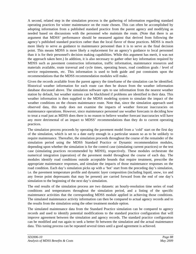
SD2006-10 Page 88 Analysis of MDSS Benefits & Costs May 2009
A second, related step in the simulation process is the gathering of information regarding standard operating practices for winter maintenance on the route chosen. This can often be accomplished by adopting information from a published standard practice from the parent agency and modifying as needed based on discussions with the personnel who maintain the route. (Note that there is an argument that MDSS’ performance should be measured against that derived from following the agency’s published standard practices rather than the local flavor of those practices. MDSS is much more likely to serve as guidance to maintenance personnel than it is to serve as the final decision point. This means MDSS is more likely a replacement for an agency’s guidance to local personnel than it is for their personnel's decision making capabilities. While this argument has merit, it was not the approach taken here.) In addition, it is also necessary to gather other key information required by MDSS such as pavement construction information, traffic information, maintenance resources and materials available, route traversal and cycle times, operating hours, road condition goals / level of service requirements, etc. This information is used to both guide and put constraints upon the recommendations that the MDSS recommendation modules will make. Given the records available from the parent agency the timeframe of the simulation can be identified. Historical weather information for each route can then be drawn from the weather information database discussed above. The simulation software opts to use information from the nearest weather station by default, but weather stations can be blacklisted if problems are identified in their data. This weather information is then supplied to the MDSS modeling system to simulate the impact of the weather conditions on the chosen maintenance route. Note that, since the simulation approach used observed data, this study does not examine the impacts of weather forecast inaccuracies on maintenance operations. However, since maintenance personnel use weather forecasts in deciding how to treat a road just as MDSS does there is no reason to believe weather forecast inaccuracies will have any more detrimental of an impact to MDSS’ recommendations than they do to current operating practices. The simulation process proceeds by operating the pavement model from a ‘cold’ start on the first day of the simulation, which is set to a date early enough in a particular season so as to be unlikely to require maintenance. Thereafter, the simulation proceeds throughout the course of the remainder of the simulation period using the MDSS Standard Practice or Dynamic recommendation modules, depending upon whether the simulation is for the control case (simulating current practices) or the test case (simulating practices recommended by MDSS), respectively. These modules orchestrate the numerical integration (operation) of the pavement model throughout the course of each day. The modules identify road conditions outside acceptable bounds that require treatment, prescribe the appropriate maintenance responses, and simulate the impacts of those maintenance responses on the road condition. Each day’s simulation picks up with a ‘hot’ start from the preceding day’s simulation, i.e. the pavement temperature profile and dynamic layer composition (including liquid, snow, ice and any freeze point depressants that may be present) are carried forward from the end of one day’s simulation to the beginning of the next day’s simulation. The end results of the simulation process are two datasets: an hourly-resolution time series of road conditions and temperatures throughout the simulation period, and a listing of the specific maintenance activities that the corresponding MDSS module applied in achieving those conditions. The simulated maintenance activity information can then be compared to actual agency records and to the results from the simulation using the other treatment module option. The simulated maintenance data from the Standard Practice simulation can be compared to agency records and used to identify potential modifications to the standard practice configuration that will improve agreement between the simulation and agency records. The standard practice configuration can be modified and run again to seek a better fit between the simulation and the actual maintenance data. This tuning process can be repeated several times until a good agreement is achieved.
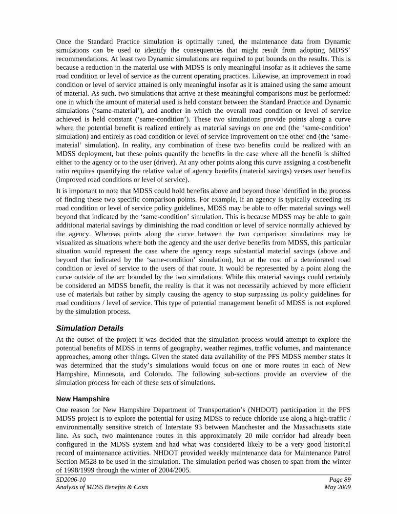
SD2006-10 Page 89 Analysis of MDSS Benefits & Costs May 2009
Once the Standard Practice simulation is optimally tuned, the maintenance data from Dynamic simulations can be used to identify the consequences that might result from adopting MDSS’ recommendations. At least two Dynamic simulations are required to put bounds on the results. This is because a reduction in the material use with MDSS is only meaningful insofar as it achieves the same road condition or level of service as the current operating practices. Likewise, an improvement in road condition or level of service attained is only meaningful insofar as it is attained using the same amount of material. As such, two simulations that arrive at these meaningful comparisons must be performed: one in which the amount of material used is held constant between the Standard Practice and Dynamic simulations (‘same-material’), and another in which the overall road condition or level of service achieved is held constant (‘same-condition’). These two simulations provide points along a curve where the potential benefit is realized entirely as material savings on one end (the ‘same-condition’ simulation) and entirely as road condition or level of service improvement on the other end (the ‘same-material’ simulation). In reality, any combination of these two benefits could be realized with an MDSS deployment, but these points quantify the benefits in the case where all the benefit is shifted either to the agency or to the user (driver). At any other points along this curve assigning a cost/benefit ratio requires quantifying the relative value of agency benefits (material savings) verses user benefits (improved road conditions or level of service). It is important to note that MDSS could hold benefits above and beyond those identified in the process of finding these two specific comparison points. For example, if an agency is typically exceeding its road condition or level of service policy guidelines, MDSS may be able to offer material savings well beyond that indicated by the ‘same-condition’ simulation. This is because MDSS may be able to gain additional material savings by diminishing the road condition or level of service normally achieved by the agency. Whereas points along the curve between the two comparison simulations may be visualized as situations where both the agency and the user derive benefits from MDSS, this particular situation would represent the case where the agency reaps substantial material savings (above and beyond that indicated by the ‘same-condition’ simulation), but at the cost of a deteriorated road condition or level of service to the users of that route. It would be represented by a point along the curve outside of the arc bounded by the two simulations. While this material savings could certainly be considered an MDSS benefit, the reality is that it was not necessarily achieved by more efficient use of materials but rather by simply causing the agency to stop surpassing its policy guidelines for road conditions / level of service. This type of potential management benefit of MDSS is not explored by the simulation process.
Simulation Details At the outset of the project it was decided that the simulation process would attempt to explore the potential benefits of MDSS in terms of geography, weather regimes, traffic volumes, and maintenance approaches, among other things. Given the stated data availability of the PFS MDSS member states it was determined that the study’s simulations would focus on one or more routes in each of New Hampshire, Minnesota, and Colorado. The following sub-sections provide an overview of the simulation process for each of these sets of simulations.
New Hampshire One reason for New Hampshire Department of Transportation’s (NHDOT) participation in the PFS MDSS project is to explore the potential for using MDSS to reduce chloride use along a high-traffic / environmentally sensitive stretch of Interstate 93 between Manchester and the Massachusetts state line. As such, two maintenance routes in this approximately 20 mile corridor had already been configured in the MDSS system and had what was considered likely to be a very good historical record of maintenance activities. NHDOT provided weekly maintenance data for Maintenance Patrol Section M528 to be used in the simulation. The simulation period was chosen to span from the winter of 1998/1999 through the winter of 2004/2005.

SD2006-10 Page 90 Analysis of MDSS Benefits & Costs May 2009
Standard practice information for M528 was developed using the New Hampshire Department of Transportation’s Winter Maintenance Snow Removal and Ice Control Policy document in combination with analysis of the maintenance and weather information provided in the M528 historical records. An annual correlation in seasonal salt use of 0.91 was achieved between the M528 records and the Standard Practice simulation data for the 1998-2005 period. Simulated salt use averaged 94% of actual salt use over this same period. Over the period spanning the last five full seasons of data, 2000-2005, the correlation between the actual and simulated salt use increased to 0.99 and the average annual salt use was within 0.1% of actual salt use over the period as a whole (Figure C-1). It is noteworthy that these results were achieved using weather observations from Concord. Simulations performed using METAR observations from Manchester yielded slightly poorer comparisons in spite of the fact that Manchester is closer to this particular maintenance route. The difference was attributed to the fact that Concord is a ‘first order’ Automated Surface Observing System (ASOS) observing station and may provide slightly more reliable weather observations than those provided by the Manchester station, although this hypothesis has not been substantiated.
The same-salt and same-condition simulations for M528 were approached in an iterative fashion. There is no way to force the Dynamic module simulation to produce the same road condition or use the same amount of salt as the Standard Practice simulation. As such it is necessary to perform simulations, examine the outcome, then adjust configurations and repeat until the Standard Practice and Dynamic simulations use approximately the same amount of salt (for the same-salt simulation) or achieve an approximately similar road condition (for the same-condition simulation). For the same-condition simulation, achieving similar conditions with the Standard Practice and Dynamic simulations was accomplished by using the same road condition thresholds for triggering maintenance actions and looking for a similar number of hours of problematic road conditions (e.g., “Ice”, “Compacted Snow”, etc.). The Standard Practice simulation exhibited 127 hours of such conditions throughout the simulation period, while the chosen Dynamic simulation exhibited 125 hours. However, the Dynamic simulation achieved this approximately similar road condition using about 22% less salt and approximately 12% fewer maintenance runs. For the same-salt simulation, the Dynamic Simulation resulted in 107 hours of problematic road conditions during the simulation period (compared to 127 in the Standard Practice simulation). This
Actual Salt Usage vs. MDSS Standard Practice
0
10000
20000
30000
40000
50000
60000
70000
98/99 99/00 00/01 01/02 02/03 03/04 04/05
Season
lbs/
ln-m
i
Actual MDSS Std Practice
Figure 24: Comparison of Historical Annual Salt Use on NHDOT Maintenance Patrol M528 with Simulated Salt Use Derived from the MDSS Standard Practice Module

SD2006-10 Page 91 Analysis of MDSS Benefits & Costs May 2009
result would appear to indicate that MDSS may be able to provide a 15% reduction in the number of hours with problematic road conditions using the same amount of salt.
Minnesota The Minnesota Department of Transportation (MnDOT) has a relatively broad test deployment of MDSS in place and as such there were many candidate routes available to choose for the simulations. Routes in the St. Cloud area of Minnesota were chosen as the prime candidates for two reasons. First, they are centrally-located within the state and reasonably representative of weather conditions across the state as a whole. Second, the St. Cloud area was noted by MnDOT management as being an area that has been most consistent in its maintenance approach in recent years. Some other areas of the state were noted as having substantially reduced sand use in favor of increased salt use in recent years. These changing practices over time would make it exceedingly difficult to establish a baseline Standard Practice simulation. The specific routes ultimately singled out for simulation were MnDOT job numbers TP3PR223, a ‘supercommuter’ route in MnDOT’s classification system lying on Interstate 94 just west of St. Cloud, and TP3PR231, a ‘rural commuter’ route on MnDOT Trunk Highway (TH) 25 from TH10 to the Morrison County line, just east of St. Cloud. These routes were chosen because they were already configured in the MDSS system, thereby negating the need to go through the normal maintenance route information gathering and configuration process. MnDOT has an extensive database of maintenance activities, dating back to 2001 with good reliability. This database provides maintenance information to include salt and sand use on a daily basis per-route (or job number, in MnDOT’s terminology). This granularity of data provides an exceptional basis for tuning the Standard Practice simulation. MnDOT supplied Meridian with daily data for all routes in the state for the period spanning late 2001 through early 2008. Not all routes entered the database at the same time, so some routes had longer histories than others. Standard Practice information for these routes was developed based on MnDOT's prewet salt application rate recommendation charts as well as phone interviews with persons involved in maintaining the routes. The resulting simulation for TP3PR223, the supercommuter route, exhibited a correlation of 0.89 with the actual data provided by MnDOT (Figure 25). This is somewhat lower than the correlation noted in the NHDOT simulation, but it is noteworthy that the correlation between the Standard Practice simulation and the annual salt use for MnDOT’s supercommuter routes as a whole was found to be 0.97. This is significant because the supercommuter routes are largely clustered in this same general area of the state, so it may be an indication that noise in the data for any one route is lowering the potential correlations. In any case, the average annual salt use from the Standard Practice simulation on TP3PR223 was 21,290 lbs/lane-mile, compared to 21,078 lbs/lane-mile actual, which was considered to be very good agreement.

SD2006-10 Page 92 Analysis of MDSS Benefits & Costs May 2009
Following steps similar to those detailed previously for the NHDOT route, the same-salt and same-condition simulations indicated that the Dynamic simulation was able to achieve an approximately similar aggregate road condition using 24% less salt. Using the same amount of salt as the Standard Practice simulation, the Dynamic simulation was able to achieve 16% fewer hours of problematic road conditions. These results are highly similar to the findings on the NHDOT route. However, it is noteworthy that the introduction of blowing snow as a significant maintenance issue necessitated a change in the way the similarity of the road conditions was evaluated. In certain blowing snow situations, the Dynamic simulation module would abstain from salt applications whereas the Standard Practice simulation would not (which also verified well with MnDOT’s data). In these situations the Dynamic simulation might end up with a road condition labeled as “Compacted Snow” while the Standard Practice simulation might end up with a road condition labeled as “Slushy”. On the surface the “Slushy” condition looks less problematic than the “Compacted Snow” condition, but a closer look often revealed it was a relatively deep slush verses a relatively thin layer of compacted snow, so that the “Slushy” condition may in fact have been more problematic for drivers. Because of this problem an alternate methodology for assessing the condition of the road was adopted that used MDSS’ logic for deciding whether a road requires additional maintenance. This logic doesn’t look at a road condition classification, but rather at the depths of liquid, snow and ice on the road as well as the consistency of that mixture. The similarity of the road conditions between the Standard Practice and Dynamic simulations was then measured by the number of hours where this revised logic indicated the road to be outside of acceptable bounds. The other set of simulations performed within Minnesota involved TP3PR231, a rural commuter route. Standard Practice information was gathered in the same way as for TP3PR231. Initial simulations with both MDSS modules revealed good initial agreement with the actual data followed by a strong upward trend in annual salt use in the simulations that was not reflected in MnDOT’s data. This uptrend was traced back to the weather data from the Little Falls Automated Weather Observing System (AWOS), located near the north end of the route. When weather information from the St. Cloud ASOS weather
Actual Salt Usage vs. MDSS Standard Practice
0
5000
10000
15000
20000
25000
30000
01-02 02-03 03-04 04-05 05-06
Season
lbs/
ln-m
i
TP3PR223 MDSS Standard Practice
Figure 25: Comparison of Historical Annual Salt Use on MnDOT Maintenance Route TP3PR223 with Simulated Salt Use Derived from the MDSS Standard Practice Module

SD2006-10 Page 93 Analysis of MDSS Benefits & Costs May 2009
station was used the false uptrend disappeared. An analysis of the data from the two stations revealed that the Little Falls AWOS station began to frequently report light snow at times when the St. Cloud ASOS was reporting mist. This led to excessive snowfall amounts in the simulations in the later years and caused the upward trend in simulated salt use. Since the St. Cloud and Little Falls weather stations are both near to the route, and the St. Cloud station is a ‘first-order’ station that presumably provides more reliable observations, the St. Cloud observations were ultimately used to support the simulation process. Using the St. Cloud weather observations, the Standard Practice simulation showed a correlation of 0.73, which was poorer than in the two previously discussed simulations. More problematic was the fact that the Dynamic simulations produced better correlations than the Standard Practice simulation (with correlations as high as 0.93). This finding seemed to indicate that the maintenance being done on this particular route was already more similar to that which would be recommended by MDSS than it was to MnDOT’s prewet salt chart recommendations. This finding breaks the premise underpinning the simulation approach to the cost/benefit study in that the approach requires that the Standard Practice simulation be a good representation of current practices on the route, thereby making it impossible to assess the potential for reduced salt use or improved road conditions on this particular route. It is noteworthy that a follow-on assessment of the data on other rural commuter routes in the immediate vicinity indicated that the problem likely wouldn’t have been limited to the chosen rural commuter route. Data from a group of 18 rural commuter routes in the immediate vicinity revealed that a typical route displayed a correlation of only 0.65 with the aggregate yearly salt use of the entire group. This means that even the Standard Practice simulation, with its correlation of 0.73, may have still been a better predictor of salt use on rural commuter routes in that immediate vicinity than the data from any arbitrarily chosen rural commuter route from the group would have been. It also sheds doubt on the interpretation of the 0.93 correlation with the Dynamic simulation module, as it seems probable that this correlation could have varied widely depending which of the 18 rural commuter routes was chosen for simulation. Because of these issues it was decided that the MnDOT rural commuter simulation could not be used reliably in establishing a cost/benefit ratio. This does not mean that MDSS cannot provide substantial benefits to these routes. It only means that data quality issues and/or substantial variations in maintenance operations from route-to-route make it impossible to reliably predict this benefit. The same obstacles would have been problematic for other (non simulation-based) approaches to establishing a cost/benefit ratio to MDSS, but with the added concern that it may not have been as apparent that the results obtained from any one route might have been neither reliable nor applicable to other routes.
Colorado Colorado was originally selected as a candidate state for simulations because of its geographic and weather diversity, both within the state as well as relative to other states. At the outset the intent was to perform one simulation for a route in the plains east of the Rocky Mountains as well as one for a route within the mountainous terrain. Several obstacles presented immediate difficulty to the simulation process in Colorado. The first problem was a dearth of weather stations that report the “present weather” field, especially in the vicinity of many of the existing MDSS routes. This field is the key to reconstruction of the precipitation the route was exposed to in previous winters. The second problem was that the Colorado Department of Transportation (CDOT) uses a broad array of freeze point depressants in its winter maintenance operations. The chemicals used vary from location-to-location, storm-to-storm, and year-to-year. The variability from one location to the next makes it difficult to extrapolate the findings for any one route to other routes within the state or similar states. The variability from storm-to-storm presents a different obstacle to the simulation process. It is not possible to enforce how much of each

SD2006-10 Page 94 Analysis of MDSS Benefits & Costs May 2009
chemical the different simulation modules use over the course of seasons, so the assessment of ‘material’ savings becomes much more difficult to make. For example, if one simulation uses more of one material but less of another, how should the net impact be derived? The costs of those materials for that particular route could be used to arrive at a cost savings, but the variance in both the costs for these materials as well as the materials available from one route to the next would make generalization of the findings to other routes questionable. Given that Colorado’s population is heavily centered in the foothills and plains just east of the Rocky Mountains, especially in and around the Denver metro area, this area was the first target for simulation. Two routes in the Denver metro were chosen for initial analysis. These routes were on Patrols 11 and 20, located on Interstates 25 and 225, on the south and southeast sides of the Denver metro. Standard Practice information for these two routes was gathered through several phone interviews with the persons responsible for maintaining the routes. It was found that Patrol 20 primarily used a product called Ice Slicer, a form of salt, while Patrol 11 used both Ice Slicer and various liquid freeze point depressants extensively. Data for these two routes were requested and provided by CDOT in the form of storm-by-storm records of the amount of different materials spread on each route as well as the total vehicle miles traveled in the process of maintenance. Data were available for the winters of 2004/2005 through 2007/2008. This data was aggregated into seasonal totals of each material for each route. Since MDSS evaluates a freeze point depressant’s performance based on its eutectic curve, conversion factors between the various liquid deicers and the equivalent amount of Ice Slicer were calculated. These factors also took into consideration the increased loss of granular material during spreading and due to traffic relative to the nearly lossless application of liquids. Using these factors permitted the calculation of a normalized material use in the form of ‘equivalent Ice Slicer’, thereby reducing the complexity and price-dependency of the interpretation of simulation results. While normalization to an equivalent amount of Ice Slicer revealed a fair amount of similarity in the data between the two routes, the similarity was less than was expected. A closer look revealed several suspect features in the data that had significant impacts on the overall picture. In a couple of storms, one route reported significant material applications while the other showed no applications. During the 2006/2007 winter season Patrol 20 consistently reported material applications that were nearly twice that reported on Patrol 11. Discussions with maintenance personnel responsible for Patrol 11 indicated that the Patrol 20 data were suspect during that season and that actual material use was only about 2/3 of what was reported. A third feature evident in the data was an extremely high level of salt use during a March 19-24, 2006 snow storm (15,000 to 25,000 lbs/lane-mile). The weather observations from the Denver area during this timeframe didn’t appear to justify this salt use, but newspaper reports from that timeframe indicated a severe storm impacted the plains east of the Denver area during that timeframe, closing most roads. This led to suspicion that the trucks maintaining these routes may have been deployed to help address conditions elsewhere, but that their material use was assigned back to Patrols 11 and 20. Follow-on discussions with CDOT personnel indicated that this was likely the case. After making reasonable adjustments to the data for the two routes based on the above findings the agreement between the data for the two routes was significantly improved (with a correlation coefficient of 0.88), providing more confidence that the data could be used to support the study. However, disparities still existed between the average annual usage of ‘equivalent Ice Slicer’, which were found to be on the order of 28,000 lbs/lane-mile on Patrol 11 verses 35,000 lbs/lane-mile on Patrol 20. The correlation of 0.88 between these two neighboring routes may set a reasonable expectation for the correlation that might be achievable between the Standard Practice simulation and the data provided by CDOT. Conveniently, the correlation that was found between the Standard Practice simulation and the Patrol 20 data was also 0.88 (Figure 26), providing some confidence that the Standard Practice simulation is a reasonable representation of the current practices. It is also noteworthy that the

SD2006-10 Page 95 Analysis of MDSS Benefits & Costs May 2009
Standard Practice simulation consumed an annual average of 32,868 lbs/lane-mile of equivalent Ice Slicer over the simulation period, a value that lies within the bounds provided by the Patrol 11 and Patrol 20 data and further builds confidence in the Standard Practice simulation.
Again following steps similar to those detailed previously, the same-salt and same-condition simulations indicated that the Dynamic simulation was able to achieve an approximately similar aggregate road condition using approximately 20% less material. Using the same amount of material as the Standard Practice simulation, the Dynamic simulation was able to achieve 27% fewer hours of sub-par road conditions. The road conditions are only labeled as ‘sub-par’ instead of ‘problematic’ in this case as the short cycle time on the route (<1 hour) only rarely permits the road to devolve into a seriously problematic road condition. However, the stated maintenance goals for these high-volume routes is to maintain a very slushy to wet state, so snowy or heavy slush conditions are undesirable and may be considered ‘sub-par’. Due to time constraints for completing the study, and in light of both the relative consistency in the findings for the studies already performed, a decision was made by the MDSS Technical Panel to forgo a final set of simulations in the mountainous areas of Colorado in favor of completing the study in a timely manner. While this simulation would have been interesting to pursue, it would have been handicapped by the same weather and maintenance data issues discussed earlier.
Actual "Equivalent Ice Slicer" Usage vs.MDSS Standard Practice
0100002000030000400005000060000
2004/2005 2005/2006 2006/2007 2007/2008Season
lbs/
ln-m
i
P20 MDSS Standard Practice
Figure 26: Comparison of Historical Annual ‘Equivalent Ice Slicer’ Use on CDOT Patrol 20 in the Denver Metro Area with Simulated Salt Use Derived from the MDSS Standard Practice Module

SD2006-10 Page 96 Analysis of MDSS Benefits & Costs May 2009
Appendix D: Literature Review on Effects of Weather on Safety, Delay
Reference Hranac et al (2007) (1) Safety Metric None
Speed Metric 5-16 percent speed reduction for light snow (<0.01 cm water eq/hr) 5-19 percent speed reduction for heavy snow (~0.3 cm w.e./hr)
Pavement Condition Metric None
Event Definition No events were defined; all snowfall intensity and visibility data were used. There were 3 snow intensity and 4 visibility categories which were used to verify a good distribution of data
Equation
Aggregate model 200597.00908.0838.0 viF +−=
Where F = speed adjustment factor i = snow intensity (cm/hr) v = visibility (km)
Assumptions Used data from MSP and Baltimore Weather data is airport-based Speed data is loop-based; uses free-flow conditions
Strengths Statistical approach Includes visibility variable Considered interaction of visibility with precip rate (interaction was not significant)
Weaknesses Airport data, not roadside Reference Munehiro et al (2006) (2) Safety Metric None
Speed Metric Inbound: 20 km/hr reduction (44%) for compacted snow Outbound: 10 km/hr reduction (40%) for compacted snow
Pavement Condition Metric None Event Definition Unclear Equation None
Assumptions In Sapporo, Japan Used taxis as probes and measured speeds accordingly Unclear how weather data was observed
Strengths Good aggregate data
Weaknesses Focused more on methodology of speed measurement than interpreting findings Based on one winter event Congestion effects unclear
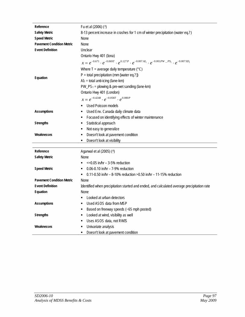
SD2006-10 Page 97 Analysis of MDSS Benefits & Costs May 2009
Reference Fu et al (2006) (3) Safety Metric 8-13 percent increase in crashes for 1 cm of winter precipitation (water eq.?) Speed Metric None Pavement Condition Metric None Event Definition Unclear
Equation
Ontario Hwy 401 (Iona) 111 007.0_001.0007.0127.0069.0671.0 SDPSPWAIPT eeeeeex −−−−− ⋅⋅⋅⋅⋅=
Where T = average daily temperature (°C) P = total precipitation (mm [water eq.?]) AI1 = total anti-icing (lane-km) PW_PS1 = plowing & pre-wet sanding (lane-km) Ontario Hwy 401 (London)
PT eeex 080.0058.04248.0 ⋅⋅= −−
Assumptions Used Poisson models Used Env. Canada daily climate data Focused on identifying effects of winter maintenance
Strengths Statistical approach
Weaknesses Not easy to generalize Doesn’t look at pavement condition Doesn’t look at visibility
Reference Agarwal et al (2005) (4) Safety Metric None
Speed Metric <=0.05 in/hr – 3-5% reduction 0.06-0.10 in/hr – 7-9% reduction 0.11-0.50 in/hr – 8-10% reduction >0.50 in/hr – 11-15% reduction
Pavement Condition Metric None Event Definition Identified when precipitation started and ended, and calculated average precipitation rate Equation None
Assumptions Looked at urban detectors Used ASOS data from MSP Based on freeway speeds (~65 mph posted)
Strengths Looked at wind, visibility as well
Weaknesses Uses ASOS data, not RWIS Univariate analysis Doesn’t look at pavement condition

SD2006-10 Page 98 Analysis of MDSS Benefits & Costs May 2009
Reference Eisenberg and Warner (2005) (5)
Safety Metric
On snow days… 24 percent increase in injury crashes 78 percent increase in PDO crashes on snow days 16 percent decrease in fatal crashes
Speed Metric None Pavement Condition Metric None
Event Definition Looked at daily weather data over a statewide level; “snow days” had 0.5 cm of reported snow
Equation Assumptions Poisson/ Gamma distribution Strengths Ease to understand statistic
Weaknesses Statewide scale causes problems of precision (i.e. California) Doesn’t look at pavement condition Doesn’t look at anything beside snowfall
Reference Zhang et al (2005) (6)
Safety Metric Crash rate is 53 percent higher when snowing than during non-precipitation conditions This percentage differed based on traffic volumes, but without a consistent trend
Speed Metric None Pavement Condition Metric None Event Definition An hour that included any precipitation and temperature was less than freezing
Equation
( )∑∑
=
v
Twv
v
Awv
Twv
Awv
vw HHHH
sRRR,,
,,,
Where AwvH , =number of hours with accidents when flow rate was v and weather was w
TwvH , =number of total hours with flow rate v and weather w
Assumptions
Precipitation measured from reflectivity, translated to rainfall; rain converted to snow based on airport temperature reading
Focused on freeway segments Used ATR data for traffic volumes
Strengths Easy to understand statistic
Weaknesses Not sensitive to snow amount Not certain that snow was observed Doesn’t look at pavement condition
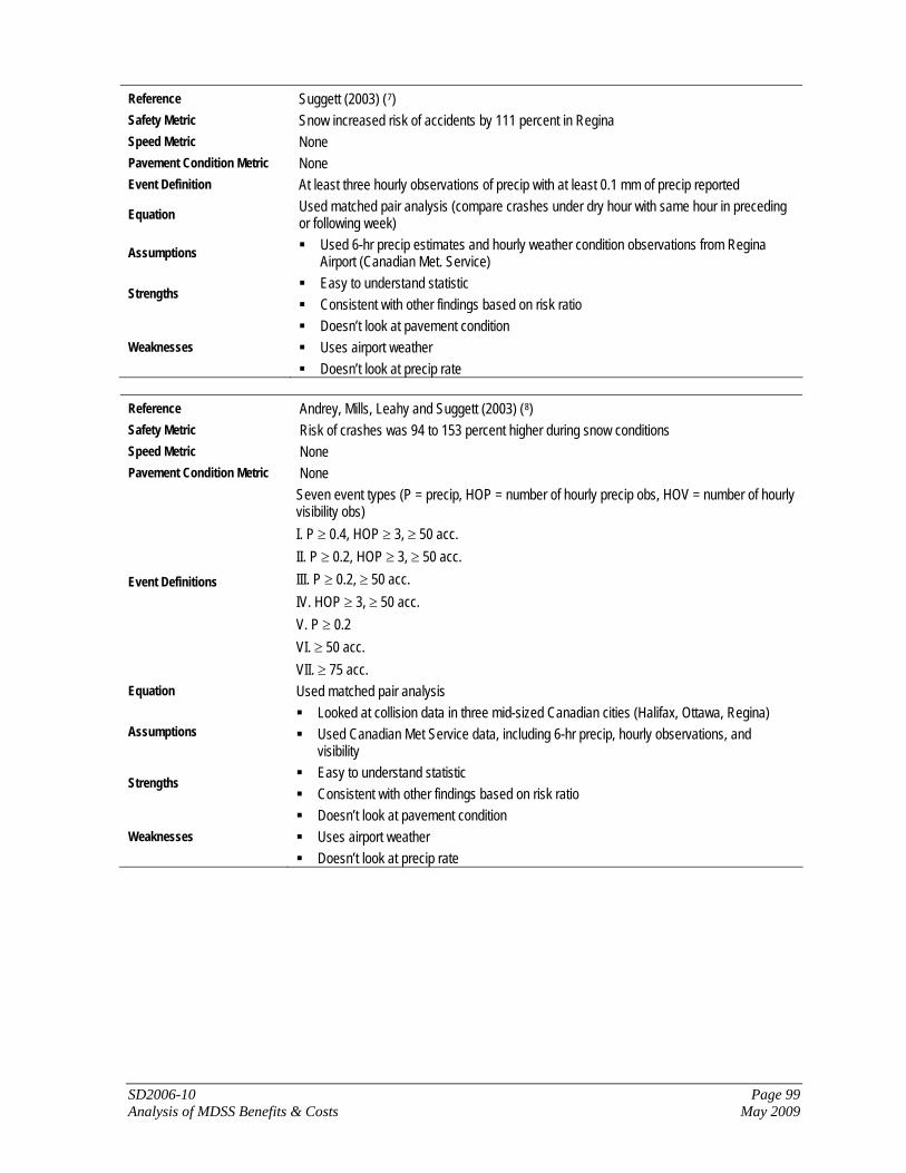
SD2006-10 Page 99 Analysis of MDSS Benefits & Costs May 2009
Reference Suggett (2003) (7) Safety Metric Snow increased risk of accidents by 111 percent in Regina Speed Metric None Pavement Condition Metric None Event Definition At least three hourly observations of precip with at least 0.1 mm of precip reported
Equation Used matched pair analysis (compare crashes under dry hour with same hour in preceding or following week)
Assumptions Used 6-hr precip estimates and hourly weather condition observations from Regina Airport (Canadian Met. Service)
Strengths Easy to understand statistic Consistent with other findings based on risk ratio
Weaknesses Doesn’t look at pavement condition Uses airport weather Doesn’t look at precip rate
Reference Andrey, Mills, Leahy and Suggett (2003) (8) Safety Metric Risk of crashes was 94 to 153 percent higher during snow conditions Speed Metric None Pavement Condition Metric None
Event Definitions
Seven event types (P = precip, HOP = number of hourly precip obs, HOV = number of hourly visibility obs) I. P ≥ 0.4, HOP ≥ 3, ≥ 50 acc. II. P ≥ 0.2, HOP ≥ 3, ≥ 50 acc. III. P ≥ 0.2, ≥ 50 acc. IV. HOP ≥ 3, ≥ 50 acc. V. P ≥ 0.2 VI. ≥ 50 acc. VII. ≥ 75 acc.
Equation Used matched pair analysis
Assumptions Looked at collision data in three mid-sized Canadian cities (Halifax, Ottawa, Regina) Used Canadian Met Service data, including 6-hr precip, hourly observations, and
visibility
Strengths Easy to understand statistic Consistent with other findings based on risk ratio
Weaknesses Doesn’t look at pavement condition Uses airport weather Doesn’t look at precip rate
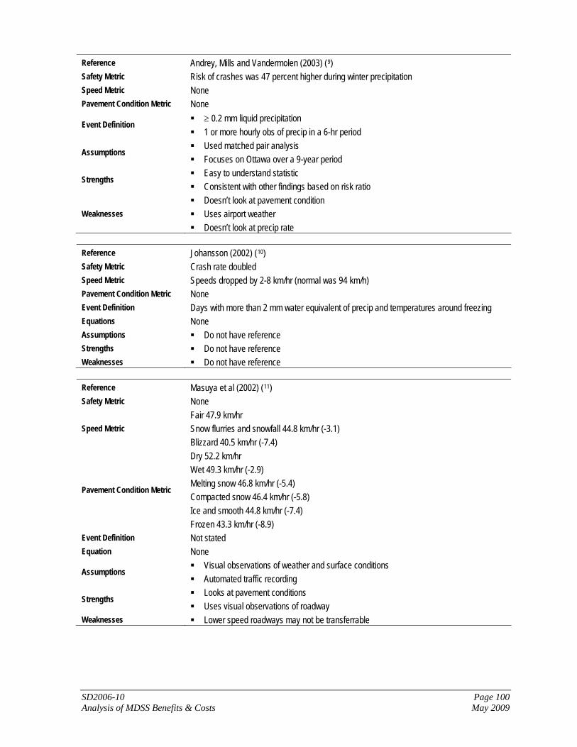
SD2006-10 Page 100 Analysis of MDSS Benefits & Costs May 2009
Reference Andrey, Mills and Vandermolen (2003) (9) Safety Metric Risk of crashes was 47 percent higher during winter precipitation Speed Metric None Pavement Condition Metric None
Event Definition ≥ 0.2 mm liquid precipitation 1 or more hourly obs of precip in a 6-hr period
Assumptions Used matched pair analysis Focuses on Ottawa over a 9-year period
Strengths Easy to understand statistic Consistent with other findings based on risk ratio
Weaknesses Doesn’t look at pavement condition Uses airport weather Doesn’t look at precip rate
Reference Johansson (2002) (10) Safety Metric Crash rate doubled Speed Metric Speeds dropped by 2-8 km/hr (normal was 94 km/h) Pavement Condition Metric None Event Definition Days with more than 2 mm water equivalent of precip and temperatures around freezing Equations None Assumptions Do not have reference Strengths Do not have reference Weaknesses Do not have reference Reference Masuya et al (2002) (11) Safety Metric None
Speed Metric Fair 47.9 km/hr Snow flurries and snowfall 44.8 km/hr (-3.1) Blizzard 40.5 km/hr (-7.4)
Pavement Condition Metric
Dry 52.2 km/hr Wet 49.3 km/hr (-2.9) Melting snow 46.8 km/hr (-5.4) Compacted snow 46.4 km/hr (-5.8) Ice and smooth 44.8 km/hr (-7.4) Frozen 43.3 km/hr (-8.9)
Event Definition Not stated Equation None
Assumptions Visual observations of weather and surface conditions Automated traffic recording
Strengths Looks at pavement conditions Uses visual observations of roadway
Weaknesses Lower speed roadways may not be transferrable

SD2006-10 Page 101 Analysis of MDSS Benefits & Costs May 2009
Reference Kyte et al (2001) (12) Safety Metric None Speed Metric 16.4 km/hr reduction in speeds when snow is on road Pavement Condition Metric 16.4 km/hr reduction in speeds when snow is on road Event Definition Not stated
Equation
WindVisWetSnowspeed 7.113.775.94.162.100 −+−−= Where Snow = whether snow is on road Wet = whether pavement is wet Vis = visibility (not to exceed .28km) Wind = whether wind > 24 km/hr
Assumptions Uses RWIS data Used rural freeway
Strengths Uses collocated RWIS and ATR data Uses a measure of pavement condition
Weaknesses One-day sample size Reference Perrin et al (2001) (13) Safety Metric None
Speed Metric
Wet – 10 percent decrease from dry speeds Wet and snowing – 13 percent decrease Wet and slushy – 25 percent decrease Slushy in wheel paths – 30 percent decrease
Pavement Condition Metric None
Event Definition Used seven weather conditions: dry, wet, wet and snowing, wet and slushy, slushy in wheel paths, snowy and sticking, snowing and packed (from 1977 FHWA study)
Equation None Assumptions Unclear Strengths
Weaknesses Unclear about how and where weather was observed Focuses on signalized intersections in urban context
Reference Transportation Research Board (2000) (14) Safety Metric None Speed Metric Estimates a 6 mph speed reduction in light snow, 31 mph reduction in heavy snow Pavement Condition Metric None Event Definition None Equation None Assumptions Based on other literature Strengths Standard reference
Weaknesses Purely atmospheric conditions Precip rates not defined
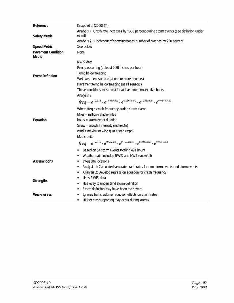
SD2006-10 Page 102 Analysis of MDSS Benefits & Costs May 2009
Reference Knapp et al (2000) (15)
Safety Metric Analysis 1: Crash rate increases by 1300 percent during storm events (see definition under event) Analysis 2: 1 inch/hour of snow increases number of crashes by 250 percent
Speed Metric See below Pavement Condition Metric
None
Event Definition
RWIS data Precip occurring (at least 0.20 inches per hour) Temp below freezing Wet pavement surface (at one or more sensors) Pavement temp below freezing (at all sensors) These conditions must exist for at least four consecutive hours
Equation
Analysis 2 windsnowhoursmiles eeeeefreq 0144.0255.1156.0098.1316.2 ⋅⋅⋅⋅= −
Where freq = crash frequency during storm event Miles = million-vehicle-miles hours = storm event duration Snow = snowfall intensity (inches/hr) wind = maximum wind gust speed (mph) Metric units
windsnowhourskm eeeeefreq 009.0494.0156.0682.0316.2 ⋅⋅⋅⋅= −
Assumptions
Based on 54 storm events totaling 491 hours Weather data included RWIS and NWS (snowfall) Interstate locations Analysis 1: Calculated separate crash rates for non-storm events and storm events Analysis 2: Develop regression equation for crash frequency
Strengths Uses RWIS data Has easy to understand storm definition
Weaknesses Storm definition may have been too severe Ignores traffic volume reduction effects on crash rates Higher crash reporting may occur during storms

SD2006-10 Page 103 Analysis of MDSS Benefits & Costs May 2009
Reference Knapp et al (2000) (15) Safety Metric None
Speed Metric 18.7 km/hr [11.6 mph] reduction in speeds when snow is on road that impacted travel lanes (from dry speed of 115.1 km/hr [71.5 mph])
Pavement Condition Metric 18.7 km/hr [11.6 mph] reduction in speeds when snow is on road that impacted travel lanes (from dry speed of 115.1 km/hr [71.5 mph])
Event Definition A sample of seven events was selected, for which data was collected real-time; events ranged from 5-6 inches of snow to no snow
Equation
6.8965.1125.600003.0 2 +−−= surfvisvolSpeed Where speed is km/hr vol = traffic volume Vis = visibility index (1 if vis < 0.4 km, 0 other) Surf = roadway surface condition index (percentage of road covered with snow) English units equation is
7.5523.788.300002.0 2 +−−= surfvisvolSpeed
Assumptions Used video data collection equipment to record road surface condition Looked at Interstate traffic
Strengths Uses pavement condition data Did both regression and simple comparative statistics
Weaknesses Didn’t look at interaction terms Didn’t distinguish snow and ice

SD2006-10 Page 104 Analysis of MDSS Benefits & Costs May 2009
Reference Kyte et al (2000) (16) Safety Metric None
Speed Metric 9.1-10.8 km/hr reduction in speeds when snow/ice is present on roadway (from 117 km/hr dry pavement speed)
Pavement Condition Metric 9.1-10.8 km/hr reduction in speeds when snow/ice is present on roadway (from 117 km/hr dry pavement speed)
Event Definition Normal speeds calculated on no precipitation, dry roadway, visibility greater than 0.37 km, wind speed less than 16 km/hr
Equation
Model 1 WindVisIntensPvmntspeed 34.062.077.454.48.115 −+−−=
Where speed is km/hr pvmnt = pavement condition (1 = dry, 2 = wet, 3 = snow/ice) intens = precip intensity (1 = none, 2 = light, 3 = medium, 4 = heavy) Vis = visibility (1 = <0.16 km, 2 = 0.16-0.37 km, 3 = >0.37 km) wind = wind speed (1 = 0-16 km/h, 2 = 16-32 km/h, 3 = 32-48 km/hr, 4 = >48 km/hr) Model 3
WindIntensPvmntspeed 03.974.843.55.126 −−−= wind = wind speed (1 = < 48 km/hr, 2 = >48 km/hr)
Assumptions Uses RWIS data, from two winters (1997-99) Used rural freeway
Strengths Uses collocated RWIS and ATR data Uses a measure of pavement condition
Weaknesses Doesn’t look at interaction terms Doesn’t verify accuracy of RWIS sensors

SD2006-10 Page 105 Analysis of MDSS Benefits & Costs May 2009
Reference Wallman (17) Safety Metric None
Speed Metric
Of 14 different pavement conditions, the following were average speed reductions Moist: 1 km/hr Wet: 2 km/hr Hoarfrost: 4 km/hr Black Ice: 5 km/hr Hard snow: 12 km/hr Soft snow: 10 km/hr Slush: 11 km/hr
Pavement Condition Metric
Of 14 different pavement conditions, the following were average speed reductions Moist: 1 km/hr Wet: 2 km/hr Hoarfrost: 4 km/hr Black Ice: 5 km/hr Hard snow: 12 km/hr Soft snow: 10 km/hr Slush: 11 km/hr
Event Definition Not defined (not clear how RWIS data was used)
Equation Used matched hour observations (match hours when only weather and surface conditions differed)
Assumptions Weather data included RWIS stations and road surface observations Five sites on low ADT (<3,500) roads with speed limits from 70-110 km/hr
Strengths Use of visual observations helps with pavement condition
Weaknesses Some variance in results by sites Doesn’t quantify how various surface observations correspond with objective measures
(i.e. % ice, snow depth)
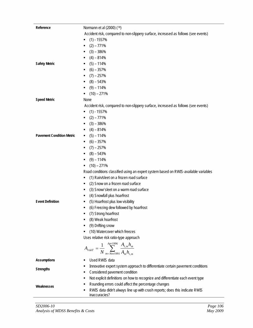
SD2006-10 Page 106 Analysis of MDSS Benefits & Costs May 2009
Reference Normann et al (2000) (18)
Safety Metric
Accident risk, compared to non-slippery surface, increased as follows (see events) (1) - 1557% (2) – 771% (3) – 386% (4) – 814% (5) – 114% (6) – 357% (7) – 257% (8) – 543% (9) – 114% (10) – 271%
Speed Metric None
Pavement Condition Metric
Accident risk, compared to non-slippery surface, increased as follows (see events) (1) - 1557% (2) – 771% (3) – 386% (4) – 814% (5) – 114% (6) – 357% (7) – 257% (8) – 543% (9) – 114% (10) – 271%
Event Definition
Road conditions classified using an expert system based on RWIS-available variables (1) Rain/sleet on a frozen road surface (2) Snow on a frozen road surface (3) Snow/ sleet on a warm road surface (4) Snowfall plus hoarfrost (5) Hoarfrost plus low visibility (6) Freezing dew followed by hoarfrost (7) Strong hoarfrost (8) Weak hoarfrost (9) Drifting snow (10) Watercover which freezes
Uses relative risk ratio-type approach
∑=
=1996
1991 ,
,1 Apr
Novm mtm
mmtriskT hA
hAN
A
Assumptions Used RWIS data
Strengths Innovative expert system approach to differentiate certain pavement conditions Considered pavement condition
Weaknesses
Not explicit definitions on how to recognize and differentiate each event type Rounding errors could affect the percentage changes RWIS data didn’t always line up with crash reports; does this indicate RWIS
inaccuracies?

SD2006-10 Page 107 Analysis of MDSS Benefits & Costs May 2009
Reference Maki (1999) (19) Safety Metric None Speed Metric Average speed dropped from 44 mph during “normal” to 26 mph during “adverse” conditions Pavement Condition Metric Indirectly Event Definition Adverse event is snowstorm with three or more inches of snow Equation None
Assumptions TH 36 in Twin Cities; signalized arterial Tried to use RWIS data, but was unsuccessful in correlating it with actual road conditions Used 2 normal, 3 adverse events
Strengths Clean storm definition
Weaknesses Unclear how snow depth measurements were conducted (wheel track? Total snowfall? Measured where?)
Reference Liang et al (1998) (20) Safety Metric None
Speed Metric Average speed reduction in snow events 19.2 km/hr (based on comparison across events) Average speed reduction for snow floor (regression) is 3.5 km/hr
Pavement Condition Metric Average speed reduction for snow floor (regression) is 3.5 km/hr
Event Definition Normal: sunny, clear, windless days Snow events are not defined
Equation
windtempdayfloorvisspeed 09.158.258.249.361.413.89 −++−+= Where speed is in km vis = logarithm of visibility (km) floor = indicator variable (1 = snow floor, 0 = dry) day = indicator variable (1 = daylight, 0 = night) temp = indicator variable (1 = temp > 0° C, 0 otherwise) wind = indicator variable (1 = wind > 40 km/hr, 0 otherwise)
Assumptions Rural freeway, speed limit 55 mph Strengths Easy to understand
Weaknesses
Low R2 (0.384) “Snow event” will include reduced visibility, perhaps wind and night, so it’s not a reliable
factor by itself Slipperiness of “snow floor” is undefined
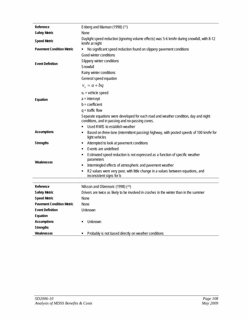
SD2006-10 Page 108 Analysis of MDSS Benefits & Costs May 2009
Reference Enberg and Mannan (1998) (21) Safety Metric None
Speed Metric Daylight speed reduction (ignoring volume effects) was 5-6 km/hr during snowfall, with 8-12 km/hr at night
Pavement Condition Metric No significant speed reduction found on slippery pavement conditions
Event Definition
Good winter conditions Slippery winter conditions Snowfall Rainy winter conditions
Equation
General speed equation bqavs +=
vs = vehicle speed a = intercept b = coefficient q = traffic flow Separate equations were developed for each road and weather condition, day and night conditions, and in passing and no-passing zones.
Assumptions Used RWIS to establish weather Based on three-lane (intermittent passing) highway, with posted speeds of 100 km/hr for
light vehicles Strengths Attempted to look at pavement conditions
Weaknesses
Events are undefined Estimated speed reduction is not expressed as a function of specific weather
parameters Intermingled effects of atmospheric and pavement weather R2 values were very poor, with little change in a values between equations, and
inconsistent signs for b Reference Nilsson and Obrenovic (1998) (22) Safety Metric Drivers are twice as likely to be involved in crashes in the winter than in the summer Speed Metric None Pavement Condition Metric None Event Definition Unknown Equation Assumptions Unknown Strengths Weaknesses Probably is not based directly on weather conditions

SD2006-10 Page 109 Analysis of MDSS Benefits & Costs May 2009
Reference Shankar et al (1995) (23) Safety Metric None Speed Metric 10-30 percent reduction in speeds during snow and ice conditions Pavement Condition Metric None Event Definition Looked at snowfall accumulations of >2 inches on a given day, and maximum daily snowfall Equation Negative binomial estimation of accident frequency involved more than a dozen variables Assumptions Strengths Weaknesses Looked at interactions between geometry and weather, not weather in isolation Reference Oeberg (1995) (24) Safety Metric None Speed Metric 10-30 percent reduction in speeds during snow and ice conditions Pavement Condition Metric None Event Definition Unknown Equation Assumptions Unknown Strengths Unknown Weaknesses Unknown Reference Ibrahim and Hall (1994) (25) Safety Metric None
Speed Metric Ignoring flow effects, speed reduction is 1-3 km/hr in light snow and 38-50 km/r in heavy snow
Pavement Condition Metric None Event Definition Used heavy and light snow (ranges were not discussed)
Equation
Used matched pair comparison method Median Lane (Station 14)
qddqspeed 12 23.05037.0114 −−−= Three-lane average (Station 14) – may include influence of slow-moving vehicles
qdqddqspeed 212 42.019.04143.0105 −−−−= Median Lane (Station 21)
21 35354.0101 ddqspeed −−−= Three-lane average (Station 21)
qdddqspeed 121 2.037164.0102 −−−−=
Assumptions Used airport weather Two sites on QEW in Ontario (urban application)
Strengths Oft referenced study
Weaknesses
Doesn’t define precip rates Limited number of events Interaction terms with traffic flow make it hard to isolate weather effects Doesn’t isolate pavement effects

SD2006-10 Page 110 Analysis of MDSS Benefits & Costs May 2009
Reference Andrey (1989) (26) Safety Metric 165 percent increase in crash rate in snowy conditions Speed Metric None Pavement Condition Metric None Event Definition Snowy (not defined) Equation Probably used matched pair analysis Assumptions Unknown Strengths Unknown
Weaknesses Unknown Didn’t look at pavement conditions Unpublished
Reference Mende (1982) (27) Safety Metric 30-140 percent increase in crash rates when significant snowfall occurs Speed Metric None Pavement Condition Metric None Event Definitions Significant snowfalls (not defined) Equation Assumptions Unknown Strengths Unknown
Weaknesses Unknown Didn’t look at pavement conditions Unpublished
Reference O’Leary (1978) (28) Safety Metric Crash rate increased up to 250 percent on snow vs. average days Speed Metric None Pavement Condition Metric None Event Definition Snow days (not defined) Equation Assumptions Unknown Strengths Unknown
Weaknesses Unknown Didn’t look at pavement conditions Unpublished
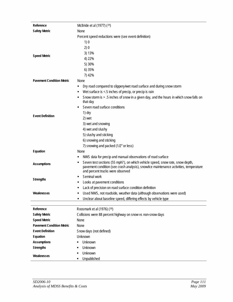
SD2006-10 Page 111 Analysis of MDSS Benefits & Costs May 2009
Reference McBride et al (1977) (29) Safety Metric None
Speed Metric
Percent speed reductions were (see event definition) 1) 0 2) 0 3) 13% 4) 22% 5) 30% 6) 35% 7) 42%
Pavement Condition Metric None
Event Definition
Dry road compared to slippery/wet road surface and during snow storm Wet surface is <.5 inches of precip, or precip is rain Snow storm is > .5 inches of snow in a given day, and the hours in which snow falls on
that day Seven road surface conditions
1) dry 2) wet 3) wet and snowing 4) wet and slushy 5) slushy and sticking 6) snowing and sticking 7) snowing and packed (1/2” or less)
Equation None
Assumptions
NWS data for precip and manual observations of road surface Seven test sections (55 mph?), on which vehicle speed, snow rate, snow depth,
pavement condition (see crash analysis), snow/ice maintenance activities, temperature and percent trucks were observed
Strengths Seminal work Looks at pavement conditions
Weaknesses Lack of precision on road surface condition definition Used NWS, not roadside, weather data (although observations were used) Unclear about baseline speed, differing effects by vehicle type
Reference Roosmark et al (1976) (30) Safety Metric Collisions were 88 percent highway on snow vs non-snow days Speed Metric None Pavement Condition Metric None Event Definition Snow days (not defined) Equation Unknown Assumptions Unknown Strengths Unknown
Weaknesses Unknown Unpublished
SD2006-10 Page 112 Analysis of MDSS Benefits & Costs May 2009
Reference OECD (1976) (31) Safety Metric Crash rate twice as high during snow as during normal conditions Speed Metric None Pavement Condition Metric None Event Definition Snowy conditions (not defined) Equation Unknown Assumptions Unknown
Strengths Unknown Might look at pavement conditions?
Weaknesses Unknown Unpublished
References 1. Hranac, R., E. Sterzin, D. Krechmer, H. Rakha, and M. Farzaneh, Empirical Studies on Traffic
Flow in Inclement Weather, Publication No. FHWA-HOP-07-073, Federal Highway Administration, U.S. Department of Transportation, October 2006.
2. Munehiro, K., N. Takahashi and M. Asano, “Using Probe-Car Data to Analyze Winter Road Traffic Performance in the Urban Sapporo Area,” Proceedings of the 5th International Symposium on Highway Capacity and Quality of Service, Japan Society of Traffic Engineers, July 2006, pp. 349-358.
3. Fu, L., M. Perchanok, L. Miranda-Moreno and Q. Shah, “Effects of Winter Weather and Maintenance Treatments on Highway Safety,” Proceedings of the 85th Annual Meeting of the Transportation Research Board, Transportation Research Board, Washington, DC, 2006.
4. Agrawal, M., T.H. Maze, and R. Souleyrette, Impact of Weather on Urban Freeway Traffic Flow Characteristics and Facility Capacity, Prepared for the Aurora consortium by the Center for Transportation Research and Education, Iowa State University, August 2005.
5. Eisenberg, D. and K. Warner, “Effects of Snowfalls on Motor Vehicle Collisions, Injuries, and Fatalities,” American Journal of Public Health, vol. 95, no. 1, January 2005, pp. 120-124.
6. Zhang, C., J.N. Ivan, W.M. ElDessouki, and E. Anagnostou, “Relative Risk Analysis for Studying the Impact of Adverse Weather Conditions and Congestion on Traffic Accidents,” Proceedings of the 84th Annual Meeting of the Transportation Research Board, Transportation Research Board, 2005.
7. Suggett, J., “Weather-Related Collisions in Regina, Saskatchewan,” in Andrey, J. and C. Knapper (eds.), Weather and Transportation in Canada, Department of Geography Series No. 55, University of Waterloo, Waterloo, Ontario, 2003.
8. Andrey, J., B. Mills, M. Leahy and J. Suggett, “Weather as a Chronic Hazard for Road Transportation in Canadian Cities,” Natural Hazards, vol. 28, 2003, pp. 319-343.
9. Andrey, J., B. Mills and J. Vandermolen, “A Temporal Analysis of Weather-Related Collision Risk for Ottawa, Canada: 1990-1998,” Proceedings of the 82nd Annual Meeting of the Transportation Research Board, Transportation Research Board, 2003.
10. Johansson, Ö, “Accidents, Speed and Salt Consumption on Roads in Winter,” Proceedings of the 11th International Winter Road Congress, World Road Association (PIARC), 2002.
11. Masuya, Y., K. Urata, N. Ito, T. Tamura and K. Saito, “Analysis of Winter Travel Speed in Pass Sections in Hokkaido,” Proceedings of the 11th International Winter Road Congress, World Road Association (PIARC), 2002.
SD2006-10 Page 113 Analysis of MDSS Benefits & Costs May 2009
12. Kyte, M., Z. Khatib, P. Shannon and F. Kitchener, “The Effect of Weather on Free Flow Speed,”
Transportation Research Record 1776, Transportation Research Board, Washington, DC, 2001, pp. 60-68
13. Perrin, J., P.T. Martin, and B.G. Hansen, “Modifying Signal Timing During Inclement Weather,” Transportation Research Record 1748, Transportation Research Board, Washington, DC, 2001, pp. 66-71.
14. Transportation Research Board, “Chapter 22: Freeway Facilities,” in Highway Capacity Manual, Transportation Research Board, Washington, DC, 2000.
15. Knapp, K.K., D. Kroeger and K. Giese, Mobility and Safety Impacts of Winter Storm Events in a Freeway Environment: Final Report, Center for Transportation Research and Education, Iowa State University, February 2000.
16. Kyte, M., Z. Khatib, P. Shannon and F. Kitchener, “Effect of Environmental Factors on Free-Flow Speed,” Proceedings of the Fourth International Symposium on Highway Capacity, June 27-July 1, 2000, Maui, Hawaii, Transportation Research Circular E-C018, Transportation Research Board, 2000, pp. 108-119.
17. Wallman, Carl-Gustaf, “Vehicle Speed and Flow at Various Winter Road Conditions,” Proceedings of the Ninth AASHTO/TRB Maintenance Management Conference, July 16-20, 2000, Juneau, Alaska, Transportation Research Board, Washington, DC, 2000.
18. Normann, J., M. Eriksson and S. Lindqvist, “Relationships between road slipperiness, traffic accident risk and winter road maintenance activity,” Climate Research, Vol. 15, 2000, pp. 185-193.
19. Maki, P.J., “Adverse Weather Traffic Signal Timing,” Proceedings of the 69th Annual Meeting of the Institute of Transportation Engineers, 1999.
20. Liang, W.L., M. Kyte, F. Kitchener and P. Shannon, “Effect of Environmental Factors on Driver Speed: A Case Study,” Transportation Research Record 1635, Transportation Research Board, Washington, DC, 1998, pp. 155-161.
21. Enberg, Å and S. Mannan, “Effects of Road and Weather Conditions on Traffic Flow on a Three-Lane Rural Highway in Finland,” Proceedings of the 10th PIARC International Winter Road Congress, March 16-19, 1998, Lulea Sweden, World Road Association (PIARC), pp. 1019-1032.
22. Nilsson, G. and A. Obrenovic, Road Accident Risk Twice as High in the Winter, Report No. 435, Swedish Road and Traffic Research Institute, 1998.
23. Shankar, V., F. Mannering and W. Barfield, “Effect of Roadway Geometrics and Environmental Factors on Rural Freeway Accident Frequencies,” Accident Analysis and Prevention, Vol. 27, No. 3, 1995, pp. 371-389.
24. Oeberg, Friction and Journey Speed on Roads with Various Winter Road Maintenance, VTI Report 237, Swedish Road and Traffic Research Institute (VTI), Linkoeping, Sweden, 1995. (Cited in Brown, K. and K. Baass, “Seasonal Variation in Frequencies and Rates of Highway Accidents as Function of Severity,” Transportation Research Record 1581, Transportation Research Board, Washington, DC, 1997, pp. 59-65.)
25. Ibrahim, A.T. and F.L. Hall, “Effect of Adverse Weather Conditions on Speed-Flow-Occupancy Relationships,” Transportation Research Record 1457, Transportation Research Board, Washington, DC, 1994, pp. 184-191.
26. Andrey, J., Relationships Between Weather and Traffic Safety, Unpublished Ph.D. dissertation, University of Waterloo, Waterloo, Ontario, 1989. (Cited in 7.)
27. Mende, I., An Analysis of Snowstorm-Related Accidents in Metropolitan Toronto, Master’s Thesis, Department of Civil Engineering, University of Toronto, Toronto, 1982. (Cited in 9.)
28. O’Leary, D., Some Impacts of Weather on Modern Transportation Systems: A Natural Hazards Approach, B.A. Thesis, Wilfrid Laurier University, Waterloo, Ontario, 1978. (Cited in Andrey, J., B. Mills and J. Vandermolen, Weather Information and Road Safety, Paper No. 15, Institute for Catastrophic Loss Reduction, Toronto, August 2001.)

SD2006-10 Page 114 Analysis of MDSS Benefits & Costs May 2009
29. McBride, J.C., W.J. Kennedy, J.H. Thuet, M.C. Belangie, R.M. Stewart, C.C. Sy and F.R.
McConkie, Economic Impact of Snow and Ice Control, FHWA Report No. FHWA-RD-77-95, Federal Highway Administration, Washington, DC, December 1977.
30. Roosmark, P.O., K. Anderson and G. Ahlquist, The effects of studded tyres on road accidents, National Swedish Road and Traffic Research Institute Report 72, Linkoeping, Sweden, 1976. (Cited in Andrey, J., B. Mills and J. Vandermolen, Weather Information and Road Safety, Paper No. 15, Institute for Catastrophic Loss Reduction, Toronto, August 2001.)
31. OECD (Organization for Economic Cooperation and Development), Adverse Weather, Reduced Visibility and Road Safety, OECD, Paris, 1976. (Cited in 9.)

SD2006-10 Page 115 Analysis of MDSS Benefits & Costs May 2009
Appendix E: Use of Posted Speed Limits The methodology assumes, for the purposes of delay calculation, that motorists will drive the posted speed limit unless winter weather conditions exist. In the absence of route-specific speed data, is this assumption reasonable? First, the research team did a brief scan of speed data collected by state DOTs to attempt to see how actual motorist speeds line up with posted speed limits. In general, these studies do not differentiate between good and bad weather conditions, so the reported average speed will likely underestimate the average speed that would be observed under ideal conditions. The 85th percentile speed – a speed compared to which 85 percent of motorists travel slower – is often used in highway design, and may be considered an upper bound to the average speed under ideal conditions for a given roadway type.
In a Washington state survey of several dozen sites for January-March 2006 (winter months), the average speed on 70 mph roadways was 69 mph; the 85th percentile speed (i.e. 85 percent of vehicles go slower than this speed) was 75 mph. On 65 mph roadways, the average speed was 59-62 mph, while the 85th percentile speed was 70-75 mph. It should be noted that there is considerable variation in adherence to speed limits for sites. Some sites reported more than 70 percent of traffic traveling in excess of the posted speed limit, while at other sites this was less than 20 percent.
The South Dakota speed monitoring report, for February 2007, showed average speeds of 73 mph on 75 mph roadways and 63 mph for 65 mph roadways. The 85th percentile speeds for these groups were 80 mph and 70 mph, respectively (i.e. 5 mph over the posted speed limit).
The data indicate that average speeds, counted over a variety of visibility, lighting and weather conditions, do line up reasonably well with posted speed limits. It is likely that average speeds during winter months for ideal weather conditions will be above the posted speed limit, perhaps by up to 5 mph. One potential alternative to the assumption that motorists follow the posted speed limit is to assume that the average travel speed during ideal conditions is 5 mph above the speed limit. This is perhaps a generous assumption based on the speed data above. Does this make a difference in delay calculations? The following sample calculations run through two examples: one where it is assumed that drivers were driving the posted speed limit (75 mph) and the other where they were not (80 mph). Speed reduction due to a winter storm event is estimated at 10 percent; use of MDSS would improve the pavement condition so that the average speed reduction is 5 percent. As shown in the calculations, motorist delay savings are overestimated if it is assumed that motorists drive more slowly (i.e. at the posted speed limit). However, the magnitude of overestimation is not that large even if it is assumed that there is a relatively large difference (5 mph) between the average driving speed and the posted limit. Moreover, because of longer hours of darkness and the potential for unexpected ice spots, it is likely that the difference between driving speeds and speed limits is lesser during the winter months. In addition, considerable variation has been observed in speed limit adherence for different highway segments. Given all these concerns, the research team does not believe it is appropriate to assume that motorists drive at higher average speeds than the posted speed limit.

SD2006-10 Page 116 Analysis of MDSS Benefits & Costs May 2009
Table 27: Delay at Posted Speed Limit & 5 mph Above
Example 1 Example 2 Average Speed =
Posted Speed Limit Average Speed =
5% Over Posted Speed Limit Normal Speed 75.0 mph 80.0 mph Lowered Speed (10% drop) 67.5 mph 72.0 mph MDSS Benefit: Lowered Speed (5% drop) 71.3 mph 76.0 mph Vehicle hours of travel – normal 666.7 veh-hrs 625.0 veh-hrs Vehicle hours of travel – without MDSS 740.7 veh-hrs 694.4 veh-hrs Vehicle hours of travel – with MDSS 701.8 veh-hrs 657.9 veh-hrs Delay without MDSS 74.0 veh-hrs 69.4 veh-hrs Delay with MDSS 35.1 veh-hrs 32.9 veh-hrs Delay savings due to MDSS 38.9 veh-hrs 36.5 veh-hrs Difference in Delay Estimate 2.4 veh-hrs Overestimation in Delay of… 6.6%
Assumptions Posted Speed Limit: 75 mph
Affected Traffic Volume 2,500 Vehicles Length of Segment 20 Miles
Affected VMT 50,000 VMT

SD2006-10 Page 117 Analysis of MDSS Benefits & Costs May 2009
Appendix F: Calculations of Delay Savings and Safety Benefits An extensive literature review (see Appendix D) turned up over 30 studies which have examined the impact of winter weather on traffic safety and/or vehicle speeds. These studies exhibit a wide variety of approaches and results. A detailed investigation revealed that the results of many of these studies may not be relevant to the current research project. First, many studies do not attempt to distinguish the effects of the weather’s effects on the pavement and the effects on driver perception. This is critical for this present study, since while the use of MDSS recommendations may affect the resulting condition of the pavement, it will have no impact on the perceptual effects of falling or blowing snow. In addition, many studies relied on National Weather Service-type observations which were collected some distance away from the roadway environment. There is also considerable variance in how different winter weather events are characterized or defined. Therefore, the team focused on the few studies which specifically examined the effects of pavement surface condition on safety and speed. The team used these studies to provisionally estimate the percentage increases in crash rate or decreases in speed associated with worsening pavement conditions. These percentages were associated with MDSS-generated descriptors of pavement condition, in order to make it easier to incorporate MDSS simulation output. The calculation of delay savings and safety benefits depends on knowing how the level of service will change between the Baseline and MDSS implementation scenarios. The output from MDSS can be used to calculate the number of hours at which a route segment i is operating at a given level of service n. For simplicity, the research team plans to define LOS according to the pavement condition estimated by MDSS. The number of hours at each level of service for a given route segment i can be calculated as an output from MDSS, as shown symbolically in the following table:
LOS Condition Baseline MDSS
(Same Conditions) MDSS
(Same Resources) 1 hrs1Bi hrs1Ci hrs1Ri 2 hrs2Bi hrs2Ci hrs2Ri 3 hrs3Bi hrs3Ci hrs3Ri : : : : N hrsnBi hrsnCi hrsnRi
Delay Benefits The values for hrsLXi (where L = level of service and X = scenario) represent a measure of exposure to various roadway levels of service. To compute the delay savings, this value must be translated into a measure of exposure related to vehicle traffic. Vehicle traffic volumes will vary throughout the day, and will also vary from weekdays to weekends. Consequently, the most precise way of measuring this exposure would be to have hourly traffic volume counts for each route segment in each case study state. Since such data do not exist, it is necessary to make some simplifying assumptions. First, it is assumed that winter storm events may occur at equal frequency at any time of the day. Second, it is assumed that winter storm events are equally likely to occur on any day of the week. If the timing of storm events is uniformly distributed like this, one may assume that traffic volumes are evenly distributed throughout the day. This means that the annual average daily traffic (AADT) volume can be used to determine hourly traffic volumes. Exposure to vehicle traffic can be calculated by converting an AADT value for route segment i into the average number of vehicle-hours spent on a route segment in a given hour. This can be done as follows:

SD2006-10 Page 118 Analysis of MDSS Benefits & Costs May 2009
24
iii
wAADTVH
×=
where VHi = the average number of vehicles per hour on route segment i AADTi = the average annual daily traffic volume for route segment i wi = the seasonal traffic volume adjustment factor for route segment i
AADT values (2006) for Colorado were obtained from the Colorado Department of Transportation web site (1). This data set also included 20-year growth factors to estimate traffic volumes in future years, as well as average daily truck traffic volumes. These factors were applied to estimate traffic volumes in earlier years 1 . In addition, this data set included AADT values for Minnesota were extracted from GIS data sets available on the Minnesota Department of Transportation’s web site (2). The underlying data set included historic and current traffic volumes (both for all traffic and for trucks). Seasonal adjustment factors for each state were calculated based on an examination of monthly traffic variation at automatic traffic recorder sites. The general process was to take a twelve-month period from July to June, calculated the average daily traffic volume in the winter months (i.e. November through March), and divide it by the average daily traffic over the entire twelve-month period. This generated a seasonal adjustment factor for each site. Traffic count data were collected from 108 sites in Colorado (1), 72 sites in Minnesota (3), and 62 sites in New Hampshire (4). The seasonal adjustment factors for all valid sites (i.e. all sites with at least one 12-month July-to-June period with no missing observations) were averaged, resulting in the following statewide seasonal adjustment factors:
Colorado: 0.891 (i.e. the daily traffic volume during the winter months is 89.1 percent of the daily traffic volume in a given year)
Minnesota: 0.897 New Hampshire: 0.913
This leaves the number of vehicles exposed to each level of service as follows:
LOS Condition BaselineMDSS
(Same Conditions)MDSS
(Same Resources) 1 VHihrs1Bi VHihrs1Ci VHihrs1Ri 2 VHihrs2Bi VHihrs2Ci VHihrs2Ri 3 VHihrs3Bi VHihrs3Ci VHihrs3Ri : : : : n VHihrsnBi VHihrsnCi VHihrsnRi
The travel speed associated with a given LOS can be calculated as a percentage of the posted speed limit for a given route segment i. These percentages will be expressed as a series of factors, vl for each level of service l:
LOS Condition Factor Adj. Speed 1 v1 (=1) viv1 2 v2 viv2 3 v3 viv3 : : : n vn vivn
1 Traffic volumes for non-trucks and trucks were counted separately for each state, in order to incorporate the higher value of travel time for trucks.

SD2006-10 Page 119 Analysis of MDSS Benefits & Costs May 2009
Based on the results of the literature review, the following factors were used in the analysis: LOS Condition Factor Adj. Speed
Dry 1 vi Wet 0.96 0.96vi
Chemically Wet 0.96 0.96vi Damp 1.00 vi
Lightly Slushy 0.90 0.90vi Slushy 0.87 0.87vi
Deep Slushy 0.84 0.84vi Dusting of Snow 0.96 0.96vi
Frost 0.94 0.94vi Lightly Icy 0.94 0.94vi
Icy 0.85 0.85vi Very icy 0.83 0.83vi
Lightly Snow-covered 0.89 0.89vi Snow-covered 0.84 0.84vi
If lengthi is the length of route segment i in miles, then the total travel time savings resulting from MDSS, as compared to the baseline case, is:
∑∑==
×−
×=Δ
F
AL Li
iLMiiF
AL Li
iLBii
vvlengthhrsVH
vvlengthhrsVH
delay
A positive value will indicate travel time savings as a result of MDSS; a negative value will indicate an increase in travel time.
Safety Benefits The calculation of safety benefits depends on a similar approach as delay savings. The approach is to assume that there is a certain crash rate associated with a particular highway facility, and that this crash rate increases proportionally as level of service deteriorates.
LOS Factor Crash Rate A cA (=1) cicA B cB cicB C cC cicC D cD cicD E cE cicE F cF cicF
where ci = the baseline crash rate for a given route segment i cL = a crash rate adjustment factor for level of service L The crash rate adjustment factors cL will be determined through a review of the literature. The main question, then, is how to calculate ci. The results of the MDSS simulation activities for the baseline case will be essential in filling this gap. For a given route segment i, the actual crash rate will be calculated using five winters of crash data as follows:
i
ii VMT
crashesc =
The percentage of time when the route segment is operating under each level of service is calculated for the baseline condition. Using the baseline crash rate ci and the crash adjustment factors cL, the expected number of crashes for each level of service are estimated as follows.
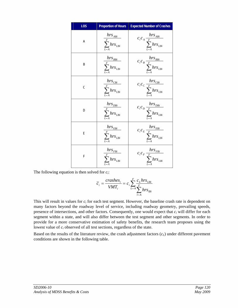
SD2006-10 Page 120 Analysis of MDSS Benefits & Costs May 2009
LOS Proportion of Hours Expected Number of Crashes
A ∑=
F
ALLBi
ABi
hrs
hrs
∑=
F
ALLBi
ABiAi
hrs
hrscc
B ∑=
F
ALLBi
BBi
hrs
hrs
∑=
F
ALLBi
BBiBi
hrs
hrscc
C ∑=
F
ALLBi
CBi
hrs
hrs
∑=
F
ALLBi
CBiCi
hrs
hrscc
D ∑=
F
ALLBi
DBi
hrs
hrs
∑=
F
ALLBi
DBiDi
hrs
hrscc
E ∑=
F
ALLBi
EBi
hrs
hrs
∑=
F
ALLBi
EBiEi
hrs
hrscc
F ∑=
F
ALLBi
FBi
hrs
hrs
∑=
F
ALLBi
FBiFi
hrs
hrscc
The following equation is then solved for ci:
∑∑=
=
==F
ALF
AllBi
LBiLi
i
ii
hrs
hrscc
VMTcrashes
c
This will result in values for ci for each test segment. However, the baseline crash rate is dependent on many factors beyond the roadway level of service, including roadway geometry, prevailing speeds, presence of intersections, and other factors. Consequently, one would expect that ci will differ for each segment within a state, and will also differ between the test segment and other segments. In order to provide for a more conservative estimation of safety benefits, the research team proposes using the lowest value of ci observed of all test sections, regardless of the state. Based on the results of the literature review, the crash adjustment factors (cL) under different pavement conditions are shown in the following table.

SD2006-10 Page 121 Analysis of MDSS Benefits & Costs May 2009
LOS Condition Crash Adjustment
Factor (%) Dry 100 Wet 150
Chemically Wet 150 Damp 100
Lightly Slushy 150 Slushy 175
Deep Slushy 200 Dusting of Snow 150
Frost 370 Lightly Icy 200
Icy 800 Very icy 1600
Lightly Snow-covered 210 Snow-covered 870
References 1. “Traffic Data,” Colorado Department of Transportation Web Page, Accessed at
http://www.dot.state.co.us/App_DTD_DataAccess/Traffic/index.cfm?fuseaction=TrafficMain&MenuType=Traffic on March 28, 2007.
2. “Statewide Base Map Data,” Minnesota Department of Transportation Web Page, Accessed at http://www.dot.state.mn.us/maps/gisbase/html/statewide.html on January 3, 2008.
3. “Automatic Traffic Recorder,” Minnesota Department of Transportation Web Page, Accessed at http://www.dot.state.mn.us/traffic/data/atr/atr.html on January 4, 2008.
4. “NHDOT – Business Center,” New Hampshire Department of Transportation Web Page, Accessed at http://www.nh.gov/dot/transportationplanning/traffic/index.htm#atr on January 4, 2008.

SD2006-10 Page 122 Analysis of MDSS Benefits & Costs May 2009
Appendix H: Definition of Alternatives The benefit-cost analysis is based on using MDSS as a simulation tool to compare a Base Case, in which an agency follows its standard rules of practice, with two MDSS implementation scenarios (Same Condition and Same Resources) which assume full use of MDSS treatment recommendations. These two full use scenarios include use of both Applications 1 (real-time integration of weather information) and 2 (adherence to MDSS treatment recommendations). The MDSS use options outlined in Section 3.4 (MDSS options) may reduce the benefits that could be realized from MDSS. Therefore, it is important to discuss how more “realistic” MDSS use scenarios will be developed from the outputs of the simulation approach.
Selection of Forecasting Services and Forecast Accuracy One potential option for MDSS implementation includes the ability for a state to use two vendors: one for procuring weather forecasting services, and another for support of the MDSS GUI and application. One would expect there to be a correlation between perceived forecast accuracy and use of MDSS. Consequently, to the extent that different forecasting services are perceived to offer different levels of accuracy in their forecasting services, one would expect to see varying levels of user acceptance of treatment recommendations provided by MDSS. Certainly forecast quality is an important consideration, and forecast accuracy should be considered for agencies procuring weather forecasting services. However, while forecast accuracy is an important element to consider in MDSS implementation, it was beyond the scope of this research project to assess the quality of different forecasting services which may be used as input into MDSS. Therefore, the use of a different vendor for providing weather forecasting services will not be considered as a different implementation option with different benefits and costs. Moreover, the use of weather forecasting services is not only for MDSS. States that do not use MDSS also purchase weather forecast services for winter maintenance. A related consideration is how MDSS responds to an inaccurate forecast. MDSS presumes that the weather forecasts received as input are accurate with respect to timing, duration and severity of winter weather events. By analogy, it is helpful to consider how human actors respond to inaccurate forecasts. One could envision two general types of missed forecasts: a false positive, when a predicted storm does not materialize to the extent or severity as predicted; and a false negative, when a storm is more severe than forecast (or perhaps was not forecast at all). The consequences of these types of missed forecasts are not equivalent. The false negative is especially perilous, because the agency must try to catch up to the event, and in the meantime the roadway level of service is degraded. A false positive means a “waste” of resources, which, though not optimal, is at least not unsafe. Because of the asymmetric consequences associated with false positives and false negatives, agencies often exercise extra caution in winter maintenance, using more chemicals than needed “just in case.” While human operators make decisions in this way, MDSS recommendations are based on a more precise modeling of the exact effort required to achieve a certain level of service. MDSS does not make allowances “just in case” forecasts are wrong. While human decision-makers are “better” than MDSS in being more flexible with respect to the uncertainty of forecasts, MDSS is “better” in its ability to synthesize weather information and make real-time adjustments as conditions change. MDSS is efficient at synthesizing input on current weather conditions, in combination with frequently updated forecasts, to provide course corrections as needed. Therefore, if there are bad forecasts, it could be said that MDSS is more agile to respond with appropriate recommendations as weather conditions evolve. Another important point is that it is logical to presume that the quality of forecasts used as inputs in MDSS is not inferior to the quality of forecasts obtained through other sources. In other words, it is

SD2006-10 Page 123 Analysis of MDSS Benefits & Costs May 2009
probably better to assume that there is no difference in forecast quality between MDSS and non-MDSS sources. Under this assumption, maintenance personnel always have to deal with the uncertainty associated with weather forecasts, and MDSS should not be assumed to either increase or reduce that uncertainty. In summary, forecast reliability and accuracy are relevant in understanding and quantifying the benefit of MDSS. However, the complexity of issues associated with these, which have only been lightly explored, make it impossible to effectively and reliably quantify them. Consequently, the analysis does not introduce alternatives that factor in variations in forecast accuracy or quality.
Consistency of Feedback on Actual Maintenance Operations MDSS assumes perfect feedback regarding the timing and nature of maintenance treatment actions. When operational, MDC is the only perfectly reliable way to provide continuous feedback to MDSS regarding maintenance actions that have been performed. MDC implementation among the pooled fund states has proceeded gradually, due to cost and technical concerns. In the absence of MDC, agency users would be required to use manual feedback to ensure that MDSS is making accurate recommendations. Manual feedback methods have had varying levels of success. Some maintenance personnel may be less diligent in providing feedback, since they don’t understand its value. During high-intensity storms, this feedback may also be regarded as less important than tending to snow-fighting operations, so there could be a growing gap between the actual and predicted condition of the roadway. Inaccuracy in reporting could cause MDSS to make prediction and treatment errors that are inconsistent in their direction, and thus could not be readily modeled in this benefit-cost analysis. Two examples may be offered. In one case, assume that an agency uses more chemicals than recommended by MDSS. This could result in MDSS appearing to be pessimistic about the pavement condition. MDSS would operate on this errant assumption about the condition of the pavement, and likely recommend more chemicals than needed on subsequent treatments. In another case, suppose that an agency does not execute a treatment action as quickly as recommended by MDSS. MDSS then presumes the pavement condition is better than it truly is, which means that MDSS might recommend less chemical or treatment than needed. It would be ideal if MDSS contained the means to degrade the feedback mechanism to more closely replicate the experiences of agencies relying on manual reporting, or on MDC platforms that are not fault-proof. This would make it easier to see the actual benefits of MDSS use based on real use environments experienced by MDSS agency users. This could allow for a comparison of implementation alternatives with and without MDC, which certainly could be an important investment decision for many agencies considering use of MDSS. However, the MDSS software affords no clean or reliable way of degrading the feedback. Revising the software to incorporate this type of functionality, even if it were possible, would not enhance MDSS’ utility to agency users in any meaningful way. Because of the inconsistent effects of bad feedback on MDSS “behavior,” the analysis assumes that feedback is perfect. To obtain this perfect feedback, the analysis assumes that agencies will deploy MDC. This is not an unreasonable assumption in that most pooled fund agencies have been experimenting with MDC and also hope for broader fleet-wide implementation of MDC/AVL platforms on their winter maintenance vehicles. One can reliably quantify the agency cost savings associated with not implementing MDC; however, one cannot reliably estimate the increased resource costs or degraded level of service that may result.

SD2006-10 Page 124 Analysis of MDSS Benefits & Costs May 2009
Use of Treatment Recommendations Several pooled fund states use MDSS primarily for Application 1 (real-time integration of weather information to forecast road conditions) and do not report using treatment recommendations; i.e. they do not use MDSS Application 2. Technically, unless MDSS results in a change in winter treatment actions, there will be no savings in winter maintenance costs, and no improvement in level of service. Consequently, there would be no tangible benefits for an agency implementing MDSS unless there is some use of Application 2. It is hypothesized that the agencies which do not report using MDSS for Application 2 are nonetheless influenced by the treatment recommendations; otherwise, they likely would not plan on investing in MDSS. Therefore, the research team assumes that an agency will change its treatment approach in response to MDSS. The agency may adapt its treatment approach based on MDSS treatment recommendations in a limitless number of ways, which could introduce considerable complexity into the analysis. For simplicity, it is assumed that agencies may selectively use MDSS recommendations in one of two ways. In some cases, agency use of MDSS recommendations could appear to be somewhat random, as it is based on the preferences and biases of the maintenance supervisor and personnel at a local shed. Alternatively, agencies may consistently use MDSS to respond to certain types of storm events, but not to others. Based on outreach to pooled fund states, the research team believes that the first way is closest to replicating the experience of pooled fund states. To simplify analysis, the research team proposes two levels of adherence to MDSS recommendations: full adherence and a percentage value (e.g., X=50 percent) adherence for a specific case study state. Under full adherence, the agency follows MDSS treatment recommendations exactly, even if those recommendations fall outside of the range of normal rules of practice. For the latter case, a state may sometimes follow the treatment recommendations exactly, but will sometimes ignore or modify treatment recommendations based on their judgment. As is discussed elsewhere in this document, the analysis regards the benefits of MDSS as being realized on a storm-by-storm or event-by-event basis. The resources used in each event can be summed to indicate the total volume of resources used. The hours of exposure to various levels of service can also be summed to indicate the total number of hours during a winter season under each pavement condition. If it is assumed that an agency uses treatment recommendations randomly, then one can simply dampen the benefits of MDSS by (1-X) percent.
Use of In-vehicle Graphical User Interface (GUI) The preceding MDSS implementation option dealt with the level of trust agencies put in MDSS recommendations. This final MDSS implementation option, the use of an in-vehicle graphical user interface (GUI), reflects the extent to which recommendations are seamlessly communicated to vehicle operators. If there is perfect communication between the MDSS platform and the vehicle operator implementing recommendations, then the recommendations can be implemented perfectly. If there is “friction” in the communication so that the recommendation does not reach the operator in a timely fashion, then the recommendations cannot be implemented perfectly. An in-vehicle GUI provides a means of preserving the chain of communication between MDSS and the vehicle operator. The in-vehicle GUI can provide information on current weather conditions, along with updated treatment recommendations, to help an operator effectively follow the recommended treatment. The in-vehicle GUI directly targets the vehicle operator, whereas the typical client-based MDSS desktop application may be only accessed by a maintenance manager. Without an in-vehicle GUI, the vehicle operator may be dependent on guidance that is one or two hours old; or, the vehicle operator may have no guidance from MDSS at all.
SD2006-10 Page 125 Analysis of MDSS Benefits & Costs May 2009
In order to clarify the effect of the in-vehicle GUI, it is important to recognize that MDSS is, by definition, a decision support tool. MDSS is intended to help inform decisions which are made regarding winter maintenance operations. Therefore, the assumption is that the recommendations which are generated by MDSS are communicated to those who are ultimately responsible for executing them; i.e. the vehicle operators. The execution of MDSS recommendations is ultimately related to user acceptance, and was addressed under the previous section. In considering the question of the effects of an in-vehicle GUI, the communication of recommendations is the key component. There may be two basic reasons why a treatment recommendation will not be communicated to the vehicle operator: user acceptance/trust, and a variety of technical issues. Under the first reason, one could envision a maintenance supervisor who is being forced to use MDSS but generally distrusts the program and its philosophy, and therefore refuses to pay heed to its recommendations. This, again, is an execution issue. The second reason, related to technical issues, is very pertinent. This could occur when a vehicle operator may not have access to a computer to view MDSS recommendations, whether at the maintenance yard or not; or if they are unable to receive recommendations from the supervisor’s computer, perhaps because the supervisor is away from the office. If a maintenance manager is supportive of considering MDSS recommendations, they will likely work to ensure that there is some communication of MDSS recommendations in the office environment. The in-vehicle GUI would offer improvements by allowing for mid-course corrections: adjustment of application rates, or perhaps even diversion to other routes within a shed’s coverage area. However, the in-vehicle GUI is not necessary for this to occur; a good radio system could work as well. In this research study, it is assumed that all plow trucks are installed with MDC that can provide a “perfect” feedback mechanism. GUI/AVL implementations are not considered for benefit-cost analysis.

SD2006-10 Page 126 Analysis of MDSS Benefits & Costs May 2009
Appendix H: Storm Classification An important supporting piece in this analysis is the normalization of weather. To recap, the simulation approach seeks to use several seasons of weather data to estimated benefits resulting from MDSS use compared to a Baseline condition. Two challenges arise from this. First, it is unclear whether the years of data used for a case study site are representative of longer-term climatic trends for that area. Second, there needs to be a way of translating the benefits identified at the case study sites to other sites in each state which, though they may employ identical rules of practice, are likely confronted with different winter weather conditions. The research team proposes using a storm-based analysis approach for dealing with both of these challenges. The idea is that each winter’s weather for a given site can be subdivided into a series of storm events. MDSS and Baseline maintenance practices can be compared for each storm. Then, the impacts associated with each storm can be multiplied by the normal storm frequencies for each location, to develop estimates of benefits for each site. A storm event is when there is at least 1 recorded hour of moisture, either as precipitation or condensation, on the roadway. This definition could include rain events, as well as dew or frost; not all storm events will require a winter maintenance response. One storm event is distinguished from another when there are at least six (6) consecutive hours of no moisture activity. Storms will be defined by looking at hourly observations of the following weather parameters:
Air temperature Precipitation rate or accumulation (convert as needed) Wind speed Relative humidity
The following steps need to be taken to ensure sufficient weather data to define storms: Interpolate air temperature for missing observations using linear interpolation between values
observed immediately before and after Interpolate relative humidity for missing observations using linear interpolation between values
observed immediately before and after Interpolate precipitation rate/accumulation between values observed immediately before and
after Interpolate average wind speed as numerical average (not vector) between values observed
immediately before and after Each event will be initially classified by the characteristics shown in Table 28. To define events, hourly weather observational data14 are read into and processed by Matlab. Missing hourly values are interpolated, weather parameter values are calculated, and the number of each type of event is counted for each winter season (November 1-March 31). A large number of potential events may be classified under this concept. There may 15,552 possible types of precipitation events (assumes 4 values of Trange, 3 values of Ttrend, 6 values of D, 4 non-zero values of Pacc, 3 non-zero values of Prate, 3 values of Wstorm, 2 values of Wpost, and 2 values of C) and 72 possible types of frost events (assumes Trange < 4, 3 values of Ttrend, 6 values of D, Pacc = Prate = 0, Wstorm = 0, 2 values of Wpost, and C = 1. Further analysis will be needed to identify clusters of storm events to consolidate these different classes of storms.
14 Up to 30 years of data collected from the National Climatic Data Center will be used, where available. In some cases, fewer years will be available.

SD2006-10 Page 127 Analysis of MDSS Benefits & Costs May 2009
The goal of this classification and consolidation approach is to develop a set of 20 or fewer storm types. The classification scheme for storms is used covering all case study states, to maximize transferability of results to other pooled fund states. By classification of historic weather data from a variety of locations within each case study state, and by identifying the weather site most likely representative of a given route segment’s weather, it will be possible to develop a climate profile for each route segment, as a distribution of the average frequency of various types of storm events:
Segment Type 1 Type 2 Type 3 … Type k Segment 1 1 4 5 … 0 Segment 2 0 3 6 … 1 Segment 3 1 5 9 … 1
Due to the large number of potential events with different parameter values under this concept, storms events need to be further classified into a certain number of groups. Cluster analysis method can be used for this purpose. While there are many existing techniques for cluster analysis, the k-means method15 is used in this study as it is more suitable for cluster analysis when the sample size is large (e.g., >200). K-means is a simple procedure to classify a given dataset through a certain number of clusters (assume k clusters). The algorithm of k-means aims at minimizing an objective function. The objective function is
∑∑= =
−=k
j
n
ij
ji cxJ
1 1
2
where 2
jj
i cx − is a distance measure between a data point jix and the cluster center jc , and J is an
indicator of the distance (squared Euclidean distance) of the n data points from their respective cluster centers. Storm frequency for weather data at the MDSS-simulated sites will be similarly analyzed. The purpose of this analysis is not to determine normal climatic conditions, but rather to estimate the average resource use and level of service results for each storm type under MDSS and Baseline conditions. These will be averaged over all storms of a given type for all areas with the same rules of practice in a given state. These per-storm estimates of benefits and level of service effects can then be applied to the normal frequencies of storm events for each location.
15 MacQueen, J.B. Some Methods for classification and Analysis of Multivariate Observations, Proceedings of 5-th Berkeley Symposium on Mathematical Statistics and Probability, Berkeley, University of California Press, 1:281-297, 1967.

SD2006-10 Page 128 Analysis of MDSS Benefits & Costs May 2009
Table 28 : Weather Parameter Values for Classifying Storms
Parameter How Collected Range Value Warm: 32° F < temperature range Trange = 4 Mid range: 25° F < temperature range <= 32° F Trange = 3 Cool: 15° F < temperature range <= 25° F Trange = 2
Air temperature range (Trange)
This will be based on the average of air temperature observations collected during the storm.
Cold: temperature range <= 15° F Trange = 1 Warming: (end temp.) – (beginning temp.) > 2° F Ttrend = 3 Steady: 2° F >= (end temp.) – (beginning temp.) >= -2° F
Ttrend = 2 Pavement
temperature trend (Ttrend)
This will be based on the difference between the temperature at the beginning and end of the storm events.
Cooling: (end temp.) – (beginning temp.) < -2° F Ttrend = 1 1-2 hours D = 1 3-4 hours D = 2 5-8 hours D = 3 9-12 hours D = 4 13-24 hours D = 5
Duration (D) This is the number of hours included in the storm event.
Over 24 hours D = 6 No accumulation Pacc = 0 0 < Accumulation < 0.1 inches Pacc = 1 0.1 <= Accumulation < 0.25 inches Pacc = 2 0.25 <= Accumulation < 0.50 inches Pacc = 3
Precipitation accumulation
(Pacc)
This is the sum of water equivalent precipitation encountered during the storm.
0> 0.50 inches Pacc = 4 No precipitation rate Prate = 0 0 < Rate < 0.05 inches/hr Prate = 1 0.05 inches/hr <= rate <= 0.10 inches/hr Prate = 2
Precipitation rate (Prate) This is the quotient of Pacc over D
0.10 inches/hr < rate Prate = 3 Wind speed < 2 mph Wstorm = 0 2 mph <= Wind speed <= 10 mph Wstorm = 1
Average wind speed in storm
(Wstorm) This is the average wind speed observation during the storm Over 10 mph Wstorm = 2
Wind speed <= 10 mph Wpost = 1 Average wind speed after
storm (Wpost)
This is the average wind speed observation during the 4 hours after the storm
Wind speed > 10 mph Wpost = 2
(Air temperature) – (Dewpoint/Frostpoint) > 2° F C = 0 Condensation (C)
This refers to whether the ambient temperature is equal to the dewpoint (Air temperature) – (Dewpoint/Frostpoint) <= 2° F C = 1

SD2006-10 Page 129 Analysis of MDSS Benefits & Costs May 2009
Appendix I: Weather Station and Availability of Data
State USAF-
WBAN_ID Station Name Latitude Longitude Elevation
(ft)
At Least 75%*
Less Than 75%**
Grand Total***
726040 99999 FRANCONIA 44.217 -71.75 942 1 3 4 726050 14745 CONCORD MUNICIPAL ARPT 43.195 -71.50 346 30 0 30 726055 99999 PEASE INTL TRADEPOR 43.083 -70.82 102 29 1 30 726116 94765 LEBANON MUNICIPAL 43.626 -72.31 570 20 10 30 726130 99999 MOUNT WASHINGTON 44.267 -71.30 6,266 9 21 30 726155 99999 LACONIA MUNI (AWOS) 43.567 -71.42 545 12 18 30 726160 99999 BERLIN MUNICIPAL 44.583 -71.18 1,158 10 2 12 726163 99999 JAFFREY MUNICIPAL 42.8 -72.00 1,040 9 1 10 726164 99999 WHITEFIELD 44.367 -71.55 1,073 7 1 8 726165 99999 DILLANT HOPKINS 42.9 -72.27 502 13 17 30 743945 14710 MANCHESTER AIRPORT 42.933 -71.44 232 9 21 30 743946 99999 NASHUA/BOIRE FIELD 42.783 -71.52 200 1 19 20
New Hampshire
994270 99999 ISLE OF SHOALS 42.967 -70.62 62 0 0 0 722003 99999 STANTON 44.47 -93.02 919 1 3 4 726440 14925 ROCHESTER INTERNATIONAL ARPT 43.90 -92.49 1,320 30 1 31 726544 99999 ORR 48.02 -92.87 1,302 13 1 14 726547 99999 GLENWOOD (ASOS) 45.65 -95.32 1,394 13 2 15 726548 99999 WARROAD INTL 48.93 -95.33 1,073 9 1 10 726549 99999 COOK MUNI ARPT 47.82 -92.70 1,319 9 1 10 726550 14926 ST CLOUD REGIONAL ARPT 45.55 -94.05 1,024 27 4 31 726553 99999 MONTEVIDEO (AWOS) 44.97 -95.72 1,033 14 2 16 726554 99999 ST JAMES MUNI ARPT 43.98 -94.55 1,066 9 2 11 726555 99999 BRAINERD/WIELAND 46.40 -94.13 1,227 11 20 31 726557 14910 ALEXANDRIA MUNICIPAL AP 45.88 -95.39 1,431 29 2 31 726558 99999 CLOQUET (AWOS) 46.70 -92.50 1,280 14 1 15 726559 99999 MARSHALL/RYAN(AWOS) 44.45 -95.82 1,178 14 9 23 726560 99999 FERGUS FALLS(AWOS) 46.28 -96.15 1,184 14 9 23 726562 99999 AIRLAKE ARPT 44.62 -93.22 961 9 1 10 726563 99999 FARIBAULT MUNI AWOS 44.33 -93.32 1,056 14 7 21 726565 99999 MORRIS MUNI (AWOS) 45.72 -95.97 1,138 14 2 16 726566 99999 PIPESTONE (AWOS) 43.98 -96.32 1,736 14 2 16 726567 99999 NEW ULM MUNI (AWOS) 44.32 -94.50 1,010 14 2 16 726568 99999 OWATONNA (AWOS) 44.12 -93.25 1,148 14 1 15 726569 99999 HUTCHINSON (AWOS) 44.87 -94.38 1,060 14 1 15 726575 99999 MINNEAPOLIS/CRYSTAL 45.07 -93.35 869 9 15 24 726577 99999 MINNEAPOLIS/BLAINE 45.15 -93.22 912 9 5 14 726578 99999 LITTLE FALLS (AWOS) 45.95 -94.35 1,122 13 2 15 726579 99999 FLYING CLOUD 44.82 -93.45 928 9 15 24 726580 14922 MINNEAPOLIS-ST PAUL INT'L ARP 44.88 -93.23 838 30 1 31 726583 99999 LITCHFIELD MUNI 45.10 -94.50 1,138 13 9 22 726584 14927 ST PAUL DOWNTOWN AP 44.93 -93.05 711 10 10 20 726585 99999 MANKATO(AWOS) 44.22 -93.92 1,020 14 17 31 726586 99999 FAIRMONT MUNI(AWOS) 43.65 -94.42 1,161 14 17 31 726587 99999 WORTHINGTON (AWOS) 43.65 -95.58 1,575 14 17 31 726588 99999 WINONA MUNI (AWOS) 44.08 -91.70 656 14 2 16 726589 99999 ALBERT LEA (AWOS) 43.68 -93.37 1,257 14 7 21 726603 99999 SOUTH ST PAUL MUNI 44.85 -93.15 820 11 1 12 727444 99999 TWO HARBORS 47.05 -91.75 1,076 14 1 15 727449 99999 MOOSE LAKE CO ARPT 46.42 -92.80 1,076 5 6 11 727450 14913 DULUTH INTERNATIONAL ARPT 46.84 -92.19 1,417 30 1 31 727452 99999 CROOKSTON MUNI FLD 47.85 -96.62 896 13 8 21 727453 94967 PARK RAPIDS MUNICIPAL AP 46.90 -95.07 1,443 11 6 17 727454 99999 GRAND MARAIS MUNI 47.83 -90.38 1,798 9 1 10 727455 94931 HIBBING CHISHOLM-HIBBING AP 47.39 -92.84 1,357 30 1 31 727456 99999 DULUTH HARBOR (CGS) 46.77 -92.08 610 14 11 25
Minnesota
727457 99999 DETROIT LAKES(AWOS) 46.83 -95.88 1,398 14 11 25

SD2006-10 Page 130 Analysis of MDSS Benefits & Costs May 2009
State USAF-
WBAN_ID Station Name Latitude Longitude Elevation
(ft)
At Least 75%*
Less Than 75%**
Grand Total***
727458 99999 GRAND RAPIDS(AWOS) 47.22 -93.52 1,355 13 11 24 727459 99999 ELY MUNI 47.82 -91.83 1,493 14 10 24 727470 14918 INTERNATIONAL FALLS INTL AP 48.57 -93.40 1,183 30 1 31 727473 99999 CRANE LAKE (AWOS) 46.27 -92.57 1,148 12 4 16 727474 99999 EVELETH MUNI (AWOS) 47.40 -92.50 1,381 14 1 15 727475 99999 MORA MUNI (AWOS) 45.88 -93.27 1,014 13 6 19 727476 94961 BAUDETTE INTERNATIONAL AP 48.73 -94.61 1,084 11 4 15 727477 99999 ROSEAU MUNI (AWOS) 48.85 -95.70 1,060 14 3 17 727478 99999 HALLOCK 48.78 -96.95 820 13 2 15 727503 99999 CAMBRIDGE MUNI 45.57 -93.27 942 14 1 15 727504 99999 AITKIN NDB(AWOS) 46.55 -93.68 1,204 14 1 15 727505 99999 FOSSTON(AWOS) 47.58 -95.77 1,273 13 2 15 727507 99999 BENSON MUNI 45.32 -95.65 1,040 12 1 13 727533 99999 WHEATON NDB (AWOS) 45.70 -96.50 1,027 13 2 15 727550 99999 BEMIDJI MUNICIPAL 47.50 -94.93 1,378 16 15 31 727555 99999 THIEF RIVER(AWOS) 48.07 -96.18 1,115 14 17 31 727556 99999 SILVER BAY 47.20 -91.40 1,086 13 2 15
Minnesota (continued)
727566 99999 AUSTIN MUNI 43.67 -92.93 1,230 14 1 15 724620 23061 ALAMOSA SAN LUIS VALLEY RGNL 37.44 -105.87 7,541 29 2 31 724625 99999 DURANGO/LA PLATA CO 37.15 -107.75 6,686 10 21 31 724627 99999 TELLURIDE REGIONAL 37.95 -107.90 9,085 4 16 20 724635 23067 LA JUNTA MUNICIPAL AP 38.05 -103.53 4,215 25 6 31 724636 99999 LAMAR MUNICIPAL 38.07 -102.68 3,704 10 2 12 724640 93058 PUEBLO MEMORIAL AP 38.29 -104.50 4,720 27 4 31 724645 23070 TRINIDAD LAS ANIMAS COUNTY AP 37.26 -104.34 5,743 30 1 31 724646 99999 SPRINGFIELD 37.28 -102.62 4,380 7 1 8 724660 93037 COLORADO SPRINGS MUNI AP 38.81 -104.71 6,170 30 1 31 724665 93010 LIMON 39.19 -103.72 5,365 12 15 27 724665 99999 LIMON MUNICIPAL 39.27 -103.67 5,562 3 1 4 724666 99999 DENVER/CENTENNIAL 39.57 -104.85 5,883 21 6 27 724673 99999 LEADVILLE/LAKE CO. 39.22 -106.32 9,928 8 9 17 724674 99999 MEEKER 40.03 -107.88 6,391 7 4 11 724675 99999 EAGLE CO. REGIONAL 39.65 -106.92 6,497 3 1 4 724676 99999 ASPEN PITKIN CO SAR 39.22 -106.87 8,018 8 23 31 724677 99999 GUNNISON CO. (AWOS) 38.53 -106.93 7,674 14 17 31 724680 94015 FORT CARSON BUTTS AAF 38.68 -104.77 5,871 0 24 24 724680 99999 FORT CARSON/BUTTS 38.68 -104.77 5,871 0 7 7 724689 99999 BURLINGTON 39.25 -102.28 4,216 7 1 8 724695 99999 BUCKLEY ANGB/DENVER 39.72 -104.75 5,663 6 1 7 724698 24015 AKRON WASHINGTON CO AP 40.17 -103.23 4,621 18 9 27 724699 99999 BROOMFIELD/JEFFCO 39.92 -105.12 5,656 0 26 26 724760 23066 GRAND JUNCTION WALKER FIELD 39.13 -108.54 4,839 30 1 31 724765 99999 MONTROSE CO. ARPT 38.50 -107.90 5,758 11 20 31 724767 99999 CORTEZ/MONTEZUMA CO 37.30 -108.63 5,915 10 21 31 724768 99999 GREELEY/WELD (AWOS) 40.43 -104.63 4,659 14 5 19 724769 99999 FORT COLLINS (AWOS) 40.45 -105.02 5,016 14 6 20 725650 03017 DENVER INTL AP 39.83 -104.66 5,431 11 2 13 725700 99999 CRAIG-MOFFAT 40.50 -107.53 6,283 23 7 30 725715 99999 HAYDEN/YAMPA (AWOS) 40.48 -107.22 6,601 13 18 31 725717 99999 RIFLE/GARFIELD RGNL 39.53 -107.72 5,548 9 11 20
Colorado
745310 99999 AIR FORCE ACADEMY 38.97 -104.82 6,572 0 7 7 Total 1435 732 2167
Note: * - The number of winter seasons during which at least 75% of data are available.
** - The number of winter seasons during which less than 75% of data are available. *** - The total number of winter seasons collected from a weather station.

SD2006-10 Page 131 Analysis of MDSS Benefits & Costs May 2009
Appendix J: Determination of Adjustment Factors for Compacted Snow
The determination of adjustment factors is achieved by comparing the effects of compacted snow with other road conditions. A severity index is proposed to represent the effects:
SI = Avg. Snow Depth/f1 + Avg. Compacted Snow Depth*DR1/ f2 + Avg. Ice Depth* DR2/ f3
where: SI = Severity Index f1 = 0.5 (the coefficient of friction of rubber on snow)(1) f2 = 0.4 (the coefficient of friction of rubber on compacted snow)(1) f3 = 0.15 (the coefficient of friction of rubber on ice (2) DR1 = 5.0 (Density Ratio of compacted snow to new snow) (3) DR1 = 9.2 (Density Ratio of ice to new snow) Thus, the SI values for lightly slushy, slushy, icy, and compacted snow were calculated, as described in Table 29:
Table 29: Severity Index of Road Conditions Road Condition Indicator Road Condition Sample Size
Avg. Snow Depth
Avg. Compacted Snow Depth
Avg. Ice Depth
Severity Index (SI)
Compacted Snow 69 0.004 0.012 0.001 0.189 Lightly Slushy 1001 0.052 0.003 0.002 0.251
0 Slushy 26 0.323 0.001 0.000 0.663
Compacted Snow 111 0.037 0.079 0.006 1.398 Lightly Slushy 254 0.122 0.015 0.005 0.724 Slushy 147 0.413 0.010 0.000 0.969
1 Icy 33 0.043 0.003 0.072 4.562
Other road conditions such as “very icy” and “snow-covered” were not included in the regression analysis due to extremely small sample sizes. In the New Hampshire simulation, adjustment factors have been used for lightly slushy, slushy, and icy. One problem with the Minnesota case is that these factors are not defined with an implicit indication of the road condition indicator (0 or 1). To solve this, the sample sizes are used to identify associated road condition indicators. For example, the sample sizes of lightly slushy are 1001 with indicator of 0 and 254 with indicator value of 1. As 1001 is much larger than 254, the predefined adjustment factor (1.50) for lightly slushy are assumed to be associated with the default indicator value of 0. In the same way, the adjustment factors (1.75 and 8.00) for slushy and icy are associated with default indicator value of 1. The adjustment factors of lightly slushy with indicator value of 1 and slushy with indicator value of 0 are roughly determined based on their SI values. From Table J-1, it can be observed that the SI values for lightly slushy with the indicator value of 1 is close to the SI value for slushy with the indicator of 0. Hence, 1.65 was used for both lightly slushy (with indicator 1) and slushy (with indicator 0) as shown in Table J-2.

SD2006-10 Page 132 Analysis of MDSS Benefits & Costs May 2009
Table 30: Safety Adjustment Factors Adjustment Factors (%) Road Condition Indicator (=0) Indicator (=1)
Lightly Slushy 150 165 Slushy 165 175 Icy N/A 800
By using the 5 values in Table 30, an exponential regression method was used to correlate safety factors with SIs. The regression chart is shown in Figure B-1 with a high correlation coefficient of 0.92. Based on the relationship shown in Figure 27, the safety adjustment factor for compacted snow was calculated and is equal to 1.94, with indicator 1. The safety adjustment factor for compacted snow with indicator 0 is 1.10. To be conservative, a factor of 1.50 is used instead of 1.10. The speed adjustment factors are simply defined based on existing (highlighted) values as shown in Table K-3, which fall in the interval of [0.10, 0.15].
y = e0.4752x
R2 = 0.9218
0123456789
10
0 1 2 3 4 5
Safety Adjustment Factor
SI
Figure 27: Regression of Severity Index and Safety Adjustment Factors
Table 31: Speed Adjustment Factors
Adjustment Factors Road Condition Indicator (=0) Indicator (=1)
Lightly Slushy 0.10 0.12 Slushy 0.12 0.13 Icy N/A 0.15 Compacted Snow 0.1 0.13
Table J-4 summarizes the safety and speed adjustment factors for all road conditions. The highlighted values in each row are default factors for a specific road condition. For example, the default values for compacted values are 1.94 (safety factor) and 0.13 (speed factor). There are totally 18 types of pavement conditions, taking the indicator values into account.

SD2006-10 Page 133 Analysis of MDSS Benefits & Costs May 2009
Table 32: Adjustment Factors for Minnesota Simulation Safety Adjustment Factor Speed Adjustment Factor
Road Condition Indicator 0
Indicator 1
Indicator 0
Indicator 1
Chemically Wet 1.50 N/A 0.04 N/A Compacted Snow 1.5 1.94 0.10 0.13 Damp 1.00 N/A 0.00 N/A Deep Slush N/A 2.00 N/A 0.16 Dry 1.00 1.5 0.00 0.04 Dusting of Snow N/A 1.50 N/A 0.04 Frost 3.70 N/A 0.06 N/A Icy N/A 8.00 N/A 0.15 Lightly Icy 2.00 N/A 0.06 N/A Lightly Slushy 1.50 1.65 0.10 0.12 Lightly Snow-covered N/A 2.10 N/A 0.11 Slushy 1.65 1.75 0.12 0.13 Snow-covered N/A 8.70 N/A 0.16 Wet 1.50 N/A 0.04 N/A
References 1. Baker, J.S. Traffic Accident Investigation Manual. Evanston: Northwestern University, 1975: 210. 2. The University of the State of New York Reference Tables for Physical Setting/Physics. New York:
The State Education Department, 2002. 3. http://142.32.87.153/publications/eng_publications/geomet/TAC/Snow_Storage_Calculation.xls,
accessed on May 18, 2008.


![FY 10 Winter Maintenance Report 8-19-10[1] · The Maintenance Decision Support System (MDSS) is an advanced decision support tool that provides treatment and timing recommendations](https://img.dokumen.tips/doc/110x75/5e9be8975bbae27c7546394d/fy-10-winter-maintenance-report-8-19-101-the-maintenance-decision-support-system.jpg)


