AN OVERTRAINING-RESISTANT STOCHASTIC MODELING …

The Annals of Statistics1996, Vol. 24, No. 6, 2319]2349

AN OVERTRAINING-RESISTANT STOCHASTIC MODELINGMETHOD FOR PATTERN RECOGNITION

BY E. M. KLEINBERG

State University of New York, Buffalo

We will introduce a generic approach for solving problems in patternrecognition based on the synthesis of accurate multiclass discriminatorsfrom large numbers of very inaccurate ‘‘weak’’ models through the use ofdiscrete stochastic processes. Contrary to the standard expectation heldfor the many statistical and heuristic techniques normally associated withthe field, a significant feature of this method of ‘‘stochastic modeling’’ is itsresistance to so-called ‘‘overtraining.’’ The drop in performance of anystochastic model in going from training to test data remains comparable tothat of the component weak models from which it is synthesized; and sincethese component models are very simple, their performance drop is small,resulting in a stochastic model whose performance drop is also smalldespite its high level of accuracy.

1. Introduction. Traditionally, there are certain expectations in thearea of data modeling concerning the interplay between size of training set,complexity of model, accuracy of model on training set and accuracy of modelon test set. In somewhat simplistic form, conventional wisdom maintains thatsimpler models built from larger sets of training data, while usually lessaccurate on the training data, are better able to maintain their training datalevel of performance when subjected to new test data. This phenomenon is

wwell known, appearing in things ranging from simple regression analysis theŽ .linear function, while hitting none of the given training points, far better

predicts the new points than some high-degree polynomial specifically de-xsigned to pass through the training points to modern neural network analy-

Žsis where performance drop-off on test data due to complex, overtrained. Ž w x .models is a major problem . For example, see 7 .

One might be tempted to conclude that the field of pattern recognition isfundamentally limited by apparently conflicting procedural objectives: thedesire to produce models which, on the one hand, become more and moreaccurate on training data, yet which, on the other hand, maintain suchincreased accuracy on test data.

As it turns out, however, this problem is not intrinsic to the field. In whatfollows, we will carry out a mathematical analysis of these issues and showhow, under suitable theoretical conditions, the conflict does not exist.

This characterizes what is perhaps the most important feature of ourapproach to pattern recognition. The method we will introduce here is

Received October 1994; revised April 1996.AMS 1991 subject classifications. 68T10, 68T05.Key words and phrases. Pattern recognition, machine learning.

2319

E. M. KLEINBERG2320

capable of producing, in general contexts, models which, for however long weŽdecide to continue increasing their complexity resulting in the expected

.improvement in performance on training data , continue to improve theirperformance on test data. This claim of resistance to overtraining is based ona mathematical analysis of ‘‘ideal’’ pattern recognition problems satisfying

Žvarious natural solvability conditions such as ‘‘representativeness’’ of the.training set to be described shortly. Of course, for ‘‘real-world’’ problems, the

degree to which these conditions hold will vary, but the method appears to berobust in that small deviations from the ideal produce small degradations inperformance. This has been confirmed by a number of results, both mathe-matical and anecdotal. Issues of ‘‘theory vs. practice’’ will be discussed as weproceed. And while there exist a few theorems on the subject, a full mathe-matical analysis of such sensitivity concerns has not yet been carried out. Itappears to be a fruitful area for further research.

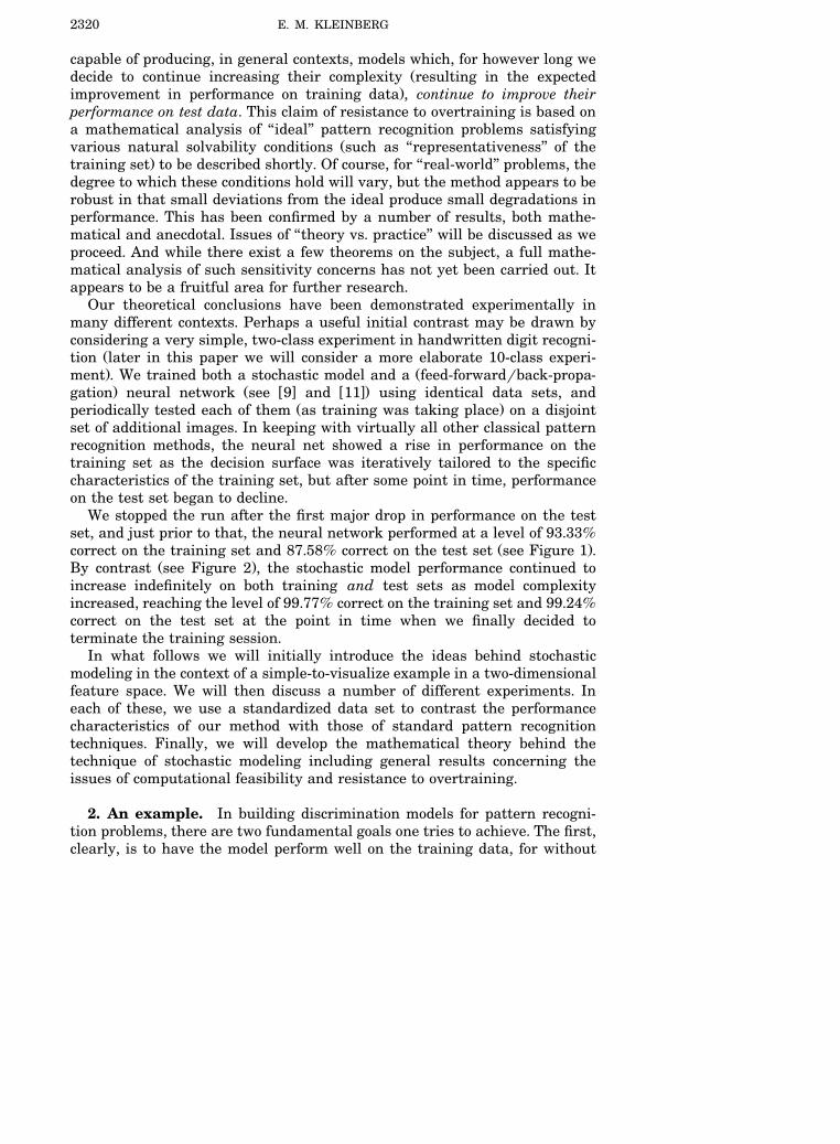
Our theoretical conclusions have been demonstrated experimentally inmany different contexts. Perhaps a useful initial contrast may be drawn byconsidering a very simple, two-class experiment in handwritten digit recogni-

Žtion later in this paper we will consider a more elaborate 10-class experi-. Žment . We trained both a stochastic model and a feed-forwardrback-propa-. Ž w x w x.gation neural network see 9 and 11 using identical data sets, and

Ž .periodically tested each of them as training was taking place on a disjointset of additional images. In keeping with virtually all other classical patternrecognition methods, the neural net showed a rise in performance on thetraining set as the decision surface was iteratively tailored to the specificcharacteristics of the training set, but after some point in time, performanceon the test set began to decline.

We stopped the run after the first major drop in performance on the testset, and just prior to that, the neural network performed at a level of 93.33%

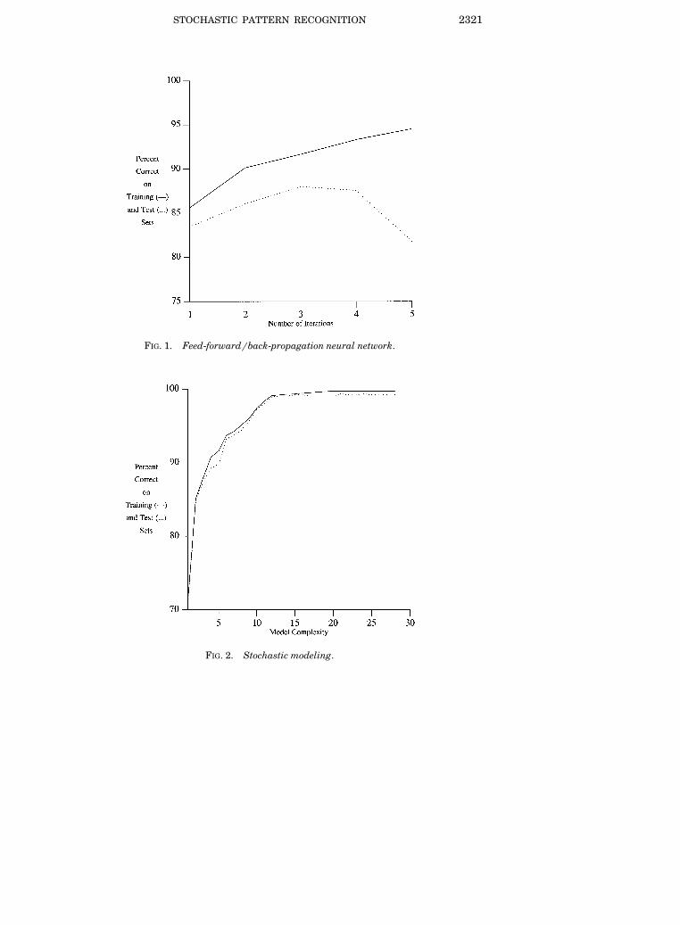
Ž .correct on the training set and 87.58% correct on the test set see Figure 1 .Ž .By contrast see Figure 2 , the stochastic model performance continued to

increase indefinitely on both training and test sets as model complexityincreased, reaching the level of 99.77% correct on the training set and 99.24%correct on the test set at the point in time when we finally decided toterminate the training session.

In what follows we will initially introduce the ideas behind stochasticmodeling in the context of a simple-to-visualize example in a two-dimensionalfeature space. We will then discuss a number of different experiments. Ineach of these, we use a standardized data set to contrast the performancecharacteristics of our method with those of standard pattern recognitiontechniques. Finally, we will develop the mathematical theory behind thetechnique of stochastic modeling including general results concerning theissues of computational feasibility and resistance to overtraining.

2. An example. In building discrimination models for pattern recogni-tion problems, there are two fundamental goals one tries to achieve. The first,clearly, is to have the model perform well on the training data, for without

STOCHASTIC PATTERN RECOGNITION 2321

FIG. 1. Feed-forwardrback-propagation neural network.

FIG. 2. Stochastic modeling.

E. M. KLEINBERG2322

this, there is no chance of decent performance in the real world. The second isto construct the model in such a way that its performance on training data‘‘projects’’ to comparable performance in the real world. Of course, the ‘‘realworld’’ in this context is usually some set of test data on which the completedmodel can be evaluated. One might simply define the ‘‘projectability’’ of amodel to be 1 minus the difference in performance between training and test

Žsets so that the larger the projectability rating, the more projectable the.model .

As we discussed above, these two goals are traditionally viewed as mutu-ally conflicting. In common practice, it is usually the case that very simplemodels perform poorly on training data but have high projectability, whilecomplex models perform well on training data but have low projectability.

The underlying idea behind our approach is this: given a problem, we willinitially, in some routine, mechanical way, generate many very simple,so-called ‘‘weak models’’ for the problem which, although probably extremelyinaccurate on the training set, will all be highly projectable. We will thentake these weak models and combine them in a certain way to form a new,so-called ‘‘stochastic model.’’ The key point is that the method of combiningthem will have the property that the projectability of the combined, stochasticmodel will be comparable to that of the component weak models from which itis built, yet, if enough weak models are used, the performance on the trainingset of the combined, stochastic model can be made arbitrarily good.

Before developing the formal theory associated with our approach, let uswork through a simple example.

Let us assume that we are interested in a particular three-class patternrecognition problem, and that we are far enough along in the process so as tohave settled on a mode of feature extraction whereby the objects amongwhich we are trying to distinguish have been reduced to points sitting in a

Ž w xbounded region of some Euclidean space, the so-called feature space see 5w x.and 15 . For example, the classes might be those associated with handwrit-

ten images of 1’s, 2’s and 3’s, and the feature extraction process might extract256 numeric features per image using a simple 16 = 16 gray-scale digitiza-tion. In this case, each such handwritten image would be reduced to a pointsitting in Euclidean 256-space.

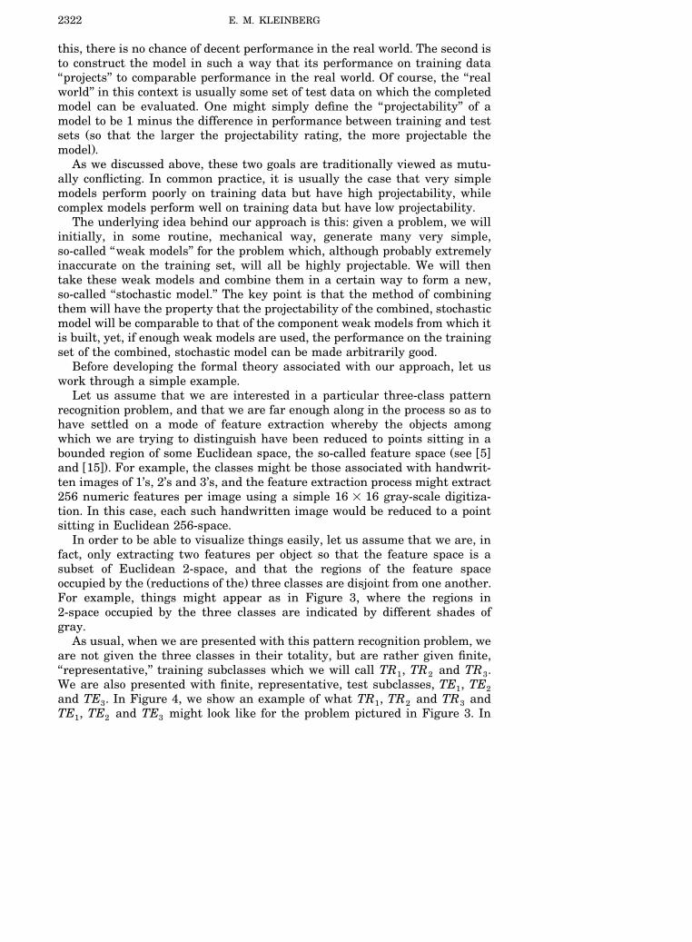
In order to be able to visualize things easily, let us assume that we are, infact, only extracting two features per object so that the feature space is asubset of Euclidean 2-space, and that the regions of the feature space

Ž .occupied by the reductions of the three classes are disjoint from one another.For example, things might appear as in Figure 3, where the regions in2-space occupied by the three classes are indicated by different shades ofgray.

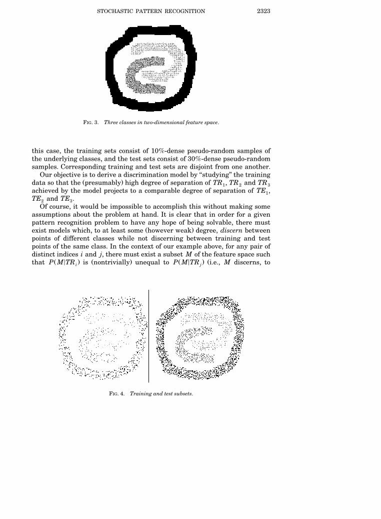
As usual, when we are presented with this pattern recognition problem, weare not given the three classes in their totality, but are rather given finite,‘‘representative,’’ training subclasses which we will call TR , TR and TR .1 2 3We are also presented with finite, representative, test subclasses, TE , TE1 2and TE . In Figure 4, we show an example of what TR , TR and TR and3 1 2 3TE , TE and TE might look like for the problem pictured in Figure 3. In1 2 3


FIG. 3. Three classes in two-dimensional feature space.

this case, the training sets consist of 10%-dense pseudo-random samples ofthe underlying classes, and the test sets consist of 30%-dense pseudo-randomsamples. Corresponding training and test sets are disjoint from one another.

Our objective is to derive a discrimination model by ‘‘studying’’ the trainingŽ .data so that the presumably high degree of separation of TR , TR and TR1 2 3

achieved by the model projects to a comparable degree of separation of TE ,1TE and TE .2 3

Of course, it would be impossible to accomplish this without making someassumptions about the problem at hand. It is clear that in order for a givenpattern recognition problem to have any hope of being solvable, there must

Ž .exist models which, to at least some however weak degree, discern betweenpoints of different classes while not discerning between training and testpoints of the same class. In the context of our example above, for any pair ofdistinct indices i and j, there must exist a subset M of the feature space such

Ž < . Ž . Ž < . Žthat P M TR is nontrivially unequal to P M TR i.e., M discerns, toi j

FIG. 4. Training and test subsets.

E. M. KLEINBERG2324

.some extent, training set i from training set j , yet, for each index k,Ž < . Ž . Ž < . ŽP M TR is approximately equal to P M TE i.e., corresponding trainingk k

.and test sets are indiscernible by M .Upon reflection, it turns out that our formalization of discernibility has a

simple flaw, because it really only implies that TR and TR have some locali jdiscernibility from one another over that region of the feature space occupiedby M; if this region is relatively small, then TR and TR might still bei jessentially indiscernible. Thus, in order to have the desired discernibilitybetween TR and TR , we require the existence of a collection of sets Mi jwhich is spread over the feature space such that for every M in the collection,Ž < . Ž < .P M TR / P M TR . We will leave the precise definition of the concepti j

‘‘spread over the feature space’’ for Section 4 of this paper, but informally,the sets in such a spread collection should treat training points of any givenclass equally so far as their degree of coverage by sets in the collection isconcerned.

In practice, since representative training and test sets are usually as-sumed to be spatially distributed throughout the region of the feature space

Žoccupied by the underlying class which is clearly the case for the example at.hand , the requirement of indiscernibility between training and test sets

with respect to a set M usually results, routinely, if we simply require thatM be, in some sense, topologically ‘‘thick,’’ that is, that it not consist of smallregions of the feature space which might capture individual points from atraining set without simultaneously capturing nearby points from the corre-sponding test set.

For the example under consideration, we used large rectangular regions,with area close to 50% that of the full feature space, as our thick subsets. Inparticular, for i / j, let Q denote the collection of those large rectangles,i, j

Ž < . Ž < .M, in the feature space such that P M TR / P M TR . Then, for eachi jŽ .i / j, Q is approximately a spread collection of sets having the desiredi, j

discernibility and indiscernibility properties. We will refer to regions in theunion of the Q as weak models for the problem at hand.i, j

Let us now use these weak models to actually construct a ‘‘stochasticdiscrimination model.’’ We will proceed somewhat informally here}the readerwho, at this time, desires more formal detail, or actual proof, should refer toSection 4.

Our model will be built by carrying out random sampling from the collec-tions Q . In fact, for any point q in our feature space and any i / j,i, j1 F i, j F 3, we define a random variable X q on Q byŽ i, j. i, j

<x q y P M TRŽ . Ž .M jqX M s 2 y 1,Ž .Ž i , j. < <ž /P M TR y P M TRŽ . Ž .i j

where x denotes the characteristic function of M. Given the nature of Q ,M i, jit is not very difficult to prove that the expectation of X q is 1 if q is aŽ i, j.member of TR , is y1 if q is a member of TR and is something close to 0 ifi jq is in TR , k / i, k / j.k


If we now define, for any point q in our feature space and any i, 1 F i F 3,1q q qthe random variable k to be Ý X , then the expectation of k will be 1i j/ i Ž i, j. i2

if q is a member of TR , and less than 0 otherwise.iConsider now the following ‘‘first pass’’ at a stochastic discrimination

model for our problem: given a point q in the feature space, in order toclassify q simply evaluate each of k q, k q and k q at a randomly chosen point1 2 3in each of their respective sample spaces; now classify q as being of class iwhere it is the value of k q which is the largest of the three values soicalculated. Our rationale here is simply that if q were indeed of class i, thenthe expectation of k q is 1, yet the expectation of k q for j different from i isi jless than 0.

ŽIf instead of sampling only once, we do it many times and take the.average of the values computed , then, by the law of large numbers, the

Ž .variance of the ‘‘average’’ variable goes to 0, and so the probability of beingclose to the expectation goes to 1. Thus, under our assumption that theclasses Q are spread and have appropriate discernibility properties, thei, jaccuracy of such discrimination models on the training set goes to 100%.

Furthermore, because of our indiscernibility assumption concerning theŽ . qQ , the expectations and the variances of the k are approximately thei, j j

same whether q is a training point or a test point. As a result, our discussionconcerning the accuracy of our stochastic discrimination model on the train-ing set applies to the test set as well. And so, as the size of our randomsample from the Q increases, the accuracy of the stochastic model on bothi, jthe training and the test sets goes to 100%.

Let us make a remark concerning the rate of convergence. Given thedefinition of X q , it is clear that its variance can be driven up by smallŽ i, j.

< Ž < . Ž < . < Ž .values of P M TR y P M TR . If we define the i, j -enrichment degree ofi ja collection Q of weak models to be

< <inf P M TR y P M TR M g Q ,Ž . Ž .½ 5i j

then one can derive an estimate of the number of weak models needed inorder that the stochastic model built from them achieves a given level of

Ž . Ž .performance as a function of a that level of performance and b theenrichment degree of the set from which the weak models were selected. Asimple analysis of this will be carried out in Section 4, but we might note herethat for a two-class, i vs. j, pattern recognition problem, the size of the weakmodel sample needed so that the expected accuracy of the associated stochas-tic model is greater than 1 y 1ru is directly proportional to u and inversely

Ž .proportional to the square of the i, j -enrichment degree.Given this fact, one might be tempted to work exclusively with highly

enriched collections of weak models. However, it is clearly more difficult tofind such ‘‘stronger’’ weak models, so there is an immediate time trade-offinvolved. In addition, if weak models are allowed to become too strong, theymay start to exhibit signs of overtraining leading to unacceptable degradationof our indiscernibility conditions.

E. M. KLEINBERG2326

Before considering the application of our method to the synthetic problemillustrated above, let us make several general comments in order to providesome historical perspective on this approach. The underlying ideas behindstochastic discrimination, the basis for our work here, were first introduced inw x16 . Immediately following this initial work, we began experimenting withimplementations of the method, and, simultaneously, began formulating themathematical concepts needed to analyze this practical application ofstochastic discrimination to statistical pattern recognition problems. Earlydrafts of the current paper, including the mathematical conditions needed toguarantee perfect solvability of problems derived from representative train-ing sets, have been in circulation since 1991. Based on these drafts, othersbegan research on our methods and on variations of our implementation. Forexample, one such variant, based on ideas by Ho for changing the random

Žw x. w xvariable X 13 , was developed and studied extensively by Berlind 2 .Ž i, j.w xAnd in 14 , Ho studied the use of leaves from fully split decision trees, where

each leaf was perfectly enriched for one class, and each point was covered byexactly one leaf of each tree. An objective here was the desire for good‘‘spread’’ in the collection of weak models.

The general notion of improving classifier accuracy by combining a numberof less accurate classifiers trained for the same task has been around for

Ž w x w x. Žquite some time see 10 and 12 . Even in the context of PAC learning see,w x w x w x.e.g., 6 , 8 and 20 , there has been recent work concerned with ‘‘boosting’’

accuracy by using, in concert, numbers of different ‘‘weak’’ hypotheses. Theweak hypotheses here are generated sequentially by training on differentsets of examples, where the derivation of each such set of examples at a given

Ž .stage is based on what took place at previous stages. The relatively smallnumber of weak hypotheses generated in this way are then combined usingmajority vote. In practice, it has helped to improve performance of variousclassification approaches, as one would expect from any of the combinationmethods.

Our approach is fundamentally different in that it is based on randomsampling from the space of all possible classifiers, that is, sampling from thepower set of the feature space. And while accuracy increases with the use oflarger and larger samples of such subsets, this is in no way a serial learningtechnique because the sampling can be carried out entirely in parallel. Thus,on a suitable machine, one of our stochastic models can be built basically inone step. In practice, we restrict our attention to subspaces satisfying certain

Žrequired conditions based on the notions of spread, indiscernibility and.enrichment , and even here, the samplingrcombining process maintains

Ž .projectability independent of the number of weak models samples chosen,and hence, of the resulting complexity of the classifier. In effect, our notion ofstochastic modeling is a technique, based on the laws of large numbers andthe central limit theorem, to amplify small differences through the use ofdiscrete stochastic processes.

As mentioned above, stochastic models are computationally feasible both toproduce and to use. They are especially suitable to parallel implementation,


for both the generation and evaluation of component weak models are thingsŽbest carried out in parallel. Indeed, the weak models can all be chosen if

. Žbuilding the stochastic model or evaluated at a point in the feature space if.evaluating the stochastic model at a point in the feature space simultane-

ously. Some parallel implementations have, in fact, been tested experimen-tally. This work will be reported on elsewhere.

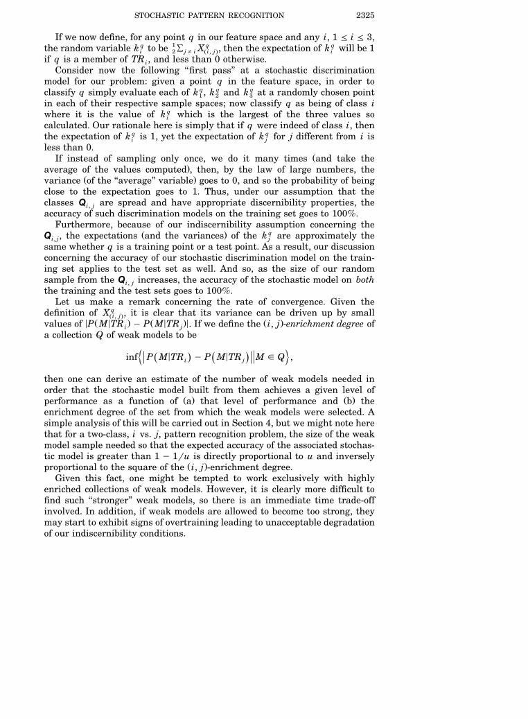
Let us now take a look at our attempt to build a stochastic model for theproblem illustrated in Figures 3 and 4 above. Just as described, we carried

Ž .out random sampling from the collection of large rectangular weak models.During the course of our sampling, we periodically evaluated stochasticmodels based on the samples of weak models we had to that point in time.For example, with a total sample size of only two weak models, the associatedstochastic model performed at a level of 44.63% on the training set and43.94% on the test set. In Figure 5, we tabulate stochastic model performanceas a function of sample size for a range of values during our run.

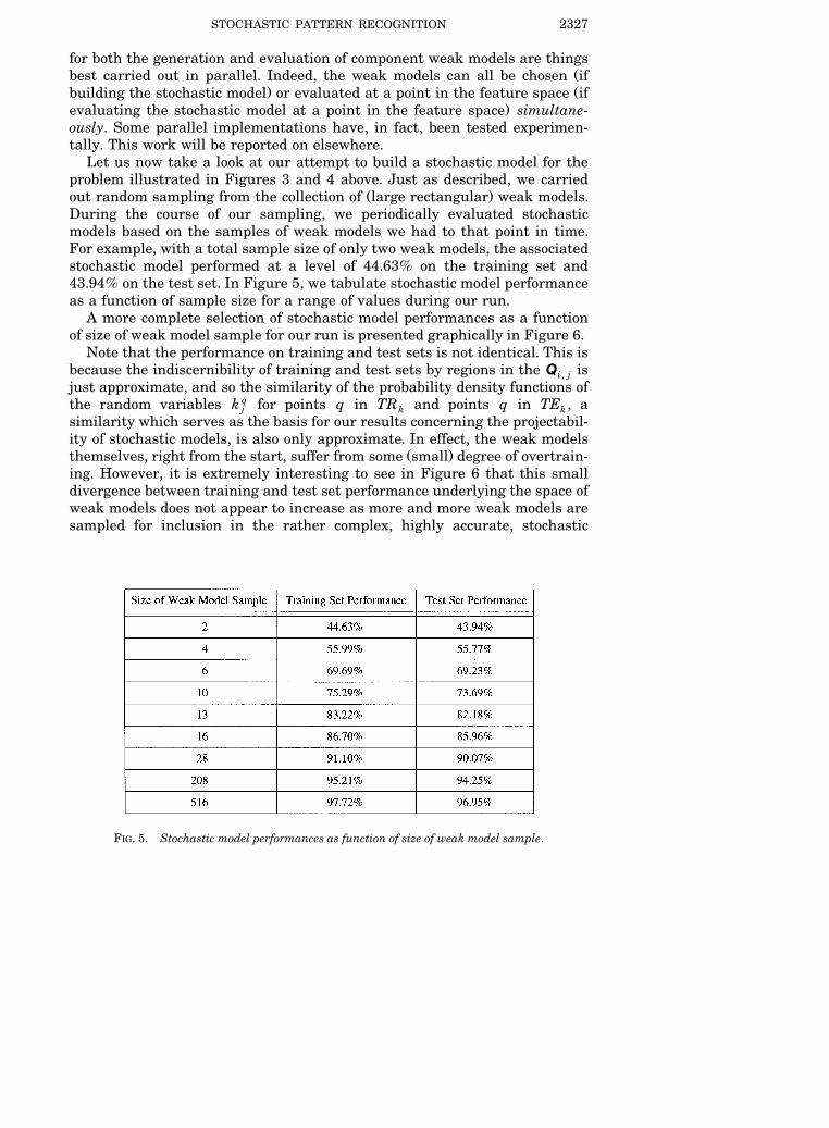
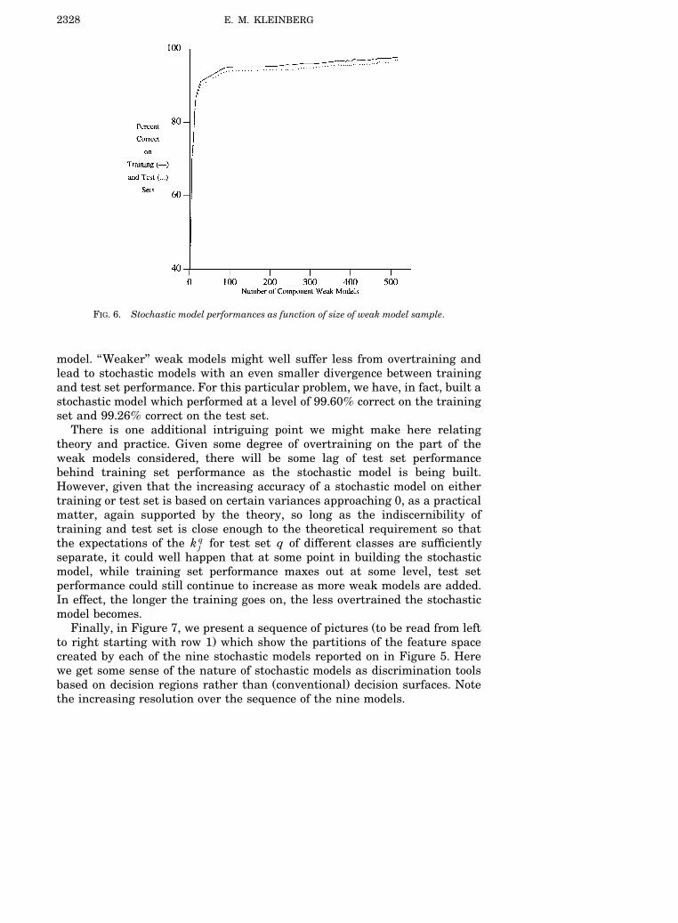
A more complete selection of stochastic model performances as a functionof size of weak model sample for our run is presented graphically in Figure 6.

Note that the performance on training and test sets is not identical. This isbecause the indiscernibility of training and test sets by regions in the Q isi, jjust approximate, and so the similarity of the probability density functions ofthe random variables k q for points q in TR and points q in TE , aj k ksimilarity which serves as the basis for our results concerning the projectabil-ity of stochastic models, is also only approximate. In effect, the weak models

Ž .themselves, right from the start, suffer from some small degree of overtrain-ing. However, it is extremely interesting to see in Figure 6 that this smalldivergence between training and test set performance underlying the space ofweak models does not appear to increase as more and more weak models aresampled for inclusion in the rather complex, highly accurate, stochastic

FIG. 5. Stochastic model performances as function of size of weak model sample.

E. M. KLEINBERG2328


model. ‘‘Weaker’’ weak models might well suffer less from overtraining andlead to stochastic models with an even smaller divergence between trainingand test set performance. For this particular problem, we have, in fact, built astochastic model which performed at a level of 99.60% correct on the trainingset and 99.26% correct on the test set.

There is one additional intriguing point we might make here relatingtheory and practice. Given some degree of overtraining on the part of theweak models considered, there will be some lag of test set performancebehind training set performance as the stochastic model is being built.However, given that the increasing accuracy of a stochastic model on eithertraining or test set is based on certain variances approaching 0, as a practicalmatter, again supported by the theory, so long as the indiscernibility oftraining and test set is close enough to the theoretical requirement so thatthe expectations of the k q for test set q of different classes are sufficientlyjseparate, it could well happen that at some point in building the stochasticmodel, while training set performance maxes out at some level, test setperformance could still continue to increase as more weak models are added.In effect, the longer the training goes on, the less overtrained the stochasticmodel becomes.

ŽFinally, in Figure 7, we present a sequence of pictures to be read from left.to right starting with row 1 which show the partitions of the feature space

created by each of the nine stochastic models reported on in Figure 5. Herewe get some sense of the nature of stochastic models as discrimination tools

Ž .based on decision regions rather than conventional decision surfaces. Notethe increasing resolution over the sequence of the nine models.


FIG. 7. Stochastic partitions of feature space.

3. Some experimental results. Let us now consider experimental re-sults in handwritten digit recognition. The algorithmic implementation of ourmethod which was used here was identical to that developed above for use inthe two-dimensional feature space example. The only adjustment needed wasa simple modification dictated by the fact that our underlying feature spacewas no longer two dimensional.

Our study was carried out on handwritten digits comprising a standarddatabase supplied by the National Institute of Standards and TechnologyŽ .N.I.S.T. containing writing samples from thousands of different people. Weselected sample images from the set by taking, for the first 1000 differentpeople represented, the first example of each digit written by each of them. Inthis way, we were able to put together a set of almost 10,000 digits containingapproximately 1000 examples of each digit.

E. M. KLEINBERG2330

The handwritten digits contained in this database were originally scannedand binarized at 300 dpi, but we preprocessed them prior to sending them tothe stochastic modeling routine. The preprocessing reduced each scannedimage to a fixed-length numeric record by first size-normalizing the image to16 = 16, and then, within each of the 256 windows in the image associatedwith this size normalization, calculating the number of black pixels presentas a fraction of the total number of pixels in the window. We then thresholdedthe fraction against 0.2 to decide whether to call the window ‘‘on’’ or ‘‘off.’’ Inother words, if the fraction of black pixels in the window was greater than0.2, we assigned the field value 1 to that window for the record associatedwith the given image}otherwise we assigned the field value 0. In this way,each original scan was reduced to a fixed-length numeric record of 256integer fields, each of whose values was either 0 or 1.

Once the image database was reduced in this way, we selected the first4997 records as our training set and reserved the remaining 4975 records asour test set. In this way, we had about 500 examples of each digit type ineach of the training and test sets. Given the way in which we selected ourimages at the start, this guaranteed that not only were the training and testsets disjoint from one another, but also that no person with a handwrittenimage appearing in the training set contributed any images to the test set.

We then fed the training set of records into our stochastic model buildingŽ .program and began the weak model sampling process. One should keep in

mind that since our feature space was now a subset of Euclidean 256-space,our weak models were now constructed from large, 256-dimensional rectan-

� 4256gular parallelopipeds, that is, large regions in the feature space 0, 1which can be written in the form

x , x , . . . , x for each i , a F x F b ,� 4Ž .1 2 256 i i i

Ž . Ž . � 4256where a , a , . . . , a and b , b , . . . , b are members of 0, 1 . Given1 2 256 1 2 256the small size of the training set, we actually set things up so that the onlysuch regions considered as candidates were those which contained at leastone member of the training set.

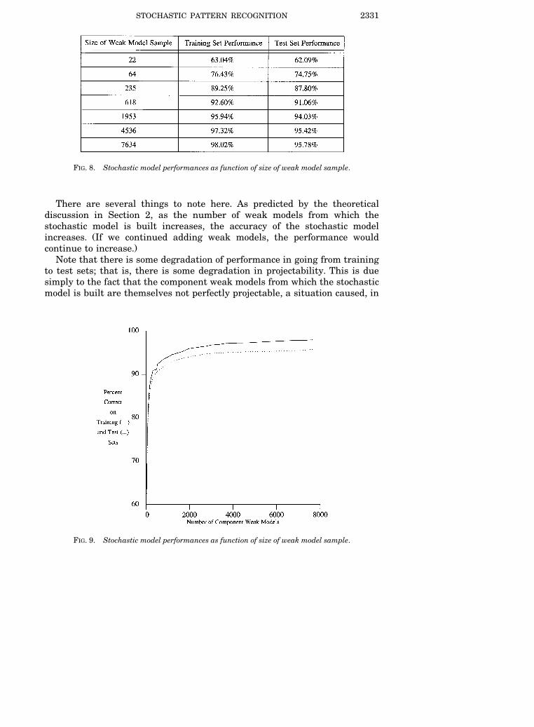
Every so often during the run, as the sample of weak models was accumu-lating, we evaluated the performance of the stochastic model based on thesample as it existed at that point in time. For example, we first evaluatedperformance when our random sample consisted of 22 weak models. At thatpoint in time, the stochastic model performed at a 63.04% level of accuracy onthe training set and a 62.09% level of accuracy on the test set. The nextevaluation took place when the sample size was 64, and here the stochasticmodel performed at a 76.43% level of accuracy on the training set and a74.75% level of accuracy on the test set.

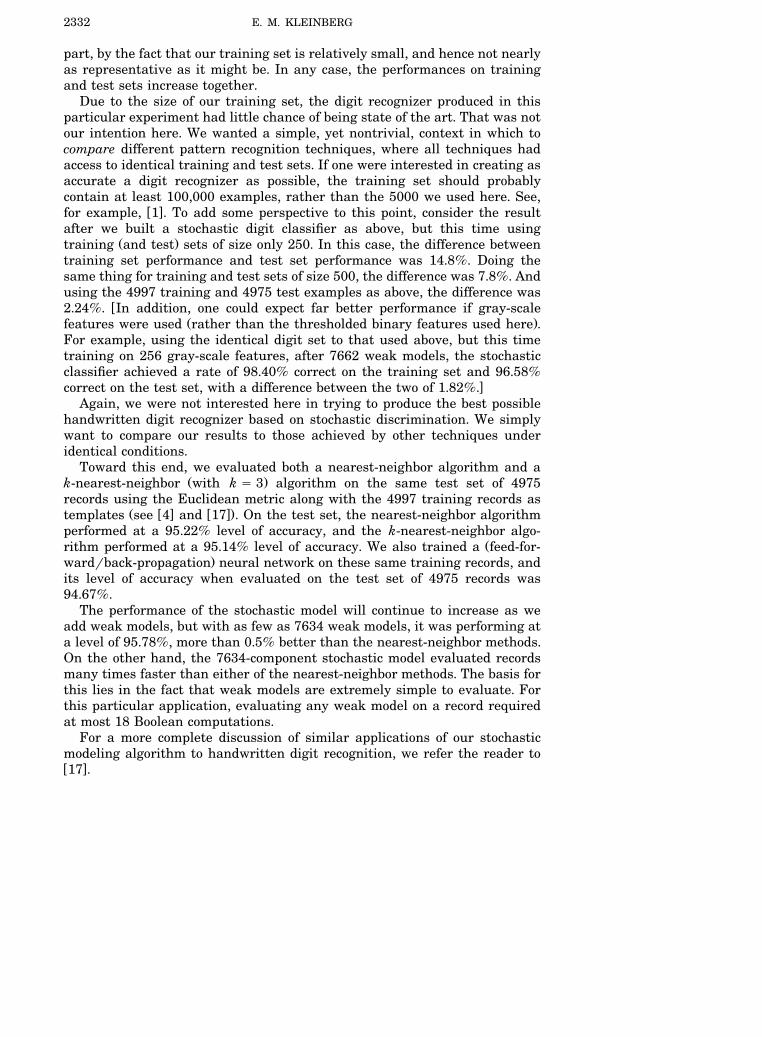
During the course of the run, many such evaluations took place. In Figure8, we tabulate a short selection of them, and in Figure 9, we graph bothtraining set performance and test set performance as functions of samplesize.



There are several things to note here. As predicted by the theoreticaldiscussion in Section 2, as the number of weak models from which thestochastic model is built increases, the accuracy of the stochastic model

Žincreases. If we continued adding weak models, the performance would.continue to increase.

Note that there is some degradation of performance in going from trainingto test sets; that is, there is some degradation in projectability. This is duesimply to the fact that the component weak models from which the stochasticmodel is built are themselves not perfectly projectable, a situation caused, in


E. M. KLEINBERG2332

part, by the fact that our training set is relatively small, and hence not nearlyas representative as it might be. In any case, the performances on trainingand test sets increase together.

Due to the size of our training set, the digit recognizer produced in thisparticular experiment had little chance of being state of the art. That was notour intention here. We wanted a simple, yet nontrivial, context in which tocompare different pattern recognition techniques, where all techniques hadaccess to identical training and test sets. If one were interested in creating asaccurate a digit recognizer as possible, the training set should probablycontain at least 100,000 examples, rather than the 5000 we used here. See,

w xfor example, 1 . To add some perspective to this point, consider the resultafter we built a stochastic digit classifier as above, but this time using

Ž .training and test sets of size only 250. In this case, the difference betweentraining set performance and test set performance was 14.8%. Doing thesame thing for training and test sets of size 500, the difference was 7.8%. Andusing the 4997 training and 4975 test examples as above, the difference was

w2.24%. In addition, one could expect far better performance if gray-scaleŽ .features were used rather than the thresholded binary features used here .

For example, using the identical digit set to that used above, but this timetraining on 256 gray-scale features, after 7662 weak models, the stochasticclassifier achieved a rate of 98.40% correct on the training set and 96.58%

xcorrect on the test set, with a difference between the two of 1.82%.Again, we were not interested here in trying to produce the best possible

handwritten digit recognizer based on stochastic discrimination. We simplywant to compare our results to those achieved by other techniques underidentical conditions.

Toward this end, we evaluated both a nearest-neighbor algorithm and aŽ .k-nearest-neighbor with k s 3 algorithm on the same test set of 4975

records using the Euclidean metric along with the 4997 training records asŽ w x w x.templates see 4 and 17 . On the test set, the nearest-neighbor algorithm

performed at a 95.22% level of accuracy, and the k-nearest-neighbor algo-Žrithm performed at a 95.14% level of accuracy. We also trained a feed-for-

.wardrback-propagation neural network on these same training records, andits level of accuracy when evaluated on the test set of 4975 records was94.67%.

The performance of the stochastic model will continue to increase as weadd weak models, but with as few as 7634 weak models, it was performing ata level of 95.78%, more than 0.5% better than the nearest-neighbor methods.On the other hand, the 7634-component stochastic model evaluated recordsmany times faster than either of the nearest-neighbor methods. The basis forthis lies in the fact that weak models are extremely simple to evaluate. Forthis particular application, evaluating any weak model on a record requiredat most 18 Boolean computations.

For a more complete discussion of similar applications of our stochasticmodeling algorithm to handwritten digit recognition, we refer the reader tow x17 .


There are many other experiments which have been carried out in order tofurther evaluate, anecdotally, the degree to which theory and practice differwhen our mathematical assumptions are not strictly met. Let us briefly

w xmention two of them. In 18 , we considered a synthetic problem involvingtwo overlapping classes in Euclidean 2-space. The classes were produced by

Ž . Ž .simply taking Gaussian joint distributions centered at 80, 80 for class 0Ž . Ž .and 120, 120 for class 1 . In each case, x and y varied independently, with

Ža standard deviation of 20. For this problem, the Bayes error rate estimated.by numerical integration was 0.07866, implying a maximum correct rate of

92.13%. Pseudo-random training and test sets, each of size 2000, wereconstructed, and we proceeded to build a stochastic model by sampling thesame space of weak models, based on large rectangular regions, used above.Despite the overlap of the classes, as the number of contributed weak modelsincreased, performance of the stochastic model on both training and test sets

Ž .increased. The Bayes maximum correct rate was reached after fewer than150 weak models were chosen.

Žw x.In another experiment based on data provided by Project Statlog 19 , theobject was to classify boundary types in DNA sequences. Feature vectors werederived from contiguous blocks within sequences, and each consisted of 180binary fields. This was a problem formally defined in terms of specific

Ž .training and test sets of sizes 2000 and 1186, respectively , and over time,many of the different pattern recognition techniques were tried out on it inorder to evaluate their relative levels of performance. The resulting accura-

w xcies of more than 20 different methods are reported in 19 . These extremelyinteresting results show, for example, test set performances of KNN at

Ž .85.4%, BackProp at 91.2% and Cart at 91.5%. The best result Polarreported 95.9%. We built a stochastic model for this problem involving6451-many weak models sampled from exactly the same sort of space, basedon large rectangular parallelopipeds, used above, and its test set performancewas 96.2%.

ŽIt is important to note that for this and every other experimental result.reported here , the same stochastic model building program was used. The

only user-supplied information which varied from run to run was the data inthe training and test sets.

w xSee 18 for algorithmic detail on a practical implementation of stochasticdiscrimination, and for the application of that implementation to these andother problems.

4. Mathematical considerations. In this section we will develop themathematics underlying the ideas introduced in Section 2. Our first goal is to

Žformalize the notion of a collection of subsets of the feature space usually, a.collection of weak models being ‘‘spread.’’ This was a key concept involved

with our initial discussion of indiscernibilityrdiscernibility as applied to thevarious training and test sets, and it was never really pinned down at thattime.

E. M. KLEINBERG2334

As before, we assume that our underlying feature space, F, is finite. Wewill use the counting measure m on F and the counting measure n on thepower set of F, F, to calculate probabilities whenever necessary.

NOTATION. We denote by r the function from F = F into the reals givenby

m S l TŽ .for each pair of subsets S, T of F , T / B, r S, T s .Ž . Ž .

m TŽ .Ž . Ž < .Viewing F as a sample space, r S, T is just P S T , that is, the probability

of S given T. This function r will be an extremely useful notational devicefor us.

NOTATION. Given a real number x, a member A of F and a subset M of F,Ž .let M denote the set of those M in M such that r M, A s x.x, A

Ž .Intuitively, for any two subsets S and T of F, r S, T equals the fractionalamount of T which is captured by S. Thus, we might make the followingtrivial observation: given any real number x, member A of F, subset M of Fand members M and N of M , the probability that M captures a point inx, AA is equal to the probability that N captures a point in A, that is,

< <P p g M p g A s P p g N p g A .Ž . Ž .F F

ŽSince we will be dealing with several different probability spaces in whatfollows, there might be times when confusion could arise as to just whichspace we are taking probabilities with respect to. At times of such potentialambiguity, we will use P to denote probabilities taken with respect to theT

.space T.The notion of ‘‘spread’’ derives from what might be viewed as the ‘‘dual’’ of

this trivial observation.

DEFINITION. Let M be a collection of subsets of a given feature space F,and let A be a subset of F. Then M is said to be A-uniform if, for any realnumber x such that M is nonempty, given any two points p and q in A,x, Athe probability relative to the space F that p is captured by a member of Mx, Ais equal to the probability that q is captured by a member of M , that is,x, A

< <P p g M M g M s P q g M M g M .Ž . Ž .F x , A F x , A

An A-uniform collection of subsets of F is, in some intuitive sense, ‘‘spreadover A.’’

While it is easy to construct examples of collections of subsets of F whichare not A-uniform, it is also the case that examples of such uniformity occurquite naturally. In fact, given any subset A of F, a simple counting argumentshows that, for any real number x such that F is nonempty, the probabil-x, Aity relative to the space F that a member of A is captured by a member ofF is x. Thus, the full power set of F is always A-uniform for every subsetx, AA of F.


Ž < .It turns out that P q g M M g M s x holds for any collection ofF x, Asubsets M which is A-uniform.

LEMMA 1. Let F be a given feature space, and let A be a subset of F.Suppose M is an A-uniform collection of subsets of F. Then, for any realnumber x such that M is nonempty,x, A

<P q g M M g M s xŽ .F x , A

for every q in A.

PROOF. Since M is A-uniform, we know that, for some real y,

<P q g M M g M s yŽ .F x , A

Ž .for every q in A. Let a denote the common number of elements in M l AŽ .for any M in M , let b denote the number of elements in A, let c denotex, AŽ . Ž . Ž .the common number of sets M in M such that any given q in A is ax, A

member of M, and let d denote the number of elements of M . We canx, AŽ .count the number of ordered pairs q, M such that q g M l A and M g Mx, A

in either of two ways, getting bc one way and ad the other. Thus, arb s crd,and since we chose a, b, c and d such that arb s x and crd s y, we haveshown that x s y. I

In light of this result, we are now in a position to formally define the notionof ‘‘spread’’ needed for our work. In considering the following notation anddefinition, it would be helpful for the reader to picture an m-class patternrecognition problem in the feature space F, where, for each i, C is theitraining set associated with class i.

² :NOTATION. Given a positive integer m, a sequence C s C , C , . . . , C1 2 m² :of subsets of F and a sequence x s x , x , . . . , x of reals, M denotes1 2 m x , C

Ž .the set of those M in M such that, for each j, 1 F j F m, r M, C s x .j j

² :DEFINITION. For a given sequence of subsets C s C , C , . . . , C of F, a1 2 msubset M of F is said to be C-uniform if, for every j, 1 F j F m, every

² :member q of C and every sequence x s x , x , . . . , x of real numbersj 1 2 msuch that M is nonempty,x , C

<P q g M M g M s x .Ž .F x , C j

Given an m-class pattern recognition problem in F with training setsŽ .TR s TR , TR , . . . , TR , any TR-uniform collection of subsets of F is1 2 m

‘‘sufficiently spread over the training sets’’ for our development to succeed.Let us make a comment here concerning the formal definition of uniform-

ity given above. Throughout this paper we will give a number of definitionsinvolving strict equalities such as, for example, the equality

<P q g M M g M s xŽ .F x , C j

E. M. KLEINBERG2336

given above. In actual practice, however, such equalities might only besatisfied to within some small real value « . Depending on just how far off weare in any given instance, there may be some commensurate drop in variousother factors predicted by our theory. However, small errors in satisfyingequalities in definitions result in small errors in predicted outcome. In thissection our goal is to present the underlying theory of stochastic modeling assimply as possible, without the additional complication of estimating deriva-

w xtive error. For a rigorous treatment of these issues, we refer the reader to 2w xand 3 .

We now attack the issue of indiscernibility between corresponding trainingand test sets. As already discussed in Section 2, this concept is dependent notonly on the training and test sets themselves, but also on a class of subsets of

Ž .the feature space such as a class of thick regions . As discussed previously, inorder for two given subsets A and B of F to be indiscernible with respect to a

Ž .collection M of subsets of F, we would certainly require that r M, A beŽ . Ž .approximately equal to r M, B for every member M of M. However, inlight of our recently completed discussion concerning uniformity, it seemsreasonable that if A were truly indiscernible from B with respect to sets inthe collection M, then if M were ‘‘spread’’ over A, M would also have to be‘‘spread’’ over B. On the other hand, the notion of indiscernibility existsindependently of any uniformity which may or may not hold for the setsinvolved, so our definition must consider concepts related to the degree ofspread of sets in M over the regions A and B. Formalizing this to our currentcontext of training and test subsets of an m-class pattern recognition prob-lem, we introduce the following definitions which, as before, will be easier toconsider if the reader pictures an m-class pattern recognition problem in thefeature space F, where, for each i, C is the training set associated with classii and D is the test set associated with class i.i

DEFINITION. Given any subset M of F, any positive integer m, any² :sequence C s C , C , . . . , C of subsets of F and any sequence x s1 2 m

² :x , x , . . . , x of reals such that M is nonempty, for any j, 1 F j F m,1 2 m x , Cf j is the random variable defined on C whose value at any q is given byM , x , C j

j <f q s P q g M M g M .Ž . Ž .M , x , C F x , C

In some sense, the random variables f j provide ‘‘profiles of coverage’’M , x , Cof the sets in C by members of M. We are thus led naturally to the followingdefinition.

DEFINITION. Given any subset M of F, any positive integer m and any two² : ² :sequences C s C , C , . . . , C and D s D , D , . . . , D of subsets of F,1 2 m 1 2 m

we say that C is M-indiscernible from D if:

Ž . Ž . Ž .a for any j, 1 F j F m, and any M in M, r M, C s r M, D ;j jŽ . ² :b for any sequence x s x , x , . . . , x of reals and for any j, 1 F j F m,1 2 m

the random variables f j and f j have the same probability densityM , x , C M , x , Dfunctions.


It is immediate that the notion of M-indiscernibility is an equivalencerelation. Furthermore, M-indiscernibility preserves uniformity, as shown bythe following result.

² :LEMMA 2. Given any two sequences C s C , C , . . . , C and D s1 2 m² :D , D , . . . , D of subsets of F, if C is M-indiscernible from D and M is1 2 mC-uniform, then M is D-uniform.

PROOF. We simply note that for any sequence of subsets B s² :B , B , . . . , B of F, M is B-uniform iff for every sequence x s1 2 m² :x , x , . . . , x of real numbers such that M is nonempty, for every j,1 2 m x , B1 F j F m, the pdf of the random variable f j is the function which is 1 atM , x , Bx and 0 elsewhere. The lemma is now immediate. Ij

Let us now assume for the duration of this paper that we have been givenan m-class pattern recognition problem in a feature space F; that is, assumethat we have been given, for some positive integer m and finite feature space

² : Ž .F, an m-sequence TR s TR , TR , . . . , TR of nonempty training subsets1 2 m² : Ž .of F and an m-sequence TE s TE , TE , . . . , TE of nonempty test sub-1 2 m

sets of F.Based on our discussion in Section 2, we know that in order for this

problem to be perfectly solvable, there must exist some TR-uniform collec-tion, M, of subsets of F such that TR is M-indiscernible from TE, and suchthat the different training sets in TR are ‘‘discernible’’ with respect to sets inM. For the duration of this paper, let us assume that M is a fixed TR-uniformcollection of subsets of F such that TR is M-indiscernible from TE. In orderto formalize the concept of ‘‘discernible,’’ we give the following definition.

Ž .DEFINITION. For 1 F i F m and 1 F j F m, the i, j -enrichment degree ofŽ N .a subset N of M written e is defined to bei, j

inf r M , TR y r M , TR M g N .Ž . Ž .½ 5i j

Ž . NThe subset N is said to be i, j -enriched if e ) 0.i, j

Ž .If N is i, j -enriched for a particular i and j, then TR and TR arei j‘‘discernible’’ from one another with respect to N.

Ž .As we mentioned earlier, for each j, 1 F j F m, r M, TR measures thejdegree to which the set M captures points in TR . Thus, if M were equal tojF, this value would be 1, and if M were equal to B, this value would be 0. Fora fixed value of j, if we were to view r as a random variable defined on the

1� 4space F = TR , then it is clear that its expectation would be . For if onej 2

were to go through a process deciding, with equal probability, whether eachpoint in a given set was to be removed or not, one would be expected, whendone, to have removed half the points in the set.

E. M. KLEINBERG2338

Although it is by no means the only way to do it, one might view theŽ .process of creating an i, j -enriched, TR-uniform collection of subsets of F as

one which randomly generates subsets of F and selects those M such that1Ž . Ž .r M, TR and r M, TR sit on opposite sides of the expected value . Thisi j 2

Ž .process need have no effect on the values of r M, TR for k different from ikand j, and if m is greater than 2, it is, in fact, desirable to select M which

1Ž . Ž .not only push r M, TR and r M, TR away from , but which keep alli j 21Ž .other r M, TR close to . In some sense, such collections are ‘‘neutral’’ withk 2

respect to classes other than i and j. With this in mind, we give the followingdefinition.

Ž .DEFINITION. For 1 F i F m and 1 F j F m the i, j -neutrality degree of aŽ N .subspace N of M written n is defined to bei, j

r M , TR y r M , TRŽ . Ž .k jsup M g N , k / i , j .½ 5r M , TR y r M , TRŽ . Ž .i j

Ž . NThe subset N is said to be i, j -neutral if n - 1.i, j

The virtues of enrichment and neutrality will be made clear shortly. Forthe moment, however, let us simply note that if a given TR-uniform space ofweak models has a subspace which is either enriched or neutral, then it has aTR-uniform subspace which is, similarly, enriched or neutral. For it is clearthat any subspace of a TR-uniform space W which can be written as a unionof subspaces of the form W must also be TR-uniform.x , T R

We now formalize the random variable X introduced in Section 2.Ž i, j.

Ž .DEFINITION. For any pair of integers i, j , 1 F i F m and 1 F j F m, letŽ .X be the function defined on F = M as follows: for any pair q, S inŽ i, j.

F = M,

¡ x q y r S, TRŽ . Ž .S j2 y 1, if r S, TR / r S, TR ,Ž . Ž .i j~ ž /r S, TR y r S, TRŽ . Ž .X q , S sŽ . i jŽ i , j. ¢0, if r S, TR s r S, TR ,Ž . Ž .i j

where x denotes the characteristic function of the set S.S

Since both F and M are finite sets, we can view them, under countingmeasures, as finite measure spaces; as such, X can be viewed as a randomŽ i, j.variable defined on the sample space F = M.

ŽOften, when dealing with functions of several variables such as r or.X , we will wish to hold several of the variables fixed at constant valuesŽ i, j.

and consider the resulting expression to be a function of the remainingŽ .nonfixed variables. The following well-known lambda notation is helpful inrepresenting such functions: if f is a function of n q k variables x , x , . . . , x1 2 n


and y , y , . . . , y , and a , . . . , a are k constants, then1 2 k 1 k

l x ??? l x f x , x , . . . , x , a , a , . . . , aŽ .1 n 1 2 n 1 2 k

denotes the function of n variables which results from taking f and holdingits k variables y , y , . . . , y constant at a , . . . , a , respectively.1 2 k 1 k

We now consider the question of the expectations of the X .Ž i, j.

LEMMA 3. If A is a subset of F, N is an A-uniform subspace of M and q is aw Ž .xmember of A, then the expectations of the random variables lM x q andM

w Ž .x Ž .lM r M, A both restricted to the sample space N are identical.

Ž < Ž . .PROOF. By Lemma 1, for any real x, P q g M r M, A s x s x. Thus,Fw Ž .xthe expectation of lM x q , restricted to N , is x. Clearly, the expecta-M x, A

w Ž .xtion of lM r M, A , restricted to N , is also x. Since N can be written as ax, Afinite disjoint union of sets of the form N , the lemma is now immediate. Ix, A

Thus, if N is an A-uniform subspace of M, given any two members p andw Ž .x w Ž .xq of A, the random variables lM x p and lM x q have the sameM M

probability density functions.

LEMMA 4. Let i and j be distinct integers, 1 F i F m and 1 F j F m, andŽ .let N be a TR-uniform, i, j -enriched subspace of M. Then, for any k,

1 F k F m, as q ranges over TR , the random variables which result fromk� 4restricting X to sample spaces of the form q = N, are identically dis-Ž i, j.

tributed. Let E denote the common expectation of these random variables.kThen E s 1, E s y1 and, if k / i, j, E F 2nN y 1.i j k Ž i, j.

PROOF. If the space N is of the form T for some sequence x sx , T R² :x , x , . . . , x of real numbers, and some subspace T of M, this lemma1 2 mfollows easily from Lemma 3. However, the subspace N can clearly be writtenas a finite disjoint union of nonempty sets of the form N , and so the fullx , T Rlemma is now immediate. I

Until further notice, let us assume that we are dealing with a two-classŽ .problem m s 2 , and that there exists a subset N of F which is TR-uniform

Ž .and 1, 2 -enriched, such that TR and TE are N-indiscernible. As in Section2, N is called a space of weak models. Given our current restriction totwo-class problems, our description of a stochastic discrimination modelbased on N can be made even simpler than that presented in Section 2.Indeed, our model is now basically that which classifies a point q in F to be

Ž . w Ž .xof type 1 type 2 if the average value of lM X q, M on a sufficientlyŽ1, 2.Ž .large random sample from N is greater than or equal to 0 is less than 0 .

To make this precise, let t be a given positive integer, and let us denote byX k the random variable corresponding to X associated with the kth of tŽ1, 2. Ž1, 2.trials, that is, the random variable defined on the sample space F = N t

Ž Ž .. Ž . twhose value at any point q, S , S , . . . , S is X q, S . Let Y denote1 2 t Ž1, 2. k Ž1, 2.

E. M. KLEINBERG2340

the random variable

tkX t.Ý Ž1, 2.ž /

ks1

By the central limit theorem, as t increases, the probability density functionof Y t approaches a normal probability density function having expectationŽ1, 2.that of X and having variance 1rt that of X .Ž1, 2. Ž1, 2.

t Ž . tIn particular, if, for a given t and member s s S , S , . . . , S of N , we1 2 tdefine the discrimination model M t to be that which classifies a point q to bes

t Ž Ž ..of class 1 if the value Y q, S , S , . . . , S is greater than or equal to 0,Ž1, 2. 1 2 tt Ž Ž ..and to be of class 2 if the value Y q, S , S , . . . , S is less than 0, thenŽ1, 2. 1 2 t

the probability that M t makes an error in classifying any point in thestraining set approaches 0 as t approaches `. Furthermore, given the N-indis-cernibility of TR and TE, the probability that M t makes an error insclassifying any point in the test set also approaches 0 as t approaches `.

However, let us be careful here. The notion of ‘‘probability of error’’ in thecontext of pattern recognition almost always relates to the probability rela-tive to the space of points being classified that a given point is improperlyclassified. In the discussion above concerning stochastic models, however, thisis not what we are talking about. Any conclusions we have reached thus farconcerning the accuracy of stochastic models is relative to the space N t oft-tuples of subsets of N. In other words, what we have shown is that for any

Ž .given point q in the training or test set, if m t denotes the probability that amember st of the space N t leads to a derivative model M t which misclassi-s

Ž .fies q, then as t approaches `, m t approaches 0. Thus, while from thegeneral perspective of producing solutions to pattern recognition problems,we have described a general modeling technique which succeeds in discrimi-nating between classes, we would like to analyze our approach in such a wayas to produce more conventional estimates of model accuracy.

We begin with a couple of definitions.

DEFINITION. Given a collection N of subsets of F, a level-t stochasticmodel built from N is a model of the form M t for some member st of N t.s

For binary discrimination problems, it is standard to equate any discrimi-nation model with the set of points in the feature space which the modelclassifies as being of type 1. Given this, the following definition is reasonable.

DEFINITION. Given a binary discrimination model M and a sequence² : ŽT s T , T of subsets of F, the accuracy of M relative to separating the1 2

. w Ž .xclasses T and T denoted a M, T is given by1 2

a M , T s r M , T y r M , T .Ž . Ž . Ž .1 2


Ž . Ž .Here a M, T ranges between 1 and y1. If a M, T s 1, the classificationmodel M is perfect.

t t Ž .For the case at hand, every point s of N leads to a potentially differentŽ .t tmodel M . Thus, we are interested not so much in a M , TR for anys s

t Ž .tparticular s , but rather in the expected value of a M , TR as a function ofst. In particular, we would like some idea as to how large t must be so that the

Ž .texpected value of a M , TR is greater than, say, 1 y 1ru.st Ž . t

tAssume s s S , S , . . . , S is a given member of N . Since M is equal to1 2 t s

< t tq Y q , s G 0 ,Ž .� 4Ž1, 2.

if, for each subset C of F, we let g tC denote the probability density function ofs

w t Ž t .xthe random variable lq Y q, s defined on C, then it is clear that, forŽ1, 2.Ž .teach k, 1 F k F 2, r M , TR is equal tos k

g tT R k .H s

w .0, `

Thus,

a M t , TR s g tT R1 y g t

T R 2 .Ž . Ž .Hs s sw .0, `

As a result, we are led to look at the density functions g tT R1 and g t

T R 2. Given,s showever, our interest in expected accuracies of stochastic models and giventhat these pdf ’s g t

T R1 and g tT R 2 are themselves functions of st, our interest iss s

in examining the ‘‘expected pdf ’s,’’ that is, the pdf ’s gT R1 and gT R 2 where, fort tCŽ .each subset C of F and real number r, g r is equal to the expectation oft

tw CŽ .x ttthe random variable ls g r defined on N .s

t Ž . tAssume t has been fixed. Any given member s s S , S , . . . , S of N1 2 tinduces, in a natural way, partitions of TR and TR which we might1 2

� 4 � 4 Ždescribe as follows: given a function f from the set 1, 2, . . . , t into 0, 1 i.e.,t . ff is a member of the set 2 , define, for each j, 1 F j F t, S to be S ifj j

Ž . Ž .f j s 1, and F y S if f j s 0. Thenj

ttfS f g 2F j½ 5

js1

is a partition of F, which, in turn, induces partitions of TR and TR .1 2In order to evaluate the pdf g t

T R1, one must evaluate the sizes of the sets insthe partition of TR ; given our interest here in studying the ‘‘expected’’ pdf,1we start by determining the expected sizes of the sets in this partition.

w xLet us fix a sequence of pairs of reals in 0, 1 :

² :z s a , b , a , b , . . . , a , b ,Ž . Ž . Ž .1 1 2 2 t t

such that the sample space

N s NŁ Ža , b . , T Rj j1FjFt

E. M. KLEINBERG2342

f Ž .is nonempty. Let us define, for each j, 1 F j F t, a to be a if f j s 1, andj jŽ . t1 y a if f j s 0. Then it is easy to see that, for any member f of 2, thej

f Ž .random variable x defined on N, whose value at any point S , S , . . . , S isz 1 2 tŽ t f .m TR l F S , has expectation1 is1 i

E x f s m TR a f .Ž .Ž . Łz 1 j1FjFt

t Ž . Ž .For a given member s s S , S , . . . , S of N, consider the vector-valued1 2 trandom variable

tU s l p x p , x p , . . . , x pŽ . Ž . Ž .Ž .s S S S1 2 t

defined on TR . For any f in t2, we clearly have that1

m TR l F t S fŽ .1 is1 itP U s f s .Ž .s m TRŽ .1

Thus,E x fŽ .z f

tE P U s f s s a .Ž .Ž . ŁN s jm TRŽ . 1FjFt1

Ž .Let us now pick a member q of TR , and consider the vector-valued random1variable

V s l M , M , . . . , M x q , x q , . . . , x qŽ . Ž . Ž . Ž .Ž .q 1 2 t M M M1 2 1

defined on N. Given the TR-uniformity of N, the probability that the value ofŽ .the jth variable in this vector takes on the value 1 is r M , TR s a . Thus,j 1 i

given the independence of the components of V , for any f in t2, we clearlyqhave that

P V s f s a f .Ž . Łq j1FjFt

Let us now consider, instead of U t and V , the random variabless qw t Ž t .x Ž . tw Ž t .x Ž .l p Y p, s defined on TR and lm Y q, m defined on N . GivenŽ1, 2. 1 Ž1, 2.

the domain restrictions, it is clear that for any real number r there exists asubset f of t2 such thatr

t ttP l p Y p , s s r s P U s fŽ .Ž . Ýž /Ž1, 2. s

fgfr

andt tP lm Y q , m s r s P V s f .Ž . Ž .Ýž /Ž1, 2. q

fgfr

Thus, for any real number r,t t t t fE P l p Y p , s s r s P lm Y q , m s r s a .Ž . Ž . Ý Łž / ž /ž /N Ž1 , 2. Ž1 , 2. j

1FjFtfgfr

Since N t can be partitioned into a disjoint union of such sets N sŁ N , and given that the argument above can just as well be1F jF t Ža , b ., T Rj j

carried out if we restrict our attention to TR rather than TR , we have thus2 1established the following result.


Ž .LEMMA 5 The duality theorem . Given a TR-uniform subspace N of M anda positive integer t, for any k, 1 F k F 2, and any q in TR , gT R k is equal tok t

tw Ž t .x tthe pdf of the random variable lm Y q, m defined on N .Ž1, 2.

Ž .Since the expected accuracy at separating the sets in T s T , T of a1 2t wlevel-t stochastic model built from a member of N henceforth denoted

Ž .xe t, T satisfies

e t , T s gT1 y gT2 ,Ž . Ž .H t tw .0, `

tw Ž t .xLemma 5 allows us to use the pdf of the random variable lm Y q, mŽ1, 2.t tw Ž t .xdefined on N in our evaluation. And since lm Y q, m is a sum ofŽ1, 2.

independent identically distributed random variables, we can use Chebyshev’sinequality to see that, for each k, 1 F k F 2, given any q in TR and any h,k k

t i 2 2Ý lM X q , M 1 s hŽ .is1 Ž1 , 2. k ktP y E lM X q , M - ) 1 y ,Ž .Ž .N Ž1 , 2. kž /t h t

2 w Ž .xwhere s is the variance of lM X q , M . By Lemma 4, the distancek Ž1, 2. kŽ w Ž .x. Ž w Ž .x.from either E lM X q , M or E lM X q , M to 0 is 1. Thus, byŽ1, 2. 1 Ž1, 2. 2

taking h equal to 1, we immediately have that

s 21T R1g ) 1 yH t tw .0, `

and

s 22T R 2g - .H t tw .0, `

Thus,

s 2 q s 21 2

e t , TR ) 1 y .Ž .t

Ž . NSince N is 1, 2 -enriched, its enrichment degree, d s e , is greater than 0.Ž1, 2.Clearly, both s and s are less than 4rd. However, if one simply carries out1 2

1wthe calculation and uses the fact that when x is equal to , the function212Ž . xf x s x y x achieves its maximum value of , it is not difficult to see that4

each of s and s is, in fact, less than 1rd. As a result,1 2

2e t , TR ) 1 y ,Ž . 2d t

and so, if we take t to be greater than 2urd2, we would have

1e t , TR ) 1 y .Ž .

u

We summarize this discussion with the following theorem.

E. M. KLEINBERG2344

NŽ .THEOREM 1. For a given real number u, let t u denote the least t suchŽ .that the expected accuracy, e t, TR , of level-t stochastic models built from a

Ž . NŽ .TR-uniform, 1, 2 -enriched space, N, is greater than 1 y 1ru. Then t u isbounded above by a value which is directly proportional to u and inverselyproportional to the square of the enrichment degree of N.

We wish to note that we have made no effort here to establish tightbounds. This analysis was simply intended to get some rough theoreticalsense for the computational feasibility of our method.

All of the discussion above concerning the expected accuracy of binarystochastic models involved accuracy only as measured on the training set TR.What, then, can we conclude about the expected accuracy of such modelswhen measured on the test set TE? It turns that the expected accuracies arethe same.

² :THEOREM 2. Given any sequence C s C , C of subsets of F, if TR is1 2Ž . Ž .N-indiscernible from C, then e t, TR s e t, C .

² :PROOF. Assume we are given a sequence C s C , C of subsets of F,1 2such that TR is N-indiscernible from C. Consider the effect of carrying outour entire development so far, but everywhere replacing TR with C ,k k

Ž . Ž .1 F k F 2. Since TR is N-indiscernible from C, r M, TR s r M, C fork kŽ1 F k F 2, and so the definition of the random variable X is unaffected asŽ i, j.

.are all factors associated with the enrichment or neutrality of N . By Lemma2, N is C-uniform. Thus, the duality theorem applies, and so if we choosesome member p of C , we have that g C1 is equal to the pdf of the random1 t

tw Ž t .x tvariable lm Y p, m defined on N . However, by Lemma 3, sinceŽ1, 2.Ž . Ž . w i Ž .xr M, TR s r M, C , for each i, 1 F i F t, lM X q, M and1 1 Ž1, 2.

w i Ž .x tw Ž t .xlM X p, M are identically distributed. Thus, lm Y q, m andŽ1, 2. Ž1, 2.tw Ž t .x Ž t .lm Y p, m both defined on N are identically distributed. We haveŽ1, 2.

thus proved that gT R1 s g C1. Similarly, gT R 2 s g C2. Since, for 1 F k F 2, thet t t tŽ . Ž Ž .. T R k w Ck xt texpected value of r M , TR r M , C is equal to H g H g ,s k s k w0, `. t w0, `. t

our proof is complete. I

In terms of our given pattern recognition problem, we see that since TR isN-indiscernible from TE, the expected performance of models produced bystochastic discrimination does not degrade when moving from the training setto the test set.

Furthermore, one can check that, for any k, 1 F k F 2, the probability thatg t

T R k is close to gT R k approaches 1 as t goes to `, and so our confidence thats tthe actual accuracy of any particular level-t stochastic model is close tothe expected accuracy of level-t stochastic models, approaches 1 as t ap-proaches `.

Given the discussion above directed at showing the rapid rate of conver-gence of stochastic modeling and given that the general question of accuracyfor stochastic models is addressed in terms of various probability distribu-


tions which, by the central limit theorem, may be assumed to be essentiallynormal, it is fair to ask just how rapidly such distributions converge to

w xnormality. For this, we refer the reader to 16 , where it is shown that thisconvergence is polynomial in the complexity of the problem being considered.

Ž .Thus far, we have been working with the random variables X q, MŽ i, j.Žbecause shortly, when we get to general multiclass pattern recognition m )

.2 , we will require the normalized expectations provided by these variables.However, if one never planned to discriminate among more than two classes,

Ž . Ž .we could have carried out our analysis using x q instead of X q, M .M Ž i, j.The key difference appears in Lemma 4, where instead of having E s 11

Ž w Ž .x.and E s y1, we would have E s E lM r M, TR and E s2 1 1 2Ž w Ž .x. Ž . Ž .E lM r M, TR . However, if we require that r M, TR ) r M, TR for2 1 2

Ž .every M in N a somewhat stronger case of enrichment of N than before , weŽ w Ž .x. Ž w Ž .x.must then have that E lM r M, TR is greater than E lM r M, TR .1 2

ŽThus, if n denotes the mean of these two expectations, and if similarly to the. tdefinition of the random variables Y we let U denote the randomŽ i, j.

variable

tkx q t,Ž .Ý Mž /

ks1

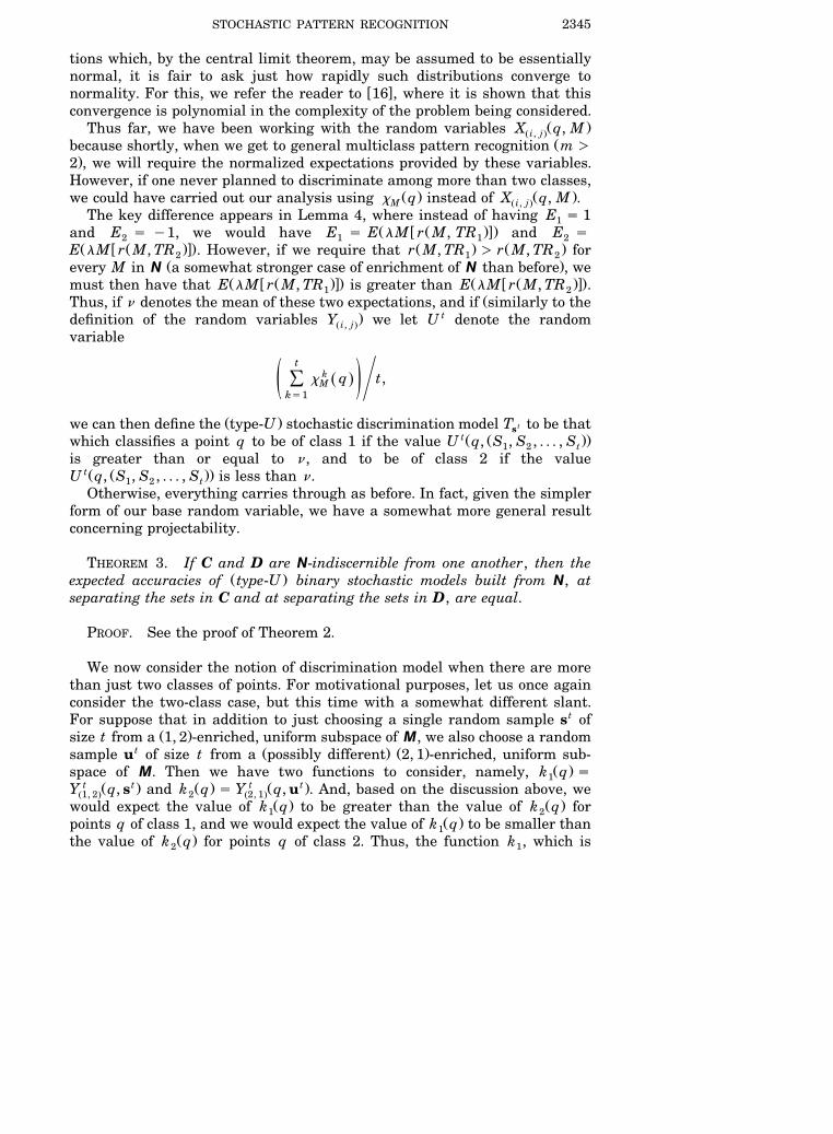
Ž . twe can then define the type-U stochastic discrimination model T to be thatstŽ Ž ..which classifies a point q to be of class 1 if the value U q, S , S , . . . , S1 2 t

is greater than or equal to n , and to be of class 2 if the valuetŽ Ž ..U q, S , S , . . . , S is less than n .1 2 tOtherwise, everything carries through as before. In fact, given the simpler

form of our base random variable, we have a somewhat more general resultconcerning projectability.

THEOREM 3. If C and D are N-indiscernible from one another, then theŽ .expected accuracies of type-U binary stochastic models built from N, at

separating the sets in C and at separating the sets in D, are equal.

PROOF. See the proof of Theorem 2.

We now consider the notion of discrimination model when there are morethan just two classes of points. For motivational purposes, let us once againconsider the two-class case, but this time with a somewhat different slant.For suppose that in addition to just choosing a single random sample st of

Ž .size t from a 1, 2 -enriched, uniform subspace of M, we also choose a randomt Ž . Ž .sample u of size t from a possibly different 2, 1 -enriched, uniform sub-

Ž .space of M. Then we have two functions to consider, namely, k q s1t Ž t . Ž . t Ž t .Y q, s and k q s Y q, u . And, based on the discussion above, weŽ1, 2. 2 Ž2, 1.

Ž . Ž .would expect the value of k q to be greater than the value of k q for1 2Ž .points q of class 1, and we would expect the value of k q to be smaller than1

Ž .the value of k q for points q of class 2. Thus, the function k , which is2 1

E. M. KLEINBERG2346

Žderived from a space of sets enriched with respect to points of class 1 at the.expense of points of class 2 , is a measure of the degree to which a given point

Ž .is 1-like the higher the value of k the more 1-like a point is , and the1function k , which is derived from a space of sets enriched with respect to2

Ž .points of class 2 at the expense of points of class 1 , is a measure of thedegree to which a given point is 2-like. So, to classify a given point q, we

Ž . Ž .would simply evaluate k q for 1 F i F 2, and if k q turned out to be thei ngreater of the two values, then n would be the classification we gave q.

In just this way, we will produce models for discriminating among manyclasses. Indeed, for any positive integer m, given an m-class discriminationproblem, we will produce functions k for each i between 1 and m, whereieach k will be based on a random sample from a space enriched with respecti

Ž .to points of class i. As before, k q will, in some sense, measure the degree toiwhich a given point q is i-like; given a point q, our discrimination model will

Ž .simply classify q as being of class i if k q is the largest value amongi� Ž . Ž . Ž .4k q , k 2 , . . . , k q .1 2 m

There are a number of ways in which we can produce these functions k .iFor example, we could deal simply with m subspaces of M where, for each i,

w Ž .x1 F i F m, the expectation of lM r M, TR restricted to the ith subspaceiw Ž .xwas greater than any of the expectations of the lM r M, TR for j notj

equal to i. However, given potential problems involved with achieving neu-trality in practical applications, a more refined and accurate approach in-volves carrying out all enrichment in terms of binary pairs. We proceed asfollows:

for any given pair of distinct integers i and j, assume that N is aŽ i, j.Ž . Ž . Žuniform, i, j -enriched, i, j -neutral subspace of M with TR N -indis-Ž i, j.

.cernible from TE , and assume that we have chosen a random sample,t Ž .s of size t from N . Then we have m m-1 functions, namely, theŽ i, j. Ž i, j.

w t Ž t .xfunctions lq Y q, s discussed above. We now define m new func-Ž i, j. Ž i, j.t tŽ .tions k by simply setting, for each i between 1 and m, k q equal toi i

mt tY q , s m y 1 .Ž .Ž .Ý Ž i , j. Ž i , j.� 0js1

j/i

The following points are now immediate from our earlier discussion: foreach i between 1 and m:

1. The expected value of the function k t, when it is restricted to points ofiŽ .class i, is 1 see Lemma 4 .

2. If n denotes the largest of the neutrality degrees nN for 1 F j F m,i Ž i, j.j / i, then the expected value of the function k t, when it is restricted toi

Ž . Žpoints of class other that i, is less than or equal to 2n y 1 - 1 seei.Lemma 4 .


3. The probability that k t deviates greatly from these expected values ap-iproaches 0 as t approaches `; the rate of this convergence is rapid in t.

4. These facts hold whether we view k t as being a function of points in theiunion of the TR , or a function of points in the union of the TE .i i

As a result, we may define our m-class discrimination model, E t, as follows:

tŽ .given any point q, evaluate k q for each i between 1 and m; find theitŽ . tŽ .least i such that k q is greater than or equal to k q for each j betweeni j

1 and m; now classify q as being of class i.

In light of our discussion above, the expected accuracy of this discriminationmodel E t can be made as high as desired by choosing t to be sufficientlylarge.

The reader might have noticed that from a theoretical point of view,multiclass discrimination could just as well have been carried out by simplydefining, for each i between 1 and m, k t to be Y t . However, giveni Ž i, Ž iq1.modŽm..the way we did define k t, there is what might be called a secondary stochasticieffect taking place here. For the essence of stochastic discrimination lies inthe fact that as one forms a random variable by taking a sum of independentrandom variables, the variance of that sum approaches 0 as the number ofcomponent variables approaches `. Thus, in the case of k t, a sum of m y 1ivariables, each of which is itself a sum of t variables, large values of mcontribute to the desired small variance just as do large values of t. Further-more, in practical applications, where both uniformity and neutrality aresometimes difficult to achieve, the impact from defining k t as the sum ofim y 1 random variables on ameliorating deficiencies in strict uniformity orneutrality is often significant.

5. A geometric interpretation of binary stochastic modeling. LetŽ .N be a fixed 1, 2 -enriched, uniform subspace of M. Let q be any given point

Ž .in F. Then by carrying out random sampling with replacement from N, wecan build a record of numeric fields associated with q by simply taking the

w Ž .xsequence of values of lM X q, M on successive points in the sample. InŽ1, 2.this way, we can map the original feature space F into higher and higher

Ž .dimensional Euclidean spaces in effect, new feature spaces , and we claimthat no matter how accurate a model one desires, if we go to a high enough

Ž .dimension, t, then the expectation is that some t y 1-dimensional hyper-plane in that Euclidean t-space would affect a model with that degree ofaccuracy. In other words, given a desired degree of accuracy, 1 y « , thereexists a t such that the expected accuracy of the discrimination model MHdetermined by some t y 1-dimensional hyperplane H in Euclidean t-space is

Žgreater than 1 y « . M classifies a point to be of class 1 if it is on one side ofH.H, and of class 2 if it is on the other side of H. In effect, we have a method

here for adding features so that models based on linear discriminant analysis

E. M. KLEINBERG2348

Ž .continue to increase in accuracy monotonically to any desired degree as wewincrease the number of features. Viewing our method in this way provides

another perspective on its virtue as a general tool for pattern recognition. ForŽ w x.as Bellman see 5 and others have demonstrated, adding features often

leads to a decrease in model projectability. Thus, this well-known ‘‘curse ofdimensionality’’ is completely reversed if one adds features as described

xabove.In order to see this, let t be a fixed positive integer, and let us consider,

t Ž .given a random sample s s S , S , . . . , S of size t from N, the embedding1 2 te t from F into Euclidean t-space which sends any q in F to the vector whoses

Ž . Ž . Ž .kth coordinate for 1 F k F t is equal to X q, S . Let H t denote theŽ i, j. kt y 1-dimensional hyperplane in Euclidean t-space which passes through theorigin and which is orthogonal to the vector n , all of whose coordinates aretequal to 1. Working with the metric on Euclidean t-space which results when

'one contracts the standard Euclidean metric by the factor 1r t , it is easy tosee that for any random sample st of size t from N, given a point q in F, the

Ž . Ž . t Ž t . wtsigned distance from e q to H t is equal to Y q, s . The sign of thes Ž1, 2.Ž .distance is ‘‘q’’ if q is on the same side of H t as the point n ; it is ‘‘y’’t

xotherwise. Thus, intuitively, the probability density function for the randomtw t Ž t .xvariable ls Y q, s really represents the probable locations where oneŽ1, 2.

wcan expect to find the point q in Euclidean t-space vis-a-vis its distance from`Ž .xthe hyperplane H t after q is passed through a ‘‘generic’’ embedding. In

light of our discussion above concerning the accuracy of binary stochasticmodels, we see that the density function g t

T R1 portrays the distribution ofsŽ .points in TR with respect to their signed distance from the hyperplane H t ,1

and the function g tT R 2 portrays the distribution of points in TR with respects 2

Ž .to their signed distance from H t .By the central limit theorem, as t increases, we can think of g t

T R1 andsg t

T R 2 as normal functions with variances inversely proportional to t, and sincesthese functions are centered at 1 and y1, respectively, we see, given ourprevious discussion, that as t increases without bound, the likelihood of

Ž .finding members of F of like class on opposite sides of the hyperplane H tdecreases to 0. Thus, as t approaches `, the expected accuracy of such ahyperplane-based discrimination model goes to 1. In fact, the hyperplane-

Ž .based model M which classifies a point q to be of class 1 2 if the sign ofH Ž t .Ž . Ž . Ž .t tthe distance of e q to H t is ‘‘q’’ ‘‘y’’ is identical to the model Ms s

defined in Section 4.

Acknowledgments. The author wishes to thank R. Berlind, T. Biehler,D. Bowen and T. K. Ho for their useful comments based on preliminaryversions of this paper. Many of their suggestions have been included here. Inaddition, Dr. Ho provided access to many of the data sets used in this paper.Her help in dealing with these, as well as in supplying nearest-neighborresults included in this paper, in writing the graphical tools used in produc-ing the pictures of Section 2, and, in general, with supplying perspectiverelating our methods to more traditional methods, is greatly appreciated. We


also wish to thank E. G. Kleinberg for sharing many helpful insights and fortechnical assistance in producing some of the neural network results dis-cussed here. Finally, we thank L. D. Brown for his patient help in suggestingmany revisions of our original manuscript.

REFERENCES

w x Ž .1 AMIT, Y., GEMAN, D. and WILDER, K. 1996 . Recognizing shapes from simple queries aboutgeometry. Unpublished manuscript.

w x Ž .2 BERLIND, R. 1994 . An alternative method of stochastic discrimination with applications topattern recognition. Ph.D. dissertation, Dept. Mathematics, State Univ. New York,Buffalo.

w x Ž .3 BERLIND, R. 1994 . Almost uniformity in stochastic modeling. Unpublished manuscript.w x Ž .4 COVER, T. M. and HART, P. E. 1967 . Nearest neighbor pattern classification. IEEE Trans.

Inform. Theory IT-13 21]27.w x Ž .5 DUDA, R. O. and HART, P. E. 1973 . Pattern Classification and Scene Analysis. Wiley, New

York.w x Ž .6 FREUND, Y. 1995 . Boosting a weak learning algorithm by majority. Inform. and Comput.

121 256]285.w x Ž .7 GEMAN, S., BIENENSTOCK, E. and DOURSAT, R. 1992 . Neural networks and the biasrvari-

ance dilemma. Neural Computation 4 1]58.w x Ž .8 GOLDMAN, S. A., KEARNS, M. J. and SCHAPIRE, R. E. 1995 . On the sample complexity of

weakly learning. Inform. and Comput. 117 276]287.w x Ž .9 GUYON, I. 1991 . Applications of neural networks to character recognition. In Character

Ž .and Handwriting Recognition P. S. P. Wang, ed. . World Scientific, Singapore.w x Ž .10 HARALICK, R. M. 1976 . The table look-up rule. Comm. Statist. Theory Methods 5 1163]1191.w x Ž .11 HECHT-NIELSEN, R. 1990 . Neurocomputing. Addison-Wesley, Reading, MA.w x Ž .12 HO, T. K. 1992 . A theory of multiple classifier systems and its application to visual word

recognition. Ph.D. thesis, Dept. Computer Science, State Univ. New York, Buffalo.w x Ž .13 HO, T. K. 1993 . Recognition of handwritten digits by combining independent learning

vector quantizations. In Proceedings of the Second International Conference on Docu-Ž .ment Analysis and Recognition M. Kavanaugh, ed. 818]821. IEEE Computer Society

Press, New York.w x Ž .14 HO, T. K. 1995 . Random decision forests. In Proceedings of the Third International

ŽConference on Document Analysis and Recognition M. Kavanaugh and P. Storms,.eds. 278]282. IEEE Computer Society Press, New York.

w x Ž .15 KANAL, L. 1974 . Patterns in pattern recognition: 1968]1974. IEEE Trans. Inform. TheoryIT-20 697]722.

w x Ž .16 KLEINBERG, E. M. 1990 . Stochastic discrimination. Annals of Mathematics and ArtificialIntelligence 1 207]239.

w x Ž .17 KLEINBERG, E. M. and HO, T. K. 1993 . Pattern recognition by stochastic modeling. InProceedings of the Third International Workshop on Frontiers in Handwriting Recog-

Ž .nition M. Bosker, R. Casey, et al., eds. 175]183. Partners Press, Buffalo, NY.w x Ž .18 KLEINBERG, E. M. and HO, T. K. 1996 . Building projectable classifiers of arbitrary com-

plexity. In Proceedings of the 13th International Conference on Pattern RecognitionŽ .M. E. Kavanaugh and B. Werner, eds. 880]885. IEEE Computer Society Press, NewYork.

w x Ž .19 PROJECT STATLOG 1992 . LIACC. Univ. Porto. Internet address: ftp.ncc.up.pt:pubrstatlogrdatasets.

w x Ž .20 SCHAPIRE, R. E. 1990 . The strength of weak learnability. Machine Learning 5 197]227.

DEPARTMENT OF MATHEMATICS

STATE UNIVERSITY OF NEW YORK

BUFFALO, NEW YORK 14214E-MAIL: [email protected]

Documents

AN OVERTRAINING-RESISTANT STOCHASTIC MODELING …