3

BULGARIAN ACADEMY OF SCIENCES

CYBERNETICS AND INFORMATION TECHNOLOGIES Volume 17, No 1

Sofia 2017 Print ISSN: 1311-9702; Online ISSN: 1314-4081

DOI: 10.1515/cait-2017-0001

An Optimization of Closed Frequent Subgraph Mining

Algorithm

J. Demetrovics1, H. M. Quang2, N. V. Anh2, V. D. Thi3 1Computer and Automation Institute Hungarian Academy of Sciences, Hungary 2Institute of Information Technology, Vietnam Academy of Science and Technology, Viet Nam 3The Information Technology Institute (ITI), Vietnam National University, Hanoi, Viet Nam

Emails: demetrovics@sztaki.mta.hu hoangquang@ioit.ac.vn anhnv@ioit.ac.vn vdthi@vnu.edu.vn

Abstract: Graph mining is a major area of interest within the field of data mining in

recent years. A key aspect of graph mining is frequent subgraph mining. Central to

the entire discipline of frequent subgraph mining is the concept of subgraph

isomorphism. One major issue in early subgraph isomorphism research concerns

computational complexity. Normally, the subgraph isomorphism problem is

NP-complete. Previous studies of frequent subgraph mining have not solved

NP-complete problem in the subgraph isomorphism. In this paper, we propose a

new algorithm which can deal with this problem. The proposed algorithm can solve

the subgraph isomorphism in polynomial time in some settings. Moreover, the new

algorithm is proved theoretically more effective than previous studies in closed

frequent subgraph mining.

Keywords: Frequent patterns, closed frequent subgraph, frequent subgraphs,

subgraph mining, subgraph isomorphism.

1. Introduction

Data mining is a process for extracting knowledge from data. The data can be

represented in many formats of structured data such as tables [1, 13], graphs [11],

etc. Graph mining is recently a major area of interest within the field of data

mining. A key aspect of graph mining is frequent subgraph mining. Frequent

patterns are itemsets, subsequences, or substructures that appear in a data set with

frequency no less than a user-specified threshold [4]. A substructure can refer to

different structural forms, such as subgraphs, subtrees, or sublattices, which may be

combined with itemsets or subsequences. If a substructure occurs frequently in a

graph database, it is called a frequent structural pattern. Finding frequent patterns

plays an essential role in mining associations, correlations, and many other

interesting relationships among data. Moreover, it helps in data indexing,

classification, clustering, and other data mining tasks as well. Thus, frequent pattern

4

mining has become an important data mining task and a focused theme in data

mining research.

Generally, Frequent Subgraph Mining (FSM) aims to identify all subgraph

patterns whose occurrences within a graph data set are above a user defined

threshold. These subgraph patterns are called frequent subgraphs. Theoretically,

frequent subgraph mining can be formulated as a search in a search space, modelled

by a lattice, consisting of all possible subgraph patterns. Because the number of

possible frequent subgraphs increases exponentially with the size of the graph,

traversing the search space completely is computationally intractable, because of a

“combinatorial explosion”. Thus, a user specified support threshold is often used to

prune this combinatorial search space, i.e., to separate infrequent subgraphs from

the frequent ones. Frequent subgraph mining problem has received considerable

critical attention [6, 8, 9, 17, 18]. It is widely accepted that FSM techniques can be

divided into two categories: (i) the “A priori-based” approach (also called the BFS

strategy based approach) [8] and (ii) the pattern growth approach [17]. Both

approaches have advantages and disadvantages; however, they include generating

candidate and isomorphism subgraph testing to decide which subgraph is frequent.

In theoretical computer science, the subgraph isomorphism problem is a

computational task in which two graphs G and H are given as input, and it has to be

determined whether G contains a subgraph that is isomorphic to H. Subgraph

isomorphism is a generalization of both the maximum clique problem and the

problem of testing whether a graph contains a Hamiltonian cycle, and is therefore

NP-complete [3] However certain other cases of subgraph isomorphism may be

solved in polynomial time [2, 5] for planar graphs.

A considerable amount of literature has been published on subgraph

isomorphism in frequent subgraph mining problem [2, 5, 6, 10, 15]. These studies

help to reduce time complexity of subgraph isomorphism. The use of adjacency

matrices, although straightforward, does not lend itself to isomorphism detection,

because the vertexes (and edges) can be enumerated in many different ways [16].

With respect to isomorphism testing, it is therefore desirable to adopt a consistent

labelling strategy that ensures that any two identical graphs are labelled in the same

way regardless of the order in which vertexes and edges are presented (i.e., a

canonical labelling strategy). A canonical labelling strategy defines a unique code

for a given graph [11]. Canonical labelling facilitates isomorphism checking

because it ensures that if a pair of graphs is isomorphic, then their canonical

labellings will be identical [9]. One simple way of generating a canonical labelling

is to flatten the associated adjacency matrix by concatenating rows or columns to

produce a code comprising a list of integers with a lexicographical ordering

imposed. To further reduce the computation resulting from the permutations of the

matrix, canonical labellings are usually compressed, using what is known as a

vertex invariant scheme [11]; this allows the content of an adjacency matrix to be

partitioned according to the vertex labels.

Alternative methods to reducing the search space include concentrating on the

identification of a subset of the total set of frequent subgraphs, for example, closed

frequent subgraph mining [18] or maximal frequent subgraph mining [7, 14].

5

Although these methods address the issue to some extent, the combinatorial

explosion issue is still unresolved; significantly large numbers of closed frequent

subgraphs and maximal frequent subgraphs are still generated.

In this paper, we propose new algorithm for closed frequent subgraph mining

based on canonical labelling strategy, the Random Access Machine (RAM) model

or von Neumann model [12] and the “A priori-based” approach. The RAM makes

use of a random access memory, thus overcoming the limitation of Turing machines

which use a sequential access tape as a memory component. The RAM that can

access any field of their memory in one step has to know which cell to access, and

each cell must be assigned an address. The subgraph isomorphism problem with

canonical labelling strategy is defined by searching an element in an array

according to code string and can utilize binary search on RAM. In the proposed

algorithm, the subgraph isomorphism problem solve in polynomial time

complexity. As far we know the subgraph isomorphism problem has not been

considered in the random access machine model. This paper attempts to show that

the new algorithm is faster than some algorithms in [6, 8, 9, 17, 18]. In addition,

this paper also shows the correctness and gives the time complexity of the new

algorithm.

2. Preliminaries

Definition 2.1. A labelled graph G is five element tuple ( , , , , ),V E

G V E l

where V is a set of vertices, E V V is a set of edges. V

and E

are the set

of vertex labels and edge labels respectively. The labelling function l defines the

mappings V

V and .E

E

Definition 2.2. Without loss of generality, we assume that there is a total order

≥ on each label set V

and .E

A graph ( , , , , )V E

G V E l is a subgraph of

other graph ( , , , , )V E

G V E l

if

(1) ,

(2) , ( ( ) ( )),

(3) ,

(4) ( , ) , ( ( , ) ( , )),

V V

u V l u l u

E E

u v E l u v l u v

G' is also referred to as a supergraph of G.

Definition 2.3. Two graphs ( , , , , ),V E

G V E l ( , , , , )V E

G V E l

are

isomorphic if there exists a bijection :f V V such that:

6

(1) , ( ( ) ( ( )));

(2) , , (( , ) ) ( ( ), ( )) ;

(3) ( , ) , ( ( , ) ( ( ), ( )).

u V l u l f u

u v V u v E f u f v E

u v E l u v l f u f v

Definition 2.4. A labelled graph G is subgraph isomorphism to a labelled

graph G', denoted by G ⊆ G', if there exists a subgraph G" of G' such that G is

isomorphic to G".

Definition 2.5. Given a set of graphs GD (referred as a Graph Database) and a

threshold σ (0 ≤ σ ≤ 1), the support of a graph G, denoted by supG is defined as the

fraction of graphs in GD to which G is subgraph isomorphic of G':

{ GD }sup .

GDG

G G G

∣

∣ ∣

G is frequent if supG ≥ σ.

Definition 2.6. The frequent subgraph mining problem is given a threshold σ

and a graph database GD, finding all frequent subgraphs in GD.

Definition 2.7. A set consisting of all Frequent Subgraphs of graph g denoted

as FS(g).

Definition 2.8. If g is a subgraph of g', then g' is a supergraph of g, denoted

by g ⊆ g' (proper supergraph, if g ⊂ g'). Let FS be the set of

frequent subgraphs, the set of closed frequent subgraphs, CS, is defined

CS { | FS, FS: and sup sup }.g gg g g g g

Definition 2.9. A k-subgraph of graph g is a subgraph g' ⊆ g such that |Vg'|=k.

Definition 2.10. Given an n n adjacency matrix M of a graph G with n

vertices, we define the code of M, denoted by code(M), as the sequence formed by

concatenating lower triangular entries of M (including entries on the diagonal) in

the order: 1,1 2,1 2,2 ,1 ,2 , 1 ,... ...n n n n n nm m m m m m m where mi,j is the entry at the i-th row and

j-th column in M (0 ).j i n We assume that the rows in M are numbered 1

through n from top to bottom and the columns are numbered 1 through n from left

to right.

3. The PSI-CFSM algorithm

In this paper, we propose a method about optimization computation for subgraph

isomorphism in frequent subgraph mining. The proposed method is proved

theoretically faster than gSpan [17] and FFSM [6]. A graph will be represented

uniquely with a code by using canonical labelling, lexicographic order similar to

MDFS-C [17, 18] and CAM [6, 8, 9]. The unique representation of a graph with a

code of CAM or MDFS-C will avoid duplication generating of subgraphs and can

help to construct ordered array that contain subgraphs in code of MDFS-C of CAM.

Furthermore, the test subgraph isomorphism described as follow can utilize binary

search in random access machine model. We consider subgraph isomorphism

problem that is to match a pair of two subgraph. This problem is equivalence to

comparing a pair of strings that are codes of MDFS-C of CAM representation of the

7

two subgraphs. The time complexity of binary search is O(log n) where n is the size

of the input ordered array. The algorithm is called Polynomial Subgraph

Isomorphism Closed Frequent Subgraph Mining (PSI-CFSM). It uses “A priori-

based” approach and random access machine model. According to “A priori-based”

approach, the frequent subgraph mining process starts from level one that generates

a set 2

iC of 2-subgraph (subgraphs have two nodes or only one edge) candidates of

each graph Gi in graph database GD. It then tests 2-subgraph isomorphism and

counts support each of the set 2

iC to find a set of frequent 2-subgraphs of graph Gi,

a set of frequent 2-subgraphs of GD, a set of closed frequent 2-subgraph of Gi and a

set of closed frequent 2-subgraph of GD which are denoted as 2FSi ,

2FS , 2CSi and

2CS , respectively. The next process is a loop with k ≥ 3 that generates a set i

kC of

candidate k-subgraphs (subgraphs having k nodes can contain more than k–1 edges

and less than (k(k–1)/2) edges) of Gi from the set of frequent 2-subgraph 2FSi

combined with the set of frequent (k–1)-subgraphs 1FSk

i

. It then tests k-subgraph

isomorphism and counts support of k-subgraph of i

kC to find a set of frequent

k-subgraphs of Gi, a set of frequent k-subgraphs of GD, a set of closed frequent

k-subgraphs of Gi and a set of closed frequent k-subgraphs of GD denoted as FSk

i ,

FSk, CSk

i and CSk, respectively. In this process at k, every k-subgraph of CSk

i and

CSk is constructed with a linked list containing (k–1)-subgraph of

1FSk

i

and

1FSk, respectively. The algorithm checks each k-subgraph of CSk

i and CSk such

that the k-subgraph contains (k–1)-subgraph of 1CSk

i

and

1CSk in their linked list

and removes identified (k–1)-subgraphs in 1CSk

i

and

1CSk, respectively. The loop

process stops when no candidate k-subgraph is generated. The set of union sets CS1,

CS2, ..., CSk is the set of closed frequent subgraphs. We can see that k-subgraph

isomorphism testing process is to find a code of unique representation of

k-subgraph in an ordered array in which each element containing a code of unique

representation of k-subgraph in the k-subgraphs set. Subgraph isomorphism testing

process uses binary search in random access machine to reduce time complexity to

polynomial. Hence, the PSI-CFSM algorithm is faster than gSpan, FFSM and FSG

algorithms in running time.

3.1. Canonical labelling strategy

Fig. 1. A sample graph database GD

8

Minimum DFS Code (M-DFSC): There are a number of variants of the Depth

First Search (DFS) code canonical labelling scheme; but essentially each vertex is

given a unique identifier generated from a DFS traversal of the graph (DFS

subscripting). Each constituent edge of the graph in the DFS code is then

represented by a 5-tuple: (i, j, li, le, lj), where i and j are the vertex identifiers, li and

lj are the labels for the corresponding vertexes, and le is the label for the edge

connecting the vertexes. Based on the DFS lexicographic order, the M-DFSC of a

graph g is defined as the canonical labelling of g [17, 18]. The DFS codes for the

left-most branch and the right-most branch of the example graph G given in

Fig. 1. (g1) are {(0, 1, x, a, x), (1, 2, x, a, z), (2, 3, z, d, z)} and {(0, 1, x, a, x),

(1, 4, x, b, y), (4, 5, y, c, z)}, respectively.

Canonical Adjacency Matrix (CAM): Given an adjacency matrix M of a graph

g, an encoding of M can be obtained by the sequence of concatenating lower

(or upper) triangular entries of M, including entries on the diagonal. Since different

permutations of the set of vertexes correspond to different adjacency matrices,

the canonical (CAM) form of g is defined as the maximal (or minimal) encoding.

The adjacency matrix from which the canonical form is generated defines

the Canonical Adjacency Matrix or CAM [6, 8, 9]. The encoding for the example

graph G given in Fig. 1. (g1), represented by the canonical adjacency matrix have

code(CAM(g1)) = xaxabzabdzbb00yc000cz.

3.2. Generate subgraph candidates

gSpan [17] developed an efficient way to reduce the total number of nodes need to

be considered. In gSpan, the extension operation is only performed to nodes on the

“rightmost path” of a graph. Given a graph g and one of its depth first search trees

T, the rightmost path of g with respect to T is the rightmost path of the tree T. gSpan

chooses only one depth first search tree T which produces the canonical form of g

for extension. gSpan extents one edge to right most path to receive (k+1)-subgraph

from k-subgraph (k-subgraph in gSpan means that the subgraph have k edges).

The FFSM [6] algorithm uses two procedures FFSM_Extension and

FFSM_Join to generate candidate subgraphs. FFSM_Join combines two

k-subgraphs to generate (k+1)-subgraphs if the two k-subgraphs sharing a common

(k–1)-subgraph (k-subgraph in FFSM means that the subgraph have k edges) and

the FFSM_Join does not generate unique (k+1)-subgraphs from the two

k-subgraphs. FFSM_Extension improves the efficient gSpan by always choosing a

single fixed node in a CAM and attaches a newly introduced edge to it together with

an additional node.

In the proposed algorithm, PSI-CFSM, we use an enumeration technique that

is an extension operation to construct a (k+1)-subgraph candidate g from a

k-subgraph graph of Gi by adding additional edges (the k-subgraph means that the

subgraph have k nodes). The newly introduced edge might connect two existing

nodes or connect an existing node with a node introduced together with the edge. A

simple way to perform the extension operation is to introduce every possible edge

to every node in a graph g. This method has clearly a polynomial time complexity

for the set of available vertex- and edge- labels for a graph g, respectively.

9

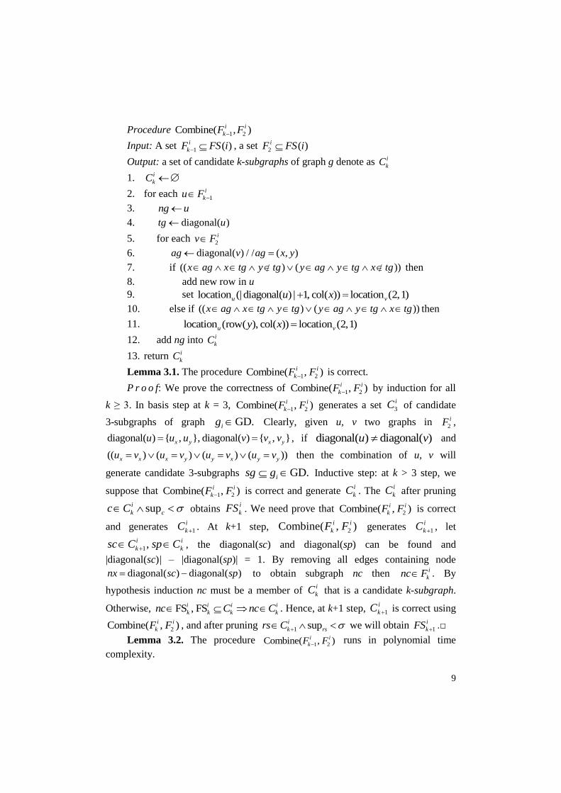
Procedure 1 2Combine( , )i i

kF F

Input: A set 1 ( )k

iF FS i , a set 2 ( )iF FS i

Output: a set of candidate k-subgraphs of graph g denote as i

kC

1. i

kC

2. for each 1

i

ku F

3. ng u

4. diagonal( )tg u

5. for each 2

iv F

6. diagonal( ) / / ( , )ag v ag x y

7. if (( ) ( ))x ag x tg y tg y ag y tg x tg then

8. add new row in u

9. set location (| diagonal( ) | 1, col( )) location (2,1)u vu x

10. else if (( ) ( ))x ag x tg y tg y ag y tg x tg then

11. location (row( ), col( )) location (2,1)u vy x

12. add ng into i

kC

13. return i

kC

Lemma 3.1. The procedure 1 2Combine( , )i i

kF F is correct.

P r o o f: We prove the correctness of 1 2Combine( , )i i

kF F by induction for all

k ≥ 3. In basis step at k = 3, 1 2Combine( , )i i

kF F generates a set 3

iC of candidate

3-subgraphs of graph GD.ig Clearly, given u, v two graphs in 2

iF ,

diagonal( ) { , }, diagonal( ) { , }x y x yu u u v v v , if diagonal( ) diagonal( )u v and

(( ) ( ) ( ) ( ))x x x y y x y yu v u v u v u v then the combination of u, v will

generate candidate 3-subgraphs GD.isg g Inductive step: at k > 3 step, we

suppose that 1 2Combine( , )i i

kF F is correct and generate

i

kC . The i

kC after pruning

supi

k cc C obtains i

kFS . We need prove that 2Combine( , )i i

kF F is correct

and generates 1

i

kC . At k+1 step, 2Combine( , )i i

kF F generates 1

i

kC , let

1,i i

k ksc C sp C , the diagonal(sc) and diagonal(sp) can be found and

|diagonal(sc)| – |diagonal(sp)| = 1. By removing all edges containing node

diagonal( ) diagonal( )nx sc sp to obtain subgraph nc then i

knc F . By

hypothesis induction nc must be a member of i

kC that is a candidate k-subgraph.

Otherwise, FS , FSi i i i

k k k knc C nc C . Hence, at k+1 step, 1

i

kC is correct using

2Combine( , )i i

kF F , and after pruning 1 supi

k rsrs C we will obtain 1

i

kFS .□

Lemma 3.2. The procedure 1 2Combine( , )i i

kF F runs in polynomial time

complexity.

10

P r o o f: Let m is the number of edges of a subgraph 1

i

kg F ,

| diagonal( ) | 1g k , | diagonal( ) | 1 2m g k , n is cardinality of 2

iF (each

subgraph in 2

iF contains only one edge), h is cardinality of 1

i

kF , before adding one

node to (k – 1)-subgraph g to obtain k-subgraph g' then the number of maximal

nodes can be add to g is | | | diagonal( ) |igV g . By CAM representation, the number

of edges of g maximum is ( 2) ( 3)

2

k k . Assume that each subgraph 1

i

kg F

can be added maximum number of edges when generating candidate

k-subgraph i

kg C then the number of edges can be added to g is (k – 1). Thus, the

procedure 1 2Combine( , )i i

kF F has maximum number of computation step that is

(| | ( 1)) ( 1)igh V k k . In our algorithm, we focus in closed frequent subgraph

mining, we use the procedure 1 2Combine(CS , FS )i i

k to generate the set of candidate

k-subgraphs i

kC and the cardinality of i

kC is much less than using

1 2Combine(FS , FS )i i

k.□

3.3. Test subgraph isomorphism

In algorithms [6, 8, 9, 17, 18] the subgraph isomorphism testing process runs in a

sequence way. Therefore, a new candidate subgraph g generated by right most path

extension (gSpan) [17] or by joining (FFSM) [6] must test subgraph isomorphism

with every graph GDig g . The subgraph isomorphism testing process

compares code of MDFS-C or CAM of one candidate subgraph g with every

subgraph GDig g in a set of very large subgraphs of graph GDig .

Assume the number of subgraphs of graph GDig is 2n then the process implies

2n comparison step. We can easily see why the process runs slow. Hence, subgraph

isomorphism testing step of algorithms such as FFSM, gSpan, CloseGraph has the

time complexity in NP class.

We improve subgraph isomorphism testing step of the above algorithms by

using a random access machine model in binary search. In the complexity theory,

the time complexity of binary search is (log )O n where n is number of candidate

subgraphs. Assume the cardinality of candidate subgraphs is 2n then number of

computation steps of subgraph isomorphism by binary search on random access

machine model is 2log 2n n and the time complexity is ( )O n .

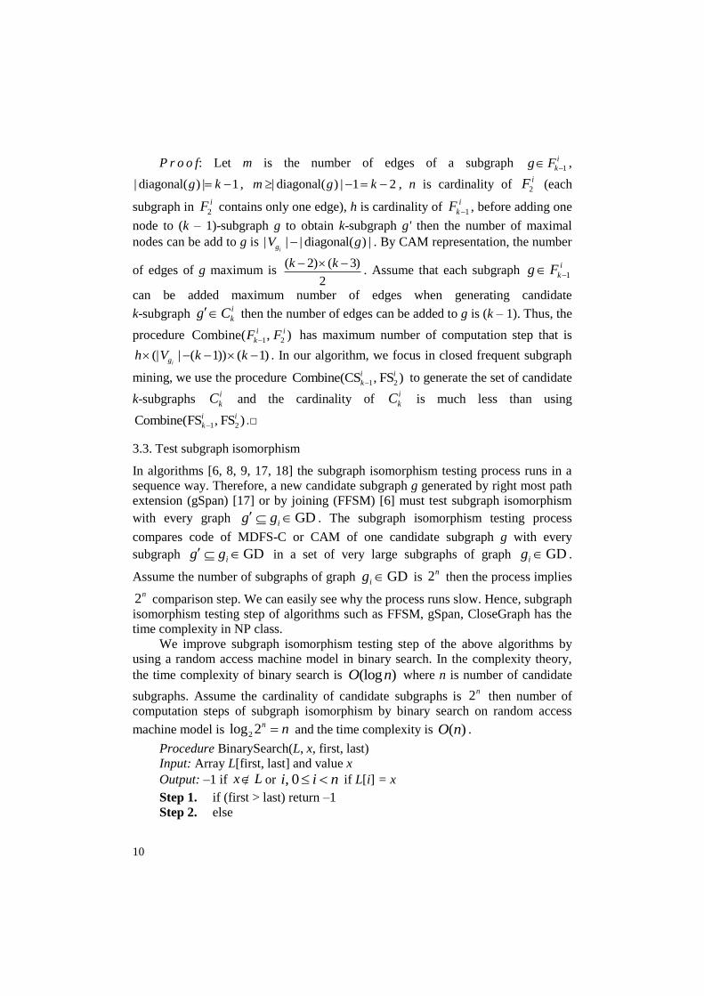
Procedure BinarySearch(L, x, first, last)

Input: Array L[first, last] and value x

Output: –1 if x L or , 0i i n if L[i] = x

Step 1. if (first > last) return –1

Step 2. else

11

Step 3. first last

middle2

Step 4. if (L[middle]=x) return middle

Step 5. else if (L[middle]<x) return BinarySearch(L, x, middle+1, last)

Step 6. else return BinarySearch(L, x, first, middle – 1)

Lemma 3.3. The procedure BinarySearch(L, x, first, last) runs in time

complexity O(logn).

P r o o f: Let T(n) is the number of computation steps that algorithm

BinarySearch needs to perform when the size of the input is n. At n=0 we have

T(0) = c', where c' is constant and |L|=0, the procedure just performs a constant

number of computation steps. At n > 0, the procedure performs a constant number c

of computation steps to find the element in the middle of L, compares that element

with x and defines the range on the left half or on the right half of the array L for

recursion. Assume that both halves of the array L have the same size, (n–1)/2.

Hence, the total number of computation steps BinarySearch performs when n > 0 is

T(n) = c + T((n–1)/2). The recurrence equation as follow:

(0)T c

(3.3.1) 1

( )2

nT n c T

if n > 0,

0 1

2 2

11

1 1 2 2 22

2 2 2 2

n

n n nT c T c T c T

,

0 1 0 1 1

1 2

2 2 ...2 2 2 ...2

2 2

k

k

k

k

n nT c T

.

The procedure will stop whenever the argument is equal to zero:

(3.3.2) 0 1 1

2

2 2 ...20

2

k

k

n

;

(3.3.3) 0 1 1

2

2 2 ...2( ) ...

2

k

k

nT n c c c f

.

The set of Equations (3.3.1) has k+2 equations, the number of c terms in

(3.3.3) is k+2 and so T(n) = (k+2)c + c'. According to the fact that (3.3.2):

(3.3.4) 1

0 1 1 1

0

2 2 ... 2 2 2 1k

k i k

i

n

.

Therefore, taking logarithms on the both sides of the last equality (3.3.4) we

obtain 22 log ( 1)k n . Then,

2( ) clog ( 1)T n n c .

Ignoring constant terms, we finally conclude that T(n) = O(logn). □

Lemma 3.4. The procedure BinarySearch(L, x, first, last) is correct

P r o o f: We need to prove that 0n , BinarySearch(L, x, first, last) returns

a range in sorted array L with 0 first last | |L if value x is in sorted array L.

12

Basis step: At n=0 step, sorted array L contains a range from 0 to |L|–1

BinarySearch(L, x, 0, |L|–1) returns the range [0, | | 1] [0, | | 1]L L for searching

x. Clearly, value x is in the range [0, |L| –1] of L, [0] [| | 1]L x L L .

Inductive step: Suppose that at n ≥ 0 step and BinarySearch(L,x,firstn,lastn)

returns the range [first , last ] [0, | | 1]n n L for searching x,

[first ] [last ]n nL x L .

We need to prove that at n + 1 step BinarySearch(L, x, first(n+1), last(n+1)) must

returns the range ( 1) ( 1)[first , last ] [0, | | 1]n n L for searching x,

( 1) ( 1)[first ] [last ]n nL x L .

BinarySearch(L, x, first(n+1), last(n+1)) returns [first(n+1), last(n+1)]:

(3.4.1) [first ] [last ]n nL x L (hypothesis induction)

In case 1:

(3.4.2) first last

2

n nL x

,

( 1) ( 1)

first last[first , last ] 1, last

2

n nn n n

.

By (3.4.1), (3.4.2) first last

1 [last ]2

n nnL x L

,

(3.4.3) ( 1) ( 1)[first ] [last ]n nL x L .

In case 2:

(3.4.4) first last

2

n nL x

,

( 1) ( 1)

first last[first , last ] first , 1

2

n nn n n

.

By (3.4.1), (3.4.4) first last

[first ] 12

n nnL x L

,

(3.4.5) ( 1) ( 1)[first ] [last ]n nL x L .

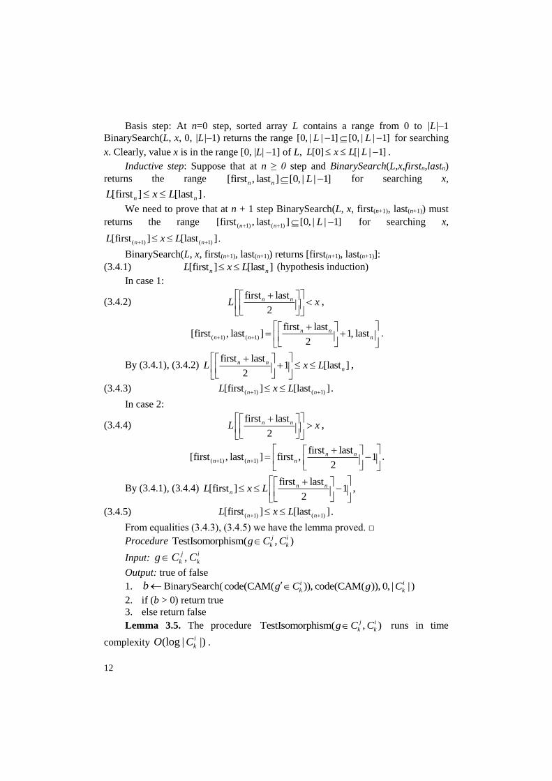
From equalities (3.4.3), (3.4.5) we have the lemma proved. □

Procedure TestIsomorphism( , )j i

k kg C C

Input: ,j i

k kg C C

Output: true of false

1. bBinarySearch( code(CAM( )), code(CAM( )), 0, | |i i

k kg C g C )

2. if (b > 0) return true

3. else return false

Lemma 3.5. The procedure TestIsomorphism( , )j i

k kg C C runs in time

complexity (log | |)i

kO C .

13

P r o o f : This is evident by Lemma 3.3.

Lemma 3.6. The procedure TestIsomorphism( , )j i

k kg C C is correct.

P r o o f : This is evident by Lemma 3.4.

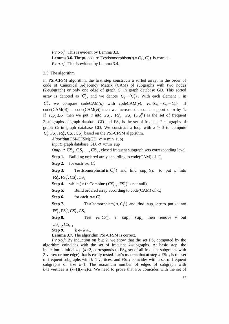
3.5. The algorithm

In PSI-CFSM algorithm, the first step constructs a sorted array, in the order of

code of Canonical Adjacency Matrix (CAM) of subgraphs with two nodes

(2-subgraph) or only one edge of graph Gi in graph database GD. This sorted

array is denoted as 2

iC , and we denote 2 2{ }iC C . With each element u in

2

iC , we compare codeCAM(u) with codeCAM(v), 2 2 2{ }j iv C C C . If

code(CAM(u)) = code(CAM(v)) then we increase the count support of u by 1.

If supu then we put u into 2FS ,

2FSi . 2FS (

2FSD ) is the set of frequent

2-subgraphs of graph database GD and 2FSi is the set of frequent 2-subgraphs of

graph Gi in graph database GD. We construct a loop with k ≥ 3 to compute

, FS , FS , CS , CSi i i

k k k k kC based on the PSI-CFSM algorithm.

Algorithm PSI-CFSM(GD, = min_sup)

Input: graph database GD, =min_sup

Output: 2 3CS , CS , ..., CSk , closed frequent subgraph sets corresponding level

Step 1. Building ordered array according to code(CAM) of 2

iC

Step 2. for each 2

iu C

Step 3. TestIsomorphism( 2, ju C ) and find supu to put u into

2 2 2 2FS , FS , CS , CSi D i

Step 4. while ( i : Combine (1 2CS , FSi i

k) is not null)

Step 5. Build ordered array according to code(CAM) of i

kC

Step 6. for each k

iu C

Step 7. TestIsomorphism( , k

ju C ) and find supu to put u into

FS , FS , , CSCSk k k

i D i

k

Step 8. Test 1

i

kv CS if sup supv u then remove v out

1 1, CS SC k

i

k

Step 9. 1k k

Lemma 3.7. The algorithm PSI-CFSM is correct.

P r o o f: By induction on k ≥ 2, we show that the set FSk computed by the

algorithm coincides with the set of frequent k-subgraphs. At basic step, the

induction is initialized (k=2, corresponds to FS2, set of all frequent subgraphs with

2 vertex or one edge) that is easily tested. Let’s assume that at step k FSk–1 is the set

of frequent subgraphs with k–1 vertices, and FSk–1 coincides with a set of frequent

subgraphs of size k–1. The maximum number of edges of subgraph with

k–1 vertices is (k–1)(k–2)/2. We need to prove that FSk coincides with the set of

14

frequent subgraphs of size k. For the inductive step, it is sufficient to prove that

given an arbitrary frequent subgraphs X of size k, X is surely included in the set FSk.

Thus, X is also a member of set FSi

k of k-subgraphs of one graph gi in graph

database GD. FSi

k is obtained by pruning step that removes candidate k-subgraphs

supi

k rr C where i

kC is output of Combine(1 2CS , FSi i

k). Then

Combine(1 2CS , FSi i

k) is correct by Lemma 3.1. Hence, FSk contains X and

coincides with the set of frequent subgraphs of size k.

We now consider the time complexity of PSI-CFSM algorithm. We suppose

that the cardinality of graph database GD is n and each computation step is

constant 1. At line 1, the number of computation steps is cardinality of all edges of

all graphs in graph database GD 1

GD

| CS | (| | ( 1)) ( )| | 1i

i

i

i

kg g

g

V k kE

. At

line 2 and 3, the number of steps is 2

GD GD

| | log | |i i

i i

g g

g g

E E

. From line 4 to

line 9 is a loop which has k steps. Line 4 runs the procedure Combine that has

1| CS | (| | ( 1)) ( 1)i

i

k gV k k steps. Thus, at line 5 the number of computation

steps is GD

1| CS | (| | ( 1)) |( 1) |i

i

i

k kg

i

g

V k k C

. In the similar way

2-subgraphs computation is initialized; at line 5, 6, 7, 8 and 9 the number of

computation steps is

1 2

GD GD

| | log | || CS | (| | ( 1)) ( 1)i

i

i

i i

k k

i

g g

k g C CV k k

.

Assume that every graph gi in graph database GD has | | 3igV then the

number of computation steps from line 1 to line 3 is too small in comparing from 4

to 9. Hence, the total number of computation steps in time complexity of the PSI-

CFSM algorithm is max(| |)

2

1 GD GD

1| CS | (| | ( 1)) ( | | log |1) |g

i

i

i

i

V

i i

k k

k g g

i

k gV k k C C

.

4. Conclusion

In this paper, we introduce an efficient method to reduce subgraph isomorphism

testing process. The proposed method obtains polynomial time complexity in closed

frequent subgraph mining. The subgraph isomorphism problem has time complexity

in NP class in the current state-of-the-art frequent subgraph mining algorithms. To

obtain polynomial time complexity in subgraph isomorphism, we use binary search

to find string code of unique representation of a k-subgraph in an ordered unique

string code array of a k-subgraph set in a random access machine model. In future,

15

we will continue this study by applying parallel mining to increase the effectiveness

and efficiency of frequent subgraph mining.

R e f e r e n c e s

1. D e m e t r o v i c s, J., V. D. T h i, N. L. G i a n g. On Finding All Reducts of Consistent Decision

Tables. – Cybernetics and Information Technologies, Vol. 14, 2014, No 4, pp. 3-10.

2. E p p s t e i n, D. Subgraph Isomorphism in Planar Graphs and Related Problems. – In SODA,

Vol. 95, 1995, pp. 632-640.

3. G a r e y, M. R., D. S. J o h n s o n. Computers and Intractability: An Introduction to the Theory of

Np-Completeness. San Francisco, 1979.

4. H a n, J., H. C h e n g, D. X i n, X. Y a n. Frequent Pattern Mining: Current Status and Future

Directions. – Data Mining and Knowledge Discovery, Vol. 15, 2007, No 1, pp. 55-86.

5. H o p c r o f t, J. E., R. E. T a r j a n. Isomorphism of Planar Graphs. – In: Complexity of Computer

Computations. Springer, 1972, pp. 131-152.

6. H u a n J., W. W a n g, J. P r i n s. Efficient Mining of Frequent Subgraphs in the Presence of

Isomorphism. – In: 3rd IEEE International Conference on Data Mining, 2003 (ICDM’2003),

IEEE, 2003, pp. 549-552.

7. H u a n, J., W. W a n g, J. P r i n s, J. Y a n g. Spin: Mining Maximal Frequent Subgraphs from

Graph Databases. – In: Proc. of 10th ACM SIGKDD International Conference on

Knowledge Discovery and Data Mining, ACM, 2004, pp. 581-586.

8. I n o k u c h i, A., T. W a s h i o, H. M o t o d a. An Apriori-Based Algorithm for Mining Frequent

Substructures from Graph Data. – In: European Conference on Principles of Data Mining and

Knowledge Discovery, Springer, 2000, pp. 13-23.

9. K u r a m o c h i M., G. K a r y p i s. Frequent Subgraph Discovery. – In: Proc. of IEEE

International Conference on Data Mining, 2001. ICDM 2001, IEEE, 2001, pp. 313-320.

10. M c K a y, B. D., et al. Practical Graph Isomorphism. Department of Computer Science,

Vanderbilt University Tennessee, US, 1981.

11. R e a d, R. C., D. G. C o r n e i l. The Graph Isomorphism Disease. – Journal of Graph Theory,

Vol. 1, 1977, No 4, pp. 339-363.

12. S a v a g e, J. E. Models of Computation. Exploring the Power of Computing, 1998.

13. T h i, V. D., N. L. G i a n g. A Method to Construct a Decision Table from a Relation Scheme. –

Cybernetics and Information Technologies, Vol. 11, 2011, No 3, pp. 32-41.

14. T h o m a s, L. T., S. R. V a l l u r i, K. K a r l a p a l e m. Margin: Maximal Frequent Subgraph

Mining. – ACM Transactions on Knowledge Discovery from Data (TKDD), Vol. 4, 2010,

No 3, pp. 10.

15. U l l m a n n, J. R. An Algorithm for Subgraph Isomorphism. – Journal of the ACM (JACM),

Vol. 23, 1976, No 1, pp. 31-42.

16. W a s h i o, T., H. M o t o d a. State of the Art of Graph-Based Data Mining. – ACM Sigkdd

Explorations Newsletter, Vol. 5, 2003, No 1, pp. 59-68.

17. Y a n, X., J. H a n. GSPAN: Graph-Based Substructure Pattern Mining. – In: Proc. of 2002 IEEE

International Conference on Data Mining, 2002. ICDM 2003, IEEE, 2002, pp. 721-724.

18. Y a n, X., J. H a n. Closegraph: Mining Closed Frequent Graph Patterns. – In: Proc. of 9th ACM

SIGKDD International Conference on Knowledge Discovery and Data Mining, ACM, 2003,

pp. 286-295.