An object-oriented design of a finite element code: application to multibody systems analysis

An object-oriented design of a finite element code: application

to multibody systems analysis

V. Kromera,*, F. Dufosseb, M. Gueurya

aERIN, ESSTIN, Universite Henri Poincare, Nancy 1, 54519 Vandoeuvre-les, Nancy, FrancebSA VALUTEC, Universite de Valenciennes, 59314 Valenciennes, France

Received 30 October 2002; revised 22 March 2004; accepted 30 March 2004

Abstract

This paper will describe one approach to the design and implementation of a multibody systems analysis code using an object-oriented

architecture. The principal objective is to show the adequacy between object-oriented programming and the finite element method used for

the treatment of three-dimensional multibody flexible mechanisms. It will show that object-oriented programming greatly simplifies the

choice and the implementation of other formalisms concerning polyarticulated systems, thus conferring high flexibility and adaptability to

the developed software.

q 2004 Elsevier Ltd. All rights reserved.

Keywords: Object-oriented programming; Multibody systems; Cþþ ; Finite element analysis

1. Introduction

The finite element method (FEM) has become the most

popular numerical method for solving a wide variety of

complex engineering problems. Over the years, FEM codes

have emphasized the use of the Fortran programming

language, with a so-called ‘procedural programming’. As a

result, the codes contain numerous complex data structures,

which can be called anywhere in the program. Because of this

global access, the flexibility of the software is decreased:

when a FEM program has many computational capabilities,

it becomes very difficult to maintain the code and even more

difficult to enlarge the program codes. The recoding of these

finite element programs in a new language is not a solution to

this inflexibility problem, thus a redesign is needed.

Object-oriented programming is currently seen as the

most promising way of designing a new application. It leads

to better structured codes and facilitates the development,

the maintenance and the expansion of such codes.

The object-oriented philosophy was proposed as a

general methodology for FEM implementation for the first

time in Ref. [1]. Over the past decade, it has been

successfully applied to various domains in finite element

developments: constitutive law modeling [2,3], parallel

finite element applications [4,5], rapid dynamics [6], multi-

domain analysis for metal cutting, mould filling and

composite material forming [7–9], coupled problems [10],

non-linear analysis [11], symbolic computation [12,13],

variational approach [14], finite element analysis program

architecture [15–20], neural networks [21], impact simu-

lation [22], among others.

However, little effort has been made to implement

object-oriented programming in multibody systems anal-

ysis: like many other engineering applications, multibody

systems analysis codes (ADAMS [23], DADS [24], MBOSS

[25]) are written in Fortran. Therefore, the main objective of

this work is to describe one approach to the design and

implementation of a multibody systems analysis code using

an object-oriented architecture.

The first part of the paper deals with the formalism used

for the treatment and the resolution of multibody systems. It

will be shown that the structure of multibody systems

presents similarities with object-oriented concepts and lends

itself very well to object-oriented programming techniques

[26,27]. The principal features of object-oriented program-

ming are summarized in the second part of this paper.

The architecture of the computational engine of the software

0965-9978/$ - see front matter q 2004 Elsevier Ltd. All rights reserved.

doi:10.1016/j.advengsoft.2004.03.008

Advances in Engineering Software 35 (2004) 273–287

www.elsevier.com/locate/advengsoft

* Corresponding author. Tel./fax: þ33-3-83-68-50-91.

E-mail addresses: [email protected] (V. Kromer), francois.

[email protected] (F. Dufosse), [email protected]

(M. Gueury).

http://www.elsevier.com/locate/advengsoft

is then presented, with the description of the most important

classes. Emphasis is placed on the adequacy between

object-oriented programming and the FEM within a given

formalism and given hypotheses. It will be shown that

object-oriented programming greatly simplifies the choice

and the implementation of other formalisms concerning

polyarticulated systems, conferring high flexibility and

adaptability to the developed software. The last section is

dedicated to numerical examples.

2. Governing equations and numerical resolution

for multibody systems

At each step of the formalism, choices have been made in

order to favor concepts such as modularity, polyvalence and

evolutivity, which fit particularly well to the object-oriented

philosophy.

2.1. Flexible beam dynamic formulation

In order to describe the dynamics of a flexible beam, an

inertial reference frame ðeÞ (orthogonal basis vectors ~ei;

i ¼ 1–3) is used for the description of the translational

motion, whereas a body-fixed frame ðbÞ (orthogonal basis

vectors ~bi; i ¼ 1–3) is used for the rotary motion [28,29].

The motion due to rigid motion is not distinguished from

that due to the deformations. Moreover, the translational

inertia is completely decoupled from the rotaty inertia. The

advantage to this is that the beam inertia is identical in form

to that of rigid body dynamics.

Thus, the same formalism can be used for mechanisms

containing rigid elements as well as deformable elements.

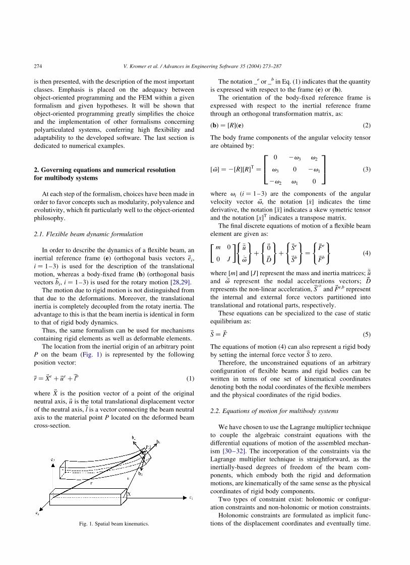
The location from the inertial origin of an arbitrary point

P on the beam (Fig. 1) is represented by the following

position vector:

~r ¼ ~Xe þ ~ue þ ~lb ð1Þ

where ~X is the position vector of a point of the original

neutral axis, ~u is the total translational displacement vector

of the neutral axis, ~l is a vector connecting the beam neutral

axis to the material point P located on the deformed beam

cross-section.

The notation _e or _b in Eq. (1) indicates that the quantity

is expressed with respect to the frame ðeÞ or ðbÞ:

The orientation of the body-fixed reference frame is

expressed with respect to the inertial reference frame

through an orthogonal transformation matrix, as:

ðbÞ ¼ ½R�ðeÞ ð2Þ

The body frame components of the angular velocity tensor

are obtained by:

~v½ � ¼ 2½ _R�½R�T ¼

0 2v3 v2

v3 0 2v1

2v2 v1 0

2664

3775 ð3Þ

where vi ði ¼ 1–3Þ are the components of the angular

velocity vector ~v; the notation ½_x� indicates the time

derivative, the notation ½~x� indicates a skew symetric tensor

and the notation ½x�T indicates a transpose matrix.

The final discrete equations of motion of a flexible beam

element are given as:

m 0

0 J

" #€~u

_~v

8<:

9=;þ

~0

~D

8<:

9=;þ

~Se

~Sb

8<:

9=; ¼

~Fe

~Fb

8<:

9=; ð4Þ

where ½m� and ½J� represent the mass and inertia matrices; €~u

and _~v represent the nodal accelerations vectors; ~D

represents the non-linear acceleration, ~Se;b

and ~Fe;b represent

the internal and external force vectors partitioned into

translational and rotational parts, respectively.

These equations can be specialized to the case of static

equilibrium as:

~S ¼ ~F ð5Þ

The equations of motion (4) can also represent a rigid body

by setting the internal force vector ~S to zero.

Therefore, the unconstrained equations of an arbitrary

configuration of flexible beams and rigid bodies can be

written in terms of one set of kinematical coordinates

denoting both the nodal coordinates of the flexible members

and the physical coordinates of the rigid bodies.

2.2. Equations of motion for multibody systems

We have chosen to use the Lagrange multiplier technique

to couple the algebraic constraint equations with the

differential equations of motion of the assembled mechan-

ism [30–32]. The incorporation of the constraints via the

Lagrange multiplier technique is straightforward, as the

inertially-based degrees of freedom of the beam com-

ponents, which embody both the rigid and deformation

motions, are kinematically of the same sense as the physical

coordinates of rigid body components.

Two types of constraint exist: holonomic or configur-

ation constraints and non-holonomic or motion constraints.

Holonomic constraints are formulated as implicit func-

tions of the displacement coordinates and eventually time.Fig. 1. Spatial beam kinematics.

V. Kromer et al. / Advances in Engineering Software 35 (2004) 273–287274

They express a restriction on the number of degrees of

freedom and therefore, on the set of possible configurations

of the system. A set of algebraic equations representing

holonomic constraint conditions between the displacement

coordinates is written as:

~QHð~d; tÞ ¼ ~0 ð6aÞ

›QH

›~d

" #{d~d} ¼ ½BH�{d~d} ¼ {~0} ð6bÞ

where

d~d ¼d~u

d ~a

( )

is the virtual generalized displacement vector, d ~a the virtual

rotation vector of the body-fixed basis.

Nonholonomic constraints conditions can only be

expressed as a relation between the differentials of the

coordinates and not as a finite relation between the

coordinates themselves. Constraints of this kind are such

that they cannot be integrated to be transformed to the

holonomic type. They bring a restriction on the behaviour of

the system, but not on the set of possible configurations. A

set of non-integrable equations concerning non-holonomic

constraints is written as:

~QNHð~d; ~_d; tÞ ¼ ~0 ð7aÞ

›QNH

›~_d

" #{d~_d} ¼ ½BNH�{d~_d} ¼ {~0} ð7bÞ

Another distinction is made between constraints involving

equalities, which are called bilateral constraints, and

constraints involving inequalities, named unilateral con-

straints. Holonomic constraints are only of the bilateral type.

Unilateral constraints are usually considered of the non-

holonomic type.

Given the constraints (6) and (7), the virtual work for the

unconstrained system is modified by the inclusion of the

virtual work which enforces the constraints through the

Lagrange multiplier technique. The equations of motion for

constrained flexible multibody systems are written as

follows:

m 0

0 J

" #{~€d} þ ½B�T ~l ¼

~Qu

~Qv

8<:

9=; ð8Þ

where

~€d ¼~€u

~_v

8<:

9=;

and ~l designates the vector of the Lagrange multipliers.

In order to alleviate the equations, the same notation has

been used (in Eq. (8) or in Eq. (4)) to represent elementary

or assembled matrices and vectors. The right-hand side

vector of Eq. (8) contains the remaining force-type terms as:

~Qu

~Qv

8<:

9=; ¼

~Fe

~Fb

8<:

9=;2

~Se

~Sb

8<:

9=;2

~0

~D

8<:

9=; ð9Þ

In Eq. (8), the notation contains both the holonomic and

non-holonomic constraints in the constraint force vector

½B�T ~l as:

½B� ¼BH

BNH

" #~l ¼

lH

lNH

( )ð10Þ

The ½B� matrix, called the matrix of constraints gradients

(or the constraint Jacobian matrix), is deduced from the

kinematic relationship between the bodies of the system.

These relationships can be imposed on the nodal degrees of

freedom of two separated flexible beams, or between a beam

nodal degree of freedom and a rigid body. Classical

Jacobian matrices modeling standard joints (universal,

revolute, spherical, translational joints) are described in

Ref. [33]. Specific joints (rigid or flexible wheel element)

describing contact conditions (with bi- or unilateral contact,

with or without friction and slipping) are described in

Ref. [34].

Thus, given the Jacobian matrices for the joints and beam

connections, the Eq. (8) can be employed in a systematic

manner to represent an arbitrary assemblage of articulated

flexible and rigid components.

2.3. Resolution of multibody systems equations

The resolution of multibody systems equations requires

the use of an adapted algorithm for the time integration of

the generalized coordinates. It must also include a proper

treatment of 3D finite rotations [35,36], as well as a

method to satisfy the kinematic constraints conditions. In

order to introduce an attractive modularity in the solution

procedures, which favors the object-oriented philosophy,

we have chosen to implement the staggered explicit-

implicit procedure proposed by Park [37]. The key to this

procedure is a staggered implementation of a separate

generalized coordinates integrator and constraints force

solver modules [37,38]. An explicit algorithm, described

in Section 2.3.1, is used to integrate the translational

displacements and the angular velocities of the system.

Once the angular velocities are obtained, the configuration

orientation is updated according to an implicit method

presented in Section 2.3.2. Finally, the Lagrange multi-

pliers are calculated in a separate routine, described in

Section 2.3.3, which implicitly integrates a stabilized

companion differential equation for the constraint forces

in time.

2.3.1. Integration of the generalized coordinates

Unconditional stability in time integration schemes can

be obtained with implicit algorithms, such as Newmark,

V. Kromer et al. / Advances in Engineering Software 35 (2004) 273–287 275

but increases the complexity of the computation scheme.

For this reason, the generalized coordinates are calculated

with a particular explicit integration procedure, called ‘two-

stage staggered algorithm’ [38]. The stability analysis of

this algorithm can be found in Ref. [39]. The algorithm is

based on an interlaced application of the central difference

algorithm such that the generalized coordinates are

advanced one-half time step at a time, as follows:

_~unþð1=2Þ ¼ _~un2ð1=2Þ þ h€~un ð11aÞ

~unþð1=2Þ ¼ ~un2ð1=2Þ þ h_~un ð11bÞ

~vnþð1=2Þ ¼ ~vn2ð1=2Þ þ h _~vn ð11cÞ

2.3.2. Updating of the rotational orientation

The rotational orientation parameters are not directly

integrable from the angular velocity vector. As a

consequence, a procedure must be developed to update

the configuration orientation given the angular velocity.

Various methods have been proposed for the parametriza-

tion of large rotations (Euler angles, Bryant angles,

rotational vector, Rodrigues parameters, Euler parameters).

An overview of these methods can be found in Refs. [34,

40]. The Euler parameters representation has been chosen

in this work, because of its algebraic nature and especially

because it does not possess any singularity limitation. As

such, Euler parameters appear to be the only set that allows

the treatment of rotations of arbitrary magnitude without

resorting to any special precautions [41]. Any finite

rotation can be uniquely represented with a rotation angle

u and a rotation axis ~n (Euler–Chasles theorem). The four

Euler parameters are defined as:

q0 ¼ cosu

2~q ¼ sin

u

2~n ð12Þ

and are subject to the constraint equation:

q20 þ ~qT

~q ¼ 1 ð13Þ

The rotation matrix is a function of the Euler parameters

as:

½R� ¼ ½I� þ 2q0½~q�T þ 2½~q�½~q� ð14Þ

Given (3) and (14), the angular velocity vector is expressed

in terms of the Euler parameters and their time

derivatives as:

0

~v

( )¼ 2

q0 ~qT

2~q q0½I�2 ½~q�

" #_q0

_~q

( )ð15Þ

By inverting (15), the Euler parameters derivatives are

obtained in terms of the body frame angular velocity

components:

_q0

_~q

( )¼

1

2

0 2 ~vT

~v ½ ~v�T

" #q0

~q

( )¼ ½Að ~vÞ�{q} ð16Þ

The configuration orientation is deduced from a time

discretization of (16). The Euler parameters derivatives are

subject to the following constraint conditions:

_q0q0 þ_~qT~q ¼ 0 ð17Þ

Among several possible schemes, the implicit trapezoidal

formula gives an approximation which satisfies (17) in the

discrete sense:

1

hð~qnþ1 2 ~qnÞ ¼ ½Að ~vnþð1=2ÞÞ�

1

2ð~qnþ1 þ ~qnÞ ð18Þ

where h is the time step.

The discrete orientation update is then given by:

~qnþ1 ¼1

D½I� þ

h

2½Að ~vnþ1=2Þ�

� �½I� þ

h

2½Að ~vnþ1=2Þ�

� �~qn

ð19Þ

where D ¼ 1 þ ðh2=4Þk ~vk2 and the notation k~xk designates

the Euclidian norm.

2.3.3. Lagrange multipliers treatment

The Lagrange multipliers are solved by the use of a

stabilized constraint force procedure. To effect a partitioned

solution of the constraints, we use the well-known penalty

technique, so that the constraint forces are made pro-

portional to violations of the constraint conditions:

~lH ¼1

1~QHð~d; tÞ ~lNH ¼

1

1~QNHð~d; tÞ ð20Þ

where 1 is a constant penalty coefficient ð0 , 1p 1Þ:

To solve ~l separately, the algebraic forms (20) must be

transformed into differential forms. First, equations (20) are

differentiated once as follows:

~_lH ¼1

1½BH�~_d ~_lNH ¼

1

1½BNH�~€d ð21Þ

Let us rewrite the equations of motion (8) as:

~€d ¼ ½M�21ð{Q} 2 ½B�T ~lÞ ð22Þ

where ½M� represents the mass and inertia matrix of (8).

For non-holonomic constraints, upon substituting (21)

into (22), one obtains the following stabilized differential

equation:

1~_lNH þ ½BNH�½M�21½BNH�T ~lNH ¼ ½BNH�½M�21{Q} ð23Þ

For holonomic constraints, the equations of motion (22) are

first integrated using the implicit forward Euler formula as:

_~dnþ1 ¼ h€~dnþ1 þ

_~dn ð24Þ


By substituting the result of the integration of (22) into

(21), we obtain the stabilized differential equation for

the Lagrange multipliers as:

1_~lHnþ1

þ h½BH�½M�21½BH�T ~lHnþ1

¼ h½BH�½M�21 ~Qnþ1 þ ½BH�_~dn ð25Þ

As one can see, the stabilized differential equation for

holonomic (25) or non-holonomic (23) constraints can be

written in the same form:

1_~lþ c1½B�½M�21½B�T ~l ¼ c1½B�½M�21 ~Qnþ1 þ c2½B�

_~dn ð26Þ

with c1 equal to h or 1 and c2 equal to 1 or 0, for holonomic

and non-holonomic constraints, respectively.

Finally, Eq. (26) is integrated by the forward Euler

formula; the discrete update of the Lagrange multipliers is

obtained as follows:

ð1½I� þ c1h½B�½M�21½B�T Þ ~lnþ1

¼ 1 ~ln þ c1h½B�½M�21 ~Qnþ1 þ c2h½B�_~dn ð27Þ

The accuracy and robustness of this staggered, stabilized

procedure for the solution of the constraints have been

established in Ref. [37].

As one can see, the updating of the generalized

coordinates, of the rotational orientation and of the

Lagrange multipliers are performed separately. For each

time step, the generalized coordinates are first calculated

and are used to update the right-hand side vector ~Q: This

vector is put into the Lagrange multiplier update module.

Finally, the right-hand side vector ~Q is corrected with the

current constraint force vector ½B�T ~l: The procedure is then

advanced to the next time step.

These separated treatments lead to an attractive modular

software implementation, which favors the object-oriented

philosophy and eases the introduction of new algorithms

and new formalisms in the future. Section 3 is dedicated to

the description of the object-oriented architecture of the

multibody analysis software.

3. Object-oriented design of the computational engine

3.1. Object-oriented concepts

Procedural languages like C, Pascal and Fortran

consider data as passive and memory occupying

elements, which can be manipulated only by functions

and procedures. In contrast, the object-oriented philos-

ophy comes from the idea that tools (methods) must be

associated with the information (data or attributes) they

manage. The key concepts of object-oriented program-

ming (abstraction, encapsulation, inheritance, polymorph-

ism) can be found in many computer journals and

language user guides [42–45]. Thus we will only present

briefly those concepts and try to show their similarities to

the structure of multibody systems.

The abstraction of the data type is realized by the

means of a class. A class incorporates the definition of

the structure as well as the operations on the abstract

data type. An object is an instance of the class, which

means that it is the material realisation of the abstract

data type defined by the class. For instance, at its highest

level of abstraction, the architecture of a multibody

system can be thought of as consisting of four basic

objects: bodies, constraints between bodies, loads and

motions.

The encapsulation designates the independent self-

containment of classes and their methods and attributes.

Encapsulation is an ideal concept for multibody systems, as

its implementation concentrates the attributes and methods

associated with an object such that access is permitted only

through well-defined interfaces. This full modularity greatly

enhances introducing modifications in the development

phase of the software, as well as performing on-going

maintenance.

The inheritance concept is used to define object

hierarchies. An object can have many children (instances

of a subclass) which inherit its data and member functions.

A subclass is usually of a special type and has additional

methods and attributes members relating to it. For example,

for multibody systems, the behavior and properties of

specific types of bodies (rigid, flexible, …), joints (revolute,

universal, spherical, prismatic, …), loads (punctual loads,

distributed loads, …) are specified and implemented in

classes derived from the base classes.

The last concept is polymorphism, which designates the

capability of object-oriented applications to interpret the

same request differently depending on the object being

processed. It is realised through the definition of abstract

objects using virtual member functions. Abstract objects

allow the writing of generic algorithms and the easy

extension of the existing code. For example, if Joint were

an abstract class, it could contain the definition of a virtual

method get_jacobian_matrix( ), which is in fact a dummy

method that does not actually do anything. All this definition

is simply to declare that Jacobian matrices can be obtained

from joints. The actual calculation of the jacobian matrices

is done within the descendants of class Joint. As a child of

Joint, Revolute_Joint is also able to give a jacobian matrix,

and the method get_jacobian_matrix( ) would contain the

code needed to actually perform its calculation. Similarly,

Spherical_Joint and Prismatic_Joint could be defined with

their methods for calculating Jacobian matrices. Thus,

through polymorphism, it is possible to describe any

constraint between two bodies without regard to joint type

and body type (rigid, flexible, etc). The implementation

details of the specific bodies and joints involved in

the connection are hidden by abstraction in the joint and

body objects.


3.2. Global description of the computational engine

Actual object-oriented programming still faces the

problem of choosing a language: it is obvious that the

code organization and even the algorithms used depend

heavily on this choice. Although Cþþ compilers obviously

do not optimize the code as much as Fortran compilers, we

selected Cþþ , which seems to be, currently, the language

providing numerical efficiency, portability, flexibility and is

easy to use [10].

As the complexity of the software increases, it becomes

necessary to employ good analysis tools. We decided to use

unified modeling language (UML) [46], which appears to be

the technique most commonly used. UML is a standardized

modeling language, with a set of symbols and rules

describing the relationships between the symbols.

In this paper, we will focus on the computational engine

of the software, for the treatment of three-dimensional

multibody flexible mechanisms with large rotations and

large strains [47,48]. It is written in Cþþ ANSI,

independently of the preprocessor, the postprocessor and

the compiler. The current architecture is based on the

hypotheses and formalism presented in the previous section.

However, it has been conceived to provide a flexible and

extensive set of objects that facilitate multibody systems

analysis and which can be adapted to meet future

developments.

The global architecture is organized around several basic

classes associated with the classical steps of a multibody

finite element analysis (geometry definition, meshing,

interactions definition, finite element formulation, beha-

viour law, joints definition, solving algorithms, writing

results). The description of these classes is presented in

Section 3.3.

The management of the different stages of the analysis is

performed by the major class Domain, which represents the

heart of the software architecture (Fig. 2). It has been

created to represent an elementary problem (corresponding

to a specific multibody system analysis). The complete

description of the class Domain is given in Section 3.4.

3.3. Description of the basic classes

3.3.1. Common tools

Some utility classes have been developed to manage

mathematical tools, variable size of objects, stacks, buffers,

pools for memory management, read and write protection

on objects and execution time measurement, among others

(for example, classes Vect, TabVect, Matrix, SMatrix,

DMatrix, List). The implementation of these classes is

based on the templates mechanism, which allows the

definition of the concepts (methods, algorithms) indepen-

dently of the type of object being used.

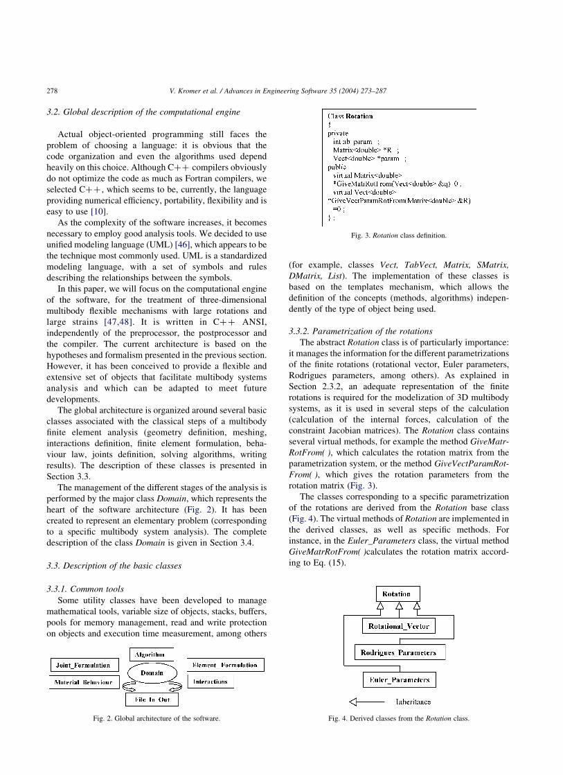
3.3.2. Parametrization of the rotations

The abstract Rotation class is of particularly importance:

it manages the information for the different parametrizations

of the finite rotations (rotational vector, Euler parameters,

Rodrigues parameters, among others). As explained in

Section 2.3.2, an adequate representation of the finite

rotations is required for the modelization of 3D multibody

systems, as it is used in several steps of the calculation

(calculation of the internal forces, calculation of the

constraint Jacobian matrices). The Rotation class contains

several virtual methods, for example the method GiveMatr-

RotFrom( ), which calculates the rotation matrix from the

parametrization system, or the method GiveVectParamRot-

From( ), which gives the rotation parameters from the

rotation matrix (Fig. 3).

The classes corresponding to a specific parametrization

of the rotations are derived from the Rotation base class

(Fig. 4). The virtual methods of Rotation are implemented in

the derived classes, as well as specific methods. For

instance, in the Euler_Parameters class, the virtual method

GiveMatrRotFrom( )calculates the rotation matrix accord-

ing to Eq. (15).

Fig. 4. Derived classes from the Rotation class.

Fig. 3. Rotation class definition.

Fig. 2. Global architecture of the software.


3.3.3. Finite element formulation

Element and Node are traditional classes used for the

representation of finite elements. The class Element_For-

mulation (Fig. 5) is the abstract master class of the finite

elements library. It provides virtual methods of computation

of the different finite element arrays and tables (Fig. 6) (as,

for example, the classical mass and rigidity matrices, the

strain increments vector, the non-linear acceleration vector,

the internal forces vector). The effective computation

depends on the chosen formalism and may vary appreciably.

In these conditions, the object-oriented philosophy eases the

implementation of new formalisms, without requiring a

complete redefinition of the software’s architecture.

The abstract class Element_Type contains virtual

methods for the calculation of the element’s shape function

and its derivatives. It possesses an attribute which is a

pointer to an Element object. From Element_Type, sub-

classes corresponding to a specific finite element are derived

(for example, Beam2 for a two-nodes beam element).

The class Beam2_Formulation is derived from Ele-

ment_Formulation. One of its attributes is a pointer to the

desired finite element, Beam2, for example. This class

corresponds to a specific finite element formulation, and

allows the redefinition of the methods according to the type

of the element. For instance, the formalism implemented in

the current code requires the calculation of curvatures and

curvature increments of the beams. As a consequence,

besides the methods already defined in its mother class

Element_Formulation, the class Beam2_Formulation also

contains specific methods such as Calculate_Curvatures( ),

Calculate_Curvature_Increments( ) (Fig. 7).

3.3.4. Behaviour law

In most object-oriented calculation software, the material

behaviour is included in the finite element formulation. In

our code architecture, a separated class Material_Behaviour

has been created, which contains the virtual methods for the

calculation of the stresses according to a given material

behaviour law (Fig. 5). The current formalism introduces a

rate-type constitutive law that relates the instantaneous rate

of stress to the instantaneous rate of deformation. The

methods for a linear elastic material are defined in the

derived class Linear_Elastic_Behaviour (for example, the

methods Calc_tgt_oper(), Calc_str_inc(), Calc_res_

str_inc() calculate the tangent operator, the stress incre-

ments and the resultant stress increments, respectively).

Fig. 6. Element_Formulation class definition.

Fig. 5. Classes associated with the finite element modelization and with material behaviour.


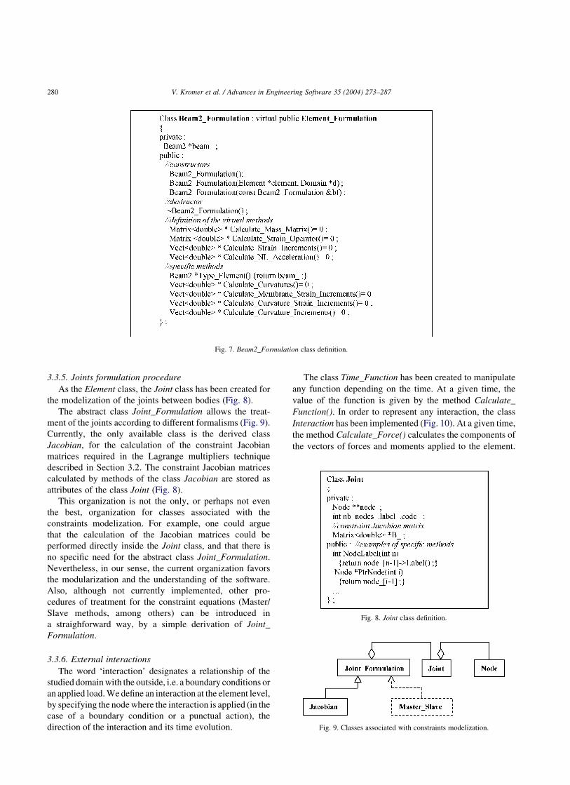
3.3.5. Joints formulation procedure

As the Element class, the Joint class has been created for

the modelization of the joints between bodies (Fig. 8).

The abstract class Joint_Formulation allows the treat-

ment of the joints according to different formalisms (Fig. 9).

Currently, the only available class is the derived class

Jacobian, for the calculation of the constraint Jacobian

matrices required in the Lagrange multipliers technique

described in Section 3.2. The constraint Jacobian matrices

calculated by methods of the class Jacobian are stored as

attributes of the class Joint (Fig. 8).

This organization is not the only, or perhaps not even

the best, organization for classes associated with the

constraints modelization. For example, one could argue

that the calculation of the Jacobian matrices could be

performed directly inside the Joint class, and that there is

no specific need for the abstract class Joint_Formulation.

Nevertheless, in our sense, the current organization favors

the modularization and the understanding of the software.

Also, although not currently implemented, other pro-

cedures of treatment for the constraint equations (Master/

Slave methods, among others) can be introduced in

a straighforward way, by a simple derivation of Joint_

Formulation.

3.3.6. External interactions

The word ‘interaction’ designates a relationship of the

studied domain with the outside, i.e. a boundary conditions or

an applied load. We define an interaction at the element level,

by specifying the node where the interaction is applied (in the

case of a boundary condition or a punctual action), the

direction of the interaction and its time evolution.

The class Time_Function has been created to manipulate

any function depending on the time. At a given time, the

value of the function is given by the method Calculate_

Function(). In order to represent any interaction, the class

Interaction has been implemented (Fig. 10). At a given time,

the method Calculate_Force() calculates the components of

the vectors of forces and moments applied to the element.

Fig. 9. Classes associated with constraints modelization.

Fig. 7. Beam2_Formulation class definition.

Fig. 8. Joint class definition.


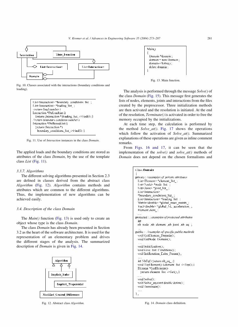
The applied loads and the boundary conditions are stored as

attributes of the class Domain, by the use of the template

class List (Fig. 11).

3.3.7. Algorithms

The different solving algorithms presented in Section 2.3

are defined in classes derived from the abstract class

Algorithm (Fig. 12). Algorithm contains methods and

attributes which are common to the different algorithms.

Thus, the implementation of new algorithms can be

achieved easily.

3.4. Description of the class Domain

The Main() function (Fig. 13) is used only to create an

object whose type is the class Domain.

The class Domain has already been presented in Section

3.2 as the heart of the software architecture. It is used for the

representation of an elementary problem and drives

the different stages of the analysis. The summarized

description of Domain is given in Fig. 14.

The analysis is performed through the message Solve() of

the class Domain (Fig. 15). This message first generates the

lists of nodes, elements, joints and interactions from the files

created by the preprocessor. Three initialization methods

are then activated and the resolution is initiated. At the end

of the resolution, Terminate() is activated in order to free the

memory occupied by the initializations.

At each time step, the calculation is performed by

the method Solve_at(). Fig. 17 shows the operations

which follow the activation of Solve_at(). Summarized

explanations of these operations are given as inline comment

remarks.

From Figs. 16 and 17, it can be seen that the

implementation of the solve() and solve_at() methods of

Domain does not depend on the chosen formalisms and

Fig. 10. Classes associated with the interactions (boundary conditions and

loading).

Fig. 11. Use of Interaction instances in the class Domain.

Fig. 13. Main function.

Fig. 12. Abstract class Algorithm. Fig. 14. Domain class definition.


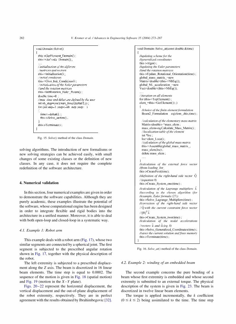
solving algorithms. The introduction of new formalisms or

new solving strategies can be achieved easily, with small

changes of some existing classes or the definition of new

classes. In any case, it does not require the complete

redefinition of the software architecture.

4. Numerical validation

In this section, four numerical examples are given in order

to demonstrate the software capabilities. Although they are

purely academic, these examples illustrate the potential of

the software, whose computational engine has been designed

in order to integrate flexible and rigid bodies into the

architecture in a unified manner. Moreover, it is able to deal

with both open-loop and closed-loop in a systematic way.

4.1. Example 1: Robot arm

This example deals with a robot arm (Fig. 17), whose two

similar segments are connected by a spherical joint. The first

segment is subjected to the prescribed angular rotation

shown in Fig. 17, together with the physical description of

the robot.

The left extremity is subjected to a prescribed displace-

ment along the Z axis. The beam is discretized in 16 linear

beam elements. The time step is equal to 0.0002. The

sequence of the motion is given in Fig. 18 (spatial motion)

and Fig. 19 (motion in the X –Y plane).

Figs. 20–22 represent the horizontal displacement, the

vertical displacement and the out-of-plane displacement of

the robot extremity, respectively. They are in perfect

agreement with the results obtained by Ibrahimbegovic [32].

4.2. Example 2: winding of an embedded beam

The second example concerns the pure bending of a

beam whose first extremity is embedded and whose second

extremity is submitted to an external torque. The physical

description of the system is given in Fig. 23. The beam is

discretized in twelve linear beam elements.

The torque is applied incrementally, the k coefficient

ð0 # k # 2Þ being assimilated to the time. The time step

Fig. 16. Solve_at() method of the class Domain.

Fig. 15. Solve() method of the class Domain.


Fig. 19. Motion of the robot arm in the X –Y plane.

Fig. 20. Horizontal displacement of the robot extremity.

Fig. 21. Vertical displacement of the robot extremity.

Fig. 22. Out-of-plane displacement of the robot extremity.

Fig. 23. Pure bending of an embedded beam: problem data.

Fig. 24. Successive deflections of the embedded beam.

Fig. 17. Robot arm: problem data.

Fig. 18. Spatial motion of the robot arm.

Fig. 25. Evolution of the angle u versus u=L:

Fig. 26. Evolution of the angle u versus v=L:


is equal to Dk ¼ 0; 0002: The successive deflections are

shown in Fig. 24.

According to the Euler classical formula [49], the

deflection of the beam is a circle portion, the analytical

expressions of the horizontal and vertical displacements of

the extremity supporting the torque are given by:

u ¼ L 2L

u=2sin

u

2

� �cos

u

2

� �v ¼

L

u=2sin2 u

2

� �

w ¼ 0

ð28Þ

with

u ¼ML

EIð29Þ

With Figs. 25 and 26, it is possible to compare the evolution

of the angle u versus u=L and v=L; respectively, for both the

numerical and the analytical solutions.

For u ¼ 2p; the deformed configuration of the beam is a

closed circle. With Table 1, it is also possible to compare

our results with the analytical solution and with the results

obtained by Surana et al. [49], respectively. It can be seen

that the results are in good agreement.

4.3. Example 3: three-bar mechanism

The third example is a three-bar mechanism (Fig. 27).

The bars 1 and 3 are rigid. They are connected through

revolution joints to the flexible bar 2. Densities and

inertia are the same for the three bars. The first bar is

submitted to a constant angular velocity v:

The rigid bars are discretized in two linear beam

elements, while the flexible bar is discretized in four

linear beam elements.

The time step is equal to 0.0002. The successive

deflections are shown in Fig. 28.

The vertical and horizontal displacements of joint 1 are

represented in Figs. 29 and 30. They are in perfect


Table 1

Comparison of the evolution of the horizontal and vertical displacements ðu; vÞ of the extremity

k ðu; vÞ Analytical solution ðu; vÞ Surana et al. [49] Relative error (%) ðu; vÞ Current solution Relative error (%)

0.2 (20.774; 3.648) (20.765; 3.623) (1.16; 0.68) (20.605; 3.220) (21.84; 11.73)

0.4 (22.918; 6.598) (22.899; 6.574) (0.65; 0.36) (22.803; 6.521) (3.94; 1.16)

0.6 (25.945; 8.333) (25.955; 8.328) (0.17; 0.06) (26.234; 8.522) (4.86; 2.27)

0.8 (29.194; 8.637) (29.293; 8.620) (1.07; 0.20) (28.889; 8.712) (3.31; 0.86)

1.0 (212.000; 7.639) (212.215; 7.507) (1.80; 1.70) (212.005; 7.768) (0.04; 1.69)

1.2 (213.870; 5.758) (214.120; 5.376) (1.80; 6.63) (213.809; 6.043) (0.43; 4.95)

1.4 (214.590; 3.571) (214.660; 2.877) (0.48; 19.43) (214.859; 3.428) (1.84; 4.00)

1.6 (214.270; 1.650) (213.850; 0.797) (2.94; 51.7) (214.478; 1.427) (1.46; 13.51)

1.8 (213.250; 0.405) (212.180; 20.123) (8.07; 130.0) (213.300; 0.390) (0.38; 3.77)

Fig. 27. Three-bar mechanism: problem data.

Fig. 28. Successive deformed configurations of the three-bar mechanism.

Fig. 29. Evolution of the horizontal displacement of joint 1.


4.4. Example 4: helical motion of a pinned beam

The pinned beam presented in Fig. 31 is subjected to

slide along the Z axis, under a constant torque and a constant

concentrated force applied to the pinned extremity. The

physical description of the beam is given in Fig. 31. The

beam is discretized in ten linear beam elements. The timestep is equal to 0.0002. The sequence of the motion is given

in Fig. 32.

Figs. 33–35 represent the horizontal displacement, the

vertical displacement and the out-of-plane displacement of

the free extremity, respectively. They are in perfect


5. Conclusions

A finite element calculation software may advance in

different directions. In particular, for software dealing with

multibody systems, many formalisms and hypotheses can

evolve and combine with each other, as for example,

the choice of the finite elements, the choice of the referential

frame, the definition of physical or material parameters, the

choice of the parameters for the representation of the finite

rotations, the choice of the solving algorithm, the formalism

and the treatment of the joints, the flexibility or the rigidity

of the bodies, among others.

Fig. 31. Helical motion of a pinned beam: problem data.

Fig. 32. Spatial motion of the pinned beam.

Fig. 33. Horizontal displacement of the free extremity.

Fig. 34. Vertical displacement of the free extremity.

Fig. 35. Out-of-plane displacement of the free extremity.

Fig. 30. Evolution of the vertical displacement of joint 1.


In this paper, the architecture of a new finite element

software for the simulation of flexible mechanisms has been

presented. The program has been designed according to

object-oriented principles. This approach allows us to

simplify the architecture of the program and to take

advantage of the inherent synergy between object-oriented

design and multibody systems analysis. Additional benefits,

such as improved maintainability, flexibility and ease of

expansion, also accrue as a result. The flexibility of the

software is made possible by the clear modularization that

can be reached with object-oriented programming, with a

marked separation of functionalities. Extensibility and

reusability of object-oriented programming are clearly

shown: the introduction of new formalisms or new solving

strategies can be achieved easily, with small changes of

some existing classes or the definition of new classes. In any

case, it does not require the complete redefinition of the

software architecture.

References

[1] Miller GR. A LISP-based object-oriented approach to structural

analysis. Engng Comput 1988;4:197–203.

[2] Foerch R. Un environnement oriente objet pour la modelisation

numerique des materiaux en calcul des structures. Thesis. Ecole

Nationale Superieure des Mines de Paris; 1996.

[3] Besson J, Leriche R, Foerch R, Cailletaud G. Object-oriented

programming applied to the finite element method. Part II.

Application to material behaviors. Revue Europeenne des elements

Finis 1998;7(5):567–88.

[4] Hsieh SH, Sotelino ED. A message-passing class library Cþþ for

portable parallel programming. Engng Comput 1997;13:20–34.

[5] Breitkopf P, Escaig Y. Object-oriented approach and distributed finite

element simulations. Revue Europeenne des Elements Finis 1998;

7(5): 609–26.

[6] Potapov S, Jacquart G. Un algorithme ALE de dynamique rapide base

sur une approche mixte elements finis-volumes finis. Proceedings of

3eme Colloque National en calcul des structures de Giens; 1997. p.

509–14.

[7] Gelin JC, Walterthum L. Conception d’un logiciel oriente-objets pour

la simulation de processus de formage. Proceedings of 2eme Colloque

National en calcul des structures de Giens; 1995. p. 552–8.

[8] Walterthum L. Programmation orientee objet et calcul par elements

finis. Application a la conception d’un logiciel de simulation en mise

en forme des materiaux. Thesis. Universite de Franche-Comte; 1996.

[9] Gelin JC, Paquier P, Walterthum L. Application de la POO pour la

conception d’un logiciel de simulation par elements finis en mise en

forme des materiaux. Revue Europeenne des Elements Finis 1998;

7(5):505–33.

[10] Klapka I, Cardona A, Geradin M. An object oriented implementation

of the finite element method for coupled problems. Revue Europeenne

des Elements Finis 1998;7(5):469–504.

[11] Dubois-Pelerin Y, Pegon P. Object-oriented programming in non-

linear finite element analysis. Comput Struct 1998;67:225–41.

[12] Eyheramendy D, Zimmermann T. Programmation orientee objet

appliquee a la methode des elements finis: derivations symboliques,

programmation automatique. Revue Europeenne des Elements Finis

1995;4:327–60.

[13] Eyheramendy D. An object-oriented hybrid symbolic/numerical

approach for the development of finite element codes. Finite Elem

Anal Des 2000;36:315–34.

[14] Eyheramendy D, Zimmermann T. Integration d’une approche

variationnelle pour la methode des elements finis dans un environne-

ment oriente objet. Revue Europeenne des Elements Finis 1998;7(5):

589–607.

[15] Mackie RI. Object-oriented programming and numerical methods.

Microcomput Civil Engng 1991;6:123–8.

[16] Scholz SP. Elements of an object-oriented FEMþþ program in

Cþþ . Comput Struct 1992;43(3):517–29.

[17] Remy P, Devloo B, Alves Filho JSR. An object-oriented approach to

finite element programming (phase I): a system independent window-

ing environment for developing interactive scientific programs. Adv

Engng Software 1992;14:41–6.

[18] Besson J, Foerch R. Object-oriented programming applied to the finite

element method. Part I. General concepts. Revue Europeenne des

Elements Finis 1998;7(5):535–66.

[19] Debordes O. Calcul des structures et architectures de logiciels.

Proceedings of 4eme Congres en Calcul des Structures de Giens;

1999. p. 61–78.

[20] Breitkopf P. Demarche objet et modelisation numerique. Proceedings

of 4eme Congres en Calcul des Structures de Giens; 1999. p. 79–84.

[21] Szewczyk ZP, Sleight DW. Object-oriented approach to interactive

analysis of structures. Adv Engng Software 2000;31:733–42.

[22] Pantale O. An object-oriented programming of an explicit dynamics

code: application to impact simulation. Adv Engng Software 2002;33:

297–306.

[23] Ryan RR. ADAMS: multibody system analysis software. In: Scheihlen

W, editor. Multibody systems handbook. Berlin: Springer; 1990.

[24] Nikravesh PE, Chung IS. Application of Euler parameters for the

dynamic analysis of three-dimensional constrained mechanical

systems. J Mech Des 1982;104:785–91.

[25] Nikravesh PE, Gim G. Systematic construction of the equations

of motion for multibody systems containing closed kinematic

loops. Proceedings of the ASME Design Automation Conference;

1989.

[26] Kunz DL. An object-oriented approach to multibody systems analysis.

Comput Struct 1998;69:209–17.

[27] Tisell C, Orsborn K. A system for multibody analysis based on object-

relational database technology. Adv Engng Software 2000;31:

971–84.

[28] Park KC, Downer JD, Chiou JC, Farhat C. A modular multibody

analysis capability for high precision, active control and real-time

applications. Int J Numer Meth Engng 1991;32:1767–98.

[29] Downer JD, Park KC, Chiou JC. Dynamics of flexible beams for

multibody systems: a computational procedure. Comput Meth Appl

Mech Engng 1992;96:373–408.

[30] Usoro PB, Nadira R, Mahil SS. A finite element/Lagrange approach to

modeling lightweight flexible manipulators. Trans ASME 1986;108:

198–205.

[31] Cardona A, Geradin M, Doan DB. Rigid and flexible joint modelling

in multibody dynamics using finite elements. Comput Meth Appl

Mech Engng 1991;89:395–418.

[32] Ibrahimbegovic A, Mamouri S. On rigid components and joint

constraints in nonlinear dynamics of flexible multibody systems

employing 3D geometrically exact beam model. Comput Meth Appl

Mech Engng 2000;188:805–31.

[33] Chiou JC. Constraint treatment techniques and parallel algorithms for

multibody dynamic analysis. PhD Thesis. University of Colorado; 1990.

[34] Cardona A. An integrated approach to mechanism analysis. PhD

Thesis. University of Liege; 1989.

[35] Ibrahimbegovic A. On the choice of finite rotation parameters.

Comput Meth Appl Mech Engng 1997;149:49–71.

[36] Ibrahimbegovic A, Mikdad M. Finite rotations in dynamics of beams

and implicit time-stepping schemes. Int J Numer Meth Engng 1998;

41:781–814.

[37] Park KC, Chiou JC. Stabilization of computational procedures for

constrained dynamical systems. J Guidance, Control Dyn 1988;11:

365–70.


[38] Park KC, Chiou JC, Downer JD. Explicit-Implicit staggered

procedure for multibody dynamics analysis. J Guidance, Control

Dyn 1990;13:562–70.

[39] Downer JD. A computational procedure for the dynamics of flexible

beams within multibody systems. PhD Thesis. University of Color-

ado; 1990.

[40] Cardona A, Geradin M. A beam finite element non-linear theory with

finite rotations. Int J Numer Meth Engng 1988;26:2403–38.

[41] Spring KW. Euler parameters and the use of quaternion algebra in the

manipulation of finite rotations: a review. Mech Mach Theory 1986;

21:365–73.

[42] Meyer B. Object-oriented software design. New Jersey: Prentice-Hall;

1988. ISBN: 0-13-629049-3 or 0-13-629031-0 PBK.

[43] Cox BJ. Object-oriented programming: an evolutionary

approach. Reading, MA: Addison-Wesley; 1986. ISBN: 0-201-

10393-1.

[44] Fenves GL. Object-oriented programming for engineering software

development. Engng Comput 1990;6:1–15.

[45] Miller GR. An object-oriented approach to structural analysis and

design. Comput Struct 1991;40(1):75–82.

[46] Rumbauch J, Jacobson I, Booch G. The unified modeling language

reference manual. Reading, MA: Addison-Wesley; 1999.

[47] Dufosse F. Approche orientee objet appliquee a la conception d’un

logiciel dedie a l’analyse des systemes multicorps. Thesis. Universite

Henri Poincare, Nancy I; 2001.

[48] Dufosse F, Kromer V, Mikolajczak A, Gueury M. Simulation of 3D

polyarticulated mechanisms through object-oriented approach. In:

Mastorakis N, editor. Problems in modern applied mathematics,

mathematics and computers in science and engineering. 2000. p. 84–9.

[49] Surana KS, Sorem RM. Geometrically non-linear formulation for

three dimensional curved beam elements with large rotations. Int J

Numer Meth Engng 1989;28:43–73.


Documents

An object-oriented design of a finite element code: application to multibody systems analysis