Embed Size (px)
Citation preview
An Introduction to Topological Insulators
Michel Fruchart, David Carpentier
To cite this version:
Michel Fruchart, David Carpentier. An Introduction to Topological Insulators. Comptes rendusde l’Academie des sciences. Serie IV, Physique, astrophysique, Elsevier, 2013, 14 (9), pp.779-815. <10.1016/j.crhy.2013.09.013>. <ensl-00868307v2>
HAL Id: ensl-00868307
https://hal-ens-lyon.archives-ouvertes.fr/ensl-00868307v2
Submitted on 3 Nov 2013
HAL is a multi-disciplinary open accessarchive for the deposit and dissemination of sci-entific research documents, whether they are pub-lished or not. The documents may come fromteaching and research institutions in France orabroad, or from public or private research centers.
L’archive ouverte pluridisciplinaire HAL, estdestinee au depot et a la diffusion de documentsscientifiques de niveau recherche, publies ou non,emanant des etablissements d’enseignement et derecherche francais ou etrangers, des laboratoirespublics ou prives.
Topological insulators/Isolants topologiques
An introduction to topological insulatorsIntroduction aux isolants topologiques
Michel Frucharta, David Carpentiera
aLaboratoire de physique, École normale supérieure de Lyon (UMR CNRS 5672), 46, allée d’Italie, 69007 Lyon, France
Abstract
Electronic bands in crystals are described by an ensemble of Bloch wave functions indexed by momenta defined inthe first Brillouin Zone, and their associated energies. In an insulator, an energy gap around the chemical potentialseparates valence bands from conduction bands. The ensemble of valence bands is then a well defined object,which can possess non-trivial or twisted topological properties. In the case of a twisted topology, the insulatoris called a topological insulator. We introduce this notion of topological order in insulators as an obstruction todefine the Bloch wave functions over the whole Brillouin Zone using a single phase convention. Several simplehistorical models displaying a topological order in dimension two are considered. Various expressions of thecorresponding topological index are finally discussed.
Résumé
Les bandes électroniques dans un cristal sont définies par un ensemble de fonctions d’onde de Bloch dépendant dumoment défini dans la première zone de Brillouin, ainsi que des énergies associées. Dans un isolant, les bandes devalence sont séparées des bandes de conduction par un gap en énergie. L’ensemble des bandes de valence est alorsun objet bien défini, qui peut en particulier posséder une topologie non triviale. Lorsque cela se produit, l’isolantcorrespondant est appelé isolant topologique. Nous introduisons cette notion d’ordre topologique d’une bandecomme une obstruction à la définition des fonctions d’ondes de Bloch à l’aide d’une convention de phase unique.Plusieurs modèles simples d’isolants topologiques en dimension deux sont considérés. Différentes expressions desindices topologiques correspondants sont finalement discutées.
Keywords: topological insulator, topological band theory, quantum anomalous Hall effect, quantum spin Halleffect, Chern insulator, Kane–Mele insulator
Mots-clés : isolant topologique, théorie des bandes topologique, effet Hall quantique anomal, effet Hallquantique de spin, isolant de Chern, isolant de Kane–Mele
1. Introduction
Topological insulators are phases of matter characterized by an order of a new kind, which is not fit into thestandard symmetry breaking paradigm. Instead these new phases are described by a global quantity which doesnot depend on the details of the system - a so-called topological order. More precisely, their ensemble of valencebands possess a non-standard topological property. A band insulator is a material which has a well-defined set ofvalence bands separated by an energy gap from a well-defined set of conduction bands. The object of interest inthe study of topological order in insulators is the ensemble of valence bands, which is unambiguously well definedfor an insulator. The question underlying the topological classification of insulators is whether all insulating phases
Email addresses: [email protected] (Michel Fruchart), [email protected] (David Carpentier)
Preprint submitted to CR Physique November 3, 2013
are equivalent to each other, i.e. whether their ensemble of valence bands can be continuously transformed intoeach other without closing the gap. Topological insulators correspond to insulating materials whose valence bandspossess non-standard topological properties. Related to their classification is the determination of topologicalindices which will differentiate standard insulators from the different types of topological insulators. A canonicalexample of such a topological index is the Euler–Poincaré characteristic of a two-dimensional manifold [1]. Thisindex counts the number of « holes » in the manifold. Two manifolds with the same Euler characteristic can becontinuously deformed into each other, which is not possible for manifolds with different Euler characteristics.
The existence of topological order in an insulator induces unique characteristic experimental signatures. Themost universal and remarkable consequence of a nontrivial bulk topology is the existence of gapless edge orsurface states; in other words, the surface of the topological insulator is necessarily metallic. An informal argumentexplaining those surface states is as follows. The vacuum as well as most conventional insulating crystals aretopologically trivial. At the interface between such a standard insulator and a topological insulator, it is notpossible for the « band structure » to interpolate continuously between a topological insulator and the vacuumwithout closing the gap. This forces the gap to close at this interface leading to metallic states of topologicalorigin.
This kind of topological phase ordering first arose in condensed matter in the context of the integer quantumHall effect. This phase, discovered in 1980 by Klaus von Klitzing et al. [2], is reached when electrons trappedin a two-dimensional interface between semi-conductors are submitted to a strong transverse magnetic field.Quantized plateaux appear for the Hall conductivity while the longitudinal resistance simultaneously vanishes[3]. In the bulk of the sample, the electronic states are distributed in Landau levels with a large gap betweenthem. The quantization of the Hall conductivity can be attributed within standard linear response theory to atopological property of these bulk Landau levels, the so-called first Chern number of the bands located below thechemical potential [4]. From this point of view the robustness of the phase manifested in the high precision ofthe Hall conductivity plateau is an expression of the topological nature of the related order, which by definitionis insensitive to perturbations. The existence of robust edge states is another manifestation of this topologicalordering. The quantized Hall conductivity can be alternatively accounted for by the ballistic transport propertiesof the edge states.
Note that in the initial work of Thouless et al. [4], this topological ordering was described as a propertyof electronic Bloch bands of electrons on a lattice, and was only generalized later to free electrons on a planarinterface. The topological property of the ensemble of Bloch states of a valence band can be inferred by theexplicit determination of these Bloch states. In a non-trivial or twisted insulator, one faces an impossibility orobstruction to define electronic Bloch states over the whole band using a single phase convention: at least twodifferent phase conventions are required, as opposed to the usual case. This obstruction is a direct manifestationof the non-trivial topology or twist of the corresponding band. It was realized in 1988 by D. Haldane [5] thatwhile this type of order was specific to two dimensional insulators, it did not require a strong magnetic field,but only time reversal symmetry breaking. This author considered a model of electrons on a bipartite lattice(graphene), with time-reversal symmetry broken explicitly but without any net magnetic flux through the lattice.The phase diagram consists then of three insulating phases, i.e. with a finite gap separating the conduction fromthe valence bands. These insulators only differs by their topological property, quantized by a Chern number. Theanalogous phases of matter are now denoted Chern topological insulators, or anomalous quantum Hall effect.Such a phase was recently discovered experimentally [6].
Within the field of topological characterization of insulators a breakthrough occurred with the seminal workof C. Kane and G. Mele [7, 8]. These authors considered the effect of a strong spin–orbit interaction on electronicbands of graphene. They discovered that in such a two dimensional system where the spin of electrons cannot beneglected in determining the band structure, the constraints imposed by time-reversal symmetry could lead to anew topological order and associated metallic edge states of a new kind. While the quantum Hall effect arisesin electronic system without any symmetry and is characterized by a Chern number, this new topological phaseis possible only in presence of time-reversal symmetry, and is characterized by a new Z2 index. It was called aquantum spin Hall phase. This discovery triggered a huge number of theoretical and experimental works on thetopological properties of time reversal symmetric spin-dependent valence bands and the associated surface statesand physical signatures. Soon after the initial Kane and Mele papers, A. Bernevig, T. Hughes and S.C. Zhangproposed a realistic realization of this phase in HgTe quantum wells [9]. They identified a possible mechanism
2
for the appearance of this Z2 topological order through the inversion of order of bulk bands around one pointin the Brillouin zone. This phase was discovered experimentally in the group of L. Molenkamp who conductedtwo-terminal and multi-probe transport experiments to demonstrate the existence of the edge states associatedwith the Z2 order [10, 11].
In 2007, three theoretical groups extended the expression of the Z2 topological index to three dimensions: itwas then realized that three dimensional insulating materials and not only quasi-two dimensional systems coulddisplay a topological order [12, 13, 14]. Several classes of materials, including the Bismuth compounds BiSb,Bi2Se3 and Bi2Te3, and strained HgTe were discovered to be three-dimensional topological insulators [15, 16, 17].The hallmark of the Z2 topological order in d = 3 is the existence of surface states with a linear dispersion andobeying the Dirac equation. The unique existence of these Dirac states as well as their associated spin polarizationspinning around the Dirac point have been probed by experimental surface techniques including Angle-ResolvedPhotoEmission (ARPES) and Scanning Tunneling Microscopy (STM). Their presence in several materials has beenconfirmed by numerous studies, while a clear signature of their existence on transport experiments has proven tobe more difficult to obtain. Note that such Dirac dispersion relations for topological surface states arise around asingle (or an odd number of) Dirac points in the Brillouin zone, as opposed to real two dimensional materials likegraphene where these Dirac points can only occur in pairs.
The purpose of the present paper is to introduce pedagogically the notion of topological order in insulators asa bulk property, i.e. as a property of the ensemble of Bloch wave functions of the valence bands. For the sake ofclarity we will discuss simple examples in dimension d = 2 only, instead of focusing on generals definitions. As aconsequence of this pedagogical choice, we will omit a discussion of the physical consequences of this topologicalorder, most notably the physical properties of Dirac surface states of interest experimentally, as well as otherkind topological order in, e.g., superconductors. The reader interested by these aspects can turn towards existingreviews [15, 16, 17, 18]. Note that a different notion of topological order was introduced in e.g. [19], whichdiffers from the property of topological insulators discussed in this review.
In the part which follows, we will define more precisely the object of study. In a following part (section 3), wewill describe the simplest model of a Chern insulator, i.e. in a two-bands system. This will give us an excuse todefine the Berry curvature and the Chern number, and to comprehend the nontrivial topology as an “obstruction”to properly define electronic wavefunctions. As the understanding of the more recent and subtle Z2 topologicalorder was carved by its discoverers in a strong analogy with the Chern topological order, these concepts will equipus for the third part (section 4), where we will develop simple models to understand the Z2 insulators as well asthe different expressions of the Z2 invariant characterizing them.
2. Bloch bundles and topology
The aim of this first part is to define more precisely the object of this paper, namely the notion of topologicalorder of an ensemble of valence bands in an insulator. We will first review a very simple example of nontrivialbundle: the Möbius strip, before defining the notion of valence Bloch bundle in an insulator.
2.1. The simplest twisted bundle: a Möbius strip
A vector bundle π : E → B is specified by a projection π from the bundle space E to the base space B. Thefiber Fx = π−1(x) above each point of the base x ∈ B is assumed to be isomorphic to a fixed typical fiber F . Thefibers Fx and F possesses a vector space structure assumed to be preserved by the isomorphism Fx
∼= F . Hence,the vector bundle E indeed looks locally like the cartesian product B× F . The bundle is called trivial if this alsoholds globally, i.e. E and B× F are isomorphic. When it is not the case, the vector bundle is said to be nontrivial,or twisted (see [20, 1] for details). As a consequence, a n-dimensional vector bundle is trivial iff it has a basis ofnever-vanishing global sections i.e. iff it has a set of n global sections which at each point form a basis of thefiber [21]. On the contrary, the obstruction to define a basis of never-vanishing global sections (or basis of thefibers) will signal a twisted topology of a vector bundle. In the following, we will rely on this property to identifya non-trivial topology of a vector bundle when studying simple models.
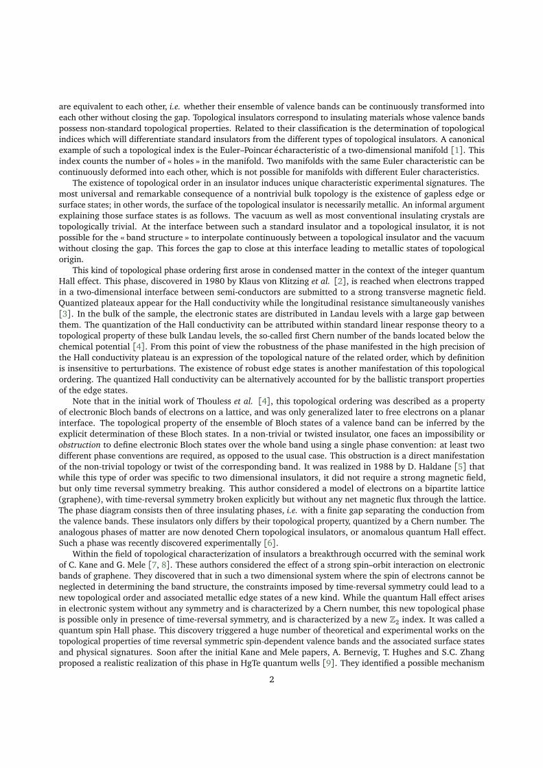
To provide an intuitive picture of nontrivial bundles, we will consider a simple example: the Möbius bundle[1]. Let us consider as the base manifold the circle S1, and let UN = (0− ε,π+ ε) and US = (−π− ε, 0+ ε) with
3
VEVW
UN
US
S1
Figure 1: Schematic view of the open covering (UN, US) of S1, with the intersections VE and VW of the open sets.
S1 S1
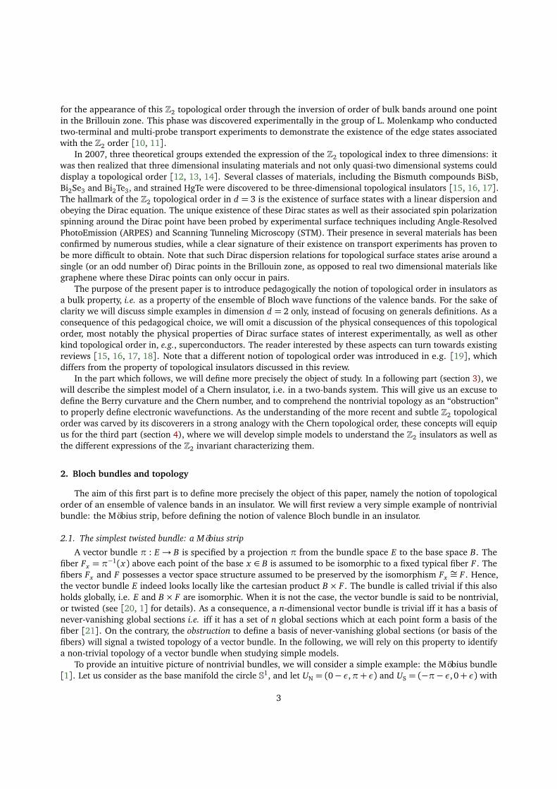
Figure 2: A cylinder (left) is a trivial bundle (with no twist), whereas a Möbius strip (right) is a nontrivial bundle (with twist). Here, we haveused the typical fiber F = [−1, 1] instead of R to get a compact manifold that is easier to draw.
ε > 0 be an open covering of S1 ' [0, 2π], parameterized by the angle θ ∈ S1 (see Fig. 1). Take the typical fiberto be the line F = R, parameterized by t ∈ F , and take as a structure group the two-elements group Z2 = {−1,1}.To construct a fibre bundle π : E→ S1 over S1, we have to glue together the products UN × F and US × F . Theintersection of the two open sets of the covering is UN ∩ US = VE ∪ VW with VE = (−ε,ε) and VW = (π− ε,π+ ε).The transition functions tN S(θ) can be either t 7→ t or t 7→ −t. If we choose both transition functions equal:
tN S(θ ∈ VE) : t 7→ t and tN S(θ ∈ VW) : t 7→ t (1)
the bundle π : E→ S1 is a trivial (nontwisted) bundle, which is a cylinder (Fig. 2, left). However, is we choosedifferent transition functions on each side:
tNS(θ ∈ VE) : t 7→ t and tNS(θ ∈ VW) : t 7→ −t (2)
the bundle is not trivial (it is twisted), and is the Möbius bundle (Fig. 2, right). This illustrates the relationbetween the triviality of the bundle and the choice of the transition function tNS. When the bundle can becontinuously deformed such that the transition functions be always the identity function the bundle will be trivial.
Let us illustrate on this example another property of a twisted bundle : the obstruction to define a basis ofnever-vanishing global sections in a twisted bundle. First, notice that as R is a one-dimensional vector space, theMöbius bundle is a one-dimensional (line) real vector bundle. Let s be a global section of the Möbius bundle.After one full turn from a generic position θ , we have crossed one transition function t 7→ t and one transitionfunction t 7→ −t so we have s(θ + 2π) =−s(θ ). Hence s = 0 everywhere : the only global section on the Möbiusbundle is the zero section. There is no global section of the Möbius bundle (except the zero section), so thisbundle is indeed nontrivial.
4
2.2. Bloch bundles
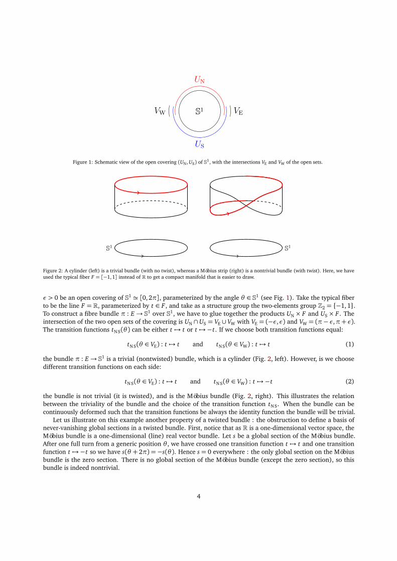
We consider a d-dimensional crystal in a tight-binding approach. We will describe its electronic propertiesusing a single electron Hamiltonian, i.e. neglecting interaction effects. Hence, from now on, we only focus onfirst-quantized one-particle Hamiltonians. The discrete real space lattice periodicity of this Hamiltonian reflectsitself into the nature of its eigenstates, which are Bloch wavefunctions indexed by a quasi-momentum k. Thisquasi-momentum k is restricted to the first Brillouin zone of the initial lattice: it is defined up to a reciprocal latticevector G. Hence this Brillouin zone has the topology of a d-dimensional torus Td , which we call the Brillouin torus.From the initial Hamiltonian, we deduce for each value of this quasi-momentum k a « Bloch Hamiltonian » H(k)acting on a 2n-dimensional Hilbert space, which accounts for the 2n electronic degrees of freedom in the unit cell(e.g. sites, orbitals, or spin). Associated with this Bloch Hamiltonian are its Bloch eigenstates and eigen-energiesEα(k), α= 1, . . . , 2n. The evolution of each Eα(k) as k evolves in the Brillouin torus defines a band. An insulatorcorresponds to the situation where a gap in energy separates the empty bands above the gap, from the filled bandsor valence bands below the gap (see Fig. 3). In this situation, when the chemical potential lies inside the gap,electronic states of the crystal cannot be excited by a small perturbation such as the application of the differenceof potential: no current can be created. The ground state of such an insulator is determined from the ensemble ofsingle particle eigenstates corresponding to the filled bands. These eigenstates are defined for each valence band,and for each point k of the Brillouin torus, up to a phase. The corresponding fiber bundle over the Brillouin zonedefined from the eigenstates of the valence bands is the object of study in the present paper.
0 π/2k
Eµ
insulator0 π/2k
E
µ
metal
Figure 3: Schematic band structures of an insulator (left) and a metal (right). The variable k corresponds to the coordinate on some genericcurve on the Brillouin torus.
Bloch Hamiltonians H(k) define for each k Hermitian operators on the effective Hilbert space Hk∼= C2n at k.
The collection of spaces Hk forms a vector bundle on the base space Td . This vector bundle happens to be alwaystrivial, hence isomorphic to Td ×C2n, at least for low dimensions of space d ≤ 3 (this is due to the vanishing ofthe total Berry curvature, see [22, 23]). This means that we may assume that the Bloch Hamiltonians H(k) arek-dependent Hermitian 2n× 2n matrices defined so that H(k) = H(k+ G) for G in the reciprocal lattice (notethat this does not always correspond to common conventions in particular on multi-partite lattices, see e.g. [24])
In an insulator, there are at least two well-defined subbundles of this complete trivial bundle: the valencebands bundle, which corresponds to all the filled bands, under the energy gap, and the conduction bands bundle,which corresponds to all the empty bands, over the energy gap. In the context of topological insulators, wewant to characterize the topology of the valence bands bundle, which underlies the ground state properties ofthe insulators. In a topological insulator this valence bands subbundle possesses a twisted topology while thecomplete bundle is trivial.
In the following, we will discuss two different kinds of topological orders. In the first one, we will discuss Cherninsulators (section 3): no symmetry constraints are imposed on the Bloch bundle, and in particular time-reversalinvariance is broken. In the second part, we will discuss Z2 insulators (section 4): here, time-reversal invariance is
5
preserved. In a time-reversal invariant system, the bundle of filled bands and the bundle of empty bands happento be separately trivial. However, the time-reversal invariance adds additional constraints on the bundle: evenif the filled bands bundle is always trivial as a vector bundle when time-reversal invariance is present, it is notalways trivial in a way which preserves a structure compatible with the time-reversal operator.
3. Chern topological insulators
3.1. IntroductionThe first example of a topological insulator is the quantum Hall effect (QHE) discovered in 1980 by von
Klitzing et al. [2]. Two years later, Thouless, Kohmoto, Nightingale, and de Nijs (TKNN) [4] showed that QHE ina two-dimensional electron gas in a strong magnetic field is related to a topological property of the filled band(see also [22, 25]). Namely, the Hall conductance is quantized, and proportional to a topological invariant of thefilled band named Chern number (hence the name Chern insulator). Haldane [5] has generalized this argumentto a system with time-reversal breaking without a net magnetic flux, hence without Landau levels. This kind ofChern insulator, which has recently been observed experimentally [6], is called quantum anomalous Hall effect.Chern insulators, with or without a net magnetic flux, only exist in two dimensions.
3.2. The simplest model: a two-bands insulatorThe simplest insulator possesses two bands, one above and one below the band gap. Such an insulator can
generically be described as a two-level system, which corresponds to a two-dimensional Hilbert space Hk ' C2 ateach point of the Brillouin torus, on which acts a Bloch Hamiltonian continuously defined on the Brillouin torus.Hence H(k) can be written as a 2× 2 Hermitian matrix, parameterized by the real functions hµ(z):
H(k) =�
h0 + hz hx − ihyhx + ihy h0 − hz
�
, (3)
which can re rewritten on the basis of Pauli matrices 1 plus the identity matrix σ0 = 1 as:
H(k) = hµ(k)σµ = h0(k)1+~h(k) · ~σ (4)
In the following, we always assumed that the coefficients hµ are well defined on Brillouin torus, i.e. are periodic.The spectral theorem ensures that H(k) has two orthogonal normalized eigenvectors u±(k) with eigenvalues ε±(k),which satisfy:
H(k)u±(k) = ε±(k)u±(k). (5)
Using Tr(H) = 2h0 and det(H) = h20 − h2 with h(k) = ‖~h(k)‖ =
Æ
h2x(k) + h2
y(k) + h2z(k) we obtain the energy
eigenvalues:
ε±(k) = h0(k)± h(k) (6)
The corresponding normalized eigenvectors are, up to a phase:
u±(k) =
1+hz + ε2
±
h2x + h2
y
!− 12
ε±
hx + ihy1
(7)
The energy shift of both energies has no effect on topological properties, provided the system remainsinsulating. To simplify the discussion, let us take h0 = 0. Therefore, the system is insulating provided h(k) nevervanishes on the whole Brillouin torus, which we enforce in the following. As we focus only on the topologicalbehavior of the filled band, which is now well-defined, we only consider the filled eigenvector u−(k) in thefollowing.
1. We use the usual convention that a greek index starts at 0 whereas a latin index starts at 1.
6
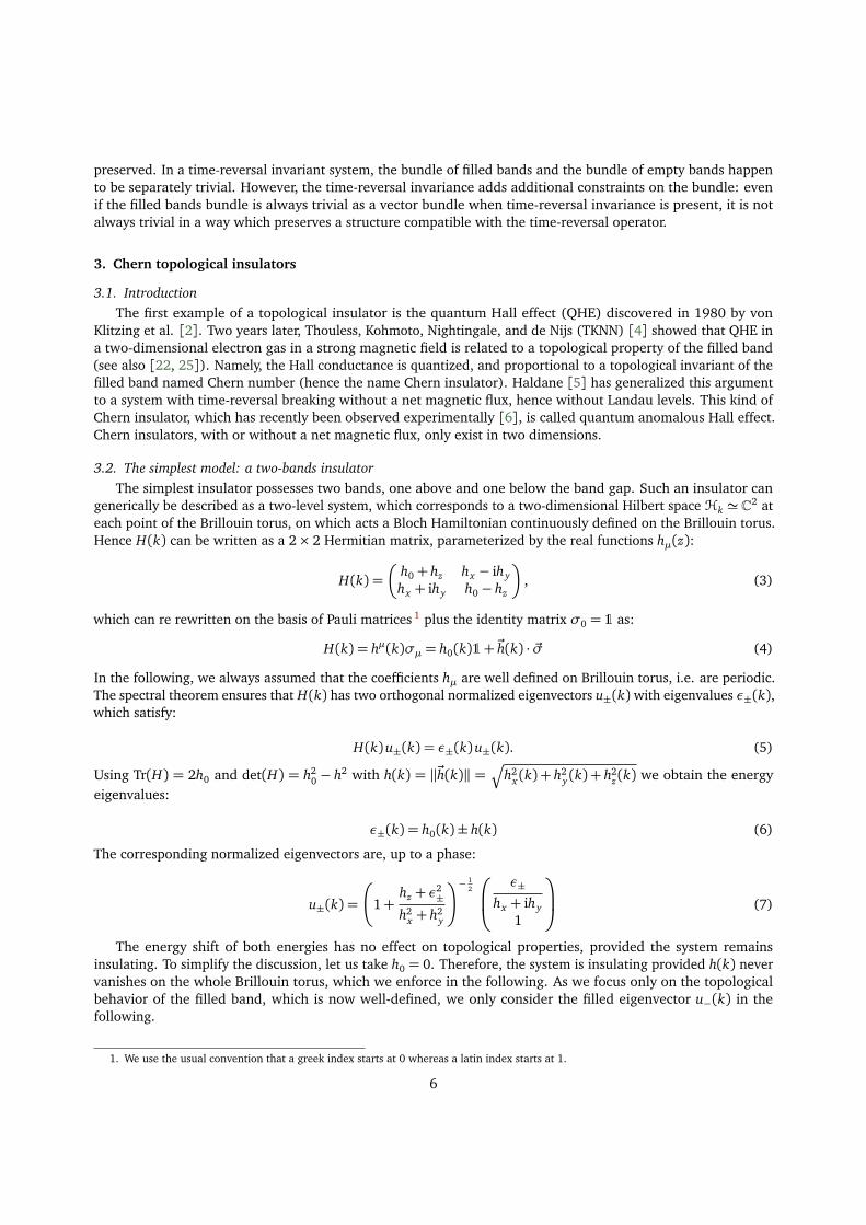
UN
US
C
Figure 4: Open covering (UN, US) of the sphere S2. The intersection C of the open sets is topologically a circle S1 and can be viewed as theboundary of either of the open sets.
3.3. An obstruction to continuously define the eigenstates
The filled band of the two-bands insulator is described by a map that assigns a filled eigenvector u−(k) to eachpoint of the Brillouin torus: it defines a one-dimensional complex vector bundle on the torus. When this vectorbundle is trivial, this map can be chosen to be continuous on the whole Brillouin torus: this corresponds to thestandard situation where a choice of phase for the Bloch eigenstate at a given point k0 of the Brillouin torus canbe continuously extrapolated to the whole torus. When it is not trivial, there is an obstruction to do so.
To clarify this notion of obstruction, let us first notice that the Hamiltonian (4) is parameterized by a three-dimensional real vector ~h. The energy shift h0 does not affect the topological properties of the system and hasbeen discarded. In spherical coordinates, this vector reads:
~h= h
sinθ cosϕsinθ sinϕ
cosθ
. (8)
With these coordinates, we rewrite the filled eigenvector (7) as:
u−(~h) =
�
− sin θ
2eiϕ cos θ
2
�
(9)
We notice that the norm h= ‖~h‖ of the parameter vector ~h does not affect the eigenvector. Therefore, theparameter space is a 2-sphere S2. We will first see in the following that there is always an obstruction to define acontinuous eigenvector u−(~h/h) on the sphere, or in other words, that the corresponding vector bundle on thesphere S2 is not trivial. Hence, we will realize that the original vector bundle on Brillouin torus (the pullbackbundle by ~h of the bundle on the sphere) is only nontrivial when the map k 7→~h(k) covers the whole sphere.
In the limit θ → 0, the eigenvector (9) is not well defined because it has an ill-defined phase. We could changeour phase convention and, e.g., multiply the eigenvector (9) by eiϕ, but this would only move the ill-defined limitto θ → π. It turns out that it is not possible to get rid of this singularity and define a continuous eigenvector onthe whole sphere. This behaviour unveils the nontrivial topology of a vector bundle on the sphere, discoveredby Dirac and Hopf in 1931 [26]: at least two local trivializations are needed to describe a vector bundle on thesphere [27, 1].
Let us choose an open covering (UN, US) of the sphere, the two open sets being the north hemisphere UN andthe south hemisphere US, chosen so that they have a nonzero intersection homotopy equivalent to the equatorcircle (Fig. 4). We define local trivializations of the filled band bundle by
uS−(~h) =
�
− sin θ
2eiϕ cos θ
2
�
and uN−(~h) =
�
−e−iϕ sin θ
2cos θ
2
�
(10)
7
Indeed, uN− is correctly defined on UN (resp. uS
− on US), but neither are well defined on the whole sphere.The intersection C = UN ∩ US can be reduced to a circle, and can be viewed as the boundary e.g. of UN, i.e.C = ∂ UN ' S1. The transition function from the trivialization on UN to the trivialization on US is phase change onthe equator, i.e. a map tNS : C→ U(1)
tNS = eiϕ (11)
Now let us recall that the Bloch electronic states are described by a bundle on the Brillouin torus. If themap ~h/h from the Brillouin torus to the parameter manifold does not completely cover the sphere (taking intoaccount the orientations, see below), there will be no obstruction to globally define eigenstates of the BlochHamiltonian, by smoothly deforming the pulled-back transition function h? tNS = tN S ◦ h to the identity. On thecontrary, if ~h/h does completely cover the sphere, the topology of the Bloch bundle is not trivial: it is neverpossible to deform the transition function to the identity. Those statements are indeed made quantitative throughthe introduction of the notion of Chern number.
3.4. Berry curvature and Chern numberAs the complete Bloch bundle (with filled and empty bands) is always trivial (see section 2.2), we can
indifferently study the topological properties of the filled band or of the empty one: the topology of the filled bandwill reflect the topological properties of the empty one. In the context of Bloch bundles, topological propertiesof the filled band are characterized by its Chern class (see [27, ch. 2] as well as [1, ch. 10] for a generalintroduction to the Berry phase, connection and curvature). The Chern classes are an intrinsic characterization ofthe considered bundle, and do not depend on a specific connection on it. However, in the context of condensedmatter and of Bloch systems, the Berry connection appears as a natural and particularly useful choice [28].
The Berry curvature A associated with the filled band k→ u−(k) is the 1-form defined by 2
A=1
i⟨u−|d u−⟩=−
1
i⟨d u−|u−⟩ (12)
where d is the exterior derivative. The Berry curvature is then
F = dA (13)
In the following, we consider only two-dimensional systems. In this case, the vector bundles are characterizedby the first Chern number c1, that can be computed as an integral of Berry curvature F over the Brillouin torus:
c1 =1
2π
∫
BZ
F. (14)
This integral of a 2-form is only defined on a 2-dimensional surface, and the Chern number characterisesinsulators in dimension d = 2 only. More generally, a quantum hall insulator only exists in even dimensions.
In order to relate the discussion of Chern insulators to the pictorial example of the Möbius strip (sec. 2.1,p. 3), we now express the first Chern number as the winding number of the transition function tN S introduced insec. 3.3. Indeed,
c1 =1
2π
∫
BZ
F =1
2π
∫
h−1(UN)
F +
∫
h−1(US)
F
=1
2π
∫
∂ h−1(UN)
h?AN +
∫
∂ h−1(US)
h?AS
=1
2π
∫
∂ h−1(UN)
�
h?AN − h?AS�
(15)
2. Note that Berry curvature is sometimes defined with an additional i factor, in which case it is purely imaginary.
8
where h?A= A◦ h represents the connection form defined on the sphere pulled back by the map h to be definedon the torus 3, and we used that ∂ h−1(UN) and ∂ h−1(US) have opposite orientations. We can now relate the Berryconnections on the two hemispheres with the transition function, by using (12) with the transition function (11),we get
AN = t−1NS AS tN S + t−1
NS
d
itNS = AS + dϕ (16)
so that
AN − AS = dϕ =1
id log(tN S). (17)
Finally, we obtain the expression of the Chern number as the winding of the transition function
c1 =1
2π
∫
BZ
F =1
2πi
∫
∂ h−1(UN)
d log(tNS ◦ h). (18)
Hence, the filled eigenvector as well as the associated Berry connection are well defined on the whole Brillouintorus only if the transition function tN S ◦ h : ∂ h−1(UN)→ U(1) can be continuously deformed to the identity, i.e.when it does not wind around the circle, which corresponds to a trivial Chern class c1 = 0. The first Chern numberis therefore the winding number of the transition function ; when the Chern class is not trivial, it is not possibleto deform the transition function to the identity. Notice that a nonzero first Chern number can be seen as anobstruction to Stokes theorem, as its expression (14) in terms of the Berry curvature would vanish if we couldwrite « F = dA » on the whole torus.
Let us now come back to our two-band model with the parameterization (4) where we have omitted the partproportional to the identity (h01) :
H(k) =~h(k) · ~σ (19)
In this case, the curvature 2-form takes the form [28]:
F =1
4εi jk h−3 hi dh j ∧ dhk, (20)
and the first Chern number reads:
c1 =1
2π
∫
BZ
F =1
2π
∫
BZ
1
4εi jk ‖h‖−3 hi dh j ∧ dhk. (21)
As ~h(~k) depends on the two components kx et ky of the wavevector, we have:
dh j =∂ h j
∂ kadka et dh j ∧ dhk =
∂ h j
∂ ka
∂ hk
∂ kbdka ∧ dkb (22)
The curvature F can be written in the more practical form:
F =1
4εi jk ‖h‖−3 hi
∂ h j
∂ ka
∂ hk
∂ kbdka ∧ dkb =
1
2
~h
‖h‖3 ·�
∂~h
∂ kx×∂~h
∂ ky
�
dkx ∧ dky , (23)
corresponding to the first Chern number
3. The attentive reader will notice that we actually considered a map h from the sphere to the sphere when assuming that h−1(UN) andh−1(US) defines a open covering of the manifold we consider. To be more precise, we should consider two maps : from the torus (BZ) to thesphere, and the map h from the sphere to the sphere. For the sake of simplicity, we have implicitly assumed in writing eq. (15) that the firstmap from the torus to the sphere was topologically trivial.
9
c1 =1
4π
∫
BZ
~h
‖h‖3 ·�
∂~h
∂ kx×∂~h
∂ ky
�
dkx ∧ dky (24)
One recognises in the expression (21) the index of the map ~h (see Appendix C). Hence, the first Chern numberc1 = deg(~h, 0). This identification provides a geometrical interpretation of the Chern number in the case oftwo-band insulators. When k spreads over Brillouin torus, ~h describes a closed surface Σ. The Chern number canthen be viewed as
– the (normalized) flux of a magnetic monopole located at the origin through the surface Σ– the number of times the surface Σ wraps around the origin (in particular, it is zero if the origin is « outside »Σ ; more precisely it is the homotopy class of Σ in the punctured space R3 − 0)
– the number of (algebraically counted) intersections of a ray coming from the origin with Σ, which is themethod used in [29].
3.5. Haldane’s model
3.5.1. General considerationsIn this section, we consider an explicit example of such a two band model displaying a topological insulating
phase, namely the model proposed by Haldane [5]. Besides its description using the semi-metallic graphene,Haldane’s model describes a whole class of simple two bands insulating phases with possibly a nontrivialtopological structure, and proposes a description of one of the simplest examples of a topological insulator,namely a Chern insulator. In this model, both inversion symmetry and time-reversal symmetry are simultaneouslybroken in a sheet of graphene. Inversion symmetry is broken by assigning different on-site energies to the twoinequivalent sublattices of the honeycomb lattice, while time-reversal invariance is lifted by local magnetic fluxesorganized so that the net flux per unit cell vanishes. Therefore, the first neighbors hopping amplitudes are notaffected by the magnetic fluxes, whereas the second neighbors hopping amplitudes acquire an Aharonov–Bohmphase.
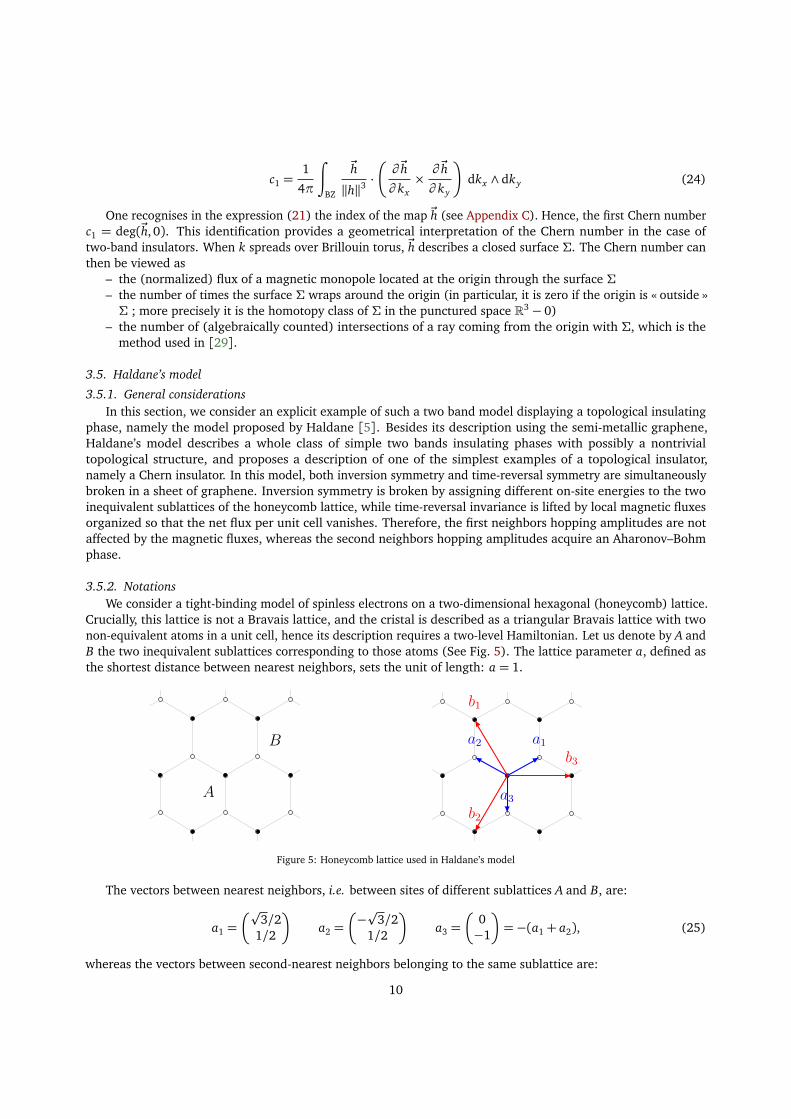
3.5.2. NotationsWe consider a tight-binding model of spinless electrons on a two-dimensional hexagonal (honeycomb) lattice.
Crucially, this lattice is not a Bravais lattice, and the cristal is described as a triangular Bravais lattice with twonon-equivalent atoms in a unit cell, hence its description requires a two-level Hamiltonian. Let us denote by A andB the two inequivalent sublattices corresponding to those atoms (See Fig. 5). The lattice parameter a, defined asthe shortest distance between nearest neighbors, sets the unit of length: a = 1.
A
B a1a2
a3
b1
b2
b3
Figure 5: Honeycomb lattice used in Haldane’s model
The vectors between nearest neighbors, i.e. between sites of different sublattices A and B, are:
a1 =�p
3/21/2
�
a2 =�
−p
3/21/2
�
a3 =�
0−1
�
=−(a1 + a2), (25)
whereas the vectors between second-nearest neighbors belonging to the same sublattice are:
10
b1 = a2 − a3 =�
−p
3/23/2
�
b2 = a3 − a1 =�
−p
3/2−3/2
�
b3 = a1 − a2 =�p
30
�
. (26)
Two of those vectors will serve as base vectors of the Bravais lattice ; we will choose b1 and b2. The reciprocallattice is then spanned by the two vectors b?1 and b?2 which satisfy:
bi b?j = 2πδi j , (27)
so
b?1 = 2π�
−1/p
31/3
�
b?2 = 2π�
−1/p
3−1/3
�
. (28)
Two points of the Brillouin zone are of particular interest in graphene, corresponding to the origin of thelow-energy Dirac dispersion relations. They are defined by:
K =1
2
�
b?1 + b?2�
and K ′ =−K . (29)
In the following, Gmn = mb?1 + nb?2 denotes an arbitrary reciprocal lattice vector (n, m ∈ Z).
3.5.3. Haldane’s HamiltonianThe first quantized Hamiltonian of Haldane’s model can be written as:
H = t∑
⟨ i, j ⟩
|i⟩ ⟨ j|+ t2
∑
⟪ i, j⟫|i⟩ ⟨ j|+M
∑
i∈A
|i⟩ ⟨i| −∑
j∈B
| j⟩ ⟨ j|
(30)
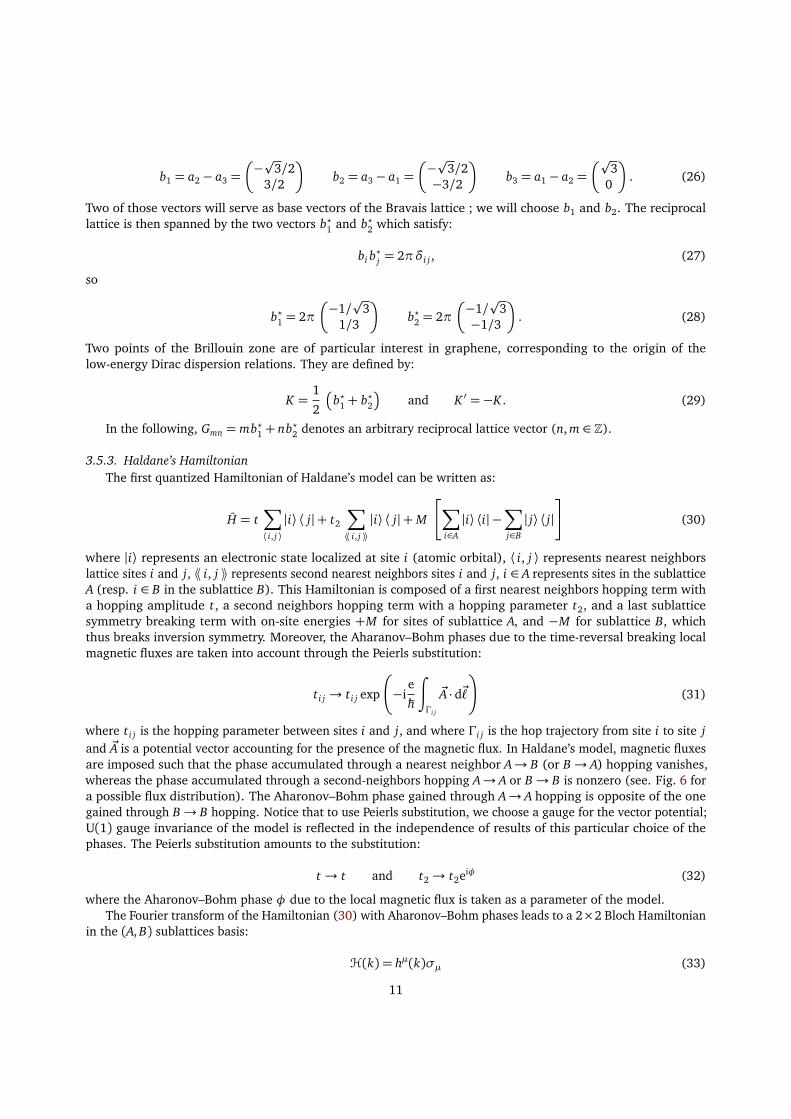
where |i⟩ represents an electronic state localized at site i (atomic orbital), ⟨ i, j ⟩ represents nearest neighborslattice sites i and j, ⟪ i, j ⟫ represents second nearest neighbors sites i and j, i ∈ A represents sites in the sublatticeA (resp. i ∈ B in the sublattice B). This Hamiltonian is composed of a first nearest neighbors hopping term witha hopping amplitude t, a second neighbors hopping term with a hopping parameter t2, and a last sublatticesymmetry breaking term with on-site energies +M for sites of sublattice A, and −M for sublattice B, whichthus breaks inversion symmetry. Moreover, the Aharanov–Bohm phases due to the time-reversal breaking localmagnetic fluxes are taken into account through the Peierls substitution:
t i j → t i j exp
−ie
ħh
∫
Γi j
~A · d~!
(31)
where t i j is the hopping parameter between sites i and j, and where Γi j is the hop trajectory from site i to site jand ~A is a potential vector accounting for the presence of the magnetic flux. In Haldane’s model, magnetic fluxesare imposed such that the phase accumulated through a nearest neighbor A→ B (or B→ A) hopping vanishes,whereas the phase accumulated through a second-neighbors hopping A→ A or B→ B is nonzero (see. Fig. 6 fora possible flux distribution). The Aharonov–Bohm phase gained through A→ A hopping is opposite of the onegained through B→ B hopping. Notice that to use Peierls substitution, we choose a gauge for the vector potential;U(1) gauge invariance of the model is reflected in the independence of results of this particular choice of thephases. The Peierls substitution amounts to the substitution:
t → t and t2→ t2eiφ (32)
where the Aharonov–Bohm phase φ due to the local magnetic flux is taken as a parameter of the model.The Fourier transform of the Hamiltonian (30) with Aharonov–Bohm phases leads to a 2×2 Bloch Hamiltonian
in the (A, B) sublattices basis:
H(k) = hµ(k)σµ (33)
11
−6ϕ ϕ
ϕ
ϕ
ϕ
ϕ
ϕ
Figure 6: Example of a choice for magnetic flux in an Haldane cell (left). We have used ϕ = φ/2 to simplify. Second-neighbors hoppingcorresponds to a nonzero flux (middle), whereas first-neighbors hopping gives a zero flux (right), so the total flux through a unit cell is zero.
with
h0 = 2t2 cosφ3∑
i=1
cos(k · bi) ; hz = M − 2t2 sinφ3∑
i=1
sin(k · bi) ; (34a)
hx = t�
1+ cos(k · b1) + cos(k · b2)�
; hy = t�
sin(k · b1)− sin(k · b2)�
; (34b)
with a convention where ~h is periodic: ~h(k+ Gmn) =~h(k).
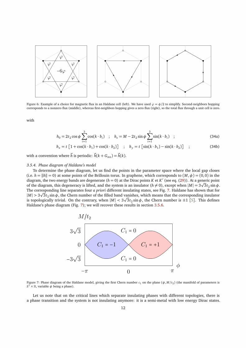
3.5.4. Phase diagram of Haldane’s modelTo determine the phase diagram, let us find the points in the parameter space where the local gap closes
(i.e. h= ‖h‖= 0) at some points of the Brillouin torus. In graphene, which corresponds to (M ,φ) = (0, 0) in thediagram, the two energy bands are degenerate (h= 0) at the Dirac points K et K ′ (see eq. (29)). At a generic pointof the diagram, this degeneracy is lifted, and the system is an insulator (h 6= 0), except when |M |= 3
p3t2 sinφ.
The corresponding line separates four a priori different insulating states, see Fig. 7. Haldane has shown that for|M |> 3
p3t2 sinφ, the Chern number of the filled band vanishes, which means that the corresponding insulator
is topologically trivial. On the contrary, when |M | < 3p
3t2 sinφ, the Chern number is ±1 [5]. This definesHaldane’s phase diagram (Fig. 7); we will recover these results in section 3.5.6.
−π 0 π
0
3√3
−3√3φ
M/t2
C1 = −1 C1 = +1C1 = 0
C1 = 0
Figure 7: Phase diagram of the Haldane model, giving the first Chern number c1 on the plane (φ, M/t2) (the manifold of parameters isS1 ×R, variable φ being a phase).
Let us note that on the critical lines which separate insulating phases with different topologies, there isa phase transition and the system is not insulating anymore: it is a semi-metal with low energy Dirac states.
12
M/t2
φC1 = −1 C1 = +1C1 = 0
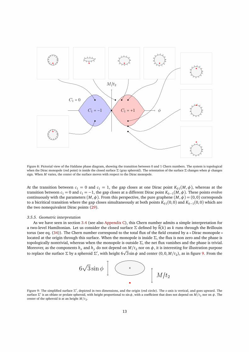
Figure 8: Pictorial view of the Haldane phase diagram, showing the transition between 0 and 1 Chern numbers. The system is topologicalwhen the Dirac monopole (red point) is inside the closed surface Σ (gray spheroid). The orientation of the surface Σ changes when φ changessign. When M varies, the center of the surface moves with respect to the Dirac monopole.
At the transition between c1 = 0 and c1 = 1, the gap closes at one Dirac point K01(M ,φ), whereas at thetransition between c1 = 0 and c1 =−1, the gap closes at a different Dirac point K0−1(M ,φ). These points evolvecontinuously with the parameters (M ,φ). From this perspective, the pure graphene (M ,φ) = (0, 0) correspondsto a bicritical transition where the gap closes simultaneously at both points K0 1(0,0) and K0−1(0,0) which arethe two nonequivalent Dirac points (29).
3.5.5. Geometric interpretationAs we have seen in section 3.4 (see also Appendix C), this Chern number admits a simple interpretation for
a two-level Hamiltonian. Let us consider the closed surface Σ defined by ~h(k) as k runs through the Brillouintorus (see eq. (34)). The Chern number correspond to the total flux of the field created by a « Dirac monopole »located at the origin through this surface. When the monopole is inside Σ, the flux is non zero and the phase istopologically nontrivial, whereas when the monopole is outside Σ, the net flux vanishes and the phase is trivial.Moreover, as the components hx and hy do not depend on M/t2 nor on φ, it is interesting for illustration purposeto replace the surface Σ by a spheroid Σ′, with height 6
p3sinφ and center (0, 0, M/t2), as in figure 9. From the
M/t26√3 sinφ
Figure 9: The simplified surface Σ′, depicted in two dimensions, and the origin (red circle). The z-axis is vertical, and goes upward. Thesurface Σ′ is an oblate or prolate spheroid, with height proportional to sinφ, with a coefficient that does not depend on M/t2 nor on φ. Thecenter of the spheroid is at an height M/t2.
13
evolution of this surface Σ′ as a function of M/t2 and φ, we identify easily Haldane’s phase diagram, see Fig. 7and Fig. 8. At a phase transition between two insulators with different Chern numbers, the origin necessarilycrosses the surface Σ, corresponding to a gap closing (i.e. h= ‖h‖ = 0) at least at one point on the Brillouin torus.Therefore, the topological phase transition is a semi-metallic phase.
3.5.6. Determination of the Chern numbers in the phase diagramTo determine in a more rigorous manner the topological phase diagram of Haldane model requires the
evaluation of the Chern number c11 as a function of the parameters (M/t2,φ). A simple method [29] consists inusing the geometric interpretation of the Chern number as the number of intersections between some ray comingfrom the origin and the oriented closed surface Σ spanned by h (see Appendix C). Alternatively, we can considerhalf of the number of intersections with a line instead of a ray. A natural choice for this line is the Oz axis. If D isthe set of pre-images by h of those intersections, i.e. D = h−1(Oz ∩Σ), the Chern number is:
c1 =1
2
∑
k∈D
sign [h(k) · n(k)] , (35)
where n(k) is the normal vector to Σ at k (where it is ±ez in the formula). We obtain (with a slight abuse ofnotation):
c1 =1
2
∑
k∈D
sign [F(k)] , (36)
where F is the Berry curvature from eq. (23). More explicitely, we obtain:
c1 =1
2
∑
k∈D
sign�
hz(k)�
sign
��
∂~h
∂ kx×∂~h
∂ ky
�
z
�
, (37)
the second term accounting for the direction of the normal. We now need to determine the set D, i.e. the set ofwavevectors k such that hx(k) = hy(k) = 0 (so that ~h lies the z axis). As the components hx and hy of (34) areM/t2 and φ independent, they are identical to those in pure graphene (which is the point (M/t2,φ) = (0,0)),these points are the Dirac points of graphene 4:
D =
¨
K =
�
− 4π3p
30
�
et K ′ =−K
«
. (38)
Hence the quantities we need to compute are the masses of the Dirac points:
hz(K) = M − 3p
3t2 sinφ and hz(K′) = M + 3
p3t2 sinφ, (39)
and the Chern number is thus given by:
c1 =1
2
�
sign�
M
t2+ 3p
3sin(φ)�
− sign�
M
t2− 3p
3sin(φ)��
, (40)
which corresponds to the original result of [5] (see also Fig. 7). Obviously this method is specific neither tographene nor to Haldane’s model; we can apply it very efficiently to two bands general models indexed by avector ~h, as it necessitate only to compute the sign of hz at points where hx and hy vanish.
4. As the Dirac points are on the boundary of the standard Brillouin zone, there appears six points on this Brillouin zone depicted in theplace, but only two inequivalent ones on the torus.
14
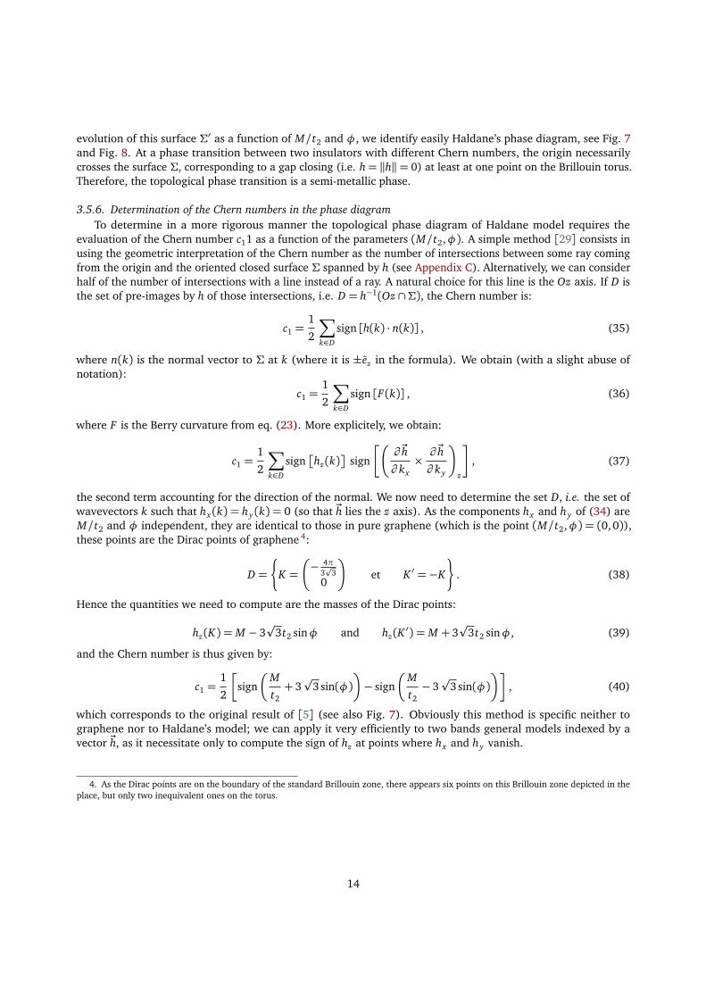
3.5.7. Surface statesOne of the crucial consequences of a nontrivial bulk topology is the appearance of metallic edge states at
the surface of a topological insulator. An sketchy way to understand the appearance of these surface states isthe following: as the Chern number is a topological quantity, it cannot change simply through a continuoustransformation, but only at a phase transition associated with a gap closing. Following [15] and [30], we discussthe appearance of edge states due to the change in bulk topology.
Let us start with a time-reversal invariant, parity-invariant system like graphene. The time-reversal symmetryimplies hz(k) = hz(−k), whereas the inversion symmetry implies hz(k) =−hz(−k). Hence when both symmetriesare present, hz identically vanishes. A Dirac point is an isolated point K of the Brillouin torus where the gapcloses i.e. h(K) = 0, so that the dispersion relation around this point is linear. Nielsen–Ninomiya’s theorem[31] implies that Dirac points come in pairs in a time-reversal invariant system. Hence, the simplest case is onewith two Dirac points K and K ′. This is the case of the Haldane model discussed in section 3.5. In Haldane’smodel, the time-reversal invariance is lifted. The gap at the Dirac points opens because hz(K) 6= 0, but we havestill hx(K) = hy(K) = 0. Hence, the Dirac points have gained a mass m = hz(K). Indeed, let us linearize theHamiltonian (4) around a Dirac point K by writing k = K + q :
Hl(q) = ħhvF q ·σ2d +mσz (41)
with q = (qx , qy) and σ2d = (σx ,σy), and m = hz(K). The linearization gives rise to a massive Dirac Hamiltonianwith mass m. In the following, we set ħhvF = 1. In Haldane’s model, we have (see eq.(34))
m= hz(K) = M − 3p
3t2 sinφ and m′ = hz(K′) = M + 3
p3t2 sinφ (42)
As c1 = (sign m− sign m′)/2, the masses m and m′ of the Dirac points K and K ′ have the same sign in the trivialcase, whereas they have opposite signs in the topological case.
Let us now consider an interface at y = 0 between a (nontrivial) Haldane insulator with a Chern numberc1 = 1 for y < 0 and a (trivial) insulator with c1 = 0 for y > 0. Necessarily, one of the masses changes sign at theinterface: m(y < 0)< 0 and m(y > 0)> 0, whereas the other one has a constant sign m′ > 0 (see Fig. 10). It isthen natural to set m(0) = 0, which implies that the gap closes at the interface. A more precise analysis shows thatthere are indeed surface states [15]. As the mass m depends on the position, it is more convenient to express thesingle-particle Hamiltonian in space representation. By inverting the Fourier transform in (41) (which amounts tothe replacement q→−i∇), we obtain the Hermitian Hamiltonian:
Hl =−i∇ ·σ2d +m(y)σz =�
m(y) −i∂x − ∂y−i∂x + ∂y −m(y)
�
. (43)
In order to get separable PDE, let us rotate the basis with the unitary matrix:
U =1p
2
�
1 11 −1
�
(44)
to obtain the Schrödinger equation:
U ·Hl · U−1�
αβ
�
=�
−i∂x ∂y +m(y)−∂y +m(y) i∂x
��
αβ
�
= E�
αβ
�
. (45)
This matrix equation corresponds to two separable PDE:
(−i∂x − E)α= S1 =−(∂y +m(y))β (46a)
(i∂x − E)β = S2 =−(−∂y +m(y))α (46b)
In order to obtain integrable solutions, the corresponding separations constants S1 and S2 must be zero. We canthen solve separately for α and β . For our choice of m(y), there is only one normalizable solution, which reads inthe original basis:
15
ψqx(x , y)∝ eiqx x exp
�
−∫ y
0
m(y ′)dy ′�
�
11
�
(47)
and has an energy E(qx) = EF + ħhvFqx . This solution is localized transverse to the interface where m changessign (see Fig. 10). The edge state crosses the Fermi energy at qx = 0, with a positive group velocity vF and thuscorresponds to a “chiral right moving” edge state. When considering a transition from an insulator with theopposite Chern number to the vacuum, one would get a “chiral left moving” edge state.
nontrivial insulator trivial insulator
y
m(y) and ∣ψ∣2
Figure 10: Schematic view of edge states at a Chern–trivial insulator interface. The mass m(y) (blue dashed line) and the wavefunction
amplitude�
�ψ�
�
2(red continuous line) are drawn along the coordinate y orthogonal to the interface y = 0.
3.6. Models with higher Chern numbers
O
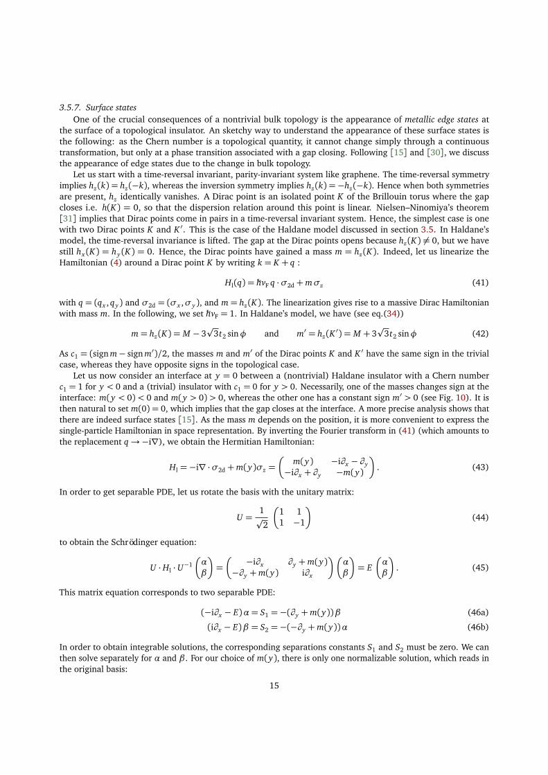
Figure 11: Let us consider a site at O. The nearest neighbors (from the opposite sublattice) are located on the dotted black circle. The secondneigbors (from the same sublattice) are on the blue dashed circle. The third neighbors are on the continuous red circle.
Topological phases with higher Chern numbers can be incorporated into Haldane’s model by consideringinteractions beyond second neighbors [29]. We briefly review an example with third nearest neighbors where theChern number can take values 0,±1,±2.
16
We consider a Haldane’s model with an additional interaction term between third nearest neighbors with ahopping amplitude t3 (see Fig. 11). The vector ~h(k) parametrizing the effective two-band model is then
h0 = 2t2 cosφ3∑
i=1
cos(k · bi); (48a)
hx = t�
1+ cos(k · b1) + cos(k · b2)�
+ t3�
2cos�
k ·�
b1 + b2��
+ cos�
k ·�
b1 − b2���
; (48b)
hy = t�
sin(k · b1)− sin(k · b2)�
+ t3 sin�
k ·�
b1 − b2��
; (48c)
hz = M − 2t2 sinφ3∑
i=1
sin(k · bi); (48d)
For a correctly choosen domain of t3, the Chern number can take the value�
�c1
�
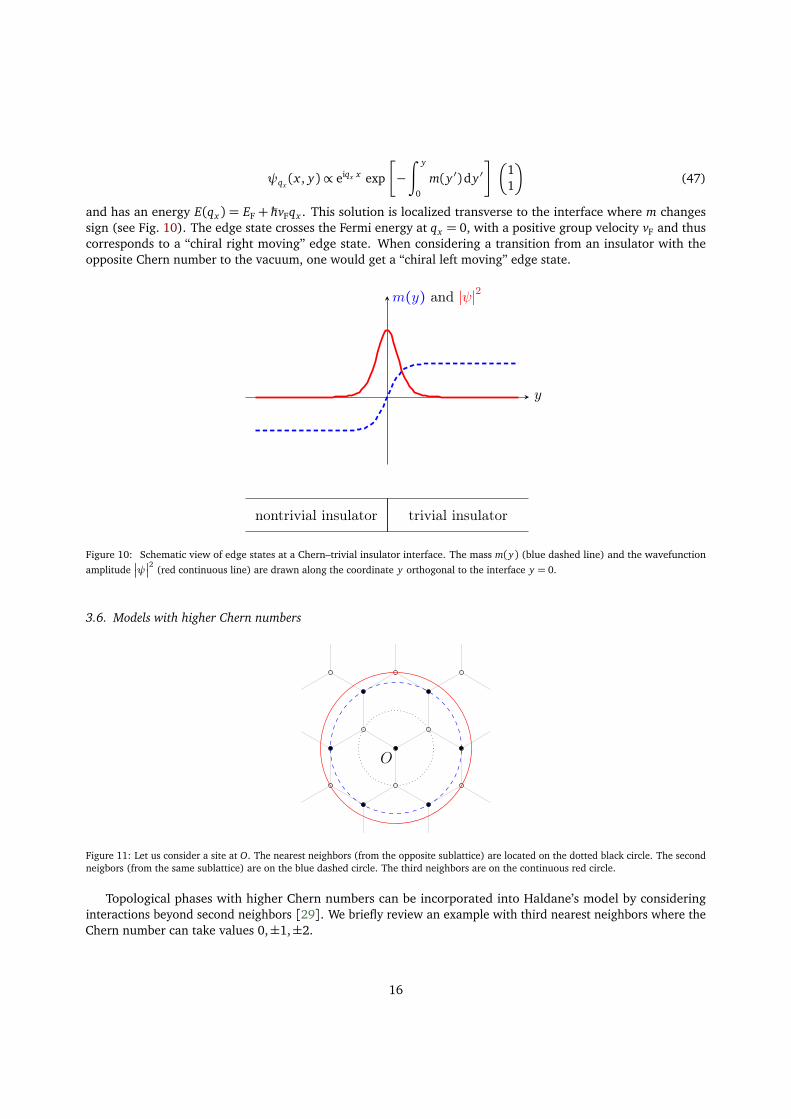
� = 2. The phase diagram in theplane (M/t2,φ) is drawn in Fig. 12. The geometric interpretation is essentially the same that in Haldane’s model,but the surface Σ can now wrap multiple times around the origin, corresponding to higher Chern numbers. Thesubtleties of the surface play an important role in the transitions: to hint at its evolution, we consider sections inthe planes xz and x y . The results are presented in Figs. 12 and 13.
−π 0 π
0
M/t2
φ
2 −2−1 1
−1 1
0
0
(a)
(b)
Figure 12: Schematic phase diagram of the extended Haldane model in the plane (M/t2,φ) for, e.g., t2/t1 = 0.5 and t3/t1 = 0.35 [29].Values of the Chern number are indicated as labels of the different phases. Arrows locate the topological transitions pictured in Fig. 13.
17
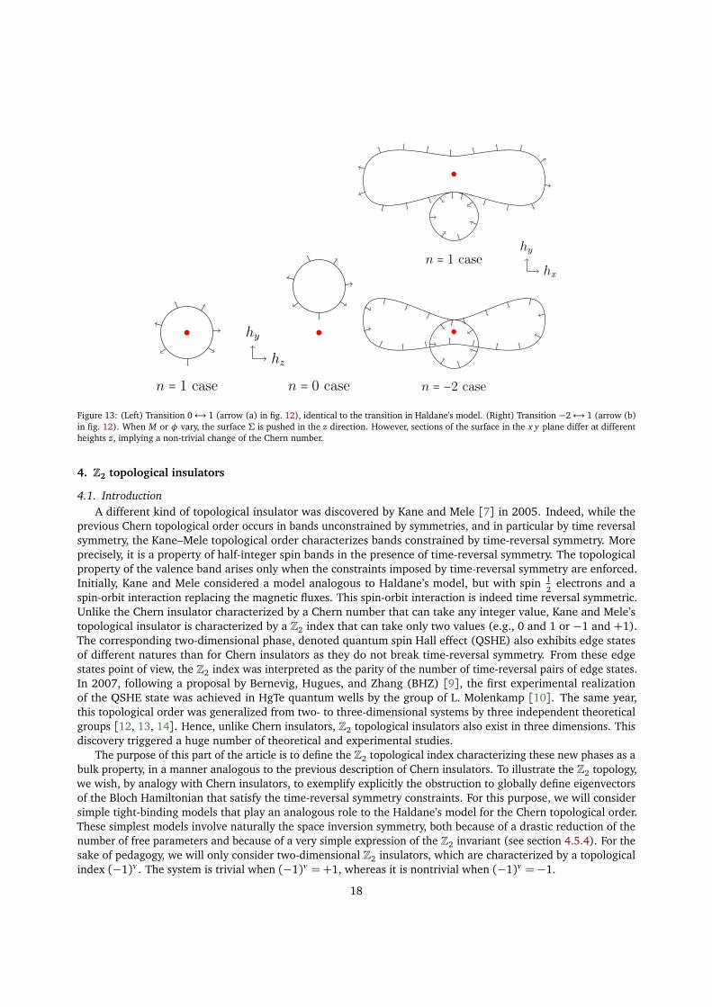
n = 1 case n = 0 case
hz
hy
n = 1 case
n = −2 case
hx
hy
Figure 13: (Left) Transition 0↔ 1 (arrow (a) in fig. 12), identical to the transition in Haldane’s model. (Right) Transition −2↔ 1 (arrow (b)in fig. 12). When M or φ vary, the surface Σ is pushed in the z direction. However, sections of the surface in the x y plane differ at differentheights z, implying a non-trivial change of the Chern number.
4. Z2 topological insulators
4.1. IntroductionA different kind of topological insulator was discovered by Kane and Mele [7] in 2005. Indeed, while the
previous Chern topological order occurs in bands unconstrained by symmetries, and in particular by time reversalsymmetry, the Kane–Mele topological order characterizes bands constrained by time-reversal symmetry. Moreprecisely, it is a property of half-integer spin bands in the presence of time-reversal symmetry. The topologicalproperty of the valence band arises only when the constraints imposed by time-reversal symmetry are enforced.Initially, Kane and Mele considered a model analogous to Haldane’s model, but with spin 1
2electrons and a
spin-orbit interaction replacing the magnetic fluxes. This spin-orbit interaction is indeed time reversal symmetric.Unlike the Chern insulator characterized by a Chern number that can take any integer value, Kane and Mele’stopological insulator is characterized by a Z2 index that can take only two values (e.g., 0 and 1 or −1 and +1).The corresponding two-dimensional phase, denoted quantum spin Hall effect (QSHE) also exhibits edge statesof different natures than for Chern insulators as they do not break time-reversal symmetry. From these edgestates point of view, the Z2 index was interpreted as the parity of the number of time-reversal pairs of edge states.In 2007, following a proposal by Bernevig, Hugues, and Zhang (BHZ) [9], the first experimental realizationof the QSHE state was achieved in HgTe quantum wells by the group of L. Molenkamp [10]. The same year,this topological order was generalized from two- to three-dimensional systems by three independent theoreticalgroups [12, 13, 14]. Hence, unlike Chern insulators, Z2 topological insulators also exist in three dimensions. Thisdiscovery triggered a huge number of theoretical and experimental studies.
The purpose of this part of the article is to define the Z2 topological index characterizing these new phases as abulk property, in a manner analogous to the previous description of Chern insulators. To illustrate the Z2 topology,we wish, by analogy with Chern insulators, to exemplify explicitly the obstruction to globally define eigenvectorsof the Bloch Hamiltonian that satisfy the time-reversal symmetry constraints. For this purpose, we will considersimple tight-binding models that play an analogous role to the Haldane’s model for the Chern topological order.These simplest models involve naturally the space inversion symmetry, both because of a drastic reduction of thenumber of free parameters and because of a very simple expression of the Z2 invariant (see section 4.5.4). For thesake of pedagogy, we will only consider two-dimensional Z2 insulators, which are characterized by a topologicalindex (−1)ν . The system is trivial when (−1)ν =+1, whereas it is nontrivial when (−1)ν =−1.
18
4.2. Time-reversal symmetry
4.2.1. The time-reversal operationTime-reversal operation amounts to the transformation in time t → −t. As such, quantities like spatial
position, energy, or electric field are even under time-reversal, whereas quantities like time, linear momentum,angular momentum, or magnetic field are odd under time-reversal operation. Within quantum mechanics, thetime-reversal operation is described by an anti-unitary operator Θ (which is allowed by Wigner’s theorem)[32, 33], that is to say (i) it is anti-linear, i.e. Θ(αx) = α?Θ(x) for α ∈ C and (ii) it satisfies Θ†Θ = 1, i.e.Θ† =Θ−1.
When spin degrees of freedom are included, time-reversal operation has to reverse the different spin expec-tation values: the corresponding standard representation of the time-reversal operator is [33] Θ = e−iπJy/ħh K,where Jy is the y component of the spin operator, and K is the complex conjugation (acting on the left). Fromthis expression, the time-reversal operator appears to be a π rotation in the spin space. Therefore, and becausethe spin operator e−iπJy/ħh is real and unaffected by K, in an integer spin system, the time-reversal operator isinvolutive, i.e. Θ2 = 1. However, for the 1
2-integer spin system, this operation is anti-involutive: Θ2 =−1. This
property will have crucial consequences in the following. As usual, a first quantized single-particle Hamiltonian H
is time-reversal invariant if it commutes with the time-reversal operator, i.e. [H,Θ] = 0.
4.2.2. Time-reversal symmetry in Bloch bandsIn the following, we consider the band theory of electrons in crystals [34], and hence we focus on the
case of spin 12
particles, with Θ2 = −1. Focusing on non-interacting electrons, we can describe the electronicbands through a first-quantized Hamiltonian, or equivalently through the Fourier-transformed effective BlochHamiltonian k→ H(k) defined on the Brillouin torus. In this context, the Bloch time-reversal operator Θ willrelate to the electronic Bloch states at k and −k, i.e. it is an anti-unitary map from the fiber at k to the fiber at −kof the vector bundle on the Brillouin torus that represents the bands of the system. In a time-reversal invariantsystem, the Bloch Hamiltonians at k and −k satisfy:
H(−k) = ΘH(k)Θ−1. (49)
As time-reversal operation maps a fiber at k to a fiber at −k, it is useful to consider the application on theBrillouin torus that relates the corresponding momenta: ϑ : T2→ T2, defined as ϑ k =−k on the torus, i.e. upto a lattice vector. The time-reversal operator is then viewed as a lift to this map ϑ on the total Bloch bundleT2 ×C2n describing the electronic states of all bands. It can be represented by an unitary matrix UΘ which doesnot depend on the momentum k on the Brillouin torus. Hence, it is a map:
T2 ×C2n→ T2 ×C2n
(k, v) 7→ (ϑk,Θv) = (−k, UΘK v)(50)
which sends the fiber of all bands Hk ' C2n at k to the fiber Hϑk at ϑk =−k. We sum that up by Θ : Hk →Hϑk.Notice that this implies that Θ2 =−1, indeed maps a fiber to itself.
In a time-reversal invariant system of spin 12
particles, the Berry curvature within valence bands is odd:Fα(k) =−Fα(−k). Hence the Chern number of the corresponding bands α vanishes: the valence vector bundle isalways trivial from the point of view of Chern indices. It is only when the constraints imposed by time-reversalsymmetry on the eigenstates are considered that a different kind of non-trivial topology can emerge.
4.2.3. Kramers pairsTime reversal implies the existence of Kramers pairs of eigenstates: equation (49) implies that the image by
time-reversal of any eigenstate of the Bloch Hamiltonian H(k) at k is an eigenstate of the Bloch HamiltonianH(−k) at −k, with the same energy. This is the Kramers theorem [33]. These two eigenstates, that a priori live indifferent fibers, are called Kramers partners. Θ2 =−1 implies that these two Kramers partners are orthogonal.Note that the orthogonality of these Kramers partners in different fibers has only a meaning if we embed thesefibers in the complete trivial bundle T2 ×C2n corresponding to the whole state space of the Bloch Hamiltonian.
19
E
k
µ
λ1 λ2 λ1
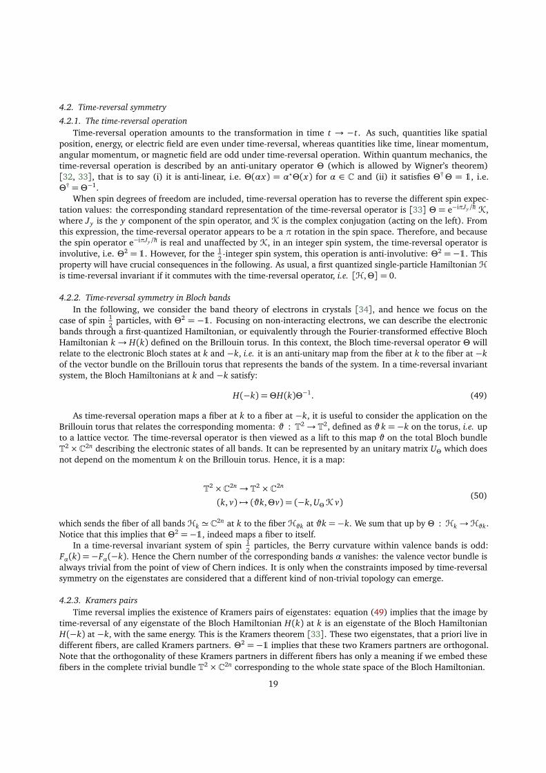
Figure 14: Typical energy spectrum of a time-reversal invariant system (continuous lines) on a closed loop of the Brillouin torus. At theTRIM λi , there is always a degeneracy of the filled bands (resp. empty bands). A Kramers pair is drawn as two black circles. When inversionsymmetry is present, the filled bands (resp. empty bands) are everywhere degenerate (dashed lines).
kx
ky
π
0
−ππ0−π
Figure 15: The four time-reversal invariant momenta in dimension d = 2: (0, 0), (π, 0), (0,π) et (π,π). The Brillouin torus T2 is representedas a primitive cell, whose sides must be glued together; points equivalent up to a lattice vector have been drawn with the same symbol.
20
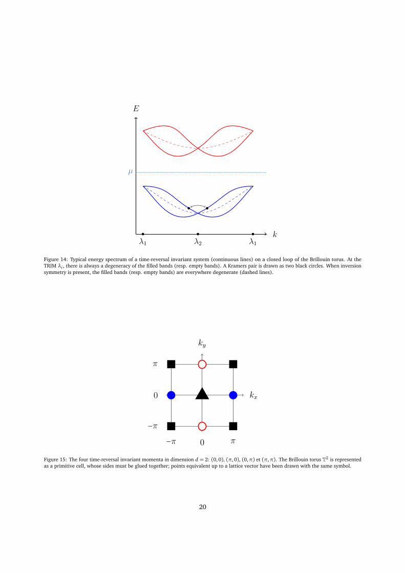
In view of the action of this time-reversal operation of the Bloch vector bundle, some points of the Brillouintorus appear of high interest: the points λ that are invariant under time-reversal [35], i.e. which verify λ =−λ+Gwhere G is a reciprocal lattice vector. Therefore, they are the points λ = G/2, with G a reciprocal lattice vector (seeFig. 15 for the example of a two dimensional square lattice). These points, usually named time-reversal invariantmomenta (TRIM), or high-symmetry points, are fixed points of ϑ and play an important role in time-reversalinvariant systems. In the following, we denote the set of TRIM as Λ. At these time reversal invariant points, thetwo partners of a Kramers pair live in the same fiber. As they are orthogonal and possess the same energy, thespectrum is necessarily always degenerate at these TRIM points (see Fig. 14). We will see in the following thatthe constraints imposed by the presence of these Kramers partners around the valence Bloch bundle are at theorigin of the Kane–Mele topological order.
4.2.4. Inversion symmetryIn the previous section, time-reversal symmetry was shown to relate fibers at k and −k around the Brillouin
torus. Hence, a particular spatial symmetry plays an important role when time reversal is at work: parity symmetry.The space inversion (or parity) P reverses the space coordinates, i.e. its action on coordinates is P~x =−~x . In aninversion symmetric crystal, the lattice is left globally invariant by the inversion operation P. However, differentsublattices are exchanged. Moreover P may act nontrivially on the Hilbert space of the internal degrees of freedomof the electronic states, depending on the atomic orbitals chosen to build the Bloch bands. Hence the explicitform of the parity operator will depend on the considered atomic basis. In the following, we will consider twoparticular cases of historical importance (with the bases (52)):
– the Kane–Mele model: a tight-binding model built out of identical atomic orbitals on a bipartite lattice. Inthis case, the parity operator is diagonal in the space of atomic orbitals: its only action is to exchange thesublattices, so P= σx ⊗1 (up to a global sign 5 that does not affect the topological properties);
– the Bernevig–Hughes–Zhang (BHZ) model: a tight-binding model built out of atomic orbitals with oppositeparity eigenvalues, but on a Bravais lattice. This corresponds to P = σz ⊗1 (e.g., the Bernevig–Hughes–Zhang model).
In the first case, σx exchanges the sublattices; in the second case, σz implements the parity eigenvalues of s and porbitals. In both cases, the spin remains obviously unaffected.
4.2.5. Simple four-band models and symmetriesWe are now in a position to define the simplest insulator with spin-dependent time-reversal bands. The
Kramers degeneracy imposes that they correspond to a pair of Kramers related bands below a gap, and pair ofKramers related bands above the gap (see Fig. 14). Hence the simplest model describing an insulator of electronswith spin and time-reversal symmetry is a four-level model. The Bloch Hamiltonian of a four-level system (e.g., atwo-level system with spin) is a 4× 4 Hermitian matrix. As a basis for the vector space of 4× 4 Hermitian matrix,we can choose to use the identity matrix 1, five Hermitian gamma matrices (Γa)1≤a≤5 which obey the Cliffordalgebra {Γa,Γb} = 2δa,b, and their commutators Γab = (2i)−1[Γa,Γb], ten of which are independent [35]. Insuch a basis, the Bloch Hamiltonian is parameterized by real function di(k), di j(k) as:
H(k) = d0(k)1 +5∑
i=1
di(k)Γi +∑
i> j
di j(k)Γi j (51)
The gamma matrices are constructed as tensor products of Pauli matrices that represent the two-level systemsassociated with a first degree of freedom and the spin of electrons. For the Kane–Mele model, the bipartite latticehas two sublattices A and B, corresponding to this first degree of freedom. In the BHZ model, this two-levelsystem consists of the two different orbitals s and p associated with each lattice site. The tensor product of asublattice (or orbital) basis (A, B) and a spin basis (↑,↓) provides the basis
(A, B)⊗ (↑,↓) = (A ↑, A ↓, B ↑, B ↓) or (s, p)⊗ (↑,↓) = (s ↑, s ↓, p ↑, p ↓) (52)
5. In the case of graphene, the parity eigenvalues of the pz orbitals is −1.
21
for the four-level system. The sublattice (orbital) operators are expanded on the basis (σi), and the spin ones areexpanded on (si), where σi and si are sublattice (orbital) and spin Pauli matrices, and the zeroth Pauli matrix istaken to be the identity matrix. With those choices, the time-reversal operator reads:
Θ= i (1⊗ sy)K. (53)
Several conventions are possible for the gamma matrices, and it is judicious to choose them so that thesymmetries of the Hamiltonian reflect into simple condition on the functions di(k), di j(k) [35]. The expression forthe Z2 invariant will turn out to be simpler for parity-invariant systems: this motivate our choice to impose thissymmetry. Following Fu and Kane [35], we choose the first gamma matrix Γ1 to correspond to the parity operator:Γ1 = P. Therefore, Γ1 is obviously even under P and also under Θ. This choice ensures that the other Γi matricesare odd under parity, i.e. PΓiP
−1 = ηi Γi with η1 = +1 and η j = −1 for j ≥ 2. Similarly, we obtain for the Γi j
matrices PΓi jP−1 = ηiη j Γi j . Let us now enforce the Γi≥2 matrices to be odd under time-reversal symmetry:
ΘΓiΘ−1 = ηi Γi . Due to the presence of i in their definition, the Γi j now follow a different rule under time-reversalsymmetry than under parity: ΘΓi jΘ−1 =−ηiη j Γi j Hence, with this convention, both P and Θ symmetries implyconsistent conditions on the function di(k): d1(k) is an even function around the TRIM points 6 : d1(k) = d1(−k),while the functions di (i > 1) are odd, i.e. di(k) =−di(−k). On the other hand, the parity conditions imposed onthe functions di j(k) by P and Θ symmetries are opposite to each other and cannot be simultaneously satisfied:the di j(k) must vanish. These constraints can equivalently be deduced from the behavior of the matrices underthe PΘ symmetry: with our choice, the Γi are even (PΘ) Γi (PΘ)−1 = Γi while their commutators are odd underPΘ: (PΘ) Γi j (PΘ)−1 =−Γi j .
Hence with the above conventions, we have reduced our study of PΘ invariant four band insulators from thegeneral Hamiltonian (51) to the simpler Hamiltonian:
H(k) = d0(k)1 +5∑
i=1
di(k)Γi . (54)
Note that because of the PΘ symmetry, the spectrum of such an Hamiltonian is everywhere degenerate (Fig. 14,dashed lines). In the general case, it reads:
E±(k) = d0(k)±
s
5∑
i=1
d2i (k) (55)
In the following, we neglect the d0 coefficient, which plays no role in the topological properties of the system.We will now turn to the detailed study of topological properties of two such four-band Hamiltonians. We
will use the notion of obstruction to illustrate the occurrence of topological order in the valence bands of thesemodels. Before proceeding, let us stress that in the presence of time-reversal symmetry, the bundle of filled bandsV is always trivial as a vector bundle. Hence, there is always a global basis of eigenstates |ui⟩1≤i≤2 of the valencebundle perfectly defined on the whole Brillouin torus. However, the valence bundle V is not always trivial whenendowed with the additional structure imposed by time reversal symmetry. Hence topological order will manifestitself as an impossibility to continuously define Kramers pairs on the whole Brillouin torus when the insulatoris nontrivial, that is to say, the global basis cannot satisfy Θ |u1(k)⟩ = |u2(−k)⟩. Hence, special care has to bedevoted to this Kramers constraints when determining the valence bands’ eigenstates. The aim of the followingsection is to demonstrate the occurrence of such an obstruction, before describing more general expressions of thetopological index.
6. On the Brillouin torus, the odd or even behaviour of a function happens around any TRIM. Let us consider a function f and supposethat we have f (k) = f (−k) for all k. Let λ ∈ Λ be a time-reversal invariant point. We have then λ =−λ, so f (λ+ k) = f (−λ− k) = f (λ− k)for any k. Hence, if f is even, it is also “even” around any TRIM. It obviously also works for an odd function.
22
kx
ky
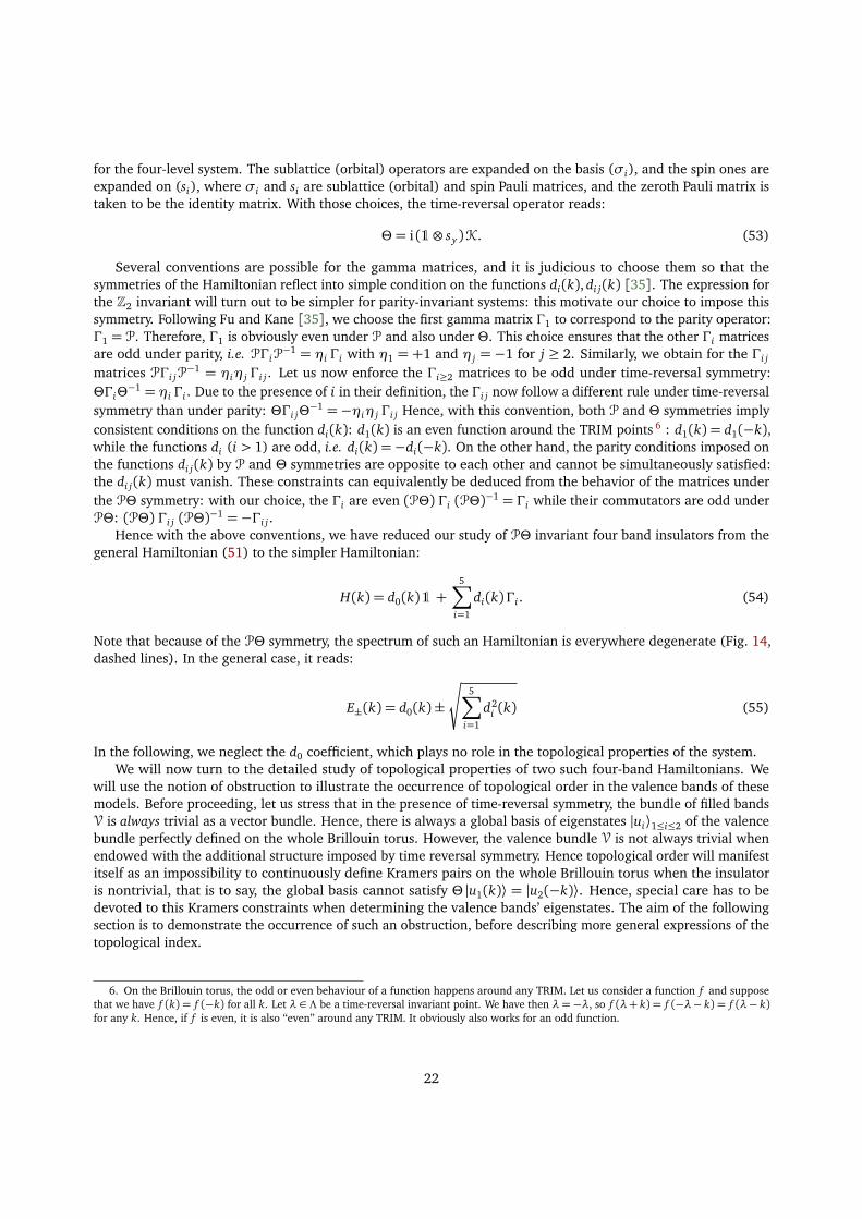
Figure 16: Examples of lines of zero of d1 (continuous blue) and d2 (dashed red) in the topological case, where d1 is only negative (or onlypositive) at the origin. For simplicity, these lines have been represented as straight lines, without loss of generality. At the intersections (greenpoints) where d1 = d2 = 0, singularities of the globally defined Kramers pairs of eigenvectors appear. These singularities cannot be removedby continuously deforming the parameters, unless the gap closes or the time-reversal invariance is broken.
4.3. Atomic orbitals of identical parity: Kane–Mele-like model
4.3.1. Minimal modelLet us consider a time-reversal invariant band insulator on an inversion symmetric bipartite lattice with
spin, such as the Kane–Mele model introduced in [7] and [35]. We work in the « sublattice tensor spin » basis(A ↑, A ↓, B ↑, B ↓), where the parity operator only exchanges A and B sites:
P= σx ⊗1 (56)
The model is written in the form of eq. (54), with the gamma matrices chosen to be:
Γ1 = P= σx ⊗1 Γ2 = σy ⊗1 Γ3 = σz ⊗ sx Γ4 = σz ⊗ sy Γ5 = σz ⊗ sz (57)
Following the discussion in the precious section 4.2.5, the parity and time-reversal constraints imply d1(k) to bean even function in the Brillouin torus, while the di≥2(k) are odd functions. Hence, all di except d1 vanish at thetime reversal invariants points. Moreover, the functions di≥2(k) should vanish around time-reversal invariant linesconnecting those TRIM (see Fig. 16).
For the system to remain insulating, and due to the vanishing of the di≥2(λ), we must have d1(λ) 6= 0 for allTRIM λ ∈ Λ. The quantities d1(λ) correspond to the opposite of the parity eigenvalues ξ(λ) of the bands at theTRIM 7. In the following, we will try to convince the reader that the bulk invariant unveiled by Fu and Kane (seesection 4.5.4):
∏
λ∈Λ
sign d1(λ) (58)
is indeed a topological index related to the obstruction to globally define Kramers pairs (especially of eigenvectorsof the Bloch Hamiltonian). Hence, for the model to display a topological insulating phase, the function d1(k)cannot take values of same sign at all the TRIM. Hence, this function should vanish somewhere on the Brillouintorus. As d1 is even, it will typically vanish on a time-reversal invariant loop around one or several TRIM. Hence,to keep the gap open, at least two non-zero coefficients di≥2 are needed (see Fig. 16). As these functions di≥2 areodd, they vanish on time-reversal invariant curves connecting the TRIM which cross necessarily the loop where d1
7. The energy of filled bands is always negative (with d0 = 0). Thus, at a TRIM λ, the parity eigenvalue of the filled states is the oppositeof the sign of the coefficient d1(λ). This is because E(λ) |u⟩= d1(λ)Γ1 |u⟩= d1(λ)ξ(λ) |u⟩ so E(λ) = d1(λ)ξ(λ). As the state is filled, wehave E(λ)< 0, so we get sign[ξ(λ)] =− sign[d1(λ)].
23
vanishes. With only one nonzero function da in addition to d1, there are always crossing points where the gapvanishes, at the intersections of the d1 = 0 loops and the di≥2 = 0 curves. Thus, to impose an insulating state, weneed to consider a minimal model with at least two functions di≥2. To sum up, the simplest description of aninsulating state with a possibly nontrivial topology is parameterized through eq. (54) by three nonzero functions:d1 and two additional functions di≥2. The simplest such example consists of choosing nonzero d1, d2, and d5values, as this choice preserves the spin quantum numbers. It is precisely the case considered by Fu and Kane[35] to describe an inversion symmetric version of the Kane and Mele’s model of graphene.
4.3.2. ObstructionThe filled normalized eigenstates with energy −‖d‖ =−
p
d21 + d2
2 + d25 for the model defined in the previous
section are, up to a phase 8:
|u1⟩=1
N1
0−d5 −‖d‖
0d1 + id2
and |u2⟩=1
N2
d5 −‖d‖0
d1 + id20
, (59)
where N j(~d) are positive coefficients ensuring that the vectors are normalized. Those vectors are obviouslyorthogonal, and thus form an orthonormal basis of the space of filled bands. We can easily verify that they alsoform Kramers pairs, i.e. that Θ |u1(k)⟩= |u2(−k)⟩. To do so, let us note that if |u j[~d]⟩ is an eigenvector at k, thecorresponding eigenvector at −k is obtained by changing the sign of all components of ~d except d1. Note that anaive point-wise diagonalisation of the Hamiltonian does not automatically provide Kramers pairs in the inversionsymmetric case, in particular when d3, d4 are nonzero, i.e. when the spin projection sz is not conserved. Theeasiest and systematic procedure is then to remove the additional degeneracy by introducing an infinitesimalparity-breaking, time-reversal invariant perturbation, such as a constant d12.
From (59), we infer that the limit of these eigenstates is ill-defined when d1, d2→ 0. To analyze this limit, weconsider the polar decomposition d1 + id2 = t eiθ , to obtain:
|u1⟩=1
N1
0
−d5 −�
�d5
�
�
p
1+ (t/d5)2
0teiθ
and |u2⟩=1
N2
d5 −�
�d5
�
�
p
1+ (t/d5)2
0teiθ
0
. (60)
In the limit t → 0 (while keeping the vectors normalized), we obtain (see Appendix E for details):
|u1⟩ →
0−100
and |u2⟩ →
00
eiθ
0
for d5 > 0, (61a)
and
|u1⟩ →
000
eiθ
and |u2⟩ →
−1000
for d5 < 0. (61b)
The phase θ is ill-defined when t → 0, so one of these eigenstates is ill-defined at the points where d1 = d2 = 0 areill-defined. It is possible to show that such a singularity cannot be removed by a U(2) change of basis preservingthe Kramers pairs structure (see also [36] for a related point of view).
8. Notice that this expression only stands when d4 = d3 = 0.
24
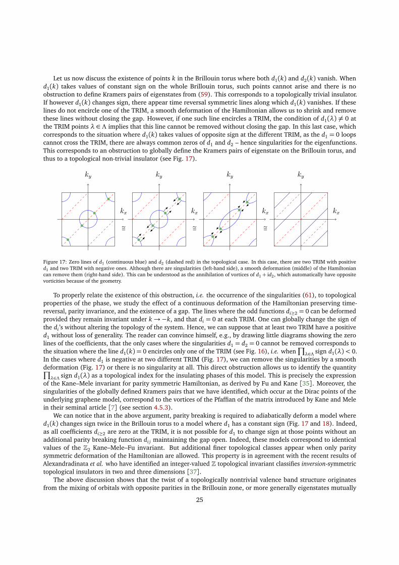
Let us now discuss the existence of points k in the Brillouin torus where both d1(k) and d2(k) vanish. Whend1(k) takes values of constant sign on the whole Brillouin torus, such points cannot arise and there is noobstruction to define Kramers pairs of eigenstates from (59). This corresponds to a topologically trivial insulator.If however d1(k) changes sign, there appear time reversal symmetric lines along which d1(k) vanishes. If theselines do not encircle one of the TRIM, a smooth deformation of the Hamiltonian allows us to shrink and removethese lines without closing the gap. However, if one such line encircles a TRIM, the condition of d1(λ) 6= 0 atthe TRIM points λ ∈ Λ implies that this line cannot be removed without closing the gap. In this last case, whichcorresponds to the situation where d1(k) takes values of opposite sign at the different TRIM, as the d1 = 0 loopscannot cross the TRIM, there are always common zeros of d1 and d2 – hence singularities for the eigenfunctions.This corresponds to an obstruction to globally define the Kramers pairs of eigenstate on the Brillouin torus, andthus to a topological non-trivial insulator (see Fig. 17).
kx
ky
≅kx
ky
≅kx
ky
≅kx
ky
Figure 17: Zero lines of d1 (continuous blue) and d2 (dashed red) in the topological case. In this case, there are two TRIM with positived1 and two TRIM with negative ones. Although there are singularities (left-hand side), a smooth deformation (middle) of the Hamiltoniancan remove them (right-hand side). This can be understood as the annihilation of vortices of d1 + id2, which automatically have oppositevorticities because of the geometry.
To properly relate the existence of this obstruction, i.e. the occurrence of the singularities (61), to topologicalproperties of the phase, we study the effect of a continuous deformation of the Hamiltonian preserving time-reversal, parity invariance, and the existence of a gap. The lines where the odd functions di≥2 = 0 can be deformedprovided they remain invariant under k→−k, and that di = 0 at each TRIM. One can globally change the sign ofthe di ’s without altering the topology of the system. Hence, we can suppose that at least two TRIM have a positived1 without loss of generality. The reader can convince himself, e.g., by drawing little diagrams showing the zerolines of the coefficients, that the only cases where the singularities d1 = d2 = 0 cannot be removed corresponds tothe situation where the line d1(k) = 0 encircles only one of the TRIM (see Fig. 16), i.e. when
∏
λ∈Λ sign d1(λ)< 0.In the cases where d1 is negative at two different TRIM (Fig. 17), we can remove the singularities by a smoothdeformation (Fig. 17) or there is no singularity at all. This direct obstruction allows us to identify the quantity∏
λ∈Λ sign d1(λ) as a topological index for the insulating phases of this model. This is precisely the expressionof the Kane–Mele invariant for parity symmetric Hamiltonian, as derived by Fu and Kane [35]. Moreover, thesingularities of the globally defined Kramers pairs that we have identified, which occur at the Dirac points of theunderlying graphene model, correspond to the vortices of the Pfaffian of the matrix introduced by Kane and Melein their seminal article [7] (see section 4.5.3).
We can notice that in the above argument, parity breaking is required to adiabatically deform a model whered1(k) changes sign twice in the Brillouin torus to a model where d1 has a constant sign (Fig. 17 and 18). Indeed,as all coefficients di≥2 are zero at the TRIM, it is not possible for d1 to change sign at those points without anadditional parity breaking function di j maintaining the gap open. Indeed, these models correspond to identicalvalues of the Z2 Kane–Mele–Fu invariant. But additional finer topological classes appear when only paritysymmetric deformation of the Hamiltonian are allowed. This property is in agreement with the recent results ofAlexandradinata et al. who have identified an integer-valued Z topological invariant classifies inversion-symmetrictopological insulators in two and three dimensions [37].
The above discussion shows that the twist of a topologically nontrivial valence band structure originatesfrom the mixing of orbitals with opposite parities in the Brillouin zone, or more generally eigenstates mutually
25
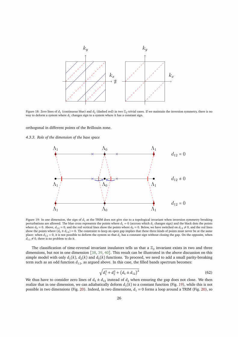
kx
ky
≇ kx
ky
Figure 18: Zero lines of d1 (continuous blue) and d2 (dashed red) in two Z2-trivial cases. If we maintain the inversion symmetry, there is noway to deform a system where d1 changes sign to a system where it has a constant sign.
orthogonal in different points of the Brillouin zone.
4.3.3. Role of the dimension of the base space
Λ0Λ1 Λ1
d12 = 0
Λ0Λ1 Λ1
d12 ≠ 0
Λ0Λ1 Λ1
d12 = 0
Figure 19: In one dimension, the sign of d1 at the TRIM does not give rise to a topological invariant when inversion symmetry breakingperturbations are allowed. The blue cross represents the points where d1 = 0 (accross which d1 changes sign) and the black dots the pointswhere d2 = 0. Above, d1 2 = 0, and the red vertical lines show the points where d5 = 0. Below, we have switched on d1 2 6= 0, and the red linesshow the points where (d5 ± d1 2) = 0. The constraint to keep an open gap implies that these three kinds of points must never be at the sameplace: when d12 = 0, it is not possible to deform the system so that d1 has a constant sign without closing the gap. On the opposite, whend12 6= 0, there is no problem to do it.
The classification of time-reversal invariant insulators tells us that a Z2 invariant exists in two and threedimensions, but not in one dimension [38, 39, 40]. This result can be illustrated in the above discussion on thissimple model with only d1(k), d2(k) and d5(k) functions. To proceed, we need to add a small parity-breakingterm such as an odd function d12, as argued above. In this case, the filled bands spectrum becomes:
Æ
d21 + d2
2 +�
d5 ± d12�2 (62)
We thus have to consider zero lines of d5 ± d12 instead of d2 when ensuring the gap does not close. We thenrealize that in one dimension, we can adiabatically deform d1(k) to a constant function (Fig. 19), while this is notpossible in two dimensions (Fig. 20). Indeed, in two dimensions, d1 = 0 forms a loop around a TRIM (Fig. 20), so
26
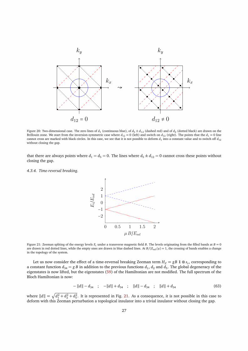
kx
ky
d12 = 0
↝ kx
ky
d12 ≠ 0
Figure 20: Two-dimensional case. The zero lines of d1 (continuous blue), of d5 ± d1 2 (dashed red) and of d2 (dotted black) are drawn on theBrillouin zone. We start from the inversion-symmetric case where d12 = 0 (left) and switch on d12 (right). The points that the d1 = 0 linecannot cross are marked with black circles. In this case, we see that it is not possible to deform d1 into a constant value and to switch off d12without closing the gap.
that there are always points where d1 = d5 = 0. The lines where d5 ± d12 = 0 cannot cross these points withoutclosing the gap.
4.3.4. Time-reversal breaking.
0 0.5 1 1.5 2
−2−10
1
2
µB/Eref
Ei/E r
ef
Figure 21: Zeeman spliting of the energy levels Ei under a transverse magnetic field B. The levels originating from the filled bands at B = 0are drawn in red dotted lines, while the empty ones are drawn in blue dashed lines. At B/(Eref/µ) = 1, the crossing of bands enables a changein the topology of the system.
Let us now consider the effect of a time-reversal breaking Zeeman term HZ = gB 1⊗ sz , corresponding toa constant function d34 = g B in addition to the previous functions d1, d2 and d5. The global degeneracy of theeigenstates is now lifted, but the eigenstates (59) of the Hamiltonian are not modified. The full spectrum of theBloch Hamiltonian is now:
−‖d‖− d34 ; −‖d‖+ d34 ; ‖d‖− d34 ; ‖d‖+ d34 (63)
where ‖d‖ =p
d21 + d2
2 + d25 . It is represented in Fig. 21. As a consequence, it is not possible in this case to
deform with this Zeeman perturbation a topological insulator into a trivial insulator without closing the gap.
27
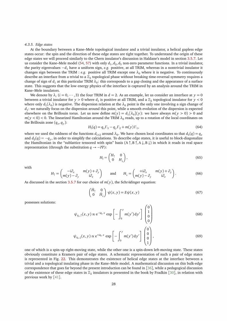
4.3.5. Edge statesAt the boundary between a Kane–Mele topological insulator and a trivial insulator, a helical gapless edge
states occur: the spin and the direction of these edge states are tight together. To understand the origin of theseedge states we will proceed similarly to the Chern insulator’s discussion in Haldane’s model in section 3.5.7. Letus consider the Kane–Mele model (54, 57) with only d1, d2, d5 non-zero parameter functions. In a trivial insulator,the parity eigenvalues −d1 have a uniform sign, e.g. positive, at all TRIM, whereas in a nontrivial insulator itchanges sign between the TRIM : e.g. positive all TRIM except one λ0 where it is negative. To continuouslydescribe an interface from a trivial to a Z2 topological phase without breaking time-reversal symmetry requires achange of sign of d1 at this particular TRIM λ0: this corresponds to a gap closing and the appearance of a surfacestate. This suggests that the low energy physics of the interface is captured by an analysis around the TRIM inKane–Mele insulators.
We denote by λi (i = 0, · · · , 3) the four TRIM in d = 2. As an example, let us consider an interface at y = 0between a trivial insulator for y > 0 where d1 is positive at all TRIM, and a Z2 topological insulator for y < 0where only d1(λ0) is negative. The dispersion relation at the λ0 point is the only one involving a sign change ofd1: we naturally focus on the dispersion around this point, while a smooth evolution of the dispersion is expectedelsewhere on the Brillouin torus. Let us now define m(y) = d1[λ0](y): we have always m(y > 0) > 0 andm(y < 0)< 0. The linearized Hamiltonian around the TRIM λ0 reads, up to a rotation of the local coordinates onthe Brillouin zone (qx , qy):
Hl(q) = qxΓ5 − qyΓ2 +m(y)Γ1, (64)
where we used the oddness of the functions di≥2 around λ0. We have chosen local coordinates so that d5(q) = qxand d2(q) =−qy , in order to simplify the calculations. To describe edge states, it is useful to block-diagonalizethe Hamiltonian in the “sublattice tensored with spin” basis (A ↑, B ↑, A ↓, B ↓) in which it reads in real spacerepresentation (through the substitution q→−i∇):
Hl =�
H↑ 00 H↓
�
, (65)
with
H↑ =�
−i∂x m(y) + ∂ym(y)− ∂y i∂x
�
and H↓ =�
+i∂x m(y) + ∂ym(y)− ∂y i∂x
�
. (66)
As discussed in the section 3.5.7 for our choice of m(y), the Schrödinger equation:�
H↑ 00 H↓
�
ψ(x , y) = Eψ(x , y) (67)
possesses solutions:
ψqx ,↑(x , y)∝ e−iqx x exp
�
−∫ y
0
m(y ′)dy ′�
0100
(68)
ψqx ,↓(x , y)∝ e+iqx x exp
�
−∫ y
0
m(y ′)dy ′�
0001
, (69)
one of which is a spin-up right-moving state, while the other one is a spin-down left-moving state. These statesobviously constitute a Kramers pair of edge states. A schematic representation of such a pair of edge statesis represented in Fig. 22. This demonstrates the existence of helical edge states at the interface between atrivial and a topological insulating phase in the Kane–Mele model. A mathematical discussion on this bulk-edgecorrespondence that goes far beyond the present introduction can be found in [36], while a pedagogical discussionof the existence of these edge states in Z2 insulators is presented in the book by Fradkin [30], in relation withprevious work by [41].
28
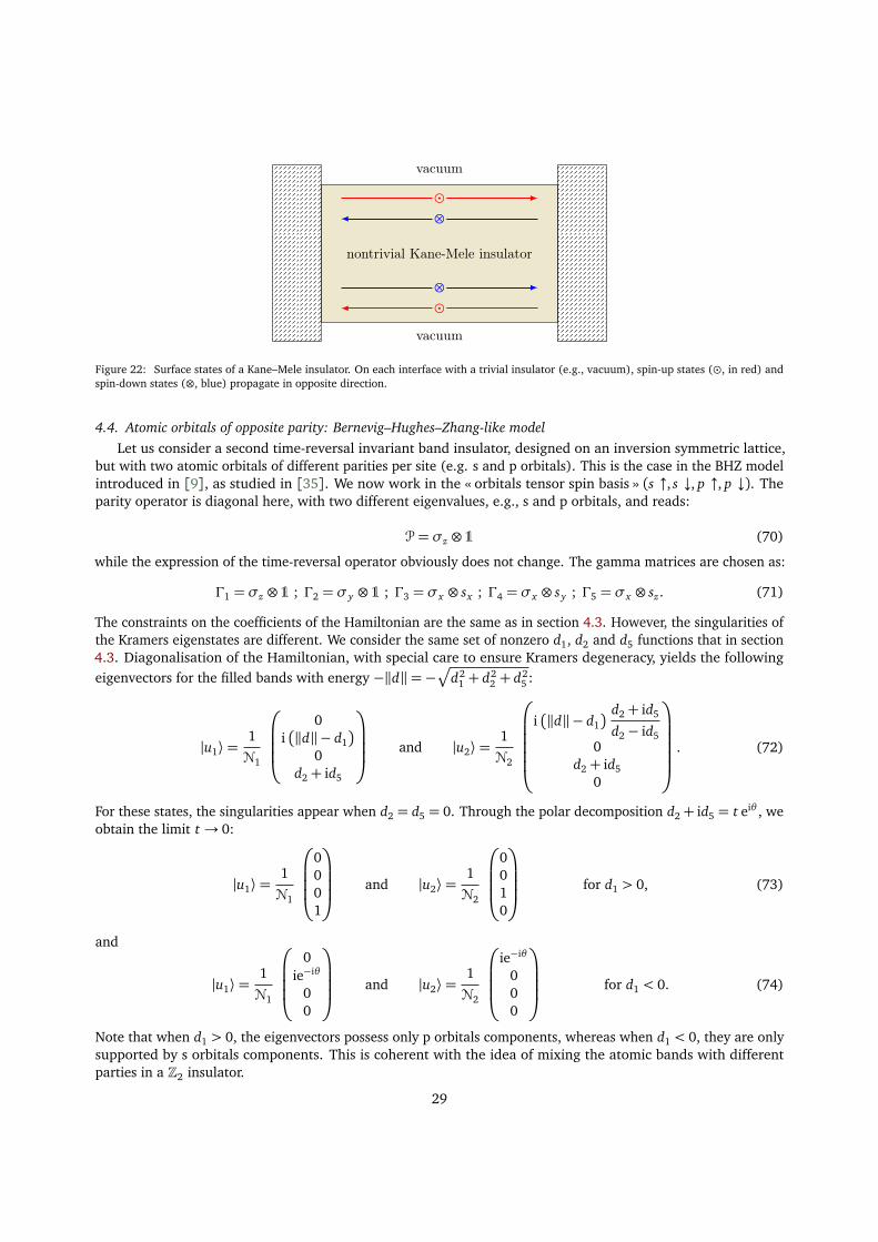
⊙⊗
⊙⊗nontrivial Kane-Mele insulator
vacuum
vacuum
Figure 22: Surface states of a Kane–Mele insulator. On each interface with a trivial insulator (e.g., vacuum), spin-up states (�, in red) andspin-down states (⊗, blue) propagate in opposite direction.
4.4. Atomic orbitals of opposite parity: Bernevig–Hughes–Zhang-like modelLet us consider a second time-reversal invariant band insulator, designed on an inversion symmetric lattice,
but with two atomic orbitals of different parities per site (e.g. s and p orbitals). This is the case in the BHZ modelintroduced in [9], as studied in [35]. We now work in the « orbitals tensor spin basis » (s ↑, s ↓, p ↑, p ↓). Theparity operator is diagonal here, with two different eigenvalues, e.g., s and p orbitals, and reads:
P= σz ⊗1 (70)
while the expression of the time-reversal operator obviously does not change. The gamma matrices are chosen as:
Γ1 = σz ⊗1 ; Γ2 = σy ⊗1 ; Γ3 = σx ⊗ sx ; Γ4 = σx ⊗ sy ; Γ5 = σx ⊗ sz . (71)
The constraints on the coefficients of the Hamiltonian are the same as in section 4.3. However, the singularities ofthe Kramers eigenstates are different. We consider the same set of nonzero d1, d2 and d5 functions that in section4.3. Diagonalisation of the Hamiltonian, with special care to ensure Kramers degeneracy, yields the followingeigenvectors for the filled bands with energy −‖d‖=−
p
d21 + d2
2 + d25 :
|u1⟩=1
N1
0i�
‖d‖− d1�
0d2 + id5
and |u2⟩=1
N2
i�
‖d‖− d1� d2 + id5
d2 − id50
d2 + id50
. (72)
For these states, the singularities appear when d2 = d5 = 0. Through the polar decomposition d2 + id5 = t eiθ , weobtain the limit t → 0:
|u1⟩=1
N1
0001
and |u2⟩=1
N2
0010
for d1 > 0, (73)
and
|u1⟩=1
N1
0ie−iθ
00
and |u2⟩=1
N2
ie−iθ
000
for d1 < 0. (74)
Note that when d1 > 0, the eigenvectors possess only p orbitals components, whereas when d1 < 0, they are onlysupported by s orbitals components. This is coherent with the idea of mixing the atomic bands with differentparties in a Z2 insulator.
29
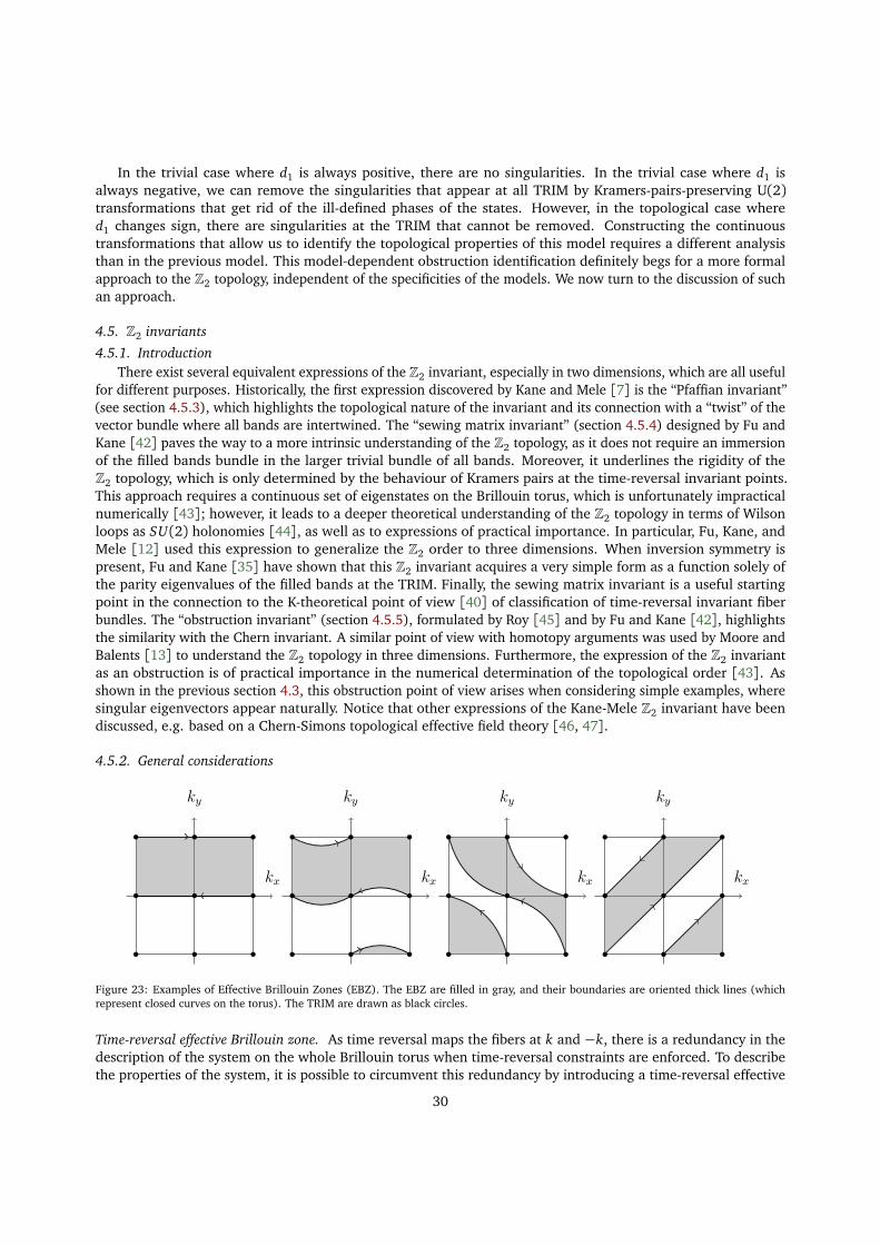
In the trivial case where d1 is always positive, there are no singularities. In the trivial case where d1 isalways negative, we can remove the singularities that appear at all TRIM by Kramers-pairs-preserving U(2)transformations that get rid of the ill-defined phases of the states. However, in the topological case whered1 changes sign, there are singularities at the TRIM that cannot be removed. Constructing the continuoustransformations that allow us to identify the topological properties of this model requires a different analysisthan in the previous model. This model-dependent obstruction identification definitely begs for a more formalapproach to the Z2 topology, independent of the specificities of the models. We now turn to the discussion of suchan approach.
4.5. Z2 invariants
4.5.1. IntroductionThere exist several equivalent expressions of the Z2 invariant, especially in two dimensions, which are all useful
for different purposes. Historically, the first expression discovered by Kane and Mele [7] is the “Pfaffian invariant”(see section 4.5.3), which highlights the topological nature of the invariant and its connection with a “twist” of thevector bundle where all bands are intertwined. The “sewing matrix invariant” (section 4.5.4) designed by Fu andKane [42] paves the way to a more intrinsic understanding of the Z2 topology, as it does not require an immersionof the filled bands bundle in the larger trivial bundle of all bands. Moreover, it underlines the rigidity of theZ2 topology, which is only determined by the behaviour of Kramers pairs at the time-reversal invariant points.This approach requires a continuous set of eigenstates on the Brillouin torus, which is unfortunately impracticalnumerically [43]; however, it leads to a deeper theoretical understanding of the Z2 topology in terms of Wilsonloops as SU(2) holonomies [44], as well as to expressions of practical importance. In particular, Fu, Kane, andMele [12] used this expression to generalize the Z2 order to three dimensions. When inversion symmetry ispresent, Fu and Kane [35] have shown that this Z2 invariant acquires a very simple form as a function solely ofthe parity eigenvalues of the filled bands at the TRIM. Finally, the sewing matrix invariant is a useful startingpoint in the connection to the K-theoretical point of view [40] of classification of time-reversal invariant fiberbundles. The “obstruction invariant” (section 4.5.5), formulated by Roy [45] and by Fu and Kane [42], highlightsthe similarity with the Chern invariant. A similar point of view with homotopy arguments was used by Moore andBalents [13] to understand the Z2 topology in three dimensions. Furthermore, the expression of the Z2 invariantas an obstruction is of practical importance in the numerical determination of the topological order [43]. Asshown in the previous section 4.3, this obstruction point of view arises when considering simple examples, wheresingular eigenvectors appear naturally. Notice that other expressions of the Kane-Mele Z2 invariant have beendiscussed, e.g. based on a Chern-Simons topological effective field theory [46, 47].
4.5.2. General considerations
kx
ky
kx
ky
kx
ky
kx
ky
Figure 23: Examples of Effective Brillouin Zones (EBZ). The EBZ are filled in gray, and their boundaries are oriented thick lines (whichrepresent closed curves on the torus). The TRIM are drawn as black circles.
Time-reversal effective Brillouin zone. As time reversal maps the fibers at k and −k, there is a redundancy in thedescription of the system on the whole Brillouin torus when time-reversal constraints are enforced. To describethe properties of the system, it is possible to circumvent this redundancy by introducing a time-reversal effective
30
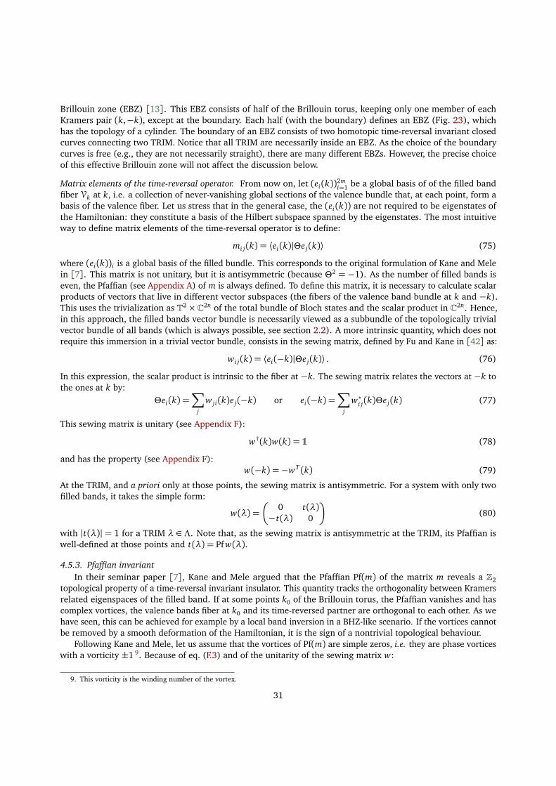
Brillouin zone (EBZ) [13]. This EBZ consists of half of the Brillouin torus, keeping only one member of eachKramers pair (k,−k), except at the boundary. Each half (with the boundary) defines an EBZ (Fig. 23), whichhas the topology of a cylinder. The boundary of an EBZ consists of two homotopic time-reversal invariant closedcurves connecting two TRIM. Notice that all TRIM are necessarily inside an EBZ. As the choice of the boundarycurves is free (e.g., they are not necessarily straight), there are many different EBZs. However, the precise choiceof this effective Brillouin zone will not affect the discussion below.
Matrix elements of the time-reversal operator. From now on, let (ei(k))2mi=1 be a global basis of of the filled band
fiber Vk at k, i.e. a collection of never-vanishing global sections of the valence bundle that, at each point, form abasis of the valence fiber. Let us stress that in the general case, the (ei(k)) are not required to be eigenstates ofthe Hamiltonian: they constitute a basis of the Hilbert subspace spanned by the eigenstates. The most intuitiveway to define matrix elements of the time-reversal operator is to define:
mi j(k) = ⟨ei(k)|Θe j(k)⟩ (75)
where (ei(k))i is a global basis of the filled bundle. This corresponds to the original formulation of Kane and Melein [7]. This matrix is not unitary, but it is antisymmetric (because Θ2 = −1). As the number of filled bands iseven, the Pfaffian (see Appendix A) of m is always defined. To define this matrix, it is necessary to calculate scalarproducts of vectors that live in different vector subspaces (the fibers of the valence band bundle at k and −k).This uses the trivialization as T2 ×C2n of the total bundle of Bloch states and the scalar product in C2n. Hence,in this approach, the filled bands vector bundle is necessarily viewed as a subbundle of the topologically trivialvector bundle of all bands (which is always possible, see section 2.2). A more intrinsic quantity, which does notrequire this immersion in a trivial vector bundle, consists in the sewing matrix, defined by Fu and Kane in [42] as:
wi j(k) = ⟨ei(−k)|Θe j(k)⟩ . (76)
In this expression, the scalar product is intrinsic to the fiber at −k. The sewing matrix relates the vectors at −k tothe ones at k by:
Θei(k) =∑
j
w ji(k)e j(−k) or ei(−k) =∑
j
w?i j(k)Θe j(k) (77)
This sewing matrix is unitary (see Appendix F):
w†(k)w(k) = 1 (78)
and has the property (see Appendix F):w(−k) =−wT (k) (79)
At the TRIM, and a priori only at those points, the sewing matrix is antisymmetric. For a system with only twofilled bands, it takes the simple form:
w(λ) =�
0 t(λ)−t(λ) 0
�
(80)
with |t(λ)| = 1 for a TRIM λ ∈ Λ. Note that, as the sewing matrix is antisymmetric at the TRIM, its Pfaffian iswell-defined at those points and t(λ) = Pf w(λ).
4.5.3. Pfaffian invariantIn their seminar paper [7], Kane and Mele argued that the Pfaffian Pf(m) of the matrix m reveals a Z2
topological property of a time-reversal invariant insulator. This quantity tracks the orthogonality between Kramersrelated eigenspaces of the filled band. If at some points k0 of the Brillouin torus, the Pfaffian vanishes and hascomplex vortices, the valence bands fiber at k0 and its time-reversed partner are orthogonal to each other. As wehave seen, this can be achieved for example by a local band inversion in a BHZ-like scenario. If the vortices cannotbe removed by a smooth deformation of the Hamiltonian, it is the sign of a nontrivial topological behaviour.
Following Kane and Mele, let us assume that the vortices of Pf(m) are simple zeros, i.e. they are phase vorticeswith a vorticity ±1 9. Because of eq. (F.3) and of the unitarity of the sewing matrix w:
9. This vorticity is the winding number of the vortex.
31
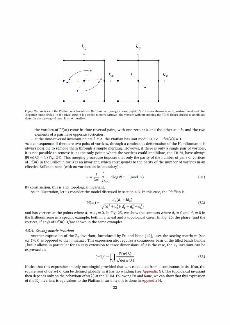
kx
ky
kx
ky
Figure 24: Vortices of the Pfaffian in a trivial case (left) and a topological case (right). Vortices are drawn as red (positive ones) and blue(negative ones) circles. In the trivial case, it is possible to move (arrows) the vortices without crossing the TRIM (black circles) to annihilatethem. In the topological case, it is not possible.
– the vortices of Pf(m) come in time-reversal pairs, with one zero at k and the other at −k, and the twoelements of a pair have opposite vorticities;
– at the time-reversal invariant points λ ∈ Λ, the Pfaffian has unit modulus, i.e. |Pf m(λ)|= 1.As a consequence, if there are two pairs of vortices, through a continuous deformation of the Hamiltonian it isalways possible to remove them through a simple merging. However, if there is only a single pair of vortices,it is not possible to remove it, as the only points where the vortices could annihilate, the TRIM, have always|Pf m(λ)|= 1 (Fig. 24). This merging procedure imposes that only the parity of the number of pairs of vorticesof Pf(m) in the Brillouin torus is an invariant, which corresponds to the parity of the number of vortices in aneffective Brillouin zone (with no vortices on its boundary):
ν =1
2πi
∮
∂ EBZ
d logPf m (mod. 2) (81)
By construction, this is a Z2 topological invariant.As an illustration, let us consider the model discussed in section 4.3. In this case, the Pfaffian is:
Pf(m) =d1 (d1 + id2)
p
(d21 + d2
2 ) (d21 + d2
2 + d25 )
(82)
and has vortices at the points where d1 = d2 = 0. In Fig. 25, we show the contours where d1 = 0 and d2 = 0 inthe Brillouin zone in a specific example, both in a trivial and a topological cases. In Fig. 26, the phase (and thevortices, if any) of Pf(m) is/are shown in the same examples.
4.5.4. Sewing matrix invariantAnother expression of the Z2 invariant, introduced by Fu and Kane [42], uses the sewing matrix w (see
eq. (76)) as opposed to the m matrix . This expression also requires a continuous basis of the filled bands bundle, but it allows in particular for an easy extension to three dimensions. If it is the case, the Z2 invariant can beexpressed as:
(−1)ν =∏
λ∈Λ
Pf w(λ)p
det w(λ)(83)
Notice that this expression in only meaningful provided that w is calculated from a continuous basis. If so, thesquare root of det w(λ) can be defined globally as it has no winding (see Appendix G). The topological invariantthen depends only on the behaviour of w(λ) at the TRIM. Following Fu and Kane, we can show that this expressionof the Z2 invariant is equivalent to the Pfaffian invariant: this is done in Appendix H.
32
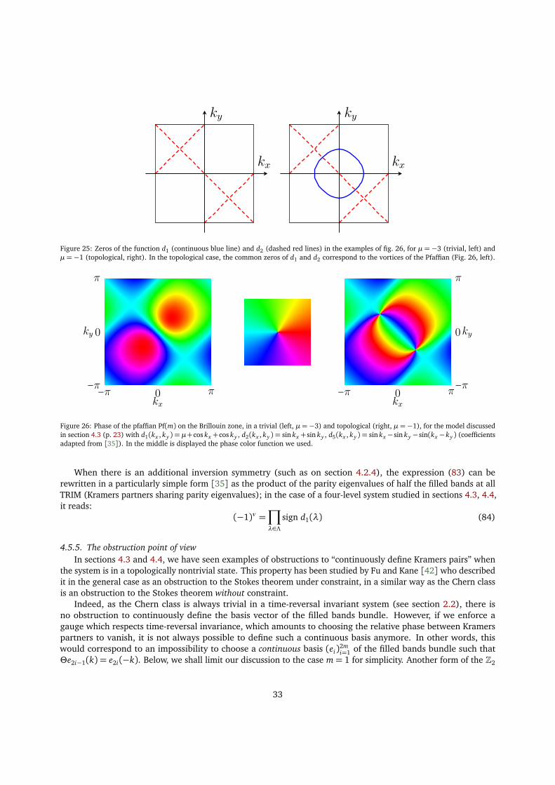
kx
ky
kx
ky
Figure 25: Zeros of the function d1 (continuous blue line) and d2 (dashed red lines) in the examples of fig. 26, for µ=−3 (trivial, left) andµ=−1 (topological, right). In the topological case, the common zeros of d1 and d2 correspond to the vortices of the Pfaffian (Fig. 26, left).
−π
0
π
−π 0 πkx
ky
−π
0
π
−π 0 πkx
ky
Figure 26: Phase of the pfaffian Pf(m) on the Brillouin zone, in a trivial (left, µ =−3) and topological (right, µ =−1), for the model discussedin section 4.3 (p. 23) with d1(kx , ky ) = µ+cos kx +cos ky , d2(kx , ky ) = sin kx +sin ky , d5(kx , ky ) = sin kx −sin ky −sin(kx −ky ) (coefficientsadapted from [35]). In the middle is displayed the phase color function we used.
When there is an additional inversion symmetry (such as on section 4.2.4), the expression (83) can berewritten in a particularly simple form [35] as the product of the parity eigenvalues of half the filled bands at allTRIM (Kramers partners sharing parity eigenvalues); in the case of a four-level system studied in sections 4.3, 4.4,it reads:
(−1)ν =∏
λ∈Λ
sign d1(λ) (84)
4.5.5. The obstruction point of viewIn sections 4.3 and 4.4, we have seen examples of obstructions to “continuously define Kramers pairs” when
the system is in a topologically nontrivial state. This property has been studied by Fu and Kane [42] who describedit in the general case as an obstruction to the Stokes theorem under constraint, in a similar way as the Chern classis an obstruction to the Stokes theorem without constraint.
Indeed, as the Chern class is always trivial in a time-reversal invariant system (see section 2.2), there isno obstruction to continuously define the basis vector of the filled bands bundle. However, if we enforce agauge which respects time-reversal invariance, which amounts to choosing the relative phase between Kramerspartners to vanish, it is not always possible to define such a continuous basis anymore. In other words, thiswould correspond to an impossibility to choose a continuous basis (ei)2m
i=1 of the filled bands bundle such thatΘe2i−1(k) = e2i(−k). Below, we shall limit our discussion to the case m= 1 for simplicity. Another form of the Z2
33
invariant that expresses this point of view is [42]:
ν =1
2π
�∮
∂ EBZ
A−∫
EBZ
F
�
(mod. 2) (85)
where A is the total Berry connection (the sum of the Berry connections of all bands) constructed from Kramerspairs, and F = dA is the Berry curvature. In the trivial case, it is possible to define a continuous basis over theEBZ, the Stokes theorem can be applied, and ν vanishes. However, in the nontrivial case, when ν = 1, there is atopological obstruction to do so.
The equivalence between this expression and the previous ones was demonstrated in [42], and is reviewed in[17, §10.5]. Notice that whereas the Z Chern obstruction is a U(1) obstruction, hence described by a windingnumber, the Z2 obstruction is a SU(2) obstruction, as pointed out by Lee and Ryu [44]. Moore and Balents [13]discuss the obstruction point of view using homotopy theory arguments. They show that the Z2 invariant is a“Chern parity” and generalize it to three dimensions.
4.6. An intrinsic point of view on the Z2 invariant
The aim of this section is to relate the sewing matrix expression (83) of the Z2 invariant to an index recentlyintroduced by Freed and Moore [40]. In doing so, we will gain another interpretation of this Z2 invariant, intrinsicto a fiber bundle with a time-reversal symmetric structure. This point of view uses a type of an orientation onthis fiber bundle over the TRIM’s defined through the introduction of the so-called determinant line bundle. Thedeterminant line bundle possesses over TRIM an oriented real structure. The latter originates from a quaternionicstructure in the valence band bundle imposed by the time-reversal symmetry [48]. The real orientations of thedeterminant bundle at different TRIM are constrained by the topology of the whole time-reversal symmetricvector bundle in a way described by the Kane–Mele invariant.
4.6.1. Quaternionic structure and determinant bundleAt the time-reversal invariant points, the filled bands fiber Vλ is equipped with a quaternionic structure [40].
Indeed, the time-reversal operator Θ acts on this fiber, endowing it with an anti-linear anti-involution that playsthe role of a quaternionic element j = Θ (see Appendix B). With the imaginary unit i, the third quaternionicelement is k= iΘ. The constitutive relations of quaternions are then satisfied: ji= iΘ= k=−Θi=−ji, etc.
From the n-dimensional vector bundle V (with n = 2), we construct the associated determinant bundle asthe nth exterior power ΛnV. By construction, it is a (complex) line bundle on the torus T2. The global basis of Vprovides a global (single element) basis of ΛnV, e.g., for n= 2:
s(k) = e1(k)∧ e2(k) (86)
which is indeed always nonzero. Time-reversal acts on the determinant bundle Λ2V through the operator Λ2Θdefined as:
Λ2Θ : Λ2Vk →Λ2V−k
a ∧ b 7→Θa ∧Θb. (87)
At the TRIM, the operator Λ2Θ, which is anti-linear involutive map from the local fiber onto itself, actssimilarly to a “complex conjugation”, and induces a real structure on the determinant bundle fiber as well as anatural orientation [40]. Indeed, at these TRIM, the filled bands’ fiber Vλ has a quaternionic basis, denoted (e1)(therefore a complex basis (e1,Θe1), as Θe1 is orthogonal to e1), which induces the basis e1 ∧Θe1 of the fiberΛ2Vλ at λ of the determinant bundle Λ2V. This element satisfies:
Λ2Θ�
e1 ∧Θe1�
= e1 ∧Θe1 (88)
and is therefore called a real element of the fiber Λ2Vλ. On the contrary,
Λ2Θ�
i e1 ∧Θe1�
=−ie1 ∧Θe1 (89)
34
is a purely imaginary element. We can define the real part and the imaginary part in the same manner that forcomplex numbers, but with Λ2Θ playing the role of the complex conjugation.
Moreover, we can define a natural orientation for the real elements on this fiber: let us choose by conventione1 ∧Θe1 as a positive element, along with all vectors in Λ2Vλ that are proportional with a positive coefficient. Theelements proportional to this vector with a negative coefficient are called negative elements. These definitions oforientation do not depend on the choice of the quaternionic basis. Indeed, if we consider another element:
f1 = λe1 +µΘe1 (λ et µ ∈ C) (90)
the corresponding element on the determinant fiber reads:
f1 ∧Θ f1 =�
λe1 +µΘe1�
∧Θ�
λe1 +µΘe1�
=�
λe1 +µΘe1�
∧�
λ?Θe1 +µ?ΘΘe1
�
= |λ|2 e1 ∧Θe1 −�
�µ�
�
2Θe1 ∧ e1
=h
|λ|2 +�
�µ�
�
2i
e1 ∧Θe1.
The proportionality coefficient between e1 ∧Θe1 and f1 ∧Θ f1 being real and positive, the choice real element andpositive element (resp. imaginary, negative) deduced from both choices of a basis will be identical: this provides awell-defined natural orientation, and associated real subspace. Note that the natural orientation of the real partof the determinant fiber at the TRIM directly originates from the underlying quaternionic structure of the filledbands fiber.
4.6.2. Kane–Mele invariantLet us consider a nowhere vanishing section σ of the determinant bundle Λ2V previously defined. This section
is said to be time-reversal covariant if:Λ2Θσ(k) = σ(ϑk) (91)
In the following, we will only consider time-reversal covariant sections σ. For a TRIM λ, σ(λ) is a real elementas:
Λ2Θσ(λ) = σ(ϑλ) = σ(λ) (92)
The sign of σ(λ) is therefore well defined. Following Freed and Moore, let us define the following index [40]:
∆=∏
λ∈Λ
sign[σ(λ)], (93)
which will turn out to be the Kane–Mele invariant. Indeed, it takes only values ∆ = ±1 and is a Z2 quantity.Moreover, ∆ can be shown to be independent of the chosen section σ. The demonstration of the invariance of ∆on the chosen section σ is presented in Appendix I.
Moreover, for a carefully chosen section σ, the Freed–Moore Z2 invariant (93) can be expressed as [40]
∆= (−1)ν =∏
λ∈Λ
p
det f (λ)
Pf f (λ), (94)
where the sewing function is defined as the determinant of the sewing matrix (up to a complex conjugation):
f (k) = det w?(k) (95)
The demonstration of this equality is done in Appendix J. The above formulation (94) is nothing but the Fu andKane [42] expression (83) for the Kane–Mele invariant. This demonstrates that the Freed–Moore invariant (93)is indeed another expression of the Kane–Mele Z2 invariant.
35
5. Conclusion
In this introduction to the notion of topological order in insulators, we have discussed the examples of Chernand Z2 Kane–Mele insulators. In a first part, we have studied a simple two-band example of Chern insulator,illustrated by the Haldane model. The occurrence of topological order was shown to manifests itself in anobstruction to define the eigenstates of the fill band in a continuous manner on the Brillouin zone. The indexallowing one to determine the underlying topological nature of an insulator was shown to be the standard firstChern number, whose various expressions were discussed. In the following part, we discussed the Z2 topologicalordering in insulators described by time-reversal symmetric spin 1
2Hamiltonian. To develop a better understanding
of Z2 topological insulators, we have considered two classes of two-dimensional models that account for the Z2topological insulators discovered so far: the Kane–Mele and Bernevig–Hughes–Zhang models. In those examples,we have shown explicitly that, similarly to the case of Chern insulators, an obstruction to define Kramers pairsof states on the Brillouin torus arises in the nontrivial phase of a Z2 insulator. This obstruction consists of pointsingularities of the vectors forming Kramers pairs, which cannot be removed without closing the gap. We arguedthat this obstruction has indeed a topological meaning. These examples provide an intuitive justification of theexpression of the Z2 invariant in an inversion symmetric system, and help us to understand the mechanismunderlying the Z2 topology. We then reviewed the different equivalent expressions of the Z2 invariant.
By choice and for pedagogical reasons, many aspects of this active field have been overlooked. We hope thatthis introduction will be a gateway towards their understanding. We can mention a few directions, includingthe extensions of the notion of topological insulator to three dimensions [12, 13, 14], the topological orderingof various types of superconductors [17, 15, 16, 39], the interplay between topological order and crystallinesymmetries [49] and topological ordering in gapless and interacting phases [50].
Acknowledgments. Our understanding of the subject of this manuscript has enormously benefitted from fruitfuland numerous discussions with our colleague Krzysztof Gawedzki, and we thank him for these as well as hiscareful reading of this manuscript. We also benefitted from interesting discussions with G.-M. Graf about thenotion of obstruction in Z2 topological insulators. This work was supported by an ANR grant Blanc-2010 IsoTop.
Appendix A. Pfaffian of a matrix
The pfaffian Pf(A) of a 2n× 2n skew-symmetric matrix A is the quantity defined by [51]:
Pf A=1
2n n!
∑
σ∈S2n
sign(σ)n∏
i=1
aσ(2i−1),σ(2i) (A.1)
where S2n is the permutation group of 2n elements. The Pfaffian is related to the determinant by (Pf A)2 = det A.For 2× 2 skew-symmetric matrices,
Pf�
0 a−a 0
�
= a (A.2)
Other useful properties of the Pfaffian include Pf(AT) = (−1)n Pf(A), Pf(λA) = λn Pf(A) for λ ∈ C and, for any2n× 2n square matrix B, the identity Pf(B ABT) = det(B) Pf(A).
Appendix B. Quaternionic vector spaces
Appendix B.1. QuaternionsThe quaternion ring H is a division ring (or skew field), built by enhancing the reals with three symbols i, j, k
that satisfy:i2 = j2 = k2 = ijk=−1 (B.1)
so that a generic quaternion readsq = a+ bi+ cj+ dk (B.2)
where a, b, c, d are real. An associative, but noncommutative multiplication on H can be defined, as well as aconjugation where the sign of the symbols i, j, k is reversed, from which a modulus and an inverse can be defined.
36
Appendix B.2. Vector spaces and quaternions
Vector spaces over quaternions are defined naturally. Three points of view on a quaternionic vector space Eare useful [52, 53]:
– E is a n-dimensional quaternionic vector space;– E is a 2n-dimensional complex vector space, endowed with a C-antilinear operation J : E→ E satisfying
J2 =−1 (called a « quaternionic structure map » (see [48]));– E is a 4n-dimensional real vector space endowed with three maps I , J , K satisfying I2 = J2 = K2 =−1 and
I J =−J I = K . Those applications correspond to the multiplication by i, j, and k.Conversely, if one considers a 2n-dimensional complex vector space, a map such as J endows it with a
quaternionic structure [40]. In this case, we call a quaternionic basis an indexed family (ei)i∈I of vectors thatform a basis of E as a quaternionic vector space (i.e. using linear combinations with H-valued coefficients). Thatis to say, we ask (ei , J ei)i∈I to be a basis of E as a complex vector space.
Appendix C. The degree of a map and the winding number
We briefly recall the definitions and properties of the degree of a map [54, 55, 56, 57, 58]. Let us consider a(n− 1)-dimensional, compact, oriented manifold M and an application f from M to the punctured space Rn − p(the space Rn where some point p has been removed), whose image N = f (M) is a n− 1-dimensional compact(thus closed), simply connected in an immersed surface. The natural projection π, defined by:
π : (Rn − p)→ Sn−1
y →y − p
‖y − p‖(C.1)
defines a retractation from Rn − p to Sn−1, and those two spaces are thus homotopically equivalent, i.e. Rn − p 'Sn−1. The pre-image by π of a point a ∈ Sn−1 is the ray ∆(a) coming from p in Rn− p, the point p being excludedfrom ∆(a).
The natural projection π induces a map πN : N → Sn−1, which simply projects the closed surface N on thesphere Sn−1. Hence, π ◦ f : M → Sn−1 is a map between same-dimensional manifolds, and one can thus define itsdegree deg(π ◦ f ) (see [54]) as the “intersection number”, defined from the finite set (π ◦ f )−1({a}) by assigningan orientation number ±1 to each of its points, according to whether π ◦ f preserves (+1) or not (−1) theorientation at this point (that means the orientation number is the sign of the determinant of the tangent map onthis point), and by summing those orientation numbers, the result does not depend on the chosen point a ∈ Sn−1.
In the case considered in this review, this degree is precisely the number of intersection of N with a ray∆(a) = π−1({y}), the orientation number being given by the sign of the scalar product of the radial unit vectorur(∆) with the normal vector at the intersection, and does not depend on the choice of the ray. This amounts todetermining the pre-image (π ◦ f )−1({a}) in two times.
Moreover, two homotopic maps have the same degree, and in the case M → Sn−1 at hand, conversely, twomaps with the same degree are homotopic [54, 55]. As a consequence, the degree of π ◦ f is the homotopy classof the surface N in the homotopy group:
πn−1(Rn − p)' πn−1(Sn−1)' Z (C.2)
that is to say, it is the number of times the surface N warps around the point p (it is the engulfing number, ageneralization of the winding number obtained for n = 2). Often, it appears more useful to consider a givensurface N , and move it with respect to the point p. In the following, we will thus slightly abuse the notationsby calling “degree of f with respect to p” or “degree of N with respect to p” the degree of π ◦ f : M → N (figs.C.27 and C.28). The degree being a homotopy invariant, it can only change when the point p passes through thesurface N (where it is not defined).
37
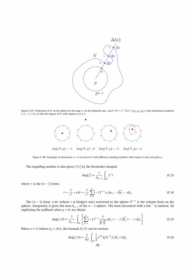
p
Sn−1
∆(a)
a
N
g1
g2
g3
+−+
Figure C.27: Projection of N on the sphere by the map π. In the depicted case, ∆(a)∩ N = π−1(a) =�
g1, g2, g3
, with orientation numbers(+1,−1,+1), so that the degree of N with respect to p is 1.
deg(N,p) = +1deg(N,p) = −1 deg(N,p) = 0 deg(N,p) = 2Figure C.28: Examples in dimension n= 2 of curves N with different winding numbers with respect to the red point p.
The engulfing number is also given [56] by the Kronecker integral:
deg( f ) =1
An−1
∫
M
f ?τ (C.3)
where τ is the (n− 1)-form:
τ=1
rn ? rdr =1
rn
n∑
i=1
(−1)i−1 x i dx1 · · ·ddx j · · ·dxn (C.4)
The (n− 1)-form ?rdr (where ? is Hodge’s star) restricted to the sphere Sn−1 is the volume form on thesphere. Integrated, it gives the area An−1 of the n− 1-sphere. The term decorated with a hat b is omitted. Byexpliciting the pullback when p = 0, we obtain:
deg( f , 0) =1
An−1
∫
M
n∑
j=1
(−1) j−1f j
f
n d f1 ∧ · · · ∧Ód f j ∧ · · · ∧ d fn
(C.5)
When n= 3 (where A2 = 4π), the formula (C.5) can be written:
deg( f , 0) =1
4π
∫
M
1
2εi jk ‖ f ‖−3 fi d f j ∧ d fk. (C.6)
38
If we intepret the term f /‖ f ‖3 as the magnetic field of the monopole located at p = 0 (or, in the general case, atp), the integral on the right-hand side can be seen as the magnetic flux through the surface N .
Appendix D. Winding number in the complex plane
Let us consider a closed curve Γ : S1→ C \ {0} in the complex plane without zero. The winding number of Γcan be expressed [59] as the complex integral:
W[Γ] = deg(Γ, 0) =1
2πi
∫
Γ
dz
z=
1
2πi
∫
Γ
d log z, (D.1)
and W[Γ] ∈ Z is an integer. Now, let us consider a closed curve C on a manifold X , and a continuous complex-valued function f : X → C. We can similarly define the winding number of the curve Γ = f (C) = f ◦C if it doesnot pass through zero.
A n-th root of f exists iff W[ f (C)] ∈ nZ for any closed curve C. Furthermore, a logarithm of f exists iffW[ f (C)] = 0 for any closed curve C, i.e. iff f « has no winding » (see e.g. [60]).
Appendix E. Singular eigenvectors in the Kane–Mele model
In this appendix, we derive the singular behaviours (61a) and (61b) of the eigenstates for the Kane–Melemodel. We obviously have to explicitely include the normalisation when taking the limit t/d5→ 0. By using thesquare root series expansion:
p
1+ (t/d5)2 ' 1+t2
2 d25
, (E.1)
we obtain:
|u1⟩=1
q
t2 +�
�d5
�
�
2 �− sign(d5)− 1− t2/(2 d25 )�2
0�
�d5
�
�
�
− sign(d5)− 1−t2
2 d25
�
0teiθ
. (E.2)
When d5 > 0, the limit t → 0 reads:
|u1(d5 > 0)⟩=1
q
t2 +�
�d5
�
�
2 �−2− t2/(2 d25 )�2
0�
�d5
�
�
�
−2−t2
2 d25
�
0teiθ
→1
Æ
4�
�d5
�
�
2
0−2�
�d5
�
�
00
, (E.3)
whereas for d5 < 0 we have:
|u1(d5 < 0)⟩=1
Æ
1+ t2/(4�
�d5
�
�
2)
0�
�d5
�
�
�
t
2 d25
�
0eiθ
→
000
eiθ
(E.4)
We proceed similarly for |u2⟩.
39
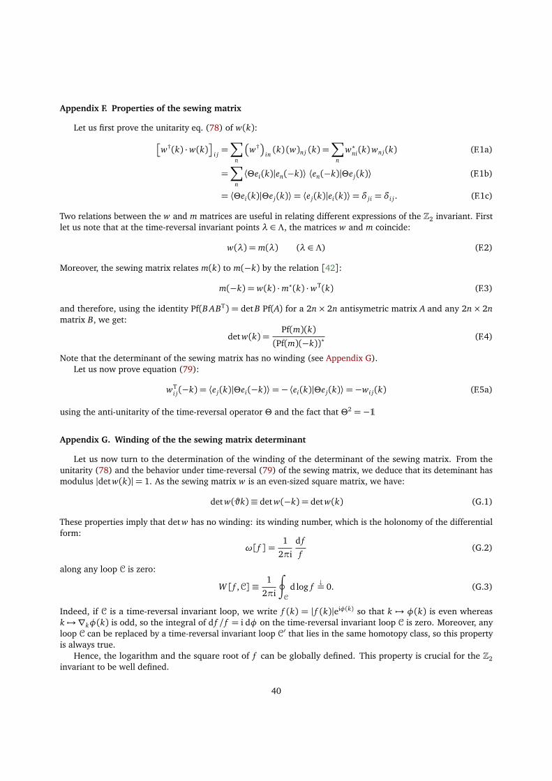
Appendix F. Properties of the sewing matrix
Let us first prove the unitarity eq. (78) of w(k):�
w†(k) ·w(k)�
i j=∑
n
�
w†�
in(k) (w)n j (k) =
∑
n
w?ni(k)wn j(k) (F.1a)
=∑
n
⟨Θei(k)|en(−k)⟩ ⟨en(−k)|Θe j(k)⟩ (F.1b)
= ⟨Θei(k)|Θe j(k)⟩= ⟨e j(k)|ei(k)⟩= δ ji = δi j . (F.1c)
Two relations between the w and m matrices are useful in relating different expressions of the Z2 invariant. Firstlet us note that at the time-reversal invariant points λ ∈ Λ, the matrices w and m coincide:
w(λ) = m(λ) (λ ∈ Λ) (F.2)
Moreover, the sewing matrix relates m(k) to m(−k) by the relation [42]:
m(−k) = w(k) ·m?(k) ·wT(k) (F.3)
and therefore, using the identity Pf(B ABT) = det B Pf(A) for a 2n× 2n antisymetric matrix A and any 2n× 2nmatrix B, we get:
det w(k) =Pf(m)(k)(Pf(m)(−k))?
(F.4)
Note that the determinant of the sewing matrix has no winding (see Appendix G).Let us now prove equation (79):
wTi j(−k) = ⟨e j(k)|Θei(−k)⟩=−⟨ei(k)|Θe j(k)⟩=−wi j(k) (F.5a)
using the anti-unitarity of the time-reversal operator Θ and the fact that Θ2 =−1
Appendix G. Winding of the the sewing matrix determinant
Let us now turn to the determination of the winding of the determinant of the sewing matrix. From theunitarity (78) and the behavior under time-reversal (79) of the sewing matrix, we deduce that its deteminant hasmodulus |det w(k)|= 1. As the sewing matrix w is an even-sized square matrix, we have:
det w(ϑk)≡ det w(−k) = det w(k) (G.1)
These properties imply that det w has no winding: its winding number, which is the holonomy of the differentialform:
ω[ f ] =1
2πi
d f
f(G.2)
along any loop C is zero:
W[ f ,C]≡1
2πi
∮
C
d log f�= 0. (G.3)
Indeed, if C is a time-reversal invariant loop, we write f (k) = | f (k)|eiφ(k) so that k 7→ φ(k) is even whereask 7→ ∇kφ(k) is odd, so the integral of d f / f = i dφ on the time-reversal invariant loop C is zero. Moreover, anyloop C can be replaced by a time-reversal invariant loop C′ that lies in the same homotopy class, so this propertyis always true.
Hence, the logarithm and the square root of f can be globally defined. This property is crucial for the Z2invariant to be well defined.
40
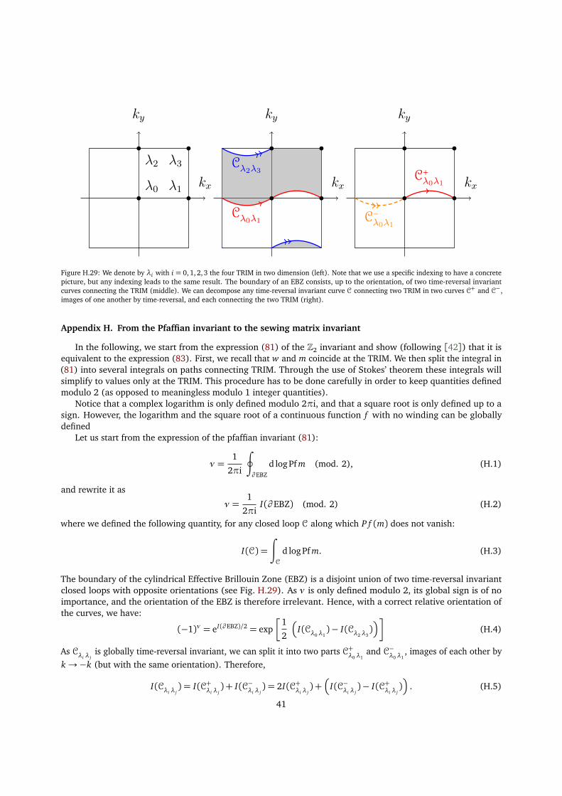
kx
ky
λ0 λ1
λ2 λ3
kx
ky
Cλ0λ1
Cλ2λ3kx
ky
C−λ0λ1
C+λ0λ1
Figure H.29: We denote by λi with i = 0, 1, 2, 3 the four TRIM in two dimension (left). Note that we use a specific indexing to have a concretepicture, but any indexing leads to the same result. The boundary of an EBZ consists, up to the orientation, of two time-reversal invariantcurves connecting the TRIM (middle). We can decompose any time-reversal invariant curve C connecting two TRIM in two curves C+ and C−,images of one another by time-reversal, and each connecting the two TRIM (right).
Appendix H. From the Pfaffian invariant to the sewing matrix invariant
In the following, we start from the expression (81) of the Z2 invariant and show (following [42]) that it isequivalent to the expression (83). First, we recall that w and m coincide at the TRIM. We then split the integral in(81) into several integrals on paths connecting TRIM. Through the use of Stokes’ theorem these integrals willsimplify to values only at the TRIM. This procedure has to be done carefully in order to keep quantities definedmodulo 2 (as opposed to meaningless modulo 1 integer quantities).
Notice that a complex logarithm is only defined modulo 2πi, and that a square root is only defined up to asign. However, the logarithm and the square root of a continuous function f with no winding can be globallydefined
Let us start from the expression of the pfaffian invariant (81):
ν =1
2πi
∮
∂ EBZ
d log Pf m (mod. 2), (H.1)
and rewrite it as
ν =1
2πiI(∂ EBZ) (mod. 2) (H.2)
where we defined the following quantity, for any closed loop C along which P f (m) does not vanish:
I(C) =
∫
C
d logPf m. (H.3)
The boundary of the cylindrical Effective Brillouin Zone (EBZ) is a disjoint union of two time-reversal invariantclosed loops with opposite orientations (see Fig. H.29). As ν is only defined modulo 2, its global sign is of noimportance, and the orientation of the EBZ is therefore irrelevant. Hence, with a correct relative orientation ofthe curves, we have:
(−1)ν = eI(∂ EBZ)/2 = exp�
1
2
�
I(Cλ0 λ1)− I(Cλ2 λ3
)�
�
(H.4)
As Cλi λ jis globally time-reversal invariant, we can split it into two parts C+
λ0 λ1and C−
λ0 λ1, images of each other by
k→−k (but with the same orientation). Therefore,
I(Cλi λ j) = I(C+λi λ j
) + I(C−λi λ j) = 2I(C+λi λ j
) +�
I(C−λi λ j)− I(C+λi λ j
)�
. (H.5)
41
We integrate the first term, and using that at a TRIM λ, m(λ) = w(λ), we get:
exph
I(C+λi λ j)i
= exp
∫
C+λi λ j
d log Pf m(k)
=
Pf m(λ j)
Pf m(λi)=
Pf w(λ j)
Pf w(λi)(H.6)
because ∂ C+λi λ j= λ j − λ j . Using the fact that the two curves C+
λi λ jand C−
λi λ jare images of each other by
time-reversal (up to the orientation), we can write:
I(C+λi λ j)− I(C−λi λ j
) =
∫
C+λi λ j
∇k logPf m(k) · dk−∫
C−λi λ j
∇k logPf m(k) · dk (H.7a)
=
∫
C+λi λ j
∇k�
log Pf m(k) + logPf m(−k)�
· dk (H.7b)
=
∫
C+λi λ j
∇k�
log Pf m(k)− logPf m?(−k)�
· dk (H.7c)
In the last step, we used, via a polar decomposition Pf m(k) = ρ(k) eiθ(k):
log Pf m(k) + Pf m(−k) = 2 logρ(k) + i (θ(k) + θ(−k)) (H.8)
whereaslog Pf m(k)− Pf m?(−k) = i (θ(k) + θ(−k)) . (H.9)
The modulus of a complex number being real, it yields:∫
C+λi λ j
logρ(k) = logρ(λ j)− logρ(λi) = 0 (H.10)
since the Pfaffian has modulus one at the TRIM. From (F.4), we deduce:
log det w(k) = log Pf m(k)− logPf m?(−k) (H.11)
so that, with (H.7) and (H.11),
exp�
1
2
�
I(C+λi λ j)− I(C−λi λ j
)�
�
= exp
1
2
∫
C+λi λ j
d logdet w(k)
=
p
det w(λ j)p
det w(λi)(H.12)
At this stage, it is necessary to continuously define the square root of det w so that the following formula isproperly defined. This is only possible because det w has no winding provided the base vectors are continuouslydefined. Collecting (H.12) and (H.6) into (H.5), we finally obtain:
exp�
1
2I(Cλi λ j
)�
=
p
det w(λi)p
det w(λ j)
Pf w(λ j)
Pf w(λi)=
Pf w(λi)p
det w(λi)
Pf w(λ j)p
det w(λ j)(H.13)
Therefore, the Z2 invariant (H.2) can be written as:
(−1)ν = eI(∂ EBZ)/2 =∏
λ∈Λ
Pf w(λ)p
det w(λ)(H.14)
which is the desired result:
42
Appendix I. Independence from the determinant bundle section of the Z2 Freed–Moore index
In this appendix, following [40], we show the independence of the ∆ index defined in eq. (93) on thechosen section σ. Let us consider two time-reversal covariant nowhere vanishing global sections σ et σ′. As thedeterminant bundle is a line bundle, σ and σ′ are proportional: here is a nowhere vanishing smooth complexfunction j so that:
σ′(k) = j(k)σ(k). (I.1)
Hence,∆′ =
∏
λ∈Λ
sign[σ′(λ)] =∏
λ∈Λ
sign[ j(λ)σ(λ)] =∏
λ∈Λ
sign[ j(λ)]∆. (I.2)
Our purpose is thus to show that:L =
∏
λ∈Λ
sign[ j(λ)] = 1 (I.3)
To proceed, we will rewrite L as the product of two identical holonomies (on homotopic loops). These holonomiescorrespond to the parity of a winding number, and thus take values ±1. However, as there are two identical ones,we obtain J = (±1)2 = 1. We also see that in the most general case, one can change the sign of the product ontwo TRIM, which is therefore not invariant. Let us first deduce that:
j(−k) = j(k)? (I.4)
from the covariance of σ and σ′:
j(−k)σ(−k) = σ′(−k) =Λ2Θσ′(k) =Λ2Θ�
j(k)σ(k)�
j(k)?Λ2Θσ(k) = j(k)?σ(−k). (I.5)
We also note that j(λ) ∈ R, so we have sign j(λ)−1 = sign j(λ) and, with the notations of Appendix H, we have:
L = sign�
j(λ0) j(λ1) j(λ2) j(λ3)�
= sign�
j(λ1)j(λ0)
j(λ3)j(λ2)
�
(I.6)
Let C+λi ,λ j
be a path connecting λi to λ j (see Fig. H.29), and C−λi ,λ j
be its reoriented time reversed version.
Together, C−λi ,λ j
, followed by C+λi ,λ j
, forms a closed loop around the Brillouin torus. We shall write j(k) = ρ(k)eiφ(k)
with ρ(k)> 0 and the real phase φ(k) that may be multivalued on the Brillouin torus. We have:
sign
�
j(λ j)
jλi
�
= ei∫
C+λi ,λ j
dφ(k). (I.7)
On the other hand, by the change of variables k→−k,∫
C+λi ,λ j
dφ(k) =−∫
C−λi ,λ j
dφ(−k), (I.8)
where the overall minus sign is due to reorientation of C−λi ,λ j
as running from λi to λ j . But the symmetry (I.4)implies that dφ(−k) =−dφ(k). Hence:
∫
C+λi ,λ j
dφ(k) =
∫
C−λi ,λ j
dφ(k) =1
2
∫
Cλi ,λ j
dφ(k) = πW[ j,Cλi ,λ j], (I.9)
where W[ j,Cλi ,λ j] is the winding number of j(k) along the loop Cλi ,λ j
. We infer that:
sign
�
j(λ j)
jλi
�
= eiπW[ j,Cλi ,λ j], (I.10)
43
and hence that
sign�
j(λ1)jλ0
j(λ3)j(λ2)
�
= eiπ(W[ j,Cλ0,λ1]+W[ j,Cλ2,λ3
]). (I.11)
The two (integer) winding numbers on the right-hand side are equal as the loops Cλ0,λ1and Cλ2,λ3
on the Brilloinzone are homotopic. Hence the sign in question is +, so that the index (94) does not depend on the choice ofsection σ.
Appendix J. From Freed–Moore to Kane–Mele invariants
We now identify explicitly a global time-reversal covariant section which allows us to identify the Freed–Mooreinvariant (93) with Fu and Kane’s expression of the Z2 invariant. Let us consider the global basis of Λ2V definedby:
s(k) = e1(k)∧ e2(k). (J.1)
As the determinant bundle is a line bundle, Λ2Θs(k) is proportional to s(−k). Let f (k) be the proportionalitycoefficient, so that:
Λ2Θs(k) = f (k) s(−k) (J.2)
We call f the sewing function, for reasons to appear below. By using the expression (77) in terms of the sewingmatrix (76), we obtain:
Λ2Θs(k) = Θe1(k)∧Θe2(k)=�
w11(k)e1(−k) +w21(k)e2(−k)�
∧�
w12(k)e1(−k) +w22(k)e2(−k)�
= w11(k)w22(k) e1(−k)∧ e2(−k) +w21(k)w12(k) e2(−k)∧ e1(−k)=�
w11(k)w22(k)−w12(k)w21(k)�
e1(−k)∧ e2(−k)= det(w) e1(−k)∧ e2(−k). (J.3)
Hence the sewing function appears as the determinant of the sewing matrix (up to a complex conjugation):
f (k) = det w(k) (J.4)
This sewing function has no winding (see Appendix I,Appendix G). We thus consider safely its square root f 1/2.As f (−k) = f (k), we have f 1/2(−k) =± f 1/2(k). Evaluating this expression at the TRIM, the global signs is fixedto be +1. Therefore,
f 1/2(−k) = f 1/2(k). (J.5)
We now define a new section:σ(k) = f 1/2(k)s(k). (J.6)
As | f 1/2(k)|= 1, ( f 1/2(k))? = ( f 1/2(k))−1, it satisfies:
Λ2Θσ(k) = ( f 1/2(k))? Λ2Θs(k) (J.7a)
= ( f 1/2(k))−1 f (k)s(−k) (J.7b)
= f 1/2(k) s(−k) (J.7c)
= f 1/2(−k) s(−k) (J.7d)
= σ(−k) (J.7e)
Let us finally notice that:
e1(λ)∧Θe1(λ) = e1(λ)∧�
w11(λ)e1(ϑλ) +w21(λ)e2(ϑλ)�
(J.8a)
= e1(λ)∧�
w11(λ)e1(λ) +w21(λ)e2(λ)�
(J.8b)
= w21(λ) e1(λ)∧ e2(ϑλ) (J.8c)
=−t(λ) s(λ) (J.8d)
44
where t = w21 = Pf(w) is the Pfaffian of the sewing matrix, which is defined at the TRIM (see (80)). Hence,
σ(λ)≡ f 1/2(λ)s(λ) =−f 1/2(λ)
t(λ)e1(λ)∧Θe1(λ) (J.9)
Using equations (80) and (J.4), we obtain:
[t(λ)]2 = [Pf w(λ)]2 = det w(λ) = f (λ) (J.10)
so we have f 1/2(λ)/t(λ) =±1. Thereby, the ratio f 1/2(λ)/t(λ) gives the sign of the global time-reversal covariantsection σ at the TRIM λ ∈ Λ (up to the overall minus sign).
At a TRIM λ, σ(λ) is a real element whose sign is unambiguously determined, here by:
sign[σ(λ)] =− sign
�
f 1/2(λ)t(λ)
�
=−f 1/2(λ)
t(λ)=−
p
det w(λ)
Pf w(λ)(J.11)
When σ is constructed as explained in last paragraph, the Z2 invariant is indeed [40]:
∆= (−1)ν =∏
λ∈Λ
p
det w(λ)
Pf w(λ)(J.12)
This is obviously equivalent to the Fu and Kane [42] expression (83).[1] M. Nakahara, Geometry, Topology and Physics, Second Edition, 2 ed., Taylor & Francis, 2003.[2] K. v. Klitzing, G. Dorda, M. Pepper, New method for high-accuracy determination of the fine-structure constant based on quantized Hall
resistance, Phys. Rev. Lett. 45 (1980) 494–497. doi:10.1103/PhysRevLett.45.494.[3] B. Douçot, B. Duplantier, V. Pasquier, V. Rivasseau (Eds.), The Quantum Hall Effect, Poincaré Seminar, Birkhäuser, 2004.[4] D. J. Thouless, M. Kohmoto, M. P. Nightingale, M. den Nijs, Quantized Hall conductance in a two-dimensional periodic potential, Phys.
Rev. Lett. 49 (1982) 405–408. doi:10.1103/PhysRevLett.49.405.[5] F. D. M. Haldane, Model for a quantum Hall effect without landau levels: Condensed-matter realization of the "parity anomaly", Phys.
Rev. Lett. 61 (1988) 2015–2018. doi:10.1103/PhysRevLett.61.2015.[6] C.-Z. Chang, J. Zhang, X. Feng, J. Shen, Z. Zhang, M. Guo, K. Li, Y. Ou, P. Wei, L.-L. Wang, Z.-Q. Ji, Y. Feng, S. Ji, X. Chen, J. Jia, X. Dai,
Z. Fang, S.-C. Zhang, K. He, Y. Wang, L. Lu, X.-C. Ma, Q.-K. Xue, Experimental observation of the quantum anomalous Hall effect in amagnetic topological insulator, Science 340 (2013) 167–170. doi:10.1126/science.1234414.
[7] C. L. Kane, E. J. Mele, Z2 topological order and the quantum spin Hall effect, Phys. Rev. Lett. 95 (2005) 146802. doi:10.1103/PhysRevLett.95.146802. arXiv:cond-mat/0506581.
[8] C. L. Kane, E. J. Mele, Quantum spin hall effect in graphene, Phys. Rev. Lett. 95 (2005) 226801. doi:10.1103/PhysRevLett.95.226801. arXiv:cond-mat/0411737.
[9] B. A. Bernevig, T. L. Hughes, S.-C. Zhang, Quantum Spin Hall Effect and Topological Phase Transition in HgTe Quantum Wells, Science314 (2006) 1757–1761. doi:10.1126/science.1133734. arXiv:cond-mat/0611399.
[10] M. König, S. Wiedmann, C. Brüne, A. Roth, H. Buhmann, L. W. Molenkamp, X.-L. Qi, S.-C. Zhang, Quantum spin Hall insulator state inHgTe quantum wells, Science 318 (2007) 766–770. doi:10.1126/science.1148047. arXiv:0710.0582.
[11] A. Roth, C. Brüne, H. Buhmann, L. W. Molenkamp, J. Maciejko, X.-L. Qi, S.-C. Zhang, Nonlocal transport in the quantum spin Hall state,Science 325 (2009) 294. doi:10.1126/science.1174736. arXiv:0905.0365.
[12] L. Fu, C. L. Kane, E. J. Mele, Topological insulators in three dimensions, Phys. Rev. Lett. 98 (2007) 106803. doi:10.1103/PhysRevLett.98.106803. arXiv:cond-mat/0607699.
[13] J. E. Moore, L. Balents, Topological invariants of time-reversal-invariant band structures, Phys. Rev. B 75 (2007) 121306. doi:10.1103/PhysRevB.75.121306. arXiv:cond-mat/0607314.
[14] R. Roy, Topological phases and the quantum spin hall effect in three dimensions, Phys. Rev. B 79 (2009) 195322. doi:10.1103/PhysRevB.79.195322. arXiv:cond-mat/0607531.
[15] M. Z. Hasan, C. L. Kane, Colloquium: Topological insulators, Rev. Mod. Phys. 82 (2010) 3045–3067. doi:10.1103/RevModPhys.82.3045. arXiv:1002.3895.
[16] X.-L. Qi, S.-C. Zhang, Topological insulators and superconductors, Rev. Mod. Phys. 83 (2011) 1057. doi:10.1103/RevModPhys.83.1057. arXiv:1008.2026.
[17] B. A. Bernevig, T. L. Hughes, Topological Insulators and Topological Superconductors, Princeton University Press, 2013.[18] G. E. Volovik, The Universe in a Helium Droplet, Oxford University Press, 2003.[19] X.-G. Wen, Quantum field theory of many-body systems, Oxford University Press, 2004.[20] J. C. Baez, J. P. Muniain, Gauge Fields, Knots, and Gravity, World Scientific, 1994.[21] A. Hatcher, Vector bundles and K-theory, 2003. URL: http://www.math.cornell.edu/~hatcher/VBKT/VBpage.html.[22] B. Simon, Holonomy, the quantum adiabatic theorem, and Berry’s phase, Phys. Rev. Lett. 51 (1983) 2167–2170. doi:10.1103/
PhysRevLett.51.2167.
45
[23] G. Panati, Triviality of bloch and bloch-dirac bundles, Ann. H. Poincaré 8 (2007) 995–1011. doi:10.1007/s00023-007-0326-8.arXiv:math-ph/0601034.
[24] C. Bena, G. Montambaux, Remarks on the tight-binding model of graphene, New Journal of Physics 11 (2009) 095003. doi:10.1088/1367-2630/11/9/095003. arXiv:0712.0765.
[25] J. E. Avron, R. Seiler, B. Simon, Homotopy and Quantization in Condensed Matter Physics, Phys. Rev. Lett. 51 (1983) 51–53.doi:10.1103/PhysRevLett.51.51.
[26] P. A. M. Dirac, Quantised singularities in the electromagnetic field, Proceedings of the Royal Society of London. Series A, ContainingPapers of a Mathematical and Physical Character 133 (1931) pp. 60–72.
[27] D. Chruscinski, A. Jamiołkowski, Geometric Phases in Classical and Quantum Mechanics, Progress in Mathematical Physics, Birkhäuser,2004.
[28] M. V. Berry, Quantal phase factors accompanying adiabatic changes, Proceedings of the Royal Society of London. A. Mathematical andPhysical Sciences 392 (1984) 45–57. doi:10.1098/rspa.1984.0023.
[29] D. Sticlet, F. Piéchon, J.-N. Fuchs, P. Kalugin, P. Simon, Geometrical engineering of a two-band chern insulator in two dimensions witharbitrary topological index, Phys. Rev. B 85 (2012) 165456. doi:10.1103/PhysRevB.85.165456. arXiv:1201.6613.
[30] E. Fradkin, Field Theories of Condensed Matter Physics, 2 ed., Cambridge University Press, 2013.[31] H. B. Nielsen, M. Ninomiya, No go theorem for regularizing chiral fermions, Phys. Lett. 105 (1981) 219. doi:http://dx.doi.org/
10.1016/0370-2693(81)91026-1.[32] M. Le Bellac, Quantum Physics, Cambridge University Press, 2012.[33] J. J. Sakurai, Modern Quantum Mechanics, 1 ed., Addison Wesley, 1993.[34] O. Madelung, Introduction to Solid-State Theory, Springer Series in Solid-State Sciences, Springer, 1996.[35] L. Fu, C. L. Kane, Topological insulators with inversion symmetry, Phys. Rev. B 76 (2007) 045302. doi:10.1103/PhysRevB.76.
045302. arXiv:cond-mat/0611341.[36] G. M. Graf, M. Porta, Bulk-edge correspondence for two-dimensional topological insulators, 2012. arXiv:1207.5989v2.[37] A. Alexandradinata, X. Dai, B. A. Bernevig, Wilson-loop characterization of inversion-symmetric topological insulators, 2012.
arXiv:1208.4234.[38] A. Kitaev, Periodic table for topological insulators and superconductors, in: V. Lebedev, M. Feigel’Man (Eds.), American Institute of
Physics Conference Series, volume 1134 of American Institute of Physics Conference Series, 2009, pp. 22–30. doi:10.1063/1.3149495.arXiv:0901.2686.
[39] S. Ryu, A. P. Schnyder, A. Furusaki, A. W. W. Ludwig, Topological insulators and superconductors: tenfold way and dimensional hierarchy,New Journal of Physics 12 (2010) 065010. doi:10.1088/1367-2630/12/6/065010. arXiv:0912.2157.
[40] D. S. Freed, G. W. Moore, Twisted equivariant matter, Ann. H. Poincaré (2013) 1–97. doi:10.1007/s00023-013-0236-x.arXiv:1208.5055.
[41] R. Jackiw, C. Rebbi, Solitons with fermion number 1/2, Phys. Rev. D 13 (1976) 3398–3409. doi:10.1103/PhysRevD.13.3398.[42] L. Fu, C. L. Kane, Time reversal polarization and a Z2 adiabatic spin pump, Phys. Rev. B 74 (2006) 195312. doi:10.1103/PhysRevB.
74.195312. arXiv:cond-mat/0606336.[43] A. A. Soluyanov, D. Vanderbilt, Wannier representation of Z2 topological insulators, Phys. Rev. B 83 (2011) 035108. doi:10.1103/
PhysRevB.83.035108. arXiv:1009.1415.[44] S.-S. Lee, S. Ryu, Many-body generalization of the z2 topological invariant for the quantum spin Hall effect, Phys. Rev. Lett. 100 (2008)
186807. doi:10.1103/PhysRevLett.100.186807. arXiv:0708.1639.[45] R. Roy, Z2 classification of quantum spin Hall systems: An approach using time-reversal invariance, Phys. Rev. B 79 (2009) 195321.
doi:10.1103/PhysRevB.79.195321. arXiv:cond-mat/0604211.[46] X.-L. Qi, T. L. Hughes, S.-C. Zhang, Topological field theory of time-reversal invariant insulators, Phys. Rev. B 78 (2008) 195424.
doi:10.1103/PhysRevB.78.195424. arXiv:0802.3537.[47] Z. Wang, X.-L. Qi, S.-C. Zhang, Equivalent topological invariants of topological insulators, New Journal of Physics 12 (2010) 065007.
doi:doi:10.1088/1367-2630/12/6/065007. arXiv:0910.5954.[48] J. E. Avron, L. Sadun, J. Segert, B. Simon, Chern numbers, quaternions, and Berry’s phases in Fermi systems, Comm. Math. Phys. 124
(1989) 595–627. doi:10.1007/BF01218452.[49] L. Fu, Topological crystalline insulators, Phys. Rev. Lett. 106 (2011) 106802. doi:10.1103/PhysRevLett.106.106802.
arXiv:1010.1802.[50] A. M. Turner, A. Vishwanath, Beyond band insulators: Topology of semi-metals and interacting phases, 2013. arXiv:1301.0330.[51] N. Bourbaki, Algèbre : Chapitre 9, 1 ed., Springer, 2006.[52] J. H. B. Lawson, The Theory of Gauge Fields in Four Dimensions, American Mathematical Society, 1985.[53] R. W. R. Darling, Differential Forms and Connections, Cambridge University Press, 1994.[54] V. Guillemin, A. Pollack, Differential Topology, reprint (2010) ed., American Mathematical Society, 1974.[55] B. Dubrovin, A. Fomenko, S. Novikov, Modern Geometry - Methods and Applications: Part II: The Geometry and Topology of Manifolds,
1985 ed., Springer, 1985.[56] H. Flanders, Differential forms with applications to the physical sciences, Mathematics in science and engineering, v. 11, 2ed. ed., New
York, Academic Press, 1989.[57] G. Dinca, J. Mawhin, Brouwer Degree and Applications, 2009. URL: http://www.ljll.math.upmc.fr/~smets/ULM/Brouwer_
Degree_and_applications.pdf, to be published.[58] D. Bleecker, B. Booss-Bavnbek, Index Theory with Applications to Mathematics and Physics, 2004. URL: http://milne.ruc.dk/
~Booss/A-S-Index-Book/BlckBss_2012_04_25.pdf, preprint.[59] W. Fulton, Algebraic Topology: A First Course, Springer, 2008.[60] D. Ullrich, Complex Made Simple, Graduate Studies in Mathematics, American Mathematical Society, 2008.
46