© 2022 World Bank

AUTHOR ACCEPTED MANUSCRIPTFINAL PUBLICATION INFORMATION

An Introduction to the IBMR : A Hydro-Economic Model forClimate Change Impact Assessment in Pakistan’s Indus River Basin

The definitive version of the text was subsequently published in

Water International, 38(5), 2013-09-06

Published by Taylor and Francis

THE FINAL PUBLISHED VERSION OF THIS MANUSCRIPTIS AVAILABLE ON THE PUBLISHER’S PLATFORM

This Author Accepted Manuscript is copyrighted by World Bank and published by Taylor and Francis. It is postedhere by agreement between them. Changes resulting from the publishing process—such as editing, corrections,structural formatting, and other quality control mechanisms—may not be reflected in this version of the text.

You may download, copy, and distribute this Author Accepted Manuscript for noncommercial purposes. Your licenseis limited by the following restrictions:

(1) You may use this Author Accepted Manuscript for noncommercial purposes only under a CC BY-NC-ND3.0 IGO license http://creativecommons.org/licenses/by-nc-nd/3.0/igo/.

(2) The integrity of the work and identification of the author, copyright owner, and publisher must be preservedin any copy.

(3) You must attribute this Author Accepted Manuscript in the following format: This is an Author AcceptedManuscript by Yang, Yi-Chen E.; Brown, Casey M.; Yu, Winston H.; Savitsky, Andre An Introduction tothe IBMR : A Hydro-Economic Model for Climate Change Impact Assessment in Pakistan’s Indus RiverBasin © World Bank, published in the Water International38(5) 2013-09-06 CC BY-NC-ND 3.0 IGO http://creativecommons.org/licenses/by-nc-nd/3.0/igo/

1

An Introduction to the IBMR – A Hydro-Economic Model for Climate Change Impact Assessment in Pakistan’s Indus River Basin

Yi-Chen E. Yang1*, Casey M. Brown1, Winston H. Yu2 and Andre Savitsky3

1. Department of Civil and Environmental Engineering, University of Massachusetts – Amherst, yceyang@engin.umass.edu; cbrown@ecs.umass.edu 2. The World Bank, wyu@worldbank.org 3. UZGIP Institute, andresavit@yandex.ru *Corresponding Author Abstract The Indus Basin Model Revised (IBMR) is a hydro-agro-economic optimization model for agricultural investment planning across Pakistan’s Indus Basin provinces. This study describes an update and modification of the model--called IBMR-2012--that reflects the current agro-economic conditions in Pakistan for the purpose of evaluating the impact of climate change on water allocation and food security. Results of hydro-climatic parameter sensitivity and basin-wide and provincial level climate change impacts on crop productions are presented. We show that compared to Punjab, Sindh faces both significantly larger climate change impacts on agriculture and higher uncertainty regarding climate change impacts in the future.

Keywords: Indus Basin Model Revised, Pakistan, water allocation, GCM uncertainty, climate

2

Introduction

Pakistan relies on the largest contiguous irrigation system in the world, known as the

Indus Basin Irrigation System (IBIS), for its basic agricultural production and water supply for

all sectors of the economy. The basin that supports this irrigation system consists of the Indus

River mainstream and its major tributaries--the Kabul, Jhelum, Chenab, Ravi, and Sutlej rivers--

(Figure 1) which flow through four provinces: Khyber Pakhtunkhwa (KPK), Punjab (PUNJAB),

Sindh (SIND) and Balochistan (BLCH) in Pakistan. The basin has two major multi-purpose

storage reservoirs, 19 barrages, 12 inter-river link canals, 45 major irrigation canal commands

(covering over 18 million hectares), and over 120,000 watercourses delivering water to farms

and other productive uses. Annual river flows are about 146 million acre-feet (MAF, 1 MAF

equals 1.234 km3), of which about 106 MAF of water are diverted from the river system to

canals annually (COMSATS, 2003). The total length of the canals is about 60,000 km, with

communal watercourses, farm channels and field ditches running another 1.8 million km. These

canals operate in tandem with vast and growing groundwater extraction from private tubewells.

The IBIS is the backbone of the country’s agricultural economy, and provides 90% of the

food production in the country (Qureshi, 2011). Pakistan’s GDP in 2009 was US $161.819

billion with a contribution by agriculture of 21.5% (WB, 2012). Seventy percent of the country’s

export earnings and 54% of labor force employment occur are within IBIS (Yu et al, 2013). The

intensity of local and regional conflicts over water availability are constantly increasing due to

population growth and increasing water demands (Kahlown and Majeed, 2003).

Duloy and O’Mara (1984) developed the first version of the Indus Basin Model (IBM) as

a research tool for investigating water-related projects and agricultural policies in IBIS. A more

streamlined version of the IBMR model (‘R’ was added for “revised”) was developed in 1988 by

the World Bank’s Development Research Center and the Water and Power Development

Authority (WAPDA) of Pakistan. The IBMR uses the General Algebraic Modeling System

(GAMS) to solve the water allocation for IBIS with a linear or non-linear format (Ahmad et al,

1990). The World Bank and WAPDA updated IBMR in 2002 using 1999-2000 input data, and,

at that time, they updated the modeling structure to incorporate the 1991 Inter-provincial Water

Allocation Accord signed by the four provinces.

Several recent studies, notably the World Bank study Pakistan’s Water Economy:

Running Dry (Briscoe and Qamar, 2006), have focused global attention on Indus water resource

3

issues. To assess the impacts of climate risks and alternative climate change adaptation options

on water and agricultural production in the basin, the World Bank and WAPDA found it

necessary to further update the IBMR. Particularly, the new update aims at analyzing the inter-

relationships among climate, water, and agriculture in Pakistan. A better understanding of these

linkages will help to guide the prioritization and planning of future investments in these sectors.

This paper presents the latest updates of the IBMR using the 2008-2009 hydrologic and

production year as the baseline (named IBMR-2012). The paper then proceeds with hydro-

climatic sensitivity analyses to assess which model parameters as well as which Pakistan

provinces are most sensitive to climate change. The following sections describe the modified

model structure, new input data, and sensitivity analyses of hydro-climate related parameters as

well as results of climate change impact assessment.

Literature Review on Indus Basin Modeling

This study follows a long legacy of research and planning for the Indus Basin in Pakistan.

The first version of the Indus Basin Model, developed by Duloy and O’Mara (1984), included

farm production functions for different cropping technologies in the canal command areas and

was based on a detailed rural household survey conducted in 1978. The analysis also linked

hydrologic inflows and routing with irrigation systems, and thereby showed where efficiencies

could be gained in water allocation.

WAPDA started the next major basin analysis, known as the Water Sector Investment

Planning Study (WSIPS), in the late 1980s and focused on mid-term (10 year) development

alternatives (WAPDA, 1990). This study drew upon a farm survey in 1988 to update farm

production technologies and functions by canal command in the IBMR. The WSIPS used the

model to evaluate a range of investment portfolios: no change, minimum investment, a basic plan

(75 billion Pakistan Rs.) that optimized net economic profits subject to a capital constraint, and a

maximum plan if additional investment funds were available. A detailed guide to the IBMR was

written by Ahmad et al. (1990). Ahmad and Kutcher (1992) applied this IBMR and evaluated

environmental (surface water and groundwater, both fresh and saline) considerations of different

irrigation plans. This study noted the following emerging water and food challenges in their

report: slowing crop yield growth, increasing water scarcity, deteriorating infrastructure,

extensive waterlogging and salinity, and the high cost of drainage for canal command areas.

4

They also used the IBMR to examine the sources of salinity in groundwater and buildup in soils

after optimized water allocation under varied water management policies. Various projects and

programs later used the IBMR to show, for example, the impact of Kalabagh Dam (Ahmad et al,

1986); to assess waterlogging and salinity under different scenarios of crop yields and tubewell

investment levels in Sindh province (Rehman and Rehman, 1993); and to identify salinity

management alternatives for the Rechna Doab region of Punjab (Rehman et al, 1997).

Moreover, a joint WAPDA-U.S. Environmental Protection Agency team used the IBMR

model to study Complex River Basin Management in a Changing Global Climate: A National

Assessment, analyzing General Circulation Model (GCM) climate scenarios along with WAPDA

development alternatives in the late 1980s (Wescoat and Leichenko, 1992). They ran the model

with two different water allocation rules: 100% of historical water allocations (i.e. fixed delivery)

and 80% of historical allocations, assuming that the remainder would be used outside irrigated

agriculture. This early study showed that the impact of climate change can reduce the net

economic profits of the minimum investment plan studied by 40% to 100%. This earlier work

also demonstrated that, with some exceptions, the Indus basin irrigation baseline values seemed

relatively robust under different future climate conditions.

The 2002 IBMR update used 1999-2000 input data for the baseline. This IBMR-2002

was applied to evaluate the effects of raising the Mangla Dam (Alam and Olsthoorn, 2011). As

this literature review shows, the IBMR has been effectively used for critical water-related

investment analysis. A further update of the IBMR, with new input data and an updated

modeling structure (corresponding to the current hydro-agro-economic conditions in Pakistan)

would thus have great potential to help decision-makers understand the impact of climate change

and water governance changes on the agricultural sector in Pakistan.

The IBMR Modeling structure

The IBMR is a hydro-agro-economic model using agro-climatic zones (ACZ, Figure 1)

as basic spatial units. The overall model objective is to maximize the sum of zonal consumer and

producer surpluses (CPS), which are the net economic profits for the entire Indus Basin. The

IBMR-2012 models CPS using a supply-demand relationship. Since CPS has a non-linear format,

the IBMR-2012 uses a piece-wise linear programming approach to solve this objective function.

Although the modeled prices may fluctuate between zero and the intercept of the demand curve,

5

this is unlikely to happen in reality, and so prices are given upper and lower bounds. It is

assumed that, outside of these bounds, inter-zonal trade will exist. However, the model does not

actually simulate such trade. The IBMR also does not consider international trade explicitly but

does account for the prices of international exports and imports and adjusts production

accordingly.

The four provinces currently modeled contain one or more ACZs that represent a

consistent cropping pattern, land characteristics and climatic conditions. The model includes 12

ACZs. A node-link system is used to represent the river (supply node)-canal (demand node)

network, and this node-link system provides surface water to each ACZ. Agricultural production

and consumption is simulated at the ACZ level. Each ACZ consists of one or more canal

command areas (CCAs, Figure 1) based on the canal water diversions. In some cases, one CCA

can contribute water to two ACZs. Therefore, each CCA has been further divided into four

subareas based on the proportion of water provided by canals (Ahmad et al, 1990). This

hierarchal structure of the IBMR-2012 is provided in Table 1.

In the IBMR, the residual moisture in the root zone is explicitly modeled and represents a

potential source of water for crops. Crop water needs are met from precipitation, canals,

groundwater wells (mostly shallow), and soil moisture in the root zone (also known as “sub-

irrigation”). An evaporation parameter in the model is used to define the "sub-irrigation" water

available to plants. The IBMR assumes that 60% of the evaporation from shallow groundwater

can be absorbed by crops (Ahmad et al, 1990 and Ahmad and Kutcher, 1992) and the remainder

is lost as evaporation to the atmosphere. Therefore, although evaporation is a “water loss” from

a water balance perspective, part of that “water loss” from shallow groundwater is used by crops

which are “water gains” from a crop perspective. This water balance at the ACZ level is

graphically depicted in Figure 3. This figure also demonstrates how surface and groundwater

interact.

The IBMR-2012 input and output data and the key equations are described as follows.

Input data

The input data of IBMR-2012 can be categorized as 1) agronomic and livestock data, 2)

economic data, 3) resources inventory, and 4) irrigation systems and water data.

Agronomic and Livestock Data

6

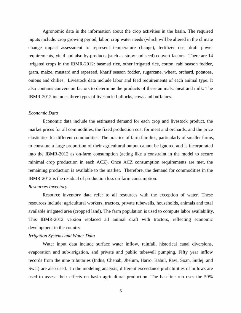
Agronomic data is the information about the crop activities in the basin. The required

inputs include: crop growing period, labor, crop water needs (which will be altered in the climate

change impact assessment to represent temperature change), fertilizer use, draft power

requirements, yield and also by-products (such as straw and seed) convert factors. There are 14

irrigated crops in the IBMR-2012: basmati rice, other irrigated rice, cotton, rabi season fodder,

gram, maize, mustard and rapeseed, kharif season fodder, sugarcane, wheat, orchard, potatoes,

onions and chilies. Livestock data include labor and feed requirements of each animal type. It

also contains conversion factors to determine the products of these animals: meat and milk. The

IBMR-2012 includes three types of livestock: bullocks, cows and buffaloes.

Economic Data

Economic data include the estimated demand for each crop and livestock product, the

market prices for all commodities, the fixed production cost for meat and orchards, and the price

elasticities for different commodities. The practice of farm families, particularly of smaller farms,

to consume a large proportion of their agricultural output cannot be ignored and is incorporated

into the IBMR-2012 as on-farm consumption (acting like a constraint in the model to secure

minimal crop production in each ACZ). Once ACZ consumption requirements are met, the

remaining production is available to the market. Therefore, the demand for commodities in the

IBMR-2012 is the residual of production less on-farm consumption.

Resources Inventory

Resource inventory data refer to all resources with the exception of water. These

resources include: agricultural workers, tractors, private tubewells, households, animals and total

available irrigated area (cropped land). The farm population is used to compute labor availability.

This IBMR-2012 version replaced all animal draft with tractors, reflecting economic

development in the country.

Irrigation Systems and Water Data

Water input data include surface water inflow, rainfall, historical canal diversions,

evaporation and sub-irrigation, and private and public tubewell pumping. Fifty year inflow

records from the nine tributaries (Indus, Chenab, Jhelum, Harro, Kabul, Ravi, Soan, Sutlej, and

Swat) are also used. In the modeling analysis, different exceedance probabilities of inflows are

used to assess their effects on basin agricultural production. The baseline run uses the 50%

7

exceedance probability which equals 132 MAF annually. The total live reservoir storage in the

model is 11.5 MAF. Four reservoirs are used in the current model structure: Mangla, Tarbela,

Chashma and Chotiari. When modeling the irrigation system, the basic unit is the CCA. All data

on these commands are aggregated to the level of the agricultural model (i.e. ACZ).

Equations

In total, 20 equations are used to optimize the complex processes related to water

allocation and economic activities. These equations can be categorized into six classes: 1)

objective function, 2) economic equations, 3) water balance equations, 4) canal equations, 5)

crop equations and 6) livestock equations. Only four critical equations are explained here, others

can be found in Ahmad et al. (1990) and Yu et al. (2013).

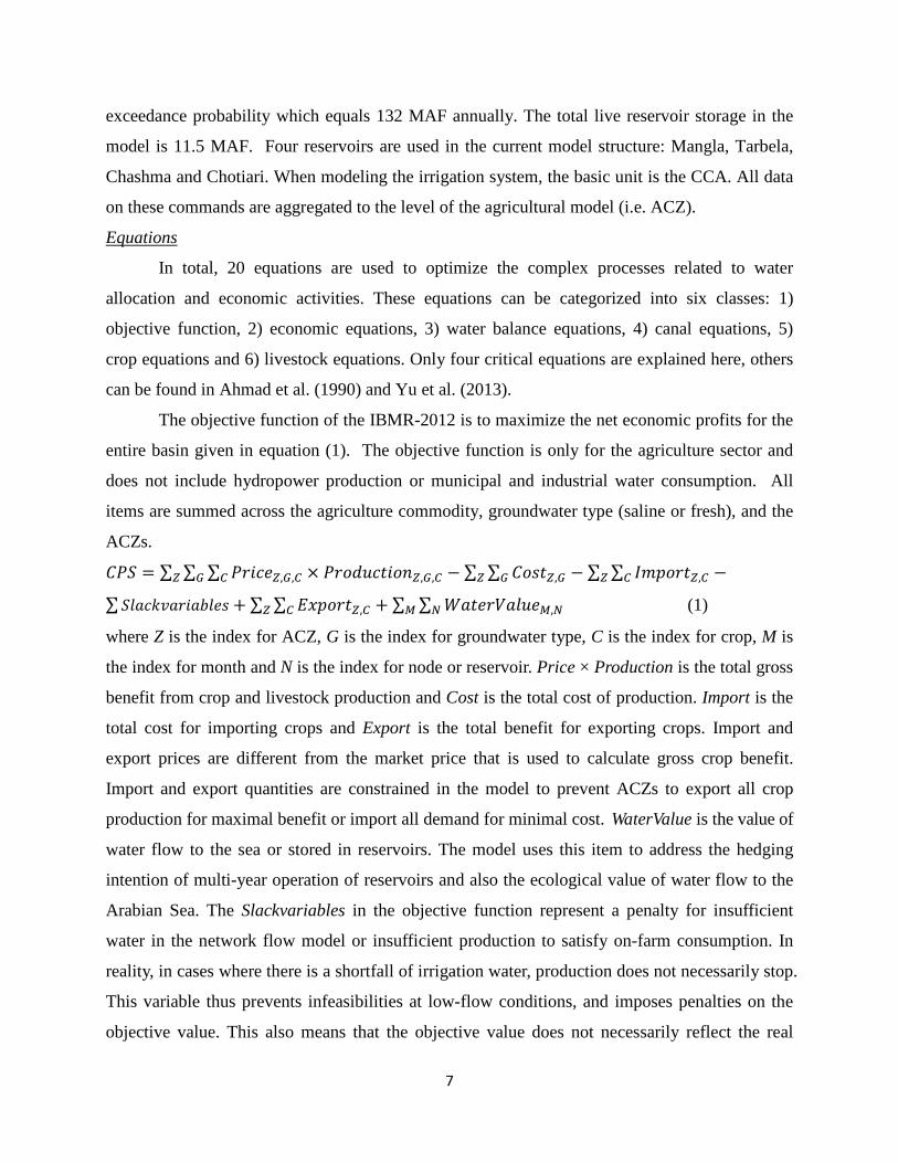
The objective function of the IBMR-2012 is to maximize the net economic profits for the

entire basin given in equation (1). The objective function is only for the agriculture sector and

does not include hydropower production or municipal and industrial water consumption. All

items are summed across the agriculture commodity, groundwater type (saline or fresh), and the

ACZs.

𝐶𝑃𝑆 = ∑ ∑ ∑ 𝑃𝑟𝑖𝑐𝑒𝑍,𝐺,𝐶 × 𝑃𝑟𝑜𝑑𝑢𝑐𝑡𝑖𝑜𝑛𝑍,𝐺,𝐶𝐶𝐺𝑍 − ∑ ∑ 𝐶𝑜𝑠𝑡𝑍,𝐺𝐺𝑍 − ∑ ∑ 𝐼𝑚𝑝𝑜𝑟𝑡𝑍,𝐶𝐶𝑍 −

∑ 𝑆𝑙𝑎𝑐𝑘𝑣𝑎𝑟𝑖𝑎𝑏𝑙𝑒𝑠 + ∑ ∑ 𝐸𝑥𝑝𝑜𝑟𝑡𝑍,𝐶𝐶𝑍 + ∑ ∑ 𝑊𝑎𝑡𝑒𝑟𝑉𝑎𝑙𝑢𝑒𝑀,𝑁𝑁𝑀 (1)

where Z is the index for ACZ, G is the index for groundwater type, C is the index for crop, M is

the index for month and N is the index for node or reservoir. Price × Production is the total gross

benefit from crop and livestock production and Cost is the total cost of production. Import is the

total cost for importing crops and Export is the total benefit for exporting crops. Import and

export prices are different from the market price that is used to calculate gross crop benefit.

Import and export quantities are constrained in the model to prevent ACZs to export all crop

production for maximal benefit or import all demand for minimal cost. WaterValue is the value of

water flow to the sea or stored in reservoirs. The model uses this item to address the hedging

intention of multi-year operation of reservoirs and also the ecological value of water flow to the

Arabian Sea. The Slackvariables in the objective function represent a penalty for insufficient

water in the network flow model or insufficient production to satisfy on-farm consumption. In

reality, in cases where there is a shortfall of irrigation water, production does not necessarily stop.

This variable thus prevents infeasibilities at low-flow conditions, and imposes penalties on the

objective value. This also means that the objective value does not necessarily reflect the real

8

basin-wide net economic profits that would be observed under these water shortfall conditions.

The cost function contains all the costs for crop and livestock production in each ACZ as

shown in equation (2).

𝐶𝑜𝑠𝑡𝑍,𝐺 = ∑ ∑ ∑ ∑ �𝐹𝐸𝑅𝑇𝑍,𝐶,𝑆,𝑀 + 𝑀𝐼𝑆𝐶𝐶𝑇𝑍,𝐶,𝑆,𝑀 + 𝑆𝐸𝐸𝐷𝑃𝑍,𝐶,𝑆,𝑀 + 𝑇𝑊𝑍,𝐶,𝑆,𝑀 +𝑊𝑆𝐶𝑍

𝑇𝑅𝐴𝐶𝑇𝑂𝑅𝑍,𝐶,𝑆,𝑀� + ∑ ∑ ∑ 𝐴𝑛𝑖𝑚𝑎𝑙𝑍,𝐺,𝐴𝐴𝐺𝑍 + ∑ ∑ 𝑃𝑃𝑍,𝑆𝐸𝐴𝑆𝐸𝐴𝑍 + ∑ ∑ ∑ 𝐿𝑎𝑏𝑜𝑟𝑍,𝐺,𝑀𝑀𝐺𝑍 (2)

where S is the index for cropping sequence (e.g. standard, late or early planting), W is the index

for water application (e.g. standard, light or heavy stress while stress application require less

water and labor and produce less output), A is the index for different animals (cow bullock and

buffalo) and SEA is the index for season (rabi and kharif). FERT is the cost of fertilizer, MISCCT

are miscellaneous costs like insecticides and herbicides, SEEDP is the cost of seed, TW is the

energy cost for groundwater pumping, TRACTOR is the cost for operating tractors, Animal is the

fixed cost for livestock, PP is the cost for purchased protein concentrates for animals and Labor

is the cost for hiring labor.

Water balances in the river network and root zone are the essential mass balances in the

IBMR. The surface water balance is related to the river routing process in the IBMR. The

following equation (3) describes the entire river network monthly water balance at each node.

∑ 𝐼𝑛𝑓𝑙𝑜𝑤𝐼𝑀

𝐼 + ∑ 𝑅𝐼𝑉𝐸𝑅𝐷𝑁 × 𝑇𝑅𝐼𝐵𝑁𝑀𝑁 + ∑ 𝑅𝐼𝑉𝐸𝑅𝐶𝑁 × 𝑇𝑅𝐼𝐵𝑁𝑀−1𝑁 + ∑ 𝑅𝐼𝑉𝐸𝑅𝐵𝑁 × 𝐹𝑁𝑀𝑁 +

∑ 𝑅𝐼𝑉𝐸𝑅𝐶𝑁 × 𝐹𝑁𝑀−1𝑁 + ∑ 𝑅𝐶𝑂𝑁𝑇𝑁𝑀−1 − 𝑅𝐶𝑂𝑁𝑇𝑁𝑀 + 𝑃𝑟𝑒𝑐𝑁𝑀 + 𝐸𝑣𝑎𝑝𝑁𝑀𝑁 − ∑ 𝐶𝐴𝑁𝐴𝐿𝐷𝐼𝑉𝑁𝑀𝑁 +

𝑆𝑙𝑎𝑐𝑘𝑊𝑎𝑡𝑒𝑟𝑁𝑀 = 0 (3)

where I is the index for inflow node. Inflow is the streamflow, RIVERD is the routing coefficient

for tributaries, TRIB is the tributaries’ flow, RIVERC is the routing coefficient for the previous

month, RIVERB is the routing coefficient for the mainstream, F is the mainstream flow, RCONT

is the monthly reservoir storage, Prec is the rainfall on the reservoir surface, EVAP is the

evaporation loss from the reservoir surface, CANALDIV is the canal diversion and SlackWater is

the slack surface water (one of the slack variables in the objective function) needed at nodes.

The root zone water balance at each ACZ in IBMR is the relationship between the total

available water in the root zone and the total crop water requirements as shown in Figure 2. The

following equation (4) describes this balance.

𝑀𝑎𝑥��𝑊𝑁𝑅𝑍,𝐺,𝐶,𝑆,𝑊𝑀 − 𝑆𝑈𝐵𝐼𝑅𝑅𝐼𝑍,𝐺

𝑀 ∗ 𝐿𝐴𝑁𝐷𝑍,𝐺,𝐶,𝑆,𝑊𝑀 �, 0� × 𝑋𝑍,𝐺,𝐶,𝑆,𝑊

𝑀 ≤ 𝑇𝑊𝑍,𝐺𝑀 + 𝐺𝑊𝑇𝑍,𝐺

𝑀 +

𝑊𝐷𝐼𝑉𝑅𝑍𝑍,𝐺𝑀 + 𝑆𝑙𝑎𝑐𝑘𝑅𝑊𝑎𝑡𝑒𝑟𝑍,𝐺 (4)

9

where WNR is the water requirement from crops, SUBIRRI is the sub-irrigation, X is the cropped

area, TW is the total private tubewell pumping, GWT is total public tubewell pumping, WDIVRZ

is the surface water diversion and SlackRWater is the slack root zone water, which is one of the

slack variables in the objective function.

Major Constraints

Three major constraints are applied in the IBMR. 1) canal capacity: The physical canal

capacity is used as the upper boundary of canal water diversions in the model. 2) provincial

historical diversion accord: Maintaining the 1991 Inter-provincial Water Allocation Accord is

another constraint in the model. This water sharing agreement specifies how much water needs

to be delivered to each province. In order to consider this accord in the IBMR-2012, the actual

monthly canal diversions from 1991 to 2000 (after the Accord) are averaged and utilized as the

constraint itself (“DIVACRD”). In this study, a 20% deviation from the monthly canal diversion

was allowed, that is, each canal command diversion can range from 0.8–1.2 times the historical,

long-term average value (while maintaining the physical constraints in the system). This is the

same setting followed by WAPDA (1990). 3) reservoir operation rule: No complex operation

rules have been applied to these reservoirs. Monthly upper and lower boundaries of reservoir

storage are the only constraints. This is acceptable given that the model operates on a single-year

basis. This constraint affects surface water routing and avoids reservoir drawdown to nil at the

end of the year.

Output data

The output data from the IBMR contains a great deal of information. The first output is

values in the objective function. Key outputs include gross profit from agricultural production,

farm cost, agricultural imports and exports, the economic value of water in reservoirs and the

flow to the sea. The slack values can also be assessed. Non-zero slack values signify water stress

in the model run. Cropped areas of different crops in each ACZ are one of the major agricultural

outputs. The model provides detailed information for every combination of cropping sequence

and water application of crop outputs. For example, production can be summed across ACZs or

provinces or from seasonal to annual. The results are also provided for each ACZ with different

groundwater types (fresh and saline). Resources used, such as labor and fertilizer (both quantity

and cost), are also calculated for each ACZ. Hydropower generation from reservoirs is a by-

10

product from the model. The final major output from the IBMR-2012 is the surface water and

groundwater balance for each ACZ.

Model baseline and climate change impact settings

Model baseline and diagnosis

The baseline setting uses the agronomic, economic and resources inventory input data

from 2008 to 2009. The 50% exceedance probability is used as inflow and long-term average

rainfall and crop water requirements as hydro-climatic inputs. This section presents the baseline

performance of the IBMR. Table 2 shows the major outputs from the model. The basin-wide

net profit from agriculture is 2,850,099 million PRs. (USD $35.62 billion where 1 USD = 80 PRs.

in 2009). Punjab has the largest cropped area, production and profit, followed by Sindh. Surface

and groundwater use across the provinces follows the 1991 Accord closely. Punjab diverts 59.9

MAF, Sindh diverts 44.1 MAF and other provinces divert 8.4 MAF. Punjab uses most

groundwater, at about 53.2 MAF. Basmati rice, cotton, sugarcane and wheat generate the highest

gross profit in Punjab. Other irrigated rice and cotton gross profit are highest in Sindh (Table 3).

The primary production costs are hired labor, and tractor and fertilizer use (Table 4).

Given the complexity of the IBMR-2012 and the assumptions that it requires, we evaluate

the model performance to increase confidence in the results of the simulations. The basin-wide

net economic profits (USD $35.62 billion) is very close to Pakistan’s agricultural GDP in 2009:

USD $34.79 billion according to the World Development Indicators (WB, 2012). The

government report “Agricultural Statistics of Pakistan 2008-2009” (MINFA, 2010) was used to

compare the provincial level results. The results from IBMR-2012 are not expected to exactly

match the observed values reported in MINFA (2010). The purpose of this comparison is to

evaluate the ability of the model to provide a realistic representation of the hydro-agro-economic

system. The primary agro-economic outputs of the IBMR, such as cropped area and crop

production at the provincial level, were compared with observed values. Since KPK and BLCH

cover a smaller proportion of the Indus River Basin, only Punjab and Sindh were selected for the

comparison.

The coefficients of determination (R2) of cropped areas among 14 crops between the

IBMR baseline run and MINFA data for 2009 were 0.98 for both Punjab and Sindh. The total

cropped area in Punjab is 32.38 million acres from the IBMR while MINFA data show 33.84

11

million acres in 2009 and the root mean-square-error (RMSE) is 0.95 million acres. The total

cropped area in Sindh is 8.13 million acres from the IBMR while MINFA data show 7.06 million

acres in 2009 and the RMSE is 0.63 million acres. The R2 of crop production among 14 crops are

0.99 for both Punjab and Sindh. Crop production in Punjab is 65.37 and 73.42 million tons in the

IBMR and the MINFA data, respectively. Crop production in Sindh is 24.91 and 23.84 million

tons in the IBMR and the MINFA data, respectively. RMSEs for crop production are 1.97 and

0.76 million tons in Punjab and Sindh, respectively. These results show that the model represents

cropped area and production well. Although the absolute values might be different, the relative

cropped pattern (proportion of each crop in area and production) are similar to the observations.

Climate change impact setting

Liniger et al. (1998) suggested that 90% of the lowland flow of the Indus River originates

from the western Himalaya mountain areas. However, several studies have shown that this

region might have a different response to the impact of climate change compared to other regions

in the world (Archer, 2003; Flowler and Archer, 2006; Kaab et al., 2012). Most of the studies

point to a generally increasing annual temperature trend (based on historical data); however, for,

the changes in precipitation, the studies show diverging trends. The uncertainty of future climate

predictions (temperature and precipitation) will significantly affect the prediction of streamflow

in the Indus River. Different studies predict different percentages of snow and glacier melt

contribution (less than 40% to more than 60%) to the streamflow of the Upper Indus Basin (UIB)

(Bookhagen and Burbank, 2010; Jeelani et al., 2012). Glacier-melt dominated rivers will be

affected more by spring and summer temperature increase and snow melt dominated rivers will

be affected more by winter precipitation and summer temperature. Combing all these

uncertainties together, different studies suggest varying streamflow changes in the future. Akhtar

et al. (2008) suggest an increasing trend in summer flows from the UIB under the SRES A2

scenario; with a 1oC increase in temperature resulting in a 16%-increase in streamflow. Tahir et

al. (2011) offered a similar conclusion but with a different magnitude (1oC increase in

temperature would result in a 33%-increase in streamflow). However, Immerzeel et al. (2010)

showed decreasing summer flows in the Indus under the A1B scenario for 2046-2065 period.

Due to the large uncertainty about climate change impacts, this study applies the method

proposed by Brown and Wilby (2012) that systematically evaluates the system’s response (in our

case: the Indus Basin Irrigation System) under a much wider range of future climate conditions.

12

This process is named the “climate response surface” construction. After the “climate response

surface” has been created, we overlap 17 GCM (SRES A2 and A1B scenarios) used in Global

Change Impact Study Centre reports (Islam et al., 2009a and 2009b) to evaluate the uncertainty

from GCM predictions. By overlapping GCM projections with climate response surfaces, this

method can visualize the GCM uncertainty and demonstrate the robustness of the system

response to climate information.

Results and discussion

Sensitivities of hydro-climate related parameters

Conducting sensitivities of hydro-climate related parameters is critical for climate change impact

assessment since the IBMR-2012 is not a physically-based model which can directly use future

climate input (temperature and precipitation from GCMs) for modeling results. We test several

hydro-climate related parameters in this section.

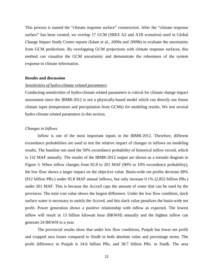
Changes in Inflows

Inflow is one of the most important inputs in the IBMR-2012. Therefore, different

exceedance probabilities are used to test the relative impact of changes in inflows on modeling

results. The baseline run used the 50% exceedance probability of historical inflow record, which

is 132 MAF annually. The results of the IBMR-2012 output are shown as a tornado diagram in

Figure 3. When inflow changes from 92.8 to 201 MAF (90% to 10% exceedance probability),

the low flow shows a larger impact on the objective value. Basin-wide net profits decrease 68%

(912 billion PRs.) under 92.8 MAF annual inflows, but only increase 0.1% (2,852 billion PRs.)

under 201 MAF. This is because the Accord caps the amount of water that can be used by the

provinces. The total cost value shows the largest difference. Under the low flow condition, slack

surface water is necessary to satisfy the Accord, and this slack value penalizes the basin-wide net

profit. Power generation shows a positive relationship with inflow as expected. The lowest

inflow will result in 13 billion kilowatt hour (BKWH) annually and the highest inflow can

generate 24 BKWH in a year.

The provincial results show that under low flow conditions, Punjab has lower net profit

and cropped area losses compared to Sindh in both absolute value and percentage terms. The

profit difference in Punjab is 34.6 billion PRs. and 38.7 billion PRs. in Sindh. The area

13

difference is 0.85 million acres in Punjab and 1.48 million acres in Sindh. Canal diversions show

larger changes in Punjab than Sindh. The difference in Punjab is 16 MAF and 5 MAF in Sindh.

The reason for this difference is that more groundwater is pumped in Punjab. Punjab will pump 7

MAF more under the low-flow compared to the high-flow scenario, while Sindh only pumps 1

MAF more.

Changes in Crop Water Requirements

Increasing temperatures are expected to increase evaporative demand from crops and

soils, which would tend to increase the amount of water required to achieve a given level of plant

production (Brown and Hansen, 2008). The crop water requirement parameters in the IBMR are

based on theoretical consumptive requirements, survey data and model experiments of water

balances of the entire basin (Ahmad et al., 1990). A local study by Naheed and Rasul (2010)

provided data to establish a relationship between crop water requirement and air temperature

change. Based on the FAO Penman-Monteith method (Allen et al., 1998), Naheed and Rasul

(2010) estimated the reference crop evapotranspiration under different air temperature increases

(+1, 2, and 3oC) in northern and southern Pakistan. It is assumed that crop phenology and

management will remain the same under different air temperature conditions. Based on these

findings, our sensitivity analysis increases crop water requirements by 2.5%, 5%, 10%, 15%,

20%, 25%, 30% and 35%, respectively. These changes correspond to air temperature increases

of 1oC, 2oC, 3oC, 4oC, 4.5oC, 5.5oC, 6oC, 6.5oC. Note that the analysis does not include direct

yield impacts from higher temperatures. Results are given in Figure 4.

When temperature changes from +1oC to +6.5oC (+2.5% to +35% of water requirement),

the basin-wide agricultural net profits decrease 1% (2,829 billion PRs.) under +1oC and decrease

52% (PRs. 1,379 billion) under +6.5oC. This decrease in objective value is more or less linear

with the temperature increases. The total cost shows the largest difference under +6.5oC as the

slack surface water variable acts as a penalty for the objective value. In general, temperature

increases will negatively affect all IBMR outputs. Power generation will decrease about 10%

(from 19.6 to 17.8 BKWH) under the highest temperature increase. This is because more water is

needed to be released from reservoirs to satisfy crop water demands and as a result head (used

for hydropower generation) will also decrease. The provincial results show that Punjab will have

less agricultural profits and cropped area losses compared to Sindh in both absolute value and

percentage terms. The profit difference in Punjab is 57.2 billion PRs. and 89.6 billion PRs. in

14

Sindh. The area difference is 1.58 million acres in Punjab and 2.88 million acre in Sindh. Canal

diversions show larger increases in Sindh than Punjab in percentage terms but the absolute

values are the same--an increase of 1 MAF in both provinces under +6.5oC. More groundwater is

available for pumping in Punjab than Sindh, which again is the reason why Punjab suffers less

loss in net profits. Punjab will pump 31 MAF more under the highest temperature increase

compared to the baseline, and Sindh will only pump 1 MAF more.

Other changes

Changes in inflows and crop water requirements are the two most sensitive hydro-climate

related parameters in the IBMR-2012. We also test other parameters, such as the depth to

groundwater, precipitation and the value of water flow to the sea (RVAL). The tested range for

depth to groundwater is from a baseline value to positive 100% and the tested range for

precipitation and RVAL is from positive to negative 40% compared to the baseline. None of

these changes result in basin-wide agricultural net profit changes of more than 5% compared to

the baseline. A basin-wide average depth to groundwater change from 15 ft to 30 ft will result in

a decline in the objective value of 4%. This insensitivity is partly due to the fact that the unit

pumping cost is not linked with depth to groundwater but only with the volume of groundwater

pumped in the current modeling structure. An annual precipitation change from 150 mm to 300

mm will cause a less than 2% change in basin-wide net profits because rainfed area is not

modeled. The change in RVAL results in less than a 0.5% change in basin-wide agricultural net

profits given the physical infrastructure and Water Accord constraints embedded in the model.

Climate change impact assessment

Using the nine different inflows (changes from 92.8 to 201 MAF) and nine different

temperatures (+1oC to +6.5oC), 81 outputs from the IBMR-2012 are used to construct the

“climate response surface” of crop production for the entire basin, which is shown in Figure 5.

The 17 GCM used in Islam et al, (2009a and 2009b) are overlaid on top of the “climate response

surface” to show 1) the temporal changes suggested by GCMs and also 2) the uncertainty in

different GCM predictions. The temperature and precipitation changes from GCMs are

transferred into streamflow changes using the snow melt model applied in Yu et al (2013). The

basin-wide result shows that under the normal and high flow situations (e. g. inflows larger than

130 MAF), the impact of temperature increase is not that significant. Under low flow situations

(e. g. inflow less than 100 MAF), 1 oC will result in about 2% crop production decrease. When

15

overlaid with 17 GCM results, it is clear that all GCMs project a trend of increasing temperature

but the uncertainty of total inflow change (the expansion on x-axis) becomes wider over time. In

general, GCMs project a -2% to -5% production decrease by 2020s (Figure 5a), a -2% to -8%

decline by 2050s (Figure 5b) and -4% to -12% in 2080s (Figure 5c). The ensemble mean of 17

GCMs are also overlaid with the “climate response surface” in Figure 5d. This figure shows the

difference between the A2 and A1B scenarios. The A1B scenarios usually predict lower inflow

than the A2 scenarios. As a result, larger crop production declines were observed in the A1B

scenario.

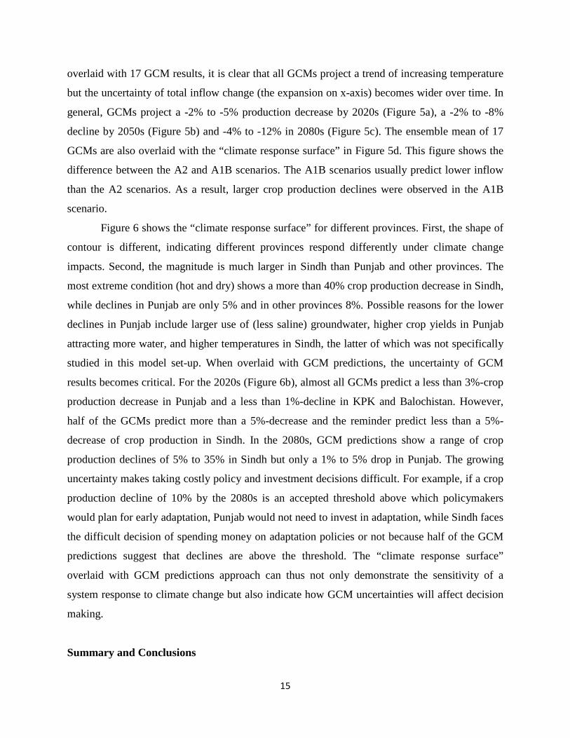
Figure 6 shows the “climate response surface” for different provinces. First, the shape of

contour is different, indicating different provinces respond differently under climate change

impacts. Second, the magnitude is much larger in Sindh than Punjab and other provinces. The

most extreme condition (hot and dry) shows a more than 40% crop production decrease in Sindh,

while declines in Punjab are only 5% and in other provinces 8%. Possible reasons for the lower

declines in Punjab include larger use of (less saline) groundwater, higher crop yields in Punjab

attracting more water, and higher temperatures in Sindh, the latter of which was not specifically

studied in this model set-up. When overlaid with GCM predictions, the uncertainty of GCM

results becomes critical. For the 2020s (Figure 6b), almost all GCMs predict a less than 3%-crop

production decrease in Punjab and a less than 1%-decline in KPK and Balochistan. However,

half of the GCMs predict more than a 5%-decrease and the reminder predict less than a 5%-

decrease of crop production in Sindh. In the 2080s, GCM predictions show a range of crop

production declines of 5% to 35% in Sindh but only a 1% to 5% drop in Punjab. The growing

uncertainty makes taking costly policy and investment decisions difficult. For example, if a crop

production decline of 10% by the 2080s is an accepted threshold above which policymakers

would plan for early adaptation, Punjab would not need to invest in adaptation, while Sindh faces

the difficult decision of spending money on adaptation policies or not because half of the GCM

predictions suggest that declines are above the threshold. The “climate response surface”

overlaid with GCM predictions approach can thus not only demonstrate the sensitivity of a

system response to climate change but also indicate how GCM uncertainties will affect decision

making.

Summary and Conclusions

16

An up-to-date Indus Basin Model Revised (IBMR-2012) is introduced in this paper. This

hydro-agro-economic model is important to analyze inter-relationships among the climate, water,

and agriculture sectors in the Indus River Basin in Pakistan. A better understanding of these

linkages will help to guide the prioritization and planning of future investments in the basin.

The overall objective of the IBMR is to maximize the consumer and producer surplus

(CPS) for the entire Indus Basin. The primary input data of the IBMR include agronomic,

economic, hydro-climatic and institutional (Water Accord) data. Hydro-climate related

parameter sensitivity analyses (a critical step in climate change impact assessment) indicate that

stream inflows are the most sensitive hydro-climatic input in the model, followed by crop water

requirements.

We show that Sindh faces both larger climate change impacts on agriculture and larger

uncertainty regarding future climate outcomes for the province. Punjab can better deal with

adverse climate change impacts due to its larger groundwater buffer, allowing it to compensate

for some of the surface water declines.

Results of the “climate response surface” for the entire basin and different provinces

show that if a threshold of acceptable crop production decrease is given (e. g. 10%), the growing

uncertainty of GCM results over time will affect adaptation decision making differentially in

Pakistan’s provinces. Particularly, Sindh will face a much larger dilemma than Punjab and other

provinces on adaptation decisions aimed at likely conditions in the 2080s.

Policymakers in Sindh should accelerate investments in water- and crop-based adaptation

strategies, such as expanding drip irrigation, which requires less (surface) water per unit of crop

produced, as well as contemplate advanced seed technologies, particularly drought and heat-

tolerant varieties of wheat given the larger adverse climate change impacts from water stress

predicted for this province.

Several improvements could be added to the study. Some studies show that

evapotranspiration can decline even when the mean temperature has risen. This is due to the

decrease of the diurnal temperature range (Peterson et al, 1995 and Braganza et al, 2004). The

linkage between temperature and crop water requirements can be improved with more detailed

agronomic studies. The current single-year version of the IBMR-2012 can be modified into a

multi-year version and groundwater simulations could be enhanced (e.g. allowing dynamic fresh

and saline area changes). This improvement should be able to reflect the impact of climate

17

change more accurately so as to evaluate the effect of the 1991 inter-provincial accord, which

plays a critical role in the current water management scheme, under current and future climate

conditions.

Acknowledgements

The study is financially support by the World Bank project: Climate Risks on Water and

Agriculture in the Indus Basin of Pakistan. Authors would like to thank Masood Ahmad at the

World Bank for his help during the IBMR update processes. The comments and suggestions

from two anonymous reviewers and guest editors are also highly appreciated.

References

Allen, R.G., Pereira, L.S., Raes, D., Smith, M. 1998. Crop Evapotranpiration: Guildlines for computing crop water requirements, FAO Irrigation and Drainage Paper No 56. Food and Agriculture Organisation, Land and Water. Rome, Italy

Ahmad, M., Brooke, A., Kutcher, G. 1990. Guide to the Indus Basin Model Revised, World Bank, Washington, D.C.

Ahmad, M and Kutcher, G. P. 1992. Irrigation Planning with Environmental Considerations - A case study of Pakistan’s Indus Basin, World Bank Technical Paper No. 166. The World Bank, Washington, D.C.

Ahmad, M., Kutcher, G., and Meeraus, A. 1986. The Agricultural Impact of the Kalabagh Dam (As simulated by the Indus Basin Model Revised). Volumes I and II. Washington, DC: World Bank.

Akhtar, M., Ahmad, N. and Booij, M. J. 2008. The impact of climate change on the water resources of Hindukush–Karakorum–Himalaya region under different glacier coverage scenarios. Journal of Hydrology, 355, 148-163.

Alam, N and Olsthoorn, T.N. 2011. Sustainable conjunctive use of surface and groundwater: modeling on the basin scale. International Journal of Natural Resources and Marine Sciences, 1: 1-12.

Archer, D. R. 2003. Contrasting hydrological regimes in the upper Indus Basin. Journal of Hydrology, 274, 198-210.

Bookhagen, B., and Burbank D. W. 2010. Toward a complete Himalayan hydrological budget: Spatiotemporal distribution of snowmelt and rainfall and their impact on river discharge, J. Geophys. Res., 115, F03019, doi:10.1029/2009JF001426.

Briscoe, J. and Qamar, U. eds. 2006. Pakistan’s Water Economy: Running Dry. Washington: World Bank, Washington, D.C.

Braganza, K., Karoly, D. J. and Arblaster J. M. 2004. Diurnal temperature range as an index of global climate change during the twentieth century, Geophys. Res. Lett., 31(13), 1-4.

18

Brown, C., Hansen, J. W. 2008. Agricultural Water Management and Climate Risk. Report to the Bill and Melinda Gates Foundation. IRI Tech. Rep. No. 08-01. International Research Institute for Climate and Society, Palisades, New York, USA. 19 pp.

Brown, C. and Wilby, R. L. 2012. An Alternate Approach to Assessing Climate Risks. Eos, 92, 401-403.

Commission on Science and Technology for Sustainable Development in the South (COMSATS). 2003. Water Resources in the South: Present Scenario and Future Prospects, COMSATS, Islamabad, Pakistan.

Duloy, J. H. and O’Mara, G. T. 1984. Issues of Efficiency and Interdependence in water resource investments: lessons from the Indus basin of Pakistan. Washington: World Bank, Washington, D.C.

Flowler, H. J. and Archer, D. R. 2006. Conflicting Signals of Climate Change in the Upper Indus Basin. Journal of Climate, 19, 4276-4293.

Immerzeel, W. W., van Beek, L. P. H. and Bierkens, M. F. P. 2010. Climate Change will Affect the Asian Water Towers, Science, 328, 1382-1385.

Islam, S., N. Rehman, M. M. Sheikh, and A. M. Khan. 2009a. Assessment of Future Changes in Temperature Related Extreme Indices over Pakistan Using Regional Climate Model PRECIS, GCISC-RR-05.” Global Change Impact Study Centre, Islamabad, Pakistan.

Islam, S., N. Rehman, M. M. Sheikh, and A. M. Khan. 2009b. “Climate Change Projections for Pakistan, Nepal and Bangladesh for SRES A2 and A1B Scenarios Using Outputs of 17 GCMs Used in IPCC-AR4, GCISC-RR-03.” Global Change Impact Study Centre, Islamabad, Pakistan.

Jeelani, G., Feddema, J. J., van der Veen, C. J. and Stearns L. 2012. Role of snow and glacier melt in controlling river hydrology in Liddar watershed (western Himalaya) under current and future climate, Water Resour. Res., 48, W12508, doi:10.1029/2011WR011590.

Kaab, A., Berthier, E., Nuth, C., Gardelle, J. and Arnaud, Y. 2012. Contrasting Patterns of Early Twenty-First-Century Glacier Mass Change in the Himalayas. Nature, 488, 495-498.

Kahlown, M.A. and Majeed, A. 2003. “Water-Resources Situation in Pakistan: Challenges and Future Strategies” in COMSATS’ Series of Publications on Science and Technology: Water Resources in the South: Present Scenario and Future Prospects, Islamabad, Pakistan. 221 pp.

Liniger, H., Weingartner, R., Grosjean, M. (Eds.), 1998. Mountains of the World: Water Towers for the 21st Century. Mountain Agenda for the Commission on Sustainable Development (CSD), BO12, Berne, 32 pp.

Ministry of Food and Agriculture (MINFA) 2010. Agricultural Statistics of Pakistan 2008-2009, Government of Pakistan, Islamabad, Pakistan.

Naheed, G., Rasul, G. 2010. Projections of Crop Water Requirement in Pakistan under Global Warming. Pakistan Journal of Meteorology. 7(13), 45-51.

Peterson, T. C., Golubev, V. S. and Groisman, P. Y. 1995. Evaporation losing its strength, Nature, 377(6551), 687-688.

19

Qureshi, A.S. 2011. Water Management in the Indus Basin in Pakistan: Challenges and Opportunities. Mt. Res. Dev. 31(3), 252–260.

Rehman, A. and Rehman, G. 1993. “Strategy for resource allocations and management across the hydrologic divides.” Volume III of Waterlogging and Salinity Management in the Sindh Province, Pakistan. Lahore: IWMI.

Rehman, G., Aslam, M., Jehangir, W. A., Rehman, A., Hussain, A., Ali, N., and Munawwar, H. Z. 1997. “Salinity management alternatives for the Rechna doab, Punjab, Pakistan.” Volume 3, Development of Procedural and Analytical Links. Report no. R-21.3. Lahore: IIMI [sic].

Tahir A. A., Chevallier, P., Arnaud, Y., Neppel, L and Ahmad, B. 2011. Modeling snowmelt-runoff under climate change scenarios in the Hunza River basin, Karakoram Range, Northern Pakistan, Journal of Hydrology, 409, 104-117.

WAPDA 1990. Water Sector Investment Planning Study (WSIPS). 5 vols. Lahore: WAPDA.

Wescoat, J. and Leichenko, R. 1992. Complex River Basin Management in a Changing Global Climate: Indus River Basin Case Study in Pakistan, A National Modelling Assessment. Collaborative Paper, no. 5. Boulder: CADSWES, Center for Advanced Decision Support for Water and Environmental Systems.

World Bank (WB) 2012. World Development Indicators. http://data.worldbank.org/data-catalog/world-development-indicators, accessed on 07/03/2013.

Yu, W. Yang, Y. C. E., Savitsky, A., Alford, D., Brown, C. Wescoat, J., Debowicz, D. and Robinson, S. 2013. The Indus Basin of Pakistan: The Impacts of Climate Risks on Water and Agriculture. Washington, DC: World Bank. doi: 10.1596/978-0-8213-9874-6. License: Creative Commons Attribution CC BY 3.0

20

Tables

Table 1. The hierarchal structure in the IBMR-2012: provinces, ACZs, number of canals and cropped land.

Table 2. Major IBMR-2012 outputs under baseline conditions

Table 3. Commodity gross profit breakdown for the baseline conditions (million PRs.)

Table 4. On-farm cost breakdown under baseline conditions (million PRs.)

21

Figures Figure 1. The Indus River and IBMR model Agro-Climatic Zones and Canal Command Areas in

Pakistan

Figure 2. The water balance in the IBMR-2012

Figure 3. The impact of changes in inflow on IBMR - 2012 outputs

Figure 4. The impact of changes in temperature (crop water requirements) on IBMR-2012

outputs

Figure 5. The basin-wide “climate response surface” of crop production changes (a) 2020s; (b)

2050s; (c) 2080s and (d) ensemble GCM mean

Figure 6. The “climate response surface” of crop production changes in Punjab, Sindh and other

provinces (a) 2020s; (b) 2050s and (c) 2080s

Figure 1. The Indus River and IBMR model Agro-Climatic Zones and Canal Command Areas in

Pakistan

Figure 2. The water balance in the IBMR-2012. Notes: The solid lines indicate the root zone water balance components which supply crop water requirement. The dotted lines represent the groundwater balance components that are tracked during the simulation runs. All water balance calculations are at the ACZ scale (dash zone) (Yu et al, 2013).

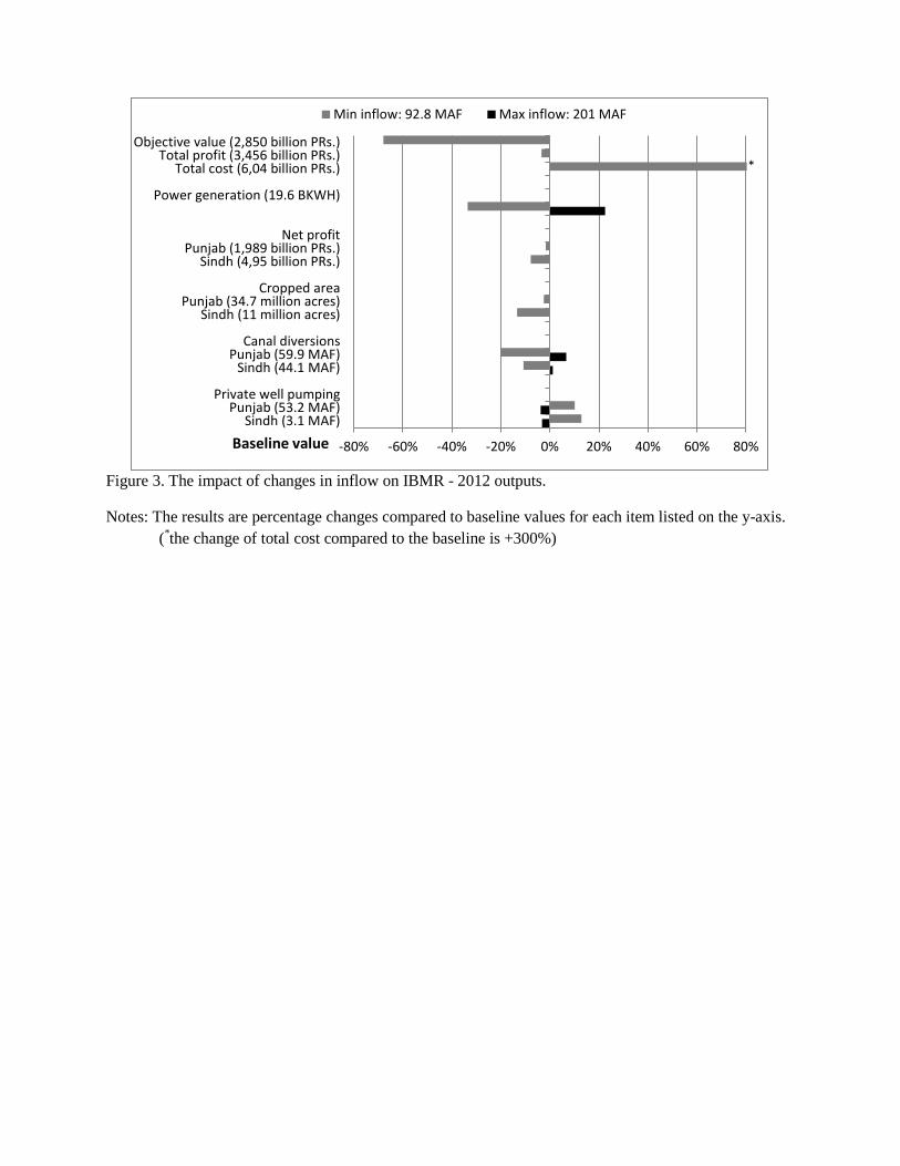
Figure 3. The impact of changes in inflow on IBMR - 2012 outputs.

Notes: The results are percentage changes compared to baseline values for each item listed on the y-axis. (*the change of total cost compared to the baseline is +300%)

-80% -60% -40% -20% 0% 20% 40% 60% 80%

Sindh (3.1 MAF)Punjab (53.2 MAF)

Private well pumping

Sindh (44.1 MAF)Punjab (59.9 MAF)

Canal diversions

Sindh (11 million acres)Punjab (34.7 million acres)

Cropped area

Sindh (4,95 billion PRs.)Punjab (1,989 billion PRs.)

Net profit

Power generation (19.6 BKWH)

Total cost (6,04 billion PRs.)Total profit (3,456 billion PRs.)

Objective value (2,850 billion PRs.)

Min inflow: 92.8 MAF Max inflow: 201 MAF

Baseline value

*

Figure 4. The impact of changes in temperature (crop water requirements) on IBMR-2012 outputs. Notes: The results are percentage changes compared to baseline values for each item listed on the y-axis.

(*the change of total cost compared to baseline is +207%)

-80% -60% -40% -20% 0% 20% 40% 60% 80%

Sindh (3.1 MAF)Punjab (53.2 MAF)

Private well pumping

Sindh (44.1 MAF)Punjab (59.9 MAF)

Canal diversions

Sindh (11 million acres)Punjab (34.7 million acres)

Cropped area

Sindh (4,95 billion PRs.)Punjab (1,989 billion PRs.)

Net profit

Power generation (19.6 BKWH)

Total cost (6,04 billion PRs.)Total profit (3,456 billion RPs.)

Objective value (2,850 billion PRs.)

Max Temp change: 6.5 degree C MinTemp change: 1 degree C

Baseline value

*

Figure 5. The basin-wide “climate response surface” of crop production changes (a) 2020s; (b) 2050s; (c) 2080s and (d) ensemble GCM mean.

Note: “o” represents A2 scenarios and “+” represents A1B scenarios.

(c) (d)

(b) (a)

Figure 6. The “climate response surface” of crop production changes in Punjab, Sindh and other

provinces (a) 2020s; (b) 2050s and (c) 2080s.

Note: “o” represents A2 scenarios and “+” represents A1B scenarios.

(a)

(b)

(c)

Table 1. The hierarchal structure in the IBMR-2012: provinces, ACZs, number of canals and cropped land.

Provinces ACZ Name Number of Canals

Available cropped land (million acres)

KPK

Khyber Pakhtunkhwa _kabul_swat (KPKS) 4 0.628

Khyber Pakhtunkhwa _mixed_wheat (KPMW) 1 0.892

Punjab

Punjab_mixed_wheat (PMW) 2 3.876

Punjab_cotton_wheat_west (PCWW) 4 3.177

Punjab_cotton_wheat_east (PCWE) 10 8.556

Punjab_sugarcane_wheat (PSW) 5 4.470

Punjab_rice_wheat (PRW) 6 2.801

Sindh

Sindh_cotton_wheat_north (SCWN) 7 3.941

Sindh_cotton_wheat_south (SCWS) 2 2.858

Sindh_rice_wheat_north (SRWN) 5 3.208

Sindh_rice_wheat_south (SRWS) 4 2.806

BLCH Baluchistan_rice_wheat (BRW) 3 1.858

Table 2 Major IBMR-2012 outputs under baseline conditions

Provinces Objective value (million PRs.)

Commodity total gross profit

(million PRs.)

On-farm costs (million PRs.)

Cropped area

(1000 acres)

Crop production (1000 tons)

Power generation (BKWH)

Pakistan 2,850,099 3,162,371 601,369 48,491 95,138 19.59 Punjab - 2,430,117 440,965 34,734 65,374 - Sindh - 628,036 132,823 11,057 24,905 - Others 104,218 27,582 2,701 4,859 -

Note: Others include KPK and BLCH

Table 3 Commodity gross profit breakdown for the baseline conditions (million PRs.) Crops Pakistan Punjab Sindh Others

Basmati rice 749,694 749,694 0 0 Irrigated rice 170,466 27,733 108,530 34,204

Cotton 674,609 552,092 122,190 327 Gram 36,101 20,860 12,810 2,431 Maize 70,457 44,542 692 25,223

Mus+rap 2,574 1,923 7 645 Sugarcane 245,950 156,249 78,764 10,937

Wheat 418,049 377,301 35,080 5,669 Potato 111,421 108,316 682 2,424 Onion 56,891 18,360 37,187 1,344 Chili 35,674 17,685 17,962 27

Cow-milk 144,051 76,608 64,160 3,282 Buffalo-milk 446,434 278,755 149,973 17,706

All 3,162,371 2,430,117 628,036 104,218

Table 4 On-farm cost breakdown under baseline conditions (million PRs.) Costs Pakistan Punjab Sindh Others

Seed 38,434 27,035 9,189 2,210 Labor 205,834 145,040 51,970 8,824 Miscellaneous 47,343 37,711 8,756 876 Protein 2,488 1,988 401 98 Fertilizer 120,082 79,972 33,261 6,849 Private well 45,930 42,942 2,530 458 Livestock 735 432 273 30 Tractor 140,524 105,844 26,442 8,238