Embed Size (px)
Citation preview
DRAFTAn Introduction to Gravity in the Solar System
Marc A. MurisonU.S. Naval Observatory, Washington, DC
25 October, 2005
Abstract
We discuss the role of gravity in the formation of the Solar System and in the motionsof the planets and other bodies.
Subject headings: celestial mechanics—gravitation—history and philosophy of astronomy—ISM:globules—methods: analytical—methods: numerical—minor planets, asteroids—planetarysystems: formation—planetary systems: protoplanetary disks—planets and satellites: for-mation—planets and satellites: general—solar system: formation—stars: formation
The XML version of this document is available on the web athttp://www.alpheratz.net/murison/papers/SolarSystemGravity/SolarSystemGravity.xml
The PDF version of this document is available on the web athttp://www.alpheratz.net/murison/papers/SolarSystemGravity/SolarSystemGravity.pdf
1
DRAFT1 Introduction 3
2 Formation of the Solar System 42.1 We Are Made of “Star Stuff” . . . . . . . . . . . . . . . . . . . . . . . . . . 42.2 A Miracle Occurs . . . . . . . . . . . . . . . . . . . . . . . . . . . . . . . . . 52.3 How do Planets Form? . . . . . . . . . . . . . . . . . . . . . . . . . . . . . . 6
3 Of Human Flailings, or History, Shmistory! 10
4 What Does Gravity Do? 154.1 Kepler the Mystic . . . . . . . . . . . . . . . . . . . . . . . . . . . . . . . . 164.2 Newton’s Notions . . . . . . . . . . . . . . . . . . . . . . . . . . . . . . . . . 18
4.2.1 The Three Laws of Motion . . . . . . . . . . . . . . . . . . . . . . . 184.2.2 The Universal Law of Gravity . . . . . . . . . . . . . . . . . . . . . . 20
4.3 Circular Motion . . . . . . . . . . . . . . . . . . . . . . . . . . . . . . . . . . 21
5 What IS Gravity? 215.1 Einstein and Geometry . . . . . . . . . . . . . . . . . . . . . . . . . . . . . . 215.2 Of Strings and Other Wiggly Things . . . . . . . . . . . . . . . . . . . . . . 23
6 Of Tintinnabulation and Children Swinging,or the Music of 1-Spheres and Resonances 246.1 What is a Resonance? . . . . . . . . . . . . . . . . . . . . . . . . . . . . . . 246.2 Mean-Motion Resonances and the Asteroids . . . . . . . . . . . . . . . . . . 25
6.2.1 Mean-Motion Resonances in the Main Belt . . . . . . . . . . . . . . 256.2.2 A Few Resonance Orbit Examples . . . . . . . . . . . . . . . . . . . 276.2.3 Resonances and Chaotic Asteroids . . . . . . . . . . . . . . . . . . . 31
6.3 Secular Resonances . . . . . . . . . . . . . . . . . . . . . . . . . . . . . . . . 346.4 Higher Order Mean Motion Resonances and the Origins of Chaos . . . . . . 34
7 Asteroid Noise 357.1 Two Kinds of Noise . . . . . . . . . . . . . . . . . . . . . . . . . . . . . . . 357.2 The Asteroid Mass Distribution . . . . . . . . . . . . . . . . . . . . . . . . . 367.3 The Noisy Motions of the Planets . . . . . . . . . . . . . . . . . . . . . . . . 41
7.3.1 Changes in the Orbital Elements . . . . . . . . . . . . . . . . . . . . 417.3.2 Power Spectra . . . . . . . . . . . . . . . . . . . . . . . . . . . . . . 447.3.3 The Destruction of Manifolds in Phase Space . . . . . . . . . . . . . 45
2
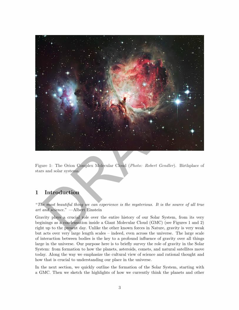
DRAFTFigure 1: The Orion Complex Molecular Cloud (Photo: Robert Gendler). Birthplace ofstars and solar systems.
1 Introduction
“The most beautiful thing we can experience is the mysterious. It is the source of all trueart and science.” —Albert Einstein
Gravity plays a crucial role over the entire history of our Solar System, from its verybeginings as a condensation inside a Giant Molecular Cloud (GMC) (see Figures 1 and 2)right up to the present day. Unlike the other known forces in Nature, gravity is very weakbut acts over very large length scales – indeed, even across the universe. The large scaleof interaction between bodies is the key to a profound influence of gravity over all thingslarge in the universe. Our purpose here is to briefly survey the role of gravity in the SolarSystem: from formation to how the planets, asteroids, comets, and natural satellites movetoday. Along the way we emphasize the cultural view of science and rational thought andhow that is crucial to understanding our place in the universe.
In the next section, we quickly outline the formation of the Solar System, starting witha GMC. Then we sketch the highlights of how we currently think the planets and other
3
DRAFTbodies formed from this tremendous accumulation of gas and dust. In Section 3 we listimportant milestones of human thought regarding the world and the universe, as well asthe gradual realization of the order of things and, at last, of how planetary motion behaves.We realize that observation must always take precedence over ideology and preconceivednotions if the goal is to learn about the world. In Section 4 we review the basic classicalnotions of how gravity works – that is, the nuts and bolts one needs to describe and predictplanetary motions. In Section 5 we make a brief attempt to say what gravity is, as opposedto what it does. We conclude in Section 6 with a select smorgasbord of current researchtopics concerning gravity and its effects in the Solar System (all of which are fascinatingand very exciting, of course!).
2 Formation of the Solar System
2.1 We Are Made of “Star Stuff”
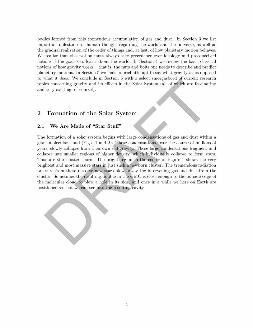
The formation of a solar system begins with large condensations of gas and dust within agiant molecular cloud (Figs. 1 and 2). These condensations, over the course of millions ofyears, slowly collapse from their own self-gravity. These large condensations fragment andcollapse into smaller regions of higher density, which individually collapse to form stars.Thus are star clusters born. The bright region in the center of Figure 1 shows the verybrightest and most massive stars in just such a newborn cluster. The tremendous radiationpressure from these massive new stars blows away the intervening gas and dust from thecluster. Sometimes the resulting bubble in the GMC is close enough to the outside edge ofthe molecular cloud to blow a hole in its side, and once in a while we here on Earth arepositioned so that we can see into the resulting cavity.
4
DRAFTFigure 2: Barnard 68, an isolated dark globule ( Photo: European Southern Observatory).Stars and their solar systems form when condensations inside globules of gas and dust suchas this one collapse due to their own gravity.
2.2 A Miracle Occurs
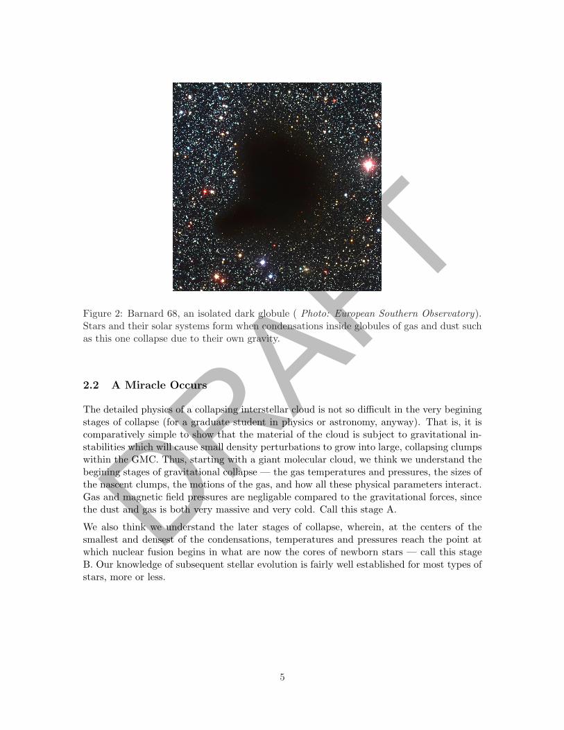
The detailed physics of a collapsing interstellar cloud is not so difficult in the very beginingstages of collapse (for a graduate student in physics or astronomy, anyway). That is, it iscomparatively simple to show that the material of the cloud is subject to gravitational in-stabilities which will cause small density perturbations to grow into large, collapsing clumpswithin the GMC. Thus, starting with a giant molecular cloud, we think we understand thebegining stages of gravitational collapse — the gas temperatures and pressures, the sizes ofthe nascent clumps, the motions of the gas, and how all these physical parameters interact.Gas and magnetic field pressures are negligable compared to the gravitational forces, sincethe dust and gas is both very massive and very cold. Call this stage A.
We also think we understand the later stages of collapse, wherein, at the centers of thesmallest and densest of the condensations, temperatures and pressures reach the point atwhich nuclear fusion begins in what are now the cores of newborn stars — call this stageB. Our knowledge of subsequent stellar evolution is fairly well established for most types ofstars, more or less.
5
DRAFTHowever, it is not yet understood how the transition from stage A to stage B works indetail. We know it must happen, since we observe (via radio and infrared astronomy) giantmolecular clouds containing interior clumps in the process of collapsing, and we observenewly-ignited young stars (called young stellar objects, also studied at radio and infraredwavelengths) embedded in more-evolved GMCs. In that in-between stage, gas pressure andmagnetic field pressure — both of which act to counter the gravitational forces — are nolonger ignorable and must be taken into account, yet the physical conditions inside theseclouds is not well-enough known to allow us to do so.
Once we get past this stage of star formation and ignition, we then have the issue of formingplanets out of the leftover material.
2.3 How do Planets Form?
We don’t really know.
However, we do have some good ideas based on the
1. known physical processes,
2. educated guesses about the physical conditions that must have been present duringthe planet formation stage of the Solar System, and
3. sophisticated computer modeling
6

DRAFTcurrently at our disposal. Planet formation is currently a very active area of research, anda more or less consistent picture is forming. The leftover material from formation of thecentral star is orbiting around the star, so it forms a flattened disk, called a protoplanetarydisk (Figure 3). Starting with a disk of material circling a young central star, one candistinguish two, or perhaps three, regimes of subsequent planet formation: inner rockyplanets, outer gas giants, and outer rocky/icy worlds.
Figure 3: The inner part of the protoplanetary disk surrounding the star AB Aurigae.The dark cross is the shadow of an occulting bar that blocks most of the light from thecentral star. The diagonal lines are artifacts leftover from the removal of the diffractionspikes caused by the Hubble Space Telescope’s secondary mirror supports. ( Photo: SpaceTelescope Science Institute)
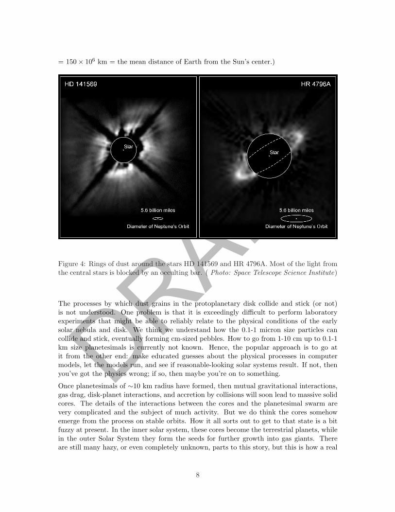
The inner solar system planets (“terrestrial planets”) are thought to have formed by solidbody accretion of kilometer-sized objects, which in turn were formed via collisional growthstarting with micron-sized dust grains from a late-stage protoplanetary disk. Dust grainsare present throughout the solar nebula as it collapses from the GMC. After the disk ofmaterial orbiting around the new Sun is formed, the dust grains, being heavier than the gasparticles, sink towards the disk midplane and become concentrated (and therefore muchmore likely to suffer collisions with other dust grains). Figure 4 shows images of dustrings around two newly-formed stars. The timescale for settling to the disk midplane andgrowing to cm size particles is roughly 104-105 years at 1 AU. (1 AU = 1 Astronomical Unit
7
DRAFT= 150× 106 km = the mean distance of Earth from the Sun’s center.)
Figure 4: Rings of dust around the stars HD 141569 and HR 4796A. Most of the light fromthe central stars is blocked by an occulting bar. ( Photo: Space Telescope Science Institute)
The processes by which dust grains in the protoplanetary disk collide and stick (or not)is not understood. One problem is that it is exceedingly difficult to perform laboratoryexperiments that might be able to reliably relate to the physical conditions of the earlysolar nebula and disk. We think we understand how the 0.1-1 micron size particles cancollide and stick, eventually forming cm-sized pebbles. How to go from 1-10 cm up to 0.1-1km size planetesimals is currently not known. Hence, the popular approach is to go atit from the other end: make educated guesses about the physical processes in computermodels, let the models run, and see if reasonable-looking solar systems result. If not, thenyou’ve got the physics wrong; if so, then maybe you’re on to something.
Once planetesimals of ∼10 km radius have formed, then mutual gravitational interactions,gas drag, disk-planet interactions, and accretion by collisions will soon lead to massive solidcores. The details of the interactions between the cores and the planetesimal swarm arevery complicated and the subject of much activity. But we do think the cores somehowemerge from the process on stable orbits. How it all sorts out to get to that state is a bitfuzzy at present. In the inner solar system, these cores become the terrestrial planets, whilein the outer Solar System they form the seeds for further growth into gas giants. Thereare still many hazy, or even completely unknown, parts to this story, but this is how a real
8
DRAFTsolar system might get to the point of having a retinue of Earth-mass objects orbiting thenascent central star.
For the gas giants, there appear to be two possible formation scenarios. First, the planetscould have formed via fragmentation of the protoplanetary disk and subsequent collapseof the fragments into planets. This cannot work for the inner solar system due to thehigher temperatures and the higher radiation and particle wind from the Sun, preventinglarge blobs of material from collapsing before they’re eaten away and dispersed. The diskfragmentation occurs because rotating disks of material are subject to various gravitationaland fluid instabilities. The advantage of this model is that, once fragmentation begins,planets can form very quickly, which would be consistent with observations of extrasolarplanetary systems. However, it is difficult to get a protoplanetary disk to fragment in sucha way that planets could actually form. Condensation of fragments into planets requiresaxisymmetric disk fragmentation modes. Yet protoplanetary disks are relatively immuneto axisymmetric instabilities and prefer asymmetric modes such as spiral waves, for whichsubsequent condensation is difficult.
The second outer planet formation scenario is accretion of gas and dust onto planetarycores. Again, the details are complicated and the subject of much research at present. Oneof the major problems is one of timing: at a certain point the cores become massive enoughthat runaway growth occurs. It is difficult to form planets quickly enough in this scenario,as the slow buildup before the runaway growth phase can last a very long time, posing aproblem with modern observations. Thus, both modes of outer planet formation have theirfeatures and problems, and it is not clear which actually occurs or how in detail.
9
DRAFT3 Of Human Flailings, or History, Shmistory!
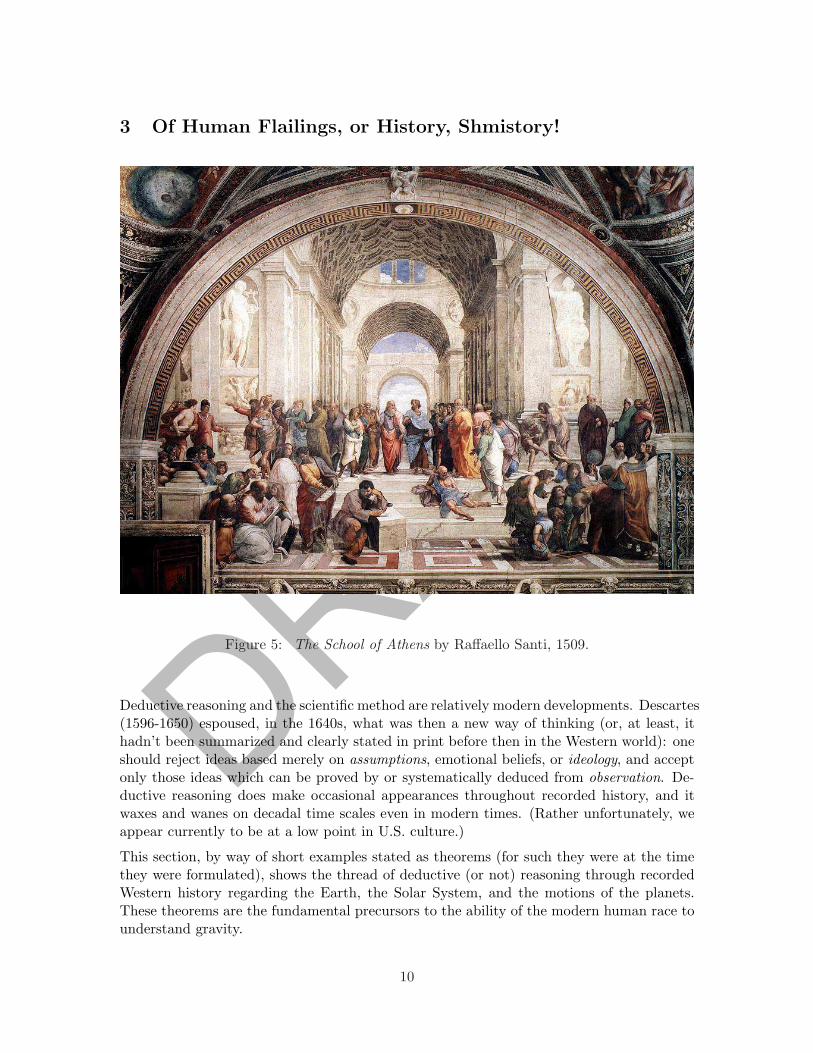
Figure 5: The School of Athens by Raffaello Santi, 1509.
Deductive reasoning and the scientific method are relatively modern developments. Descartes(1596-1650) espoused, in the 1640s, what was then a new way of thinking (or, at least, ithadn’t been summarized and clearly stated in print before then in the Western world): oneshould reject ideas based merely on assumptions, emotional beliefs, or ideology, and acceptonly those ideas which can be proved by or systematically deduced from observation. De-ductive reasoning does make occasional appearances throughout recorded history, and itwaxes and wanes on decadal time scales even in modern times. (Rather unfortunately, weappear currently to be at a low point in U.S. culture.)
This section, by way of short examples stated as theorems (for such they were at the timethey were formulated), shows the thread of deductive (or not) reasoning through recordedWestern history regarding the Earth, the Solar System, and the motions of the planets.These theorems are the fundamental precursors to the ability of the modern human race tounderstand gravity.
10
DRAFTTheorem 1. (Early Mesopotamia) The Earth is flat.
Theorem 2. (Ancient Greeks and others) Things go up. They come back down.
Remark. These two theorems seem entirely self-evident. The first, of course, is quite wrong.It would not be until Isaac Newton before the mechanics of the second was understood, andthat it, too, is only conditionally right. (Hint: rocket ship.)
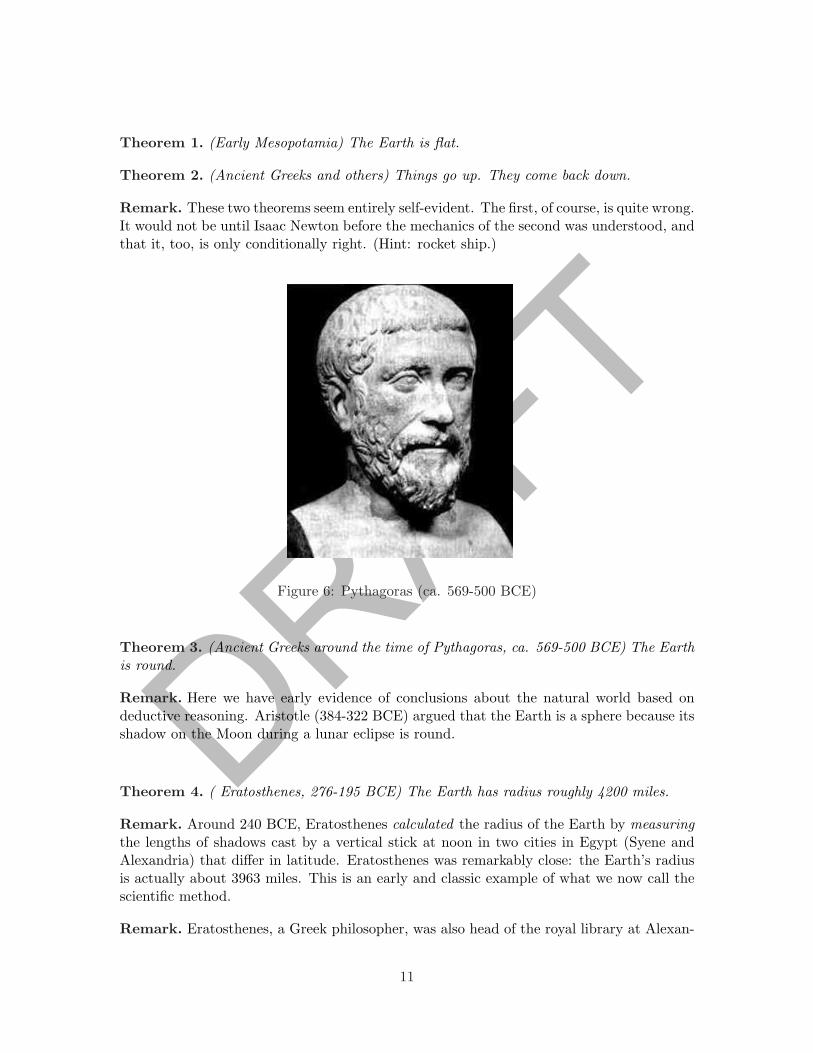
Figure 6: Pythagoras (ca. 569-500 BCE)
Theorem 3. (Ancient Greeks around the time of Pythagoras, ca. 569-500 BCE) The Earthis round.
Remark. Here we have early evidence of conclusions about the natural world based ondeductive reasoning. Aristotle (384-322 BCE) argued that the Earth is a sphere because itsshadow on the Moon during a lunar eclipse is round.
Theorem 4. ( Eratosthenes, 276-195 BCE) The Earth has radius roughly 4200 miles.
Remark. Around 240 BCE, Eratosthenes calculated the radius of the Earth by measuringthe lengths of shadows cast by a vertical stick at noon in two cities in Egypt (Syene andAlexandria) that differ in latitude. Eratosthenes was remarkably close: the Earth’s radiusis actually about 3963 miles. This is an early and classic example of what we now call thescientific method.
Remark. Eratosthenes, a Greek philosopher, was also head of the royal library at Alexan-
11
DRAFTdria, the greatest library of classical antiquity. Chalk one up for librarians.
Theorem 5. ( Aristotle, 384-322 BCE) The Earth is at the center of the Universe.
Corollary 1. The heavens, including the Sun and planets, revolve around the Earth.
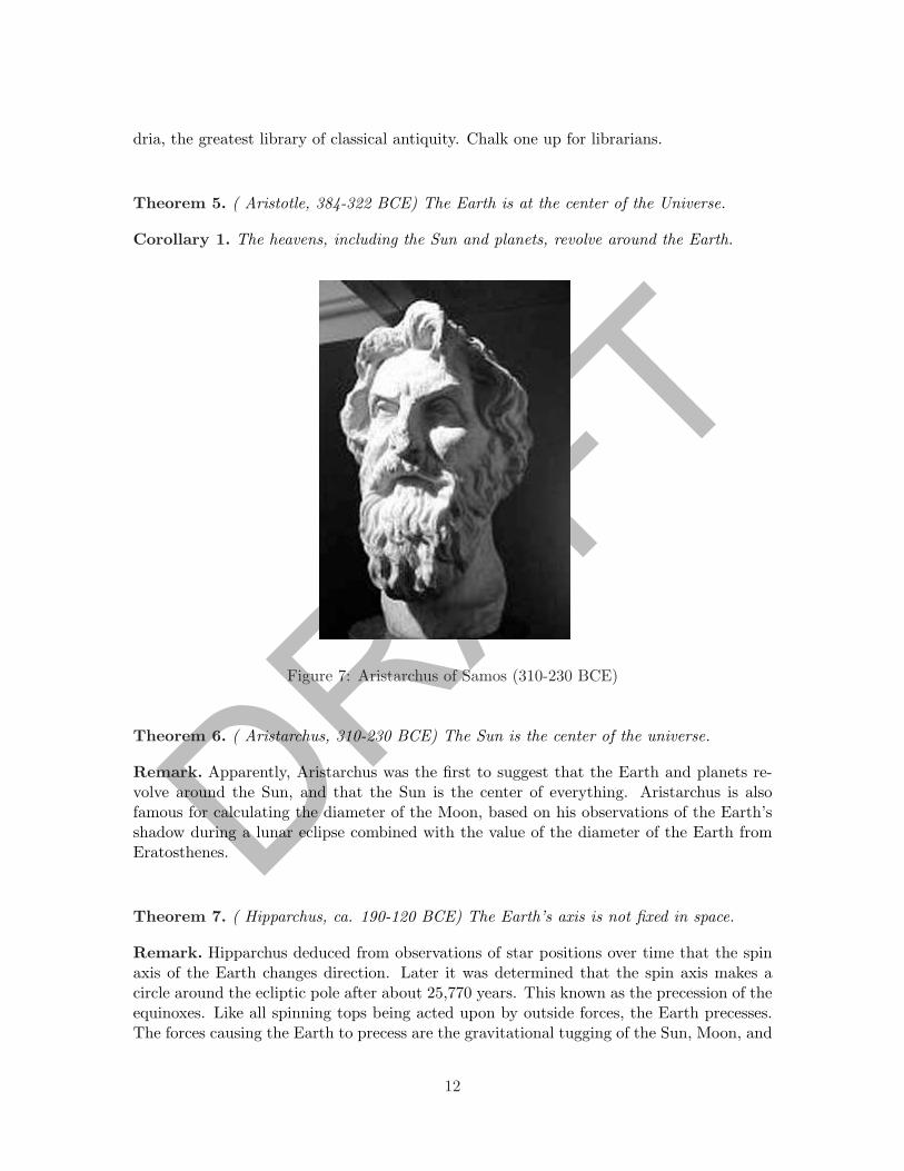
Figure 7: Aristarchus of Samos (310-230 BCE)
Theorem 6. ( Aristarchus, 310-230 BCE) The Sun is the center of the universe.
Remark. Apparently, Aristarchus was the first to suggest that the Earth and planets re-volve around the Sun, and that the Sun is the center of everything. Aristarchus is alsofamous for calculating the diameter of the Moon, based on his observations of the Earth’sshadow during a lunar eclipse combined with the value of the diameter of the Earth fromEratosthenes.
Theorem 7. ( Hipparchus, ca. 190-120 BCE) The Earth’s axis is not fixed in space.
Remark. Hipparchus deduced from observations of star positions over time that the spinaxis of the Earth changes direction. Later it was determined that the spin axis makes acircle around the ecliptic pole after about 25,770 years. This known as the precession of theequinoxes. Like all spinning tops being acted upon by outside forces, the Earth precesses.The forces causing the Earth to precess are the gravitational tugging of the Sun, Moon, and
12
DRAFTplanets on the equatorial bulge of the Earth.
Theorem 8. ( Ptolemy, ca. 2nd century CE) The planets move on epicycles in theirmotions around the Earth.
Remark. Here we have a classic example of muddled thinking. Belief had it that the Earthwas the center of everything. Observations of the motions of the planets on the sky conflictedwith this model. So Ptolemy tried to patch the model up by adding epicycles, rather thanrethinking his assumptions and model. “Adding epicycles” is now a common metaphor forthis kind of mistaken thinking. This is not to say that avoiding this pitfall is easy. Oftenwe are faced with an inadequate model which mostly works but which we suspect may befundamentally flawed, yet there is at the time no other recourse than to continue use ofthe flawed model while searching for a better one. However, using a flawed model with fullknowledge that something is wrong is quite different from stubbornly sticking with mistakenassumptions in the face of contradictory observational evidence.
Theorem 9. (Early Christian authors, ∼200-550 CE) The Earth is flat.
Remark. Rational thought and observed fact can be lost, forgotten, or buried by ideologyand ignorance.
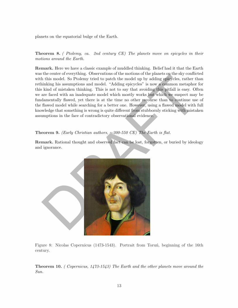
Figure 8: Nicolas Copernicus (1473-1543). Portrait from Torun, beginning of the 16thcentury.
Theorem 10. ( Copernicus, 1473-1543) The Earth and the other planets move around theSun.
13
DRAFTRemark. The scientific revolution of Western Europe begins.
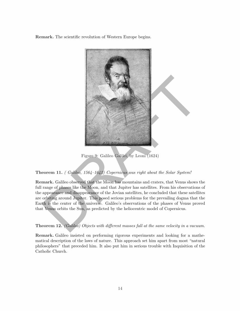
Figure 9: Galileo Galilei, by Leoni (1624)
Theorem 11. ( Galileo, 1564–1642) Copernicus was right about the Solar System!
Remark. Galileo observed that the Moon has mountains and craters, that Venus shows thefull range of phases like the Moon, and that Jupiter has satellites. From his observations ofthe appearance and disappearance of the Jovian satellites, he concluded that these satellitesare orbiting around Jupiter. This posed serious problems for the prevailing dogma that theEarth is the center of the universe. Galileo’s observations of the phases of Venus provedthat Venus orbits the Sun, as predicted by the heliocentric model of Copernicus.
Theorem 12. (Galileo) Objects with different masses fall at the same velocity in a vacuum.
Remark. Galileo insisted on performing rigorous experiments and looking for a mathe-matical description of the laws of nature. This approach set him apart from most “naturalphilosophers” that preceded him. It also put him in serious trouble with Inquisition of theCatholic Church.
14
DRAFT4 What Does Gravity Do?
“Nevertheless, it does move.” —Galileo Galilei, 1633
By now we realize that this mysterious force we call gravity fundamentally affects thestructure of and movements within the Solar System. With the advent of the Age ofEnlightenment and the subsequent explosion of mathematics and curiosity about the naturalworld, we naturally turn to gravity and wonder how it works and what it is. The latterturns out to be an exceedingly deep question. If we can’t quite discern its nature, thensurely we can apply mathematics and observation in order to characterize what it does andhow it makes moving objects behave. Employing mathematics and physical reasoning incombination, one can actually characterize the effects of this thing called gravity and evenpredict effects not yet observed. This new way of thinking reached its pinnacle with IsaacNewton and his laws of motion and gravity.
Newton’s mathematical explorations and physical explanations are founded on the work ofKepler before him. (Indeed, it was Newton who famously said, in a letter to Robert Hookein 1676, “If I have seen further it is by standing on the shoulders of Giants.” This wasprobably meant as an insult, as Newton and Hooke disliked each other greatly, and Hookewas of very short stature. The origins of the quote are attributed to the young Romanpoet Lucan (39-65 CE), in his epic poem The Civil War, “Pigmies placed on the shouldersof giants see more than the giants themselves.” However, the ten surviving books of the(probably unfinished) Civil War do not contain the quote.) We leave aside for now thequestion of the nature of gravity and consider for a bit what it does – that is, how we canquantitatively characterise the basic effects of gravity.
15
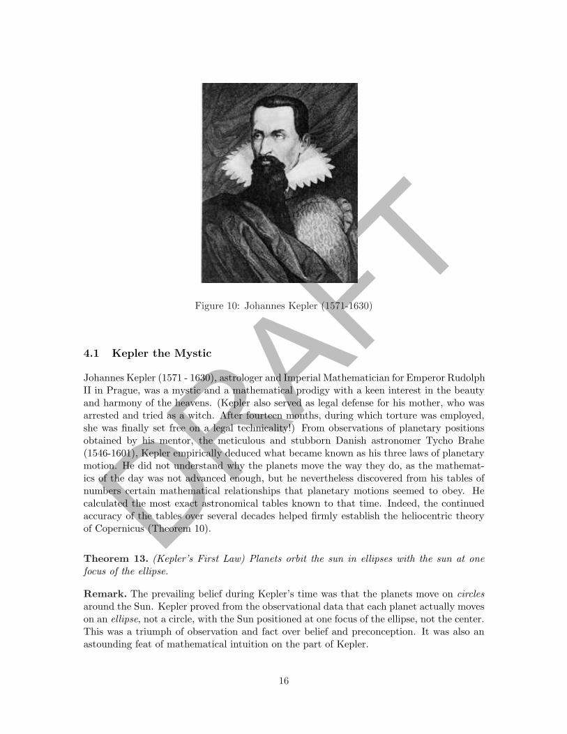
DRAFTFigure 10: Johannes Kepler (1571-1630)
4.1 Kepler the Mystic
Johannes Kepler (1571 - 1630), astrologer and Imperial Mathematician for Emperor RudolphII in Prague, was a mystic and a mathematical prodigy with a keen interest in the beautyand harmony of the heavens. (Kepler also served as legal defense for his mother, who wasarrested and tried as a witch. After fourteen months, during which torture was employed,she was finally set free on a legal technicality!) From observations of planetary positionsobtained by his mentor, the meticulous and stubborn Danish astronomer Tycho Brahe(1546-1601), Kepler empirically deduced what became known as his three laws of planetarymotion. He did not understand why the planets move the way they do, as the mathemat-ics of the day was not advanced enough, but he nevertheless discovered from his tables ofnumbers certain mathematical relationships that planetary motions seemed to obey. Hecalculated the most exact astronomical tables known to that time. Indeed, the continuedaccuracy of the tables over several decades helped firmly establish the heliocentric theoryof Copernicus (Theorem 10).
Theorem 13. (Kepler’s First Law) Planets orbit the sun in ellipses with the sun at onefocus of the ellipse.
Remark. The prevailing belief during Kepler’s time was that the planets move on circlesaround the Sun. Kepler proved from the observational data that each planet actually moveson an ellipse, not a circle, with the Sun positioned at one focus of the ellipse, not the center.This was a triumph of observation and fact over belief and preconception. It was also anastounding feat of mathematical intuition on the part of Kepler.
16
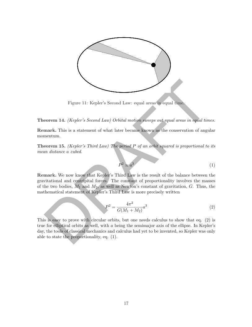
DRAFTFigure 11: Kepler’s Second Law: equal areas in equal time.
Theorem 14. (Kepler’s Second Law) Orbital motion sweeps out equal areas in equal times.
Remark. This is a statement of what later became known as the conservation of angularmomentum.
Theorem 15. (Kepler’s Third Law) The period P of an orbit squared is proportional to itsmean distance a cubed.
P 2 ∝ a3 (1)
Remark. We now know that Kepler’s Third Law is the result of the balance between thegravitational and centripital forces. The constant of proportionality involves the massesof the two bodies, M1 and M2, as well as Newton’s constant of gravitation, G. Thus, themathematical statement of Kepler’s Third Law is more precisely written
P 2 =4π2
G(M1 + M2)a3 (2)
This is easy to prove with circular orbits, but one needs calculus to show that eq. (2) istrue for elliptical orbits as well, with a being the semimajor axis of the ellipse. In Kepler’sday, the tools of classical mechanics and calculus had yet to be invented, so Kepler was onlyable to state the proportionality, eq. (1).
17
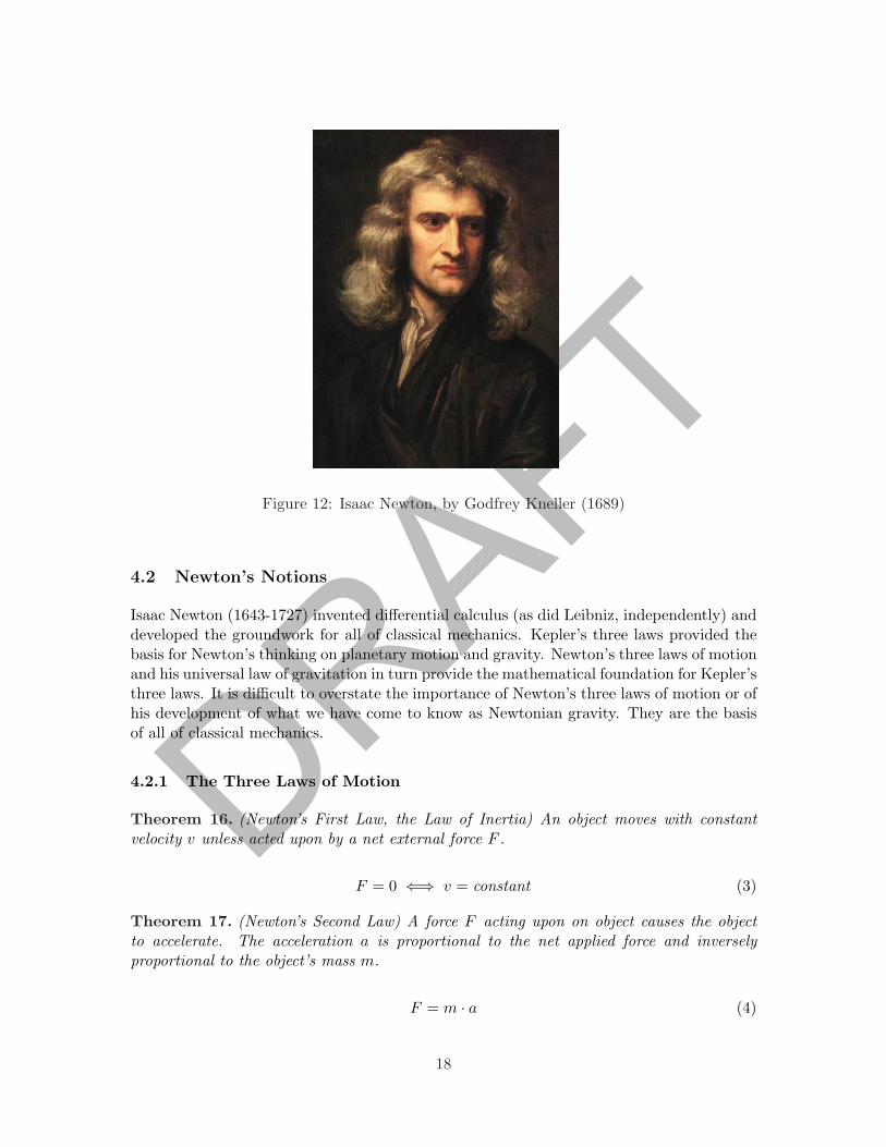
DRAFTFigure 12: Isaac Newton, by Godfrey Kneller (1689)
4.2 Newton’s Notions
Isaac Newton (1643-1727) invented differential calculus (as did Leibniz, independently) anddeveloped the groundwork for all of classical mechanics. Kepler’s three laws provided thebasis for Newton’s thinking on planetary motion and gravity. Newton’s three laws of motionand his universal law of gravitation in turn provide the mathematical foundation for Kepler’sthree laws. It is difficult to overstate the importance of Newton’s three laws of motion or ofhis development of what we have come to know as Newtonian gravity. They are the basisof all of classical mechanics.
4.2.1 The Three Laws of Motion
Theorem 16. (Newton’s First Law, the Law of Inertia) An object moves with constantvelocity v unless acted upon by a net external force F .
F = 0 ⇐⇒ v = constant (3)
Theorem 17. (Newton’s Second Law) A force F acting upon on object causes the objectto accelerate. The acceleration a is proportional to the net applied force and inverselyproportional to the object’s mass m.
F = m · a (4)
18
DRAFTRemark. Since velocity is the change in distance with time, v = dx
dt , and since accelerationis the change in velocity with time, a = dv
dt , we have from eq. (4) the (vector) equationsdescribing the motion of an object due to an applied force:
dvdt = 1
m · F (v, x, t)dxdt = v
(5)
The force may be a function of time, position, or velocity.
Remark. F = ma is almost all of classical mechanics in a deceptively compact nutshell!
Theorem 18. (Newton’s Third Law) For every action there is an equal and opposite reac-tion.
Remark. Suppose body A exerts a force on body B. We will denote this force by FAB .Then
FAB = −FBA (6)
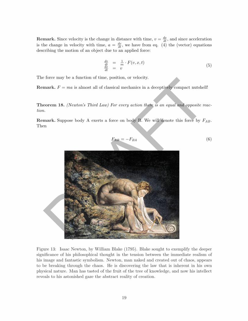
Figure 13: Isaac Newton, by William Blake (1795). Blake sought to exemplify the deepersignificance of his philosophical thought in the tension between the immediate realism ofhis image and fantastic symbolism. Newton, man naked and created out of chaos, appearsto be breaking through the chaos. He is discovering the law that is inherent in his ownphysical nature. Man has tasted of the fruit of the tree of knowledge, and now his intellectreveals to his astonished gaze the abstract reality of creation.
19
DRAFT4.2.2 The Universal Law of Gravity
“Gravity: it’s not just a good idea, it’s the law.” —bumper sticker popular with nerds
Theorem 19. (Newtonian Gravitation) Two masses M1 and M2 attract each other with aforce that is proportional to their masses and inversely proportional to the distance r betweenthem squared:
F = GM1M 2
r2(7)
Remark. This law is deceptively simple in appearance. Yet it adequately covers almost(but not quite!) all that we know and observe regarding the motions of bodies in the SolarSystem. One begins to appreciate the complexity hidden in eq. (7) by considering theequations of motion that result for a body being influenced by the Newtonian gravity ofN − 1 other perfectly spherical bodies (the so-called N-body problem):
d2−→rdt2 = −G
N−1∑
k=1
Mk∣∣−→r −−→r k
∣∣3(−→r −−→r k
)(8)
There is a similar equation for each of the other bodies. The presence of each body is feltby all of the others. Furthermore, this is a system of nonlinear equations. These propertiesrender them extremely difficult to solve, even for simplified ideal situations. However, it isjust these properties that give rise to the most interesting phenomena in dynamical systems,such as chaotic motion.
The two-body problem can be solved analytically, meaning we can write down the completedescription of the motions of the bodies using simple (or, more accurately, closed-form)mathematical functions. For example, the solution for the distance between the bodies inthe two-body problem is given by the equation for an ellipse:
r =a(1− e2
)
1 + ecosθ(9)
where e is the eccentricity and θ is the azimuthal angle. This is what Kepler discerned fromhis tables of position observations as the basic motion of a planet around the Sun. But addjust one more body and the problem cannot be solved analytically, except for certain highly-contrived circumstances. This wasn’t proved until the brilliant French mathematician andtheoretical astronomer Henri Poincare (1854-1912) came along and did it near the end of the19th century. Astronomers and mathematicians have spent over three centuries working outthe motions of the Solar System bodies using Newtonian gravity, and we are still nowhereclose to a complete description.
20
DRAFT4.3 Circular Motion
[...]Definition 1. Centripetal acceleration is the acceleration towards the center of a circularpath that keeps an object in constant circular motion. Its magnitude is
acentripetal =v2c
r(10)
where vc is the magnitude of the velocity along the circular path.
[...]
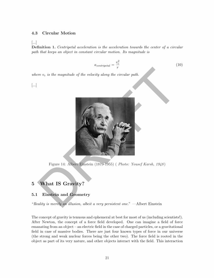
Figure 14: Albert Einstein (1879-1955) ( Photo: Yousef Karsh, 1948 )
5 What IS Gravity?
5.1 Einstein and Geometry
“Reality is merely an illusion, albeit a very persistent one.” —Albert Einstein
The concept of gravity is tenuous and ephemeral at best for most of us (including scientists!).After Newton, the concept of a force field developed. One can imagine a field of forceemanating from an object – an electric field in the case of charged particles, or a gravitationalfield in case of massive bodies. There are just four known types of force in our universe(the strong and weak nuclear forces being the other two). The force field is rooted in theobject as part of its very nature, and other objects interact with the field. This interaction
21
DRAFTproduces accelerations, and we call the effect a force. If this sounds like a highly-theoreticalconstruct, it is.
One of the serious problems with the concept of a force field in Newtonian gravity is that itrequires action at a distance, a term meaning the instantaneous propagation of force. Forexample, the Newtonian equations of gravity make no allowance for the propagation of adisturbance (say, the movement of one planet affecting another some distance away) at afinite speed, which surely must be unphysical, since everything we see, touch, and measureinvolves finite speeds. (The speed of light is very large, but even it, too, is finite.) Forexample, the disturbances in an electromagnetic field propagate at the speed of light. Wemake practical use of them as radio waves. We are able in most cases to put up with thisdisturbing flaw in Newtonian gravity, since the propagation speed of gravitational distur-bances, though finite, is still very large, so that in most applications it can be approximatedas infinite. The resulting errors are extremely small.
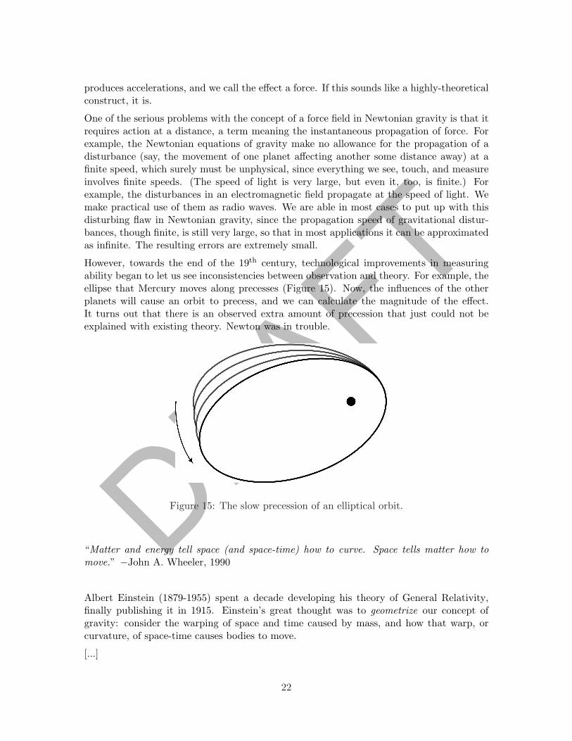
However, towards the end of the 19th century, technological improvements in measuringability began to let us see inconsistencies between observation and theory. For example, theellipse that Mercury moves along precesses (Figure 15). Now, the influences of the otherplanets will cause an orbit to precess, and we can calculate the magnitude of the effect.It turns out that there is an observed extra amount of precession that just could not beexplained with existing theory. Newton was in trouble.
Figure 15: The slow precession of an elliptical orbit.
“Matter and energy tell space (and space-time) how to curve. Space tells matter how tomove.” −John A. Wheeler, 1990
Albert Einstein (1879-1955) spent a decade developing his theory of General Relativity,finally publishing it in 1915. Einstein’s great thought was to geometrize our concept ofgravity: consider the warping of space and time caused by mass, and how that warp, orcurvature, of space-time causes bodies to move.
[...]
22
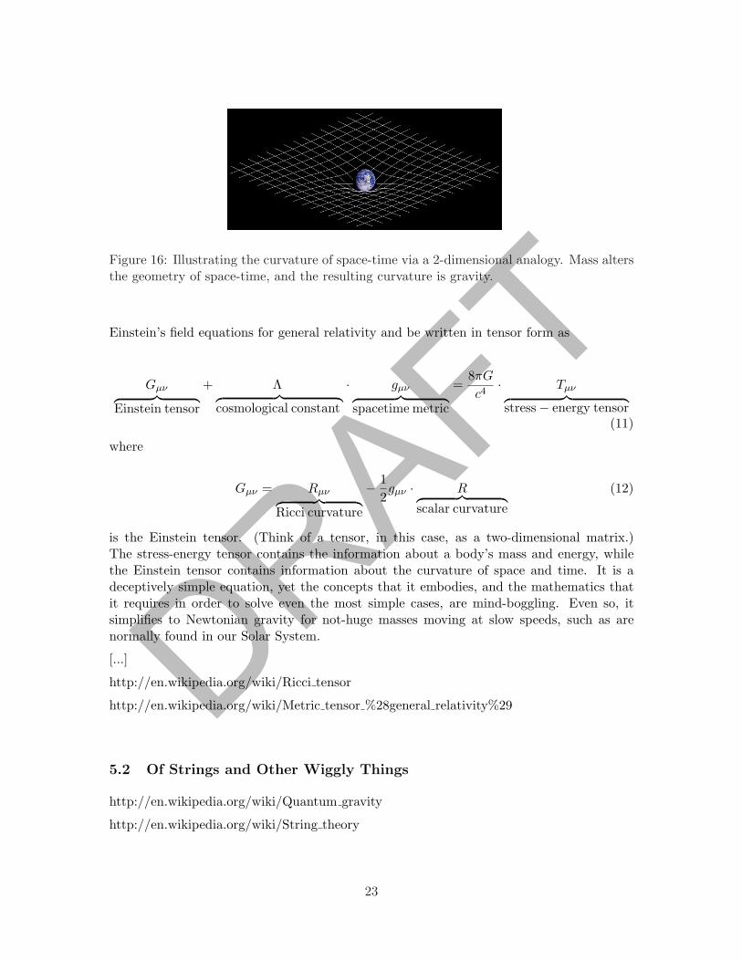
DRAFTFigure 16: Illustrating the curvature of space-time via a 2-dimensional analogy. Mass altersthe geometry of space-time, and the resulting curvature is gravity.
Einstein’s field equations for general relativity and be written in tensor form as
Gµν︷ ︸︸ ︷Einstein tensor
+ Λ︷ ︸︸ ︷cosmological constant
· gµν︷ ︸︸ ︷spacetime metric
=8πG
c4· Tµν︷ ︸︸ ︷stress− energy tensor
(11)
where
Gµν = Rµν︷ ︸︸ ︷Ricci curvature
− 12gµν · R︷ ︸︸ ︷
scalar curvature
(12)
is the Einstein tensor. (Think of a tensor, in this case, as a two-dimensional matrix.)The stress-energy tensor contains the information about a body’s mass and energy, whilethe Einstein tensor contains information about the curvature of space and time. It is adeceptively simple equation, yet the concepts that it embodies, and the mathematics thatit requires in order to solve even the most simple cases, are mind-boggling. Even so, itsimplifies to Newtonian gravity for not-huge masses moving at slow speeds, such as arenormally found in our Solar System.
[...]
http://en.wikipedia.org/wiki/Ricci tensor
http://en.wikipedia.org/wiki/Metric tensor %28general relativity%29
5.2 Of Strings and Other Wiggly Things
http://en.wikipedia.org/wiki/Quantum gravity
http://en.wikipedia.org/wiki/String theory
23
DRAFT6 Of Tintinnabulation and Children Swinging,
or the Music of 1-Spheres and Resonances
“What a tale of terror, now, their turbulency tells!” —Edgar Allan Poe, 1849
In this section, we introduce some modern work being done in Solar System dynamics. Theconcept of resonance is a recurring and underlying theme, so first we will discuss what wemean by that in the context of Solar System motions. Then we consider the simplest typeof resonance, called a mean-motion resonance, between two objects as they orbit aboutthe Sun. Secular and spin-orbit resonances are two further categories of resonance, thefirst between two planets again, and the second a special type involving the spin of anobject interacting with its own orbit. We discuss those next. Finally, we consider the nexthierarchy of mean-motion resonances: resonances inside resonances. This is a sure-fire wayof creating chaotic motions among the bodies involved.
[Okay, so what is a 1-sphere? It’s mathspeak for circle (more properly a closed curve thatcan be smoothly deformed into a circle), which is a 1-dimensional sphere. A 0-sphere isa point, a 2-sphere is what we usually think of as a “sphere”, a 3-sphere is a sphere infour-dimensional space, and so on.]
6.1 What is a Resonance?
Simply put, a resonance between any two coupled oscillatory phenomena occurs when theperiods of oscillation are an integer ratio. (It is equivalent to require that their frequenciesof oscillation are an integer ratio.) The basic idea of a resonance is familiar to anyone who
24
DRAFThas pushed a child on a swing. The swing, if pushed and then left alone, has a certainperiod of oscillation, or back-and-forth motion. Let’s call this period P . If you give theswing a small push at intervals equal or close to P , then you will be pumping energy intothe swing’s motion. It is quite surprising how the accumulation of very small pushes willsoon result in a very large amplitude of swinging. This phenomenon is resonance, and it isthe same concept no matter how complex the physics and mathematics.
Another example is that of a singer breaking a crystal wine glass. (Yes, it can be done.)The wine glass has a natural frequency of oscillation, which we call the resonant frequency.If the singer can sing a note at that resonant frequency, the sound waves transfer smallamounts of energy to the motion of the glass vibrations. In the same way you can get achild going very high on a swing with a succession of small pushes, the wine glass vibrationsbecome very large after a succession of small pushes from the sound waves from the singer’svoice. After a short time, the glass cannot handle the stresses of vibration and it shatters.
6.2 Mean-Motion Resonances and the Asteroids
In planetary motion, a mean-motion resonance is when the orbital periods of two orbitsare a ratio of integers. For example, Pluto is in a 2:3 resonance with Neptune, completingtwo orbits of the Sun in the time it takes Neptune to orbit three times. Thus, at periodicintervals, Neptune and Pluto tug each other very slightly at the same locations in space. Itturns out that resonances are of fundamental importance because of this periodic tugging.Resonances can cause either stability or instability of the associated dynamics, dependingon the stability of the associated periodic orbit.
At a stable resonance, small perturbations will not change the dynamics. The Pluto-Neptune resonance is an example. The 2:3 resonance ensures that, whenever Pluto isclosest to the Sun, Neptune is far away from Pluto, thus guaranteeing they will never havea close encounter. Another example is the case of the orbits of Jupiter’s moons Ganymede,Europa, and Io: they are in a 1:2:4 orbital resonance. The critical angle involving theirorbital longitudes, σ = LIo − 3LEuropa + 2LGanymede, librates around σ = π. (The criticalangle will be explained below, in section 6.2.2.) Hence their mean motions are such thatnIo − 3nEuropa + 2nGanymede = 0.
At an unstable resonance, small perturbations will grow, and the bodies will over timebe driven away from their resonant configuration. This can lead to some pretty strangebehavior. For example, certain resonances associated with the precession of Saturn’s orbitcause asteroids located at certain points in the asteroid belt to be driven towards the innersolar system. This is where the supply of near-earth asteroids originates.
6.2.1 Mean-Motion Resonances in the Main Belt
The effects of mean-motion resonances with Jupiter can be seen in the distribution of theasteroids. [...]
• clearing and gathering due to resonances (asteroid belt)
25
DRAFT• three-body problem and rotating reference frame
• some orbit resonance examples from the inner solar system
• resonance widths and chaos in the asteroid belt
• how to detect resonant motion
– resonant angles
– number theory and continued fractions
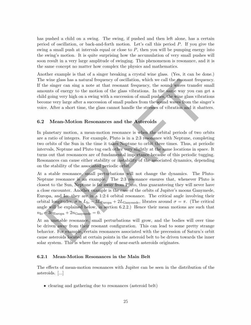
Figure 17: Histogram of semimajor axes of 298,000 asteroids. Major Jovian mean-motionresonance locations are marked in red. The Trojan asteroids are in 1:1 resonance near 5.2AU, and the Hilda family of asteroids is stabilized by the 3:2 resonance near 3.9 AU.
26
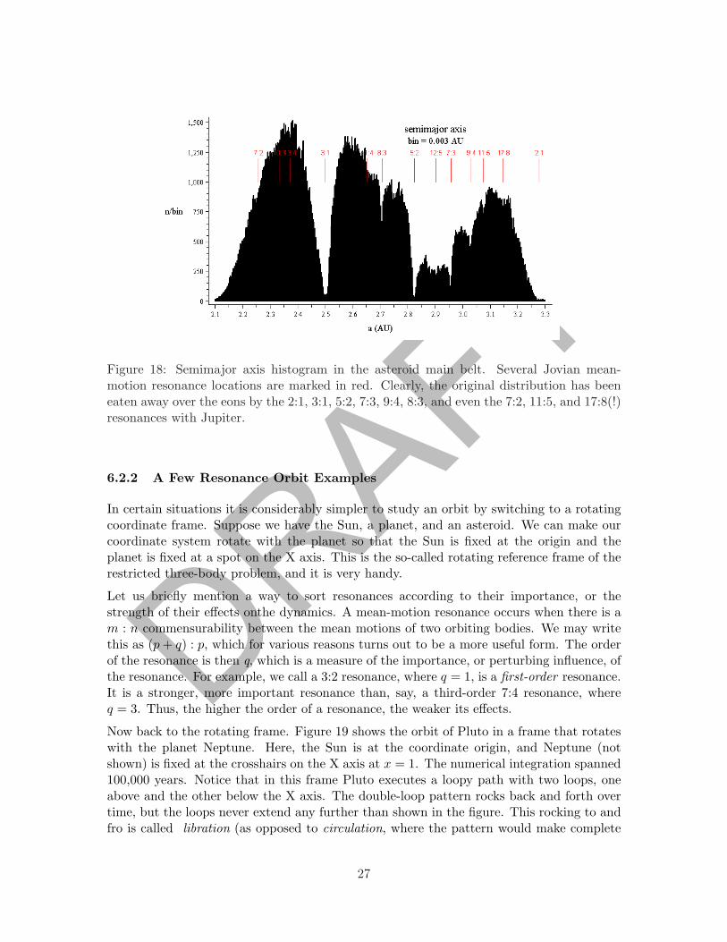
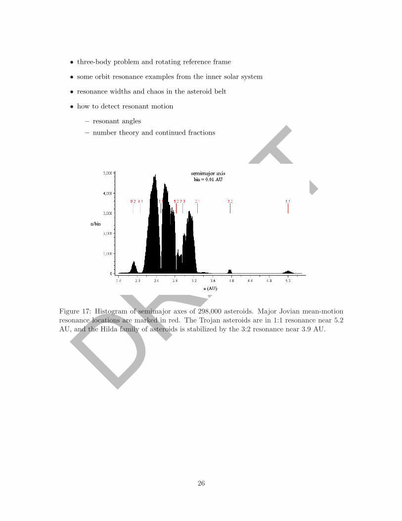
DRAFTFigure 18: Semimajor axis histogram in the asteroid main belt. Several Jovian mean-motion resonance locations are marked in red. Clearly, the original distribution has beeneaten away over the eons by the 2:1, 3:1, 5:2, 7:3, 9:4, 8:3, and even the 7:2, 11:5, and 17:8(!)resonances with Jupiter.
6.2.2 A Few Resonance Orbit Examples
In certain situations it is considerably simpler to study an orbit by switching to a rotatingcoordinate frame. Suppose we have the Sun, a planet, and an asteroid. We can make ourcoordinate system rotate with the planet so that the Sun is fixed at the origin and theplanet is fixed at a spot on the X axis. This is the so-called rotating reference frame of therestricted three-body problem, and it is very handy.
Let us briefly mention a way to sort resonances according to their importance, or thestrength of their effects onthe dynamics. A mean-motion resonance occurs when there is am : n commensurability between the mean motions of two orbiting bodies. We may writethis as (p + q) : p, which for various reasons turns out to be a more useful form. The orderof the resonance is then q, which is a measure of the importance, or perturbing influence, ofthe resonance. For example, we call a 3:2 resonance, where q = 1, is a first-order resonance.It is a stronger, more important resonance than, say, a third-order 7:4 resonance, whereq = 3. Thus, the higher the order of a resonance, the weaker its effects.
Now back to the rotating frame. Figure 19 shows the orbit of Pluto in a frame that rotateswith the planet Neptune. Here, the Sun is at the coordinate origin, and Neptune (notshown) is fixed at the crosshairs on the X axis at x = 1. The numerical integration spanned100,000 years. Notice that in this frame Pluto executes a loopy path with two loops, oneabove and the other below the X axis. The double-loop pattern rocks back and forth overtime, but the loops never extend any further than shown in the figure. This rocking to andfro is called libration (as opposed to circulation, where the pattern would make complete
27
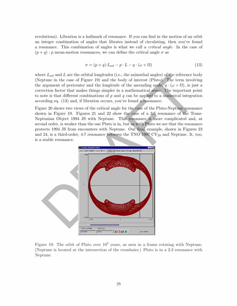
DRAFTrevolutions). Libration is a hallmark of resonance. If you can find in the motion of an orbitan integer combination of angles that librates instead of circulating, then you’ve founda resonance. This combination of angles is what we call a critical angle. In the case of(p + q) : p mean-motion resonances, we can define the critical angle σ as
σ = (p + q)·Lref − p · L− q · (ω + Ω) (13)
where Lref and L are the orbital longitudes (i.e., the azimuthal angles) of the reference body(Neptune in the case of Figure 19) and the body of interest (Pluto). The term involvingthe argument of pericenter and the longitude of the ascending node, q · (ω + Ω), is just acorrection factor that makes things simpler in a mathematical sense. The important pointto note is that different combinations of p and q can be applied to a numerical integrationaccording eq. (13) and, if libration occurs, you’ve found a resonance.
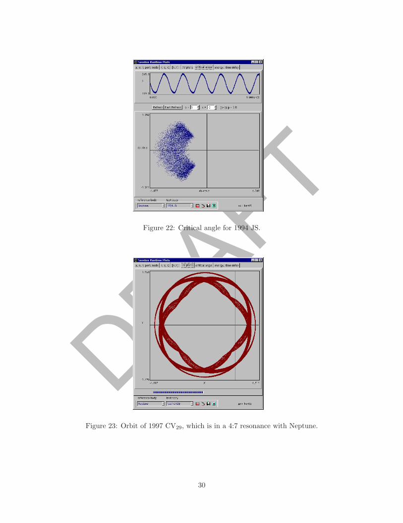
Figure 20 shows two views of the critical angle for the case of the Pluto-Neptune resonanceshown in Figure 19. Figures 21 and 22 show the case of a 3:5 resonance of the Trans-Neptunian Object 1994 JS with Neptune. This resonance is more complicated and, atsecond order, is weaker than the one Pluto is in, but as with Pluto we see that the resonanceprotects 1994 JS from encounters with Neptune. Our final example, shown in Figures 23and 24, is a third-order, 4:7 resonance between the TNO 1997 CV29 and Neptune. It, too,is a stable resonance.
Figure 19: The orbit of Pluto over 105 years, as seen in a frame rotating with Neptune.(Neptune is located at the intersection of the crosshairs.) Pluto is in a 2:3 resonance withNeptune.
28
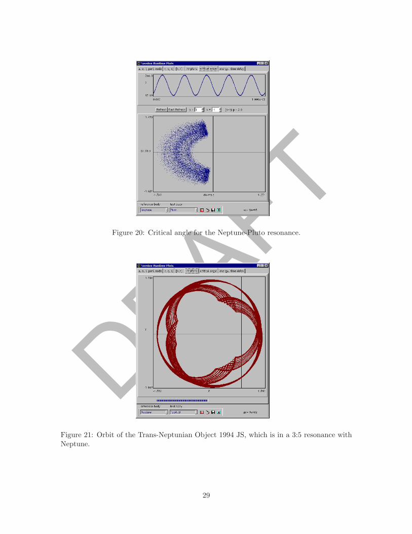
DRAFTFigure 20: Critical angle for the Neptune-Pluto resonance.
Figure 21: Orbit of the Trans-Neptunian Object 1994 JS, which is in a 3:5 resonance withNeptune.
29
DRAFTFigure 22: Critical angle for 1994 JS.
Figure 23: Orbit of 1997 CV29, which is in a 4:7 resonance with Neptune.
30
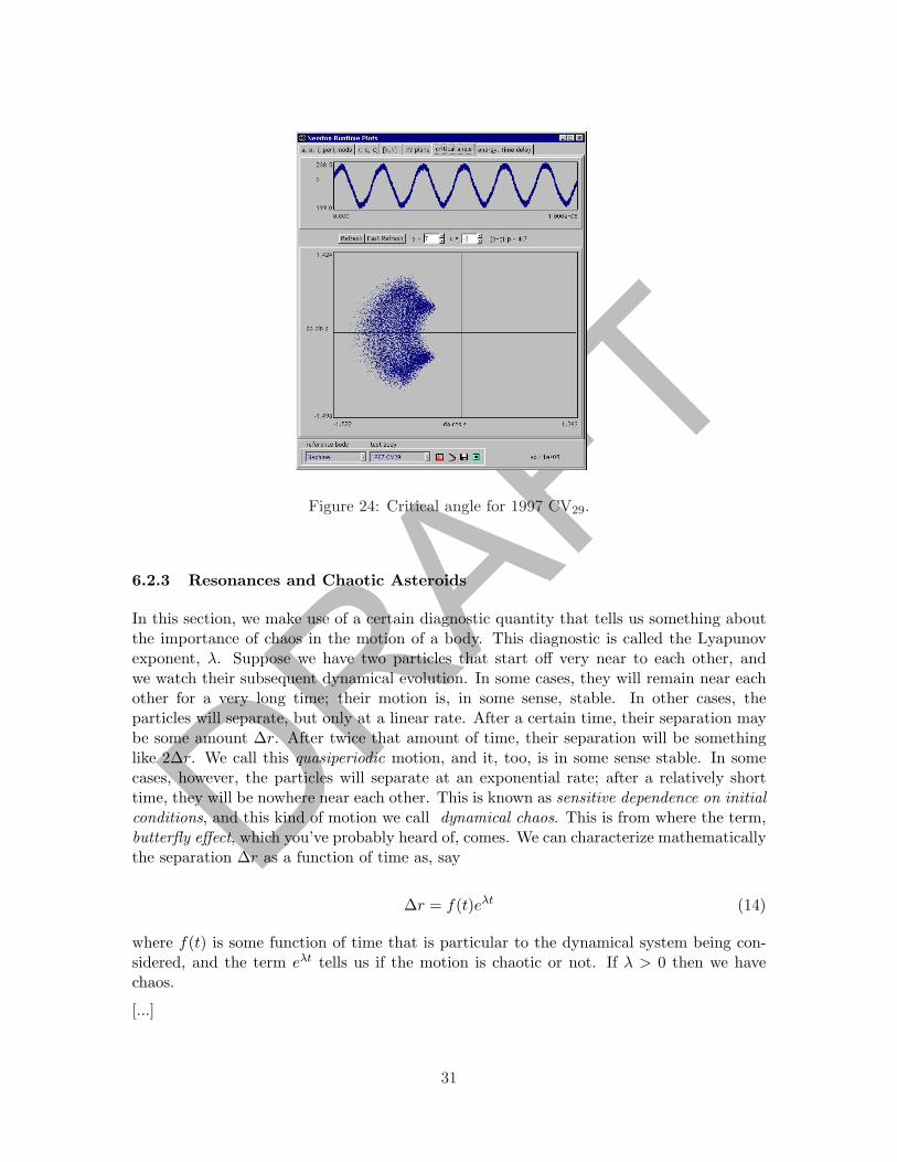
DRAFTFigure 24: Critical angle for 1997 CV29.
6.2.3 Resonances and Chaotic Asteroids
In this section, we make use of a certain diagnostic quantity that tells us something aboutthe importance of chaos in the motion of a body. This diagnostic is called the Lyapunovexponent, λ. Suppose we have two particles that start off very near to each other, andwe watch their subsequent dynamical evolution. In some cases, they will remain near eachother for a very long time; their motion is, in some sense, stable. In other cases, theparticles will separate, but only at a linear rate. After a certain time, their separation maybe some amount ∆r. After twice that amount of time, their separation will be somethinglike 2∆r. We call this quasiperiodic motion, and it, too, is in some sense stable. In somecases, however, the particles will separate at an exponential rate; after a relatively shorttime, they will be nowhere near each other. This is known as sensitive dependence on initialconditions, and this kind of motion we call dynamical chaos. This is from where the term,butterfly effect, which you’ve probably heard of, comes. We can characterize mathematicallythe separation ∆r as a function of time as, say
∆r = f(t)eλt (14)
where f(t) is some function of time that is particular to the dynamical system being con-sidered, and the term eλt tells us if the motion is chaotic or not. If λ > 0 then we havechaos.
[...]
31
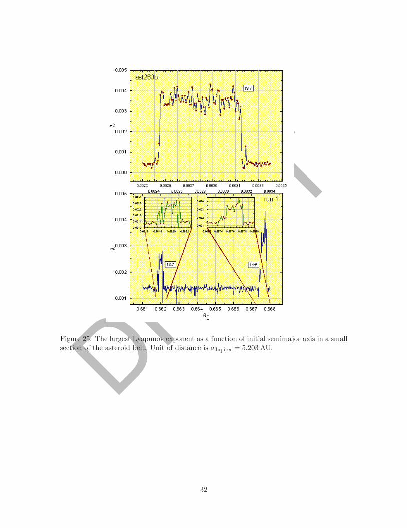
DRAFTFigure 25: The largest Lyapunov exponent as a function of initial semimajor axis in a smallsection of the asteroid belt. Unit of distance is aJupiter = 5.203 AU.
32
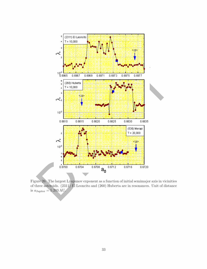
DRAFTFigure 26: The largest Lyapunov exponent as a function of initial semimajor axis in vicinitiesof three asteroids. (2311) El Leoncito and (260) Huberta are in resonances. Unit of distanceis aJupiter = 5.203 AU.
33
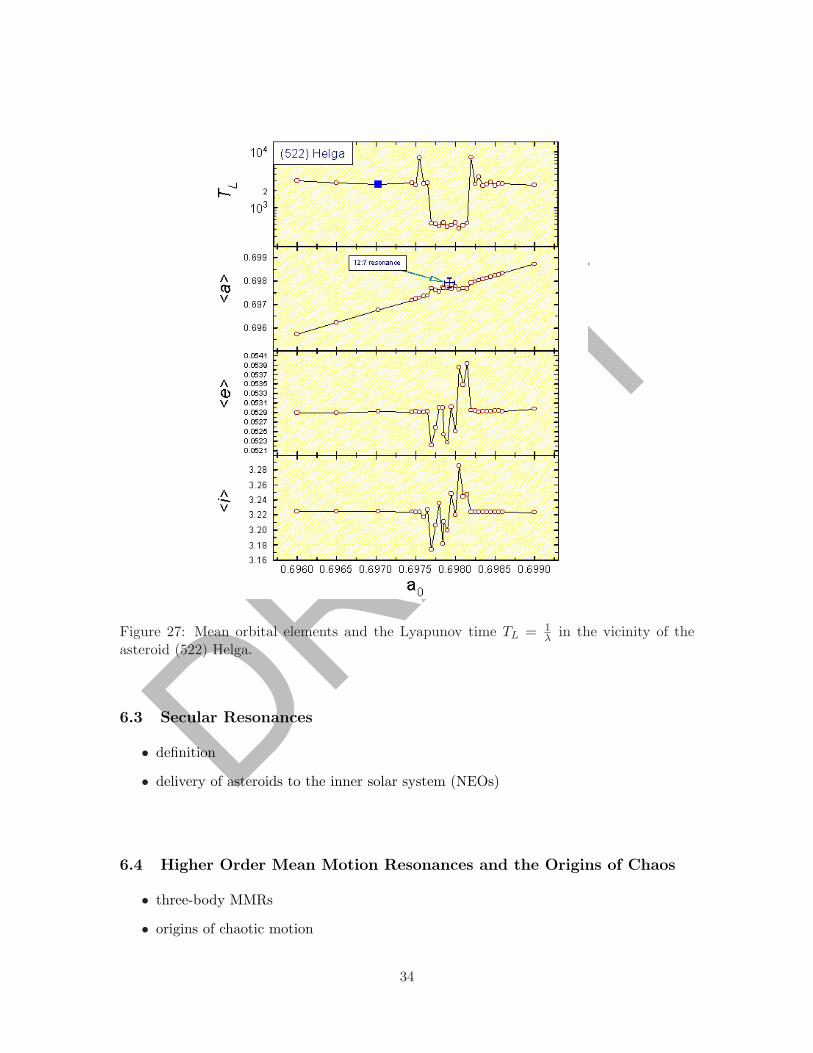
DRAFTFigure 27: Mean orbital elements and the Lyapunov time TL = 1
λ in the vicinity of theasteroid (522) Helga.
6.3 Secular Resonances
• definition
• delivery of asteroids to the inner solar system (NEOs)
6.4 Higher Order Mean Motion Resonances and the Origins of Chaos
• three-body MMRs
• origins of chaotic motion
34
DRAFT7 Asteroid Noise
“The stars make no noise.” —Irish Saying
7.1 Two Kinds of Noise
Usually, when we think of noise, it has some unpleasant connotation. This is true in physicsas it is in ordinary life. Noise invades every measurement – it is often very difficult tomitigate, and it is the ultimate barrier to the knowledge we seek from our measurements.Measurement noise is ordinarily most unwanted.
In addition to polluting measurements, noise is an intrinsic part of many physical processes.For example, you are probably familiar with the term random walk, which describes noiseof a specific kind. The buffeting that a particular molecule receives from its neighbors in agas or a liquid imparts just such a random walk to the molecule’s motion. This is known asBrownian motion, and it has certain characteristics, such as the fact that the distributionof lengths of the short segments that make up its motion is Gaussian. There are othertypes of noise – Poisson noise, white noise, red noise, 1/f noise, etc. – with correspondinglydifferent mathematical functions that characterize their distributions. Hence, we may turnthe tables and, instead of cursing, use measurements of physical process noise to learnsomething about the system we’re measuring. (We will still curse at measurement noise,alas.)
Taking a cue from the notion of process noise, we may adopt a somewhat unconventionalview of planetary motions in the Solar System. Consider the simple, idealized two-body
35
DRAFTproblem, a planet and the Sun. The planet’s path in space is smooth and predictable.Now add another planet. Its presence will perturb the first planet’s motion. Its path willstill be smooth, but characterization and prediction in detail starts to become considerablymore difficult. Continue adding perturbing masses, and the path in space, at small scales,becomes increasingly “wiggly” and unpredictable. The deviations from simple two-bodymotion begin to look more and more like process noise.
Now consider the planets of the inner solar system: Mercury through Mars. Their mo-tions are perturbed by each other and by the outer planets, especially by massive (but,fortunately for us, distant) Jupiter. This web of perturbations certainly greatly complicatestheir individual paths through space. But not only are there the other planets, there arein addition hundreds of thousands of the small bodies we call asteroids. Now, the massesof individual asteroids are very small compared to the planets. However, their masses, in-dividually and collectively, do affect planetary motions at length scales of order kilometersor less. Since there are many asteroids, the gravitational buffeting to which the inner solarsystem planets are subjected is, from a measurement perspective, indistinguishable fromnoise. Using Newton’s equations of motion, we may explore and characterize the effects of“asteroid noise” on the motions of the planets. First, however, we should look at just whatthe distribution of the asteroids is, because that is the primary noise source, so to speak.We cannot understand the consequences of noise if we do not first understand the noisesource itself.
7.2 The Asteroid Mass Distribution
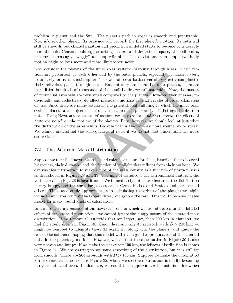
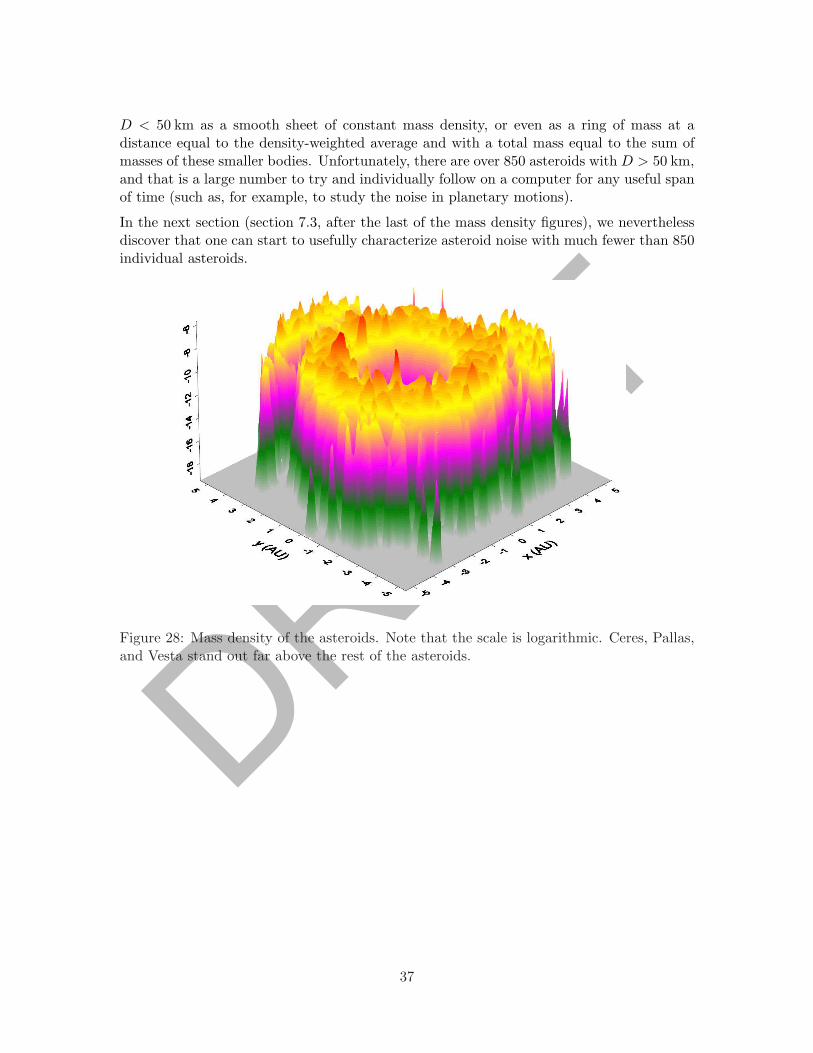
Suppose we take the known asteroids and calculate masses for them, based on their observedbrightness, their distance, and the fraction of sunlight that reflects from their surfaces. Wecan use this information to make a plot of the mass density as a function of position, suchas that shown in Figures 28 and 29. The unit of distance is the astronomical unit, and thevertical scale in Fig. 28 is logarithmic. We immediately notice two features: the distributionis very lumpy, and the three largest asteroids, Ceres, Pallas, and Vesta, dominate over allothers. Thus, as a crude approximation in calculating the orbits of the planets we mightinclude just Ceres, or just the largest three, and ignore the rest. This would be a servicablemodel for many useful kinds of calculation.
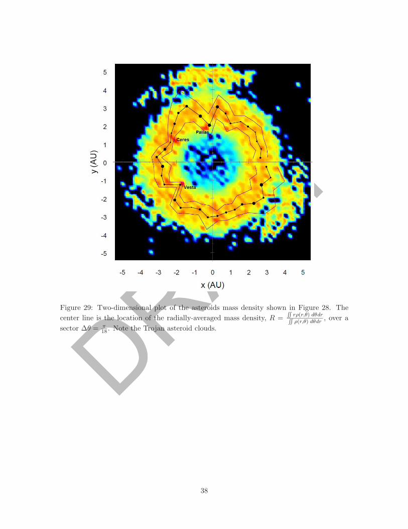
In a more accurate consideration, however – one in which we are interested in the detailedeffects of the asteroid population – we cannot ignore the lumpy nature of the asteroid massdistribution. If we remove all asteroids that are larger, say, than 200 km in diameter, wefind the result shown in Figure 30. Since there are only 31 asteroids with D > 200 km, wemight be tempted to integrate those 31 explicitly, along with the planets, and ignore therest of the asteroids, hoping that this model will give a good approximation of the asteroidnoise in the planetary motions. However, we see that the distribution in Figure 30 is alsovery uneven and lumpy. If we make the size cutoff 100 km, the leftover distribution is shownin Figure 31. We are starting to see some smoothing of the distribution, but it is still farfrom smooth. There are 264 asteroids with D > 100 km. Suppose we make the cutoff at 50km in diameter. The result is Figure 32, where we see the distribution is finally becomingfairly smooth and even. In this case, we could then approximate the asteriods for which
36
DRAFTD < 50 km as a smooth sheet of constant mass density, or even as a ring of mass at adistance equal to the density-weighted average and with a total mass equal to the sum ofmasses of these smaller bodies. Unfortunately, there are over 850 asteroids with D > 50 km,and that is a large number to try and individually follow on a computer for any useful spanof time (such as, for example, to study the noise in planetary motions).
In the next section (section 7.3, after the last of the mass density figures), we neverthelessdiscover that one can start to usefully characterize asteroid noise with much fewer than 850individual asteroids.
Figure 28: Mass density of the asteroids. Note that the scale is logarithmic. Ceres, Pallas,and Vesta stand out far above the rest of the asteroids.
37
DRAFTFigure 29: Two-dimensional plot of the asteroids mass density shown in Figure 28. Thecenter line is the location of the radially-averaged mass density, R =
˜rρ(r,θ) dθdr˜ρ(r,θ) dθdr
, over asector ∆θ = π
18 . Note the Trojan asteroid clouds.
38
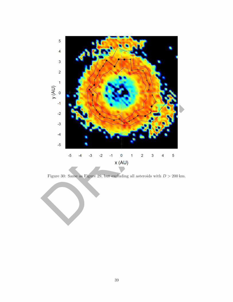
DRAFTFigure 30: Same as Figure 29, but excluding all asteroids with D > 200 km.
39
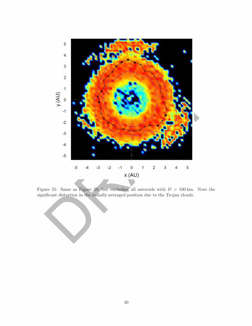
DRAFTFigure 31: Same as Figure 29, but excluding all asteroids with D > 100 km. Note thesignificant distortion in the radially-averaged position due to the Trojan clouds.
40
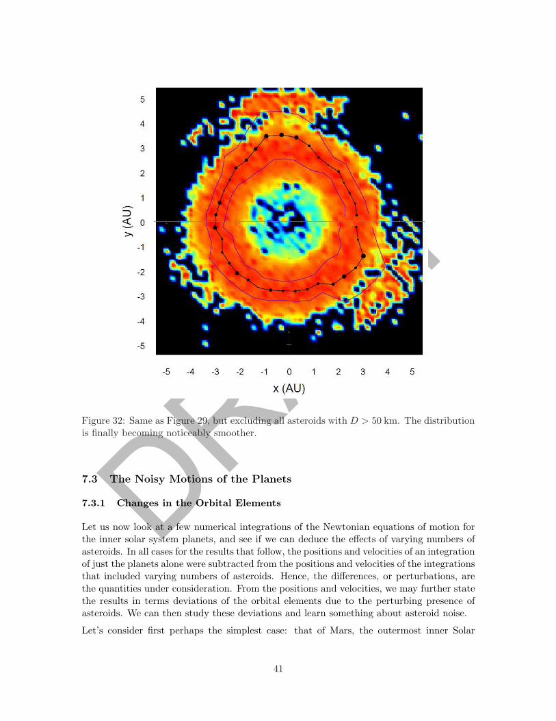
DRAFTFigure 32: Same as Figure 29, but excluding all asteroids with D > 50 km. The distributionis finally becoming noticeably smoother.
7.3 The Noisy Motions of the Planets
7.3.1 Changes in the Orbital Elements
Let us now look at a few numerical integrations of the Newtonian equations of motion forthe inner solar system planets, and see if we can deduce the effects of varying numbers ofasteroids. In all cases for the results that follow, the positions and velocities of an integrationof just the planets alone were subtracted from the positions and velocities of the integrationsthat included varying numbers of asteroids. Hence, the differences, or perturbations, arethe quantities under consideration. From the positions and velocities, we may further statethe results in terms deviations of the orbital elements due to the perturbing presence ofasteroids. We can then study these deviations and learn something about asteroid noise.
Let’s consider first perhaps the simplest case: that of Mars, the outermost inner Solar
41
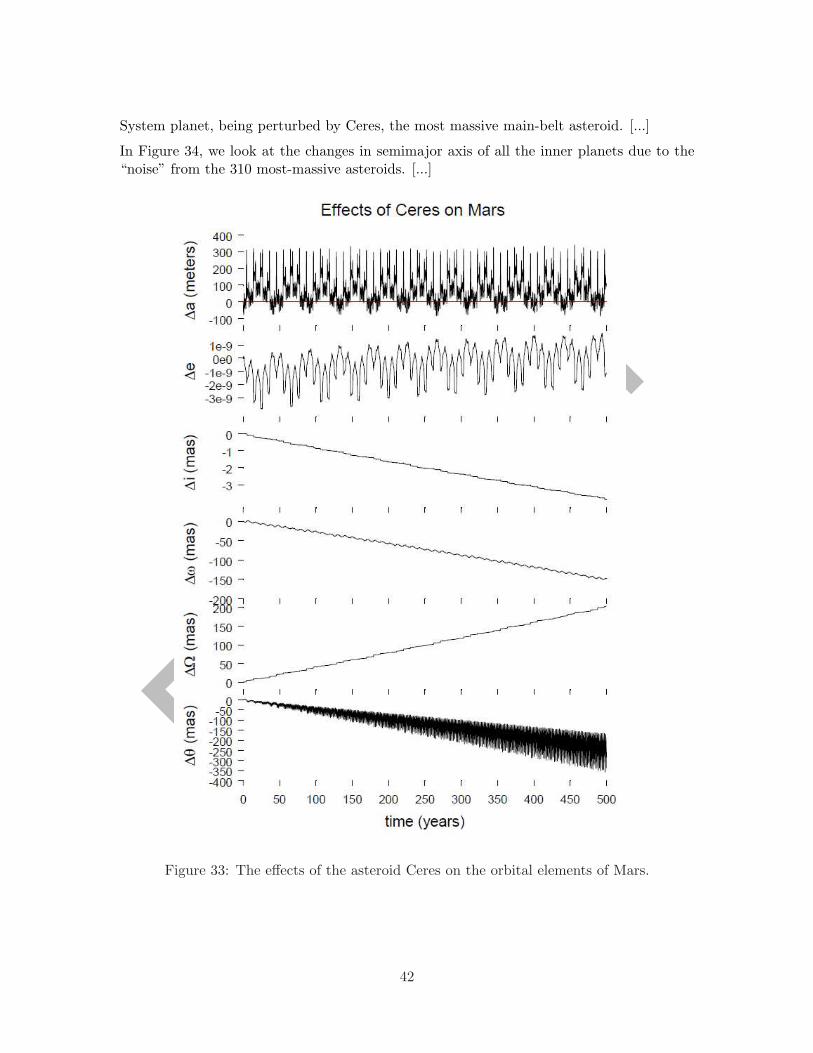
DRAFTSystem planet, being perturbed by Ceres, the most massive main-belt asteroid. [...]
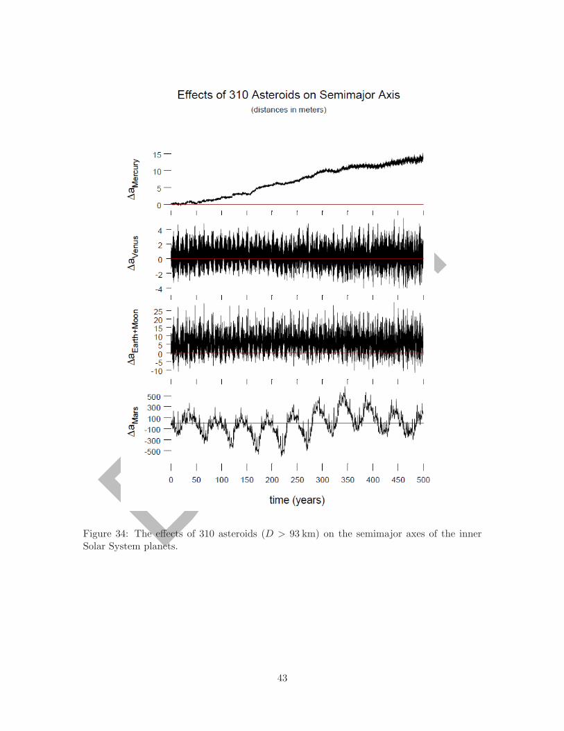
In Figure 34, we look at the changes in semimajor axis of all the inner planets due to the“noise” from the 310 most-massive asteroids. [...]
Figure 33: The effects of the asteroid Ceres on the orbital elements of Mars.
42
DRAFT
Figure 34: The effects of 310 asteroids (D > 93 km) on the semimajor axes of the innerSolar System planets.
43
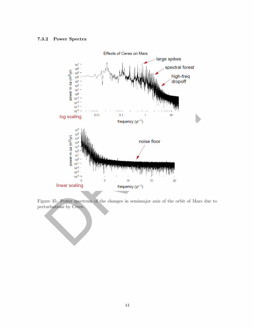
DRAFT7.3.2 Power Spectra
Figure 35: Power spectrum of the changes in semimajor axis of the orbit of Mars due toperturbations by Ceres.
44
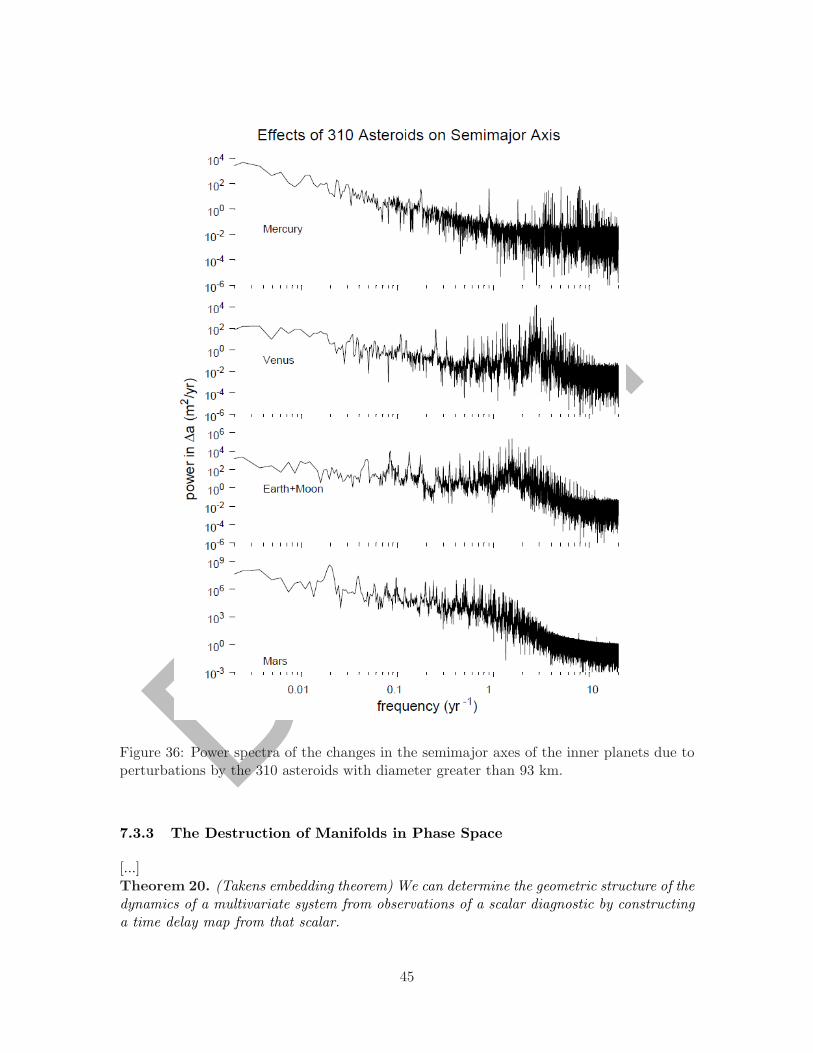
DRAFT
Figure 36: Power spectra of the changes in the semimajor axes of the inner planets due toperturbations by the 310 asteroids with diameter greater than 93 km.
7.3.3 The Destruction of Manifolds in Phase Space
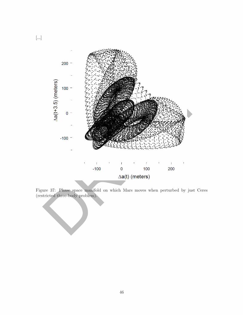
[...]Theorem 20. (Takens embedding theorem) We can determine the geometric structure of thedynamics of a multivariate system from observations of a scalar diagnostic by constructinga time delay map from that scalar.
45
DRAFT[...]
Figure 37: Phase space manifold on which Mars moves when perturbed by just Ceres(restricted three-body problem).
46
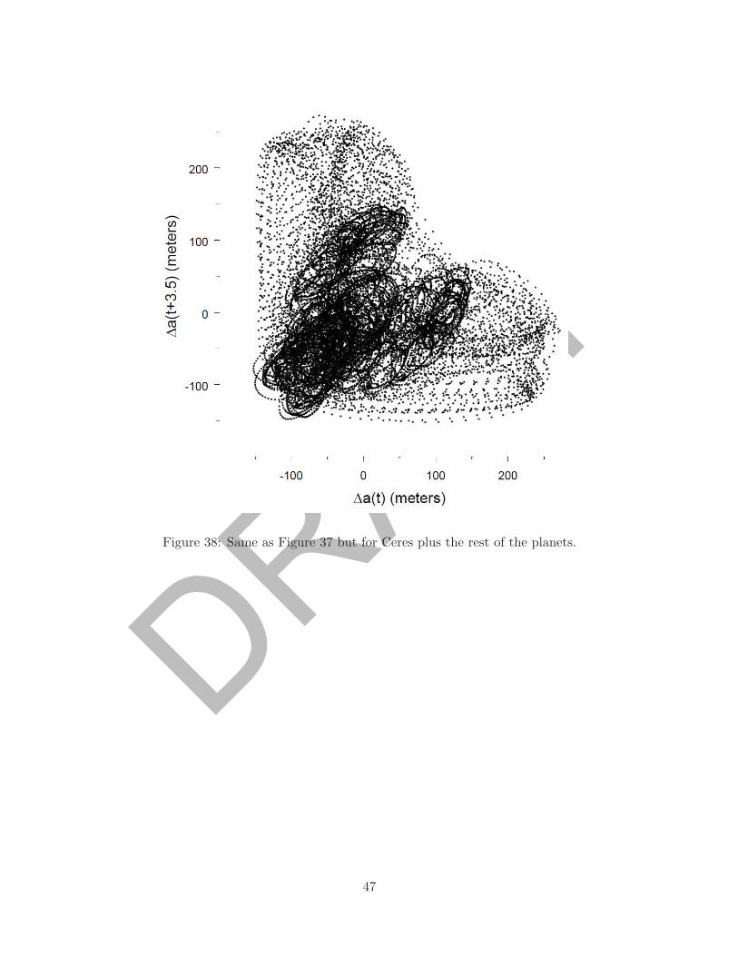
DRAFTFigure 38: Same as Figure 37 but for Ceres plus the rest of the planets.
47
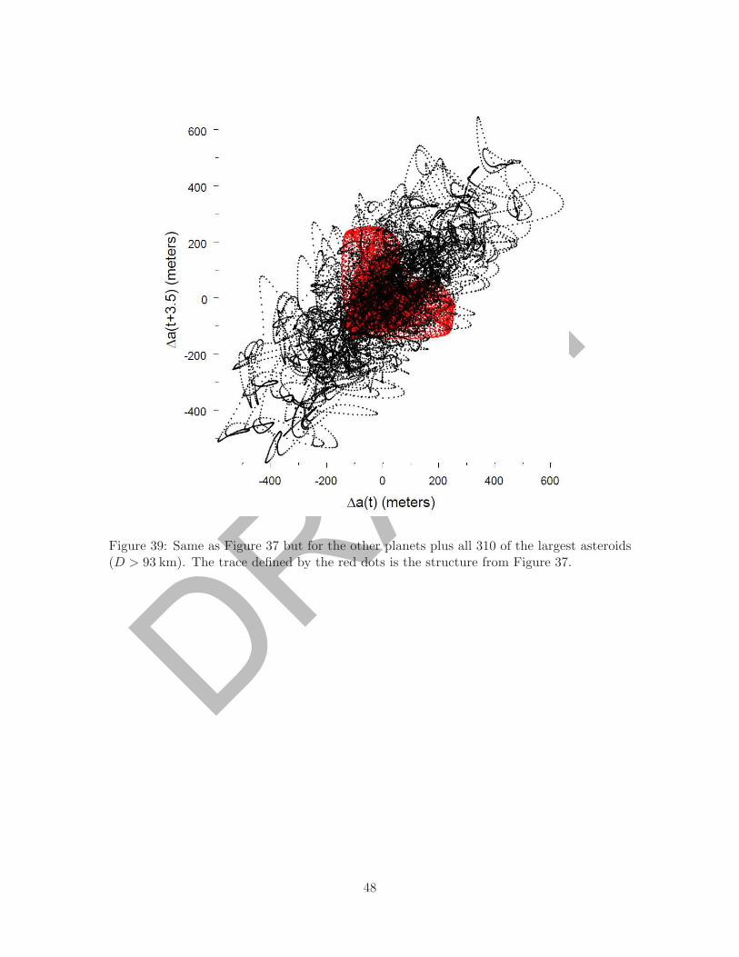
DRAFTFigure 39: Same as Figure 37 but for the other planets plus all 310 of the largest asteroids(D > 93 km). The trace defined by the red dots is the structure from Figure 37.
48

DRAFT
49