Embed Size (px)
Citation preview

An Introduction toConfiguration Interaction Theory
C. David Sherrill
School of Chemistry and Biochemistry
Georgia Institute of Technology
1995

CONTENTS 2
Contents
1 Introduction 4
2 Fundamental Concepts 7
2.1 Scope of the Method . . . . . . . . . . . . . . . . . . . . . . . . . . . 7
2.2 Why Configuration Interaction? . . . . . . . . . . . . . . . . . . . . . 8
2.3 The Correlation Energy . . . . . . . . . . . . . . . . . . . . . . . . . . 11
2.4 Slater’s Rules . . . . . . . . . . . . . . . . . . . . . . . . . . . . . . . 13
3 The Variational Theorem 15
3.1 The Method of Linear Variations . . . . . . . . . . . . . . . . . . . . . 15
3.2 Variational Theorem for the Ground State . . . . . . . . . . . . . . . . 17
3.3 Why are Coupled-Cluster and MBPT Energies not Variational? . . . . . 18
3.4 Application of the Variational Theorem to Other States . . . . . . . . . 19
3.5 Convergence of the Wavefunction . . . . . . . . . . . . . . . . . . . . 20
3.6 Variational Theorem Bounds on Excited States . . . . . . . . . . . . . 20
4 Reducing the CI Space 21
4.1 Symmetry Restrictions on the CI Space . . . . . . . . . . . . . . . . . 21
4.2 Classification of Basis Functions by Excitation Level . . . . . . . . . . 23
4.3 Energy Contributions of the Various Excitation Levels . . . . . . . . . . 24
4.4 Size of the CI Space as a Function of Excitation Level . . . . . . . . . . 25
4.5 The Frozen Core Approximation . . . . . . . . . . . . . . . . . . . . . 27

4.6 Truncated CI is not Size Extensive . . . . . . . . . . . . . . . . . . . . 31
5 Second Quantization 34
6 Determinant CI 37
6.1 Introduction to Determinant CI . . . . . . . . . . . . . . . . . . . . . . 37
6.2 Alpha and Beta Strings . . . . . . . . . . . . . . . . . . . . . . . . . . 37
6.2.1 Graphical Representation of Alpha and Beta Strings . . . . . . 39
6.3 RAS CI . . . . . . . . . . . . . . . . . . . . . . . . . . . . . . . . . . 45
6.3.1 Olsen’s Full CI σ Equations . . . . . . . . . . . . . . . . . . . 46
6.4 Full CI Algorithm . . . . . . . . . . . . . . . . . . . . . . . . . . . . . 51

1 INTRODUCTION 4
1 Introduction and Notation
These notes attempt to present the essential ideas of configuration interaction (CI) the-
ory in a fairly detailed mathematical framework. Of all the ab initio methods, CI is
probably the easiest to understand—and perhaps one of the hardest to implement effi-
ciently on a computer! The next two sections explain what the CI method is: the matrix
formulation of the Schrodinger equation HΨ = EΨ. The remaining sections describe
various simplifications, approximations, and computational techniquies.
I have attempted to use a uniform notation throughout these notes. Much of the
notation is consistent with that of Szabo and Ostlund, Modern Quantum Chemistry [1].
Below are listed several of the commonly-used symbols and their meanings.
N The number of electrons in the system.
nα The number of alpha electrons.
nβ The number of beta electrons.
n The number of orbitals in the one-particle basis set.
δij Kronecker delta function, equal to one if i = j and zero otherwise.
H The exact nonrelativistic Hamiltonian operator.
H The Hamiltonian matrix, i.e. the matrix form of H , in whatever N -electron basis is
currently being used.
Hij The i, j-th element of H, equal to 〈Φi|H|Φj〉, where Φi and Φj are N -electron CI
basis functions.
xi The space and spin coordinates of particle i.
ri The spatial coordinates of particle i.
φi The i-th one-particle basis function (orbital). Usually denotes a spin-orbital obtained
from a Hartree-Fock procedure. May also be written simply as i.
1 INTRODUCTION 5
χi The i-th one-particle basis function (orbital). Usually denotes an atomic spin-orbital.
|Φi〉 The i-th N -electron basis function. Usually denotes a single Slater determinant,
but may also be a configuration state function (CSF).
|Ψ〉 Usually denotes an eigenfunction of H. The exact nonrelativistic wavefunction if
a complete basis is used in the expansion of H .
|Φra〉 An N -electron basis function which differs from some reference function |Φ0〉 by
the replacement of spin-orbital a by spin-orbital r. Usually implies a single Slater
determinant.
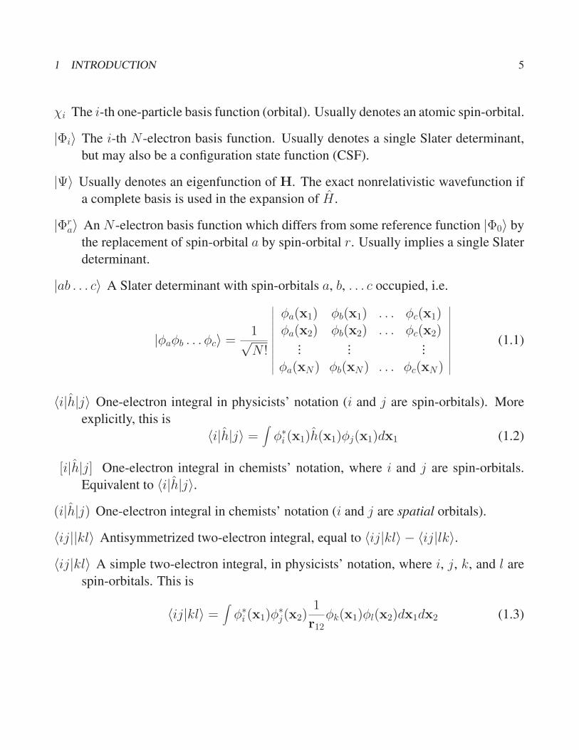
|ab . . . c〉 A Slater determinant with spin-orbitals a, b, . . . c occupied, i.e.
|φaφb . . . φc〉 =1√N !
∣
∣
∣
∣
∣
∣
∣
∣
∣
∣
∣
∣
φa(x1) φb(x1) . . . φc(x1)φa(x2) φb(x2) . . . φc(x2)
......
...
φa(xN) φb(xN) . . . φc(xN)
∣
∣
∣
∣
∣
∣
∣
∣
∣
∣
∣
∣
(1.1)
〈i|h|j〉 One-electron integral in physicists’ notation (i and j are spin-orbitals). More
explicitly, this is
〈i|h|j〉 =∫
φ∗i (x1)h(x1)φj(x1)dx1 (1.2)
[i|h|j] One-electron integral in chemists’ notation, where i and j are spin-orbitals.
Equivalent to 〈i|h|j〉.
(i|h|j) One-electron integral in chemists’ notation (i and j are spatial orbitals).
〈ij||kl〉 Antisymmetrized two-electron integral, equal to 〈ij|kl〉 − 〈ij|lk〉.
〈ij|kl〉 A simple two-electron integral, in physicists’ notation, where i, j, k, and l are
spin-orbitals. This is
〈ij|kl〉 =∫
φ∗i (x1)φ
∗j(x2)
1
r12φk(x1)φl(x2)dx1dx2 (1.3)
1 INTRODUCTION 6
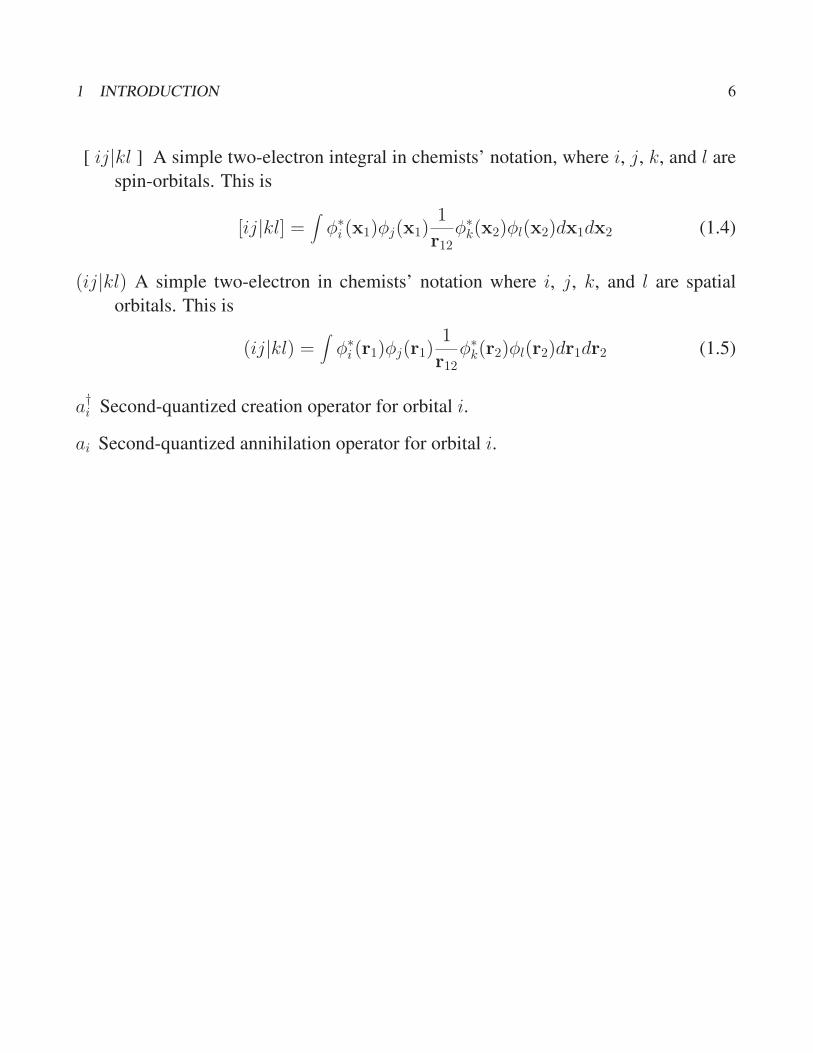
[ ij|kl ] A simple two-electron integral in chemists’ notation, where i, j, k, and l are
spin-orbitals. This is
[ij|kl] =∫
φ∗i (x1)φj(x1)
1
r12φ∗k(x2)φl(x2)dx1dx2 (1.4)
(ij|kl) A simple two-electron in chemists’ notation where i, j, k, and l are spatial
orbitals. This is
(ij|kl) =∫
φ∗i (r1)φj(r1)
1
r12φ∗k(r2)φl(r2)dr1dr2 (1.5)
a†i Second-quantized creation operator for orbital i.
ai Second-quantized annihilation operator for orbital i.
2 FUNDAMENTAL CONCEPTS 7
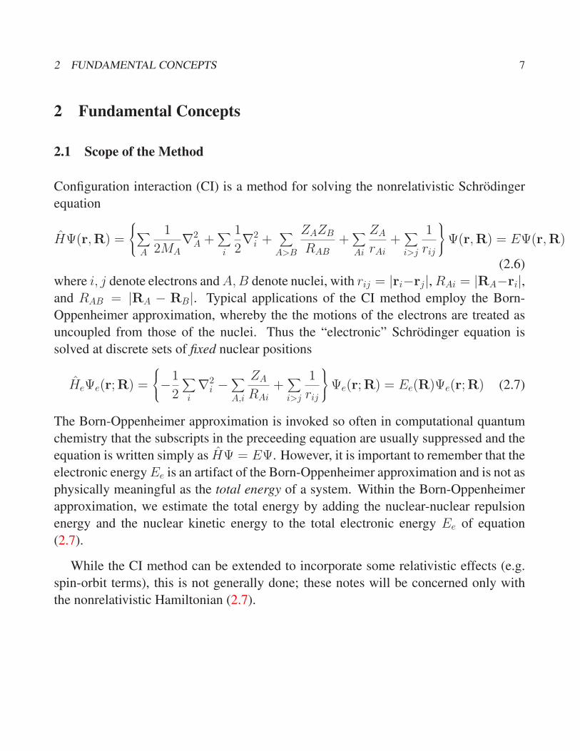
2 Fundamental Concepts
2.1 Scope of the Method
Configuration interaction (CI) is a method for solving the nonrelativistic Schrodinger
equation
HΨ(r,R) =
∑
A
1
2MA∇2
A +∑
i
1
2∇2
i +∑
A>B
ZAZB
RAB+
∑
Ai
ZA
rAi+
∑
i>j
1
rij
Ψ(r,R) = EΨ(r,R)
(2.6)
where i, j denote electrons and A,B denote nuclei, with rij = |ri−rj|, RAi = |RA−ri|,and RAB = |RA − RB|. Typical applications of the CI method employ the Born-
Oppenheimer approximation, whereby the the motions of the electrons are treated as
uncoupled from those of the nuclei. Thus the “electronic” Schrodinger equation is
solved at discrete sets of fixed nuclear positions
HeΨe(r;R) =
−1
2
∑
i
∇2i −
∑
A,i
ZA
RAi+
∑
i>j
1
rij
Ψe(r;R) = Ee(R)Ψe(r;R) (2.7)
The Born-Oppenheimer approximation is invoked so often in computational quantum
chemistry that the subscripts in the preceeding equation are usually suppressed and the
equation is written simply as HΨ = EΨ. However, it is important to remember that the
electronic energy Ee is an artifact of the Born-Oppenheimer approximation and is not as
physically meaningful as the total energy of a system. Within the Born-Oppenheimer
approximation, we estimate the total energy by adding the nuclear-nuclear repulsion
energy and the nuclear kinetic energy to the total electronic energy Ee of equation
(2.7).
While the CI method can be extended to incorporate some relativistic effects (e.g.
spin-orbit terms), this is not generally done; these notes will be concerned only with
the nonrelativistic Hamiltonian (2.7).

2 FUNDAMENTAL CONCEPTS 8
2.2 Why Configuration Interaction?
In the first paper on quantum mechanics, Heisenberg used matrix mechanics to cal-
culate the frequencies and intensities of spectral lines [2]. Later, when Schrodinger
discovered wave mechanics, it was quickly shown that the Schrodinger and Heisenberg
approaches are mathematically equivalent [3, 4]. Given the ease with which matrices
may be implemented on a computer, it is entirely natural to attempt to solve the molec-
ular time-independent Schrodinger equation HΨ = EΨ using matrix mechanics.
Matrix mechanics requires that we choose a vector space for the expansion of the
problem. For the case of an N -electron molecule, our wavefunction must be expanded
in a basis of N -particle functions (the nuclei need not be considered in the electronic
wavefunction, if we have invoked the Born-Oppenheimer approximation). How do we
construct the N -particle basis functions? Here we follow the arguments of Szabo and
Ostlund [1], p. 60. Assume we have a complete set of functions {χi(x1)} of a single
variable x1. Then any arbitrary function of that variable can be expanded exactly as
Φ(x1) =∑
i
aiχi(x1). (2.1)
How can we expand a function of two variables x1 and x2 which have the same domain?
If we hold x2 fixed, then
Φ(x1, x2) =∑
i
ai(x2)χi(x1). (2.2)
Now note that each expansion coefficient ai(x2) is a function of a single variable, which
can be expanded as
ai(x2) =∑
j
bijχj(x2). (2.3)
Substituting this expression into the one for Φ(x1, x2), we now have
Φ(x1, x2) =∑
ij
bijχi(x1)χj(x2) (2.4)
a process which can obviously be extended for Φ(x1, x2, . . . , xN).

2 FUNDAMENTAL CONCEPTS 9
Let us now collect the spin and space coordinates of an electron into a variable x.
We can write a spin orbital as χ(x). The result analogous to equation (2.4) for a system
of N electrons is
Φ(x1,x2, . . . ,xN) =∑
ij...N
bij...Nχi(x1)χj(x2) . . . χN(xN) (2.5)
However, the wavefunction must be antisymmetric with respect to the exchange of the
coordinates of any two electrons1 For the two-particle case, the requirement
Φ(x1,x2) = −Φ(x2,x1) (2.6)
implies that bij = −bji and bii = 0, or
Φ(x1,x2) =∑
j>i
bij[χi(x1)χj(x2)− χj(x1)χi(x2)]
=∑
j>i
21/2bij|χiχj〉 (2.7)
More generally, an arbitrary N -electron wavefunction can be expressed exactly as a lin-
ear combination of all possible N -electron Slater determinants formed from a complete
set of spin orbitals {χi(x)}. If we solve the matrix mechanics problem H|Ψ〉 = E|Ψ〉in a complete basis of N -electron functions as just described, we will obtain all elec-
tronic eigenstates of the system exactly. If our N -electron basis functions are denoted
|Φi〉, the eigenvectors of H are given as
|Ψj〉 =I∑
i
cij|Φi〉 (2.8)
if there are I possible N -electron basis functions (I will be infinite if we actually have
a complete set of one electron functions χi). The matrix H is constructed so that Hij =〈Φi|H|Φj〉 for i, j = 1, 2, . . . , I . The matrix elements Hij may be written in terms of
one- and two-electron integrals according to “Slater’s rules,” as discussed in section
2.4.
The N -electron basis functions |Φi〉 can be written as substitutions or “excitations”
from the Hartree-Fock “reference” determinant, i.e.
|Ψ〉 = c0|Φ0〉+∑
racra|Φr
a〉+∑
a<b,r<s
crsab|Φrsab〉+
∑
r<s<t,a<b<c
crstabc|Φrstabc〉+ . . . (2.9)
1According to the antisymmetry principle for fermions, of which the Pauli principle is a direct result.
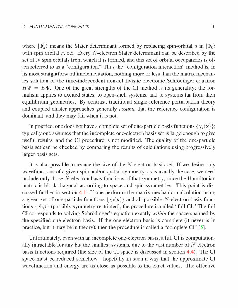
2 FUNDAMENTAL CONCEPTS 10
where |Φra〉 means the Slater determinant formed by replacing spin-orbital a in |Φ0〉
with spin orbital r, etc. Every N -electron Slater determinant can be described by the
set of N spin orbitals from which it is formed, and this set of orbital occupancies is of-
ten referred to as a “configuration.” Thus the “configuration interaction” method is, in
its most straightforward implementation, nothing more or less than the matrix mechan-
ics solution of the time-independent non-relativistic electronic Schrodinger equation
HΨ = EΨ. One of the great strengths of the CI method is its generality; the for-
malism applies to excited states, to open-shell systems, and to systems far from their
equilibrium geometries. By contrast, traditional single-reference perturbation theory
and coupled-cluster approaches generally assume that the reference configuration is
dominant, and they may fail when it is not.
In practice, one does not have a complete set of one-particle basis functions {χi(x)};
typically one assumes that the incomplete one-electron basis set is large enough to give
useful results, and the CI procedure is not modified. The quality of the one-particle
basis set can be checked by comparing the results of calculations using progressively
larger basis sets.
It is also possible to reduce the size of the N -electron basis set. If we desire only
wavefunctions of a given spin and/or spatial symmetry, as is usually the case, we need
include only those N -electron basis functions of that symmetry, since the Hamiltonian
matrix is block-diagonal according to space and spin symmetries. This point is dis-
cussed further in section 4.1. If one performs the matrix mechanics calculation using
a given set of one-particle functions {χi(x)} and all possible N -electron basis func-
tions {|Φi〉} (possibly symmetry-restricted), the procedure is called “full CI.” The full
CI corresponds to solving Schrodinger’s equation exactly within the space spanned by
the specified one-electron basis. If the one-electron basis is complete (it never is in
practice, but it may be in theory), then the procedure is called a “complete CI” [5].
Unfortunately, even with an incomplete one-electron basis, a full CI is computation-
ally intractable for any but the smallest systems, due to the vast number of N -electron
basis functions required (the size of the CI space is discussed in section 4.4). The CI
space must be reduced somehow—hopefully in such a way that the approximate CI
wavefunction and energy are as close as possible to the exact values. The effective
2 FUNDAMENTAL CONCEPTS 11
reduction of the CI space is a major concern in CI theory, and we will discuss some of
the more popular approaches in these notes.
By far the most common CI approximation is the truncation of the CI space ex-
pansion according to excitation level relative to the reference state (equation 2.9). The
widely-employed CI singles and doubles (CISD) wavefunction includes only those N -
electron basis functions which represent single or double excitations relative to the
reference state. Since the Hamiltonian operator includes only one- and two-electron
terms, only singly and doubly excited configurations can interact directly with the ref-
erence, and they typically account for about 95% of the correlation energy in small
molecules at their equilibrium geometries [6]. Truncation of the CI space according to
excitation class is discussed more thoroughly in section 4.2.
2.3 The Correlation Energy
Approximate CI methods can be judged according to what fraction of the correlation
energy they recover. The correlation energy is defined as the difference between the
energy in the Hartree-Fock limit (EHF ) and the exact nonrelativistic energy of a system
(E0)Ecorr = E0 − EHF (2.10)
This energy will always be negative because the Hartree-Fock energy is an upper bound
to the exact energy (this is guaranteed by the variational theorem, as explained in sec-
tion 3). The exact nonrelativistic energy E0 could, in principle, be calculated by per-
forming a full CI in a complete one-electron basis set. If we have an incomplete one-
electron basis set, then we can only compute the basis set correlation energy, which
is the correlation energy for a given one-electron basis. For convenience, the basis set
correlation energy is often simply referred to as the correlation energy.
The correlation energy is the energy recovered by fully allowing the electrons to
avoid each other; Hartree-Fock improperly treats interelectron repulsions in an aver-
aged way.2 However, there is some inconsistency in this line of thinking. When a
2Some texts talk about the “average” electron repulsion term in the Fock operator; I find this misleading in that Hartree-

2 FUNDAMENTAL CONCEPTS 12
molecule is pulled apart, the electrons shouldn’t need to avoid each other as much, so
the magnitude of the correlation energy should decrease. In fact, the opposite is true, as
shown by the basis set correlation energies given in Table 1 for H2O at three different
geometries.
Table 1: Electron Correlation in H2O with a DZ Basis.
Geometry Ecorr (hartree)a
Re -0.148028
1.5 Re -0.210992
2.0 Re -0.310067aData from reference [6].
The correlation energy increases at stretched geometries, because our definition of
the correlation energy in equation (2.10) includes not only the concept of electrons
avoiding each other, which is called the “dynamical” correlation energy, but also a more
subtle effect called the “nondynamical,” or “static” correlation energy. Nondynamical
correlation energy reflects the inadequacy of a single reference in describing a given
molecular state, and is due to nearly degenerate states or rearrangement of electrons
within partially filled shells. Shavitt [7] has pointed out this deficiency in the defini-
tion of the correlation energy, and has suggested that perhaps a multiconfigurational
Hartree-Fock method may be more useful in the definition of correlation energy.
Siegbahn [8] offers the following explanation of the difference between dynamical
and nondynamical correlation energies:
“In many situations it is further convenient to subdivide the correlation
energy into two parts with different physical origins. For chemical reactions
where bonds are broken and formed, and for most excited states, the ma-
jor part of the correlation energy can be obtained by adding only a few extra
configurations besides the Hartree-Fock configuration. This part of the corre-
lation energy is due to near degeneracy between different configurations and
Fock uses the same instantaneous interelectron repulsion term as CI—it’s the same Hamiltonian! The restriction to a single
Slater determinant is what causes the averaging of interelectron repulsions.
2 FUNDAMENTAL CONCEPTS 13
has its origin quite often in artifacts of the Hartree-Fock approximation. The
physical origin of the second part of the correlation energy is the dynamical
correlation of the motion of the electrons and is therefore sometimes called
the dynamical correlation energy. Since the Hamiltonian operator contains
only one- and two-particle operators this part of the correlation energy can
be very well described by single and double replacements from the leading,
near degenerate, reference configurations.”
2.4 Slater’s Rules
Whether we perform a full CI or only a limited CI, we must be able to express H in
matrix form so that we can diagonalize it and obtain the eigenvectors and eigenvalues of
interest. In this section we discuss Slater’s rules (or the Slater-Condon rules [9, 10, 11]),
which allow us to express matrix elements Hij = 〈Φi|H|Φj〉 in terms of one- and two-
electron integrals. At the moment, we will express these results in terms spin-orbitals
using physicist’s notation. The one-electron integrals are written as
〈i|h|j〉 =∫
φ∗i (r1)h(r1)φj(r1)dr1 (2.11)
and the two-electron integrals are written as
〈ij||kl〉 = 〈ij|kl〉 − 〈ij|lk〉 (2.12)
where
〈ij|kl〉 =∫
φ∗i (r1)φ
∗j(r2)
1
r12φk(r1)φl(r2)dr1dr2 (2.13)
Before Slater’s rules can be used, the two Slater determinants must be arranged in
maximum coincidence. Remember that switching columns in a determinant introduces
a minus sign. For instance, to calculate 〈Φ1|H|Φ2〉, where we have
|Φ1〉 = |abcd〉 (2.14)
|Φ2〉 = |crds〉 (2.15)

2 FUNDAMENTAL CONCEPTS 14
then we must first interchange columns of |Φ1〉 or |Φ2〉 to make the two determinants
look as much alike as possible. For example, we may rearrange |Φ2〉 as
|Φ2〉 = |crds〉 = −|crsd〉 = |srcd〉 (2.16)
After the determinants are in maximum coincidence, we see how many spin orbitals
they differ by, and we then use the following rules:
1. Identical Determinants: If the determinants are identical, then
〈Φ1|H|Φ1〉 =N∑
m〈m|h|m〉+
N∑
m>n〈mn||mn〉 (2.17)
2. Determinants that Differ by One Spin Orbital:
|Φ1〉 = | · · ·mn · · ·〉 (2.18)
|Φ2〉 = | · · · pn · · ·〉
〈Φ1|H|Φ2〉 = 〈m|h|p〉+N∑
n〈mn||pn〉
3. Determinants that Differ by Two Spin Orbitals:
|Φ1〉 = | · · ·mn · · ·〉 (2.19)
|Φ2〉 = | · · · pq · · ·〉〈Φ1|H|Φ2〉 = 〈mn||pq〉
4. Determinants that differ by More than Two Spin Orbitals:
|Φ1〉 = | · · ·mno · · ·〉 (2.20)
|Φ2〉 = | · · · pqr · · ·〉〈Φ1|H|Φ2〉 = 0
The derivation of these rules can be found in Szabo and Ostlund [1], section 2.3.4
(pp. 74-81).
3 THE VARIATIONAL THEOREM 15
3 The Variational Theorem
3.1 The Method of Linear Variations
In this section we show that the method of linear variations (also called the Ritz method
[12]) is equivalent to the matrix formulation Hc = Ec of the Schrodinger equation
H|Ψ〉 = E|Ψ〉. Our treatment is similar to that of Szabo and Ostlund [1], p. 116. The
linear variation method states that, given the linear expansion
|Ψ〉 = ∑
i
ci|Φi〉 (3.1)
we vary the coefficients ci so that we minimize E = 〈Ψ|H|Ψ〉/〈Ψ|Ψ〉. We begin
by requiring that the wavefunction be normalized so that 〈Ψ|Ψ〉 = 1. Normalization
means that we cannot minimize E simply by solving
δ
δck〈Ψ|H|Ψ〉 = 0 k = 1, 2, . . . , N (3.2)
because the ci’s are not independent. In this case we have a constrained minimization,
so we apply Lagrange’s method of undetermined multipliers, and we minimize the
functional
L = 〈Ψ|H|Ψ〉 − E(〈Ψ|Ψ〉 − 1) (3.3)
which has the same minimum as E when |Ψ〉 is normalized. When we substitute equa-
tion (3.1) into equation (3.3), we obtain
L =∑
ij
c∗i cj〈Φi|H|Φj〉 − E
∑
ij
c∗i cj〈Φi|Φj〉 − 1
(3.4)
which we may rewrite as
L =∑
ij
c∗i cjHij − E
∑
ij
c∗i cjSij − 1
(3.5)
where of course Hij = 〈Φi|H|Φj〉 and Sij = 〈Φi|Φj〉. Now set the first variation in Lequal to zero:
δL =∑
ij
δc∗i cjHij − E∑
ij
δc∗i cjSij +∑
ij
c∗i δcjHij − E∑
ij
c∗i δcjSij = 0 (3.6)
3 THE VARIATIONAL THEOREM 16
Since the summations run over all i and j, and since Hij = H∗ji and Sij = S∗
ji, we can
simplify to
δL =∑
i
δc∗i
∑
j
Hijcj − ESijcj
+ complex conj. = 0 (3.7)
Since each term is a sum of a number and its complex conjugate, the imaginary parts
will cancel. However, the real part will not necessarily be zero; in fact, since all the
δci’s are arbitrary (that is the whole point of using Lagrange’s method), then for δL to
be zero, the term in brackets must be zero. We may rewrite this condition as a matrix
equation
Hc = ESc (3.8)
If the basis functions { |Φi〉 } are chosen orthonormal (as is usually the case), then
S = I the identity matrix, and we have Hc = Ec. Of course c is the column-vector
representation of |Ψ〉 in the basis { |Φi〉 }. We thus have two equivalent ways of viewing
a CI—either as the matrix formulation of the Schrodinger equation within the given
linear vector space of N -electron basis functions, or as the minimization of the energy
with respect to the linear expansion coefficients ci of (3.1), subject to the constraint
that the wavefunction remain normalized. Another way of viewing the results of this
section is to note that only eigenvectors of the Hamiltonian matrix H are stable with
respect to variations in the linear expansion coefficients.
At this point it is reasonable to ask why we wish to minimize the energy by varying
the coefficients in equation (3.1). How do we know that this will give us the best
estimate of the wavefunction? There are two answers to this. First, as we have just
shown, minimizing the energy by variation of the linear expansion coefficients gives the
Schrodinger equation in matrix form; thus the procedure is justified a posteriori by the
validity of its result. The other reason is that, for the ground state, the linear expansion
in equation (3.1) gives an expectation value for the energy E which is always an upper
bound to the exact nonrelativistic ground state energy E0. We will prove this assertion
in the next section; the result is called the Variational Theorem. The best estimate of
E, then, is the minimum value which can be obtained by varying the coefficients in
equation (3.1) (while also maintaining normalization). These arguments also hold for
excited states, so long as each excited state is made orthogonal to all lower states.

3 THE VARIATIONAL THEOREM 17
3.2 Variational Theorem for the Ground State
One particularly nice feature of the CI method is that the calculated lowest energy
eigenvalue is always an upper bound to the exact ground state energy. Our approxi-
mate wavefunction |Θ〉 can always be expressed as a linear combination of the exact
nonrelativistic eigenvectors |Ψi〉, which span the entire N -electron space.
|Θ〉 = ∑
i
ci|Ψi〉 (3.9)
and the energy is given by
E =〈Θ|H|Θ〉〈Θ|Θ〉 (3.10)
Now if |Θ〉 is normalized, and we substitue the expansion over exact eigenfunctions
(equation 3.9) into the equation above, we obtain
E =∑
i
c∗i ciEi (3.11)
where Ei is the ith energy eigenvalue, i.e. H|Ψi〉 = Ei|Ψi〉. Now subtract E0, the exact
nonrelativistic ground state energy, from both sides to obtain
E − E0 =∑
i
c∗i ciEi − E0 (3.12)
or
E − E0 =∑
i
c∗i ci(Ei − E0) (3.13)
since |Θ〉 is normalized and∑
i c∗i ci = 1. Since Ei are greater than or equal to E0 for
all values of i and the coefficients c∗i ci are necessarily non-negative, the right hand side
of equation (3.12) is non-negative, so that E ≥ E0. We should also point out that the
variational theorem holds for the Hartree-Fock method as well as for CI, since equation
(3.10) is valid for the Hartree-Fock energy—for a given set of MO’s, the HF energy
can be formulated as a (trivial) 1 x 1 CI eigenvalue problem. In a similar manner, the
MCSCF method (where MO’s and CI coefficients are optimized) is also “variational.”
It should be clear that instead of using the exact nonrelativistic eigenfunctions |Ψi〉in equation (3.9), we could also have used an expansion over the exact eigenfunctions

3 THE VARIATIONAL THEOREM 18
within the one-electron space spanned by |Θ〉 (i.e. we could expand the approximate CI
wavefunction |Θ〉 in terms of the full CI wavefunctions). This means that not only is
the approximate energy an upper bound to the exact nonrelativistic ground-state energy,
but it is also an upper bound to the full CI energy in the given one-electron basis.
3.3 Why are Coupled-Cluster and MBPT Energies not Variational?
Electron correlation methods other than CI may not be variational. For example, con-
sider the coupled-cluster energy expression
E =〈Φ0|e−THeT |Φ0〉
〈Φ0|Φ0〉(3.14)
If the operator eT is not trunctated, then we know that eT |Φ0〉 = |Ψ0〉. Generally,
however, the operator is truncated. Let us define eT′|Φ0〉 = |ΘA〉 for our truncated T ′.
Now define 〈Φ0|e−T ′
= 〈ΘB|. Note that in general |ΘB〉 6= |ΘA〉, which would have
occurred had we used 〈Φ0|(eT ′
)† on the left. Then the energy expression is
E =〈ΘB|H|ΘA〉〈Φ0|Φ0〉
(3.15)
which, after expansion over the complete set of eigenvectors, becomes
E =
∑
ij c∗idj〈Ψi|H|Ψj〉〈Φ0|Φ0〉
(3.16)
This simplifies to
E =
∑
i c∗idiEi
〈Φ0|Φ0〉(3.17)
At this point we can go no farther, because the terms c∗idi may be negative, in contrast
to the situation in equation (3.12).
For completeness, we also show that MBPT energies are not variational. The nth
order MBPT wavefunction may be written [13] as
|Θ(n)MBPT〉 = |Φ0〉+
n∑
k=1
V(1− |Φ0〉〈Φ0|)E0 −H0
k
|Φ0〉L (3.18)

3 THE VARIATIONAL THEOREM 19
where the sum is over “linked diagrams” only. The nth order energy is then given by
E(n)MBPT = 〈Φ0|H|Θ(n−1)
MBPT〉 (3.19)
Since this integral is not symmetric, the energy is not variational. Only the first-order
perturbation theory energy (which is also the Hartree-Fock energy) is variational, since
it uses |Θ(0)MBPT〉 = |Φ0〉.
3.4 Application of the Variational Theorem to Other States
In this section, we parallel the arguments of Pauling and Wilson [14], p. 186. So far,
we have shown only that the energy calculated as the expectation value of some trial
function must be an upper bound to the true ground state energy E0. In certain cases,
we may derive a similar result for other states. If we take a trial function |Φ0〉 such that
the first k coefficients in equation (3.9) are zero, then we may subtract Ek from equation
(3.11) to obtain
E − Ek =∑
i
c∗i ci(Ei − Ek) (3.20)
Now since we’ve assumed cj = 0, j = 0, 1, . . . , k, this simplifies to
E − Ek =∑
i=k
c∗i ci(Ei − Ek) (3.21)
Once again, we can see that every term on the right side is nonnegative, so E−Ek ≥ 0.
There are any number of cases in which we have a trial function of the form just de-
scribed. Consider, for example, a calculation on a triplet state for a molecule which has
a singlet ground state. If our trial function is constrained to be a triplet, then all singlet
eigenfunctions |Ψi〉 will have zero coefficients in the expansion of the trial function. In
this case, the energy we minimize from the triplet trial function will be an upper bound
to the lowest triplet energy, even though there is a lower-lying singlet state. Similar
arguments can be made for spatial symmetry.

3 THE VARIATIONAL THEOREM 20
3.5 Convergence of the Wavefunction
A consequence of the variational theorem is that as the energy E of an approximate
variational wavefunction approaches the exact energy E0, the approximate wavefunc-
tion |Φ〉 approaches the exact one |Ψ0〉. This follows from equation (3.12), which
shows that as the energy E is minimized (or, equivalently, as E − E0 is minimized),
then∑
i c∗i ci(Ei − E0) is minimized; that is, the sum of squares of the absolute values
of the coefficients of excited states with weight factors (Ei − E0) is minimized. It is
apparent that these weight factors might not be optimal if we want the |Φ〉 which gives
the best value for a property other than the energy, such as dipole moment. However,
in the limit that E is minimized with a sufficiently large basis so that E = E0, then∑
i=1 c∗i ci(Ei − E0) = 0, or c0 = 1, implying that |Φ〉 = |Ψ0〉. Once we have the exact
wavefunction, then of course all properties can be computed exactly (again, within the
Born-Oppernheimer approximation and neglecting relativistic effects). To summarize,
variational improvements in the energy give improvements in the approximate wave-
function, which in turn improves the values of all other properties; however, these other
properties will not necessarily converge as fast as the energy with respect to N -electron
basis set improvement.
3.6 Variational Theorem Bounds on Excited States
Just as the lowest eigenvalue has been shown to be an upper bound to the exact ground-
state energy, more generally, any eigenvalue Ei can be shown to be an upper bound to
the corresponding exact excited state energy Ei [15]. In fact, one can also show that as
other N -electron basis functions are added to the CI procedure, the eigenvalues obey
the MacDonald-Hylleraas-Undheim relations [15, 16]
E(m)i−1 ≤ E
(m+1)i ≤ E
(m)i (3.22)
where m is the number of N -electron basis functions.

4 REDUCING THE CI SPACE 21
4 Reducing the Size of the CI Space
4.1 Symmetry Restrictions on the CI Space
In this section we discuss some general considerations concerning which N -electron
basis functions should be included in the CI space (given that, in the general case, there
are too many for us to include all of them). Certainly if we can find a class of N -
electron functions which rigorously have zero Hamiltonian matrix elements with the
desired CI wavefunction, then none of these basis functions will contribute at all to
our approximate wavefunction and they should not be included in the CI space; the
Hamiltonian will be block diagonal, and all the functions in this class will contribute
to the wrong block. We will now prove the following: consider an operator A which
commutes with H . If
A|Φ1〉 = a1|Φ1〉 (4.1)
and
A|Φ2〉 = a2|Φ2〉, a1 6= a2 (4.2)
then
〈Φ1|H|Φ2〉 = 0 (4.3)
First we show that H|Φ2〉 is an eigenfunction of A with eigenvalue a2. Define
H|Φ2〉 = |Φ′2〉 (4.4)
Now apply A to |Φ′2〉
A[
H|Φ2〉]
= AH|Φ2〉 (4.5)
= HA|Φ2〉= Ha2|Φ2〉= a2
[
H|Φ2〉]
Where we have used the given that AH = HA. We may now write
A|Φ′2〉 = a2|Φ′
2〉 (4.6)
4 REDUCING THE CI SPACE 22
Now consider again equation (4.1). If we take the adjoint of this equation we obtain
〈Φ1|A† = 〈Φ1|a∗1 (4.7)
Now use the fact that A = A† (we assumed A was Hermitian) and that the eigenvalues
of a Hermitian operator are real. This yields
〈Φ1|A = 〈Φ1|a1 (4.8)
Multiply on the right by |Φ′2〉
〈Φ1|A|Φ′2〉 = a1〈Φ1|Φ′
2〉 (4.9)
Now multiply equation (4.6) on the left by 〈Φ1| to obtain
〈Φ1|A|Φ′2〉 = a2〈Φ1|Φ′
2〉 (4.10)
If we subtract equation (4.10) from equation (4.9) we arrive at
(a1 − a2)〈Φ1|Φ′2〉 = 0 (4.11)
Since we assumed a1 6= a2, then 〈Φ1|Φ′2〉 = 0. Recalling the definition of |Φ′
2〉, we
have
〈Φ1|H|Φ2〉 = 0 (4.12)
which was to be proven. Thus if our desired wavefunction is an eigenfunction of some
Hermitian operator that commutes with the Hamiltonian, our CI space need not include
those N -electron functions which are eigenfunctions of this operator with different
eigenvalues. As an example, consider the spin angular momentum operator S2. If we
want to solve for a state |Ψ〉 of spin S, then we know
S2|Ψ〉 = S(S + 1)|Ψ〉 (4.13)
and any basis function of a different spin can be excluded from the CI. Slater determi-
nants are generally not eigenfunctions of S2. However, we can take linear combinations
of Slater determinants so that we do have eigenfunctions of S2; such functions are gen-
erally called configuration state functions, or CSF’s. The advantage of using CSF’s is
that we can throw out all functions with the wrong eigenvalue S—they contribute to

4 REDUCING THE CI SPACE 23
another, noninteracting block of the Hamiltonian matrix. This reasoning also applies
to symmetry operations of point groups, such that we can throw away any N -electron
basis functions (whether determinants or CSF’s) which have the wrong irreducible rep-
resentation. We can also restrict the basis functions according to their eigenvalues with
respect to the operator Sz. For a triplet state, we can perform the calculation using
basis functions which have Ms = −1, 0, or 1. If we were to include basis functions
of all these values of Ms, we would obtain a triply-degenerate answer—as one should
expect!3
4.2 Classification of Basis Functions by Excitation Level
Now we will discuss the importance of various excitation classes to the CI wavefunc-
tion. As noted in equation (2.9), the CI expansion is typically truncated according
to excitation level; in the vast majority of CI studies, the expansion is truncated (for
computational tractability) at doubly-excited configurations. Since the Hamiltonian
contains only two-body terms, only singles and doubles can interact directly with the
reference (for the sake of simplicity, we are assuming only a single reference for now).
This is a direct result of Slater’s Rules (cf. section 2.4). The structure of the CI ma-
trix with respect to excitation level is given below (adapted from Szabo and Ostlund
[1], p. 235), where |S〉, |D〉, |T 〉, and |Q〉 represent blocks of singly, doubly, triply,
and quadruply excited determinants, respectively. The Hamiltonian matrix H is Hermi-
tian; if only real orbitals are used, as is usually the case, then the Hamiltonian is also
symmetric. Thus only the lower triangle of H is shown below.
H =
〈Φ0|〈S|〈D|〈T |〈Q|
...
〈Φ0|H|Φ0〉 · · ·0 〈S|H|S〉 · · ·
〈D|H|Φ0〉 〈D|H|S〉 〈D|H|D〉 · · ·0 〈T |H|S〉 〈T |H|D〉 〈T |H|T 〉 · · ·0 0 〈Q|H|D〉 〈Q|H|T 〉 〈Q|H|Q〉 · · ·...
......
......
...
(4.14)
3However, state-of-the-art determinant-based CI algorithms often include computational simplifications if the Ms = 0component is used [17].
4 REDUCING THE CI SPACE 24
Note that the matrix elements 〈S|H|Φ0〉 are given as 0. This is due to Brillouin’s the-
orem, which is valid when our reference function |Φ0〉 is obtained by the Hartree-Fock
method (Hartree-Fock guarantees that off-diagonal elements of the Fock matrix are
zero, and it turns out that the matrix element between two Slater determinants which
differ by one spin orbital is equal to an off-diagonal element of the Fock matrix). Fur-
thermore, the blocks 〈X|H|Y 〉 which are not necessarily zero may still be sparse; for
example, the matrix element 〈Φrsab|H|Φtuvw
cdef 〉, which belongs to the block 〈D|H|Q〉, will
be nonzero only if a and b are contained in the set {c, d, e, f} and if r and s are con-
tained in the set {t, u, v, w}.
Since only the doubles interact directly with the Hartree-Fock reference, we expect
double excitations to make the largest contributions to the CI wavefunction, after the
reference state. Indeed, this is what is observed. Even though singles, triples, etc.
do not interact directly with the reference, they can still become part of the CI wave-
function (i.e. have non-zero coefficients) because they mix with the doubles, directly
or indirectly. Although singles are much less important to the energy than doubles,
they are generally included in CI treatments because of their relatively small number
and because of their greater importance in describing one-electron properties (dipole
moment, etc.)
4.3 Energy Contributions of the Various Excitation Levels
Table 2 demonstrates the importance of various excitation classes in obtaining CI en-
ergies. We see that singles and doubles account for 95% of the correlation energy at
the equilibrium geometries of the molecules listed. We see that quadruple excitations
are more important than triples, at least as far as the energy is concerned. At stretched
geometries, the CISD and CISDT methods become markedly poorer, yet the CISDTQ
method still recovers a very high (and nearly constant) fraction of the correlation en-
ergy, suggesting that CISDTQ should give reliable results for energy differences across
potential energy surfaces for molecules of this size.

4 REDUCING THE CI SPACE 25
Table 2: Percentage of correlation energy recovered by various CI excitation levels for some small
molecules.
Percent Corr. Energya
Molecule CISD CISDT CISDTQ
BH 94.91 n/a 99.97
H2O(Re) 94.70 95.47 99.82
H2O(1.5 Re) 89.39 91.15 99.48
H2O(2.0 Re) 80.51 83.96 98.60
NH3 94.44 95.43 99.84
HF 95.41 96.49 99.86
H+7 96.36 96.87 99.96
aData from reference [6] except for H+7 data
from reference [18].
4.4 Size of the CI Space as a Function of Excitation Level
We can also see from Table 3 that the number of N -electron basis functions increases
dramatically with increasing excitation level. It should be pointed out that while the
calculations on BH, HF, and H+7 used DZP basis sets, those on H2O and NH3 used only
DZ basis sets. A DZP basis should be considred the minimum adequate basis for a truly
meaningful benchmark study, and even then it is desirable to use a high-quality basis
such as an Atomic Natural Orbital (ANO) set. While it is generally possible to perform
CISD calculations on small molecules with a good one-electron basis, the CISDTQ
method is limited to molecules containing very few heavy atoms, due to the extreme
number of N -electron basis functions required. Full CI calculations are of course even
more difficult to perform, so that despite their importance as benchmarks, few full CI
energies using flexible one-electron basis sets have been obtained.
The size of the full CI space in CSF’s can be calculated (including spin symmetry
but ignoring spatial symmetry) by Weyl’s dimension formula as applied to the Distinct
row table (DRT). If N is the number of electrons, n is the number of orbitals, and S is

4 REDUCING THE CI SPACE 26
Table 3: Number of CSF’s required for small molecules at several levels of CI.
CSF’s requireda
Molecule CISD CISDT CISDTQ FCI
BH 568 n/a 28 698 132 686
H2O 361 3 203 17 678 256 473
NH3 461 4 029 19 925 137 321
HF 552 6 712 48 963 944 348
H+7 1 271 24 468 248 149 2 923 933
aData from reference [6] except for H+7 data from
reference [18].
the total spin, then the dimension of the CI space in CSF’s is given by
DnNS =2S + 1
n+ 1
n+ 1N/2− S
n+ 1N/2 + S + 1
(4.15)
The dimension of the full CI space in determinants (again, ignoring spatial symme-
try) is computed simply by
DnNαNβ=
nNα
nNβ
(4.16)
or, in a form closer to equation 4.15,
DnNS =
n
N/2 + S
n
N/2− S
(4.17)
Table 4 shows the dimension of the full CI space (neglecting spatial symmetry) in
determinants and in CSF’s. Current full CI algorithms are limited to a few million
determinants. Although there have been reports [19, 20, 21] of larger calculations (in-
cluding a few billion determinants), the computational expense is (currently) too great
for routine calculations of this size.

4 REDUCING THE CI SPACE 27
Table 4: Dimension of Full CI in Determinants (CSF’s in parentheses)
Number of electrons
Orbitals 6 8 10 12
10 14.4× 10³ 44.1× 10³ 63.5× 10³ 44.1× 10³
(4.95× 10³) (13.9× 10³) (19.4× 10³) (13.9× 10³)
20 1.30× 10⁶ 23.5× 10⁶ 240× 106 1.50× 10⁹
(379× 103) (5.80× 10⁶) (52.6× 10⁶) (300× 106)
30 16.5× 10⁶ 751× 106 20.3× 10⁹ 353× 109
(4.56× 10⁶) (172× 106) (4.04× 10⁹) (62.5× 10⁹)
4.5 The Frozen Core Approximation
It is quite common in applications of the CI method to invoke the frozen core ap-
proximation, in which the lowest-lying molecular orbitals (occupied by the inner-shell
electrons) are constrained to remain doubly-occupied in all configurations. The frozen
core for atoms lithium to neon typically consists of the 1s atomic orbital, while that
for atoms sodium to argon consists of the atomic orbitals 1s, 2s, 2px, 2py and 2pz. The
frozen molecular orbitals are those which are primarily these inner-shell atomic orbitals
(or linear combinations thereof).
A justification for this approximation is that the inner-shell electrons of an atom
are less sensitive to their environment than are the valence electrons. Thus the error
introduced by freezing the core orbitals is nearly constant for molecules containing the
same types of atoms. In fact, it is sometimes recommended that one employ the frozen
core approximation as a general rule because most of the basis sets commonly used in
quantum chemical calculations do not provide sufficient flexibility in the core region to
accurately describe the correlation of the core electrons.
Not only does the frozen core approximation reduce the number of configurations
in the CI procedure, but it also reduces the computational effort required to evaluate
matrix elements between the configurations which remain. Assuming that all frozen

4 REDUCING THE CI SPACE 28
core orbitals are doubly occupied and orthogonal to all other molecular orbitals, then it
can be shown [22] that
〈ΦI |H|ΦJ〉 = 〈ΦI |H0|ΦJ〉 (4.18)
where ΦI and ΦJ are identical to ΦI and ΦJ , respectively, except that the core orbitals
have been deleted from ΦI and ΦJ , and H has been replaced by H0 defined by
H0 = Ec +N−Nc∑
i=1
hc(i) +N−Nc∑
i>j
1
rij(4.19)
where N is the number of electrons and Nc is the number of core electrons. Ec is
the so-called “frozen-core energy,” which is the expectation value of the determinant
formed from only the Nc core electrons doubly occupying the nc = Nc/2 core orbitals
Ec = 2nc∑
i
hii +nc∑
ij
{2(ii|jj)− (ij|ji)} (4.20)
Finally, hc(i) is the one-electron Hamiltonian operator for electron i in the average field
produced by the Nc core electrons,
hc(i) = h(i) +nc∑
j=1
{
2Jj(i)− Kj(i)}
(4.21)
with Jj(i) and Kj(i) representing the standard Coulomb and exchange operators, re-
spectively. Note that, although we have written the frozen core energy Ec and frozen
core operator hc in terms of molecular orbitals, it is not necessary to explicitly transform
the one- and two-electron integrals involving core orbitals. Assuming real orbitals, we
can define a frozen core density matrix [23] in atomic (or symmetry) orbitals as
P cρσ =
nc∑
i
C iρC
iσ (4.22)
where C iρ is the contribution of atomic orbital ρ to molecular orbital i. Now the frozen
core operator in atomic orbitals becomes
hcµν = hµν + 2
∑
ρσ(ρσ|µν)P c
ρσ −∑
ρσ(ρµ|νσ)P c
ρσ (4.23)

4 REDUCING THE CI SPACE 29
and the frozen core operator in molecular orbitals hcij can be obtained simply by trans-
forming hcµν . Similarly the frozen core energy can be evaluated as
Ec =∑
µνP cµν
(
hµν + hcµν
)
(4.24)
= Tr(P ch) + Tr(P chc)
An analogous approximation is the deleted virtual approximation, whereby a few of
the highest-lying virtual (unoccupied) molecular orbitals are constrained to remain un-
occupied in all configurations. Since these orbitals can never be occupied, they can be
removed from the CI procedure entirely because no terms involving them contribute to
the CI coefficients or energy. The rationalization for this procedure is that it is unlikely
that electrons will choose to partially populate high-energy orbitals in their attempt to
avoid other electrons. However, this conclusion is generally true only for very high-
lying virtual orbitals (such as those formed by antisymmetric combinations of symme-
try orbitals in the core region). For all other virtual orbitals, such simplistic reasoning
is not sufficient.
Davidson points out that those high energy SCF virtual orbitals which result from the
antisymmetric combination of the two basis functions describing each atomic orbital in
a double-ζ basis set (such as the 3p-like orbital formed from the minus combination of
the larger and smaller 2p atomic orbitals on oxygen) often make the largest contribution
to the correlation energy in Møller-Plesset (MPn) wavefunctions [24]. This can be seen
from the expression for the second-order correction to the energy in Møller-Plesset
perturbation theory,
E(2) =∑
a>b
∑
r>s
|〈ab||rs〉|2ǫa + ǫb − ǫr − ǫs
(4.25)
where ǫi is the orbital energy (eigenvalue) of orbital i. Thus a virtual orbital r with a
large energy ǫr will contribute to a large energy denominator in each term of equation
(4.25) in which it appears. However, if orbital r lies close spatially to one of the orbitals
a or b occupied in the reference, then this large overlap will contribute to a large two-
electron integral 〈ab||rs〉. This integral is squared in the numerator, leading to a large
overall contribution to the second-order energy. For the antisymmetric combinations

4 REDUCING THE CI SPACE 30
of the basis functions describing the core region, this large numerator is insufficient to
overcome the even larger energy denominator; such virtual orbitals can generally be
deleted with minimal loss in the correlation energy recovered.
Although the analysis in the preceeding paragraph is based on perturbation theory,
similar conclusions can be drawn for the CI method. This is most easily verified by ac-
tual calculations, since analytical expressions for the energetic contribution of orbitals
to the CI energy are not nearly as simple to obtain or interpret as is equation (4.25).
4 REDUCING THE CI SPACE 31
4.6 Truncated CI is not Size Extensive
As we have previously pointed out, full CI—being the matrix formulation of the Schrodinger
equation—is an exact theory for nonrelativistic electronic structure problems. If we
truncate the CI (either in the one-electron or N -electron space), we no longer have an
exact theory. Of course either of these truncations will introduce an error in the wave-
function, which will cause errors in the energy and all other properties. One particularly
unwelcome result of truncating the N -electron basis is that the CI energies obtained are
no longer size extensive or size consistent.
These two terms, size extensive and size consistent, are used somewhat loosely in
the literature. Of the two, size extensivity is the most well-defined. A method is said
to be size extensive if the energy calculated thereby scales linearly with the number of
particles N . The word “extensive” is used in the same sense as in thermodynamics,
when we refer to an extensive, rather than an intensive property. A method is called
size consistent if it gives an energy EA + EB for two well separated subsystems A and
B. While the definition of size extensivity applies at any geometry, the concept of size
consistency applies only in the limiting case of infinite separation. In addition, size
consistency usually also implies correct dissociation into fragments; this is the source
of much of the confusion arising from this term. Thus restricted Hartree-Fock (RHF) is
size extensive, but it is not necessarily size consistent, since it cannot properly describe
dissociation into open-shell fragments. It can be shown that many-body perturbation
theory (MBPT) and coupled-cluster (CC) methods are size extensive, but they will
be size consistent only if they are based on reference wavefunction which dissociates
properly.
As previously stated, truncated CI’s are neither size extensive nor size consistent.
A simple (and often used!) example is sufficient to make the point. Consider two
noninteracting hydrogen molecules. If the CISD method is used, then the energy of
the two molecules at large separation will not be the same as the sum of their energies
when calculated separately. In order for this to be the case, we would have to include
quadruple excitations in the supermolecule calculation, since local double excitations
could happen simultaneously on A and B.

4 REDUCING THE CI SPACE 32
We would tend to think that size extensivity and size consistency are important,
physical properties that all quantum mechanical models should have (indeed, full CI,
an exact theory, has these properties), but perhaps they are not as essential as all that.
Duch and Diercksen have claimed that “making size extensivity the most important re-
quirement of quantum chemical methods, although it does not guarantee correct phys-
ical description, seems to be based not that much on physical as on esthetical criteria”
[25]. Indeed, they show that quantum mechanics is a “holistic” theory, not well-suited
toward the description of separated subsystems:
Hilbert space of antisymmetric, many particle functions, describing the
total system, can not be decomposed into separate subspaces. Consider two
systems, SA and SB, with NA and NB electrons, respectively. Each system
is described by its own function, ΨA antisymmetric in NA particles and ΨB
in NB. Assuming that both functions are normalized to unity it is easy to
show that the product function ΨAB = ΨAΨB is always “far” from the anti-
symmetric function Ψ = AΨAB, as measured by the overlap 〈ΨAB|Ψ〉 or the
norm of the difference 2−√2 ≤ ||ΨAB −Ψ||2 ≤ 2.
Such arguments notwithstanding, it is clear that the fraction of the correlation energy
recovered by a truncated CI will diminish as the size of the system increases, making it
a progressively less accurate method. There have been many attempts to correct the CI
energy to make it size extensive. The most widely-used (and simplest) of these methods
is referred to as the Davidson correction [26], which is
∆EDC = ESD(1− c20) (4.26)
where ESD is the basis set correlation energy recovered by a CISD procedure. This
correction approximately accounts for the effects of “unlinked quadruple” excitations
(i.e. simultaneous pairs of double excitations). The multireference version [25] of this
correction is
∆EDC =
1− ∑
i∈Ref|ci|2
(EMRCI − EMR) (4.27)
where EMRCI is the multireference CI energy and EMR is the energy obtained from the
set of references (MCSCF energy if the references are obtained as all references in an

4 REDUCING THE CI SPACE 33
MCSCF procedure). We have simply replaced the CISD correlation energy in equation
(4.26) with the analogous multireference correlation energy, and we have replaced c20with the analogous sum of squares of all the reference coefficients.
There are a number of other size extensivity corrections, and most of them do not
take any significant amount of computation. Reference [25] provides a nice comparison
of several of the more common CI size extensivity correction methods. We should also
mention that Malrieu and co-workers have presented a self-consistent dressing of the
Hamiltonian which gives size extensive results for selected CI procedures [27].

5 SECOND QUANTIZATION 34
5 Second Quantization
Much of the literature in CI theory makes use of the notation of second-quantization.
Szabo and Ostlund [1] give a good introduction to second-quantized operators. Here we
will only summarize the anticommutation relations between creation and annihilation
operators, and then proceed to express the Hamiltonian in second quantized form for
spatial orbitals, rather than for spin orbitals. Then we will use these results to derive
the Hamiltonian in terms of the unitary group generators.
The anticommutation relations for two annihilation operators is
{aj, ai} = ajai + aiaj = 0 (5.1)
and the anticommutation relation for two creation operators is similarly
{a†j, a†i} = a†ja†i + a†ia
†j = 0 (5.2)
The anticommutation relation between a creation and an annihilation operator is
{ai, a†j} = aia†j + a†jai = δij (5.3)
Now we will find an expression for the Hamiltonian in terms of creation and annihi-
lation operators over spatial orbitals. We begin with the second-quantized form of the
one- and two-electron operators (see Szabo and Ostlund [1] p. 95)
O1 =2n∑
ij
〈i|h|j〉a†iaj (5.4)
O2 =1
2
2n∑
ijkl
〈ij|kl〉a†ia†jalak (5.5)
where the sums run over all spin orbitals {χi}. Thus the Hamiltonian is
H =2n∑
pqa†paq[p|h|q] +
1
2
2n∑
pqrsa†pa
†rasaq[pq|rs] (5.6)
From the previous equation we can see that the second-quantized form of the Hamil-
tonian is independent of the number of electrons in the system. Now integrate over spin,

5 SECOND QUANTIZATION 35
assuming that spatial orbitals are constrained to be identical for α and β spins. A sum
over all 2n spin orbitals can be split up into two sums, one over n orbitals with α spin,
and one over n orbitals with β spin. Symbolically, this is
2n∑
a=
n∑
a+
n∑
a(5.7)
The one-electron part of the Hamiltonian becomes
Hone =n∑
pq[p|h|q]a†pαaqα + [p|h|q]a†pαaqβ + [p|h|q]a†pβaqα + [p|h|q]a†pβaqβ (5.8)
After integrating over spin, this becomes
Hone =n∑
pq(p|h|q){a†pαaqα + a†pβaqβ} (5.9)
The two-electron term can be expanded similarly to give
Htwo =1
2
n∑
pqrs(pq|rs){a†pαa†rαasαaqα + a†pαa
†rβasβaqα + a†pβa
†rαasαaqβ + a†pβa
†rβasβaqβ}
(5.10)
Now we make use of the anticommutation relation (5.1) and we swap the order of asand aq, introducing a minus sign. This yields
Htwo = −1
2
n∑
pqrs(pq|rs){a†pαa†rαaqαasα + a†pαa
†rβaqαasβ + a†pβa
†rαaqβasα + a†pβa
†rβaqβasβ}
(5.11)
Now we use the anticommutation relation between a creation and an annihilation oper-
ator, which is given by (5.3). This relation allows us to swap the aq and a†r in each term,
to give
Htwo =1
2
n∑
pqrs(pq|rs)
[
a†pαaqαa†rαasα − δqα,rαa
†pαasα + a†pαaqαa
†rβasβ − δqα,rβa
†pαasβ
+ a†pβaqβa†rαasα − δqβ,rαa
†pβasα + a†pβaqβa
†rβasβ − δqβ,rβa
†pβasβ
]
(5.12)

5 SECOND QUANTIZATION 36
Now we observe that δqα,rα and δqβ,rβ can both be written δqr, and also that δqα,rβ and
δqβ,rα are both 0. This simplifies our equation to
Htwo =1
2
n∑
pqrs(pq|rs)
[
a†pαaqαa†rαasα + a†pαaqαa
†rβasβ + a†pβaqβa
†rαasα + a†pβaqβa
†rβasβ
− δqra†pαasα − δqra
†pβasβ
]
(5.13)
Now we introduce the replacement (or shift) operator
Eij = a†iαajα + a†iβajβ (5.14)
which Paldus has shown [5] to be isomorphic to the generators of the unitary group.
This replacement operator is commonly referred to as a unitary group generator, but as
Duch has pointed out [28], such usage is somewhat dubious in papers where no unitary
group theory is employed.
H =n∑
pq(p|h|q)Epq +
1
2
n∑
pqrs(pq|rs)
(
EpqErs − δqrEps
)
(5.15)
This is the Hamiltonian in terms of replacement operators. Contemporary papers on CI
theory often express the Hamiltonian in the form of equation (5.15).4
4Reference [29] contains a minor mistake, giving (pq|rs) as 〈pq|rs〉.

6 DETERMINANT CI 37
6 Determinant-Based CI
6.1 Introduction to Determinant CI
As we have already pointed out, the size of the CI space can be reduced significantly
by including only those N -electron basis functions which have the same value of the
quantum number S as the desired approximate wavefunction (cf. sections 4.1 and 4.4).
Thus it would seem that one should always prefer CSF’s to Slater determinants when
performing a CI. However, certain computational advantages arise from using deter-
minants, as we will discuss in the next few sections. Many modern algorithms for
performing large CI’s (i.e. more than single and double excitations) use determinants
as the N -electron basis.
Handy’s 1980 paper “Multi-Root Configuration Interaction Calculations” [30] rep-
resented a major advance in determinant-based CI, even though the paper was more
concerned with how integrals and CI coefficients are stored than with the computa-
tional advantages of determinants over CSF’s. Handy used the Cooper-Nesbet method
for performing the CI iteration; the CI coefficients are updated according to the formula
δci =ri
(E −Hii)(6.1)
where the r vector is defined as
ri =∑
j
(Hij − Eδij)cj (6.2)
Handy realized that, if determinants are used as basis functions, and particularly if these
determinants are expressed as “alpha strings” and “beta strings,” then Hij (and thus r)
could be evaluated very efficiently. In order to understand Handy’s reasoning, we must
first define alpha and beta strings.
6.2 Alpha and Beta Strings
Although Handy was the first to use alpha and beta strings, we will use the notation of
Olsen et al. [17]. We define an alpha string as an ordered product of creation operators

6 DETERMINANT CI 38
for spin orbitals with alpha spin. If Iα contains a list {i, j, . . . n} of the nα occupied spin
orbitals with alpha spin in determinant |I〉, then the alpha string α(Iα) is a†iαa†jα . . . a
†nα.
A beta string is defined similarly. Thus we can rewrite Slater determinant |I〉 in terms
of alpha and beta strings.
|I〉 = |α(Iα)β(Iβ)〉 = α(Iα)β(Iβ)|〉 (6.3)
For instance, suppose we have the Slater determinant |I〉 = |φ1αφ2αφ3αφ1βφ2βφ4β〉.Then the alpha string α(Iα) is given by
α(Iα) = a†1αa†2αa
†3α (6.4)
and the beta string is given by
β(Iβ) = a†1βa†2βa
†4β (6.5)
Note that the order of the creation operators matters; if we swap the order of two cre-
ation operators within the alpha string (or within the beta string), then we introduce a
sign change (see equation 5.2). Also, acting the alpha string on the vacuum first, rather
than the beta string, may introduce a minus sign, depending on the number of alpha and
beta electrons. Although the order of the orbitals and whether the alpha or beta string
acts first is of no real consequence, we must be sure to keep our use of alpha and beta
strings consistent, or sign problems will result. In most of the literature, and in these
notes, the beta string will be placed to the right of the alpha string in equations like
(6.3). Further, within each string, orbitals are listed in strictly increasing order.
Handy realized the following advantages to alpha and beta strings:
1. Direct CI methods often require an index vector which points to a list of all allowed
excitations from a given N -electron basis function. Using alpha and beta strings,
the index vector need not be the length of the CI vector—its size is dictated by
the number of alpha or beta strings, which is approximately the square root of the
number of determinants. This results from the fact that (in determinant-based CI)
electrons in alpha spin-orbitals can be excited only to other alpha spin-orbitals,
and electrons in beta spin-orbitals can be excited only to other beta spin-orbitals.5
5In the determinant CI expansion, we restrict all determinants to a single value of Ms.
6 DETERMINANT CI 39
2. To form r(Iα, Iβ) in equation (6.2), all functions |α(Jα)β(Jβ)〉 which have non-
zero matrix elements with |α(Iα)β(Iβ)〉 are generated, one at a time, with the
appropriate integral being looked up and multiplied by the appropriate CI coeffi-
cient. No time is wasted considering determinants which are noninteracting, and
the coefficients of the integrals are simply ±1.
3. Efficiency is increased by realizing that all integrals which enter the expression
〈α(Iα)β(Iβ)|H|α(Jα)β(Iβ)〉 (equation 6.2), where α(Jα) differs from α(Iα) by
two orbitals, are independent of β(Iβ).
We will make these points more clear in our discussion of the RAS CI, which is a direct
extension of Handy’s observations concerning alpha and beta strings. However, at this
point we will proceed to discuss the graphical representation of alpha and beta strings.
6.2.1 Graphical Representation of Alpha and Beta Strings
Any CI program requires some method for assigning a numerical code to each deter-
minant (or configuration). Determinant-based CI’s also require an addressing scheme
for each alpha and beta string. Such addressing can be facilitated by using graphical
representations. This section discusses the construction of simple graphs representing
alpha and beta strings, and how the numerical code or address of each string can be cal-
culated from these graphs. Our approach will be based on the work of Duch, who has
described [28] the graphical representation of CI spaces in considerable detail. First,
we consider the simple two-slope directed graphs (“digraphs”) G2(n : nα/β) which rep-
resent alpha or beta strings without consideration of point-group symmetry. Figure 1
presents such a digraph representing all strings with five electrons in seven orbitals (as
might be appropriate for the alpha or beta strings of H2O in a minimal basis set, ne-
glecting point-group symmetry). Each string is represented by a “walk” on the graph,
from the head (at e = o = 0) to the tail (at e = nα/β, o = n); the graph should al-
ways be traversed in this direction. Moving straight down from vertex (e, o) to vertex
(e, o+ 1) indicates that orbital o+ 1 is unoccupied in the current string, while moving
down diagonally from vertex (e, o) to vertex (e + 1, o + 1) indicates that orbital o + 1

6 DETERMINANT CI 40
is occupied. Each vertex on the graph is assigned a weight x(e, o), and each arc con-
necting two vertices is assigned an arc weight Y (e, o) for the arc leaving vertex (e, o).Since, in general, two different arcs can leave a given vertex, we write Y0(e, o) for the
arc originating from vertex (e, o) which leaves orbital o + 1 unoccupied, and Y1(e, o)for the arc which occupies orbital o + 1.6 The index or address of a string or walk is
obtained by adding weights for each arc contained in the walk, i.e.
Iα(Lα) = X(Lα) +
n∑
i=0
YLi(ei, i) (6.6)
where Li is the occupation (0 or 1) of the ith arc, and (ei, i) are the coordinates of the
vertices crossed by Lα. The term X(Lα) gives the offset of a given graph, if more
than one graph is employed. The index for a determinant is given by I(Lα, Lβ) =Iα(L
α)Sα + Iβ(Lβ), where Sα is the number of alpha strings. This leads us to write
the CI coefficients as a rectangular matrix C(Iα, Iβ). Restrictions on the CI space mean
that only certain subblocks of the C matrix are allowed to be nonzero.
There are several different methods for assigning the arc weights by which we cal-
culate the index of a string according to equation (6.6). Under the lexical ordering
scheme, the tail (nα, n) of an alpha string graph is assigned a weight x = 1. Other
vertex weights are computed according to the recursive formula
x(e, o) = x(e+ 1, o+ 1) + x(e, o+ 1) (6.7)
Using lexical ordering, typically all arc weights Y0(e, o) are set equal to zero, and the
arc weights Y1(e, o) are determined according to
Y1(e, o) = x(e+ 1, o+ 1) + x(e+ 1, o) + · · ·+ x(e+ 1, e+ 1) (6.8)
Figure 1a features vertex and arc weights computed in this manner. A result of the
lexical ordering scheme is that paths with a fixed upper part and an arbitrary lower part
have contiguous indices. The particular choice of Y values above is appropriate if the
rightmost path is to have an index of zero. The same effects can be achieved using
Y1(e, o) = 0 (6.9)
Y0(e, o) = x(e+ 1, o+ 1) (6.10)
6This differs somewhat from Duch [28], who sometimes uses Y (e, o) to denote the arc entering vertex (e, o) in reverse-
lexical addressing.

6 DETERMINANT CI 41
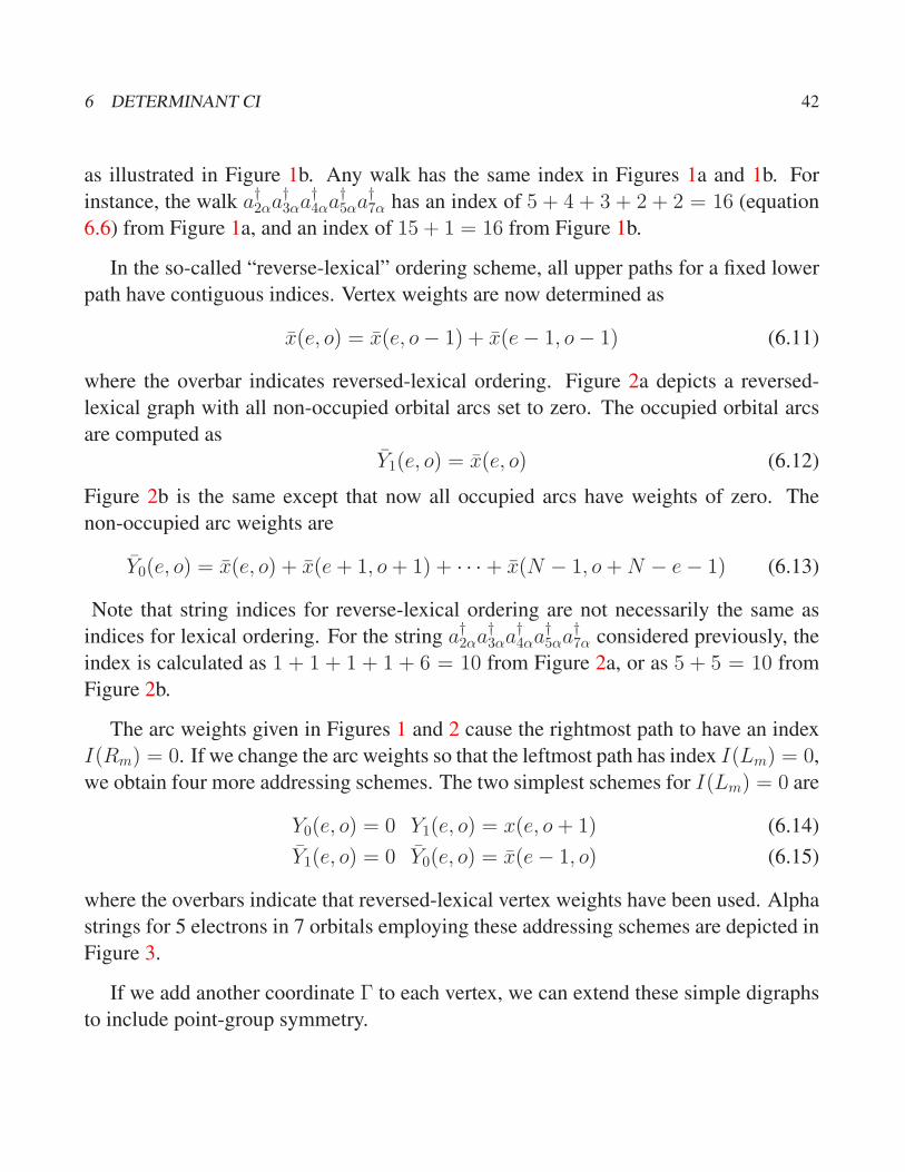
Figure 1: Alpha string graph for nα = 5, n = 7. Vertex weights are determined according to lexical
ordering, and arc weights are given so that the rightmost path has index zero. (a) All unoccupied arc
weights Y0(e, o) are zero. (b) All occupied arc weights Y1(e, o) are zero.
1
11
121
31
1
1
4
5
6
21
15
10
6
3
15
5 10
4 6
3 3
2 1
1 0
0
e0 1 2 3 4 5
1
11
121
31
1
1
4
5
6
0
0
0
0
0
5
4
3
2
1
6
5
4
3
2
21
15
10
6
3
(a)
0 1 2 3 4 5
(b)
0
1
2
3
4
5
6
7
0
1
2
3
4
5
6
7
o o
e
6 DETERMINANT CI 42
as illustrated in Figure 1b. Any walk has the same index in Figures 1a and 1b. For
instance, the walk a†2αa†3αa
†4αa
†5αa
†7α has an index of 5 + 4 + 3 + 2 + 2 = 16 (equation
6.6) from Figure 1a, and an index of 15 + 1 = 16 from Figure 1b.
In the so-called “reverse-lexical” ordering scheme, all upper paths for a fixed lower
path have contiguous indices. Vertex weights are now determined as
x(e, o) = x(e, o− 1) + x(e− 1, o− 1) (6.11)
where the overbar indicates reversed-lexical ordering. Figure 2a depicts a reversed-
lexical graph with all non-occupied orbital arcs set to zero. The occupied orbital arcs
are computed as
Y1(e, o) = x(e, o) (6.12)
Figure 2b is the same except that now all occupied arcs have weights of zero. The
non-occupied arc weights are
Y0(e, o) = x(e, o) + x(e+ 1, o+ 1) + · · ·+ x(N − 1, o+N − e− 1) (6.13)
Note that string indices for reverse-lexical ordering are not necessarily the same as
indices for lexical ordering. For the string a†2αa†3αa
†4αa
†5αa
†7α considered previously, the
index is calculated as 1 + 1 + 1 + 1 + 6 = 10 from Figure 2a, or as 5 + 5 = 10 from
Figure 2b.
The arc weights given in Figures 1 and 2 cause the rightmost path to have an index
I(Rm) = 0. If we change the arc weights so that the leftmost path has index I(Lm) = 0,
we obtain four more addressing schemes. The two simplest schemes for I(Lm) = 0 are
Y0(e, o) = 0 Y1(e, o) = x(e, o+ 1) (6.14)
Y1(e, o) = 0 Y0(e, o) = x(e− 1, o) (6.15)
where the overbars indicate that reversed-lexical vertex weights have been used. Alpha
strings for 5 electrons in 7 orbitals employing these addressing schemes are depicted in
Figure 3.
If we add another coordinate Γ to each vertex, we can extend these simple digraphs
to include point-group symmetry.

6 DETERMINANT CI 43
Figure 2: Alpha string graph for nα = 5, n = 7. Vertex weights are determined according to reverse-
lexical ordering, and arc weights are given so that the rightmost path has index zero. (a) All unoccupied
arc weights Y0(e, o) are zero. (b) Occupied arc weights Y1(e, o) are set to zero.
0 1 2 3 4 5
0
1
2
3
4
5
6
7
o
e0 1 2 3 4 5
0
1
2
3
4
5
6
7
o
e
1
(b)
1
1
1
1
1
0
0
0
0
0
1
4
1
1
2
3 3
6 4
10 5
15 6
21
1
2 1
3 1
1
5
6
1
1
1
1
1
1
1
1
2
3 3
6 4
10 5
15 6
21
15
5
4
14 3
12 2
9 1
5 0
0
(a)

6 DETERMINANT CI 44
Figure 3: Alpha string graph for nα = 5, n = 7, with arc weights determined so that the leftmost
path has index zero. (a) Vertex weights for lexical ordering, and arc weights according to Y0(e, o) =0, Y1(e, o) = x(e, o + 1). (b) Vertex weights according to reverse-lexical ordering, and arc weights
according to Y1(e, o) = 0, Y0(e, o) = x(e− 1, o).
0 1 2 3 4 5
0
1
2
3
4
5
6
7
o
e0 1 2 3 4 5
0
1
2
3
4
5
6
7
o
e
1
(b)
1
1
1
1
21
6 15
1 5 10
41
1
6
3
1
3
2
1
1
1
1
6
0
5
0
0
0
0
4
3
2
1
1
1
1
1
1
1
1
2
3 3
6 4
10 5
15 6
21
1
3
0
0
1 2
6 4
10 5
15
(a)

6 DETERMINANT CI 45
6.3 Restricted Active Space CI
The Restricted Active Space (RAS) CI method was introduced by Olsen, Roos, Jørgensen,
and Aa. Jensen [17] in 1988. The RAS method calls for the partitioning of the one-
electron basis into four subsets. The first subset consists of the core orbitals, which
are constrained to remain doubly-occupied. The remaining three subsets are labelled I,
II, and III, and the CI space is limited by requiring a minimum of p electrons in RAS
I and a maximum of q electrons in RAS III. There are no restrictions on the number of
electrons in RAS II, and thus it is analogous to the complete active space (CAS). The
full CI can be obtained as the maximum limit of the RAS space. Interestingly, although
the main focus of the paper is on the utility of the RAS method in limiting the size
of CI calculations, the maximum impact of this paper has been on the development of
determinant-based full CI algorithms [20, 21].
The RAS CI method relies on Handy’s separation of determinants into alpha and
beta strings (see section 6.2). As in other determinant-based CI methods, the basis
determinants are restricted to those having a given value of Ms. Since the number of
electrons N is also fixed, this means that the alpha and beta strings always have constant
lengths of nα and nβ, respectively. For a full CI, one forms all possible alpha and beta
strings for a given nα and nβ, and the basis determinants are all possible combinations
of these alpha and beta strings. In a RAS CI, the CI space is restricted in two ways:
first, not all alpha and beta strings are allowed, and secondly, not all combinations of
alpha and beta strings to form determinants are accepted. This is best seen from an
example: consider the case of 6 orbitals, with nα = nβ = 3. If orbitals 4, 5, and 6
constitute RAS III, with a maximum of 2 electrons allowed, then clearly alpha strings
such as a†4αa†5αa
†6α are not allowed. Similarly, even though a†1αa
†4αa
†5α and a†1βa
†4βa
†5β
are allowed alpha and beta strings, these strings cannot be combined with each other
because the resulting determinant would represent a quadruple excition into RAS III.
If we employ a graphical description of the alpha and beta strings as described in
section 6.2.1, in general we require one graph for alpha strings and one graph for beta
strings. However, in the case that Ms = 0, only one graph is needed because the alpha
string and beta string graphs are identical. As previously mentioned, for a RAS space

6 DETERMINANT CI 46
not all alpha and beta strings can be freely combined. While it would be possible to
create a table listing all allowed combinations of alpha and beta strings, there is a more
efficient way around this difficulty. Instead of using a single graph to represent all
alpha (or beta) strings, instead we use several graphs. For example, we might use one
graph for all strings with no electrons in RAS III, one graph for all strings with one
electron in RAS III, and one graph for all strings with two electrons in RAS III. In this
case, the restrictions on combinations of strings become restrictions on combinations
of graphs—a more efficient treatment computationally. Figure 4 displays string graphs
for nα = nβ = 3 and n = 6 for at most 2 electrons in RAS III, orbitals 4-6. Graph (a)
represents all walks with two electrons in RAS III; graph (b) gives all walks with one
electron in RAS III; and graph (c) gives the one walk with no electrons in RAS III. If
only two electrons are allowed in RAS III, it is clear that alpha strings of graph a can be
combined only with the beta string from graph (c), and alpha strings of graph (b) can
be combined with beta strings of graphs (b) and (c). An alpha string from graph (c) can
be combined with beta strings from graphs (a), (b), and (c).
6.3.1 Olsen’s Full CI σ Equations
We now turn our attention to the general formulation of the full CI problem in terms
of alpha and beta strings. Later on, we will consider how to modify our results for
RAS CI’s. We begin by describing Olsen’s expressions for σ, which is the action of the
Hamiltonian H on the CI vector (or matrix) C(Iα, Iβ). First we express H in second-
quantized form (see section 5).
H =n∑
kl
hklEkl +1
2
n∑
ijkl
(ij|kl)(
EijEkl − δjkEil
)
(6.16)
where Ekl is the shift operator
Ekl = Eαkl + Eβ
kl (6.17)
Again, σ is given by
σ(Iα, Iβ) =∑
Jα,Jβ
〈β(Jβ)α(Jα)|H|α(Iα)β(Iβ)〉C(Jα, Jβ) (6.18)

6 DETERMINANT CI 47
Figure 4: String graphs for nα/β = 3, n = 6 with at most two electrons in RAS III of orbitals 4-6. Vertex
weights and arc weights are given for lexical ordering.
e0 1 2 3
0
0
1
1
1
1
2
3
1
1
(b)
0
333
66
3
9
e0 1 2 3
0
0
0
1
3
1
1
1
(c)
1
1
1
0 1 2 3
1
00
1
2
3
4
5
6
(a)
e
o
1
11
2
3
1
2
0
033
6 3
9
3

6 DETERMINANT CI 48
As we will proceed to show, σ can be split up into three terms: one involving only beta
components of the linear group generators (σ1), one involving only alpha components
of the generators (σ2), and one involving mixtures of the two (σ3). Inserting equation
(6.16) into equation (6.18) yields
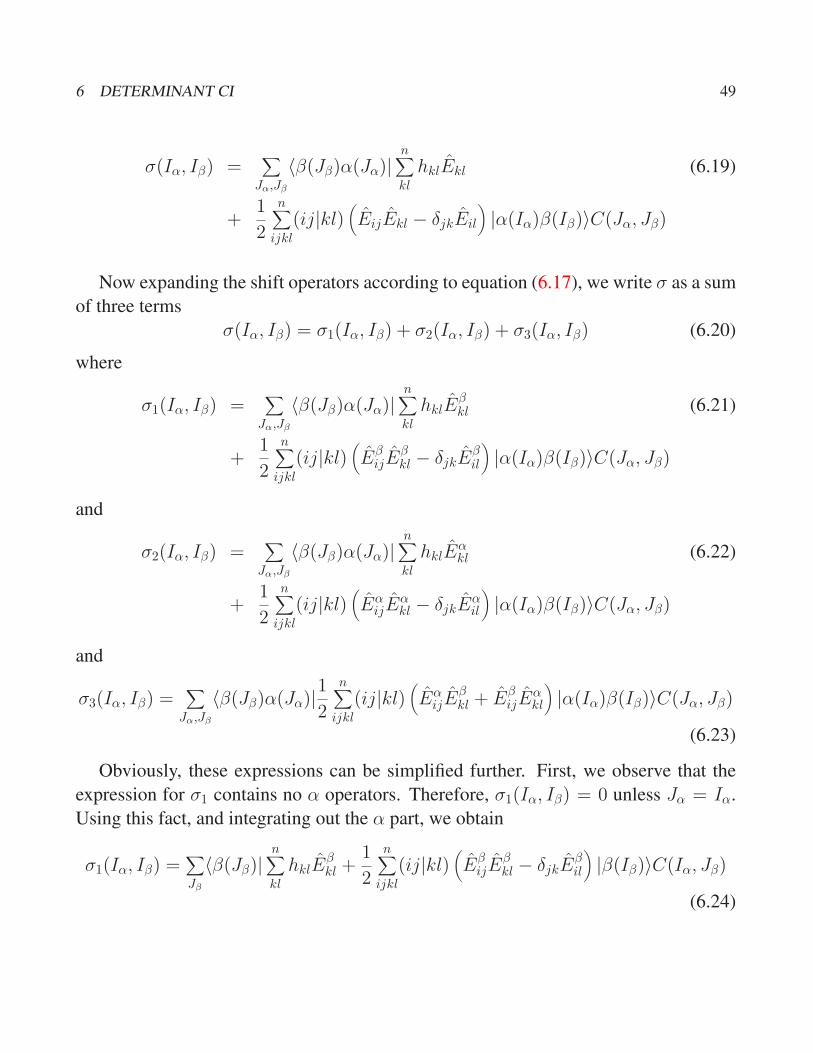
6 DETERMINANT CI 49
σ(Iα, Iβ) =∑
Jα,Jβ
〈β(Jβ)α(Jα)|n∑
kl
hklEkl (6.19)
+1
2
n∑
ijkl
(ij|kl)(
EijEkl − δjkEil
)
|α(Iα)β(Iβ)〉C(Jα, Jβ)
Now expanding the shift operators according to equation (6.17), we write σ as a sum
of three terms
σ(Iα, Iβ) = σ1(Iα, Iβ) + σ2(Iα, Iβ) + σ3(Iα, Iβ) (6.20)
where
σ1(Iα, Iβ) =∑
Jα,Jβ
〈β(Jβ)α(Jα)|n∑
kl
hklEβkl (6.21)
+1
2
n∑
ijkl
(ij|kl)(
EβijE
βkl − δjkE
βil
)
|α(Iα)β(Iβ)〉C(Jα, Jβ)
and
σ2(Iα, Iβ) =∑
Jα,Jβ
〈β(Jβ)α(Jα)|n∑
kl
hklEαkl (6.22)
+1
2
n∑
ijkl
(ij|kl)(
EαijE
αkl − δjkE
αil
)
|α(Iα)β(Iβ)〉C(Jα, Jβ)
and
σ3(Iα, Iβ) =∑
Jα,Jβ
〈β(Jβ)α(Jα)|1
2
n∑
ijkl
(ij|kl)(
EαijE
βkl + Eβ
ijEαkl
)
|α(Iα)β(Iβ)〉C(Jα, Jβ)
(6.23)
Obviously, these expressions can be simplified further. First, we observe that the
expression for σ1 contains no α operators. Therefore, σ1(Iα, Iβ) = 0 unless Jα = Iα.
Using this fact, and integrating out the α part, we obtain
σ1(Iα, Iβ) =∑
Jβ
〈β(Jβ)|n∑
kl
hklEβkl +
1
2
n∑
ijkl
(ij|kl)(
EβijE
βkl − δjkE
βil
)
|β(Iβ)〉C(Iα, Jβ)
(6.24)
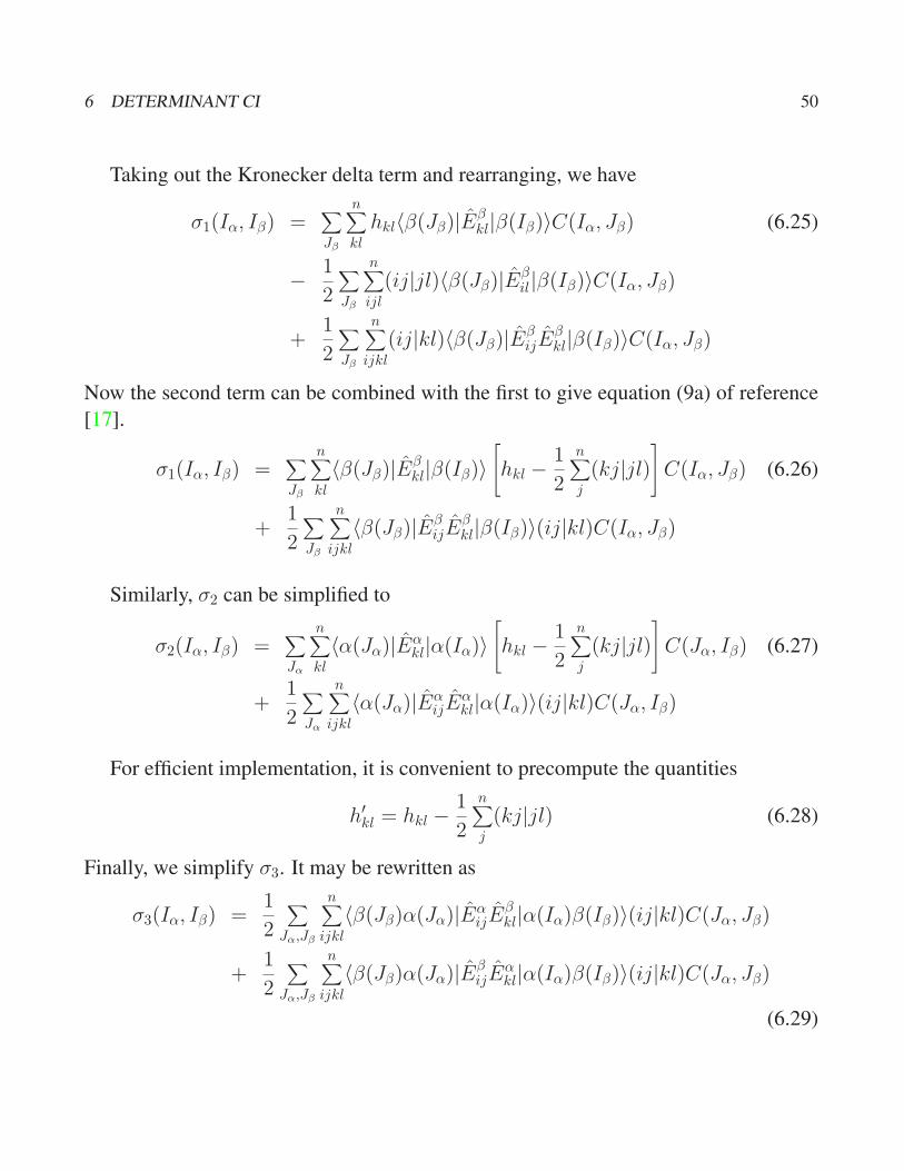
6 DETERMINANT CI 50
Taking out the Kronecker delta term and rearranging, we have
σ1(Iα, Iβ) =∑
Jβ
n∑
kl
hkl〈β(Jβ)|Eβkl|β(Iβ)〉C(Iα, Jβ) (6.25)
− 1
2
∑
Jβ
n∑
ijl
(ij|jl)〈β(Jβ)|Eβil|β(Iβ)〉C(Iα, Jβ)
+1
2
∑
Jβ
n∑
ijkl
(ij|kl)〈β(Jβ)|EβijE
βkl|β(Iβ)〉C(Iα, Jβ)
Now the second term can be combined with the first to give equation (9a) of reference
[17].
σ1(Iα, Iβ) =∑
Jβ
n∑
kl
〈β(Jβ)|Eβkl|β(Iβ)〉
hkl −1
2
n∑
j
(kj|jl)
C(Iα, Jβ) (6.26)
+1
2
∑
Jβ
n∑
ijkl
〈β(Jβ)|EβijE
βkl|β(Iβ)〉(ij|kl)C(Iα, Jβ)
Similarly, σ2 can be simplified to
σ2(Iα, Iβ) =∑
Jα
n∑
kl
〈α(Jα)|Eαkl|α(Iα)〉
hkl −1
2
n∑
j
(kj|jl)
C(Jα, Iβ) (6.27)
+1
2
∑
Jα
n∑
ijkl
〈α(Jα)|EαijE
αkl|α(Iα)〉(ij|kl)C(Jα, Iβ)
For efficient implementation, it is convenient to precompute the quantities
h′kl = hkl −
1
2
n∑
j
(kj|jl) (6.28)
Finally, we simplify σ3. It may be rewritten as
σ3(Iα, Iβ) =1
2
∑
Jα,Jβ
n∑
ijkl
〈β(Jβ)α(Jα)|EαijE
βkl|α(Iα)β(Iβ)〉(ij|kl)C(Jα, Jβ)
+1
2
∑
Jα,Jβ
n∑
ijkl
〈β(Jβ)α(Jα)|EβijE
αkl|α(Iα)β(Iβ)〉(ij|kl)C(Jα, Jβ)
(6.29)

6 DETERMINANT CI 51
Since we sum over all ijkl, we can permute i and j with k and l. We can also swap Eαij
and Eβkl as can easily be verified. This yields equation (9c) from reference [17].
σ3(Iα, Iβ) =∑
Jα,Jβ
n∑
ijkl
〈β(Jβ)|Eβij|β(Iβ)〉〈α(Jα)|Eα
kl|α(Iα)〉(ij|kl)C(Jα, Jβ)
(6.30)
Thus we have written the action of the Hamiltonian on the current CI vector in terms
of alpha and beta strings and alpha and beta shift operators. The product σ is written
as a sum of three terms: the first (σ1) involves only beta shift operators, the second
(σ2) involves only alpha shift operators, and the third (σ3) involves both alpha and beta
shift operators. Note that, except for the factor C(Iα, Jβ), σ1 is independent of Iα so
that the algorithm for computing σ1 is vectorizable (see below). Analogous results hold
for σ2. This situation does not obtain in the computation of σ3, however, which is the
rate-limiting step.
6.4 Full CI Algorithm
It is easy to vectorize the formation of σ1 since each element σ1(Iα, Iβ) can be written
as independent of Iα apart from multiplication by a factor C(Iα, Jβ). The vectorized
algorithm for the evaluation of σ1, adapted from reference [17], appears in Figure 5.
An analogous algorithm can be used to obtain σ2. However, we can also obtain σ2 for
Ms = 0 states by
σ2(Iα, Iβ) = (−1)Sσ1(Iβ, Iα) (6.31)
as proven by Olsen and co-workers [17].
A fairly straightforward algorithm for evaluating σ3 is presented in Figure 6. The
vectorized algorithm for the evaluation of σ3 is presented in Figure 7. This algorithm
makes use of a gather and scatter operation to avoid indirect addressing.
For Ms = 0, an improvement to the σ3 algorithm can be made by utilizing an
identity similar to equation (6.31). The ijklth component of σ3 is related to the klijth

6 DETERMINANT CI 52
Figure 5: Vectorized Algorithm for σ1.
loop over IβSet array F (Jβ) = 0
Loop over excitations Eβkl from |β(Iβ)〉
|β(Kβ)〉 = sgn(kl)Eβkl|β(Iβ)〉
F (Kβ)+ = sgn(kl)h′
kl
Loop over excitations Eβij from |β(Kβ)〉
|β(Jβ)〉 = sgn(ij)Eβij|β(Kβ)〉
F (Jβ)+ = (1/2)sgn(kl)sgn(ij)(ij|kl)end loop over Eβ
ij
end loop over Eβkl
σ1(Iα, Iβ) =∑
Jβ F (Jβ)C(Iα, Jβ); vect’d over Iαend loop over Iβ
Figure 6: Simple Algorithm for σ3.
loop over Iαloop over |α(Jα)〉 = sgn(kl)Eα
kl|α(Iα)〉loop over Iβ
loop over |β(Jβ)〉 = sgn(ij)Eβij|β(Iβ)〉
σ3(Iα, Iβ)+ = sgn(ij)sgn(kl)(ij|kl)C(Jα, Jβ)

6 DETERMINANT CI 53
Figure 7: Vectorized Algorithm for σ3.
loop over klset up L(I), R(I), and sgn(I), defined by
|α[L(I)]〉 = Eαkl|α[R(I)]〉sgn(I)
C ′(I, Jβ) = C[L(I), Jβ]sgn(I); vectorized gather
loop over Iβloop over excitations Eβ
ij from |β(Iβ)〉|β(Jβ)〉 = sgn(ij)Eβ
ij|β(Iβ)〉F (Jβ)+ = sgn(ij)(ij|kl)
end loop over Eβij
V (I) =∑
Jβ F (Jβ)C′(I, Jβ); vect’d over I
σ3[R(I), Iβ]+ = V (I); vectorized scatter
end loop over Iβend loop over kl
component via
σijkl3 (Iα, Iβ) = (−1)Sσklij
1 (Iβ, Iα) (6.32)

REFERENCES 54
References
[1] A. Szabo and N. S. Ostlund, Modern Quantum Chemistry: Introduction to Ad-
vanced Electronic Structure Theory. McGraw-Hill, New York, 1989.
[2] W. Heisenberg, Z. Phys. 33, 879 (1925).
[3] E. Schrodinger, Ann. d. Phys. 79, 734 (1926).
[4] C. Eckart, Phys. Rev. 28, 711 (1926).
[5] J. Paldus, J. Chem. Phys. 61, 5321 (1974).
[6] R. J. Harrison and N. C. Handy, Chem. Phys. Lett. 95, 386 (1983).
[7] I. Shavitt, The method of configuration interaction, in Methods of Electronic
Structure Theory, edited by H. F. Schaefer, pages 189–275. Plenum Press, New
York, 1977.
[8] P. E. M. Siegbahn, The direct CI method, in Methods in Computational Molecular
Physics, edited by G. H. F. Diercksen and S. Wilson, pages 189–207. D. Reidel,
Dordrecht, 1983.
[9] J. C. Slater, Phys. Rev. 34, 1293 (1929).
[10] E. U. Condon, Phys. Rev. 36, 1121 (1930).
[11] J. C. Slater, Phys. Rev. 38, 1109 (1931).
[12] W. Ritz, J. Reine Angew. Math. 135, 1 (1909).
[13] R. J. Bartlett, C. E. Dykstra, and J. Paldus, Coupled-cluster methods for molecular
calculations, in Advanced Theories and Computational Approaches to the Elec-
tronic Structure of Molecules, edited by C. E. Dykstra, pages 127–159. D. Reidel,
Dordrecht, 1984.
[14] L. Pauling and E. B. Wilson, Jr., Introduction to Quantum Mechanics with Appli-
cations to Chemistry. McGraw-Hill, New York, 1935.

REFERENCES 55
[15] J. K. L. MacDonald, Phys. Rev. 43, 830 (1933).
[16] E. A. Hylleraas and B. Undheim, Z. Phys. 65, 759 (1930).
[17] J. Olsen, B. O. Roos, P. Jørgensen, and H. J. Aa. Jensen, J. Chem. Phys. 89, 2185
(1988).
[18] J. T. Fermann, C. D. Sherrill, T. D. Crawford, and H. F. Schaefer, J. Chem. Phys.
100, 8132 (1994).
[19] P. J. Knowles and N. C. Handy, J. Chem. Phys. 91, 2396 (1989).
[20] J. Olsen, P. Jørgensen, and J. Simons, Chem. Phys. Lett. 169, 463 (1990).
[21] A. O. Mitrushenkov, Chem. Phys. Lett. 217, 559 (1994).
[22] R. P. Hosteny, T. H. Dunning, R. R. Gilman, A. Pipano, and I. Shavitt, J. Chem.
Phys. 62, 4764 (1975).
[23] V. R. Saunders and J. H. van Lenthe, Mol. Phys. 48, 923 (1983).
[24] E. R. Davidson, Perspectives on ab initio calculations, in Reviews in Computa-
tional Chemistry, edited by K. B. Lipkowitz and D. B. Boyd. VCH Publishers,
New York, 1990.
[25] W. Duch and G. H. F. Diercksen, J. Chem. Phys. 101, 3018 (1994).
[26] S. R. Langhoff and E. R. Davidson, Int. J. Quantum Chem. 8, 61 (1974).
[27] A. Povill, R. Caballol, J. Rubio, and J. P. Malrieu, Chem. Phys. Lett. 209, 126
(1993).
[28] W. Duch, GRMS or Graphical Representation of Model Spaces, volume 1.
Springer-Verlag, Berlin, 1986.
[29] G. E. Scuseria, C. L. Janssen, and H. F. Schaefer, J. Chem. Phys. 89, 7382 (1988).
[30] N. C. Handy, Chem. Phys. Lett. 74, 280 (1980).
![University of Groningen Conserving approximations in ...In quantum chemistry there are advanced wavefunction methods like configuration interaction and coupled cluster the-ory [1]](https://img.dokumen.tips/doc/110x75/5f4aca2b21acef7e0c72d2cb/university-of-groningen-conserving-approximations-in-in-quantum-chemistry-there.jpg)