Embed Size (px)
Citation preview

An Introduction to
Chemical Kinetics
An Introduction to Chemical Kinetics. Margaret Robson Wright# 2004 John Wiley & Sons, Ltd. ISBNs: 0-470-09058-8 (hbk) 0-470-09059-6 (pbk)
An Introduction to
Chemical Kinetics
Margaret Robson Wright
Formerly of The University of St Andrews, UK
Copyright # 2004 John Wiley & Sons Ltd, The Atrium, Southern Gate, Chichester,West Sussex PO19 8SQ, England
Telephone (+44) 1243 779777
Email (for orders and customer service enquiries): [email protected] our Home Page on www.wileyeurope.com or www.wiley.com
All Rights Reserved. No part of this publication may be reproduced, stored in a retrieval system or transmittedin any form or by any means, electronic, mechanical, photocopying, recording, scanning or otherwise, exceptunder the terms of the Copyright, Designs and Patents Act 1988 or under the terms of a licence issued by theCopyright Licensing Agency Ltd, 90 Tottenham Court Road, London W1T 4LP, UK, without the permissionin writing of the Publisher. Requests to the Publisher should be addressed to the Permissions Department,John Wiley & Sons Ltd, The Atrium, Southern Gate, Chichester, West Sussex PO19 8SQ, England, oremailed to [email protected], or faxed to (+44) 1243 770620.
This publication is designed to provide accurate and authoritative information in regard to the subject mattercovered. It is sold on the understanding that the Publisher is not engaged in rendering professional services. Ifprofessional advice or other expert assistance is required, the services of a competent professional should besought.
Other Wiley Editorial Offices
John Wiley & Sons Inc., 111 River Street, Hoboken, NJ 07030, USA
Jossey-Bass, 989 Market Street, San Francisco, CA 94103-1741, USA
Wiley–VCH Verlag GmbH, Boschstrasse 12, D-69469 Weinheim, Germany
John Wiley & Sons Australia Ltd, 33 Park Road, Milton, Queensland 4064, Australia
John Wiley & Sons (Asia) Pte Ltd, 2 Clementi Loop # 02-01, Jin Xing Distripark, Singapore 129809
John Wiley & Sons Canada Ltd, 22 Worcester Road, Etobicoke, Ontario, Canada M9W 1L1
Wiley also publishes its books in a variety of electronic formats. Some content that appears inprint may not be available in electronic books.
Library of Congress Cataloging-in-Publication Data
Wright, Margaret Robson.An introduction to chemical kinetics / Margaret Robson Wright.
p. cm.Includes bibliographical references and index.ISBN 0-470-09058-8 (acid-free paper) – ISBN 0-470-09059-6 (pbk. : acid-free paper)1. Chemical kinetics. I. Title.
QD502.W75 20045410.394–dc22 2004006062
British Library Cataloguing in Publication Data
A catalogue record for this book is available from the British Library
ISBN 0 470 09058 8 hardback0 470 09059 6 paperback
Typeset in 10.5/13pt Times by Thomson Press (India) Limited, New DelhiPrinted and bound in Great Britain by TJ International Ltd., Padstow, CornwallThis book is printed on acid-free paper responsibly manufactured from sustainable forestryin which at least two trees are planted for each one used for paper production.

Dedicated with much love and affection
to
my mother, Anne (in memoriam),
with deep gratitude for all her loving help,
to
her oldest and dearest friends,
Nessie (in memoriam) and Dodo Gilchrist of Cumnock, who,
by their love and faith in me, have always been a source of great
encouragement to me,
and last, but not least, to my own immediate family,
my husband, Patrick,
our children Anne, Edward and Andrew and our cats.
Contents
Preface xiii
List of Symbols xvii
1 Introduction 1
2 Experimental Procedures 52.1 Detection, Identification and Estimation of Concentration of Species Present 6
2.1.1 Chromatographic techniques: liquid–liquid and gas–liquid chromatography 6
2.1.2 Mass spectrometry (MS) 6
2.1.3 Spectroscopic techniques 7
2.1.4 Lasers 13
2.1.5 Fluorescence 14
2.1.6 Spin resonance methods: nuclear magnetic resonance (NMR) 15
2.1.7 Spin resonance methods: electron spin resonance (ESR) 15
2.1.8 Photoelectron spectroscopy and X-ray photoelectron spectroscopy 15
2.2 Measuring the Rate of a Reaction 17
2.2.1 Classification of reaction rates 17
2.2.2 Factors affecting the rate of reaction 18
2.2.3 Common experimental features for all reactions 19
2.2.4 Methods of initiation 19
2.3 Conventional Methods of Following a Reaction 20
2.3.1 Chemical methods 20
2.3.2 Physical methods 21
2.4 Fast Reactions 27
2.4.1 Continuous flow 27
2.4.2 Stopped flow 28
2.4.3 Accelerated flow 29
2.4.4 Some features of flow methods 29
2.5 Relaxation Methods 30
2.5.1 Large perturbations 31
2.5.2 Flash photolysis 31
2.5.3 Laser photolysis 32
2.5.4 Pulsed radiolysis 32
2.5.5 Shock tubes 33
2.5.6 Small perturbations: temperature, pressure and electric field jumps 33
2.6 Periodic Relaxation Techniques: Ultrasonics 35
2.7 Line Broadening in NMR and ESR Spectra 38
Further Reading 38
Further Problems 39
3 The Kinetic Analysis of Experimental Data 433.1 The Experimental Data 44
3.2 Dependence of Rate on Concentration 47
3.3 Meaning of the Rate Expression 48
3.4 Units of the Rate Constant, k 49
3.5 The Significance of the Rate Constant as Opposed to the Rate 50
3.6 Determining the Order and Rate Constant from Experimental Data 52
3.7 Systematic Ways of Finding the Order and Rate Constant from Rate/
Concentration Data 53
3.7.1 A straightforward graphical method 55
3.7.2 log/log graphical procedures 55
3.7.3 A systematic numerical procedure 56
3.8 Drawbacks of the Rate/Concentration Methods of Analysis 58
3.9 Integrated Rate Expressions 58
3.9.1 Half-lives 59
3.10 First Order Reactions 62
3.10.1 The half-life for a first order reaction 63
3.10.2 An extra point about first order reactions 64
3.11 Second Order Reactions 66
3.11.1 The half-life for a second order reaction 67
3.11.2 An extra point about second order reactions 68
3.12 Zero Order Reaction 68
3.12.1 The half-life for a zero order reaction 70
3.13 Integrated Rate Expressions for Other Orders 71
3.14 Main Features of Integrated Rate Equations 71
3.15 Pseudo-order Reactions 74
3.15.1 Application of pseudo-order techniques to rate/concentration data 75
3.16 Determination of the Product Concentration at Various Times 77
3.17 Expressing the Rate in Terms of Reactants or Products for Non-simple
Stoichiometry 79
3.18 The Kinetic Analysis for Complex Reactions 79
3.18.1 Relatively simple reactions which are mathematically complex 81
3.18.2 Analysis of the simple scheme A�!k1I�!k2
P 81
3.18.3 Two conceivable situations 82
3.19 The Steady State Assumption 84
3.19.1 Using this assumption 84
3.20 General Treatment for Solving Steady States 86
3.21 Reversible Reactions 89
3.21.1 Extension to other equilibria 90
3.22 Pre-equilibria 92
3.23 Dependence of Rate on Temperature 92
Further Reading 95
Further Problems 95
4 Theories of Chemical Reactions 994.1 Collision Theory 100
4.1.1 Definition of a collision in simple collision theory 100
4.1.2 Formulation of the total collision rate 102
4.1.3 The p factor 108
4.1.4 Reaction between like molecules 110
4.2 Modified Collision Theory 110
viii CONTENTS
4.2.1 A new definition of a collision 110
4.2.2 Reactive collisions 111
4.2.3 Contour diagrams for scattering of products of a reaction 112
4.2.4 Forward scattering: the stripping or grazing mechanism 117
4.2.5 Backward scattering: the rebound mechanism 118
4.2.6 Scattering diagrams for long-lived complexes 119
4.3 Transition State Theory 122
4.3.1 Transition state theory, configuration and potential energy 122
4.3.2 Properties of the potential energy surface relevant to transition
state theory 123
4.3.3 An outline of arguments involved in the derivation of the rate equation 131
4.3.4 Use of the statistical mechanical form of transition state theory 135
4.3.5 Comparisons with collision theory and experimental data 136
4.4 Thermodynamic Formulations of Transition State Theory 140
4.4.1 Determination of thermodynamic functions for activation 142
4.4.2 Comparison of collision theory, the partition function form and the
thermodynamic form of transition state theory 142
4.4.3 Typical approximate values of contributions entering the sign
and magnitude of �S6¼� 144
4.5 Unimolecular Theory 145
4.5.1 Manipulation of experimental results 148
4.5.2 Physical significance of the constancy or otherwise of k1, k�1 and k2 151
4.5.3 Physical significance of the critical energy in unimolecular reactions 152
4.5.4 Physical significance of the rate constants k1, k�1 and k2 153
4.5.5 The simple model: that of Lindemann 153
4.5.6 Quantifying the simple model 154
4.5.7 A more complex model: that of Hinshelwood 155
4.5.8 Quantifying Hinshelwood’s theory 155
4.5.9 Critique of Hinshelwood’s theory 157
4.5.10 An even more complex model: that of Kassel 158
4.5.11 Critique of the Kassel theory 159
4.5.12 Energy transfer in the activation step 159
4.6 The Slater Theory 160
Further Reading 162
Further Problems 162
5 Potential Energy Surfaces 1655.1 The Symmetrical Potential Energy Barrier 165
5.2 The Early Barrier 167
5.3 The Late Barrier 167
5.4 Types of Elementary Reaction Studied 168
5.5 General Features of Early Potential Energy Barriers for Exothermic Reactions 170
5.6 General Features of Late Potential Energy Surfaces for Exothermic Reactions 172
5.6.1 General features of late potential energy surfaces where the
attacking atom is light 173
5.6.2 General features of late potential energy surfaces for exothermic
reactions where the attacking atom is heavy 175
5.7 Endothermic Reactions 177
5.8 Reactions with a Collision Complex and a Potential Energy Well 178
Further Reading 180
Further Problems 180
CONTENTS ix
6 Complex Reactions in the Gas Phase 1836.1 Elementary and Complex Reactions 184
6.2 Intermediates in Complex Reactions 186
6.3 Experimental Data 188
6.4 Mechanistic Analysis of Complex Non-chain Reactions 189
6.5 Kinetic Analysis of a Postulated Mechanism: Use of the Steady State Treatment 192
6.5.1 A further example where disentangling of the kinetic data is necessary 195
6.6 Kinetically Equivalent Mechanisms 198
6.7 A Comparison of Steady State Procedures and Equilibrium Conditions in
the Reversible Reaction 202
6.8 The Use of Photochemistry in Disentangling Complex Mechanisms 204
6.8.1 Kinetic features of photochemistry 204
6.8.2 The reaction of H2 with I2 206
6.9 Chain Reactions 208
6.9.1 Characteristic experimental features of chain reactions 209
6.9.2 Identification of a chain reaction 210
6.9.3 Deduction of a mechanism from experimental data 211
6.9.4 The final stage: the steady state analysis 213
6.10 Inorganic Chain Mechanisms 213
6.10.1 The H2/Br2 reaction 213
6.10.2 The steady state treatment for the H2/Br2 reaction 214
6.10.3 Reaction without inhibition 216
6.10.4 Determination of the individual rate constants 217
6.11 Steady State Treatments and Possibility of Determination of All the Rate
Constants 218
6.11.1 Important points to note 221
6.12 Stylized Mechanisms: A Typical Rice–Herzfeld Mechanism 221
6.12.1 Dominant termination steps 223
6.12.2 Relative rate constants for termination steps 224
6.12.3 Relative rates of the termination steps 224
6.12.4 Necessity for third bodies in termination 227
6.12.5 The steady state treatment for chain reactions, illustrating the use
of the long chains approximation 229
6.12.6 Further problems on steady states and the Rice–Herzfeld mechanism 233
6.13 Special Features of the Termination Reactions: Termination at the Surface 240
6.13.1 A general mechanism based on the Rice–Herzfeld mechanism
used previously 240
6.14 Explosions 243
6.14.1 Autocatalysis and autocatalytic explosions 244
6.14.2 Thermal explosions 244
6.14.3 Branched chain explosions 244
6.14.4 A highly schematic and simplified mechanism for a
branched chain reaction 246
6.14.5 Kinetic criteria for non-explosive and explosive reaction 247
6.14.6 A typical branched chain reaction showing explosion limits 249
6.14.7 The dependence of rate on pressure and temperature 250
6.15 Degenerate Branching or Cool Flames 252
6.15.1 A schematic mechanism for hydrocarbon combustion 254
6.15.2 Chemical interpretation of ‘cool’ flame behaviour 257
Further Reading 259
Further Problems 260
x CONTENTS
7 Reactions in Solution 2637.1 The Solvent and its Effect on Reactions in Solution 263
7.2 Collision Theory for Reactions in Solution 265
7.2.1 The concepts of ideality and non-ideality 268
7.3 Transition State Theory for Reactions in Solution 269
7.3.1 Effect of non-ideality: the primary salt effect 269
7.3.2 Dependence of �S6¼� and �H 6¼� on ionic strength 279
7.3.3 The effect of the solvent 280
7.3.4 Extension to include the effect of non-ideality 284
7.3.5 Deviations from predicted behaviour 284
7.4 �S6¼� and Pre-exponential A Factors 289
7.4.1 A typical problem in graphical analysis 292
7.4.2 Effect of the molecularity of the step for which �S6¼� is found 292
7.4.3 Effect of complexity of structure 292
7.4.4 Effect of charges on reactions in solution 293
7.4.5 Effect of charge and solvent on �S6¼� for ion–ion reactions 293
7.4.6 Effect of charge and solvent on �S6¼� for ion–molecule reactions 295
7.4.7 Effect of charge and solvent on �S6¼� for molecule–molecule reactions 296
7.4.8 Effects of changes in solvent on �S6¼� 296
7.4.9 Changes in solvation pattern on activation, and the effect on A factors
for reactions involving charges and charge-separated species in solution 296
7.4.10 Reactions between ions in solution 297
7.4.11 Reaction between an ion and a molecule 298
7.4.12 Reactions between uncharged polar molecules 299
7.5 �H 6¼� Values 301
7.5.1 Effect of the molecularity of the step for which the �H 6¼� value
is found 301
7.5.2 Effect of complexity of structure 302
7.5.3 Effect of charge and solvent on �H 6¼� for ion–ion and
ion–molecule reactions 302
7.5.4 Effect of the solvent on �H 6¼� for ion–ion and ion–molecule reactions 303
7.5.5 Changes in solvation pattern on activation and the effect on �H 6¼� 303
7.6 Change in Volume on Activation, �V 6¼� 304
7.6.1 Effect of the molecularity of the step for which �V 6¼� is found 305
7.6.2 Effect of complexity of structure 306
7.6.3 Effect of charge on �V 6¼� for reactions between ions 306
7.6.4 Reactions between an ion and an uncharged molecule 308
7.6.5 Effect of solvent on �V 6¼� 308
7.6.6 Effect of change of solvation pattern on activation and its
effect on �V 6¼� 308
7.7 Terms Contributing to Activation Parameters 310
7.7.1 �S6¼� 310
7.7.2 �V 6¼� 310
7.7.3 �H 6¼� 311
Further Reading 314
Further Problems 314
8 Examples of Reactions in Solution 3178.1 Reactions Where More than One Reaction Contributes to the Rate of
Removal of Reactant 317
8.1.1 A simple case 318
CONTENTS xi
8.1.2 A slightly more complex reaction where reaction occurs by two concurrent
routes, and where both reactants are in equilibrium with each other 321
8.1.3 Further disentangling of equilibria and rates, and the possibility of
kinetically equivalent mechanisms 328
8.1.4 Distinction between acid and base hydrolyses of esters 331
8.2 More Complex Kinetic Situations Involving Reactants in Equilibrium with Each
Other and Undergoing Reaction 336
8.2.1 A further look at the base hydrolysis of glycine ethyl ester as an
illustration of possible problems 336
8.2.2 Decarboxylations of �-keto-monocarboxylic acids 339
8.2.3 The decarboxylation of �-keto-dicarboxylic acids 341
8.3 Metal Ion Catalysis 344
8.4 Other Common Mechanisms 346
8.4.1 The simplest mechanism 346
8.4.2 Kinetic analysis of the simplest mechanism 347
8.4.3 A slightly more complex scheme 351
8.4.4 Standard procedure for determining the expression for kobs for
the given mechanism (Section 8.4.3) 352
8.5 Steady States in Solution Reactions 359
8.5.1 Types of reaction for which a steady state treatment could be relevant 359
8.5.2 A more detailed analysis of Worked Problem 6.5 360
8.6 Enzyme Kinetics 365
Further Reading 368
Further Problems 369
Answers to Problems 373
List of Specific Reactions 427
Index 431
xii CONTENTS
Preface
This book leads on from elementary basic kinetics, and covers the main topics which
are needed for a good working knowledge and understanding of the fundamental
aspects of kinetics. It emphasizes how experimental data is collected and manipulated
to give standard kinetic quantities such as rates, rate constants, enthalpies, entropies
and volumes of activation. It also emphasizes how these quantities are used in
interpretations of the mechanism of a reaction. The relevance of kinetic studies to
aspects of physical, inorganic, organic and biochemical chemistry is illustrated
through explicit reference and examples. Kinetics provides a unifying tool for all
branches of chemistry, and this is something which is to be encouraged in teaching
and which is emphasized here.
Gas studies are well covered with extensive explanation and interpretation of
experimental data, such as steady state calculations, all illustrated by frequent use of
worked examples. Solution kinetics are similarly explained, and plenty of practice is
given in dealing with the effects of the solvent and non-ideality. Students are given
plenty of practice, via worked problems, in handling various types of mechanism
found in solution, and in interpreting ionic strength dependences and enthalpies,
entropies and volumes of activation.
As the text is aimed at undergraduates studying core physical chemistry, only the
basics of theoretical kinetics are given, but the fundamental concepts are clearly
explained. More advanced reading is given in my book Fundamental Chemical
Kinetics (see reading lists).
Many students veer rapidly away from topics which are quantitative and involve
mathematical equations. This book attempts to allay these fears by guiding the
student through these topics in a step-by-step development which explains the logic,
reasoning and actual manipulation. For this reason a large fraction of the text is
devoted to worked examples, and each chapter ends with a collection of further
problems to which detailed and explanatory answers are given. If through the written
word I can help students to understand and to feel confident in their ability to learn,
and to teach them, in a manner which gives them the feeling of a direct contact with
the teacher, then this book will not have been written in vain. It is the teacher’s duty to
show students how to achieve understanding, and to think scientifically. The
philosophy behind this book is that this is best done by detailed explanation and
guidance. It is understanding, being able to see for oneself and confidence which help
to stimulate and sustain interest. This book attempts to do precisely that.

This book is the result of the accumulated experience of 40 very stimulating years
of teaching students at all levels. During this period I regularly lectured to students,
but more importantly I was deeply involved in devising tutorial programmes at all
levels where consolidation of lecture material was given through many problem-
solving exercises. I also learned that providing detailed explanatory answers to these
exercises proved very popular and successful with students of all abilities. During
these years I learned that being happy to help and being prepared to give extra
explanation and to spend extra time on a topic could soon clear up problems and
difficulties which many students thought they would never understand. Too often
teachers forget that there were times when they themselves could not understand, and
when a similar explanation and preparedness to give time were welcome. To all the
many students who have provided the stimulus and enjoyment of teaching I give my
grateful thanks.
I am very grateful to John Wiley & Sons for giving me the opportunity to publish
this book, and to indulge my love of teaching. In particular, I would like to thank
Andy Slade, Rachael Ballard and Robert Hambrook of John Wiley & Sons who have
cheerfully, and with great patience, guided me through the problems of preparing the
manuscript for publication. Invariably, they all have been extremely helpful.
I also extend my very grateful thanks to Martyn Berry who read the whole
manuscript and sent very encouraging, very helpful and constructive comments on
this book. His belief in the method of approach and his enthusiasm has been an
invaluable support to me.
Likewise, I would like to thank Professor Derrick Woollins of St Andrews
University for his continued very welcome support and encouragement throughout
the writing of this book.
To my mother, Mrs Anne Robson, I have a very deep sense of gratitude for all the
help she gave me in her lifetime in furthering my academic career. I owe her an
enormous debt for her invaluable, excellent and irreplaceable help with my children
when they were young and I was working part-time during the teaching terms of the
academic year. Without her help and her loving care of my children I would never
have gained the continued experience in teaching, and I could never have written this
book. My deep and most grateful thanks are due to her.
My husband, Patrick, has, throughout my teaching career and throughout the
thinking about and writing of this book, been a source of constant support and help
and encouragement. His very high intellectual calibre and wide-ranging knowledge
and understanding have provided many fruitful and interesting discussions. He has
read in detail the whole manuscript and his clarity, insight and considerable knowl-
edge of the subject matter have been of invaluable help. I owe him many apologies for
the large number of times when I have interrupted his own activities to pursue a
discussion of aspects of the material presented here. It is to his very great credit that I
have never been made to feel guilty about doing so. My debt to him is enormous, and
my most grateful thanks are due to him.
Finally, my thanks are due to my three children who have always encouraged me in
my teaching, and have encouraged me in the writing of my books. In particular, Anne
xiv PREFACE

and Edward have been around during the writing of this book and have given me
every encouragement to keep going.
Margaret Robson Wright
Formerly Universities of Dundee and St Andrews
October, 2003
PREFACE xv
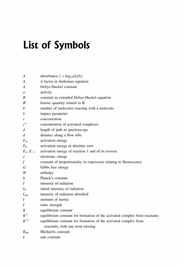
List of Symbols
A absorbance {¼ log10(I0/I)}
A A factor in Arrhenius equation
A Debye-Huckel constant
a activity
B constant in extended Debye-Huckel equation
B0 kinetic quantity related to B
b number of molecules reacting with a molecule
b impact parameter
c concentration
c 6¼ concentration of activated complexes
d length of path in spectroscopy
d distance along a flow tube
EA activation energy
E0 activation energy at absolute zero
E1, E�1 activation energy of reaction 1 and of its reverse
e electronic charge
f constant of proportionality in expression relating to fluorescence
G Gibbs free energy
H enthalpy
h Planck’s constant
I intensity of radiation
I0 initial intensity of radiation
Iabs intensity of radiation absorbed
I moment of inertia
I ionic strength
K equilibrium constant
K 6¼ equilibrium constant for formation of the activated complex from reactants
K 6¼� equilibrium constant for formation of the activated complex from
reactants, with one term missing
KM Michaelis constant
k rate constant
k1, k�1 rate constant for reaction 1 and its reverse
k Boltzmann’s constant
m mass
n order of a reaction
N 6¼ number of activated complexes
p pressure
pi partial pressure of species i
p p factor in collision theory
Q molecular partition function per unit volume
Q 6¼ molecular partition function per unit volume for the activated complex
Q 6¼ � molecular partition function per unit volume for the activated complex,
but with one term missing
R the gas constant
r internuclear distance
r 6¼ distance between the centres of ions in the activated complex
S entropy
s half of the number of squared terms, in theories of Hinshelwood
and Kassel
T absolute temperature
t time
U energy
V volume
V velocity of sound
Vs term in Michaelis-Menten equation
v velocity
v relative velocity
v vibrational quantum number
Z collision number
�Z collision rate
z number of charges
� order with respect to one reactant
� branching coefficient
� polarisability
� order with respect to one reactant
� activity coefficient
� change in
�G� standard change in free energy
�H� standard change in enthalpy
�S� standard change in entropy
�V� standard change in volume
xviii LIST OF SYMBOLS
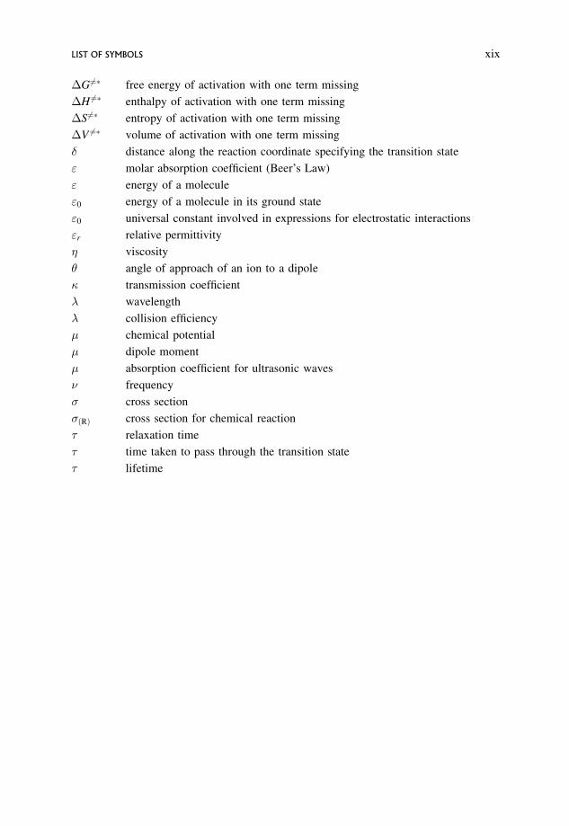
�G 6¼� free energy of activation with one term missing
�H 6¼� enthalpy of activation with one term missing
�S 6¼� entropy of activation with one term missing
�V 6¼� volume of activation with one term missing
� distance along the reaction coordinate specifying the transition state
" molar absorption coefficient (Beer’s Law)
" energy of a molecule
"0 energy of a molecule in its ground state
"0 universal constant involved in expressions for electrostatic interactions
"r relative permittivity
� viscosity
� angle of approach of an ion to a dipole
� transmission coefficient
wavelength
collision efficiency
chemical potential
dipole moment
absorption coefficient for ultrasonic waves
� frequency
� cross section
�ðRÞ cross section for chemical reaction
relaxation time
time taken to pass through the transition state
lifetime
LIST OF SYMBOLS xix
1 Introduction
Chemical kinetics is conventionally regarded as a topic in physical chemistry. In this
guise it covers the measurement of rates of reaction, and the analysis of the
experimental data to give a systematic collection of information which summarises
all the quantitative kinetic information about any given reaction. This, in turn, enables
comparisons of reactions to be made and can afford a kinetic classification of
reactions. The sort of information used here is summarized in terms of
� the factors influencing rates of reaction,
� the dependence of the rate of the reaction on concentration, called the order of the
reaction,
� the rate expression, which is an equation which summarizes the dependence of the
rate on the concentrations of substances which affect the rate of reaction,
� this expression involves the rate constant which is a constant of proportionality
linking the rate with the various concentration terms,
� this rate constant collects in one quantity all the information needed to calculate
the rate under specific conditions,
� the effect of temperature on the rate of reaction. Increase in temperature generally
increases the rate of reaction. Knowledge of just exactly how temperature affects
the rate constant can give information leading to a deeper understanding of how
reactions occur.
All of these factors are explained in Chapters 2 and 3, and problems are given to aid
understanding of the techniques used in quantifying and systematizing experimental
data.
However, the science of kinetics does not end here. The next task is to look at the
chemical steps involved in a chemical reaction, and to develop a mechanism which
summarizes this information. Chapters 6 and 8 do this for gas phase and solution
phase reactions respectively.
An Introduction to Chemical Kinetics. Margaret Robson Wright# 2004 John Wiley & Sons, Ltd. ISBNs: 0-470-09058-8 (hbk) 0-470-09059-6 (pbk)
The final task is to develop theories as to why and how reactions occur, and to
examine the physical and chemical requirements for reaction. This is a very important
aspect of modern kinetics. Descriptions of the fundamental concepts involved in the
theories which have been put forward, along with an outline of the theoretical
development, are given in Chapter 4 for gas phase reactions, and in Chapter 7 for
solution reactions.
However, kinetics is not just an aspect of physical chemistry. It is a unifying topic
covering the whole of chemistry, and many aspects of biochemistry and biology. It is
also of supreme importance in both the chemical and pharmaceutical industries. Since
the mechanism of a reaction is intimately bound up with kinetics, and since
mechanism is a major topic of inorganic, organic and biological chemistry, the
subject of kinetics provides a unifying framework for these conventional branches of
chemistry. Surface chemistry, catalysis and solid state chemistry all rest heavily on a
knowledge of kinetic techniques, analysis and interpretation. Improvements in
computers and computing techniques have resulted in dramatic advances in quantum
mechanical calculations of the potential energy surfaces of Chapters 4 and 5, and in
theoretical descriptions of rates of reaction. Kinetics also makes substantial con-
tributions to the burgeoning subject of atmospheric chemistry and environmental
studies.
Arrhenius, in the 1880s, laid the foundations of the subject as a rigorous science
when he postulated that not all molecules can react: only those which have a certain
critical minimum energy, called the activation energy, can react. There are two ways
in which molecules can acquire energy or lose energy. The first one is by absorption
of energy when radiation is shone on to the substance and by emission of energy.
Such processes are important in photochemical reactions. The second mechanism is
by energy transfer during a collision, where energy can be acquired on collision,
activation, or lost on collision, deactivation. Such processes are of fundamental
importance in theoretical kinetics where the ‘how’ and ‘why’ of reaction is
investigated. Early theoretical work using the Maxwell–Boltzmann distribution led
to collision theory. This gave an expression for the rate of reaction in terms of the rate
of collision of the reacting molecules. This collision rate is then modified to account
for the fact that only a certain fraction of the reacting molecules will react, that
fraction being the number of molecules which have energy above the critical
minimum value. As is shown in Chapter 4, collision theory affords a physical
explanation of the exponential relationship between the rate constant and the absolute
temperature.
Collision theory encouraged more experimental work and met with considerable
success for a growing number of reactions.
However, the theory appeared not to be able to account for the behaviour
of unimolecular reactions, which showed first order behaviour at high pressures,
moving to second order behaviour at low pressures. If one of the determining
features of reaction rate is the rate at which molecules collide, unimolecular reactions
might be expected always to give second order kinetics, which is not what is
observed.
2 INTRODUCTION

This problem was resolved in 1922 when Lindemann and Christiansen proposed
their hypothesis of time lags, and this mechanistic framework has been used in all the
more sophisticated unimolecular theories. It is also common to the theoretical
framework of bimolecular and termolecular reactions. The crucial argument is that
molecules which are activated and have acquired the necessary critical minimum
energy do not have to react immediately they receive this energy by collision. There
is sufficient time after the final activating collision for the molecule to lose its critical
energy by being deactivated in another collision, or to react in a unimolecular step.
It is the existence of this time lag between activation by collision and reaction
which is basic and crucial to the theory of unimolecular reactions, and this
assumption leads inevitably to first order kinetics at high pressures, and second
order kinetics at low pressures.
Other elementary reactions can be handled in the same fundamental way:
molecules can become activated by collision and then last long enough for there to
be the same two fates open to them. The only difference lies in the molecularity of the
actual reaction step:
� in a unimolecular reaction, only one molecule is involved at the actual moment of
chemical transformation;
� in a bimolecular reaction, two molecules are involved in this step;
� in a termolecular reaction, three molecules are now involved.
Aþ A �!k1 A� þ A bimolecular activation by collision
A� þ A �!k�1 Aþ A bimolecular deactivation by collision
A� þ bA �!k2 products reaction step
where A� is an activated molecule with enough energy to react.
b ¼ 0 defines spontaneous breakdown of A�,
b ¼ 1 defines bimolecular reaction involving the coming together of A� with A
and
b ¼ 2 defines termolecular reaction involving the coming together of A� with two
As.
This is a mechanism common to all chemical reactions since it describes each
individual reaction step in a complex reaction where there are many steps.
Meanwhile, in the 1930s, the idea of reaction being defined in terms of the spatial
arrangements of all the atoms in the reacting system crystallized into transition state
theory. This theory has proved to be of fundamental importance. Reaction is now
defined as the acquisition of a certain critical geometrical configuration of all the
atoms involved in the reaction, and this critical configuration was shown to have a
critical maximum in potential energy with respect to reactants and products.
INTRODUCTION 3
The lowest potential energy pathway between the reactant and product configura-
tions represents the changes which take place during reaction, and is called the
reaction coordinate or minimum energy path. The critical configuration lies on this
pathway at the configuration with the highest potential energy. It is called the
transition state or activated complex, and it must be attained before reaction can
take place. The rate of reaction is the rate at which the reactants pass through this
critical configuration. Transition state theory thus deals with the third step in the
master mechanism above. It does not discuss the energy transfers of the first two steps
of activation and deactivation.
Transition state theory, especially with its recent developments, has proved a very
powerful tool, vastly superior to collision theory. It has only recently been challenged
by modern advances in molecular beams and molecular dynamics which look at the
microscopic details of a collision, and which can be regarded as a modified collision
theory. These developments along with computer techniques, and modern experi-
mental advances in spectroscopy and lasers along with fast reaction techniques, are
now revolutionizing the science of reaction rates.
4 INTRODUCTION
2 Experimental Procedures
The five main components of any kinetic investigation are
1. product and intermediate detection,
2. concentration determination of all species present,
3. deciding on a method of following the rate,
4. the kinetic analysis and
5. determination of the mechanism.
Aims
This chapter will examine points 1--3 listed above. By the end of this chapter youshould be able to
� decide on a method for detecting and estimating species present in a reactionmixture,
� distinguish between fast reactions and the rest,
� explain the basis of conventional methods of following reactions,
� convert experimental observations into values of [reactant] remaining at giventimes,
� describe methods for following fast reactions and
� list the essential features of each method used for fast reactions.
An Introduction to Chemical Kinetics. Margaret Robson Wright# 2004 John Wiley & Sons, Ltd. ISBNs: 0-470-09058-8 (hbk) 0-470-09059-6 (pbk)
2.1 Detection, Identification and Estimation of
Concentration of Species Present
Modern work generally uses three major techniques, chromatography, mass spectro-
metry and spectroscopy, although there is a wide range of other techniques available.
2.1.1 Chromatographic techniques: liquid–liquid and
gas–liquid chromatography (GLC)
When introduced, chromatographic techniques completely revolutionized analysis of
reaction mixtures and have proved particularly important for kinetic studies of
complex gaseous reactions. A complete revision of most gas phase reactions proved
necessary, because it was soon discovered that many intermediates and minor
products had not been detected previously, and a complete re-evaluation of gas
phase mechanisms was essential.
Chromatography refers to the separation of the components in a sample by
distribution of these components between two phases, one of which is stationary
and one of which moves. This takes place in a column, and once the components have
come off the column, identification then takes place in a detector.
The main virtues of chromatographic techniques are versatility, accuracy, speed of
analysis and the ability to handle complex mixtures and separate the components
accurately. Only very small samples are required, and the technique can detect and
measure very small amounts e.g. 10�10 mol or less. Analysis times are of the order of
a few seconds for liquid samples, and even shorter for gases. However, a lower
limit around 10�3 s makes the technique unsuitable for species of shorter lifetime
than this.
Chromatography is often linked to a spectroscopic technique for liquid mixtures
and to a mass spectrometer for gaseous mixtures. Chromatography separates the
components; the other technique identifies them and determines concentrations.
2.1.2 Mass spectrometry (MS)
In mass spectrometry the sample is vaporized, and bombarded with electrons so that
the molecules are ionized. The detector measures the mass/charge ratio, from which
the molecular weight is determined and the molecule identified. Radicals often
give the same fragment ions as the parent molecules, but they can be distinguished
because lower energies are needed for the radical.
Most substances can be detected provided they can be vaporized. Only very small
samples are required, with as little as 10�12 mol being detected. Samples are leaked
directly from the reaction mixture; the time of analysis is short, around 10�5 s, and so
6 EXPERIMENTAL PROCEDURES
fairly reactive species can be studied. For highly complex mixtures, MS is linked to
chromatography, which first separates the components.
Many reaction types can be studied in the mass spectrometer: e.g. flash photolysis,
shock tube, combustion, explosions, electric discharge and complex gas reactions.
Mass spectrometry is ideal for ion–ion and ion–molecule reactions, isotopic analysis
and kinetic isotope effect studies.
2.1.3 Spectroscopic techniques
There are three important features of spectra which are of prime interest to the
kineticist.
1. The frequency and the fine structure of the lines give the identity of the molecule;
this is particularly important in detecting intermediates and minor products.
2. The intensity of the lines gives the concentration; this is useful for monitoring the
concentrations of reactants and intermediates with time.
3. The line width enables kinetic features of the transition and the excited state to be
determined.
In spectroscopic experiments, radiation is absorbed (absorption spectra) or emitted
(emission spectra). The frequency of absorption, or emission, is a manifestation of
transitions occurring within the molecule, and the frequency of a line in the spectrum
is related to the energy change as the molecule moves from one energy state to
another.
h� ¼ "0 � "00 ¼ �" ð2:1Þ
where "0 and "00 are the energies of the upper and lower levels involved in the
transition. These states are unique to any given molecule, radical or ion, and so the
lines in a spectrum are a unique fingerprint of the molecule in question. Regions of
the electromagnetic spectrum are characteristic of types of transition occurring within
the molecule. These can be changes in rotational, vibrational, electronic and nuclear
and electronic spin states.
Identification of species present during a reaction
Microwave, infrared, Raman, visible and UV spectra are all used extensively for
identification. In the gas phase these show sharp lines so that identification is easy. In
solution, the complexity of the spectra gives them sufficient features to make them
recognizably specific to the molecule in question.
DETECTION, IDENTIFICATION AND ESTIMATION OF CONCENTRATION OF SPECIES PRESENT 7
Concentration determination
Using Beer’s law, concentrations can be found from the change in intensity of the
radiation passed through the sample. The absorbance, A, of the sample at a given
wavelength is defined as
A ¼ log10 I0=I ð2:2Þ
where I0 is the incident intensity and I the final intensity. Beer’s law relates this
absorbance to the concentration of the species being monitored:
A� ¼ "�cd ð2:3Þ
where "� is the absorption coefficient for the molecule in question.
"� depends on the wavelength and the identity of the molecule.
� is the wavelength, d is the path-length and c is the concentration of the absorbing
species.
Provided that "� and d are known, the concentration of absorbing species can be
found. A calibration graph of A versus c should be linear with slope "�d and zero
intercept. Microwave, infra-red, Raman, visible and UV spectra are all used.
Special features of absorbance measurements
If the reaction being monitored is first order, i.e. has rate / [reactant]1, or is being
studied under pseudo-first order conditions, Section 3.15, the absorbance can be used
directly, eliminating the need to know the value of "�. Chapter 3 will show that such
reactions can be quantified by plotting loge[reactant] against time. Since absorbance
/ [reactant], then loge absorbance can be plotted directly against time without the
need to convert absorbance to concentration using Beer’s law.
A ¼ "cd and so c ¼ A
"dð2:4Þ
loge c ¼ loge
A
"d¼ loge A� loge "d ð2:5Þ
Since "d is a constant in any given experiment, then loge "d is also a constant, and
loge A ¼ loge cþ constant ð2:6Þ
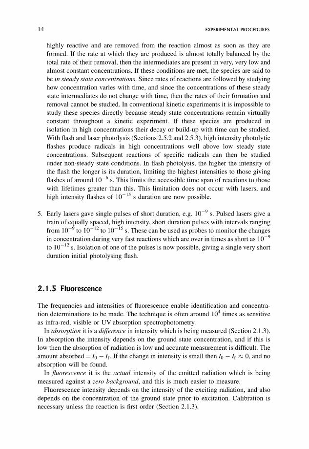
A plot of loge A versus time differs from a plot of loge c versus time only in so far as it
is displaced up the y-axis by an amount equal to loge "d (see Figure 2.1). The slope of
8 EXPERIMENTAL PROCEDURES
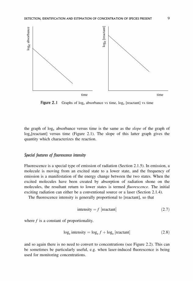
the graph of loge absorbance versus time is the same as the slope of the graph of
loge[reactant] versus time (Figure 2.1). The slope of this latter graph gives the
quantity which characterizes the reaction.
Special features of fluorescence intensity
Fluorescence is a special type of emission of radiation (Section 2.1.5). In emission, a
molecule is moving from an excited state to a lower state, and the frequency of
emission is a manifestation of the energy change between the two states. When the
excited molecules have been created by absorption of radiation shone on the
molecules, the resultant return to lower states is termed fluorescence. The initial
exciting radiation can either be a conventional source or a laser (Section 2.1.4).
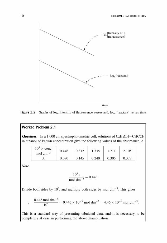
The fluorescence intensity is generally proportional to [reactant], so that
intensity ¼ f ½reactant ð2:7Þ
where f is a constant of proportionality.
loge intensity ¼ loge f þ loge ½reactant ð2:8Þ
and so again there is no need to convert to concentrations (see Figure 2.2). This can
be sometimes be particularly useful, e.g. when laser-induced fluorescence is being
used for monitoring concentrations.
time
log e
abs
orba
nce
time
log e
[re
acta
nt]
Figure 2.1 Graphs of loge absorbance vs time, loge [reactant] vs time
DETECTION, IDENTIFICATION AND ESTIMATION OF CONCENTRATION OF SPECIES PRESENT 9
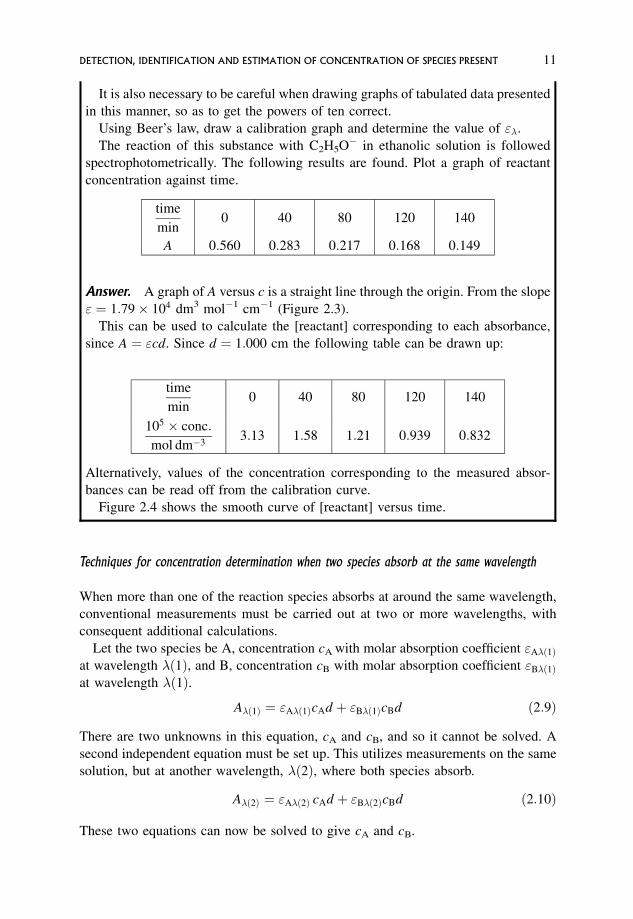
Worked Problem 2.1
Question. In a 1.000 cm spectrophotometric cell, solutions of C6H5CH����CHCCl2in ethanol of known concentration give the following values of the absorbance, A.
105 � conc:
mol dm�30:446 0:812 1:335 1:711 2:105
A 0:080 0:145 0:240 0:305 0:378
Note.
105 c
mol dm�3¼ 0:446
Divide both sides by 105, and multiply both sides by mol dm�3. This gives
c ¼ 0:446 mol dm�3
105¼ 0:446� 10�5 mol dm�3 ¼ 4:46� 10�6 mol dm�3:
This is a standard way of presenting tabulated data, and it is necessary to be
completely at ease in performing the above manipulation.
time
loge [reactant]
logeIntensity offluorescence} }
Figure 2.2 Graphs of loge intensity of fluorescence versus and, loge [reactant] versus time
10 EXPERIMENTAL PROCEDURES
It is also necessary to be careful when drawing graphs of tabulated data presented
in this manner, so as to get the powers of ten correct.
Using Beer’s law, draw a calibration graph and determine the value of "�.
The reaction of this substance with C2H5O� in ethanolic solution is followed
spectrophotometrically. The following results are found. Plot a graph of reactant
concentration against time.
time
min0 40 80 120 140
A 0:560 0:283 0:217 0:168 0:149
Answer. A graph of A versus c is a straight line through the origin. From the slope
" ¼ 1:79� 104 dm3 mol�1 cm�1 (Figure 2.3).
This can be used to calculate the [reactant] corresponding to each absorbance,
since A ¼ "cd. Since d ¼ 1:000 cm the following table can be drawn up:
time
min0 40 80 120 140
105 � conc:
mol dm�33:13 1:58 1:21 0:939 0:832
Alternatively, values of the concentration corresponding to the measured absor-
bances can be read off from the calibration curve.
Figure 2.4 shows the smooth curve of [reactant] versus time.
Techniques for concentration determination when two species absorb at the same wavelength
When more than one of the reaction species absorbs at around the same wavelength,
conventional measurements must be carried out at two or more wavelengths, with
consequent additional calculations.
Let the two species be A, concentration cA with molar absorption coefficient "A�ð1Þat wavelength �ð1Þ, and B, concentration cB with molar absorption coefficient "B�ð1Þat wavelength �ð1Þ.
A�ð1Þ ¼ "A�ð1ÞcAd þ "B�ð1ÞcBd ð2:9Þ
There are two unknowns in this equation, cA and cB, and so it cannot be solved. A
second independent equation must be set up. This utilizes measurements on the same
solution, but at another wavelength, �ð2Þ, where both species absorb.
A�ð2Þ ¼ "A�ð2Þ cAd þ "B�ð2ÞcBd ð2:10Þ
These two equations can now be solved to give cA and cB.
DETECTION, IDENTIFICATION AND ESTIMATION OF CONCENTRATION OF SPECIES PRESENT 11
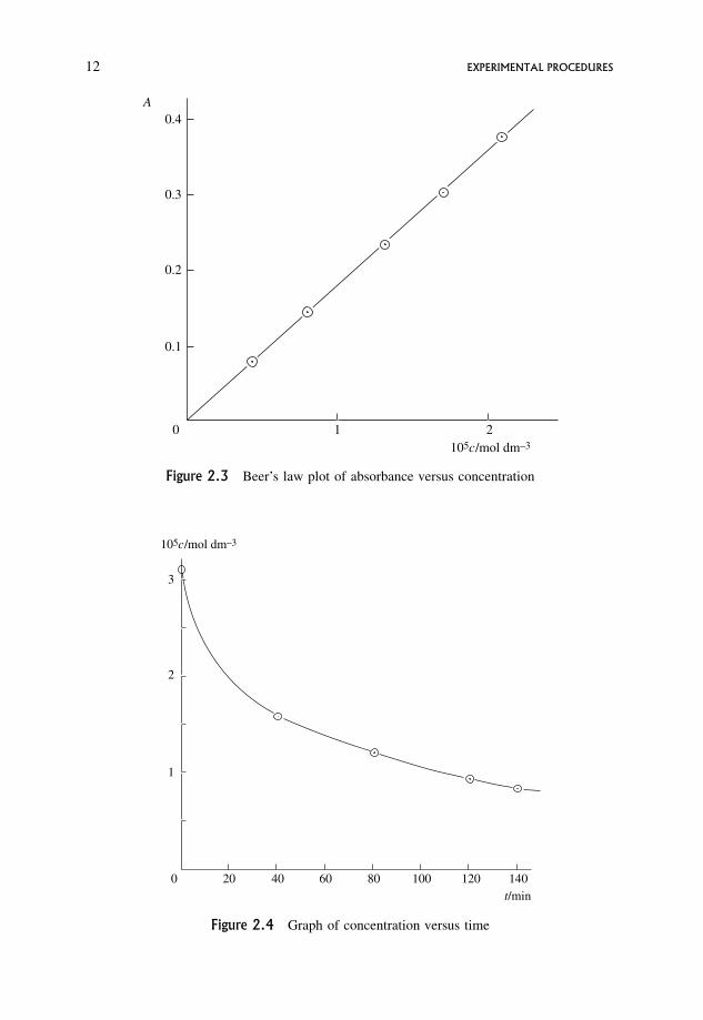
105c/mol dm–3
0
1
2
3
20 40 60 80 100 120 140t/min
Figure 2.4 Graph of concentration versus time
10
0.1
0.2
0.3
0.4
2105c/mol dm–3
A
Figure 2.3 Beer’s law plot of absorbance versus concentration
12 EXPERIMENTAL PROCEDURES
The necessity of making measurements at two wavelengths can be overcome for
gases by using lasers, which have highly defined frequencies compared with the
conventional radiation used in standard absorption analyses. Different species will
absorb at different frequencies. A laser has such a precise frequency that it will only
excite the species which absorbs at precisely that frequency, and no other. Hence
close lying absorptions can be easily separated. This gives a much greater capacity for
singling and separating out absorptions occurring at very closely spaced frequencies;
see Section 2.1.4 below.
Highly sensitive detectors, coupled with the facility to store each absorption signal
digitally for each separate analysis time in a microcomputer, have enabled absorbance
changes as small as 0.001 to be accurately measured.
Spectroscopic techniques are often linked to chromatograph columns for separation
of components, or to flow systems, flash photolysis systems, shock tubes, molecular
beams and other techniques for following reaction.
2.1.4 Lasers
Lasers cover the range from microwave through infrared and visible to the UV. The
following lists the properties of lasers which are of importance in kinetics.
1. Lasers are highly coherent beams allowing reflection through the reaction cell
very many times. This increases the path length and hence the sensitivity.
2. Conventional monochromatic radiation has a span of frequencies, and will thus
excite simultaneously all chemical species which absorb within that narrow range.
Lasers have a precisely defined frequency. This allows species with absorptions
close to each other to be identified and monitored by separate lasers, or by a
tunable laser, in contrast to the indiscriminate absorption which would occur with
conventional sources of radiation.
3. In any spectrum the intensity of absorption is proportional to the concentration of
the molecule in the energy level which is being excited. This is generally
the ground state. If the concentration is very low, as is the case for many gas
phase intermediates, then the intensity of absorption may not be measurable. The
same problem arises in fluorescence where the intensity is proportional to the
concentration of the molecule in the level to which it has been previously excited.
Lasers, on the other hand, have a very high intensity, allowing accurate
concentration determination of intermediates present in very, very low concentra-
tion, and enabling short lived species and processes occurring within 10�15 second
to be picked up. Low intensity conventional sources of radiation cannot do this.
4. Lasers can follow reactions of the free radical and short-lived intermediates found
in complex reactions. Many intermediates in complex gas phase reactions are
DETECTION, IDENTIFICATION AND ESTIMATION OF CONCENTRATION OF SPECIES PRESENT 13
highly reactive and are removed from the reaction almost as soon as they are
formed. If the rate at which they are produced is almost totally balanced by the
total rate of their removal, then the intermediates are present in very, very low and
almost constant concentrations. If these conditions are met, the species are said to
be in steady state concentrations. Since rates of reactions are followed by studying
how concentration varies with time, and since the concentrations of these steady
state intermediates do not change with time, then the rates of their formation and
removal cannot be studied. In conventional kinetic experiments it is impossible to
study these species directly because steady state concentrations remain virtually
constant throughout a kinetic experiment. If these species are produced in
isolation in high concentrations their decay or build-up with time can be studied.
With flash and laser photolysis (Sections 2.5.2 and 2.5.3), high intensity photolytic
flashes produce radicals in high concentrations well above low steady state
concentrations. Subsequent reactions of specific radicals can then be studied
under non-steady state conditions. In flash photolysis, the higher the intensity of
the flash the longer is its duration, limiting the highest intensities to those giving
flashes of around 10�6 s. This limits the accessible time span of reactions to those
with lifetimes greater than this. This limitation does not occur with lasers, and
high intensity flashes of 10�15 s duration are now possible.
5. Early lasers gave single pulses of short duration, e.g. 10�9 s. Pulsed lasers give a
train of equally spaced, high intensity, short duration pulses with intervals ranging
from 10�9 to 10�12 to 10�15 s. These can be used as probes to monitor the changes
in concentration during very fast reactions which are over in times as short as 10�9
to 10�12 s. Isolation of one of the pulses is now possible, giving a single very short
duration initial photolysing flash.
2.1.5 Fluorescence
The frequencies and intensities of fluorescence enable identification and concentra-
tion determinations to be made. The technique is often around 104 times as sensitive
as infra-red, visible or UV absorption spectrophotometry.
In absorption it is a difference in intensity which is being measured (Section 2.1.3).
In absorption the intensity depends on the ground state concentration, and if this is
low then the absorption of radiation is low and accurate measurement is difficult. The
amount absorbed¼ I0 � If . If the change in intensity is small then I0 � If � 0, and no
absorption will be found.
In fluorescence it is the actual intensity of the emitted radiation which is being
measured against a zero background, and this is much easier to measure.
Fluorescence intensity depends on the intensity of the exciting radiation, and also
depends on the concentration of the ground state prior to excitation. Calibration is
necessary unless the reaction is first order (Section 2.1.3).
14 EXPERIMENTAL PROCEDURES
In fluorescence experiments only a small proportion of the incident radiation
results in fluorescence, and so a very intense source of incident radiation is required.
Modern lasers do this admirably, and fluorescence techniques are now routine for
determining very low concentrations.
By using lasers of suitable frequency, fluorescence can be extended into the infra-
red and microwave. Offshoots of laser technology include resonance fluorescence for
detecting atoms, and laser magnetic resonance for radicals.
2.1.6 Spin resonance methods: nuclear magnetic resonance (NMR)
In optical spectroscopy the concentration of an absorbing species can be followed by
monitoring the change in intensity of the signal with time. The same can be done in
NMR spectroscopy, but with limitations as indicated.
For the kineticist, the major use of NMR spectroscopy lies in identifying products
and intermediates in reaction mixtures. Concentrations greater than 10�5 mol dm�3
are necessary for adequate absorption, so low concentration intermediates cannot be
studied.
NMR spectra show considerable complexity, which makes the spectra unambig-
uous, highly characteristic and immediately seen to be unique. This dramatically
increases the value of NMR spectra for identification.
2.1.7 Spin resonance methods: electron spin resonance (ESR)
ESR is an excellent way to study free radicals and molecules with unpaired electrons
present in complex gas reactions, and is used extensively by gas phase kineticists
since it is the one technique which can be applied so directly to free radicals. It is also
used in kinetic studies of paramagnetic ions such as those of transition metals. Again
the change in intensity of the signal from the species can be monitored with time.
Chromatographic techniques are often used to separate free radicals formed in
complex gas reactions, and ESR is used to identify them. The extreme complexity of
the spectra results in a unique fingerprint for the substance being analysed. With ESR
it is possible to detect radicals and other absorbing species in very, very low amounts
such as 10�11 to 10�12 mol, making it an ideal tool for detecting radical and triplet
intermediates present in low concentrations in chemical reactions.
2.1.8 Photoelectron spectroscopy and X-ray
photoelectron spectroscopy
Two more modern spectroscopic techniques for detection, identification and con-
centration determination are photoelectron spectroscopy and X-ray photoelectron
spectroscopy. Essentially these techniques measure how much energy is required to
DETECTION, IDENTIFICATION AND ESTIMATION OF CONCENTRATION OF SPECIES PRESENT 15
remove an electron from some orbital in a molecule, and a photoelectron spectrum
shows a series of bands, each one corresponding to a particular ionization energy.
This spectrum is highly typical of the molecule giving the spectrum, and identifica-
tion can be made. At present the method is in its infancy, and a databank of spectra
specific to given molecules must be produced before the technique can rival e.g. infra-
red methods.
When X-rays are used rather than vacuum UV radiation, electrons are emitted from
inner orbitals, and the spectrum obtained reflects this. These spectra also give much
scope as an analytical technique.
Worked Problem 2.2
Question. Suggest ways of detecting and measuring the concentration of the
following.
1. The species in the gas phase reaction
Br� þ HCl! HBrþ Cl�
2. The many radical species formed in the pyrolysis of an organic hydrocarbon.
3. The blood-red ion pair FeSCN2þ formed by the reaction
Fe3þðaqÞ þ SCN�ðaqÞ ! �� FeSCN2þðaqÞ
4. The catalytic species involved in the acid-catalysed hydrolysis of an ester in
aqueous solution.
5. The charged species in the gas phase reaction
Nþ�2 þ H2 ! N2Hþ þ H�
6. A species whose concentration is 5� 10�10 mol dm�3.
7. The species involved in the reaction
H2OðgÞ þ D2ðgÞ ! HDOðgÞ þ HDðgÞAnswer.
1. Br� and Cl� are radicals: detection and concentration determination by ESR.
HCl and HBr are gaseous: spectroscopic (IR) detection and estimation.
2. Separate by chromatography, detect and analyse spectroscopically or by mass
spectrometry.
3. The ion pair is coloured: spectrophotometry for both detection and estimation.
4. The catalyst is H3Oþ(aq): estimated by titration with OH�(aq).
16 EXPERIMENTAL PROCEDURES
5. Nþ�2 and N2Hþ are ions in the gas phase: mass spectrometry for detection and
estimation.
6. This is a very low concentration species: detection and estimation by laser
induced fluorescence.
7. Three of the species involve deuterium: mass spectrometry is ideal, and can also
be used for H2O.
2.2 Measuring the Rate of a Reaction
Rates of reaction vary from those which seem to be instantaneous, e.g. reaction of
H3Oþ(aq) with OH�(aq), to those which are so slow that they appear not to occur,
e.g. conversion of diamond to graphite. Intermediate situations range from the
slow oxidation of iron (rusting) to a typical laboratory experiment such as the
bromination of an alkene. But in all cases the reactant concentration shows a
smooth decrease with time, and the reaction rate describes how rapidly this decrease
occurs.
The reactant concentration remaining at various times is the fundamental quantity
which requires measurement in any kinetic study.
2.2.1 Classification of reaction rates
Reactions are roughly classified as fast reactions – and the rest. The borderline is
indistinct, but the general consensus is that a ‘fast’ reaction is one which is over in one
second or less. Reactions slower than this lie in the conventional range of rates, and
any of the techniques described previously can be adapted to give rate measurements.
Fast reactions require special techniques.
A very rough general classification of rates can also be given in terms of the time
taken for reaction to appear to be virtually complete, or in terms of half-lives.
Type of reaction Time span for apparent completion Half-life
very fast rate microseconds or less 10�12 to 10�6 second
fast rate seconds 10�6 to 1 second
moderate rate minutes or hours 1 to 103 second
slow rate weeks 103 to 106 second
very slow rate weeks or years >106 second
MEASURING THE RATE OF A REACTION 17
The half-life is the time taken for the concentration to drop to one-half of its value.
If the concentration is 6� 10�2 mol dm�3, then the first half-life is the time taken for
the concentration to fall to 3� 10�2 mol dm�3. The second half-life is the time taken
for the concentration to fall from 3� 10�2 mol dm�3 to 1:5� 10�2 mol dm�3, and
so on.
The dependence of the half-life on concentration reflects the way in which the rate
of reaction depends on concentration.
Care must be taken when using the half-life classification. First order reactions are
the only ones where the half-life is independent of concentration (Sections 3.10.1,
3.11.1 and 3.12.1).
Worked Problem 2.3
Question. If reaction rate / [reactant]2, the half-life, t1/2 / 1/conc. Such a
reaction is called second order (Sections 3.11 and 3.11.1). For a first order reaction,
reaction rate / [reactant] and the half-life is independent of concentration (Sections
3.10 and 3.10.1).
(a) Show how it is possible to bring a fast second order reaction into the
conventional rate region.
(b) Show that this is not possible for first order reactions.
Answer.
(a) If the initial concentration of reactant is decreased by e.g. a factor of 103, then
the half-life is increased by a factor of 103, and if the decrease is by a factor of
106 the half-life increases by a factor of 106. This latter decrease could bring a
reaction with a half-life of 10�4 s into the moderate rate category, with half-life
now 102 s.
(b) Since the half-life for a first order reaction is independent of concentration,
there is no scope for increasing the half-life by altering the initial concentration.
2.2.2 Factors affecting the rate of reaction
� The standard variables are concentration of reactants, temperature and catalyst,
inhibitor or any other substance which affects the rate.
� Chemical reactions are generally very sensitive to temperature and must be
studied at constant temperature.
18 EXPERIMENTAL PROCEDURES
� Rates of reactions in solution and unimolecular reactions in the gas phase are
dependent on pressure.
� Some gas phase chain reactions have rates which are affected by the surface of the
reaction vessel. Heterogeneous catalysis occurs when a surface increases the rate
of the reaction.
� Photochemical reactions occur under the influence of radiation. Conventional
sources of radiation, and modern flash and laser photolysis techniques, are both
extensively used.
� Change of solvent, permittivity, viscosity and ionic strength can all affect the rates
of reactions in solution.
2.2.3 Common experimental features for all reactions
� Chemical reactions must be studied at constant temperature, with control accurate
to � 0.01 �C or preferably better. The reactants must be very rapidly brought to
the experimental temperature at zero time so that reaction does not occur during
this time.
� Mixing of the reactants must occur very much faster than reaction occurs.
� The start of the reaction must be pinpointed exactly and accurately. A stop-watch
is adequate for timing conventional rates; for faster reactions electronic devices
are used. If spectroscopic methods of analysis are used it is simple to have flashes
at very short intervals, e.g. 10�6 s, while with lasers intervals of 10�12 s are
common. Recent advances give intervals of 10�15 s.
� The method of analysis must be very much faster than the reaction itself, so that
virtually no reaction will occur during the period of concentration determination.
2.2.4 Methods of initiation
Normally, thermal initiation is used and the critical energy is acquired by collisions.
In photochemical initiation the critical energy is accumulated by absorption of
radiation. This can only be used if the reactant molecule has a sufficiently strong
absorption in an experimentally accessible region, though modern laser techniques
for photochemical initiation increase the scope considerably.
Absorption of radiation excites the reactant to excited states, from which the
molecule can be disrupted into various radical fragments. Conventional sources produce
steady state concentrations. Flash and laser sources produce much higher concentra-
tions, enabling more accurate concentration determination, and allowing monitoring
of production and removal by reaction of these radicals; this is something which is
not possible with either thermal initiation or conventional photochemical initiation.
MEASURING THE RATE OF A REACTION 19
Lasers have such a high intensity that they can give significant absorption of
radiation, even though " for the absorbing species and its concentration are both very
low. With conventional sources, absorption will be very low, if only one or other of "
and the concentration is low. The crucial point is that the absorbance also depends on
the intensity of the exciting source, and so with lasers this can outweigh a low
concentration and/or a low ".Other useful features of photochemical methods include the following. They
� enable reaction to occur at temperatures at which the thermal reaction does not
occur,
� allow the rate of initiation to be varied at constant temperature, impossible with
thermal initiation,
� allow the rate of initiation to be held constant while the temperature is varied, so
that the temperature effects on the subsequent reactions can be studied indepen-
dently of the rate of initiation (again this is impossible in the thermal reaction) and
� give selective initiation. Frequencies can be chosen at which known excited states
are produced, and the rates of reaction of these excited states can then be studied.
Thermal initiation is totally unselective.
Radiochemical and electric discharge initiation are also used, though these are
much less common. These are much higher energy sources, and they have a much
more disruptive effect on the reactant molecules, producing electrons, atoms, ions and
highly excited molecular and radical species.
2.3 Conventional Methods of Following a Reaction
These determine directly changes in concentrations of reactants and products with
time, but they may have the disadvantages of sampling and speed of analysis.
When reaction is sufficiently fast to result in significant reaction occurring during
the time of sampling and analysis, the rate of reaction is slowed down by reducing the
temperature of the sample drastically, called ‘quenching’; reaction rate generally
decreases dramatically with decreasing temperature. Alternatively, reaction can be
stopped by adding a reagent which will react with the remaining reactant. The amount
of this added reagent can be found analytically, and this gives a measure of the
amount of reactant remaining at the time of addition.
2.3.1 Chemical methods
These are mainly titration methods and they can be highly accurate. They are
generally reserved for simple reactions in solution where either only the reactant or
20 EXPERIMENTAL PROCEDURES
the product concentrations are being monitored. Here sampling errors and speed of
analysis are crucial. Chemical methods have been largely superseded by modern black
box techniques, though, in certain types of solution reaction, they can still be very useful.
Worked Problem 2.4
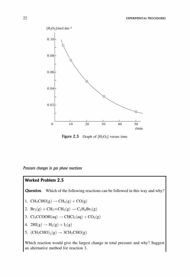
Question. The catalysed decomposition of hydrogen peroxide, H2O2, is easily
followed by titrating 10.0 cm3 samples with 0.0100 mol dm�3 KMnO4 at various
times.
2H2O2ðaqÞ ! 2H2Oð1Þ þ O2ðgÞ
time=min 5 10 20 30 50
volume of 0:0100 mol dm�3 KMnO4=cm3 37:1 29:8 19:6 12:3 5:0
5=2H2O2ðaqÞ þMnO�4 ðaqÞ þ 3HþðaqÞ !Mn2þðaqÞ þ 5=2O2ðgÞ þ 4H2Oð1Þ
1 mol MnO�4 reacts with 5/2 mol H2O2
Calculate the [H2O2] at the various times, and show that these values lie on a
smooth curve when plotted against time.
Answer.
104 � number of mol MnO�4 used 3:71 2:98 1:96 1:23 0:50
104 � number of mol H2O2 present
in sample9:28 7:45 4:90 3:08 1:25
102 � ½H2O2=mol dm�3 9:28 7:45 4:90 3:08 1:25
A graph of [H2O2] versus time is a smooth curve showing the progressive decrease
in reactant concentration with time (Figure 2.5).
2.3.2 Physical methods
These use a physical property dependent on concentration and must be calibrated, but
are still much more convenient than chemical methods. Measurement can often be
made in situ, and analysis is often very rapid. Automatic recording gives a continuous
trace. It is vital to make measurements faster than reaction is occurring.
The following problems illustrate typical physical methods used in the past.
CONVENTIONAL METHODS OF FOLLOWING A REACTION 21
Pressure changes in gas phase reactions
Worked Problem 2.5
Question. Which of the following reactions can be followed in this way and why?
1. CH3CHOðgÞ ! CH4ðgÞ þ COðgÞ
2. Br2ðgÞ þ CH2����CH2ðgÞ ! C2H4Br2ðgÞ
3. Cl3CCOOHðaqÞ ! CHCl3ðaqÞ þ CO2ðgÞ
4. 2HIðgÞ ! H2ðgÞ þ I2ðgÞ
5. ðCH3CHOÞ3ðgÞ ! 3CH3CHOðgÞ
Which reaction would give the largest change in total pressure and why? Suggest
an alternative method for reaction 3.
[H2O2]/mol dm–3
0
0.02
0.04
0.06
0.08
0.10
10 20 30 40 50t/min
Figure 2.5 Graph of [H2O2] versus time
22 EXPERIMENTAL PROCEDURES
Answer. This method can be used for reactions which occur with an overall
change in the number of molecules in the gas phase and which consequently show
a change in total pressure with time.
pV ¼ nRT and p / n if V and T are constant ð2:11Þ
1. Gives an increase in the number of gaseous molecules: pressure increases.
2. Pressure decreases with time.
3. Pressure increases with time.
4. Pressure remains constant, so this method cannot be used.
5. Pressure increases.
Reaction 5 gives the greatest change in the number of molecules in the gas phase,
and hence the largest change in pressure.
In reaction 3, CO2 is the only gaseous species present and the reaction could be
followed by measuring the volume of gas evolved at constant pressure with time.
An actual problem makes the stoichiometric arguments clearer.
Worked Problem 2.6
Question. The gas phase decomposition of ethylamine produces ethene and
ammonia,
C2H5NH2ðgÞ ! C2H4ðgÞ þ NH3ðgÞ
If p0 is the initial pressure of reactant and ptotal is the total pressure at time t, show
how the partial pressure of reactant remaining at time t can be found. Using this and
the following data, find the partial pressure of C2H5NH2 remaining at the various
times, and plot an appropriate graph showing the progress of reaction.
What would the final pressure be?
The following total pressures were found for a reaction at 500 �C with an initial
pressure of pure ethylamine equal to 55 mmHg.
ptotal
mm Hg55 64 72 89 93
time
min0 2 4 10 12
CONVENTIONAL METHODS OF FOLLOWING A REACTION 23
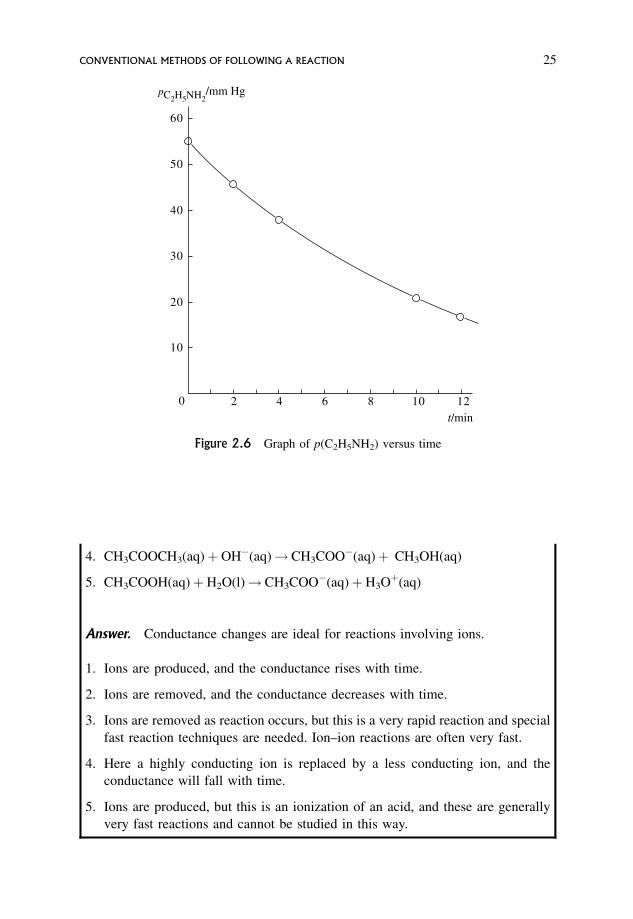
Answer. If p0 is the initial pressure of ethylamine, and an amount of ethylamine
decomposes so that the decrease in its partial pressure is y, then at time t there will
be p0 � y of ethylamine left, y of C2H4 formed and y of NH3 formed.
; total pressure at time t;
ptotal ¼ p0 � yþ yþ y
¼ p0 þ y ð2:12Þ
; y ¼ ptotal � p0 ð2:13Þ
; pðC2H5NH2Þremaining ¼ p0 � y
¼ 2p0 � ptotal ð2:14Þ
Using this gives
ptotal
mmHg55 64 72 89 93
pðC2H5NH2Þ ¼2p0 � ptotal
mmHg55 46 38 21 17
time
min0 2 4 10 12
When reaction is over, the total pressure¼ p(C2H4)þ p(NH3)¼ 2p0¼ 110 mmHg.
A graph of p(C2H5NH2)remaining versus time is a smooth curve (Figure 2.6).
Conductance methods
These are useful when studying reactions involving ions. Again this can be illustrated
by a problem.
Worked Problem 2.7
Question. Which of the following reactions can be studied in this way, and why?
1. (CH3)3CCl(aq)þH2O(l)! (CH3)3COH(aq)þHþ(aq)þ Cl�(aq)
2. NHþ4 (aq)þOCN�(aq)! CO(NH2)2(aq)
3. H3Oþ(aq)þOH�(aq)! 2H2O(l)
24 EXPERIMENTAL PROCEDURES
4. CH3COOCH3(aq)þOH�(aq)! CH3COO�(aq)þ CH3OH(aq)
5. CH3COOH(aq)þH2O(l)! CH3COO�(aq)þH3Oþ(aq)
Answer. Conductance changes are ideal for reactions involving ions.
1. Ions are produced, and the conductance rises with time.
2. Ions are removed, and the conductance decreases with time.
3. Ions are removed as reaction occurs, but this is a very rapid reaction and special
fast reaction techniques are needed. Ion–ion reactions are often very fast.
4. Here a highly conducting ion is replaced by a less conducting ion, and the
conductance will fall with time.
5. Ions are produced, but this is an ionization of an acid, and these are generally
very fast reactions and cannot be studied in this way.
0
10
20
30
40
50
60
2 4 6 8 10 12
pC2H5NH2/mm Hg
t/min
Figure 2.6 Graph of p(C2H5NH2) versus time
CONVENTIONAL METHODS OF FOLLOWING A REACTION 25
pH and EMF methods using a glass electrode sensitive to H3Oþ
Worked Problem 2.8
Question. What types of reaction could be studied in this way?
Answer. In these methods a glass electrode sensitive to H3Oþ enables reactions
which occur with change in [H3Oþ] or a change in [OH�] to be followed with ease.
A pH meter measures pH directly, and a millivoltmeter measures EMFs directly,
and these are related to [H3Oþ], e.g.
� Br2(aq)þ CH3CO-
COCH3(aq)þH2O(l)! CH3COCH2Br(aq)þH3Oþ(aq)þ Br�(aq)
Here H3Oþ(aq) is produced and the pH will decrease with time, with a
corresponding change in EMF,
� CH3COOCH3(aq)þOH�(aq)! CH3COO�(aq)þ CH3OH(aq)
Since OH�(aq) is removed, [H3Oþ] will increase and the pH will decrease with
time, with a corresponding change in EMF and
� CH3COOCH2CH3(aq)þH3Oþ(aq)! CH3COOH(aq)þ CH3CH2OH(aq)
In the acid hydrolyses of esters H3Oþ(aq) is removed, and the pH increases with
time, with a corresponding change in EMF.
Other EMF methods
‘Ion-selective’ electrodes sensitive to ions other than H3Oþ can be used to follow
reactions involving these ions. Silver halide electrodes are used to determine Cl�,
Br�, I� and CN�; lanthanum fluoride to determine F�; Ag2S electrodes to determine
S2�, Agþ and Hg2þ; and electrodes made from a mixture of divalent metal sulphides
and Ag2S are used to determine Pb2þ, Cu2þ and Cd2þ. Other types determine Kþ,
Ca2þ, organic cations, and anions such as NO�3 , ClO�4 and organic anions. Ion-
selective electrodes which monitor the concentration of ions other than H3Oþ or OH�
have proved particularly suitable for biological systems.
A variant on pH methods: the pH-stat and Br2-stat
Monitoring of reactions carried out at constant pH is achieved by a pH-stat device
which adds H3Oþ or OH� automatically to the reaction mixture, depending on
whether H3Oþ or OH� is being used up, and in amounts necessary to maintain
26 EXPERIMENTAL PROCEDURES
constant pH throughout reaction. The volume of solution added is continuously
recorded, and is converted to give the amount of reactant remaining at various times
throughout the reaction. A similar Br2-stat device has been used to follow bromin-
ation reactions. Beside being very useful methods for carrying out routine experi-
ments, pH-stat, Br2-stat or any other kind of stat are very useful for studying reactions
under pseudo-first order conditions where the other reactant is held in constant
concentration.
Chromatographic, mass spectrometric and spectroscopic methods
These can all be used for following the reaction by measuring concentrations at
various times. Often they will be linked up to an automatic recording device and can
be used for measurements in situ. These methods have been discussed earlier.
Dilatometric methods
These measure the change in volume of a solution with time. If this change is
sufficiently large and exaggerated by the use of a dilatometer, it can be used to follow
the rate of reaction. Polymerization reactions are often particularly suited to this
technique.
2.4 Fast Reactions
With fast reactions it is very important to ensure that there is rapid mixing, fast
initiation and fast analysis. Special timing devices are needed. Consequently
techniques special to fast reactions had to be developed.
2.4.1 Continuous flow
Flow systems replace the clock as a timer by a distance along a tube. Two gases or
two solutions are rapidly mixed, and flow rapidly along a tube along which there are
observation chambers at accurately known distances at which the concentration is
determined, either in situ or by leaking samples.
The time for mixing limits the rate of reaction which can be followed, e.g. if
mixing takes 10�3 second, then reactions over in around 10�3 seconds or less cannot
be studied. The moment of mixing gives the zero time. The observation points are at
accurately known distances along the tube and larger distances correspond to longer
reaction times (Figure 2.7).
FAST REACTIONS 27
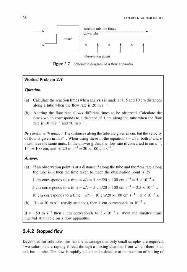
Worked Problem 2.9
Question.
(a) Calculate the reaction times when analysis is made at 1, 5 and 10 cm distances
along a tube when the flow rate is 20 m s�1.
(b) Altering the flow rate allows different times to be observed. Calculate the
times which corresponds to a distance of 1 cm along the tube when the flow
rate is 10 m s�1 and 50 m s�1.
Be careful with units. The distances along the tube are given in cm, but the velocity
of flow is given in m s�1. When using these in the equation t ¼ d=v, both d and v
must have the same units. In the answer given, the flow rate is converted to cm s�1.
1 m¼ 100 cm, and so 20 m s�1¼ 20� 100 cm s�1.
Answer.
(a) If an observation point is at a distance d along the tube and the flow rate along
the tube is v, then the time taken to reach the observation point is d/v,
1 cm corresponds to a time¼ d/v¼ 1 cm/20� 100 cm s�1¼ 5� 10�4 s.
5 cm corresponds to a time¼ d/v¼ 5 cm/20� 100 cm s�1¼ 2.5� 10�3 s.
10 cm corresponds to a time¼ d/v¼ 10 cm/20� 100 cm s�1¼ 5� 10�3 s.
(b) If v¼ 10 m s�1 (easily attained), then 1 cm corresponds to 10�3 s.
If v¼ 50 m s�1 then 1 cm corresponds to 2� 10�4 s, about the smallest time
interval attainable on a flow apparatus.
2.4.2 Stopped flow
Developed for solutions, this has the advantage that only small samples are required.
Two solutions are rapidly forced through a mixing chamber from which there is an
exit into a tube. The flow is rapidly halted and a detector at the position of halting of
observation points
reaction mixture flowsdown tube
mixer
Figure 2.7 Schematic diagram of a flow apparatus
28 EXPERIMENTAL PROCEDURES
the flow gives the concentration. This apparatus in effect acts as an efficient and very
rapid mixing device. The smaller the distance along the tube at which the flow is
halted, the shorter is the time from the start of the reaction at the time of mixing. The
reaction is then followed with time at this point.
The time of analysis must be very rapid. Stopped flow methods always require an
inbuilt timing device, and time intervals at which analysis is made are dictated by the
speed at which successive analyses can be carried out. Spectroscopic methods using
pulsed radiation are very useful here because they can be both analytical and timing
devices.
2.4.3 Accelerated flow
Hypodermic plungers are pushed into syringes increasingly rapidly, and so accelerate
the flow as the mixed reactants pass out of the mixing chamber. Consequently, the
velocity with which the mixed reactants emerge from the mixing chamber increases
with time. When the mixture passes a fixed point on the tube, it will have been
reacting for progressively shorter times. Only small samples are required, but fast
detection is vital.
Worked Problem 2.10
Question. A reaction is carried out in an accelerated flow tube and observations
are made spectrophotometrically.
If the initial flow velocity is 400 cm s�1, calculate the time to reach an observation
point 1 cm along the reaction tube. If the acceleration is such that the velocity
increases progressively to 800, 1200 and 1600 cm s�1, calculate the reaction times
corresponding to these flow rates. If the absorbances corresponding to these times
are 0.124, 0.437, 0.655 and 0.812, draw a graph showing the progress of reaction.
Answer. For observation at 1 cm along the tube
v
cm s�1400 800 1200 1600
time
ms2:50 1:25 0:83 0:625
A 0:124 0:437 0:655 0:812
For a graph of A versus time, see Figure 2.8.
2.4.4 Some features of flow methods
Analysis is generally spectroscopic and done in situ, though mass spectrometry, chro-
matography and conductivity methods have been used. Gas and liquid phase reactions
FAST REACTIONS 29
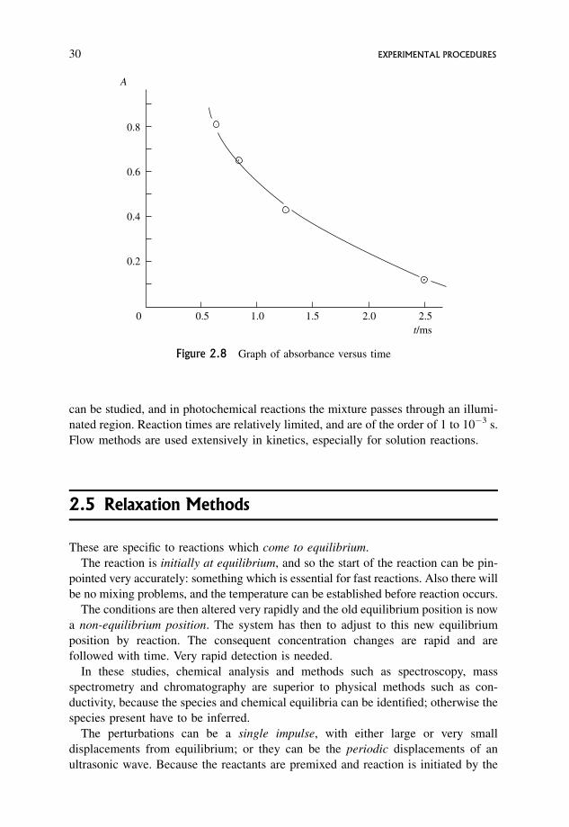
can be studied, and in photochemical reactions the mixture passes through an illumi-
nated region. Reaction times are relatively limited, and are of the order of 1 to 10�3 s.
Flow methods are used extensively in kinetics, especially for solution reactions.
2.5 Relaxation Methods
These are specific to reactions which come to equilibrium.
The reaction is initially at equilibrium, and so the start of the reaction can be pin-
pointed very accurately: something which is essential for fast reactions. Also there will
be no mixing problems, and the temperature can be established before reaction occurs.
The conditions are then altered very rapidly and the old equilibrium position is now
a non-equilibrium position. The system has then to adjust to this new equilibrium
position by reaction. The consequent concentration changes are rapid and are
followed with time. Very rapid detection is needed.
In these studies, chemical analysis and methods such as spectroscopy, mass
spectrometry and chromatography are superior to physical methods such as con-
ductivity, because the species and chemical equilibria can be identified; otherwise the
species present have to be inferred.
The perturbations can be a single impulse, with either large or very small
displacements from equilibrium; or they can be the periodic displacements of an
ultrasonic wave. Because the reactants are premixed and reaction is initiated by the
0 0.5
0.2
0.4
0.6
0.8
1.0 1.5 2.0 2.5
A
t/ms
Figure 2.8 Graph of absorbance versus time
30 EXPERIMENTAL PROCEDURES
impulse, there is no need for rapid mixing. The mixture will also be at the required
temperature.
2.5.1 Large perturbations
Large perturbations using flash or laser photolysis and shock tubes require a new
equilibrium situation to be set up which is far from the initial equilibrium state. These
methods are generally used in gas phase studies, and small perturbations are used for
solutions, though there is nothing constraining the techniques in this way.
2.5.2 Flash photolysis
The reactants are premixed and reaction initiated by an intense flash of radiation
lasting 10�4 to 10�6 s. This disrupts reactant molecules into atoms and radicals in
very high concentrations. The high concentrations of the intermediates produced
make the subsequent kinetic analysis very much easier, and many of these reactions
are often not picked up in low intensity–low concentration photochemical reactions.
The first intense flash is followed by a series of secondary low intensity
flashes which enable the identities and concentrations of the species to be found at
various times, leading ultimately to rate constants for the reactions. Spectroscopic
methods can easily measure intervals of 10�6 s, and lasers can take this down to 10�15 s.
The initial flash must be sufficiently intense to give the high concentrations of
intermediates required, but the higher the intensity of the flash the longer is its
duration. This means that very fast reactions occurring in a time less than or equal to
the duration of the flash will be over by the time the flash is over. A compromise must
be made, and intensities are used so that the flash lasts 10�4 to 10�6 s, and half lives
down to 10�6 s are easy to follow. The secondary flashes are for analysis only and are
of low intensity, so that it is easy to have a flash lasting only 10�6 s.
Flash photolysis greatly increases the number of intermediate reactions able to be
studied. These are generally radical–radical reactions, in contrast to the radical–
molecule reactions which predominate in low intensity photolysis.
The half-lives able to be studied by flash photolysis can be extended to shorter
values in the following modification. Short interval secondary flashes are necessary if
reaction times as short as 10�9 to 10�15 s are to be studied. This is done very
ingeniously by splitting the beam (Figure 2.9). One part of the beam goes through the
reaction mixture and causes photolysis; the other by-passes the reaction mixture, goes
to a movable mirror and is reflected back to the reaction mixture through a fluorescent
solution which converts the beam into continuous radiation in the visible. This is then
used to analyse the mixture spectroscopically. The path lengths of the two parts of the
beam are different. By altering the position of the mirror the time interval between
the first flash and the analytical flash can be varied. For instance, a 30 cm distance
corresponds to an interval of 10�9 s.
RELAXATION METHODS 31
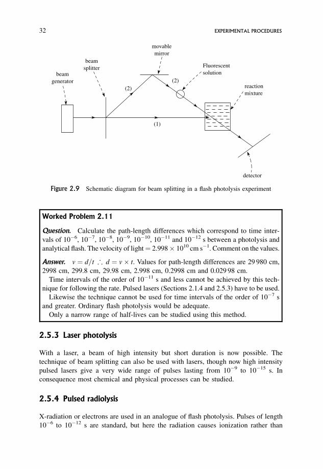
Worked Problem 2.11
Question. Calculate the path-length differences which correspond to time inter-
vals of 10�6, 10�7, 10�8, 10�9, 10�10, 10�11 and 10�12 s between a photolysis and
analytical flash. The velocity of light¼ 2.998� 1010 cm s�1. Comment on the values.
Answer. v ¼ d=t ; d ¼ v� t. Values for path-length differences are 29 980 cm,
2998 cm, 299.8 cm, 29.98 cm, 2.998 cm, 0.2998 cm and 0.029 98 cm.
Time intervals of the order of 10�11 s and less cannot be achieved by this tech-
nique for following the rate. Pulsed lasers (Sections 2.1.4 and 2.5.3) have to be used.
Likewise the technique cannot be used for time intervals of the order of 10�7 s
and greater. Ordinary flash photolysis would be adequate.
Only a narrow range of half-lives can be studied using this method.
2.5.3 Laser photolysis
With a laser, a beam of high intensity but short duration is now possible. The
technique of beam splitting can also be used with lasers, though now high intensity
pulsed lasers give a very wide range of pulses lasting from 10�9 to 10�15 s. In
consequence most chemical and physical processes can be studied.
2.5.4 Pulsed radiolysis
X-radiation or electrons are used in an analogue of flash photolysis. Pulses of length
10�6 to 10�12 s are standard, but here the radiation causes ionization rather than
beamgenerator
beamsplitter
movablemirror
Fluorescentsolution
(2)(2)
(1)
reactionmixture
detector
Figure 2.9 Schematic diagram for beam splitting in a flash photolysis experiment
32 EXPERIMENTAL PROCEDURES
disruption. The range of types of reaction which can now be studied using pulsed
lasers and pulsed radiolysis is extensive.
2.5.5 Shock tubes
A diaphragm with a pressure difference over it of up to about 106 atm is ruptured,
causing a shock wave which passes through a premixed reaction mixture. As the
shock wave passes along the tube it heats the reaction mixture to 104–105 K. The
shock wave reaches the observation point in a very short time (10�6–10�8 s), and all
of the reaction mixture up to this point is then at this very high temperature. This is
zero time for the start of reaction. The tube is able to stay at the high temperature for
around 10�3 s, and all the measurements must be made within that time. The very
high temperature causes disruption of reactant molecules into radicals in very high
concentrations, and these can subsequently react. At the same time the mixture is
driven along the tube by a driver gas. This converts the system to a flow apparatus. As
the mixture is driven past the observation point it will have been reacting for
progressively longer times. Analysis at the observation point will give concentrations
of the species in the mixture corresponding to these times. This often uses lasers at
convenient time intervals ranging from 10�6 s to 10�15 s. When the driver gas reaches
the observation point, the experiment is over. It generally takes 10�3 second between
the arrival of shocked gas and driver gas, and this corresponds to the period of the
high temperature.
Sometimes an alternative procedure places several observation points along the
tube. These correspond to progressively longer times of reaction the further the
observation point is from the diaphragm (Figure 2.10). The calculations are similar to
those in Problem 2.9.
Shock waves combine features of flash photolysis with continuous flow. Though
flash photolysis studies are more flexible and cover a wider range of reaction times,
they are limited to photochemical reactions.
Shock tubes are used for gas reactions. When liquids are used the temperature rises
are small, making the technique much less useful.
2.5.6 Small perturbations: temperature, pressure and
electric field jumps
These single impulse displacements only alter the position of equilibrium provided
certain conditions are met:
(a) temperature jump methods – reaction must have a significant � H;
(b) pressure jump methods – reaction must have a significant � V;
(c) electric field impulse – reaction must involve ionization.
RELAXATION METHODS 33
These techniques involve a sudden increase in temperature, a sudden increase in
pressure and a sudden application of an electric field, respectively.
Table 2.1 summarizes the time taken for the impulse to make its effect, the time
that the effect lasts and hence the time during which concentration measurements
must be made.
For the mathematical analysis of the data to be valid, rates must be studied very
close to equilibrium, and any displacement must be small (see Sections 3.21 and
3.21.1). If a single equilibrium is involved, then the approach to the new equilibrium
position always simulates first order behaviour.
O′ O′′ O′′′O
O′ O′′ O′′′O
O′ O′′ O′′′O
Initial state before rupture of diaphragm:
diaphragm
driver gas, athigh pressure
reaction mixture
Two subsequent situations:
instantaneous positionof shock wave
part of reactionmixture not yetreached by shockwave
heatedpart ofreactionmixture
driver gas
instantaneousposition ofshock wave
part of reactionmixture not yetreached by shockwave
driver gasheated partof reactionmixture
O: observation point
O′, O′′, O′′′: possible additional observation points
Figure 2.10 Schematic diagram of a shock tube apparatus
34 EXPERIMENTAL PROCEDURES
The experimental data is concentration–time data, and integrated rate expressions
give the observed rate constants. The technique can be extended to multi-step
equilibria and to equilibrium reactions with consecutive steps. For multi-step
equilibria, analysis results in a sum of exponentials, which may or may not reduce
to first order.
2.6 Periodic Relaxation Techniques: Ultrasonics
This is the most powerful of the relaxation techniques, partly because it can handle
multi-step equilibria easily, and often gives the relaxation times and the number of
equilibria direct from the actual measurements (Section 3.10.2). It has been used to
study physical processes such as energy transfer and ion solvation, as well as
chemical reactions. This technique is used for reaction times of 1 to 10�10 s.
If passed through a reaction mixture, a sound wave causes a wave of alternating
temperatures which calls for a corresponding wave of new equilibrium positions to be
set up. If the concentrations of species involved in the equilibria can alter rapidly
enough to enable each new equilibrium position to be set up as each new temperature
is attained, then the concentrations and the equilibria can keep in phase with
the periodic displacement. This occurs when the period of the sound wave is large
compared with the relaxation time.
If reaction does not occur fast enough, then the concentration will not alter in phase
with the periodic displacement, the required equilibria for each temperature are not
set up and the concentrations remain approximately constant throughout. This occurs
when the period of the sound wave is very small compared to the relaxation time.
These are two extremes. An intermediate situation, where the period of the sound
wave is comparable to the relaxation time, occurs when reaction is fast enough to
allow the concentrations to alter with time, but the change in concentration is out of
phase with the sound wave. This shows up as an increase in the velocity of sound,
or as a maximum in the absorption of sound by the reaction mixture as the frequency
of the sound wave alters. This is the region where all the useful information is
obtained.
Table 2.1 Single impulse relaxation
Impulse
Time for jump to
occur (s) Change lasts (s)
Observations must
be made in (s)
Temperature 10�6 1 1–10�6
Pressure 10�4 50 50–10�4
Electric 10�8 2� 10�4 2� 10�4–10�8
Shock 10�6 50 50–10�6
PERIODIC RELAXATION TECHNIQUES: ULTRASONICS 35
If there is only one equilibrium, i.e. one relaxation time involved, there is a single
point of inflection on the velocity–frequency diagram, or one maximum in the
absorption of sound–frequency diagram (Figures 2.11 and 2.12). For more than
one equilibrium then there will be a corresponding number of points of inflection, or
maxima (Figures 2.13 and 2.14), provided the relaxation processes are resolved.
These are easily and accurately measured. Sound waves are passed through the
reaction mixture and the velocity of sound, or its absorption, is measured for a series
of frequencies of the sound wave, and a graph drawn. From each point of inflection or
maximum the relaxation time can be found directly and the rate constant calculated
(Table 3.3). Solving the kinetics of complex equilibria is straightforward using
relaxation times, in contrast to the increasing difficulty and eventual impossibility
of using integrated rate equations and concentration data (Section 3.9).
If the relaxation processes are not resolved, best fit computer analysis is used.
Unfortunately, chemical identification of the relaxation process is by far the most
difficult and ambiguous part of the analysis. There are no direct chemical observations.
The magnitude of the relaxation time can often distinguish between physical processes
and chemical reactions, but this does not reveal what the chemical reactions are.
Relaxation times of the order of 10�5 to 10�10 s are usually studied, giving first
order rate constants lying between 105 and 1010 s�1, though slower reactions can
concentrationunable to alter inphase withultrasonic wave
concentrationable to alter inphase withultrasonic wave
concentration altering,but not in phase withultrasonic wave
dispersionregion
frequency
V2
Figure 2.11 Periodic relaxation diagram showing the dependence of the velocity of an ultrasonic
wave through a reaction mixture on its frequency
36 EXPERIMENTAL PROCEDURES
two extremes forone equilibrium
two extremes forone equilibrium
one componentunable to
alter in phase
another componentunable to alterin phase
another componentout of phase,but altering
one componentout of phase, butaltering
all componentsable to alterin phase
onecomponentfalling out
anothercomponentfalling out
dispersionregion dispersion
region
frequency
V2
Figure 2.13 Periodic relaxation for a double equilibrium: diagram for velocity of wave
relaxationabsorption
curve
absorption whichthere would be ifthere were norelaxation process
frequency
absorptionµ
Figure 2.12 Periodic relaxation diagram showing the dependence of the absorption of an
ultrasonic wave through a reaction mixture on its frequency
PERIODIC RELAXATION TECHNIQUES: ULTRASONICS 37
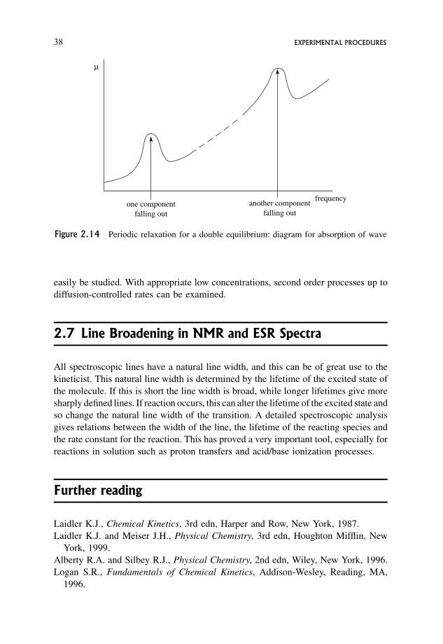
easily be studied. With appropriate low concentrations, second order processes up to
diffusion-controlled rates can be examined.
2.7 Line Broadening in NMR and ESR Spectra
All spectroscopic lines have a natural line width, and this can be of great use to the
kineticist. This natural line width is determined by the lifetime of the excited state of
the molecule. If this is short the line width is broad, while longer lifetimes give more
sharply defined lines. If reaction occurs, this can alter the lifetime of the excited state and
so change the natural line width of the transition. A detailed spectroscopic analysis
gives relations between the width of the line, the lifetime of the reacting species and
the rate constant for the reaction. This has proved a very important tool, especially for
reactions in solution such as proton transfers and acid/base ionization processes.
Further reading
Laidler K.J., Chemical Kinetics, 3rd edn, Harper and Row, New York, 1987.
Laidler K.J. and Meiser J.H., Physical Chemistry, 3rd edn, Houghton Mifflin, New
York, 1999.
Alberty R.A. and Silbey R.J., Physical Chemistry, 2nd edn, Wiley, New York, 1996.
Logan S.R., Fundamentals of Chemical Kinetics, Addison-Wesley, Reading, MA,
1996.
one componentfalling out
another componentfalling out
frequency
µ
Figure 2.14 Periodic relaxation for a double equilibrium: diagram for absorption of wave
38 EXPERIMENTAL PROCEDURES
� Nicholas J., Chemical Kinetics, Harper and Row, New York, 1976.
� Wilkinson F., Chemical Kinetics and Reaction Mechanisms, Van Nostrand Rein-
hold, New York, 1980.� Out of print, but should be in university libraries.
Further problems
1. Suggest ways for determining the rate of the following reactions.
� Bromination of CH3CH����CH2 in aqueous solution.
� Reaction of C2H�5 with CH3COCH3 in the gas phase.
� A polymerization reaction.
� Iodination of CH3COCH3.
� 2NO(g)þ 2H2(g)!N2(g)þ 2H2O(g)
� A reaction in solution with a half-life of 10�4 s.
� K�(g)þ CH3I(g)!KI(g)þ CH�3(g)
� C6H5Nþ2 (aq)þH2O(l)! C6H5OH(aq)þHþ(aq)þN2(g)
� Aþ B ! � C ! � D ! � Eþ F
� S2O2�8 ðaqÞ þ 2I�ðaqÞ ! 2SO2�
4 ðaqÞ þ I2ðaqÞ
� A reaction with a half-life of 10�9 s.
2. The following table gives the absorbances for various concentrations of a solution.
A 1 cm optical cell is used. Use this to calculate the molar absorption coefficient
for the solute.
conc:
mol dm�30:0045 0:0105 0:0140 0:0190
A 0:380 0:899 1:195 1:615
The kinetics of a reaction involving this solute as reactant, in which only the reactant
absorbs, gives the following data. Convert this data to [reactant] as a function of time.
A 1:420 1:139 0:904 0:724 0:584
time
s0 100 200 300 400
3. Interpret the spectrum shown in Figure 2.15.
FURTHER PROBLEMS 39
absorption
(a)
(b)(c)
frequency
t = 10 min
absorption
(a)
(b)
(c)
frequency
t = 20 min
absorption
(a)
(b)
(c)
frequency
t = 30 min
Figure 2.15
40 EXPERIMENTAL PROCEDURES
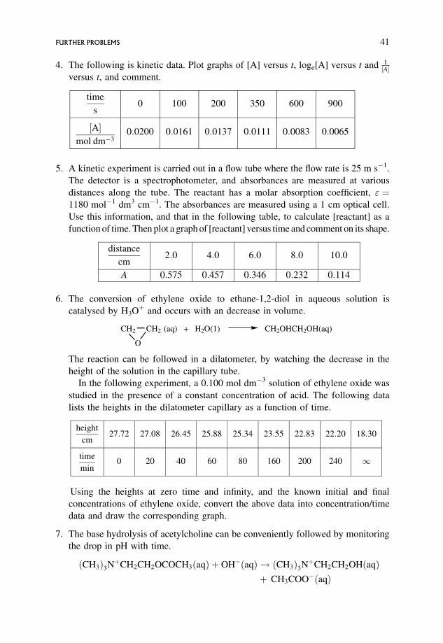
4. The following is kinetic data. Plot graphs of [A] versus t, loge[A] versus t and 1½A
versus t, and comment.
time
s0 100 200 350 600 900
½Amol dm�3
0:0200 0:0161 0:0137 0:0111 0:0083 0:0065
5. A kinetic experiment is carried out in a flow tube where the flow rate is 25 m s�1.
The detector is a spectrophotometer, and absorbances are measured at various
distances along the tube. The reactant has a molar absorption coefficient, " ¼1180 mol�1 dm3 cm�1. The absorbances are measured using a 1 cm optical cell.
Use this information, and that in the following table, to calculate [reactant] as a
function of time. Then plot a graph of [reactant] versus time and comment on its shape.
distance
cm2:0 4:0 6:0 8:0 10:0
A 0:575 0:457 0:346 0:232 0:114
6. The conversion of ethylene oxide to ethane-1,2-diol in aqueous solution is
catalysed by H3Oþ and occurs with an decrease in volume.
CH2
O
CH2 (aq) + H2O(1) CH2OHCH2OH(aq)
The reaction can be followed in a dilatometer, by watching the decrease in the
height of the solution in the capillary tube.
In the following experiment, a 0.100 mol dm�3 solution of ethylene oxide was
studied in the presence of a constant concentration of acid. The following data
lists the heights in the dilatometer capillary as a function of time.
height
cm27:72 27:08 26:45 25:88 25:34 23:55 22:83 22:20 18:30
time
min0 20 40 60 80 160 200 240 1
Using the heights at zero time and infinity, and the known initial and final
concentrations of ethylene oxide, convert the above data into concentration/time
data and draw the corresponding graph.
7. The base hydrolysis of acetylcholine can be conveniently followed by monitoring
the drop in pH with time.
ðCH3Þ3NþCH2CH2OCOCH3ðaqÞ þ OH�ðaqÞ ! ðCH3Þ3NþCH2CH2OHðaqÞþ CH3COO�ðaqÞ
FURTHER PROBLEMS 41
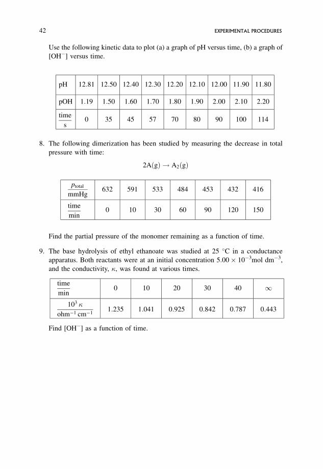
Use the following kinetic data to plot (a) a graph of pH versus time, (b) a graph of
[OH�] versus time.
pH 12:81 12:50 12:40 12:30 12:20 12:10 12:00 11:90 11:80
pOH 1:19 1:50 1:60 1:70 1:80 1:90 2:00 2:10 2:20
time
s0 35 45 57 70 80 90 100 114
8. The following dimerization has been studied by measuring the decrease in total
pressure with time:
2AðgÞ ! A2ðgÞ
ptotal
mmHg632 591 533 484 453 432 416
time
min0 10 30 60 90 120 150
Find the partial pressure of the monomer remaining as a function of time.
9. The base hydrolysis of ethyl ethanoate was studied at 25 �C in a conductance
apparatus. Both reactants were at an initial concentration 5:00� 10�3mol dm�3,
and the conductivity, �, was found at various times.
time
min0 10 20 30 40 1
103 �
ohm�1 cm�11:235 1:041 0:925 0:842 0:787 0:443
Find [OH�] as a function of time.
42 EXPERIMENTAL PROCEDURES
3 The Kinetic Analysis of
Experimental Data
In Chapter 2 methods of following a reaction with time were discussed, and
techniques for probing changes in concentration of reactant remaining at various
times were described. Practice was given at converting the experimental data into
[reactant] left at times throughout the experiment. Graphs of [reactant] versus time
were drawn, and all the kinetic quantities which are described in this book derive
from such basic data.
The data from such experiments must now be manipulated to give quantitative
information about each reaction.
Aims
By the end of this chapter you should be able to
� define the rate of reaction and discuss its dependence on reactant concentration,
� understand the meaning of order and rate constant and determine both fromrate/concentration data,
� know the meaning of half-life,
� find the order and rate constant from concentration/time data using integratedrate expressions,
� understand and use the steady state treatment and
� appreciate the complexities involved in unravelling the kinetics of complexreactions.
An Introduction to Chemical Kinetics. Margaret Robson Wright# 2004 John Wiley & Sons, Ltd. ISBNs: 0-470-09058-8 (hbk) 0-470-09059-6 (pbk)
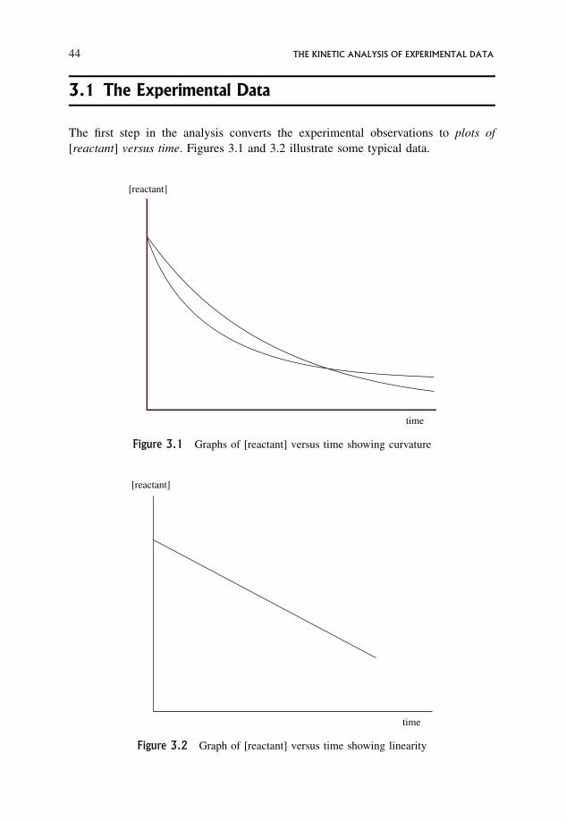
3.1 The Experimental Data
The first step in the analysis converts the experimental observations to plots of
[reactant] versus time. Figures 3.1 and 3.2 illustrate some typical data.
[reactant]
time
Figure 3.1 Graphs of [reactant] versus time showing curvature
[reactant]
time
Figure 3.2 Graph of [reactant] versus time showing linearity
44 THE KINETIC ANALYSIS OF EXPERIMENTAL DATA
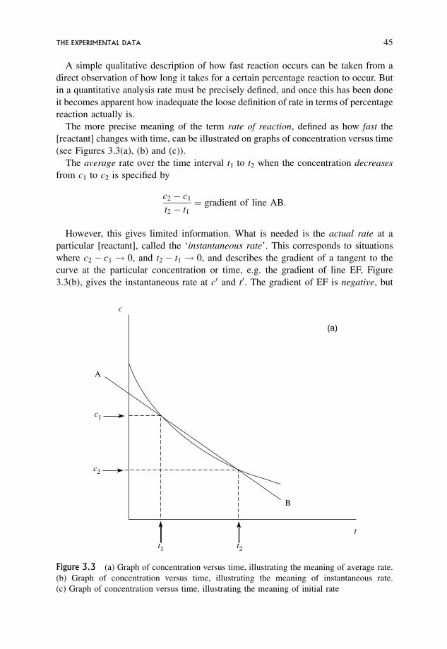
A simple qualitative description of how fast reaction occurs can be taken from a
direct observation of how long it takes for a certain percentage reaction to occur. But
in a quantitative analysis rate must be precisely defined, and once this has been done
it becomes apparent how inadequate the loose definition of rate in terms of percentage
reaction actually is.
The more precise meaning of the term rate of reaction, defined as how fast the
[reactant] changes with time, can be illustrated on graphs of concentration versus time
(see Figures 3.3(a), (b) and (c)).
The average rate over the time interval t1 to t2 when the concentration decreases
from c1 to c2 is specified by
c2 � c1
t2 � t1
¼ gradient of line AB:
However, this gives limited information. What is needed is the actual rate at a
particular [reactant], called the ‘instantaneous rate’. This corresponds to situations
where c2 � c1 ! 0, and t2 � t1 ! 0, and describes the gradient of a tangent to the
curve at the particular concentration or time, e.g. the gradient of line EF, Figure
3.3(b), gives the instantaneous rate at c0 and t0. The gradient of EF is negative, but
c
A
t1 t2
B
t
(a)
c2
c1
Figure 3.3 (a) Graph of concentration versus time, illustrating the meaning of average rate.
(b) Graph of concentration versus time, illustrating the meaning of instantaneous rate.
(c) Graph of concentration versus time, illustrating the meaning of initial rate
THE EXPERIMENTAL DATA 45
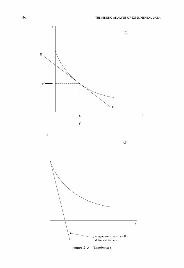
t′
c′
E
F
(b)
c
t
c
t
tangent to curve at t = 0:defines initial rate
(c)
Figure 3.3 (Continued )
46 THE KINETIC ANALYSIS OF EXPERIMENTAL DATA
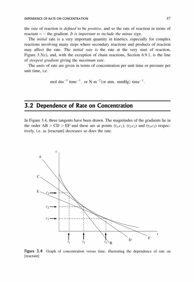
the rate of reaction is defined to be positive, and so the rate of reaction in terms of
reactant¼� the gradient. It is important to include the minus sign.
The initial rate is a very important quantity in kinetics, especially for complex
reactions involving many steps where secondary reactions and products of reaction
may affect the rate. The initial rate is the rate at the very start of reaction,
Figure 3.3(c), and, with the exception of chain reactions, Section 6.9.1, is the line
of steepest gradient giving the maximum rate.
The units of rate are given in terms of concentration per unit time or pressure per
unit time, i.e.
mol dm�3 time�1; or N m�2ðor atm; mmHgÞ time�1:
3.2 Dependence of Rate on Concentration
In Figure 3.4, three tangents have been drawn. The magnitudes of the gradients lie in
the order AB > CD > EF and these are at points (t1,c1), (t2,c2) and (t3,c3) respec-
tively, i.e. as [reactant] decreases so does the rate.
t1
c3
c2
c1
t2 t3 BD F
E
C
A
c
t
Figure 3.4 Graph of concentration versus time, illustrating the dependence of rate on
[reactant]
DEPENDENCE OF RATE ON CONCENTRATION 47
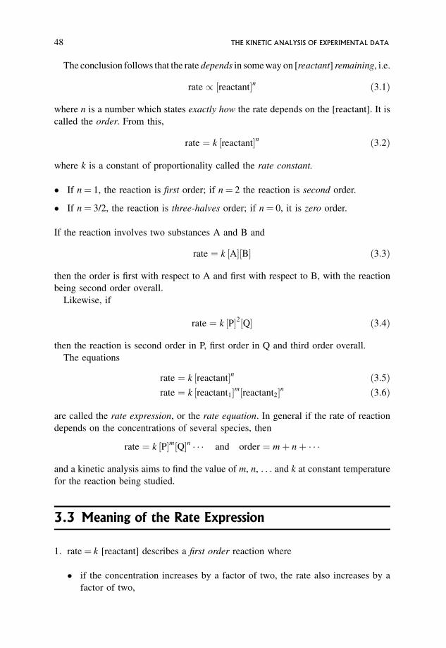
The conclusion follows that the rate depends in some way on [reactant] remaining, i.e.
rate / ½reactantn ð3:1Þ
where n is a number which states exactly how the rate depends on the [reactant]. It is
called the order. From this,
rate ¼ k ½reactantn ð3:2Þ
where k is a constant of proportionality called the rate constant.
� If n¼ 1, the reaction is first order; if n¼ 2 the reaction is second order.
� If n¼ 3/2, the reaction is three-halves order; if n¼ 0, it is zero order.
If the reaction involves two substances A and B and
rate ¼ k ½A½B ð3:3Þ
then the order is first with respect to A and first with respect to B, with the reaction
being second order overall.
Likewise, if
rate ¼ k ½P2½Q ð3:4Þ
then the reaction is second order in P, first order in Q and third order overall.
The equations
rate ¼ k ½reactantn ð3:5Þrate ¼ k ½reactant1m½reactant2n ð3:6Þ
are called the rate expression, or the rate equation. In general if the rate of reaction
depends on the concentrations of several species, then
rate ¼ k ½Pm½Qn � � � and order ¼ mþ nþ � � �
and a kinetic analysis aims to find the value of m, n, . . . and k at constant temperature
for the reaction being studied.
3.3 Meaning of the Rate Expression
1. rate¼ k [reactant] describes a first order reaction where
� if the concentration increases by a factor of two, the rate also increases by a
factor of two,
48 THE KINETIC ANALYSIS OF EXPERIMENTAL DATA
� if the concentration increases by a factor of six, the rate also increases by a
factor of six.
2. rate¼ k [reactant]2 describes a second order reaction where
� if the concentration increases by a factor of two, the rate increases by a factor
of 22, i.e. four,
� if the concentration increases by a factor of six, the rate increases by a factor of
62, i.e. 36.
3. rate¼ k[reactant]0¼ k describes a zero order reaction where
� no matter how the concentration varies, the rate remains constant.
3.4 Units of the Rate Constant, k
These depend on the order of the reaction and are worked out as follows.
� First order reaction:
rate ¼ k ½reactant ð3:7Þk ¼ rate=½reactant ð3:8Þ
Units of k are, therefore,mol dm�3time�1
mol dm�3i.e time�1
� Second order reaction:
rate ¼ k ½reactant2 ð3:9Þ
k ¼ rate=½reactant2 ð3:10Þ
Units of k are, therefore,mol dm�3time�1
mol2 dm�6i.e. mol�1 dm3 time�1
� Zero order reaction:
rate ¼ k ð3:11Þ
Units of k are, therefore, mol dm�3 time�1.
UNITS OF THE RATE CONSTANT, k 49
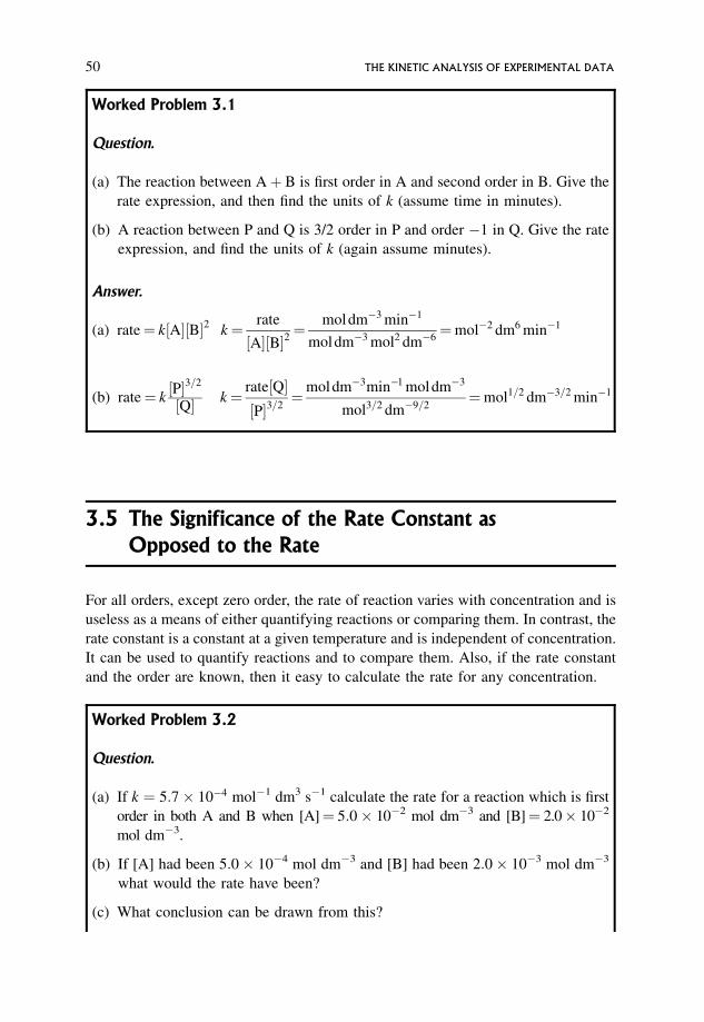
Worked Problem 3.1
Question.
(a) The reaction between Aþ B is first order in A and second order in B. Give the
rate expression, and then find the units of k (assume time in minutes).
(b) A reaction between P and Q is 3/2 order in P and order �1 in Q. Give the rate
expression, and find the units of k (again assume minutes).
Answer.
(a) rate¼ k½A½B2 k¼ rate
½A½B2¼ moldm�3 min�1
moldm�3 mol2 dm�6¼mol�2 dm6 min�1
(b) rate¼ k½P3=2
½Q k¼ rate½Q½P3=2
¼moldm�3min�1 moldm�3
mol3=2 dm�9=2¼mol1=2 dm�3=2 min�1
3.5 The Significance of the Rate Constant as
Opposed to the Rate
For all orders, except zero order, the rate of reaction varies with concentration and is
useless as a means of either quantifying reactions or comparing them. In contrast, the
rate constant is a constant at a given temperature and is independent of concentration.
It can be used to quantify reactions and to compare them. Also, if the rate constant
and the order are known, then it easy to calculate the rate for any concentration.
Worked Problem 3.2
Question.
(a) If k ¼ 5:7 10�4 mol�1 dm3 s�1 calculate the rate for a reaction which is first
order in both A and B when [A]¼ 5:0 10�2 mol dm�3 and [B]¼ 2.0 10�2
mol dm�3.
(b) If [A] had been 5:0 10�4 mol dm�3 and [B] had been 2:0 10�3 mol dm�3
what would the rate have been?
(c) What conclusion can be drawn from this?
50 THE KINETIC ANALYSIS OF EXPERIMENTAL DATA
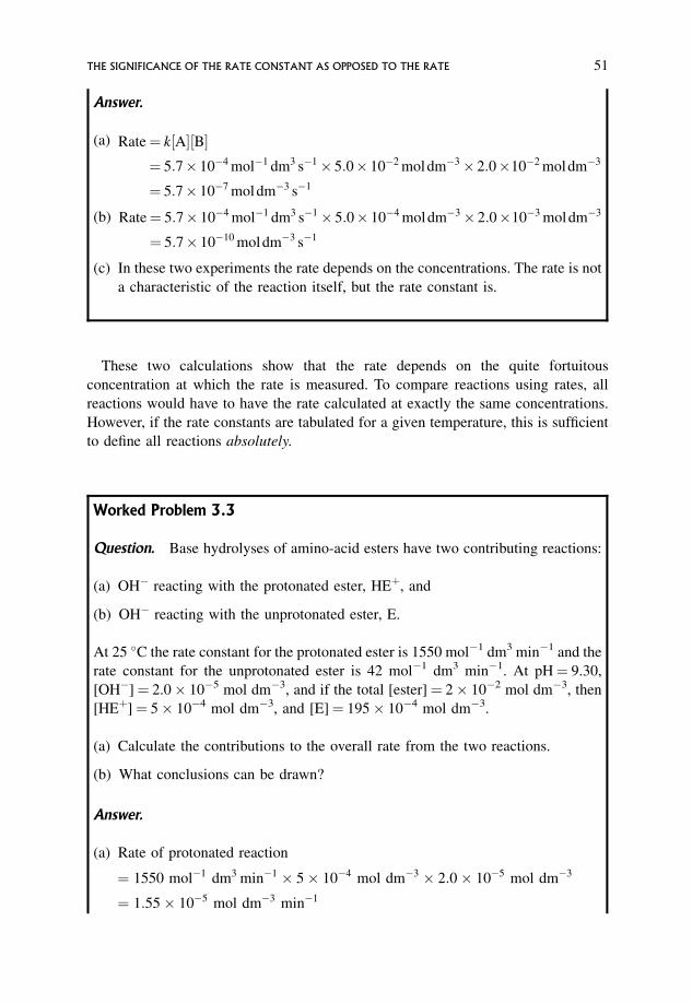
Answer.
(a) Rate¼ k½A½B¼ 5:7 10�4 mol�1 dm3 s�1 5:0 10�2 moldm�3 2:0 10�2 moldm�3
¼ 5:7 10�7 moldm�3 s�1
(b) Rate¼ 5:7 10�4 mol�1 dm3 s�1 5:0 10�4 moldm�3 2:0 10�3 moldm�3
¼ 5:7 10�10 moldm�3 s�1
(c) In these two experiments the rate depends on the concentrations. The rate is not
a characteristic of the reaction itself, but the rate constant is.
These two calculations show that the rate depends on the quite fortuitous
concentration at which the rate is measured. To compare reactions using rates, all
reactions would have to have the rate calculated at exactly the same concentrations.
However, if the rate constants are tabulated for a given temperature, this is sufficient
to define all reactions absolutely.
Worked Problem 3.3
Question. Base hydrolyses of amino-acid esters have two contributing reactions:
(a) OH� reacting with the protonated ester, HEþ, and
(b) OH� reacting with the unprotonated ester, E.
At 25 �C the rate constant for the protonated ester is 1550 mol�1 dm3 min�1 and the
rate constant for the unprotonated ester is 42 mol�1 dm3 min�1. At pH¼ 9.30,
[OH�]¼ 2.0 10�5 mol dm�3, and if the total [ester]¼ 2 10�2 mol dm�3, then
[HEþ]¼ 5 10�4 mol dm�3, and [E]¼ 195 10�4 mol dm�3.
(a) Calculate the contributions to the overall rate from the two reactions.
(b) What conclusions can be drawn?
Answer.
(a) Rate of protonated reaction
¼ 1550 mol�1 dm3 min�1 5 10�4 mol dm�3 2:0 10�5 mol dm�3
¼ 1:55 10�5 mol dm�3 min�1
THE SIGNIFICANCE OF THE RATE CONSTANT AS OPPOSED TO THE RATE 51
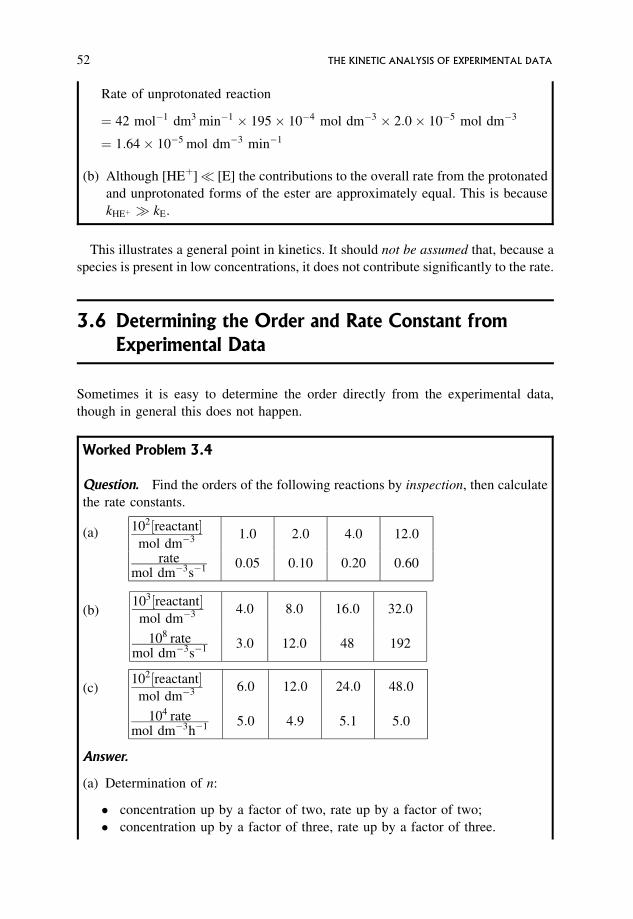
Rate of unprotonated reaction
¼ 42 mol�1 dm3 min�1 195 10�4 mol dm�3 2:0 10�5 mol dm�3
¼ 1:64 10�5 mol dm�3 min�1
(b) Although [HEþ]� [E] the contributions to the overall rate from the protonated
and unprotonated forms of the ester are approximately equal. This is because
kHEþ � kE.
This illustrates a general point in kinetics. It should not be assumed that, because a
species is present in low concentrations, it does not contribute significantly to the rate.
3.6 Determining the Order and Rate Constant from
Experimental Data
Sometimes it is easy to determine the order directly from the experimental data,
though in general this does not happen.
Worked Problem 3.4
Question. Find the orders of the following reactions by inspection, then calculate
the rate constants.
(a) 102½reactantmol dm�3 1:0 2:0 4:0 12:0
ratemol dm�3s�1 0:05 0:10 0:20 0:60
(b)103½reactant
mol dm�3 4:0 8:0 16:0 32:0
108 ratemol dm�3s�1 3:0 12:0 48 192
(c)102½reactant
mol dm�3 6:0 12:0 24:0 48:0
104 ratemol dm�3h�1 5:0 4:9 5:1 5:0
Answer.
(a) Determination of n:
� concentration up by a factor of two, rate up by a factor of two;
� concentration up by a factor of three, rate up by a factor of three.
52 THE KINETIC ANALYSIS OF EXPERIMENTAL DATA
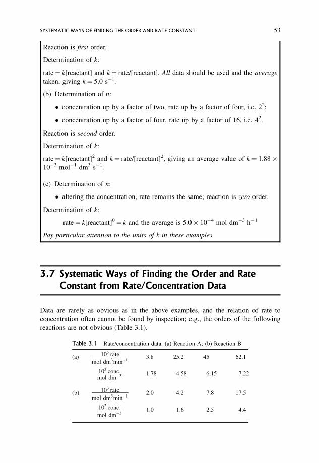
Reaction is first order.
Determination of k:
rate¼ k[reactant] and k¼ rate/[reactant]. All data should be used and the average
taken, giving k¼ 5.0 s�1.
(b) Determination of n:
� concentration up by a factor of two, rate up by a factor of four, i.e. 22;
� concentration up by a factor of four, rate up by a factor of 16, i.e. 42.
Reaction is second order.
Determination of k:
rate¼ k[reactant]2 and k¼ rate/[reactant]2, giving an average value of k¼ 1.88 10�3 mol�1 dm3 s�1.
(c) Determination of n:
� altering the concentration, rate remains the same; reaction is zero order.
Determination of k:
rate¼ k[reactant]0¼ k and the average is 5.0 10�4 mol dm�3 h�1
Pay particular attention to the units of k in these examples.
3.7 Systematic Ways of Finding the Order and Rate
Constant from Rate/Concentration Data
Data are rarely as obvious as in the above examples, and the relation of rate to
concentration often cannot be found by inspection; e.g., the orders of the following
reactions are not obvious (Table 3.1).
Table 3.1 Rate/concentration data. (a) Reaction A; (b) Reaction B
(a) 105 rate
mol dm3min�13.8 25.2 45 62.1
103 conc:mol dm�3 1.78 4.58 6.15 7.22
(b) 103 rate
mol dm3min�12.0 4.2 7.8 17.5
102 conc:
mol dm�31.0 1.6 2.5 4.4
SYSTEMATIC WAYS OF FINDING THE ORDER AND RATE CONSTANT 53
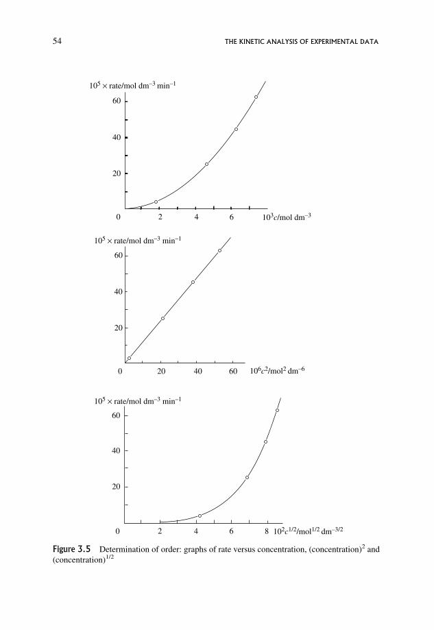
0 2 4 6 103c/mol dm–3
105 × rate/mol dm–3 min–1
60
40
20
106c2/mol2 dm–6
105 × rate/mol dm–3 min–1
0 20 40 60
20
40
60
102c1/2/mol1/2 dm–3/2
105 × rate/mol dm–3 min–1
0
20
40
60
2 64 8
Figure 3.5 Determination of order: graphs of rate versus concentration, (concentration)2 and
(concentration)1/2
54 THE KINETIC ANALYSIS OF EXPERIMENTAL DATA
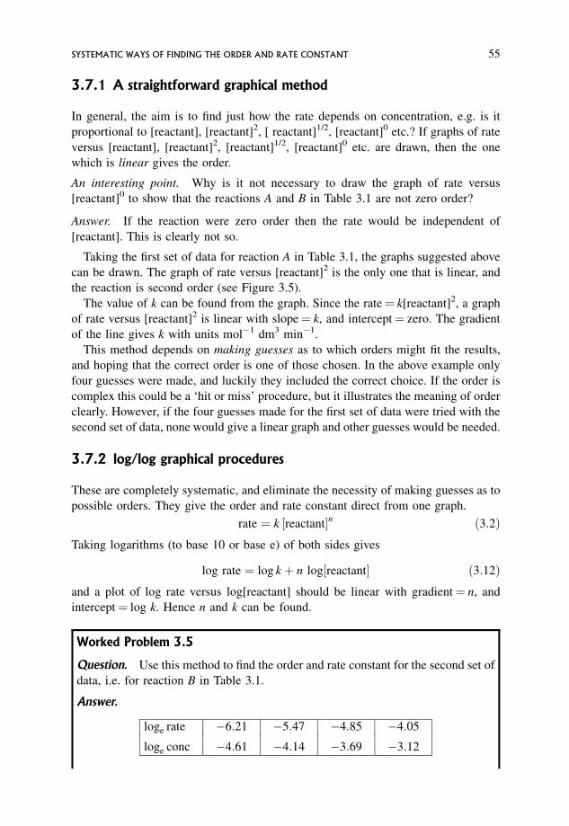
3.7.1 A straightforward graphical method
In general, the aim is to find just how the rate depends on concentration, e.g. is it
proportional to [reactant], [reactant]2, [ reactant]1/2, [reactant]0 etc.? If graphs of rate
versus [reactant], [reactant]2, [reactant]1/2, [reactant]0 etc. are drawn, then the one
which is linear gives the order.
An interesting point. Why is it not necessary to draw the graph of rate versus
[reactant]0 to show that the reactions A and B in Table 3.1 are not zero order?
Answer. If the reaction were zero order then the rate would be independent of
[reactant]. This is clearly not so.
Taking the first set of data for reaction A in Table 3.1, the graphs suggested above
can be drawn. The graph of rate versus [reactant]2 is the only one that is linear, and
the reaction is second order (see Figure 3.5).
The value of k can be found from the graph. Since the rate¼ k[reactant]2, a graph
of rate versus [reactant]2 is linear with slope¼ k, and intercept¼ zero. The gradient
of the line gives k with units mol�1 dm3 min�1.
This method depends on making guesses as to which orders might fit the results,
and hoping that the correct order is one of those chosen. In the above example only
four guesses were made, and luckily they included the correct choice. If the order is
complex this could be a ‘hit or miss’ procedure, but it illustrates the meaning of order
clearly. However, if the four guesses made for the first set of data were tried with the
second set of data, none would give a linear graph and other guesses would be needed.
3.7.2 log/log graphical procedures
These are completely systematic, and eliminate the necessity of making guesses as to
possible orders. They give the order and rate constant direct from one graph.
rate ¼ k ½reactantn ð3:2ÞTaking logarithms (to base 10 or base e) of both sides gives
log rate ¼ log k þ n log½reactant ð3:12Þand a plot of log rate versus log[reactant] should be linear with gradient¼ n, and
intercept¼ log k. Hence n and k can be found.
Worked Problem 3.5
Question. Use this method to find the order and rate constant for the second set of
data, i.e. for reaction B in Table 3.1.
Answer.
loge rate �6:21 �5:47 �4:85 �4:05
loge conc �4:61 �4:14 �3:69 �3:12
SYSTEMATIC WAYS OF FINDING THE ORDER AND RATE CONSTANT 55
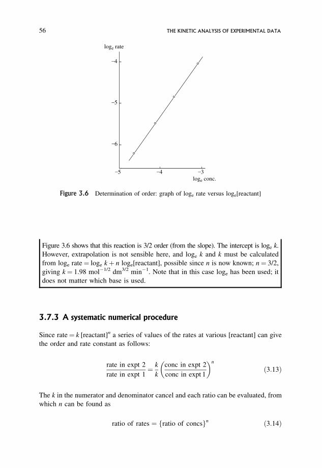
Figure 3.6 shows that this reaction is 3/2 order (from the slope). The intercept is loge k.
However, extrapolation is not sensible here, and loge k and k must be calculated
from loge rate¼ loge kþ n loge[reactant], possible since n is now known; n¼ 3/2,
giving k¼ 1.98 mol�1/2 dm3/2 min�1. Note that in this case loge has been used; it
does not matter which base is used.
3.7.3 A systematic numerical procedure
Since rate¼ k [reactant]n a series of values of the rates at various [reactant] can give
the order and rate constant as follows:
rate in expt 2
rate in expt 1¼ k
k
conc in expt 2
conc in expt 1
� �n
ð3:13Þ
The k in the numerator and denominator cancel and each ratio can be evaluated, from
which n can be found as
ratio of rates ¼ fratio of concsgn ð3:14Þ
–4
loge rate
loge conc.
–5
–6
–5 –4 –3
Figure 3.6 Determination of order: graph of loge rate versus loge[reactant]
56 THE KINETIC ANALYSIS OF EXPERIMENTAL DATA
If the value of n is not clear from a direct comparison of the ratios then a log/log
plot will give a systematic procedure:
logfratio of ratesg ¼ n logfratio of concsg ð3:15Þ
Worked Problem 3.6
Question. Use the following data to find n and k in this way, and compare this
method with methods 3.7.1 and 3.7.2.
103 conc:mol dm�3 1:25 4:76 8:05
106 ratemol dm�3 min�1 5:15 72:5 200:8
experiment 1 2 3
Answer.
(a) Rate in expt 2/rate in expt 1¼ (conc. in expt 2/conc. in expt 1)n
7:25 10�5
5:15 10�6¼ 4:76 10�3
1:25 10�3
� �n
14.1¼ (3.8)n, giving n¼ 2, or log10 14.1¼ n log10 3.8, hence n¼ 2
(b) Rate in expt 3/rate in expt 1 gives
200:8 10�6
5:15 10�6¼ 8:05 10�3
1:25 10�3
� �n
39.0¼ (6.44)n, giving n¼ 2.
Likewise for experiments 3 and 2
200:8 10�6
72:5 10�6¼ 8:05 10�3
4:76 10�3
� �n
2.77¼ (1.69)n, giving n¼ 2.
Therefore the reaction is second order.
rate¼ k[reactant]n from which k¼ rate/[reactant]2.
Experiment 1 Experiment 2 Experiment 3
k¼ 5:15 10�6
ð1:25 10�3Þ2mol�1 dm3 min�1
¼3:3mol�1 dm3 min�1
k¼ 72:5 10�6
ð4:76 10�3Þ2mol�1 dm3 min�1
¼3:2mol�1 dm�3 min�1:
k¼ 200:8 10�6
ð8:05 10�3Þ2mol�1 dm3 min�1
¼3:1mol�1 dm3 min�1
The average k¼ 3.2 mol�1 dm3 min�1.
The most straightforward method is the log/log procedure.
SYSTEMATIC WAYS OF FINDING THE ORDER AND RATE CONSTANT 57
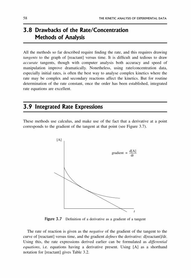
3.8 Drawbacks of the Rate/Concentration
Methods of Analysis
All the methods so far described require finding the rate, and this requires drawing
tangents to the graph of [reactant] versus time. It is difficult and tedious to draw
accurate tangents, though with computer analysis both accuracy and speed of
manipulation improve dramatically. Nonetheless, using rate/concentration data,
especially initial rates, is often the best way to analyse complex kinetics where the
rate may be complex and secondary reactions affect the kinetics. But for routine
determination of the rate constant, once the order has been established, integrated
rate equations are excellent.
3.9 Integrated Rate Expressions
These methods use calculus, and make use of the fact that a derivative at a point
corresponds to the gradient of the tangent at that point (see Figure 3.7).
The rate of reaction is given as the negative of the gradient of the tangent to the
curve of [reactant] versus time, and the gradient defines the derivative: d[reactant]/dt.
Using this, the rate expressions derived earlier can be formulated as differential
equations, i.e. equations having a derivative present. Using [A] as a shorthand
notation for [reactant] gives Table 3.2.
[A]
gradient = d[A]dt
t
Figure 3.7 Definition of a derivative as a gradient of a tangent
58 THE KINETIC ANALYSIS OF EXPERIMENTAL DATA
Differential equations can be solved by integration, and this results in linear
equations relating [reactant] and time, so that the order and rate constant can be found
directly from linear plots.
In scientific work it is always much easier and more accurate to work with linear
relationships. These have an easily defined gradient, and the intercept is accurately
determinable. Also, it is much simpler to discriminate between systematic scatter and
random scatter using linear plots rather than curves.
Integrated rate expressions can also be used to demonstrate that the half-life of a
reaction varies systematically with [reactant], and so is diagnostic of the reaction
order.
3.9.1 Half-lives
The half-life is the time taken for a given concentration to decrease to half of its value;
e.g, if [M]¼ 12 10�3 mol dm�3 at the start of the reaction, then the first half-life is
the time taken for [M] to drop to 6 10�3 mol dm�3; the second half-life is the time
taken for [M] to drop from 6 10�3 mol dm�3 to 3 10�3 mol dm�3; the third half-
life is the time taken for [M] to drop from 3 10�3 mol dm�3 to 1.5 10�3 mol
dm�3; and so on.
Worked Problem 3.7
Question. Draw graphs of [reactant] versus time for the following reactions. Find
as many half-lives as possible, and state the dependence on concentration for each
reaction.
Reaction A
102cmol dm�3 1:000 0:840 0:724 0:506 0:390 0:335 0:225 0:180 0:145
timemin
0 20 40 100 150 200 350 450 600
Table 3.2 Differential rate equations
First order: rate¼ k[A] or �d[A]/dt¼ k[A]
Second order: rate¼ k[A]2 or �d[A]/dt¼ k[A]2
Zero order: rate¼ k[A]0¼ k or �d[A]/dt¼ k [A]0¼ k
3/2 order: rate¼ k[A]3/2 or –d[A]/dt¼ k[A]3/2
INTEGRATED RATE EXPRESSIONS 59
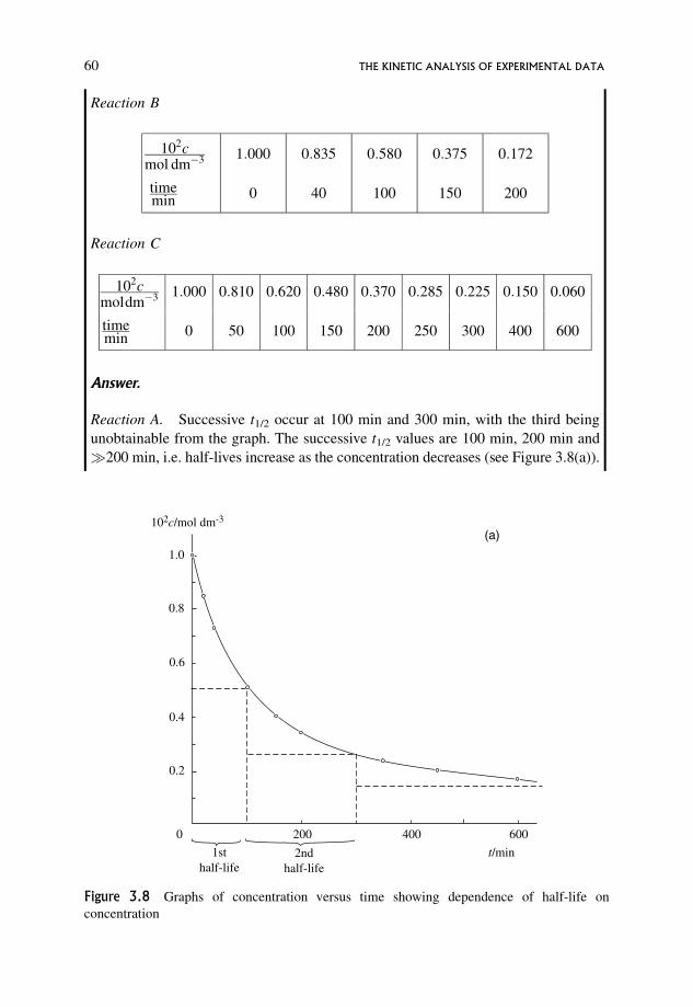
Reaction B
102cmol dm�3 1:000 0:835 0:580 0:375 0:172
timemin
0 40 100 150 200
Reaction C
102cmoldm�3 1:000 0:810 0:620 0:480 0:370 0:285 0:225 0:150 0:060
timemin
0 50 100 150 200 250 300 400 600
Answer.
Reaction A. Successive t1/2 occur at 100 min and 300 min, with the third being
unobtainable from the graph. The successive t1/2 values are 100 min, 200 min and
�200 min, i.e. half-lives increase as the concentration decreases (see Figure 3.8(a)).
1sthalf-life
2ndhalf-life
t/min
1.0
0.8
0.6
0.4
0.2
0 200 400 600
102c/mol dm-3
(a)
Figure 3.8 Graphs of concentration versus time showing dependence of half-life on
concentration
60 THE KINETIC ANALYSIS OF EXPERIMENTAL DATA
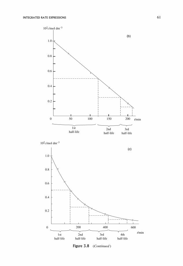
1.0
0.8
0.6
0.4
0.2
0 50 100 150 200
1st half-life
2nd half-life
3rdhalf-life
102c/mol dm_3
t/min
(b)
1.0
0.8
0.6
0.4
0.2
0 200
1sthalf-life
2ndhalf-life
3rdhalf-life
4thhalf-life
400 600
t/min
102c/mol dm_3
(c)
Figure 3.8 (Continued )
INTEGRATED RATE EXPRESSIONS 61
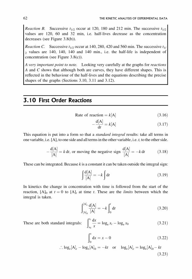
Reaction B. Successive t1/2 occur at 120, 180 and 212 min. The successive t1/2
values are 120, 60 and 32 min, i.e. half-lives decrease as the concentration
decreases (see Figure 3.8(b)).
Reaction C. Successive t1/2 occur at 140, 280, 420 and 560 min. The successive t1/
2 values are 140, 140, 140 and 140 min., i.e. the half-life is independent of
concentration (see Figure 3.8(c)).
A very important point to note. Looking very carefully at the graphs for reactions
A and C shows that although both are curves, they have different shapes. This is
reflected in the behaviour of the half-lives and the equations describing the precise
shapes of the graphs (Sections 3.10, 3.11 and 3.12).
3.10 First Order Reactions
Rate of reaction ¼ k½A ð3:16Þ
� d½Adt¼ k½A ð3:17Þ
This equation is put into a form so that a standard integral results: take all terms in
one variable, i.e. [A], to one side and all terms in the other variable, i.e. t, to the other side.
� d½A½A ¼ k dt; or moving the negative sign
d½A½A ¼ �k dt ð3:18Þ
These can be integrated. Because k is a constant it can be taken outside the integral sign:ðd½A½A ¼ �k
ðdt ð3:19Þ
In kinetics the change in concentration with time is followed from the start of the
reaction, [A]0 at t ¼ 0 to [A]t at time t. These are the limits between which the
integral is taken.
ð½At½A0
d½A½A ¼ �k
ðt
0
dt ð3:20Þ
These are both standard integrals:
ðxt
x0
dx
x¼ loge xt � loge x0 ð3:21Þ
ðx
0
dx ¼ x� 0 ð3:22Þ
; loge½At � loge½A0 ¼ �kt or loge½At ¼ loge½A0� kt
ð3:23Þ
62 THE KINETIC ANALYSIS OF EXPERIMENTAL DATA
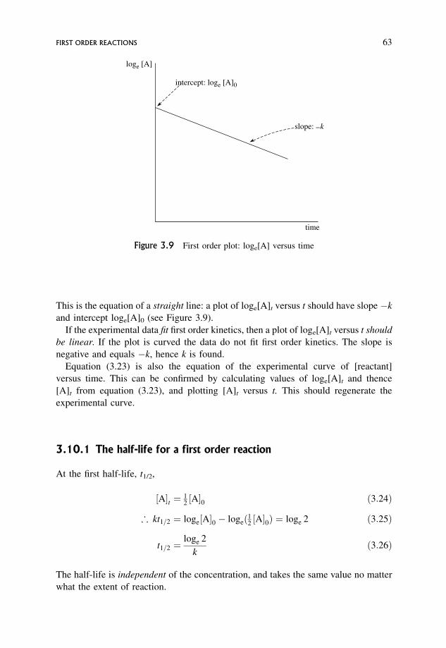
This is the equation of a straight line: a plot of loge[A]t versus t should have slope �k
and intercept loge[A]0 (see Figure 3.9).
If the experimental data fit first order kinetics, then a plot of loge[A]t versus t should
be linear. If the plot is curved the data do not fit first order kinetics. The slope is
negative and equals �k, hence k is found.
Equation (3.23) is also the equation of the experimental curve of [reactant]
versus time. This can be confirmed by calculating values of loge[A]t and thence
[A]t from equation (3.23), and plotting [A]t versus t. This should regenerate the
experimental curve.
3.10.1 The half-life for a first order reaction
At the first half-life, t1/2,
½At ¼ 12½A0 ð3:24Þ
; kt1=2 ¼ loge½A0 � logeð12 ½A0Þ ¼ loge 2 ð3:25Þ
t1=2 ¼loge 2
kð3:26Þ
The half-life is independent of the concentration, and takes the same value no matter
what the extent of reaction.
slope: _k
intercept: loge [A]0
loge [A]
time
Figure 3.9 First order plot: loge[A] versus time
FIRST ORDER REACTIONS 63
Worked Problem 3.8
Question. Show that the decomposition of N2O follows first order kinetics, and
find the rate constant and half-life. Why cannot the methods of Section 3.7 be used
here?
103½N2Omol dm�3 100 61 37 10
time=s 0 50 100 230
Answer. We need to find loge[N2O] to plot loge[N2O]t versus t.
loge½N2Ot �2:30 �2:80 �3:30 �4:61
The graph of loge[N2O]t versus t is linear ; reaction is first order.
Slope¼�1.00 10�2 s�1, hence k¼ 1.00 10�2 s�1.
t1=2 ¼loge 2
1:00 10�2 s�1¼ 69 s:
This value agrees with the value read directly from the experimental graph.
The data is concentration/time data and is immediately adaptable to integrated
rate methods. To use the methods of Section 3.7 the data has to be rate/
concentration data, which is not the manner in which it is presented in this problem.
3.10.2 An extra point about first order reactions
The half-life of a first order reaction remains constant throughout reaction and is
independent of concentration. This applies to any fractional lifetime, though the half-
life is the one most commonly used. The relaxation time is the other common
fractional lifetime. The relaxation time is relevant only to first order reactions, and is
a fractional lifetime which bears a very simple relation to the rate constant as a direct
consequence of the exponential behaviour of first order reactions.
The first order integrated rate equation
loge½At ¼ loge½A0 � kt ð3:23Þ
can also be written in exponential form as
½At ¼ ½A0 expð�ktÞ ð3:27Þ
Fractional lifetimes can be formulated as in Table 3.3.
64 THE KINETIC ANALYSIS OF EXPERIMENTAL DATA
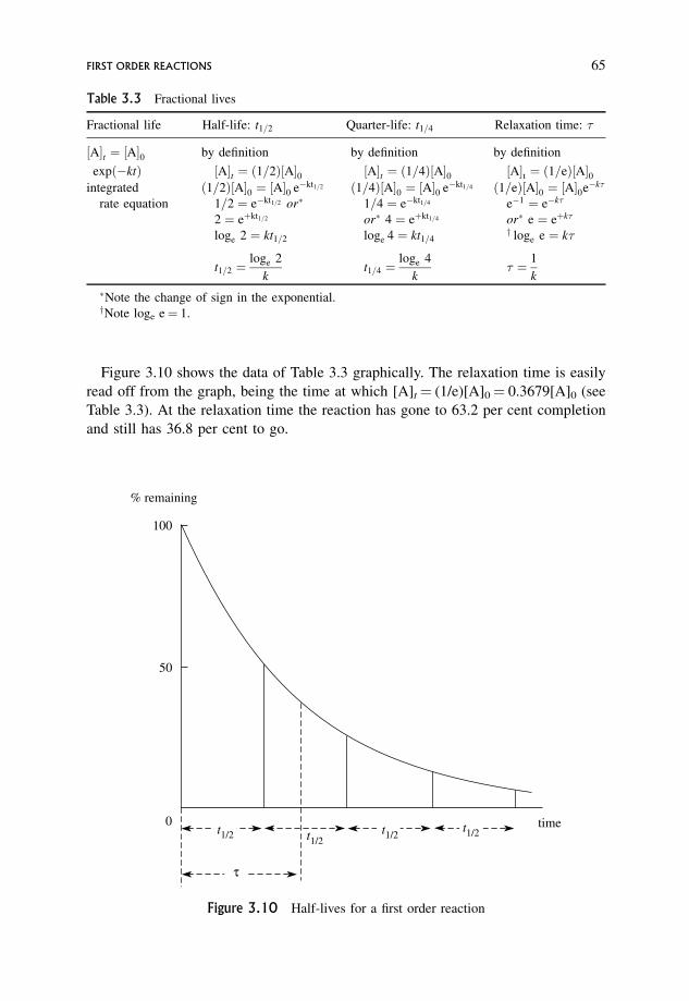
Figure 3.10 shows the data of Table 3.3 graphically. The relaxation time is easily
read off from the graph, being the time at which [A]t¼ (1/e)[A]0¼ 0.3679[A]0 (see
Table 3.3). At the relaxation time the reaction has gone to 63.2 per cent completion
and still has 36.8 per cent to go.
Table 3.3 Fractional lives
Fractional life Half-life: t1=2 Quarter-life: t1=4 Relaxation time: �
½At ¼ ½A0 by definition by definition by definition
expð�ktÞ ½At ¼ ð1=2Þ½A0 ½At ¼ ð1=4Þ½A0 ½At ¼ ð1=eÞ½A0integrated ð1=2Þ½A0 ¼ ½A0 e�kt1=2 ð1=4Þ½A0 ¼ ½A0 e�kt1=4 ð1=eÞ½A0 ¼ ½A0e�k�
rate equation 1=2 ¼ e�kt1=2 or� 1=4 ¼ e�kt1=4 e�1 ¼ e�k�
2 ¼ eþkt1=2 or� 4 ¼ eþkt1=4 or� e ¼ eþk�
loge 2 ¼ kt1=2 loge 4 ¼ kt1=4y loge e ¼ k�
t1=2 ¼loge 2
kt1=4 ¼
loge 4
k� ¼ 1
k
�Note the change of sign in the exponential.yNote loge e¼ 1.
100
50
0 t1/2t1/2t1/2t1/2
τ
% remaining
time
Figure 3.10 Half-lives for a first order reaction
FIRST ORDER REACTIONS 65
Relaxation times become important when studying the approach to equilibrium
either directly or as a result of a small perturbation from equilibrium. They also
emerge directly from ultrasonic relaxation techniques for studying single and multi-
ple equilibria (Section 2.6). However, they only apply to first order or pseudo- first
order processes (Section 3.15).
3.11 Second Order Reactions
Rate of reaction ¼ k½A2 ð3:28Þ
� d½Adt¼ k½A2 ð3:29Þ
Proceeding as before:� d½A½A2¼ k dt or
d½A½A2¼ �k dt ð3:30Þ
Again integrating between the limits [A]0 and [A]t, and t¼ 0 and t, gives
ð½At½A0
d½A½A2¼ �k
ðt
0
dt ð3:31Þ
These are again standard integrals:
ðxt
x0
dx
x2¼ � 1
xt
þ 1
x0
ð3:32Þ
ðx
0
dx ¼ x� 0 ð3:22Þ
; � 1
½Atþ 1
½A0¼ �kt i:e:
1
½At¼ 1
½A0þ kt ð3:33Þ
This is the equation of a straight line: a plot of 1/[A]t versus t should be linear with
slope equal to þk and intercept equal to 1/[A]0 (Figure 3.11).
If the experimental data fit second order kinetics, then a plot of 1/[A]t versus t
should be linear. If the plot is curved, the data do not fit second order kinetics.
The slope is positive and equals þk, hence k is found.
Equation (3.33) is also the equation of the experimental curve of [reactant] versus
time. This can be confirmed by calculating values of 1/[A]t and thence [A]t from
equation (3.33), and plotting [A]t versus t, which should regenerate the experimental
curve.
66 THE KINETIC ANALYSIS OF EXPERIMENTAL DATA

3.11.1 The half-life for a second order reaction
At the first half-life, t1=2; ½At ¼ 12½A0 ð3:24Þ
; kt1=2 ¼1
ð1=2Þ½A0� 1
½A0¼ 1
½A0ð3:34Þ
t1=2 ¼1
k½A0ð3:35Þ
The half-life is proportional to the reciprocal of the concentration, i.e. con-
centration�1, and so the larger the concentration the smaller is the half-life. The
half-life increases as reaction proceeds.
Worked Problem 3.9
Question. Show that the following reaction follows second order kinetics, and
find the rate constant and first half-life.
103½Amol dm�3
7:36 3:68 2:45 1:47 1:23
time=s 0 60 120 240 300
intercept: 1
[A]0
slope: k
time
1[A]
Figure 3.11 Second order plot: 1/[A] versus time
SECOND ORDER REACTIONS 67
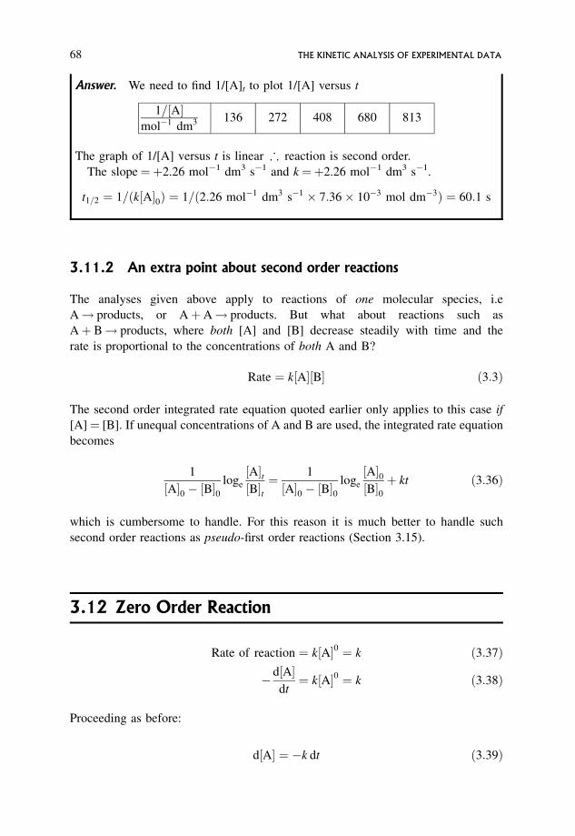
Answer. We need to find 1/[A]t to plot 1/[A] versus t
1=½Amol�1 dm3 136 272 408 680 813
The graph of 1/[A] versus t is linear ; reaction is second order.
The slope¼þ2.26 mol�1 dm3 s�1 and k¼þ2.26 mol�1 dm3 s�1.
t1=2 ¼ 1=ðk½A0Þ ¼ 1=ð2:26 mol�1 dm3 s�1 7:36 10�3 mol dm�3Þ ¼ 60:1 s
3.11.2 An extra point about second order reactions
The analyses given above apply to reactions of one molecular species, i.e
A! products, or AþA! products. But what about reactions such as
Aþ B! products, where both [A] and [B] decrease steadily with time and the
rate is proportional to the concentrations of both A and B?
Rate ¼ k½A½B ð3:3Þ
The second order integrated rate equation quoted earlier only applies to this case if
[A]¼ [B]. If unequal concentrations of A and B are used, the integrated rate equation
becomes
1
½A0 � ½B0loge
½At½Bt¼ 1
½A0 � ½B0loge
½A0½B0þ kt ð3:36Þ
which is cumbersome to handle. For this reason it is much better to handle such
second order reactions as pseudo-first order reactions (Section 3.15).
3.12 Zero Order Reaction
Rate of reaction ¼ k½A0 ¼ k ð3:37Þ
� d½Adt¼ k½A0 ¼ k ð3:38Þ
Proceeding as before:
d½A ¼ �k dt ð3:39Þ
68 THE KINETIC ANALYSIS OF EXPERIMENTAL DATA
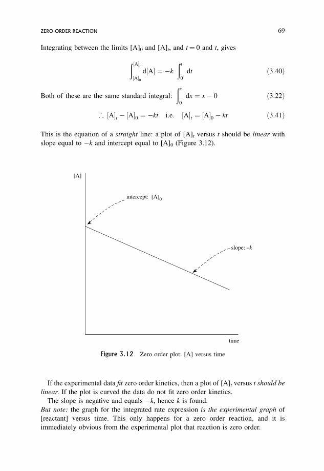
Integrating between the limits [A]0 and [A]t, and t¼ 0 and t, gives
ð½At½A0
d½A ¼ �k
ðt
0
dt ð3:40Þ
Both of these are the same standard integral:
ðx
0
dx ¼ x� 0 ð3:22Þ
; ½At � ½A0 ¼ �kt i:e: ½At ¼ ½A0 � kt ð3:41Þ
This is the equation of a straight line: a plot of [A]t versus t should be linear with
slope equal to �k and intercept equal to [A]0 (Figure 3.12).
If the experimental data fit zero order kinetics, then a plot of [A]t versus t should be
linear. If the plot is curved the data do not fit zero order kinetics.
The slope is negative and equals �k, hence k is found.
But note: the graph for the integrated rate expression is the experimental graph of
[reactant] versus time. This only happens for a zero order reaction, and it is
immediately obvious from the experimental plot that reaction is zero order.
intercept: [A]0
slope: _k
time
[A]
Figure 3.12 Zero order plot: [A] versus time
ZERO ORDER REACTION 69
3.12.1 The half-life for a zero order reaction
At the first half-life, t1=2,
½At ¼ 12½A0 ð3:24Þ
; kt1=2 ¼ ½A0 � 12½A0 ¼ ½A0=2 ð3:42Þ
t1=2 ¼ ½A0=2k ð3:43Þ
The half-life is proportional to the concentration, and so the larger the concentration
the greater is the half-life. The half-life decreases as the reaction proceeds.
Worked Problem 3.10
Question. Show that the following reaction obeys zero order kinetics, and find the
rate constant and first half-life.
102 ½Amol dm�3 13:80 11:05 8:43 5:69 3:00
timeh
0 10 20 30 40
Answer. We need a graph of [A] versus t. This graph is linear, ; reaction is zero
order with slope¼�2.7 10�3 mol dm�3 h�1 and k¼ 2.7 10�3 mol dm�3 h�1.
t1=2 ¼ ½A0=2k ¼ 13:80 10�2 mol dm�3=ð2 2:7 10�3 mol dm�3 h�1Þ ¼ 25:5 h:
The following problem illustrates the use which can be made of half-lives.
Worked Problem 3.11
Question. Look at the answer to problem 3.7 and infer the order of each reaction.
Answer.
Reaction A: half-life increases as concentration decreases, second order.
Reaction B: half-life decreases as concentration decreases, zero order.
Reaction C: half-life remains constant, first order.
70 THE KINETIC ANALYSIS OF EXPERIMENTAL DATA
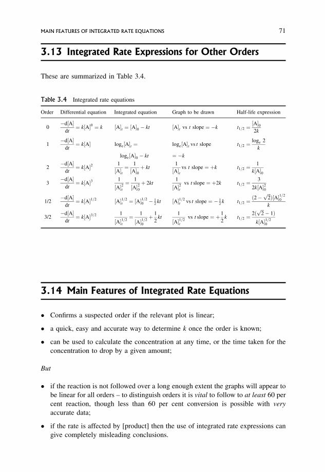
3.13 Integrated Rate Expressions for Other Orders
These are summarized in Table 3.4.
3.14 Main Features of Integrated Rate Equations
� Confirms a suspected order if the relevant plot is linear;
� a quick, easy and accurate way to determine k once the order is known;
� can be used to calculate the concentration at any time, or the time taken for the
concentration to drop by a given amount;
But
� if the reaction is not followed over a long enough extent the graphs will appear to
be linear for all orders – to distinguish orders it is vital to follow to at least 60 per
cent reaction, though less than 60 per cent conversion is possible with very
accurate data;
� if the rate is affected by [product] then the use of integrated rate expressions can
give completely misleading conclusions.
Table 3.4 Integrated rate equations
Order Differential equation Integrated equation Graph to be drawn Half-life expression
0�d½A
dt¼ k½A0 ¼ k ½At ¼ ½A0 � kt ½At vs t slope ¼ �k t1=2 ¼
½A02k
1�d½A
dt¼ k½A loge½At ¼ loge½At vs t slope t1=2 ¼
loge 2
k
loge½A0 � kt ¼ �k
2�d½A
dt¼ k½A2 1
½At¼ 1
½A0þ kt
1
½Atvs t slope ¼ þk t1=2 ¼
1
k½A0
3�d½A
dt¼ k½A3 1
½A2t¼ 1
½A20þ 2kt
1
½A2tvs t slope ¼ þ2k t1=2 ¼
3
2k½A20
1/2�d½A
dt¼ k½A1=2 ½A1=2
t ¼ ½A1=20 � 1
2kt ½A1=2
t vs t slope ¼ � 12
k t1=2 ¼ð2�
ffiffiffi2pÞ½A1=2
0
k
3/2�d½A
dt¼ k½A3=2 1
½A1=2t
¼ 1
½A1=20
þ 1
2kt
1
½A1=2t
vs t slope ¼ þ 1
2k t1=2 ¼
2ðffiffiffi2p� 1Þ
k½A1=20
MAIN FEATURES OF INTEGRATED RATE EQUATIONS 71
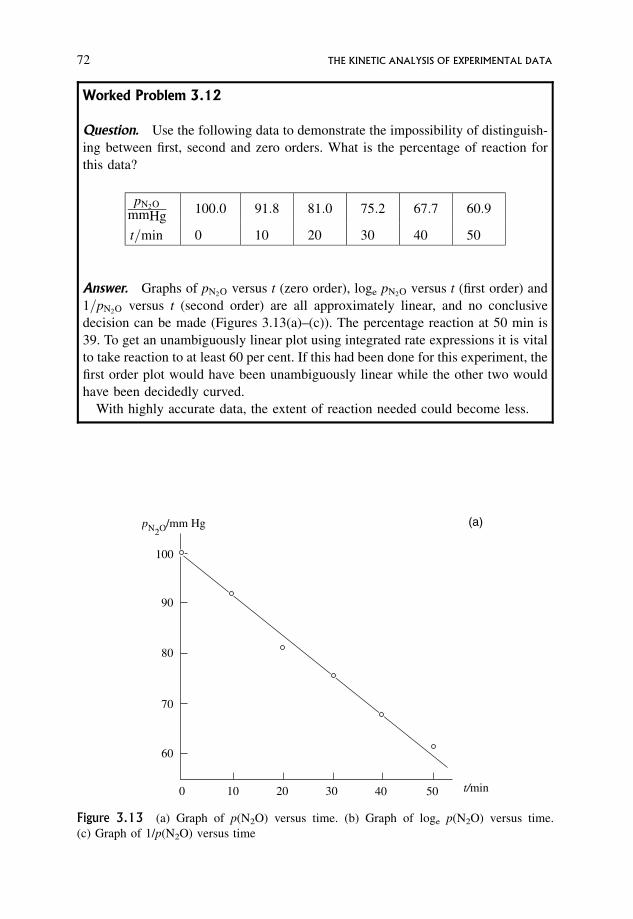
Worked Problem 3.12
Question. Use the following data to demonstrate the impossibility of distinguish-
ing between first, second and zero orders. What is the percentage of reaction for
this data?
pN2O
mmHg100:0 91:8 81:0 75:2 67:7 60:9
t=min 0 10 20 30 40 50
Answer. Graphs of pN2O versus t (zero order), loge pN2O versus t (first order) and
1=pN2O versus t (second order) are all approximately linear, and no conclusive
decision can be made (Figures 3.13(a)–(c)). The percentage reaction at 50 min is
39. To get an unambiguously linear plot using integrated rate expressions it is vital
to take reaction to at least 60 per cent. If this had been done for this experiment, the
first order plot would have been unambiguously linear while the other two would
have been decidedly curved.
With highly accurate data, the extent of reaction needed could become less.
50403020100
60
70
80
90
100
pN2O/mm Hg
t/min
(a)
Figure 3.13 (a) Graph of p(N2O) versus time. (b) Graph of loge p(N2O) versus time.
(c) Graph of 1/p(N2O) versus time
72 THE KINETIC ANALYSIS OF EXPERIMENTAL DATA
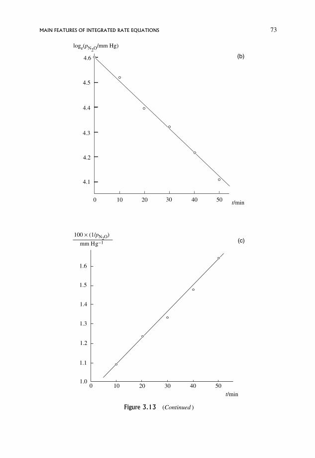
4.6
4.5
4.4
4.3
4.2
4.1
0 10 20 30 40 50 t/min
loge(pN2O/mm Hg)
(b)
1.5
1.4
1.6
(c)
1.3
1.2
1.1
1.00 10 20 30 40 50
t/min
100 × (1/pN2O)
mm Hg_1
Figure 3.13 (Continued )
MAIN FEATURES OF INTEGRATED RATE EQUATIONS 73
3.15 Pseudo-order Reactions
In general, the reaction Aþ B! products has rate equation
Rate ¼ k½A�½B� ð3:44Þ
where � is the order with respect to A and � is the order with respect to B. The total
order is n ¼ �þ �.
Neither (a) the differential method, based on rate/concentration data, nor (b) the
integrated rate method, based on concentration/time data, is easily applicable.
The differential method gives
log rate ¼ log k þ � log½A þ � log½B ð3:45Þ
This is an equation in three unknowns, and the simple log/log plot is no longer
possible.
The integrated rate method has also been shown (Section 3.11.2) to become
cumbersome to use if the reactant concentrations are different.
Trick to overcome this difficulty. If the effect of [B] on the rate is kept constant, i.e.
[B] is kept effectively constant, then the effect of [A] on the rate could be studied
independently of [B], or vice versa. This is attained by keeping one of the
concentrations in large excess over the other throughout the reaction. What does
this mean for the rate equation?
Rate ¼ k½A�½B� ð3:44Þ
If [B] is in excess and effectively constant throughout reaction, then [B]� is also
effectively constant throughout reaction, and can be taken with k to give rate¼ k0 [A]�
where k0 is called the pseudo-rate constant – meaning ‘as if ’.
So, effectively,
rate ¼ k0½A� ð3:46Þwhere
k0 ¼ k½B� ð3:47Þ
and all the previous methods are immediately applicable, and k0 and � can be found.
The value of � can then be found by repeating the experiment with B still in excess,
but at various different values. The value of k0 can be found for each constant excess
[B], giving
k0 ¼ k½B� ð3:47Þlog k0 ¼ log k þ � log½B ð3:48Þ
and so a plot of logk0 versus log[B] should be linear with slope¼ � and inter-
cept¼ log k.
74 THE KINETIC ANALYSIS OF EXPERIMENTAL DATA
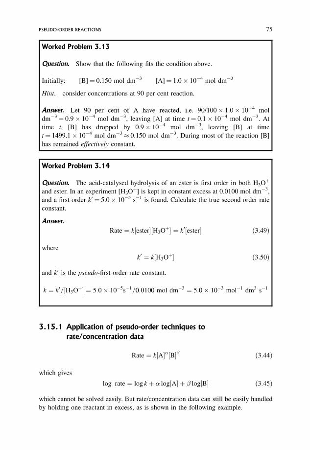
Worked Problem 3.13
Question. Show that the following fits the condition above.
Initially: [B]¼ 0.150 mol dm�3 [A]¼ 1.0 10�4 mol dm�3
Hint. consider concentrations at 90 per cent reaction.
Answer. Let 90 per cent of A have reacted, i.e. 90/100 1.0 10�4 mol
dm�3¼ 0.9 10�4 mol dm�3, leaving [A] at time t¼ 0.1 10�4 mol dm�3. At
time t, [B] has dropped by 0.9 10�4 mol dm�3, leaving [B] at time
t¼ 1499.1 10�4 mol dm�3� 0.150 mol dm�3. During most of the reaction [B]
has remained effectively constant.
Worked Problem 3.14
Question. The acid-catalysed hydrolysis of an ester is first order in both H3Oþ
and ester. In an experiment [H3Oþ] is kept in constant excess at 0.0100 mol dm�3,
and a first order k0 ¼ 5.0 10�5 s�1 is found. Calculate the true second order rate
constant.
Answer.
Rate ¼ k½ester½H3Oþ ¼ k0½ester ð3:49Þ
where
k0 ¼ k½H3Oþ ð3:50Þ
and k0 is the pseudo-first order rate constant.
k ¼ k0=½H3Oþ ¼ 5:0 10�5s�1=0:0100 mol dm�3 ¼ 5:0 10�3 mol�1 dm3 s�1
3.15.1 Application of pseudo-order techniques to
rate/concentration data
Rate ¼ k½A�½B� ð3:44Þ
which gives
log rate ¼ log k þ � log½A þ � log½B ð3:45Þ
which cannot be solved easily. But rate/concentration data can still be easily handled
by holding one reactant in excess, as is shown in the following example.
PSEUDO-ORDER REACTIONS 75
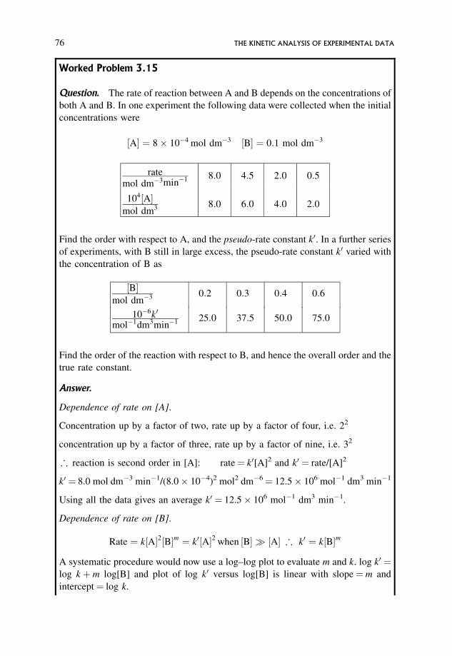
Worked Problem 3.15
Question. The rate of reaction between A and B depends on the concentrations of
both A and B. In one experiment the following data were collected when the initial
concentrations were
½A ¼ 8 10�4 mol dm�3 ½B ¼ 0:1 mol dm�3
ratemol dm�3min�1 8:0 4:5 2:0 0:5
104½Amol dm3 8:0 6:0 4:0 2:0
Find the order with respect to A, and the pseudo-rate constant k0. In a further series
of experiments, with B still in large excess, the pseudo-rate constant k0 varied with
the concentration of B as
½Bmol dm�3 0:2 0:3 0:4 0:6
10�6k0
mol�1dm3min�1 25:0 37:5 50:0 75:0
Find the order of the reaction with respect to B, and hence the overall order and the
true rate constant.
Answer.
Dependence of rate on [A].
Concentration up by a factor of two, rate up by a factor of four, i.e. 22
concentration up by a factor of three, rate up by a factor of nine, i.e. 32
; reaction is second order in [A]: rate¼ k0[A]2 and k0 ¼ rate/[A]2
k0 ¼ 8.0 mol dm�3 min�1/(8.0 10�4)2 mol2 dm�6¼ 12.5 106 mol�1 dm3 min�1
Using all the data gives an average k0 ¼ 12.5 106 mol�1 dm3 min�1.
Dependence of rate on [B].
Rate ¼ k½A2½Bm ¼ k0½A2 when ½B � ½A ; k0 ¼ k½Bm
A systematic procedure would now use a log–log plot to evaluate m and k. log k0 ¼log kþm log[B] and plot of log k0 versus log[B] is linear with slope¼m and
intercept¼ log k.
76 THE KINETIC ANALYSIS OF EXPERIMENTAL DATA
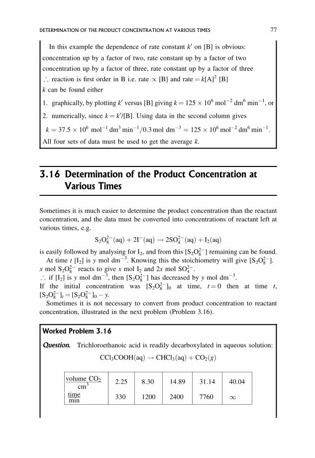
In this example the dependence of rate constant k0 on [B] is obvious:
concentration up by a factor of two, rate constant up by a factor of two
concentration up by a factor of three, rate constant up by a factor of three
; reaction is first order in B i.e. rate / [B] and rate¼ k[A]2 [B]
k can be found either
1. graphically, by plotting k0 versus [B] giving k¼ 125 106 mol�2 dm6 min�1, or
2. numerically, since k¼ k0/[B]. Using data in the second column gives
k ¼ 37:5 106 mol�1 dm3 min�1=0:3 mol dm�3 ¼ 125 106 mol�2 dm6 min�1:
All four sets of data must be used to get the average k.
3.16 Determination of the Product Concentration at
Various Times
Sometimes it is much easier to determine the product concentration than the reactant
concentration, and the data must be converted into concentrations of reactant left at
various times, e.g.
S2O2�8 ðaqÞ þ 2I�ðaqÞ ! 2SO2�
4 ðaqÞ þ I2ðaqÞis easily followed by analysing for I2, and from this [S2O2�
8 ] remaining can be found.
At time t [I2] is y mol dm�3. Knowing this the stoichiometry will give [S2O2�8 ].
x mol S2O2�8 reacts to give x mol I2 and 2x mol SO2�
4 .
; if [I2] is y mol dm�3, then [S2O2�8 ] has decreased by y mol dm�3.
If the initial concentration was [S2O2�8 ]0 at time, t¼ 0 then at time t,
[S2O2�8 ]t¼ [S2O2�
8 ]0� y.
Sometimes it is not necessary to convert from product concentration to reactant
concentration, illustrated in the next problem (Problem 3.16).
Worked Problem 3.16
Question. Trichloroethanoic acid is readily decarboxylated in aqueous solution:
CCl3COOHðaqÞ ! CHCl3ðaqÞ þ CO2ðgÞ
volume CO2
cm3 2:25 8:30 14:89 31:14 40:04
timemin
330 1200 2400 7760 1
DETERMINATION OF THE PRODUCT CONCENTRATION AT VARIOUS TIMES 77

Show the reaction to be first order, and calculate the time taken for the initial
concentration of CCl3COOH to fall by 25 per cent.
Answer.
Volume of CO2 produced when reaction is complete / [CCl3COOH]0
Volume of CO2 produced at time t/ [CCl3COOH]reacted
[CCl3COOH] left at time t¼ [CCl3COOH]0� [CCl3COOH]reacted
/ v1 � vt
where v is the appropriate volume of CO2.
First order plot: loge[A]t¼ loge[A]0� kt.
The decrease in concentration of reactant/ volume of CO2 evolved¼ constant vol.
Hence plot loge(v1 � vt) versus t.
vt
cm3 2:25 8:30 14:89 31:14 40:04
v1 � vt
cm3 37:79 31:74 25:15 8:90 0
logeðv1 � vtÞ 3:632 3:458 3:225 2:186 --
timemin
330 1200 2400 7760 1
Plot of loge(40.04� vt) versus t is linear and reaction is first order.
Slope ¼ �1:94 10�4 min�1;k ¼ 1:94 10�4 min�1
When 25 per cent of the CCl3COOH has reacted, 25 per cent of the final amount of
CO2 will have been formed, i.e. 10.01 cm3.
; at this time [CCl3COOH] / (40.04� 10.01) cm3.
logeð40:04� 10:01Þ ¼ loge 40:04� 1:94 10�4 t
t¼ 1485 min.
Worked Problem 3.17
Question. Why is it possible in this case that the actual concentrations of
CCl3COOH are not needed for the first order plot?
Answer. A logarithm has to be plotted against time and, since loge conc.¼ loge
constantþ loge vol., then a plot of loge vol. will be displaced up or down vertically
78 THE KINETIC ANALYSIS OF EXPERIMENTAL DATA

from the loge conc. by a constant amount equal to loge constant. However, the
slopes of the two graphs will be the same. Hence for a first order plot there is no
need to obtain actual concentrations; a plot of the logarithm of a quantity
proportional to the concentration will suffice. This has considerable value when
physical methods of following reactions are being used.
3.17 Expressing the Rate in Terms of Reactants or
Products for Non-simple Stoichiometry
� Reaction: A! 2B
x mol of A gives 2x mol of B
; rate of production of B is twice that of removal of A
i:e: þ d½B=dt ¼ �2d½A=dt ð3:51Þ
�d½A=dt ¼ þ 12
d½B=dt ð3:52Þ
� Reaction: Aþ 2B! 2CþD
x mol of A reacts with 2x mol of B to give 2x mol of C and x mol of D,
; rate of removal of B is twice that of removal of A, and is twice the rate of
production of D, but equal to the rate of production of C, or rate of removal of A
is half the rate of removal of B, and rate of removal of A is half the rate of
production of C and equal to the rate of production of D.
�2 d½A=dt ¼ �d½B=dt ¼ þd½C=dt ¼ þ2 d½D=dt ð3:53Þ
�d½A=dt ¼ � 12
d½B=dt ¼ þ 12
d½C=dt ¼ þd½D=dt ð3:54Þ
3.18 The Kinetic Analysis for Complex Reactions
Only a relatively few kinetic schemes for complex reactions have differential rate
expressions which can be integrated straightforwardly. Examples are the following.
� A�!k1P1
A�!k2P2
THE KINETIC ANALYSIS FOR COMPLEX REACTIONS 79
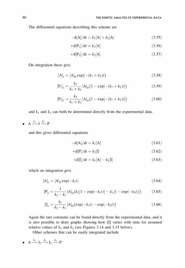
The differential equations describing this scheme are
�d½A=dt ¼ k1½A þ k2½A ð3:55Þ
þd½P1=dt ¼ k1½A ð3:56Þ
þd½P2=dt ¼ k2½A ð3:57Þ
On integration these give
½At ¼ ½A0 expf�ðk1 þ k2Þtg ð3:58Þ
½P1t ¼k1
k1 þ k2
½A0f1� exp½�ðk1 þ k2Þtg ð3:59Þ
½P2t ¼k2
k1 þ k2
½A0f1� exp½�ðk1 þ k2Þtg ð3:60Þ
and k1 and k2 can both be determined directly from the experimental data.
� A�!k1I�!k2
P
and this gives differential equations
�d½A=dt ¼ k1½A ð3:61Þ
þd½P=dt ¼ k2½I ð3:62Þ
þd½I=dt ¼ k1½A � k2½I ð3:63Þ
which on integration give
½At ¼ ½A0 expð�k1tÞ ð3:64Þ
½Pt ¼1
k2 � k1
½A0fk2½1� expð�k1tÞ � k1½1� expð�k2tÞg ð3:65Þ
½It ¼k1
k2 � k1
½A0fexpð�k1tÞ � expð�k2tÞg ð3:66Þ
Again the rate constants can be found directly from the experimental data, and it
is also possible to draw graphs showing how [I] varies with time for assumed
relative values of k1 and k2 (see Figures 3.14 and 3.15 below).
Other schemes that can be easily integrated include
� A�!k1I1�!
k2I2�!
k3P
80 THE KINETIC ANALYSIS OF EXPERIMENTAL DATA
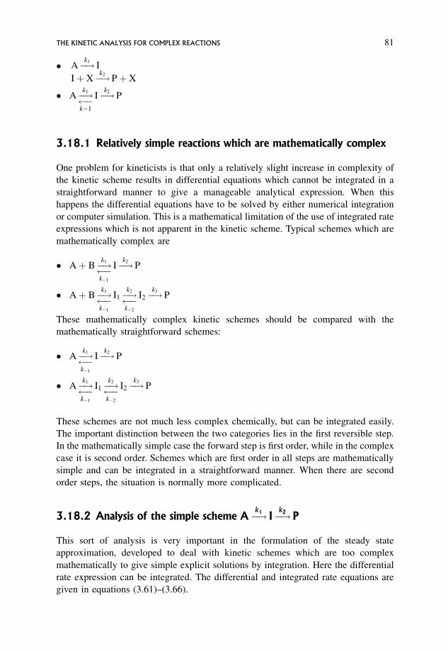
� A�!k1I
Iþ X�!k2Pþ X
� A�!k1
�k�1
I�!k2P
3.18.1 Relatively simple reactions which are mathematically complex
One problem for kineticists is that only a relatively slight increase in complexity of
the kinetic scheme results in differential equations which cannot be integrated in a
straightforward manner to give a manageable analytical expression. When this
happens the differential equations have to be solved by either numerical integration
or computer simulation. This is a mathematical limitation of the use of integrated rate
expressions which is not apparent in the kinetic scheme. Typical schemes which are
mathematically complex are
� Aþ B�!k1
�k�1
I�!k2P
� Aþ B�!k1
�k�1
I1�!k2
�k�2
I2�!k3
P
These mathematically complex kinetic schemes should be compared with the
mathematically straightforward schemes:
� A�!k1
�k�1
I�!k2P
� A�!k1
�k�1
I1�!k2
�k�2
I2�!k3
P
These schemes are not much less complex chemically, but can be integrated easily.
The important distinction between the two categories lies in the first reversible step.
In the mathematically simple case the forward step is first order, while in the complex
case it is second order. Schemes which are first order in all steps are mathematically
simple and can be integrated in a straightforward manner. When there are second
order steps, the situation is normally more complicated.
3.18.2 Analysis of the simple scheme A�!k1 I�!k2 P
This sort of analysis is very important in the formulation of the steady state
approximation, developed to deal with kinetic schemes which are too complex
mathematically to give simple explicit solutions by integration. Here the differential
rate expression can be integrated. The differential and integrated rate equations are
given in equations (3.61)–(3.66).
THE KINETIC ANALYSIS FOR COMPLEX REACTIONS 81
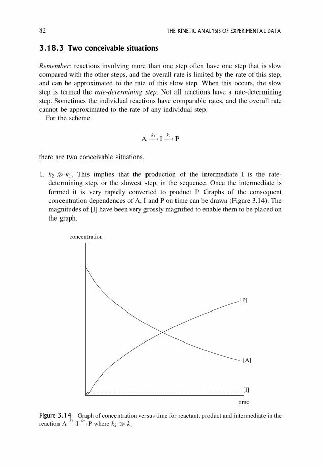
3.18.3 Two conceivable situations
Remember: reactions involving more than one step often have one step that is slow
compared with the other steps, and the overall rate is limited by the rate of this step,
and can be approximated to the rate of this slow step. When this occurs, the slow
step is termed the rate-determining step. Not all reactions have a rate-determining
step. Sometimes the individual reactions have comparable rates, and the overall rate
cannot be approximated to the rate of any individual step.
For the scheme
A�!k1I�!k2
P
there are two conceivable situations.
1. k2 � k1. This implies that the production of the intermediate I is the rate-
determining step, or the slowest step, in the sequence. Once the intermediate is
formed it is very rapidly converted to product P. Graphs of the consequent
concentration dependences of A, I and P on time can be drawn (Figure 3.14). The
magnitudes of [I] have been very grossly magnified to enable them to be placed on
the graph.
time
[I]
[A]
[P]
concentration
Figure 3.14 Graph of concentration versus time for reactant, product and intermediate in the
reaction A�!k1I�!k2
P where k2 � k1
82 THE KINETIC ANALYSIS OF EXPERIMENTAL DATA
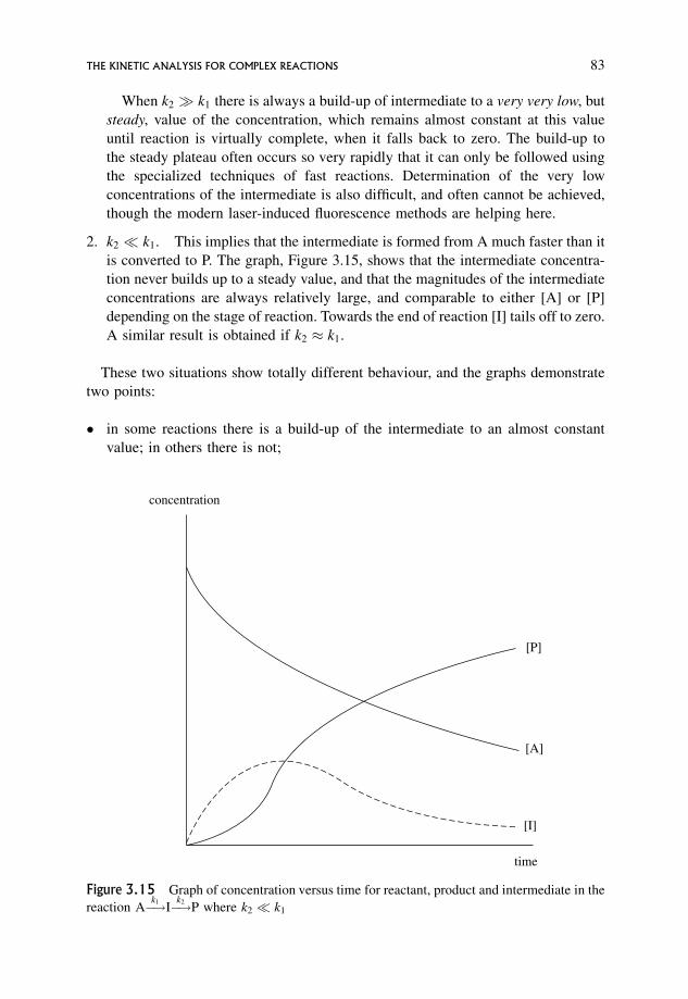
When k2 � k1 there is always a build-up of intermediate to a very very low, but
steady, value of the concentration, which remains almost constant at this value
until reaction is virtually complete, when it falls back to zero. The build-up to
the steady plateau often occurs so very rapidly that it can only be followed using
the specialized techniques of fast reactions. Determination of the very low
concentrations of the intermediate is also difficult, and often cannot be achieved,
though the modern laser-induced fluorescence methods are helping here.
2. k2 � k1. This implies that the intermediate is formed from A much faster than it
is converted to P. The graph, Figure 3.15, shows that the intermediate concentra-
tion never builds up to a steady value, and that the magnitudes of the intermediate
concentrations are always relatively large, and comparable to either [A] or [P]
depending on the stage of reaction. Towards the end of reaction [I] tails off to zero.
A similar result is obtained if k2 � k1.
These two situations show totally different behaviour, and the graphs demonstrate
two points:
� in some reactions there is a build-up of the intermediate to an almost constant
value; in others there is not;
time
concentration
[P]
[A]
[I]
Figure 3.15 Graph of concentration versus time for reactant, product and intermediate in the
reaction A�!k1I�!k2
P where k2 � k1
THE KINETIC ANALYSIS FOR COMPLEX REACTIONS 83
� the criterion for build-up to a plateau is that the intermediate must be present in
very, very low concentrations. This implies that it must always be removed in a
very fast reaction, where in this case k2 � k1. In general the intermediate can be
removed in one reaction, or in a series of reactions, but these must be fast.
3.19 The Steady State Assumption
Reactions involving intermediates present in very very low, and almost constant
concentrations, called steady state concentrations, are in the steady state region. As
will be shown in Chapter 6, many chain and non-chain reactions involve such
intermediates.
If intermediates are present in low steady concentrations this implies that
� the intermediates are very reactive and they never build up to significant
concentrations throughout reaction;
� this, in turn, implies that the total rate of production of the intermediates is
balanced by the total rate of their removal;
� the steady concentration over the time of reaction implies that the rate of change
of the intermediate concentration with time is approximately zero, i.e.
� þd½intermediate=dt � 0 ð3:67Þ
Note: this is written as a rate of formation of the intermediate. This is the normal way
of expressing the change in concentration of the intermediate with time.
� the rate of change of intermediate concentration with time can be expressed in
terms of the rates of all steps producing the intermediate and the rates of all steps
removing the intermediate;
� þd[intermediate]/dt¼ sum of all the rates of production of the intermediate
� sum of all the rates of removal of the intermediate¼ 0
3.19.1 Using this assumption
� This simplifies the subsequent analysis of the kinetic scheme since the relevant
differential equations do not have to be solved. When several intermediates are
present, the steady state treatment is an invaluable aid.
� For given mechanisms, it is possible to predict expressions for the steady state
concentrations of the intermediates in terms of rate constants and reactant
concentrations.
84 THE KINETIC ANALYSIS OF EXPERIMENTAL DATA
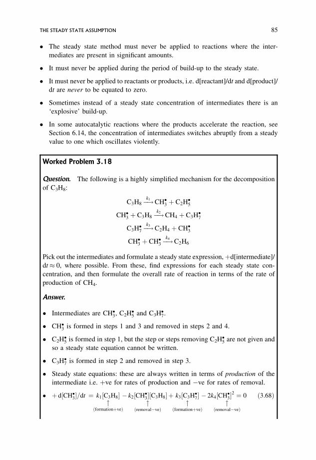
� The steady state method must never be applied to reactions where the inter-
mediates are present in significant amounts.
� It must never be applied during the period of build-up to the steady state.
� It must never be applied to reactants or products, i.e. d[reactant]/dt and d[product]/
dt are never to be equated to zero.
� Sometimes instead of a steady state concentration of intermediates there is an
‘explosive’ build-up.
� In some autocatalytic reactions where the products accelerate the reaction, see
Section 6.14, the concentration of intermediates switches abruptly from a steady
value to one which oscillates violently.
Worked Problem 3.18
Question. The following is a highly simplified mechanism for the decomposition
of C3H8:
C3H8�!k1
CH�3 þ C2H�5
CH�3 þ C3H8�!k2
CH4 þ C3H�7
C3H�7�!k3
C2H4 þ CH�3
CH�3 þ CH�3�!k4
C2H6
Pick out the intermediates and formulate a steady state expression,þd[intermediate]/
dt� 0, where possible. From these, find expressions for each steady state con-
centration, and then formulate the overall rate of reaction in terms of the rate of
production of CH4.
Answer.
� Intermediates are CH�3, C2H�5 and C3H�7.
� CH�3 is formed in steps 1 and 3 and removed in steps 2 and 4.
� C2H�5 is formed in step 1, but the step or steps removing C2H�5 are not given and
so a steady state equation cannot be written.
� C3H�7 is formed in step 2 and removed in step 3.
� Steady state equations: these are always written in terms of production of the
intermediate i.e. þve for rates of production and �ve for rates of removal.
� þ d½CH�3=dt ¼ k1½C3H8"
ðformationþveÞ
� k2½CH�3½C3H8"
ðremoval�veÞ
þ k3½C3H�7"
ðformationþveÞ
� 2k4½CH�32 ¼ 0"
ðremoval�veÞ
ð3:68Þ
THE STEADY STATE ASSUMPTION 85
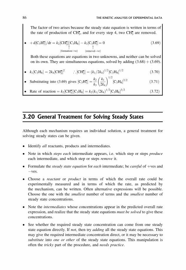
The factor of two arises because the steady state equation is written in terms of
the rate of production of CH�3, and for every step 4, two CH�3 are removed.
� þ d½C3H�7=dt ¼ k2½CH�3½"
ðformationþveÞ
C3H8 � k3½C3H�7"
ðremoval�veÞ
¼ 0 ð3:69Þ
Both these equations are equations in two unknowns, and neither can be solved
on its own. They are simultaneous equations, solved by adding (3.68)þ (3.69).
� k1½C3H8 ¼ 2k4½CH�32 ;½CH�3 ¼ ðk1=2k4Þ1=2½C3H81=2 ð3:70Þ
� Substituting into (3.69) gives ½C3H�7 ¼k2
k3
k1
2k4
� �1=2
½C3H83=2 ð3:71Þ
� Rate of reaction ¼ k2½CH�3½C3H8 ¼ k2ðk1=2k4Þ1=2½C3H83=2 ð3:72Þ
3.20 General Treatment for Solving Steady States
Although each mechanism requires an individual solution, a general treatment for
solving steady states can be given.
� Identify all reactants, products and intermediates.
� Note in which steps each intermediate appears, i.e. which step or steps produce
each intermediate, and which step or steps remove it.
� Formulate the steady state equation for each intermediate; be careful of þves and
�ves.
� Choose a reactant or product in terms of which the overall rate could be
experimentally measured and in terms of which the rate, as predicted by
the mechanism, can be written. Often alternative expressions will be possible.
Choose the one with the smallest number of terms and the smallest number of
steady state concentrations.
� Note the intermediates whose concentrations appear in the predicted overall rate
expression, and realize that the steady state equations must be solved to give these
concentrations.
� See whether the required steady state concentration can come from one steady
state equation directly. If not, then try adding all the steady state equations. This
may give the required intermediate concentration direct, or it may be necessary to
substitute into one or other of the steady state equations. This manipulation is
often the tricky part of the procedure, and needs practice.
86 THE KINETIC ANALYSIS OF EXPERIMENTAL DATA
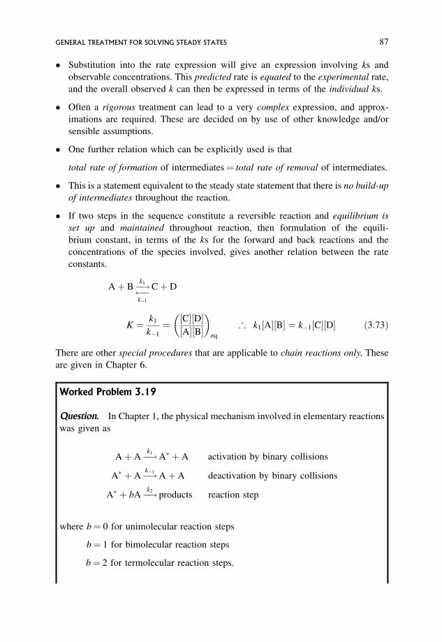
� Substitution into the rate expression will give an expression involving ks and
observable concentrations. This predicted rate is equated to the experimental rate,
and the overall observed k can then be expressed in terms of the individual ks.
� Often a rigorous treatment can lead to a very complex expression, and approx-
imations are required. These are decided on by use of other knowledge and/or
sensible assumptions.
� One further relation which can be explicitly used is that
total rate of formation of intermediates¼ total rate of removal of intermediates.
� This is a statement equivalent to the steady state statement that there is no build-up
of intermediates throughout the reaction.
� If two steps in the sequence constitute a reversible reaction and equilibrium is
set up and maintained throughout reaction, then formulation of the equili-
brium constant, in terms of the ks for the forward and back reactions and the
concentrations of the species involved, gives another relation between the rate
constants.
Aþ B�!k1
�k�1
Cþ D
K ¼ k1
k�1
¼ ½C½D½A½B
� �eq
; k1½A½B ¼ k�1½C½D ð3:73Þ
There are other special procedures that are applicable to chain reactions only. These
are given in Chapter 6.
Worked Problem 3.19
Question. In Chapter 1, the physical mechanism involved in elementary reactions
was given as
Aþ A�!k1A� þ A activation by binary collisions
A� þ A�!k�1Aþ A deactivation by binary collisions
A� þ bA�!k2products reaction step
where b¼ 0 for unimolecular reaction steps
b¼ 1 for bimolecular reaction steps
b¼ 2 for termolecular reaction steps.
GENERAL TREATMENT FOR SOLVING STEADY STATES 87
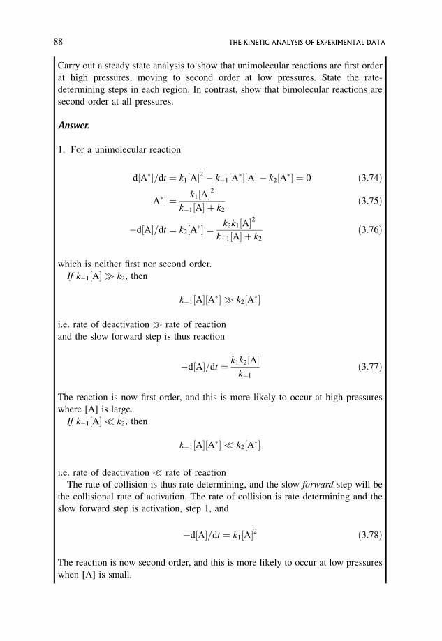
Carry out a steady state analysis to show that unimolecular reactions are first order
at high pressures, moving to second order at low pressures. State the rate-
determining steps in each region. In contrast, show that bimolecular reactions are
second order at all pressures.
Answer.
1. For a unimolecular reaction
d½A�=dt ¼ k1½A2 � k�1½A�½A � k2½A� ¼ 0 ð3:74Þ
½A� ¼ k1½A2
k�1½A þ k2
ð3:75Þ
�d½A=dt ¼ k2½A� ¼k2k1½A2
k�1½A þ k2
ð3:76Þ
which is neither first nor second order.
If k�1½A � k2, then
k�1½A½A� � k2½A�
i.e. rate of deactivation � rate of reaction
and the slow forward step is thus reaction
�d½A=dt ¼ k1k2½Ak�1
ð3:77Þ
The reaction is now first order, and this is more likely to occur at high pressures
where [A] is large.
If k�1½A � k2, then
k�1½A½A� � k2½A�
i.e. rate of deactivation � rate of reaction
The rate of collision is thus rate determining, and the slow forward step will be
the collisional rate of activation. The rate of collision is rate determining and the
slow forward step is activation, step 1, and
�d½A=dt ¼ k1½A2 ð3:78Þ
The reaction is now second order, and this is more likely to occur at low pressures
when [A] is small.
88 THE KINETIC ANALYSIS OF EXPERIMENTAL DATA
2. For a bimolecular reaction
d½A�=dt ¼ k1½A2 � k�1½A�½A � k2½A�½A ¼ 0 ð3:79Þ
½A� ¼ k1½A2
k�1½A þ k2½Að3:80Þ
�d½A=dt ¼ k2½A�½A ¼k2k1½A3
k�1½A þ k2½A¼ k2k1½A2
k�1 þ k2
ð3:81Þ
and this is strictly second order. Nothing can be said about which forward step is
rate determining.
3.21 Reversible Reactions
The simplest example is
A�!k1
�k�1
B
At any time t,
½Atotal ¼ ½Aactual þ ½Bactual ð3:82Þ
During reaction the actual concentrations of A and B are constantly changing, but the
above relation always holds.
When reaction reaches equilibrium, [A]actual and [B]actual remain constant with
time and
K ¼ k1
k�1
¼ ½B½A
� �eq
ð3:83Þ
Worked Problem 3.20
Question. Why is the situation at equilibrium, where �d½Aeq=dt ¼ 0, not a
steady state?
Answer. In the steady state þd[intermediate]/dt¼ 0. The above equilibrium
situation is not a steady state because the concentrations at equilibrium are
significant and are not the very, very low concentrations of the steady state.
REVERSIBLE REACTIONS 89
If reaction is followed by measuring the change in the concentration of A with time:
�d½Aactual=dt ¼ k1½Aactual � k�1½Bactual ð3:84Þ¼ k1½Aactual � k�1f½Atotal � ½Aactualg ð3:85Þ¼ ðk1 þ k�1Þ½Aactual � k�1½Atotal ð3:86Þ
Following standard integration procedures we end up with a non-standard integral,
but this can be overcome by using the properties of the equilibrium position.
At equilibrium the actual concentrations of A and B are constant:
i:e:� d½Aeq=dt ¼ 0 ð3:87Þ
and so at equilibrium and only at equilibrium
�d½Aeq=dt ¼ ðk1 þ k�1Þ½Aactual � k�1½Atotal ¼ 0 ð3:88Þ; k�1½Atotal ¼ ðk1 þ k�1Þ½Aactual; with ½Aactual ¼ ½Aeq ð3:89Þ
Be careful: remember that this equation is only valid at equilibrium.
Substitution for k�1[A]total into equation (3.86) gives
�d½Aactual=dt ¼ ðk1 þ k�1Þf½Aactual � ½Aeqg ð3:90Þ
This equation holds for all situations, not just for equilibrium, and can be integrated
to give
logef½Aactual � ½Aeqg ¼ logef½A0 � ½Aeqg � ðk1 þ k�1Þt ð3:91Þ
This is a first order integrated rate equation and a plot of loge{[A]actual� [A]eq}
versus t has slope¼�(k1þ k�1) and intercept¼ loge{[A]0� [A]eq}
; kobs ¼ k1 þ k�1 ð3:92Þ
and
K ¼ k1=k�1 ð3:93Þ
and so k1 and k�1 can be found.
3.21.1 Extension to other equilibria
When this treatment is extended to other equilibria, non-standard integrals result and
simple integrated rate expressions cannot be obtained. All these equilibria are non-
first order in at least one direction, and all show complex kinetics at all stages away
from the position of equilibrium. However, each one simulates first order behaviour
close to the position of equilibrium, and so is well suited to being studied by single
impulse techniques. Here the equilibrium is slightly displaced and the return to
equilibrium is studied. The term describing such methods is ‘the approach to
equilibrium’. Generalizations of Equation (3.91) can be given
90 THE KINETIC ANALYSIS OF EXPERIMENTAL DATA
Worked Problem 3.21
Question. The isomerization of cis- and trans- 1-ethyl-2-methyl cyclopropane
comes to equilibrium.
cis�!k1
�k�1
trans
At 425.6 �C [trans]eq/[cis]eq¼ 2.79.
Throughout reaction the following data were obtained:
½cismol dm�3 0:016 79 0:014 06 0:011 02 0:008 92 0:007 75
times 0 400 1000 1600 2100
Find k1 and k�1.
Answer. This reaction is one where both the forward and back reactions are first
order. Equation (3.91) can be used.
At all times: [cis]0¼ [cis]actualþ [trans]actual¼ 0.016 79 mol dm�3
At equilibrium: [trans]eq¼ 2.79[cis]eq
; 3:79 ½ciseq ¼ 0:016 79 mol dm�3 ; ½ciseq ¼ 4:43 10�3 mol dm�3
½cistmol dm�3 0:016 79 0:014 06 0:011 02 0:008 92 0:007 75
½cist � ½ciseq
mol dm�3
� �0:012 36 0:009 63 0:006 59 0:004 49 0:003 32
logef½cist � ½ciseqg �4:393 �4:643 �5:022 �5:406 �5:708
times 0 400 1000 1600 2100
A plot of loge{[cis]t� [cis]eq} versus time is linear with slope¼�6.25 10�4 s�1
; k1 þ k�1 ¼ 6:25 10�4 s�1 K ¼ k1=k�1 ¼ 2:79
giving k1 ¼ 4:60 10�4 s�1 and k�1 ¼ 1:65 10�4 s�1
REVERSIBLE REACTIONS 91
3.22 Pre-equilibria
These involve a reversible reaction followed by one or more other reactions. Analysis
shows that if the equilibrium is not established very rapidly then the kinetics are
complex and are not of simple order. Special computer techniques are required to
analyse the results.
If the equilibrium is established very rapidly and is maintained throughout reaction,
analysis becomes straightforward. This can be illustrated by the reaction
A�!k1
�k�1
B�!k2C
Under these conditions
� the step B�!k2C will be rate determining, and the reaction reduces effectively to
B! C;
� so that the mechanistic rate ¼ k2½Bactual; ð3:94Þ
� mathematical analysis shows that for the step B�!k2C to be slow in comparison to
the fast steps A�!k1B and B!k�1
A it is sufficient that k1 or k�1 is large and
k1 þ k�1 � k2;
� although the equilibrium is maintained throughout the reaction both [A]actual and
[B]actual are varying, but the ratio
½Bactual at time t
½Aactual at time t¼ constant ¼ K ð3:95Þ
� the above holds for most reactions studied. If the pre-equilibrium is not set up fast
and maintained, special techniques of analysis are required.
Reactions involving pre-equilibria are discussed in Chapter 8.
3.23 Dependence of Rate on Temperature
Most reactions show an increase in rate as the temperature increases, studied by
measuring the rate constant at various temperatures. Table 3.5 gives rate constants for
bromination of propanone in acidified aqueous Br2 solution.
Table 3.5 shows the dramatic increase in rate constant over a range of a few
degrees. If the rate constant is plotted against temperature an exponential curve is
obtained (Figure 3.16). However, to go further requires data over a much larger range
of temperature.
92 THE KINETIC ANALYSIS OF EXPERIMENTAL DATA
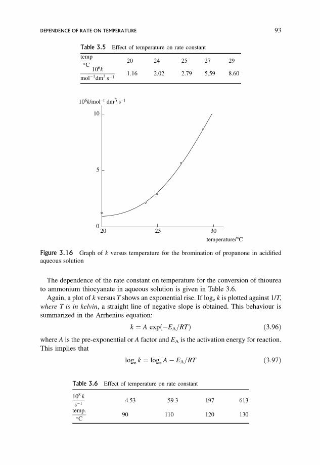
The dependence of the rate constant on temperature for the conversion of thiourea
to ammonium thiocyanate in aqueous solution is given in Table 3.6.
Again, a plot of k versus T shows an exponential rise. If loge k is plotted against 1/T,
where T is in kelvin, a straight line of negative slope is obtained. This behaviour is
summarized in the Arrhenius equation:
k ¼ A expð�EA=RTÞ ð3:96Þ
where A is the pre-exponential or A factor and EA is the activation energy for reaction.
This implies that
loge k ¼ loge A� EA=RT ð3:97Þ
Table 3.6 Effect of temperature on rate constant
108 k
s�14.53 59.3 197 613
temp:�C
90 110 120 130
020 25 30
temperature/°C
106k/mol_1 dm3 s_1
5
10
Figure 3.16 Graph of k versus temperature for the bromination of propanone in acidified
aqueous solution
Table 3.5 Effect of temperature on rate constant
temp�C
20 24 25 27 29
106k
mol�1dm3 s�11.16 2.02 2.79 5.59 8.60
DEPENDENCE OF RATE ON TEMPERATURE 93
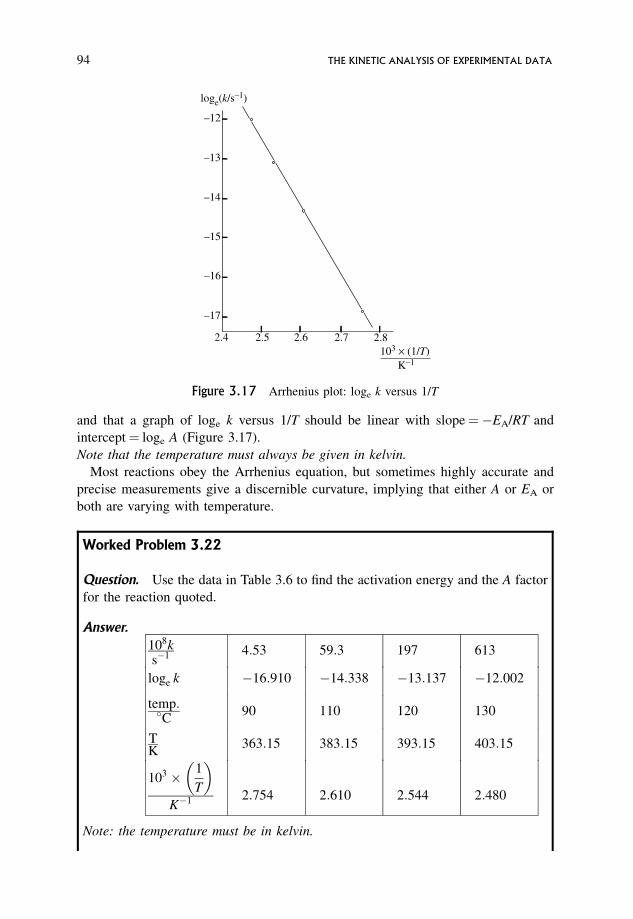
and that a graph of loge k versus 1/T should be linear with slope¼�EA/RT and
intercept¼ loge A (Figure 3.17).
Note that the temperature must always be given in kelvin.
Most reactions obey the Arrhenius equation, but sometimes highly accurate and
precise measurements give a discernible curvature, implying that either A or EA or
both are varying with temperature.
Worked Problem 3.22
Question. Use the data in Table 3.6 to find the activation energy and the A factor
for the reaction quoted.
Answer.108ks�1 4:53 59:3 197 613
loge k �16:910 �14:338 �13:137 �12:002
temp:�C
90 110 120 130
TK
363:15 383:15 393:15 403:15
103 1
T
� �
K�1 2:754 2:610 2:544 2:480
Note: the temperature must be in kelvin.
loge(k/s_1)
_13
_12
_14
_15
_16
_17
2.4 2.5 2.6 2.7 2.8103 × (1/T)
K_1
Figure 3.17 Arrhenius plot: loge k versus 1/T
94 THE KINETIC ANALYSIS OF EXPERIMENTAL DATA
A plot of loge k versus 1/T is linear with slope¼�17.85 103K
; � EA=R ¼ �17:85 103 K and EA ¼ 8:314 17:85 103 J mol�1 K�1 K
¼ 148 kJ mol�1
A has to be found by calculation; extrapolation is impossible. Take one tempera-
ture, its corresponding rate constant and the graphical value of EA, and substitute
into the Arrhenius equation, e.g.
k ¼ 4:53 10�8 s�1 at T ¼ 363:15 K
EA ¼ 148 103 J mol�1 R ¼ 8:314 J mol�1 K�1
4:53 10�8 s�1 ¼ A expð�148 103=8:314 363:15Þ¼ 5:14 10�22 A
A ¼ 8:8 1013 s�1
watch consistency of units: R¼ 8.314 J mol�1 K�1; ; EA must be in J mol�1.
Further reading
Laidler K.J., Chemical Kinetics, 3rd edn, Harper and Row, New York, 1987.
Laidler K.J. and Meiser J.H., Physical Chemistry, 3rd edn, Houghton Mifflin, New
York, 1999.
Alberty R.A. and Silbey R.J., Physical Chemistry, 2nd edn, Wiley, New York, 1996.
Logan S.R., Fundamentals of Chemical Kinetics, Addison-Wesley, Reading, MA,
1996.
�Nicholas J., Chemical Kinetics, Harper and Row, New York, 1976.
�Wilkinson F., Chemical Kinetics and Reaction Mechanisms, Van Nostrand Reinhold,
New York, 1980.�Out of print, but should be in University Libraries.
Further problems
1. (a) The following kinetic data were found for the reaction
A! Bþ C
Expt 1 Expt 2 Expt 3 Expt 4
102½Amol dm�3 0:50 1:78 7:22 19:9
105 ratemol dm�3min�1 0:30 3:80 62:2 475
FURTHER PROBLEMS 95
Explaining your reasoning, find the order of the reaction and hence the rate
constant.
(b) Show that your conclusions are consistent with the following data for the
same reaction at the same temperature.
103½Amol dm�3 10 8:05 6:75 5:0
timemin
0 200 400 800
2. The following data refer to the vapour phase decomposition of ethylene oxide at
414 �C:
C2H4OðgÞ ! CH4ðgÞ þ COðgÞ
timemin
0 9 13 18 50 100
ptotal
mmHg 116:5 129:4 134:7 141:3 172:1 201:2
Find the order and rate constant for this reaction.
What further information would be needed to determine the activation energy?
3. From the following measurements of the initial rates of a reaction involving
reactants A, B and C, estimate the order of reaction with respect to each reactant
and the value of the rate constant. [A]0 etc refer to the initial concentrations.
Expt 1 2 3 4
105 initial ratemol dm�3 s�1 2:5 3:75 10:0 2:5
½A0mol dm�3 0:010 0:010 0:010 0:020
½B0mol dm�3 0:005 0:005 0:010 0:005
½C0mol dm�3 0:010 0:015 0:010 0:010
4. The thermal decomposition of nitryl chloride obeys the stoichiometric equation
2NO2ClðgÞ ! 2NO2ðgÞ þ Cl2ðgÞ
(a) Use the following data to show that the reaction obeys first order
kinetics. Find the time required for the partial pressure of NO2Cl to fall by
96 THE KINETIC ANALYSIS OF EXPERIMENTAL DATA
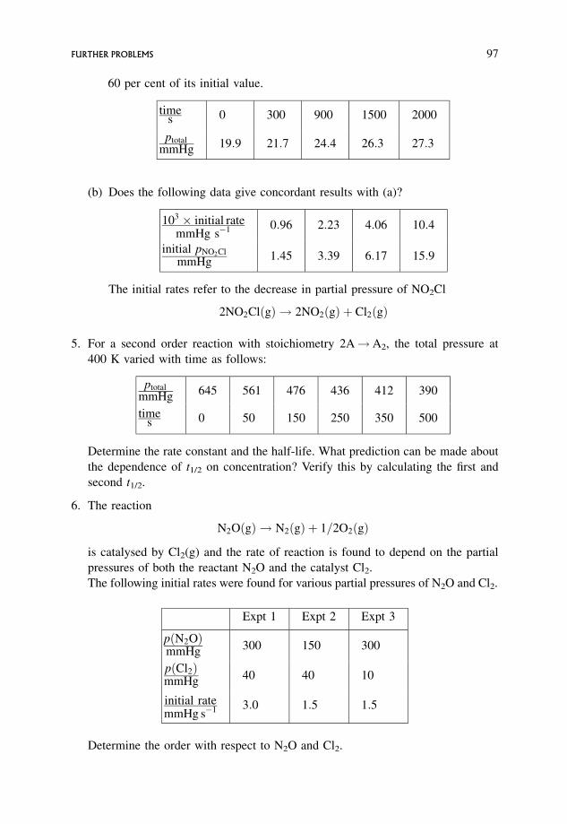
60 per cent of its initial value.
times 0 300 900 1500 2000
ptotalmmHg 19:9 21:7 24:4 26:3 27:3
(b) Does the following data give concordant results with (a)?
103 initial ratemmHg s�1 0:96 2:23 4:06 10:4
initial pNO2Cl
mmHg 1:45 3:39 6:17 15:9
The initial rates refer to the decrease in partial pressure of NO2Cl
2NO2ClðgÞ ! 2NO2ðgÞ þ Cl2ðgÞ
5. For a second order reaction with stoichiometry 2A!A2, the total pressure at
400 K varied with time as follows:
ptotal
mmHg 645 561 476 436 412 390
times 0 50 150 250 350 500
Determine the rate constant and the half-life. What prediction can be made about
the dependence of t1/2 on concentration? Verify this by calculating the first and
second t1/2.
6. The reaction
N2OðgÞ ! N2ðgÞ þ 1=2O2ðgÞ
is catalysed by Cl2(g) and the rate of reaction is found to depend on the partial
pressures of both the reactant N2O and the catalyst Cl2.
The following initial rates were found for various partial pressures of N2O and Cl2.
Expt 1 Expt 2 Expt 3
pðN2OÞmmHg 300 150 300
pðCl2ÞmmHg 40 40 10
initial ratemmHg s�1 3:0 1:5 1:5
Determine the order with respect to N2O and Cl2.
FURTHER PROBLEMS 97
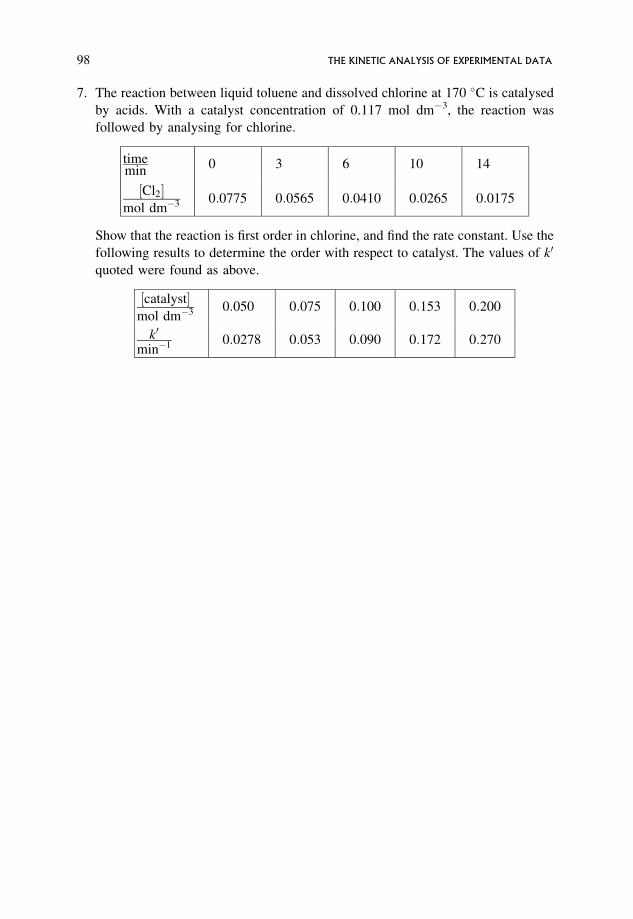
7. The reaction between liquid toluene and dissolved chlorine at 170 �C is catalysed
by acids. With a catalyst concentration of 0.117 mol dm�3, the reaction was
followed by analysing for chlorine.
timemin
0 3 6 10 14
½Cl2mol dm�3 0:0775 0:0565 0:0410 0:0265 0:0175
Show that the reaction is first order in chlorine, and find the rate constant. Use the
following results to determine the order with respect to catalyst. The values of k0
quoted were found as above.
½catalystmol dm�3 0:050 0:075 0:100 0:153 0:200
k0
min�1 0:0278 0:053 0:090 0:172 0:270
98 THE KINETIC ANALYSIS OF EXPERIMENTAL DATA
4 Theories of Chemical
Reactions
Developments in theoretical chemical kinetics have made dramatic progress in the
last few decades and these have been complemented by developments in experi-
mental techniques, particularly molecular beam experiments and modern spectro-
scopic techniques. Many of these advances are modifications and developments of the
original basic theories. It is essential that the concepts behind these older ideas are
fully understood before moving on to the recent ideas.
Aims
By the end of this chapter you should be able to
� understand simple collision theory and be aware of its defects,
� appreciate that molecular beam ideas are much more physically realistic than thoseof simple collision theory,
� have an awareness of the power of modified collision theory,
� list the properties of potential energy surfaces relevant to transition state theory,
� follow an outline of the theoretical derivation of transition state theory inpartition function form, and in thermodynamic form,
� compare predictions of collision theory, transition state theory and experimentand
� understand the fundamental concepts underlying unimolecular theory.
An Introduction to Chemical Kinetics. Margaret Robson Wright# 2004 John Wiley & Sons, Ltd. ISBNs: 0-470-09058-8 (hbk) 0-470-09059-6 (pbk)
4.1 Collision Theory
Simple collision theory assumes reaction occurs when molecules, with energy greater
than a critical minimum, collide. Calculation of two quantities, the total rate of
collision of reactant molecules and the fraction of molecules which have at least the
critical energy, gives an equation to compare with the experimental Arrhenius
equation:k ¼ A expð�EA=RTÞ ð4:1Þ
The main features of collision theory are
� molecules are hard spheres, i.e. there are no inter molecular interactions,
� vibrational and rotational structures of reactants and products are ignored,
� the activated complex plays no part in the theory, and
� redistribution of energy on reaction is ignored.
Molecular beams, chemiluminescence and laser-induced fluorescence experiments show
the theory in its simple form to be fundamentally flawed, with internal states of reactants
and products and the redistribution of energy on reaction being of fundamental importance.
Molecular beam experiments study reactive and non-reactive collisions between
molecules by observing the deflection of each molecule from its original path as a
result of the collision. By studying the amount of scattering into various angles, much
useful kinetic information can be found.
Chemiluminesence is emission of radiation from the products of a chemical
reaction, and is normally associated with exothermic reactions where the products
are in excited vibrational, rotational and sometimes electronic states. The particular
excited states which are produced immediately after reaction has occurred can be
studied and kinetic information obtained. Such studies also throw doubts on the
validity of assuming that these states play no part.
Laser-induced fluorescence has been discussed in Chapter 2. Lasers excite
molecules to excited levels from which they can lose energy by emission of radiation.
This technique has been of major importance in the molecular beam experiments
which force modification of the original collision theory outlined below.
4.1.1 Definition of a collision in simple collision theory
For reaction between unlike molecules, Aþ B! products, only collisions between A
and B can lead to reaction, and the appropriate total rate of collision is for collisions
between A and B only.
Molecules A and B approach with relative velocity vAB, represented as B being
stationary and A approaching with velocity vAB.
A � �!vAB � BðstationaryÞ
100 THEORIES OF CHEMICAL REACTIONS
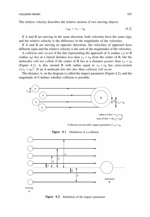
The relative velocity describes the relative motion of two moving objects:
vAB ¼ vA � vB ð4:2Þ
If A and B are moving in the same direction, both velocities have the same sign,
and the relative velocity is the difference in the magnitudes of the velocities.
If A and B are moving in opposite directions, the velocities of approach have
different signs and the relative velocity is the sum of the magnitudes of the velocities.
A collision only occurs if the line representing the approach of A (radius rA) to B
(radius rB) lies at a lateral distance less than rAþ rB from the centre of B, but the
molecules will not collide if the centre of B lies at a distance greater than rAþ rB
(Figure 4.1). A disc around B with radius equal to rAþ rB has cross-section
�ðrA þ rBÞ2. If an A molecule hits this disc then collision will occur.
The distance, b, on the diagram is called the impact parameter (Figure 4.2), and the
magnitude of b defines whether collision is possible.
A
AB
A
A
rΒ
rΑ
rΑ + rΒ
radius of disc = rΑ + rΒarea of disc = π(rΑ + rΒ)2
Collisions are possible: impact parameter ≤ rΑ + rΒ
Figure 4.1 Definition of a collision
movingA
stationaryB
b
b
b
bb
b
Figure 4.2 Definition of the impact parameter
COLLISION THEORY 101
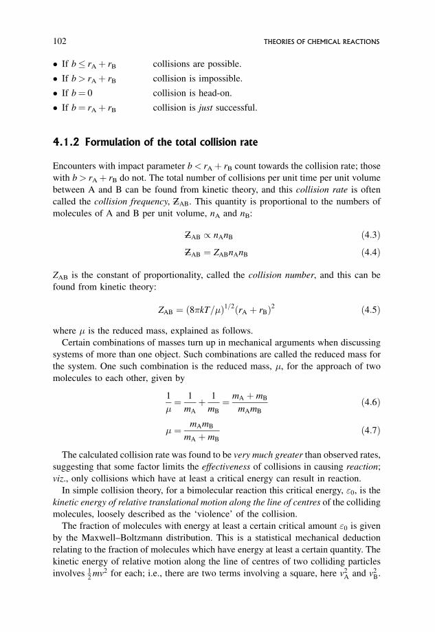
� If b� rAþ rB collisions are possible.
� If b > rAþ rB collision is impossible.
� If b¼ 0 collision is head-on.
� If b¼ rAþ rB collision is just successful.
4.1.2 Formulation of the total collision rate
Encounters with impact parameter b < rAþ rB count towards the collision rate; those
with b > rAþ rB do not. The total number of collisions per unit time per unit volume
between A and B can be found from kinetic theory, and this collision rate is often
called the collision frequency, Z�AB. This quantity is proportional to the numbers of
molecules of A and B per unit volume, nA and nB:
Z�AB / nAnB ð4:3Þ
Z�AB ¼ ZABnAnB ð4:4Þ
ZAB is the constant of proportionality, called the collision number, and this can be
found from kinetic theory:
ZAB ¼ ð8�kT=�Þ1=2ðrA þ rBÞ2 ð4:5Þ
where � is the reduced mass, explained as follows.
Certain combinations of masses turn up in mechanical arguments when discussing
systems of more than one object. Such combinations are called the reduced mass for
the system. One such combination is the reduced mass, �, for the approach of two
molecules to each other, given by
1
�¼ 1
mA
þ 1
mB
¼ mA þ mB
mAmB
ð4:6Þ
� ¼ mAmB
mA þ mB
ð4:7Þ
The calculated collision rate was found to be very much greater than observed rates,
suggesting that some factor limits the effectiveness of collisions in causing reaction;
viz., only collisions which have at least a critical energy can result in reaction.
In simple collision theory, for a bimolecular reaction this critical energy, "0, is the
kinetic energy of relative translational motion along the line of centres of the colliding
molecules, loosely described as the ‘violence’ of the collision.
The fraction of molecules with energy at least a certain critical amount "0 is given
by the Maxwell–Boltzmann distribution. This is a statistical mechanical deduction
relating to the fraction of molecules which have energy at least a certain quantity. The
kinetic energy of relative motion along the line of centres of two colliding particles
involves 12
mv2 for each; i.e., there are two terms involving a square, here v2A and v2
B.
102 THEORIES OF CHEMICAL REACTIONS
This is called an energy in two squared terms. The Maxwell–Boltzmann expression
for such a situation is
n
ntotal
¼ exp�"kT
� �ð4:8Þ
where the fraction refers to the number of molecules with energy at least " in two
squared terms.
In more complex situations, where e.g. rotations and vibrations are involved, there
will be squared terms relating to each rotational and each vibrational mode. Each
rotational mode involves the square of the angular velocity and contributes one
squared term. Each vibrational mode involves a term from the potential energy and a
term for the kinetic energy of vibration, and contributes two squared terms if the
vibration is harmonic. If there are a total of 2s squared terms, then this is called
energy in 2s squared terms. The Maxwell–Boltzmann distribution is correspondingly
more complex (Section 4.5.8).
The fraction of molecules with energy at least "0 along the line of centres is thus a
simple exponential term, expð�"0=kTÞ, so that the total rate of reaction is equal to the
total rate of collisions modified by this exponential energy term. This is the total rate
of successful collisions:
calculated rate of reaction ¼ ZABnAnB expð�"0=kTÞ ð4:9Þ¼ ð8�kT=�Þ1=2ðrA þ rBÞ2nAnB expð�"0=kTÞ ð4:10Þ
This rate of reaction can also be given as kcalcnAnB, giving for the rate constant:
kcalc ¼ ZAB expð�"0=kTÞ ð4:11Þ¼ ð8�kT=�Þ1=2ðrA þ rBÞ2 expð�"0=kTÞ ð4:12Þ
The term in (rAþ rB)2 in ZAB can be replaced by the collision diameter, d2AB, or the
cross sectional area, � ¼ �ðrA þ rBÞ2.
Note. The area of a circle is �r2, and the area of one surface of a disc is also �r2.
These equations, as quoted, are in molecular units, and when comparison is made
with the experimental Arrhenius equation, equation (4.11) must be converted into
molar units.
Conversion to molar units:
� per molecule must be converted to an equivalent quantity per mole;
k in J K�1 must be converted to R in J K�1 mol�1;
"0 in J must be converted into EA in kJ mol�1;
nA and nB, as number of molecules per unit volume, into concentrations in mol dm�3;
or vice versa depending on how the values are given initially.
COLLISION THEORY 103
Worked Problem 4.1
Question. Taking Z, the collision number, to be 4 1010 mol�1 dm3 s�1,
calculate the rate of collision, Z�, for two reactants both at a concentration of
2:5 10�2 mol dm�3. Compare the result with an experimental rate of reaction of
1:4 10�6 mol dm�3 s�1. Suggest a reason for any discrepancy.
Answer.
Rate of collision ¼ Z ½A�½B� ð4:13Þ¼ 4 1010 2:5 10�2 2:5 10�2 mol dm�3 s�1
¼ 2:5 107 mol dm�3 s�1:
Observed rate of reaction ¼ 1:4 10�6 mol dm�3 s�1:
Observed rate=rate of collision ¼ 1:4 10�6 mol dm�3 s�1
2:5 107 mol dm�3 s�1
¼ 5:6 10�14
Observed rate collision rate, suggesting that only a few collisions lead to
reaction.
Problem 4.1 indicates that there is a large factor limiting the effectiveness of
collisions leading to reaction. As shown in Section 4.1.2, this is the requirement for a
certain critical energy, where for bimolecular reactions the activation energy is the
kinetic energy of relative translational motion along the line of centres of the
colliding molecules. When molecules collide they will not react unless this energy
is at least the critical value, the activation energy. The rate of reaction depends
crucially on the magnitude of this activation energy. The Arrhenius equation, (4.1),
can be used to demonstrate the dramatic effect which the magnitude of EA has on the
rate constant and hence on the rate.
Worked Problem 4.2
Question. Use the Arrhenius equation to calculate the rate constants for the
following two reactions which have the same magnitude for the A factor,
A ¼ 5 1010 mol�1 dm3 s�1. The temperature is 300 K.
(a) A reaction with activation energy of þ30 kJ mol�1.
(b) A reaction with activation energy of þ100 kJ mol�1.
Answer.
k ¼ A expð�EA=RTÞ ð4:1Þ
104 THEORIES OF CHEMICAL REACTIONS
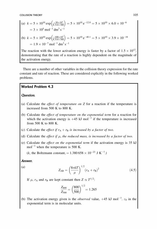
(a) k ¼ 5 1010 exp �30103
8:314300
� �¼ 5 1010 e�12:0 ¼ 5 1010 6:0 10�6
¼ 3 105 mol�1 dm3 s�1
(b) k ¼ 5 1010 exp �100103
8:314300
� �¼ 5 1010 e�40:1 ¼ 5 1010 3:9 10�18
¼ 1:9 10�7 mol�1 dm3 s�1
The reaction with the lower activation energy is faster by a factor of 1:5 1012,
demonstrating that the rate of a reaction is highly dependent on the magnitude of
the activation energy.
There are a number of other variables in the collision theory expression for the rate
constant and rate of reaction. These are considered explicitly in the following worked
problems.
Worked Problem 4.3
Question.
(a) Calculate the effect of temperature on Z for a reaction if the temperature is
increased from 500 K to 800 K.
(b) Calculate the effect of temperature on the exponential term for a reaction for
which the activation energy is þ45 kJ mol�1 if the temperature is increased
from 500 K to 800 K.
(c) Calculate the effect if rA þ rB is increased by a factor of two.
(d) Calculate the effect if �, the reduced mass, is increased by a factor of two.
(e) Calculate the effect on the exponential term if the activation energy is 35 kJ
mol�1 when the temperature is 500 K.
(k, the Boltzmann constant,¼ 1.380 658 10�23 J K�1.)
Answer.
(a)ZAB ¼
8�kT
�
� �1=2
ðrA þ rBÞ2 ð4:5Þ
If �, rA and rB are kept constant then Z / T1=2:
Z800
Z500
¼ 800
500
� �1=2
¼ 1:265
(b) The activation energy given is the observed value, þ45 kJ mol�1. "0 in the
exponential term is in molecular units.
COLLISION THEORY 105
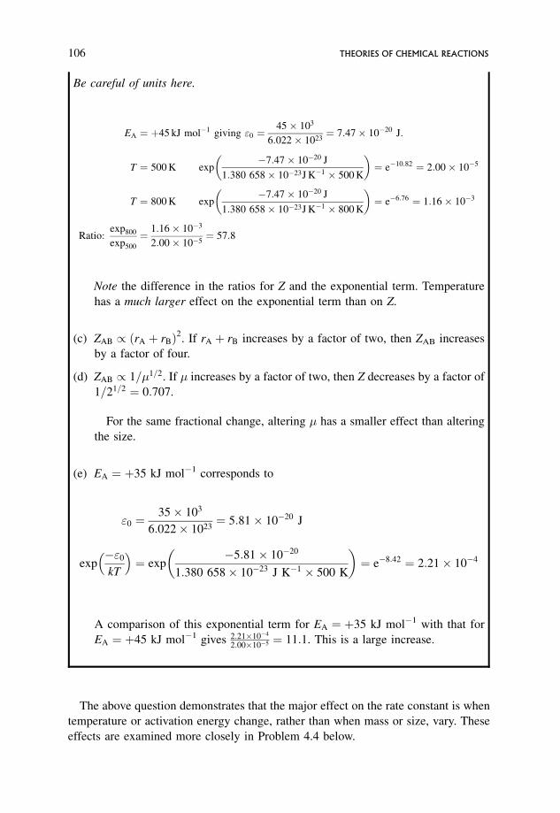
Be careful of units here.
EA ¼ þ45 kJ mol�1 giving "0 ¼45 103
6:022 1023¼ 7:47 10�20 J:
T ¼ 500 K exp�7:47 10�20 J
1:380 658 10�23J K�1 500 K
� �¼ e�10:82 ¼ 2:00 10�5
T ¼ 800 K exp�7:47 10�20 J
1:380 658 10�23J K�1 800 K
� �¼ e�6:76 ¼ 1:16 10�3
Ratio:exp800
exp500
¼ 1:16 10�3
2:00 10�5¼ 57:8
Note the difference in the ratios for Z and the exponential term. Temperature
has a much larger effect on the exponential term than on Z.
(c) ZAB / ðrA þ rBÞ2. If rA þ rB increases by a factor of two, then ZAB increases
by a factor of four.
(d) ZAB / 1=�1=2. If � increases by a factor of two, then Z decreases by a factor of
1=21=2 ¼ 0:707.
For the same fractional change, altering � has a smaller effect than altering
the size.
(e) EA ¼ þ35 kJ mol�1 corresponds to
"0 ¼35 103
6:022 1023¼ 5:81 10�20 J
exp�"0
kT
� �¼ exp
�5:81 10�20
1:380 658 10�23 J K�1 500 K
� �¼ e�8:42 ¼ 2:21 10�4
A comparison of this exponential term for EA ¼ þ35 kJ mol�1 with that for
EA ¼ þ45 kJ mol�1 gives 2:2110�4
2:0010�5 ¼ 11:1. This is a large increase.
The above question demonstrates that the major effect on the rate constant is when
temperature or activation energy change, rather than when mass or size, vary. These
effects are examined more closely in Problem 4.4 below.
106 THEORIES OF CHEMICAL REACTIONS
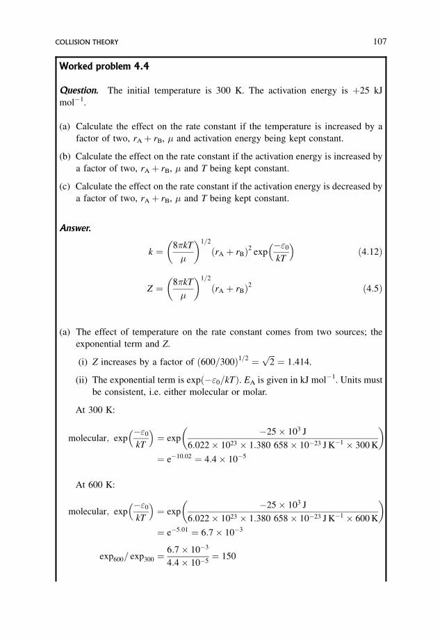
Worked problem 4.4
Question. The initial temperature is 300 K. The activation energy is þ25 kJ
mol�1.
(a) Calculate the effect on the rate constant if the temperature is increased by a
factor of two, rAþ rB, � and activation energy being kept constant.
(b) Calculate the effect on the rate constant if the activation energy is increased by
a factor of two, rAþ rB, � and T being kept constant.
(c) Calculate the effect on the rate constant if the activation energy is decreased by
a factor of two, rAþ rB, � and T being kept constant.
Answer.
k ¼ 8�kT
�
� �1=2
ðrA þ rBÞ2 exp�"0
kT
� �ð4:12Þ
Z ¼ 8�kT
�
� �1=2
ðrA þ rBÞ2 ð4:5Þ
(a) The effect of temperature on the rate constant comes from two sources; the
exponential term and Z.
(i) Z increases by a factor of ð600=300Þ1=2 ¼ffiffiffi2p¼ 1:414.
(ii) The exponential term is exp �"0=kTð Þ. EA is given in kJ mol�1. Units must
be consistent, i.e. either molecular or molar.
At 300 K:
molecular; exp�"0
kT
� �¼ exp
�25 103 J
6:022 1023 1:380 658 10�23 J K�1 300 K
� �
¼ e�10:02 ¼ 4:4 10�5
At 600 K:
molecular; exp�"0
kT
� �¼ exp
�25 103 J
6:022 1023 1:380 658 10�23 J K�1 600 K
� �
¼ e�5:01 ¼ 6:7 10�3
exp600= exp300 ¼6:7 10�3
4:4 10�5¼ 150
COLLISION THEORY 107
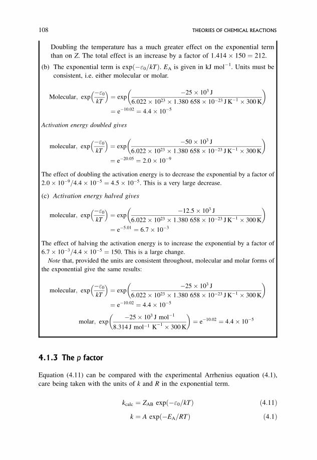
Doubling the temperature has a much greater effect on the exponential term
than on Z. The total effect is an increase by a factor of 1:414 150 ¼ 212.
(b) The exponential term is exp �"0=kTð Þ. EA is given in kJ mol�1. Units must be
consistent, i.e. either molecular or molar.
Molecular; exp�"0
kT
� �¼ exp
�25 103 J
6:022 1023 1:380 658 10�23 J K�1 300 K
� �
¼ e�10:02 ¼ 4:4 10�5
Activation energy doubled gives
molecular; exp�"0
kT
� �¼ exp
�50 103 J
6:022 1023 1:380 658 10�23 J K�1 300 K
� �
¼ e�20:05 ¼ 2:0 10�9
The effect of doubling the activation energy is to decrease the exponential by a factor of
2:0 10�9=4:4 10�5 ¼ 4:5 10�5. This is a very large decrease.
(c) Activation energy halved gives
molecular; exp�"0
kT
� �¼ exp
�12:5 103 J
6:022 1023 1:380 658 10�23 J K�1 300 K
� �
¼ e�5:01 ¼ 6:7 10�3
The effect of halving the activation energy is to increase the exponential by a factor of
6:7 10�3=4:4 10�5 ¼ 150. This is a large change.
Note that, provided the units are consistent throughout, molecular and molar forms of
the exponential give the same results:
molecular; exp�"0
kT
� �¼ exp
�25 103 J
6:022 1023 1:380 658 10�23 J K�1 300 K
� �
¼ e�10:02 ¼ 4:4 10�5
molar; exp�25 103 J mol�1
8:314 J mol�1 K�1 300 K
� �¼ e�10:02 ¼ 4:4 10�5
4.1.3 The p factor
Equation (4.11) can be compared with the experimental Arrhenius equation (4.1),
care being taken with the units of k and R in the exponential term.
kcalc ¼ ZAB expð�"0=kTÞ ð4:11Þ
k ¼ A expð�EA=RTÞ ð4:1Þ
108 THEORIES OF CHEMICAL REACTIONS
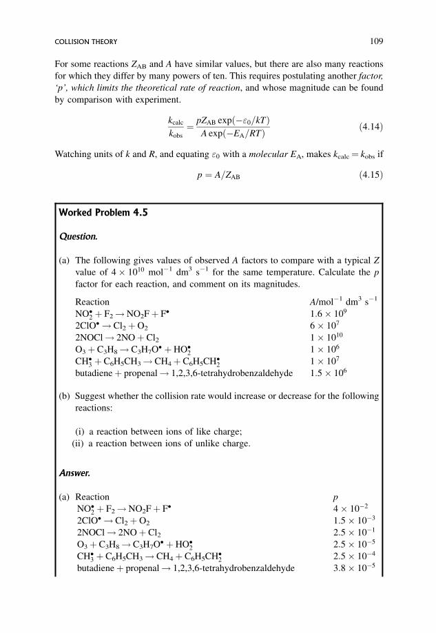
For some reactions ZAB and A have similar values, but there are also many reactions
for which they differ by many powers of ten. This requires postulating another factor,
‘p’, which limits the theoretical rate of reaction, and whose magnitude can be found
by comparison with experiment.
kcalc
kobs
¼ pZAB exp �"0=kTð ÞA exp �EA=RTð Þ ð4:14Þ
Watching units of k and R, and equating "0 with a molecular EA, makes kcalc¼ kobs if
p ¼ A=ZAB ð4:15Þ
Worked Problem 4.5
Question.
(a) The following gives values of observed A factors to compare with a typical Z
value of 4 1010 mol�1 dm3 s�1 for the same temperature. Calculate the p
factor for each reaction, and comment on its magnitudes.
Reaction A/mol�1 dm3 s�1
NO�2 þ F2!NO2Fþ F� 1:6 109
2ClO� ! Cl2þO2 6 107
2NOCl! 2NOþ Cl2 1 1010
O3þ C3H8! C3H7O� þHO�2 1 106
CH�3 þ C6H5CH3! CH4þ C6H5CH�2 1 107
butadieneþ propenal! 1,2,3,6-tetrahydrobenzaldehyde 1:5 106
(b) Suggest whether the collision rate would increase or decrease for the following
reactions:
(i) a reaction between ions of like charge;
(ii) a reaction between ions of unlike charge.
Answer.
(a) Reaction p
NO�2 þ F2!NO2Fþ F� 4 10�2
2ClO� ! Cl2þO2 1:5 10�3
2NOCl! 2NOþ Cl2 2:5 10�1
O3þ C3H8! C3H7O� þHO�2 2:5 10�5
CH�3 þ C6H5CH3! CH4þ C6H5CH�2 2:5 10�4
butadieneþ propenal! 1,2,3,6-tetrahydrobenzaldehyde 3:8 10�5
COLLISION THEORY 109
As the complexity of the reactants increases the p factor decreases, and the
discrepancy with collision theory increases. This reflects the inadequacy of simple
collision theory, especially the neglect of the internal structures of the reactants,
and intermolecular interactions.
(b) The latter effect becomes particularly important when considering reactions
between charged species:
(i) there will be strong attractive forces between the reactants and this would
be expected to increase the collision rate;
(ii) there will be strong repulsive forces leading to a decrease in collision rate.
This ‘p’ factor has also been interpreted as a preference for a certain direction, or
angle of approach, of the reacting molecules. Molecular beam experiments show
some reactions to have a quite decided preference for a specific direction and/or angle
of approach.
The ‘p’ factor could also be a consequence of the physically naıve hard sphere
model used. This model requires that there be no intermolecular interactions either at
close distances or at a distance. This has been shown not to be the case, with evidence
coming from many aspects of physical chemistry. Also, vibrations and rotations do
affect reaction, as is shown by experiments with molecular beams.
4.1.4 Reaction between like molecules
The rate of reaction can be calculated in a similar way, making sure that each A
molecule is not counted twice – each A molecule can be considered as both ‘hitting’
and being ‘hit by’ another A molecule.
k ¼ ZAAð�"0=kTÞ ð4:16Þwhere
ZAA ¼ ð32�kT=�Þ1=2r2
A ð4:17Þ
4.2 Modified Collision Theory
4.2.1 A new definition of a collision
Here a collision is seen in terms of the deflection of the molecules from their original
paths as they approach each other. Molecular beam experiments are ideally suited to
110 THEORIES OF CHEMICAL REACTIONS
study collisions. Two beams of molecules are shot at 90� to each other. Several things
can happen at the point of intersection of the beams.
� Both A and B molecules can continue on undeflected along the original direction of
the beam. They are unscattered.
� A and B molecules can interact and as a result be deflected from their original
trajectories. They are scattered.
The beam experiments detect scattered and unscattered A and B molecules. Any A
or B deflected and scattered must have collided.
In simple collision theory, if the impact parameter b � rA þ rB, then collision will
occur; if b > rA þ rB collision cannot occur. In molecular beam studies a collision is
still defined in terms of a distance apart of the trajectories, but this is no longer
rAþ rB, but is a distance bmax. If the impact parameter b � bmax, collision occurs, and
the numerical value of bmax is found from scattering experiments and is closely
related to the minimum angle of scattering able to be detected.
The impact parameter is defined as before (Figure 4.2 and Section 4.1.1).
Within the range of impact parameters from b¼ 0 to b¼1 there is a critical range
of values which result in collision.
� If b¼ 0 there will be a head-on collision
� If b < bmax there will be a collision
� If b > bmax there can be no collision
� If b¼ bmax the encounter has just been successful as a collision.
With this definition of a collision the cross sectional area is now
� ¼ �b2max ð4:18Þ
and this cross section is closely related to the rate constant. Each impact parameter is
associated with a particular value of the angle of scattering: b¼ 0 corresponds to a
‘head-on’ collision which results in totally backward scattering at 180�, whereas if b
is just less than bmax interactions will be small, resulting in a very small angle of
scattering. Intermediate situations, resulting in stronger interactions, lead to scattering
between 0 and 180�. If b > bmax there will be no collision and no scattering
(Figure 4.3).
The crucial parameter is thus bmax, and its magnitude can be found from
experiment.
4.2.2 Reactive collisions
When reaction occurs then successful collisions are detected from the scattering
patterns of products. These give an effective bmax1, and cross section for reaction,
MODIFIED COLLISION THEORY 111
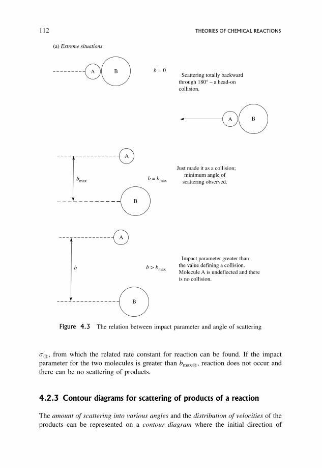
�1, from which the related rate constant for reaction can be found. If the impact
parameter for the two molecules is greater than bmax1, reaction does not occur and
there can be no scattering of products.
4.2.3 Contour diagrams for scattering of products of a reaction
The amount of scattering into various angles and the distribution of velocities of the
products can be represented on a contour diagram where the initial direction of
A B
A
B
A B
B
A
bmax b = bmax
b > bmax
b = 0
(a) Extreme situations
Scattering totally backwardthrough 180° _ a head-oncollision.
Just made it as a collision;minimum angle of
scattering observed.
Impact parameter greater thanthe value defining a collision. Molecule A is undeflected and there is no collision.
b
Figure 4.3 The relation between impact parameter and angle of scattering
112 THEORIES OF CHEMICAL REACTIONS
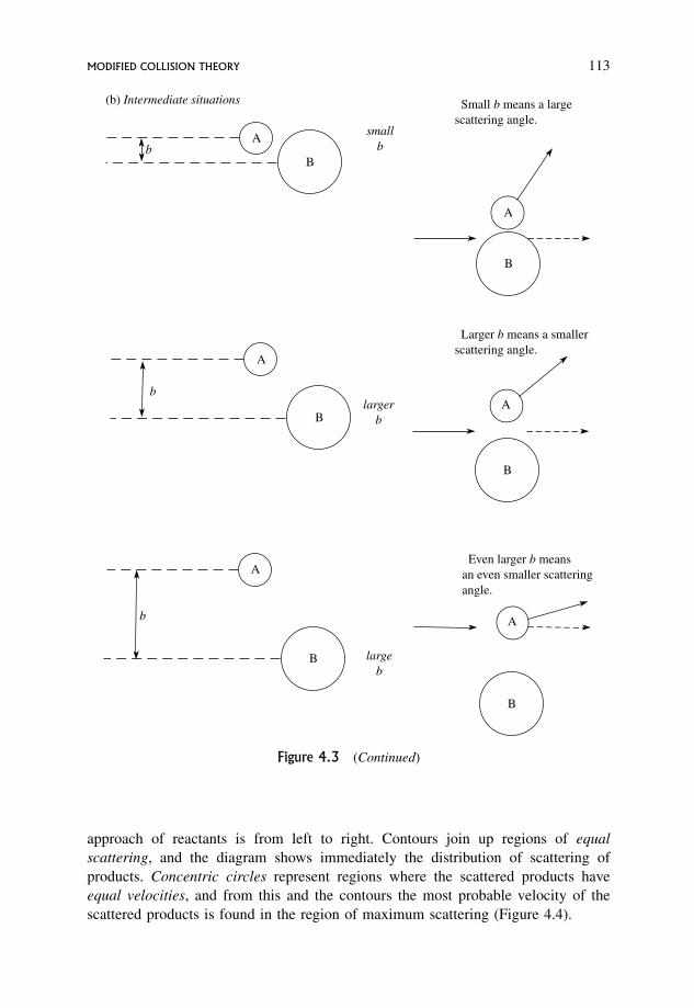
approach of reactants is from left to right. Contours join up regions of equal
scattering, and the diagram shows immediately the distribution of scattering of
products. Concentric circles represent regions where the scattered products have
equal velocities, and from this and the contours the most probable velocity of the
scattered products is found in the region of maximum scattering (Figure 4.4).
B
A
b
b
smallb
largerb
largeb
(b) Intermediate situations
B
A
b
B
A
B
A
Small b means a large scattering angle.
Larger b means a smallerscattering angle.
Even larger b meansan even smaller scatteringangle.
B
A
B
A
Figure 4.3 (Continued)
MODIFIED COLLISION THEORY 113
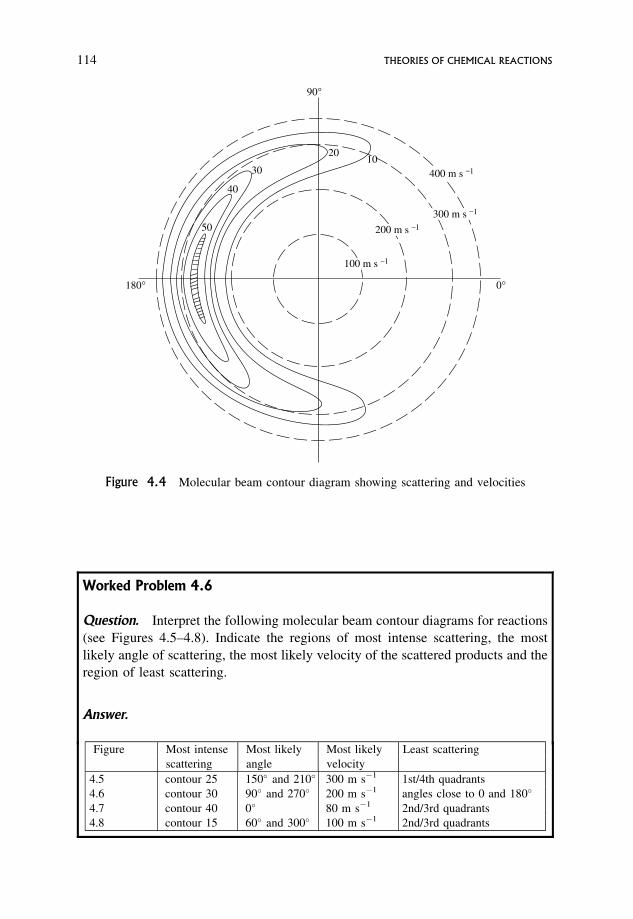
Worked Problem 4.6
Question. Interpret the following molecular beam contour diagrams for reactions
(see Figures 4.5–4.8). Indicate the regions of most intense scattering, the most
likely angle of scattering, the most likely velocity of the scattered products and the
region of least scattering.
Answer.
90°
180°
1020
30
40
50
0°
100 m s _1
300 m s _1
400 m s _1
200 m s _1
Figure 4.4 Molecular beam contour diagram showing scattering and velocities
Figure Most intense
scattering
Most likely
angle
Most likely
velocity
Least scattering
4.5 contour 25 150� and 210� 300 m s�1 1st/4th quadrants
4.6 contour 30 90� and 270� 200 m s�1 angles close to 0 and 180�
4.7 contour 40 0� 80 m s�1 2nd/3rd quadrants
4.8 contour 15 60� and 300� 100 m s�1 2nd/3rd quadrants
114 THEORIES OF CHEMICAL REACTIONS
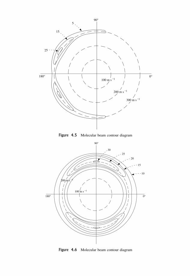
0°180°
90°
100 m s _1
200 m s _1
5
15
25
300 m s _1
Figure 4.5 Molecular beam contour diagram
15
20
25
30
90°
180°
200 m s _1
100 m s _1
0°
10
Figure 4.6 Molecular beam contour diagram
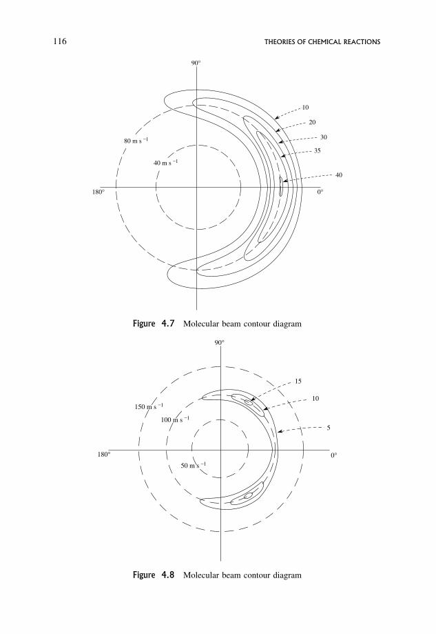
10
90°
180° 0°
20
30
35
40
80 m s _1
40 m s _1
Figure 4.7 Molecular beam contour diagram
15
10
5
0°180°
90°
150 m s _1
100 m s _1
50 m s _1
Figure 4.8 Molecular beam contour diagram
116 THEORIES OF CHEMICAL REACTIONS
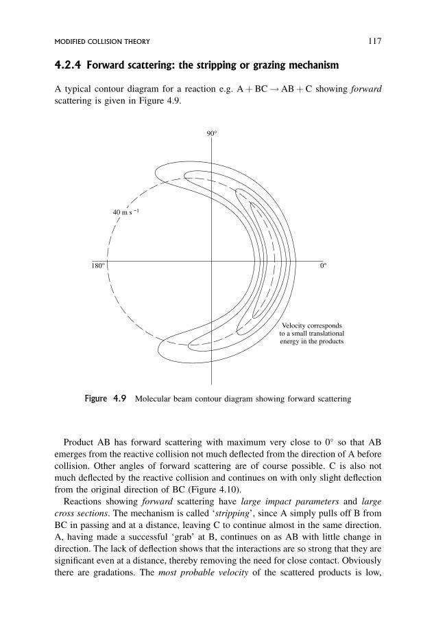
4.2.4 Forward scattering: the stripping or grazing mechanism
A typical contour diagram for a reaction e.g. Aþ BC!ABþ C showing forward
scattering is given in Figure 4.9.
Product AB has forward scattering with maximum very close to 0� so that AB
emerges from the reactive collision not much deflected from the direction of A before
collision. Other angles of forward scattering are of course possible. C is also not
much deflected by the reactive collision and continues on with only slight deflection
from the original direction of BC (Figure 4.10).
Reactions showing forward scattering have large impact parameters and large
cross sections. The mechanism is called ‘stripping’, since A simply pulls off B from
BC in passing and at a distance, leaving C to continue almost in the same direction.
A, having made a successful ‘grab’ at B, continues on as AB with little change in
direction. The lack of deflection shows that the interactions are so strong that they are
significant even at a distance, thereby removing the need for close contact. Obviously
there are gradations. The most probable velocity of the scattered products is low,
90°
180° 0°
Velocity correspondsto a small translationalenergy in the products
40 m s _1
Figure 4.9 Molecular beam contour diagram showing forward scattering
MODIFIED COLLISION THEORY 117
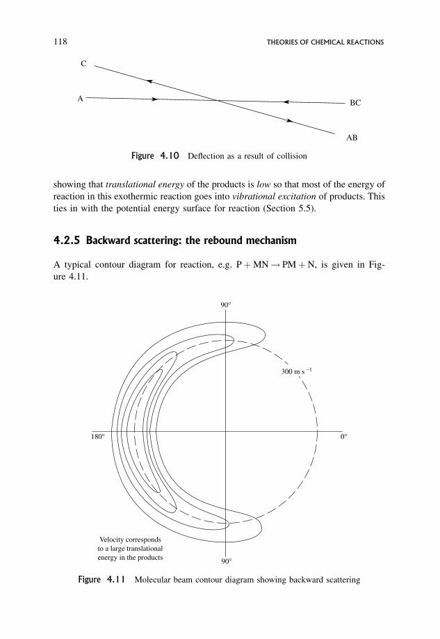
showing that translational energy of the products is low so that most of the energy of
reaction in this exothermic reaction goes into vibrational excitation of products. This
ties in with the potential energy surface for reaction (Section 5.5).
4.2.5 Backward scattering: the rebound mechanism
A typical contour diagram for reaction, e.g. PþMN! PMþN, is given in Fig-
ure 4.11.
C
A BC
AB
Figure 4.10 Deflection as a result of collision
90°
90°
180° 0°
Velocity correspondsto a large translationalenergy in the products
300 m s _1
Figure 4.11 Molecular beam contour diagram showing backward scattering
118 THEORIES OF CHEMICAL REACTIONS
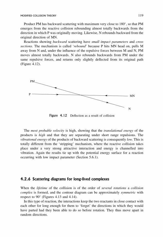
Product PM has backward scattering with maximum very close to 180�, so that PM
emerges from the reactive collision rebounding almost totally backwards from the
direction in which P was originally moving. Likewise, N rebounds backward from the
original direction of MN.
Reactions showing backward scattering have small impact parameters and cross
sections. The mechanism is called ‘rebound’ because P hits MN head on, pulls M
away from N and, under the influence of the repulsive forces between M and N, PM
moves almost totally backwards. N also rebounds backwards from PM under the
same repulsive forces, and returns only slightly deflected from its original path
(Figure 4.12).
The most probable velocity is high, showing that the translational energy of the
products is high and that they are separating under short range repulsions. The
vibrational energy of the products of backward scattering is consequently low. This is
totally different from the ‘stripping’ mechanism, where the reactive collision takes
place under a very strong attractive interaction and energy is channelled into
vibration. Again the results tie up with the potential energy surface for a reaction
occurring with low impact parameter (Section 5.6.1).
4.2.6 Scattering diagrams for long-lived complexes
When the lifetime of the collision is of the order of several rotations a collision
complex is formed, and the contour diagram can be approximately symmetric with
respect to 90� (Figures 4.13 and 4.14).
In this type of reaction, the interactions keep the two reactants in close contact with
each other for long enough for them to ‘forget’ the directions in which they would
have parted had they been able to do so before rotation. They thus move apart in
random directions.
PM
P MN
N
Figure 4.12 Deflection as a result of collision
MODIFIED COLLISION THEORY 119
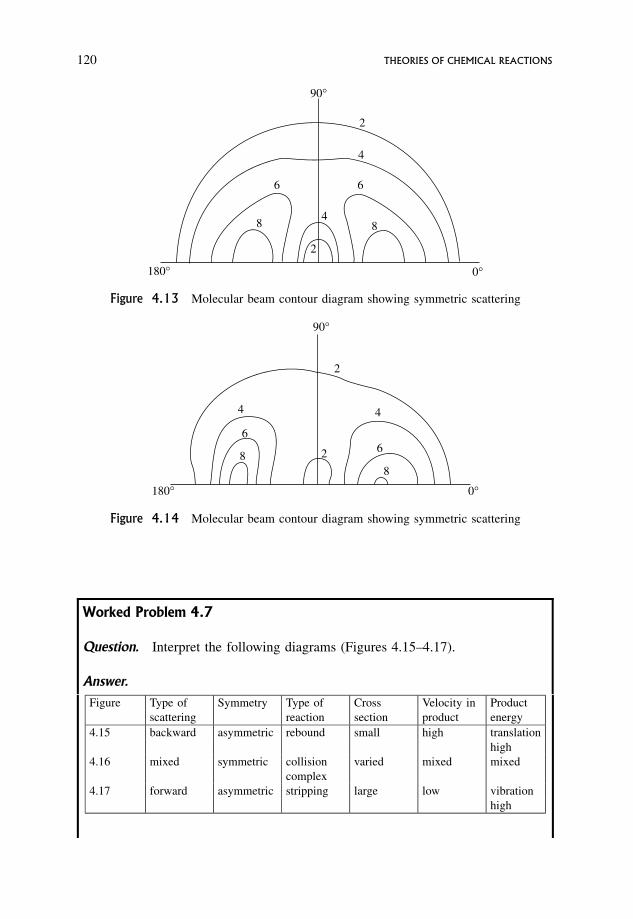
Worked Problem 4.7
Question. Interpret the following diagrams (Figures 4.15–4.17).
Answer.
180°
90°
0°
2
2
4
66
884
Figure 4.13 Molecular beam contour diagram showing symmetric scattering
180° 0°
90°
2
4
6
8 2 6
8
4
Figure 4.14 Molecular beam contour diagram showing symmetric scattering
Figure Type of
scattering
Symmetry Type of
reaction
Cross
section
Velocity in
product
Product
energy
4.15 backward asymmetric rebound small high translation
high
4.16 mixed symmetric collision
complex
varied mixed mixed
4.17 forward asymmetric stripping large low vibration
high
120 THEORIES OF CHEMICAL REACTIONS
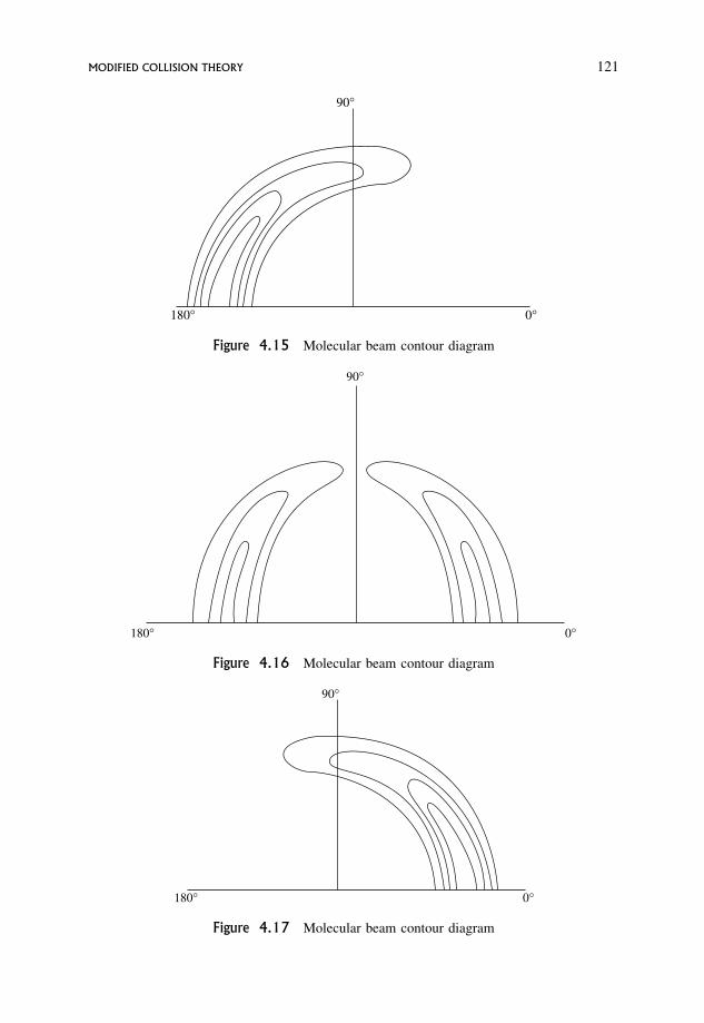
90°
180° 0°
Figure 4.15 Molecular beam contour diagram
180° 0°
90°
Figure 4.16 Molecular beam contour diagram
90°
180° 0°
Figure 4.17 Molecular beam contour diagram
MODIFIED COLLISION THEORY 121
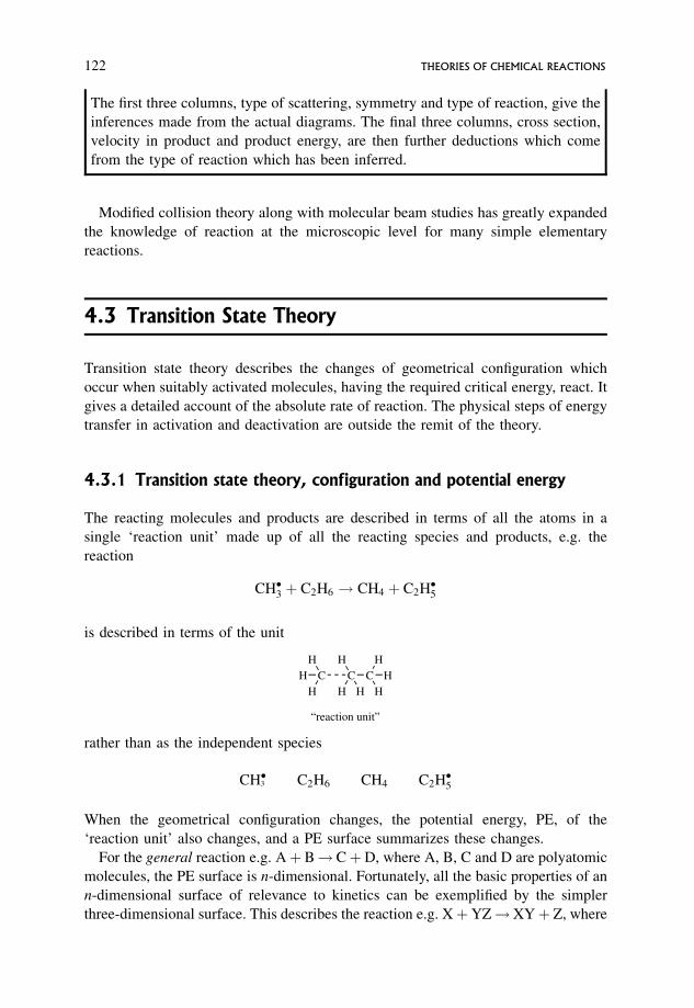
The first three columns, type of scattering, symmetry and type of reaction, give the
inferences made from the actual diagrams. The final three columns, cross section,
velocity in product and product energy, are then further deductions which come
from the type of reaction which has been inferred.
Modified collision theory along with molecular beam studies has greatly expanded
the knowledge of reaction at the microscopic level for many simple elementary
reactions.
4.3 Transition State Theory
Transition state theory describes the changes of geometrical configuration which
occur when suitably activated molecules, having the required critical energy, react. It
gives a detailed account of the absolute rate of reaction. The physical steps of energy
transfer in activation and deactivation are outside the remit of the theory.
4.3.1 Transition state theory, configuration and potential energy
The reacting molecules and products are described in terms of all the atoms in a
single ‘reaction unit’ made up of all the reacting species and products, e.g. the
reaction
CH�3 þ C2H6 ! CH4 þ C2H�5
is described in terms of the unit
H CH
HC
H
H HC
H
HH
“reaction unit”
rather than as the independent species
CH�3 C2H6 CH4 C2H�5
When the geometrical configuration changes, the potential energy, PE, of the
‘reaction unit’ also changes, and a PE surface summarizes these changes.
For the general reaction e.g. Aþ B! CþD, where A, B, C and D are polyatomic
molecules, the PE surface is n-dimensional. Fortunately, all the basic properties of an
n-dimensional surface of relevance to kinetics can be exemplified by the simpler
three-dimensional surface. This describes the reaction e.g. XþYZ!XYþ Z, where
122 THEORIES OF CHEMICAL REACTIONS
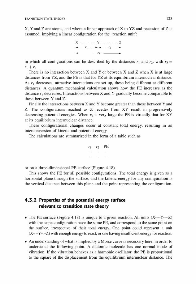
X, Y and Z are atoms, and where a linear approach of X to YZ and recession of Z is
assumed, implying a linear configuration for the ‘reaction unit’:
X Y Zr1 r2
r3
in which all configurations can be described by the distances r1 and r2, with r3¼r1þ r2.
There is no interaction between X and Y or between X and Z when X is at large
distances from YZ, and the PE is that for YZ at its equilibrium internuclear distance.
As r1 decreases, attractive interactions are set up, these being different at different
distances. A quantum mechanical calculation shows how the PE increases as the
distance r1 decreases. Interactions between X and Y gradually become comparable to
these between Y and Z.
Finally the interactions between X and Y become greater than those between Y and
Z. The configurations reached as Z recedes from XY result in progressively
decreasing potential energies. When r2 is very large the PE is virtually that for XY
at its equilibrium internuclear distance.
These configurational changes occur at constant total energy, resulting in an
interconversion of kinetic and potential energy.
The calculations are summarized in the form of a table such as
r1 r2 PE
-- -- --
-- -- --
or on a three-dimensional PE surface (Figure 4.18).
This shows the PE for all possible configurations. The total energy is given as a
horizontal plane through the surface, and the kinetic energy for any configuration is
the vertical distance between this plane and the point representing the configuration.
4.3.2 Properties of the potential energy surface
relevant to transition state theory
� The PE surface (Figure 4.18) is unique to a given reaction. All units (X----Y----Z)
with the same configuration have the same PE, and correspond to the same point on
the surface, irrespective of their total energy. One point could represent a unit
(X----Y----Z) with enough energy to react, or one having insufficient energy for reaction.
� An understanding of what is implied by a Morse curve is necessary here, in order to
understand the following point. A diatomic molecule has one normal mode of
vibration. If the vibration behaves as a harmonic oscillator, the PE is proportional
to the square of the displacement from the equilibrium internuclear distance. The
TRANSITION STATE THEORY 123
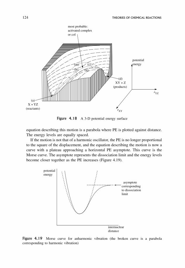
equation describing this motion is a parabola where PE is plotted against distance.
The energy levels are equally spaced.
If the motion is not that of a harmonic oscillator, the PE is no longer proportional
to the square of the displacement, and the equation describing the motion is now a
curve with a plateau approaching a horizontal PE asymptote. This curve is the
Morse curve. The asymptote represents the dissociation limit and the energy levels
become closer together as the PE increases (Figure 4.19).
(d)XY + Z
(products)
potentialenergy
rYZ
rXY
(a)X + YZ
(reactants)
most probable:activated complexor col
(m)
(b) (n)
(c)
Figure 4.18 A 3-D potential energy surface
potentialenergy
internucleardistance
asymptote correspondingto dissociationlimit
Figure 4.19 Morse curve for anharmonic vibration (the broken curve is a parabola
corresponding to harmonic vibration)
124 THEORIES OF CHEMICAL REACTIONS
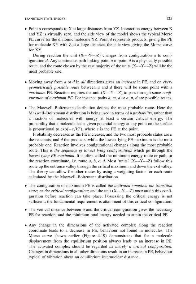
� Point a corresponds to X at large distances from YZ. Interaction energy between X
and YZ is virtually zero, and the side view of the model shows the typical Morse
PE curve for the diatomic molecule YZ. Point d represents products, giving the PE
for molecule XY with Z at a large distance, the side view giving the Morse curve
for XY.
During reaction the unit (X----Y----Z) changes from configuration a to conf-
iguration d. Any continuous path linking point a to point d is a physically possible
route, and the route chosen by the vast majority of the units (X----Y----Z) will be the
most probable one.
� Moving away from a or d in all directions gives an increase in PE, and on every
geometrically possible route between a and d there will be some point with a
maximum PE. Reaction requires the unit (X----Y----Z) to pass through some confi-
guration of maximum PE. For instance paths a, m, d or a, n, d are possible routes.
� The Maxwell–Boltzmann distribution defines the most probable route. Here the
Maxwell–Boltzmann distribution is being used in terms of a probability, rather than
a fraction of molecules with energy at least a certain critical energy. The
probability that a molecule has a given potential energy at any point on the surface
is proportional to exp �"=kTð Þ, where " is the PE at the point.
Probability decreases as the PE increases, and the two most probable states are a
the reactants, and d the products, while the lowest lying PE maximum is the most
probable one. Reaction involves configurational changes along the most probable
route. This is the sequence of lowest lying configurations which go through the
lowest lying PE maximum. It is often called the minimum energy route or path, or
the reaction coordinate, i.e. route a, b, c, d. Most ‘units’ (X----Y----Z) follow this
route up the entrance valley through the critical maximum and down the exit valley.
The theory can allow for other routes by using a weighting factor for each route
calculated by the Maxwell–Boltzmann distribution.
� The configuration of maximum PE is called the activated complex; the transition
state; or the critical configuration; and the unit (X----Y----Z) must attain this confi-
guration before reaction can take place. Possessing the critical energy is not
sufficient; the fundamental requirement is attainment of this critical configuration.
� The vertical distance between a and the critical configuration gives the necessary
PE for reaction, and the minimum total energy needed to attain the critical PE.
� Any change in the dimensions of the activated complex along the reaction
coordinate leads to a decrease in PE, behaviour not found in molecules. The
Morse curve shown earlier (Figure 4.19) demonstrates that for a molecule
displacement from the equilibrium position always leads to an increase in PE.
The activated complex should be regarded as merely a critical configuration.
Changes in dimensions in all other directions result in an increase in PE, behaviour
typical of vibration about an equilibrium internuclear distance.
TRANSITION STATE THEORY 125
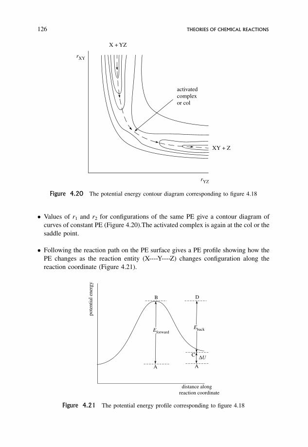
� Values of r1 and r2 for configurations of the same PE give a contour diagram of
curves of constant PE (Figure 4.20).The activated complex is again at the col or the
saddle point.
� Following the reaction path on the PE surface gives a PE profile showing how the
PE changes as the reaction entity (X----Y----Z) changes configuration along the
reaction coordinate (Figure 4.21).
activated complexor col
XY + Z
X + YZ
rXY
rYZ
Figure 4.20 The potential energy contour diagram corresponding to figure 4.18
EforwardEback
A
DB
A
distance alongreaction coordinate
pote
ntia
l ene
rgy
C ∆U
Figure 4.21 The potential energy profile corresponding to figure 4.18
126 THEORIES OF CHEMICAL REACTIONS
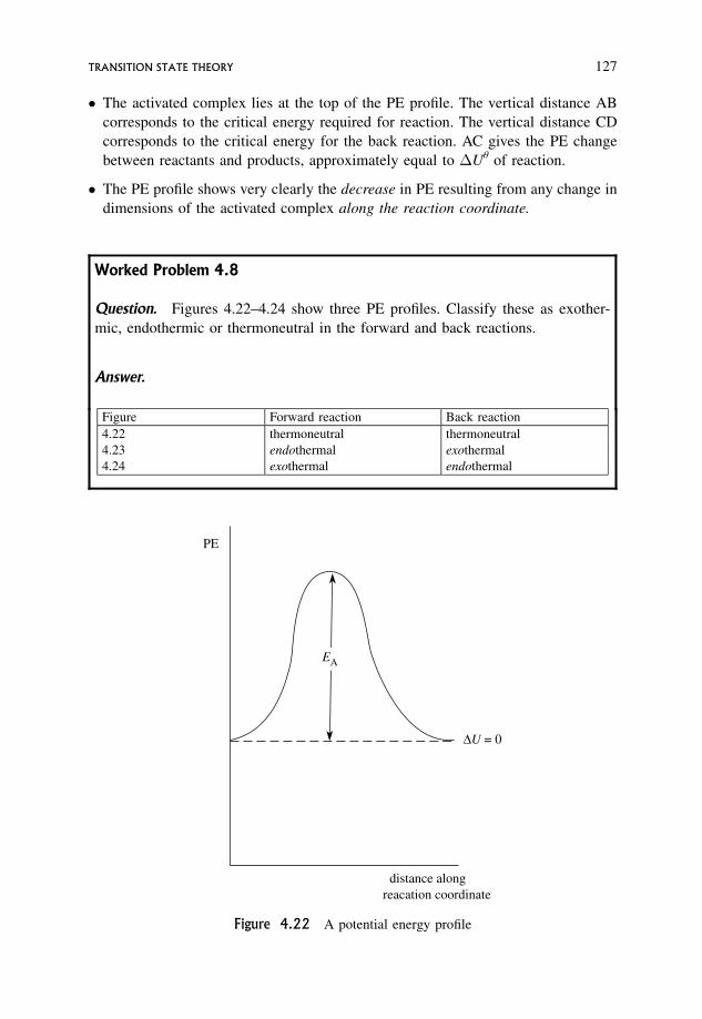
� The activated complex lies at the top of the PE profile. The vertical distance AB
corresponds to the critical energy required for reaction. The vertical distance CD
corresponds to the critical energy for the back reaction. AC gives the PE change
between reactants and products, approximately equal to �U of reaction.
� The PE profile shows very clearly the decrease in PE resulting from any change in
dimensions of the activated complex along the reaction coordinate.
Worked Problem 4.8
Question. Figures 4.22–4.24 show three PE profiles. Classify these as exother-
mic, endothermic or thermoneutral in the forward and back reactions.
Answer.
EA
distance alongreacation coordinate
∆U = 0
PE
Figure 4.22 A potential energy profile
Figure Forward reaction Back reaction
4.22 thermoneutral thermoneutral
4.23 endothermal exothermal
4.24 exothermal endothermal
TRANSITION STATE THEORY 127
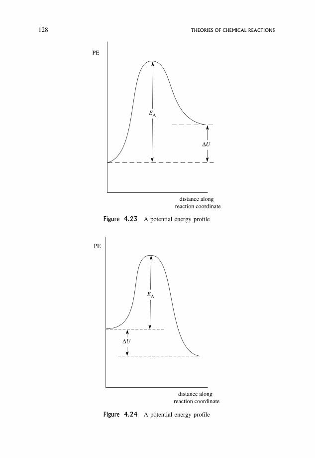
EA
∆U
PE
distance alongreaction coordinate
Figure 4.23 A potential energy profile
EA
distance alongreaction coordinate
PE
∆U
Figure 4.24 A potential energy profile
128 THEORIES OF CHEMICAL REACTIONS
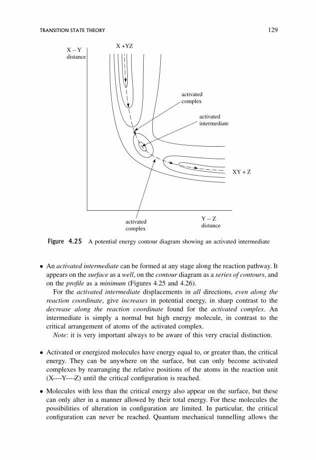
� An activated intermediate can be formed at any stage along the reaction pathway. It
appears on the surface as a well, on the contour diagram as a series of contours, and
on the profile as a minimum (Figures 4.25 and 4.26).
For the activated intermediate displacements in all directions, even along the
reaction coordinate, give increases in potential energy, in sharp contrast to the
decrease along the reaction coordinate found for the activated complex. An
intermediate is simply a normal but high energy molecule, in contrast to the
critical arrangement of atoms of the activated complex.
Note: it is very important always to be aware of this very crucial distinction.
� Activated or energized molecules have energy equal to, or greater than, the critical
energy. They can be anywhere on the surface, but can only become activated
complexes by rearranging the relative positions of the atoms in the reaction unit
(X----Y----Z) until the critical configuration is reached.
� Molecules with less than the critical energy also appear on the surface, but these
can only alter in a manner allowed by their total energy. For these molecules the
possibilities of alteration in configuration are limited. In particular, the critical
configuration can never be reached. Quantum mechanical tunnelling allows the
activatedcomplex
activatedintermediate
activatedcomplex
Y -- Zdistance
X -- Ydistance
XY + Z
X +YZ
Figure 4.25 A potential energy contour diagram showing an activated intermediate
TRANSITION STATE THEORY 129

possibility that products can be reached without the reactants having the critical
energy. Tunnelling appears as a possibility when the reaction process is treated
quantum mechanically. Reaction treated classically requires the unit (X----Y---- Z)
to pass over the top of the col, i.e. through the critical configuration. But, if
movement over the surface is quantized, there is a finite probability that the unit
(X- - -Y- - -Z) can move from a point on the reactant side of the barrier to another
point on the product side without passing over the barrier. This is tunnelling, and
reaction has occurred without the reactants having the critical energy. The result is
that the transmission coefficient (Section 4.3.3) is greater than unity. Tunnelling is
more likely for reactions of light mass species, such as H, Hþ, H� or electrons.
This is a refinement on basic transition state theory not dealt with here.
� The process of reaction is often described as ‘moving over the PE surface’. This is
not a movement in space, but only an internal movement of atoms with respect to
each other. Likewise, phrases such as ‘surmounting a PE barrier’ or ‘getting over
the energy hump’ and ‘climbing up and over the col or saddle point’ are descriptive
only, and the term ‘the rate of passage through the critical configuration’ simply
means a rate of change of configuration.
� The critical configuration occupies a flat non-zero area, corresponding to a flat non-
zero length along the reaction coordinate. The potential energy is virtually constant
over that part of the surface defining the activated complex, with zero force acting
on the critical configuration. This results in a constant rate of change in
configuration through the critical configuration. This describes a free translation
along the reaction coordinate. Once the system reaches configurations with
decreasing PE, the motion ceases to be a free translation.
pote
ntia
l ene
rgy
distance alongreaction coordinate
Figure 4.26 A potential energy profile showing an activated intermediate
130 THEORIES OF CHEMICAL REACTIONS
� It is vitally important to understand what a free translation means, and to be aware
of the important consequences of motion through the critical configuration being a
free translation. The force acting on a system is
force ¼ � dðPEÞdr
ð4:19Þ
If the PE is constant, then dðPEÞ=dr is zero, and the force is zero and there is no
acceleration in the motion of the reaction unit as it passes through the critical
configuration, i.e. through the region of the surface where the PE is constant. If
there is no acceleration, then the reaction unit must pass over the barrier at a
constant rate. This rate can be calculated from kinetic theory.
If the PE is not constant, then dðPEÞ=dr is non-zero, and the rate of change of
configuration over that region of the PE surface will vary depending on the value of
dðPEÞ=dr. This happens at all points other than the critical configuration.
� The concentration of activated complexes is the total number of units (X----Y----Z)
per unit volume which are in the critical configuration, no matter what their past
history is.
� The rate of reaction is the total number of units (X----Y----Z) per unit volume which
pass through the critical configuration per unit time from reactant valley to product
valley.
Worked Problem 4.9
Question. Figure 4.27 gives a potential energy contour diagram. What can be said
about configurations along the line AB? Identify the activated complex and
activated intermediate in the diagram.
Answer. Along AB, rAB¼ rBC. The activated complex lies at the saddle-point
lying on AB. The PE contour diagram is symmetrical about the critical configura-
tion. The activated intermediate lies in the well of the elliptical contours and at
configurations where rBC > rAB. There is a further activated complex as marked
along the line PQ.
4.3.3 An outline of arguments involved in the
derivation of the rate equation
This involves calculating the rate at which the ‘reaction unit’ passes through the
critical configuration. Since the PE is constant over the region of the surface occupied
by the critical configuration, the rate at which it moves through the critical
TRANSITION STATE THEORY 131
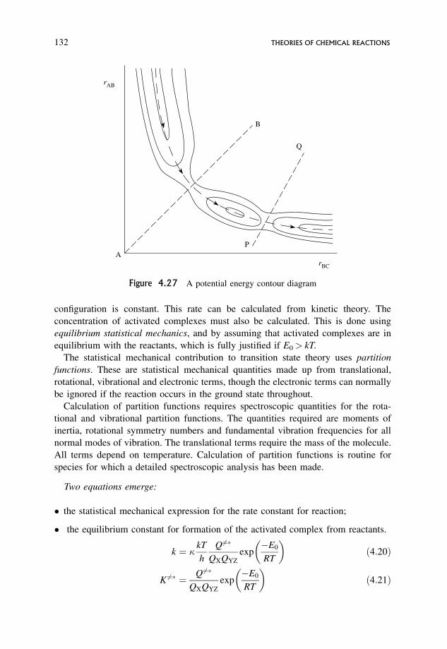
configuration is constant. This rate can be calculated from kinetic theory. The
concentration of activated complexes must also be calculated. This is done using
equilibrium statistical mechanics, and by assuming that activated complexes are in
equilibrium with the reactants, which is fully justified if E0 > kT.
The statistical mechanical contribution to transition state theory uses partition
functions. These are statistical mechanical quantities made up from translational,
rotational, vibrational and electronic terms, though the electronic terms can normally
be ignored if the reaction occurs in the ground state throughout.
Calculation of partition functions requires spectroscopic quantities for the rota-
tional and vibrational partition functions. The quantities required are moments of
inertia, rotational symmetry numbers and fundamental vibration frequencies for all
normal modes of vibration. The translational terms require the mass of the molecule.
All terms depend on temperature. Calculation of partition functions is routine for
species for which a detailed spectroscopic analysis has been made.
Two equations emerge:
� the statistical mechanical expression for the rate constant for reaction;
� the equilibrium constant for formation of the activated complex from reactants.
k ¼ �kT
h
Q6¼�
QXQYZ
exp�E0
RT
� �ð4:20Þ
K 6¼� ¼ Q6¼�
QXQYZ
exp�E0
RT
� �ð4:21Þ
B
Q
PA
rAB
rBC
Figure 4.27 A potential energy contour diagram
132 THEORIES OF CHEMICAL REACTIONS
� is the transmission coefficient and allows for the possibility that not all units (X----
Y----Z) in the critical configuration may actually react, k and h are the Boltzmann and
Planck constants, E0 is the critical energy and can be found from the PE surface, Q6¼�
is the partition function per unit volume for the activated complex with one term
missing and QX and QYZ are ordinary complete partition functions per unit volume
for the reactants. Like Q6¼�, K 6¼� is a quantity with one term missing. This is explained
in the brief derivation given below.
Equation (4.20) is the working equation of transition state theory in statistical
mechanical form.
Brief derivation of transition state theory
Reaction occurs when the reaction unit attains the critical configuration, becomes an
activated complex, and passes on to product. The critical configuration occurs at the
maximum on the potential energy profile and extends over a length � along
the reaction coordinate. The activated complex spends a time in the critical
configuration, and from this the rate of passage through the critical configuration
from left to right is given as
v ¼ �
where the magnitudes of both � and are unspecified.
If N 6¼ is the total number of activated complexes, then the number which pass
through the critical configuration per unit time per unit volume is N 6¼v=V�, and so the
rate of reaction can be given as
�N 6¼v
V�¼ �c 6¼v
�ð4:22Þ
where � is the transmission coefficient which accounts for the possibility that not all
activated complexes reach product configuration, and c6¼ is the concentration of
activated complexes expressed as a number of activated complexes per unit volume.
v can be found from kinetic theory, and is v ¼ kT=2��6¼� �1=2
, giving
rate of reaction ¼ �c 6¼
�
kT
2��6¼
� �1=2
ð4:23Þ
where � 6¼ is the reduced mass for the change of configuration, calculable from the
potential energy surface, but generally left unspecified.
The rate of reaction can also be given as kcXcYZ so that the calculated rate constant
is given by
k ¼ �c6¼
cXcYZ
1
�
kT
2��6¼
� �1=2
ð4:24Þ
TRANSITION STATE THEORY 133
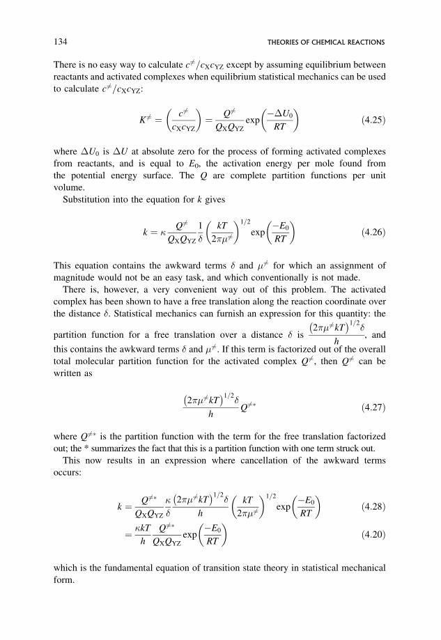
There is no easy way to calculate c6¼=cXcYZ except by assuming equilibrium between
reactants and activated complexes when equilibrium statistical mechanics can be used
to calculate c 6¼=cXcYZ:
K 6¼ ¼ c6¼
cXcYZ
� �¼ Q 6¼
QXQYZ
exp��U0
RT
� �ð4:25Þ
where �U0 is �U at absolute zero for the process of forming activated complexes
from reactants, and is equal to E0, the activation energy per mole found from
the potential energy surface. The Q are complete partition functions per unit
volume.
Substitution into the equation for k gives
k ¼ �Q 6¼
QXQYZ
1
�
kT
2��6¼
� �1=2
exp�E0
RT
� �ð4:26Þ
This equation contains the awkward terms � and �6¼ for which an assignment of
magnitude would not be an easy task, and which conventionally is not made.
There is, however, a very convenient way out of this problem. The activated
complex has been shown to have a free translation along the reaction coordinate over
the distance �. Statistical mechanics can furnish an expression for this quantity: the
partition function for a free translation over a distance � is2��6¼kT� �1=2
�
h, and
this contains the awkward terms � and � 6¼. If this term is factorized out of the overall
total molecular partition function for the activated complex Q 6¼, then Q 6¼ can be
written as
2��6¼kT� �1=2
�
hQ6¼� ð4:27Þ
where Q 6¼� is the partition function with the term for the free translation factorized
out; the * summarizes the fact that this is a partition function with one term struck out.
This now results in an expression where cancellation of the awkward terms
occurs:
k ¼ Q 6¼�
QXQYZ
�
�
2�� 6¼kT� �1=2
�
h
kT
2��6¼
� �1=2
exp�E0
RT
� �ð4:28Þ
¼ �kT
h
Q 6¼�
QXQYZ
exp�E0
RT
� �ð4:20Þ
which is the fundamental equation of transition state theory in statistical mechanical
form.
134 THEORIES OF CHEMICAL REACTIONS
Calculation of the partition functions for reactants is straightforward, but the
partition function for the activated complex needs explanation. The activated complex
has been shown to have the unique feature of a free translation along the reaction
coordinate over the distance occupied by the activated complex. The statistical
mechanical quantity for this free translation has already been factorized out from the
total partition function for the activated complex in the derivation. This has been done
simply because doing so allows cancellation of some awkward terms in the derivation
of the rate constant equation. This is why the symbol has * appeared along with the
symbol 6¼, this latter indicating that the process is one of forming the activated
complex, often very loosely termed activation. Q 6¼� is now a partition function
per unit volume for the activated complex but with one crucial term missing from
it, i.e. the term for the free translation. This is more fully explained in the section
below.
4.3.4 Use of the statistical mechanical form of transition state theory
E0 can be calculated from the PE surface, and if Q6¼�, QX and QYZ can be calculated
then a completely theoretical calculation would give k, the absolute rate constant for
the given reaction.
Calculation of partition functions for reactants is a routine matter if a complete
spectroscopic analysis is available.
The partition function calculation for the activated complex is more tricky. If the
surface is known the quantities quoted above can be found from the dimensions and
the curvature of the surface around the critical configuration. If this is not possible,
then estimates of Q 6¼� can be made by analogy with a molecule of similar structure.
The vital feature is that the free translation along the reaction coordinate has already
been accounted for and must not be included in the calculation, and so the activated
complex has one degree of vibrational freedom less than that for a molecule with the
same number of atoms.
The statistical mechanical form of transition theory makes considerable use of the
concepts of translational, rotational and vibrational degrees of freedom. For a system
made up of N atoms, 3N coordinates are required to completely specify the positions
of all the atoms. Three coordinates are required to specify translational motion in
space. For a linear molecule, two coordinates are required to specify rotation of the
molecule as a whole, while for a non-linear molecule three coordinates are required.
These correspond to two and three rotational modes respectively. This leaves 3N � 5
(linear) or 3N � 6 (non-linear) coordinates to specify vibrations in the molecule. If
the vibrations can be approximated to harmonic oscillators, these will correspond to
normal modes of vibration.
The number of coordinates needed to specify each type of motion is called the number
of degrees of freedom; e.g., non-linear molecules have three translational degrees
of freedom, three rotational degrees of freedom and 3N � 6 vibrational degrees of
freedom.
TRANSITION STATE THEORY 135
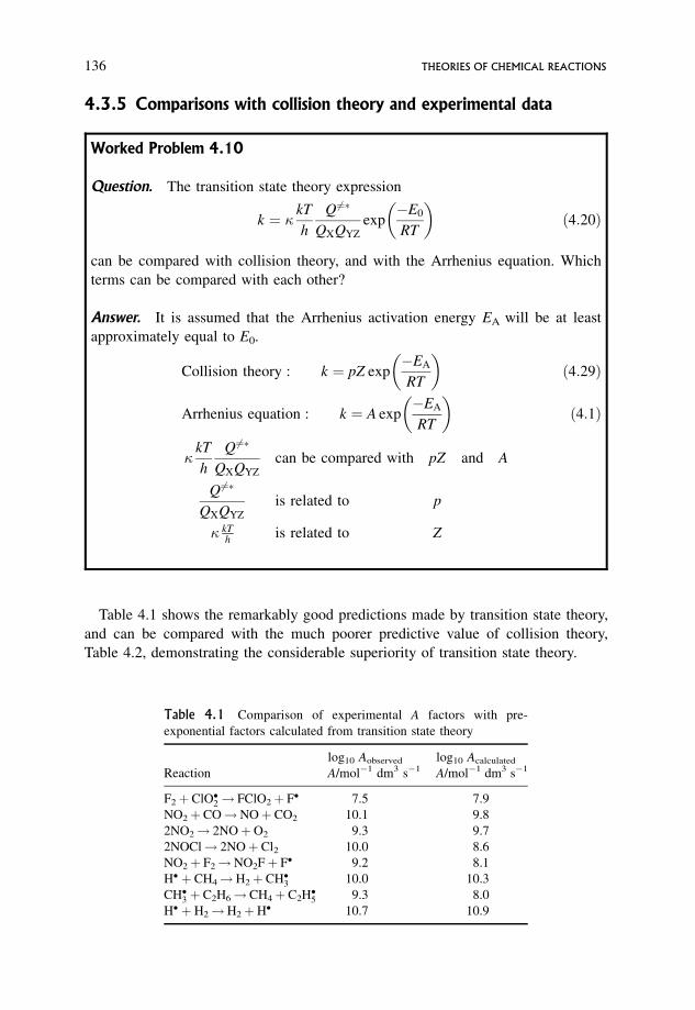
4.3.5 Comparisons with collision theory and experimental data
Worked Problem 4.10
Question. The transition state theory expression
k ¼ �kT
h
Q 6¼�
QXQYZ
exp�E0
RT
� �ð4:20Þ
can be compared with collision theory, and with the Arrhenius equation. Which
terms can be compared with each other?
Answer. It is assumed that the Arrhenius activation energy EA will be at least
approximately equal to E0.
Collision theory : k ¼ pZ exp�EA
RT
� �ð4:29Þ
Arrhenius equation : k ¼ A exp�EA
RT
� �ð4:1Þ
�kT
h
Q 6¼�
QXQYZ
can be compared with pZ and A
Q6¼�
QXQYZ
is related to p
� kTh
is related to Z
Table 4.1 shows the remarkably good predictions made by transition state theory,
and can be compared with the much poorer predictive value of collision theory,
Table 4.2, demonstrating the considerable superiority of transition state theory.
Table 4.1 Comparison of experimental A factors with pre-
exponential factors calculated from transition state theory
log10 Aobserved log10 Acalculated
Reaction A/mol�1 dm3 s�1 A/mol�1 dm3 s�1
F2þ ClO�2! FClO2þ F� 7.5 7.9
NO2þ CO!NOþ CO2 10.1 9.8
2NO2! 2NOþO2 9.3 9.7
2NOCl! 2NOþ Cl2 10.0 8.6
NO2þ F2!NO2Fþ F� 9.2 8.1
H� þ CH4!H2þ CH�3 10.0 10.3
CH�3 þ C2H6! CH4þ C2H�5 9.3 8.0
H� þH2!H2þH� 10.7 10.9
136 THEORIES OF CHEMICAL REACTIONS
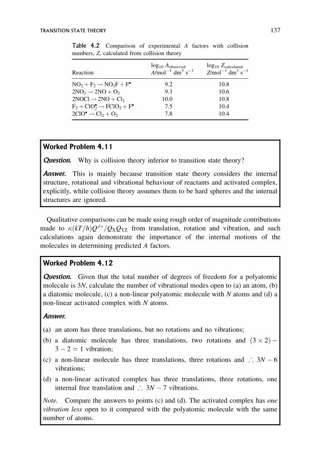
Worked Problem 4.11
Question. Why is collision theory inferior to transition state theory?
Answer. This is mainly because transition state theory considers the internal
structure, rotational and vibrational behaviour of reactants and activated complex,
explicitly, while collision theory assumes them to be hard spheres and the internal
structures are ignored.
Qualitative comparisons can be made using rough order of magnitude contributions
made to �ðkT=hÞQ6¼�=QXQYZ from translation, rotation and vibration, and such
calculations again demonstrate the importance of the internal motions of the
molecules in determining predicted A factors.
Worked Problem 4.12
Question. Given that the total number of degrees of freedom for a polyatomic
molecule is 3N, calculate the number of vibrational modes open to (a) an atom, (b)
a diatomic molecule, (c) a non-linear polyatomic molecule with N atoms and (d) a
non-linear activated complex with N atoms.
Answer.
(a) an atom has three translations, but no rotations and no vibrations;
(b) a diatomic molecule has three translations, two rotations and ð3 2Þ�3� 2 ¼ 1 vibration;
(c) a non-linear molecule has three translations, three rotations and ; 3N � 6
vibrations;
(d) a non-linear activated complex has three translations, three rotations, one
internal free translation and ; 3N � 7 vibrations.
Note. Compare the answers to points (c) and (d). The activated complex has one
vibration less open to it compared with the polyatomic molecule with the same
number of atoms.
Table 4.2 Comparison of experimental A factors with collision
numbers, Z, calculated from collision theory
log10 Aobserved log10 Zcalculated
Reaction A/mol�1 dm3 s�1 Z/mol�1 dm3 s�1
NO2þ F2!NO2Fþ F� 9.2 10.8
2NO2! 2NOþO2 9.3 10.6
2NOCl! 2NOþ Cl2 10.0 10.8
F2þ ClO�2! FClO2þ F� 7.5 10.4
2ClO� ! Cl2þO2 7.8 10.4
TRANSITION STATE THEORY 137
It is also possible to look at the changes in types of degrees of freedom, and
changes in internal motions on forming the activated complex. Considerable insight
into trends in A factors, and interpretations of these in terms of changes in internal
motions, can be made using rough order of magnitude calculations without having
recourse to detailed accurate values for the partition functions. The approximations
made are acceptable because contributions from the internal motions do not vary
much with mass, moment of inertia or vibrational frequency.
Typical values of these contributions:
� for each translation: 109 to 1010 dm�1
� for each rotation: 10 to 102
� for each vibration: 1 to 10
Worked Problem 4.13
Question. At 298 K, and assuming � ¼ 1 and �kT=h ¼ 6:2 1012 s�1, and using
typical values (in the middle of the ranges above) for the contributions from
translation, rotation and vibration,
for each translation: 5 109 dm�1
for each rotation: 50
for each vibration 5
calculate the predicted A factor for the following reaction types:
(a) atomþ atom! activated complex;
(b) atomþ linear molecule! non-linear activated complex;
(c) two non-linear molecules! non-linear activated complex.
Answer.
(a) Each atom has three translations; the activated complex has three translations,
two rotations, one internal free translation and ;ð3 2Þ � 6 vibrations i.e.
zero. The contribution from the internal translation has already been incorpo-
rated in the derivation, so that
contributions toQ 6¼�
QXQYZ
are3trans; 2rots; 0vib
3trans; 3trans¼ 2rots
3trans
138 THEORIES OF CHEMICAL REACTIONS
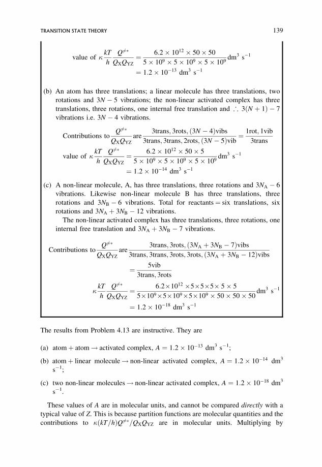
value of �kT
h
Q 6¼�
QXQYZ
¼ 6:2 1012 50 50
5 109 5 109 5 109dm3 s�1
¼ 1:2 10�13 dm3 s�1
(b) An atom has three translations; a linear molecule has three translations, two
rotations and 3N � 5 vibrations; the non-linear activated complex has three
translations, three rotations, one internal free translation and ; 3ðN þ 1Þ � 7
vibrations i.e. 3N � 4 vibrations.
Contributions toQ 6¼�
QXQYZ
are3trans; 3rots; ð3N � 4Þvibs
3trans; 3trans; 2rots; ð3N � 5Þvib¼ 1rot; 1vib
3trans
value of �kT
h
Q6¼�
QXQYZ
¼ 6:2 1012 50 5
5 109 5 109 5 109dm3 s�1
¼ 1:2 10�14 dm3 s�1
(c) A non-linear molecule, A, has three translations, three rotations and 3NA � 6
vibrations. Likewise non-linear molecule B has three translations, three
rotations and 3NB � 6 vibrations. Total for reactants¼ six translations, six
rotations and 3NA þ 3NB � 12 vibrations.
The non-linear activated complex has three translations, three rotations, one
internal free translation and 3NA þ 3NB � 7 vibrations.
Contributions toQ6¼�
QXQYZ
are3trans; 3rots; ð3NA þ 3NB � 7Þvibs
3trans; 3trans; 3rots; 3rots; ð3NA þ 3NB � 12Þvibs
¼ 5vib
3trans; 3rots
�kT
h
Q6¼�
QXQYZ
¼ 6:21012 555 5 5
510951095109 50 50 50dm3 s�1
¼ 1:2 10�18 dm3 s�1
The results from Problem 4.13 are instructive. They are
(a) atomþ atom! activated complex, A ¼ 1:2 10�13 dm3 s�1;
(b) atomþ linear molecule! non-linear activated complex, A ¼ 1:2 10�14 dm3
s�1;
(c) two non-linear molecules! non-linear activated complex, A ¼ 1:2 10�18 dm3
s�1.
These values of A are in molecular units, and cannot be compared directly with a
typical value of Z. This is because partition functions are molecular quantities and the
contributions to �ðkT=hÞQ6¼�=QXQYZ are in molecular units. Multiplying by
TRANSITION STATE THEORY 139
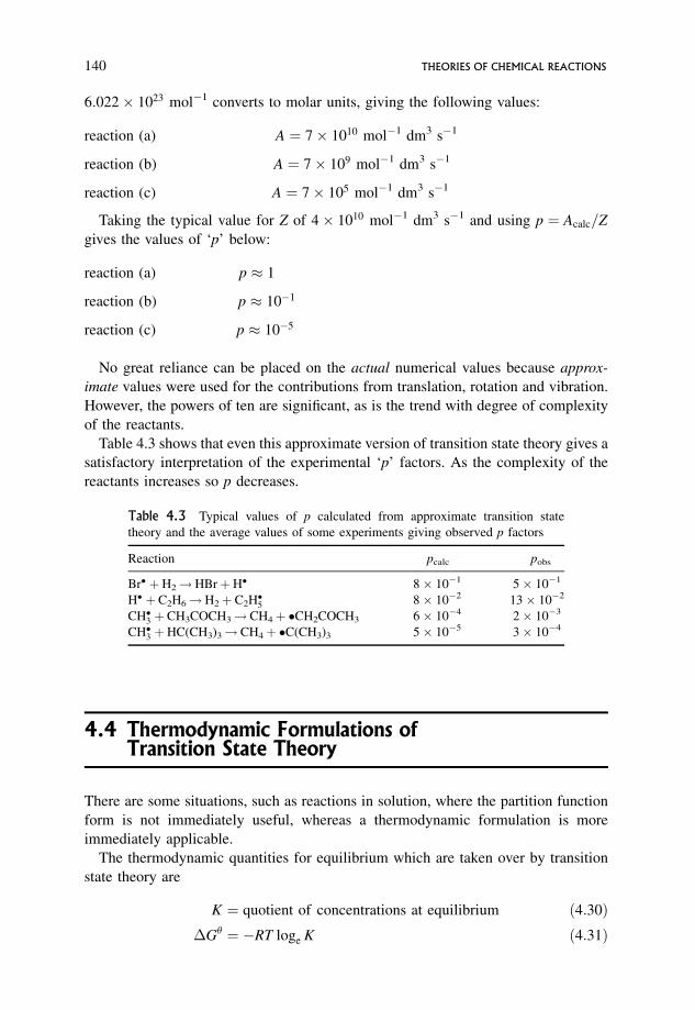
6:022 1023 mol�1 converts to molar units, giving the following values:
reaction (a) A ¼ 7 1010 mol�1 dm3 s�1
reaction (b) A ¼ 7 109 mol�1 dm3 s�1
reaction (c) A ¼ 7 105 mol�1 dm3 s�1
Taking the typical value for Z of 4 1010 mol�1 dm3 s�1 and using p ¼ Acalc=Z
gives the values of ‘p’ below:
reaction (a) p � 1
reaction (b) p � 10�1
reaction (c) p � 10�5
No great reliance can be placed on the actual numerical values because approx-
imate values were used for the contributions from translation, rotation and vibration.
However, the powers of ten are significant, as is the trend with degree of complexity
of the reactants.
Table 4.3 shows that even this approximate version of transition state theory gives a
satisfactory interpretation of the experimental ‘p’ factors. As the complexity of the
reactants increases so p decreases.
4.4 Thermodynamic Formulations ofTransition State Theory
There are some situations, such as reactions in solution, where the partition function
form is not immediately useful, whereas a thermodynamic formulation is more
immediately applicable.
The thermodynamic quantities for equilibrium which are taken over by transition
state theory are
K ¼ quotient of concentrations at equilibrium ð4:30Þ�G ¼ �RT loge K ð4:31Þ
Table 4.3 Typical values of p calculated from approximate transition state
theory and the average values of some experiments giving observed p factors
Reaction pcalc pobs
Br� þH2!HBrþH� 8 10�1 5 10�1
H� þ C2H6!H2þ C2H�5 8 10�2 13 10�2
CH�3 þ CH3COCH3! CH4þ �CH2COCH3 6 10�4 2 10�3
CH�3 þHC(CH3)3! CH4þ �C(CH3)3 5 10�5 3 10�4
140 THEORIES OF CHEMICAL REACTIONS
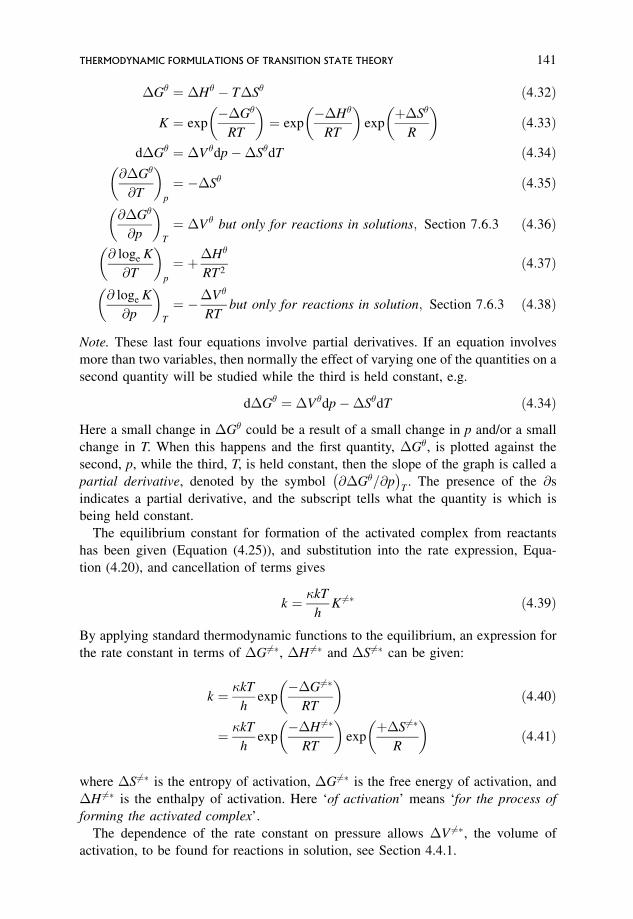
�G ¼ �H � T�S ð4:32Þ
K ¼ exp��G
RT
� �¼ exp
��H
RT
� �exp
þ�S
R
� �ð4:33Þ
d�G ¼ �Vdp��SdT ð4:34Þ@�G
@T
� �p
¼ ��S ð4:35Þ
@�G
@p
� �T
¼ �V but only for reactions in solutions; Section 7:6:3 ð4:36Þ
@ loge K
@T
� �p
¼ þ�H
RT2ð4:37Þ
@ loge K
@p
� �T
¼ ��V
RTbut only for reactions in solution; Section 7:6:3 ð4:38Þ
Note. These last four equations involve partial derivatives. If an equation involves
more than two variables, then normally the effect of varying one of the quantities on a
second quantity will be studied while the third is held constant, e.g.
d�G ¼ �Vdp��SdT ð4:34Þ
Here a small change in �G could be a result of a small change in p and/or a small
change in T. When this happens and the first quantity, �G, is plotted against the
second, p, while the third, T, is held constant, then the slope of the graph is called a
partial derivative, denoted by the symbol @�G=@p� �
T. The presence of the @s
indicates a partial derivative, and the subscript tells what the quantity is which is
being held constant.
The equilibrium constant for formation of the activated complex from reactants
has been given (Equation (4.25)), and substitution into the rate expression, Equa-
tion (4.20), and cancellation of terms gives
k ¼ �kT
hK 6¼� ð4:39Þ
By applying standard thermodynamic functions to the equilibrium, an expression for
the rate constant in terms of �G 6¼�, �H 6¼� and �S6¼� can be given:
k ¼ �kT
hexp
��G 6¼�
RT
� �ð4:40Þ
¼ �kT
hexp
��H 6¼�
RT
� �exp
þ�S 6¼�
R
� �ð4:41Þ
where �S6¼� is the entropy of activation, �G6¼� is the free energy of activation, and
�H 6¼� is the enthalpy of activation. Here ‘of activation’ means ‘for the process of
forming the activated complex’.
The dependence of the rate constant on pressure allows �V 6¼�, the volume of
activation, to be found for reactions in solution, see Section 4.4.1.
THERMODYNAMIC FORMULATIONS OF TRANSITION STATE THEORY 141
The thermodynamic functions for activation are standard values, with the standard
state normally taken to be unit concentration. These all have one term missing, see
Sections 4.3.3 and 4.3.4.
4.4.1 Determination of thermodynamic functions for activation
Detailed calculations using partition functions, calculated from spectroscopic data for
reactants and the PE surface for the activated complex, allows K 6¼�, �G6¼�, �H 6¼�,�S6¼� and �V 6¼� to be found. Experimental data can give experimental values to
compare direct with the theoretical ones. Equation (4.41) gives
loge
k
T¼ loge
�k
hþ�S6¼�
R��H 6¼�
RTð4:42Þ
A plot of logeðk=TÞ versus 1=T has slope ¼ ��H 6¼�=R and intercept ¼logeð�k=hÞ þ�S6¼�=R. Since �kT=h is known, � being generally taken to be unity,
�S6¼� can be found.
Similarly, the effect of pressure on the rate constant gives �V 6¼� for reactions in
solution. Equation (4.40) gives
@ loge k
@p
� �T
¼ � 1
RT
@�G 6¼�
@p
� �T
¼ ��V 6¼�
RTð4:43Þ
A plot of loge k versus p has slope ¼ ��V 6¼�=RT .
Note: the partial derivatives here, @ loge k=@pð ÞT and @�G 6¼�= @p� �
Twhere k varies
with p at constant T, and �G6¼� varies with p at constant T.
4.4.2 Comparison of collision theory, the partition function form
and the thermodynamic form of transition state theory
Worked Problem 4.14
Question. Write out the equations for the statistical mechanical form, the
thermodynamic form, collision theory and the Arrhenius theory. What are the
equivalent terms?
Answer.
k ¼ �kT
h
Q 6¼�
QXQYZ
exp�E0
RT
� �ð4:20Þ
142 THEORIES OF CHEMICAL REACTIONS
k ¼ �kT
hexp
��H 6¼�
RT
� �exp
þ�S 6¼�
R
� �ð4:41Þ
k ¼ pZ exp�EA
RT
� �ð4:29Þ
k ¼ A exp�EA
RT
� �ð4:1Þ
If the exponential terms E0=RT , �H 6¼�=RT and EA=RT can be correlated with
each other and if �kT=h is related to Z, then A; pZ; �ðkT=hÞQ6¼�=QXQYZ and
ð�kT=hÞ exp þ�S6¼�=R� �
can be correlated, while p, Q6¼�=QXQYZ and �S 6¼�=R are
related to each other.
Since �kT=h is a constant for a given T, A factors explicitly reflect any trend in
�S6¼� with reactant type (see Table 4.4). For these reactions �S6¼� is taken to reflect
the complexity of reacting molecules and activated complexes. Log10 A and �S6¼�
parallel each other, and decrease as the complexity of the reacting molecules
increases.
Worked Problem 4.15
Question. Comment on the results given in Table 4.4. Plot log10 A versus �S6¼�
and comment.
Answer. As molecular complexity increases, �S 6¼� becomes increasingly more
negative and so expð�S6¼�
RÞ becomes increasingly smaller. This correlates with the A
factors quoted.
A graph of log10 A versus �S6¼� is approximately linear (Figure 4.28). This is
expected since the same physical phenomenon manifests itself in each.
However, note the comment in the table.
Table 4.4 Values of log10 A and �S6¼� associated with Figure 4.28
Reaction T/K log10A
mol�1 dm3 s�1
� ��S6¼�/J K�1 mol�1
H� þD2!HDþD� 600 10.7 �62
OH� þ CH4!H2Oþ CH�3 300 9.5 �80
CH�3 þH2! CH4þH� 600 9.5 �85
CH�3 þ C2H6! CH4þ C2H�5 650 9.3 �90
CH�3 þ (CH3)3CH! CH4þ (CH3)3C� 650 8.5 �105
Ideally this data should be collected at the same temperature for all reactions. Not doing so
increases the scatter in the graph.
THERMODYNAMIC FORMULATIONS OF TRANSITION STATE THEORY 143
4.4.3 Typical approximate values of contributions entering
the sign and magnitude of �S 6¼�
Translational terms are based here on a standard concentration of 1 mol dm�3. All
values depend somewhat on temperature.
Translation: ca 125 to 175 J mol�1 K�1
ca 40 to 60 J mol�1 K�1 per degree of freedom
Rotation: ca 50 to 100 J mol�1 K�1 for linear molecules
ca 75 to 150 J mol�1 K�1 for non-linear molecules
ca 25 to 50 J mol�1 K�1 per degree of freedom
Vibration: per normal mode: from nearly zero, for high frequencies
at normal temperatures, up to ca 15 J mol�1 K�1 for low
frequencies at higher temperatures
Worked Problem 4.16
Question. Assuming a contribution to �S6¼� of
50 J mol�1 K�1 for each of three translational degrees of freedom,
40 J mol�1 K�1 per each rotational degree of freedom and
10 J mol�1 K�1 per normal mode of vibration;
log10 (A/mol–1 dm3 s–1)
∆S≠*/J K–1 mol–1
8
9
10
11
_60_80_100
Figure 4.28 A graph of log10 A versus �S6¼�
144 THEORIES OF CHEMICAL REACTIONS
calculate �S6¼� for the following reaction,
Aþ B �!ðA----BÞ6¼ ! products
A, B and the activated complex are non-linear with NA, NB and NAþ NB atoms
respectively.
Answer.
A has three translations, three rotations and 3NA� 6 vibrations.
B has three translations, three rotations and 3NB� 6 vibrations.
(A----B)6¼ has three translations, three rotations, one internal free translation and
(3NAþ 3NB� 7) vibrations. Reactants have a total of six translations, six rotations
and (3NAþ 3NB� 12) vibrations. The activated complex has a total of three
translations, three rotations, one internal free translation and (3NAþ 3NB� 7)
vibrations.
On forming the activated complex, we lose three translations and three rotations
and gain 5 vibrations. The activated complex gains one internal free translation, but
this has already been taken care of in the derivation of the rate expression and does
not appear in the exp þ�S6¼�=R� �
term. Quantifying this gives translation, lose 150
J mol�1 K�1; rotation, lose 120 J mol�1 K�1; vibration, gain 50 J mol�1 K�1; net
loss is 220 J mol�1 K�1.
Hence for this reaction using the rough and ready magnitudes quoted,
�S6¼� ¼ �220 J mol�1 K�1. Since �S6¼�=R correlates with the p factor the large
negative value for �S6¼� corresponds to a low p factor.
This is, of course, only a very descriptive calculation.
4.5 Unimolecular Theory
In unimolecular reactions one single reactant molecule passes into the activated
complex and reacts. Experimental observations show that, within any given experi-
ment, unimolecular reactions are strictly first order irrespective of the initial
concentration or pressure (Figure 4.29).
At high pressures the observed first order rate constant is strictly independent of
pressure, but if experiments are carried out at low or intermediate pressures then the
first order rate constant depends on pressure, and the reaction moves from strict first
order kinetics at high pressures to second order at low pressures. At pressures
intermediate between these two limits, the reaction shows complex kinetics with no
simple order. This requires explanation, see below and Problem 4.17.
When studying reactions in the gas phase, the kinetics have often been studied by
following the change in pressure with time. This is particularly so with unimolecular
reactions, and kineticists tend to discuss the experimental results for these reactions in
UNIMOLECULAR THEORY 145
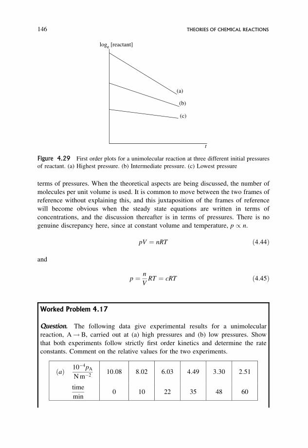
terms of pressures. When the theoretical aspects are being discussed, the number of
molecules per unit volume is used. It is common to move between the two frames of
reference without explaining this, and this juxtaposition of the frames of reference
will become obvious when the steady state equations are written in terms of
concentrations, and the discussion thereafter is in terms of pressures. There is no
genuine discrepancy here, since at constant volume and temperature, p / n.
pV ¼ nRT ð4:44Þ
and
p ¼ n
VRT ¼ cRT ð4:45Þ
Worked Problem 4.17
Question. The following data give experimental results for a unimolecular
reaction, A! B, carried out at (a) high pressures and (b) low pressures. Show
that both experiments follow strictly first order kinetics and determine the rate
constants. Comment on the relative values for the two experiments.
ðaÞ 10�4pA
N m�210:08 8:02 6:03 4:49 3:30 2:51
time
min0 10 22 35 48 60
(a)
loge [reactant]
(b)
(c)
t
Figure 4.29 First order plots for a unimolecular reaction at three different initial pressures
of reactant. (a) Highest pressure. (b) Intermediate pressure. (c) Lowest pressure
146 THEORIES OF CHEMICAL REACTIONS
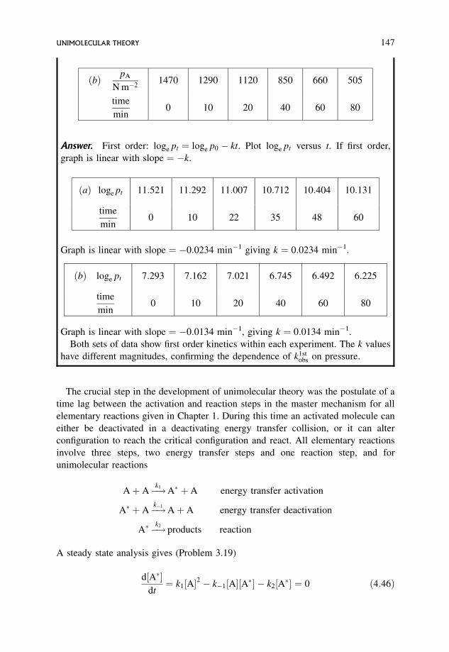
ðbÞ pA
N m�21470 1290 1120 850 660 505
time
min0 10 20 40 60 80
Answer. First order: loge pt ¼ loge p0 � kt. Plot loge pt versus t. If first order,
graph is linear with slope ¼ �k.
ðaÞ loge pt 11:521 11:292 11:007 10:712 10:404 10:131
time
min0 10 22 35 48 60
Graph is linear with slope ¼ �0:0234 min�1 giving k ¼ 0:0234 min�1.
ðbÞ loge pt 7:293 7:162 7:021 6:745 6:492 6:225
time
min0 10 20 40 60 80
Graph is linear with slope ¼ �0:0134 min�1, giving k ¼ 0:0134 min�1.
Both sets of data show first order kinetics within each experiment. The k values
have different magnitudes, confirming the dependence of k1stobs on pressure.
The crucial step in the development of unimolecular theory was the postulate of a
time lag between the activation and reaction steps in the master mechanism for all
elementary reactions given in Chapter 1. During this time an activated molecule can
either be deactivated in a deactivating energy transfer collision, or it can alter
configuration to reach the critical configuration and react. All elementary reactions
involve three steps, two energy transfer steps and one reaction step, and for
unimolecular reactions
Aþ A�!k1A� þ A energy transfer activation
A� þ A�!k�1Aþ A energy transfer deactivation
A� �!k2products reaction
A steady state analysis gives (Problem 3.19)
d½A��dt¼ k1½A�2 � k�1½A�½A�� � k2½A�� ¼ 0 ð4:46Þ
UNIMOLECULAR THEORY 147
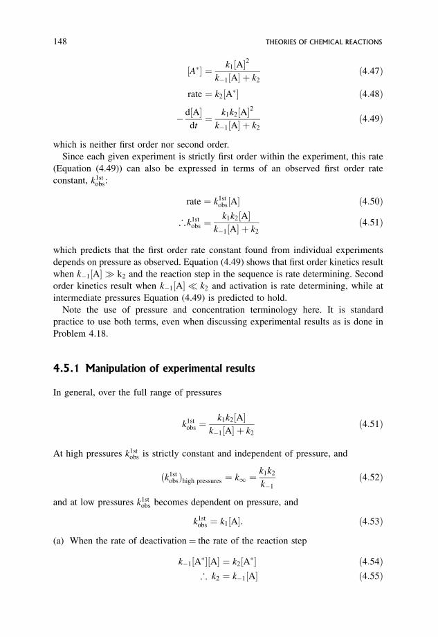
½A�� ¼ k1½A�2
k�1½A� þ k2
ð4:47Þ
rate ¼ k2½A�� ð4:48Þ
� d½A�dt¼ k1k2½A�2
k�1½A� þ k2
ð4:49Þ
which is neither first order nor second order.
Since each given experiment is strictly first order within the experiment, this rate
(Equation (4.49)) can also be expressed in terms of an observed first order rate
constant, k1stobs:
rate ¼ k1stobs½A� ð4:50Þ
;k1stobs ¼
k1k2½A�k�1½A� þ k2
ð4:51Þ
which predicts that the first order rate constant found from individual experiments
depends on pressure as observed. Equation (4.49) shows that first order kinetics result
when k�1½A� � k2 and the reaction step in the sequence is rate determining. Second
order kinetics result when k�1½A� k2 and activation is rate determining, while at
intermediate pressures Equation (4.49) is predicted to hold.
Note the use of pressure and concentration terminology here. It is standard
practice to use both terms, even when discussing experimental results as is done in
Problem 4.18.
4.5.1 Manipulation of experimental results
In general, over the full range of pressures
k1stobs ¼
k1k2½A�k�1½A� þ k2
ð4:51Þ
At high pressures k1stobs is strictly constant and independent of pressure, and
ðk1stobsÞhigh pressures ¼ k1 ¼
k1k2
k�1
ð4:52Þ
and at low pressures k1stobs becomes dependent on pressure, and
k1stobs ¼ k1½A�: ð4:53Þ
(a) When the rate of deactivation¼ the rate of the reaction step
k�1½A��½A� ¼ k2½A�� ð4:54Þ; k2 ¼ k�1½A� ð4:55Þ
148 THEORIES OF CHEMICAL REACTIONS
When this condition is met, and only then, Equation (4.51) reduces to
k1stobs ¼
k1k2
2k�1
¼ k12
ð4:56Þ
The pressure at which the observed first order rate constant has fallen to one-half of
its high pressure value corresponds to
k2 ¼ k�1½A�1=2 ð4:57Þ
or put otherwise
½A�1=2 ¼k2
k�1
ð4:58Þ
[A]1/2 can be found from experiment, and if k�1 is taken to be �Z, then
k2 ¼ �Z½A�1=2 ð4:59Þ
where Z is the collision number and � is the collision efficiency.
Once k2 is found from experiment in this way, then k1 can be found from the
experimental value of k1:
k1 ¼k1k�1
k2
¼ k1�Z
k2
ð4:60Þ
(b) The experimental results can be presented graphically in a plot of 1=k1stobs versus
1=½A�. Rearrangement of Equation (4.51) gives
1
k1stobs
¼ k�1
k1k2
þ 1
k1½A�ð4:61Þ
This will only be linear if k1, k�1 and k2 are constants, in which case the graph will
have slope ¼ 1=k1 and intercept ¼ k�1=k1k2. This gives an alternative route to k2,
again provided k�1 is known.
If, however, k1 and k2 are not single valued, then the graph will be a curve.
Experimental data do, in fact, demonstrate conclusively that the graph is a curve.
Section 4.5.2 discusses the physical significance of the constancy or otherwise of
these rate constants.
Worked Problem 4.18
Question. The decomposition of cyclopropane to propene is a unimolecular
reaction. It can be studied over a range of pressures. The following data gives
values of k1stobs over a range of concentrations. Plot k1st
obs versus concentration and
comment on the shape of the graph.
UNIMOLECULAR THEORY 149
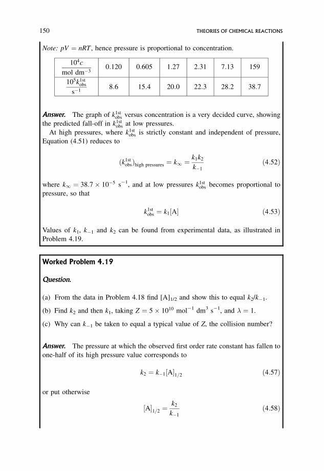
Note: pV ¼ nRT , hence pressure is proportional to concentration.
104c
mol dm�30:120 0:605 1:27 2:31 7:13 159
105k1stobs
s�18:6 15:4 20:0 22:3 28:2 38:7
Answer. The graph of k1stobs versus concentration is a very decided curve, showing
the predicted fall-off in k1stobs at low pressures.
At high pressures, where k1stobs is strictly constant and independent of pressure,
Equation (4.51) reduces to
ðk1stobsÞhigh pressures ¼ k1 ¼
k1k2
k�1
ð4:52Þ
where k1 ¼ 38:7 10�5 s�1, and at low pressures k1stobs becomes proportional to
pressure, so that
k1stobs ¼ k1½A� ð4:53Þ
Values of k1, k�1 and k2 can be found from experimental data, as illustrated in
Problem 4.19.
Worked Problem 4.19
Question.
(a) From the data in Problem 4.18 find [A]1/2 and show this to equal k2/k�1.
(b) Find k2 and then k1, taking Z ¼ 5 1010 mol�1 dm3 s�1, and � ¼ 1.
(c) Why can k�1 be taken to equal a typical value of Z, the collision number?
Answer. The pressure at which the observed first order rate constant has fallen to
one-half of its high pressure value corresponds to
k2 ¼ k�1½A�1=2 ð4:57Þ
or put otherwise
½A�1=2 ¼k2
k�1
ð4:58Þ
150 THEORIES OF CHEMICAL REACTIONS
If k�1 is taken to be �Z, then
k2 ¼ �Z½A�1=2 ð4:59Þ
From Problem 4.18 k1 ¼ 38:7 10�5 s�1 and ½A�1=2 ¼ 1:2 10�4 mol dm�3,
giving k2 ¼ 5 1010 mol�1 dm3 s�1 1:2 10�4 mol dm�3 ¼ 6 106 s�1.
Equation (4.52) can be rearranged to give
k1 ¼k1k�1
k2
¼ k1�Z
k2
¼ 38:7 10�5 s�1 5 1010 mol�1 dm3 s�1
6 106 s�1
¼ 3:2 mol�1 dm3 s�1
where � ¼ 1.
It is likely that only one collision is needed to deactivate an activated molecule,
and so k�1 can be equated to the collision number.
4.5.2 Physical significance of the constancy or
otherwise of k1, k�1 and k2
The analysis of the experimental results given in Problem 4.19 assumes that k1, k�1
and k2 are constants. k1 and k�1 describe the energy transfers of activation and
deactivation. The assumption that these rate constants are single valued means that no
distinction is drawn between the various excited vibrational levels corresponding to
activated molecules. A unique value for k2 implies that a very highly activated
molecule decomposes at the same rate as a molecule with just the critical energy.
Likewise a unique value for k�1 implies that deactivation from a highly excited
molecule occurs at the same rate as that for a molecule with just the critical energy.
These assumptions can be tested by experimental data in the following way.
Equation (4.51) can be rearranged to give
1
k1stobs
¼ k�1
k1k2
þ 1
k1½A�ð4:61Þ
If k1, k�1 and k2 are constants, i.e. are independent of the energy levels involved, see
Sections 4.5.5, 4.5.7 and 4.5.10, the graph of 1=k1stobs versus 1/[A] should be linear with
slope¼ 1/k1 and intercept¼ k�1=k1k2. This would provide an alternative route to k1
and k2, provided an assumed value is given to k�1. If the graph is not linear, this
means that some or all of the rate constants are not single valued. Experiments on
energy transfer and molecular beams indicate that it is a reasonable approximation to
assume that k�1 is single valued, but that it is incorrect to assume k1 and k2 to be
single valued. Problem 4.20 illustrates this and allows a decision to be made.
UNIMOLECULAR THEORY 151
Worked Problem 4.20
Question. Take the values of k1stobs and [A] given in Problem 4.18 and use them to
decide whether k1, k�1 and k2 are constants.
Answer.
10�4 1½A�
mol�1 dm�38:3 1:65 0:79 0:433 0:140 0:006
10�3 1k1st
obs
s11:6 6:5 5:0 4:5 3:55 2:58
Figure 4.30 gives a plot of 1/k1stobs versus 1/[A], and demonstrates conclusively
that at least one of the rate constants is not single valued.
4.5.3 Physical significance of the critical energy in
unimolecular reactions
In bimolecular reactions where two molecules with at least the critical energy
between them move into the critical configuration and react, the critical energy is
assumed to have been accumulated in the energy of relative translational motion
along the line of centres of the colliding molecules. But is this a sensible criterion for
the critical energy in a unimolecular reaction, where the single activated molecule
moves into the critical configuration and reacts? The answer is an unambiguous ‘no’.
All unimolecular theories consider vibrational energy to be the principal factor
12
10
8
6
4
2
0 1 2 3 4 5 6 7 8
110_3 ×
1stobsk
10_4 × 1
[A]
mol_1 dm3
s
Figure 4.30 Graph of 1=k1stobs versus 1/[A] showing departure from linearity
152 THEORIES OF CHEMICAL REACTIONS

contributing to the critical energy which enables the activated molecule to split up. It
is easily visualized that the over-extension of a bond or bond angle as a result of
vigorous vibration of the molecule as a whole could result in reaction.
Worked Problem 4.21
Question. Why is rotational energy not considered to be as important as vibrational
energy in a unimolecular reaction? In what circumstances might it be important?
Answer. The maximum number of rotational modes is three. In nearly all
polyatomic molecules there are considerably more vibrational modes, e.g. CH4
has nine. It is only with very small molecules that rotation might play a significant
role, e.g. in the decompositions of O3 and N2O. The non-linear O3 has three
rotations and three vibrations, while the linear N2O has two rotations and four
vibrations.
4.5.4 Physical significance of the rate constants k1, k�1 and k2
These can be described in terms of a simple model and a complex model. For both, it
is assumed that the critical energy corresponds to vibrational energy.
4.5.5 The simple model: that of Lindemann
� The rate constant for activation, k1. There is one rate constant describing activation
to all vibrational levels above the critical energy, "0, so there is no discrimination
between these high energy levels. The critical energy is assumed to be accumulated
in one vibrational mode.
This model makes a simple distinction between molecules without the critical
energy, and those with at least the critical energy, i.e. activated or energized
molecules. It takes no account of the fact that activated molecules actually do have
vibrational levels of differing energies; and that the question ‘is it as easy to activate a
molecule to the first vibrational level above the critical as it is to activate the molecule
to a high vibrational level?’ could be asked. Intuitively this seems unlikely. As shown
in the analysis of Problem 4.20 this assumption is unlikely to be correct.
� The rate constant for deactivation, k�1. In all the major theories k�1 takes a unique
value and describes deactivation from all energy levels above the critical to any
level below the critical. The magnitude is often taken to be �Z, where Z is the
collision number and � is a collision efficiency that lies between zero and unity.
Again this implies that no distinction is made between differing energy levels
above the critical. Energy transfer experiments show that this is a better approxima-
tion than the corresponding activation assumption, in so far as one collision is often
UNIMOLECULAR THEORY 153
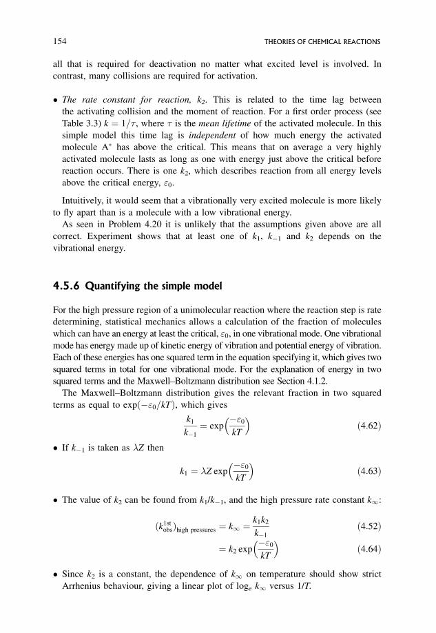
all that is required for deactivation no matter what excited level is involved. In
contrast, many collisions are required for activation.
� The rate constant for reaction, k2. This is related to the time lag between
the activating collision and the moment of reaction. For a first order process (see
Table 3.3) k ¼ 1= , where is the mean lifetime of the activated molecule. In this
simple model this time lag is independent of how much energy the activated
molecule A� has above the critical. This means that on average a very highly
activated molecule lasts as long as one with energy just above the critical before
reaction occurs. There is one k2, which describes reaction from all energy levels
above the critical energy, "0.
Intuitively, it would seem that a vibrationally very excited molecule is more likely
to fly apart than is a molecule with a low vibrational energy.
As seen in Problem 4.20 it is unlikely that the assumptions given above are all
correct. Experiment shows that at least one of k1, k�1 and k2 depends on the
vibrational energy.
4.5.6 Quantifying the simple model
For the high pressure region of a unimolecular reaction where the reaction step is rate
determining, statistical mechanics allows a calculation of the fraction of molecules
which can have an energy at least the critical, "0, in one vibrational mode. One vibrational
mode has energy made up of kinetic energy of vibration and potential energy of vibration.
Each of these energies has one squared term in the equation specifying it, which gives two
squared terms in total for one vibrational mode. For the explanation of energy in two
squared terms and the Maxwell–Boltzmann distribution see Section 4.1.2.
The Maxwell–Boltzmann distribution gives the relevant fraction in two squared
terms as equal to expð�"0=kTÞ, which gives
k1
k�1
¼ exp�"0
kT
� �ð4:62Þ
� If k�1 is taken as �Z then
k1 ¼ �Z exp�"0
kT
� �ð4:63Þ
� The value of k2 can be found from k1/k�1, and the high pressure rate constant k1:
ðk1stobsÞhigh pressures ¼ k1 ¼
k1k2
k�1
ð4:52Þ
¼ k2 exp�"0
kT
� �ð4:64Þ
� Since k2 is a constant, the dependence of k1 on temperature should show strict
Arrhenius behaviour, giving a linear plot of loge k1 versus 1/T.
154 THEORIES OF CHEMICAL REACTIONS

� The dependence of k1stobs on pressure is given as
1
k1stobs
¼ k�1
k1k2
þ 1
k1½A�ð4:61Þ
Using the values of k1, k�1, and k2 found as above the dependence of k1st on
pressure can be found.
When these calculated values were compared with experiment,
� k1(observed)� k1(calculated),
� the falling off of the rate constant (k1stobs)high pressures with decrease in pressure occurs
at a much lower pressure than predicted and
� the graph of 1/k1stobs versus 1/[A] is quite decidedly curved.
These observations show that the simple model is inadequate, even though the
observed effect of temperature on k1 is as predicted.
4.5.7 A more complex model: that of Hinshelwood
� The rate constant for activation, k1. This theory considers a more efficient
activation process to bring the calculated k1 more in line with the observed
value. Energy can be accumulated in s normal modes, generally taken to be
vibrational modes, with the value of s not specified. Likewise, the details of how
the normal modes are involved, the number of modes involved and how the energy
is distributed into the normal modes are not specified. The theory does not consider
how the activated molecule moves into the activated complex. It only states that the
activated molecule which is formed lasts until, by an internal redistribution of
energy among the s modes, the relevant geometrical arrangement of the atoms in
the molecule is that corresponding to reaction.
� The rate constant for deactivation, k�1. This is given as equal to �Z.
� The rate constant for the reaction step, k2. Again k2 is assumed to be a constant,
which does not depend on the energy above the critical value from which any given
activated molecule reacts.
4.5.8 Quantifying Hinshelwood’s theory
Energy is accumulated in s vibrational modes, i.e. in 2s squared terms, and the
Maxwell–Boltzmann distribution gives to a first approximation
k1
k�1
¼ ð"0=kTÞs�1
ðs� 1Þ! expð�"0=kTÞ ð4:65Þ
k1 ¼�Zð"0=kTÞs�1
ðs� 1Þ! expð�"0=kTÞ ð4:66Þ
UNIMOLECULAR THEORY 155
Note: The symbol n! (read as n factorial) means the product of all the positive integers
from 1 to n, e.g. 4! ¼ 4 3 2 1 ¼ 24.
It is important to be aware of the difference in algebraic form between the
Maxwell–Boltzmann distribution for two squared terms (Section 4.1.2) and that for
2s squared terms. Also note well that 2s squared terms are used. This is because one
vibrational mode has two squared terms associated with it, and so if activation energy
is accumulated in s vibrational modes then it will be associated with 2s squared terms.
Physically, it may be easier to visualise energy going into normal modes of vibration
than to think of its going into squared terms (Section 4.1.2).
A calculated value of k1stobs can be found from Equation (4.51), which when
rearranged gives
k1stobs ¼
k2k1=k�1
1þ k2=k�1½A�ð4:67Þ
Substituting from Equation (4.65) for k1/k�1 gives
k1stobs ¼
k2
1þ k2=k�1½A�1
ðs� 1Þ!"0
kT
� �s�1
exp�"0
kT
� �ð4:68Þ
where k2 is single valued and constant, in keeping with the model of assuming that the
lifetime of an activated molecule is independent of how much energy it possesses
above the critical.
This equation requires explicit values of k�1, k2, "0 and s.
A first approximate value of k2 can be found from the pressure at which the
observed first order rate constant has fallen to half the constant high pressure value
(Problem 4.19), and this first approximate value can be used to obtain a first
approximate value for k1. Thereafter k2, "0 and s are found by successive iterations
and best fit of experiment with theory.
The high pressure rate constant obtained when the reaction step in the sequence is
rate determining can be calculated using equation (4.52),
k1 ¼k1k2
k�1
giving
k1 ¼ k2
1
ðs� 1Þ!"0
kT
� �s�1
exp�"0
kT
� �ð4:69Þ
where again best fit values for k2, "0 and s are used. It is found that best fits occur
when s is approximately equal to half the total number of normal modes of vibration.
Even although k2 is a constant this equation predicts a non-linear Arrhenius plot.
156 THEORIES OF CHEMICAL REACTIONS
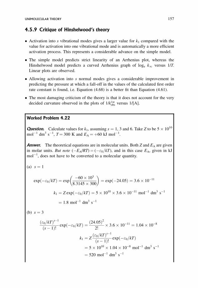
4.5.9 Critique of Hinshelwood’s theory
� Activation into s vibrational modes gives a larger value for k1 compared with the
value for activation into one vibrational mode and is automatically a more efficient
activation process. This represents a considerable advance on the simple model.
� The simple model predicts strict linearity of an Arrhenius plot, whereas the
Hinshelwood model predicts a curved Arrhenius graph of loge k1 versus 1/T.
Linear plots are observed.
� Allowing activation into s normal modes gives a considerable improvement in
predicting the pressure at which a fall-off in the values of the calculated first order
rate constant is found, i.e. Equation (4.68) is a better fit than Equation (4.61).
� The most damaging criticism of the theory is that it does not account for the very
decided curvature observed in the plots of 1/k1stobs versus 1/[A].
Worked Problem 4.22
Question. Calculate values for k1, assuming s ¼ 1, 3 and 6. Take Z to be 5 1010
mol�1 dm3 s�1, T¼ 300 K and EA¼þ60 kJ mol�1.
Answer. The theoretical equations are in molecular units. Both Z and EA are given
in molar units. But note (�EA/RT)¼ (�"0=kT), and in this case EA, given in kJ
mol�1, does not have to be converted to a molecular quantity.
(a) s ¼ 1
expð�"0=kTÞ ¼ exp�60 103
8:3145 300
� �¼ expð�24:05Þ ¼ 3:6 10�11
k1 ¼ Z expð�"0=kTÞ ¼ 5 1010 3:6 10�11 mol�1 dm3 s�1
¼ 1:8 mol�1 dm3 s�1
(b) s ¼ 3
ð"0=kTÞs�1
ðs� 1Þ! expð�"0=kTÞ ¼ ð24:05Þ2
2! 3:6 10�11 ¼ 1:04 10�8
k1 ¼ Zð"0=kTÞs�1
ðs� 1Þ! expð�"0=kTÞ
¼ 5 1010 1:04 10�8 mol�1 dm3 s�1
¼ 520 mol�1 dm3 s�1
UNIMOLECULAR THEORY 157
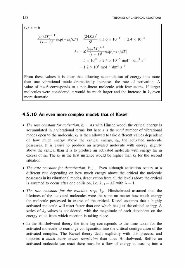
(c) s ¼ 6
ð"0=kTÞs�1
ðs� 1Þ! expð�"0=kTÞ ¼ ð24:05Þ5
5! 3:6 10�11 ¼ 2:4 10�6
k1 ¼ Zð"0=kTÞs�1
ðs� 1Þ! expð�"0=kTÞ
¼ 5 1010 2:4 10�6 mol�1 dm3 s�1
¼ 1:2 105 mol�1 dm3 s�1
From these values it is clear that allowing accumulation of energy into more
than one vibrational mode dramatically increases the rate of activation. A
value of s¼ 6 corresponds to a non-linear molecule with four atoms. If larger
molecules were considered, s would be much larger and the increase in k1 even
more dramatic.
4.5.10 An even more complex model: that of Kassel
� The rate constant for activation, k1. As with Hinshelwood, the critical energy is
accumulated in s vibrational terms, but here s is the total number of vibrational
modes open to the molecule. k1 is then allowed to take different values dependent
on how much energy above the critical energy, "0, the activated molecule
possesses. It is easier to produce an activated molecule with energy slightly
above the critical than it is to produce an activated molecule with energy far in
excess of "0. The k1 in the first instance would be higher than k1 for the second
situation.
� The rate constant for deactivation, k�1. Even although activation occurs at a
different rate depending on how much energy above the critical the molecule
possesses in its vibrational modes, deactivation from all the levels above the critical
is assumed to occur after one collision, i.e. k�1¼ �Z with � ¼ 1.
� The rate constant for the reaction step, k2. Hinshelwood assumed that the
lifetimes of the activated molecules were the same no matter how much energy
the molecule possessed in excess of the critical. Kassel assumes that a highly
activated molecule will react faster than one which has just the critical energy. A
series of k2 values is considered, with the magnitude of each dependent on the
energy value from which reaction is taking place.
� In the Hinshelwood theory the time lag corresponds to the time taken for the
activated molecule to rearrange configuration into the critical configuration of the
activated complex. The Kassel theory deals explicitly with this process, and
imposes a much more severe restriction than does Hinshelwood. Before an
activated molecule can react there must be a flow of energy at least "0 into a
158 THEORIES OF CHEMICAL REACTIONS
critical normal mode. Once this has happened the activated molecule has the
correct distribution of vibrational energy for it to be able to react. The time lag is
the time taken for this to happen.
4.5.11 Critique of the Kassel theory
The derivation is much more complicated than those outlined previously, especially
when the quantum version is considered. Both versions are a vast improvement on the
previous theories, and predict that 1/k1st versus 1/[A] should be a curve, and that the
plot of loge k1 versus 1/T should be linear. Both predictions are verified by
experiment.
More advanced theories continue to make further improvements.
4.5.12 Energy transfer in the activation step
The change over from first order kinetics, when the reaction step is rate determining,
to second order kinetics, when activation is rate determining, depends on the
total pressure, the complexity of the reactant and to a lesser extent on the tempe-
rature.
� Effect of pressure. This has been dealt with in detail on a quantitative basis. But
on a physical basis it is more likely that activation is faster than the reaction step at
high pressures where there is a greater chance of collisions, simply because there
are more molecules around. At low pressures there is less chance of collisions
occurring, again simply because there are fewer molecules around, and so
activation is now slower than reaction.
Remember: activation is bimolecular, while reaction is unimolecular.
� Complexity of the reacting molecule. This reflects the number of atoms in the
molecule, which determines the number of normal modes of vibration open to the
molecule. The critical energy is accumulated in the normal modes of vibration, and
the more complex the molecule the greater the number of modes over which this
energy can be spread. Reaction is a consequence of a bond breaking and only some
of the normal modes will contribute to the behaviour of this bond. The larger
the total number of normal modes, i.e. the greater the complexity, the more
difficult it will be for energy to flow into the critical coordinate, and the greater
will be the time lag between activation and reaction. The reaction step is thus likely
to be rate determining if the molecule is complex and first order kinetics is
observed.
If the molecule is small, there are fewer normal modes over which the critical
energy can be spread, and it is much more likely that the required critical energy
UNIMOLECULAR THEORY 159
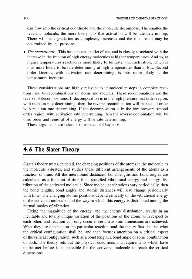
can flow into the critical coordinate and the molecule decompose. The smaller the
reactant molecule, the more likely it is that activation will be rate determining.
There will be a gradation as complexity increases and the final result may be
determined by the pressure.
� The temperature. This has a much smaller effect, and is closely associated with the
increase in the fraction of high energy molecules at higher temperatures. And so, at
higher temperatures reaction is more likely to be faster than activation, which is
thus more likely to be rate determining at high temperatures than at low. Second
order kinetics, with activation rate determining, is thus more likely as the
temperature increases.
These considerations are highly relevant to unimolecular steps in complex reac-
tions, and to recombinations of atoms and radicals. These recombinations are the
reverse of decompositions. If decomposition is in the high pressure first order region,
with reaction rate determining, then the reverse recombination will be second order
with reaction rate determining. If the decomposition is in the low pressure second
order region, with activation rate determining, then the reverse combination will be
third order and removal of energy will be rate determining.
These arguments are relevant to aspects of Chapter 6.
4.6 The Slater Theory
Slater’s theory treats, in detail, the changing positions of the atoms in the molecule as
the molecule vibrates, and studies these different arrangements of the atoms as a
function of time. All the interatomic distances, bond lengths and bond angles are
calculated as a function of time for a specified vibrational energy and energy dis-
tribution of the activated molecule. Since molecular vibrations vary periodically, then
the bond lengths, bond angles and atomic distances will also change periodically
with time. The changing atomic positions depend critically on the vibrational energy
of the activated molecule, and the way in which this energy is distributed among the
normal modes of vibration.
Fixing the magnitude of the energy, and the energy distribution, results in an
inevitable and totally unique variation of the positions of the atoms with respect to
each other, and reaction can only occur if certain atomic dimensions are achieved.
What they are depends on the particular reaction, and the theory first decides what
the critical configuration shall be, and then focuses attention on a critical aspect
of the critical configuration, such as a bond length, a bond angle or some combination
of both. The theory sets out the physical conditions and requirements which have
to be met before it is posssible for the activated molecule to reach the critical
dimensions.
160 THEORIES OF CHEMICAL REACTIONS
Figure 4.31 shows the sine waves for the three normal modes of vibration for the
linear N2O molecule. For the unimolecular decomposition N2O!N2þO� it is
assumed that reaction occurs with the breaking of the N–O bond after it reaches a
certain critical extension. The diagram shows the summing of these three sine waves
and the effect which that has on the extension of the N–O bond with time. The
diagram shows the value of the critical extension which must be reached before the
bond will break. The vibrational energy, and the distribution of this energy among the
normal modes can be seen to be such that the bond does reach the critical value, and
breaks.
The average number of times per unit time that the combination of sine waves,
calculated for the summed normal modes, exceeds the critical extension can be found,
and this gives a value for the first order high pressure rate constant.
Slater’s theory assumes that the normal modes behave as harmonic oscillators,
which requires that there be no flow of energy between the normal modes once the
molecule is suitably activated, and so the energy distribution remains fixed between
collisions. But spectroscopy shows that energy can flow around a molecule, and
allowing for such a flow between collisions vastly improves the theory. Like Kassel’s
theory a fully quantum theory would be superior.
The equation for the high pressure rate constant predicts strict Arrhenius behaviour,
and also a non-linear plot for 1/kobs versus 1/[A], both in agreement with experiment.
However, the beauty of Slater’s theory is that it gives a very clear description of the
process of reaction, which is easy to visualize; that is, ‘the molecule splits up if some
bond(s), bond angle(s) or a combination of both is extended too far’.
N _ Odistance
criticalvalue q0
timebendingsymmetric stretchasymmetric stretchactual motion: sum of all three
Figure 4.31 Summing of normal modes of vibration for N2O
THE SLATER THEORY 161
Further reading
Laidler K.J., Chemical Kinetics, 3rd edn, Harper and Row, New York, 1987.
Laidler K.J. and Meiser J.H., Physical Chemistry, 3rd edn, Houghton Mifflin, New
York, 1999.
Alberty R.A. and Silbey R.J., Physical Chemistry, 2nd edn, Wiley, New York, 1996.
Logan S.R., Fundamentals of Chemical Kinetics, Addison-Wesley, Reading, MA,
1996.
* Nicholas J., Chemical Kinetics, Harper and Row, New York, 1976.
* Wilkinson F., Chemical Kinetics and Reaction Mechanisms, Van Nostrand
Reinhold, New York, 1980.
Robson Wright M., Fundamental Chemical Kinetics, Horwood, Chichester, 1999.
* Laidler K.J., Theories of Chemical Reaction Rates, McGraw-Hill, New York, 1969.
* Glasstone S., Laidler K.J. and Eyring H., Theory of Rate Processes, McGraw-Hill,
New York, 1941.
* Out of print, but should be in university libraries.
Further problems
1. Find the change in the number of degrees of freedom of each type on forming the
activated complex for the following reactions:
� atomþ non-linear molecule to non-linear AC
� linear moleculeþ non-linear molecule to non-linear AC
� two linear molecules to linear AC
� two linear molecules to non-linear AC
� non-linear molecule to non-linear AC.
2. How can �H 6¼� and �S6¼� be found for a gas phase reaction? Why is it that a
�V 6¼� value cannot be found for gas phase reactions?
3. Use transition state theory to calculate approximate �S6¼� values for the following
reactions:
Br� þ H2 ! HBrþ H�
CH�3 þ H2 ! CH4 þ H�
F2 þ ClO�2 ! FClO2 þ F�
C4H6 þ C2H4 ! cyclo� C6H10
Comment on the values obtained.
162 THEORIES OF CHEMICAL REACTIONS
The following are rough values for the contributions to the entropy for
translation: 50 J mol�1 K�1 per degree of freedom
rotation: 40 J mol�1 K�1 per degree of freedom
vibration: 10 J mol�1 K�1 per degree of freedom.
4. Taking the collision diameter to be 400 pm, calculate the collision number, Z, for
collisions between the molecules CH2����CH–CH����CH2 and CH2����CH–CHO at
500 K, and from this find the pre-exponential factor, A.
The following are rough values for the contributions to the entropy from
translation: 40 J mol�1 K�1 per degree of freedom
rotation: 25 J mol�1 K�1 per degree of freedom
vibration: 10 J mol�1 K�1 per degree of freedom.
Using this, make a rough estimate of the transition state theory pre-exponential
factor.
(The experimental A factor¼ 1:6 106 mol�1 dm3 s�1.)
5. Use the following data for a unimolecular decomposition to determine k1 and k2
which appear in the simple Lindemann mechanism; assume that k�1 has a value of
5:0 1010 mol�1 dm3 s�1. From this determine the mean lifetime of the activated
molecule. Comment on the results.
(Proceed by plotting 1/k1stobs versus 1/[A].)
106½A�mol dm�3
10 15 20 40
k1stobs
s�10:333 0:391 0:426 0:495
The following values extend the data to higher concentrations:
106½A�mol dm�3
100 200 400
k1stobs
s�10:625 0:781 0:952
Comment on the plot of 1/kobs versus 1/[A] which is obtained if all the values from
both tables are included.
FURTHER PROBLEMS 163
6. Predict the temperature dependence of A for the bimolecular reactions given in
question 3.
Br� þ H2 ! HBrþ H�
CH�3 þ H2 ! CH4 þ H�
F2 þ ClO�2 ! FClO2 þ F�
C4H6 þ C2H4 ! cyclo-C6H10
(a) the translational partition function for each degree of freedom is proportional to
T1/2;
(b) the rotational partition function for each degree of freedom is proportional to T1/2;
(c) the vibrational partition function for each degree of freedom is independent of
temperature at low temperatures, but is proportional to T1 at high temperatures.
7. The following are values of entropies of activation for some unimolecular
reactions, together with values of �S for the overall reaction:
Reaction�S6¼�
J mol�1 K�1
�S
J mol�1 K�1
cyclo-propane! propane 39 29:5
cyclo-butane! 2C2H4 42 146:9
CH2
O
CH2 CH3CHO21 21:8
CH3NC! CH3CN 4 �3:3
cyclo-C4F8 ! 2C2F4 49 172:9
Compare the �S 6¼� values with the corresponding �S, and comment on the
comparisons. Find the �S6¼� values for the reverse reactions, and comment on the
values obtained.
The values of �S given in the table are based on a standard concentration, as
distinct from the normal values based on a standard pressure. This has been done
because the values of �S6¼� are based on a standard concentration.
164 THEORIES OF CHEMICAL REACTIONS
5 Potential Energy Surfaces
The calculation of the PE surface is basically quantum mechanical. Accurate surfaces
are used to show how the topography of the surface affects the ‘reaction unit’ as it
changes configuration across the surface. Predictions can be made, and these can be
tested by molecular beams, spectroscopic techniques and chemiluminescence.
Aims
By the end of this chapter you should be able to
� distinguish between symmetrical, early and late barriers
� correlate the relative distances between atoms in the ‘reaction entity’ at the criticalconfiguration with the type of potential energy surface
� list the properties of early barriers and correlate them with molecular beam results
� list the properties of late barriers and correlate them with molecular beam resultsand
� predict the dominant type of energy present in products and which type ofenergy promotes reaction.
5.1 The Symmetrical Potential Energy Barrier
It is possible to use the 3-D surface with its corresponding 2-D contour diagram and
potential energy profile to discuss the general reaction Aþ BC! ABþ C where A,
AB, BC and C are all polyatomic molecules.
The progress of the reaction unit A----B----C along the reaction coordinate, or
minimum energy path, is given in terms of relative values of rAB and rBC. Figures 5.1
and 5.2 have been given in terms of a symmetrical barrier where the activated
complex lies symmetrically with respect to both the entrance and exit valleys.
An Introduction to Chemical Kinetics. Margaret Robson Wright# 2004 John Wiley & Sons, Ltd. ISBNs: 0-470-09058-8 (hbk) 0-470-09059-6 (pbk)
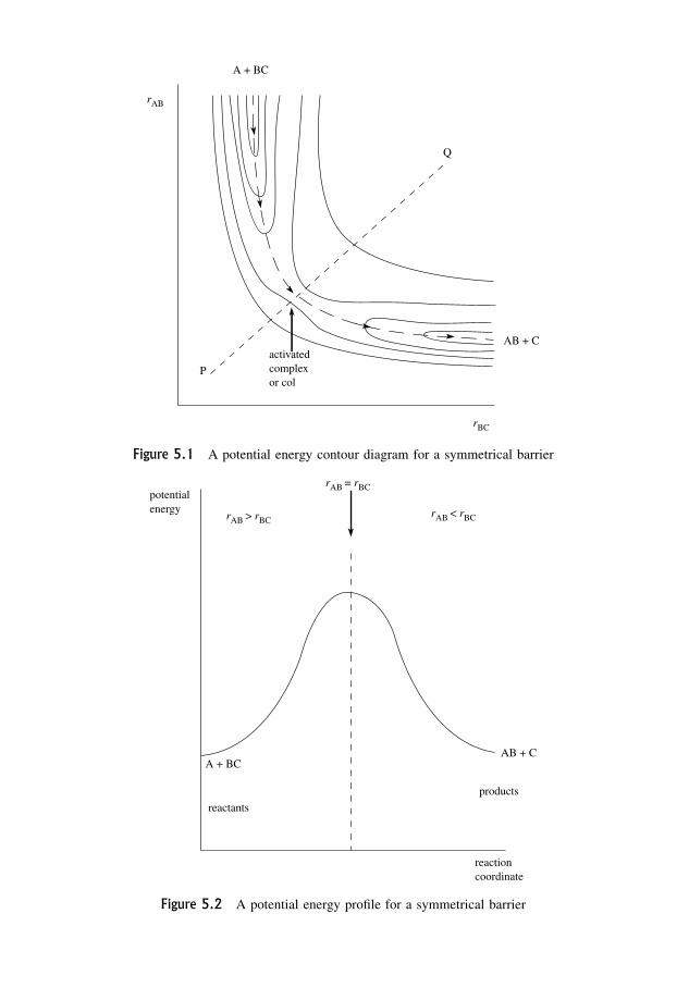
activated complexor col
AB + C
A + BC
rAB
rBC
P
Q
Figure 5.1 A potential energy contour diagram for a symmetrical barrier
A + BC
reactants
reactioncoordinate
products
AB + C
rAB > rBC
rAB = rBC
rAB < rBC
potentialenergy
Figure 5.2 A potential energy profile for a symmetrical barrier
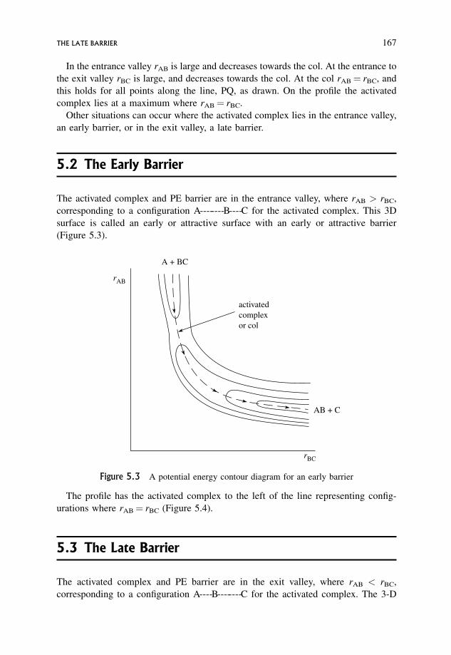
In the entrance valley rAB is large and decreases towards the col. At the entrance to
the exit valley rBC is large, and decreases towards the col. At the col rAB¼ rBC, and
this holds for all points along the line, PQ, as drawn. On the profile the activated
complex lies at a maximum where rAB¼ rBC.
Other situations can occur where the activated complex lies in the entrance valley,
an early barrier, or in the exit valley, a late barrier.
5.2 The Early Barrier
The activated complex and PE barrier are in the entrance valley, where rAB > rBC,
corresponding to a configuration A--------B----C for the activated complex. This 3D
surface is called an early or attractive surface with an early or attractive barrier
(Figure 5.3).
The profile has the activated complex to the left of the line representing config-
urations where rAB¼ rBC (Figure 5.4).
5.3 The Late Barrier
The activated complex and PE barrier are in the exit valley, where rAB < rBC,
corresponding to a configuration A----B--------C for the activated complex. The 3-D
AB + C
A + BC
activatedcomplexor col
rBC
rAB
Figure 5.3 A potential energy contour diagram for an early barrier
THE LATE BARRIER 167
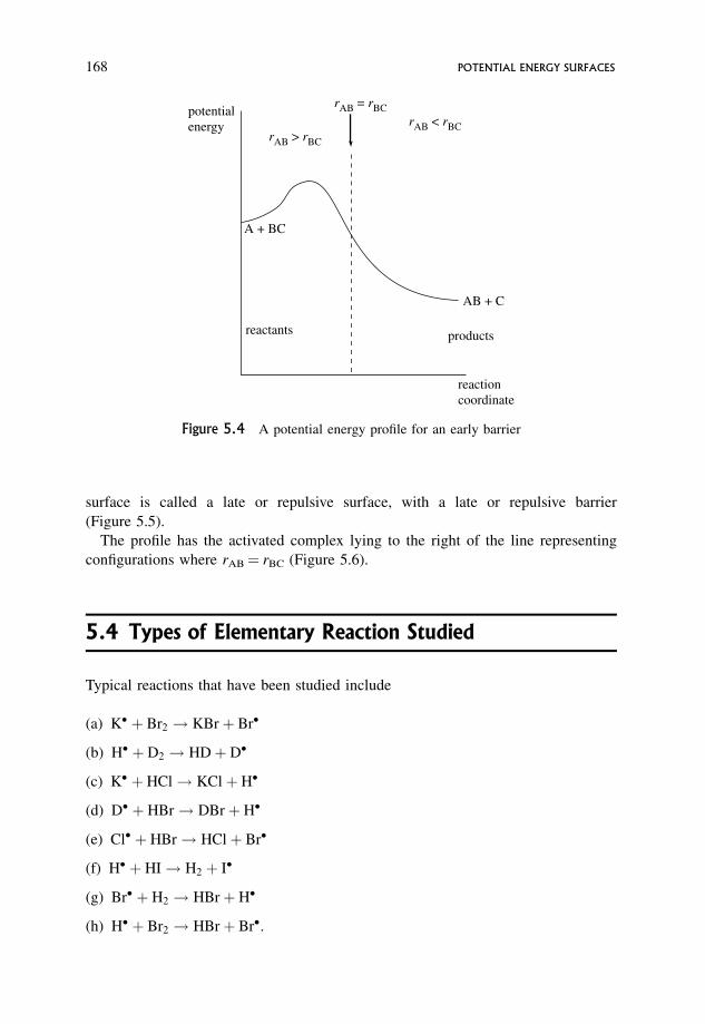
surface is called a late or repulsive surface, with a late or repulsive barrier
(Figure 5.5).
The profile has the activated complex lying to the right of the line representing
configurations where rAB¼ rBC (Figure 5.6).
5.4 Types of Elementary Reaction Studied
Typical reactions that have been studied include
(a) K� þ Br2 ! KBrþ Br�
(b) H� þ D2 ! HDþ D�
(c) K� þ HCl! KClþ H�
(d) D� þ HBr! DBrþ H�
(e) Cl� þ HBr! HClþ Br�
(f) H� þ HI! H2 þ I�
(g) Br� þ H2 ! HBrþ H�
(h) H� þ Br2 ! HBrþ Br�.
rAB > rBC
A + BC
potentialenergy
reactants products
AB + C
reaction coordinate
rAB = rBCrAB < rBC
Figure 5.4 A potential energy profile for an early barrier
168 POTENTIAL ENERGY SURFACES
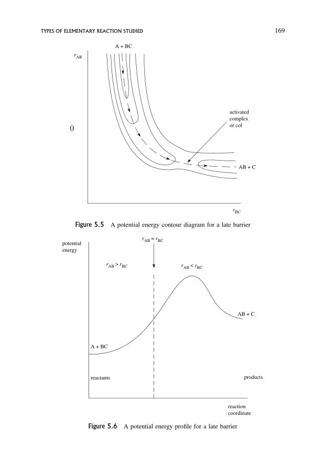
0
rAB
rBC
activatedcomplexor col
AB + C
A + BC
Figure 5.5 A potential energy contour diagram for a late barrier
potentialenergy
reactants products
reactioncoordinate
A + BC
rAB > rBC
rAB = rBC
rAB < rBC
AB + C
Figure 5.6 A potential energy profile for a late barrier
TYPES OF ELEMENTARY REACTION STUDIED 169
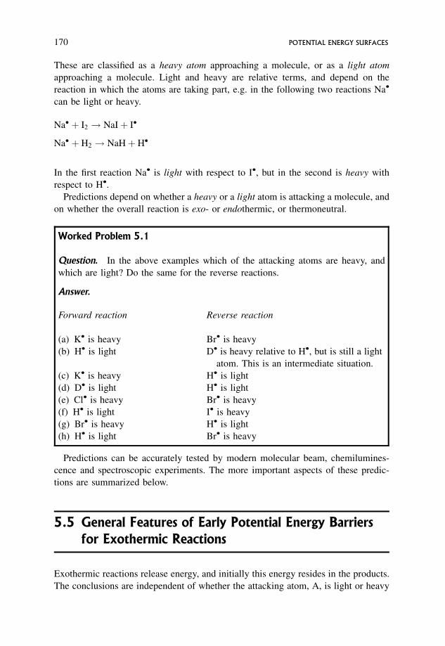
These are classified as a heavy atom approaching a molecule, or as a light atom
approaching a molecule. Light and heavy are relative terms, and depend on the
reaction in which the atoms are taking part, e.g. in the following two reactions Na�
can be light or heavy.
Na� þ I2 ! NaIþ I�
Na� þ H2 ! NaHþ H�
In the first reaction Na� is light with respect to I�, but in the second is heavy with
respect to H�.
Predictions depend on whether a heavy or a light atom is attacking a molecule, and
on whether the overall reaction is exo- or endothermic, or thermoneutral.
Worked Problem 5.1
Question. In the above examples which of the attacking atoms are heavy, and
which are light? Do the same for the reverse reactions.
Answer.
Forward reaction Reverse reaction
(a) K� is heavy Br� is heavy
(b) H� is light D� is heavy relative to H�, but is still a light
atom. This is an intermediate situation.
(c) K� is heavy H� is light
(d) D� is light H� is light
(e) Cl� is heavy Br� is heavy
(f) H� is light I� is heavy
(g) Br� is heavy H� is light
(h) H� is light Br� is heavy
Predictions can be accurately tested by modern molecular beam, chemilumines-
cence and spectroscopic experiments. The more important aspects of these predic-
tions are summarized below.
5.5 General Features of Early Potential Energy Barriers
for Exothermic Reactions
Exothermic reactions release energy, and initially this energy resides in the products.
The conclusions are independent of whether the attacking atom, A, is light or heavy
170 POTENTIAL ENERGY SURFACES
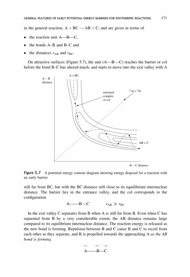
in the general reaction, Aþ BC! ABþ C, and are given in terms of
� the reaction unit A----B----C,
� the bonds A–B and B–C and
� the distances rAB and rBC.
On attractive surfaces (Figure 5.7), the unit (A----B----C) reaches the barrier or col
before the bond B–C has altered much, and starts to move into the exit valley with A
still far from BC, but with the BC distance still close to its equilibrium internuclear
distance. The barrier lies in the entrance valley, and the col corresponds to the
configuration
A--------B----C rAB � rBC
In the exit valley C separates from B when A is still far from B. Even when C has
separated from B by a very considerable extent, the AB distance remains large
compared to its equilibrium internuclear distance. The reaction energy is released as
the new bond is forming. Repulsion between B and C cause B and C to recoil from
each other as they separate, and B is propelled towards the approaching A as the AB
bond is forming.
! !A--------B----C
AB + C
A + BCA -- Bdistance
B -- C distance
activatedcomplexor col
rAB = rBC
Figure 5.7 A potential energy contour diagram showing energy disposal for a reaction with
an early barrier
GENERAL FEATURES OF EARLY POTENTIAL ENERGY BARRIERS FOR EXOTHERMIC REACTIONS 171
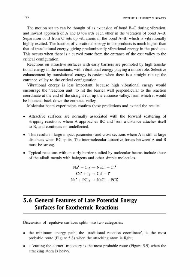
The motion set up can be thought of as extension of bond B–C during vibration,
and inward approach of A and B towards each other in the vibration of bond A–B.
Separation of B from C sets up vibrations in the bond A–B, which is vibrationally
highly excited. The fraction of vibrational energy in the products is much higher than
that of translational energy, giving predominantly vibrational energy in the products.
This occurs when there is a curved route from the entrance of the exit valley to the
critical configuration.
Reactions on attractive surfaces with early barriers are promoted by high transla-
tional energy in the reactants, with vibrational energy playing a minor role. Selective
enhancement by translational energy is easiest when there is a straight run up the
entrance valley to the critical configuration.
Vibrational energy is less important, because high vibrational energy would
encourage the ‘reaction unit’ to hit the barrier wall perpendicular to the reaction
coordinate at the end of the straight run up the entrance valley, from which it would
be bounced back down the entrance valley.
Molecular beam experiments confirm these predictions and extend the results.
� Attractive surfaces are normally associated with the forward scattering of
stripping reactions, where A approaches BC and from a distance attaches itself
to B, and continues on undeflected.
� This results in large impact parameters and cross sections where A is still at large
distances when BC splits. The intermolecular attractive forces between A and B
must be strong.
� Typical reactions with an early barrier studied by molecular beams include those
of the alkali metals with halogens and other simple molecules.
Na� þ Cl2 ! NaClþ Cl�
Cs� þ I2 ! CsIþ I�
Na� þ PCl3 ! NaClþ PCl�2
5.6 General Features of Late Potential Energy
Surfaces for Exothermic Reactions
Discussion of repulsive surfaces splits into two categories:
� the minimum energy path, the ‘traditional reaction coordinate’, is the most
probable route (Figure 5.8) when the attacking atom is light;
� a ‘cutting the corner’ trajectory is the most probable route (Figure 5.9) when the
attacking atom is heavy.
172 POTENTIAL ENERGY SURFACES
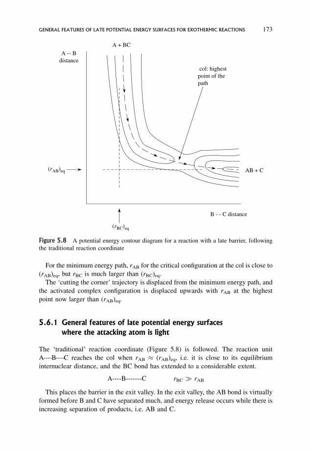
For the minimum energy path, rAB for the critical configuration at the col is close to
(rAB)eq, but rBC is much larger than (rBC)eq.
The ‘cutting the corner’ trajectory is displaced from the minimum energy path, and
the activated complex configuration is displaced upwards with rAB at the highest
point now larger than (rAB)eq.
5.6.1 General features of late potential energy surfaces
where the attacking atom is light
The ‘traditional’ reaction coordinate (Figure 5.8) is followed. The reaction unit
A----B----C reaches the col when rAB � (rAB)eq, i.e. it is close to its equilibrium
internuclear distance, and the BC bond has extended to a considerable extent.
A----B-------C rBC � rAB
This places the barrier in the exit valley. In the exit valley, the AB bond is virtually
formed before B and C have separated much, and energy release occurs while there is
increasing separation of products, i.e. AB and C.
(rBC)eq
(rAB)eq
A -- Bdistance
A + BC
AB + C
B - - C distance
col: highestpoint of the path
Figure 5.8 A potential energy contour diagram for a reaction with a late barrier, following
the traditional reaction coordinate
GENERAL FEATURES OF LATE POTENTIAL ENERGY SURFACES FOR EXOTHERMIC REACTIONS 173
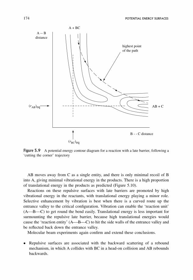
AB moves away from C as a single entity, and there is only minimal recoil of B
into A, giving minimal vibrational energy in the products. There is a high proportion
of translational energy in the products as predicted (Figure 5.10).
Reactions on these repulsive surfaces with late barriers are promoted by high
vibrational energy in the reactants, with translational energy playing a minor role.
Selective enhancement by vibration is best when there is a curved route up the
entrance valley to the critical configuration. Vibration can enable the ‘reaction unit’
(A----B----C) to get round the bend easily. Translational energy is less important for
surmounting the repulsive late barrier, because high translational energies would
cause the ‘reaction entity’ (A----B----C) to hit the side walls of the entrance valley and
be reflected back down the entrance valley.
Molecular beam experiments again confirm and extend these conclusions.
� Repulsive surfaces are associated with the backward scattering of a rebound
mechanism, in which A collides with BC in a head-on collision and AB rebounds
backwards.
(rBC)eq
(rAB)eq
A -- Bdistance
A + BC
AB + C
B - - C distance
highest pointof the path
Figure 5.9 A potential energy contour diagram for a reaction with a late barrier, following a
‘cutting the corner’ trajectory
174 POTENTIAL ENERGY SURFACES
� This results in the small cross sections and small impact parameters expected
when AB has formed as C splits off and separates from B under short range
repulsion.
� Typical reactions studied in this way are between halogen atoms and HCl and HF
Br� þ HCl! HBrþ Cl� Cl� þ HF! HClþ F�
along with the extensively studied reaction
K� þ CH3I! KIþ CH�3
5.6.2 General features of late potential energy surfaces for
exothermic reactions where the attacking atom is heavy
The behaviour for such reactions is very different from that predicted above for
reactions where the attacking atom is light. Both vibration and translation are
activated complexor col
attack by light atom
A + BC
AB + C
B -- C distance
A -- Bdistance
Figure 5.10 A potential energy contour diagram for a light atom attacking in a reaction with
a late barrier, showing energy requirements for reaction and energy disposal in products
GENERAL FEATURES OF LATE POTENTIAL ENERGY SURFACES FOR EXOTHERMIC REACTIONS 175
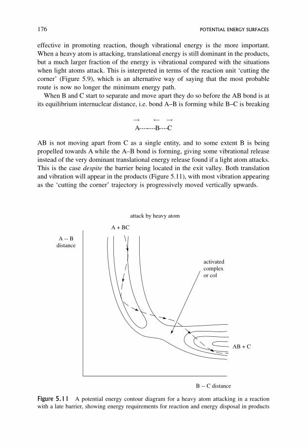
effective in promoting reaction, though vibrational energy is the more important.
When a heavy atom is attacking, translational energy is still dominant in the products,
but a much larger fraction of the energy is vibrational compared with the situations
when light atoms attack. This is interpreted in terms of the reaction unit ‘cutting the
corner’ (Figure 5.9), which is an alternative way of saying that the most probable
route is now no longer the minimum energy path.
When B and C start to separate and move apart they do so before the AB bond is at
its equilibrium internuclear distance, i.e. bond A–B is forming while B–C is breaking
! !A--------B----C
AB is not moving apart from C as a single entity, and to some extent B is being
propelled towards A while the A–B bond is forming, giving some vibrational release
instead of the very dominant translational energy release found if a light atom attacks.
This is the case despite the barrier being located in the exit valley. Both translation
and vibration will appear in the products (Figure 5.11), with most vibration appearing
as the ‘cutting the corner’ trajectory is progressively moved vertically upwards.
activated complexor col
attack by heavy atom
A + BC
AB + C
B -- C distance
A -- Bdistance
Figure 5.11 A potential energy contour diagram for a heavy atom attacking in a reaction
with a late barrier, showing energy requirements for reaction and energy disposal in products
176 POTENTIAL ENERGY SURFACES
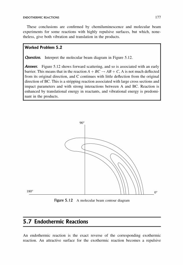
These conclusions are confirmed by chemiluminescence and molecular beam
experiments for some reactions with highly repulsive surfaces, but which, none-
theless, give both vibration and translation in the products.
Worked Problem 5.2
Question. Interpret the molecular beam diagram in Figure 5.12.
Answer. Figure 5.12 shows forward scattering, and so is associated with an early
barrier. This means that in the reaction Aþ BC ! ABþ C, A is not much deflected
from its original direction, and C continues with little deflection from the original
direction of BC. This is a stripping reaction associated with large cross sections and
impact parameters and with strong interactions between A and BC. Reaction is
enhanced by translational energy in reactants, and vibrational energy is predomi-
nant in the products.
5.7 Endothermic Reactions
An endothermic reaction is the exact reverse of the corresponding exothermic
reaction. An attractive surface for the exothermic reaction becomes a repulsive
90°
180° 0°
Figure 5.12 A molecular beam contour diagram
ENDOTHERMIC REACTIONS 177
surface for the endothermic reaction, while the repulsive surface for the exothermic
reaction becomes an attractive surface for the endothermic reaction. Likewise, if an
exothermic reaction is enhanced by translational energy and has predominantly
vibrational energy in the products, then the reverse endothermic reaction will be
promoted by vibrational energy, and will have translational energy dominant in the
products. Recognition of the mass types involved is imperative.
Worked Problem 5.3
Question. List the properties of the endothermic reaction
Aþ BC! ABþ C
corresponding to a reaction on an attractive early exothermic surface.
Answer. The endothermic reaction is the reverse of an exothermic reaction. The
endothermic reaction will have
(a) a repulsive surface with a late barrier, so that the activated complex has a
configuration
A----B--------C
where the bond A–B is close to its equilibrium internuclear distance and bond
B–C has yet to break;
(b) the late barrier means that the bond A–B is formed before the repulsion energy
of B–C is released, so that translational energy is predominant in the products.
Reaction will be enhanced by vibrational energy in reactants. These predictions
are in keeping with the curved route up the entrance valley and the straight run
down the exit valley from the activated complex.
5.8 Reactions with a Collision Complex and a
Potential Energy Well
Sometimes there is a basin or well somewhere along the reaction coordinate on the
surface and a minimum on the profile (Figures 5.13 and 5.14).
If the well is in the entrance valley the ‘reaction unit’ can often need vibrational
energy, but if it is in the exit valley translational energy is often more effective. Such
features are indicative of a collision complex which lasts sufficiently long for many
vibrations and some rotations to occur. The lifetime of a collision complex is long
178 POTENTIAL ENERGY SURFACES
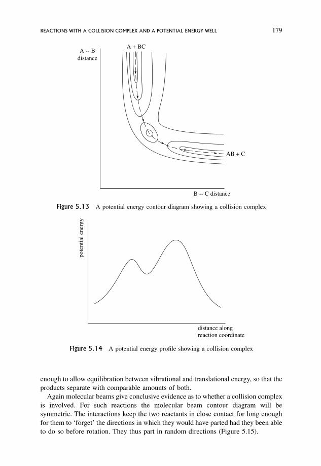
enough to allow equilibration between vibrational and translational energy, so that the
products separate with comparable amounts of both.
Again molecular beams give conclusive evidence as to whether a collision complex
is involved. For such reactions the molecular beam contour diagram will be
symmetric. The interactions keep the two reactants in close contact for long enough
for them to ‘forget’ the directions in which they would have parted had they been able
to do so before rotation. They thus part in random directions (Figure 5.15).
A -- Bdistance
A + BC
AB + C
B -- C distance
Figure 5.13 A potential energy contour diagram showing a collision complex
distance alongreaction coordinate
pote
ntia
l ene
rgy
Figure 5.14 A potential energy profile showing a collision complex
REACTIONS WITH A COLLISION COMPLEX AND A POTENTIAL ENERGY WELL 179
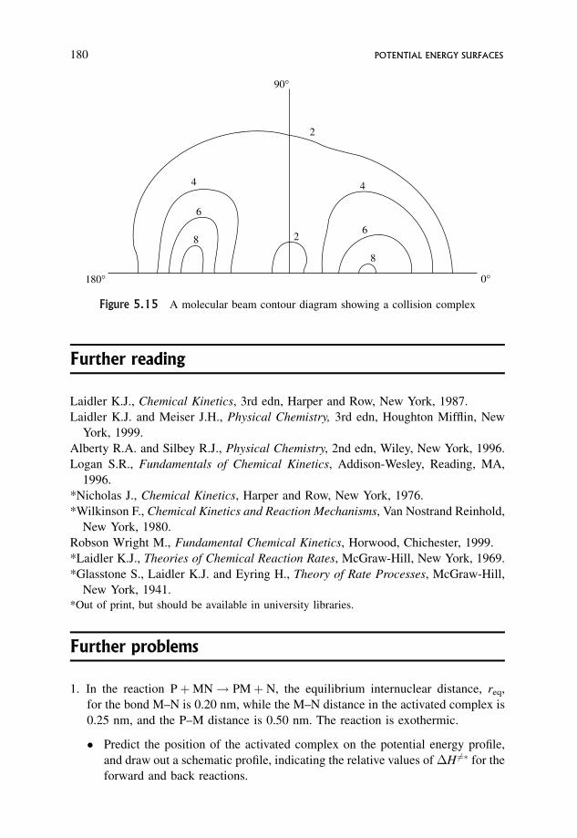
Further reading
Laidler K.J., Chemical Kinetics, 3rd edn, Harper and Row, New York, 1987.
Laidler K.J. and Meiser J.H., Physical Chemistry, 3rd edn, Houghton Mifflin, New
York, 1999.
Alberty R.A. and Silbey R.J., Physical Chemistry, 2nd edn, Wiley, New York, 1996.
Logan S.R., Fundamentals of Chemical Kinetics, Addison-Wesley, Reading, MA,
1996.
*Nicholas J., Chemical Kinetics, Harper and Row, New York, 1976.
*Wilkinson F., Chemical Kinetics and Reaction Mechanisms, Van Nostrand Reinhold,
New York, 1980.
Robson Wright M., Fundamental Chemical Kinetics, Horwood, Chichester, 1999.
*Laidler K.J., Theories of Chemical Reaction Rates, McGraw-Hill, New York, 1969.
*Glasstone S., Laidler K.J. and Eyring H., Theory of Rate Processes, McGraw-Hill,
New York, 1941.*Out of print, but should be available in university libraries.
Further problems
1. In the reaction PþMN! PMþ N, the equilibrium internuclear distance, req,
for the bond M–N is 0.20 nm, while the M–N distance in the activated complex is
0.25 nm, and the P–M distance is 0.50 nm. The reaction is exothermic.
� Predict the position of the activated complex on the potential energy profile,
and draw out a schematic profile, indicating the relative values of �H 6¼ for the
forward and back reactions.
180° 0°
90°
2
4
6
8 26
8
4
Figure 5.15 A molecular beam contour diagram showing a collision complex
180 POTENTIAL ENERGY SURFACES
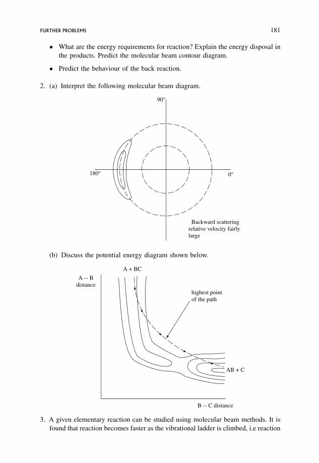
� What are the energy requirements for reaction? Explain the energy disposal in
the products. Predict the molecular beam contour diagram.
� Predict the behaviour of the back reaction.
2. (a) Interpret the following molecular beam diagram.
0°180°
90°
Backward scatteringrelative velocity fairlylarge
(b) Discuss the potential energy diagram shown below.
A + BC
A -- Bdistance
B -- C distance
AB + C
highest pointof the path
3. A given elementary reaction can be studied using molecular beam methods. It is
found that reaction becomes faster as the vibrational ladder is climbed, i.e reaction
FURTHER PROBLEMS 181
from v¼ 1 is slower than reaction from v¼ 2, which, in turn, is slower than that
from v¼ 3. What can be said about the reaction?
4. The following reactions were studied using molecular beams. Suggest interpreta-
tions of these facts, and explain the reasoning.
(a) In the reaction
Caþ NO2 ! CaOþ NO
the cross section is large and there is predominantly forward scattering.
(b) In the reaction
CH�3 þ Br2 ! CH3Brþ Br�
the cross section is small and backward scattering is observed.
(c) In the reaction
Cl� þ CH2 ¼ CHBr! CH2 ¼ CHClþ Br�
forward and backward scattering are roughly equal in amount.
(d) In the reaction of electronically excited Ca
Ca þ O2 ! CaOþ O�
the products are mainly in the ground vibrational level, v¼ 0, with only a very
low population in other higher vibrational levels.
(e) The reaction
O� þ H2 ! OH� þ H�
has a much greater cross section for H2(v¼ 1) than for H2(v¼ 0).
5. A reaction has a cross sectional area of 0.20 nm2. The radii of the two reactants are
respectively 80 and 190 pm. It is found that the translational energy of products in
the region of greatest scattering is 42.5 kJ mol1 while the product is predomi-
nantly in the ground vibrational state. The product is a diatomic molecule with
�0 ¼ 3� 1013s1. Vibrational energy¼ (vþ 1/2)h�0.
ðh ¼ 6:626� 1034J s:Þ
Deduce what you can about
(a) the physical mechanism of the reaction,
(b) the energy requirements of reaction, and energy disposal of the products,
(c) the type of scattering that would be observed and
(d) the PE contour and profile diagrams.
182 POTENTIAL ENERGY SURFACES
6 Complex Reactions in
the Gas Phase
Aims
This chapter discusses complex reactions and focuses on the chemical mechanism. Bythe end of this chapter you should be able to
� recognize and classify the large variety of complex reactions
� distinguish between chain and non-chain mechanisms
� deduce mechanisms from experimental observations
� apply the steady state treatment
� recognize that there can be kinetically equivalent mechanisms
� recognize the distinctions between steady state and pre-equilibrium treatments
� quote the characteristics of chain reactions and their kinetic features
� appreciate the significance of third bodies in complex mechanisms.
� understand the special features of surface termination
� be aware of the features of branched chain reactions and the relation betweenbranched chains and explosions, and
� be aware of the features of degenerate branching and the relation betweendegenerate branching and mild explosions
An Introduction to Chemical Kinetics. Margaret Robson Wright# 2004 John Wiley & Sons, Ltd. ISBNs: 0-470-09058-8 (hbk) 0-470-09059-6 (pbk)
6.1 Elementary and Complex Reactions
Elementary reactions occur via a single chemical step. If reaction occurs mechan-
istically as
Aþ B! products
with
mechanistic rate ¼ k½A�½B� ð6:1Þ
then the reaction is bimolecular and second order.
There are only a few elementary bimolecular reactions in the gas phase, e.g. the
reactionNOþ O3 ! NO2 þ O2
is believed to occur in one step involving the simultaneous coming together of NO
and O3 to form an activated complex, which changes configuration to give NO2 and
O2 withrate ¼ k½NO�½O3� ð6:2Þ
Many of the bimolecular reactions for which extensive data are available occur as
individual steps in reactions involving radicals, e.g.
CH�3 þ C2H6 ! CH4 þ C2H�5C2H�5 þ C2H�5 ! C4H10
Reactions between light molecules have been extensively studied in the last two
decades, generally by molecular beam techniques (see Chapter 4, Section 4.2), and
these have allowed detailed testing of the predictions made from calculated potential
energy surfaces. There are three typical mechanisms for gas phase reactions.
The stripping reactions showing forward scattering and large cross sections are
typified by reactions such as
Na� þ Cl2 ! NaClþ Cl�
Na� þ PCl3 ! NaClþ PCl�2
The rebound mechanism showing backward scattering and small cross sections is
typified byBr� þ HCl! HBrþ Cl�
K� þ CH3I! KIþ CH�3
Reactions involving collision complexes are sometimes found. Here an inter-
mediate is produced, which lasts long enough for it to perform several rotations, and
this results in symmetrical scattering. Typical reactions are
Cs� þ SF6 ! CsFþ SF�5Cl� þ CH2CHBr! CH2CHClþ Br�
184 COMPLEX REACTIONS IN THE GAS PHASE
Ion–molecule reactions have also proved fertile ground for both theoretical studies
and experiment. Here there are mainly two typical ion–molecule mechanisms:
stripping reactions such as
Nþ2� þ H2 ! N2Hþ þ H�
Nþ2� þ CH4 ! N2Hþ þ CH�3
and collision complexes for the more complex ion–molecule reactions such as
C2Hþ4� þ C2H4 ! C3Hþ5
� þ CH�3
Reaction can also be a simple breakdown of one molecule as
A! products
with
mechanistic rate ¼ k½A� ð6:3Þ
Such reactions are typified by the unimolecular decomposition of cyclopropane to
give propene, where one molecule of reactant moves into the critical configuration
and thence to products, with
rate ¼ k½C3H6� ð6:4Þ
Like the bimolecular reactions, unimolecular reactions are often found as indivi-
dual steps in complex reactions. These include the unimolecular breakdown of
molecules into radicals often found as first initiation steps and propagation steps in
chain reactions, e.g.
C2H6 ! CH�3 þ CH�3CH3CO� ! CH�3 þ CO
Complex reactions proceed in several elementary chemical steps, and have a
variety of mechanisms. But each elementary step in every mechanism also involves a
common physical mechanism, with steps of activation and deactivation by binary
collisions followed by the reaction step (Chapter 1 and Section 4.5). This can be
important when discussing individual steps in, e.g., chain reactions, Section 6.9. This
physical mechanism is
Aþ A !k1A þ A activation by collision
A þ A!k1Aþ A deactivation by collision
A þ b A !k2products reaction step
b ¼ 0; reaction is unimolecular;
b ¼ 1; reaction is bimolecular;
b ¼ 2; reaction is termolecular:
ELEMENTARY AND COMPLEX REACTIONS 185
6.2 Intermediates in Complex Reactions
Complex reactions invariably involve intermediates which are formed in some steps,
removed in others, and have a wide range of lifetimes. Longer lifetimes can result in
build-up to significant intermediate concentrations during reaction, but these inter-
mediates must also be sufficiently reactive to allow the subsequent reactions to occur.
Intermediates can also be so short lived that they are removed almost as soon as they
are formed, resulting in very, very low steady state concentrations. The lifetimes of
intermediates and their concentrations have profound effects on the analysis of the
kinetics of the reactions in which they occur.
Reminder. When steady state conditions prevail, the intermediates are highly
reactive, and the total rate of their production is virtually balanced by their total
rate of removal by reaction. They are present in very, very small and steady
concentrations, and d½I�ss=dt ¼ 0.
Reactions involving intermediates are classified as non-chain or chain. A chain
reaction is a special type of complex reaction where the distinguishing feature is the
presence of propagation steps. Here one step removes an intermediate or chain carrier
to form a second intermediate, also a chain carrier. This second chain carrier reacts to
regenerate the first chain carrier and the characteristic cycle of a chain is set up, and
continues until all the reactant is used up (see Section 6.9).
Although complex reactions can be classified as non-chain and chain, the type of
experimental data collected and the manner in which it is analysed is common to
both. The ultimate aim is to produce a mechanism, to determine the rate expression
and to find the rate constants, activation energies and A-factors for all of the
individual steps.
The following problem illustrates the variety of types of reaction which can occur.
Worked Problem 6.1
Question. Classify the following reactions in terms of the type of mechanism, i.e.
elementary, complex etc:
(a) IClþ H2 !slow
HIþ HCl
HIþ ICl !fastHClþ I2
(b) cyclo-C4H8 ! 2 C2H4
(c) 238U! 234Thþ �234Th! 234Paþ �234Pa! 234Uþ �234U! . . .
186 COMPLEX REACTIONS IN THE GAS PHASE
(d) Oþ2 þ NO! O2 þ NOþ
(e) N2O4! 2 NO2
(f) O3 þM! O2 þ O� þ M
O2 þ O� þ M! O3 þM
O3 þ O� ! 2 O2
(g) cis-di-deuterocyclopropane! trans-di-deuterocyclopropane
cis-di-deuterocyclopropane! di-deuteropropenes
(h) C2H6 ! 2 CH�3
(i) ðCH3Þ3COOCðCH3Þ3 ! 2ðCH3Þ3CO�
ðCH3Þ3CO� ! CH3COCH3 þ CH�3CH�3 þ CH�3 ! C2H6
(j) NOþ O2!k1
NO3
NO3!k1
NOþ O2
NO3 þ NO!k22 NO2
(k) N2O5! NO2 þ NO3
NO2 þ NO3 ! NO2 þ O2 þ NO
NOþ N2O5 ! 3 NO2
(l) C2H�5 þ CH3COCH3 ! C2H6 þ�CH2COCH3
(m) Br2 þM! 2 Br� þ M
Br� þ CH4 ! CH�3 þ HBr
CH�3 þ Br2 ! CH3Brþ Br�
HBrþ CH�3 ! CH4 þ Br�
2 Br� þ M! Br2 þM
(n) Krþ þ H2 ! KrHþ þ H�
Answer.
(a) Two step consecutive.
(b) One step elementary.
(c) Many step consecutive.
(d) One step elementary.
(e) Reversible reaction.
INTERMEDIATES IN COMPLEX REACTIONS 187
(f) Three step complex with the second step being the reverse of the first.
(g) Two step parallel.
(h) Elementary step in a complex reaction.
(i) Three step complex.
(j) Three step complex with the second step being the reverse of the first.
(k) Four step complex with the second step being the reverse of the first.
(l) Elementary step in a complex reaction.
(m) Five step complex with two reversible steps, i.e. steps 1 and 5 are the reverse
of each other, likewise for steps 2 and 4. This is a chain reaction. Br� and CH�3are recycled.
(n) Elementary reaction.
6.3 Experimental Data
The following is a summary of the type of data involved in the study of complex
reactions.
� Kinetic and non-kinetic information is required.
� Detection of products and intermediates is essential, and determination of their
concentration throughout reaction allows products and intermediates to be classi-
fied as present in major, minor, trace or very trace amounts. This is relatively easy
for products. Though easily detected, the very low concentrations of highly reactive
intermediates can be difficult to determine accurately (Sections 2.1.4 and 2.1.5).
Nonetheless, it is still possible to distinguish between very low steady state
concentration intermediates and higher non-steady state concentrations. This has
important consequences when unravelling the kinetics.
� Photochemically initiated reactions and quantum yields can yield vital clues in
finding the mechanism; see Section 6.8.
� Thermochemical data, and the effect of temperature on relative yields can also help
in determining mechanism.
� Kinetic studies, often from initial rates, give orders, experimental rate expressions,
rate constants and activation parameters.
188 COMPLEX REACTIONS IN THE GAS PHASE
� The proposed mechanism must fit all the experimental facts, and the mechanistic
rate expression must fit the experimental one. If these fit, the proposed mechanism
is a possible or highly plausible one, but this does not prove the mechanism to be
the correct one. Sometimes more than one mechanism can fit, called ‘kinetically
equivalent’, and a distinction between them can only be made on non-kinetic
evidence (see Section 6.6).
� The derivation of the mechanistic rate expression is considerably simplified if the
steady state treatment can be used (Sections 3.19, 3.19.1 and 3.20). When
intermediate concentrations are not sufficiently low and constant, the steady state
approximation is no longer valid. Numerical integration by computer of the
differential equations involved in the analysis, or computer simulation, may
have to be used.
6.4 Mechanistic Analysis of Complex Non-chain Reactions
The methods and techniques described above will be illustrated by the following
worked examples.
Worked Problem 6.2
This problem illustrates how to deduce a mechanism from basically non-kinetic
data.
Question. The following results were obtained from a study of the photochemical
decomposition of propanone, CH3COCH3:
CH3COCH3 ! C2H6 þ CO
1. The quantum yield of CO is unity above 120 �C, but is less than unity below
120 �C.
2. The major products are C2H6 and CO, but CH4 is also found in substantial
amounts. CH3COCOCH3 is also formed below 120 �C.
3. The minor products are CH3COCH2CH3, CH3COCH2CH2COCH3 and CH2CO.
4. Spectroscopy, esr and mass spectrometry detect CH�3, CH3COCH�2 and
CH3CO�.
5. Addition of O2 and NO reduces yields of CH4 and C2H6 to zero.
Deduce a mechanism that fits these observations.
MECHANISTIC ANALYSIS OF COMPLEX NON-CHAIN REACTIONS 189

Answer.
1. Type of process. Detection of CH�3, CH3COCH�2 and CH3CO� demonstrates a
free radical process, while the quantum yield of the product CO indicates a non-
chain mechanism (see Section 6.8).
2. Possible primary steps. A rule of thumb suggests that C–C bonds break more
readily than C–O bonds, which in turn break more easily than C–H bonds,
suggesting two possible first steps. This rule of thumb is a summary of a vast
amount of experimental data, including kinetic studies and bond dissociation
measurements.
CH3COCH3 ! 2 CH�3 þ CO ðAÞCH3COCH3 ! CH�3 þ CH3CO� ðBÞ
CH3COCOCH3 is formed from recombination of two CH3CO� radicals, and is
only found below 120 �C, suggesting step (B) as a possible primary step for
these temperatures. This is consistent with the fact that CH3CO� is relatively
stable below 120 �C and can undergo reactions other than decomposition to CO
and CH�3, i.e. recombination can occur.
At higher temperatures butane-2,3-dione, CH3COCOCH3, is no longer
produced, and this is consistent with the known very rapid decomposition of
the radical, CH3CO�, above 120 �C,
CH3CO� ! CH�3 þ CO
which suggests that (A) is the dominant primary process above 120 �C.
These inferences are also consistent with the observed quantum yields.
(a) Above 120 �C a quantum yield of unity for CO fits
CH3COCH3 ! 2 CH�3 þ CO ðAÞ
But it also fits
CH3COCH3 ! CH�3 þ CH3CO� ðBÞ
since the very rapid decomposition of CH3CO� also results in one molecule
of CO produced per molecule of CH3COCH3 decomposed.
(b) Below 120 �C the quantum yield of CO decreases, consistent with the
emergence of the competitive reaction
CH3CO� þ CH3CO� ! CH3COCOCH3
becoming possible, which will reduce the yield of CO per given amount of
CH3COCH3 decomposing.
190 COMPLEX REACTIONS IN THE GAS PHASE
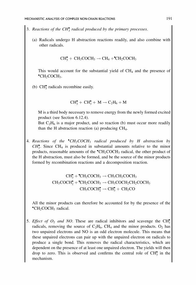
3. Reactions of the CH�3 radical produced by the primary processes.
(a) Radicals undergo H abstraction reactions readily, and also combine with
other radicals.
CH�3 þ CH3COCH3 ! CH4 þ�CH2COCH3
This would account for the substantial yield of CH4 and the presence of�CH2COCH3.
(b) CH�3 radicals recombine easily.
CH�3 þ CH�3 þ M! C2H6 þM
M is a third body necessary to remove energy from the newly formed excited
product (see Section 6.12.4).
But C2H6 is a major product, and so reaction (b) must occur more readily
than the H abstraction reaction (a) producing CH4.
4. Reactions of the �CH2COCH3 radical produced by H abstraction by
CH�3 . Since CH4 is produced in substantial amounts relative to the minor
products, reasonable amounts of the �CH2COCH3 radical, the other product of
the H abstraction, must also be formed, and be the source of the minor products
formed by recombination reactions and a decomposition reaction.
CH�3 þ�CH2COCH3 ! CH3CH2COCH3
CH3COCH�2 þ�CH2COCH3 ! CH3COCH2CH2COCH3
CH3COCH�2 ! CH�3 þ CH2CO
All the minor products can therefore be accounted for by the presence of the�CH2COCH3 radical.
5. Effect of O2 and NO. These are radical inhibitors and scavenge the CH�3radicals, removing the source of C2H6, CH4 and the minor products. O2 has
two unpaired electrons and NO is an odd electron molecule. This means that
these unpaired electrons can pair up with the unpaired electron on radicals to
produce a single bond. This removes the radical characteristics, which are
dependent on the presence of at least one unpaired electron. The yields will then
drop to zero. This is observed and confirms the central role of CH�3 in the
mechanism.
MECHANISTIC ANALYSIS OF COMPLEX NON-CHAIN REACTIONS 191
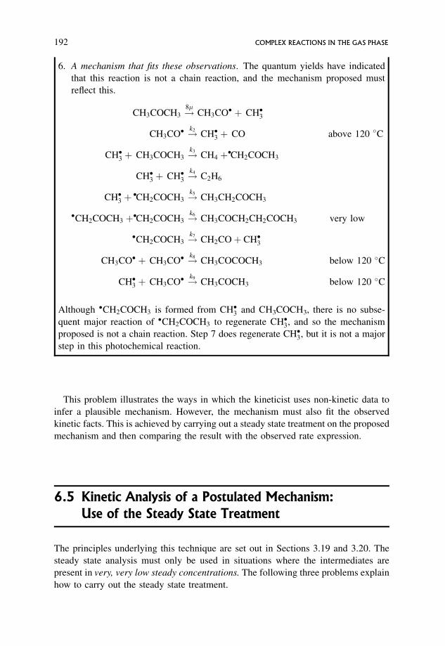
6. A mechanism that fits these observations. The quantum yields have indicated
that this reaction is not a chain reaction, and the mechanism proposed must
reflect this.
CH3COCH3 !8�
CH3CO� þ CH�3
CH3CO� !k2CH�3 þ CO above 120 �C
CH�3 þ CH3COCH3 !k3
CH4 þ�CH2COCH3
CH�3 þ CH�3 !k4
C2H6
CH�3 þ�CH2COCH3 !k5
CH3CH2COCH3
�CH2COCH3 þ�CH2COCH3 !k6
CH3COCH2CH2COCH3 very low
�CH2COCH3 !k7
CH2COþ CH�3
CH3CO� þ CH3CO� !k8CH3COCOCH3 below 120 �C
CH�3 þ CH3CO� !k9CH3COCH3 below 120 �C
Although �CH2COCH3 is formed from CH�3 and CH3COCH3, there is no subse-
quent major reaction of �CH2COCH3 to regenerate CH�3, and so the mechanism
proposed is not a chain reaction. Step 7 does regenerate CH�3, but it is not a major
step in this photochemical reaction.
This problem illustrates the ways in which the kineticist uses non-kinetic data to
infer a plausible mechanism. However, the mechanism must also fit the observed
kinetic facts. This is achieved by carrying out a steady state treatment on the proposed
mechanism and then comparing the result with the observed rate expression.
6.5 Kinetic Analysis of a Postulated Mechanism:
Use of the Steady State Treatment
The principles underlying this technique are set out in Sections 3.19 and 3.20. The
steady state analysis must only be used in situations where the intermediates are
present in very, very low steady concentrations. The following three problems explain
how to carry out the steady state treatment.
192 COMPLEX REACTIONS IN THE GAS PHASE
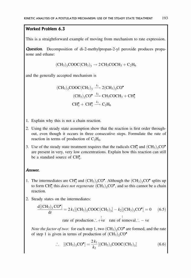
Worked Problem 6.3
This is a straightforward example of moving from mechanism to rate expression.
Question. Decomposition of di-2-methylpropan-2-yl peroxide produces propa-
none and ethane:
ðCH3Þ3COOCðCH3Þ3 ! 2 CH3COCH3 þ C2H6
and the generally accepted mechanism is
ðCH3Þ3COOCðCH3Þ3 !k1
2ðCH3Þ3CO�
ðCH3Þ3CO� !k2CH3COCH3 þ CH�3
CH�3 þ CH�3 !k3
C2H6
1. Explain why this is not a chain reaction.
2. Using the steady state assumption show that the reaction is first order through-
out, even though it occurs in three consecutive steps. Formulate the rate of
reaction in terms of production of C2H6.
3. Use of the steady state treatment requires that the radicals CH�3 and ðCH3Þ3CO�
are present in very, very low concentrations. Explain how this reaction can still
be a standard source of CH�3.
Answer.
1. The intermediates are CH�3 and ðCH3Þ3CO�. Although the ðCH3Þ3CO� splits up
to form CH�3 this does not regenerate ðCH3Þ3CO�, and so this cannot be a chain
reaction.
2. Steady states on the intermediates:
d½ðCH3Þ3 CO��dt
¼ 2 k1½ðCH3Þ3COOCðCH3Þ3� k2½ðCH3Þ3CO�� ¼ 0 ð6:5Þ
rate of production;þve"
rate of removal"
; ve
Note the factor of two: for each step 1, two ðCH3Þ3CO� are formed, and the rate
of step 1 is given in terms of production of ðCH3Þ3CO�
; ½ðCH3Þ3CO�� ¼ 2 k1
k2
½ðCH3Þ3COOCðCH3Þ3� ð6:6Þ
KINETIC ANALYSIS OF A POSTULATED MECHANISM: USE OF THE STEADY STATE TREATMENT 193
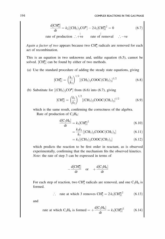
d½CH�3�dt
¼ k2½ðCH3Þ3CO�� 2 k3½CH�3�2 ¼ 0 ð6:7Þ
rate of production ;þve"
rate of removal ;ve"
Again a factor of two appears because two CH�3 radicals are removed for each
act of recombination.
This is an equation in two unknowns and, unlike equation (6.5), cannot be
solved. ½CH�3� can be found by either of two methods.
(a) Use the standard procedure of adding the steady state equations, giving
½CH�3� ¼k1
k3
� �1=2
½ðCH3Þ3COOCðCH3Þ3�1=2 ð6:8Þ
(b) Substitute for ½ðCH3Þ3CO�� from (6.6) into (6.7), giving
½CH�3� ¼k1
k3
� �1=2
½ðCH3Þ3COOCðCH3Þ3�1=2 ð6:9Þ
which is the same result, confirming the correctness of the algebra.
Rate of production of C2H6:
d½C2H6�dt
¼ k3½CH�3�2 ð6:10Þ
¼ k3k1
k3
½ðCH3Þ3COOCðCH3Þ3� ð6:11Þ
¼ k1½ðCH3Þ3COOCðCH3Þ3� ð6:12Þ
which predicts the reaction to be first order in reactant, as is observed
experimentally, confirming that the mechanism fits the observed kinetics.
Note: the rate of step 3 can be expressed in terms of
d½CH�3�dt
or þ d½C2H6�dt
For each step of reaction, two CH�3 radicals are removed, and one C2H6 is
formed.
; rate at which 3 removes CH�3 ¼ 2 k3½CH�3�2 ð6:13Þ
and
rate at which C2H6 is formed ¼ þ d½C2H6�dt
¼ k3½CH�3�2 ð6:14Þ
194 COMPLEX REACTIONS IN THE GAS PHASE
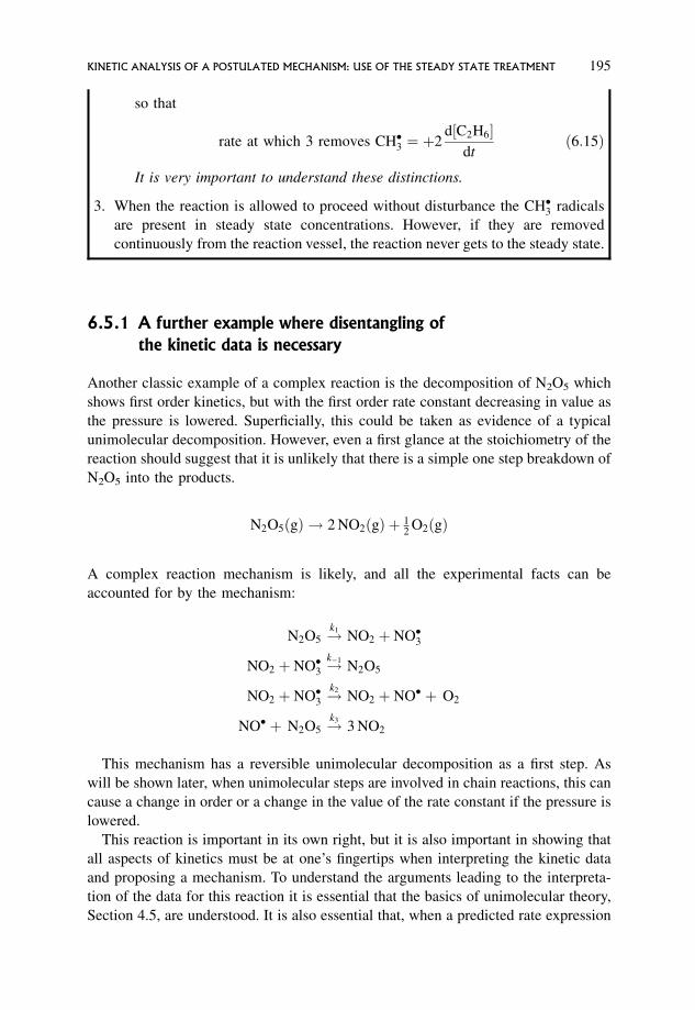
so that
rate at which 3 removes CH�3 ¼ þ2d½C2H6�
dtð6:15Þ
It is very important to understand these distinctions.
3. When the reaction is allowed to proceed without disturbance the CH�3 radicals
are present in steady state concentrations. However, if they are removed
continuously from the reaction vessel, the reaction never gets to the steady state.
6.5.1 A further example where disentangling of
the kinetic data is necessary
Another classic example of a complex reaction is the decomposition of N2O5 which
shows first order kinetics, but with the first order rate constant decreasing in value as
the pressure is lowered. Superficially, this could be taken as evidence of a typical
unimolecular decomposition. However, even a first glance at the stoichiometry of the
reaction should suggest that it is unlikely that there is a simple one step breakdown of
N2O5 into the products.
N2O5ðgÞ ! 2 NO2ðgÞ þ 12
O2ðgÞ
A complex reaction mechanism is likely, and all the experimental facts can be
accounted for by the mechanism:
N2O5 !k1
NO2 þ NO�3
NO2 þ NO�3 !k1
N2O5
NO2 þ NO�3 !k2
NO2 þ NO� þ O2
NO� þ N2O5 !k3
3 NO2
This mechanism has a reversible unimolecular decomposition as a first step. As
will be shown later, when unimolecular steps are involved in chain reactions, this can
cause a change in order or a change in the value of the rate constant if the pressure is
lowered.
This reaction is important in its own right, but it is also important in showing that
all aspects of kinetics must be at one’s fingertips when interpreting the kinetic data
and proposing a mechanism. To understand the arguments leading to the interpreta-
tion of the data for this reaction it is essential that the basics of unimolecular theory,
Section 4.5, are understood. It is also essential that, when a predicted rate expression
KINETIC ANALYSIS OF A POSTULATED MECHANISM: USE OF THE STEADY STATE TREATMENT 195
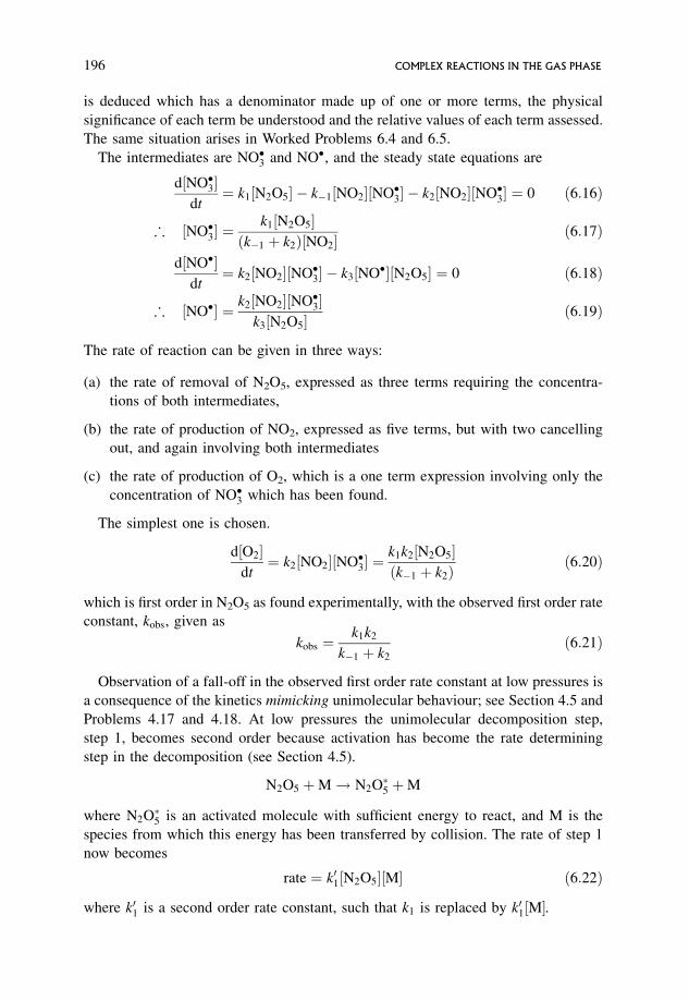
is deduced which has a denominator made up of one or more terms, the physical
significance of each term be understood and the relative values of each term assessed.
The same situation arises in Worked Problems 6.4 and 6.5.
The intermediates are NO�3 and NO�, and the steady state equations are
d½NO�3�dt
¼ k1½N2O5� k1½NO2�½NO�3� k2½NO2�½NO�3� ¼ 0 ð6:16Þ
; ½NO�3� ¼k1½N2O5�
ðk1 þ k2Þ½NO2�ð6:17Þ
d½NO��dt
¼ k2½NO2�½NO�3� k3½NO��½N2O5� ¼ 0 ð6:18Þ
; ½NO�� ¼ k2½NO2�½NO�3�k3½N2O5�
ð6:19Þ
The rate of reaction can be given in three ways:
(a) the rate of removal of N2O5, expressed as three terms requiring the concentra-
tions of both intermediates,
(b) the rate of production of NO2, expressed as five terms, but with two cancelling
out, and again involving both intermediates
(c) the rate of production of O2, which is a one term expression involving only the
concentration of NO�3 which has been found.
The simplest one is chosen.
d½O2�dt¼ k2½NO2�½NO�3� ¼
k1k2½N2O5�ðk1 þ k2Þ
ð6:20Þ
which is first order in N2O5 as found experimentally, with the observed first order rate
constant, kobs, given as
kobs ¼k1k2
k1 þ k2
ð6:21Þ
Observation of a fall-off in the observed first order rate constant at low pressures is
a consequence of the kinetics mimicking unimolecular behaviour; see Section 4.5 and
Problems 4.17 and 4.18. At low pressures the unimolecular decomposition step,
step 1, becomes second order because activation has become the rate determining
step in the decomposition (see Section 4.5).
N2O5 þM! N2O5 þM
where N2O5 is an activated molecule with sufficient energy to react, and M is the
species from which this energy has been transferred by collision. The rate of step 1
now becomes
rate ¼ k01½N2O5�½M� ð6:22Þ
where k01 is a second order rate constant, such that k1 is replaced by k01½M�.
196 COMPLEX REACTIONS IN THE GAS PHASE
If the decomposition step has moved to having activation as rate determining at low
pressures, then the reverse step of recombination must also have energy transfer as
rate determining, i.e. it must become third order at low pressures.
The rate of the reverse recombination step becomes
rate ¼ k01½NO2�½NO�3�½M� ð6:23Þ
where M is the third body required for the energy transfer step, and k01 is a third
order rate constant, such that k1 is replaced by k01½M�.Under conditions of low pressures
kobs ¼k1k2
k1 þ k3
becomes
kobs ¼k01½M�k2
k01½M� þ k2
ð6:24Þ
This, however, has no simple order, and under these conditions each of the terms in
the denominator must be examined.
The term in k01 relates to the recombination reaction converting NO2 and NO�3back to N2O5, and this reaction is in competition with the removal of NO2 and NO�3 to
produce NO2, NO� and O2. At low pressures there are fewer molecules present and
the recombination reaction requiring the simultaneous presence of three species
becomes progressively more difficult as the pressure is lowered, compared with
reaction step 2, which only requires the simultaneous presence of two molecules. This
means that
k01½NO2�½NO�3�½M� � k2½NO2�½NO�3� ð6:25Þ
; k01½M� � k2 ð6:26Þ
and so at low pressures the expression for kobs
kobs ¼k01½M�k2
k01½M� þ k2
ð6:24Þ
becomes
kobs ¼k01½M�k2
k2
¼ k01½M� ð6:27Þ
The observed rate is second order as can be shown by the following argument.
Observed rate ¼ kobs½N2O5� ð6:28Þ
KINETIC ANALYSIS OF A POSTULATED MECHANISM: USE OF THE STEADY STATE TREATMENT 197
and kobs has been shown to be equal to k01½M�, Equation (6.27)
; rate ¼ k01½M�½N2O5� ð6:29Þ
which becomes second order as observed, manifested by the calculated first order rate
constant progressively decreasing.
Remember that within any given experiment the reaction is strictly first order, see
Problems 4.17 and 4.18, but the reaction moving to second order conditions will be
shown up as the decreasing value of the first order constant.
6.6 Kinetically Equivalent Mechanisms
It is absolutely imperative to be aware that more than one mechanism may fit the
experimental observations and the observed kinetics, and that an exact fit of
prediction with experiment does not prove a given mechanism to be the correct one.
This is one of the fundamental tenets of the scientific method, viz., that it is not
possible to prove a hypothesis using experimental data, whereas it is possible to refute
a hypothesis by reference to experimental data. All that can be said is that the data fits
a given hypothesis, so that the hypothesis is a plausible one. The possibility remains
open that, in the future, experimental evidence may show that the hypothesis is not
justified.
The following problem illustrates this.
Worked Problem 6.4
Question. The reaction between nitric oxide (nitrogen monoxide) and oxygen
gives nitrogen dioxide according to the stoichiometric equation.
2 NOðgÞ þ O2ðgÞ ! 2 NO2ðgÞ
This reaction is second order in NO and first order in O2. The following
mechanisms can be proposed.
Mechanism A
2 NO !k1N2O2
N2O2 !k1
2 NO
N2O2 þ O2 !k2
2 NO2
198 COMPLEX REACTIONS IN THE GAS PHASE
Mechanism B
NOþ O2 !k1
NO3
NO3 !k1
NOþ O2
NO3 þ NO !k22 NO2
1. Assuming the steady state approximation, deduce the rate expressions for each
mechanism.
2. Under what conditions will these mechanisms fit the experimental data and be
kinetically equivalent? Hint: consider the denominator and the mathematical
and chemical significance of each term.
3. What do the above analyses imply about the likelihood of the reversible steps
being at equilibrium?
4. A further possibility is that the reaction occurs as an elementary termolecular
reaction: which mechanism(s) is the more likely?
Answer.
1. Applying the steady state treatment.
(a) Mechanism A. The intermediate is N2O2, and the rate of reaction is given in
terms of step 2:
þ d½N2O2�dt
¼ k1½NO�2 k1½N2O2� k2½N2O2�½O2� ¼ 0 ð6:30Þ
; ½N2O2� ¼k1½NO�2
k1 þ k2½O2�ð6:31Þ
þ d½NO2�dt
¼ 2 k2½N2O2�½O2� ð6:32Þ
¼ 2 k1k2½NO�2½O2�k1 þ k2½O2�
ð6:33Þ
The factor of two is included, since two molecules of NO2 are formed per
step of reaction.
(b) Mechanism B. The intermediate is now NO3, but the rate of reaction is still
given by the rate of step 2.
KINETICALLY EQUIVALENT MECHANISMS 199
þ d½NO3�dt
¼ k1½NO�½O2� k1½NO3� k2½NO3�½NO� ¼ 0 ð6:34Þ
; ½NO3� ¼k1½NO�½O2�
k1 þ k2½NO� ð6:35Þ
þ d½NO2�dt
¼ 2 k2½NO3�½NO� ð6:36Þ
¼ 2 k1k2½NO�2½O2�k1 þ k2½NO� ð6:37Þ
Note the factor of two.
These two mechanisms give the same type of algebraic expression, but the
actual expressions are different and neither fits the experimental rate
expression:
observed rate ¼ kobs½NO�2½O2� ð6:38Þ
2. However, if in mechanism A k2½O2� can be ignored with respect to k1 then
k1 � k2½O2� ð6:39Þ
and
k1½N2O2� � k2½N2O2�½O2� ð6:40Þ
which implies that
rate of reverse step� the rate of reaction step
and most of the intermediate is removed by the reverse step and very, very
little by reaction, suggesting that reaction is unlikely to disturb the equilibrium,
and
If in mechanism B k2½NO� can be ignored with respect to k1 then
k1 � k2½NO� ð6:41Þ
and
k1½NO3� � k2½NO�½NO3� ð6:42Þ
which implies that
rate of reverse step� rate of reaction step
and most of the intermediate is removed by the reverse step and very, very little
by reaction, suggesting that reaction is unlikely to disturb the equilibrium.
200 COMPLEX REACTIONS IN THE GAS PHASE
If these approximations are made, then both expressions reduce to
2k1k2½NO�2½O2�k1
ð6:43Þ
compatible with the observed rate expression above, with
kobs ¼2 k1k2
k1
ð6:44Þ
3. Hence, if these conditions hold, both mechanisms reduce to the same rate
expression and must be kinetically equivalent. Non-kinetic evidence is required
to distinguish them.
As shown, these approximations imply that for both mechanisms reaction is
unlikely to disturb the equilibrium.
This conclusion can be demonstrated by carrying out a kinetic analysis
assuming that the reversible reaction is at equilibrium throughout the reaction.
This type of analysis is valid only if there is equilibrium so far as the reversible
reaction is concerned.
Assuming mechanism A:
K ¼½N2O2�equil
½NO�2equil
ð6:45Þ
; ½N2O2�equil ¼ K½NO�2equil ð6:46Þ
þ d½NO2�dt
¼ 2 k2½N2O2�½O2� ð6:32Þ
¼ 2 k2K½NO�2½O2� ð6:47Þ
which fits the observed kinetics and the steady state analysis with the
approximation k1 � k2½O2�. A similar pre-equilibrium analysis on mechanism
B will yield the same result.
4. If the reaction were a termolecular elementary reaction
NOþ NOþ O2 ! 2 NO2
then the predicted kinetics would be
d½NO2�dt
¼ 2 k½NO�2½O2� ð6:48Þ
kinetically equivalent to the previous two complex mechanisms.
Either of the two complex mechanisms would be more likely than the termo-
lecular reaction, since the former only require two molecules to come together
simultaneously in any given step. The termolecular mechanism would require the
much more unlikely situation of a three body collision.
KINETICALLY EQUIVALENT MECHANISMS 201
6.7 A Comparison of Steady State Procedures and
Equilibrium Conditions in the Reversible Reaction
Many complex reactions involve a reversible step followed by one or more other steps. If the
intermediate(s) are present in steady state concentrations, then the steady state analysis will
give a general procedure for deducing the rate expression. If the intermediate(s) are present
in equilibrium concentrations, an equilibrium analysis is appropriate. But if the inter-
mediate(s) are not in either of these two categories, analysis becomes very complex
(Sections 3.22 and 8.4). A comparison of the predicted and observed rate expressions can
give considerable insight, e.g. Problem 6.4 above, and Problem 6.5 below.
Worked Problem 6.5
This problem focuses on the difference between steady state methods and the
assumption of a pre-equilibrium for a reaction where the first two steps are reversible.
Question. The following mechanism is common to both inorganic and organic
reactions:
RX !k1Rþ þ X
Rþ þ X !k1RX
Rþ þ Y !k2RY
� Carry out a steady state treatment, and find the conditions under which this
reaction would be
(a) first order in both RX and Y but inverse first order in X,
(b) simple first order in RX.
� Now assume that the reversible reaction is at equilibrium, and deduce the rate
expression.
� By comparing these two treatments, find the conditions under which the
pre-equilibrium would be set up.
Answer.
� The steady state treatment
d½Rþ�dt¼ k1½RX� k1½Rþ�½X� k2½Rþ�½Y� ¼ 0 ð6:49Þ
½Rþ� ¼ k1½RX�k1½X� þ k2½Y�
ð6:50Þ
þ d½RY�dt¼ k2½Rþ�½Y� ð6:51Þ
¼ k1k2½RX�½Y�k1½X� þ k2½Y�
ð6:52Þ
202 COMPLEX REACTIONS IN THE GAS PHASE
Under steady state conditions, the reaction has complex kinetics with no simple
order. As in the previous problem, there is a denominator made up of two terms,
and again both terms should be considered in relation to each other. Doing so,
(a) Ifk1½X� � k2½Y� ð6:53Þ
then
k1½Rþ�½X� � k2½Rþ�½Y� ð6:54Þwhich implies that
rate of reverse step� rate of reaction step
and most of the intermediate is removed by the reverse step rather than by
reaction.
The rate expression, Equation (6.52), then reduces to
d½RY�dt¼ k1k2½RX�½Y�
k1½X�ð6:55Þ
with reaction first order in RX and Y and inverse first order in X.
(b) Ifk1½X� � k2½Y� ð6:56Þ
then
k1½Rþ�½X� � k2½Rþ�½Y� ð6:57Þwhich implies that
rate of reverse step� rate of reaction step:
Most of the intermediate is removed by reaction.
The rate expression, equation (6.52) then reduces to
d½RY�dt¼ k1½RX� ð6:58Þ
with reaction simple first order in reactant.
� If the reversible reaction is at equilibrium throughout reaction, then
K ¼ ½Rþ�½X�½RX�
� �equil
ð6:59Þ
; ½Rþ�equil ¼K½RX�equil
½X�equil
ð6:60Þ
d½RY�dt¼ k2½Rþ�equil½Y� ð6:61Þ
¼k2K½RX�equil½Y�½X�equil
ð6:62Þ
¼k2k1½RX�equil½Y�
k1½X�equil
ð6:63Þ
COMPARISON OF STEADY STATE PROCEDURES AND EQUILIBRIUM CONDITIONS 203
This corresponds to the steady state analysis (a), where most of the intermediate
is removed by the reverse reaction and very little by reaction. It is only under
these conditions that the pre-equilibrium is likely to be set up and maintained
throughout reaction; see Section 8.4.
Note. It is very instructive to compare this analysis with that for the reaction of NO
with O2. Although these two reactions are totally different chemically, they analyse
kinetically to be of the same algebraic form with the same chemical implications.
This is a very common situation in kinetics, and there are many other rate processes
which exhibit this algebraic form with a denominator. Other algebraic forms likewise
can result on analysis for widely disparate reactions.
6.8 The Use of Photochemistry in Disentangling
Complex Mechanisms
If a reaction can be initiated photochemically, a further route to investigating the
mechanism and evaluating the rate constants becomes possible.
Radiation can be used to initiate a reaction (see Section 2.2.4). When molecules
absorb radiation they are excited and often split up into radicals. Normally one
molecule absorbs one quantum of radiation. This enables the rate of formation of the
radicals produced as a result of absorption to be found from a measure of the radiation
absorbed. These radicals may then react in a sequence of reactions, whereby more
reactant is removed independently of the initial breakdown under the influence of
radiation. The quantum yield is defined as the number of reactant molecules
transformed per quantum absorbed, and gives a measure of how many molecules
of reactant eventually react as a result of the initial first breakdown. If the quantum
yield is large, this is conclusive evidence of a chain reaction, where many reactant
molecules decompose per quantum absorbed.
The identity of the radicals formed from the initially excited molecule can be
studied spectroscopically. If conventional radiation sources are used, the radicals will
be formed in steady state concentrations and their rates of formation and removal
cannot be measured. If, however, flash or laser photolysis is used the radicals are
formed in much larger concentrations and their concentration–time profiles can be
determined spectroscopically; see Sections 2.1.4 and 2.5.2. From this, rate constants
for the overall formation and removal of these radicals can be found.
6.8.1 Kinetic features of photochemistry
� The term ‘primary process’ describes both the production of the excited species and
its subsequent decomposition into atoms and free radicals. ‘Secondary processes’
204 COMPLEX REACTIONS IN THE GAS PHASE
describe all subsequent reactions of the radicals. The overall reaction can be chain
or non-chain.
� The ‘law of photochemical equivalence’ states that one molecule absorbs one
quantum, which allows a calculation of the rate of formation of radicals from the
intensity of the radiation absorbed. This can be extremely useful in the kinetic
analysis as it gives a rate constant for the first step in the sequence. For example
CH3COCH3 þ h� ! CH3COCH3 ! 2 CH�3 þ CO
produces excited CH3COCH3 molecules as the primary process, and the rate of
absorption of photons will give
rate of formation of CO ¼ Iabs ð6:64Þ
rate of formation of CH�3 ¼ 2 Iabs ð6:65Þ
rate of removal of CH3COCH3 ¼ Iabs ð6:66Þ
� The quantum yield is given by the number of reactant molecules transformed per
quantum absorbed. The quantum yield of the primary process is unity, unless any
collision processes, emission or fluorescence compete.
If the photochemical reaction were a single elementary step, then the quantum
yield in terms of the reactants would also be unity. However, the quantum yield may
differ from unity for several reasons.
(a) The quantum yield is a small integral number for complex, but non-chain
reactions where more than one reactant molecule reacts per quantum absorbed
HBrþ h� ! H� þ Br�
HBrþ H� ! H2 þ Br�
Br� þ Br� þ M! Br2 þM
where M is a third body which removes excess energy from the newly formed Br2
molecule; see Section 6.12.4.
In the primary process one quantum is absorbed by one molecule of HBr, as a result
of which a second molecule of HBr can react. For one quantum absorbed, effectively
two molecules of HBr react, giving a quantum yield of two for the reactant.
(b) The quantum yield can be less than unity if
(i) the radicals or intermediates formed in the primary process can recombine,
so that the net removal of reactant will be less than the removal of reactant in
the primary step, or
(ii) the excited molecule can be deactivated before it can react.
(c) The quantum yield can be large, and often very large, and this is specific to, and
diagnostic of, chain reactions. For every act of initiation, the primary process, the
THE USE OF PHOTOCHEMISTRY IN DISENTANGLING COMPLEX MECHANISMS 205
propagation steps ensure that large numbers of reactants can react. The mechan-
ism for the reaction of CO and Cl2 to give COCl2 is
Cl2 þ h� ! 2 Cl�
Cl� þ CO! COCl�
COCl� þ Cl2 ! COCl2 þ Cl�
COCl� þ Cl� ! inert species
The Cl� produced in the primary process is involved in the propagation steps
which result in many molecules of Cl2 and CO being transformed, giving a very
large quantum yield.
The quantum yield is found by measuring the amount of reactant removed, or
product formed, as a result of absorption of a given amount of radiation. The
stoichiometry of the reactions involved may be such that the quantum yields for
reactants and products differ. For instance, in the decomposition of HBr quoted the
quantum yield in terms of HBr is two, and in terms of H2 and Br2 is unity.
6.8.2 The reaction of H2 with I2
For many years this reaction was quoted as the classic example of an elementary
bimolecular reaction, and used as a test of collision and transition state theories, but it
has now been shown to be a complex non-chain reaction.
Photochemical experiments show iodine atoms to be involved, and molecular
beams subsequently confirmed this by shooting beams of H2 and I2 molecules at each
other and finding no reaction. In contrast, beams of H2 molecules and I� atoms
resulted in reaction.
When H2 and I2 react thermally
observed rate ¼ kthermalobs ½H2�½I2� ð6:67Þ
There are two mechanisms which can account for this:
(a) direct molecular combination: H2 þ I2!kmolec 2 HI
(b) an atomic mechanism: I2 þM! 2 I� þ M
H2 þ I� þ I�!katomic2 HI
These two schemes are kinetically equivalent, as will be shown below.
If both mechanisms contribute to the thermal rate
rate ¼ kmolec½H2�½I2� þ katomic½H2�½I��2 ð6:68Þ¼ kthermal
obs ½H2�½I2� ð6:69Þ
206 COMPLEX REACTIONS IN THE GAS PHASE
Two situations can arise:
(a) the iodine atoms are in equilibrium with molecular iodine,
(b) equilibrium is not set up, and only a stationary state concentration of iodine
atoms is present.
Equilibrium is set up between I� and molecular I2
I2! 2 I�
where
K ¼ ½I��2
½I2�
!equil
ð6:70Þ
and
½I��2eq ¼ K½I2�equil ð6:71Þ
Substitution into Equation (6.68) gives
rate ¼ ðkmolec þ katomicKÞ½H2�equil½I2�equil ð6:72Þ
and this must be equal to the thermal rate, giving for the equilibrium situation
kthermalobs ¼ kmolec þ katomicK ð6:73Þ
¼ a constant ð6:74Þ
No matter whether reaction goes totally by the molecular mechanism, katomic ¼ 0, or
totally by the atomic mechanism, kmolec ¼ 0, or by both mechanisms simultaneously,
the rate law is predicted to be strictly second order and there is no kinetic means of
determining which mechanism holds. The two schemes are kinetically equivalent.
A stationary state only is set up
Equilibrium is not set up and Equation (6.70) does not hold. However, the rate law
still holds and Equation (6.68) can be transformed into
rate ¼ kmolec½H2�½I2� þkatomic½H2�½I2�½I��2steady state
½I2�ð6:75Þ
¼ kmolec þ katomic
½I��2steady state
½I2�
( )½H2�½I2� ð6:76Þ
THE USE OF PHOTOCHEMISTRY IN DISENTANGLING COMPLEX MECHANISMS 207

now giving
kthermalobs ¼ kmolec þ katomic
½I��2steady state
½I2�
( )ð6:77Þ
¼ a constant ð6:78Þ
provided that a steady state is maintained throughout the experiment. If Equa-
tion (6.77) holds then kthermalobs takes a numerical value which depends on the particular
steady state concentration set up during the experiment. If it were possible to set up a
series of different steady state concentrations and measure kthermalobs for each, then the
value would depend on the steady state concentration.
There is no way that the steady state concentration can be varied if the thermal
reaction is studied at constant temperature. However, if the reaction is studied
photochemically with a series of differing intensities of radiation, then a series of
different steady state concentrations can be set up. The kobs value for the photo-
chemical reaction would then depend on the intensity. Equation (6.77) is then
transformed into
kphotochemicalobs ¼ kmolec þ katomic
½I��2steady state
½I2�
( )ð6:79Þ
¼ a constant ð6:80Þ
where the constant now depends on the intensity of the radiation used. The constant
would only be independent of the intensity if katomic were zero.
Such experiments have been carried out, and the photochemical kphotochemicalobs has
been shown to vary with intensity in such a manner that the equation
kphotochemicalobs ¼ kmolec þ katomic
½I��2steady state
½I2�
!ð6:79Þ
fits the data only if kmolec equals zero, showing that only the atomic mechanism is
operative under photochemical conditions.
Extension of the rate constant data to the thermal reaction shows that this too can
be accounted for totally by the atomic mechanism.
6.9 Chain Reactions
A chain reaction involves at least two highly reactive intermediates, called chain
carriers, which take part in a cycle of reactions called propagation. In the first
propagation step one intermediate is removed and the second formed. This inter-
mediate then goes on to regenerate the first intermediate in the second propagation
step. At least one step removes reactant, and at least one forms product. The cycle
208 COMPLEX REACTIONS IN THE GAS PHASE
continues until either the reactant is all used up, or one, or both, of the chain carriers
are removed by conversion into an unreactive species in the chain-breaking steps of
termination. Most of the reaction, therefore, occurs in propagation, which is thus the
source of the major products and the means whereby most of the reactant is removed.
Termination steps are generally recombination reactions, though disproportionation
can occur. Recombination reactions occur when two radicals combine to give one
molecule, while disproportionation occurs when two radicals react to form two
molecules, rather than recombining to form one:
C2H�5 þ C2H�5 ! C4H10 recombination
C2H�5 þ C2H�5 ! C2H4 þ C2H6 disproportionation
Both are termination reactions, and the net effect is removal of chain carriers.
Identification of the minor products will give evidence as to the relative proportions
of each. Their essential feature is removal of chain carriers to form inert species
incapable of carrying on the chain. They occur infrequently compared with propaga-
tion, and so produce the minor products.
The initiation step(s) first produces a chain carrier enabling propagation to be set
up. Since one step of initiation can set up a long cycle of propagation events, very
little reactant is used up in initiation.
Other types of step can occur, such as inhibition, but these are not essential for the
characterization of a reaction as a chain. Inhibition occurs when a chain carrier reacts
with a product in the reverse of a propagation step, or with an added substance, and as
a consequence the overall rate is reduced.
6.9.1 Characteristic experimental features of chain reactions
� Chains always involve highly reactive atoms or radicals, often present in very low
steady state concentrations.
� The rate of reaction can be of simple order, either first, second or non-integral, but
it can also be complex. A complex order always means a complex mechanism, but
a simple order need not mean a simple mechanism.
� The shape of the rate–time plot is significant: a maximum in rate suggests a chain
reaction. Build-up to a maximum corresponds to build-up to the steady state, after
which the concentration of chain carriers remains constant and the overall rate,
a composite quantity, gradually decreases as in a typical non-chain reaction. When
there is a complex mechanism the overall rate constant is also composite and is
made up of one or more rate constants relating to individual steps in the
mechanism; e.g. in Chapter 3, Problem 3.18, the mechanism for the decomposition
of C3H8 is a chain mechanism and the analysis gave
rate of reaction ¼ k2ðk1=2 k4Þ1=2½C3H8�3=2 ð6:81Þ
CHAIN REACTIONS 209
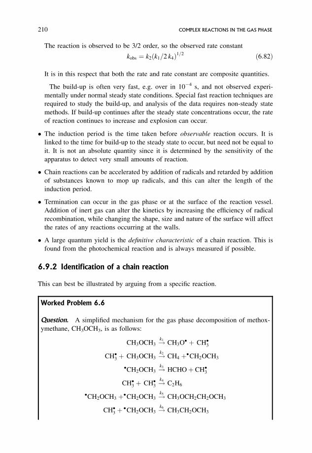
The reaction is observed to be 3/2 order, so the observed rate constant
kobs ¼ k2ðk1=2 k4Þ1=2 ð6:82Þ
It is in this respect that both the rate and rate constant are composite quantities.
The build-up is often very fast, e.g. over in 104 s, and not observed experi-
mentally under normal steady state conditions. Special fast reaction techniques are
required to study the build-up, and analysis of the data requires non-steady state
methods. If build-up continues after the steady state concentrations occur, the rate
of reaction continues to increase and explosion can occur.
� The induction period is the time taken before observable reaction occurs. It is
linked to the time for build-up to the steady state to occur, but need not be equal to
it. It is not an absolute quantity since it is determined by the sensitivity of the
apparatus to detect very small amounts of reaction.
� Chain reactions can be accelerated by addition of radicals and retarded by addition
of substances known to mop up radicals, and this can alter the length of the
induction period.
� Termination can occur in the gas phase or at the surface of the reaction vessel.
Addition of inert gas can alter the kinetics by increasing the efficiency of radical
recombination, while changing the shape, size and nature of the surface will affect
the rates of any reactions occurring at the walls.
� A large quantum yield is the definitive characteristic of a chain reaction. This is
found from the photochemical reaction and is always measured if possible.
6.9.2 Identification of a chain reaction
This can best be illustrated by arguing from a specific reaction.
Worked Problem 6.6
Question. A simplified mechanism for the gas phase decomposition of methox-
ymethane, CH3OCH3, is as follows:
CH3OCH3 !k1
CH3O� þ CH�3
CH�3 þ CH3OCH3 !k2
CH4 þ�CH2OCH3
�CH2OCH3 !k3
HCHOþ CH�3
CH�3 þ CH�3 !k4
C2H6
�CH2OCH3 þ�CH2OCH3 !k5
CH3OCH2CH2OCH3
CH�3 þ�CH2OCH3 !k6
CH3CH2OCH3
210 COMPLEX REACTIONS IN THE GAS PHASE
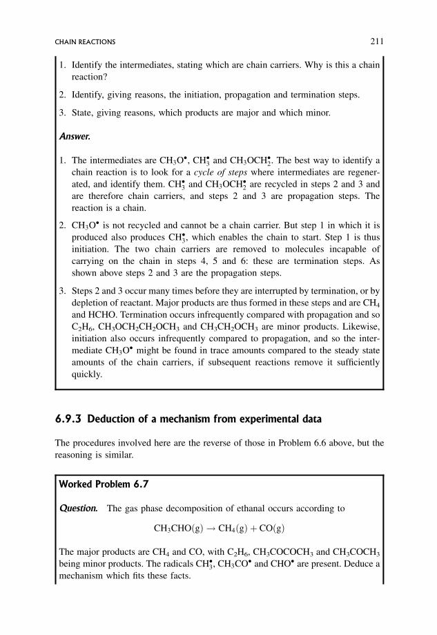
1. Identify the intermediates, stating which are chain carriers. Why is this a chain
reaction?
2. Identify, giving reasons, the initiation, propagation and termination steps.
3. State, giving reasons, which products are major and which minor.
Answer.
1. The intermediates are CH3O�, CH�3 and CH3OCH�2. The best way to identify a
chain reaction is to look for a cycle of steps where intermediates are regener-
ated, and identify them. CH�3 and CH3OCH�2 are recycled in steps 2 and 3 and
are therefore chain carriers, and steps 2 and 3 are propagation steps. The
reaction is a chain.
2. CH3O� is not recycled and cannot be a chain carrier. But step 1 in which it is
produced also produces CH�3, which enables the chain to start. Step 1 is thus
initiation. The two chain carriers are removed to molecules incapable of
carrying on the chain in steps 4, 5 and 6: these are termination steps. As
shown above steps 2 and 3 are the propagation steps.
3. Steps 2 and 3 occur many times before they are interrupted by termination, or by
depletion of reactant. Major products are thus formed in these steps and are CH4
and HCHO. Termination occurs infrequently compared with propagation and so
C2H6, CH3OCH2CH2OCH3 and CH3CH2OCH3 are minor products. Likewise,
initiation also occurs infrequently compared to propagation, and so the inter-
mediate CH3O� might be found in trace amounts compared to the steady state
amounts of the chain carriers, if subsequent reactions remove it sufficiently
quickly.
6.9.3 Deduction of a mechanism from experimental data
The procedures involved here are the reverse of those in Problem 6.6 above, but the
reasoning is similar.
Worked Problem 6.7
Question. The gas phase decomposition of ethanal occurs according to
CH3CHOðgÞ ! CH4ðgÞ þ COðgÞ
The major products are CH4 and CO, with C2H6, CH3COCOCH3 and CH3COCH3
being minor products. The radicals CH�3, CH3CO� and CHO� are present. Deduce a
mechanism which fits these facts.
CHAIN REACTIONS 211
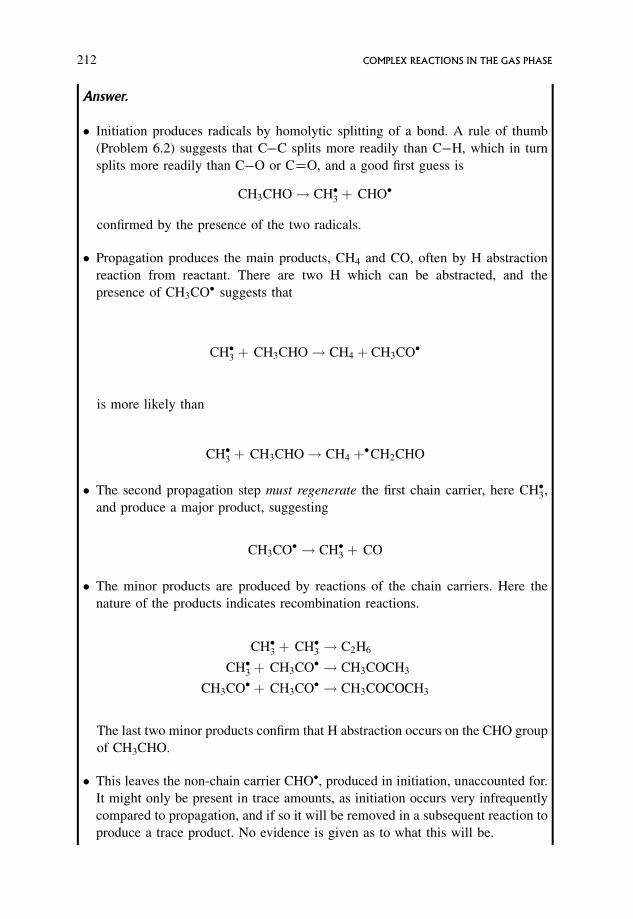
Answer.
� Initiation produces radicals by homolytic splitting of a bond. A rule of thumb
(Problem 6.2) suggests that CC splits more readily than CH, which in turn
splits more readily than CO or CO, and a good first guess is
CH3CHO! CH�3 þ CHO�
confirmed by the presence of the two radicals.
� Propagation produces the main products, CH4 and CO, often by H abstraction
reaction from reactant. There are two H which can be abstracted, and the
presence of CH3CO� suggests that
CH�3 þ CH3CHO! CH4 þ CH3CO�
is more likely than
CH�3 þ CH3CHO! CH4 þ�CH2CHO
� The second propagation step must regenerate the first chain carrier, here CH�3,
and produce a major product, suggesting
CH3CO� ! CH�3 þ CO
� The minor products are produced by reactions of the chain carriers. Here the
nature of the products indicates recombination reactions.
CH�3 þ CH�3 ! C2H6
CH�3 þ CH3CO� ! CH3COCH3
CH3CO� þ CH3CO� ! CH3COCOCH3
The last two minor products confirm that H abstraction occurs on the CHO group
of CH3CHO.
� This leaves the non-chain carrier CHO�, produced in initiation, unaccounted for.
It might only be present in trace amounts, as initiation occurs very infrequently
compared to propagation, and if so it will be removed in a subsequent reaction to
produce a trace product. No evidence is given as to what this will be.
212 COMPLEX REACTIONS IN THE GAS PHASE
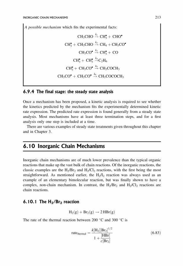
A possible mechanism which fits the experimental facts:
CH3CHO !k1CH�3 þ CHO�
CH�3 þ CH3CHO !k2CH4 þ CH3CO�
CH3CO� !k3CH�3 þ CO
CH�3 þ CH�3 !k4
C2H6
CH�3 þ CH3CO� !k5CH3COCH3
CH3CO� þ CH3CO� !k6CH3COCOCH3
6.9.4 The final stage: the steady state analysis
Once a mechanism has been proposed, a kinetic analysis is required to see whether
the kinetics predicted by the mechanism fits the experimentally determined kinetic
rate expression. The predicted rate expression is found generally from a steady state
analysis. Most mechanisms have at least three termination steps, and for a first
analysis only one step is included at a time.
There are various examples of steady state treatments given throughout this chapter
and in Chapter 3.
6.10 Inorganic Chain Mechanisms
Inorganic chain mechanisms are of much lower prevalence than the typical organic
reactions that make up the vast bulk of chain reactions. Of the inorganic reactions, the
classic examples are the H2/Br2 and H2/Cl2 reactions, with the first being the most
straightforward. As mentioned earlier, the H2/I2 reaction was always used as an
example of an elementary bimolecular reaction, but was finally shown to have a
complex, non-chain mechanism. In contrast, the H2/Br2 and H2/Cl2 reactions are
chain reactions.
6.10.1 The H2/Br2 reaction
H2ðgÞ þ Br2ðgÞ ! 2 HBrðgÞ
The rate of the thermal reaction between 200 �C and 300 �C is
ratethermal ¼k½H2�½Br2�1=2
1þ ½HBr�c½Br2�
ð6:83Þ
INORGANIC CHAIN MECHANISMS 213
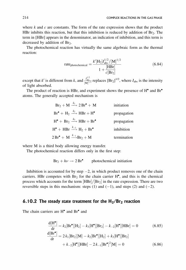
where k and c are constants. The form of the rate expression shows that the product
HBr inhibits this reaction, but that this inhibition is reduced by addition of Br2. The
term in [HBr] appears in the denominator, an indication of inhibition, and this term is
decreased by addition of Br2.
The photochemical reaction has virtually the same algebraic form as the thermal
reaction:
ratephotochemical ¼k0½H2�I1=2
abs =½M�1=2
1þ ½HBr�c½Br2�
ð6:84Þ
except that k0 is different from k, andI
1=2
abs
½M�1=2 replaces [Br2]1/2, where Iabs is the intensity
of light absorbed.
The product of reaction is HBr, and experiment shows the presence of H� and Br�
atoms. The generally accepted mechanism is
Br2 þM !k12 Br� þ M initiation
Br� þ H2 !k2
HBrþ H� propagation
H� þ Br2 !k3
HBrþ Br� propagation
H� þ HBr !k2H2 þ Br� inhibition
2 Br� þ M !k1Br2 þM termination
where M is a third body allowing energy transfer.
The photochemical reaction differs only in the first step:
Br2 þ h� ! 2 Br� photochemical initiation
Inhibition is accounted for by step 2, in which product removes one of the chain
carriers. HBr competes with Br2 for the chain carrier H�, and this is the chemical
process which accounts for the term ½HBr�=½Br2� in the rate expression. There are two
reversible steps in this mechanism: steps (1) and (1), and steps (2) and (2).
6.10.2 The steady state treatment for the H2/Br2 reaction
The chain carriers are H� and Br� and
d½H��dt¼ k2½Br��½H2� k3½H��½Br2� k2½H��½HBr� ¼ 0 ð6:85Þ
d½Br��dt¼ 2 k1½Br2�½M� k2½Br��½H2� þ k3½H��½Br2�
þ k2½H��½HBr� 2 k1½Br��2½M� ¼ 0 ð6:86Þ
214 COMPLEX REACTIONS IN THE GAS PHASE
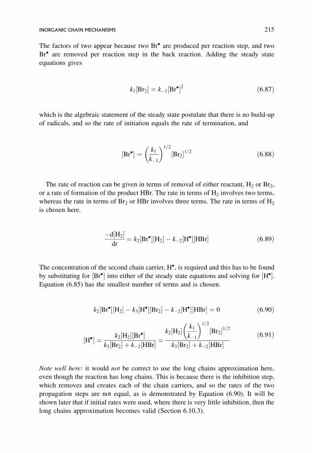
The factors of two appear because two Br� are produced per reaction step, and two
Br� are removed per reaction step in the back reaction. Adding the steady state
equations gives
k1½Br2� ¼ k1½Br��2 ð6:87Þ
which is the algebraic statement of the steady state postulate that there is no build-up
of radicals, and so the rate of initiation equals the rate of termination, and
½Br�� ¼ k1
k1
� �1=2
½Br2�1=2 ð6:88Þ
The rate of reaction can be given in terms of removal of either reactant, H2 or Br2,
or a rate of formation of the product HBr. The rate in terms of H2 involves two terms,
whereas the rate in terms of Br2 or HBr involves three terms. The rate in terms of H2
is chosen here.
d½H2�dt
¼ k2½Br��½H2� k2½H��½HBr� ð6:89Þ
The concentration of the second chain carrier, H�, is required and this has to be found
by substituting for ½Br�� into either of the steady state equations and solving for ½H��.Equation (6.85) has the smallest number of terms and is chosen.
k2½Br��½H2� k3½H��½Br2� k2½H��½HBr� ¼ 0 ð6:90Þ
½H�� ¼ k2½H2�½Br��k3½Br2� þ k2½HBr� ¼
k2½H2�k1
k1
� �1=2
½Br2�1=2
k3½Br2� þ k2½HBr�ð6:91Þ
Note well here: it would not be correct to use the long chains approximation here,
even though the reaction has long chains. This is because there is the inhibition step,
which removes and creates each of the chain carriers, and so the rates of the two
propagation steps are not equal, as is demonstrated by Equation (6.90). It will be
shown later that if initial rates were used, where there is very little inhibition, then the
long chains approximation becomes valid (Section 6.10.3).
INORGANIC CHAIN MECHANISMS 215
Substituting into Equation (6.89) gives
d½H2�dt
¼ k2
k1
k1
� �1=2
½Br2�1=2½H2� k2½HBr�k2½H2�
k1
k1
� �1=2
½Br2�1=2
k3½Br2� þ k2½HBr�
8>>><>>>:
9>>>=>>>;
ð6:92Þ
¼ k2
k1
k1
� �1=2
½Br2�1=2½H2� 1 k2½HBr�k3½Br2� þ k2½HBr�
� �ð6:93Þ
¼ k2
k1
k1
� �1=2
½Br2�1=2½H2�k3½Br2�
k3½Br2� þ k2½HBr�
� �ð6:94Þ
¼ k2
k1
k1
� �1=2
½Br2�1=2½H2� 1þ k2½HBr�k3½Br2�
� �1
ð6:95Þ
¼k2
k1
k1
� �1=2
½Br2�1=2½H2�
1þ k2½HBr�k3½Br2�
ð6:96Þ
which, when compared with Equation (6.83) for the thermal rate, gives
k ¼ k2
k1
k1
� �1=2
and c ¼ k3
k2
ð6:97Þ and ð6:98Þ
A similar analysis for the photochemical rate replaces the rate of thermal initiation,
2 k1½Br2�½M�, by the rate of photochemical initiation 2 Iabs, giving
photochemical rate ¼ d½H2�dt¼
k2
1
k1½M�
� �1=2
I1=2abs ½H2�
1þ k2½HBr�k3½Br2�
ð6:99Þ
6.10.3 Reaction without inhibition
Inhibition can be reduced to virtually zero if initial rates are used. Very little product,
HBr, will have built up during the period of experimental measurements and the rate
of the inhibition step will be virtually zero. In the steady state expression for ½H��,Equation (6.85), the term in k2 will drop out, leaving
d½H��dt¼ k2½Br��½H2� k3½H��½Br2� ¼ 0 ð6:100Þ
216 COMPLEX REACTIONS IN THE GAS PHASE
and
k2½Br��½H2� ¼ k3½H��½Br2� ð6:101Þ
which is the long chains approximation that the rates of the two propagation steps are
equal.
The steady state expression for Br�, Equation (6.86), then reduces to
d½Br��dt¼ 2 k1½Br2�½M� 2 k1½Br��2½M� ¼ 0 ð6:102Þ
½Br�� ¼ k1
k1
� �1=2
½Br2�1=2 ð6:103Þ
The rate of reaction now becomes
d½H2�dt
¼ k2½Br��½H2� ð6:104Þ
¼ k2
k1
k1
� �1=2
½Br2�1=2½H2� ð6:105Þ
a much simpler expression.
6.10.4 Determination of the individual rate constants
This is a reaction where, providing data for the photochemical reaction are included,
all the individual rate constants can be found.
� The equilibrium constant, K1, for the reaction
Br2! 2 Br�
can be independently measured, and gives the ratio k1=k1.
� The equilibrium constant, K2, for the reaction
Br� þ H2! HBrþ H�
can also be independently measured, and gives the ratio k2=k2.
� kthermalobs ¼ k2 k1=k1ð Þ1=2 ð6:106Þ
Since kthermalobs and k1=k1ð Þ1=2
are known, k2 follows.
� K2 ¼ k2=k2 ð6:107Þ
INORGANIC CHAIN MECHANISMS 217

Since K2 and k2 are known, k2 follows.
� c ¼ k3=k2 ð6:108Þ
Since c is known from experiment, and k2 from the above argument, then k3
follows.
� The individual values of k1 and k1 remain to be found, and these can be easily
found if the photochemical rate is known. From Equations (6.96) and (6.99) the
ratio of the two rates can be shown to be
photochemical rate
thermal rate¼ 1
k1
� �1=2I
1=2abs
½Br2�1=2½M�1=2ð6:109Þ
All the quantities except k1 are known experimentally, hence k1 can be found. Since
K1 is also known k1 can then be found.
For this reaction, a steady state treatment, coupled with kinetic and non-kinetic
observations, is sufficient to determine fully all the individual rate constants describ-
ing the mechanism. This need not always be the case; see Problem 6.8 below.
Note. the argument involving the ratio of the photochemical rate to the thermal
rate as a route to the determination of k1 only holds because the mechanisms for both
reactions are the same. This method would not work with the photolysis and thermal
decomposition of propanone, see Worked Problem 6.2 and Further Problem 4. These
two reactions have totally different mechanisms: the photolytic reaction has a non-
chain mechanism whereas the thermal decomposition, which occurs at a much higher
temperature, has a chain mechanism.
As mentioned, by using the thermal and photochemical reactions all the rate
constants in the H2/Br2 reactions can be found. The following problem relates to a
reaction where this is not the case.
6.11 Steady State Treatments and Possibility of
Determination of All the Rate Constants
It is important to realize that a steady state treatment on a mechanism does not
necessarily generate a rate expression in which all the individual rate constants
appear. If, as in the H2/Br2 reaction above, all the rate constants do appear in the rate
expression, then it may be possible to determine the magnitudes of all the rate
constants from a steady state analysis. But if they do not all appear, then the steady
state treatment can only allow determination of those rate constants which do appear
in the rate expression, and alternative ways will have to be found to give an
independent determination of the remaining rate constants.
The following problem illustrates this.
218 COMPLEX REACTIONS IN THE GAS PHASE
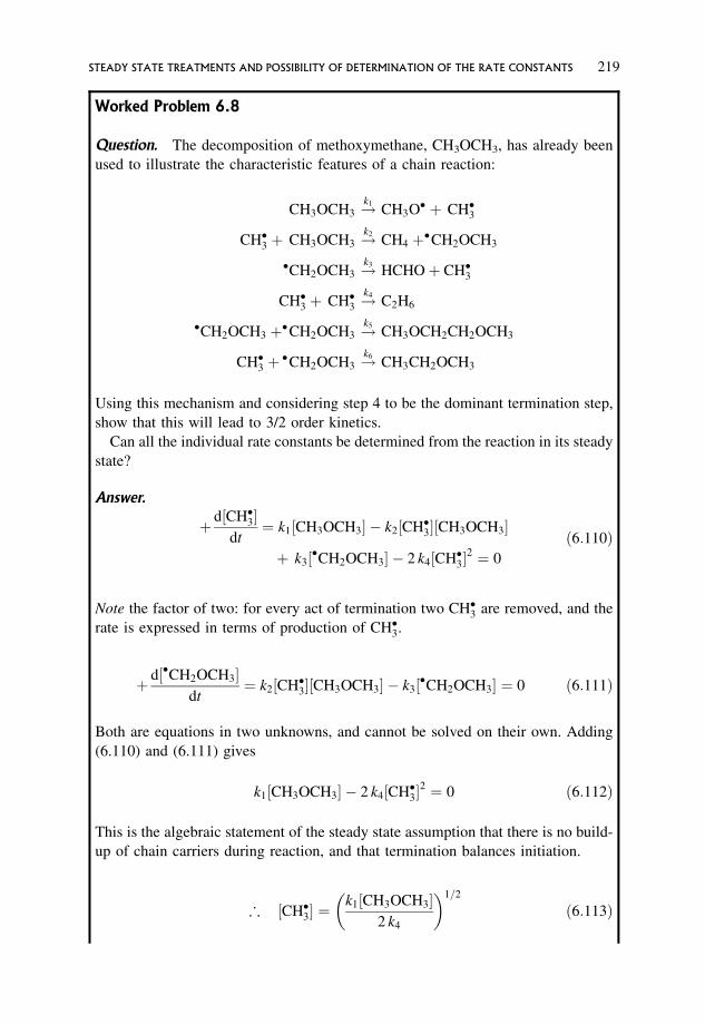
Worked Problem 6.8
Question. The decomposition of methoxymethane, CH3OCH3, has already been
used to illustrate the characteristic features of a chain reaction:
CH3OCH3 !k1
CH3O� þ CH�3
CH�3 þ CH3OCH3 !k2
CH4 þ�CH2OCH3
�CH2OCH3 !k3
HCHOþ CH�3
CH�3 þ CH�3 !k4
C2H6
�CH2OCH3 þ�CH2OCH3 !k5
CH3OCH2CH2OCH3
CH�3 þ�CH2OCH3 !k6
CH3CH2OCH3
Using this mechanism and considering step 4 to be the dominant termination step,
show that this will lead to 3/2 order kinetics.
Can all the individual rate constants be determined from the reaction in its steady
state?
Answer.
þ d½CH�3�dt
¼ k1½CH3OCH3� k2½CH�3�½CH3OCH3�
þ k3½�CH2OCH3� 2 k4½CH�3�2 ¼ 0
ð6:110Þ
Note the factor of two: for every act of termination two CH�3 are removed, and the
rate is expressed in terms of production of CH�3.
þ d½�CH2OCH3�dt
¼ k2½CH�3�½CH3OCH3� k3½�CH2OCH3� ¼ 0 ð6:111Þ
Both are equations in two unknowns, and cannot be solved on their own. Adding
(6.110) and (6.111) gives
k1½CH3OCH3� 2 k4½CH�3�2 ¼ 0 ð6:112Þ
This is the algebraic statement of the steady state assumption that there is no build-
up of chain carriers during reaction, and that termination balances initiation.
; ½CH�3� ¼k1½CH3OCH3�
2 k4
� �1=2
ð6:113Þ
STEADY STATE TREATMENTS AND POSSIBILITY OF DETERMINATION OF THE RATE CONSTANTS 219
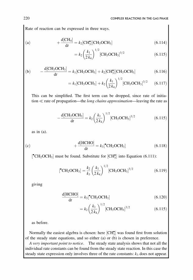
Rate of reaction can be expressed in three ways.
ðaÞ þ d½CH4�dt
¼ k2½CH�3�½CH3OCH3� ð6:114Þ
¼ k2
k1
2 k4
� �1=2
½CH3OCH3�3=2 ð6:115Þ
ðbÞ d½CH3OCH3�dt
¼ k1½CH3OCH3� þ k2½CH�3�½CH3OCH3� ð6:116Þ
¼ k1½CH3OCH3� þ k2
k1
2 k4
� �1=2
½CH3OCH3�3=2 ð6:117Þ
This can be simplified. The first term can be dropped, since rate of initia-
tion� rate of propagation—the long chains approximation—leaving the rate as
d½CH3OCH3�dt
¼ k2
k1
2 k4
� �1=2
½CH3OCH3�3=2 ð6:115Þ
as in (a).
ðcÞ þ d½HCHO�dt
¼ k3½�CH2OCH3� ð6:118Þ
½�CH2OCH3� must be found. Substitute for ½CH�3� into Equation (6.111):
½�CH2OCH3� ¼k2
k3
k1
2 k4
� �1=2
½CH3OCH3�3=2 ð6:119Þ
giving
d½HCHO�dt
¼ k3½�CH2OCH3� ð6:120Þ
¼ k2
k1
2 k4
� �1=2
½CH3OCH3�3=2 ð6:115Þ
as before.
Normally the easiest algebra is chosen: here ½CH�3� was found first from solution
of the steady state equations, and so either (a) or (b) is chosen in preference.
A very important point to notice. The steady state analysis shows that not all the
individual rate constants can be found from the steady state reaction. In this case the
steady state expression only involves three of the rate constants: k3 does not appear.
220 COMPLEX REACTIONS IN THE GAS PHASE
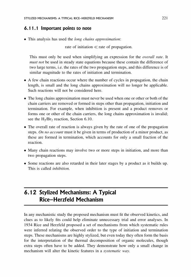
6.11.1 Important points to note
� This analysis has used the long chains approximation:
rate of initiation� rate of propagation.
This must only be used when simplifying an expression for the overall rate. It
must not be used in steady state equations because these contain the difference of
two large terms, i.e. the rates of the two propagation steps, and this difference is of
similar magnitude to the rates of initiation and termination.
� A few chain reactions occur where the number of cycles in propagation, the chain
length, is small and the long chains approximation will no longer be applicable.
Such reactions will not be considered here.
� The long chains approximation must never be used when one or other or both of the
chain carriers are removed or formed in steps other than propagation, initiation and
termination. For example, when inhibition is present and a product removes or
forms one or other of the chain carriers, the long chains approximation is invalid;
see the H2/Br2 reaction, Section 6.10.
� The overall rate of reaction is always given by the rate of one of the propagation
steps. On no account must it be given in terms of production of a minor product, as
these are formed in termination, which accounts for only a small fraction of the
reaction.
� Many chain reactions may involve two or more steps in initiation, and more than
two propagation steps.
� Some reactions are also retarded in their later stages by a product as it builds up.
This is called inhibition.
6.12 Stylized Mechanisms: A Typical
Rice–Herzfeld Mechanism
In any mechanistic study the proposed mechanism must fit the observed kinetics, and
clues as to likely fits could help eliminate unnecessary trial and error analyses. In
1934 Rice and Herzfeld proposed a set of mechanisms from which systematic rules
were inferred relating the observed order to the type of initiation and termination
steps. These mechanisms are highly stylized, but even today they often form the basis
for the interpretation of the thermal decomposition of organic molecules, though
extra steps often have to be added. They demonstrate how only a small change in
mechanism will alter the kinetic features in a systematic way.
STYLIZED MECHANISMS: A TYPICAL RICE–HERZFELD MECHANISM 221

The overall reaction considered is
X! P1 þ P2
However, minor products, P3, P4 and P5 are also formed, along with radical
intermediates R�, R�1, and R�2. A possible schematic mechanism is
Xþ ðMÞ !k1R� þ R�1 þ ðMÞ initiation
R�1 þ X !k2R�2 þ P1 propagation
R�2 þ ðMÞ !k3
R�1 þ P2 þ ðMÞ propagation
R�1 þ R�1 þ ðMÞ !k4
P3 þ ðMÞ termination
R�2 þ R�2 þ ðMÞ !k5
P4 þ ðMÞ termination
R�1 þ R�2 þ ðMÞ !k6
P5 þ ðMÞ termination
R� is formed in initiation, but as it is not involved in propagation it is not a chain
carrier and will be removed in some subsequent reaction not associated with the
chain. M is a third body whose significance will be explained below (Section 6.12.4).
A steady state treatment shows the overall order to depend on the type of step in
which the radical is formed, and also on which termination step is dominant.
R�1 þ R�1 recombination ! 3/2 order: R�1 is formed in initiation, used in the first
propagation step and re-formed in the second.
R�2 þ R�2 recombination! 1/2 order: R�2 is formed in the first propagation step and
is used in the second.
R�1 þ R�2 recombination ! first order.
This treatment can be extended to include various types of initiation and propaga-
tion steps, and a whole systematic classification built up whereby the overall order
can be predicted for any set of initiation, propagation and termination steps.
Several points can be made about this mechanism:
� Initiation is unimolecular, showing first order kinetics at high pressures where the
reaction step is rate determining, moving to the low pressure second order region
where activation is rate determining (see Chapter 1 and Section 4.5). The reaction
step referred to here is that in the physical mechanism of an elementary step:
Aþ A! A þ A collisional activation step
A þ A! Aþ A collisional deactivation step
A þ bA! products reaction step
where b ¼ 0 when reaction is unimolecular and b ¼ 1 when reaction is bimolecular.
222 COMPLEX REACTIONS IN THE GAS PHASE
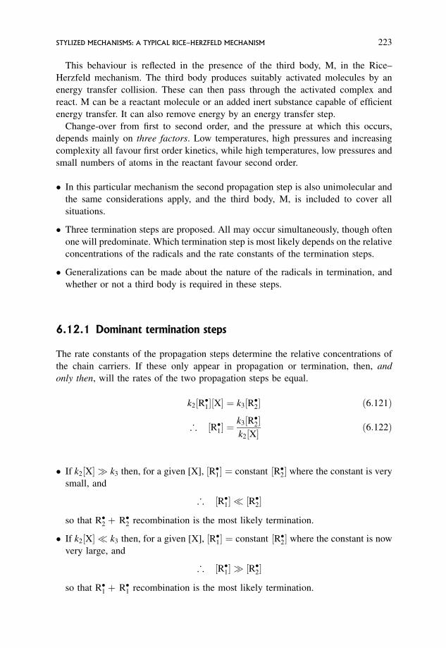
This behaviour is reflected in the presence of the third body, M, in the Rice–
Herzfeld mechanism. The third body produces suitably activated molecules by an
energy transfer collision. These can then pass through the activated complex and
react. M can be a reactant molecule or an added inert substance capable of efficient
energy transfer. It can also remove energy by an energy transfer step.
Change-over from first to second order, and the pressure at which this occurs,
depends mainly on three factors. Low temperatures, high pressures and increasing
complexity all favour first order kinetics, while high temperatures, low pressures and
small numbers of atoms in the reactant favour second order.
� In this particular mechanism the second propagation step is also unimolecular and
the same considerations apply, and the third body, M, is included to cover all
situations.
� Three termination steps are proposed. All may occur simultaneously, though often
one will predominate. Which termination step is most likely depends on the relative
concentrations of the radicals and the rate constants of the termination steps.
� Generalizations can be made about the nature of the radicals in termination, and
whether or not a third body is required in these steps.
6.12.1 Dominant termination steps
The rate constants of the propagation steps determine the relative concentrations of
the chain carriers. If these only appear in propagation or termination, then, and
only then, will the rates of the two propagation steps be equal.
k2½R�1�½X� ¼ k3½R�2� ð6:121Þ
; ½R�1� ¼k3½R�2�k2½X�
ð6:122Þ
� If k2½X� � k3 then, for a given [X], ½R�1� ¼ constant ½R�2� where the constant is very
small, and
; ½R�1� � ½R�2�
so that R�2 þ R�2 recombination is the most likely termination.
� If k2½X� � k3 then, for a given [X], ½R�1� ¼ constant ½R�2� where the constant is now
very large, and
; ½R�1� � ½R�2�
so that R�1 þ R�1 recombination is the most likely termination.
STYLIZED MECHANISMS: A TYPICAL RICE–HERZFELD MECHANISM 223
� If k2½X� is comparable to k3, then ½R�1� and ½R�2� are comparable. Discrimination as
to which termination step is most likely is impossible. In this situation the relative
rate constants of the termination steps are the major influence.
6.12.2 Relative rate constants for termination steps
Transition state theory (Section 4.4) gives the rate constant
k ¼ �kT
hexp
þ�S6¼
R
� �exp
�H 6¼
RT
� �ð4:41Þ
where �H 6¼, the change in enthalpy on forming the activated complex, is closely
related to the activation energy. �S 6¼ is the entropy of activation.
Radical recombinations have zero, or small positive or negative activation energies,
and so to a first approximation
k ¼ �kT
hexp
þ�S6¼
R
� �ð6:123Þ
for these reactions.
Since �kT=h is a constant, then the rate constant for each termination step reflects
the magnitude and sign of the entropy of activation.
�S6¼ is the entropy of activation, i.e. the change in entropy for the process of
reactants moving into the activated complex. In the gas phase it is governed by the
change in the number and types of degrees of freedom on activation, these degrees of
freedom being related to translations, rotations and vibrations. Calculations show that
reactions between large complex radicals have large negative �S6¼, so
expðþ�S6¼=RÞ is very small, resulting in a small rate constant. Conversely, for
small, simple radicals, �S6¼ is considerably less negative and their rate constants are
much higher than for large radicals (see Sections 4.4.2 and 4.4.3 and Worked
Problems 4.15 and 4.16).
6.12.3 Relative rates of the termination steps
In practice these are a function of both the chain carrier concentrations and the rate
constants for termination. Specific predictions can only be made if all rate constants
for propagation and termination are known. It is only when the chain carrier
concentrations are comparable that it is possible to say that reactions between the
smaller radicals will dominate.
224 COMPLEX REACTIONS IN THE GAS PHASE
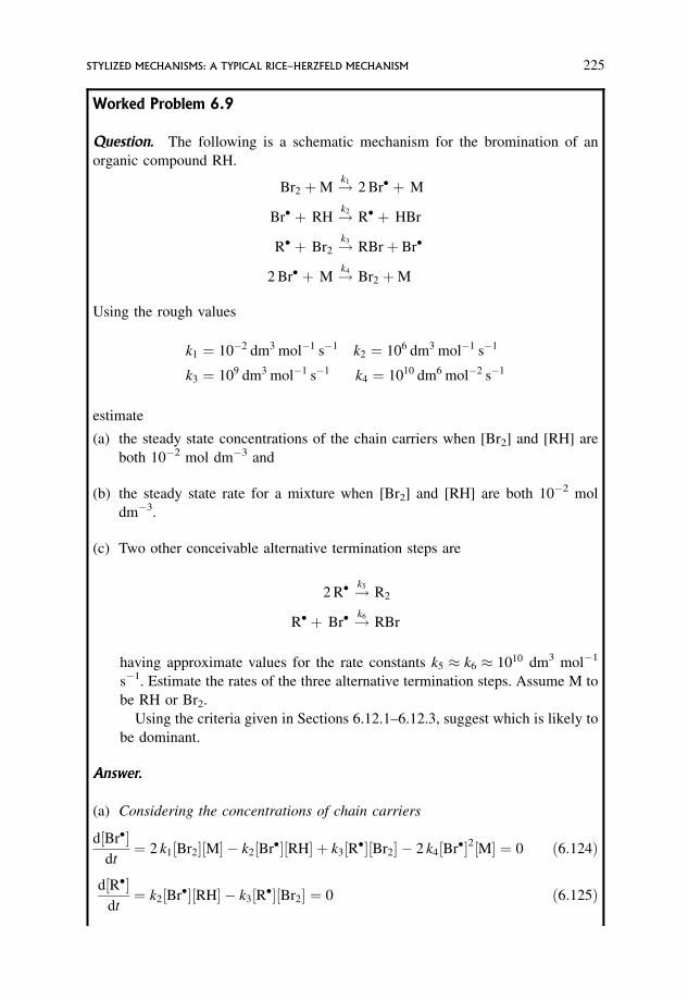
Worked Problem 6.9
Question. The following is a schematic mechanism for the bromination of an
organic compound RH.
Br2 þM !k12 Br� þ M
Br� þ RH !k2R� þ HBr
R� þ Br2 !k3
RBrþ Br�
2 Br� þ M !k4Br2 þM
Using the rough values
k1 ¼ 102 dm3 mol1 s1 k2 ¼ 106 dm3 mol1 s1
k3 ¼ 109 dm3 mol1 s1 k4 ¼ 1010 dm6 mol2 s1
estimate
(a) the steady state concentrations of the chain carriers when [Br2] and [RH] are
both 102 mol dm3 and
(b) the steady state rate for a mixture when [Br2] and [RH] are both 102 mol
dm3.
(c) Two other conceivable alternative termination steps are
2 R� !k5R2
R� þ Br� !k6RBr
having approximate values for the rate constants k5 � k6 � 1010 dm3 mol1
s1. Estimate the rates of the three alternative termination steps. Assume M to
be RH or Br2.
Using the criteria given in Sections 6.12.1–6.12.3, suggest which is likely to
be dominant.
Answer.
(a) Considering the concentrations of chain carriers
d½Br��dt¼ 2 k1½Br2�½M� k2½Br��½RH� þ k3½R��½Br2� 2 k4½Br��2½M� ¼ 0 ð6:124Þ
d½R��dt¼ k2½Br��½RH� k3½R��½Br2� ¼ 0 ð6:125Þ
STYLIZED MECHANISMS: A TYPICAL RICE–HERZFELD MECHANISM 225
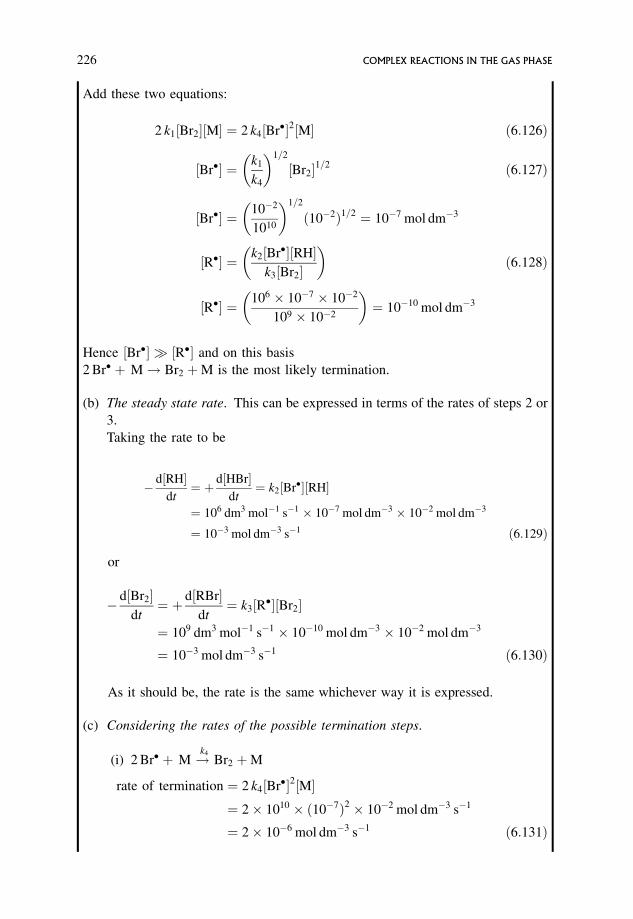
Add these two equations:
2 k1½Br2�½M� ¼ 2 k4½Br��2½M� ð6:126Þ
½Br�� ¼ k1
k4
� �1=2
½Br2�1=2 ð6:127Þ
½Br�� ¼ 102
1010
� �1=2
ð102Þ1=2 ¼ 107 mol dm3
½R�� ¼ k2½Br��½RH�k3½Br2�
� �ð6:128Þ
½R�� ¼ 106 � 107 � 102
109 � 102
� �¼ 1010 mol dm3
Hence ½Br�� � ½R�� and on this basis
2 Br� þ M! Br2 þM is the most likely termination.
(b) The steady state rate. This can be expressed in terms of the rates of steps 2 or
3.
Taking the rate to be
d½RH�dt¼ þ d½HBr�
dt¼ k2½Br��½RH�
¼ 106 dm3 mol1 s1 � 107 mol dm3 � 102 mol dm3
¼ 103 mol dm3 s1 ð6:129Þ
or
d½Br2�dt¼ þ d½RBr�
dt¼ k3½R��½Br2�
¼ 109 dm3 mol1 s1 � 1010 mol dm3 � 102 mol dm3
¼ 103 mol dm3 s1 ð6:130Þ
As it should be, the rate is the same whichever way it is expressed.
(c) Considering the rates of the possible termination steps.
(i) 2 Br� þ M !k4
Br2 þM
rate of termination ¼ 2 k4½Br��2½M�¼ 2� 1010 � ð107Þ2 � 102 mol dm3 s1
¼ 2� 106 mol dm3 s1 ð6:131Þ
226 COMPLEX REACTIONS IN THE GAS PHASE
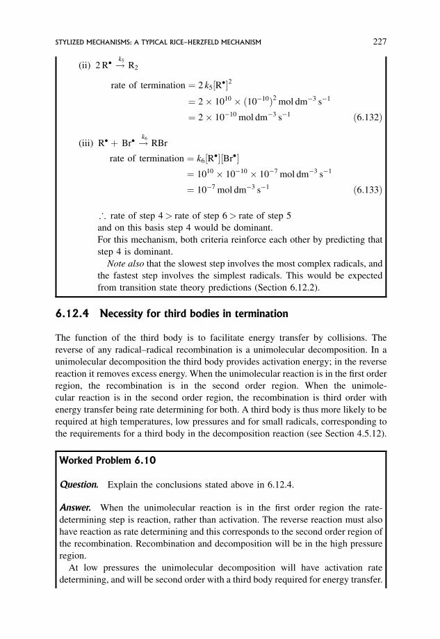
(ii) 2 R� !k5
R2
rate of termination ¼ 2 k5½R��2
¼ 2� 1010 � ð1010Þ2 mol dm3 s1
¼ 2� 1010 mol dm3 s1 ð6:132Þ
(iii) R� þ Br� !k6
RBr
rate of termination ¼ k6½R��½Br��¼ 1010 � 1010 � 107 mol dm3 s1
¼ 107 mol dm3 s1 ð6:133Þ
; rate of step 4 > rate of step 6 > rate of step 5
and on this basis step 4 would be dominant.
For this mechanism, both criteria reinforce each other by predicting that
step 4 is dominant.
Note also that the slowest step involves the most complex radicals, and
the fastest step involves the simplest radicals. This would be expected
from transition state theory predictions (Section 6.12.2).
6.12.4 Necessity for third bodies in termination
The function of the third body is to facilitate energy transfer by collisions. The
reverse of any radical–radical recombination is a unimolecular decomposition. In a
unimolecular decomposition the third body provides activation energy; in the reverse
reaction it removes excess energy. When the unimolecular reaction is in the first order
region, the recombination is in the second order region. When the unimole-
cular reaction is in the second order region, the recombination is third order with
energy transfer being rate determining for both. A third body is thus more likely to be
required at high temperatures, low pressures and for small radicals, corresponding to
the requirements for a third body in the decomposition reaction (see Section 4.5.12).
Worked Problem 6.10
Question. Explain the conclusions stated above in 6.12.4.
Answer. When the unimolecular reaction is in the first order region the rate-
determining step is reaction, rather than activation. The reverse reaction must also
have reaction as rate determining and this corresponds to the second order region of
the recombination. Recombination and decomposition will be in the high pressure
region.
At low pressures the unimolecular decomposition will have activation rate
determining, and will be second order with a third body required for energy transfer.
STYLIZED MECHANISMS: A TYPICAL RICE–HERZFELD MECHANISM 227
The recombination must also have energy transfer as rate determining, and for this
removal of energy a third body is required, leading to third order kinetics (see
Section 4.5.12).
These generalizations about the need for a third body can be explained physically
in terms of the three types of recombination:
R�1 and R�2 are atoms;
R�1 and R�2 are large radicals;
R�1 and R�2 are small radicals:
� R�1 and R�2 are atoms. When atoms recombine, the energy resulting from the
highly exothermic reaction initially resides in the newly formed bond which is thus
highly excited. If this energy is not removed before the first vibration occurs, then
the diatomic molecule will dissociate on vibration and effective recombination will
not occur. This energy can only be removed by a collision, which must occur in a
time less than the time for one vibration. A third body is required, and can be either
the reactant or another molecule capable of efficient energy transfer.
Aþ A! A2 an excited diatomic molecule
Mþ A2 ! A2 þM an energy transfer collision
Third bodies are thus required for atom–atom recombinations.
� R�1 and R�2 are large radicals. These form a high energy complex molecule with
the exothermicity of the recombination residing in the newly formed bond. This
energy has to be removed before the bond executes a vibration. However, for large
polyatomic molecules with a large number of vibrational modes there is an
alternative route for stabilizing the newly formed bond. Because of anharmonicity,
the excess energy can be distributed very, very rapidly around the molecule via the
normal modes of vibration. The molecule, as a whole, is still highly excited, but the bond
is stabilized before it has time to dissociate. This can be achieved in a time short
compared to that for a vibration. This increases the lifetime of the excited molecule and
the normal process of energy transfer by collision can occur after many vibrations of the
bond. Third bodies are thus not required for large radical recombinations.
� R�1 and R�2 are small radicals. If the radical is small then the molecule may not
have enough normal modes into which the excess energy can be channelled, and a
third body will be necessary. As the radical size increases many more normal
modes become available, and the chances of the bond being stabilized rapidly
increase, reducing the need for a third body. The minimum number of normal
modes required for adequate stabilization of the newly formed bond depends also
on the temperature and pressure. If the number of normal modes exceeds around
ten then a third body probably is not needed, provided the pressure is high enough.
When the number is between six and ten there is a high chance that a third body
will be required, and again the pressure may well prove decisive.
228 COMPLEX REACTIONS IN THE GAS PHASE
Worked Problem 6.11
Question. Predict whether a third body would be required in the following
recombinations. State whether any provisos should be made on pressure and
temperature considerations.
ðaÞ H� þ H� ! H2 ðbÞ H� þ OH� ! H2O
ðcÞ CH�3 þ Cl� ! CH3Cl ðdÞ CH�3 þ CH�3 ! C2H6
ðeÞ CH�3 þ C2H�5 ! C3H8 ðfÞ C3H�7 þ C3H�7 ! C6H14
Answer.
(a) Two atoms recombining: third body always required.
(b) Atomþ small radical recombining; non-linear triatomic molecule formed;
3 N 6 ¼ 3 vibrations: third body normally required.
(c) As in (b), but here the non-linear product has five atoms, i.e. ninevibrations. The third
body possibly might not be required unless the pressure is low and the temperature is
high. The reverse decomposition would then be expected to be second order under
these conditions and require a third body in the activation step. This has been
observed.
(d) As in (c), but eight atoms in product, i.e. 18 vibrations with conclusions similar
to (c). At very low pressures and high temperatures a third body is required for
the activation step. The reverse decomposition has been observed to move from first
order towards second as the pressure is lowered, and so under these conditions of
pressure the recombination would be third order, i.e. a third body is required.
(e) The product of (e) has 11 atoms and 27 vibrations. Although this has a fairly
large number of normal modes of vibration and a third body would normally
not be required, this reaction might still need a third body at very low pressures
and high temperatures.
(f) The product of (f) has 20 atoms and 54 vibrations, and a third body
requirement is not expected.
The results for (d) and (e) illustrate that, although a third body is not required under
normal experimental conditions and the normal modes can cope with stabilizing the
newly formed bond, this will not necessarily hold as the pressure is lowered.
This means that there is a range of sizes of the recombining radicals where there
may be pressure and temperature regions where even a relatively large number of
normal modes of vibration may not be enough to stabilize the newly formed bond.
6.12.5 The steady state treatment for chain reactions, illustrating
the use of the long chains approximation
A simplified mechanism for the oxidation of hydrocarbons can be given. Such
reactions often involve an initiator, I. This is a molecule which by decomposing
STYLIZED MECHANISMS: A TYPICAL RICE–HERZFELD MECHANISM 229
produces a radical, X�. This, in turn, reacts with O2 to produce a peroxy radical, XO�2,
which can then set the chain process going by producing the radical, R�.One possible mechanism is
I !k1X� þ R0�
X� þ O2 !k2
XO�2
XO�2 þ RH !k3XOOHþ R�
9>>>=>>>;
three stage initiation
R� þ O2 !k4
RO�2
RO�2 þ RH !k5ROOHþ R�
9=;propagation
RO�2 þ RO�2 !k6
inert moleculeþ O2 termination
This is a highly simplified mechanism, but it does contain the essentials of the main
chain process. This mechanism involves a three stage initiation process, something
not uncommon in chain mechanisms. Only one of the possible propagation chains is
given, and only one termination step is quoted.
The chain carriers are R� and RO�2, and the major product is ROOH. There are two
radical intermediates, X� and XO�2, in this reaction which are not chain carriers, but
are necessary for the production of the chain carriers. They must, therefore, be
included in the steady state treatment. However, R0�, though a radical, is not involved
in any chain and so does not come into the steady state treatment.
The steady state treatment is
d½X��dt¼ k1½I� k2½X��½O2� ¼ 0 ð6:134Þ
d½XO�2�dt
¼ k2½X��½O2� k3½XO�2�½RH� ¼ 0 ð6:135Þ
d½R��dt¼ k3½XO�2�½RH� k4½R��½O2� þ k5½RO�2�½RH� ¼ 0 ð6:136Þ
d½RO�2�dt
¼ k4½R��½O2� k5½RO�2�½RH� 2 k6½RO�2�2 ¼ 0 ð6:137Þ
The standard procedure is to add all the steady state equations. This gives
k1½I� ¼ 2 k6½RO�2�2 ð6:138Þ
; ½RO�2� ¼k1
2 k6
� �1=2
½I�1=2 ð6:139Þ
230 COMPLEX REACTIONS IN THE GAS PHASE
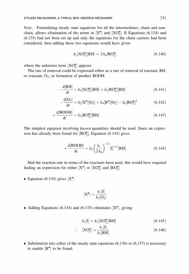
Note. Formulating steady state equations for all the intermediates, chain and non-
chain, allows elimination of the terms in ½X�� and ½XO�2�. If Equations (6.134) and
(6.135) had not been set up and only the equations for the chain carriers had been
considered, then adding these two equations would have given
k3½XO�2�½RH� ¼ 2 k6½RO�2� ð6:140Þ
where the unknown term ½XO�2� appears.
The rate of removal could be expressed either as a rate of removal of reactant, RH,
or reactant, O2, or formation of product ROOH.
d½RH�dt¼ k3½XO�2�½RH� þ k5½RO�2�½RH� ð6:141Þ
d½O2�dt¼ k2½X��½O2� þ k4½R��½O2� k6½RO�2�
2 ð6:142Þ
þ d½ROOH�dt
¼ k5½RO�2�½RH� ð6:143Þ
The simplest equation involving known quantities should be used. Since an expres-
sion has already been found for ½RO�2�, Equation (6.143) gives
þ d½ROOH�dt
¼ k5
k1
2 k6
� �1=2
½I�1=2½RH� ð6:144Þ
Had the reaction rate in terms of the reactants been used, this would have required
finding an expression for either ½X�� or ½XO�2� and ½RO�2�.
� Equation (6.134) gives ½X��
½X�� ¼ k1½I�k2½O2�
� Adding Equations (6.134) and (6.135) eliminates ½X��, giving
k1½I� ¼ k3½XO�2�½RH� ð6:145Þ
; ½XO�2� ¼k1½I�
k3½RH� ð6:146Þ
� Substitution into either of the steady state equations (6.136) or (6.137) is necessary
to enable ½R�� to be found.
STYLIZED MECHANISMS: A TYPICAL RICE–HERZFELD MECHANISM 231
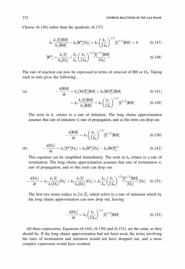
Choose (6.136) rather than the quadratic (6.137)
k3
k1½I�½RH�k3½RH� k4½R��½O2� þ k5
k1
2 k6
� �1=2
½I�1=2½RH� ¼ 0 ð6:147Þ
½R�� ¼ k1½I�k4½O2�
þ k5
k4
k1
2 k6
� �1=2½I�1=2½RH�½O2�
ð6:148Þ
The rate of reaction can now be expressed in terms of removal of RH or O2. Taking
each in turn gives the following.
(a) d½RH�dt¼ k3½XO�2�½RH� þ k5½RO�2�½RH� ð6:141Þ
¼ k3
k1½I�½RH�k3½RH� þ k5
k1
2 k6
� �1=2
½I�1=2½RH� ð6:149Þ
The term in k1 relates to a rate of initiation. The long chains approximation
assumes that rate of initiation� rate of propagation, and so this term can drop out.
d½RH�dt¼ k5
k1
2 k6
� �1=2
½I�1=2½RH� ð6:150Þ
(b) d½O2�dt¼ k2½X��½O2� þ k4½R��½O2� k6½RO�2�
2 ð6:142Þ
This equation can be simplified immediately. The term in k6 relates to a rate of
termination. The long chains approximation assumes that rate of termination�rate of propagation, and so this term can drop out.
d½O2�dt¼ k2
k1½I�k2½O2�
½O2� þ k4
k1½I�k4½O2�
½O2� þ k4
k5
k4
k1
2 k6
� �1=2½I�1=2½RH�½O2�
½O2� ð6:151Þ
The first two terms reduce to 2 k1½I�, which refers to a rate of initiation which by
the long chains approximation can now drop out, leaving
d½O2�dt¼ k5
k1
2 k6
� �1=2
½I�1=2½RH� ð6:152Þ
All three expressions, Equations (6.144), (6.150) and (6.152), are the same, as they
should be. If the long chains approximation had not been used, the terms involving
the rates of termination and initiation would not have dropped out, and a more
complex expression would have resulted.
232 COMPLEX REACTIONS IN THE GAS PHASE
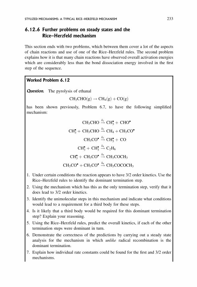
6.12.6 Further problems on steady states and the
Rice–Herzfeld mechanism
This section ends with two problems, which between them cover a lot of the aspects
of chain reactions and use of one of the Rice–Herzfeld rules. The second problem
explains how it is that many chain reactions have observed overall activation energies
which are considerably less than the bond dissociation energy involved in the first
step of the sequence.
Worked Problem 6.12
Question. The pyrolysis of ethanal
CH3CHOðgÞ ! CH4ðgÞ þ COðgÞ
has been shown previously, Problem 6.7, to have the following simplified
mechanism:
CH3CHO !k1CH�3 þ CHO�
CH�3 þ CH3CHO !k2CH4 þ CH3CO�
CH3CO� !k3CH�3 þ CO
CH�3 þ CH�3 !k4
C2H6
CH�3 þ CH3CO� !k5CH3COCH3
CH3CO� þ CH3CO� !k6CH3COCOCH3
1. Under certain conditions the reaction appears to have 3/2 order kinetics. Use the
Rice–Herzfeld rules to identify the dominant termination step.
2. Using the mechanism which has this as the only termination step, verify that it
does lead to 3/2 order kinetics.
3. Identify the unimolecular steps in this mechanism and indicate what conditions
would lead to a requirement for a third body for these steps.
4. Is it likely that a third body would be required for this dominant termination
step? Explain your reasoning.
5. Using the Rice–Herzfeld rules, predict the overall kinetics, if each of the other
termination steps were dominant in turn.
6. Demonstrate the correctness of the predictions by carrying out a steady state
analysis for the mechanism in which unlike radical recombination is the
dominant termination.
7. Explain how individual rate constants could be found for the first and 3/2 order
mechanisms.
STYLIZED MECHANISMS: A TYPICAL RICE–HERZFELD MECHANISM 233
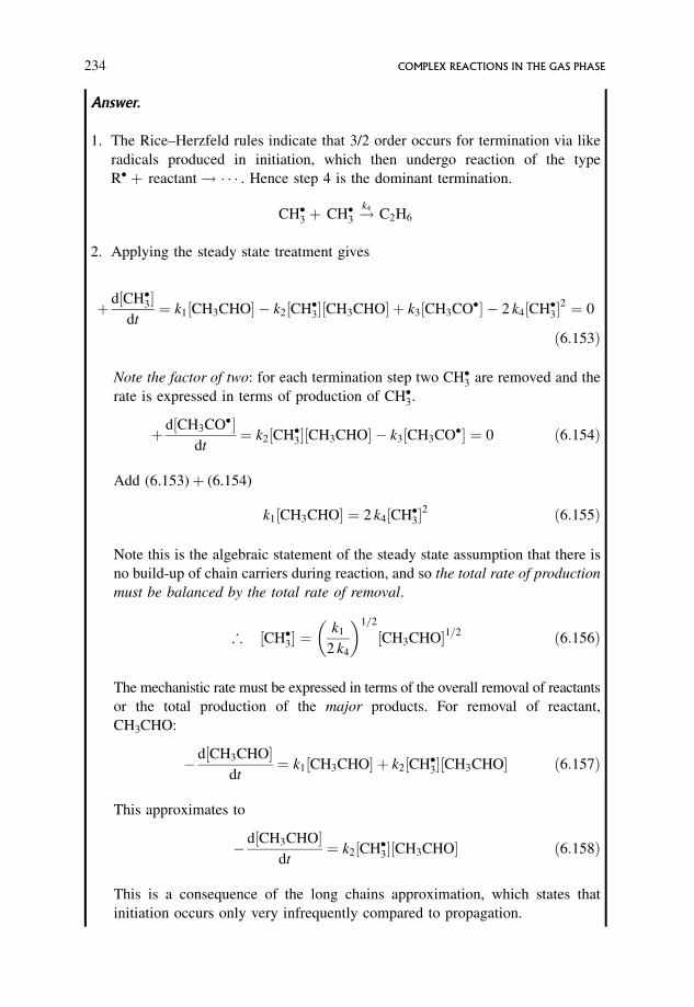
Answer.
1. The Rice–Herzfeld rules indicate that 3/2 order occurs for termination via like
radicals produced in initiation, which then undergo reaction of the type
R� þ reactant! � � � . Hence step 4 is the dominant termination.
CH�3 þ CH�3 !k4
C2H6
2. Applying the steady state treatment gives
þ d½CH�3�dt
¼ k1½CH3CHO� k2½CH�3�½CH3CHO� þ k3½CH3CO�� 2 k4½CH�3�2 ¼ 0
ð6:153Þ
Note the factor of two: for each termination step two CH�3 are removed and the
rate is expressed in terms of production of CH�3.
þ d½CH3CO��dt
¼ k2½CH�3�½CH3CHO� k3½CH3CO�� ¼ 0 ð6:154Þ
Add (6.153)þ (6.154)
k1½CH3CHO� ¼ 2 k4½CH�3�2 ð6:155Þ
Note this is the algebraic statement of the steady state assumption that there is
no build-up of chain carriers during reaction, and so the total rate of production
must be balanced by the total rate of removal.
; ½CH�3� ¼k1
2 k4
� �1=2
½CH3CHO�1=2 ð6:156Þ
The mechanistic rate must be expressed in terms of the overall removal of reactants
or the total production of the major products. For removal of reactant,
CH3CHO:
d½CH3CHO�dt
¼ k1½CH3CHO� þ k2½CH�3�½CH3CHO� ð6:157Þ
This approximates to
d½CH3CHO�dt
¼ k2½CH�3�½CH3CHO� ð6:158Þ
This is a consequence of the long chains approximation, which states that
initiation occurs only very infrequently compared to propagation.
234 COMPLEX REACTIONS IN THE GAS PHASE
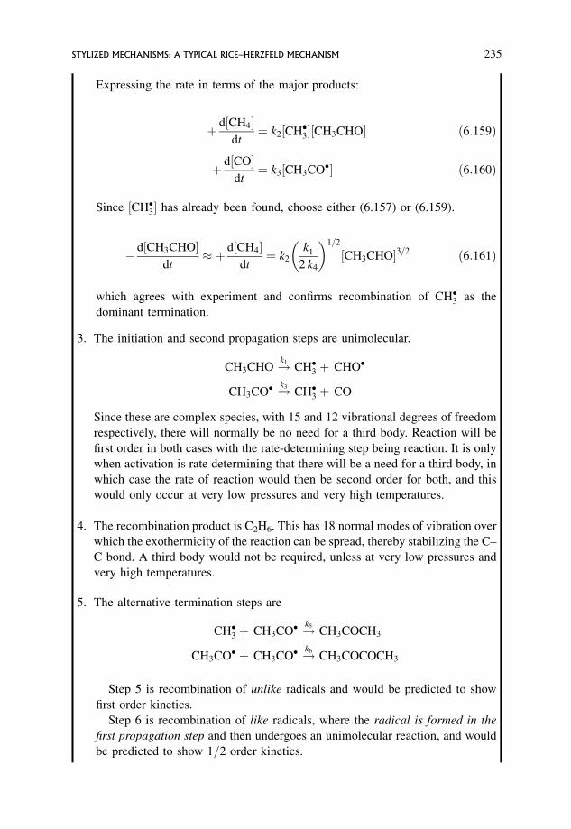
Expressing the rate in terms of the major products:
þ d½CH4�dt
¼ k2½CH�3�½CH3CHO� ð6:159Þ
þ d½CO�dt¼ k3½CH3CO�� ð6:160Þ
Since ½CH�3� has already been found, choose either (6.157) or (6.159).
d½CH3CHO�dt
� þ d½CH4�dt
¼ k2
k1
2 k4
� �1=2
½CH3CHO�3=2 ð6:161Þ
which agrees with experiment and confirms recombination of CH�3 as the
dominant termination.
3. The initiation and second propagation steps are unimolecular.
CH3CHO !k1CH�3 þ CHO�
CH3CO� !k3CH�3 þ CO
Since these are complex species, with 15 and 12 vibrational degrees of freedom
respectively, there will normally be no need for a third body. Reaction will be
first order in both cases with the rate-determining step being reaction. It is only
when activation is rate determining that there will be a need for a third body, in
which case the rate of reaction would then be second order for both, and this
would only occur at very low pressures and very high temperatures.
4. The recombination product is C2H6. This has 18 normal modes of vibration over
which the exothermicity of the reaction can be spread, thereby stabilizing the C–
C bond. A third body would not be required, unless at very low pressures and
very high temperatures.
5. The alternative termination steps are
CH�3 þ CH3CO� !k5CH3COCH3
CH3CO� þ CH3CO� !k6CH3COCOCH3
Step 5 is recombination of unlike radicals and would be predicted to show
first order kinetics.
Step 6 is recombination of like radicals, where the radical is formed in the
first propagation step and then undergoes an unimolecular reaction, and would
be predicted to show 1=2 order kinetics.
STYLIZED MECHANISMS: A TYPICAL RICE–HERZFELD MECHANISM 235
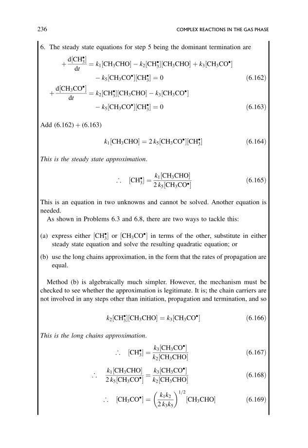
6. The steady state equations for step 5 being the dominant termination are
þ d½CH�3�dt
¼ k1½CH3CHO� k2½CH�3�½CH3CHO� þ k3½CH3CO��
k5½CH3CO��½CH�3� ¼ 0 ð6:162Þ
þ d½CH3CO��dt
¼ k2½CH�3�½CH3CHO� k3½CH3CO��
k5½CH3CO��½CH�3� ¼ 0 ð6:163Þ
Add (6.162)þ (6.163)
k1½CH3CHO� ¼ 2 k5½CH3CO��½CH�3� ð6:164Þ
This is the steady state approximation.
; ½CH�3� ¼k1½CH3CHO�2 k5½CH3CO�� ð6:165Þ
This is an equation in two unknowns and cannot be solved. Another equation is
needed.
As shown in Problems 6.3 and 6.8, there are two ways to tackle this:
(a) express either ½CH�3� or ½CH3CO�� in terms of the other, substitute in either
steady state equation and solve the resulting quadratic equation; or
(b) use the long chains approximation, in the form that the rates of propagation are
equal.
Method (b) is algebraically much simpler. However, the mechanism must be
checked to see whether the approximation is legitimate. It is; the chain carriers are
not involved in any steps other than initiation, propagation and termination, and so
k2½CH�3�½CH3CHO� ¼ k3½CH3CO�� ð6:166Þ
This is the long chains approximation.
; ½CH�3� ¼k3½CH3CO��k2½CH3CHO� ð6:167Þ
;k1½CH3CHO�2 k5½CH3CO�� ¼
k3½CH3CO��k2½CH3CHO� ð6:168Þ
; ½CH3CO�� ¼ k1k2
2 k3k5
� �1=2
½CH3CHO� ð6:169Þ
236 COMPLEX REACTIONS IN THE GAS PHASE
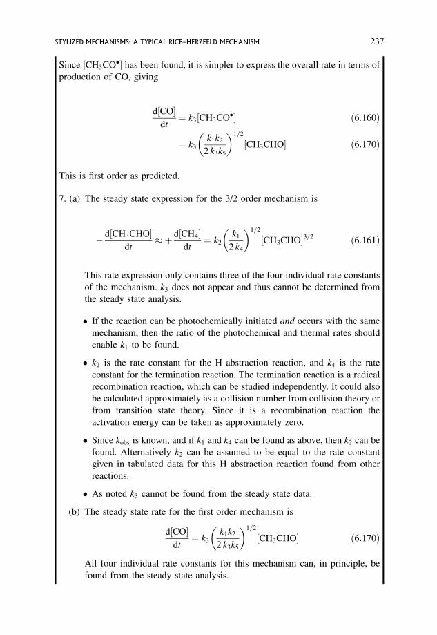
Since ½CH3CO�� has been found, it is simpler to express the overall rate in terms of
production of CO, giving
d½CO�dt¼ k3½CH3CO�� ð6:160Þ
¼ k3
k1k2
2 k3k5
� �1=2
½CH3CHO� ð6:170Þ
This is first order as predicted.
7. (a) The steady state expression for the 3/2 order mechanism is
d½CH3CHO�dt
� þ d½CH4�dt
¼ k2
k1
2 k4
� �1=2
½CH3CHO�3=2 ð6:161Þ
This rate expression only contains three of the four individual rate constants
of the mechanism. k3 does not appear and thus cannot be determined from
the steady state analysis.
� If the reaction can be photochemically initiated and occurs with the same
mechanism, then the ratio of the photochemical and thermal rates should
enable k1 to be found.
� k2 is the rate constant for the H abstraction reaction, and k4 is the rate
constant for the termination reaction. The termination reaction is a radical
recombination reaction, which can be studied independently. It could also
be calculated approximately as a collision number from collision theory or
from transition state theory. Since it is a recombination reaction the
activation energy can be taken as approximately zero.
� Since kobs is known, and if k1 and k4 can be found as above, then k2 can be
found. Alternatively k2 can be assumed to be equal to the rate constant
given in tabulated data for this H abstraction reaction found from other
reactions.
� As noted k3 cannot be found from the steady state data.
(b) The steady state rate for the first order mechanism is
d½CO�dt¼ k3
k1k2
2 k3k5
� �1=2
½CH3CHO� ð6:170Þ
All four individual rate constants for this mechanism can, in principle, be
found from the steady state analysis.
STYLIZED MECHANISMS: A TYPICAL RICE–HERZFELD MECHANISM 237
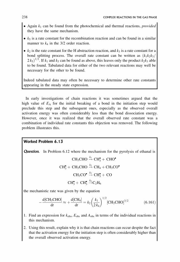
� Again k1 can be found from the photochemical and thermal reactions, provided
they have the same mechanism.
� k5 is a rate constant for the recombination reaction and can be found in a similar
manner to k4 in the 3/2 order reaction.
� k2 is the rate constant for the H abstraction reaction, and k3 is a rate constant for a
bond splitting process. The overall rate constant can be written as k1k2k3=ð2 k5Þ1=2
. If k1 and k5 can be found as above, this leaves only the product k2k3 able
to be found. Tabulated data for either of the two relevant reactions may well be
necessary for the other to be found.
Indeed tabulated data may often be necessary to determine other rate constants
appearing in the steady state expression.
In early investigations of chain reactions it was sometimes argued that the
high value of EA for the initial breaking of a bond in the initiation step would
preclude this step and the subsequent ones, especially as the observed overall
activation energy was often considerably less than the bond dissociation energy.
However, once it was realized that the overall observed rate constant was a
combination of individual rate constants this objection was removed. The following
problem illustrates this.
Worked Problem 6.13
Question. In Problem 6.12 where the mechanism for the pyrolysis of ethanal is
CH3CHO !k1CH�3 þ CHO�
CH�3 þ CH3CHO !k2CH4 þ CH3CO�
CH3CO� !k3CH�3 þ CO
CH�3 þ CH�3 !k4
C2H6
the mechanistic rate was given by the equation
d½CH3CHO�dt
� þ d½CH4�dt
¼ k2
k1
2 k4
� �1=2
½CH3CHO�3=2 ð6:161Þ
1. Find an expression for kobs, Eobs and Aobs in terms of the individual reactions in
this mechanism.
2. Using this result, explain why it is that chain reactions can occur despite the fact
that the activation energy for the initiation step is often considerably higher than
the overall observed activation energy.
238 COMPLEX REACTIONS IN THE GAS PHASE
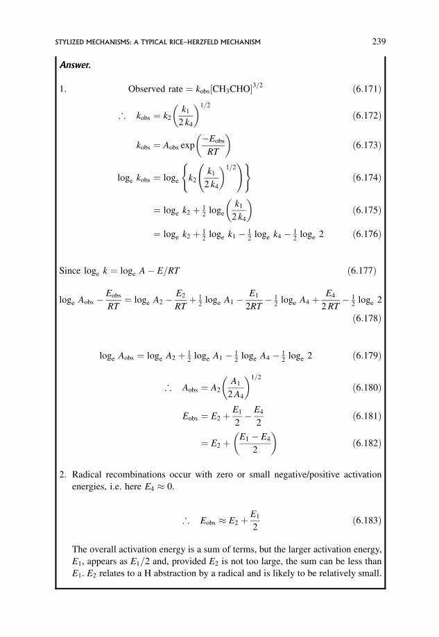
Answer.
1. Observed rate ¼ kobs½CH3CHO�3=2 ð6:171Þ
; kobs ¼ k2
k1
2 k4
� �1=2
ð6:172Þ
kobs ¼ Aobs expEobs
RT
� �ð6:173Þ
loge kobs ¼ loge k2
k1
2 k4
�1=2 !( )
ð6:174Þ
¼ loge k2 þ 12
loge
k1
2 k4
� �ð6:175Þ
¼ loge k2 þ 12
loge k1 12
loge k4 12
loge 2 ð6:176Þ
Since loge k ¼ loge A E=RT ð6:177Þ
loge Aobs Eobs
RT¼ loge A2
E2
RTþ 1
2loge A1
E1
2RT 1
2loge A4 þ
E4
2 RT 1
2loge 2
ð6:178Þ
loge Aobs ¼ loge A2 þ 12
loge A1 12
loge A4 12
loge 2 ð6:179Þ
; Aobs ¼ A2
A1
2 A4
� �1=2
ð6:180Þ
Eobs ¼ E2 þE1
2 E4
2ð6:181Þ
¼ E2 þE1 E4
2
� �ð6:182Þ
2. Radical recombinations occur with zero or small negative/positive activation
energies, i.e. here E4 � 0.
; Eobs � E2 þE1
2ð6:183Þ
The overall activation energy is a sum of terms, but the larger activation energy,
E1, appears as E1=2 and, provided E2 is not too large, the sum can be less than
E1. E2 relates to a H abstraction by a radical and is likely to be relatively small.
STYLIZED MECHANISMS: A TYPICAL RICE–HERZFELD MECHANISM 239
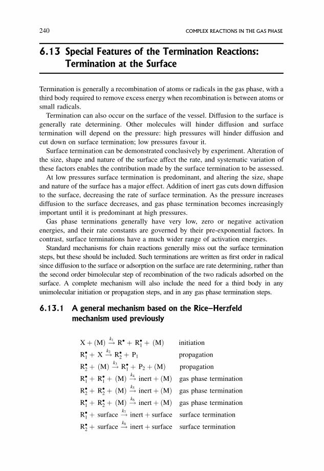
6.13 Special Features of the Termination Reactions:
Termination at the Surface
Termination is generally a recombination of atoms or radicals in the gas phase, with a
third body required to remove excess energy when recombination is between atoms or
small radicals.
Termination can also occur on the surface of the vessel. Diffusion to the surface is
generally rate determining. Other molecules will hinder diffusion and surface
termination will depend on the pressure: high pressures will hinder diffusion and
cut down on surface termination; low pressures favour it.
Surface termination can be demonstrated conclusively by experiment. Alteration of
the size, shape and nature of the surface affect the rate, and systematic variation of
these factors enables the contribution made by the surface termination to be assessed.
At low pressures surface termination is predominant, and altering the size, shape
and nature of the surface has a major effect. Addition of inert gas cuts down diffusion
to the surface, decreasing the rate of surface termination. As the pressure increases
diffusion to the surface decreases, and gas phase termination becomes increasingly
important until it is predominant at high pressures.
Gas phase terminations generally have very low, zero or negative activation
energies, and their rate constants are governed by their pre-exponential factors. In
contrast, surface terminations have a much wider range of activation energies.
Standard mechanisms for chain reactions generally miss out the surface termination
steps, but these should be included. Such terminations are written as first order in radical
since diffusion to the surface or adsorption on the surface are rate determining, rather than
the second order bimolecular step of recombination of the two radicals adsorbed on the
surface. A complete mechanism will also include the need for a third body in any
unimolecular initiation or propagation steps, and in any gas phase termination steps.
6.13.1 A general mechanism based on the Rice–Herzfeld
mechanism used previously
Xþ ðMÞ !k1R� þ R�1 þ ðMÞ initiation
R�1 þ X !k2R�2 þ P1 propagation
R�2 þ ðMÞ !k3
R�1 þ P2 þ ðMÞ propagation
R�1 þ R�1 þ ðMÞ !k4
inertþ ðMÞ gas phase termination
R�2 þ R�2 þ ðMÞ !k5
inertþ ðMÞ gas phase termination
R�1 þ R�2 þ ðMÞ !k6
inertþ ðMÞ gas phase termination
R�1 þ surface !k7inertþ surface surface termination
R�2 þ surface !k8inertþ surface surface termination
240 COMPLEX REACTIONS IN THE GAS PHASE
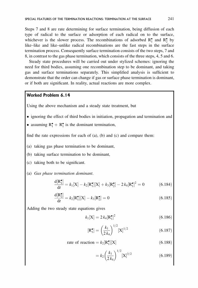
Steps 7 and 8 are rate determining for surface termination, being diffusion of each
type of radical to the surface or adsorption of each radical on to the surface,
whichever is the slower process. The recombinations of adsorbed R�1 and R�2 by
like–like and like–unlike radical recombinations are the fast steps in the surface
termination process. Consequently surface termination consists of the two steps, 7 and
8, in contrast to the gas phase termination, which consists of the three steps, 4, 5 and 6.
Steady state procedures will be carried out under stylized schemes: ignoring the
need for third bodies, assuming one recombination step to be dominant, and taking
gas and surface terminations separately. This simplified analysis is sufficient to
demonstrate that the order can change if gas or surface phase termination is dominant,
or if both are significant. In reality, actual reactions are more complex.
Worked Problem 6.14
Using the above mechanism and a steady state treatment, but
� ignoring the effect of third bodies in initiation, propagation and termination and
� assuming R�1 þ R�1 is the dominant termination,
find the rate expressions for each of (a), (b) and (c) and compare them:
(a) taking gas phase termination to be dominant,
(b) taking surface termination to be dominant,
(c) taking both to be significant.
(a) Gas phase termination dominant.
d½R�1�dt¼ k1½X� k2½R�1�½X� þ k3½R�2� 2 k4½R�1�
2 ¼ 0 ð6:184Þ
d½R�2�dt¼ k2½R�1�½X� k3½R�2� ¼ 0 ð6:185Þ
Adding the two steady state equations gives
k1½X� ¼ 2 k4½R�1�2 ð6:186Þ
½R�1� ¼k1
2 k4
� �1=2
½X�1=2 ð6:187Þ
rate of reaction ¼ k2½R�1�½X� ð6:188Þ
¼ k2
k1
2 k4
� �1=2
½X�3=2 ð6:189Þ
SPECIAL FEATURES OF THE TERMINATION REACTIONS: TERMINATION AT THE SURFACE 241
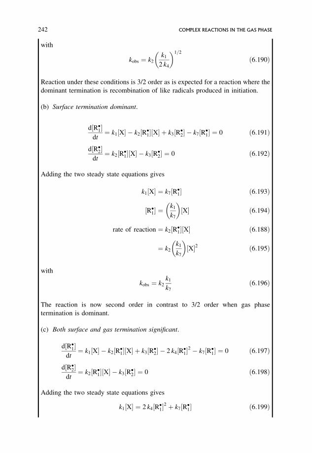
with
kobs ¼ k2
k1
2 k4
� �1=2
ð6:190Þ
Reaction under these conditions is 3/2 order as is expected for a reaction where the
dominant termination is recombination of like radicals produced in initiation.
(b) Surface termination dominant.
d½R�1�dt¼ k1½X� k2½R�1�½X� þ k3½R�2� k7½R�1� ¼ 0 ð6:191Þ
d½R�2�dt¼ k2½R�1�½X� k3½R�2� ¼ 0 ð6:192Þ
Adding the two steady state equations gives
k1½X� ¼ k7½R�1� ð6:193Þ
½R�1� ¼k1
k7
� �½X� ð6:194Þ
rate of reaction ¼ k2½R�1�½X� ð6:188Þ
¼ k2
k1
k7
� �½X�2 ð6:195Þ
with
kobs ¼ k2
k1
k7
ð6:196Þ
The reaction is now second order in contrast to 3/2 order when gas phase
termination is dominant.
(c) Both surface and gas termination significant.
d½R�1�dt¼ k1½X� k2½R�1�½X� þ k3½R�2� 2 k4½R�1�
2 k7½R�1� ¼ 0 ð6:197Þ
d½R�2�dt¼ k2½R�1�½X� k3½R�2� ¼ 0 ð6:198Þ
Adding the two steady state equations gives
k1½X� ¼ 2 k4½R�1�2 þ k7½R�1� ð6:199Þ
242 COMPLEX REACTIONS IN THE GAS PHASE
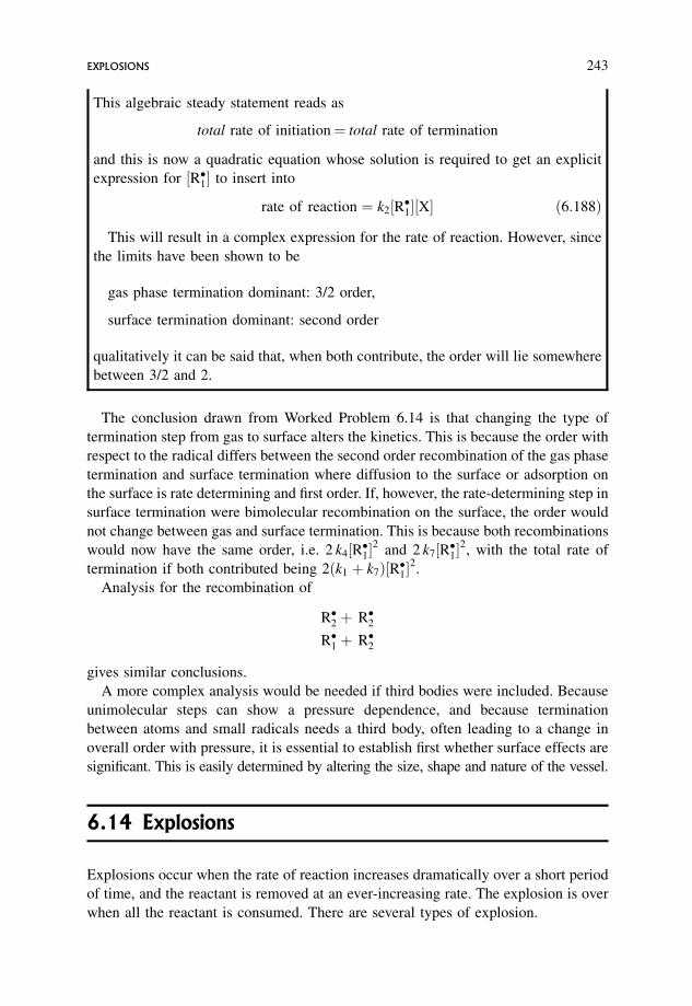
This algebraic steady statement reads as
total rate of initiation¼ total rate of termination
and this is now a quadratic equation whose solution is required to get an explicit
expression for ½R�1� to insert into
rate of reaction ¼ k2½R�1�½X� ð6:188Þ
This will result in a complex expression for the rate of reaction. However, since
the limits have been shown to be
gas phase termination dominant: 3/2 order,
surface termination dominant: second order
qualitatively it can be said that, when both contribute, the order will lie somewhere
between 3/2 and 2.
The conclusion drawn from Worked Problem 6.14 is that changing the type of
termination step from gas to surface alters the kinetics. This is because the order with
respect to the radical differs between the second order recombination of the gas phase
termination and surface termination where diffusion to the surface or adsorption on
the surface is rate determining and first order. If, however, the rate-determining step in
surface termination were bimolecular recombination on the surface, the order would
not change between gas and surface termination. This is because both recombinations
would now have the same order, i.e. 2 k4½R�1�2
and 2 k7½R�1�2, with the total rate of
termination if both contributed being 2ðk1 þ k7Þ½R�1�2.
Analysis for the recombination of
R�2 þ R�2R�1 þ R�2
gives similar conclusions.
A more complex analysis would be needed if third bodies were included. Because
unimolecular steps can show a pressure dependence, and because termination
between atoms and small radicals needs a third body, often leading to a change in
overall order with pressure, it is essential to establish first whether surface effects are
significant. This is easily determined by altering the size, shape and nature of the vessel.
6.14 Explosions
Explosions occur when the rate of reaction increases dramatically over a short period
of time, and the reactant is removed at an ever-increasing rate. The explosion is over
when all the reactant is consumed. There are several types of explosion.
EXPLOSIONS 243
6.14.1 Autocatalysis and autocatalytic explosions
For most straight chains, termination balances initiation, and the radical concentra-
tions remain in the steady state. However, there are some straight chains where the
termination becomes negligible and the radical concentration can build up to large
values well past the steady state region. The reaction becomes autocatalytic as the
reaction rate increases dramatically with the build-up in radical concentration, and if
the increase is very rapid an explosion can occur.
6.14.2 Thermal explosions
Under normal conditions, reactions are carried out at constant temperature where
there is thermal equilibrium between the reaction vessel and thermostat. However, if
the reaction is highly exothermic, the heat liberated cannot be dissipated quickly to
the surroundings, the reaction will self-heat, leading to a rapid increase in rate which,
if great enough, can lead to an explosion.
6.14.3 Branched chain explosions
In straight chain propagation one radical is destroyed while another is produced, so
that the net change in the number of radicals is zero.
In contrast, in a branched chain, as one radical is destroyed more than one radical is
produced, so that there is a net increase in the number of radicals as a result of
propagation.
R�1 þ X! Pþ R�2 straight chain
R�1 þ X! Pþ �R�2 branched chain
For branching to occur � > 1, and can often be 2 or 3, though rarely greater. There
are occasions (see Section 6.15 on degenerate branching) where � is just slightly
greater than unity, and under these circumstances a different situation will occur.
Straight and branched chain propagation can occur simultaneously, or one can
dominate. If a steady state concentration of radicals is set up and maintained
throughout, reaction will occur at a finite rate, and termination will be able to cope
with production of radicals from initiation, and straight and branched chain propaga-
tion. However, when branching occurs it allows the possibility of a continuing build-
up of radicals if termination cannot cope with the branching, and if the build-up is
sufficiently extensive explosions can occur.
Worked Problem 6.15
Question. In a branched chain reaction with � ¼ 2, there is a consequent build-up
of radicals with each cycle of branched chain propagation:
R� þ X! 2 R�
244 COMPLEX REACTIONS IN THE GAS PHASE
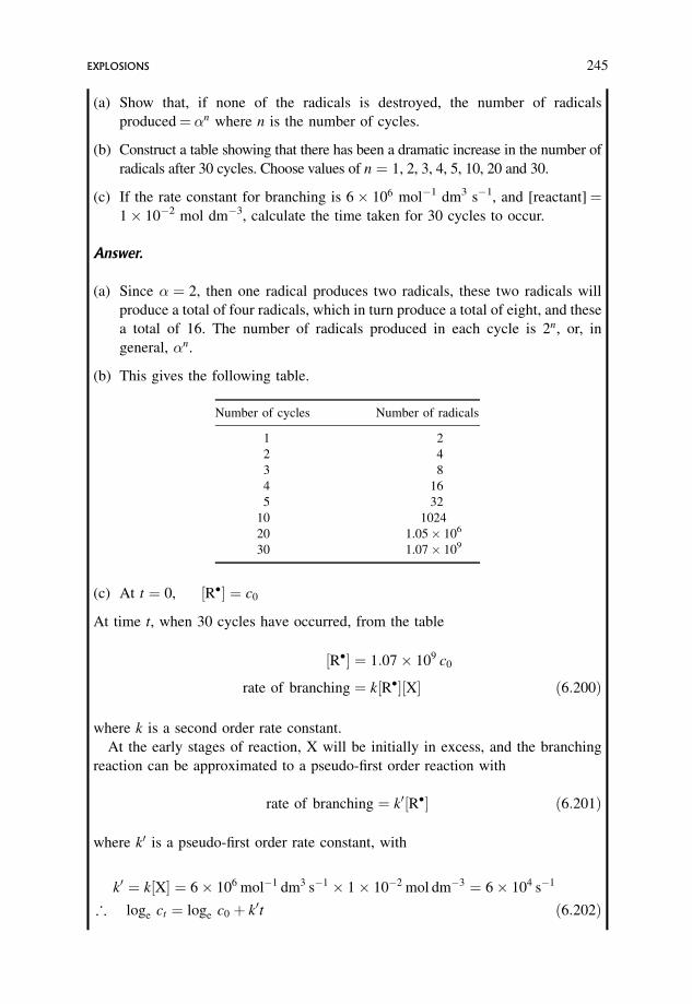
(a) Show that, if none of the radicals is destroyed, the number of radicals
produced¼ �n where n is the number of cycles.
(b) Construct a table showing that there has been a dramatic increase in the number of
radicals after 30 cycles. Choose values of n ¼ 1, 2, 3, 4, 5, 10, 20 and 30.
(c) If the rate constant for branching is 6� 106 mol1 dm3 s1, and [reactant]¼1� 102 mol dm3, calculate the time taken for 30 cycles to occur.
Answer.
(a) Since � ¼ 2, then one radical produces two radicals, these two radicals will
produce a total of four radicals, which in turn produce a total of eight, and these
a total of 16. The number of radicals produced in each cycle is 2n, or, in
general, �n.
(b) This gives the following table.
Number of cycles Number of radicals
1 2
2 4
3 8
4 16
5 32
10 1024
20 1.05� 106
30 1.07� 109
(c) At t ¼ 0, ½R�� ¼ c0
At time t, when 30 cycles have occurred, from the table
½R�� ¼ 1:07� 109 c0
rate of branching ¼ k½R��½X� ð6:200Þ
where k is a second order rate constant.
At the early stages of reaction, X will be initially in excess, and the branching
reaction can be approximated to a pseudo-first order reaction with
rate of branching ¼ k0½R�� ð6:201Þ
where k0 is a pseudo-first order rate constant, with
k0 ¼ k½X� ¼ 6� 106 mol1 dm3 s1 � 1� 102 mol dm3 ¼ 6� 104 s1
; loge ct ¼ loge c0 þ k0t ð6:202Þ
EXPLOSIONS 245
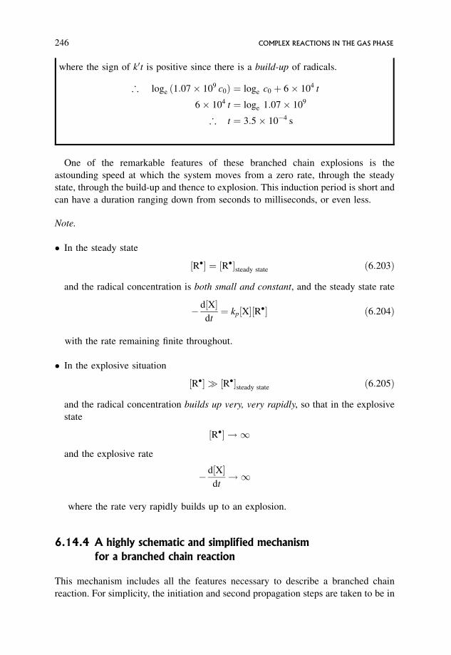
where the sign of k0t is positive since there is a build-up of radicals.
; loge ð1:07� 109 c0Þ ¼ loge c0 þ 6� 104 t
6� 104 t ¼ loge 1:07� 109
; t ¼ 3:5� 104 s
One of the remarkable features of these branched chain explosions is the
astounding speed at which the system moves from a zero rate, through the steady
state, through the build-up and thence to explosion. This induction period is short and
can have a duration ranging down from seconds to milliseconds, or even less.
Note.
� In the steady state
½R�� ¼ ½R��steady state ð6:203Þ
and the radical concentration is both small and constant, and the steady state rate
d½X�dt¼ kp½X�½R�� ð6:204Þ
with the rate remaining finite throughout.
� In the explosive situation
½R�� � ½R��steady state ð6:205Þ
and the radical concentration builds up very, very rapidly, so that in the explosive
state
½R�� ! 1
and the explosive rate
d½X�dt!1
where the rate very rapidly builds up to an explosion.
6.14.4 A highly schematic and simplified mechanism
for a branched chain reaction
This mechanism includes all the features necessary to describe a branched chain
reaction. For simplicity, the initiation and second propagation steps are taken to be in
246 COMPLEX REACTIONS IN THE GAS PHASE
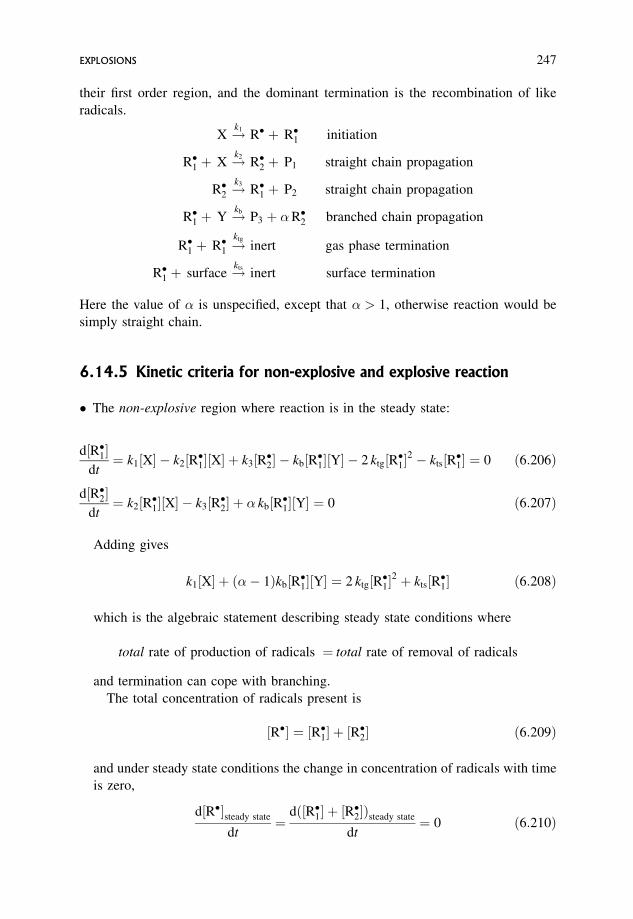
their first order region, and the dominant termination is the recombination of like
radicals.
X !k1R� þ R�1 initiation
R�1 þ X !k2R�2 þ P1 straight chain propagation
R�2 !k3
R�1 þ P2 straight chain propagation
R�1 þ Y !kbP3 þ �R�2 branched chain propagation
R�1 þ R�1 !ktg
inert gas phase termination
R�1 þ surface !ktsinert surface termination
Here the value of � is unspecified, except that � > 1, otherwise reaction would be
simply straight chain.
6.14.5 Kinetic criteria for non-explosive and explosive reaction
� The non-explosive region where reaction is in the steady state:
d½R�1�dt¼ k1½X� k2½R�1�½X� þ k3½R�2� kb½R�1�½Y� 2 ktg½R�1�
2 kts½R�1� ¼ 0 ð6:206Þ
d½R�2�dt¼ k2½R�1�½X� k3½R�2� þ � kb½R�1�½Y� ¼ 0 ð6:207Þ
Adding gives
k1½X� þ ð� 1Þkb½R�1�½Y� ¼ 2 ktg½R�1�2 þ kts½R�1� ð6:208Þ
which is the algebraic statement describing steady state conditions where
total rate of production of radicals ¼ total rate of removal of radicals
and termination can cope with branching.
The total concentration of radicals present is
½R�� ¼ ½R�1� þ ½R�2� ð6:209Þ
and under steady state conditions the change in concentration of radicals with time
is zero,
d½R��steady state
dt¼
dð½R�1� þ ½R�2�Þsteady state
dt¼ 0 ð6:210Þ
EXPLOSIONS 247
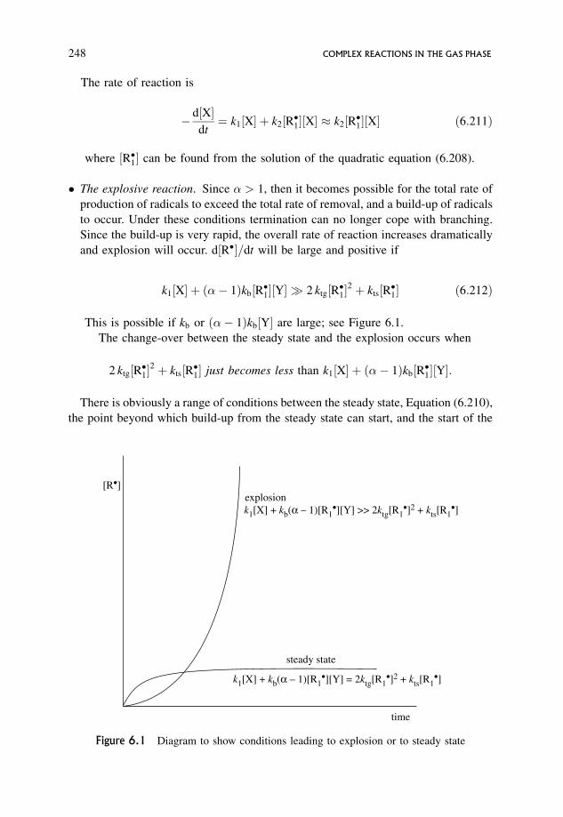
The rate of reaction is
d½X�dt¼ k1½X� þ k2½R�1�½X� � k2½R�1�½X� ð6:211Þ
where ½R�1� can be found from the solution of the quadratic equation (6.208).
� The explosive reaction. Since � > 1, then it becomes possible for the total rate of
production of radicals to exceed the total rate of removal, and a build-up of radicals
to occur. Under these conditions termination can no longer cope with branching.
Since the build-up is very rapid, the overall rate of reaction increases dramatically
and explosion will occur. d½R��=dt will be large and positive if
k1½X� þ ð� 1Þkb½R�1�½Y� � 2 ktg½R�1�2 þ kts½R�1� ð6:212Þ
This is possible if kb or ð� 1Þkb½Y� are large; see Figure 6.1.
The change-over between the steady state and the explosion occurs when
2 ktg½R�1�2 þ kts½R�1� just becomes less than k1½X� þ ð� 1Þkb½R�1�½Y�:
There is obviously a range of conditions between the steady state, Equation (6.210),
the point beyond which build-up from the steady state can start, and the start of the
[R•]
time
steady state
explosionk1[X] + kb(α _ 1)[R1
•][Y] >> 2ktg[R1•]2 + kts[R1
•]
k1[X] + kb(α _ 1)[R1•][Y] = 2ktg[R1
•]2 + kts[R1•]
Figure 6.1 Diagram to show conditions leading to explosion or to steady state
248 COMPLEX REACTIONS IN THE GAS PHASE
explosive stage, Equation (6.212). This generally shows up as a very sharp change in
the character of the reaction, though in fact, it is a progressive though very, very fast
change. As with the build-up to the steady state, build-up from the steady state to the
explosive state can only be studied using very fast techniques.
6.14.6 A typical branched chain reaction showing explosion limits
The reaction between hydrogen and oxygen is a branched chain reaction which shows
explosive regions. It has been very extensively studied, and appears to have a very
complex mechanism.
All mixtures explode above 600 �C, but in the range 450–600 �C there are certain
pressures and temperatures at which reaction is explosive, while at others reaction
occurs at a slow rate. These are related to the relative importance of gas phase and
surface termination just balancing branching.
A simplified mechanism illustrating the essential features of the H2/O2 reaction
2 H2ðgÞ þ O2ðgÞ ! 2 H2OðgÞ
The main radicals present are H�, OH�, O� and HO�2, and the basic mechanism
proposed is
H2 þ O2 ! 2 OH� initiation
OH� þ H2 ! H2Oþ H� straight propagation
H� þ O2 ! OH� þ O� branching propagation
O� þ H2 ! OH� þ O� branching propagation
Mþ H� þ O2 ! HO�2 þ M gas phase termination since
HO�2 is relatively stable; even
though it is a radical
HO�2 þ surface! 1
2H2Oþ 3
4O2 surface termination
H� þ surface! inert species
O� þ surface! inert species
OH� þ surface! inert species
Under certain conditions there is competition between
HO�2 þ surface! 1
2H2Oþ 3
4O2 surface termination
EXPLOSIONS 249
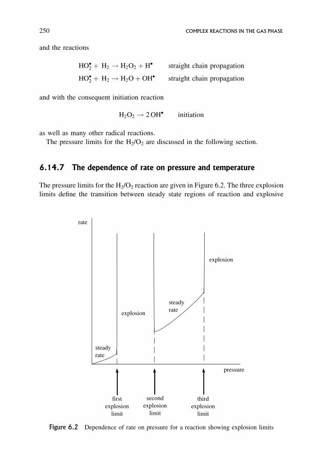
and the reactions
HO�2 þ H2 ! H2O2 þ H� straight chain propagation
HO�2 þ H2 ! H2Oþ OH� straight chain propagation
and with the consequent initiation reaction
H2O2 ! 2 OH� initiation
as well as many other radical reactions.
The pressure limits for the H2/O2 are discussed in the following section.
6.14.7 The dependence of rate on pressure and temperature
The pressure limits for the H2/O2 reaction are given in Figure 6.2. The three explosion
limits define the transition between steady state regions of reaction and explosive
firstexplosion
limit
steadyrate
rate
steadyrateexplosion
explosion
secondexplosion
limit
thirdexplosion
limit
pressure
Figure 6.2 Dependence of rate on pressure for a reaction showing explosion limits
250 COMPLEX REACTIONS IN THE GAS PHASE
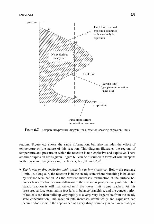
regions. Figure 6.3 shows the same information, but also includes the effect of
temperature on the nature of this reaction. This diagram illustrates the regions of
temperature and pressure in which the reaction is non-explosive and explosive. There
are three explosion limits given. Figure 6.3 can be discussed in terms of what happens
as the pressure changes along the lines a, b, c, d, and a0; d0.
� The lower, or first explosion limit occurring at low pressures. Below the pressure
limit, i.e. along a, b, the reaction is in the steady state where branching is balanced
by surface termination. As the pressure increases, termination at the surface be-
comes less effective because diffusion to the surface is progressively inhibited, but
steady reaction is still maintained until the lower limit is just reached. At this
pressure, surface termination just fails to balance branching, and the concentration
of radicals can then build up very rapidly to a very, very large value from the steady
state concentration. The reaction rate increases dramatically and explosion can
occur. It does so with the appearance of a very sharp boundary, which in actuality is
No explosion:steady rate
Explosion
Second limit gas phase terminationtakes over
b
c
d
Third limit: thermalexplosion combined with autocatalyticexplosion
d′
a′ a
pressure
First limit: surfacetermination takes over
temperature
Figure 6.3 Temperature/pressure diagram for a reaction showing explosion limits
EXPLOSIONS 251
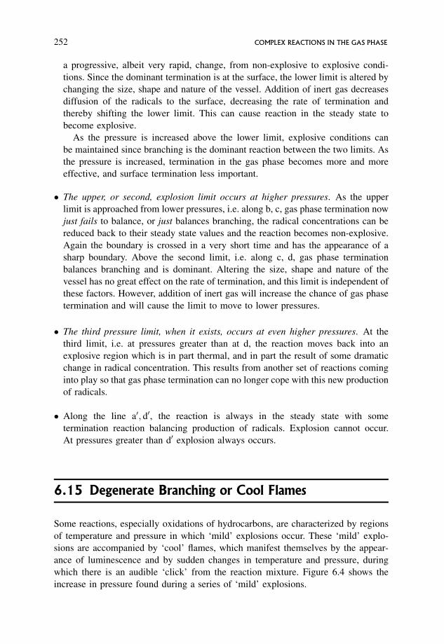
a progressive, albeit very rapid, change, from non-explosive to explosive condi-
tions. Since the dominant termination is at the surface, the lower limit is altered by
changing the size, shape and nature of the vessel. Addition of inert gas decreases
diffusion of the radicals to the surface, decreasing the rate of termination and
thereby shifting the lower limit. This can cause reaction in the steady state to
become explosive.
As the pressure is increased above the lower limit, explosive conditions can
be maintained since branching is the dominant reaction between the two limits. As
the pressure is increased, termination in the gas phase becomes more and more
effective, and surface termination less important.
� The upper, or second, explosion limit occurs at higher pressures. As the upper
limit is approached from lower pressures, i.e. along b, c, gas phase termination now
just fails to balance, or just balances branching, the radical concentrations can be
reduced back to their steady state values and the reaction becomes non-explosive.
Again the boundary is crossed in a very short time and has the appearance of a
sharp boundary. Above the second limit, i.e. along c, d, gas phase termination
balances branching and is dominant. Altering the size, shape and nature of the
vessel has no great effect on the rate of termination, and this limit is independent of
these factors. However, addition of inert gas will increase the chance of gas phase
termination and will cause the limit to move to lower pressures.
� The third pressure limit, when it exists, occurs at even higher pressures. At the
third limit, i.e. at pressures greater than at d, the reaction moves back into an
explosive region which is in part thermal, and in part the result of some dramatic
change in radical concentration. This results from another set of reactions coming
into play so that gas phase termination can no longer cope with this new production
of radicals.
� Along the line a0; d0, the reaction is always in the steady state with some
termination reaction balancing production of radicals. Explosion cannot occur.
At pressures greater than d0 explosion always occurs.
6.15 Degenerate Branching or Cool Flames
Some reactions, especially oxidations of hydrocarbons, are characterized by regions
of temperature and pressure in which ‘mild’ explosions occur. These ‘mild’ explo-
sions are accompanied by ‘cool’ flames, which manifest themselves by the appear-
ance of luminescence and by sudden changes in temperature and pressure, during
which there is an audible ‘click’ from the reaction mixture. Figure 6.4 shows the
increase in pressure found during a series of ‘mild’ explosions.
252 COMPLEX REACTIONS IN THE GAS PHASE
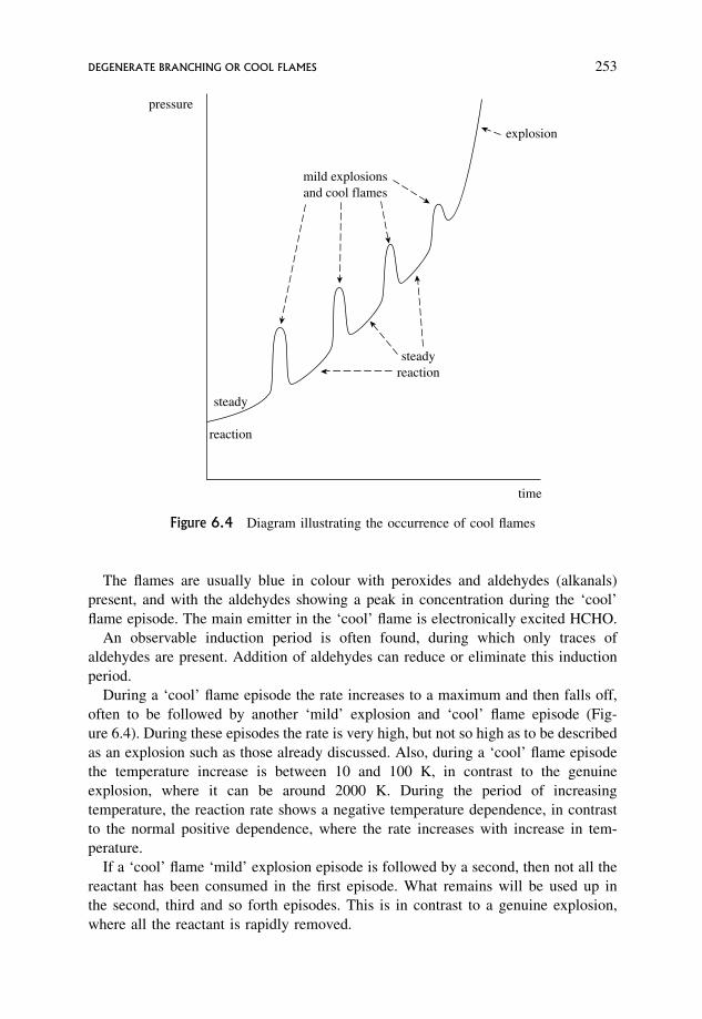
The flames are usually blue in colour with peroxides and aldehydes (alkanals)
present, and with the aldehydes showing a peak in concentration during the ‘cool’
flame episode. The main emitter in the ‘cool’ flame is electronically excited HCHO.
An observable induction period is often found, during which only traces of
aldehydes are present. Addition of aldehydes can reduce or eliminate this induction
period.
During a ‘cool’ flame episode the rate increases to a maximum and then falls off,
often to be followed by another ‘mild’ explosion and ‘cool’ flame episode (Fig-
ure 6.4). During these episodes the rate is very high, but not so high as to be described
as an explosion such as those already discussed. Also, during a ‘cool’ flame episode
the temperature increase is between 10 and 100 K, in contrast to the genuine
explosion, where it can be around 2000 K. During the period of increasing
temperature, the reaction rate shows a negative temperature dependence, in contrast
to the normal positive dependence, where the rate increases with increase in tem-
perature.
If a ‘cool’ flame ‘mild’ explosion episode is followed by a second, then not all the
reactant has been consumed in the first episode. What remains will be used up in
the second, third and so forth episodes. This is in contrast to a genuine explosion,
where all the reactant is rapidly removed.
pressure
mild explosionsand cool flames
explosion
steadyreaction
steady
reaction
time
Figure 6.4 Diagram illustrating the occurrence of cool flames
DEGENERATE BRANCHING OR COOL FLAMES 253
Sometimes, a ‘cool’ flame may be followed by a genuine explosion. Here the ‘cool’
flame behaviour is lost after the first increase in rate, which does not fall off, but
moves straight into the genuine explosion, believed to be thermal in nature.
A series of ‘mild’ explosions is more general at low pressures and low tempera-
tures, in contrast to the high temperatures and pressures at which a ‘mild’ explosion
leads into a genuine explosion. Typical temperature limits for hydrocarbons are
approximately 280–410 �C, with pressure limits around 100–150 mmHg.
‘Cool’ flame behaviour is the result of highly limited degenerate branching, where
the branching coefficient, �, is small, e.g. is of the order of 1.1, compared with being
of the order of two or three in normal branching.
Most of the reaction occurs via straight chain propagation with only a small amount
going via the branching propagation, in contrast to the earlier type of explosion,
where most of the reaction goes via branching propagation.
Since branching is infrequent compared to straight chain propagation, there is only
a very slow build-up of radicals beyond the steady state concentration. Because
branching is so infrequent the build-up to large radical concentrations takes a long
time, of the order of minutes, in contrast to the very rapid build-up into explosion,
such as 103 s, for the normal branching reaction. During this period, termination is
not able to cope with the infrequent branching of the ‘cool’ flame reaction. Each
‘cool’ flame often lasts for a time of the order of seconds.
Hydrocarbon combustions result in many varied products, and these depend on the
temperature, in particular when the temperature is above or below the high
temperature limit for ‘cool’ flame behaviour. At low temperatures, alcohols, alde-
hydes (alkanals) and ketones (alkanones) predominate, whereas at high temperatures
the products are mainly saturated and unsaturated hydrocarbons of lower molecular
weight than the reactant, along with hydrogen peroxide. The organic peroxides
increase in concentration prior to the ‘cool’ flame episode and decrease as the ‘cool’
flame passes, though at this stage the hydrogen peroxide increases. Aldehydes show a
peak in concentration during the ‘cool’ flame.
The effect of temperature is unusual as ‘cool’ flame combustion reactions show a
region of temperatures and pressures in which the rate shows anomalous behaviour:
the rate decreases as the temperature increases – the negative temperature coefficient
effect.
Hydrocarbon combustions are highly complex with very many reactions participat-
ing. Nonetheless, a simplified mechanism can be written containing all the essential
features to explain ‘cool’ flame behaviour.
6.15.1 A schematic mechanism for hydrocarbon combustion
RHþ O2 !k1
R� þ HO�2 initiation
R� þ O2 !k2
RO�2 straight chain propagation
RO�2 !k2
R� þ O2 straight chain propagation (reverse)
254 COMPLEX REACTIONS IN THE GAS PHASE
RO�2 þ RH !k3ROOHþ R� straight chain propagation
ROOH !k4RO� þ OH� degenerate branching
RO� þ RH !k5ROHþ R� propagation
OH� þ RH !k6H2Oþ R� propagation
R� þ R� !ktg
inert gas phase termination
R� þ surface !ktssurface termination
There are other very important reactions which must be considered. With increasing
temperature there is competition between branching resulting from production of
ROOH from RO�2, step 3, and production of alkenes via R�:
R� þ O2 !k2
RO�2 ! branching via ROOH
R� þ O2 ! alkeneþ HO�2
At low temperatures HO�2 is relatively inert and can be ignored, but at high
temperatures it forms hydrogen peroxide by H abstraction from reactant.
HO�2 þ RH! H2O2 þ R�
At even higher temperatures H2O2 can decompose to produce a new branching
sequence:H2O2 ! 2 OH�
RHþ OH� ! R� þ H2O
which has a net overall production of radicals.
Since a wide variety of products are formed in combustion reactions, many more
reactions should be included in the sequence. However, the nine reactions quoted in
the simple mechanism are all that is needed to explain ‘cool’ flame behaviour. This is
discussed in the following worked problem.
Worked Problem 6.16
Question.
(a) In the simplified mechanism, the first two steps of the straight chain propaga-
tion make up a reversible reaction. Write down the possible fates of the RO�2radical, and state what are the overall effects of these fates.
(b) Figure 6.5 gives the essential features of the energetics of this reaction. Work
out the effect of temperature on the rates of the forward and back steps, and on
the position of equilibrium.
DEGENERATE BRANCHING OR COOL FLAMES 255
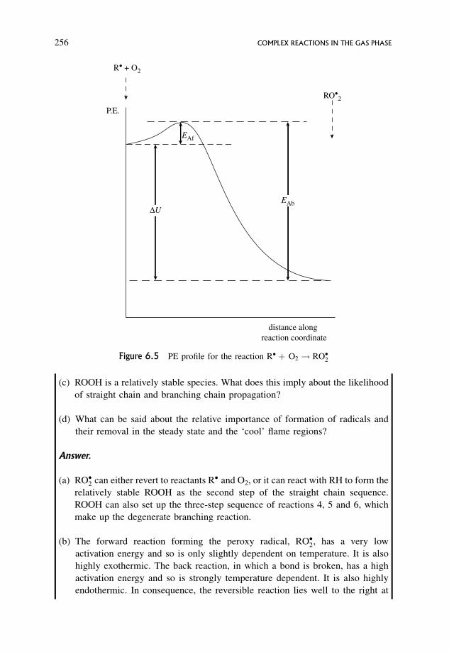
(c) ROOH is a relatively stable species. What does this imply about the likelihood
of straight chain and branching chain propagation?
(d) What can be said about the relative importance of formation of radicals and
their removal in the steady state and the ‘cool’ flame regions?
Answer.
(a) RO�2 can either revert to reactants R� and O2, or it can react with RH to form the
relatively stable ROOH as the second step of the straight chain sequence.
ROOH can also set up the three-step sequence of reactions 4, 5 and 6, which
make up the degenerate branching reaction.
(b) The forward reaction forming the peroxy radical, RO�2, has a very low
activation energy and so is only slightly dependent on temperature. It is also
highly exothermic. The back reaction, in which a bond is broken, has a high
activation energy and so is strongly temperature dependent. It is also highly
endothermic. In consequence, the reversible reaction lies well to the right at
RO•2
R• + O2
P.E.
distance along reaction coordinate
∆UEAb
EAf
Figure 6.5 PE profile for the reaction R� þ O2 ! RO�2
256 COMPLEX REACTIONS IN THE GAS PHASE
low temperatures, favouring RO�2 and its subsequent reaction. On the other
hand, high temperatures will favour the back reaction leading to the breakdown
of the RO�2 back to R� and O2, decreasing the chances of ROOH being formed.
Hence alternate increases and decreases of temperature can cause this
equilibrium to oscillate.
(c) Since ROOH is relatively inert, very many cycles of the straight chain
propagation sequence can occur before ROOH forms RO� and OH�, the net
effect of which is that two radicals produce four. However, this branching is
relatively infrequent compared with straight chain propagation, which dom-
inates, and this gives an overall � of close to unity. This places these
combustion reactions in the class of degenerate branching in contrast to
explosive reactions such as H2/O2 where most of the reaction goes via
branching.
(d) In the steady state
total rate of production of radicals via ¼ total rate of removal of radicals via
initiation and branching propagation gas phase and surface termination
In the ‘cool’ flame episode the total rate of termination can no longer cope with the
branching, the production of radicals increases and reaction moves into a ‘cool’
flame episode.
6.15.2 Chemical interpretation of ‘cool’ flame behaviour
When there are several episodes of ‘cool’ flames the reaction is oscillatory. The
crucial feature is the reversible reaction
R� þ O2!
k2
k2
RO�2
At low temperatures, reaction lies well to the right favouring RO�2, increasing the
chance of ROOH being formed, leading to the branching reaction which increases the
rate of oxidation. These subsequent reactions, 4, 5 and 6, are highly exothermic and
lead to an increase in temperature due to self-heating.
As the temperature rises, the reversible reaction moves increasingly to the left
favouring R� over RO�2. This increases the chance of termination rather than
branching, leading to a decrease in the overall rate, and a decrease in the heat
released by the reaction. The exothermic reactions 5 and 6 become less likely and
self-heating decreases. This whole process occurs in a matter of seconds. The
aldehydes, and particularly the emitting HCHO, build up during the period of
increasing temperature and fade away during the period of decreasing temperature.
Hence luminescence builds up and dies away during a ‘cool’ flame episode. If not all
DEGENERATE BRANCHING OR COOL FLAMES 257
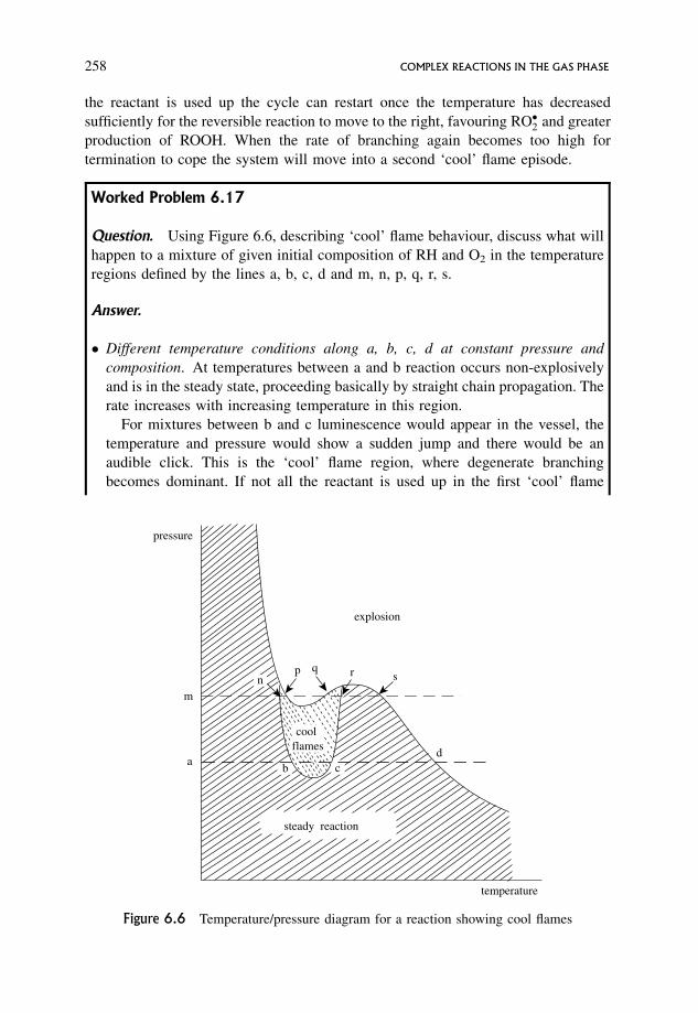
the reactant is used up the cycle can restart once the temperature has decreased
sufficiently for the reversible reaction to move to the right, favouring RO�2 and greater
production of ROOH. When the rate of branching again becomes too high for
termination to cope the system will move into a second ‘cool’ flame episode.
Worked Problem 6.17
Question. Using Figure 6.6, describing ‘cool’ flame behaviour, discuss what will
happen to a mixture of given initial composition of RH and O2 in the temperature
regions defined by the lines a, b, c, d and m, n, p, q, r, s.
Answer.
� Different temperature conditions along a, b, c, d at constant pressure and
composition. At temperatures between a and b reaction occurs non-explosively
and is in the steady state, proceeding basically by straight chain propagation. The
rate increases with increasing temperature in this region.
For mixtures between b and c luminescence would appear in the vessel, the
temperature and pressure would show a sudden jump and there would be an
audible click. This is the ‘cool’ flame region, where degenerate branching
becomes dominant. If not all the reactant is used up in the first ‘cool’ flame
steady reaction
temperature
pressure
explosion
m
ab
n
cd
p qsr
cool flames
Figure 6.6 Temperature/pressure diagram for a reaction showing cool flames
258 COMPLEX REACTIONS IN THE GAS PHASE
episode there will be a succession of ‘cool’ flames. When the overall rate is
studied, the rate increases with temperature as conditions are altered along b, c,
but there comes a stage at which it must start to decrease with increase in
temperature to enable the rate to decrease to the steady state rate which occurs at
temperatures greater than c. This is the anomalous negative temperature coefficient
region. For temperatures between c and d reaction is back to the steady state. At
temperatures somewhat beyond c the rate increases with temperature. At temperatures
greater than d reaction moves into a genuine explosion, thought to be partly thermal
and partly due to other reactions becoming important; see Section 6.15.1.
� Different temperatures along m, n, p, q, r, s for constant pressure and
composition. Between m and n reaction is in the steady state similar to along
a, b. At temperatures between n and p the ‘cool’ flame region is reached with its
accompanying characteristic features. Here the rate increases with increasing
initial temperatures since, at temperatures greater than p but below q, explosion
can occur. However, because the pressure is higher than along a, b, c, d, the
sudden increase in pressure due to a ‘cool’ flame is sufficient to take the reaction
into explosion. Degenerate branching is important in the ‘cool’ flame region, but
thermal explosion can easily take over.
When the initial temperature lies between p and q all mixtures will explode.
For initial temperatures between q and r a ‘cool’ flame region exists, but, in
contrast to region n, p, the overall rate must decrease with increasing tempera-
tures since at r reaction enters the steady state region. Between q and r reaction
has a negative temperature coefficient.
For initial temperatures between r and s reaction is again in the steady state
with straight chain propagation dominant, but for temperatures greater than s
explosion occurs.
Further reading
Laidler K.J., Chemical Kinetics, 3rd edn, Harper and Row, New York, 1987.
Laidler K.J. and Meiser J.H., Physical Chemistry, 3rd edn, Houghton Mifflin, New
York, 1999.
Alberty R.A. and Silbey R.J., Physical Chemistry, 2nd edn, Wiley, New York, 1996.
Logan S.R., Fundamentals of Chemical Kinetics, Addison Wesley, Reading, MA,
1996.
*Nicholas J., Chemical Kinetics, Harper and Row, New York, 1976.
*Wilkinson F., Chemical Kinetics and Reaction Mechanisms, Van Nostrand Reinhold,
New York, 1980.
Robson Wright M., Fundamental Chemical Kinetics, Horwood, Chichester, 1999.
*Out of print, but should be in university libraries.
FURTHER READING 259
Further problems
1. The bromination of propane C3H8 proceeds via a free radical chain reaction. The
dominant major product is HBr, with 2-bromopropane produced in substantial
amounts. 1-bromopropane, though produced in much smaller amounts, can still be
classified as a major product. 2:3-dimethylbutane is a minor product, and hexane
and 2-methylpentane are trace products.
Deduce a mechanism that will account for these facts.
2. The decomposition of propanal, CH3CH2CHO, is a free radical chain process. The
major products are C2H6 and CO. There are three minor products, butane, pentan-
3-one and hexan-3:4-dione. Of these pentan-3-one is the most abundant. Pentanal
is produced in trace amounts while H2 is found as a very minor trace product. The
reaction is found to be first order at high pressures moving to second order at low
pressures. Deduce a mechanism to fit these facts.
What methods could be used for the detection of the products and intermediates?
3. Using the steady state treatment deduce the rate expressions for the following
mechanisms:
(a) C2H4I2 !k1
C2H4I� þ I�
I� þ C2H4I2 !k2
I2 þ C2H4I�
C2H4I� !k3C2H4 þ I�
I� þ I� þ M !k4I2 þM
(b) C4H9I !k1C4H�9 þ I�
C4H�9 þ C4H9I !k2C4H10 þ C4H8I�
C4H8I� !k3C4H8 þ I�
I� þ C4H9I !k4C4H�9 þ I2
2 I� þ M !k5I2 þM
4. The pyrolysis of propanone is a chain reaction with possible mechanism
CH3COCH3 !k1
CH3CO� þ CH�3
CH3CO� !k2CH�3 þ CO
CH�3 þ CH3COCH3 !k3
CH4 þ�CH2COCH3
�CH2COCH3 !k4
CH�3 þ CH2CO
CH�3 þ�CH2COCH3 !k5
CH3CH2COCH3
260 COMPLEX REACTIONS IN THE GAS PHASE
Using this mechanism explain what is meant by the terms initiation, propagation
and termination, and identify the major and minor products. Find the order of the
reaction and an expression for the observed rate constant.If step 5 is replaced by
CH�3 þ CH�3 !k6
C2H6
predict what the order would become.
Likewise, predict the order if the major termination step became
�CH2COCH3 þ�CH2COCH3 !k7
CH3COCH2CH2COCH3
5. The following is a possible mechanism for the decomposition of propane:
C3H8 !k1
CH�3 þ C2H�5
CH�3 þ C3H8 !k2
CH4 þ C3H�7
C2H�5 þ C3H8 !k3
C2H6 þ C3H�7
C3H�7 !k4
C2H4 þ CH�3
C3H�7 þ C3H�7 !k5
C3H8 þ C3H6
C3H�7 þ C3H�7 !k6
C6H14
Deduce the rate expression for this reaction, and obtain an expression for the
observed rate constant.
6. The following is a schematic mechanism for the bromination of an organic
compound RH:
Br2 þM !k12 Br� þ M
Br� þ RH !k2R� þ HBr
R� þ Br2 !k3
RBrþ Br�
2 Br� þ M !k4Br2 þM
Derive the steady state rate for the production of HBr for this mechanism.
If the inhibition step
R� þ HBr !k2Br� þ RH
were included how would this affect the steady state rate expression?
Derive this rate expression.
FURTHER PROBLEMS 261
7. The following is a possible simplified mechanism for the reaction of chlorine with
ethene C2H4.
Cl2 þM !k12 Cl� þ M
Cl� þ C2H4 !k2
C2H4Cl�
C2H4Cl� þ Cl2 !k3
C2H4Cl2 þ Cl�
Cl� þ Cl� þ M !k1Cl2 þM
C2H4Cl� þ C2H4Cl� !k4C4H8Cl2
Cl� þ C2H4Cl� !k5C2H4Cl2
Why does M appear in steps 1 and 1 and not in steps 4 and 5?
Would a third body be expected to be required for the following termination
reactions?
OH� þ H� ! H2O
CH�3 þ CH�3 ! C2H6
H� þ I� ! HI
CH�3 þ ðCH3Þ3C� ! ðCH3Þ3CCH3
Discuss the effect of temperature and pressure on your conclusion.
8. The following is a problem which combines knowledge about photochemical
reactions and chain reactions.
In a photochemical reaction of overall stoichiometry
Cl2ðgÞ þ cyclo-C6F10ðgÞ ! C6F10Cl2ðgÞ
there was a quantum yield greater than 100. The rate was proportional to [Cl2] and
to the square root of Iabs, but was independent of [C6F10]. No product other than
C6F10Cl2 could be detected. Devise a mechanism which fits the facts.
262 COMPLEX REACTIONS IN THE GAS PHASE
7 Reactions in Solution
Reaction is fundamentally the same in solution and in the gas phase, in so far as both
involve a series of changing configurations of all species involved in the reaction step.
But for solution reactions, these configurations are influenced by the solvent; and
reactant/solvent and solvent/solvent interactions must be considered, with the solvent
becoming an integral part of reaction and the reaction entity.
Aims
By the end of this chapter you should be able to
� know the ways in which the solvent can affect reactions in solution
� appreciate the differences between reactions in the gas phase and solution
� understand the ways in which charges or dipoles in the reactants can affect therate and the rate constant
� adapt transition state theory from gas phase to solution
� discuss the primary salt effect and make corrections for non-ideality
� discuss the effect of the solvent on the rate constant in terms of charges of thereactants and the relative permittivity of the solvent and
� follow an outline of the effect of charge, solvent, reactant complexity and changein solvation pattern on the reaction rate.
7.1 The Solvent and its Effect on Reactions in Solution
There are three properties that are important here: the permittivity of the solvent, the
viscosity of the solvent and the polarizability of the molecules of the solvent.
An Introduction to Chemical Kinetics. Margaret Robson Wright# 2004 John Wiley & Sons, Ltd. ISBNs: 0-470-09058-8 (hbk) 0-470-09059-6 (pbk)
The solvent is the medium, or dielectric, which modifies the electrostatic interac-
tions between charges. It reduces the field strength due to the charges, it reduces the
forces acting on the charges and it reduces the potential energy of interaction between
the charges. The factor by which it reduces these quantities is the relative permittivity, "r.
The larger the value of "r, the smaller will be the forces of interaction between the charges.
The viscosity, �, of a solvent restricts movement through it. The higher the
viscosity, the slower will particles move around.
The polarizability, �, is a measure of the extent to which the electronic distribution
over a molecule can be distorted by the electric field of charged particles, or dipolar
molecules.
The solvent influences reaction in several ways.
� It can affect the mechanism;
� it can affect the magnitude of the rate constant through the relative permittivity,
viscosity and polarizability and other electronic properties of the solvent;
� it can affect the species involved;
� it can affect any ion pairing, complexing, hydrogen bonding and other association
phenomena.
Differences also arise.
� In contrast to gas phase reactions, reactions involving ions, polar molecules and
charged transition states occur readily in solution.
� Typical molecular and free radical reactions of the gas phase also occur in
solution, but are much less frequent, in contrast to the predominance of this type
of reaction in the gas phase.
� In the gas phase, intermediates are often found in steady state concentrations. In
solution, many of the intermediates are at equilibrium concentrations.
� Steady state concentrations in the gas phase cannot be studied independently of reaction,
but equilibrium concentrations in the solution phase can be found readily. This can
make the kinetic analysis for solution reactions easier than for the gas phase.
� The solvent often has a profound effect on the interpretation of rate constants, EA
or �H 6¼�, A or �S6¼� and �V 6¼�.
� Gas phase reactions have predominantly molecular-type structures for the acti-
vated complex, whereas solution reactions often have predominantly charged or
charge-separated structures.
264 REACTIONS IN SOLUTION
� The effect of the solvent on the activated complex is often crucial:
(a) the permittivity dictates the structure and the charge distribution in the
activated complex;
(b) the change in the structure of the solvent on forming the activated complex
must be explicitly considered;
(c) the shape and size of the activated complex is often to a large extent dictated
by the solvent.
� In both phases, reactants must first diffuse together. In the gas phase the rate of
diffusion is so fast that it has no effect on the rate of reaction. In solution, either
diffusion or reaction can be rate determining. Normally reaction is the slower
process, but in some reactions, such as very fast ionic reactions, diffusion can be
rate determining.
� Molecules in a gas move in straight lines between collisions, but in solution
Brownian motion occurs, with molecules following vastly more irregular paths.
This can have an effect on some reactions.
� Theoretical calculations are less fundamental and rigorous for solution reactions.
This is a consequence of the difficulty of calculating partition functions in
solution. The main focus for solution reactions has been on the thermodynamic
formulation of transition state theory.
7.2 Collision Theory for Reactions in Solution
Gas phase collision formulae (Section 4.1.2) can be used for many reactions in
solution, i.e. for those involving uncharged species forming activated complexes with
little or no charge separation. The theory of such reactions will not be considered
further, and it will be assumed that the gas phase treatment is adequate.
However, modifications are required for reactions involving ions and charged or
charge-separated activated complexes (Problem 4.5(ii) and Tables 7.1 to 7.3).
Experimental results show that
� reactions between like-charged ions have A factors considerably below the gas
phase ZAB, a consequence of repulsive forces between the ions giving a decreased
rate of collision;
� reactions between unlike-charged ions have A factors considerably above ZAB, a
result of attractive forces between the ions increasing the collision rate;
� rate constants depend on the relative permittivity of the solvent.
COLLISION THEORY FOR REACTIONS IN SOLUTION 265
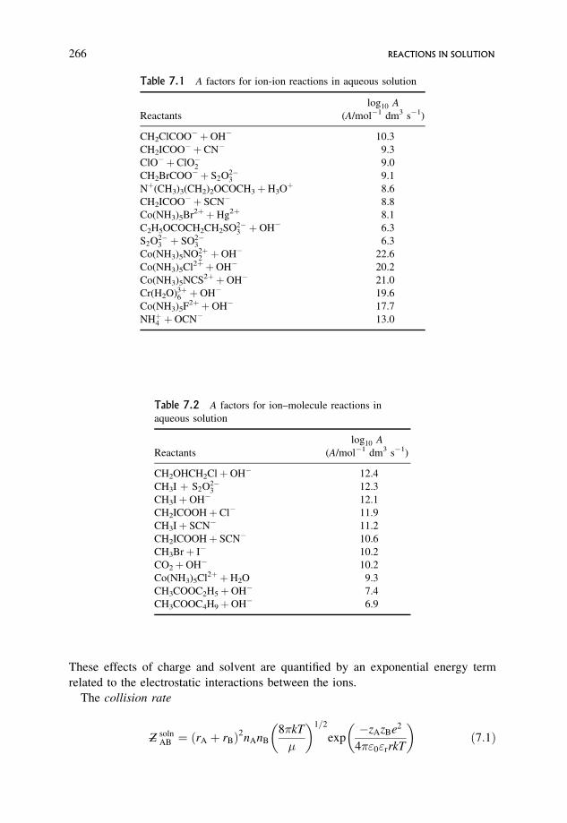
These effects of charge and solvent are quantified by an exponential energy term
related to the electrostatic interactions between the ions.
The collision rate
Z� solnAB ¼ ðrA þ rBÞ2nAnB
8�kT
�
� �1=2
exp�zAzBe2
4�"0"rrkT
� �ð7:1Þ
Table 7.1 A factors for ion-ion reactions in aqueous solution
log10 A
Reactants (A/mol�1 dm3 s�1)
CH2ClCOO� þOH� 10.3
CH2ICOO� þ CN� 9.3
ClO� þ ClO�2 9.0
CH2BrCOO� þ S2O2�3 9.1
Nþ(CH3)3(CH2)2OCOCH3þH3Oþ 8.6
CH2ICOO� þ SCN� 8.8
Co(NH3)5Br2þ þHg2þ 8.1
C2H5OCOCH2CH2SO2�3 þOH� 6.3
S2O2�3 þ SO2�
3 6.3
Co(NH3)5NO2þ2 þOH� 22.6
Co(NH3)5Cl2þ þOH� 20.2
Co(NH3)5NCS2þ þOH� 21.0
Cr(H2O)3þ6 þOH� 19.6
Co(NH3)5F2þ þOH� 17.7
NHþ4 þOCN� 13.0
Table 7.2 A factors for ion–molecule reactions in
aqueous solution
log10 A
Reactants (A/mol�1 dm3 s�1)
CH2OHCH2ClþOH� 12.4
CH3I þ S2O2�3 12.3
CH3IþOH� 12.1
CH2ICOOHþ Cl� 11.9
CH3Iþ SCN� 11.2
CH2ICOOHþ SCN� 10.6
CH3Brþ I� 10.2
CO2þOH� 10.2
Co(NH3)5Cl2þ þH2O 9.3
CH3COOC2H5þOH� 7.4
CH3COOC4H9þOH� 6.9
266 REACTIONS IN SOLUTION
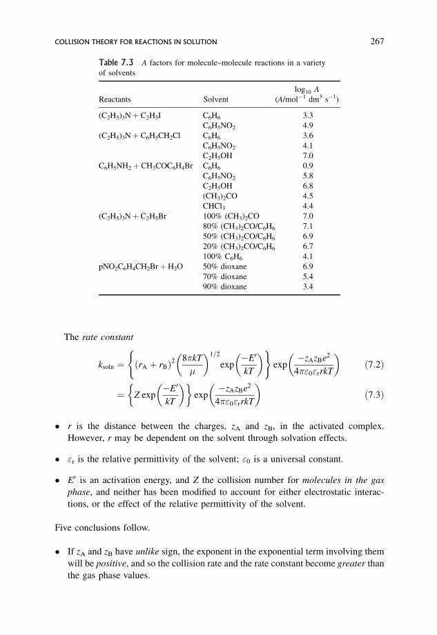
The rate constant
ksoln ¼ ðrA þ rBÞ28�kT
�
� �1=2
exp�E0
kT
� �( )exp
�zAzBe2
4�"0"rrkT
� �ð7:2Þ
¼ Z exp�E0
kT
� �� �exp
�zAzBe2
4�"0"rrkT
� �ð7:3Þ
� r is the distance between the charges, zA and zB, in the activated complex.
However, r may be dependent on the solvent through solvation effects.
� "r is the relative permittivity of the solvent; "0 is a universal constant.
� E0 is an activation energy, and Z the collision number for molecules in the gas
phase, and neither has been modified to account for either electrostatic interac-
tions, or the effect of the relative permittivity of the solvent.
Five conclusions follow.
� If zA and zB have unlike sign, the exponent in the exponential term involving them
will be positive, and so the collision rate and the rate constant become greater than
the gas phase values.
Table 7.3 A factors for molecule–molecule reactions in a variety
of solvents
log10 A
Reactants Solvent (A/mol�1 dm3 s�1)
(C2H5)3Nþ C2H5I C6H6 3.3
C6H5NO2 4.9
(C2H5)3Nþ C6H5CH2Cl C6H6 3.6
C6H5NO2 4.1
C2H5OH 7.0
C6H5NH2þ CH3COC6H4Br C6H6 0.9
C6H5NO2 5.8
C2H5OH 6.8
(CH3)2CO 4.5
CHCl3 4.4
(C2H5)3Nþ C2H5Br 100% (CH3)2CO 7.0
80% (CH3)2CO/C6H6 7.1
50% (CH3)2CO/C6H6 6.9
20% (CH3)2CO/C6H6 6.7
100% C6H6 4.1
pNO2C6H4CH2BrþH2O 50% dioxane 6.9
70% dioxane 5.4
90% dioxane 3.4
COLLISION THEORY FOR REACTIONS IN SOLUTION 267
� If zA and zB have like sign, the exponent in the exponential is negative, and the
solution phase quantities become less than the gas phase values.
� The effect of temperature on the collision rate is complex. In the gas phase the
collision rate is proportional to T1/2, but for solution this is modified by the
exponential term in 1/("rT). Since "r depends on T, it is not immediately clear how
the exponential term modifies the T1/2 term.
� Likewise, the effect of temperature on the solution rate constant is complex.
� The term exp �zAzB e2=4�"0"rrkTð Þ modifies both the gas phase collision rate and
the gas phase activation energy in a complex manner. Equation (7.3) cannot be
written in a simple manner as
ksoln ¼ ða collision number)
(exponential term in the observed activation energy),
in contrast to the simple gas phase expression which can:
k ¼ Z expð�EA=RTÞ: ð7:4Þ
For this reason, transition state theory (see Section 7.3) is a more direct and
straightforward way to give a theoretical discussion of the effect of charge and
solvent on rates.
7.2.1 The concepts of ideality and non-ideality
Because ionic interactions are significant in electrolyte solutions, reactions involving
charges will occur under grossly non-ideal conditions. When the concentration of the
solute in a solution tends to zero, i.e. c! 0, the solution is regarded as ideal.
Interactions present are solvent–solvent, solute–solvent and solute–solute, with only
the solvent–solvent interactions being significant. The non-ideal solution corresponds
to all finite concentrations of solute, other than infinite dilution, which describes the
ideal solution. Non-ideality corresponds physically to all interactions that are over
and above those present in the ideal solution. When the concentration of solute
increases, solute–solute and solute–solvent interactions increase, and these cause
modified solvent–solvent interactions, and all cause increasing non-ideality.
The major factor giving rise to increasing non-ideality, as the solute concentration
increases, is the solute–solute interactions, and these are particularly important when
charges are involved. However, the solute–solvent interactions, i.e. solvation, or the
modified solvent–solvent interactions, must not be forgotten.
Non-ideality is usually handled by the Debye–Huckel theory, and this can be easily
done using transition state theory.
268 REACTIONS IN SOLUTION
7.3 Transition State Theory for Reactions in Solution
The effect of the solvent on the rate constant is considered in terms of non-ideality,
charge on reactants, relative permittivity and change in solvation pattern of the
solvent. Because of the difficulty of assessing partition functions in solution, the
thermodynamic formulation is used. A simplified version is given here.
The basic equation of transition state theory in this form is
k ¼ �kT
h
� �K 6¼ � ð4:39Þ
where K 6¼ � is a concentration equilibrium constant, with one term struck out,
describing the formation of the activated complex (Sections 4.3.3, 4.3.4 and 4.4).
Aþ B ! � ðABÞ6¼ ! products
and
K 6¼ ¼ ½AB�6¼
½A�½B�
!equil
ð7:5Þ
is closely related to K 6¼ �.Remember the meanings of all the various k, � and K 6¼ � in Equation (4.39).
� The k on the left-hand side of the equation is the theoretical rate constant.
� The k in the term �kT=hð Þ is the Boltzmann constant, and the � is the transmission
coefficient, generally taken to be unity.
� K 6¼ � is the equilibrium constant describing the formation of the activated complex
but with one term corresponding to the free translation struck out.
7.3.1 Effect of non-ideality: the primary salt effect
Since K 6¼ � is a concentration equilibrium constant, it is a non-ideal equilibrium
constant, and so k is also a non-ideal rate constant, which incorporates all the factors
causing non-ideality. Since these factors will be different for different reactions, these
rate constants and their derived kinetic parameters should not be used for compar-
isons of reactions, but must first be converted to ones where the effects of non-ideality
have been taken care of, i.e. ideal values.
The Debye–Huckel theory gives a way of dealing with non-ideality in solutions of
electrolytes. The ideal free energy can be calculated, and the difference between the
TRANSITION STATE THEORY FOR REACTIONS IN SOLUTION 269
actual free energy and this ideal value gives the non-ideal contribution resulting from
all the ionic interactions. This difference, in turn, is considered to manifest itself as an
activity coefficient, i, for solute i, and is defined by
ai ¼ i ci ð7:6Þ
where ai is the activity, and i ! 1 when ci ! 0, i.e. in the ideal solution.
Under non-ideal conditions
�i ¼ �i þ RT loge i ci ð7:7Þ
where �i, the chemical potential, refers to the solute species i.
The Debye–Huckel limiting law equation gives an expression for the activity
coefficient of an ion as
log10 i ¼ �A z2i
ffiffiIp
ð7:8Þ
where A ¼ 0:510 mol�1/2 dm3/2 for water at 25 �C, zi is the charge on the ion and I is
the ionic strength defined as
I ¼ 1
2
Xi
ðci z2i Þ ð7:9Þ
where this sum is over all charged species in the solution.
The ideal equilibrium constant for the formation of the activated complex is given
in terms of activities:
K6¼ideal ¼
aAB 6¼
aA aB
� �ð7:10Þ
This ideal equilibrium constant can also be written as
K6¼ideal ¼
aAB6¼
aA aB
� �¼ ½AB�6¼
½A�½B�
!AB 6¼
AB
� �ð7:11Þ
¼ K6¼non-ideal
AB 6¼
AB
� �ð7:12Þ
;K6¼non-ideal ¼ K
6¼ideal
AB
AB 6¼
� �ð7:13Þ
Each of K6¼ideal and K
6¼non-ideal can be written as the product of the corresponding K 6¼ �
and the factor relating to the internal translation in the activated complex. Since this
factor appears on both sides of the equation it will cancel out, and so Equation (7.13)
becomes
K6¼�non-ideal ¼ K
6¼�ideal
AB
AB 6¼
� �ð7:14Þ
270 REACTIONS IN SOLUTION
Since both k and K 6¼ � appearing in Equation (4.39) are concentration constants, and
not constants in terms of activities,
k ¼ �kT
hK 6¼ � ð4:39Þ
this equation can be rewritten in terms of a knon-ideal and a K6¼�non-ideal:
knon-ideal ¼�kT
hK6¼�non-ideal ð7:15Þ
which with Equation (7.14) gives
knon-ideal ¼�kT
hK6¼ �ideal
AB
AB 6¼ð7:16Þ
¼ kideal
AB
AB 6¼ð7:17Þ
Note: the quotient of activity coefficients in the equation for the rate constant, i.e.
Equation (7.17), is the reciprocal of the quotient of activity coefficients appearing in
equations for the ideal equilibrium constants, Equations (7.11) and (7.12). This is
because Equation (7.17) is in terms of the non-ideal rate constant.
Remember: observed experimental quantities inevitably are non-ideal quantities.
If all the activity coefficients are unity, the solution corresponds to ideality.
However, for reactions in solution this is unlikely to happen, especially if there are
ions or charge-separated species involved.
Remember: K6¼�non-ideal is fundamentally a partition function quantity, and in the
above treatment this has been converted to one involving activity coefficients.
In transition state theory the calculated rate constant is given by
k ¼ �kT
h
Q6¼�
QAQB
exp�E0
RT
� �ð4:20Þ
For gases, QA and QB are readily found from spectroscopic data, but Q 6¼ � for the
activated complex can only be calculated if the potential energy surface is accurately
known in the region of the critical configuration. It cannot be measured experimen-
tally – the activated complex is merely a special critical configuration.
Likewise, AB 6¼ also cannot be measured experimentally, although, like QA and QB,
A and B can be measured, and at first sight the conversion given above may seem to
give little improvement. However, for ion–ion and ion–molecule reactions, the
Debye–Huckel theory, see Equation (7.8), can calculate the activity coefficient for
any charged species and convert Equation (7.17) into a useful form. For other
reactions the approach is only qualitative, but for them the effects of non-ideality are
much smaller.
Taking logarithms to base 10 Equation (7.17) gives
log10 knon-ideal ¼ log10 kideal þ log10 A þ log10 B � log10 AB6¼ ð7:18Þ
Note: logarithms are to base 10 because the Debye–Huckel equation is given in
logarithms to base 10.
TRANSITION STATE THEORY FOR REACTIONS IN SOLUTION 271
The Debye–Huckel equation for very dilute solutions can be used for each activity
coefficient:
log10 i ¼ �A z2i
ffiffiIp
ð7:8Þ
where A is the Debye–Huckel constant, which is dependent on temperature and takes
the value 0.510 mol�1/2 dm3/2 for water at 25 �C.
The activated complex has charge zA þ zB. Taking Equations (7.18) and (7.8)
together gives
log10 knon-ideal ¼ log10 kideal � A z2A
ffiffiIp� A z2
B
ffiffiIpþ AðzA þ zBÞ2
ffiffiIp
ð7:19Þ¼ log10 kideal � A z2
A
ffiffiIp� A z2
B
ffiffiIpþ A z2
A
ffiffiIpþ A z2
B
ffiffiIpþ 2 A zA zB
ffiffiIp
ð7:20Þlog10 knon-ideal ¼ log10 kideal þ 2 A zA zB
ffiffiIp
ð7:21Þ
The treatment can be extended to higher ionic strengths, giving
log10 knon-ideal ¼ log10 kideal þ 2 A zA zB
ffiffiIp
1þffiffiIp ð7:22Þ
This is called the primary salt effect.
Reactions involving charged reactants will occur under non-ideal conditions, and
will show a dependence on ionic strength (Equations (7.21) and (7.22). This means
that it is necessary to be able to work out the ionic strength from the experimental
conditions. The following problem gives practice with this.
Worked Problem 7.1
Question. The reaction
Fe2þðaqÞ þ ½CoðC2O4Þ3�3�ðaqÞ ! Fe3þðaqÞ þ 3 C2O2�
4 ðaqÞ þ Co2þðaqÞ
can be carried out at various ionic strengths, either without added salts, or with
them. The Fe2þ is introduced as Fe(NO3)2, and the Co(C2O4)3�3 as K3Co(C2O4)3.
Calculate the ionic strength for the following reaction conditions.
� [Fe(NO3)2]¼ 2.00 10�2 mol dm�3, [K3Co(C2O4)3]¼ 3.00 10�2 mol dm�3.
� [Fe(NO3)2]¼ 2.00 10�2 mol dm�3, [K3CoðC2O4Þ3]¼ 3.00 10�2 mol dm�3
and [KNO3]¼ 5.00 10�2 mol dm�3.
Answer.
� K3CoðC2O4Þ3 gives [Kþ]¼ 9.00 10�2 mol dm�3 and [Co(C2O4)3�3 ]¼ 3.00
10�2 mol dm�3.
Fe(NO3)2 gives [NO3�]¼ 4.00 10�2 mol dm�3 and [Fe2þ]¼ 2.00 10�2
mol dm�3.
272 REACTIONS IN SOLUTION
Charges on the ions are the following:
Kþ is þ1, Fe2þ is þ2, NO�3 is �1, Co(C2O4)3�3 is �3.
I ¼ 0:5X
i
ðci z2i Þ ð7:9Þ
¼ 0.5 (contribution from Kþ þ contribution from Fe2þ þ contribution from
NO�3 þ contribution from Co(C2O4)3�3 ), giving
0:5 f9:00 10�2 ðþ1Þ2 þ 2:00 10�2 ðþ2Þ2 þ 4:00 10�2 ð�1Þ2
þ 3:00 10�2 ð�3Þ2gmol dm�3
¼ 0:5 f9:00 10�2 þ 8:00 10�2 þ 4:00 10�2 þ 27:0 10�2gmol dm�3
¼ 24 10�2 mol dm�3:
� K3CoðC2O4Þ3 gives [Kþ]¼ 9.00 10�2 mol dm�3 and [Co(C2O4)3�3 ]¼ 3.00
10�2 mol dm�3.
Fe(NO3)2 gives [NO�3 ]¼ 4.00 10�2 mol dm�3 and [Fe2þ]¼ 2.00 10�2
mol dm�3.
KNO3 gives ½Kþ� ¼ 5:00 10�2 mol dm�3 and ½NO�3 � ¼ 5:00 10�2 mol
dm�3.
Total ½Kþ� ¼ 14:00 10�2 dm�3 and total ½NO�3 � ¼ 9:00 10�2 mol dm�3.
I ¼ 0:5 f14:00 10�2 ðþ1Þ2 þ 2:00 10�2 ðþ2Þ2
þ 9:00 10�2 ð�1Þ2 þ 3:00 10�2 ð�3Þ2gmol dm�3
¼ 0:5 f14:00 10�2 þ 8:00 10�2 þ 9:00 10�2 þ 27:00 10�2gmol dm�3
¼ 29:0 10�2 mol dm�3:
This treatment allows us to predict the effect of ionic strength on the rate constants
for reactions in solution.
Worked Problem 7.2
Question. Predict the effect of increase of ionic strength on k for the following
reactions:
� CH2ClCOO� þOH�
� Co(NH3)5Cl2þ þOH�
� NHþ4 þOCN�
� S2O2�3 þ SO2�
3
� Fe2þ þ Co(C2O4)3�3
TRANSITION STATE THEORY FOR REACTIONS IN SOLUTION 273
� Co(NH3)3Br2þ þHg2þ
� FeðCNÞ4�6 þ S2O2�8
� CH3IþOH�
� CH3IþH2O
Answer.
Reaction zA zB k
� CH2ClCOO� þOH� þ1 increases
� Co(NH3)5Cl2þ þOH� �2 decreases
� NHþ4 þOCN� �1 decreases
� S2O2�3 þ SO2�
3 þ4 increases
� Fe2þ þ Co(C2O4)3�3 �6 decreases
� Co(NH3)3Br2þ þHg2þ þ4 increases
� FeðCNÞ4�6 þ S2O2�8 þ8 increases
� CH3IþOH� 0 no effect
� CH3IþH2O 0 no effect
Testing these equations requires measurements to be made at various ionic
strengths. If the equations are valid then, for very dilute solutions, a plot of
log10 kobs versusffiffiIp
should be linear with intercept log10 kideal and slope ¼2 A zA zB, while at higher ionic strengths a plot of log10 kobs versus
ffiffiIp
=ð1þffiffiIpÞ
should be linear with the same intercept and slope (Figures 7.1 and 7.2). An extension
to even higher ionic strengths uses an empirical B0 factor corresponding to the
empirical B factor used in the Debye–Huckel theory
log10 knon-ideal ¼ log10 kideal þ 2 A zA zB
ffiffiIp
1þffiffiIp þ B0I ð7:23Þ
and a plot of log10 knon-ideal � log10 kideal � 2 A zA zB
ffiffiIp
=ð1þffiffiIpÞ versus I should be
linear with zero intercept and slope B0 (Figure 7.3).
It is absolutely vital that reactions in solution involving ions or charge-separated
species are carried out at a variety of ionic strengths, and the rate constants
extrapolated to zero ionic strength. The ionic strength can be varied by adding an
appropriate amount of an electrolyte known to be fully dissociated in solution.
274 REACTIONS IN SOLUTION
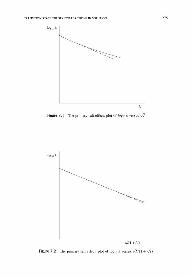
I
log10 k
Figure 7.1 The primary salt effect: plot of log10 k versusffiffiIp
log10 k
I/(1 + I)
Figure 7.2 The primary salt effect: plot of log10 k versusffiffiIp
=ð1þffiffiIpÞ
TRANSITION STATE THEORY FOR REACTIONS IN SOLUTION 275
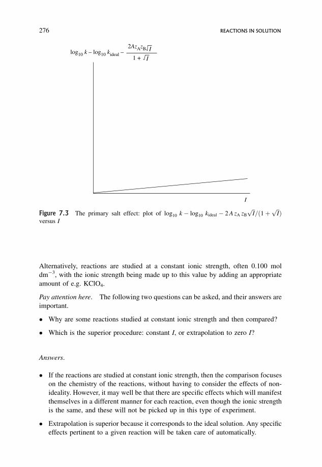
Alternatively, reactions are studied at a constant ionic strength, often 0.100 mol
dm�3, with the ionic strength being made up to this value by adding an appropriate
amount of e.g. KClO4.
Pay attention here. The following two questions can be asked, and their answers are
important.
� Why are some reactions studied at constant ionic strength and then compared?
� Which is the superior procedure: constant I, or extrapolation to zero I?
Answers.
� If the reactions are studied at constant ionic strength, then the comparison focuses
on the chemistry of the reactions, without having to consider the effects of non-
ideality. However, it may well be that there are specific effects which will manifest
themselves in a different manner for each reaction, even though the ionic strength
is the same, and these will not be picked up in this type of experiment.
� Extrapolation is superior because it corresponds to the ideal solution. Any specific
effects pertinent to a given reaction will be taken care of automatically.
I
log10 k _ log10 kideal _
I 2AzAzB
I 1 +
Figure 7.3 The primary salt effect: plot of log10 k � log10 kideal � 2 A zA zB
ffiffiIp
=ð1þffiffiIpÞ
versus I
276 REACTIONS IN SOLUTION
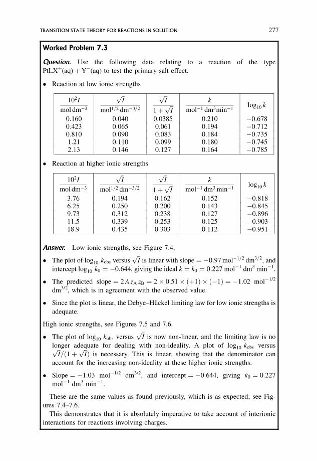
Worked Problem 7.3
Question. Use the following data relating to a reaction of the type
PtLXþ(aq)þY�(aq) to test the primary salt effect.
� Reaction at low ionic strengths
102I
mol dm�3
ffiffiIp
mol1=2 dm�3=2
ffiffiIp
1þffiffiIp k
mol�1 dm3min�1log10 k
0:160 0:040 0:0385 0:210 �0:6780:423 0:065 0:061 0:194 �0:7120:810 0:090 0:083 0:184 �0:7351:21 0:110 0:099 0:180 �0:7452:13 0:146 0:127 0:164 �0:785
� Reaction at higher ionic strengths
102I
mol dm�3
ffiffiIp
mol1=2 dm�3=2
ffiffiIp
1þffiffiIp k
mol�1 dm3 min�1log10 k
3:76 0:194 0:162 0:152 �0:8186:25 0:250 0:200 0:143 �0:8459:73 0:312 0:238 0:127 �0:89611:5 0:339 0:253 0:125 �0:90318:9 0:435 0:303 0:112 �0:951
Answer. Low ionic strengths, see Figure 7.4.
� The plot of log10 kobs versusffiffiIp
is linear with slope ¼ �0:97 mol�1=2 dm3=2, and
intercept log10 k0 ¼ �0:644, giving the ideal k ¼ k0 ¼ 0:227 mol�1 dm3 min�1.
� The predicted slope ¼ 2 A zA zB ¼ 2 0:51 ðþ1Þ ð�1Þ ¼ �1:02 mol�1/2
dm3/2, which is in agreement with the observed value.
� Since the plot is linear, the Debye–Huckel limiting law for low ionic strengths is
adequate.
High ionic strengths, see Figures 7.5 and 7.6.
� The plot of log10 kobs versusffiffiIp
is now non-linear, and the limiting law is no
longer adequate for dealing with non-ideality. A plot of log10 kobs versusffiffiIp
=ð1þffiffiIpÞ is necessary. This is linear, showing that the denominator can
account for the increasing non-ideality at these higher ionic strengths.
� Slope ¼ �1:03 mol�1/2 dm3/2, and intercept ¼ �0:644, giving k0 ¼ 0:227
mol�1 dm3 min�1.
These are the same values as found previously, which is as expected; see Fig-
ures 7.4–7.6.
This demonstrates that it is absolutely imperative to take account of interionic
interactions for reactions involving charges.
TRANSITION STATE THEORY FOR REACTIONS IN SOLUTION 277
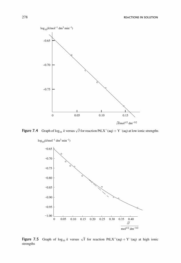
_0.65
_0.70
_0.75
0 0.05 0.10 0.15
log10(k/mol_1 dm3 min
_1)
I/mol1/2 dm_3/2
Figure 7.4 Graph of log10 k versusffiffiIp
for reaction PtLXþ(aq)þY�(aq) at low ionic strengths
_0.65
_0.70
_0.75
_0.80
_0.85
_0.90
_0.95
_1.000 0.05 0.10 0.15 0.20 0.25 0.30 0.35 0.40
log10(k/mol_1 dm3 min
_1)
mol1/2 dm_3/2
I
Figure 7.5 Graph of log10 k versusffiffiIp
for reaction PtLXþ(aq)þY�(aq) at high ionic
strengths
278 REACTIONS IN SOLUTION
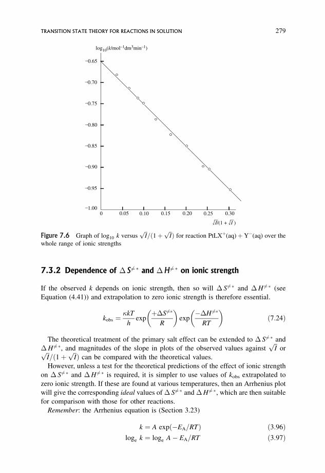
7.3.2 Dependence of � S 6¼ � and �H 6¼ � on ionic strength
If the observed k depends on ionic strength, then so will � S6¼ � and �H 6¼ � (see
Equation (4.41)) and extrapolation to zero ionic strength is therefore essential.
kobs ¼�kT
hexp
þ�S6¼�
R
� �exp
��H 6¼�
RT
� �ð7:24Þ
The theoretical treatment of the primary salt effect can be extended to � S6¼ � and
�H 6¼ �, and magnitudes of the slope in plots of the observed values againstffiffiIp
orffiffiIp
=ð1þffiffiIpÞ can be compared with the theoretical values.
However, unless a test for the theoretical predictions of the effect of ionic strength
on � S6¼ � and �H 6¼ � is required, it is simpler to use values of kobs extrapolated to
zero ionic strength. If these are found at various temperatures, then an Arrhenius plot
will give the corresponding ideal values of � S6¼ � and �H 6¼ �, which are then suitable
for comparison with those for other reactions.
Remember: the Arrhenius equation is (Section 3.23)
k ¼ A expð�EA=RTÞ ð3:96Þloge k ¼ loge A� EA=RT ð3:97Þ
_0.65
_0.70
_0.75
_0.80
_0.85
_0.90
_0.95
_1.000 0.05 0.10 0.15 0.20 0.25 0.30
log10(k/mol–1dm3min–1)
I/(1 + I )
Figure 7.6 Graph of log10 k versusffiffiIp
=ð1þffiffiIpÞ for reaction PtLXþ(aq)þY�(aq) over the
whole range of ionic strengths
TRANSITION STATE THEORY FOR REACTIONS IN SOLUTION 279
and a plot of loge k versus 1/T should be linear with slope ¼ �EA=RT and
intercept ¼ loge A.
7.3.3 The effect of the solvent
The ideal k (corresponding to the extrapolated value at zero ionic strength) should
always be used when the effect of solvent is considered, especially for ion–ion and
ion–molecule reactions.
Equation (4.39) is the simplest starting point for the simplified treatment for non-
ideality, but Equation (4.40) is the simplest starting point for the effect of the solvent
on the observed rate constant, though it can also be used to derive the effect of non-
ideality.
k ¼ � kT
hexp
��G6¼ �
k T
� �ð7:25Þ
This is Equation (4.40) re-written with �G 6¼� expressed as a molecular instead of a
molar quantity, and so k, the Boltzmann constant, is used instead of R, the gas
constant.
For reactions in solution, the exponential term appropriate to the gas phase has to
be modified to include the contribution accounting for the charges and the solvent.
Calculations show that �G6¼ � has to be modified by a term involving "r, the relative
permittivity of the solvent, and the charges on the ions. This term turns out to be the
same as that appearing in the collision formula, Equation (7.3), i.e. zAzBe2=4�"0 "r r6¼, so that
�G6¼ �ions in solution ¼ �G
6¼ �molecules in gas þ
zAzB e2
4�"0"r r6¼ð7:26Þ
The fact that the same expression modifies both collision theory and transition state
theory should not cause surprise. This is because the modification is taking account of
the same physical phenomenon in both theories, i.e. the interaction between the ions.
Equation (7.26) modifies the free energy of activation for a reaction between
molecules in the gas phase by making allowance for the effects of the charges and the
solvent only. A further modification allows for the effects of non-ideality, and ends up
with the same dependence of �G6¼ �ions in solution on ionic strength as results from the
simpler approach given in Section 7.3.1.
Equation (7.26) must only be used to discuss reactions under ideal conditions and
only applies to data extrapolated to zero ionic strength.
Since
k ¼ �kT
hexp
��G6¼�
kT
� �ð7:25Þ
280 REACTIONS IN SOLUTION
then
loge kidealions in solution ¼ loge
�kT
h��G
6¼�molecules in gas
kT� zA zB e2
4� "0 "r r6¼ kTð7:27Þ
If all other variables are kept constant, then a decrease in "r will cause a decrease in k
if zA zB is positive, and will cause an increase if zA zB is negative. However, this
assumes that r6¼ does not change as the permittivity changes. This is probably not
justifiable.
The predicted loge kobs ¼ loge kidealions in solution depends linearly on 1="r for a given
temperature, provided r6¼ is the same in all solvents. If extrapolated experimental
loge kidealobs values for a variety of solvents, and corresponding to zero ionic strength,
i.e. an ideal solution, are plotted against 1="r, then predicted slope ¼ �zAzB e2=
4� "0 r6¼ kT . This can be compared with the observed slope.
This equation predicts that
� if the reacting ions are of like sign then the slope is negative;
� if the reacting ions are of unlike sign then the slope is positive;
� if r6¼ varies with the solvent, then the value of the slope is unpredictable, and the
experimental points may not even lie on a common straight line or curve.
However, it is not reasonable to assume that r6¼ should be the same for a given
reaction under all circumstances, for the following reasons.
(a) r6¼ is the distance between the charges in the activated complex. As the relative
permittivity decreases, the effect of associative phenomena increases, as does the
possibility of clustering of solvent molecules and of charges, so the solvent has
an effect on r6¼.
(b) Temperature could also have an effect on r6¼, e.g. by decreasing the effect of
interactions between the charged species as the thermal energy becomes greater
than or equal to the electrostatic energy of interaction.
� The experimental slope can be compared with the theoretical value. If it is
assumed that the theory holds, then a comparison should give values of r 6¼, which
can then be used to infer something about the structure and solvation pattern of the
activated complex.
� The treatment assumes that the solvent is microscopically homogeneous. This
need not happen with mixed solvents.
� This equation is approximate since it assumes that the solvent is a structureless
continuum, and so cannot interact with the reactants and the activated complex.
Electrolyte solution studies demonstrate conclusively that this is not the case. In
TRANSITION STATE THEORY FOR REACTIONS IN SOLUTION 281
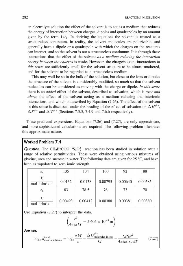
an electrolyte solution the effect of the solvent is to act as a medium that reduces
the energy of interaction between charges, dipoles and quadrupoles by an amount
given by the term 1="r. In deriving the equations the solvent is treated as a
structureless continuum. In reality, the solvent molecules are polarizable, and
generally have a dipole or a quadrupole with which the charges on the reactants
can interact, and so the solvent is not a structureless continuum. It is through these
interactions that the effect of the solvent as a medium reducing the interaction
energy between the charges is made. However, the charge/solvent interactions in
this sense are sufficiently small for the solvent structure to be almost unaltered,
and for the solvent to be regarded as a structureless medium.
This may well be so in the bulk of the solution, but close to the ions or dipoles
the structure of the solvent is considerably modified, so much so that the solvent
molecules can be considered as moving with the charge or dipole. In this sense
there is an added effect of the solvent, described as solvation, which is over and
above the effect of the solvent acting as a medium reducing the interionic
interactions, and which is described by Equation (7.26). The effect of the solvent
in this sense is discussed under the heading of the effect of solvation on �H 6¼ �,� S6¼ � and �V 6¼ � (Sections 7.5.5, 7.4.9 and 7.6.6 respectively).
These predicted expressions, Equations (7.26) and (7.27), are only approximate,
and more sophisticated calculations are required. The following problem illustrates
this approximate nature.
Worked Problem 7.4
Question. The CH2BrCOO�/S2O2�3 reaction has been studied in solution over a
range of relative permittivities. These were obtained using various mixtures of
glycine, urea and sucrose in water. The following data are given for 25 �C, and have
been extrapolated to zero ionic strength.
"r 135 134 100 92 88
k
mol�1dm3s�1 0:0132 0:0138 0:00795 0:00640 0:00585
"r 83 78:5 76 73 70
k
mol�1dm3s�10:00493 0:00412 0:00388 0:00381 0:00380
Use Equation (7.27) to interpret the data.
e2
4�"0 kT¼ 5:605 10�8 m
� �
Answer.
loge kidealions in solution ¼ loge
� kT
h��G
6¼ �molecules in gas
kT� zAzBe2
4�"0"rr6¼ kTð7:27Þ
282 REACTIONS IN SOLUTION
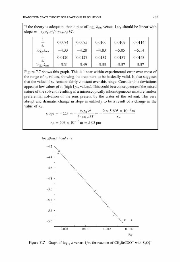
If the theory is adequate, then a plot of loge kobs versus 1="r should be linear with
slope ¼ �zA zB e2=4� "0 r6¼ kT:
1
"r
0:0074 0:0075 0:0100 0:0109 0:0114
loge kobs �4:33 �4:28 �4:83 �5:05 �5:141
"r
0:0120 0:0127 0:0132 0:0137 0:0143
loge kobs �5:31 �5:49 �5:55 �5:57 �5:57
Figure 7.7 shows this graph. This is linear within experimental error over most of
the range of "r values, showing the treatment to be basically valid. It also suggests
that the value of r6¼ remains fairly constant over this range. Considerable deviations
appear at low values of "r (high 1="r values). This could be a consequence of the mixed
nature of the solvent, resulting in a microscopically inhomogeneous mixture, and/or
preferential solvation of the ions present by the water of the solvent. The very
abrupt and dramatic change in slope is unlikely to be a result of a change in the
value of r6¼.
slope ¼ �223 ¼ � zAzB e2
4�"0r6¼ kT¼ � 2 5:605 10�8 m
r6¼
r6¼ ¼ 503 10�10 m ¼ 5:03 pm
_4.2
_4.4
_4.6
_4.8
_5.0
_5.2
_5.4
_5.6
0.0140.0120.0100.008
log10(k/mol_1 dm3 s_1)
1/εr
Figure 7.7 Graph of log10 k versus 1="r for reaction of CH2BrCOO� with S2O2�3
TRANSITION STATE THEORY FOR REACTIONS IN SOLUTION 283
7.3.4 Extension to include the effect of non-ideality
If the effect of non-ideality due to long range interionic interactions is included, then
it follows from Equation (7.25) that for any one solvent
log10 knon-idealions in solution ¼ log10 k0 þ 2 A zA zB
ffiffiIp
ð7:28Þ
which is the same as Equation (7.21), deduced by the more straightforward procedure.
Extensions to higher ionic strength give Equations (7.22) and (7.23).
7.3.5 Deviations from predicted behaviour
The following are the major sources of deviations from predicted behaviour.
� Ion association and other associative phenomena are not discussed. It is vital that
such effects are considered, especially at higher ionic strengths, where significant
association occurs. In kinetic studies, allowances for ion pairing are made by
distinguishing between the stoichiometric ionic concentrations and the actual
ones.
Note. The stoichiometric concentration is that based on the amount of the solute
weighed out and the volume of the solution, i.e. it assumes that the solute in solution
corresponds to that indicated by the formula.
The actual concentration takes account of the fact that the solute may alter
character when in solution, e.g. the undissociated solute may be partially ionized
in solution, or the free ions of an electrolyte may be partially removed to form ion
pairs.
Kinetic results which apparently do not fit the above treatment of the primary salt
effect do so when the observed rates are correlated with the actual ionic strengths
rather than the stoichiometric values. The actual concentrations in the reaction
solution are calculated using the known value of the equilibrium constant describing
the ion pair. This is discussed in Problem 7.5.
Note. Ion pairing results when the electrostatic interactions between two oppositely
charged ions become sufficiently large for the two ions to move around as one entity,
the ion pair; e.g., in solutions of Na2SO4, the following occurs:
NaþðaqÞ þ SO2�4 ðaqÞ ! � NaSO�4 ðaqÞ
The NaþðaqÞ is distributed between free Naþ and the ion pair NaSO�4 , so that
½Naþ�total ¼ ½Naþ�actual þ ½NaSO�4 �actual ð7:29Þ
and the total concentration is equivalent to the stoichiometric value. Total
and stoichiometric are in this sense interchangeable. The same argument can be
284 REACTIONS IN SOLUTION
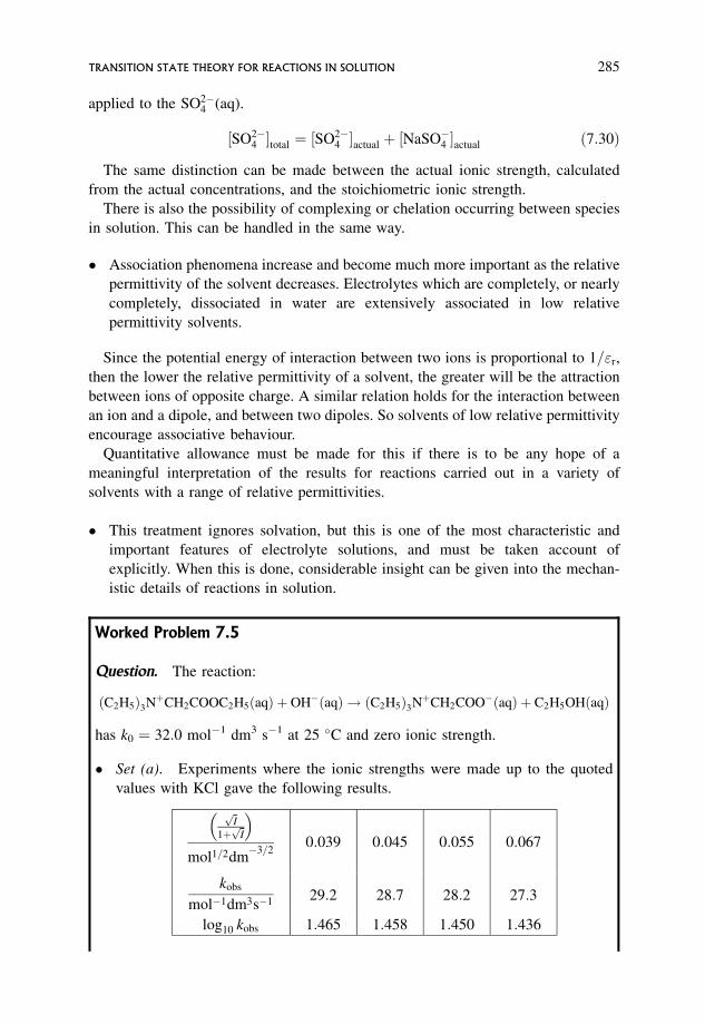
applied to the SO2�4 (aq).
½SO2�4 �total ¼ ½SO2�
4 �actual þ ½NaSO�4 �actual ð7:30Þ
The same distinction can be made between the actual ionic strength, calculated
from the actual concentrations, and the stoichiometric ionic strength.
There is also the possibility of complexing or chelation occurring between species
in solution. This can be handled in the same way.
� Association phenomena increase and become much more important as the relative
permittivity of the solvent decreases. Electrolytes which are completely, or nearly
completely, dissociated in water are extensively associated in low relative
permittivity solvents.
Since the potential energy of interaction between two ions is proportional to 1="r,
then the lower the relative permittivity of a solvent, the greater will be the attraction
between ions of opposite charge. A similar relation holds for the interaction between
an ion and a dipole, and between two dipoles. So solvents of low relative permittivity
encourage associative behaviour.
Quantitative allowance must be made for this if there is to be any hope of a
meaningful interpretation of the results for reactions carried out in a variety of
solvents with a range of relative permittivities.
� This treatment ignores solvation, but this is one of the most characteristic and
important features of electrolyte solutions, and must be taken account of
explicitly. When this is done, considerable insight can be given into the mechan-
istic details of reactions in solution.
Worked Problem 7.5
Question. The reaction:
ðC2H5Þ3NþCH2COOC2H5ðaqÞ þ OH�ðaqÞ ! ðC2H5Þ3NþCH2COO�ðaqÞ þ C2H5OHðaqÞ
has k0 ¼ 32:0 mol�1 dm3 s�1 at 25 �C and zero ionic strength.
� Set (a). Experiments where the ionic strengths were made up to the quoted
values with KCl gave the following results.
ffiffiIp
1þffiffiIp
� �
mol1=2dm�3=2
0:039 0:045 0:055 0:067
kobs
mol�1dm3s�1 29:2 28:7 28:2 27:3
log10 kobs 1:465 1:458 1:450 1:436
TRANSITION STATE THEORY FOR REACTIONS IN SOLUTION 285
ffiffiIp
1þffiffiIp
� �
mol1=2dm�3=2
0:090 0:120 0:139 0:158
kobs
mol�1dm3s�1 25:8 24:1 23:0 22:0
log10 kobs 1:412 1:382 1:362 1:342
� Set (b). Experiments at high ionic strengths in the presence of various
concentrations of CaCl2 gave the following results.
ffiffiIp
1þffiffiIp
� �
mol1=2dm�3=2
0:090 0:120 0:139 0:158
kobs
mol�1dm3s�1 25:2 22:8 21:3 20:1
log10 kobs 1:401 1:358 1:328 1:303
� Set (c). Experiments at low ionic strengths in the presence of various
concentrations of CaCl2, gave the following results.
ffiffiIp
1þffiffiIp
� �
mol1=2dm�3=2
0:039 0:045 0:055 0:067
kobs
mol�1dm3s�1 29:2 28:6 27:9 26:8
log10 kobs 1:465 1:456 1:446 1:428
Interpret the data.
Answer.
� For set (a) data, for reactions in the absence of Ca2þ, a plot of log10 kobs
versusffiffiIp
=ð1þffiffiIpÞ is linear with slope ¼ �1:03 mol�1/2 dm3/2, which agrees
with the predicted slope of 2 A zA zB ¼ þ2 0:510 ðþ1Þ ð�1Þ mol�1/2
dm3/2, i.e. �1.02 mol�1/2 dm3/2.
Intercept ¼ log10 k0 ¼ 1:505, giving the ideal k0 ¼ 32:0 mol�1 dm3 s�1
(Figure 7.8(a)).
This confirms the essential correctness of the theoretical treatment of the
primary salt effect.
� For the second set of data, set (b), for reactions in the presence of Ca2þ, but
at high ionic strengths, the plot of log10 kobs versusffiffiIp
=ð1þffiffiIpÞ is also linear,
but there are several features that do not fit with the theoretical predictions
(Figure 7.8(b)).
286 REACTIONS IN SOLUTION
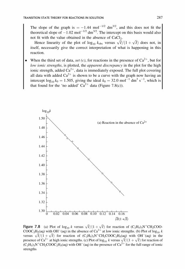
The slope of the graph is ¼ �1:44 mol�1/2 dm3/2, and this does not fit the
theoretical slope of �1:02 mol�1/2 dm3/2. The intercept on this basis would also
not fit with the value obtained in the absence of CaCl2.
Hence linearity of the plot of log10 kobs versusffiffiIp
=ð1þffiffiIpÞ does not, in
itself, necessarily give the correct interpretation of what is happening in this
reaction.
� When the third set of data, set (c), for reactions in the presence of Ca2þ, but for
low ionic strengths, is plotted, the apparent discrepancy in the plot for the high
ionic strength, added Ca2þ, data is immediately exposed. The full plot covering
all data with added Ca2þ is shown to be a curve with the graph now having an
intercept log10 k0 ¼ 1:505, giving the ideal k0 ¼ 32:0 mol�1 dm3 s�1, which is
that found for the ‘no added’ Ca2þ data (Figure 7.8(c)).
1.50
1.48
1.46
1.44
1.42
1.40
1.38
1.36
1.34
1.32
1.300 0.02 0.04 0.06 0.08 0.10 0.12 0.14 0.16
log10k
(a) Reaction in the absence of Ca2+
I/(1 + I)
Figure 7.8 (a) Plot of log10 k versusffiffiIp
=ð1þffiffiIpÞ for reaction of (C2H5)3NþCH2COO-
COOC2H5(aq) with OH�(aq) in the absence of Ca2þ at low ionic strengths. (b) Plot of log10 k
versusffiffiIp
=ð1þffiffiIpÞ for reaction of (C2H5)3NþCH2COOC2H5(aq) with OH�(aq) in the
presence of Ca2þ at high ionic strengths. (c) Plot of log10 k versusffiffiIp
=ð1þffiffiIpÞ for reaction of
(C2H5)3NþCH2COOC2H5(aq) with OH�(aq) in the presence of Ca2þ for the full range of ionic
strengths
TRANSITION STATE THEORY FOR REACTIONS IN SOLUTION 287
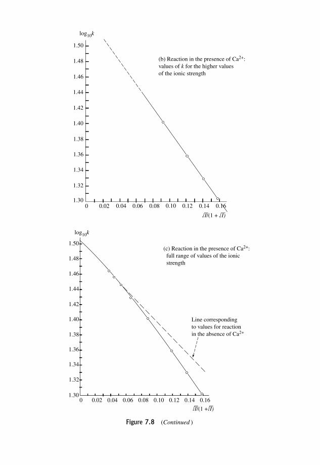
1.50
1.48
1.46
1.44
1.42
1.40
1.38
1.36
1.34
1.32
0.020 0.04 0.06 0.08 0.10 0.12 0.14 0.161.30
(b) Reaction in the presence of Ca2+:values of k for the higher valuesof the ionic strength
I/(1 + I)
log10k
log10k
1.50
1.48
1.46
1.44
1.42
1.40
1.38
1.36
1.34
1.32
0.02 0.04 0.06 0.08 0.10 0.12 0.14 0.161.30
0
Line correspondingto values for reactionin the absence of Ca2+
(c) Reaction in the presence of Ca2+: full range of values of the ionic strength
I/(1 + I)
Figure 7.8 (Continued )
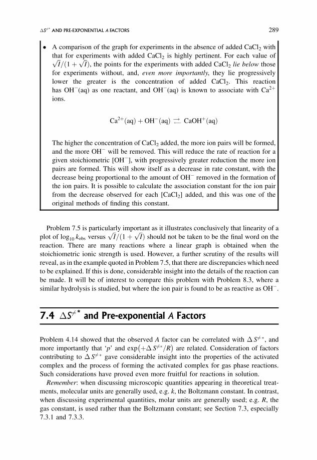
� A comparison of the graph for experiments in the absence of added CaCl2 with
that for experiments with added CaCl2 is highly pertinent. For each value offfiffiIp
=ð1þffiffiIpÞ, the points for the experiments with added CaCl2 lie below those
for experiments without, and, even more importantly, they lie progressively
lower the greater is the concentration of added CaCl2. This reaction
has OH�(aq) as one reactant, and OH�(aq) is known to associate with Ca2þ
ions.
Ca2þðaqÞ þ OH�ðaqÞ ! � CaOHþðaqÞ
The higher the concentration of CaCl2 added, the more ion pairs will be formed,
and the more OH� will be removed. This will reduce the rate of reaction for a
given stoichiometric [OH�], with progressively greater reduction the more ion
pairs are formed. This will show itself as a decrease in rate constant, with the
decrease being proportional to the amount of OH� removed in the formation of
the ion pairs. It is possible to calculate the association constant for the ion pair
from the decrease observed for each [CaCl2] added, and this was one of the
original methods of finding this constant.
Problem 7.5 is particularly important as it illustrates conclusively that linearity of a
plot of log10 kobs versusffiffiIp
=ð1þffiffiIpÞ should not be taken to be the final word on the
reaction. There are many reactions where a linear graph is obtained when the
stoichiometric ionic strength is used. However, a further scrutiny of the results will
reveal, as in the example quoted in Problem 7.5, that there are discrepancies which need
to be explained. If this is done, considerable insight into the details of the reaction can
be made. It will be of interest to compare this problem with Problem 8.3, where a
similar hydrolysis is studied, but where the ion pair is found to be as reactive as OH�.
7.4 �S 6¼* and Pre-exponential A Factors
Problem 4.14 showed that the observed A factor can be correlated with � S6¼ �, and
more importantly that ‘p’ and exp þ� S6¼�=R �
are related. Consideration of factors
contributing to � S6¼ � gave considerable insight into the properties of the activated
complex and the process of forming the activated complex for gas phase reactions.
Such considerations have proved even more fruitful for reactions in solution.
Remember: when discussing microscopic quantities appearing in theoretical treat-
ments, molecular units are generally used, e.g. k, the Boltzmann constant. In contrast,
when discussing experimental quantities, molar units are generally used; e.g. R, the
gas constant, is used rather than the Boltzmann constant; see Section 7.3, especially
7.3.1 and 7.3.3.
�S 6¼* AND PRE-EXPONENTIAL A FACTORS 289
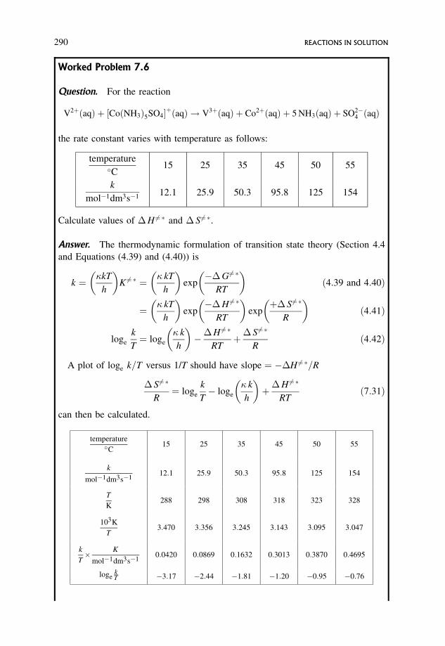
Worked Problem 7.6
Question. For the reaction
V2þðaqÞ þ ½CoðNH3Þ5SO4�þðaqÞ ! V3þðaqÞ þ Co2þðaqÞ þ 5 NH3ðaqÞ þ SO2�4 ðaqÞ
the rate constant varies with temperature as follows:
temperature�C
15 25 35 45 50 55
k
mol�1dm3s�1 12:1 25:9 50:3 95:8 125 154
Calculate values of �H 6¼ � and � S6¼ �.
Answer. The thermodynamic formulation of transition state theory (Section 4.4
and Equations (4.39) and (4.40)) is
k ¼ �kT
h
� �K 6¼ � ¼ � kT
h
� �exp
��G6¼ �
RT
� �ð4:39 and 4:40Þ
¼ � kT
h
� �exp
��H 6¼ �
RT
� �exp
þ� S6¼ �
R
� �ð4:41Þ
loge
k
T¼ loge
� k
h
� ���H 6¼ �
RTþ� S6¼ �
Rð4:42Þ
A plot of loge k=T versus 1/T should have slope ¼ ��H 6¼ �=R
� S6¼ �
R¼ loge
k
T� loge
� k
h
� �þ�H 6¼ �
RTð7:31Þ
can then be calculated.
temperature�C
15 25 35 45 50 55
k
mol�1dm3s�112:1 25:9 50:3 95:8 125 154
T
K288 298 308 318 323 328
103K
T3:470 3:356 3:245 3:143 3:095 3:047
k
T K
mol�1dm3s�10:0420 0:0869 0:1632 0:3013 0:3870 0:4695
logekT �3:17 �2:44 �1:81 �1:20 �0:95 �0:76
290 REACTIONS IN SOLUTION
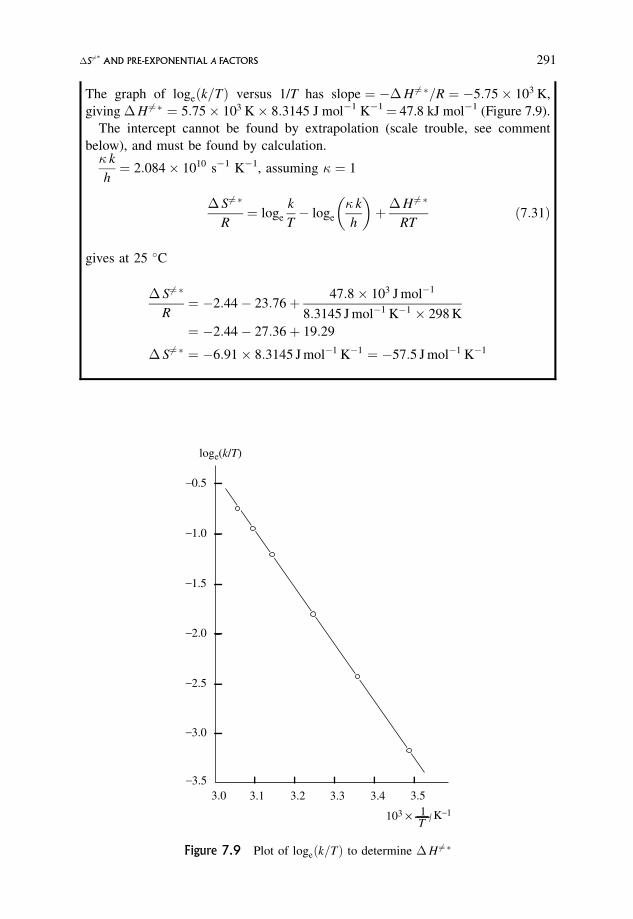
The graph of logeðk=TÞ versus 1/T has slope ¼ ��H 6¼ �=R ¼ �5:75 103 K,
giving �H 6¼ � ¼ 5:75 103 K 8:3145 J mol�1 K�1¼ 47.8 kJ mol�1 (Figure 7.9).
The intercept cannot be found by extrapolation (scale trouble, see comment
below), and must be found by calculation.� k
h¼ 2:084 1010 s�1 K�1, assuming � ¼ 1
� S6¼ �
R¼ loge
k
T� loge
� k
h
� �þ�H 6¼ �
RTð7:31Þ
gives at 25 �C
� S6¼ �
R¼ �2:44� 23:76þ 47:8 103 J mol�1
8:3145 J mol�1 K�1 298 K
¼ �2:44� 27:36þ 19:29
� S6¼ � ¼ �6:91 8:3145 J mol�1 K�1 ¼ �57:5 J mol�1 K�1
_0.5
_1.0
_1.5
_2.0
_2.5
_3.0
_3.53.0 3.1 3.2 3.3 3.4 3.5
loge(k/T)
103 × 1T / K
_1
Figure 7.9 Plot of logeðk=TÞ to determine �H 6¼ �
�S 6¼* AND PRE-EXPONENTIAL A FACTORS 291
7.4.1 A typical problem in graphical analysis
Problem 7.6 illustrates a procedural problem often encountered by students.
k ¼ � kT
h
� �K 6¼ � ¼ � kT
h
� �exp
��G6¼ �
RT
� �ð4:39Þ and ð4:40Þ
k
T¼ � k
h
� �exp
��H 6¼ �
RT
� �exp
þ� S6¼ �
R
� �ð7:32Þ
loge
k
T¼ loge
� k
h
� ���H 6¼ �
RTþ� S6¼ �
Rð4:42Þ
giving
� S 6¼ � ¼ R loge
k
T� R loge
� k
h
� �þ�H 6¼ �
Tð7:33Þ
A plot of logeðk=TÞ versus 1=T should have slope ¼ ��H 6¼ �=R.
When the plot of logeðk=TÞ versus 1=T is drawn, there is a very long extrapolation
to zero for 1=T. To carry out this extrapolation would require a ridiculous amount of
graph paper, or a ridiculous bunching together of points on ordinary graph paper.
Graphical extrapolation is impossible, and the value of the intercept must be found by
calculation. This can happen in various aspects of physical chemistry, and very often
occurs in plots vs 1=T .
7.4.2 Effect of the molecularity of the step for which � S 6¼ � is found
As in the gas phase, if the reaction step is bimolecular with two species forming an
activated complex resembling a single species, there will be a decrease in entropy
on activation. In solution this is called an associative reaction. If reaction is
unimolecular and the activated complex resembles an incipient two (or more) species,
then an increase in entropy would result. This is termed a dissociative reaction for
solution reactions. A reaction somewhere in between these two extremes is termed
interchange, and the entropy change is likely to be small.
7.4.3 Effect of complexity of structure
In the gas phase it was shown that as the complexity of the reacting molecules
increased, � S6¼ � decreased; see Sections 4.3.5 and 4.4.2. This is a consequence
of including the effect of the internal motions of rotation and vibration in reactants
and activated complex. The change in the number of degrees of freedom is a major
contribution to the entropy of activation; see Problems 4.12–4.15.
292 REACTIONS IN SOLUTION
7.4.4 Effect of charges on reactions in solution
One of the most characteristic features of reactions in solution which involve ionic
charges in reactants, or a charge distribution in the activated complex, is the quite
decided dependence of the A factor on the charges involved. This has been hinted at
previously in Section 7.1. Electrostatic interactions are important both between the
reacting species themselves, and also especially with the solvent. This is not limited
to reactions involving ionic species. Two neutral polar molecules can easily give a
charge-separated activated complex which, though neutral overall, has an uneven
distribution of charge over it.
7.4.5 Effect of charge and solvent on � S6¼ � for ion–ion reactions
The following does not include the effect of solvation and the change in the structure
of the solvent on activation. This is discussed independently in Section 7.4.9.
For ideal conditions, corresponding to rate constants extrapolated to zero ionic
strength,
�G6¼ �ions in solution ¼ �G
6¼ �molecules in gas þ
zAzBe2
4�"0"rr6¼ð7:26Þ
Since reactions should be compared under ideal conditions, equation (7.26) is used.
The effect of temperature on �G6¼ � allows � S6¼ � to be found, since
� S 6¼ � ¼ � @�G6¼ �
@ T
� �p
ð7:34Þ
However, for reactions in solution it is necessary to consider also the fact that the
relative permittivity "r decreases as temperature increases. Thus, for ions of like
charge (zAzB positive), the electrostatic term in Equation (7.26) increases as T
increases. This gives a positive contribution to @�G 6¼ �=@ T �
p, and therefore a
negative contribution to � S6¼ �. Consequently, � S6¼ � is predicted to be less than the
value it would have taken if there had been no electrostatic term.
From such arguments it can be shown that Equation (7.26) gives the following
relations.
� For ions of like charge (zA zB positive), � S 6¼ � is predicted to be less than the value
which it would have taken if there had been no electrostatic term.
� For ions of unlike charge (zA zB negative), � S6¼ � is predicted to be greater than the
value which it would have taken if there had been no electrostatic term.
� For ions of like sign � S6¼ �ions in solution < � S
6¼ �molecules in gas.
�S 6¼* AND PRE-EXPONENTIAL A FACTORS 293
� For ions of unlike sign � S6¼ �ions in solution > � S
6¼ �molecules in gas.
Values of the A factor differ from each other because of differences in � S6¼ � (Worked
Problem 4.14). Because A is proportional to exp � S6¼ �=R �
, a larger value of � S6¼ �
means that there will be a larger value of A, and a smaller value of � S6¼ � means that
there will be a smaller value of A. Thus
� for ions of like sign, the relation
� S6¼ �ions in solution < � S
6¼ �molecules in gas
requires that
Aions in solution < Amolecules in gas
and so
log10 Aions in solution < log10 Amolecules in gas
� for ions of unlike sign, the relation
� S6¼ �ions in solution > � S
6¼ �molecules in gas
requires that
Aions in solution > Amolecules in gas
and so
log10 Aions in solution > log10 Amolecules in gas
For both these situations a choice will have to be made as to the magnitude of
Amolecules in gas, as this is the point of comparison. This is often taken to be around
3 1010 mol�1 dm3 s�1, log10 A ¼ 10:5.
Table 7.1 lists values of log10 A for some ionic reactions, and shows qualitative
agreement of experiment with this electrostatically modified collision theory. At first
sight this indicates the correctness of the electrostatic treatment.
However, a closer look shows that most of the reactions quoted are reactions of
polyatomic ions, where it could be expected that the internal rotational and
vibrational structures of the reactant ions and the activated complex will make a
significant contribution. Values of gas phase � S6¼ � (Table 4.4) become increasingly
more negative as the complexity of the reactants increases, with the corresponding
calculated p factors likewise becoming increasingly smaller. This indicates that there
cannot be a single point of comparison, and that there is considerable leeway in the
value which can be chosen.
The conclusion is that, unless the internal structure is included in the calculations,
or the point of comparison is chosen to take cognisance of this, the electrostatic
theory may not be adequate.
294 REACTIONS IN SOLUTION
7.4.6 Effect of charge and solvent on � S6¼ � for
ion–molecule reactions
Here there is a discrete charge on one of the reactants and a dipole on the other. The
electrostatic interactions arising from the charge and the solvent can be deduced
similarly to those for ion–ion interactions.
�G6¼ �ion--molecule in solution ¼ �G
6¼ �molecules in gas þ
ze� cos
4�"0"r r26¼
ð7:35Þ
where � is the dipole moment, and represents the angle of approach of the ion to the
dipole.
This gives the relation
� S6¼ �ion-dipole in solution > � S
6¼ �molecules in gas
from which it is predicted that Aion-dipole in solution > typical gas phase value, i.e.
>3 1010 mol�1 dm3 s�1. This prediction is qualitatively the same as that for
reaction between two ions of opposite charge. In physical terms, it arises because a
positive ion would usually approach the negative end of a dipole, and a negative ion
would usually approach the positive end of a dipole.
Detailed calculations suggest that p factors greater than unity and of the order of
1 to 103 are expected. This is not always observed; see Table 7.2, where some of the
reactions have p factors in the predicted range and some have p factors less than unity.
The above treatment needs to be modified in some way. It can again be asked
whether the typical value of A � 3 1010 mol�1 dm3 s�1 is the correct point of
comparison. If the lower values suggested by transition state theory become the point
of comparison, then the above treatment could be essentially correct.
Worked Problem 7.7
Question. Although there is a question as to whether A � 3 1010 mol�1 dm3
s�1 is the correct point of comparison for ion–molecule reactions, why is this
ambiguity less likely to be a problem for ion–ion reactions?
Answer. The argument in Section 7.4.6 suggests that the discrepancy between
predicted and observed values for ion–molecule reactions is a result of ignoring
the change in the internal degrees of freedom. This is also relevant to ion–ion
reactions when the ions are polyatomic species. But the charge effect for ion–
ion reactions / zA zB e2=r6¼ is much larger than the charge-dipole effect for ion–
molecule reactions / z e� cos =r26¼. It is a matter of the relative magnitudes of
these terms.
�S 6¼* AND PRE-EXPONENTIAL A FACTORS 295
7.4.7 Effect of charge and solvent on � S 6¼ � for
molecule–molecule reactions
The theoretical treatment here is even more fraught with difficulties than that for ion–
molecule reactions. Here, both the reactants and the activated complex are assumed to
be dipolar. The theory predicts that there will be a spread in the values of � S6¼ �
leading to p factors greater and less than unity, but these p factors are predicted to be
close to unity. The observed p factors vary over a large range, Table 7.3, and are
comparable to those for ion–ion-like charge reactions. The conclusion is that the
electrostatic treatment may be totally inadequate, or that the effects of the internal
structure are important.
7.4.8 Effects of changes in solvent on � S 6¼ �
It is much more difficult to predict the effect of change of solvent on � S6¼ � than it is
to predict the effect on the ideal rate constant. This is because the analysis for
the dependence of � S 6¼ � on solvent includes the temperature dependence of the
relative permittivity. This complexity in the analysis occurs for ion–ion and ion–
molecule reactions, and, because of the difficulty in disentangling the effects, this will
not be pursued further.
7.4.9 Changes in solvation pattern on activation, and the effect
on A factors for reactions involving charges and
charge-separated species in solution
A further complication in interpreting � S6¼ � values is the contribution made from
solvation, and the alteration of the structure of the solvent on activation. This is
dependent on the charges on the reactants and on the activated complex. The
activated complex has a charge equal to the algebraic sum of the charges on the
reactants.
Worked Problem 7.8
Question. Estimate the charges on the activated complexes formed during the
following reactions.
Question Answer
� þ3 charge reacting with þ1 charge þ4
� þ2 charge reacting with �1 charge þ1
� �1 charge reacting with �2 charge �3
296 REACTIONS IN SOLUTION
� �3 charge reacting with a þ1 charge �2
� þ2 charge reacting with a �2 charge zero overall,
but take care, the activated complex is probably still charge separated.
� �1 charge reacting with an uncharged molecule �1
� two uncharged molecules reacting with each other zero overall,
but take care, the activated complex could be charge separated.
For reactions involving charges and charge-separated species the solvent will be
orientated around the regions of charge, with the degree of orientation being greater
the greater the charge. Neutral species can still orientate the solvent around the
molecule by virtue of any asymmetric charge distribution, such as a dipole.
Worked Problem 7.9
Question. List the following species in order of ability to orientate solvent
molecules.
OH�; Ca2þ; H2O; H3Oþ; SO2�4 ; NHþ3 CH2COO�; CCl4; Al3þ
Answer.
Al3þ > Ca2þ � SO2�4 > OH� � H3Oþ > NHþ3 CH2COO� � H2O� CCl4
Note.
� NH3þCH2COO� is overall neutral, but charge separated;
� H2O is also overall neutral, but has only a dipole;
� CCl4 is also overall neutral, but has no dipole.
7.4.10 Reactions between ions in solution
Like charged ions Values of A: 102–108 dm3 mol�1s�1
Unlike charged ions Values of A: 1013–1019 dm3 mol�1s�1
There is very little variation in the magnitude of A for a given reaction in different
solvents.
�S 6¼* AND PRE-EXPONENTIAL A FACTORS 297
When reaction occurs between ions of like charge the activated complex will have
a larger charge than either reactant. All three will be solvated, but the activated
complex can orientate the solvent considerably more than can the reactant ions.
Orientation is equivalent to an increase in order for solvent molecules, which results
in an increase in order for the solvent on activation, manifesting itself as a decrease in
entropy on activation. Comparison with reactions for uncharged molecules in the gas
phase predicts a decreased value for the entropy of activation, and hence low A
factors.
When reaction is between ions of unlike sign the activated complex has a total net
charge less than the reactants, and so the total degree of orientation of the solvent
around the activated complex is now less than before activation. This leads to release
of solvent molecules giving an increase in disorder of the solvent, leading to an
increase in entropy on forming the activated complex. The � S6¼ � and the A factor are
predicted to be larger than the values found for the reaction of molecules in the gas
phase.
These predictions are confirmed by the typical values given in Table 7.1.
For both charge types it is not expected that there will be a great variation in � S6¼ �
and A with change of solvent, and experiment bears this out. The change in
orientation of solvent molecules on activation and the change of entropy are
irrespective of the ease with which the permanent dipoles of the solvent can be
oriented, even though there may be a wide spread in solvation of the reactant species
with change of solvent. What is important is that there will be a similar spread in
solvation of the activated complex with change of solvent, so there is little variation in
the change in orientation on activation with change of solvent.
For reactions between ions of like sign, solvation effects give a decrease in entropy
on activation. Consideration of the internal structure leads again to a decrease in
entropy on activation. The two effects reinforce each other, and also are in the same
direction as predicted by the electrostatic treatment as given in Section 7.4.5. This
would indicate p factors of less than unity.
For reactions between ions of unlike sign, solvation effects give an increase in
entropy on activation. Consideration of internal structure gives a decrease in � S6¼ �
and the two effects could balance, or partially balance, each other. The electrostatic
modifications would, however predict an increase in � S6¼ �, indicating p factors
greater than unity. Since the other two effects are in opposite directions to each other,
the electrostatic modifications must dominate, with this being the major factor
influencing the A factors.
7.4.11 Reaction between an ion and a molecule
Typical observed values of A are 109–1012 mol�1 dm3 s�1, with very little variation in
the magnitude of the A factor for a given reaction in different solvents.
The reactant molecule will be very much less solvated than the reactant ion,
while the activated complex will be solvated to a similar extent to the initial state
298 REACTIONS IN SOLUTION
since the total charge remains the same on activation. The net change in orientation of
the solvent will be small, giving a very small contribution to the entropy of activation
and to the A factor from solvation effects. A factors will lie in the gas phase range of
values. This is observed with a few exceptions (Table 7.2).
Since the total degree of orientation of the solvent is approximately the same for
the initial state and activated complex, the change in orientation is small and close to
zero, and approximately constant for a given reaction in a variety of solvents. Hence
A factors are not expected to vary much with change of solvent.
Table 7.2 shows these predictions to be borne out by a large number of reactions,
but there are exceptions where the A factors are much lower than expected. These can
be explained if the internal degrees of freedom are considered. Effects of electrostatic
interactions and of solvation are small, and could be in either direction, but the
dominant effect is probably due to internal motions.
7.4.12 Reactions between uncharged polar molecules
Typical observed values for A are 102–107 mol�1 dm3 s�1, and there is a large
variation for a given reaction in different solvents.
Here the reactants are overall neutral, though dipolar, and the activated complex is
also overall neutral. However, the charge distribution in the activated complex can
vary from dipolar to an incipient charge distribution similar to an ion pair, with a
range of different charge-separated intermediate structures possible. For instance, in
the reaction between tertiary amines and halogenoalkanes the product is an ionic
quaternary ammonium halide. For such reactions it is likely that the activated
complex will have considerable charge separation, even to the extent of resembling
an ion pair rather than a dipole:
R3Nþ R0I! ½R3N�þ----R0----I���6¼ ! R3R0NþI�
in contrast to reactions where molecular products are found, when the activated
complex could be merely dipolar.
Existence of charge distributed over the activated complex would encourage
solvation. The greater the degree of charge separation in the activated complex, the
greater will be the solvation. This gives increased orientation of the solvent on
activation and a decrease in entropy on activation. Hence low A factors are expected,
with lower values correlating with increasing charge separation and solvation in the
activated complex.
Since the reactants are molecules, the extent of solvation will be small and
approximately the same for all solvents. But the extent of charge separation in the
activated complex is very dependent on the solvent, by virtue of the magnitude of the
relative permittivity, and a large variation in the extent of solvation of the activated
complex is expected. The entropy of activation and the A factor are expected to vary
with change of solvent.
�S 6¼* AND PRE-EXPONENTIAL A FACTORS 299
Table 7.3 shows A factors that are much lower than theory would suggest and are
more in keeping with those for ions of like charge reacting. It seems reasonable to
assume that changes in the internal degrees of freedom are more important than are
the charge and solvent factors. This is in keeping with the similar situation for ion–
molecule reactions.
Worked Problem 7.10
Question. Assuming that the reaction step is associative, interpret the signs and
magnitudes of the � S6¼ � values for the following reactions in terms of charge and
complexity of structure:
Reaction� S6¼ �
J mol�1 K�1
Co(NH3)5Cl2þ(aq)þH2O(l) �32
Co(NH3)5(NO3)2þ(aq)þH2O(l) þ8
Pd(CN)2�4 (aq)þ CN�(aq) �178
PtdienBrþ(aq)þ I�(aq) �104
Co(NH3)5Br2þ(aq)þOH�(aq) þ92
V2þ(aq)þ Co(NH3)5SOþ4 (aq) �243
CH2BrCOO�(aq)þ S2O2�3 (aq) �71
CH3CONH2(aq)þH2O(l) �142
PtdienBrþ(aq)þ SCN�(aq) �112
(dien is NH2CH2CH2NHCH2CH2NH2.)
Answer.
Reaction� S6¼ �
J mol�1 K�1
Type of
reaction
Effect of
charge
Effect of
complexity
Effect of
solvation Comments
(a) Co(NH3)5Cl2þ(aq)þH2O(l)
�32 ionþdipole
small, and
þve
�ve:
perhaps
biggest
effect
small, þve
or �ve
seems to fit
(b) Co(NH3)5(NO3)2þ
(aq)þH2O(l)
þ8 ionþdipole
small, and
þve
�ve:
perhaps
biggest
effect
(similar to
(a))
small, þve
or �ve
does not fit, but
why the difference
from (a)?
�ve end of dipole
simulates
�ve charge under
influence of 2þ;
(þ2) þ (�1). This
effect would be
þve. But this
would apply to (a)
also?
300 REACTIONS IN SOLUTION
7.5 �H6¼* Values
Worked Problem 7.6 shows how �H 6¼ � values can be found from the temperature
dependence of the rate constant.
7.5.1 Effect of the molecularity of the step for which
the �H6¼ � value is found
Again a distinction is possible between associative, dissociative and interchange
mechanisms. In the dissociative mechanism at least one bond is broken. Dissocia-
tive reactions thus have higher �H 6¼ � values than associative mechanisms. Inter-
change mechanisms, where synchronous bond breaking and bond forming occur,
have values in between.
Reaction � S6¼ �
J mol�1 K�1
Type of
reaction
Effect of
charge
Effect of
complexity
Effect of
solvation Comments
(c) Pd(CN)42�(aq)þ
CN�(aq)
�178 (�2)þ(�1)
large, and
�ve
�ve �ve fits; complexity
enhances
(d) PtdienBrþ(aq)þI�(aq)
�104 (þ1)þ(�1)
þve large, and
�ve
þve does not fit:
complexity of dien
compensates
þve effects?
(e) Co(NH3)5Br2þ(aq)
þOH�(aq)
þ92 (þ2)þ(�1)
large, and
þve
�ve þve fits: complexity
reduces value?
(f) V2þ(aq)þCo(NH3)5SO4
þ(aq)
�243 (þ2)þ(þ1)
large, and
�ve
�ve �ve fits; compare with
(c)
(g) CH2BrCOO�(aq)þS2O2�
3 (aq)
�71 (�1)þ(�2)
large and
�ve
�ve �ve fits; compare with
(c) and (d)
(h) CH3CONH2(aq)þH2O(l)
�142 (0)þ (0) small,
possibly
�ve
small,
�ve
small,
possibly
�ve
does not fit:
mechanism may
involve initial
protonation
(i) PtdienBrþ(aq)þSCN�(aq)
�112 (þ1)þ(�1)
þve large, and
�ve
þve does not fit:
complexity of
dien compensates
þve effects?
compare
with (d)
This question demonstrates the variety of effects contributing to the observed
� S6¼ �, and indicates how to attempt to rationalize them. However, this analysis
assumes that the � S6¼ � values refer to a single associative step. A complete analysis
must include a full mechanistic study before any definitive conclusions are reached.
�H6¼* VALUES 301
7.5.2 Effect of complexity of structure
�H 6¼ � reflects the effect of bond breaking and bond making in the process of
activation. Although the internal motions will contribute to this, they will not be
expected to have a major effect.
7.5.3 Effect of charge and solvent on �H 6¼ � for ion–ion
and ion–molecule reactions
As in Sections 7.4.5 and 7.4.6, this does not include the effect of change in solvation
pattern. Equation (4.40) is the best starting point and leads to Equation (7.27) as given
in Section 7.3.3
loge
kidealions in solution
T¼ loge
� k
h��G
6¼ �molecules in gas
kT� zA zB e2
4� "0 "rr6¼ kTð7:36Þ
Since, by analogy with Equation (4.33),
�G6¼ � ¼ �H 6¼ � � T � S6¼ � ð7:37Þ
loge
kidealions in solution
T¼ loge
� k
hþ� S
6¼ �molecules in gas
R
��H
6¼ �molecules in gas
RT� zA zB e2
4� "0 "r r6¼ kTð7:38Þ
From this it can be shown that
for ions of like sign:�H
6¼ �ions in solution
R<
�H6¼ �molecules in gas
R
for ions of unlike sign:�H
6¼ �ions in solution
R>
�H6¼ �molecules in gas
R
An analogous treatment for reaction between an ion and a molecule suggests that
for reaction of an
ion with a molecule:�H
6¼�ionþmolecule in solution
R>
�H6¼ �molecules in gas
R
As with the treatment for � S6¼ �reactions in solution any comparisons with the gas phase
values depends critically on what value we choose for �H6¼ �molecules in gas.
302 REACTIONS IN SOLUTION
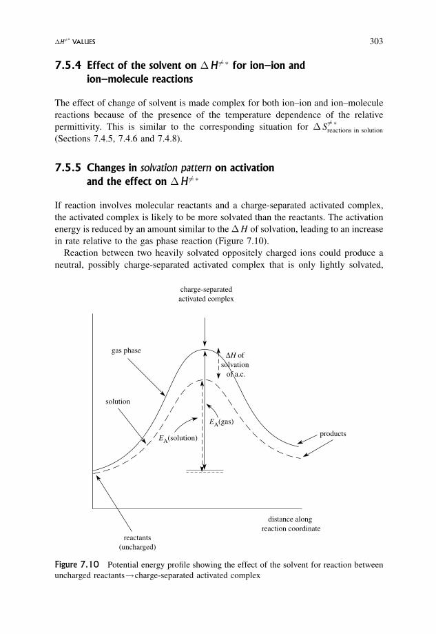
7.5.4 Effect of the solvent on �H 6¼ � for ion–ion and
ion–molecule reactions
The effect of change of solvent is made complex for both ion–ion and ion–molecule
reactions because of the presence of the temperature dependence of the relative
permittivity. This is similar to the corresponding situation for � S6¼ �reactions in solution
(Sections 7.4.5, 7.4.6 and 7.4.8).
7.5.5 Changes in solvation pattern on activation
and the effect on �H 6¼ �
If reaction involves molecular reactants and a charge-separated activated complex,
the activated complex is likely to be more solvated than the reactants. The activation
energy is reduced by an amount similar to the �H of solvation, leading to an increase
in rate relative to the gas phase reaction (Figure 7.10).
Reaction between two heavily solvated oppositely charged ions could produce a
neutral, possibly charge-separated activated complex that is only lightly solvated,
gas phase
charge-separatedactivated complex
distance along reaction coordinate
reactants(uncharged)
products
solution
EA(solution)
EA(gas)
∆H of solvation
of a.c.
Figure 7.10 Potential energy profile showing the effect of the solvent for reaction between
uncharged reactants!charge-separated activated complex
�H6¼* VALUES 303
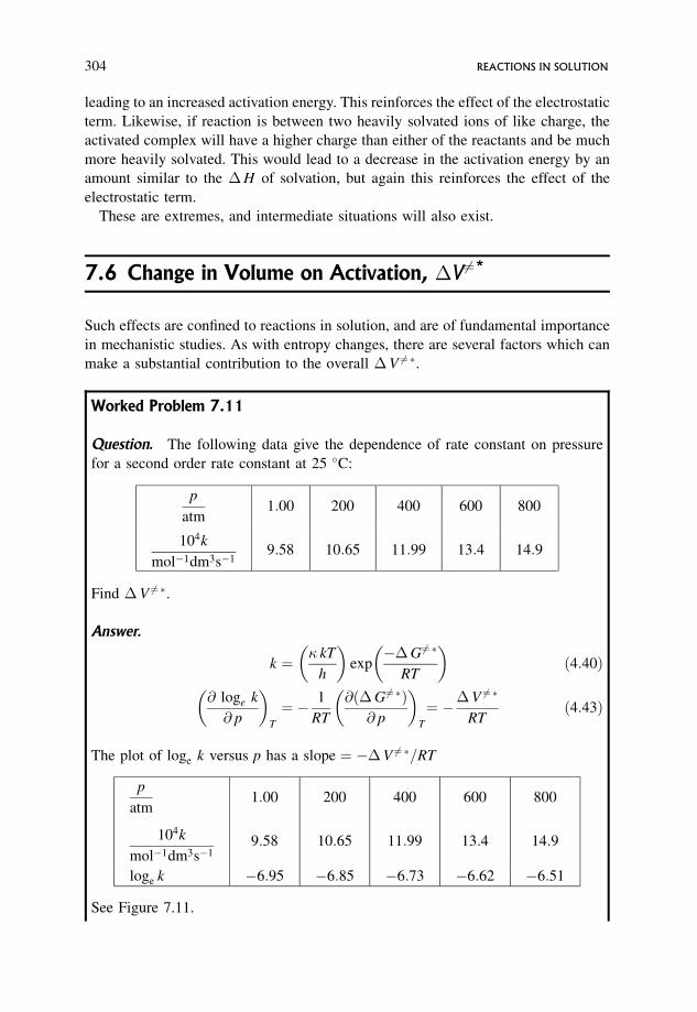
leading to an increased activation energy. This reinforces the effect of the electrostatic
term. Likewise, if reaction is between two heavily solvated ions of like charge, the
activated complex will have a higher charge than either of the reactants and be much
more heavily solvated. This would lead to a decrease in the activation energy by an
amount similar to the �H of solvation, but again this reinforces the effect of the
electrostatic term.
These are extremes, and intermediate situations will also exist.
7.6 Change in Volume on Activation, �V6¼*
Such effects are confined to reactions in solution, and are of fundamental importance
in mechanistic studies. As with entropy changes, there are several factors which can
make a substantial contribution to the overall �V 6¼ �.
Worked Problem 7.11
Question. The following data give the dependence of rate constant on pressure
for a second order rate constant at 25 �C:
p
atm1:00 200 400 600 800
104k
mol�1dm3s�19:58 10:65 11:99 13:4 14:9
Find �V 6¼ �.
Answer.
k ¼ � kT
h
� �exp
��G6¼ �
RT
� �ð4:40Þ
@ loge k
@ p
� �T
¼ � 1
RT
@ð�G6¼ �Þ@ p
� �T
¼ ��V 6¼ �
RTð4:43Þ
The plot of loge k versus p has a slope ¼ ��V 6¼ �=RT
p
atm1:00 200 400 600 800
104k
mol�1dm3s�19:58 10:65 11:99 13:4 14:9
loge k �6:95 �6:85 �6:73 �6:62 �6:51
See Figure 7.11.
304 REACTIONS IN SOLUTION
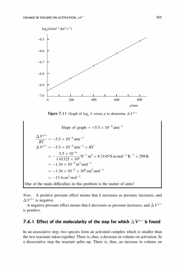
Slope of graph ¼ þ5:5 10�4 atm�1
�V 6¼ �
RT¼ �5:5 10�4 atm�1
�V 6¼ � ¼ �5:5 10�4 atm�1 RT
¼ � 5:5 10�4
1:01325 105N�1 m2 8:3145 N m mol�1 K�1 298 K
¼ �1:34 10�5 m3 mol�1
¼ �1:34 10�5 106 cm3 mol�1
¼ �13:4 cm3 mol�1
One of the main difficulties in this problem is the matter of units!
Note. A positive pressure effect means that k increases as pressure increases, and
�V 6¼ � is negative.
A negative pressure effect means that k decreases as pressure increases, and �V 6¼ �
is positive.
7.6.1 Effect of the molecularity of the step for which �V 6¼ � is found
In an associative step, two species form an activated complex which is smaller than
the two reactants taken together. There is, thus, a decrease in volume on activation. In
a dissociative step the reactant splits up. There is, thus, an increase in volume on
_6.5
_6.6
_6.7
_6.8
_6.9
_7.00 200 400 600 800
loge(k/mol_1 dm3 s
_1)
p/atm
Figure 7.11 Graph of loge k versus p to determine �V 6¼ �
CHANGE IN VOLUME ON ACTIVATION, �V 6¼* 305
activation. An interchange step gives intermediate changes, and the volume change is
expected to be fairly small.
7.6.2 Effect of complexity of structure
Change in the internal motions of rotations and vibrations will make a very minor
contribution. This contrasts with the much larger possible effect of a change in the
overall volume, which reflects major changes in size between the overall size of the
reactants and the activated complex.
7.6.3 Effect of charge on �V 6¼ � for reactions between ions
Equation (4.40) is the starting point, with the corresponding expression for reaction
between ions in solution being Equation (7.26).
�G6¼ �ions in solution ¼ �G
6¼ �molecules in gas þ
zA zB e2
4� "0 "r r6¼ð7:26Þ
But �G for reactions in solution depends on pressure, in contrast to gas phase
reactions, for which �G is independent of pressure.
One of the key equations of thermodynamics is
dG ¼ Vd p� Sd T ð7:39Þ
At constant T, d T ¼ 0, and S d T ¼ 0, giving
d G ¼ V d p ð7:40Þðp2
p1
d G ¼ðp2
p1
V d p ð7:41Þ
For an ideal gas
p V ¼ n RT ð7:42Þ
giving
ðp2
p1
d G ¼ n RT
ðp2
p1
d p
pð7:43Þ
from which
Gp2� Gp1
¼ n RT loge
p2
p1
ð7:44Þ
306 REACTIONS IN SOLUTION
and, if the standard state is 1 atm (more recently 1 bar¼ 1.000 00 105 N m�2),
then
� ¼ � þ RT loge p ð7:45Þ
where � is a constant dependent on T and independent of p. �G is a combination of
� values for products and reactants, and so is also independent of pressure.
For a substance in solution, the analogous equation for the ideal case is
� ¼ � þ RT loge c ð7:46Þ
where � is a constant dependent on T and also on pressure.
Correspondingly, �G is a constant dependent on both T and pressure.
This means that the comparison has to be with molecules in solution, rather than
molecules in the gas phase, as was appropriate for � S6¼ � and �H 6¼ �. The appropriate
starting equation is thus not (7.26), but
�G6¼ �ions in solution ¼ �G
6¼ �molecules in solution þ
zA zB e2
4� "0 "r r6¼ð7:47Þ
Since for reactions in solution
@�G
@ p
� �T
¼ þ�V ð4:36Þ
Equation (7.47) has to be differentiated with respect to pressure at constant
temperature. This requires a knowledge of the pressure dependence of the relative
permittivity at constant temperature.
The relative permittivity "r increases with increase in pressure. Thus for ions of like
charge (zA zB positive), the electrostatic term in Equation (7.47) decreases as p
increases. This gives a negative contribution to @�G 6¼ �=@ p �
T, and therefore a
negative contribution to �V 6¼ �. Consequently �V 6¼ � is predicted to be less than the
value it would have taken if there had been no electrostatic term.
For ions of unlike charge (zA zB negative), �V 6¼ � is predicted to be greater than the
value which it would have taken if there had been no electrostatic term.
This can be summarized as
for ions of like sign; �V6¼ �ions in solution < �V
6¼ �molecules in solution
for ions of unlike sign; �V6¼ �ions in solution > �V
6¼ �molecules in solution
and so �V6¼ �ions in solution for ions of like sign is likely to be less than �V
6¼ �ions in solution for
ions of unlike sign.
CHANGE IN VOLUME ON ACTIVATION, �V 6¼* 307
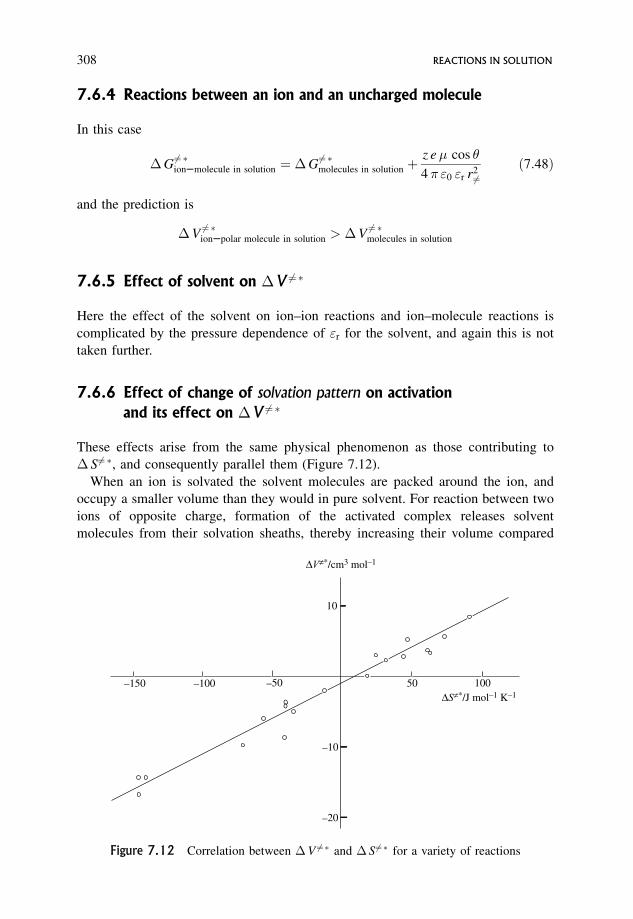
7.6.4 Reactions between an ion and an uncharged molecule
In this case
�G6¼ �ion--molecule in solution ¼ �G
6¼ �molecules in solution þ
z e� cos
4� "0 "r r26¼
ð7:48Þ
and the prediction is
�V6¼ �ion--polar molecule in solution > �V
6¼ �molecules in solution
7.6.5 Effect of solvent on �V 6¼ �
Here the effect of the solvent on ion–ion reactions and ion–molecule reactions is
complicated by the pressure dependence of "r for the solvent, and again this is not
taken further.
7.6.6 Effect of change of solvation pattern on activation
and its effect on �V 6¼ �
These effects arise from the same physical phenomenon as those contributing to
� S6¼ �, and consequently parallel them (Figure 7.12).
When an ion is solvated the solvent molecules are packed around the ion, and
occupy a smaller volume than they would in pure solvent. For reaction between two
ions of opposite charge, formation of the activated complex releases solvent
molecules from their solvation sheaths, thereby increasing their volume compared
50_50_100_150 100
10
_10
_20
∆V≠*/cm3 mol_1
∆S≠*/J mol_1 K
_1
Figure 7.12 Correlation between �V 6¼ � and � S 6¼ � for a variety of reactions
308 REACTIONS IN SOLUTION
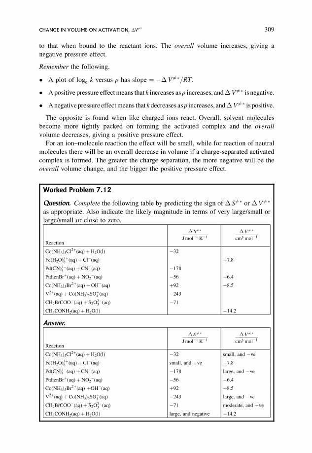
to that when bound to the reactant ions. The overall volume increases, giving a
negative pressure effect.
Remember the following.
� A plot of loge k versus p has slope ¼ ��V 6¼ �=RT .
� A positive pressure effect means that k increases as p increases, and�V 6¼ � is negative.
� A negative pressure effect means that k decreases as p increases, and�V 6¼ � is positive.
The opposite is found when like charged ions react. Overall, solvent molecules
become more tightly packed on forming the activated complex and the overall
volume decreases, giving a positive pressure effect.
For an ion–molecule reaction the effect will be small, while for reaction of neutral
molecules there will be an overall decrease in volume if a charge-separated activated
complex is formed. The greater the charge separation, the more negative will be the
overall volume change, and the bigger the positive pressure effect.
Worked Problem 7.12
Question. Complete the following table by predicting the sign of � S6¼ � or �V 6¼ �
as appropriate. Also indicate the likely magnitude in terms of very large/small or
large/small or close to zero.
Reaction
� S6¼ �
J mol�1 K�1
�V 6¼ �
cm3 mol�1
Co(NH3)5Cl2þ(aq)þH2O(l) �32
Fe(H2O)3þ6 (aq)þ Cl�(aq) þ7.8
Pd(CN)2�4 (aq)þ CN�(aq) �178
PtdienBrþ(aq)þNO2�(aq) �56 �6.4
Co(NH3)5Br2þ(aq)þOH�(aq) þ92 þ8.5
V2þ(aq)þ Co(NH3)5SOþ4 (aq) �243
CH2BrCOO�(aq)þ S2O2�3 (aq) �71
CH3CONH2(aq)þH2O(l) �14.2
Answer.
Reaction
� S 6¼ �
J mol�1 K�1
�V 6¼ �
cm3 mol�1
Co(NH3)5Cl2þ(aq)þH2O(l) �32 small, and �ve
Fe(H2O)3þ6 (aq)þ Cl�(aq) small, and þve þ7.8
Pd(CN)2�4 (aq)þ CN�(aq) �178 large, and �ve
PtdienBrþ(aq)þNO2�(aq) �56 �6.4
Co(NH3)5Br2þ(aq) þOH�(aq) þ92 þ8.5
V2þ(aq)þ Co(NH3)5SOþ4 (aq) �243 large, and �ve
CH2BrCOO�(aq)þ S2O2�3 (aq) �71 moderate, and �ve
CH3CONH2(aq)þH2O(l) large, and negative �14.2
CHANGE IN VOLUME ON ACTIVATION, �V 6¼* 309
7.7 Terms Contributing to Activation Parameters
7.7.1 � S 6¼ �
� Is the step associative or dissociative or neither?
Associative, i.e. 2! 1: expect a loss in entropy; � S6¼ � is �ve.
Dissociative, i.e. 1! 2: expect a gain in entropy; � S6¼ � is þve.
Interchange: expect a small change in entropy, i.e. � S6¼ � is close to zero.
Remember to distinguish between the mechanism and the individual steps in it.
� Change in internal modes for large species
Expect a loss in entropy. � S 6¼ � is �ve.
� Effect of charges: electrostatic term involving charge and solvent
1. Like charges: expect a loss of entropy. � S6¼ � is �ve.
2. Unlike charges: expect a gain in entropy. � S6¼ � is þve.
3. Ion–molecule: expect a small increase in entropy. � S6¼ � is slightly þve.
4. Molecule–molecule with a charge-separated activated complex: expect a
decrease. � S6¼ � is slightly �ve.
5. Molecule–molecule without charge separation in the activated complex: expect
a small increase or decrease. � S6¼ � is slightly þve or �ve.
� Change in solvation pattern on forming the activated complex
1. Like charges: expect a loss of entropy. � S6¼ � is �ve.
2. Unlike charges: expect a gain in entropy. � S6¼ � is þve.
3. Ion–molecule: expect either a small loss or gain in entropy. � S6¼ � is slightly
þve or �ve.
4 and 5. Molecule–molecule: expect a loss in entropy though it could be small.
� S6¼ � is slightly �ve.
But, what is the basis of comparison; i.e., is the typical gas phase value to be used,
and, if not, what value?
7.7.2 �V 6¼ �
� Is the step associative or dissociative or neither?
Associative, i.e. 2! 1: expect a decrease in volume; �V 6¼ � is �ve.
Dissociative, i.e 1! 2: expect an increase in volume; �V 6¼ � is þve.
Interchange: expect a small change in volume, i.e. �V 6¼ � is close to zero.
310 REACTIONS IN SOLUTION
� Change in internal modes for large species
does not enter into the volume of activation. This makes the interpretation of
volumes of activation more straightforward than that for entropies of activation.
� Effect of charges: electrostatic term involving charge and solvent
1. Like charges: expect a decrease of volume; �V 6¼ � is �ve.
2. Unlike charges: expect an increase in volume; �V 6¼ � is þve.
3. Ion–molecule: expect an increase in volume; �V 6¼ � is þve.
4. Molecule–molecule with a charged-separated activated complex: expect a
decrease in volume; �V 6¼ � is �ve.
5. Molecule–molecule without charge separation in the activated complex: expect
a small decrease in volume; �V 6¼ � is slightly �ve.
� Change in solvation pattern on forming the activated complex
1. Like charges: expect a decrease in volume; �V 6¼ � is �ve.
2. Unlike charges: expect an increase in volume; �V 6¼ � is þve.
3. Ion–molecule: expect either a small increase or decrease in volume; �V 6¼ � is
slightly þve or �ve.
4. Molecule–molecule: expect a decrease in volume, though it could be small;
�V 6¼ � is slightly �ve.
But, again, what value should be taken as the basis of comparison?
7.7.3 �H6¼ �
� Is the step associative or dissociative or neither?
Associative, i.e. 2! 1: bond formation – expect a lower value of �H 6¼ �.Dissociative, i.e. 1! 2: bond breaking – expect a higher value of �H 6¼ �.Interchange: expect �H 6¼ � to take intermediate values.
Change of internal modes for a large species
Does not enter into the enthalpy of activation; this makes for a more straightfor-
ward interpretation of enthalpies of activation than entropies of activation.
� Effect of charges: electrostatic term involving charge and solvent
1. Like charges: expect a smaller value for �H 6¼ �.
TERMS CONTRIBUTING TO ACTIVATION PARAMETERS 311
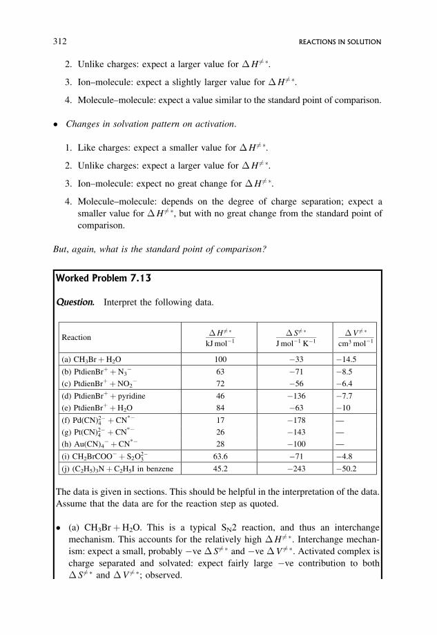
2. Unlike charges: expect a larger value for �H 6¼ �.
3. Ion–molecule: expect a slightly larger value for �H 6¼ �.
4. Molecule–molecule: expect a value similar to the standard point of comparison.
� Changes in solvation pattern on activation.
1. Like charges: expect a smaller value for �H 6¼ �.
2. Unlike charges: expect a larger value for �H 6¼ �.
3. Ion–molecule: expect no great change for �H 6¼ �.
4. Molecule–molecule: depends on the degree of charge separation; expect a
smaller value for �H 6¼ �, but with no great change from the standard point of
comparison.
But, again, what is the standard point of comparison?
Worked Problem 7.13
Question. Interpret the following data.
Reaction�H 6¼ �
kJ mol�1
� S6¼ �
J mol�1 K�1
�V 6¼ �
cm3 mol�1
(a) CH3BrþH2O 100 �33 �14.5
(b) PtdienBrþ þN3� 63 �71 �8.5
(c) PtdienBrþ þNO2� 72 �56 �6.4
(d) PtdienBrþ þ pyridine 46 �136 �7.7
(e) PtdienBrþ þH2O 84 �63 �10
(f) Pd(CN)2�4 þ CN*� 17 �178 —
(g) Pt(CN)2�4 þ CN*� 26 �143 —
(h) Au(CN)4� þ CN*� 28 �100 —
(i) CH2BrCOO� þ S2O2�3 63.6 �71 �4.8
(j) (C2H5)3Nþ C2H5I in benzene 45.2 �243 �50.2
The data is given in sections. This should be helpful in the interpretation of the data.
Assume that the data are for the reaction step as quoted.
� (a) CH3BrþH2O. This is a typical SN2 reaction, and thus an interchange
mechanism. This accounts for the relatively high �H 6¼ �. Interchange mechan-
ism: expect a small, probably �ve � S6¼ � and �ve �V 6¼ �. Activated complex is
charge separated and solvated: expect fairly large �ve contribution to both
� S 6¼ � and �V 6¼ �; observed.
312 REACTIONS IN SOLUTION
� (b) PtdienBrþ þN�3 and (c) PtdienBrþ þNO�2 . �H 6¼ � suggests an interchange
mechanism, but the values are low enough to correspond to interchange with
associative characteristics. Expect a �ve � S6¼ � and �ve �V 6¼ �. But reaction is
(þ1) with (�1) charge, which should give a þve contribution to both, because of
the charge and solvation effects. The complexity of the dien would give a �ve
contribution to � S 6¼ �. Overall a fairly small � S6¼ � and �V 6¼ � is reasonable, as
observed.
� (d) PtdienBrþ þ pyridine and (e) PtdienBrþ þH2O. �H 6¼ � values again sug-
gest an interchange mechanism with associative characteristics. The � S6¼ � and
�V 6¼ � values for (e), i.e. reaction with H2O, are in line with those of reactions
(b) and (c), even though this is an ionþ dipole reaction, where the charge and
solvation effects will make a less þve contribution than for reactions (b) and (c).
Reaction (d) i.e. with pyridine, has a surprisingly large �ve � S6¼ �, but a
�V 6¼ � in keeping with those for reactions (b) and (c). Perhaps the high
polarizability of the pyridine might lead it to be held relatively rigidly in the
activated complex, causing a substantial �ve � S6¼ � contribution. This would be
reinforced by a contribution from the relative complexity of pyridine compared
with water. Neither factor would affect the �V 6¼ �.
� (f), (g) and (h), i.e. Pd(CN)2�4 þ C*N�, Pt(CN)2�
4 þ C*N� and Au(CN)�4 þC*N�. All have small �H 6¼ � values indicative of an associative mechanism.
Reactions (f) and (g) are (�2) with (�1) charge reactions, and a large �ve
contribution to � S6¼ � from the effect of charge and solvation would be expected.
This would be reinforced by any �ve contribution from the complexity of the
complexes.
This can be contrasted with reaction (h), which has a less �ve � S6¼ � value,
but this would be expected since the activated complex would have a �2 charge
compared to �3 for reactions (f) and (g). This would lead to a less �ve
contribution to � S6¼ � from the charge and solvation effects.
� (i) CH2BrCOO� þ S2O2�3 . The �H 6¼ � value suggests an interchange mechan-
ism in keeping with the SN2 characteristics of the substitution of S2O2�3 for Br�.
The � S 6¼ � and �V 6¼ � values are relatively small and �ve, supporting the
inference that this is an interchange rather an associative mechanism. Because of
the charges, (�1) with (�2), there would be a fairly large �ve contribution to
� S6¼ � and �V 6¼ �.
� ( j) (C2H5)3Nþ C2H5I in benzene. This reaction produces a quaternary ammo-
nium salt, which would be fully associated in benzene. It would, however, be
charge separated. The very large �ve values for both � S6¼ � and �V 6¼ � suggest
that there is a considerable degree of charge separation in the activated complex,
and that this is an associative mechanism. This would be reinforced by a
contribution due to the complexity of both reactants. The fairly low value of
�H 6¼ � supports an associative mechanism.
TERMS CONTRIBUTING TO ACTIVATION PARAMETERS 313
Further reading
Laidler K.J., Chemical Kinetics, 3rd edn, Harper and Row, New York, 1987.
Laidler K.J. and Meiser J.H., Physical Chemistry, 3rd edn, Houghton Mifflin, New
York, 1999.
Alberty R.A. and Silbey R.J., Physical Chemistry, 2nd edn, Wiley, New York, 1996.
Logan S.R., Fundamentals of Chemical Kinetics, Addison-Wesley, Reading, MA,
1996.
*Wilkinson F., Chemical Kinetics and Reaction Mechanisms, Van Nostrand Reinhold,
New York, 1980.
Robson Wright M., Fundamental Chemical Kinetics, Horwood, Chichester, 1999.
*Laidler K.J., Theories of Chemical Reaction Rates, McGraw-Hill, New York,
1969.
*Glasstone S., Laidler K.J. and Eyring H., Theory of Rate Processes, McGraw-Hill,
New York, 1941.
*Robson Wright M., Nature of Electrolyte Solutions, Macmillan, Basingstoke,
1988.
Robson Wright M., Behaviour and Nature of Electrolyte Solutions, Wiley, Chichester,
in preparation.
Hay R.W., Reaction Mechanisms of Metal Complexes, Horwood, Chichester,
2000.
Cox B.G., Modern Liquid Phase Kinetics, Oxford University Press, Oxford, 1994.
Wilkins R.G., Kinetics and Mechanisms of Transition Metal Complexes, Verlagsges-
selchaft, Cambridge, 1999.
Burgess J. and Tobe M., Inorganic Reaction Mechanisms, Longman, London,
2000.*Out of print, but should be available in university libraries.
Further problems
1. When SO2�4 is added to the reaction mixture for the acid-catalysed hydrolysis of
acetylcholine, (CH3)3NþCH2CH2OCOCH3 (HEþ), with H3Oþ, added catalysis is
observed. This can be interpreted as anion-catalysed hydrolysis by SO2�4 , or as
general acid catalysis by HSO�4 . Predict the effect of ionic strength on the rate
constants describing each mechanism, and comment on the result. Does this
represent a means of distinguishing between the two mechanisms?
2. The following observations relate to an investigation of the reaction
CH2ClCOO�ðaqÞ þ OH�ðaqÞ ! CH2OHCOO�ðaqÞ þ Cl�ðaqÞ
314 REACTIONS IN SOLUTION
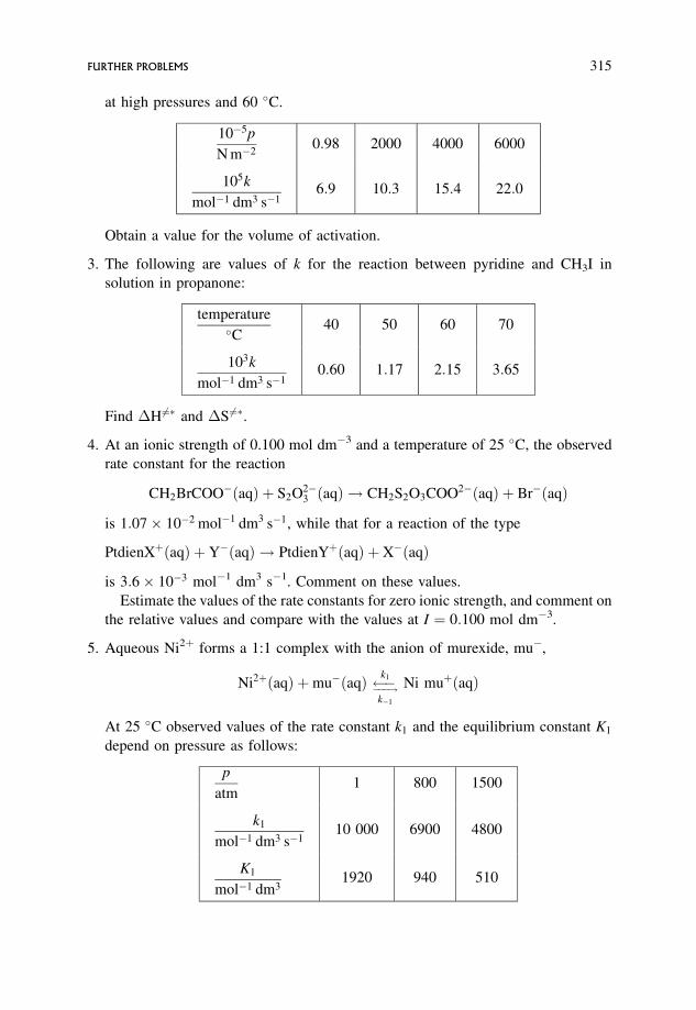
at high pressures and 60 �C.
10�5p
N m�20:98 2000 4000 6000
105k
mol�1 dm3 s�16:9 10:3 15:4 22:0
Obtain a value for the volume of activation.
3. The following are values of k for the reaction between pyridine and CH3I in
solution in propanone:
temperature�C
40 50 60 70
103k
mol�1 dm3 s�10:60 1:17 2:15 3:65
Find �H6¼� and �S 6¼�.
4. At an ionic strength of 0.100 mol dm�3 and a temperature of 25 �C, the observed
rate constant for the reaction
CH2BrCOO�ðaqÞ þ S2O2�3 ðaqÞ ! CH2S2O3COO2�ðaqÞ þ Br�ðaqÞ
is 1:07 10�2 mol�1 dm3 s�1, while that for a reaction of the type
PtdienXþðaqÞ þ Y�ðaqÞ ! PtdienYþðaqÞ þ X�ðaqÞ
is 3:6 10�3 mol�1 dm3 s�1. Comment on these values.
Estimate the values of the rate constants for zero ionic strength, and comment on
the relative values and compare with the values at I ¼ 0:100 mol dm�3.
5. Aqueous Ni2þ forms a 1:1 complex with the anion of murexide, mu�,
Ni2þðaqÞ þmu�ðaqÞ ����!k1
k�1
Ni muþðaqÞ
At 25 �C observed values of the rate constant k1 and the equilibrium constant K1
depend on pressure as follows:
p
atm1 800 1500
k1
mol�1 dm3 s�110 000 6900 4800
K1
mol�1 dm31920 940 510
FURTHER PROBLEMS 315
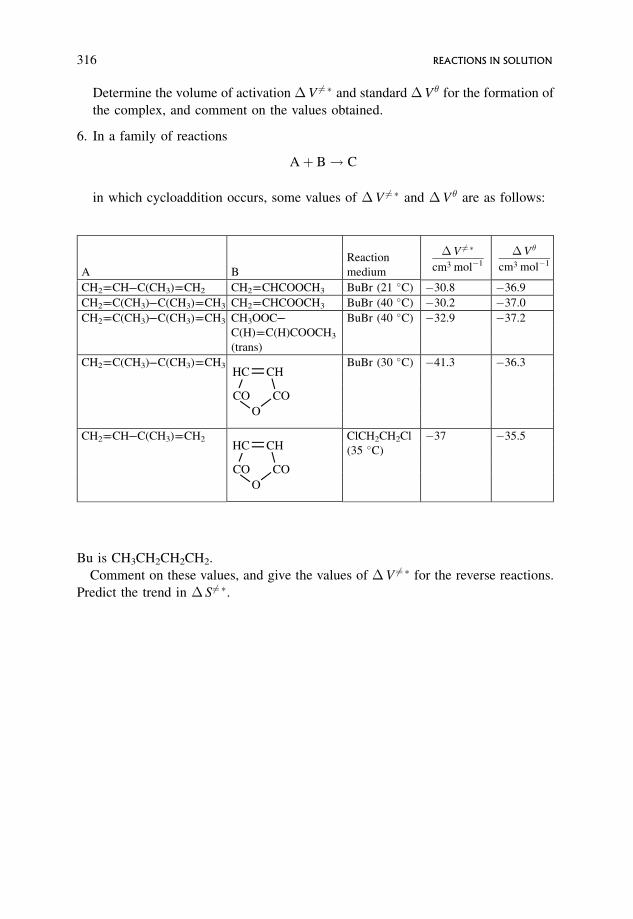
Determine the volume of activation �V 6¼ � and standard �V for the formation of
the complex, and comment on the values obtained.
6. In a family of reactions
Aþ B! C
in which cycloaddition occurs, some values of �V 6¼ � and �V are as follows:
Bu is CH3CH2CH2CH2.
Comment on these values, and give the values of �V 6¼ � for the reverse reactions.
Predict the trend in � S6¼ �.
A B
Reaction
medium
�V 6¼ �
cm3 mol�1
�V
cm3 mol�1
CH2����CH��C(CH3)����CH2 CH2����CHCOOCH3 BuBr (21 �C) �30.8 �36.9
CH2����C(CH3)��C(CH3)����CH3 CH2����CHCOOCH3 BuBr (40 �C) �30.2 �37.0
CH2����C(CH3)��C(CH3)����CH3 CH3OOC��C(H)����C(H)COOCH3
(trans)
BuBr (40 �C) �32.9 �37.2
CH2����C(CH3)��C(CH3)����CH3
CO
CHHC
COO
BuBr (30 �C) �41.3 �36.3
CH2����CH��C(CH3)����CH2
CO
CHHC
COO
ClCH2CH2Cl
(35 �C)
�37 �35.5
316 REACTIONS IN SOLUTION
8 Examples of Reactions
in Solution
This chapter applies many of the techniques discussed in previous chapters to the
determination of rate constants for complex reactions in solution. It also focuses on a
variety of types of reaction in solution.
Aims
By the end of this chapter you should be able to
� solve problems on reactions with two contributions to the overall rate
� solve problems on reactions with concurrent routes, where both reactants are inequilibrium
� recognize kinetically equivalent mechanisms
� handle metal ion and anion catalysis
� recognize and handle mechanisms involving pre-equilibria and
� handle steady state situations for reactions with an initial reversible step
8.1 Reactions Where More than One Reaction Contributes
to the Rate of Removal of Reactant
This section will discuss reaction mechanisms of ever-increasing complexity.
An Introduction to Chemical Kinetics. Margaret Robson Wright# 2004 John Wiley & Sons, Ltd. ISBNs: 0-470-09058-8 (hbk) 0-470-09059-6 (pbk)
8.1.1 A simple case
Reactions in solution often have a contribution to the overall rate from reaction of the
solvent with one or other of the reactants; e.g., hydrolyses of esters in aqueous
solution often have a contribution from a ‘water’ rate.
A typical base hydrolysis may have two contributing reactions:
esterðaqÞ þ OH�ðaqÞ�!k1products
esterðaqÞ þ H2OðlÞ�!k2products
where the products are the carboxylate ion and an alcohol.
Mechanistic rate:
� d½ester�dt
¼ k1½ester�½OH�� þ k2½ester� ð8:1Þ
where the rate of the second reaction does not include [H2O], since this is in
considerable excess and remains virtually constant throughout the reaction. k2 is thus
a pseudo-first order rate constant, with units time�1.
Observed rate:
� d½ester�dt
¼ kobs½ester�½OH�� ð8:2Þ
If the mechanism is correct, then
kobs½ester�½OH�� ¼ k1½ester�½OH�� þ k2½ester� ð8:3Þ
giving
kobs ¼ k1 þ k2=½OH�� ð8:4Þ
Experimental rate constants gathered for experiments over a range of [OH�]
should determine whether there is a ‘water’ rate or not, and allow k1 and/or k2 to be
found.
If there is no water rate, then kobs values will be independent of [OH�]. If kobs does
depend on [OH�], then a graph of kobs versus 1/[OH�] should be linear, with
slope¼ k2 and intercept¼ k1.
A very common problem in kinetics
kobs ¼ k1 þ k2=½OH�� ð8:4Þ
The method of analysis implies that kobs is found at various [OH�]. But there is a
problem – OH� is used up during each experiment. How can this be overcome?
318 EXAMPLES OF REACTIONS IN SOLUTION
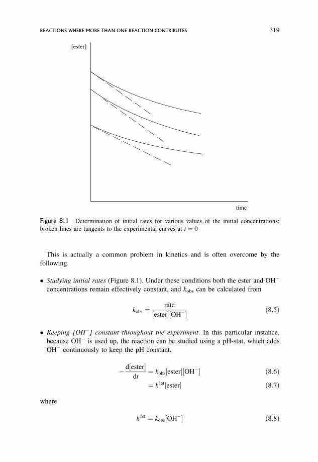
This is actually a common problem in kinetics and is often overcome by the
following.
� Studying initial rates (Figure 8.1). Under these conditions both the ester and OH�
concentrations remain effectively constant, and kobs can be calculated from
kobs ¼rate
½ester�½OH�� ð8:5Þ
� Keeping [OH�] constant throughout the experiment. In this particular instance,
because OH� is used up, the reaction can be studied using a pH-stat, which adds
OH� continuously to keep the pH constant.
� d½ester�dt
¼ kobs½ester�½OH�� ð8:6Þ
¼ k1st½ester� ð8:7Þ
where
k1st ¼ kobs½OH�� ð8:8Þ
time
[ester]
Figure 8.1 Determination of initial rates for various values of the initial concentrations:
broken lines are tangents to the experimental curves at t ¼ 0
REACTIONS WHERE MORE THAN ONE REACTION CONTRIBUTES 319
The volume of OH� added gives a measure of how much ester has been hydrolysed at
various times throughout the reaction, and enables the pseudo-first order rate constant
k1st to be found, from which the second order kobs can be calculated.
The following problem illustrates the analysis given above.
Worked Problem 8.1
Question. The following kinetic data have been obtained for the reaction of
pyridine with Pt(dien)Clþ, where dien has the structure NH2(CH2)2NH(CH2)2NH2,
½PtðdienÞCl�þðaqÞ þ pyridineðaqÞ ! ½PtðdienÞpyridine�2þðaqÞ þ Cl�ðaqÞ
The concentration of the complex was 1:00 10�3 mol dm�3 in each experiment.
½pyridine�mol dm�3 0:100 0:200 0:300 0:400 0:500
103kobs
s�11:75 2:70 3:65 4:60 5:55
� What can be said about the relative concentrations of pyridine and complex, and
what does this imply for the conditions of the experiment? What does this imply
about the observed rate constant and its units?
� Write down the steps involved in the reaction, and formulate an expression for
the mechanistic rate.
� Formulate the expression for the observed rate.
� Calculate (a) the first order rate constant for the reaction of the complex with the
solvent, water, (b) the pseudo-first order rate constant for reaction with pyridine
and (c) the second order rate constant for reaction with pyridine.
Answer. In all of the experiments [pyridine]� [complex]. Thus throughout each
experiment [pyridine] is being held effectively constant, and each experiment is
under pseudo-first order conditions, verified by the units of the observed rate
constant, s�1.
The two contributions to the overall reaction are
½PtðdienÞCl�þðaqÞ þ pyridineðaqÞ�!k1 ½PtðdienÞ pyridine�2þðaqÞ þ Cl�ðaqÞ
½PtðdienÞCl�þðaqÞ þ H2OðlÞ�!k2 ½PtðdienÞH2O�2þðaqÞ þ Cl�ðaqÞ
Mechanistic rate:
� d½Pt dienð ÞCl�þ
dt¼ k1½PtðdienÞClþ�½pyridine� þ k2½PtðdienÞClþ� ð8:9Þ
320 EXAMPLES OF REACTIONS IN SOLUTION
Observed rate ¼ k2ndobs ½PtðdienÞClþ�½pyridine� ð8:10Þ
¼ k1stobs½PtðdienÞClþ� ð8:11Þ
where k2ndobs is a second order rate constant, k1st
obs is a pseudo-first order rate constant
and
k1stobs ¼ k2nd
obs ½pyridine� ð8:12Þ
If the mechanism is correct, then
k1stobs½PtðdienÞClþ� ¼ k1½PtðdienÞClþ�½pyridine� þ k2½PtðdienÞClþ� ð8:13Þ
k1stobs ¼ k1½pyridine� þ k2 ð8:14Þ
A plot of k1stobs versus [pyridine] should be linear with slope¼ k1 and intercept¼ k2.
If there is no contribution from the reaction of the complex with water, then the
graph will go through the origin, and k2 will be zero.
From the data given, the graph of k1stobs versus [pyridine] is linear with a non-zero
intercept (Figure 8.2), with
slope ¼ 9:5 10�3 mol�1 dm3 s�1 giving k1 ¼ 9:5 10�3 mol�1 dm3 s�1
intercept ¼ 0:80 10�3 s�1 giving k2 ¼ 8:0 10�4 s�1
8.1.2 A slightly more complex reaction where reaction occurs by
two concurrent routes, and where both reactants are in
equilibrium with each other
In the specific example chosen here the analysis is made easier because of
approximations which can be made as a result of the magnitude of the equilibrium
constant. This is not always the case (Section 8.2.2).
The base hydrolysis of aminoacid esters
This can be illustrated by the hydrolysis of a simple aminoacid ester. Glycine ethyl
ester exists as
the unprotonated ester; E; NH2CH2COOCH2CH3
the protonated ester;HEþ; NHþ3 CH2COOCH2CH3
REACTIONS WHERE MORE THAN ONE REACTION CONTRIBUTES 321
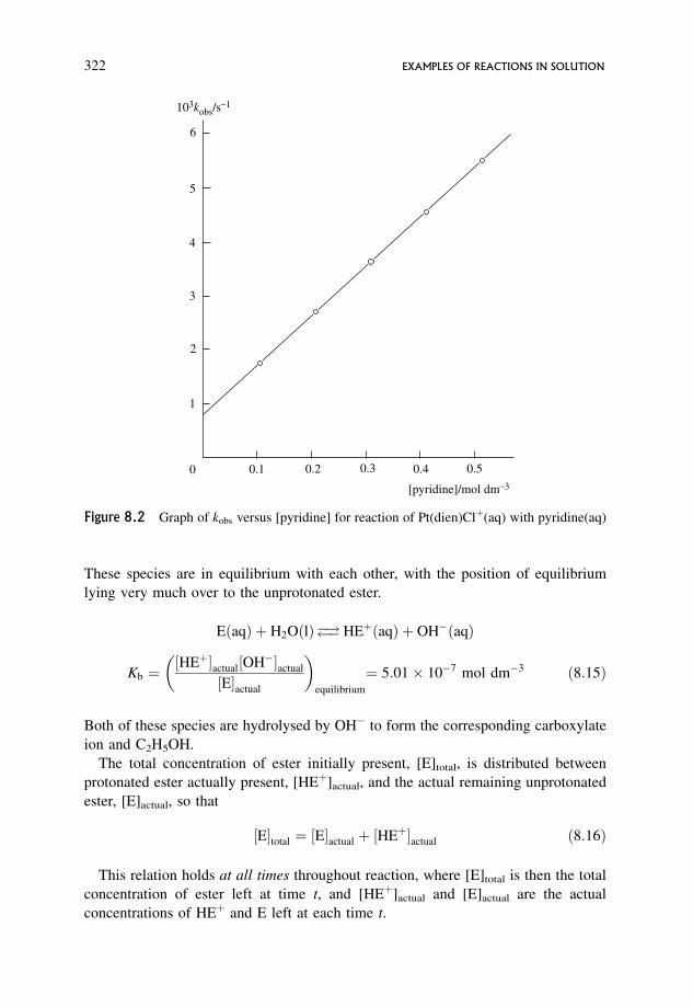
These species are in equilibrium with each other, with the position of equilibrium
lying very much over to the unprotonated ester.
EðaqÞ þ H2OðlÞ�! � HEþðaqÞ þ OH�ðaqÞ
Kb ¼½HEþ�actual½OH��actual
½E�actual
� �equilibrium
¼ 5:01 10�7 mol dm�3 ð8:15Þ
Both of these species are hydrolysed by OH� to form the corresponding carboxylate
ion and C2H5OH.
The total concentration of ester initially present, [E]total, is distributed between
protonated ester actually present, [HEþ]actual, and the actual remaining unprotonated
ester, [E]actual, so that
½E�total ¼ ½E�actual þ ½HEþ�actual ð8:16Þ
This relation holds at all times throughout reaction, where [E]total is then the total
concentration of ester left at time t, and [HEþ]actual and [E]actual are the actual
concentrations of HEþ and E left at each time t.
0
1
2
3
4
5
6
0.1 0.2 0.3 0.4 0.5
[pyridine]/mol dm_3
103kobs/s_1
Figure 8.2 Graph of kobs versus [pyridine] for reaction of Pt(dien)Clþ(aq) with pyridine(aq)
322 EXAMPLES OF REACTIONS IN SOLUTION
Reaction is first order in ester for experiments at constant pH, and further
experiments at other constant pH values show reaction to be first order in OH�.
The reaction can be followed very conveniently using a pH-stat, so that [OH�] is
kept constant throughout reaction by continuous addition of OH�. The volume of
OH� added at various times enables the total amount of ester hydrolysed at these
times to be found.
The observed rate is defined in terms of the total amount of ester used up, without
reference to the two forms of the ester. But the mechanism ‘is interested’ in the
chemical steps involved in the reaction, and this must refer to the hydrolysis of both
forms of the ester:
Eþ OH� �!k1products
HEþ þ OH� �!k2products
and both steps contribute to the predicted overall rate of removal of ester.
Mechanistic rate
� d½E�total
dt¼ k1½E�actual½OH��actual þ k2½HEþ�actual½OH��actual ð8:17Þ
where [E]total, [E]actual and [HEþ]actual vary throughout the experiment, and will be
the instantaneous values at the times at which the rate is measured (Figure 8.3).
Observed rate
This is measured in terms of the total ester used up at any given time:
� d½E�total
dt¼ kobs½E�total½OH��actual ð8:18Þ
If the proposed mechanism is correct, then these rates must be equal.
kobs½E�total½OH��actual ¼ k1½E�actual½OH��actual þ k2½HEþ�actual½OH��actual ð8:19Þ
kobs½E�total ¼ k1½E�actual þ k2½HEþ�actual ð8:20Þ
kobs ¼ k1
½E�actual
½E�total
þ k2
½HEþ�actual
½E�total
ð8:21Þ
All of the concentration terms are related to each other, so this equation can be
simplified. Equation (8.15) rearranged gives
½HEþ�actual ¼Kb½E�actual
½OH��actual
ð8:22Þ
REACTIONS WHERE MORE THAN ONE REACTION CONTRIBUTES 323
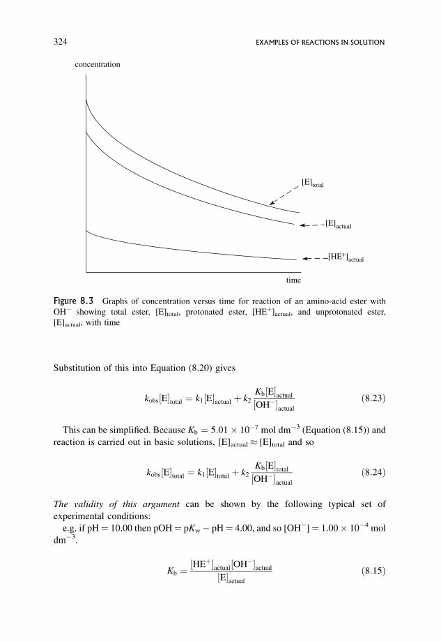
Substitution of this into Equation (8.20) gives
kobs½E�total ¼ k1½E�actual þ k2
Kb½E�actual
½OH��actual
ð8:23Þ
This can be simplified. Because Kb ¼ 5:01 10�7 mol dm�3 (Equation (8.15)) and
reaction is carried out in basic solutions, [E]actual [E]total and so
kobs½E�total ¼ k1½E�total þ k2
Kb½E�total
½OH��actual
ð8:24Þ
The validity of this argument can be shown by the following typical set of
experimental conditions:
e.g. if pH¼ 10.00 then pOH¼ pKw� pH¼ 4.00, and so [OH�]¼ 1.00 10�4 mol
dm�3.
Kb ¼½HEþ�actual½OH��actual
½E�actual
ð8:15Þ
[E]actual
[E]total
[HE+]actual
time
concentration
Figure 8.3 Graphs of concentration versus time for reaction of an amino-acid ester with
OH� showing total ester, [E]total, protonated ester, [HEþ]actual, and unprotonated ester,
[E]actual, with time
324 EXAMPLES OF REACTIONS IN SOLUTION
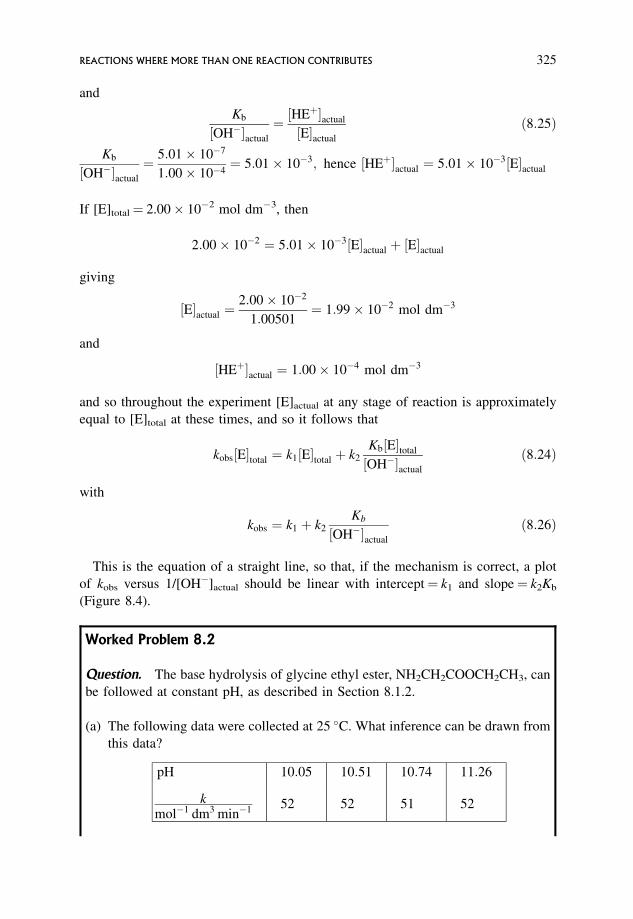
and
Kb
½OH��actual
¼ ½HEþ�actual
½E�actual
ð8:25Þ
Kb
½OH��actual
¼ 5:01 10�7
1:00 10�4¼ 5:01 10�3; hence ½HEþ�actual ¼ 5:01 10�3½E�actual
If [E]total¼ 2.00 10�2 mol dm�3, then
2:00 10�2 ¼ 5:01 10�3½E�actual þ ½E�actual
giving
½E�actual ¼2:00 10�2
1:00501¼ 1:99 10�2 mol dm�3
and
½HEþ�actual ¼ 1:00 10�4 mol dm�3
and so throughout the experiment [E]actual at any stage of reaction is approximately
equal to [E]total at these times, and so it follows that
kobs½E�total ¼ k1½E�total þ k2
Kb½E�total
½OH��actual
ð8:24Þ
with
kobs ¼ k1 þ k2
Kb
½OH��actual
ð8:26Þ
This is the equation of a straight line, so that, if the mechanism is correct, a plot
of kobs versus 1/[OH�]actual should be linear with intercept¼ k1 and slope¼ k2Kb
(Figure 8.4).
Worked Problem 8.2
Question. The base hydrolysis of glycine ethyl ester, NH2CH2COOCH2CH3, can
be followed at constant pH, as described in Section 8.1.2.
(a) The following data were collected at 25 �C. What inference can be drawn from
this data?
pH 10:05 10:51 10:74 11:26
kmol�1 dm3 min�1 52 52 51 52
REACTIONS WHERE MORE THAN ONE REACTION CONTRIBUTES 325
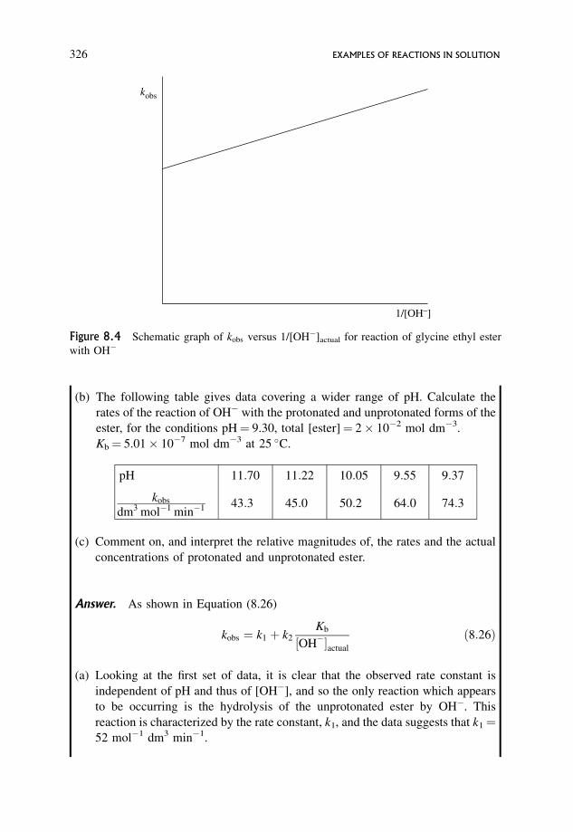
(b) The following table gives data covering a wider range of pH. Calculate the
rates of the reaction of OH� with the protonated and unprotonated forms of the
ester, for the conditions pH¼ 9.30, total [ester]¼ 2 10�2 mol dm�3.
Kb¼ 5.01 10�7 mol dm�3 at 25 �C.
pH 11:70 11:22 10:05 9:55 9:37
kobs
dm3 mol�1 min�1 43:3 45:0 50:2 64:0 74:3
(c) Comment on, and interpret the relative magnitudes of, the rates and the actual
concentrations of protonated and unprotonated ester.
Answer. As shown in Equation (8.26)
kobs ¼ k1 þ k2
Kb
½OH��actual
ð8:26Þ
(a) Looking at the first set of data, it is clear that the observed rate constant is
independent of pH and thus of [OH�], and so the only reaction which appears
to be occurring is the hydrolysis of the unprotonated ester by OH�. This
reaction is characterized by the rate constant, k1, and the data suggests that k1¼52 mol�1 dm3 min�1.
1/[OH_]
kobs
Figure 8.4 Schematic graph of kobs versus 1/[OH�]actual for reaction of glycine ethyl ester
with OH�
326 EXAMPLES OF REACTIONS IN SOLUTION
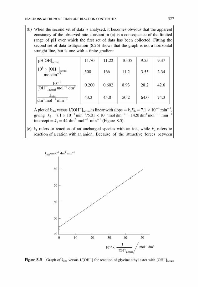
(b) When the second set of data is analysed, it becomes obvious that the apparent
constancy of the observed rate constant in (a) is a consequence of the limited
range of pH over which the first set of data has been collected. Fitting the
second set of data to Equation (8.26) shows that the graph is not a horizontal
straight line, but is one with a finite gradient
pH½OH�actual 11:70 11:22 10:05 9:55 9:37
105 ½OH��actual
mol dm�3 500 166 11:2 3:55 2:34
10�3
½OH��actual mol�1 dm3 0:200 0:602 8:93 28:2 42:6
kobs
dm3 mol�1 min�1 43:3 45:0 50:2 64:0 74:3
A plot of kobs versus 1/[OH�]actual is linear with slope¼ k2Kb¼ 7.1 10�4 min�1,
giving k2¼ 7.1 10�4 min�1/5.01 10�7mol dm�3¼ 1420 dm3 mol�1 min�1
intercept¼ k1¼ 44 dm3 mol�1 min�1 (Figure 8.5).
(c) k1 refers to reaction of an uncharged species with an ion, while k2 refers to
reaction of a cation with an anion. Because of the attractive forces between
10040
50
60
70
80
kobs/mol_1 dm3 min
_1
20 30 40 50
10_3 ×
[OH_]actual
mol_1 dm3 1
Figure 8.5 Graph of kobs versus 1/[OH�] for reaction of glycine ethyl ester with [OH�]actual
REACTIONS WHERE MORE THAN ONE REACTION CONTRIBUTES 327
oppositely charged ions, the rate constant for such a reaction will be much
higher than that for reaction between an ion and an uncharged molecule. The
observed values are in keeping with this qualitative prediction.
At pH¼ 9.30, since pHþ pOH¼ 14 then [OH�]¼ 2 10�5 mol dm�3;
[E]total [E]actual¼ 2 10�2 mol dm�3
½HEþ�actual ¼Kb½E�actual
½OH��actual
¼ 5:01 10�7 mol dm�3 2 10�2 mol dm�3
2 10�5 mol dm�3
¼ 5:01 10�4 mol dm�3
For the reaction EþOH� �!k1
rate ¼ k1½E�½OH��actual
¼ 44 dm3 mol�1 min�1 2 10�2 mol dm�3 2 10�5 mol dm�3
¼ 1:76 10�5 dm�3 mol min�1 ð8:27Þ
For the reaction HEþ þOH� �!k2
rate ¼ k2½HEþ�½OH��actual
¼ 1420 dm3 mol�1 min�1 5:01 10�4 mol dm�3 2 10�5 mol dm�3
¼ 1:42 10�5 dm�3 mol min�1 ð8:28Þ
Although [HEþ]� [E], the contributions to the overall rate from the protonated
and unprotonated ester hydrolyses are approximately equal. This is because
k2� k1. A very small concentration combined with a large rate constant can still
make a significant contribution to the rate.
An important point. The other important conclusion to be drawn from this
problem is the limitations imposed on the interpretation by an insufficiently
extensive range of the experimental conditions, viz. the limited range of pH over
which the first set of data has been collected. Similar conclusions were drawn in the
answer to the ‘Further problems’ of Chapter 4 Question 5, and Worked Problem 7.5.
In Problem 8.2, because the value of Kb is so low, the approximation [E]total [E]actual can be made, and this simplifies the analysis. If this is not the case, then an
analysis analogous to that of Section 8.2.2 must be made.
8.1.3 Further disentangling of equilibria and rates, and the
possibility of kinetically equivalent mechanisms
This can again be illustrated by a base hydrolysis of an ester, e.g. ethyl ethanoate,
CH3COOC2H5. If Ca2þ or Ba2þ salts are added to aqueous OH� solution, the ion
328 EXAMPLES OF REACTIONS IN SOLUTION
pairs CaOHþ and BaOHþ will be formed and will reduce the concentration of free
OH�. When the base hydrolysis is studied at constant ionic strength, but with added
Ca2þ or Ba2þ, there is no change in rate from that found for hydrolyses at the same
ionic strength, but without added cations.
The following questions can be asked.
� Why is this reaction studied at constant ionic strength?
� If addition of cations which reduce the actual concentration of free OH� has no
effect on the rate, what does this imply?
The answers to these questions are important.
� Reaction involves an ion and a molecule and could show a primary salt effect. The
equilibrium constant describing the formation of the ion pairs also depends on ionic
strength.
� CaOHþ or BaOHþ are formed. No change in the rate of reaction indicates CaOHþ
or BaOHþ is as reactive as OH�, suggesting a mechanism with two contributing
steps.
CH3COOC2H5 þ OH� ��!kOH�CH3COO� þ C2H5OH
CH3COOC2H5 þ CaOHþ ���!kCaOHþCH3COO� þ C2H5OHþ Ca2þ
Reaction of CH3COOC2H5 with OH� is specific base catalysis, while removal by
CaOHþ is general base catalysis.
Specific base catalysis: refers specifically to catalysis by OH�.
General base catalysis: refers to catalysis by any species acting as a base by taking
up a proton, Hþ, i.e. acting as a Brønsted base.
CaOHþðaqÞ þ Hþ3 OðaqÞ ! Ca2þðaqÞ þ 2H2OðlÞ
But the mechanism with hydrolysis by CaOHþ or BaOHþ is kinetically indis-
tinguishable from a metal ion catalysis mechanism:
CH3COOC2H5 þ OH� ��!kOH�CH3COO� þ C2H5OH
CH3COOC2H5 þ OH� þ Ca2þ ��!kCa2þCH3COO� þ C2H5OHþ Ca2þ
Note. The constitution of the activated complex is the same in both cases: again a
feature of kinetically equivalent mechanisms.
REACTIONS WHERE MORE THAN ONE REACTION CONTRIBUTES 329
Worked Problem 8.3
Question. Show that the two mechanisms (given in Section 8.1.3) are kinetically
equivalent and indicate how the respective rate constants could be found.
Answer.
� For the first mechanism involving the ion pair
mechanistic rate ¼ kOH�½E�½OH��actual þ kCaOHþ½E�½CaOHþ�actual ð8:29Þ
observed rate ¼ kobs½E�½OH��actual ð8:30Þ
where E represents CH3COOC2H5.
Note. The analysis is given in terms of [OH�]actual rather than [OH�]total. This
is because it is easy to follow the reaction at constant pH, using a pH-stat, where
[OH�]actual is measured. It is vital to make absolutely clear whether the rate is
being measured in terms of a total concentration or an actual concentration. The
decision is often made in terms of the experimental method.
If the mechanism is correct, then
kobs½E�½OH��actual ¼ kOH�½E�½OH��actual þ kCaOHþ½E�½CaOHþ�actual ð8:31Þ
kobs ¼ kOH� þ kCaOHþ ½CaOHþ�actual=½OH��actual
� �ð8:32Þ
The following equilibrium is set up in solution:
Ca2þðaqÞ þ OH�ðaqÞ�! � CaOHþðaqÞ
Kassociation ¼½CaOHþ�actual
½Ca2þ�actual½OH��actual
� �equil
ð8:33Þ
½CaOHþ�actual ¼ Kassociation½Ca2þ�actual½OH��actual ð8:34Þ
kobs ¼ kOH� þ kCaOHþKassociation½Ca2þ�actual ð8:35Þ
A plot of kobs versus [Ca2þ]actual will be linear with intercept¼ kobs and
slope¼ kCaOHþKassociation.
� For the second mechanism involving the free Ca2þ(aq)
mechanistic rate ¼ kOH�½E�½OH��actual þ kCa2þ½E�½Ca2þ�actual½OH��actual ð8:36Þ
observed rate ¼ kobs½E�½OH��actual ð8:37Þ
330 EXAMPLES OF REACTIONS IN SOLUTION

and if this is the mechanism, then
kobs½E�½OH��actual ¼ kOH�½E�½OH��actual þ kCa2þ½E�½Ca2þ�actual½OH��actual ð8:38Þ
kobs ¼ kOH� þ kCa2þ½Ca2þ�actual ð8:39Þ
A plot of kobs versus [Ca2þ]actual will be linear with intercept¼ kOH� and
slope¼ kCa2þ.
The two mechanisms are algebraically similar in that they both are of the form
y ¼ mxþ c, the equation of a straight line, where y corresponds to kobs and x to
[Ca2þ]actual.
These mechanisms are kinetically equivalent and cannot be distinguished. It
could be argued, on plausibility grounds, that the second mechanism is less likely,
because it involves the simultaneous coming together of three species instead of
two.
Question. Why is it best that the reaction be carried out at constant pH using a
pH-stat?
Answer. Constant pH means that [CaOHþ] will remain constant throughout (see
Equation (8.33)); otherwise, [CaOHþ] would vary with pH and the subsequent
analysis would be more complex.
Metal ion catalysis of this type is fairly common (Section 8.3). Likewise, anion
catalysis can also occur.
8.1.4 Distinction between acid and base hydrolyses of esters
There is a fundamental difference between the acid and base hydrolyses of esters. In
the former the H3Oþ is a genuine catalyst, is incorporated in the activated complex
and is regenerated after reaction. In base hydrolysis the OH� is also incorporated in
the activated complex, but as a reactant, and cannot be regenerated after reaction. In
this respect the common habit of referring to base hydrolysis as base catalysed
hydrolysis is misleading.
This can be contrasted with metal ion and anion catalyses, where the metal ion, or
the anion, is incorporated into the activated complex, but is regenerated after the
reaction. They are thus genuine catalysts for these hydrolyses, analogous to acid
catalysis, and in direct contrast to the so-called base ‘catalysed’ hydrolysis. These
comments are pertinent to the following problem.
REACTIONS WHERE MORE THAN ONE REACTION CONTRIBUTES 331
Worked Problem 8.4
Question. The acid hydrolysis of a positively charged ester HEþ (acetylcholine,
(CH3)3NþCH2CH2OCOCH3) is first order in ester and first order in H3Oþ. It is
catalysed by SO2�4 ions. A possible mechanism is
HEþ þ H3Oþ �!k1productsþ H3Oþ
HEþ þ H3Oþ þ SO2�4 �!
k2productsþ H3Oþ þ SO2�
4
where the products are CH3COOH and (CH3)3NþCH2CH2OH. Since SO2�4 is a
catalyst, it is incorporated in the activated complex to be regenerated after reaction.
Show that the following data, collected at constant ionic strength, is consistent
with this mechanism, and find k1 and k2. Comment on the relative value of the two
contributions to the rate.
105kobs
mol�1 dm3 s�1 3:10 3:34 3:82 4:46
102½SO2�4 �actual
mol dm�3 0:69 1:18 2:18 3:50
Answer. There are two contributions to the overall rate.
Mechanistic rate:
� d½HEþ�dt
¼ k1½HEþ�½H3Oþ�actual þ k2½HEþ�½H3Oþ�actual½SO2�4 �actual ð8:40Þ
Observed rate:
� d½HEþ�dt
¼ kobs½HEþ�½H3Oþ�actual ð8:41Þ
; kobs ¼ k1 þ k2½SO2�4 �actual ð8:42Þ
Pay attention to the following comments. Since H3Oþ is a catalyst and is not used
up during the experiment, [H3Oþ] is constant throughout. This means that the
observed rate can be expressed in two ways:
� � d½HEþ�dt
¼ k2nd order½HEþ�½H3Oþ� ð8:43Þ
where k2nd order is an observed second order rate constant with units conc.�1
time�1, or as
� � d½HEþ�dt
¼ k1st order½HEþ� ð8:44Þ
332 EXAMPLES OF REACTIONS IN SOLUTION
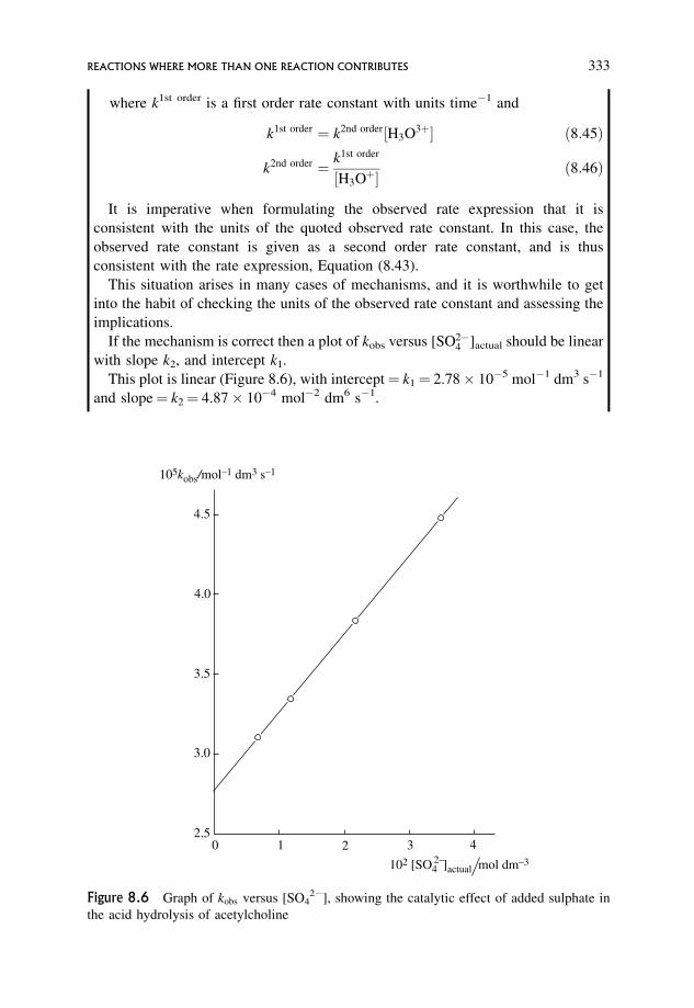
where k1st order is a first order rate constant with units time�1 and
k1st order ¼ k2nd order½H3O3þ� ð8:45Þ
k2nd order ¼ k1st order
½H3Oþ� ð8:46Þ
It is imperative when formulating the observed rate expression that it is
consistent with the units of the quoted observed rate constant. In this case, the
observed rate constant is given as a second order rate constant, and is thus
consistent with the rate expression, Equation (8.43).
This situation arises in many cases of mechanisms, and it is worthwhile to get
into the habit of checking the units of the observed rate constant and assessing the
implications.
If the mechanism is correct then a plot of kobs versus [SO2�4 ]actual should be linear
with slope k2, and intercept k1.
This plot is linear (Figure 8.6), with intercept¼ k1¼ 2.78 10�5 mol�1 dm3 s�1
and slope¼ k2¼ 4.87 10�4 mol�2 dm6 s�1.
102 [SO4 ]actual mol dm_3
105kobs/mol_1 dm3 s_1
4.5
4.0
3.5
3.0
2.50 1 2 3 4
2_
Figure 8.6 Graph of kobs versus [SO42�], showing the catalytic effect of added sulphate in
the acid hydrolysis of acetylcholine
REACTIONS WHERE MORE THAN ONE REACTION CONTRIBUTES 333
Note. The units of k2 are those for a third order rate constant, consistent with the
contribution from the SO2�4 catalysis being
k2½HEþ�½H3Oþ�actual½SO2�4 �actual
The following questions relate to important points.
� Why should the rate expressions be written in terms of [H3Oþ]actual and
[SO2�4 ]actual rather than in terms of the total concentrations?
� Comment on the relative values of the two contributions to the rate.
The answers are the following.
� The SO2�4 is added to an acid solution, and is involved in the equilibrium
H3OþðaqÞ þ SO2�4 ðaqÞ�! �HSO�4 ðaqÞ þ H2OðaqÞ
Significant amounts of SO2�4 will be removed by protonation giving HSO�4 , and
this will also reduce the amount of H3Oþ, and so the actual concentrations will
be significantly less than the total concentrations of these species. The actual
concentrations can be calculated from the equilibrium quotient
½HSO�4 �actual
½H3Oþ�actual½SO2�4 �actual
� �equil
ð8:47Þ
with corrections for non-ideality.
� k2[SO2�4 ] ranges from 3.4 10�6 to 1.7 10�5 mol�1 dm3 s�1, which are values
comparable to k1 and not negligible compared with it. This is what would be
expected for a catalytic reaction.
This is an anion-catalysed mechanism analogous to metal ion or cation-catalysed
reactions. But the kinetically equivalent mechanism of general acid hydrolysis by
HSO�4 , analogous to general base hydrolysis, is also possible (Section 8.1.3 and
Problem 8.3).
Since reaction is carried out in acid solution with added SO2�4 there will be a
substantial amount of HSO�4 present in equilibrium with H3Oþ and SO2�4 .
SO2�4 ðaqÞ þ H3OþðaqÞ�! �HSO2�
4 ðaqÞ þ H2OðlÞ
K ¼ ½HSO�4 �actual
½H3Oþ�actual½SO2�4 �actual
� �equil
ð8:48Þ
with corrections for non-ideality.
334 EXAMPLES OF REACTIONS IN SOLUTION
A mechanism involving HSO�4 can be written
HEþ þ H3Oþ �!k1productsþ H3Oþ
HEþ þ HSO�4 �!k2
productsþ HSO�4
The mechanistic rate,
� d½HEþ�dt
¼ k1½HEþ�½H3Oþ�actual þ k2½HEþ�½HSO�4 �actual ð8:49Þ
The observed rate is again written as a second order process:
� d½HEþ�dt
¼ kobs½HEþ�½H3Oþ�actual ð8:41Þ
; kobs ¼ k1 þ k2
½HSO�4 �actual
½H3Oþ�actual
ð8:50Þ
Substituting for [HSO�4 ]actual in terms of K and [SO2�4 ] gives
kobs ¼ k1 þ k2K½SO2�4 �actual ð8:51Þ
which is algebraically equivalent to the expression deduced by assuming catalysis is
by SO2�4 , and these mechanisms cannot be distinguished kinetically.
� kobs ¼ k1 þ k2½SO2�4 �actual ð8:42Þ
¼ k1 þ constant½SO2�4 �actual ð8:52Þ
� kobs ¼ k1 þ k2K½SO2�4 �actual ð8:51Þ
¼ k1 þ constant½SO2�4 �actual ð8:53Þ
The catalytic mechanisms proposed are
HEþ þ H3Oþ þ SO2�4 �!
k2productsþ H3Oþ þ SO2�
4
HEþ þ HSO�4 �!k2
productsþ HSO�4
The second is more likely since it suggests that only two species have to come
together to form the activated complex, whereas, in the first, three would have to
come together: a less likely process. However, there are charges involved. The first
REACTIONS WHERE MORE THAN ONE REACTION CONTRIBUTES 335
mechanism is electrostatically more favourable, since it involves the reaction of
singly charged cations with a doubly charged anion.
Whichever the mechanism, the activated complex will have the same constitution
and charge.
8.2 More Complex Kinetic Situations Involving
Reactants in Equilibrium with Each Other
and Undergoing Reaction
There are a large number of inorganic and organic reactions which have these problems
in the analysis. Three reactions will illustrate the ways to tackle the analysis.
8.2.1 A further look at the base hydrolysis of glycine ethyl ester
as an illustration of possible problems
The simple treatment of Section 8.1.2 gave the mechanistic rate quoted as
� d½E�total
dt¼ k1½E�actual½OH��actual þ k2½HEþ�actual½OH��actual ð8:17Þ
The observed rate quoted was
� d½E�total
dt¼ kobs½E�total½OH��actual ð8:18Þ
giving
kobs½E�total ¼ k1½E�actual þ k2½HEþ�actual ð8:20Þ
kobs ¼ k1
½E�actual
½E�total
þ k2
½HEþ�actual
½E�total
ð8:21Þ
Since Kb is small, it was possible to approximate [E]actual¼ [E]total to give the simple
relationship
kobs ¼ k1 þ k2
Kb
½OH��actual
ð8:26Þ
The approximation made for the glycine ethyl ester may not be justified in
situations where there is a significant amount of all species involved in the
equilibrium present, and a more rigorous analysis must be used.
In the present case, the way forward is to recognize that ½E�actual=½E�total is the
fraction of the original ester that is unprotonated, ½HEþ�actual=½E�total is the fraction of
336 EXAMPLES OF REACTIONS IN SOLUTION
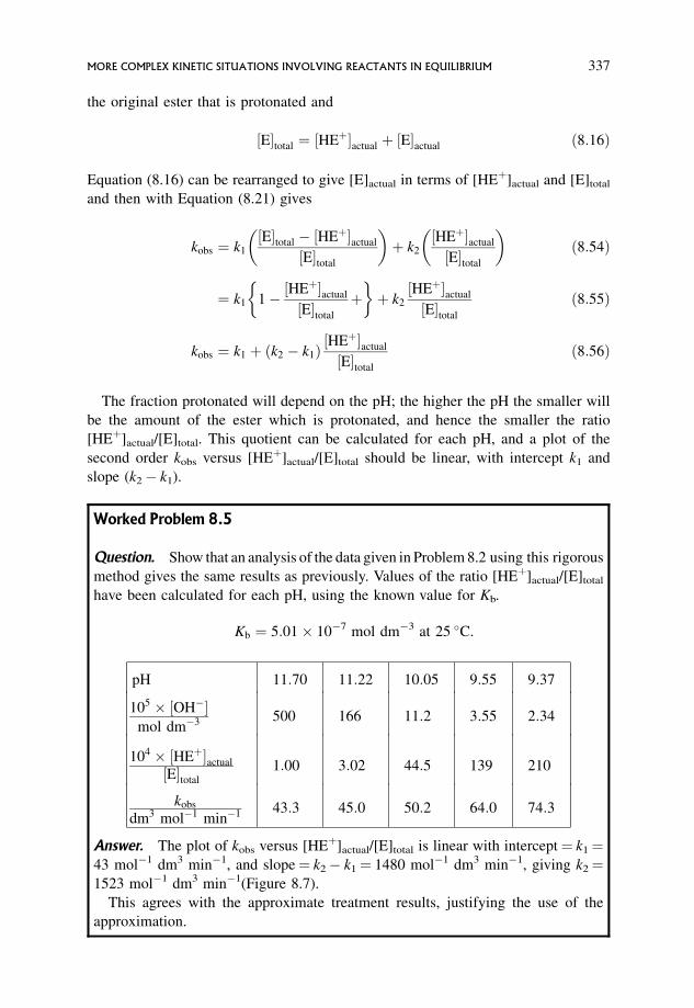
the original ester that is protonated and
½E�total ¼ ½HEþ�actual þ ½E�actual ð8:16Þ
Equation (8.16) can be rearranged to give [E]actual in terms of [HEþ]actual and [E]total
and then with Equation (8.21) gives
kobs ¼ k1
½E�total � ½HEþ�actual
½E�total
� �þ k2
½HEþ�actual
½E�total
� �ð8:54Þ
¼ k1 1� ½HEþ�actual
½E�total
þ� �
þ k2
½HEþ�actual
½E�total
ð8:55Þ
kobs ¼ k1 þ ðk2 � k1Þ½HEþ�actual
½E�total
ð8:56Þ
The fraction protonated will depend on the pH; the higher the pH the smaller will
be the amount of the ester which is protonated, and hence the smaller the ratio
[HEþ]actual/[E]total. This quotient can be calculated for each pH, and a plot of the
second order kobs versus [HEþ]actual/[E]total should be linear, with intercept k1 and
slope (k2� k1).
Worked Problem 8.5
Question. Show that an analysis of the data given in Problem 8.2 using this rigorous
method gives the same results as previously. Values of the ratio [HEþ]actual/[E]total
have been calculated for each pH, using the known value for Kb.
Kb ¼ 5:01 10�7 mol dm�3 at 25 �C.
pH 11:70 11:22 10:05 9:55 9:37
105 ½OH��mol dm�3 500 166 11:2 3:55 2:34
104 ½HEþ�actual
½E�total
1:00 3:02 44:5 139 210
kobs
dm3 mol�1 min�1 43:3 45:0 50:2 64:0 74:3
Answer. The plot of kobs versus [HEþ]actual/[E]total is linear with intercept¼ k1¼43 mol�1 dm3 min�1, and slope¼ k2� k1¼ 1480 mol�1 dm3 min�1, giving k2¼1523 mol�1 dm3 min�1(Figure 8.7).
This agrees with the approximate treatment results, justifying the use of the
approximation.
MORE COMPLEX KINETIC SITUATIONS INVOLVING REACTANTS IN EQUILIBRIUM 337

Another important point about analysis of experimental data and the drawing of graphs
Another way of getting a relationship between kobs and quantities calculated from Kb
and the pH will not result in a useful graph. This alternative procedure uses
Equation (8.16) in terms of [E]actual and [E]total rather than [HEþ]actual and [E]total.
½E�actual=½E�total is the fraction of the original ester which is unprotonated,
½HEþ�actual=½E�total is the fraction of the original ester which is protonated and
½HEþ�actual ¼ ½E�total � ½E�actual ð8:57Þ
Substitution of this relation into Equation (8.21),
kobs ¼ k1
½E�actual
½E�total
þ k2
½HEþ�actual
½E�total
ð8:21Þ
gives
kobs ¼ k1
½E�actual
½E�total
þ k2
½E�total
½E�total
� ½E�actual
½E�total
� �ð8:58Þ
¼ k2 þ ðk1 � k2Þ½E�actual
½E�total
ð8:59Þ
Figure 8.7 Graph of kobs versus ½HEþ�actual=½E�total for the base hydrolysis of glycine ethyl
ester
338 EXAMPLES OF REACTIONS IN SOLUTION
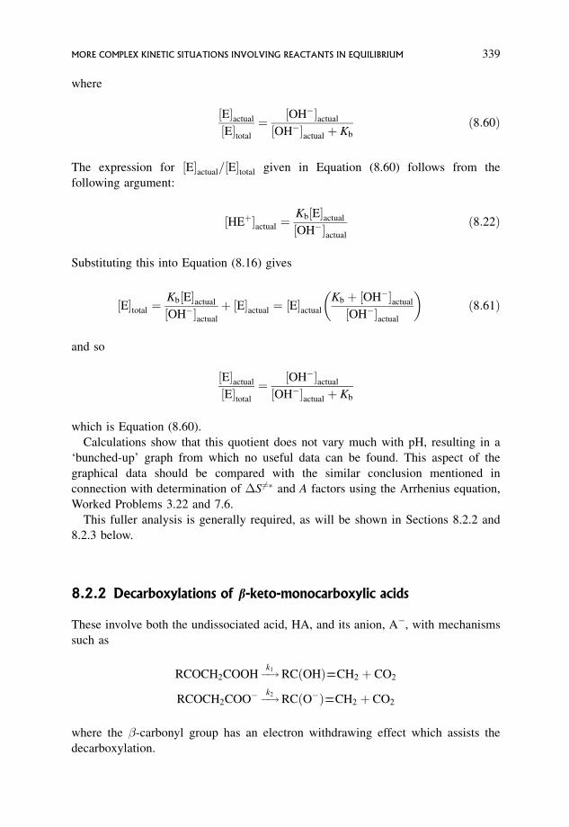
where
½E�actual
½E�total
¼ ½OH��actual
½OH��actual þ Kb
ð8:60Þ
The expression for ½E�actual=½E�total given in Equation (8.60) follows from the
following argument:
½HEþ�actual ¼Kb½E�actual
½OH��actual
ð8:22Þ
Substituting this into Equation (8.16) gives
½E�total ¼Kb½E�actual
½OH��actual
þ ½E�actual ¼ ½E�actual
Kb þ ½OH��actual
½OH��actual
� �ð8:61Þ
and so
½E�actual
½E�total
¼ ½OH��actual
½OH��actual þ Kb
which is Equation (8.60).
Calculations show that this quotient does not vary much with pH, resulting in a
‘bunched-up’ graph from which no useful data can be found. This aspect of the
graphical data should be compared with the similar conclusion mentioned in
connection with determination of �S6¼� and A factors using the Arrhenius equation,
Worked Problems 3.22 and 7.6.
This fuller analysis is generally required, as will be shown in Sections 8.2.2 and
8.2.3 below.
8.2.2 Decarboxylations of b-keto-monocarboxylic acids
These involve both the undissociated acid, HA, and its anion, A�, with mechanisms
such as
RCOCH2COOH�!k1RCðOHÞ����CH2 þ CO2
RCOCH2COO� �!k2RCðO�Þ����CH2 þ CO2
where the �-carbonyl group has an electron withdrawing effect which assists the
decarboxylation.
MORE COMPLEX KINETIC SITUATIONS INVOLVING REACTANTS IN EQUILIBRIUM 339

C
OH
O
CCH2
OR C
OH
CH2
RCO2+
C
O O
CCH2
OR C
O
CH2
RCO2+
The mechanistic rate is
þ d½CO2�dt
¼ � d½HA�total
dt¼ k1½HA�actual þ k2½A��actual ð8:62Þ
where
½HA�total ¼ ½HA�actual þ ½A��actual ð8:63Þ
and
Ka ¼½H3Oþ�actual½A��actual
½HA�actual
� �equil
ð8:64Þ
The observed rate expression is given in terms of the total [HA]:
þ d½CO2�dt
¼ � d½HA�total
dt¼ kobs½HA�total ð8:65Þ
kobs ¼ k1
½HA�actual
½HA�total
þ k2
½A��actual
½HA�total
ð8:66Þ
This is algebraically identical to that for the glycine ester hydrolysis, Equation
(8.21). However, in this case the acid ionization constant is sufficiently large for
significant amounts of both ionized and un-ionized acid to be present, and no
approximations can be made, so that since
½HA�actual ¼ ½HA�total � ½A��actual ð8:67Þ
kobs ¼ k1
½HA�total � ½A��actual
½HA�total
� �þ k2
½A��actual
½HA�total
ð8:68Þ
¼ k1
½HA�total
½HA�total
� k1
½A��actual
½HA�total
þ k2
½A��actual
½HA�total
ð8:69Þ
¼ k1 þ ðk2 � k1Þ½A��actual
½HA�total
ð8:70Þ
340 EXAMPLES OF REACTIONS IN SOLUTION
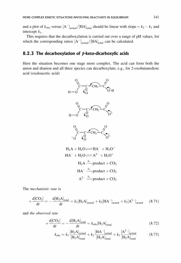
and a plot of kobs versus ½A��actual=½HA�total should be linear with slope¼ k2� k1 and
intercept k1.
This requires that the decarboxylation is carried out over a range of pH values, for
which the corresponding ratios ½A��actual=½HA�total can be calculated.
8.2.3 The decarboxylation of b-keto-dicarboxylic acids
Here the situation becomes one stage more complex. The acid can form both the
anion and dianion and all three species can decarboxylate, e.g., for 2-oxobutanedioic
acid (oxaloacetic acid)
C C
O
CH2 C
O
O H
O
OH
C C
O
CH2 C
O
O
O
OH
C C
O
CH2 C
O
O
O
O
H2Aþ H2O�! �HA� þ H3Oþ
HA� þ H2O�! �A2� þ H3Oþ
H2A�!k1productþ CO2
HA� �!k2productþ CO2
A2� �!k3productþ CO2
The mechanistic rate is
þ d½CO2�dt
¼ � d½H2A�total
dt¼ k1½H2A�actual þ k2½HA��actual þ k3½A2��actual ð8:71Þ
and the observed rate
þ d½CO2�dt
¼ � d½H2A�total
dt¼ kobs½H2A�total ð8:72Þ
kobs ¼ k1
½H2A�actual
½H2A�total
þ k2
½HA��actual
½H2A�total
þ k3
½A2��actual
½H2A�total
ð8:73Þ
MORE COMPLEX KINETIC SITUATIONS INVOLVING REACTANTS IN EQUILIBRIUM 341
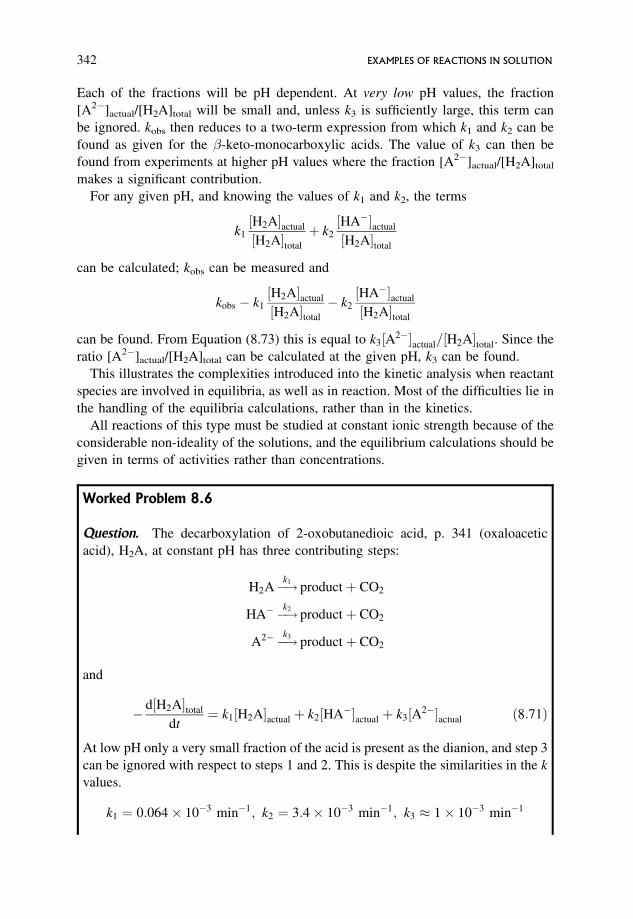
Each of the fractions will be pH dependent. At very low pH values, the fraction
[A2�]actual/[H2A]total will be small and, unless k3 is sufficiently large, this term can
be ignored. kobs then reduces to a two-term expression from which k1 and k2 can be
found as given for the �-keto-monocarboxylic acids. The value of k3 can then be
found from experiments at higher pH values where the fraction [A2�]actual/[H2A]total
makes a significant contribution.
For any given pH, and knowing the values of k1 and k2, the terms
k1
½H2A�actual
½H2A�total
þ k2
½HA��actual
½H2A�total
can be calculated; kobs can be measured and
kobs � k1
½H2A�actual
½H2A�total
� k2
½HA��actual
½H2A�total
can be found. From Equation (8.73) this is equal to k3½A2��actual=½H2A�total. Since the
ratio [A2�]actual/[H2A]total can be calculated at the given pH, k3 can be found.
This illustrates the complexities introduced into the kinetic analysis when reactant
species are involved in equilibria, as well as in reaction. Most of the difficulties lie in
the handling of the equilibria calculations, rather than in the kinetics.
All reactions of this type must be studied at constant ionic strength because of the
considerable non-ideality of the solutions, and the equilibrium calculations should be
given in terms of activities rather than concentrations.
Worked Problem 8.6
Question. The decarboxylation of 2-oxobutanedioic acid, p. 341 (oxaloacetic
acid), H2A, at constant pH has three contributing steps:
H2A�!k1productþ CO2
HA� �!k2productþ CO2
A2� �!k3productþ CO2
and
� d½H2A�total
dt¼ k1½H2A�actual þ k2½HA��actual þ k3½A2��actual ð8:71Þ
At low pH only a very small fraction of the acid is present as the dianion, and step 3
can be ignored with respect to steps 1 and 2. This is despite the similarities in the k
values.
k1 ¼ 0:064 10�3 min�1; k2 ¼ 3:4 10�3 min�1; k3 1 10�3 min�1
342 EXAMPLES OF REACTIONS IN SOLUTION
� Calculate the contribution to the reaction for each of the steps 1, 2 and 3 when
the concentrations of the three species are
½H2A�actual ¼ 2:80 10�2 mol dm�3; ½HA��actual ¼ 1:36 10�3 mol dm�3;
½A2��actual ¼ 1:76 10�6 mol dm�3:
� If this experiment was carried out with the total acid concentration equal to
0.0294 mol dm�3, find the overall observed rate constant.
� Why is it necessary to carry out the reaction at constant pH?
Answer.
(a) � d½H2A�total
dt¼ k1½H2A�actual þ k2½HA��actual þ k3½A2��actual ð8:71Þ
¼ 0:064 10�3 min�1 2:80 10�2 mol dm�3
þ 3:4 10�3 min�1 1:36 10�3 mol dm�3
þ 1 10�3 min�1 1:76 10�6 mol dm�3
¼ f1:79 10�6 þ 4:62 10�6
þ 1:76 10�9g mol dm�3 min�1
¼ 6:41 10�6 mol dm�3 min�1
Hence, at this pH, the contribution to the overall rate from the monoanion is
greater than that for the undissociated acid and the contribution from the
dianion can be neglected.
Note. It is the product of rate constant and actual concentration which is
important.
(b) � d½H2A�total
dt¼ kobs½H2A�total ¼ 6:41 10�6 mol dm�3 min�1
½H2A�total ¼ 0:0294 mol dm�3
kobs ¼6:41 10�6 mol dm�3 min�1
0:0294 mol dm�3¼ 2:18 10�4 min�1
(c) It is vital to keep the pH constant because the concentrations of the reacting
species are involved in acid–base equilibria, which are governed by the pH.
This is something which must not be overlooked when reactants are involved in
other equilibria or interlinked equilibria.
MORE COMPLEX KINETIC SITUATIONS INVOLVING REACTANTS IN EQUILIBRIUM 343
8.3 Metal Ion Catalysis
Many reactions of biological interest are catalysed by metal ions. Simple model
systems for these complex reactions have been studied, e.g. metal-ion-catalysed
decarboxylations of dicarboxylic acids, and metal-ion-catalysed hydrolyses.
In the decarboxylations, the catalytic activity is associated with the formation of a
metal ion complex, formed with the carbonyl group and a carboxylic acid group
which does not decarboxylate.
C C
O
CH2 C
O
O
O
O
M2+
The formation of the complex creates a very strong electron-withdrawing group
which helps the withdrawal of the electrons from the carbon–carbon bond which is
breaking. Catalysis results because this electron-withdrawing effect is much stronger
than the effect of the anion in the uncatalysed decarboxylations.
A similar situation arises when the metal-ion-catalysed base hydrolyses of
aminoacids and peptides are studied. Such hydrolyses contrast with the base
hydrolyses of simple esters, which are not catalysed by metal ions. Again, metal
ion complexes with the aminoacid esters or the peptides are involved in the
catalyses. The presence of the metal ion increases the electron-withdrawing power
of the carbonyl group and helps attack by the hydroxide ion, leading to efficient
hydrolysis.
Both the metal ion decarboxylations and the metal ion hydrolyses can be handled
in similar fashion.
CH2
NH2
M2+
O
C OEt
OH
CH2
NH2 O
C OEt
OH
Worked Problem 8.7
Question. The metal ion hydrolysis of glycine ethyl ester NH2CH2COOC2H5 (the
simplest amino-acid ester) can involve three equilibria and four concurrent
reactions.
Let E represent NH2CH2COOC2H5, and HEþ represent NHþ3 CH2COOC2H5.
Eþ H3Oþ �! �HEþ þ H2O
K ¼ ½HEþ�actual
½E�actual½H3Oþ�actual
ð8:74Þ
344 EXAMPLES OF REACTIONS IN SOLUTION
EþMzþ �! �EMzþ
K1 ¼½EMzþ�actual
½E�actual½Mzþ�actual
ð8:75Þ
2EþMzþ �! �E2Mzþ
K2 ¼½E2Mzþ�actual
½E�2actual½Mzþ�actual
!equil
ð8:76Þ
Eþ OH� ! products
HEþ þ OH� ! products
Eþ OH� þMzþ ! productsþMzþ
2Eþ OH� þMzþ ! productsþMzþ
This scheme can be simplified by carrying out the reaction at sufficiently high pH
values for the reaction of OH� with the protonated ester to be ignored, and by
having Mzþ in such high excess that only the 1:1 chelate is formed. Under these
circumstances, the reaction simplifies to
Eþ OH� �!k1products
Eþ OH� þMzþ �!kcatproductsþMzþ
Formulate the mechanistic rate expression and from this find an expression for the
dependence of kobs on [Mzþ] which will allow k1 and kcat to be found.
Answer. Mechanistic rate:
� d½E�actual
dt¼ k1½E�actual½OH��actual þ kcat½E�actual½OH��actual½Mzþ�actual ð8:77Þ
This can be simplified as follows.
� Reaction is carried out at pH values such that [HEþ]actual is very low, and so
[E]actual can be approximated to [E]total.
� Since the metal ion is present in large excess, [Mzþ]actual can be approximated to
[Mzþ]total.
� The reaction is carried out in a pH-stat, where the pH is kept constant by
progressive addition of OH� as reaction occurs. [OH�]actual is thus kept constant
throughout. The observed rate is thus in terms of [OH�]actual.
METAL ION CATALYSIS 345
� These facts result in the mechanistic rate now being
� d½E�total
dt¼ k1½E�total½OH��actual þ kcat½E�total½OH��actual½Mzþ�total ð8:78Þ
The observed rate is
� d½E�total
dt¼ kobs½E�total½OH��actual ð8:79Þ
kobs ¼ k1 þ kcat½Mzþ�total ð8:80Þ
If the mechanism is correct, then a plot of kobs versus [Mzþ]total will be linear with
slope¼ kcat and intercept¼ k1.
The value of k1 from this plot should be equal to the value of k1 for reaction in the
absence of metal ions.
8.4 Other Common Mechanisms
Many inorganic mechanisms involve pre-equilibria (Section 3.22).
� A �! �k1
k�1
B�!k2C
� Aþ B �! �k1
k�1
C�!k2D
� Aþ B �! �k1
C
Cþ X�!k2D
A mathematical analysis of such mechanisms shows that simple kinetics is only found
when the equilibrium is set up rapidly and maintained throughout the reaction. In all
other circumstances, complex kinetics would be expected, and computer analysis of
the experimental data would be required. Fortunately, for most inorganic mechanisms
the equilibrium is set up rapidly and maintained, and simple kinetics is observed.
The situations discussed in this book are for reactions where the pre-equilibrium is
set up rapidly and maintained.
8.4.1 The simplest mechanism
A �! �k1
k�1
B�!k2C
can be used to illustrate some of the features of such reaction types.
� If the pre-equilibrium is established rapidly, then the step
B�!k2C
346 EXAMPLES OF REACTIONS IN SOLUTION
will be rate determining, and reaction reduces effectively to B! C, so that
mechanistic rate ¼ þ d½C�dt¼ k2½B�actual ð8:81Þ
� The kinetic requirements for this to be the case are
k1 or k�1 must be large
and k1þ k�1� k2
� When the setting up of the equilibrium is fast, and then maintained throughout the
reaction, then throughout the reaction
� ½B�actual at time t
½A�actual at time t
¼ K ð8:82Þ
[B]actual at time t is the equilibrium value of [B]actual at that time, and likewise for A.
� B is always being removed to form C, and so throughout reaction both A and B are
being removed. [A]actual and [B]actual are, therefore, not constant throughout the
reaction, but vary continually throughout reaction, even though their quotient
½B�actual at time t=½A�actual at time t always remains constant.
The analysis follows a similar pattern for all types of pre-equilibrium reaction, and
this will be illustrated below with each step in the argument being listed.
8.4.2 Kinetic analysis of the simplest mechanism
The mechanism
A �! �k1
k�1
B�!k2C
has the following features.
� Reaction is found to be first order in A.
� The total stoichiometric amount of A present at any given time may be regarded as
made up of the actual amounts of A and B present at that time, so that
½A�total ¼ ½A�actual þ ½B�actual ð8:83Þ
These actual concentrations which are present in the solution are related by the
equilibrium constant:
K ¼ ½B�actual
½A�actual
� �equil
ð8:84Þ
OTHER COMMON MECHANISMS 347
so that
½A�actual ¼ ½B�actual=K ð8:85Þ
and
½B�actual ¼ K½A�actual ð8:86Þ
� From the mechanism
increase in ½B�actual ¼ decrease in ½A�actual � increase in ½C�
þ d½B�actual
dt¼ � d½A�actual
dt� d½C�
dtð8:87Þ
þ d½C�dt¼ � d½A�actual
dt� d½B�actual
dt¼ � dð½A�actual þ ½B�actualÞ
dt¼ � d½A�total
dtð8:88Þ
The rate-determining step is B�!k2C
mechanistic rate ¼ þ d½C�dt¼ k2½B�actual ð8:81Þ
; � dð½A�actual þ ½B�actualÞdt
¼ � d½A�total
dt¼ k2½B�actual ð8:89Þ
� It is necessary to find an expression for [B]actual in terms of constants, e.g. K, or k1
and k2, and/or known quantities, e.g. [A]total.
So substitute for [A]actual in Equation (8.83) to get an expression for [B]actual in
terms of K and [A]total:
½A�total ¼½B�actual
Kþ ½B�actual ¼ ½B�actual
1þ K
K
� �ð8:90Þ
½B�actual ¼K
1þ K
� �½A�total ð8:91Þ
� The mechanistic rate can now be given as
rate of reaction ¼ þ d½C�dt¼ � d½A�total
dt¼ k2½B�actual ¼ k2
K
1þ K
� �½A�total ð8:92Þ
� It now remains to decide how the experimental rate is to be followed. It is
important to pay attention to this step in the analysis.
There are four possibilities:
1. in terms of the product, [C]
2. in terms of the total [A]
348 EXAMPLES OF REACTIONS IN SOLUTION
3. in terms of the actual A present, [A]actual
4. in terms of the actual B present, [B]actual.
The chemistry of the system will determine which is chosen, but usually the change
in [A]total or [C] is monitored when
� observed rate ¼ � d½A�total
dt¼ þ d½C�
dt¼ kobs½A�total ð8:93Þ
But note: in the examples in Problems 8.3 and 8.7, the rate is given in terms of an
actual concentration of a reactant. In these examples the experimental technique
actually measured the actual concentration rather than the total concentration. Care
must be taken to distinguish between these two situations.
� If the mechanism is correct, then the observed and mechanistic rates must be equal and
kobs½A�total ¼ k2
K
1þ K
� �½A�total ð8:94Þ
kobs ¼ k2
K
1þ K
� �ð8:95Þ
Since the reaction is first order in A, a plot of loge[A]total at time t versus t is linear
with slope ¼ �kobs ¼ �k2K=ð1þ KÞ , from which k2 can be found, provided K is
known independently. K¼ k1/k�1, and other experiments will be required to deter-
mine k1 and k�1 individually.
There are two limiting cases for kobs.
� If K is large, then most of the reactant present is in the form of B, and 1þ K K,
so that kobs k2.
� If K is small, then there is very little B present and 1þ K 1, so that kobs¼ k2K.
Worked Problem 8.8
Question. Formulate expressions for kobs for the above mechanism for cases
where the overall rate is found by following
� [B]actual with time
� [A]actual with time.
Answer.
� Following [B]actual with time:
observed rate of reaction ¼ � d½B�actual
dt¼ kobs½B�actual ð8:96Þ
OTHER COMMON MECHANISMS 349
mechanistic rate of reaction ¼ þ d½C�dt¼ � d½A�actual
dt� d½B�actual
dt
¼ � dð½A�actual þ ½B�actualÞdt
ð8:97Þ
From Equation ð8:85Þ : ½A�actual ¼ ½B�actual=K
þ d½C�dt¼ � dð½A�actual þ ½B�actualÞ
dt
¼ �d½B�actual
Kþ ½B�actual
n odt
¼ � d½B�actual
dt
1þ K
K
� �ð8:98Þ
� d½B�actual
dt¼ K
1þ K
d½C�dt
ð8:99Þ
þ d½C�dt¼ k2½B�actual ð8:81Þ
� d½B�actual
dt¼ k2K
1þ K½B�actual ð8:100Þ
If the mechanism is correct, Equations (8.96) and (8.100) are equal, giving:
kobs ¼k2K
1þ Kð8:101Þ
� Following [A]actual with time,
observed rate ¼ � d½A�actual
dt¼ kobs½A�actual ð8:102Þ
mechanistic rate ¼ þ d½C�dt¼ � dð½A�actual þ ½B�actualÞ
dt
¼ � dð½A�actual þ K½A�actualÞdt
ð8:103Þ
¼ � d½A�actual
dt1þ Kf g ð8:104Þ
� d½A�actual
dt¼ 1
1þ K
d½C�dt
ð8:105Þ
d½C�dt¼ k2½B�actual ð8:81Þ
� d½A�actual
dt¼ k2
1þ K½B�actual ð8:106Þ
If the mechanism is correct, then the observed and mechanistic rates are equal:
kobs½A�actual ¼k2
1þ K½B�actual ð8:107Þ
kobs ¼k2
1þ K
½B�actual
½A�actual
¼ k2K
1þ Kð8:108Þ
350 EXAMPLES OF REACTIONS IN SOLUTION
The analyses in Section 8.4.2 and in this problem are all self-consistent, as is shown
by all resulting in the same expression for kobs.
Note how absolutely crucial it is to specify exactly how the experimental rate is
found, and how vital it is to distinguish between actual and total concentrations.
8.4.3 A slightly more complex scheme
Aþ B �! �k1
k�1
C�!k2D
This is a typical inorganic mechanism where there is a pre-equilibrium formation of
an ion pair or complex, followed by reaction to product, e.g.
Cr3þðaqÞ þ edta4�ðaqÞ �! �k1
k�1
CrðedtaÞ�ðaqÞ
CrðedtaÞ�ðaqÞ�!k2products
The forward step of the reversible reaction is second order, and this poses the usual
problems.
If the initial conditions correspond to
� [A]0¼ [B]0, then the situation is similar to that discussed in Section 8.4.2, except
that the forward step 1 is second order;
� [A]0 6¼ [B]0, then complex kinetics are observed, and computer solutions are
necessary.
However, if either A or B is held in excess then
� the forward step of formation of C is pseudo-first order.
Normally one of the reactants is held in excess, and the reaction is studied under
pseudo-first order conditions, when
� the forward step of formation of C is pseudo-first order;
� the reaction is found to be first order in the reactant not in excess, and this is the
reactant which is monitored throughout;
� the reaction is found to be of complex kinetics for the substance in excess, with the
observed pseudo-first order rate constant depending on the concentration of this
substance in a complex manner;
� this is resolved by carrying out experiments at various concentrations, all of which
are in excess.
OTHER COMMON MECHANISMS 351

8.4.4 Standard procedure for determining the expression for kobsfor the given mechanism (Section 8.4.3)
This should be compared with the previous analysis (Section 8.4.2).
� In this reaction a decision has to be made as to which of the reactants will always
be held in excess. The analysis is similar whichever is chosen. Let reactant in
excess be B.
� The total amounts of A and B are distributed by the equilibrium into the actual
amounts of A, B and C present at any given time.
These are related by the equilibrium constant, K:
K ¼ ½C�actual
½A�actual½B�actual
� �equil
ð8:109Þ
so that
½A�actual ¼½C�actual
K½B�actual
ð8:110Þ
and
½C�actual ¼ K½A�actual½B�actual ð8:111Þ
� From the mechanism
increase in ½C�actual ¼ decrease in ½A�actual � increase in ½D�
þ d½C�actual
dt¼ � d½A�actual
dt� d½D�
dtð8:112Þ
þ d½D�dt¼� d½A�actual
dt� d½C�actual
dt¼� dð½A�actualþ½C�actualÞ
dt¼� d½A�total
dtð8:113Þ
Since the rate-determining step is C�!k2D
mechanistic rate ¼ þ d½D�dt¼ k2½C�actual ð8:114Þ
; � d½A�total
dt¼ k2½C�actual ð8:115Þ
352 EXAMPLES OF REACTIONS IN SOLUTION
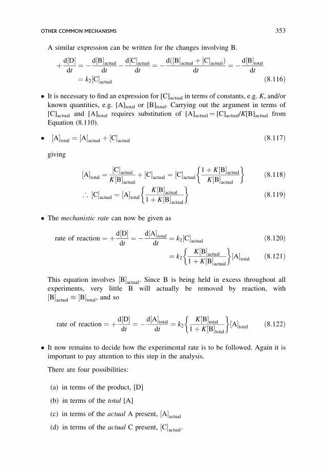
A similar expression can be written for the changes involving B.
þ d½D�dt¼ � d½B�actual
dt� d½C�actual
dt¼ � dð½B�actual þ ½C�actualÞ
dt¼ � d½B�total
dt
¼ k2½C�actual ð8:116Þ
� It is necessary to find an expression for [C]actual in terms of constants, e.g. K, and/or
known quantities, e.g. [A]total or [B]total. Carrying out the argument in terms of
[C]actual and [A]total requires substitution of [A]actual¼ [C]actual/K[B]actual from
Equation (8.110).
� ½A�total ¼ ½A�actual þ ½C�actual ð8:117Þ
giving
½A�total ¼½C�actual
K½B�actual
þ ½C�actual ¼ ½C�actual
1þ K½B�actual
K½B�actual
� �ð8:118Þ
; ½C�actual ¼ ½A�total
K½B�actual
1þ K½B�actual
� �ð8:119Þ
� The mechanistic rate can now be given as
rate of reaction ¼ þ d½D�dt¼ � d½A�total
dt¼ k2½C�actual ð8:120Þ
¼ k2
K½B�actual
1þ K½B�actual
� �½A�total ð8:121Þ
This equation involves ½B�actual. Since B is being held in excess throughout all
experiments, very little B will actually be removed by reaction, with
½B�actual ½B�total, and so
rate of reaction ¼ þ d½D�dt¼ � d½A�total
dt¼ k2
K½B�total
1þ K½B�total
� �½A�total ð8:122Þ
� It now remains to decide how the experimental rate is to be followed. Again it is
important to pay attention to this step in the analysis.
There are four possibilities:
(a) in terms of the product, [D]
(b) in terms of the total [A]
(c) in terms of the actual A present, ½A�actual
(d) in terms of the actual C present, ½C�actual.
OTHER COMMON MECHANISMS 353
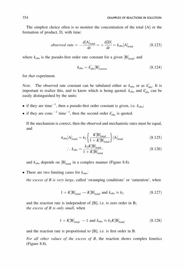
The simplest choice often is to monitor the concentration of the total [A] or the
formation of product, D, with time:
observed rate ¼ � d½A�total
dt¼ þ d½D�
dt¼ kobs½A�total ð8:123Þ
where kobs is the pseudo-first order rate constant for a given ½B�total, and
kobs ¼ k0obs½B�excess ð8:124Þ
for that experiment.
Note. The observed rate constant can be tabulated either as kobs or as k0obs. It is
important to realize this, and to know which is being quoted. kobs and k0obs can be
easily distinguished by the units:
� if they are time�1, then a pseudo-first order constant is given, i.e. kobs;
� if they are conc.�1 time�1, then the second order k0obs is quoted.
If the mechanism is correct, then the observed and mechanistic rates must be equal,
and
kobs½A�total ¼ k2
K½B�total
1þ K½B�total
� �½A�total ð8:125Þ
; kobs ¼k2K½B�total
1þ K½B�total
ð8:126Þ
and kobs depends on ½B�total in a complex manner (Figure 8.8).
� There are two limiting cases for kobs:
the excess of B is very large, called ‘swamping conditions’ or ‘saturation’, when
1þ K½B�total ! K½B�total and kobs k2 ð8:127Þ
and the reaction rate is independent of [B], i.e. is zero order in B;
the excess of B is only small, when
1þ K½B�total ! 1 and kobs k2K½B�total ð8:128Þ
and the reaction rate is proportional to [B], i.e. is first order in B.
For all other values of the excess of B, the reaction shows complex kinetics
(Figure 8.8).
354 EXAMPLES OF REACTIONS IN SOLUTION
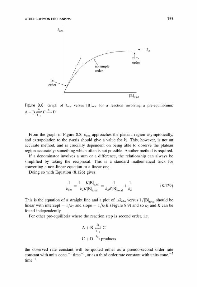
From the graph in Figure 8.8, kobs approaches the plateau region asymptotically,
and extrapolation to the y-axis should give a value for k2. This, however, is not an
accurate method, and is crucially dependent on being able to observe the plateau
region accurately: something which often is not possible. Another method is required.
If a denominator involves a sum or a difference, the relationship can always be
simplified by taking the reciprocal. This is a standard mathematical trick for
converting a non-linear equation to a linear one.
Doing so with Equation (8.126) gives
1
kobs
¼ 1þ K½B�total
k2K½B�total
¼ 1
k2K½B�total
þ 1
k2
ð8:129Þ
This is the equation of a straight line and a plot of 1/kobs versus 1=½B�total should be
linear with intercept ¼ 1=k2 and slope ¼ 1=k2K (Figure 8.9) and so k2 and K can be
found independently.
For other pre-equilibria where the reaction step is second order, i.e.
Aþ B �! �k1
k�1
C
Cþ D�!k2products
the observed rate constant will be quoted either as a pseudo-second order rate
constant with units conc.�1 time�1, or as a third order rate constant with units conc.�2
time�1.
no simpleorder
1storder
kobs
k2
zeroorder
[B]total
Figure 8.8 Graph of kobs versus [B]total for a reaction involving a pre-equilibrium:
Aþ B �! �k1
k�1
C�!k2D
OTHER COMMON MECHANISMS 355
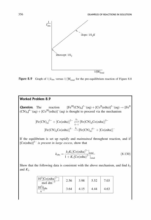
Worked Problem 8.9
Question. The reaction [FeIII(CN)6]3�(aq)þ [CoII(edta)]2�(aq)! [FeII
(CN)6]4�(aq)þ [CoIII(edta)]�(aq) is thought to proceed via the mechanism
½FeðCNÞ6�3� þ ½CoðedtaÞ�2� �! �
k1
k�1½FeðCNÞ6CoðedtaÞ�5�
½FeðCNÞ6CoðedtaÞ�5� �!k2 ½FeðCNÞ6�4� þ ½CoðedtaÞ��
If the equilibrium is set up rapidly and maintained throughout reaction, and if
[Co(edta)]2� is present in large excess, show that
kobs ¼k2K1½CoðedtaÞ2��total
1þ K1½CoðedtaÞ2��total
ð8:130Þ
Show that the following data is consistent with the above mechanism, and find k2
and K1.
103½CoðedtaÞ2��mol dm�3 2:56 3:98 5:52 7:03
103kobs
s�1 3:64 4:15 4:44 4:63
intercept: 1/k2
1/[B]total
slope: 1/k2K
kobs
1
Figure 8.9 Graph of 1=kobs versus 1=½B�total for the pre-equilibrium reaction of Figure 8.8
356 EXAMPLES OF REACTIONS IN SOLUTION
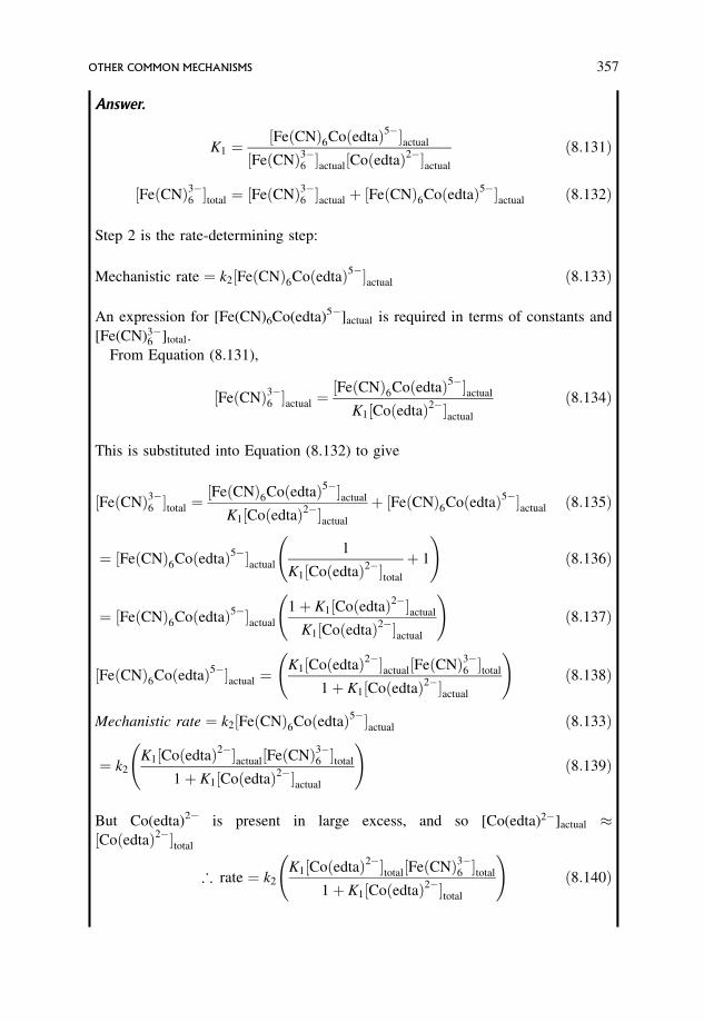
Answer.
K1 ¼½FeðCNÞ6CoðedtaÞ5��actual
½FeðCNÞ3�6 �actual½CoðedtaÞ2��actual
ð8:131Þ
½FeðCNÞ3�6 �total ¼ ½FeðCNÞ3�6 �actual þ ½FeðCNÞ6CoðedtaÞ5��actual ð8:132Þ
Step 2 is the rate-determining step:
Mechanistic rate ¼ k2½FeðCNÞ6CoðedtaÞ5��actual ð8:133Þ
An expression for [Fe(CN)6Co(edta)5�]actual is required in terms of constants and
[Fe(CN)3�6 ]total.
From Equation (8.131),
½FeðCNÞ3�6 �actual ¼½FeðCNÞ6CoðedtaÞ5��actual
K1½CoðedtaÞ2��actual
ð8:134Þ
This is substituted into Equation (8.132) to give
½FeðCNÞ3�6 �total ¼½FeðCNÞ6CoðedtaÞ5��actual
K1½CoðedtaÞ2��actual
þ ½FeðCNÞ6CoðedtaÞ5��actual ð8:135Þ
¼ ½FeðCNÞ6CoðedtaÞ5��actual
1
K1½CoðedtaÞ2��total
þ 1
!ð8:136Þ
¼ ½FeðCNÞ6CoðedtaÞ5��actual
1þ K1½CoðedtaÞ2��actual
K1½CoðedtaÞ2��actual
!ð8:137Þ
½FeðCNÞ6CoðedtaÞ5��actual ¼K1½CoðedtaÞ2��actual½FeðCNÞ3�6 �total
1þ K1½CoðedtaÞ2��actual
!ð8:138Þ
Mechanistic rate ¼ k2½FeðCNÞ6CoðedtaÞ5��actual ð8:133Þ
¼ k2
K1½CoðedtaÞ2��actual½FeðCNÞ3�6 �total
1þ K1½CoðedtaÞ2��actual
!ð8:139Þ
But Co(edta)2� is present in large excess, and so [Co(edta)2�]actual ½CoðedtaÞ2��total
; rate ¼ k2
K1½CoðedtaÞ2��total½FeðCNÞ3�6 �total
1þ K1½CoðedtaÞ2��total
!ð8:140Þ
OTHER COMMON MECHANISMS 357
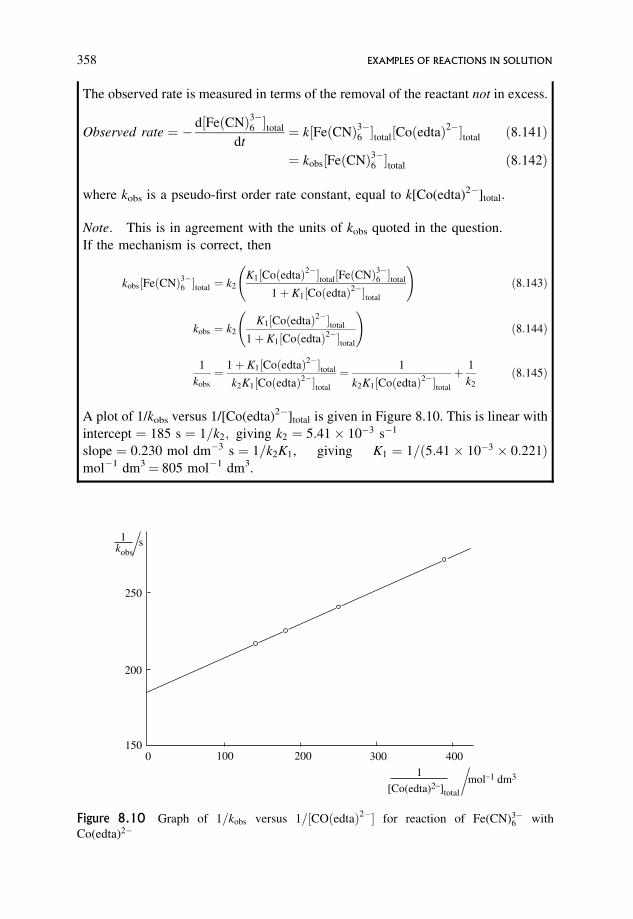
The observed rate is measured in terms of the removal of the reactant not in excess.
Observed rate ¼ � d½FeðCNÞ3�6 �total
dt¼ k½FeðCNÞ3�6 �total½CoðedtaÞ2��total ð8:141Þ
¼ kobs½FeðCNÞ3�6 �total ð8:142Þ
where kobs is a pseudo-first order rate constant, equal to k[Co(edta)2�]total.
Note. This is in agreement with the units of kobs quoted in the question.
If the mechanism is correct, then
kobs½FeðCNÞ3�6 �total ¼ k2
K1½CoðedtaÞ2��total½FeðCNÞ3�6 �total
1þ K1½CoðedtaÞ2��total
!ð8:143Þ
kobs ¼ k2
K1½CoðedtaÞ2��total
1þ K1½CoðedtaÞ2��total
!ð8:144Þ
1
kobs
¼ 1þ K1½CoðedtaÞ2��total
k2K1½CoðedtaÞ2��total
¼ 1
k2K1½CoðedtaÞ2��total
þ 1
k2
ð8:145Þ
A plot of 1/kobs versus 1/[Co(edta)2�]total is given in Figure 8.10. This is linear with
intercept ¼ 185 s ¼ 1=k2; giving k2 ¼ 5:41 10�3 s�1
slope ¼ 0:230 mol dm�3 s ¼ 1=k2K1, giving K1 ¼ 1=ð5:41 10�3 0:221Þmol�1 dm3¼ 805 mol�1 dm3.
250
200
1500 100 200 300 400
kobs
1 s
[Co(edta)2_]total
1 mol
_1 dm3
Figure 8.10 Graph of 1=kobs versus 1=½COðedtaÞ2�� for reaction of Fe(CN)3�6 with
Co(edta)2�
358 EXAMPLES OF REACTIONS IN SOLUTION
8.5 Steady States in Solution Reactions
Some reactions in solution can be analysed by the steady state treatment, and the
principles discussed for the gas phase are also relevant to solution reactions.
� A proposed mechanism is written down;
� highly reactive intermediates are present;
� these intermediates are present in very, very low but almost constant concentra-
tions;
� þd½I�ss=dt ¼ 0;
� steady state equations are set up for each intermediate;
� these are solved to give each [I]ss;
� the mechanistic rate is then derived, and compared with the observed rate.
8.5.1 Types of reaction for which a steady state
treatment could be relevant
Although free radical reactions are found less often in solution than in the gas phase,
they do occur, and are generally handled by steady state methods. There are also
organic and inorganic reactions that involve non-radical intermediates in steady state
concentrations. These intermediates are often produced by an initial reversible
reaction, or a set of reversible reactions. This can be compared with the pre-equilibria
discussed in Section 8.4, where the intermediates are in equilibrium concentrations.
The steady state treatment is also used extensively in acid–base catalysis and in
enzyme kinetics.
Question. How could a distinction be made between the situation where a pre-
equilibrium is set up and maintained throughout reaction, and one where a steady
state is set up?
Answer. If there are measurable concentrations of intermediates, then there will not
be a steady state. If the intermediates are detectable but are in very, very low
concentrations, then a steady state is probably set up. This could also be a pre-
equilibrium state with the equilibrium lying very far to the left, in which case the
equilibrium concentration of intermediate probably approximates to a steady state.
An analysis of the algebraic forms of the rate expressions for the steady state and pre-
equilibrium situations may be needed to see whether they can be distinguished
(Section 8.5.2 and Problem 8.11).
STEADY STATES IN SOLUTION REACTIONS 359
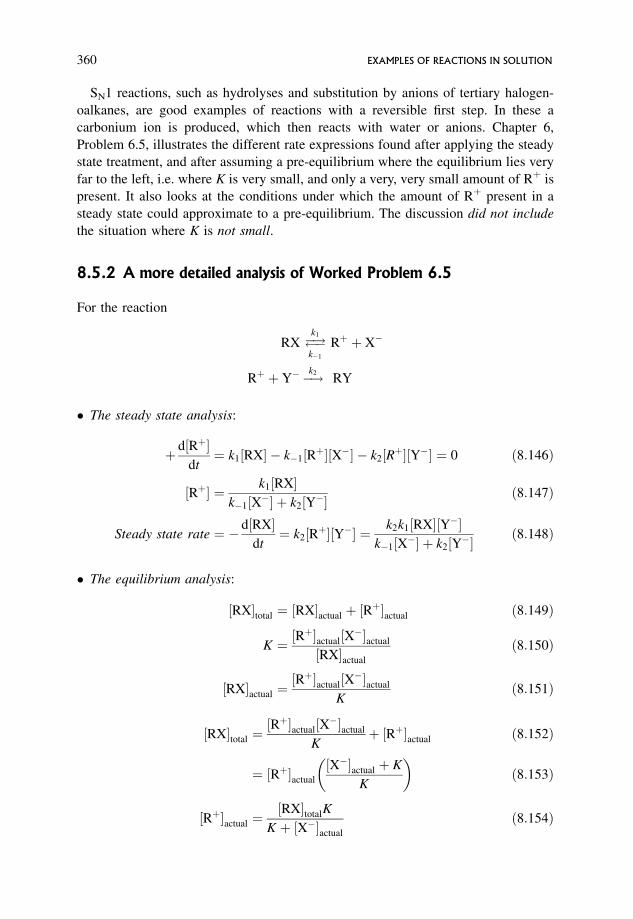
SN1 reactions, such as hydrolyses and substitution by anions of tertiary halogen-
oalkanes, are good examples of reactions with a reversible first step. In these a
carbonium ion is produced, which then reacts with water or anions. Chapter 6,
Problem 6.5, illustrates the different rate expressions found after applying the steady
state treatment, and after assuming a pre-equilibrium where the equilibrium lies very
far to the left, i.e. where K is very small, and only a very, very small amount of Rþ is
present. It also looks at the conditions under which the amount of Rþ present in a
steady state could approximate to a pre-equilibrium. The discussion did not include
the situation where K is not small.
8.5.2 A more detailed analysis of Worked Problem 6.5
For the reaction
RX �! �k1
k�1
Rþ þ X�
Rþ þ Y� �!k2RY
� The steady state analysis:
þ d½Rþ�dt¼ k1½RX� � k�1½Rþ�½X�� � k2½Rþ�½Y�� ¼ 0 ð8:146Þ
½Rþ� ¼ k1½RX�k�1½X�� þ k2½Y��
ð8:147Þ
Steady state rate ¼ � d½RX�dt¼ k2½Rþ�½Y�� ¼
k2k1½RX�½Y��k�1½X�� þ k2½Y��
ð8:148Þ
� The equilibrium analysis:
½RX�total ¼ ½RX�actual þ ½Rþ�actual ð8:149Þ
K ¼ ½Rþ�actual½X��actual
½RX�actual
ð8:150Þ
½RX�actual ¼½Rþ�actual½X��actual
Kð8:151Þ
½RX�total ¼½Rþ�actual½X��actual
Kþ ½Rþ�actual ð8:152Þ
¼ ½Rþ�actual
½X��actual þ K
K
� �ð8:153Þ
½Rþ�actual ¼½RX�totalK
K þ ½X��actual
ð8:154Þ
360 EXAMPLES OF REACTIONS IN SOLUTION
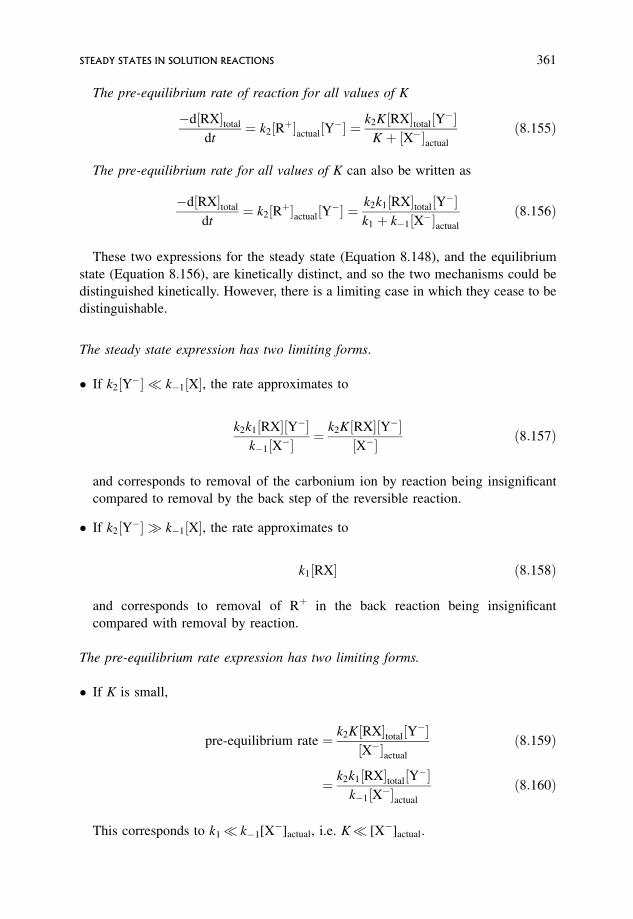
The pre-equilibrium rate of reaction for all values of K
�d½RX�total
dt¼ k2½Rþ�actual½Y�� ¼
k2K½RX�total½Y��K þ ½X��actual
ð8:155Þ
The pre-equilibrium rate for all values of K can also be written as
�d½RX�total
dt¼ k2½Rþ�actual½Y�� ¼
k2k1½RX�total½Y��k1 þ k�1½X��actual
ð8:156Þ
These two expressions for the steady state (Equation 8.148), and the equilibrium
state (Equation 8.156), are kinetically distinct, and so the two mechanisms could be
distinguished kinetically. However, there is a limiting case in which they cease to be
distinguishable.
The steady state expression has two limiting forms.
� If k2½Y�� � k�1½X�, the rate approximates to
k2k1½RX�½Y��k�1½X��
¼ k2K½RX�½Y��½X�� ð8:157Þ
and corresponds to removal of the carbonium ion by reaction being insignificant
compared to removal by the back step of the reversible reaction.
� If k2½Y�� � k�1½X�, the rate approximates to
k1½RX� ð8:158Þ
and corresponds to removal of Rþ in the back reaction being insignificant
compared with removal by reaction.
The pre-equilibrium rate expression has two limiting forms.
� If K is small,
pre-equilibrium rate ¼ k2K½RX�total½Y��½X��actual
ð8:159Þ
¼ k2k1½RX�total½Y��k�1½X��actual
ð8:160Þ
This corresponds to k1� k�1[X�]actual, i.e. K� [X�]actual.
STEADY STATES IN SOLUTION REACTIONS 361
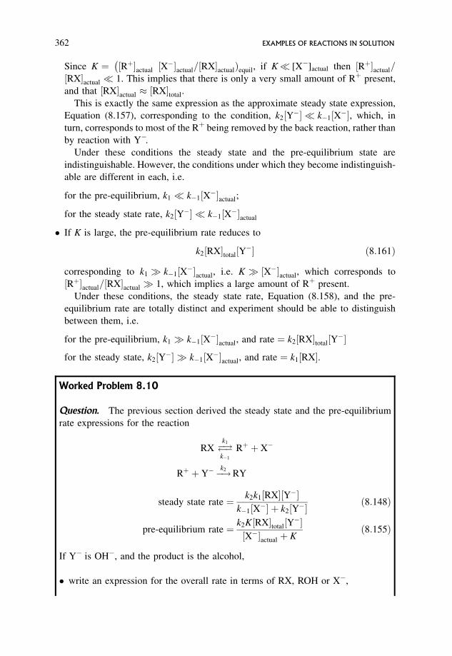
Since K ¼ ½Rþ�actual
�½X��actual=½RX�actualÞequil, if K� [X�]actual then ½Rþ�actual=
½RX�actual � 1. This implies that there is only a very small amount of Rþ present,
and that ½RX�actual ½RX�total.
This is exactly the same expression as the approximate steady state expression,
Equation (8.157), corresponding to the condition, k2½Y�� � k�1½X��, which, in
turn, corresponds to most of the Rþ being removed by the back reaction, rather than
by reaction with Y�.
Under these conditions the steady state and the pre-equilibrium state are
indistinguishable. However, the conditions under which they become indistinguish-
able are different in each, i.e.
for the pre-equilibrium, k1 � k�1½X��actual;
for the steady state rate, k2½Y�� � k�1½X��actual
� If K is large, the pre-equilibrium rate reduces to
k2½RX�total½Y�� ð8:161Þ
corresponding to k1 � k�1½X��actual, i.e. K � ½X��actual, which corresponds to
½Rþ�actual=½RX�actual � 1, which implies a large amount of Rþ present.
Under these conditions, the steady state rate, Equation (8.158), and the pre-
equilibrium rate are totally distinct and experiment should be able to distinguish
between them, i.e.
for the pre-equilibrium, k1 � k�1½X��actual, and rate ¼ k2½RX�total½Y��
for the steady state, k2½Y�� � k�1½X��actual, and rate ¼ k1½RX�.
Worked Problem 8.10
Question. The previous section derived the steady state and the pre-equilibrium
rate expressions for the reaction
RX �! �k1
k�1
Rþ þ X�
Rþ þ Y� �!k2RY
steady state rate ¼ k2k1½RX�½Y��k�1½X�� þ k2½Y��
ð8:148Þ
pre-equilibrium rate ¼ k2K½RX�total½Y��½X��actual þ K
ð8:155Þ
If Y� is OH�, and the product is the alcohol,
� write an expression for the overall rate in terms of RX, ROH or X�,
362 EXAMPLES OF REACTIONS IN SOLUTION
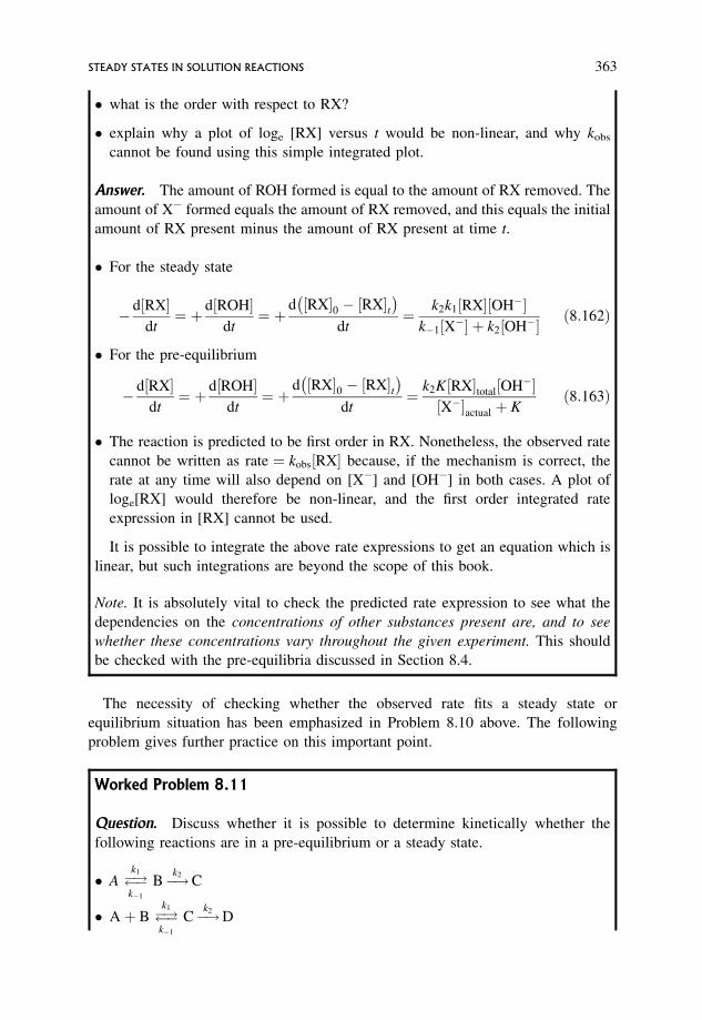
� what is the order with respect to RX?
� explain why a plot of loge [RX] versus t would be non-linear, and why kobs
cannot be found using this simple integrated plot.
Answer. The amount of ROH formed is equal to the amount of RX removed. The
amount of X� formed equals the amount of RX removed, and this equals the initial
amount of RX present minus the amount of RX present at time t.
� For the steady state
� d½RX�dt¼ þ d½ROH�
dt¼ þ
d ½RX�0 � ½RX�t� �
dt¼ k2k1½RX�½OH��
k�1½X�� þ k2½OH�� ð8:162Þ
� For the pre-equilibrium
� d½RX�dt¼ þ d½ROH�
dt¼ þ
d ½RX�0 � ½RX�t� �
dt¼ k2K½RX�total½OH��½X��actual þ K
ð8:163Þ
� The reaction is predicted to be first order in RX. Nonetheless, the observed rate
cannot be written as rate ¼ kobs½RX� because, if the mechanism is correct, the
rate at any time will also depend on [X�] and [OH�] in both cases. A plot of
loge[RX] would therefore be non-linear, and the first order integrated rate
expression in [RX] cannot be used.
It is possible to integrate the above rate expressions to get an equation which is
linear, but such integrations are beyond the scope of this book.
Note. It is absolutely vital to check the predicted rate expression to see what the
dependencies on the concentrations of other substances present are, and to see
whether these concentrations vary throughout the given experiment. This should
be checked with the pre-equilibria discussed in Section 8.4.
The necessity of checking whether the observed rate fits a steady state or
equilibrium situation has been emphasized in Problem 8.10 above. The following
problem gives further practice on this important point.
Worked Problem 8.11
Question. Discuss whether it is possible to determine kinetically whether the
following reactions are in a pre-equilibrium or a steady state.
� A �! �k1
k�1
B�!k2C
� Aþ B �! �k1
k�1
C�!k2D
STEADY STATES IN SOLUTION REACTIONS 363
Answer.
� For A �! �k1
k�1
B�!k2C
the pre-equilibrium rate was shown to be
� d½A�dt¼ k2
K
1þ K
� �½A�total ð8:92Þ
¼ k2k1½A�k�1 þ k1
ð8:164Þ
Applying the steady state treatment to B:
þ d½B�dt¼ k1½A� � k�1½B� � k2½B� ¼ 0 ð8:165Þ
½B� ¼ k1½A�k�1 þ k2
ð8:166Þ
� d½A�dt¼ k2½B� ¼
k2k1½A�k�1 þ k2
ð8:167Þ
The steady state and pre-equilibrium rate expressions are kinetically equivalent,
so it is impossible to distinguish between them experimentally, but note that the
expressions are different, because the denominators are different.
� In contrast, for the reaction
Aþ B �! �k1
k�1
C�!k2D
it is possible to distinguish between the steady state and pre-equilibrium
situations.
The pre-equilibrium rate of reaction in the presence of excess B is
� d½A�total
dt¼ k2
K½B�total
1þ K½B�total
� �½A�total ð8:122Þ
¼ k2k1½B�total½A�total
k�1 þ k1½B�total
ð8:168Þ
The observed rate
� d½A�total
dt¼ kobs½A�total½B�total ð8:169Þ
; kobs ¼k2k1
k�1 þ k1½B�total
ð8:170Þ
364 EXAMPLES OF REACTIONS IN SOLUTION
The steady state expression for the rate of reaction
þ d½C�dt¼ k1½A�½B� � k�1½C� � k2½C� ¼ 0 ð8:171Þ
½C� ¼ k1½A�½B�k�1 þ k2
ð8:172Þ
� d½A�dt¼ k2½C� ¼
k2k1½A�½B�k�1 þ k2
¼ kobs½A�½B� ð8:173Þ
kobs ¼k2k1
k�1 þ k2
ð8:174Þ
These two situations can easily be distinguished kinetically. The steady state rate
has a denominator which is independent of [B], while the pre-equilibrium rate
depends on [B].
It is essential to check whether a reaction is in a steady state or in a pre-equilibrium
state. If this is to be done kinetically, it is vital to derive the mechanistic rate
expressions and see whether they are kinetically equivalent or not. If they are, then
recourse to non-kinetic methods becomes necessary.
In all of these reactions the species involved in the reversible reactions are
progressively used up with time. However, there are reactions such as acid–base
catalysis and enzyme catalysis where one of the species in the reversible reaction is
the catalyst, and as such is regenerated so that the total catalyst concentration remains
constant throughout the whole of the reaction. In such cases it is often essential to use
initial rates or rates at various stages during reaction for analysis.
8.6 Enzyme Kinetics
Enzymes are proteins which act as catalysts in many reactions of biological and
biochemical importance. Because of their efficiency, enzymes are effective at very
low concentrations, of the order of 10�8 mol dm�3 to 10�10 mol dm�3. The molecule
whose reaction is being studied is called the substrate, and typical concentrations are
10�6 mol dm�3 or greater. This means that the substrate is always in large excess.
The simplest mechanistic scheme describing the action of an enzyme is
Eþ S �! �k1
k�1
ES �! �k2
k�2
Eþ product
Enzyme kinetics are usually studied as initial rates and step ð�2Þ can then be ignored.
ENZYME KINETICS 365
The rate of reaction is defined as
k2½ES�actual ð8:175Þ
and
½E�total ¼ ½E�actual þ ½ES�actual ð8:176Þ
As in so many of the examples studied previously, the aim is to express ½ES�actual in
terms of ½E�total and constants. In this case a steady state is assumed, and the constants
will be the rate constants k1, k�1 and k2. Assuming a steady state,
þ d½ES�dt¼ k1½E�actual½S� � k�1½ES�actual � k2½ES�actual ¼ 0 ð8:177Þ
k�1½ES�actual þ k2½ES�actual ¼ k1½E�actual½S� ð8:178Þ
½ES�actual ¼k1½E�actual½S�
k�1 þ k2
ð8:179Þ
An expression for ½ES�actual in terms of constants and ½E�total is required, and this
requires elimination of ½E�actual from Equations (8.177)–(8.179)
Equation (8.177) can be rewritten using Equation (8.176) in the form
½E�actual ¼ ½E�total � ½ES�actual ð8:180Þk�1½ES�actual þ k2½ES�actual ¼ k1½S�f½E�total � ½ES�actualg ð8:181Þ
¼ k1½E�total½S� � k1½ES�actual½S� ð8:182Þ½ES�actual k1½S� þ k�1 þ k2f g ¼ k1½E�total½S� ð8:183Þ
½ES�actual ¼k1½E�total½S�
k1½S� þ k�1 þ k2
ð8:184Þ
giving
rate ¼ k2k1½E�total½S�k1½S� þ k�1 þ k2
¼ k2½E�total½S�½S� þ ðk�1 þ k2Þ=k1
ð8:185Þ
This is equivalent to
rate ¼ const½S�½S� þ const:0
ð8:186Þ
This expression shows complex kinetics with no simple order in S, and none of
the standard integrated expressions is applicable; compare this with the similar
situation given in Problem 8.10. Analysis using rate/concentration data is necessary,
and, to eliminate effects of any contribution from the reverse of step 2, initial rates are
used.
366 EXAMPLES OF REACTIONS IN SOLUTION
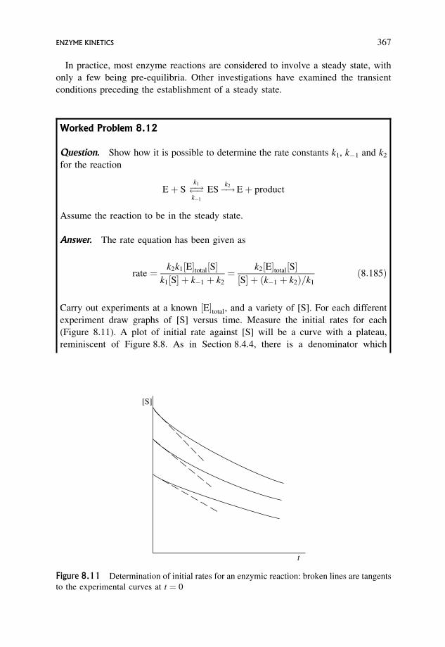
In practice, most enzyme reactions are considered to involve a steady state, with
only a few being pre-equilibria. Other investigations have examined the transient
conditions preceding the establishment of a steady state.
Worked Problem 8.12
Question. Show how it is possible to determine the rate constants k1, k�1 and k2
for the reaction
Eþ S �! �k1
k�1
ES�!k2Eþ product
Assume the reaction to be in the steady state.
Answer. The rate equation has been given as
rate ¼ k2k1½E�total½S�k1½S� þ k�1 þ k2
¼ k2½E�total½S�½S� þ ðk�1 þ k2Þ=k1
ð8:185Þ
Carry out experiments at a known ½E�total, and a variety of [S]. For each different
experiment draw graphs of [S] versus time. Measure the initial rates for each
(Figure 8.11). A plot of initial rate against [S] will be a curve with a plateau,
reminiscent of Figure 8.8. As in Section 8.4.4, there is a denominator which
[S]
t
Figure 8.11 Determination of initial rates for an enzymic reaction: broken lines are tangents
to the experimental curves at t ¼ 0
ENZYME KINETICS 367
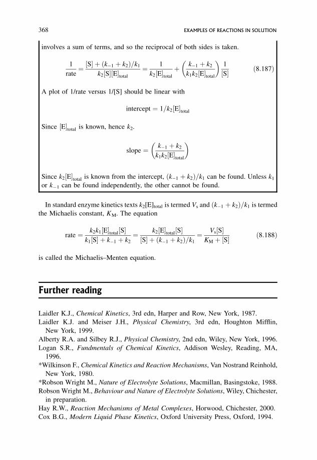
involves a sum of terms, and so the reciprocal of both sides is taken.
1
rate¼ ½S� þ ðk�1 þ k2Þ=k1
k2½S�½E�total
¼ 1
k2½E�total
þ k�1 þ k2
k1k2½E�total
� �1
½S� ð8:187Þ
A plot of 1/rate versus 1/[S] should be linear with
intercept ¼ 1=k2½E�total
Since ½E�total is known, hence k2.
slope ¼ k�1 þ k2
k1k2½E�total
� �
Since k2½E�total is known from the intercept, ðk�1 þ k2Þ=k1 can be found. Unless k1
or k�1 can be found independently, the other cannot be found.
In standard enzyme kinetics texts k2[E]total is termed Vs and ðk�1 þ k2Þ=k1 is termed
the Michaelis constant, KM. The equation
rate ¼ k2k1½E�total½S�k1½S� þ k�1 þ k2
¼ k2½E�total½S�½S� þ ðk�1 þ k2Þ=k1
¼ Vs½S�KM þ ½S�
ð8:188Þ
is called the Michaelis–Menten equation.
Further reading
Laidler K.J., Chemical Kinetics, 3rd edn, Harper and Row, New York, 1987.
Laidler K.J. and Meiser J.H., Physical Chemistry, 3rd edn, Houghton Mifflin,
New York, 1999.
Alberty R.A. and Silbey R.J., Physical Chemistry, 2nd edn, Wiley, New York, 1996.
Logan S.R., Fundmentals of Chemical Kinetics, Addison Wesley, Reading, MA,
1996.
*Wilkinson F., Chemical Kinetics and Reaction Mechanisms, Van Nostrand Reinhold,
New York, 1980.
*Robson Wright M., Nature of Electrolyte Solutions, Macmillan, Basingstoke, 1988.
Robson Wright M., Behaviour and Nature of Electrolyte Solutions, Wiley, Chichester,
in preparation.
Hay R.W., Reaction Mechanisms of Metal Complexes, Horwood, Chichester, 2000.
Cox B.G., Modern Liquid Phase Kinetics, Oxford University Press, Oxford, 1994.
368 EXAMPLES OF REACTIONS IN SOLUTION
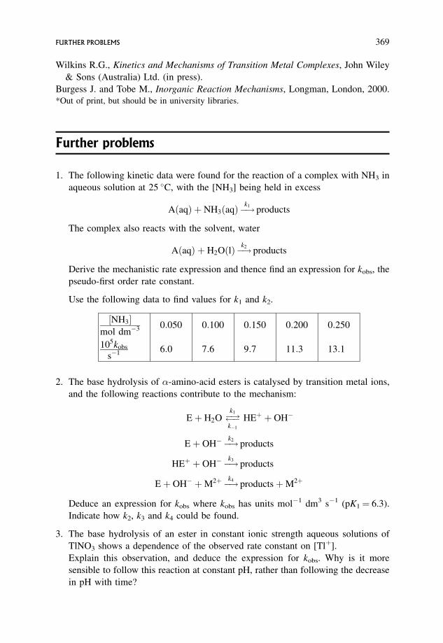
Wilkins R.G., Kinetics and Mechanisms of Transition Metal Complexes, John Wiley
& Sons (Australia) Ltd. (in press).
Burgess J. and Tobe M., Inorganic Reaction Mechanisms, Longman, London, 2000.*Out of print, but should be in university libraries.
Further problems
1. The following kinetic data were found for the reaction of a complex with NH3 in
aqueous solution at 25 �C, with the [NH3] being held in excess
AðaqÞ þ NH3ðaqÞ�!k1products
The complex also reacts with the solvent, water
AðaqÞ þ H2OðlÞ�!k2products
Derive the mechanistic rate expression and thence find an expression for kobs, the
pseudo-first order rate constant.
Use the following data to find values for k1 and k2.
½NH3�mol dm�3 0:050 0:100 0:150 0:200 0:250
105kobs
s�1 6:0 7:6 9:7 11:3 13:1
2. The base hydrolysis of �-amino-acid esters is catalysed by transition metal ions,
and the following reactions contribute to the mechanism:
Eþ H2O �! �k1
k�1
HEþ þ OH�
Eþ OH� �!k2products
HEþ þ OH� �!k3products
Eþ OH� þM2þ �!k4productsþM2þ
Deduce an expression for kobs where kobs has units mol�1 dm3 s�1 (pK1¼ 6.3).
Indicate how k2, k3 and k4 could be found.
3. The base hydrolysis of an ester in constant ionic strength aqueous solutions of
TlNO3 shows a dependence of the observed rate constant on [Tlþ].
Explain this observation, and deduce the expression for kobs. Why is it more
sensible to follow this reaction at constant pH, rather than following the decrease
in pH with time?
FURTHER PROBLEMS 369
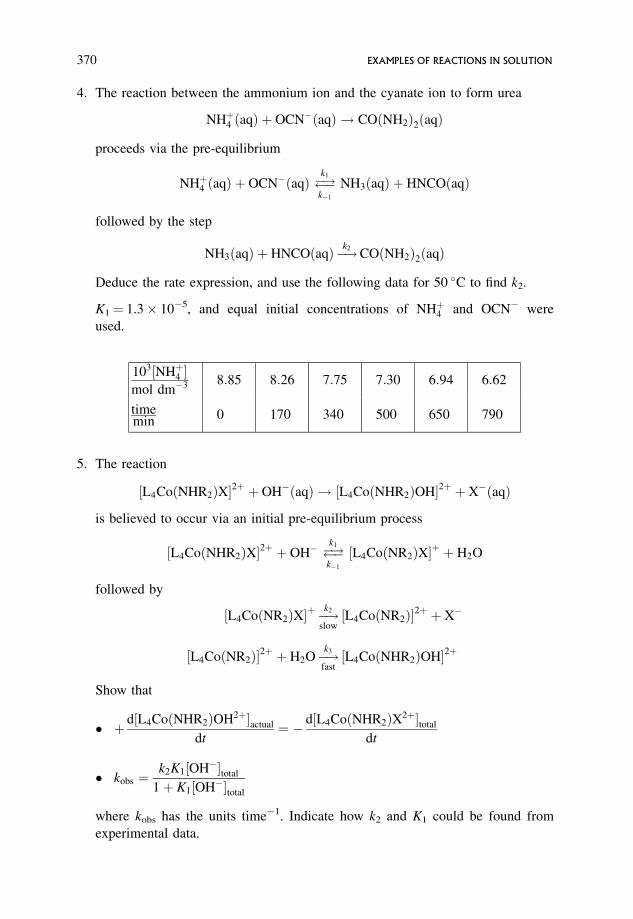
4. The reaction between the ammonium ion and the cyanate ion to form urea
NHþ4 ðaqÞ þ OCN�ðaqÞ ! COðNH2Þ2ðaqÞ
proceeds via the pre-equilibrium
NHþ4 ðaqÞ þ OCN�ðaqÞ �! �k1
k�1
NH3ðaqÞ þ HNCOðaqÞ
followed by the step
NH3ðaqÞ þ HNCOðaqÞ�!k2COðNH2Þ2ðaqÞ
Deduce the rate expression, and use the following data for 50 �C to find k2.
K1¼ 1.3 10�5, and equal initial concentrations of NHþ4 and OCN� were
used.
103½NHþ4 �mol dm�3 8:85 8:26 7:75 7:30 6:94 6:62
timemin
0 170 340 500 650 790
5. The reaction
½L4CoðNHR2ÞX�2þ þ OH�ðaqÞ ! ½L4CoðNHR2ÞOH�2þ þ X�ðaqÞ
is believed to occur via an initial pre-equilibrium process
½L4CoðNHR2ÞX�2þ þ OH� �! �k1
k�1
½L4CoðNR2ÞX�þ þ H2O
followed by
½L4CoðNR2ÞX�þ �!k2
slow½L4CoðNR2Þ�2þ þ X�
½L4CoðNR2Þ�2þ þ H2O�!k3
fast½L4CoðNHR2ÞOH�2þ
Show that
� þ d½L4CoðNHR2ÞOH2þ�actual
dt¼ � d½L4CoðNHR2ÞX2þ�total
dt
� kobs ¼k2K1½OH��total
1þ K1½OH��total
where kobs has the units time�1. Indicate how k2 and K1 could be found from
experimental data.
370 EXAMPLES OF REACTIONS IN SOLUTION
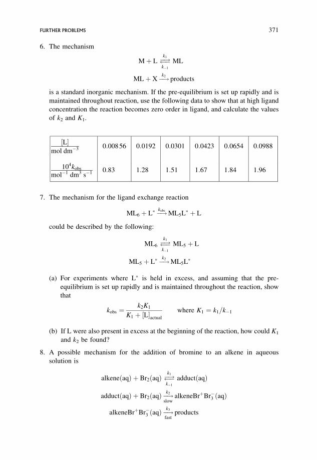
6. The mechanism
Mþ L �! �k1
k�1
ML
MLþ X�!k2products
is a standard inorganic mechanism. If the pre-equilibrium is set up rapidly and is
maintained throughout reaction, use the following data to show that at high ligand
concentration the reaction becomes zero order in ligand, and calculate the values
of k2 and K1.
½L�mol dm�3 0:00856 0:0192 0:0301 0:0423 0:0654 0:0988
104kobs
mol�1 dm3 s�1 0:83 1:28 1:51 1:67 1:84 1:96
7. The mechanism for the ligand exchange reaction
ML6 þ L� �!kobsML5L� þ L
could be described by the following:
ML6�! �
k1
k�1
ML5 þ L
ML5 þ L� �!k2ML5L�
(a) For experiments where L� is held in excess, and assuming that the pre-
equilibrium is set up rapidly and is maintained throughout the reaction, show
that
kobs ¼k2K1
K1 þ ½L�actual
where K1 ¼ k1=k�1
(b) If L were also present in excess at the beginning of the reaction, how could K1
and k2 be found?
8. A possible mechanism for the addition of bromine to an alkene in aqueous
solution is
alkeneðaqÞ þ Br2ðaqÞ �! �k1
k�1
adductðaqÞ
adductðaqÞ þ Br2ðaqÞ�!k2
slowalkeneBrþBr�3 ðaqÞ
alkeneBrþBr�3 ðaqÞ�!k3
fastproducts
FURTHER PROBLEMS 371
(a) Show that, provided the equilibrium is set up rapidly and is maintained
throughout reaction, and Br2 is in large excess,
kobs ¼k2K1
1þ K1½Br2�total
(b) Show how, under differing conditions of excess Br2, this reaction can have
first order or second order kinetics with respect to bromine.
(c) How can k2 and K1 be found?
(d) If K1 were very small, what effect would this have on the kinetics? Find an
expression for kobs. Would it be possible to find k2 and K1 using this
expression?
9. The following data relate to the decarboxylation of 0.0300 mol dm�3 oxaloacetic
acid in the presence of Zn2þ carried out at constant pH and at an ionic strength of
0.100 mol dm�3. Under these conditions [A2�]actual ¼ 6 10�5 mol dm�3.
The equilibrium constant for the formation of the 1:1 chelate of the dianion, ZnA,
K ¼ 1580 mol�1 dm3.
½Zn2þ�total
mol dm�3 0 0:0025 0:0050 0:0075 0:0100
104 kobs=s�1 0:725 1:10 1:48 1:86 2:18
Under the conditions of the experiment the chelate formed is the 1:1 chelate of the
metal ion with the dianion A2�, i.e. ZnA, and the concentrations are such that most
of the metal is unchelated so that ½Zn2þ�actual ½Zn2þ�total. The 1:1 chelate is the
species which decarboxylates. The total contribution from the uncatalysed decar-
boxylation can be given as kuncat[H2A]total.
Formulate the rate expression and find the values of kuncat and kcat.
372 EXAMPLES OF REACTIONS IN SOLUTION
Answers to Problems
Chapter 2
1. � (a) Spectrophotometry: Br2 is coloured. (b) Br2-stat.
� (a) esr; (b) spectroscopy.
� Dilatometry.
� (a) Spectrophotometry: I2 is coloured. (b) Titration with thiosulphate.
� Total pressure decrease, or spectroscopy on NO.
� Flow.
� Molecular beams.
� (a) Conductance increase, or (b) N2(g) produced.
� Relaxation: ultrasonics.
� (a) Spectrophotometry; (b) titration with thiosulphate.
� Laser spectroscopic methods.
2. Plot absorbances versus concentration to give a Beer’s law plot; note that this goes
through the origin. The slope gives " d ¼ 85 mol�1 dm3. Since d ¼ 1:00 cm,
" ¼ 85 mol�1 dm3 cm�1.
Read off the concentrations corresponding to the quoted absorbances using the
calibration graph. This gives the following table. The plot of concentration versus
time is a curve.
An Introduction to Chemical Kinetics. Margaret Robson Wright# 2004 John Wiley & Sons, Ltd. ISBNs: 0-470-09058-8 (hbk) 0-470-09059-6 (pbk)

A 1:420 1:139 0:904 0:724 0:584
conc:mol dm�3 0:0167 0:0134 0:106 0:0085 0:0069
times 0 100 200 300 400
3. Curve (a) shows the intensity decreasing with time, hence reactant is being used
up. Curve (b) shows intensities increasing with time, hence formation of product.
Curve (c) shows intensities increasing with time, reaching a maximum and then
decreasing, hence formation and removal of an intermediate.
4.time
s 0 100 200 350 600 900
½A�moldm�3
0:0200 0:0161 0:0137 0:0111 0:0083 0:0065
loge½A� �3:91 �4:13 �4:29 �4:50 �4:79 �5:04
mol�1 dm3
½A� 50 62 73 90 120 154
Plot graphs of ½A� versus t, loge½A� versus t and 1=½A� versus t.
The graphs of ½A� versus t and loge½A� versus t are both curves, but the graph of
1=½A� versus time is linear. Linearity always implies a simple relationship between
the two quantities plotted, and is significant for interpretation of the data (see
Chapter 3).
5.distance
cm2:0 4:0 6:0 8:0 10:0
A 0:575 0:457 0:346 0:232 0:114
Converting distances to times:
v¼ distance/time ; t ¼ dv. Watch units: v is m s�1, but d is cm.
Converting absorbances to concentrations:
Beer’s law states A ¼ " c d
; c ¼ A" d
" ¼ 1180 mol�1 dm3 cm�1; pathlength is 1.00 cm.
374 ANSWERS TO PROBLEMS
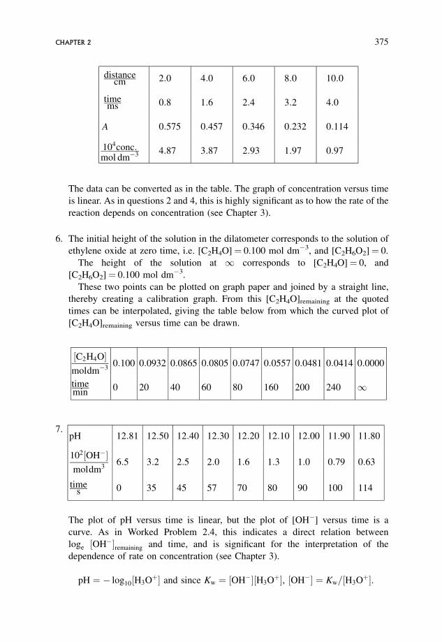
distancecm 2:0 4:0 6:0 8:0 10:0
timems 0:8 1:6 2:4 3:2 4:0
A 0:575 0:457 0:346 0:232 0:114
104conc:mol dm�3 4:87 3:87 2:93 1:97 0:97
The data can be converted as in the table. The graph of concentration versus time
is linear. As in questions 2 and 4, this is highly significant as to how the rate of the
reaction depends on concentration (see Chapter 3).
6. The initial height of the solution in the dilatometer corresponds to the solution of
ethylene oxide at zero time, i.e. [C2H4O]¼ 0.100 mol dm�3, and [C2H6O2]¼ 0.
The height of the solution at 1 corresponds to [C2H4O]¼ 0, and
[C2H6O2]¼ 0.100 mol dm�3.
These two points can be plotted on graph paper and joined by a straight line,
thereby creating a calibration graph. From this [C2H4O]remaining at the quoted
times can be interpolated, giving the table below from which the curved plot of
[C2H4O]remaining versus time can be drawn.
½C2H4O�moldm�3
0:100 0:0932 0:0865 0:0805 0:0747 0:0557 0:0481 0:0414 0:0000
timemin
0 20 40 60 80 160 200 240 1
7.pH 12:81 12:50 12:40 12:30 12:20 12:10 12:00 11:90 11:80
102½OH��moldm3
6:5 3:2 2:5 2:0 1:6 1:3 1:0 0:79 0:63
times 0 35 45 57 70 80 90 100 114
The plot of pH versus time is linear, but the plot of [OH�] versus time is a
curve. As in Worked Problem 2.4, this indicates a direct relation between
loge ½OH��remaining and time, and is significant for the interpretation of the
dependence of rate on concentration (see Chapter 3).
pH ¼ � log10½H3Oþ� and since Kw ¼ ½OH��½H3Oþ�, ½OH�� ¼ Kw=½H3Oþ�.
CHAPTER 2 375
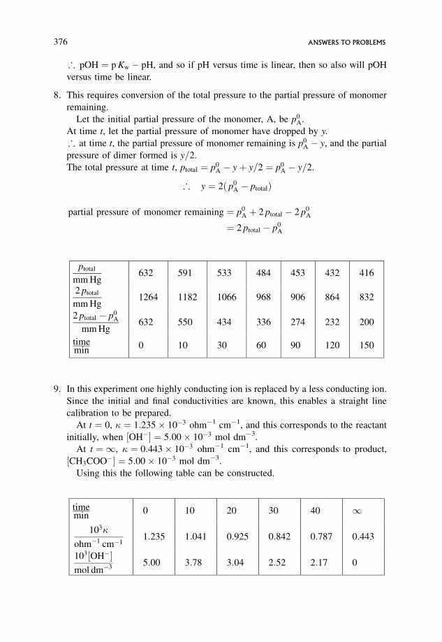
; pOH ¼ p Kw � pH, and so if pH versus time is linear, then so also will pOH
versus time be linear.
8. This requires conversion of the total pressure to the partial pressure of monomer
remaining.
Let the initial partial pressure of the monomer, A, be p0A.
At time t, let the partial pressure of monomer have dropped by y.
; at time t, the partial pressure of monomer remaining is p0A � y, and the partial
pressure of dimer formed is y=2.
The total pressure at time t, ptotal ¼ p0A � yþ y=2 ¼ p0
A � y=2.
; y ¼ 2ð p0A � ptotalÞ
partial pressure of monomer remaining ¼ p0A þ 2 ptotal � 2 p0
A
¼ 2 ptotal � p0A
ptotal
mm Hg632 591 533 484 453 432 416
2 ptotal
mm Hg1264 1182 1066 968 906 864 832
2 ptotal � p0A
mm Hg632 550 434 336 274 232 200
timemin
0 10 30 60 90 120 150
9. In this experiment one highly conducting ion is replaced by a less conducting ion.
Since the initial and final conductivities are known, this enables a straight line
calibration to be prepared.
At t ¼ 0, � ¼ 1:235 10�3 ohm�1 cm�1, and this corresponds to the reactant
initially, when ½OH�� ¼ 5:00 10�3 mol dm�3.
At t ¼ 1, � ¼ 0:443 10�3 ohm�1 cm�1, and this corresponds to product,
½CH3COO�� ¼ 5:00 10�3 mol dm�3.
Using this the following table can be constructed.
timemin
0 10 20 30 40 1
103�
ohm�1 cm�11:235 1:041 0:925 0:842 0:787 0:443
103½OH��mol dm�3
5:00 3:78 3:04 2:52 2:17 0
376 ANSWERS TO PROBLEMS
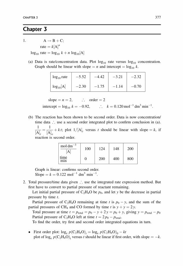
Chapter 3
1. A! Bþ C;
rate ¼ k½A�n
log10 rate ¼ log10 k þ n log10½A�
(a) Data is rate/concentration data. Plot log10 rate versus log10 concentration.
Graph should be linear with slope ¼ n and intercept ¼ log10 k.
log10 rate �5:52 �4:42 �3:21 �2:32
log10½A� �2:30 �1:75 �1:14 �0:70
slope ¼ n ¼ 2; ; order ¼ 2
intercept ¼ log10 k ¼ �0:92; ; k ¼ 0:120 mol�1 dm3 min�1:
(b) The reaction has been shown to be second order. Data is now concentration/
time data ; use a second order integrated plot to confirm conclusion in (a).
1
½A�t¼ 1
½A�oþ k t; plot 1=½A�t versus t should be linear with slope ¼ k, if
reaction is second order.
mol dm�3
½A� 100 124 148 200
timemin
0 200 400 800
Graph is linear: confirms second order.
Slope ¼ k ¼ 0:122 mol�1 dm3 min�1.
2. Total pressure/time data given ; use the integrated rate expression method. But
first have to convert to partial pressure of reactant remaining.
Let initial partial pressure of C2H4O be p0, and let y be the decrease in partial
pressure by time t.
Partial pressure of C2H4O remaining at time t is p0 � y, and the sum of the
partial pressures of CH4 and CO formed by time t is yþ y ¼ 2 y.
Total pressure at time t ¼ ptotal ¼ p0 � yþ 2 y ¼ p0 þ y, giving y ¼ ptotal � p0
Partial pressure of C2H4O left at time t ¼ 2 p0 � ptotal.
To find the order, try first and second order integrated equations in turn.
� First order plot: loge pðC2H4OÞt ¼ loge pðC2H4OÞ0 � kt
plot of loge pðC2H4OÞt versus t should be linear if first order, with slope ¼ �k.
CHAPTER 3 377
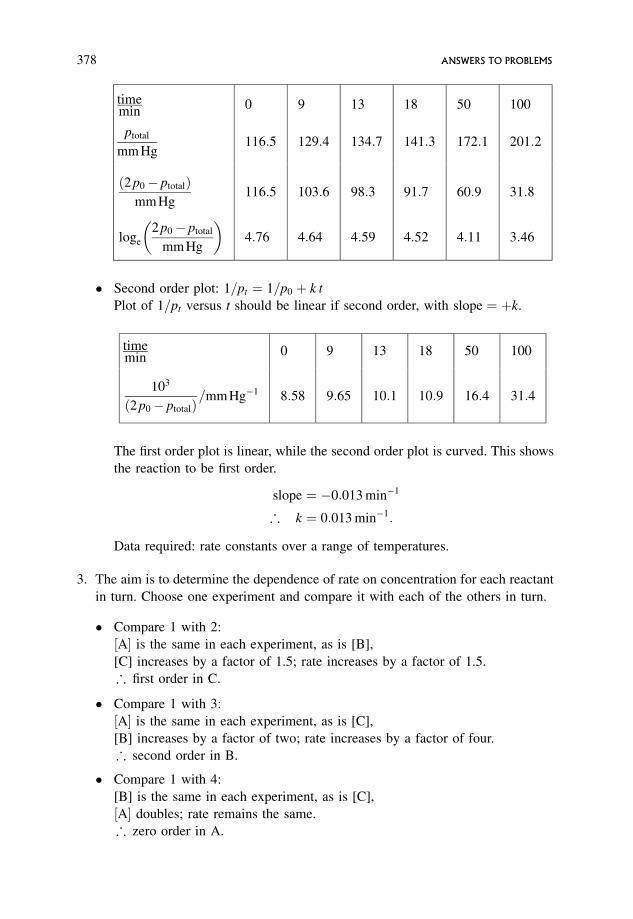
timemin
0 9 13 18 50 100
ptotal
mmHg116:5 129:4 134:7 141:3 172:1 201:2
ð2p0� ptotalÞmmHg
116:5 103:6 98:3 91:7 60:9 31:8
loge
2p0� ptotal
mmHg
� �4:76 4:64 4:59 4:52 4:11 3:46
� Second order plot: 1=pt ¼ 1=p0 þ k t
Plot of 1=pt versus t should be linear if second order, with slope ¼ þk.
timemin
0 9 13 18 50 100
103
ð2p0� ptotalÞ=mmHg�1 8:58 9:65 10:1 10:9 16:4 31:4
The first order plot is linear, while the second order plot is curved. This shows
the reaction to be first order.
slope ¼ �0:013 min�1
; k ¼ 0:013 min�1:
Data required: rate constants over a range of temperatures.
3. The aim is to determine the dependence of rate on concentration for each reactant
in turn. Choose one experiment and compare it with each of the others in turn.
� Compare 1 with 2:
½A� is the same in each experiment, as is [B],
[C] increases by a factor of 1.5; rate increases by a factor of 1.5.
; first order in C.
� Compare 1 with 3:
½A� is the same in each experiment, as is [C],
[B] increases by a factor of two; rate increases by a factor of four.
; second order in B.
� Compare 1 with 4:
[B] is the same in each experiment, as is [C],
½A� doubles; rate remains the same.
; zero order in A.
378 ANSWERS TO PROBLEMS
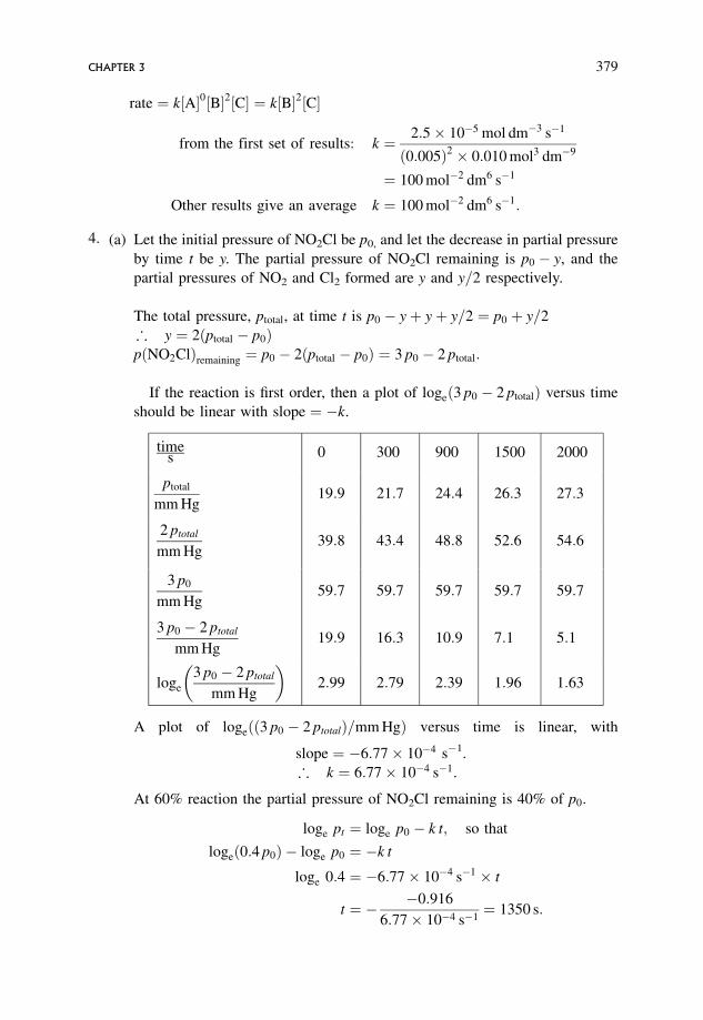
rate ¼ k½A�0½B�2½C� ¼ k½B�2½C�
from the first set of results: k ¼ 2:5 10�5 mol dm�3 s�1
ð0:005Þ2 0:010 mol3 dm�9
¼ 100 mol�2 dm6 s�1
Other results give an average k ¼ 100 mol�2 dm6 s�1:
4. (a) Let the initial pressure of NO2Cl be p0, and let the decrease in partial pressure
by time t be y. The partial pressure of NO2Cl remaining is p0 � y, and the
partial pressures of NO2 and Cl2 formed are y and y=2 respectively.
The total pressure, ptotal, at time t is p0 � yþ yþ y=2 ¼ p0 þ y=2
; y ¼ 2ðptotal � p0ÞpðNO2ClÞremaining ¼ p0 � 2ðptotal � p0Þ ¼ 3 p0 � 2 ptotal:
If the reaction is first order, then a plot of logeð3 p0 � 2 ptotalÞ versus time
should be linear with slope ¼ �k.
times 0 300 900 1500 2000
ptotal
mm Hg19:9 21:7 24:4 26:3 27:3
2 ptotal
mm Hg39:8 43:4 48:8 52:6 54:6
3 p0
mm Hg59:7 59:7 59:7 59:7 59:7
3 p0 � 2 ptotal
mm Hg19:9 16:3 10:9 7:1 5:1
loge
3 p0 � 2 ptotal
mm Hg
� �2:99 2:79 2:39 1:96 1:63
A plot of loge ð3 p0 � 2 ptotalÞ=mm Hgð Þ versus time is linear, with
slope ¼ �6:77 10�4 s�1.
; k ¼ 6:77 10�4 s�1.
At 60% reaction the partial pressure of NO2Cl remaining is 40% of p0.
loge pt ¼ loge p0 � k t; so that
logeð0:4 p0Þ � loge p0 ¼ �k t
loge 0:4 ¼ �6:77 10�4 s�1 t
t ¼ � �0:916
6:77 10�4 s�1¼ 1350 s:
CHAPTER 3 379
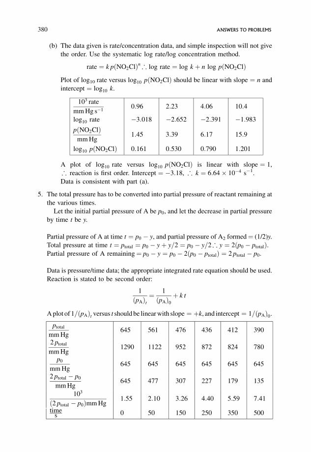
(b) The data given is rate/concentration data, and simple inspection will not give
the order. Use the systematic log rate/log concentration method.
rate ¼ k pðNO2ClÞn; log rate ¼ log k þ n log pðNO2ClÞ
Plot of log10 rate versus log10 pðNO2ClÞ should be linear with slope ¼ n and
intercept ¼ log10 k.
103 rate
mm Hg s�10:96 2:23 4:06 10:4
log10 rate �3:018 �2:652 �2:391 �1:983
pðNO2ClÞmm Hg
1:45 3:39 6:17 15:9
log10 pðNO2ClÞ 0:161 0:530 0:790 1:201
A plot of log10 rate versus log10 pðNO2ClÞ is linear with slope ¼ 1,
; reaction is first order. Intercept ¼ �3:18, ; k ¼ 6:64 10�4 s�1.
Data is consistent with part (a).
5. The total pressure has to be converted into partial pressure of reactant remaining at
the various times.
Let the initial partial pressure of A be p0, and let the decrease in partial pressure
by time t be y.
Partial pressure of A at time t ¼ p0 � y, and partial pressure of A2 formed¼ (1/2)y.
Total pressure at time t ¼ ptotal ¼ p0 � yþ y=2 ¼ p0 � y=2; y ¼ 2ðp0 � ptotalÞ.Partial pressure of A remaining¼ p0 � y ¼ p0 � 2ðp0 � ptotalÞ ¼ 2 ptotal � p0.
Data is pressure/time data; the appropriate integrated rate equation should be used.
Reaction is stated to be second order:
1
ðpAÞt¼ 1
ðpAÞ0þ k t
A plot of 1=ðpAÞt versus t should be linear with slope ¼ þk, and intercept ¼ 1=ðpAÞ0.
ptotal
mm Hg645 561 476 436 412 390
2 ptotal
mm Hg1290 1122 952 872 824 780
p0
mm Hg645 645 645 645 645 645
2 ptotal � p0
mm Hg645 477 307 227 179 135
103
ð2 ptotal � p0Þmm Hg1:55 2:10 3:26 4:40 5:59 7:41
times 0 50 150 250 350 500
380 ANSWERS TO PROBLEMS
Plot is linear, confirming reaction to be second order with
slope ¼ k ¼ 1:17 10�5ðmm HgÞ�1s�1.
At the first half-life pA ¼ 1=2 p0
1=ðpAÞt ¼ 1=ðpAÞ0 þ k t gives
1
ð1=2ÞðpAÞ0¼ 1
ðpAÞ0þ k t1=2 ;
1
ðpAÞ0¼ k t1=2
and
t1=2 ¼1
kðpAÞ0¼ 1
1:17 10�5ðmm HgÞ�1s�1 645 mm Hg
¼ 132 s
The first half-life is 132 s.
At the second half-life, pA ¼ ð1=4Þ p0, and the time to reach this partial
pressure ¼ 3=kðpAÞ0 ¼ 397 s.
The second half-life is the difference in time for the partial pressure of A to
decrease to (1/4) p0 from (1/2) p0 ¼ (397� 132) s¼ 265 s.
Second half-life > first half-life, confirming the second order behaviour.
6. Orders with respect to two reactants are required. Look to see whether there are
any experiments where one substance is at the same pressure, while the pressure
of the other reactant is altered, i.e. look for pseudo-order conditions.
� In experiments 3 and 1, p(N2O) initially is the same while the initial p(Cl2) is
altered.
p(Cl2) increases by a factor of four; rate increases by a factor of two.
rate / ðpressureÞn, ; 2 ¼ 4n and n ¼ 1=2. Order with respect to Cl2 is 1/2.
� In experiments 2 and 1, p(Cl2) initially is the same while the initial p(N2O) is
altered.
p(N2O) increases by a factor of two; rate also increases by a factor of two.
Reaction is first order with respect to N2O.
Rate ¼ k p(N2O)p(Cl2)1/2 with overall order¼ 3/2.
7. Data given is concentration/time data, ; use the integrated rate equation to
confirm first order kinetics.
The reaction is catalysed by acids, but during the experiment quoted [acid]
remains constant, and reaction is being carried out under pseudo-order conditions.
Toluene is both a reactant and the solvent, and so the toluene will always be in
excess, and again reaction is carried out under pseudo-order conditions.
rate ¼ k½C6H5CH3�m½catalyst�n½Cl2�p
Since during any given experiment, [C6H5CH3] and [catalyst] are held constant,
and the order with respect to Cl2 is stated to be first, then
rate ¼ k0½Cl2�loge½Cl2�t ¼ loge½Cl2�0 � k0t:
CHAPTER 3 381
Data given is [Cl2] remaining at time t ; no need to carry out any stoichiometric
conversion.
Plot of loge½Cl2�t versus t should be linear with slope ¼ �k0.
½Cl2�mol dm�3
0:0775 0:0565 0:0410 0:0265 0:0175
timemin
0 3 6 10 14
loge½Cl2� �2:557 �2:874 �3:194 �3:631 �4:046
Plot is linear, confirming reaction to be first order, with slope ¼ �10:710�2 min�1, and k0 ¼ 10:7 10�2 min�1.
Part (b) gives values of the pseudo-first order rate constant for a series of
[catalyst]. For any given [catalyst],
rate ¼ k0½Cl2� where k0 is the pseudo-first order rate constant found in part (a),
and k0 ¼ k00½catalyst�n where k00 ¼ k[C6H5CH3]m
log10 k0 ¼ log10 k00 þ n log10 ½catalyst�
; plot of log10 k0 versus log10 [catalyst] should be linear with slope ¼ n and
intercept ¼ log10 k00.From part (a) k0 ¼ 10:7 10�2 min�1 when [catalyst]¼ 0.117 mol dm�3.
log10½catalyst� �1:301 �1:125 �1:000 �0:932 �0:815 �0:699
log10 k0 �1:556 �1:276 �1:046 �0:971 �0:764 �0:569
Plot is linear with slope¼1:6, and it is likely that the order is 3/2, i.e. 1.5, with
respect to catalyst.
Chapter 4
1. � Atom has three translations.
Non-linear molecule has three translations, three rotations, and ð3N � 6Þvibrations.
Total for reactants: six translations, three rotations, ð3N � 6Þ vibrations.
Non-linear activated complex has three translations, three rotations, one
internal translation and ð3ðN þ 1Þ � 7Þ vibrations, i.e ð3 N � 4Þ vibrations.
382 ANSWERS TO PROBLEMS

On activation: lose three translations; gain two vibrations and one internal
translation.
� Linear molecule has three translations, two rotations and ð3 NA � 5Þ vibrations.
Non-linear molecule has three translations, three rotations and ð3 NB � 6Þvibrations.
Total for reactants: six translations, five rotations and ð3 NA þ 3 NB � 11Þvibrations.
Non-linear activated complex has three translations, three rotations, one
internal translation and ð3 NA þ 3 NB � 7Þ vibrations.
On activation: lose three translations and two rotations; gain four vibrations
and one internal translation.
� Two linear molecules have six translations, four rotations and ð3 NA þ 3 NB�10Þ vibrations.
Linear activated complex has three translations, two rotations, one internal
translation and ð3 NA þ 3 NB � 6Þ vibrations.
On activation: lose three translations and two rotations; gain four vibrations
and one internal translation.
� Two linear molecules have six translations, four rotations and ð3 NA þ 3 NB�10Þ vibrations.
Non-linear activated complex has three translations, three rotations, one
internal translation and ð3 NA þ 3 NB � 7Þ vibrations.
On activation: lose three translations and one rotation; gain three vibrations
and one internal translation.
� Non-linear molecule has three translations, three rotations and ð3 N � 6Þ vibrations.
Non-linear activated complex has three translations, three rotations, one
internal translation and ð3 N � 7Þ vibrations.
On activation: lose one vibration; gain one internal translation.
2. The temperature dependence of kobs will give values to �H 6¼�and �S6¼�.
k ¼ � k T
hK 6¼ � ¼ � k T
hexp
��H 6¼ �
RT
� �exp
þ� S6¼ �
R
!
loge
k
T¼ loge
� k
h��H 6¼ �
RTþ� S6¼ �
R
A plot of logeðk=TÞ versus 1=T should be linear with slope ¼ ��H 6¼ �=R. The
intercept should be loge ð� k=hÞ þ� S6¼ �=R. But, because this would involve a
ridiculous extrapolation, � S6¼ � will have to be calculated.
�G� for reactions in solution depends on pressure, in contrast to gas phase
reactions, for which �G� is independent of pressure.
CHAPTER 4 383
One of the key equations of thermodynamics is
d G ¼ V d p� S d T
At constant T, d T ¼ 0 and S d T ¼ 0, giving
d G ¼ V d p
ðp2
p1
d G ¼ðp2
p1
V d p
For an ideal gas p V ¼ n RT givingðp2
p1
d G ¼ n RT
ðp2
p1
d p
p
from which
Gp2� Gp1
¼ n RT loge
p2
p1
and, if the standard state is 1 atm (more recently 1 bar), then � ¼ �� þ RT loge p,
where �� is a constant dependent on T and independent of p.
1 bar ¼ 1:000 � � � 105 N m�2ðPaÞ1 atm ¼ 1:01325 105 N m�2ðPaÞ
�G� is a combination of �� values for products and reactants, and so is also
independent of pressure.
For a substance in solution, the analogous equation for the ideal case is
� ¼ �� þ RT loge c, where �� is a constant dependent on T and also on pressure.
Correspondingly, �G� is a constant dependent on both T and pressure.
3. Br� þ H2 ! HBr þ H�
Br�: atom with three translations
H2: two atoms, linear molecule with three translations, two rotations and one
vibration.
Activated complex: three atoms, linear, three translations, two rotations, one
internal translation and three vibrations.
On activation: lose three translations, and gain two vibrations.
� S6¼ � ¼ �ð3 50Þ J mol�1 K�1 þ ð2 10Þ J mol�1 K�1
¼ �130 J mol�1 K�1
CH�3 þ H2 ! CH4 þ H�
CH�3: four atoms, non-linear molecule with three translations, three rotations and
six vibrations.
384 ANSWERS TO PROBLEMS
H2: two atoms, linear molecule with three translations, two rotations and one
vibration.
Total for reactants: six translations, five rotations and seven vibrations.
Activated complex: six atoms, non-linear, three translations, three rotations, one
internal translation and 11 vibrations.
On activation: lose three translations, lose two rotations and gain four
vibrations.
� S6¼ � ¼ �ð3 50Þ J mol�1 K�1 � ð2 40Þ J mol�1 K�1 þ ð4 10Þ J mol�1 K�1
¼ �190 J mol�1K�1:
F2 þ ClO�2 ! FClO2 þ F�
F2: two atoms, linear molecule with three translations, two rotations and one
vibration.
ClO2: three atoms, non-linear molecule with three translations, three rotations and
three vibrations.
Total for reactants: six translations, five rotations and four vibrations.
Activated complex: five atoms, non-linear, three translations, three rotations, one
internal translation and eight vibrations.
On activation: lose three translations, lose two rotations and gain four
vibrations.
� S6¼ � ¼ �ð3 50Þ J mol�1 K�1 � ð2 40Þ J mol�1 K�1 þ ð4 10Þ J mol�1 K�1
¼ �190 J mol�1 K�1:
C4H6 þ C2H4 ! cyclo-C6H10
C4H6: 10 atoms, non-linear molecule with three translations, three rotations and
24 vibrations.
C2H4: six atoms, non-linear molecule with three translations, three rotations and
12 vibrations.
Total for reactants: six translations, six rotations and 36 vibrations.
Activated complex: 16 atoms, non-linear, three translations, three rotations, one
internal translation and 41 vibrations.
On activation: lose three translations, lose three rotations and gain five
vibrations.
� S6¼ � ¼ �ð3 50Þ J mol�1 K�1 � ð3 40Þ J mol�1 K�1 þ ð5 10Þ J mol�1 K�1
¼ �220 J mol�1 K�1:
Note the following.
� As the complexity of the reactants increases, the entropy loss becomes greater
and consequently the A factor will decrease.
CHAPTER 4 385
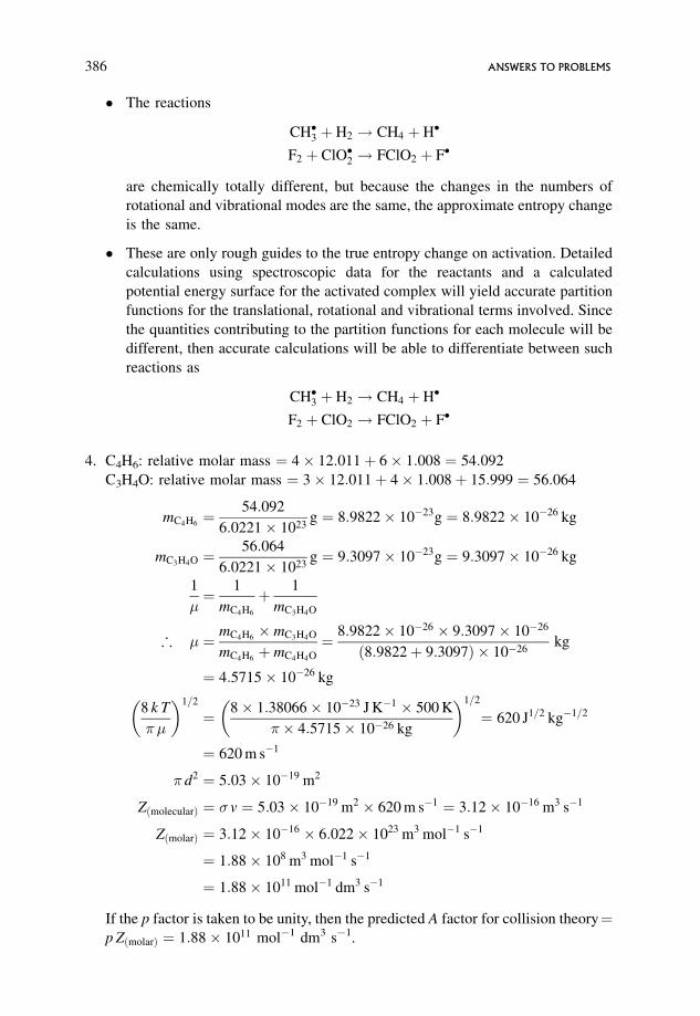
� The reactions
CH�3 þ H2 ! CH4 þ H�
F2 þ ClO�2 ! FClO2 þ F�
are chemically totally different, but because the changes in the numbers of
rotational and vibrational modes are the same, the approximate entropy change
is the same.
� These are only rough guides to the true entropy change on activation. Detailed
calculations using spectroscopic data for the reactants and a calculated
potential energy surface for the activated complex will yield accurate partition
functions for the translational, rotational and vibrational terms involved. Since
the quantities contributing to the partition functions for each molecule will be
different, then accurate calculations will be able to differentiate between such
reactions as
CH�3 þ H2 ! CH4 þ H�
F2 þ ClO2 ! FClO2 þ F�
4. C4H6: relative molar mass ¼ 4 12:011þ 6 1:008 ¼ 54:092
C3H4O: relative molar mass ¼ 3 12:011þ 4 1:008þ 15:999 ¼ 56:064
mC4H6¼ 54:092
6:0221 1023g ¼ 8:9822 10�23g ¼ 8:9822 10�26 kg
mC3H4O ¼56:064
6:0221 1023g ¼ 9:3097 10�23g ¼ 9:3097 10�26 kg
1
�¼ 1
mC4H6
þ 1
mC3H4O
; � ¼ mC4H6 mC3H4O
mC4H6þ mC4H4O
¼ 8:9822 10�26 9:3097 10�26
ð8:9822þ 9:3097Þ 10�26kg
¼ 4:5715 10�26 kg
8 k T
�
� �1=2
¼ 8 1:38066 10�23 J K�1 500 K
4:5715 10�26 kg
� �1=2
¼ 620 J1=2 kg�1=2
¼ 620 m s�1
d2 ¼ 5:03 10�19 m2
ZðmolecularÞ ¼ v ¼ 5:03 10�19 m2 620 m s�1 ¼ 3:12 10�16 m3 s�1
ZðmolarÞ ¼ 3:12 10�16 6:022 1023 m3 mol�1 s�1
¼ 1:88 108 m3 mol�1 s�1
¼ 1:88 1011 mol�1 dm3 s�1
If the p factor is taken to be unity, then the predicted A factor for collision theory¼p ZðmolarÞ ¼ 1:88 1011 mol�1 dm3 s�1.
386 ANSWERS TO PROBLEMS

Entropies of activation.
C4H6: 10 atoms, non-linear ; three translations, three rotations and 24 vibrations
C3H4O: eight atoms, non-linear; three translations, three rotations and 18 vibrations
activated complex: 18 atoms ; three translations, three rotations, one internal
translation and 47 vibrations
; on forming the activated complex
lose three translations and three rotations,
gain five vibrations.
� S6¼ � � �ð3 40Þ � ð3 25Þ þ ð5 10Þ J mol�1 K�1
¼ �145 J mol�1 K�1
p corresponds to exp ð� S 6¼ �=RÞ ¼ exp �145=8:3145ð Þ ¼ 2:7 10�8
A ¼ e2� k T
hexp
� S 6¼ �
R
� �¼ e211:3806610�23 J K�1 500 K
6:626110�34 J s2:710�8
¼ 2:1 106 mol�1 dm3 s�1
(The factor e2 takes account of the difference between the Arrhenius equation given in
terms of the experimental activation energy, and that in terms of the enthalpy of
activation.)
collision theory A factor ¼ 1:88 1011 mol�1 dm3 s�1
approximate transition state theory A factor ¼ 2:1 106 mol�1 dm3 s�1
experimental A factor ¼ 1:6 106 mol�1 dm3 s�1
There is a large discrepancy between the experimental and the collision theory
values, demonstrating the inadequacy of collision theory. There is excellent agreement
between the experimental and transition state theory values, though, in part, the very
close agreement is merely a reflection of the particular typical magnitudes taken for
the entropy contributions. However, even taking upper and lower limits to these
contributions still gives magnitudes for the A factor which are much closer to the
experimental A factor than the collision theory value.
5. The Lindemann mechanism gives
k1stobs ¼
k1 k2½A�k�1½A� þ k2
1
k1stobs
¼ k�1
k1 k2
þ 1
k1½A�If k1, k�1 and k2 are all constants, then the graph of 1=k1st
obs versus 1=½A� should be
linear with slope ¼ 1=k1 and intercept ¼ k�1=k1k2.
Using the first set of data
10�3 1
½A�mol�1 dm3
100 67 50 25
1
k1stobs=s�1
3:00 2:56 2:35 2:02
CHAPTER 4 387
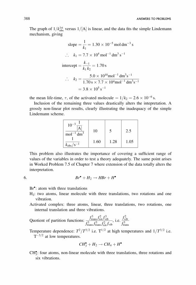
The graph of 1=k1stobs versus 1=½A� is linear, and the data fits the simple Lindemann
mechanism, giving
slope ¼ 1
k1
¼ 1:30 10�5 mol dm�3 s
; k1 ¼ 7:7 104 mol�1 dm3 s�1
intercept ¼ k�1
k1 k2
¼ 1:70 s
; k2 ¼5:0 1010mol�1 dm3s�1
1:70 s 7:7 104mol�1 dm3s�1
¼ 3:8 105 s�1
the mean life-time, � , of the activated molecule ¼ 1=k2 ¼ 2:6 10�6 s.
Inclusion of the remaining three values drastically alters the intepretation. A
grossly non-linear plot results, clearly illustrating the inadequacy of the simple
Lindemann scheme.
10�3 1
½A�mol�1 dm3
10 5 2:5
1
kobs=s�11:60 1:28 1:05
This problem also illustrates the importance of covering a sufficient range of
values of the variables in order to test a theory adequately. The same point arises
in Worked Problem 7.5 of Chapter 7 where extension of the data totally alters the
interpretation.
6. Br� þ H2 ! HBr þ H�
Br�: atom with three translations
H2: two atoms, linear molecule with three translations, two rotations and one
vibration.
Activated complex: three atoms, linear, three translations, two rotations, one
internal translation and three vibrations.
Quotient of partition functions:f 3trans f 2
rot f 3vib
f 3trans f 3
trans f 2rot fvib
, i.e.f 2vib
f 3trans
Temperature dependence: T2=T3=2 i.e. T1=2 at high temperatures and 1=T3=2 i.e.
T�3=2 at low temperatures.
CH�3 þ H2 ! CH4 þ H�
CH�3: four atoms, non-linear molecule with three translations, three rotations and
six vibrations.
388 ANSWERS TO PROBLEMS
H2: two atoms, linear molecule with three translations, two rotations and one
vibration.
Activated complex: six atoms, non-linear, three translations, three rotations, one
internal translation and 11 vibrations.
Quotient of partition functions:f 3trans f 3
rot f 11vib
f 3trans f 3
rot f 6vib f 3
trans f 2rot fvib
i.e.f 4vib
f 3trans f 2
rot
Temperature dependence:T4
T3=2Ti.e. T 3=2 at high temperatures, and
1
T3=2Ti.e.
T�5=2 at low temperatures.
F2 þ ClO�2 ! FClO2 þ F�
F2: two atoms, linear molecule with three translations, two rotations and one
vibration.
ClO2: three atoms, non-linear molecule with three translations, three rotations and
three vibrations.
Activated complex: five atoms, non-linear, three translations, three rotations, one
internal translation and eight vibrations.
Quotient of partition functions:f 3trans f 3
rot f 8vib
f 3trans f 2
rot fvib f 3trans f 3
rot f 3vib
i.e.f 4vib
f 3trans f 2
rot
Temperature dependence:T4
T3=2Ti.e. T 3=2 at high temperatures, and
1
T3=2Ti.e.
T�5=2 at low temperatures.
C4H6 þ C2H4 ! cyclo-C6H10
C4H6: 10 atoms, non-linear molecule with three translations, three rotations and
24 vibrations.
C2H4: six atoms, non-linear molecule with three translations, three rotations and
12 vibrations.
Activated complex: 16 atoms, non-linear, three translations, three rotations, one
internal translation and 41 vibrations.
Quotient of partition functions:f 3trans f 3
rot f 41vib
f 3trans f 3
rot f 24vib f 3
trans f 3rot f 12
vib
i.e.f 5vib
f 3trans f 3
rot
Temperature dependence:T5
T3=2T3=2i.e. T2 at high temperatures, and
1
T3=2T3=2i.e.
T�3 at low temperatures.
7. � cyclopropane! propene
The � S6¼ � and � S� values are similar: reaction is 1! 1 and so the entropy
change is not associated with a change in the number of molecules. The
activated complex resembles the product and so bond breaking and making is
well developed in the activated complex. On isomerization there is release of
the strain in the three-membered ring.
CHAPTER 4 389
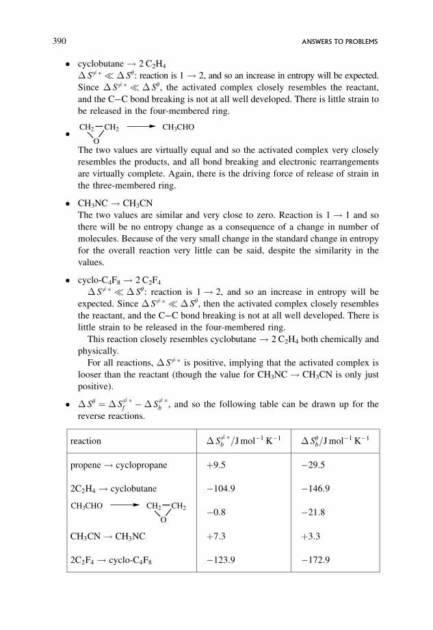
� cyclobutane! 2 C2H4
� S6¼ � � � S�: reaction is 1! 2, and so an increase in entropy will be expected.
Since � S6¼ � � � S�, the activated complex closely resembles the reactant,
and the C��C bond breaking is not at all well developed. There is little strain to
be released in the four-membered ring.
�CH2
O
CH2 CH3CHO
The two values are virtually equal and so the activated complex very closely
resembles the products, and all bond breaking and electronic rearrangements
are virtually complete. Again, there is the driving force of release of strain in
the three-membered ring.
� CH3NC! CH3CN
The two values are similar and very close to zero. Reaction is 1! 1 and so
there will be no entropy change as a consequence of a change in number of
molecules. Because of the very small change in the standard change in entropy
for the overall reaction very little can be said, despite the similarity in the
values.
� cyclo-C4F8! 2 C2F4
� S6¼ � � � S�: reaction is 1! 2, and so an increase in entropy will be
expected. Since � S 6¼ � � � S�, then the activated complex closely resembles
the reactant, and the C��C bond breaking is not at all well developed. There is
little strain to be released in the four-membered ring.
This reaction closely resembles cyclobutane! 2 C2H4 both chemically and
physically.
For all reactions, � S6¼ � is positive, implying that the activated complex is
looser than the reactant (though the value for CH3NC! CH3CN is only just
positive).
� � S� ¼ � S6¼ �f �� S
6¼ �b , and so the following table can be drawn up for the
reverse reactions.
reaction � S6¼ �b =J mol�1 K�1 � S�b=J mol�1 K�1
propene! cyclopropane þ9:5 �29:5
2C2H4 ! cyclobutane �104:9 �146:9
CH2
O
CH2CH3CHO�0:8 �21:8
CH3CN! CH3NC þ7:3 þ3:3
2C2F4 ! cyclo-C4F8 �123:9 �172:9
390 ANSWERS TO PROBLEMS
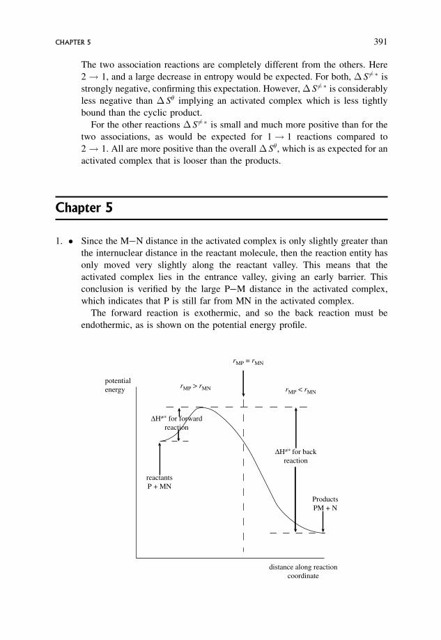
The two association reactions are completely different from the others. Here
2! 1, and a large decrease in entropy would be expected. For both, � S 6¼ � is
strongly negative, confirming this expectation. However, � S6¼ � is considerably
less negative than � S� implying an activated complex which is less tightly
bound than the cyclic product.
For the other reactions � S6¼ � is small and much more positive than for the
two associations, as would be expected for 1! 1 reactions compared to
2! 1. All are more positive than the overall � S�, which is as expected for an
activated complex that is looser than the products.
Chapter 5
1. � Since the M��N distance in the activated complex is only slightly greater than
the internuclear distance in the reactant molecule, then the reaction entity has
only moved very slightly along the reactant valley. This means that the
activated complex lies in the entrance valley, giving an early barrier. This
conclusion is verified by the large P��M distance in the activated complex,
which indicates that P is still far from MN in the activated complex.
The forward reaction is exothermic, and so the back reaction must be
endothermic, as is shown on the potential energy profile.
potentialenergy rMP > rMN
rMP = rMN
rMP < rMN
∆H≠∗ for backreaction
ProductsPM + N
distance along reactioncoordinate
reactantsP + MN
∆H≠∗ for forwardreaction
CHAPTER 5 391
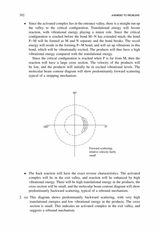
� Since the activated complex lies in the entrance valley, there is a straight run up
the valley to the critical configuration. Translational energy will favour
reaction, with vibrational energy playing a minor role. Since the critical
configuration is reached before the bond M��N has extended much, the bond
P��M will be formed as M and N separate and the bond breaks. The recoil
energy will reside in the forming P��M bond, and will set up vibrations in this
bond, which will be vibrationally excited. The products will thus have a high
vibrational energy compared with the translational energy.
Since the critical configuration is reached when P is far from M, then the
reaction will have a large cross section. The velocity of the products will
be low, and the products will initially be in excited vibrational levels. The
molecular beam contour diagram will show predominantly forward scattering
typical of a stripping mechanism.
� The back reaction will have the exact reverse characteristics. The activated
complex will lie in the exit valley, and reaction will be enhanced by high
vibrational energy. There will be high translational energy in the products, the
cross section will be small, and the molecular beam contour diagram will show
predominantly backward scattering, typical of a rebound mechanism.
2. (a) This diagram shows predominantly backward scattering, with very high
translational energies and low vibrational energy in the products. The cross
section is small. This indicates an activated complex in the exit valley, and
suggests a rebound mechanism.
0°180°
90°
Forward scattering;relative velocity fairlysmall
392 ANSWERS TO PROBLEMS
(b) This diagram suggests that the reaction occurs via a ‘cutting the corner’
trajectory where the usual minimum energy path is not followed.
3. As the vibrational ladder is climbed, i.e. v the vibrational quantum number
increases, the vibrational energy increases. The question thus states that reaction
becomes faster as the vibrational energy increases.
This means that vibrational energy favours reaction, from which it can be
inferred that the activated complex lies in the exit valley, and that there is a
late barrier. This is a rebound mechanism where the reactants have to get very
close together before reaction can occur.
4. (a) If the cross section is large, then reaction can occur when the reactants
are far apart. This is a stripping mechanism where the activated complex
lies in the entrance valley, there is an early barrier and products will
separate with predominantly vibrational energy. The reaction will be
favoured by high translational energies. In a stripping mechanism, the Ca
will pull off the O from the NO2 at a distance, and continue on with only a
small deflection from the original trajectory. This implies that there must be
strong forces of interaction between the reactant molecules for this to be
possible.
(b) In contrast to the above reaction, a small cross section implies that reaction
can only occur at small distances apart. This is typical of a rebound
mechanism, where the activated complex occurs in the exit valley, where
there is a late barrier and products will separate with predominantly high
translational energy. The reaction will be favoured by high vibrational
energies. In a rebound mechanism the CH�3 will only react with the Br2
when they are almost in contact, and on rebound it will fly off in a backwards
direction, so that there is backwards scattering of products on the molecular
beam contour diagram. Since reaction can only occur when the reactants are
close together, the forces of interaction must be relatively weak.
(c) In this reaction the molecular contour diagram shows both forward and
backward scattering. This is typical of a reaction with a collision complex
where many rotations, and perhaps several vibrations occur, before the
products separate. The directions in which the product molecules separate
in this situation will be random, and a fairly symmetrical scattering pattern
will result.
(d) If the products are predominantly in the ground vibrational state this implies
that the energy of the products is predominantly translational, characteristic of
a rebound mechanism with a late barrier where the activated complex is in the
exit valley. The other characteristics will be as in (b) above.
(e) The cross section is related to the rate constant for the reaction. The larger the
cross section the greater will be the rate constant. The data given states that
CHAPTER 5 393
the rate constant for reaction is greater if the reactant is vibrationally
excited. This is a characteristic of a rebound mechanism where the
activated complex is in the exit valley and the potential energy profile has a
late barrier. For the other characteristics of a rebound mechanism, see (b) and
(d) above.
5. (a) The radii are 80 pm and 190 pm, so that when the reactant molecules are just
touching the centres of the molecules are 270 pm apart. This would
correspond to a cross section¼ d2, where d ¼ 270 pm.
Cross section corresponding to just touching¼ ð270Þ2 pm2 ¼ 0:23nm2.
Observed cross section¼ 0:20nm2.
Since these two cross sections have similar magnitudes, this would correspond
to a rebound mechanism where the two molecules have to come very close
together before reaction will occur. The activated complex thus lies in the exit
valley and the potential energy profile has a late barrier.
(b) If the mechanism is indeed a rebound mechanism then vibrational energy in
the reactants will favour reaction, and the products will have predominantly
translational energy. This conclusion can be confirmed by the information
given.
translational energy¼ 42:5kJmol�1 ¼ 42:5 103
6:022 1023J¼ 7:06 10�20 J
vibrational energy¼ ðvþ 1=2Þh�0
The product molecule is predominantly in the ground vibrational state, i.e.
v¼ 0.
vibrational energy¼ 1=2 6:626 10�34 J s 3 1013 s�1
¼ 0:994 10�20 J
;translational energy
vibrational energy¼ 7:06 10�20 J
0:994 10�20 J¼ 7:1
Hence the predominant energy in the products is translational, which confirms
the conclusions from the cross sections.
Reaction is a rebound mechanism, with the critical configuration in the exit
valley.
(c) In a rebound mechanism the reactants have to collide head on, and in doing so
the products rebound backwards in a direction opposite to the original line of
approach of the colliding molecules. The molecular beam contour diagram
will show backward scattering.
(d) The potential energy contour diagram and profile are shown in next page.
394 ANSWERS TO PROBLEMS
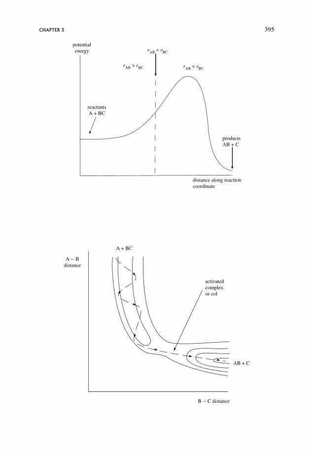
potentialenergy
rAB > rBC
rAB = rBC
rAB < rBC
productsAB + C
distance along reactioncoordinate
reactantsA + BC
activated complexor col
A + BC
AB + C
B -- C distance
A -- Bdistance
CHAPTER 5 395
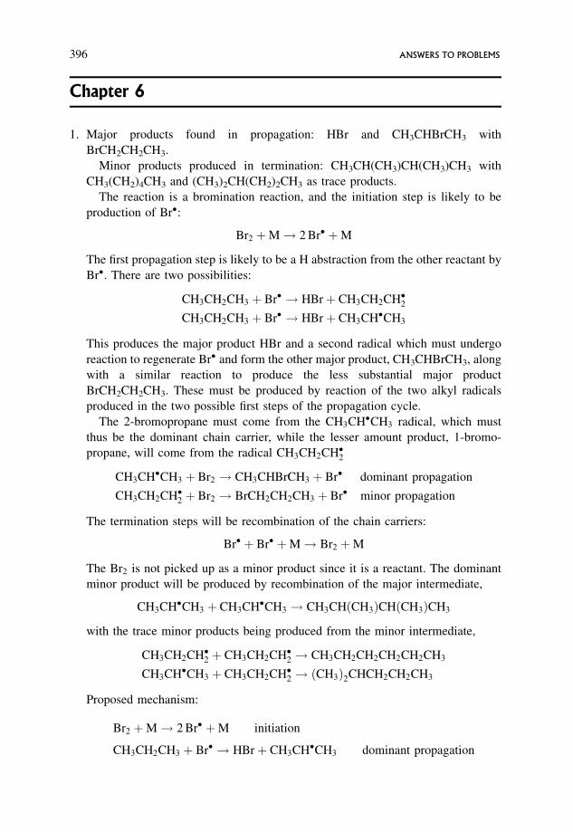
Chapter 6
1. Major products found in propagation: HBr and CH3CHBrCH3 with
BrCH2CH2CH3.
Minor products produced in termination: CH3CH(CH3)CH(CH3)CH3 with
CH3(CH2)4CH3 and (CH3)2CH(CH2)2CH3 as trace products.
The reaction is a bromination reaction, and the initiation step is likely to be
production of Br�:
Br2 þM! 2 Br� þM
The first propagation step is likely to be a H abstraction from the other reactant by
Br�. There are two possibilities:
CH3CH2CH3 þ Br� ! HBrþ CH3CH2CH�2CH3CH2CH3 þ Br� ! HBrþ CH3CH�CH3
This produces the major product HBr and a second radical which must undergo
reaction to regenerate Br� and form the other major product, CH3CHBrCH3, along
with a similar reaction to produce the less substantial major product
BrCH2CH2CH3. These must be produced by reaction of the two alkyl radicals
produced in the two possible first steps of the propagation cycle.
The 2-bromopropane must come from the CH3CH�CH3 radical, which must
thus be the dominant chain carrier, while the lesser amount product, 1-bromo-
propane, will come from the radical CH3CH2CH�2
CH3CH�CH3 þ Br2 ! CH3CHBrCH3 þ Br� dominant propagation
CH3CH2CH�2 þ Br2 ! BrCH2CH2CH3 þ Br� minor propagation
The termination steps will be recombination of the chain carriers:
Br� þ Br� þM! Br2 þM
The Br2 is not picked up as a minor product since it is a reactant. The dominant
minor product will be produced by recombination of the major intermediate,
CH3CH�CH3 þ CH3CH�CH3 ! CH3CHðCH3ÞCHðCH3ÞCH3
with the trace minor products being produced from the minor intermediate,
CH3CH2CH�2 þ CH3CH2CH�2 ! CH3CH2CH2CH2CH2CH3
CH3CH�CH3 þ CH3CH2CH�2 ! ðCH3Þ2CHCH2CH2CH3
Proposed mechanism:
Br2 þM! 2 Br� þM initiation
CH3CH2CH3 þ Br� ! HBrþ CH3CH�CH3 dominant propagation
396 ANSWERS TO PROBLEMS
CH3CH�CH3 þ Br2 ! CH3CHBrCH3 þ Br� dominant propagation
CH3CH2CH3 þ Br� ! HBrþ CH3CH2CH�2 minor propagation
CH3CH2CH�2 þ Br2 ! BrCH2CH2CH3 þ Br� minor propagation
Br� þ Br� þM! Br2 þM termination
CH3CH�CH3 þ CH3CH�CH3 ! CH3CHðCH3ÞCHðCH3ÞCH3 termination
CH3CH2CH�2 þ CH3CH2CH�2 ! CH3CH2CH2CH2CH2CH3 trace termination
CH3CH�CH3 þ CH3CH2CH�2 ! ðCH3Þ2CHCH2CH2CH3 trace termination
2. (a) The major products, C2H6 and CO, must be produced in propagation.
(b) The three minor products are produced in termination; pentan-3-one is the
most abundant and is formed in the dominant termination step.
(c) Pentan-3-one, butane and hexan-3:4-dione are formed by recombination of
chain carriers. The structures of these minor products could give clues about
the nature of the chain carriers.
(d) Pentanal is a trace product and H2 a very trace product. These could be
produced from the non-chain radical formed in the initiation step, or could
be produced in a chain carrier reaction which occurs very infrequently.
(e) kobs depends on pressure. This suggests the presence of at least one uni-
molecular step.
(f) Reaction is first order at high pressures, which suggests that the dominant term-
ination step is recombination of unlike radicals. The dominant minor product
is pentan-3-one, CH3CH2COCH2CH3. If the chain carriers are unlike, one pos-
sibility suggested by the structure of the product is CH3CH2CO� and CH3CH�2.
(g) The structures of the other two minor products suggest the same radicals:
CH3CH2CH2CH3 suggests recombination of CH3CH�2 with CH3CH�2.
CH3CH2COCOCH2CH3 suggests recombination of CH3CH2CO� with
CH3CH2CO�.
(h) Initiation is often, though not always, a C��C split. This is more likely than a
C��H or C��O split.
CH3CH2CHO! CH3CH�2þCHO�, which would fit in with the deductions
above, leaving CHO� as the non-chain carrier and possible source of the trace
products.
(i) The first propagation step is often, though not always, a H abstraction on the
reactant by the chain carrier produced in initiation.
CH3CH�2þCH3CH2CHO! ?
CHAPTER 6 397
The query is where the H abstraction occurs. There are three possibilities:
CH3CH�2þCH3CH2CHO! C2H6þ�CH2CH2CHO
CH3CH�2þCH3CH2CHO! C2H6þCH3CH�CHO
CH3CH�2þCH3CH2CHO! C2H6þCH3CH2CO�
The dominant termination being recombination of unlike radicals and produc-
tion of CH3CH2COCOCH2CH3 suggests that the dominant first propagation
step is
CH3CH�2þCH3CH2CHO! C2H6þCH3CH2CO�
( j) The second propagation step must produce the second major product, CO, and
regenerate CH3CH�2, suggesting
CH3CH2CO� ! CH3CH�2 þ CO
though the other two possibilities are
�CH2CH2CHO! CH3CH�2þCO
CH3CH�CHO! CH3CH�2þCO
(k) The termination reactions are determined by the chain carriers argued as
above, i.e. CH3CH2CO�, CH3CH�2.
CH3CH�2þCH3CH2CO� ! CH3CH2COCH2CH3
CH3CH�2þCH3CH�2! CH3CH2CH2CH3
CH3CH2CO� þCH3CH2CO� ! CH3CH2COCOCH2CH3
(l) There remains the trace pentanal and very trace H2 to account for.
(i) Pentanal: the radicals that are around are
CH3CH�2;CH3CH2CO�;�CH2CH2CHO;CH3CH�CHO;CHO�
Pentanal could be produced by recombination of CH3CH�2 and �CH2CH2CHO
CH3CH�2þ�CH2CH2CHO! CH3CH2CH2CH2CHO
(ii) The very trace H2 could come from the non-chain carrier produced in
initiation:
CHO� þM!H� þCOþM a known reaction
H� þCH3CH2CHO!H2þCH3CH2CO�
!H2þ� CH2CH3CHO
!H2þCH3CH�CHO
398 ANSWERS TO PROBLEMS
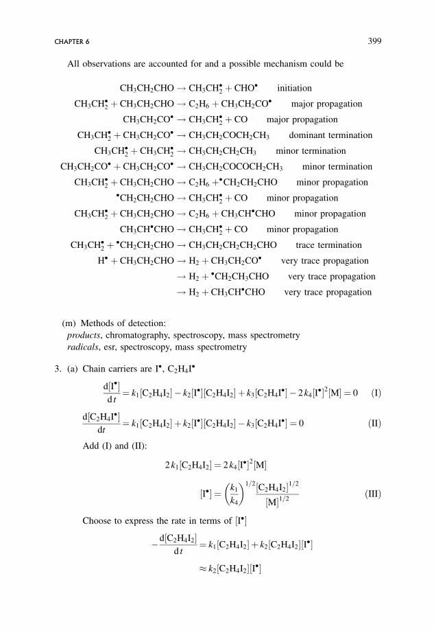
All observations are accounted for and a possible mechanism could be
CH3CH2CHO! CH3CH�2 þ CHO� initiation
CH3CH�2 þ CH3CH2CHO! C2H6 þ CH3CH2CO� major propagation
CH3CH2CO� ! CH3CH�2 þ CO major propagation
CH3CH�2 þ CH3CH2CO� ! CH3CH2COCH2CH3 dominant termination
CH3CH�2 þ CH3CH�2 ! CH3CH2CH2CH3 minor termination
CH3CH2CO� þ CH3CH2CO� ! CH3CH2COCOCH2CH3 minor termination
CH3CH�2 þ CH3CH2CHO! C2H6 þ�CH2CH2CHO minor propagation
�CH2CH2CHO! CH3CH�2 þ CO minor propagation
CH3CH�2 þ CH3CH2CHO! C2H6 þ CH3CH�CHO minor propagation
CH3CH�CHO! CH3CH�2 þ CO minor propagation
CH3CH�2 þ �CH2CH2CHO! CH3CH2CH2CH2CHO trace termination
H� þ CH3CH2CHO! H2 þ CH3CH2CO� very trace propagation
! H2 þ �CH2CH3CHO very trace propagation
! H2 þ CH3CH�CHO very trace propagation
(m) Methods of detection:
products, chromatography, spectroscopy, mass spectrometry
radicals, esr, spectroscopy, mass spectrometry
3. (a) Chain carriers are I�, C2H4I�
d½I��d t¼ k1½C2H4I2� � k2½I��½C2H4I2� þ k3½C2H4I�� � 2k4½I��2½M� ¼ 0 ðIÞ
d½C2H4I��dt
¼ k1½C2H4I2� þ k2½I��½C2H4I2� � k3½C2H4I�� ¼ 0 ðIIÞ
Add (I) and (II):
2k1½C2H4I2� ¼ 2k4½I��2½M�
½I�� ¼ k1
k4
� �1=2½C2H4I2�1=2
½M�1=2ðIIIÞ
Choose to express the rate in terms of ½I��
�d½C2H4I2�d t
¼ k1½C2H4I2� þ k2½C2H4I2�½I��
� k2½C2H4I2�½I��
CHAPTER 6 399
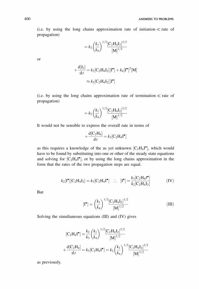
(i.e. by using the long chains approximation rate of initiation� rate of
propagation)
¼ k2
k1
k4
� �1=2½C2H4I2�3=2
½M�1=2
or
þd½I2�d t¼ k2½C2H4I2�½I�� þ k4½I��2½M�
� k2½C2H4I2�½I��
(i.e. by using the long chains approximation rate of termination� rate of
propagation)
¼ k2
k1
k4
� �1=2½C2H4I2�3=2
½M�1=2
It would not be sensible to express the overall rate in terms of
þd½C2H4�d t
¼ k3½C2H4I��
as this requires a knowledge of the as yet unknown ½C2H4I��, which would
have to be found by substituting into one or other of the steady state equations
and solving for ½C2H4I��, or by using the long chains approximation in the
form that the rates of the two propagation steps are equal.
k2½I��½C2H4I2� ¼ k3½C2H4I�� ; ½I�� ¼ k3½C2H4I��k2½C2H4I2�
ðIVÞ
But
½I�� ¼ k1
k4
� �1=2½C2H4I2�1=2
½M�1=2ðIIIÞ
Solving the simultaneous equations (III) and (IV) gives
½C2H4I�� ¼ k2
k3
k1
k4
� �1=2½C2H4I2�3=2
½M�1=2
þd½C2H4�d t
¼ k3½C2H4I�� ¼ k2
k1
k4
� �1=2½C2H4I2�3=2
½M�1=2
as previously.
400 ANSWERS TO PROBLEMS
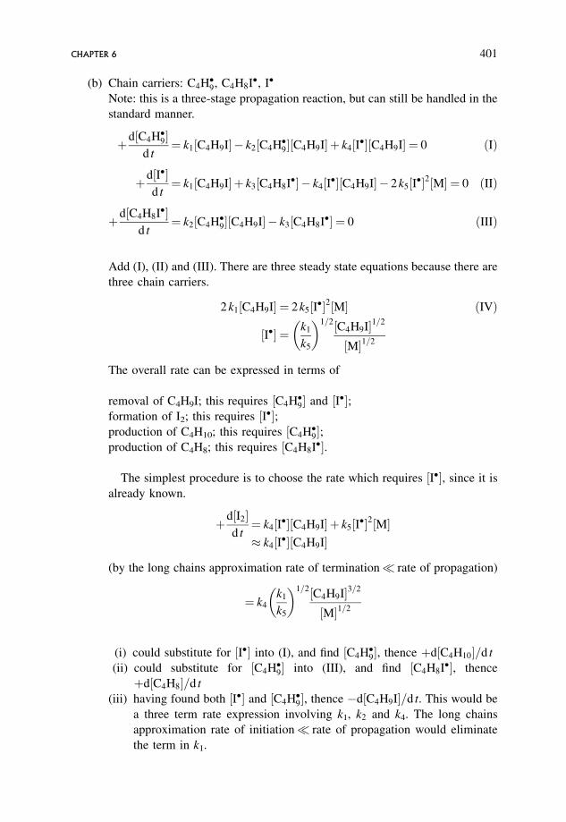
(b) Chain carriers: C4H�9, C4H8I�, I�
Note: this is a three-stage propagation reaction, but can still be handled in the
standard manner.
þd½C4H�9�d t
¼ k1½C4H9I� � k2½C4H�9�½C4H9I� þ k4½I��½C4H9I� ¼ 0 ðIÞ
þd½I��d t¼ k1½C4H9I� þ k3½C4H8I�� � k4½I��½C4H9I� � 2k5½I��2½M� ¼ 0 ðIIÞ
þd½C4H8I��d t
¼ k2½C4H�9�½C4H9I� � k3½C4H8I�� ¼ 0 ðIIIÞ
Add (I), (II) and (III). There are three steady state equations because there are
three chain carriers.
2 k1½C4H9I� ¼ 2k5½I��2½M� ðIVÞ
½I�� ¼ k1
k5
� �1=2½C4H9I�1=2
½M�1=2
The overall rate can be expressed in terms of
removal of C4H9I; this requires ½C4H�9� and ½I��;formation of I2; this requires ½I��;production of C4H10; this requires ½C4H�9�;production of C4H8; this requires ½C4H8I��.
The simplest procedure is to choose the rate which requires ½I��, since it is
already known.
þd½I2�d t¼ k4½I��½C4H9I� þ k5½I��2½M�� k4½I��½C4H9I�
(by the long chains approximation rate of termination� rate of propagation)
¼ k4
k1
k5
� �1=2½C4H9I�3=2
½M�1=2
(i) could substitute for ½I�� into (I), and find ½C4H�9�, thence þd½C4H10�=d t
(ii) could substitute for ½C4H�9� into (III), and find ½C4H8I��, thence
þd½C4H8�=d t
(iii) having found both ½I�� and ½C4H�9�, thence �d½C4H9I�=d t. This would be
a three term rate expression involving k1, k2 and k4. The long chains
approximation rate of initiation� rate of propagation would eliminate
the term in k1.
CHAPTER 6 401
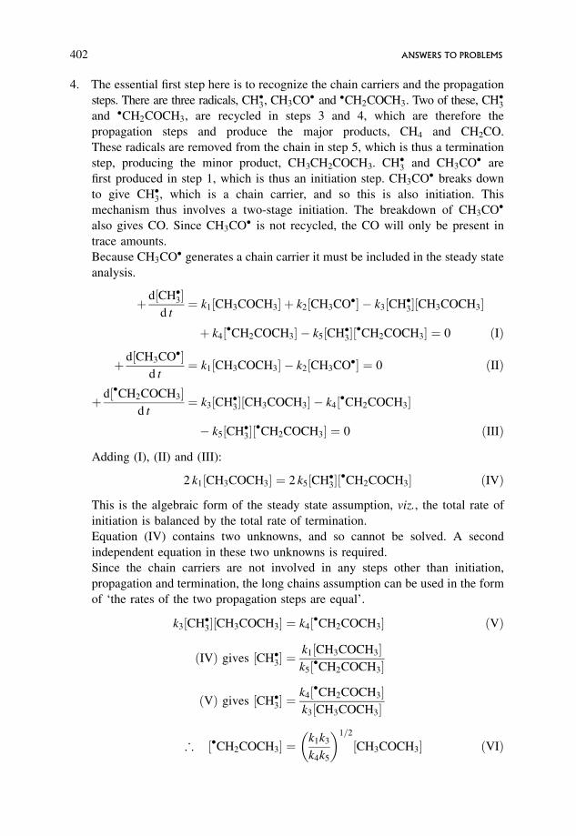
4. The essential first step here is to recognize the chain carriers and the propagation
steps. There are three radicals, CH�3, CH3CO� and �CH2COCH3. Two of these, CH�3and �CH2COCH3, are recycled in steps 3 and 4, which are therefore the
propagation steps and produce the major products, CH4 and CH2CO.
These radicals are removed from the chain in step 5, which is thus a termination
step, producing the minor product, CH3CH2COCH3. CH�3 and CH3CO� are
first produced in step 1, which is thus an initiation step. CH3CO� breaks down
to give CH�3, which is a chain carrier, and so this is also initiation. This
mechanism thus involves a two-stage initiation. The breakdown of CH3CO�
also gives CO. Since CH3CO� is not recycled, the CO will only be present in
trace amounts.
Because CH3CO� generates a chain carrier it must be included in the steady state
analysis.
þ d½CH�3�d t
¼ k1½CH3COCH3� þ k2½CH3CO�� � k3½CH�3�½CH3COCH3�
þ k4½�CH2COCH3� � k5½CH�3�½�CH2COCH3� ¼ 0 ðIÞ
þ d½CH3CO��d t
¼ k1½CH3COCH3� � k2½CH3CO�� ¼ 0 ðIIÞ
þ d½�CH2COCH3�d t
¼ k3½CH�3�½CH3COCH3� � k4½�CH2COCH3�
� k5½CH�3�½�CH2COCH3� ¼ 0 ðIIIÞ
Adding (I), (II) and (III):
2 k1½CH3COCH3� ¼ 2 k5½CH�3�½�CH2COCH3� ðIVÞ
This is the algebraic form of the steady state assumption, viz., the total rate of
initiation is balanced by the total rate of termination.
Equation (IV) contains two unknowns, and so cannot be solved. A second
independent equation in these two unknowns is required.
Since the chain carriers are not involved in any steps other than initiation,
propagation and termination, the long chains assumption can be used in the form
of ‘the rates of the two propagation steps are equal’.
k3½CH�3�½CH3COCH3� ¼ k4½�CH2COCH3� ðVÞ
ðIVÞ gives ½CH�3� ¼k1½CH3COCH3�k5½�CH2COCH3�
ðVÞ gives ½CH�3� ¼k4½�CH2COCH3�k3½CH3COCH3�
; ½�CH2COCH3� ¼k1k3
k4k5
� �1=2
½CH3COCH3� ðVIÞ
402 ANSWERS TO PROBLEMS
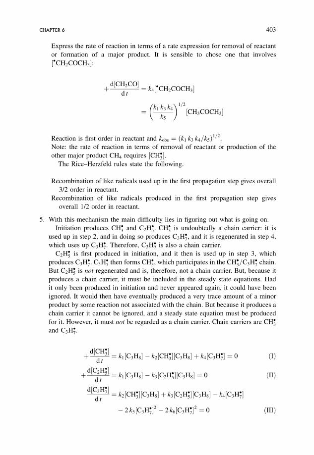
Express the rate of reaction in terms of a rate expression for removal of reactant
or formation of a major product. It is sensible to chose one that involves
½�CH2COCH3�:
þ d½CH2CO�d t
¼ k4½�CH2COCH3�
¼ k1 k3 k4
k5
� �1=2
½CH3COCH3�
Reaction is first order in reactant and kobs ¼ k1 k3 k4=k5ð Þ1=2.
Note: the rate of reaction in terms of removal of reactant or production of the
other major product CH4 requires ½CH�3�.The Rice–Herzfeld rules state the following.
Recombination of like radicals used up in the first propagation step gives overall
3/2 order in reactant.
Recombination of like radicals produced in the first propagation step gives
overall 1/2 order in reactant.
5. With this mechanism the main difficulty lies in figuring out what is going on.
Initiation produces CH�3 and C2H�5. CH�3 is undoubtedly a chain carrier: it is
used up in step 2, and in doing so produces C3H�7, and it is regenerated in step 4,
which uses up C3H�7. Therefore, C3H�7 is also a chain carrier.
C2H�5 is first produced in initiation, and it then is used up in step 3, which
produces C3H�7. C3H�7 then forms CH�3, which participates in the CH�3=C3H�7 chain.
But C2H�5 is not regenerated and is, therefore, not a chain carrier. But, because it
produces a chain carrier, it must be included in the steady state equations. Had
it only been produced in initiation and never appeared again, it could have been
ignored. It would then have eventually produced a very trace amount of a minor
product by some reaction not associated with the chain. But because it produces a
chain carrier it cannot be ignored, and a steady state equation must be produced
for it. However, it must not be regarded as a chain carrier. Chain carriers are CH�3and C3H�7.
þ d½CH�3�d t
¼ k1½C3H8� � k2½CH�3�½C3H8� þ k4½C3H�7� ¼ 0 ðIÞ
þ d½C2H�5�d t
¼ k1½C3H8� � k3½C2H�5�½C3H8� ¼ 0 ðIIÞ
d½C3H�7�d t
¼ k2½CH�3�½C3H8� þ k3½C2H�5�½C3H8� � k4½C3H�7�
� 2 k5½C3H�7�2 � 2 k6½C3H�7�
2 ¼ 0 ðIIIÞ
CHAPTER 6 403
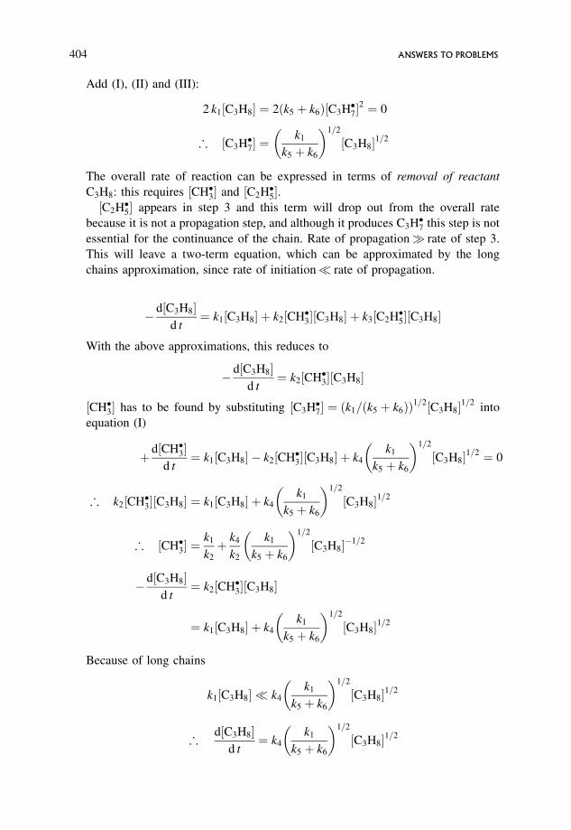
Add (I), (II) and (III):
2 k1½C3H8� ¼ 2ðk5 þ k6Þ½C3H�7�2 ¼ 0
; ½C3H�7� ¼k1
k5 þ k6
� �1=2
½C3H8�1=2
The overall rate of reaction can be expressed in terms of removal of reactant
C3H8: this requires ½CH�3� and ½C2H�5�.½C2H�5� appears in step 3 and this term will drop out from the overall rate
because it is not a propagation step, and although it produces C3H�7 this step is not
essential for the continuance of the chain. Rate of propagation� rate of step 3.
This will leave a two-term equation, which can be approximated by the long
chains approximation, since rate of initiation� rate of propagation.
� d½C3H8�d t
¼ k1½C3H8� þ k2½CH�3�½C3H8� þ k3½C2H�5�½C3H8�
With the above approximations, this reduces to
� d½C3H8�d t
¼ k2½CH�3�½C3H8�
½CH�3� has to be found by substituting ½C3H�7� ¼ k1=ðk5 þ k6Þð Þ1=2½C3H8�1=2into
equation (I)
þ d½CH�3�d t
¼ k1½C3H8� � k2½CH�3�½C3H8� þ k4
k1
k5 þ k6
� �1=2
½C3H8�1=2 ¼ 0
; k2½CH�3�½C3H8� ¼ k1½C3H8� þ k4
k1
k5 þ k6
� �1=2
½C3H8�1=2
; ½CH�3� ¼k1
k2
þ k4
k2
k1
k5 þ k6
� �1=2
½C3H8��1=2
� d½C3H8�d t
¼ k2½CH�3�½C3H8�
¼ k1½C3H8� þ k4
k1
k5 þ k6
� �1=2
½C3H8�1=2
Because of long chains
k1½C3H8� � k4
k1
k5 þ k6
� �1=2
½C3H8�1=2
;d½C3H8�
d t¼ k4
k1
k5 þ k6
� �1=2
½C3H8�1=2
404 ANSWERS TO PROBLEMS
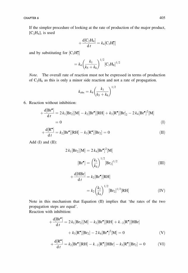
If the simpler procedure of looking at the rate of production of the major product,
[C2H4], is used
þ d½C2H4�d t
¼ k4½C3H�7�
and by substituting for ½C3H�7�
¼ k4
k1
k5 þ k6
� �1=2
½C3H8�1=2
Note. The overall rate of reaction must not be expressed in terms of production
of C2H6 as this is only a minor side reaction and not a rate of propagation.
kobs ¼ k4
k1
k5 þ k6
� �1=2
6. Reaction without inhibition:
þ d½Br��d t¼ 2 k1½Br2�½M� � k2½Br��½RH� þ k3½R��½Br�2 � 2 k4½Br��2½M�
¼ 0 ðIÞ
þ d½R��d t¼ k2½Br��½RH� � k3½R��½Br2� ¼ 0 ðIIÞ
Add (I) and (II):
2 k1½Br2�½M� ¼ 2 k4½Br��2½M�
½Br�� ¼ k1
k4
� �1=2
½Br2�1=2 ðIIIÞ
þ d½HBr�d t
¼ k2½Br��½RH�
¼ k2
k1
k4
� �1=2
½Br2�1=2½RH� ðIVÞ
Note in this mechanism that Equation (II) implies that ‘the rates of the two
propagation steps are equal’.
Reaction with inhibition:
þ d½Br��d t¼ 2 k1½Br2�½M� � k2½Br��½RH� þ k�2½R��½HBr�
þ k3½R��½Br2� � 2 k4½Br��2½M� ¼ 0 ðVÞ
þ d½R��d t¼ k2½Br��½RH� � k�2½R��½HBr� � k3½R��½Br2� ¼ 0 ðVIÞ
CHAPTER 6 405
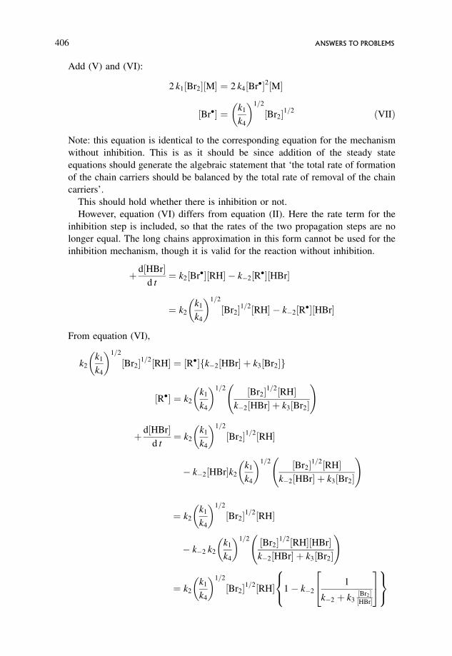
Add (V) and (VI):
2 k1½Br2�½M� ¼ 2 k4½Br��2½M�
½Br�� ¼ k1
k4
� �1=2
½Br2�1=2 ðVIIÞ
Note: this equation is identical to the corresponding equation for the mechanism
without inhibition. This is as it should be since addition of the steady state
equations should generate the algebraic statement that ‘the total rate of formation
of the chain carriers should be balanced by the total rate of removal of the chain
carriers’.
This should hold whether there is inhibition or not.
However, equation (VI) differs from equation (II). Here the rate term for the
inhibition step is included, so that the rates of the two propagation steps are no
longer equal. The long chains approximation in this form cannot be used for the
inhibition mechanism, though it is valid for the reaction without inhibition.
þ d½HBr�d t
¼ k2½Br��½RH� � k�2½R��½HBr�
¼ k2
k1
k4
� �1=2
½Br2�1=2½RH� � k�2½R��½HBr�
From equation (VI),
k2
k1
k4
� �1=2
½Br2�1=2½RH� ¼ ½R��fk�2½HBr� þ k3½Br2�g
½R�� ¼ k2
k1
k4
� �1=2 ½Br2�1=2½RH�k�2½HBr� þ k3½Br2�
!
þ d½HBr�d t
¼ k2
k1
k4
� �1=2
½Br2�1=2½RH�
� k�2½HBr�k2
k1
k4
� �1=2 ½Br2�1=2½RH�k�2½HBr� þ k3½Br2�
!
¼ k2
k1
k4
� �1=2
½Br2�1=2½RH�
� k�2 k2
k1
k4
� �1=2 ½Br2�1=2½RH�½HBr�k�2½HBr� þ k3½Br2�
!
¼ k2
k1
k4
� �1=2
½Br2�1=2½RH� 1� k�2
1
k�2 þ k3½Br2�½HBr�
24
35
8<:
9=;
406 ANSWERS TO PROBLEMS
Note: the presence of the inhibition step dramatically complicates the rate
expression.
7. Step 1 is the unimolecular decomposition of a diatomic molecule, and step �1 is a
recombination of two atoms. This recombination is a highly exothermic reaction,
and this energy will reside in the newly formed bond, which is thus highly excited.
If this energy is not removed in the time of one vibration, the molecule will split
up on vibration and recombination will not occur. If a collision occurs before the
first vibration, then energy transfer takes place and the bond will be stabilized. The
third body fulfils this function. This is more effective at high pressures and low
temperatures.
The decomposition of the diatomic molecule is the reverse of the recom-
bination step, and so will also require a third body. The physical process
involved is transfer of energy by collision to form an activated molecule which
has enough energy to react. This is more efficient at high pressures and low
temperatures.
Steps 4 and 5 are recombinations of large radicals. Here there are sufficient
normal modes of vibration for the newly formed bond to be stabilized by transfer
of the excess energy around the molecule via the normal modes of vibration. The
product in step 4 has 36 normal modes, while the product in step 5 has 18. It is
only at very low pressures and very high temperatures that 18 normal modes
would be insufficient to stabilize the C��C bond that is formed.
OH� þ H� ! H2O
The product has three normal modes only, and a third body is necessary under all
normal conditions.
CH�3 þ CH�3 ! C2H6
The product has 18 normal modes, and for ordinary pressures and temperatures
these will be sufficient to stabilize the C��C bond. This may not be the case at very
low pressures and very high temperatures; compare with Cl� þ C2H4Cl�.
H� þ I� ! HI
The product is a diatomic molecule, and a third body is necessary under all
conditions; compare with Cl� þ Cl�
CH�3 þ ðCH3Þ3C� ! ðCH3Þ3CCH3
The product has 45 normal modes of vibration, and under all conditions a third
body will not be required. It is unlikely that there is a range of pressures and
temperatures for which this number of normal modes would be insufficient for
efficient energy transfer around the molecule.
8. This is a photochemical reaction, hence the initiation step is likely to be splitting
of Cl2 into two Cl� atoms.
Cl2 þ h � ! 2 Cl�
CHAPTER 6 407
There is no need for a third body to supply activation energy since this is achieved
by the radiation. It is also a chain reaction as is shown by the quantum yield of
>100. Only one product is observed, and this must be formed in propagation. It
has two Cl added and these must be added one at a time to fit a propagation step.
This suggests that a Cl� must add in the first propagation step. There are no H
atoms in the reactant so this first propagation step cannot be a H abstraction
reaction. Since only one product is formed there can be no major product formed
in the first propagation step. All of this suggests
Cl� þ C6F10 ! C6F10Cl�
as the first propagation step.
The second propagation step must add a further Cl, regenerate Cl� and form the
product:
Cl2 þ C6F10Cl� ! C6F10Cl2 þ Cl�
The termination step must produce no other product, and possible typical steps
are radical/radical or atom/atom recombinations.
� Cl� þ Cl� ! Cl2, possible since Cl2 is a reactant and would not be detected as
a minor product.
� C6F10Cl� þ Cl� ! C6F10Cl2. This is the major product produced in propaga-
tion, and would not be detected as a minor product.
It is now necessary to see whether either of these possible mechanisms fit the
observed kinetics. This requires a steady state treatment on both mechanisms
to find the predicted rate expressions to compare with the observed expression.
The observed kinetics are
� d½C6F10�d t
¼ kobsI1=2abs ½Cl2�
� Mechanism 1.
Cl2 þ h � ! 2 Cl�
Cl� þ C6F10!k2
C6F10Cl�
Cl2 þ C6F10Cl� !k3C6F10Cl2 þ Cl�
Cl� þ Cl� þM!k4Cl2 þM
� Mechanism 2.
Cl2 þ h � ! 2 Cl�
Cl� þ C6F10!k2
C6F10Cl�
Cl2 þ C6F10Cl� !k3C6F10Cl2 þ Cl�
C6F10Cl� þ Cl� !k5C6F10Cl2
408 ANSWERS TO PROBLEMS
� Steady state treatment on mechanism 1.
d½Cl��d t¼ 2 Iabs � k2½Cl��½C6F10� þ k3½C6F10Cl��½Cl2� � 2 k4½Cl��2½M� ¼ 0
d½C6F10Cl��d t
¼ k2½Cl��½C6F10� � k3½C6F10Cl��½Cl2� ¼ 0
Adding the steady state equations gives
2 Iabs ¼ 2 k4½Cl��2½M�
; ½Cl�� ¼ Iabs
k4
� �1=2
½M��1=2
� d½C6F10�d t
¼ k2½Cl��½C6F10� ¼ k2
Iabs
k4
� �1=2
½M��1=2½C6F10�
This does not fit the observed kinetics, and so mechanism 1 is not correct.
� Steady state treatment on mechanism 2.
d½Cl��d t¼ 2 Iabs � k2½Cl��½C6F10� þ k3½C6F10Cl��½Cl2�
� k5½Cl��½C6F10Cl�� ¼ 0
d½C6F10Cl��d t
¼ k2½Cl��½C6F10� � k3½C6F10Cl��½Cl2� � k5½Cl��½C6F10Cl�� ¼ 0
Adding the steady state equations gives
2 Iabs ¼ 2 k5½Cl��½C6F10Cl��
; ½Cl�� ¼ Iabs
k5½C6F10Cl��
Assuming long chains, the rates of the two propagation steps are equal:
k2½Cl��½C6F10� ¼ k3½C6F10Cl��½Cl2�
½Cl�� ¼ k3½C6F10Cl��½Cl2�k2½C6F10�
Taking the two expressions for ½Cl�� gives
½C6F10Cl�� ¼ k2Iabs
k3 k5
� �1=2 ½C6F10�½Cl2�
� �1=2
Expressing the rate in a form which involves this radical concentration,
� d½Cl2�d t¼ Iabs þ k3½C6F10Cl��½Cl2� � k3½C6F10Cl��½Cl2�
¼ k2k3Iabs
k5
� �1=2
½C6F10�1=2½Cl2�1=2
CHAPTER 6 409
The term in I drops out because of the long chains approximation.
This expression does not fit the observed kinetics, and mechanism 2 is not
correct.
Neither of the two possible termination steps fit the observed kinetics. The third
possibility would give a product that was not detected:
C6F10Cl� þ C6F10Cl� ! C12F20Cl2
However, although recombination steps are very common termination steps, dis-
proportionation reactions are also found.
C6F10Cl� þ C6F10Cl� !k6C6F10 þ C6F10Cl2
This would give as minor products the reactant and the major product with the
following mechanism.
� Mechanism 3.
Cl2 þ h � ! 2 Cl�
Cl� þ C6F10!k2
C6F10Cl�
Cl2 þ C6F10Cl� !k3C6F10Cl2 þ Cl�
C6F10Cl� þ C6F10Cl� !k6C6F10Cl2 þ C6F10
� Steady state treatment on mechanism 3.
d½Cl��d t¼ 2 Iabs � k2½Cl��½C6F10� þ k3½C6F10Cl��½Cl2� ¼ 0
d½C6F10Cl��d t
¼ k2½Cl��½C6F10� � k3½C6F10Cl��½Cl2� � 2 k6½C6F10Cl��2 ¼ 0
Adding the steady state equations gives
2 Iabs ¼ 2 k6½C6F10Cl��2
; ½C6F10Cl�� ¼ Iabs
k6
� �1=2
� d½Cl2�d t¼ Iabs þ k3½C6F10Cl��½Cl2� � k3½C6F10Cl��½Cl2�
¼ k3
Iabs
k6
� �1=2
½Cl2�
410 ANSWERS TO PROBLEMS
Long chains allows the term in Iabs to drop out.
This expression fits the observed kinetics, and so mechanism 3 involving
a disproportionation termination step is a possible mechanism for this reaction.
Chapter 7
1. For the reaction
Aþ Bþ C! activated complex
k ¼ k0
A B C
6¼
log10 k ¼ log10 k0 þ log10 A þ log10 B þ log10 C � log10 6¼
where log10 i ¼ �A z2i
ffiffiIp
For the reaction quoted two mechanisms can be written:
� HEþ þ H3Oþ !
HEþ þ H3Oþ þ SO2�4 !
and
� HEþ þ H3Oþ !
HEþ þ HSO�4 !
For the first mechanism HEþ þ H3Oþ þ SO2�4 ! an activated complex which is
overall neutral.
log10 kSO2�4¼ log10 k0 þ log10 HEþ þ log10 H3Oþ þ log10 SO2�
4� log10 6¼
¼ log10 k0 � A 12 ffiffiIp� A 12
ffiffiIp� A 22
ffiffiIp
þ A 02 ffiffiIp
¼ log10 k0 � 6 AffiffiIp
For the second mechanism HEþ þ HSO�4 ! an activated complex which is
overall neutral.
log10 kHSO�4¼ log10 k0 þ log10 HEþ þ log10 HSO�4
� log10 6¼
¼ log10 k0 � A 12 ffiffiIp� A 12
ffiffiIpþ A 02
ffiffiIp
¼ log10 k0 � 2 AffiffiIp
CHAPTER 7 411
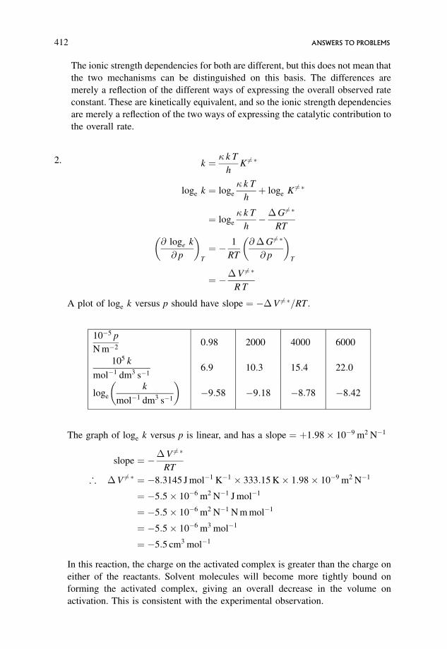
The ionic strength dependencies for both are different, but this does not mean that
the two mechanisms can be distinguished on this basis. The differences are
merely a reflection of the different ways of expressing the overall observed rate
constant. These are kinetically equivalent, and so the ionic strength dependencies
are merely a reflection of the two ways of expressing the catalytic contribution to
the overall rate.
2. k ¼ � k T
hK 6¼ �
loge k ¼ loge
� k T
hþ loge K 6¼ �
¼ loge
� k T
h��G 6¼ �
RT
@ loge k
@ p
� �T
¼ � 1
RT
@�G6¼ �
@ p
� �T
¼ ��V 6¼ �
R T
A plot of loge k versus p should have slope ¼ ��V 6¼ �=RT .
10�5 p
N m�20:98 2000 4000 6000
105 k
mol�1 dm3 s�16:9 10:3 15:4 22:0
loge
k
mol�1 dm3 s�1
� ��9:58 �9:18 �8:78 �8:42
The graph of loge k versus p is linear, and has a slope ¼ þ1:98 10�9 m2 N�1
slope ¼ ��V 6¼ �
RT
; �V 6¼ � ¼ �8:3145 J mol�1 K�1 333:15 K 1:98 10�9 m2 N�1
¼ �5:5 10�6 m2 N�1 J mol�1
¼ �5:5 10�6 m2 N�1 N m mol�1
¼ �5:5 10�6 m3 mol�1
¼ �5:5 cm3 mol�1
In this reaction, the charge on the activated complex is greater than the charge on
either of the reactants. Solvent molecules will become more tightly bound on
forming the activated complex, giving an overall decrease in the volume on
activation. This is consistent with the experimental observation.
412 ANSWERS TO PROBLEMS
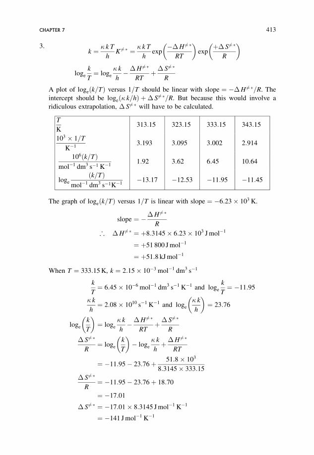
3.k ¼ � k T
hK 6¼ � ¼ � k T
hexp
��H 6¼ �
RT
� �exp
þ� S6¼ �
R
� �
loge
k
T¼ loge
� k
h��H 6¼ �
RTþ� S6¼ �
R
A plot of logeðk=TÞ versus 1=T should be linear with slope ¼ ��H 6¼ �=R. The
intercept should be logeð� k=hÞ þ� S6¼ �=R. But because this would involve a
ridiculous extrapolation, � S6¼ � will have to be calculated.
T
K313:15 323:15 333:15 343:15
103 1=T
K�13:193 3:095 3:002 2:914
106ðk=TÞmol�1 dm3 s�1 K�1
1:92 3:62 6:45 10:64
loge
ðk=TÞmol�1 dm3 s�1K�1
�13:17 �12:53 �11:95 �11:45
The graph of logeðk=TÞ versus 1=T is linear with slope ¼ �6:23 103 K.
slope ¼ ��H 6¼ �
R
; �H 6¼ � ¼ þ8:3145 6:23 103 J mol�1
¼ þ51 800 J mol�1
¼ þ51:8 kJ mol�1
When T ¼ 333:15 K, k ¼ 2:15 10�3 mol�1 dm3 s�1
k
T¼ 6:45 10�6 mol�1 dm3 s�1 K�1 and loge
k
T¼ �11:95
� k
h¼ 2:08 1010 s�1 K�1 and loge
� k
h
� �¼ 23:76
loge
k
T
� �¼ loge
� k
h��H 6¼ �
RTþ� S6¼ �
R
� S6¼ �
R¼ loge
k
T
� �� loge
� k
hþ�H 6¼ �
RT
¼ �11:95� 23:76þ 51:8 103
8:3145 333:15
� S6¼ �
R¼ �11:95� 23:76þ 18:70
¼ �17:01
� S6¼ � ¼ �17:01 8:3145 J mol�1 K�1
¼ �141 J mol�1 K�1
CHAPTER 7 413
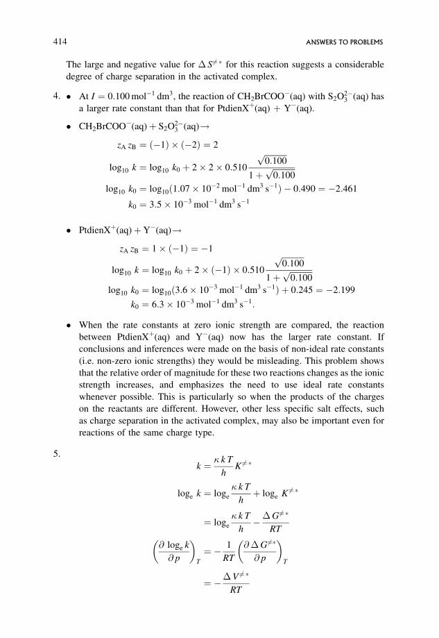
The large and negative value for � S6¼ � for this reaction suggests a considerable
degree of charge separation in the activated complex.
4. � At I ¼ 0:100 mol�1 dm3, the reaction of CH2BrCOO�(aq) with S2O2�3 (aq) has
a larger rate constant than that for PtdienXþ(aq) þ Y�(aq).
� CH2BrCOO�(aq)þ S2O2�3 (aq)!
zA zB ¼ ð�1Þ ð�2Þ ¼ 2
log10 k ¼ log10 k0 þ 2 2 0:510
ffiffiffiffiffiffiffiffiffiffiffi0:100p
1þffiffiffiffiffiffiffiffiffiffiffi0:100p
log10 k0 ¼ log10ð1:07 10�2 mol�1 dm3 s�1Þ � 0:490 ¼ �2:461
k0 ¼ 3:5 10�3 mol�1 dm3 s�1
� PtdienXþ(aq)þY�(aq)!
zA zB ¼ 1 ð�1Þ ¼ �1
log10 k ¼ log10 k0 þ 2 ð�1Þ 0:510
ffiffiffiffiffiffiffiffiffiffiffi0:100p
1þffiffiffiffiffiffiffiffiffiffiffi0:100p
log10 k0 ¼ log10ð3:6 10�3 mol�1 dm3 s�1Þ þ 0:245 ¼ �2:199
k0 ¼ 6:3 10�3 mol�1 dm3 s�1:
� When the rate constants at zero ionic strength are compared, the reaction
between PtdienXþ(aq) and Y�(aq) now has the larger rate constant. If
conclusions and inferences were made on the basis of non-ideal rate constants
(i.e. non-zero ionic strengths) they would be misleading. This problem shows
that the relative order of magnitude for these two reactions changes as the ionic
strength increases, and emphasizes the need to use ideal rate constants
whenever possible. This is particularly so when the products of the charges
on the reactants are different. However, other less specific salt effects, such
as charge separation in the activated complex, may also be important even for
reactions of the same charge type.
5.
k ¼ � k T
hK 6¼ �
loge k ¼ loge
� k T
hþ loge K 6¼ �
¼ loge
� k T
h��G 6¼ �
RT
@ loge k
@ p
� �T
¼ � 1
RT
@�G6¼�
@ p
� �T
¼ ��V 6¼ �
RT
414 ANSWERS TO PROBLEMS
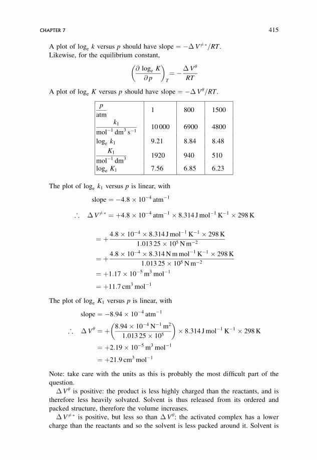
A plot of loge k versus p should have slope ¼ ��V 6¼ �=RT .
Likewise, for the equilibrium constant,
@ loge K
@ p
� �T
¼ ��V�
RT
A plot of loge K versus p should have slope ¼ ��V�=RT .
p
atm1 800 1500
k1
mol�1 dm3 s�110 000 6900 4800
loge k1 9:21 8:84 8:48
K1
mol�1 dm31920 940 510
loge K1 7:56 6:85 6:23
The plot of loge k1 versus p is linear, with
slope ¼ �4:8 10�4 atm�1
; �V 6¼ � ¼ þ4:8 10�4 atm�1 8:314 J mol�1 K�1 298 K
¼ þ 4:8 10�4 8:314 J mol�1 K�1 298 K
1:013 25 105 N m�2
¼ þ 4:8 10�4 8:314 N m mol�1 K�1 298 K
1:013 25 105 N m�2
¼ þ1:17 10�5 m3 mol�1
¼ þ11:7 cm3 mol�1
The plot of loge K1 versus p is linear, with
slope ¼ �8:94 10�4 atm�1
; �V� ¼ þ 8:94 10�4 N�1 m2
1:013 25 105
� � 8:314 J mol�1 K�1 298 K
¼ þ2:19 10�5 m3 mol�1
¼ þ21:9 cm3 mol�1
Note: take care with the units as this is probably the most difficult part of the
question.
�V� is positive: the product is less highly charged than the reactants, and is
therefore less heavily solvated. Solvent is thus released from its ordered and
packed structure, therefore the volume increases.
�V 6¼ � is positive, but less so than �V�: the activated complex has a lower
charge than the reactants and so the solvent is less packed around it. Solvent is
CHAPTER 7 415
thus released from the solvation sheaths, and therefore the volume increases on
forming the activated complex.
The magnitude of �V 6¼ � is less than that for �V�, indicating that the solvation
arrangement and charge neutralization is not so fully developed on forming the
activated complex as when the final product is formed. The activated complex
does resemble the products somewhat, and is probably half-way between reactants
and products.
Note how solvation is dominant here: two species! one activated complex!one product. On this basis a decrease in volume for both processes would be
expected. This is not observed.
6. For reactions 1–3, �V 6¼ � and �V� are very similar with �V 6¼ � only slightly less
negative than �V�. This suggests that the activated complex is very similar to the
products, but not quite as compact.
For reactions 4 and 5, �V 6¼ � is more negative than �V�, which suggests an
activated complex which resembles the product, but is even more compact than the
product. Such possibilities complicate possible interpretations of values of �V 6¼ �.For the reverse reactions
�V6¼ �b values are þ6.1, þ6.8, þ4.3, �5.0 and �1:5 cm3 mol�1, and
�V�b values are þ36.9, þ37.0, þ37.2þ 36.3 and þ 35:5 cm3 mol�1.
None of the �V6¼ �b values is very large and all are very different from the
corresponding �V�b values. The reverse reactions are 1! 2, and so the �V
6¼ �b
values would be expected to be positive and fairly large. This is not the case,
which suggests that the activated complexes are fairly similar to the reactant C.
A similar trend in � S6¼ � values for both forward and back reactions would be
expected, though the � S6¼ � values are complicated by the fact that the complexity
of the reactants must be considered.
Chapter 8
1. Mechanistic rate ¼ k1½A�½NH3� þ k2½A�
Note: there is no [H2O] in the last term since H2O is the solvent, and is thus in
excess.
Observed rate ¼ kobs½A�where kobs is a pseudo-first order rate constant, see units in table to confirm.
; kobs ¼ k1½NH3� þ k2
; kobs versus [NH3] should be linear, with slope ¼ k1 and intercept ¼ k2.
416 ANSWERS TO PROBLEMS
The graph is linear, confirming the analysis, and gives
k1 ¼ slope ¼ 3:55 10�4 mol�1 dm3 s�1, and k2 ¼ intercept ¼ 4:2 10�5 s�1.
2. Mechanistic rate ¼ k2½E�actual ½OH��actual þ k3½HEþ�actual½OH��actual
þ k4½E�actual½OH��actual½M2þ�actual
The most sensible way in which to follow this reaction would be at constant pH,
and so the observed rate can be expressed as
observed rate ¼ kobs½E�total½OH��actual
with kobs being a second order rate constant as required.
kobs½E�total½OH��actual ¼ k2½E�actual½OH��actual þ k3½HEþ�actual½OH��actual
þ k4½E�actual½OH��actual½M2þ�actual
kobs ¼ k2
½E�actual
½E�total
þ k3
½HEþ�actual
½E�total
þ k4½M2þ� ½E�actual
½E�total
½E�total ¼ ½E�actual þ ½HEþ�actual
Eþ H2O �! �k1
k�1
HEþ þ OH�
K1 ¼½HEþ�½OH��½E�
� �equil
½HEþ�actual ¼K1½E�actual
½OH��actual
; kobs ¼ k2
½E�actual
½E�total
þ k3 K1
½E�actual
½E�total½OH��actual
þ k4½M2þ� ½E�actual
½E�total
p K1 ¼ 6:3, and K1 ¼ 5:0 10�7 mol dm�3, hence no extensive protonation will
occur, and so
½E�total � ½E�actual and ½HEþ�actual ¼K1½E�actual
½OH��actual
� K1½E�total
½OH��actual
; kobs ¼ k2
½E�total
½E�total
þ k3 K1
½E�total
½E�total½OH��actual
þ k4½M2þ� ½E�total
½E�total
; kobs ¼ k2 þ k3
K1
½OH��actual
þ k4½M2þ�actual
k2 and k3 can be found from values of kobs found at various pH values, i.e. [OH�]
in the absence of added M2þ.
; kobs ¼ k2 þ k3
K1
½OH��actual
CHAPTER 8 417
A plot of kobs versus 1=½OH��actual should be linear with intercept ¼ k2 and
slope ¼ k3 K1. Since K1 is known, then k3 can be found.
k4 can then be found by following the hydrolysis at one pH, i.e. at one value of
[OH�], but in the presence of varying [M2þ].
; kobs � k2 þ k3
K1
½OH��actual
� �¼ k4½M2þ�actual
All quantities on the left hand side of this equation can either be measured or
calculated. A graph of kobs � k2 � k3 K1=½OH�actual versus ½M2þ�actual should be
linear, going through the origin and with slope k4.
3. A solution containing Tlþ(aq) will also contain the ion pair TlOH(aq).
TlþðaqÞ þ OH�ðaqÞ�! �TlOHðaqÞ
K ¼ ½TlOH�½Tlþ�½OH��
� �equil
If there is a dependence of the rate of hydrolysis on ½Tlþ�, it is likely that the ion
pair also reacts with the ester.
Eþ OH� �!k products
Eþ TlOH��!kTlOHproducts
Mechanistic rate:
� d½E�total
d t¼ k½E�½OH��actual þ kTlOH½E�½TlOH�actual
Observed rate:
� d½E�total
d t¼ kobs½E�½OH��actual
; kobs½E�½OH��actual ¼ k½E�½OH��actual þ kTlOH½E�½TlOH�actual
; kobs ¼ k þ kTlOH
½TlOH�actual
½OH��actual
� �¼ k þ kTlOH K½Tlþ�actual
K ¼ 6 mol�1 dm3. This value for the association constant indicates that the
fraction of Tlþ associated is low when [OH�] is sufficiently low, and so the
relation
½Tlþ�total ¼ ½Tlþ�actual þ ½TlOH�actual
418 ANSWERS TO PROBLEMS
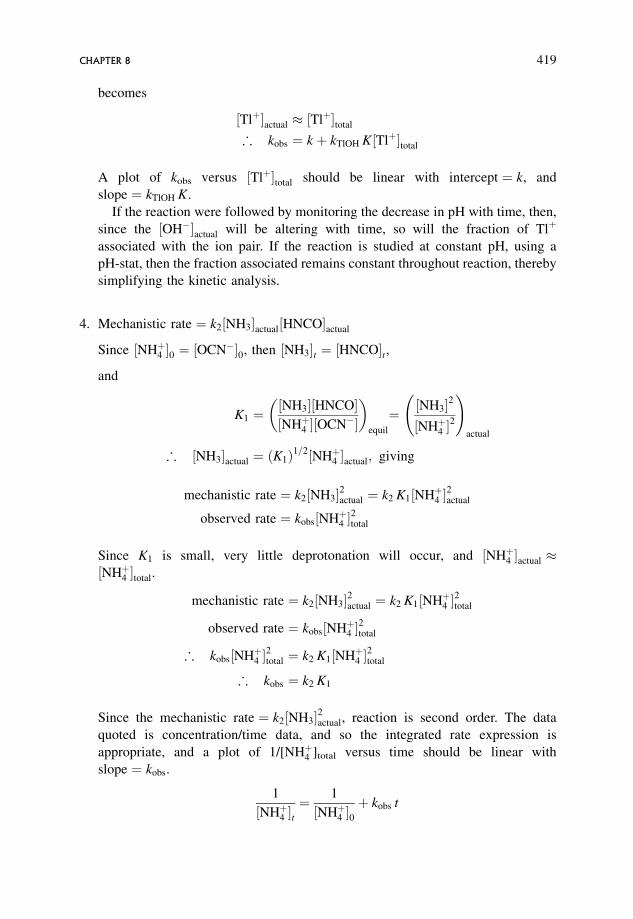
becomes
½Tlþ�actual � ½Tlþ�total
; kobs ¼ k þ kTlOH K½Tlþ�total
A plot of kobs versus ½Tlþ�total should be linear with intercept ¼ k, and
slope ¼ kTlOH K.
If the reaction were followed by monitoring the decrease in pH with time, then,
since the ½OH��actual will be altering with time, so will the fraction of Tlþ
associated with the ion pair. If the reaction is studied at constant pH, using a
pH-stat, then the fraction associated remains constant throughout reaction, thereby
simplifying the kinetic analysis.
4. Mechanistic rate ¼ k2½NH3�actual½HNCO�actual
Since ½NHþ4 �0 ¼ ½OCN��0, then ½NH3�t ¼ ½HNCO�t,
and
K1 ¼½NH3�½HNCO�½NHþ4 �½OCN��
� �equil
¼ ½NH3�2
½NHþ4 �2
!actual
; ½NH3�actual ¼ ðK1Þ1=2½NHþ4 �actual; giving
mechanistic rate ¼ k2½NH3�2actual ¼ k2 K1½NHþ4 �2actual
observed rate ¼ kobs½NHþ4 �2total
Since K1 is small, very little deprotonation will occur, and ½NHþ4 �actual �½NHþ4 �total.
mechanistic rate ¼ k2½NH3�2actual ¼ k2 K1½NHþ4 �2total
observed rate ¼ kobs½NHþ4 �2total
; kobs½NHþ4 �2total ¼ k2 K1½NHþ4 �
2total
; kobs ¼ k2 K1
Since the mechanistic rate ¼ k2½NH3�2actual, reaction is second order. The data
quoted is concentration/time data, and so the integrated rate expression is
appropriate, and a plot of 1/[NHþ4 ]total versus time should be linear with
slope ¼ kobs.
1
½NHþ4 �t¼ 1
½NHþ4 �0þ kobs t
CHAPTER 8 419
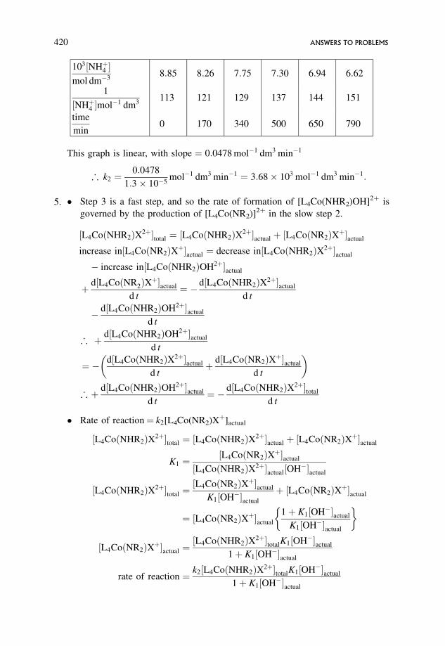
103½NHþ4 �mol dm�3
8:85 8:26 7:75 7:30 6:94 6:62
1
½NHþ4 �mol�1 dm3113 121 129 137 144 151
time
min0 170 340 500 650 790
This graph is linear, with slope ¼ 0:0478 mol�1 dm3 min�1
; k2 ¼0:0478
1:3 10�5mol�1 dm3 min�1 ¼ 3:68 103 mol�1 dm3 min�1:
5. � Step 3 is a fast step, and so the rate of formation of [L4Co(NHR2)OH]2þ is
governed by the production of [L4Co(NR2)]2þ in the slow step 2.
½L4CoðNHR2ÞX2þ�total ¼ ½L4CoðNHR2ÞX2þ�actual þ ½L4CoðNR2ÞXþ�actual
increase in½L4CoðNR2ÞXþ�actual ¼ decrease in½L4CoðNHR2ÞX2þ�actual
� increase in½L4CoðNHR2ÞOH2þ�actual
þ d½L4CoðNR2ÞXþ�actual
d t¼ � d½L4CoðNHR2ÞX2þ�actual
d t
� d½L4CoðNHR2ÞOH2þ�actual
d t
; þ d½L4CoðNHR2ÞOH2þ�actual
d t
¼ � d½L4CoðNHR2ÞX2þ�actual
d tþ d½L4CoðNR2ÞXþ�actual
d t
� �
;þ d½L4CoðNHR2ÞOH2þ�actual
d t¼ � d½L4CoðNHR2ÞX2þ�total
d t
� Rate of reaction¼ k2[L4Co(NR2)Xþ]actual
½L4CoðNHR2ÞX2þ�total ¼ ½L4CoðNHR2ÞX2þ�actual þ ½L4CoðNR2ÞXþ�actual
K1 ¼½L4CoðNR2ÞXþ�actual
½L4CoðNHR2ÞX2þ�actual½OH��actual
½L4CoðNHR2ÞX2þ�total ¼½L4CoðNR2ÞXþ�actual
K1½OH��actual
þ ½L4CoðNR2ÞXþ�actual
¼ ½L4CoðNR2ÞXþ�actual
1þ K1½OH��actual
K1½OH��actual
� �
½L4CoðNR2ÞXþ�actual ¼½L4CoðNHR2ÞX2þ�totalK1½OH��actual
1þ K1½OH��actual
rate of reaction ¼ k2½L4CoðNHR2ÞX2þ�totalK1½OH��actual
1þ K1½OH��actual
420 ANSWERS TO PROBLEMS
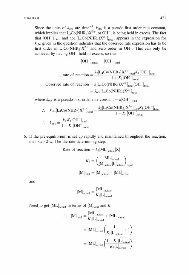
Since the units of kobs are time�1, kobs is a pseudo-first order rate constant,
which implies that L4Co(NHR2)X2þ, or OH�, is being held in excess. The fact
that [OH�]total, and not ½L4CoðNHR2ÞX2þ�total, appears in the expression for
kobs given in the question indicates that the observed rate expression has to be
first order in L4Co(NHR2)X2þ and zero order in OH�. This can only be
achieved by having OH� held in excess, so that
½OH��actual ¼ ½OH��total
; rate of reaction ¼ k2½L4CoðNHR2ÞX2þ�totalK1½OH��total
1þ K1½OH��total
Observed rate of reaction ¼ k½L4CoðNHR2ÞX2þ�total½OH��total
¼ kobs½L4CoðNHR2ÞX2þ�total
where kobs is a pseudo-first order rate constant ¼ k½OH��total
; kobs½L4CoðNHR2ÞX2þ�total ¼k2½L4CoðNHR2ÞX2þ�totalK1½OH��total
1þ K1½OH��total
; kobs ¼k2 K1½OH��total
1þ K1½OH��total
6. If the pre-equilibrium is set up rapidly and maintained throughout the reaction,
then step 2 will be the rate-determining step.
Rate of reaction ¼ k2½ML�actual½X�
K1 ¼½ML�actual
½M�actual½L�actual
� �equil
½M�total ¼ ½M�actual þ ½ML�actual
and
½M�actual ¼½ML�actual
K1½L�actual
Need to get ½ML�actual in terms of ½M�total and K1
; ½M�total ¼½ML�actual
K1½L�actual
þ ½ML�actual
¼ ½ML�actual
1
K1½L�actual
þ 1
� �
¼ ½ML�actual
1þ K1½L�actual
K1½L�actual
� �
CHAPTER 8 421
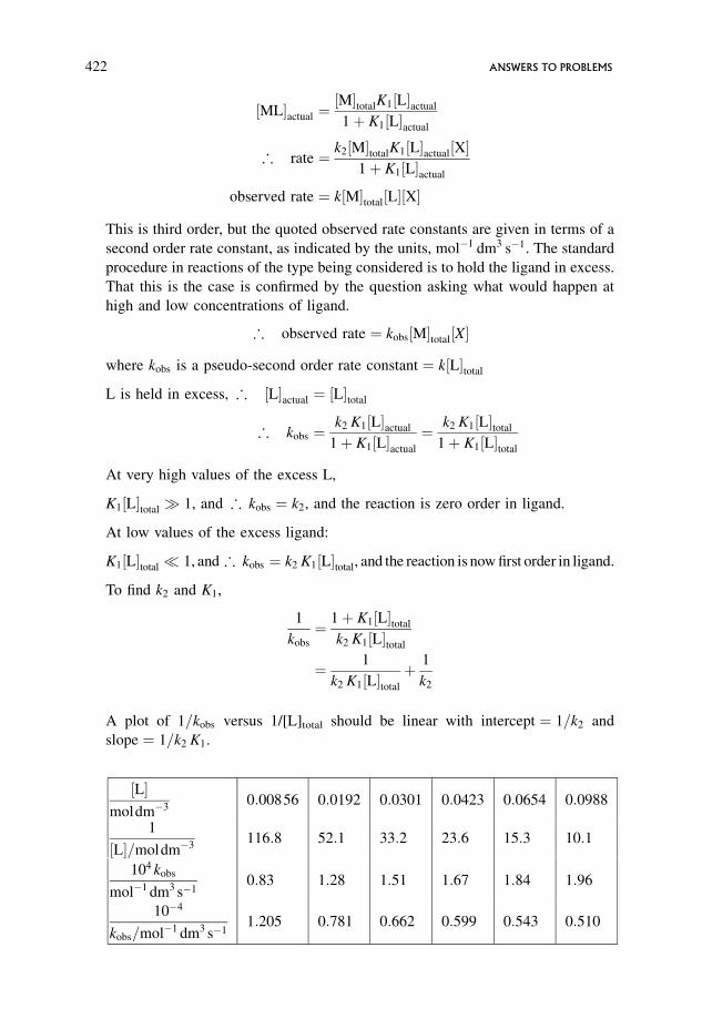
½ML�actual ¼½M�totalK1½L�actual
1þ K1½L�actual
; rate ¼ k2½M�totalK1½L�actual½X�1þ K1½L�actual
observed rate ¼ k½M�total½L�½X�
This is third order, but the quoted observed rate constants are given in terms of a
second order rate constant, as indicated by the units, mol�1 dm3 s�1. The standard
procedure in reactions of the type being considered is to hold the ligand in excess.
That this is the case is confirmed by the question asking what would happen at
high and low concentrations of ligand.
; observed rate ¼ kobs½M�total½X�
where kobs is a pseudo-second order rate constant ¼ k½L�total
L is held in excess, ; ½L�actual ¼ ½L�total
; kobs ¼k2 K1½L�actual
1þ K1½L�actual
¼ k2 K1½L�total
1þ K1½L�total
At very high values of the excess L,
K1½L�total � 1, and ; kobs ¼ k2, and the reaction is zero order in ligand.
At low values of the excess ligand:
K1½L�total � 1, and; kobs ¼ k2 K1½L�total, and the reaction is now first order in ligand.
To find k2 and K1,
1
kobs
¼ 1þ K1½L�total
k2 K1½L�total
¼ 1
k2 K1½L�total
þ 1
k2
A plot of 1=kobs versus 1/[L]total should be linear with intercept ¼ 1=k2 and
slope ¼ 1=k2 K1.
½L�moldm�3
0:00856 0:0192 0:0301 0:0423 0:0654 0:0988
1
½L�=moldm�3116:8 52:1 33:2 23:6 15:3 10:1
104 kobs
mol�1 dm3 s�10:83 1:28 1:51 1:67 1:84 1:96
10�4
kobs=mol�1 dm3 s�11:205 0:781 0:662 0:599 0:543 0:510
422 ANSWERS TO PROBLEMS
The graph is linear confirming the kinetic analysis:
intercept ¼ 1=k2 ¼ 0:43 104 mol dm�3 s ; k2 ¼ 2:33 10�4 mol�1 dm3 s�1
slope ¼ 1=k2 K1 ¼ 0:66 102 mol2 dm�6 s ; K1 ¼1
k2 0:66 102
¼ 65 mol�1 dm3
7. (a) rate of reaction ¼ k2½ML5�actual½L��actual
½ML6�total ¼ ½ML6�actual þ ½ML5�actual
K1 ¼½ML5�actual½L�actual
½ML6�actual
and ½ML6�actual ¼½ML5�actual½L�actual
K1
We need to find ½ML5�actual in terms of ½ML6�total and K1.
½ML6�total ¼½ML5�actual½L�actual
K1
þ ½ML5�actual
¼ ½ML5�actual
½L�actual þ K1
K1
� �
½ML5�actual ¼ ½ML6�total
K1
½L�actual þ K1
� �
; rate of reaction ¼ k2½ML5�actual½L��actual
¼ k2 K1½ML6�total½L��actual
½L�actual þ K1
Since L� is held in excess, then the amount removed by reaction is very small
compared with ½L��total, ; ½L��actual � ½L��total
; rate ¼ k2 K1½ML6�total½L��total
½L�actual þ K1
observed rate ¼ kobs½ML6�total½L��total
kobs ¼k2 K1
½L�actual þ K1
Note: kobs here is a true second order rate constant.
Usually, with an equation having a denominator which is a sum or difference,
the reciprocal of both sides is taken:
1
kobs
¼ K1 þ ½L�actual
k2 K1
¼ 1
k2
þ ½L�actual
k2 K1
The standard graph would be a plot of 1=kobs versus [L]actual. This is not
possible since L is the product of the pre-equilibrium, which is not removed by
further reaction, and so builds up continuously throughout the reaction.
CHAPTER 8 423
(b) If L is held in excess by adding a known large excess, then ½L�actual ¼ ½L�total,
and values of kobs could be found for several experiments where a different
value of excess L is used for each. A plot of 1=kobs versus [L]total would then
be linear with intercept ¼ 1=k2 and slope ¼ 1=k2 K1. From these k2 and k1 can
be found individually.
8. (a) Since the equilibrium is set up rapidly and is maintained throughout reaction,
the slow step is step 2, and
rate of reaction ¼ k2½adduct�actual½Br2�actual
K1 ¼½adduct�actual
½alkene�actual½Br2�actual
and ½alkene�actual ¼½adduct�actual
K1½Br2�actual
½alkene�total ¼ ½alkene�actual þ ½adduct�actual
¼ ½adduct�actual
K1½Br2�actual
þ ½adduct�actual
¼ ½adduct�actual
1þ K1½Br2�actual
K1½Br2�actual
� �
½adduct�actual ¼ ½alkene�total
K1½Br2�actual
1þ K1½Br2�actual
� �
rate ¼ k2 K1½Br2�2actual½alkene�total
1þ K1½Br2�actual
observed rate ¼ kobs½alkene�total½Br2�2total
Note: the observed rate is second order in Br2, since the reaction involves, in
effect, one molecule of alkene and two molecules of Br2.
Since Br2 is in excess, ½Br2�actual � ½Br2�total
rate ¼ k2 K1½Br2�2total½alkene�total
1þ K1½Br2�total
; kobs ¼k2 K1
1þ K1½Br2�total
(b) If the Br2 excess is small, then K1½Br2�total � 1, and
rate � k2 K1½alkene�total½Br2�2total, and reaction is second order in Br2.
If the Br2 excess is large, then K1½Br2�total � 1, and
rate � k2½alkene�total½Br2�total, and reaction is first order in Br2.
(c)kobs ¼
k2 K1
1þ K1½Br2�total
1
kobs
¼ 1þ K1½Br2�total
k2 K1
¼ 1
k2 K1
þ ½Br2�total
k2
424 ANSWERS TO PROBLEMS
A plot of 1=kobs versus ½Br2�total should be linear with intercept ¼ 1=ðk2 K1Þand slope ¼ 1=k2. Hence k2 and K1 can be found.
(d) If K1 is very small, then K1½Br2�total � 1, and kobs ¼ k2 K1. Unless K1 is
known independently, k2 cannot be found.
9.
� d½H2A�total
d t¼ kuncat½H2A�total þ kcat½ZnA�actual
� d½H2A�total
d t¼ kobs½H2A�total
kobs ¼ kuncat þ kcat
½ZnA�actual
½H2A�total
¼ kuncat þ kcat K½Zn2þ�actual½A2��actual
½H2A�total
� �
since
K ¼ ½ZnA�actual
½Zn2þ�actual½A2��actual
The reaction is carried out at constant pH and so the fraction of the acid ionized
to the dianion, �, is constant throughout the experiment. Since the Zn2þ is in
excess then ½Znzþ�actual � ½Znzþ�total, giving
kobs ¼ kuncat þ kcat K �½Zn2þ�total
where
� ¼ ½A2��actual
½H2A�total
If the mechanism is correct and the approximations justified, a plot of kobs versus
[Zn2þ]total should be linear with slope ¼ kcat K � and intercept ¼ kuncat.
The graph is linear with intercept ¼ kuncat ¼ 0:725 10�4 s�1 and slope ¼ kcat
K � ¼ 1:475 10�2 mol�1 dm3 s�1.
Since K ¼ 1580 mol�1 dm3 and
� ¼ ½A2��actual=½H2A�total ¼ 6 10�5=0:03 ¼ 0:002 00; then
kcat ¼1:475 10�2 mol�1 dm3 s�1
1580 mol�1 dm3 0:002 00
¼ 4:67 10�3 s�1
CHAPTER 8 425
Index
Bold type indicates definitions
A factor 93, 104, 108–109, 136–137,
138–140, 140, 143–144, 265–267, 289,
293, 294, 295, 297, 298, 299, 300, 339
determination of 104, 108, 349
Absorbance 8, 8–13, 20, 29
Absorption coefficient, molar 8, 11
Absorption of radiation 2, 7, 8–9, 13, 14, 15,
19, 20, 204–206
Absorption of sound 35–38
Accelerated flow 29
Acid catalysed hydrolysis 26, 75, 331–336
Acid–base catalysis 359, 365
Activated complex 4, 100, 125–127, 129,
130, 131, 132, 224
degrees of freedom 135, 137–139, 143–145
in unimolecular theory 155, 158–159,
160–161
thermodynamic aspects 140–142, 143–145
with respect to PE surfaces 165–168, 169,
171–180
statistical mechanical aspects 132–139
reactions in solution 265, 267, 269–272,
281, 284, 289, 292, 293, 294,
296–297, 297–300, 303–304, 305,
306, 308–309, 310–313, 329,
331–332, 335–336
structure, reactions in solution 331–332,
335–336
Activated intermediate 129–130, 132
Activated molecule 2–3, 122, 129, 147–148,
152, 153, 154, 155, 156, 158, 159,
160–161, 196, 223
Activating collision 3, 153
Activation 2, 3, 4, 87–89, 122, 135, 147, 148
in unimolecular reactions 152–153,
153–154, 155, 157, 158–160
in complex gas reactions 185, 196–198,
222–223, 224, 227–229, 235
in reactions in solution 293, 296,
297–300, 302, 303–304, 304,
308–309, 310–313
Activation energy 2, 92–95, 103, 104–108,
134, 136, 156–158, 224, 227, 238–239,
255–257, 267–268, 303–304
determination of 92–95
calculations using 104–108
see also critical energy
Activity 270–271, 342
Activity coefficient 270–271, 271–272
Actual and total concentration 89–90,
284–285, 321–328, 330–331, 332–336,
336–339, 340–341, 341–342, 342–343,
344–346, 346–351, 352–356, 356–358,
360–363, 363–365, 365–368
Actual ionic strength 284–285
Adsorption at surface 240–243
Angle of scattering 110–112, 112–122
Angular velocity 103
Anharmonicity 124–125, 161, 228
Anion catalysis 317, 334, 334–336
‘‘Approach to equilibrium’’ 66, 90
Arrhenius 2
Arrhenius equation 92–95, 100, 103,
104–106, 108–109, 136, 154–159,
161, 279–280, 339
Association 264, 281, 284–285, 289, 313
An Introduction to Chemical Kinetics. Margaret Robson Wright# 2004 John Wiley & Sons, Ltd. ISBNs: 0-470-09058-8 (hbk) 0-470-09059-6 (pbk)
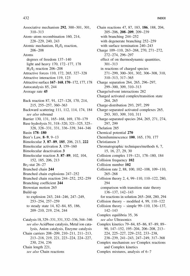
Associative mechanism 292, 300–301, 301,
310–313
Atom–atom recombination 160, 214,
228–229, 240, 243
Atomic mechanism, H2/I2 reaction,
206–208
Atoms
degrees of freedom 137–140
light and heavy 170, 172–177, 178
H2/I2 reaction 206–208
Attractive forces 110, 172, 265, 327–328
Attractive interaction 119, 123
Attractive surface 167–168, 170–172, 177, 178
Autocatalysis 85, 244
Average rate 45
Back reaction 87, 91, 127–128, 170, 214,
215, 255–257, 360–363
Backward scattering 111, 112, 114, 174, 184
see also rebound
Barrier 130, 131, 165–168, 169, 170–179
Base hydrolysis 51, 318–320, 321–325, 325–
328, 328–331, 331, 336–339, 344–346
Basin 178–180
Beer’s Law, 8–9, 9–13
Bimolecular 3, 87–89, 185, 206, 213, 222
Bimolecular activation 3, 159–160
Bimolecular deactivation 3
Bimolecular reaction 3, 87–89, 102, 104,
152, 185, 206, 213
Br2-stat 26–27
Branched chain 244
Branched chain explosions 247–252
Branched chain reaction 244–252, 252–259
Branching coefficient 244
Brownian motion 265
Build-up
to explosion 243, 244–246, 247–249,
253–254, 257–259
to steady state 14, 82–84, 85, 186,
209–210, 219, 234, 244
Catalysis 18, 329–331, 331, 332–336, 344–346
see also Acid/base catalysis, Metal ion cata-
lysis, Anion catalysis, Enzyme catalysis
Chain carriers 208–209, 210–211, 211–213,
213–218, 219, 221, 223–224, 224–227,
230, 234, 236
Chain length 221,
see also Chain reactions
Chain reactions 47, 87, 183, 186, 188, 204,
205–206, 208–209, 209–239
with branching 244–252
with degenerate branching 252–259
with surface termination 240–243
Charge 109–110, 263–268, 270, 271–272,
272–274, 296–297
effect of on thermodynamic quantities,
301–313
in reactions of charged species
271–299, 300–301, 302, 306–308, 310,
310–313, 317–365
Charge separation 264, 265, 296–297,
299–300, 309, 310–313
Charge/solvent interactions 282
Charged activated complex/transition state
264, 265
Charge-distribution 293, 297, 299
Charge-separated activated complexes 265,
293, 303, 309, 310, 311
Charge-separated species 264, 265, 271, 274,
297, 299
Chelation 285
Chemical potential 270
Chemiluminescence 100, 165, 170, 177
Christiansen 3
Chromatographic techniques/methods 6, 7,
15, 16, 27, 29, 30
Collision complex 119–121, 178–180, 184
Collision frequency 102
Collision number 102
Collision rate 2, 88, 100, 102–108, 109–110,
265–268
Collision theory 2, 4, 99–110, 110–122, 280,
294
comparison with transition state theory
136–137, 142–143
for reactions in solution 265–268, 280, 294
Collision theory – modified 4, 99, 110–122
Collision theory – simple 99–110, 136–137,
142–143
Complex equilibria 35, 36
see also Ultrasonics
Complex kinetics 79–84, 85–86, 87–89, 89–
90, 147–152, 195–204, 206–208, 213–
224, 225–227, 229–232, 233–238,
238–239, 241–243, 247–249, 317–368
Complex mechanism see Complex reactions
and Complex kinetics
Complex mixtures, analysis of 6–7
432 INDEX
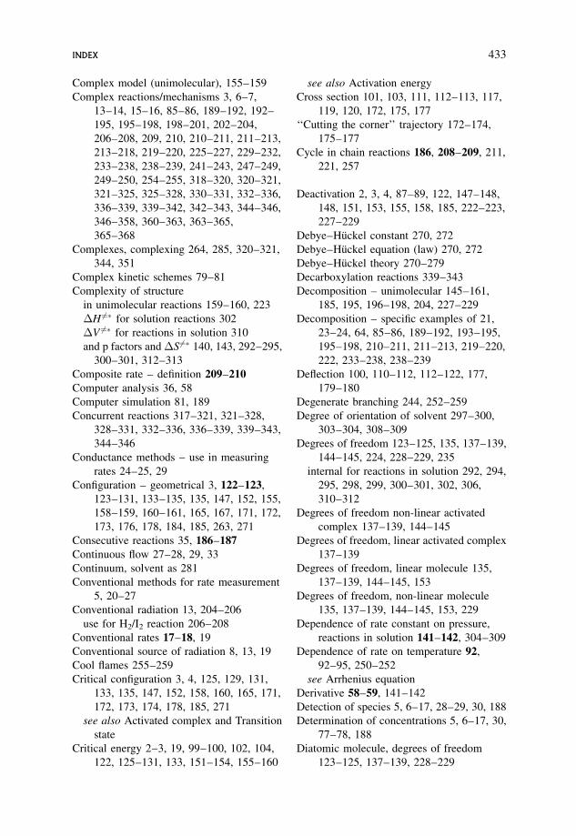
Complex model (unimolecular), 155–159
Complex reactions/mechanisms 3, 6–7,
13–14, 15–16, 85–86, 189–192, 192–
195, 195–198, 198–201, 202–204,
206–208, 209, 210, 210–211, 211–213,
213–218, 219–220, 225–227, 229–232,
233–238, 238–239, 241–243, 247–249,
249–250, 254–255, 318–320, 320–321,
321–325, 325–328, 330–331, 332–336,
336–339, 339–342, 342–343, 344–346,
346–358, 360–363, 363–365,
365–368
Complexes, complexing 264, 285, 320–321,
344, 351
Complex kinetic schemes 79–81
Complexity of structure
in unimolecular reactions 159–160, 223
�H 6¼� for solution reactions 302
�V 6¼� for reactions in solution 310
and p factors and �S6¼� 140, 143, 292–295,
300–301, 312–313
Composite rate – definition 209–210
Computer analysis 36, 58
Computer simulation 81, 189
Concurrent reactions 317–321, 321–328,
328–331, 332–336, 336–339, 339–343,
344–346
Conductance methods – use in measuring
rates 24–25, 29
Configuration – geometrical 3, 122–123,
123–131, 133–135, 135, 147, 152, 155,
158–159, 160–161, 165, 167, 171, 172,
173, 176, 178, 184, 185, 263, 271
Consecutive reactions 35, 186–187
Continuous flow 27–28, 29, 33
Continuum, solvent as 281
Conventional methods for rate measurement
5, 20–27
Conventional radiation 13, 204–206
use for H2/I2 reaction 206–208
Conventional rates 17–18, 19
Conventional source of radiation 8, 13, 19
Cool flames 255–259
Critical configuration 3, 4, 125, 129, 131,
133, 135, 147, 152, 158, 160, 165, 171,
172, 173, 174, 178, 185, 271
see also Activated complex and Transition
state
Critical energy 2–3, 19, 99–100, 102, 104,
122, 125–131, 133, 151–154, 155–160
see also Activation energy
Cross section 101, 103, 111, 112–113, 117,
119, 120, 172, 175, 177
‘‘Cutting the corner’’ trajectory 172–174,
175–177
Cycle in chain reactions 186, 208–209, 211,
221, 257
Deactivation 2, 3, 4, 87–89, 122, 147–148,
148, 151, 153, 155, 158, 185, 222–223,
227–229
Debye–Huckel constant 270, 272
Debye–Huckel equation (law) 270, 272
Debye–Huckel theory 270–279
Decarboxylation reactions 339–343
Decomposition – unimolecular 145–161,
185, 195, 196–198, 204, 227–229
Decomposition – specific examples of 21,
23–24, 64, 85–86, 189–192, 193–195,
195–198, 210–211, 211–213, 219–220,
222, 233–238, 238–239
Deflection 100, 110–112, 112–122, 177,
179–180
Degenerate branching 244, 252–259
Degree of orientation of solvent 297–300,
303–304, 308–309
Degrees of freedom 123–125, 135, 137–139,
144–145, 224, 228–229, 235
internal for reactions in solution 292, 294,
295, 298, 299, 300–301, 302, 306,
310–312
Degrees of freedom non-linear activated
complex 137–139, 144–145
Degrees of freedom, linear activated complex
137–139
Degrees of freedom, linear molecule 135,
137–139, 144–145, 153
Degrees of freedom, non-linear molecule
135, 137–139, 144–145, 153, 229
Dependence of rate constant on pressure,
reactions in solution 141–142, 304–309
Dependence of rate on temperature 92,
92–95, 250–252
see Arrhenius equation
Derivative 58–59, 141–142
Detection of species 5, 6–17, 28–29, 30, 188
Determination of concentrations 5, 6–17, 30,
77–78, 188
Diatomic molecule, degrees of freedom
123–125, 137–139, 228–229
INDEX 433
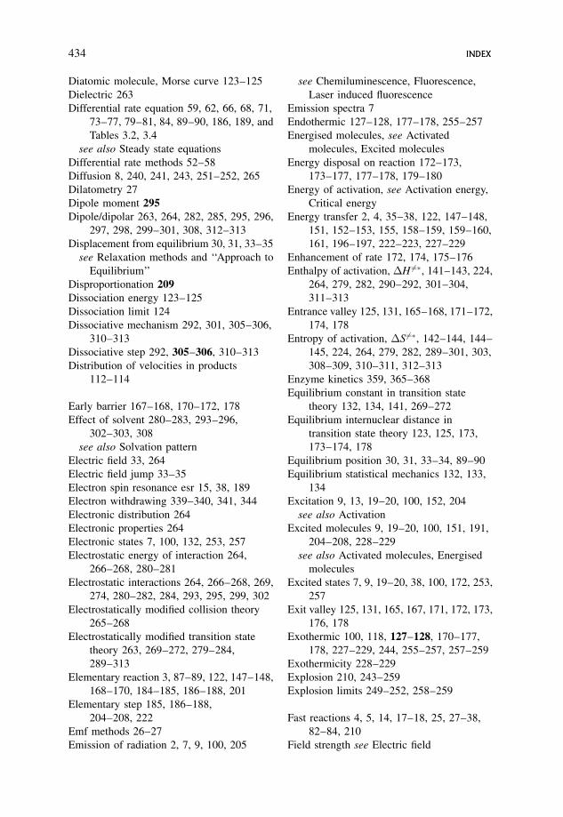
Diatomic molecule, Morse curve 123–125
Dielectric 263
Differential rate equation 59, 62, 66, 68, 71,
73–77, 79–81, 84, 89–90, 186, 189, and
Tables 3.2, 3.4
see also Steady state equations
Differential rate methods 52–58
Diffusion 8, 240, 241, 243, 251–252, 265
Dilatometry 27
Dipole moment 295
Dipole/dipolar 263, 264, 282, 285, 295, 296,
297, 298, 299–301, 308, 312–313
Displacement from equilibrium 30, 31, 33–35
see Relaxation methods and ‘‘Approach to
Equilibrium’’
Disproportionation 209
Dissociation energy 123–125
Dissociation limit 124
Dissociative mechanism 292, 301, 305–306,
310–313
Dissociative step 292, 305–306, 310–313
Distribution of velocities in products
112–114
Early barrier 167–168, 170–172, 178
Effect of solvent 280–283, 293–296,
302–303, 308
see also Solvation pattern
Electric field 33, 264
Electric field jump 33–35
Electron spin resonance esr 15, 38, 189
Electron withdrawing 339–340, 341, 344
Electronic distribution 264
Electronic properties 264
Electronic states 7, 100, 132, 253, 257
Electrostatic energy of interaction 264,
266–268, 280–281
Electrostatic interactions 264, 266–268, 269,
274, 280–282, 284, 293, 295, 299, 302
Electrostatically modified collision theory
265–268
Electrostatically modified transition state
theory 263, 269–272, 279–284,
289–313
Elementary reaction 3, 87–89, 122, 147–148,
168–170, 184–185, 186–188, 201
Elementary step 185, 186–188,
204–208, 222
Emf methods 26–27
Emission of radiation 2, 7, 9, 100, 205
see Chemiluminescence, Fluorescence,
Laser induced fluorescence
Emission spectra 7
Endothermic 127–128, 177–178, 255–257
Energised molecules, see Activated
molecules, Excited molecules
Energy disposal on reaction 172–173,
173–177, 177–178, 179–180
Energy of activation, see Activation energy,
Critical energy
Energy transfer 2, 4, 35–38, 122, 147–148,
151, 152–153, 155, 158–159, 159–160,
161, 196–197, 222–223, 227–229
Enhancement of rate 172, 174, 175–176
Enthalpy of activation, �H 6¼�, 141–143, 224,
264, 279, 282, 290–292, 301–304,
311–313
Entrance valley 125, 131, 165–168, 171–172,
174, 178
Entropy of activation, �S 6¼�, 142–144, 144–
145, 224, 264, 279, 282, 289–301, 303,
308–309, 310–311, 312–313
Enzyme kinetics 359, 365–368
Equilibrium constant in transition state
theory 132, 134, 141, 269–272
Equilibrium internuclear distance in
transition state theory 123, 125, 173,
173–174, 178
Equilibrium position 30, 31, 33–34, 89–90
Equilibrium statistical mechanics 132, 133,
134
Excitation 9, 13, 19–20, 100, 152, 204
see also Activation
Excited molecules 9, 19–20, 100, 151, 191,
204–208, 228–229
see also Activated molecules, Energised
molecules
Excited states 7, 9, 19–20, 38, 100, 172, 253,
257
Exit valley 125, 131, 165, 167, 171, 172, 173,
176, 178
Exothermic 100, 118, 127–128, 170–177,
178, 227–229, 244, 255–257, 257–259
Exothermicity 228–229
Explosion 210, 243–259
Explosion limits 249–252, 258–259
Fast reactions 4, 5, 14, 17–18, 25, 27–38,
82–84, 210
Field strength see Electric field
434 INDEX
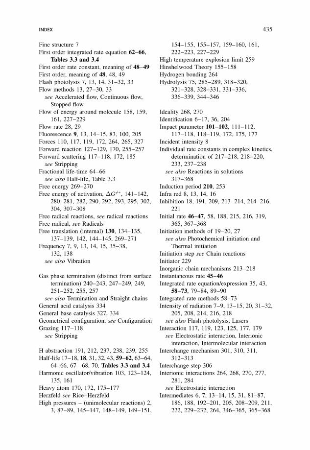
Fine structure 7
First order integrated rate equation 62–66,
Tables 3.3 and 3.4
First order rate constant, meaning of 48–49
First order, meaning of 48, 48, 49
Flash photolysis 7, 13, 14, 31–32, 33
Flow methods 13, 27–30, 33
see Accelerated flow, Continuous flow,
Stopped flow
Flow of energy around molecule 158, 159,
161, 227–229
Flow rate 28, 29
Fluorescence 9, 13, 14–15, 83, 100, 205
Forces 110, 117, 119, 172, 264, 265, 327
Forward reaction 127–129, 170, 255–257
Forward scattering 117–118, 172, 185
see Stripping
Fractional life-time 64–66
see also Half-life, Table 3.3
Free energy 269–270
Free energy of activation, �G 6¼�, 141–142,
280–281, 282, 290, 292, 293, 295, 302,
304, 307–308
Free radical reactions, see radical reactions
Free radical, see Radicals
Free translation (internal) 130, 134–135,
137–139, 142, 144–145, 269–271
Frequency 7, 9, 13, 14, 15, 35–38,
132, 138
see also Vibration
Gas phase termination (distinct from surface
termination) 240–243, 247–249, 249,
251–252, 255, 257
see also Termination and Straight chains
General acid catalysis 334
General base catalysis 327, 334
Geometrical configuration, see Configuration
Grazing 117–118
see Stripping
H abstraction 191, 212, 237, 238, 239, 255
Half-life 17–18, 18, 31, 32, 43, 59–62, 63–64,
64–66, 67– 68, 70, Tables 3.3 and 3.4
Harmonic oscillator/vibration 103, 123–124,
135, 161
Heavy atom 170, 172, 175–177
Herzfeld see Rice–Herzfeld
High pressures – (unimolecular reactions) 2,
3, 87–89, 145–147, 148–149, 149–151,
154–155, 155–157, 159–160, 161,
222–223, 227–229
High temperature explosion limit 259
Hinshelwood Theory 155–158
Hydrogen bonding 264
Hydrolysis 75, 285–289, 318–320,
321–328, 328–331, 331–336,
336–339, 344–346
Ideality 268, 270
Identification 6–17, 36, 204
Impact parameter 101–102, 111–112,
117–118, 118–119, 172, 175, 177
Incident intensity 8
Individual rate constants in complex kinetics,
determination of 217–218, 218–220,
233, 237–238
see also Reactions in solutions
317–368
Induction period 210, 253
Infra red 8, 13, 14, 16
Inhibition 18, 191, 209, 213–214, 214–216,
221
Initial rate 46–47, 58, 188, 215, 216, 319,
365, 367–368
Initiation methods of 19–20, 27
see also Photochemical initiation and
Thermal initiation
Initiation step see Chain reactions
Initiator 229
Inorganic chain mechanisms 213–218
Instantaneous rate 45–46
Integrated rate equation/expression 35, 43,
58–73, 79–84, 89–90
Integrated rate methods 58–73
Intensity of radiation 7–9, 13–15, 20, 31–32,
205, 208, 214, 216, 218
see also Flash photolysis, Lasers
Interaction 117, 119, 123, 125, 177, 179
see Electrostatic interaction, Interionic
interaction, Intermolecular interaction
Interchange mechanism 301, 310, 311,
312–313
Interchange step 306
Interionic interactions 264, 268, 270, 277,
281, 284
see Electrostatic interaction
Intermediates 6, 7, 13–14, 15, 31, 81–87,
186, 188, 192–201, 205, 208–209, 211,
222, 229–232, 264, 346–365, 365–368
INDEX 435
see Steady state and Chain carriers
Intermolecular interactions 100, 110, 111
Internal degrees of freedom see Degrees of
freedom
Internal free translation see Free translation
Internal modes for reactions in solution 310,
311
see also Degrees of freedom
Internal motions 137, 138, 292, 299, 302, 306
see also Free translation
Internal states 7, 9, 100
Internal structure 110, 137, 294, 296, 298, 299
Inverse first order 50, 202–204
Ion pair 264, 284–285, 285–289, 328–331
Ion–dipole reactions 295
Ionic strength 19, 270, 271–279, 281,
284–289, 293, 329, 332, 342
Ion–ion reactions 7, 265–268, 269–272,
273–279, 279–289, 293–294, 296–298,
300–301, 302–304, 306–307, 308–309,
310–313
Ion–molecule reactions 7, 185, 271, 274,
280, 295, 296, 298–299, 302–303, 308,
309, 310–313
Kassel Theory 158–160, 161
Kinetic analysis 5, 31, 43–95, 346–358
Kinetic energy 102–103, 104, 123
see also Rotation, Translation, Vibration
Kinetic theory 102, 131, 133
Kinetically equivalent mechanisms 183, 189,
198–201, 206–208, 317, 328–331,
332–336, 363–365
Large perturbation 31–33
Laser photolysis 14, 19, 31, 32, 204
Laser-induced fluorescence 9, 100
Lasers 4, 9, 13, 13–14, 15, 19, 20, 31, 32, 33,
83, 100, 204
Late barrier 165, 167, 167–169, 172–177,
178
Life time 186
Light atoms 170, 172–175, 176
Like charge/sign 109–110, 268, 281,
293–294, 297–298, 300, 302, 304–307,
310, 311, 312
Lindemann Mechanism 3, 153–155
Line broadening 38
Line width 7, 38
Linear activated complex – degrees of
freedom see Degrees of Freedom, linear
activated complex
Linear approach/linear recession 123
Linear configuration 123
Linear molecule – degrees of freedom
see Degrees of freedom, linear molecule
Long chains approximation 215, 217, 220,
221, 229–232, 234, 236
Low pressure – unimolecular reactions 2–3,
88, 145–147, 148, 150, 159–160,
196–198, 222–223, 227–228, 229, 235
Low pressure surface termination 240,
251–252, 254
Lower explosion limit 251–252
Luminescence 252, 257, 258
Major intermediate 188
Major products 188, 189, 211, 211–212
Mass 102, 130, 132, 138, 170
Mass/charge ratio 6
Mass spectrometry MS 6–7, 17, 27, 29, 30,
189
Mass type 170, 172–177
see also Heavy atom, Light atom
Master mechanism 3, 87–89, 147–148,
151–160, 185, 222–223
Mathematically complex schemes 81
Maximum rate 47
Maximum scattering 113–114
Maxwell–Boltzmann distribution 2, 102–
103, 125, 154, 155–156, 157–158
Mechanism 2, 3, 5, 6
see Complex reactions
Medium 264, 282
Metal ion catalysis 317, 329, 331, 334,
344–346
Metal ion complexes 344, 345
Michaelis constant 368
Michaelis–Menten equation 368
Microscopic 4, 122, 281, 283, 289
Microscopically inhomogeneous 283
Microwave 7, 8, 13, 15
Mild explosions 252, 253, 254
see also Cool flames
Minimum energy path 4, 165, 172–173, 176
see Reaction coordinate
Minor product 6, 7, 188, 189, 191, 209, 211,
212, 221, 222
436 INDEX
Modified solvent–solvent interaction 268
Molar absorption coefficient 8, 11
Molar units 103, 139–140, 157, 289
Molecular beam contour diagrams 112–122,
180
Molecular beams 4, 13, 100, 110, 110–122,
151, 170, 172, 174, 176–177, 179–180,
206
Molecular dynamics 4
Molecular units 103, 139–140, 157, 289
Molecularity 3, 292, 301, 305–306
Molecule–molecule reactions in solution
296, 299–300, 310–312
Moment of inertia 138
Morse curve 123–125
Most probable route 125, 172–173, 176
see Minimum energy path, Reaction
coordinate
Most probable velocity in products 113–116,
117, 119
Multi-step relaxation equilibria 35
Negative activation energy 240
Negative temperature coefficient/dependence
253, 254, 259
Non-chain complex reactions in gas phase
189–192, 192–195, 195–198, 198–201,
206–208
Non-equilibrium position 30
see Relaxation methods
Non-explosive region in branched chain
reactions 247–249, 250–252,
258–259
Non-ideality 263, 268, 269–280, 280, 284,
334, 342
Non-linear activated complex – degrees of
freedom, see Degrees of freedom
non-linear activated complex
Non-linear molecule – degrees of freedom,
see Degrees of freedom non-linear
molecule
Non-radical intermediates in steady state
treatments 202–204, 359–363
Non-reactive collision 100
Non-steady state 14, 188, 209–210
see Build up, Explosions
Normal mode
in transition state theory 123, 132,
135, 144
in unimolecular theory 153, 155, 157,
158–159, 159–160, 160, 161
with reference to third bodies 224,
227–229, 233, 235
Normal mode of vibration 123, 132, 135,
144, 153, 155, 157, 158–159, 159–160,
160–161, 224, 227–229, 233, 235
Nuclear magnetic resonance, nmr 15, 38
Nuclear spin states 7
Numerical integration 81, 189
Observed activation energy in terms of EA’s
of individual steps 238–239
Oppositely charged, see Unlike charge
Order (entropy) 298
Order meaning of 48–50
Order, determination of
Differential methods 52–58
Integrated methods 58–84
Orientation of solvent 297–300, 303–304,
308–309
Oscillate/oscillatory reaction 85, 255–258
Oscillator 123–124, 135, 161
see also Vibrational modes
Overall order 48
Oxidation of hydrocarbons 229–232
see also Cool flames
p factor 108–109, 109–110, 136, 140,
142–143, 145, 295, 296, 298
p factors, A, �S 6¼� for gases 109–110, 136,
140, 142–143, 145
p factors, A, �S 6¼� for solution reactions
265, 294, 295, 296, 298
Parallel reactions 186–188
Partial derivative 141–142
Partial pressure in stoichiometry 23–24
Partition function 99, 132–133, 134–135,
135–136, 137–140, 142–143,
265, 269, 271
Partition function per unit volume 133, 135
Path-length 8
PE contour diagram see Potential energy
contour diagram, Entrance valley, Exit
valley
PE maximum 4, 125
PE profile 126–128, 129–130, 133, 165–180
Period of sound wave 35
Periodic (displacements) 30, 35–38
INDEX 437
Permittivity, see Relative permittivity
Perturbation 30, 31, 33–35, 66, 90
pH 26, 26–27, 51, 319–320, 323, 324,
325–328, 331, 337–339, 341, 342,
342–343, 345
Photochemical equivalence, law of 205
Photochemical initiation 19, 214, 216
Photochemical rate 216, 218
see H2/I2 reaction 206–208
Photochemistry (photochemical) 2, 19,
19–20, 30, 31–32, 33, 188, 189–192,
204–206, 206–208, 210, 214, 216, 218,
237, 238
Photoelectron spectroscopy 15–16
Photolysis 7, 13, 14, 19, 31–32, 33, 204,
218
pH-stat 26–27, 319, 331, 345
Physical mechanism 87–89, 147–148, 185,
222
see Master mechanism
Physical methods 21–27, 27–38, 79
Polarisability 263–264, 313
Polyatomic molecule or ion, degrees of
freedom 137, 153, 228–229, 294, 295
see also Degrees of freedom, linear
molecule and non-linear molecule
Polyatomic molecule PE surface 122
Position of equilibrium 33, 35, 255–257,
322
Potential energy 3, 4, 103, 122–131, 133,
134, 135, 154, 165–180, 264, 271, 285
Potential energy barrier 130, 165–168
Potential energy contour diagram 126, 129,
131, 165, 166, 167, 169, 171, 173, 174,
175, 176
Potential energy surface 3, 122–131, 133,
134, 135, 142, 165–180, 184, 271
Potential energy well 178–179
Pre-equilibrium 92, 201, 202–204,
346–358, 359–365
Pre-exponential factor, see A factor
Pressure jump 33–35
Pressure limits in explosions 250–252, 254
Primary process, photochemical 204–206
Product valley, see Exit valley
Propagation 185, 186, 205–206
Straight chains 208–239
Branched chains, 244–259
Pseudo order 66, 74–77
Pseudo rate constant 74–77, 245, 318, 320,
320–321, 351, 354, 355, 358
Pulsed laser 14, 29, 32
Pulsed radiolysis 32
Quadrupole 282
Quantum (of radiation) in photochemistry
204–206
Quantum mechanical calculations 2, 123,
165
Quantum mechanical tunnelling 129–130
Quantum unimolecular theory 159, 161
Quantum yield 189–192, 204–206, 210
Quenching 20
Radiation 2, 7–15, 15–16, 19, 19–20, 29,
31–33, 100, 204–206, 208
Radicals
detection and identification of 6, 7, 13–17,
19, 31–33, 204
generation of 19–20, 31–33, 204
in solution 264, 359
see also Chain reactions, Chain carriers
Raman spectra 7, 8
Rate constant
meaning of 48–50
determination, differential method 52–58
determination, integral method 58–84
Rate, meaning of 44–47
determination of 17–38
Rate equation
Differential, see Differential rate equation
Integrated, see Integrated rate equation
Rate expression, meaning of 48–50
Rate of activation in unimolecular reactions
147–148, 151–152, 153, 155, 157–158,
158, 159–160
Rate of branching 245–246, 257, 258
Rate of change of configuration 130, 131
Rate of collision, see Collision rate
Rate of deactivation in unimolecular
reactions 147–148, 151–152, 153–154,
155, 158, 159–160
Rate of initiation, see Steady state, Explosions
Rate of propagation, see Propagation, Steady
state
Rate of reaction step in unimolecular
reactions 147–148, 154, 155, 158,
159–160
438 INDEX
Rate of termination, see Steady state,
Explosions
Rate, dependence on temperature see
Dependence of rate on temperature,
Arrhenius equation
Rate-determining step 82–83, 87–89, 92,
148, 154, 159–160, 222, 227–228, 235,
240, 243, 346–347, 348, 352, 357
Reactant valley, see Entrance valley
Reaction coordinate 4, 125, 126, 127, 129,
130, 133, 134, 135, 165, 172, 176, 178
Reaction unit/Reaction entity 122, 123, 125,
126, 130, 131, 133, 165, 171, 173, 174,
176, 178, 263
Reactions in solution 19, 20, 21, 38,
141–142, 263–368
Reactive collision 103, 111–112
Rebound mechanism 118–119, 174, 184
Recycle, see Regeneration
Redistribution of energy 100, 155
Reduced mass 102, 105–106, 133–135
Regeneration of chain carriers 186, 188, 192,
193, 208, 209, 211, 212
Regeneration of catalyst 331, 332, 365
Relative permittivity 19, 263, 264, 265, 266,
267, 268, 269, 280–283, 285, 293, 295,
296, 299, 302, 303, 306 307, 308
Relative translational motion 102, 104, 152
Relative velocity 100–101
Relaxation methods 30–32, 32–38
Relaxation time 35–36, 64–66, Table 3.3
Repulsion 110, 119, 171, 178, 265
Repulsive barrier see Late barrier
Reversible reactions 81, 89–91, 92, 198–201,
202–204, 255–257, 257–258, 346–358,
359–368
Rice–Herzfeld Mechanisms 221–243
Rotation 7, 100, 103, 110, 119, 135, 137,
138–139, 140, 144–145, 153, 178–179,
224, 292, 294, 306
Rotational degrees of freedom 135, 137,
138–139, 144–145, 153, 224, 292, 294,
306
Rotational mode 103, 135, 144–145, 153
Rotational partition function 132, 135,
138–139, 140
Rotational state 7, 100
Rotational symmetry number 132
Rotational energy 153
Rotational structure 100, 294
Saturation 354
see Swamping
Scattered products 111, 111–122, 172,
174–175, 177, 178–180, 184
Scattering 100, 110–122, 172, 174–175, 177,
178–180, 184
Scattering diagram (long lived complex)
119–120, 178–180, 184
Second explosion limit 252
Second order meaning of 47–49
Second order integrated rate equation 66–68,
68, Table 3.4
Second order rate constant meaning of
47–49
Secondary process, photochemical 204–205
Self-heating 244, 252, 257–258
Shock tube 7, 13, 31, 33, 34
Simple model (unimolecular) 153–155, 157
Sine waves 161
Single impulse 30, 33–35, 90
Slater Theory 160–161
Small perturbation 30, 33–35, 35–38, 66
Solute/solute interactions 268
see also Ionic interactions
Solute/solvent interactions 268
Solvation 263, 267, 268, 269, 281, 282, 283,
285, 296–301, 303–304, 308–309, 310,
311, 312, 312–313
Solvation pattern 263, 269, 281, 296–301,
303–304, 308–309, 310, 311, 312,
312–313
Solvent/solvent interactions 263, 268
Sound wave 35–38
Specific base catalysis 329
Spectrophotometry 8–13, 14, 27, 29
Spectroscopic methods of analysis/
determination/estimation 6, 7–16,
19, 27, 29, 30, 31–32, 38, 132, 170,
204–206
Spectroscopic quantities used in statistical
mechanics 132, 135, 271
Spin resonance 15, 38
Squared terms 102–103, 154, 155–156,
157–158
Standard state 142, 307
Steady state conditions/region 84–89, 246,
247–249, 257
INDEX 439
Steady state method/treatment/analysis
84–89, 89, 147–149, 186, 192–195,
196–198, 198–201, 202–204, 207–
208, 213, 214–218, 218–221, 222,
225–227, 229–232, 233–238,
238–239, 241–243, 246, 247–249,
257, 359–360, 360–362, 362–363,
363–365, 365–368
Stoichiometric arguments 23–24, 77–79
Stoichiometric concentration 284–285
Stoichiometric ionic strength 284–285, 289
Stopped flow 28–29
Straight chain 208–239, 240–243
comparisons with Branched chain 244,
246, 247–248, 249–250, 254, 254–255,
255–257, 258–259
Stripping 117–118, 119, 120, 170–172, 177
Structureless continuum 281
Substrate in enzyme kinetics 365
Successful collisions 103, 111–112
Surface reactions 19, 210, 240–243,
247–249, 249, 251–252, 255, 257
Surface termination 210, 240–243, 247–249,
249, 251–252, 255, 257
Swamping 354
see Saturation
Symmetrical PE barrier 131, 165–167
Symmetrical PE contour diagram 131, 166
Symmetrical PE profile 131, 166–167
Symmetrical scattering 119–122
Symmetry number 132
Temperature effect of 1, 92–95, 100, 104–
108, 154–155, 157, 159, 160, 161, 250–
252, 254, 255–257, 257–259, 268, 339
see also Arrhenius equation
Temperature, effect on relative permittivity
293
Temperature jump 33–35
Temperature limit, cool flames 254,
258–259
Termination 208–239, 239–243, 243–259
Termolecular reaction 3, 87, 185, 199, 201
Thermal explosions 244
Thermal initiation 19–20, 216
Thermal rate, see H2/I2 reaction 206–208
Thermodynamic formulation of transition
state theory 140–145, 265, 269,
269–272, 279–313
Thermodynamic functions/quantities
140–142
Thermoneutral 127–128
Third bodies 183, 227–229, 241, 243
Third explosion limit 252
Third order meaning of 48, Table 3.4
Three-halves (3/2) order 48, and Table 3.2
Time lag 3, 147, 154, 158, 159
Total energy in transition state theory 123,
125, 129
Total molecular partition function 134
Trace 6, 188, 211, 212, 253
Trajectory 172–173, 176
Transition state 4, 125
see Activated complex
Transition state theory 4, 99, 122–145, 224,
237, 263, 265, 269–272, 279–284,
289–313
Transition state theory expression 132, 136,
269
Translational degrees of freedom 135, 137,
138–139, 144–145, 224
Translational energy 118, 119, 120, 172, 174,
175–177, 178, 179
Translational partition function 132,
134–135, 137, 138–139
Transmission coefficient 130, 133–134,
269
Tunable laser 13
Tunnelling 129–130
Ultrasonic relaxation techniques 35–38, 66
Ultraviolet 7, 8, 13, 14, 16
Undeflected molecules 111, 172
Unimolecular 2, 3, 87, 185, 222
Unimolecular theories 2, 99, 145,
145–161, 195
see Lindemann mechanism, Hinshelwood
theory, Kassel theory, Slater theory
Unimolecular reaction 2, 3, 19, 87, 99,
145–161, 185, 195–198, 222–223,
227–229, 233, 235, 240, 243, 292
Units 47, 49–50, 53, 55, 75–77, 95, 103,
107–108, 109, 139–140, 157–158, 289,
305, 318, 332–334, 354, 355, 358
Units of rate 47
Units of rate constants 49–50, 53
of pseudo rate constants 75–77, 318,
332–334, 354, 355, 358
440 INDEX
Unlike charge 265, 273–274, 281, 284,
293–294, 297–298, 302, 303, 307, 310,
311, 312, 327
Unscattered molecules 111, 172
Upper explosion limit 252
Velocity of sound 35–38
Vibration 103, 110, 118, 119, 120, 123–124,
125, 132, 135, 137, 138–140, 144–145,
151, 152–153, 153–161, 172, 174,
175–177, 178, 178–179, 224, 227–229,
235, 292, 302, 306
Vibrational degrees of freedom 103, 123–
124, 133, 135–137, 138–140, 144–145,
153, 153–161, 224, 227–229, 235, 292,
302, 306
Vibrational energy 103, 118, 119, 120,
123–124, 125, 151, 152–153,
153–161, 172, 174, 175–177,
178, 178–179
Vibrational frequency 132, 138
Vibrational modes 103, 123–124, 132, 135,
137, 138–140, 144–145, 153, 153–161,
224, 227–229, 235, 292, 302, 306
Vibrational states 7, 100, 151, 153–154, 155,
158–159
Vibrational structures 100
Viscosity 19, 263, 264
Visible radiation 7, 8, 13, 14, 31
Water rate 318–320
Wavelength 7, 8, 11, 13
Well 129–130, 131, 178–180
X-ray photoelectron spectroscopy 15–16
Zero ionic strength 274, 279, 280, 281, 282,
285, 293
Zero order meaning of 48–49
Zero order integrated rate equation 68–70.
Table 3.4
Zero order rate constant meaning of
48–49
INDEX 441
List of Specific Reactions Discussed
or Analysed as a Means of
Illustrating Various Points
Gas phase reactions
C2H5NH2 decomposition – calculation of rate constant from total pressure with time,
23–24
N2O decomposition – demonstration of first order kinetics from concentration with time
data, 64
C3H8 decomposition – formulation of steady state equations and prediction of rate
expression, 85–86
Cis/trans isomerisation of 1-ethyl-2-methylcyclopropane – example of finding the rate
constant for a reversible reaction, 91
Calculation of p factors for a variety of reaction types, 109–110
A unimolecular decomposition – calculation of observed first order plots from partial
pressure with time data, and illustration of the falling off in the first order rate constant
with decrease in pressure, 146–147
Cyclopropane isomerisation – demonstration of falling off in the first order rate constant
with decrease in pressure, 149–150, 150–151
Demonstration of the dependence of k1 on s for a unimolecular decomposition, 157–158
Photochemical decomposition of CH3COCH3 – deduction of a mechanism to fit experi-
mental observation, 189–192
Decomposition of di-2-methyl propan-2-yl peroxide – Formulation of steady state
equations and rate expression, 193–195
N2O5 decomposition – a steady state analysis, 195–198
Reaction of NO(g) with O2(g) – analysis and demonstration of kinetically equivalent
mechanisms, 198–201
The H2/I2 reaction in the gas phase – a mechanistic and kinetic analysis, 206–208
CH3OCH3 decomposition – determination of the mechanism, 210–211; the steady state
analysis, 219–220
An Introduction to Chemical Kinetics. Margaret Robson Wright# 2004 John Wiley & Sons, Ltd. ISBNs: 0-470-09058-8 (hbk) 0-470-09059-6 (pbk)
CH3CHO decomposition – determination of the mechanism, 211–213; the steady state
analysis, 233–238; setting up of the steady state expression for the overall activation
energy in terms of the activation energies for the individual steps, 238–239
H2/Br2 reaction – a steady state analysis on the reaction with inhibition, 213–216; without
inhibition 216–217; determination of the individual rate constants, 217–218
Stylised Rice-Herzfeld mechanisms, 221–224, with surface termination, 240–243
RH/Br2 reaction – a steady state analysis, 225–227
Oxidation of hydrocarbons – mechanism and steady state analysis, 229–232
A stylised branched chain mechanism – a steady state analysis, and kinetic criteria for the
explosive region, 246–249
H2/O2 reaction – an example of a reaction with explosion limits, 249–252
Cool flames in oxidation of hydrocarbons – an analysis of the chemical behaviour and
reactions involved, 254–259
Solution phase reactions
Hydrolysis of an ester – illustration of pseudo order, 75
CCl3COOH(aq) decarboxylation – demonstration of first order kinetics from volume of
CO2(g) produced with time, 77–79
Conversion of thiourea to ammonium thiocyanate – determination of activation energy
from experimental data, 93–95
Reaction of alkyl halides with anions in solution, RX(aq)þY�(aq), – a steady state
treatment and comparison with a pre-equilibrium treatment, 202–204, 360–363
Calculation of ionic strength 272–273
PtLXþ(aq)þY�(aq) – analysis of kinetic data demonstrating the primary salt effect,
277–279
CH2BrCOO�(aq)þ S2O2�3 (aq) – kinetic analysis on experimental data demonstrating
dependence of rate constant on relative permittivity, 282–283
(C2H5)3NþCH2COOC2H5(aq)þOH�(aq) – kinetic analysis on experimental data
demonstrating the primary salt effect, 285–289
V2þ(aq)þ Co(NH3)5SOþ4 (aq) – determination of �H 6¼ � and � S 6¼ � from rate constant as
a function of temperature, 290–291
Comment on magnitude and sign of �S 6¼� for a variety of reactions, 300–301
Determination of �V 6¼ � from dependence of rate constant on pressure, 304–305
Information deducible from the magnitude of �H 6¼�, �S 6¼� and �V 6¼� for a variety of
reactions 312–313
Comparison of �V 6¼� and �S 6¼� for a variety of reactions, 314
Base hydrolysis of an ester – deduction of the rate expression from the mechanism, 318–
320
Pt(dien)Clþ(aq)þ pyridine(aq) – analysis of experimental data in terms of a given
mechanism, 320–321
Base hydrolysis of glycine ethyl ester – mechanistic analysis and use of experimental
data to confirm the mechanism, an approximate analysis, 321–328; a full analysis,
336–339
428 LIST OF SPECIFIC REACTIONS
Base hydrolysis of an ester in presence of metal ions, metal ion catalysis – analysis in
terms of kinetically equivalent mechanisms, 330–331
Acid hydrolysis of a charged ester in the presence of SO2�4 (aq) anion catalysis – analysis
in terms of kinetically equivalent mechanisms, 332–336
Decarboxylation of �-ketomonocarboxylic acids – formulation of the rate expression
from the mechanism, 339–341
Decarboxylation of �-ketodicarboxylic acids – approximations to the overall rate
expression deduced from the mechanism, 341–342
Decarboxylation of oxaloacetic acid – contributions to the overall rate, 342–343
Glycine ethyl ester, metal ion catalysed hydrolysis, formulation of the rate expression,
344–346
A�! �B! C – a pre-equilibrium kinetic analysis and predictions, 347–351, 363–365
Aþ B�! �C! D – a pre-equilibrium kinetic analysis and predictions, 351–356, 363–
365
FeIIIðCNÞ3�6 (aq)þ CoII(edta)2-(aq) analysis of experimental data using the schematic
mechanism – Aþ B�! �C! D, 356–358
Enzyme mechanism analysis, Eþ S�! �ES�! �Eþ product, 365–368
LIST OF SPECIFIC REACTIONS 429