An interactive-graphic environment for automatic generation of decision trees

ELSEVIER Decision Support Systems 18 (1996) 117-134

D asa0'

An interactive-graphic environment for automatic generation of decision trees

Tanguy Kervahut ~, Jean-Yves Potvin a,b., a D~partement d'informatique et de recherche op~rationnelle. Universit~ de MontrEal, C.P. 6128, Succ. Centre-ville, MontrEal,

Qu~.,Canada H3C 3.17 Centre de recherche sur les transports, Uniuersit3 de MontrEal, C.P. 6128, Succ. Centrewille, Montreal, QuL,Canada H3C 3J7

Abstract

In this paper, a computerized assistant for the construction of decision trees is described. With this system, designers of automatic tree building algorithms can quickly and easily evaluate new algorithmic designs for solving specific decision problems. A generic algorithmic template, which is initialized by the designer of algorithms with his(her) own formulas, is the basic mechanism for creating new tree building algorithms. These algorithms can then be tested on different decision problems, using the interactive-graphic environment provided by the system.

Keywords: Decision trees; Inductive learning; Algorithmic design; interactive-graphic environment

1. Introduction

This paper describes a computerized assistant for the design of algorithms that automatically construct decision trees. These algorithms are members of a class of inductive techniques that learn classification procedures through examples [l]. Other well-known members of this class are neural network models [10,12] and genetic classifiers [3].

The system presented in this paper is based on a generic algorithmic template which is initialized by the designer of algorithms with his(her) own formulas, in order to obtain algorithmic behaviors that are fit to specific decision problems. The generic template unifies a large class of algorithms for generat-

" Corresponding author. Email: [email protected]

ing decision trees, and greatly facilitates the design of new algorithms, as well as improvements or modifications to known algorithms. The template is em- bedded within an interactive-graphic environment aimed at facilitating the testing of new algorithms and the analysis of their behavior on different decision problems. In fact, the whole system can be viewed as a workbench for quickly exploring and refining new algorithmic ideas. Once a good algorithm is identified for the problems at hand, the final task of writing specialized (and fast) code can be done with the assurance that the underlying algorithm is a good one.

The paper is organized as follows. First, the contribution of the system for computer-aided decision making is underlined. Then, the classical ID3 algorithm [6], as well as a useful generalization [2], are briefly described. In Sections 4 and 5, the generic algorithmic template is introduced, as well as the

0167-9236/96/$15.00 © 1996 Elsevier Science B.V. All fights reserved SSD! 0167-9236(95)00030-5

118 T. Keroahut, J.- Y. Powin / Decision Support Systems 18 (1996) 117-134

interactive-graphic environment provided to the designer of algorithms. Finally, illustrative decision problems are presented to underline the benefits of this system.

2. Contribution of this work

Since the introduction of the Decision Support System (DSS) concept, many successes have been reported in the literature [4,15-17]. However, a DSS is often designed with a specific application in mind, and many different types of systems have been implemented thus far. In particular, some DSSs stand as "traditional" support tools while others now take a more active part in the decision making process. For example, intelligent symbiotic and adaptive DSSs are currently the focus of intense research [5,13]. These systems support decision making by making inferences, by selecting appropriate heuristics, rules or models, and by suggesting possible solutions to a problem. These capabilities are implemented through machine learning methods that are either supervised or unsupervised. Supervised learning strategies re- quire the implication of an external agent during the learning process (e.g., to provide a target solution to the system). Among these methods, we find rote learning, instructional learning, and deductive learning. Conversely, unsupervised learning techniques can generate useful knowledge without benefiting from an external agent. Among the inductive techniques in this class, we find the algorithms for automatically generating decision trees from a set of decision examples.

In the broad spectrum of decision aids, the contribution of our system is two-fold. First, the system is intended to designers of algorithms (and not to end users). Hence, designers of algorithms are viewed as decision makers, because they must choose appropriate procedural components in order to solve a particular problem or class of problems. Since the current system supports the design of algorithms for automatically generating decision trees, this tool could be very useful for constructing intelligent DSSs. That is, a good tree-building algorithm for a particular class of decision problems could be designed with our system, and later incorporated within an intelligent DSS.

Second, the system is based on a model, known as the generic algorithmic template, which unifies and generalizes different methods for automatically generating decision trees. Through the initialization of the algorithmic template, a specific algorithm can be produced for a given problem or class of problems. Accordingly, there is no "built-in" algorithm within the system, but rather a broad spectrum of known (and yet unknown) tree-building algorithms. This approach is quite different from the traditional "black-box" approach, where the underlying problem-solving strategy is fixed once for all, so that only minor changes are allowed (e.g., modifications to parameter values). Although many good induction packages are now available on the market, like Ex- Tran, RuleMaster and C4.5, these packages are in- stances of the traditional "black-box" approach, because the basic algorithms cannot be interactively modified by the user.

Finally, it is worth noting that our system is really a support tool that does not provide any active aid to the user. That is, algorithms produced with this system are as good as the designer of algorithms who creates them, given the limitations of the generic algorithmic template.

3. Tree construction algorithms

In this section, a classical algorithm for generating decision trees is first presented. Then, a generalization of this algorithm is introduced. Finally, a means to process continuous attributes is discussed.

3.1. The ID3 algorithm [61

ID3 is a well known procedure for inducing classification trees from examples. Each example, with a

Example al al Class

el Vl I v:l cl

¢2 vl! V22 C2

¢~ Y12 .Y22 ¢~

e4 Vl~ v:~ cl

e~ vl~ v;i c~

¢6 Vl3 v22 ¢2

Fig. I. A set of examples for generat ing a decision tree.

T. Kervahut. J.-Y. Potvin /Decis ion Support Systems 18 (1996) 117-134 119

known classification, is described via a set of attribute values. Fig. 1 shows a typical set of examples. Here, each example is a member of class cl, c 2 or c 3, and is described with two discrete attributes, namely a I with values vtz, vl2, vl3, and a 2 with

values U21 , /)22, /)23" ID3 uses a set of examples, like the one shown in

Fig. 1, to generate a decision tree. The nodes of the decision tree are associated with different subsets of examples. During the tree-building procedure, the initial set of examples is recursively partitioned into smaller subsets of examples. An evaluation function, usually derived from an entropy or uncertainty mea- sure, is applied to the subsets of examples to assess their "quali ty". This function returns low entropy values for subsets of high homogeneity, that is, subsets whose examples are mostly members of the same class. In particular, a subset whose examples are all members of the same class has a null entropy (i.e., no uncertainty).

Starting with the root as the current node (which is associated with the whole set of examples), the ID3 algorithm can be described as follows.

(1) For each attribute not yet selected at the current node do the following: Evaluate the entropy of each subset of examples produced by splitting the set of examples at the current node along all possible attribute values. Then, combine these entropy values into a global entropy value.

(2) Select the attribute that minimizes the global entropy, and apply this attribute to create the children of the current node. A child node is created for each value of the selected attribute, and contains the subset of examples that share the same value.

(3) Recursively apply this procedure to the children of the current node. The procedure stops at a given node, when the node is homogeneous, or when all attributes have been used along the path to this node.

This procedure will now be applied to the set of examples of Fig. 1, using the following entropy formula:

E( S) = - E Ps.c,l°g2 Ps.c,, Ct~ C

where S--- the set of examples at the current node; C = the set of classes (or categories); Ps.ck = the

proportion of examples in set S belonging to class

C k • In order to evaluate the entropy of attribute a i, the

set of examples S is partitioned into subsets S u- Each subset Si~ contains the examples in S that share the same value v u for attribute av Then, the entropy values of the subsets Si~ are combined to provide a single global value associated with attribute ai, namely:

v,l~ domain(a~)

for each attribute ai,

where ]SI is the cardinality of set S. The selected attribute minimizes E(aoS). Using

the set of examples of Fig. 1, the following results are obtained at the root node.

S = {ex,e2,e3,e4,e5,e6}

C = {c 1,C2,c3}

A = {al,a2}

2 x E(S~ ) + E(a,,s) ,

+ x e ( s . )

2 = -g X ( - (0.51og20.5) - (0.51og20.5)

- (o.olog O.O))

+ x ( - (o.51og O.5)

- (o.51og O.5) - (O.Olog2O.O))

2 + ~ X ( - (O.Olog20.O)

-- ( 0 .0 log 20.0 )

-- ( 1.0log 21.0)) = 0.6666

2 3 E( a 2 ,S) = g X E( S2, ) + -g X E( $22 ) I + g x E($13) = 0.7925

Hence, attribute a t is selected and the children of the root are created accordingly. As shown in Fig. 2, one child is homogeneous (for a I ----Vii) and no more processing is needed. The two other children are not homogeneous, and the procedure is recursively applied to each one of them, using the remaining attribute a l. At the end, the full decision tree of Fig. 2 is created.

120 T. Keruahut. J.- Y. P owin / Decision Support Systems 18 (1996) 117-134

alffiVll a2=v22 C 2

I et.¢2.¢3 e4.eS.¢6 c )

a I t = V l ~ c| alfVl3 a2=v21

¢2

Fig. 2. Decision tree produced by ID3.

This tree encodes the following decision rules: if at = vtl then c3 if (a t = or2 and a 2 = /.122) or (a t = vt3 and a 2 -- V22) then c 2 if (a¿ = or2 and a 2 = v23) or (a t = vt3 and a 2 = v21) then c t This algbrithm is very sensitive to the entropy

formula. In this example, selecting attribute a 2 before a t would create a different tree. Consequently, it is possible to generate many different decision trees by modifying the entropy formula.

The quality of a decision tree is based on both its accuracy and complexity. The accuracy is assessed by providing new examples with known classes, and by comparing these classes with the classes predicted by the tree. The complexity is related to the shape and size of the tree. Obviously, for the same accuracy, simple trees are preferred over complex ones.

One major weakness of ID3 is that a node is created for each value of a given attribute. In some cases, an attribute can get a good global evaluation, even if its entropy is good only for a few values among all its possible values (recall that the entropy of an attribute is a weighted sum over all values). Consequently, only the nodes associated with meaningful values should be generated. A modification along these lines is proposed in [2]. This is the topic of the next section.

3.2. A general ized ID3

In [2], the authors use "phantom attributes", derived from the original attributes, to generate decision trees. To this end, they introduce a tolerance level parameter (TL), with a value between 1 and

infinity, to identify meaningful attribute values. The algorithm works in the same way as ID3, but the selection of an attribute now requires two steps.

(a) Creating the phantom attributes. For each attribute not yet selected at the current

node, the entropy associated with each attribute value is computed. The minimal entropy value, thereafter called Enrropymin, is recorded.

Using this minimal value, the following computa- tion is performed for each attribute a i.

for each value vii of attribute a i, if entropy(S~j) < Entropymin X TL, then value v~j

is added to the list of meaningful values of attribute

a i otherwise, value v,.j is added to the list of default

values of attribute a i (meaningless values) Then, a phantom attribute a~ is created. This

attribute has one value for each meaningful value of ai. and a single default value associated to the meaningless values of a i.

(b) Selecting a phantom attribute. The entropy formula is applied again on the phan-

tom attributes a~. The phantom attribute with minimum entropy is selected to expand the tree.

It is worth noting that this algorithm can be seen as a generalization of the ID3 algorithm. If the tolerance level TL is set to a large value, all attribute values qualify as meaningful values, and the phantom attributes a~ are the same as the original attributes a i. Consequently, the algorithm will behave as the ID3 algorithm. However, different types of behaviors are obtained by modifying the tolerance level.

3.3. Cont inuous attributes

The above algorithm can be further extended by allowing attributes with a continuous domain of values, as in C4 (which is based on ID3 [8,9]). Here, the domain of values is partitioned into non overlapping intervals. A boundary between two intervals is selected in order to split the set of examples into two different subsets: one subset contains the examples with a value smaller than or equal to the boundary, and the other subset contains the remaining examples. All the boundaries are evaluated in turn, using the entropy function, in order to find the best boundary.

T. Kervahut, J.-Y. Powin / Decision Support Systems 18 (1996) 117-134 121

For instance, if the weight of an object is considered in a decision problem, many different intervals of fixed length are created, ranging from 0 to some maximal weight. If the length of each interval and the maximal weight are set to 10 and 50, respec- tively, the following intervals are created: [0,10], [10,20], [20,30], [30,40], and [40,50]. Consequently, boundaries 10, 20, 30, or 40 can be used to split the current set of examples into two different subsets. Assuming that the best boundary is 10, the current set of examples would be divided into two subsets: one subset would include all examples with a weight value in the interval [0,10], and the other subset would include the remaining examples, with a weight value in the interval ]10,50]. It is worth noting that the subset associated with [10,50] can be considered later for further splitting, since boundaries 20, 30 and 40 are still available. Conceptually, four new attributes weight w, weight2o, weight3o, and weight~o are created from the single attribute weight.

The algorithmic framework of the next section is based on Cheng's algorithm, and includes the processing of continuous attributes. However, it extends Cheng's algorithm by allowing the introduction of user-defined formulas.

4. The generic algorithmic template

The generic algorithmic template provides a flexi- ble framework for designing and testing new tree building algorithms. The template is based on Cheng's algorithm, and includes various "'slots" to be filled by the designer of algorithms in order to create new algorithms. In the following, the algorithmic template is described. Then, various functions available to the user are defined.

4.1. The algorithmic template

For the sake of simplicity, the algorithm presented in this section is restricted to discrete attributes only. The full description, for both discrete and continuous attributes, may be found in Appendix 1 at the end of the paper. Note also that the functions and parameters in italic in the pseudo-code description must be defined by the designer of algorithms.

Notation

S = initial set of examples A a = set of discrete attributes v o = jth value of discrete attribute a~ Sij. = subset of examples with value vii for discrete

attribute a~

Generic algorithmic template

Main procedure (S)

Create the root Assign the whole set of examples S to the root Call Tree Expansion Procedure(root, A d)

Tree expansion procedure (node, A a ) Step 1. Check the stopping conditions

If Stopping predicate is True or the default stopping condition applies to the set of examples in node then

classify the node with Classification function and Exit

Step 2. Initialize the variables Entropymin ~ arbitrary large number

Step 3. Compute the minimum entropy For each attribute a i in A a do

For each value v,.j of attribute a i do evaluate Entropy(Sij) with Evaluation Function if Entropy(S;i) < Entropymin then

set Entropymin to Entropy(Si~) Step 4. Create the phantom attributes

For each attribute a~ in Ad do For each value v,.j of attribute a~ do

if Entropy(S/j) < Entropymin × TL then put v~j in the list L , of individual values of the phantom attribute a;

otherwise, put vjj in the list L~2 of default values of the phantom attribute a;

122 T. Kervahut, J.-Y. Potvin / Decision Support Systems 18 (1996) 117-134

Step 5. Validate the phantom attributes Remove any phantom attribute with no meaningful values (i.e., no values in the list Lil)

Step 6. Select a phantom attribute Select the best phantom attribute a s' with Selec- tion Function

Step 7. Expand the current node For each value vs2 in the list Ls~ do

create a child node assign the subset of examples Ssj to the child node

Create a child node for the list of default values Ls2, and assign the remaining examples to this node.

Step 8. Update the status of the selected attribute If Ls2 contains a single attribute value then

remove a s from Act otherwise

set the list of values of a s to Ls2 Step 9. Recursion

For each child node do call Tree Expansion Procedure(child node, A d)

4.2. User-defined functions and parameters

Within the above template, the designer can spec- ify the following functions and parameters:

(a) Evaluation function. This function evaluates the sets of examples, and is called in the first phase of the attribute selection process, when the phantom attributes are created. This function can also be called by the user within his(her) Selection Function, when a phantom attribute is selected (see below).

The Evaluation function has one parameter: the set of examples to be evaluated. The output of the function is a numerical value, namely the evaluation or entropy of the set.

(b) Selection function. This function selects a phantom attribute to further expand the tree. Typi- cally, the Selection function calls the Evaluation function, as defined in point (a).

The Selection function has two parameters: the set of examples and the list of phantom attributes available at the current node. It returns the best phantom attribute in the list.

(c) Stopping Predicate. This function is used to stop the expansion process at the current node. The conditions expressed in the predicate are added to the default stopping condition, which is to stop when

the node is homogeneous or when all available attributes have been used. Consequently, if the stopping predicate is set to NIL, only the default stopping condition applies.

This predicate has a single parameter, the set of examples in the current node, and returns either T (True) or NIL (False).

(d) Classification Function. This function puts a class label on a terminal node or leaf of the tree. The default behavior, which is applied when the function is set to NIL, is the following: if there is only one class in the node (i.e. homogeneous node), it returns this class, otherwise it returns NIL. Quite often, the classification function is based on the majority rule, and the selected class is the one with the largest number of examples in the node.

The Classification function has a single parameter, the set of examples in the leaf, and it returns a class.

(e) Tolerance Level (TL). This parameter is the threshold for identifying meaningful attribute values (see Section 3). It is set to a numerical value between 1 and infinity. If TL is set to NIL, it means infinity.

In order to create a specific tree building algorithm, only the above functions or parameter values need to be defined by the user. In the following sections, we show how classical tree building algorithms can be specified within the generic algorithmic template. To this end, some useful built-in functions for creating tree building algorithms are first introduced.

5. Initialization of the generic template

To facilitate the definition of new functions within the algorithmic template, a set of built-in primitives are available. These primitives can be used as building blocks in the construction of new function definitions, and are defined on top of the Common Lisp language [18]. Accordingly, the user of the system can avoid the primitives if he(she) wants so as to use the full power of the Common Lisp language.

The Common Lisp language was chosen for two main reasons. First, the availability of the Medley programming environment greatly facilitates the design of user-friendly interfaces. Second, and more importantly, the Common Lisp language can be in- terpreted (rather than compiled). Given that our sys-

T. Kervahut, J.-Y. Potvin / Decision Support Systems 18 (1996) 117-134 123

tem relies on the dynamic creation, modification and application of different algorithmic components, it is very important to avoid the compilation of the whole template after each modification. The Common Lisp language provides this flexibility.

The built-in primitives provided by the system can be divided into two classes, Access Functions and Utility Functions. They are briefly described below.

5.1. Access functions

Each entity within the system is implemented as an individual object, with its own set of characteristics. The main classes of objects are Attributes, Examples, and Nodes (of the decision tree). The access functions allow the user to get the value associated with any given characteristic of an object. There is a rich library of such functions in the system. We only give below a few examples. These functions are used in Section 5.3 and in Appendix 2.

P.PH-VALUES (phantom attribute) Return the list of values of phantom attribute (if it is a discrete attribute) P,PH-TYPE (phantom attribute).

Return DISCRETE or CONTINUOUS P.CHILDREN (node).

Return the list of children of node. P.NB-EX (node)

Return the number of examples in node P.EX (node).

Return the list of examples in node

5.2. Utility functions

These functions are useful to build decision trees, and are provided as primitives. We give below a few examples.

P.CLASSES 0. Return the list of classes or categories of the current decision problem

P.NBEX-CLASS (set, class) Return the number of examples in set with the specified class.

P.PH-SPLIT (set, phantom attribute). Return the list of subsets of examples created by splitting the set of examples, using the values of phantom attribute.

P.SUBSET (set, attribute, values)

Return the subset of examples in set with an attribute value in the list of values.

P.ENTROPY (set). Returns the entropy of the set of examples, using the ID3 formula.

5.3. ID3

In the following, we illustrate the initialization of the generic template to create the ID3 algorithm. As mentioned before, four different functions, as well as the TL parameter value, must be defined.

Evaluation Function. Here, we assume that the function defined by the user for evaluating a set of examples according to the ID3 formula is called EVAL-ID3. The definition of this function in Com- mon Lisp is given below.

(DEFUN EVAL-ID3 (SET) (P.ENTROPY SET) )

Hence, this function simply calls P.ENTROPY on SET. However, without the availability of P.ENT- ROPY as a built-in primitive, EVAL-ID3 could be implemented in the following way (with a lot of comments!).

(DEFUN EVAL-ID3 (SET) /create local variables NBEX, CLASSES, SUM and RATIO. Initialize NBEX and CLASSES/ (LET ((NBEX (LENGTH SET))

(CLASSES (P.CLASSES)) SUM RATIO) /set variable SUM to O/ (SETQ SUM 0) /iterate over the list of CLASSES with local variable C / (DOLIST (C CLASSES)

/compute proportion of examples in class c~ (SETQ RATIO (/(P.NBEX-CLASS SET C) NBEX)) / i f there are examples in class C then compute the entropy formula for this class and add it to SUM/ (IF (> RATIO O)

(SETQ SUM (+SUM (.-1 RATIO (LOG RATIO 2))))))

/return SUM, the final entropy value/ (RETURN-FROM EVAL-ID3 SUM)

124 7". Kervahut, J.-Y. Potvin / Decision Support Systems 18 (1996) 117-134

Obviously, this function definition requires some knowledge of Common Lisp, but the use of built-in functions (with the prefix P.) greatly facilitates the user's task. Here, the local variables NBEX, CLASSES, SUM and RATIO are first declared. NBEX is set to the number of examples in the set, while CLASSES is set to the list of classes in the decision problem. Then, the entropy is computed and the final value is returned in the RETURN-FROM statement (the entropy being stored in the SUM variable).

Since intermixing English comments and Lisp

code produces very long function definitions, we will restrict ourselves to English-like descriptions in the following. However, the Lisp code for each function can be found in Appendix 2 at the end of the paper.

Se lec t ion F u n c t i o n . In this example, the function defined by the user for selecting a phantom attribute is called SELECT-ID3. The definition of this user- defined function is given below.

SELECT-ID3 (SET of examples, PHANTOM-AT- TRIBUTES)

initialize BESTVAL with an an arbitrary large number;

m m

illl~ II

* * * UP TO NOV : ASTIGNATISN : YES TEAR : NORMAL

* *e AVAILABLE ATTR|GUTE8 : ABE : YOUNG NIOOLE-AGE OLD PREGCRIPTION : NYOPIA HYPERNETROPIA

* * . TEST : PRESCRIPTION

ms* NUNBER OF EXANPLE$ : G N# S AGE YOUNg PREGCRIPTION MYOPIA ASTIGMATZSN YES TEAR NORMAL CLAgGE HARD K# 7 AGE YOUNg PRESCRIPTION NYPERNETROPIA AST|GMAT|SN YES TEAR NORMAL CLAGSE HARD Ik t 11 AGE NIODLE-AOE PRESCRIPTION MYOPIA A$TIONATI$R YES TEAR NORNAL CLAgGE HARO N# 15 AGE NIOOLE-AOE PRESCRIPTION HYPERMETROPIA AGTIGMATIGM YEG TEAR NORMAL CLASSE NOTHING N# 19 AGE OLD PRESCRIPTION MYOPIA ARTIOMATIGN YE8 TEAR NORMAL CLASSE HARD 14# 23 AGE OLD PRESCRIPTION HYPERNETROPIA AGT|GMAT|SN YES TEAR NORNAL CLASS( NOTHING

Fig. 3. The main screen.

T. Kervahut. J.-Y. Potvin / Decision Support Systems 18 (1996) 117-134 125

for each PHANTOM-A'I'q'RIBUTE in PHAN- TOM-A'VI'RIBUTES do

set VAL to 0; for each value of PHANTOM-Aq'q'RIBUTE do:

identify the SUBSET of examples in SET with this attribute value;

( I sUBSETI VAL *-- VAL + I SETI ×

EVAL - FN ( SV SET) ) ;

if VAL is less than BESTVAL then set BESTVAL to VAL; set BESTATT to PHANTOM-A'I'I'RI- BIYlE;

end for return the best phantom attribute BESTA'I'T.

In this definition, ISI stands for the cardinality of set S and EVAL-FN refers to the name of the function stored in the Evaluation Function slot of the algorithmic template. Hence, the call to EVAL-FN with the argument SUBSET is equivalent to a call to EVAL-ID3 in this example.

Stopping Predicate. The user-defined Stopping Predicate is set to NIL (the default stopping criterion applies).

Classification Function. The user-defined Classi- fication Function is called CLASS-MAJORITY, and implements the "majority rule": the class selected is the one with the largest number of examples in the set.

CLASS-MAJORITY (SET of examples) set NBEX-MAX to 0; for each class C do

if the number of examples in class C within SET is greater than NBEX-MAX then

set CLASS-MAX to C; set NBEX-MAX to the number of examples in class C;

end for return CLASS-MAX;

Tolerance Level. The tolerance level is set to NIL (i.e., infinity).

Using this initialization, the behavior of ID3 is

obtained. Of course, many different behaviors can be produced by modifying the function definitions and the TL parameter value. In the last sections, we show how the system can be used to easily generate different trees.

6. An interactive-graphic environment

In order to be a valuable workbench for designing and testing tree building algorithms, our Lisp-based system was implemented within a rich interactive- graphic menu-driven environment. As mentioned before, the system exploits the Medley programming environment available on the Sun workstations. Fig. 3 shows a typical screen. The Promptwindow in the upper left corner shows warning messages to the user. The executive window just below, allows the user to interact with the Lisp interpreter. The large window in the upper right corner displays decision trees. Finally, the window just below displays various information about the decision trees.

The main menu under the Executive window contains the interactive commands. We now go through some of these commands in order to illustrate a typical working session with the system.

(a) LOAD SPECIFICATIONS. The first step is to load a specification file. This file identifies the various attributes, as well as their characteristics. For a continuous attribute, the characteristics are the domain's lower bound and upper bound, and the length of each interval within the domain. For a discrete attribute, it is the list of all possible values. The file also identifies the various classes or categories.

In Section 7, Fig. 6 shows the specification file CONTACT-LENSES.SPEC for the problem of deciding if a patient can wear contact lenses, and if he(she) can, what type of contact lenses is appropri-

Fig. 4. Algorithmic template.

126 T. Kervahut. J.- Y. Potvin / Decision Support Systems 18 (1996) 117-134

ate. There are four discrete attributes to describe a patient, and the three decision classes are: nothing (no contact lenses), soft lenses or hard lenses.

(b) LOAD EXAMPLES. A file of examples, associated with the above specification file, must be defined. This file contains the description of a set of examples. In Section 7, Fig. 6 shows the example

file CONTACT-LENSES.EX, which is associated with CONTACT-LENSES.SPEC.

(c) CREATE ALGORITHM. Once the decision problem is defined, the user can design his(her) tree building algorithm. That is, the generic algorithmic template can be initialized with user-defined functions.

l | | H ~ I

EVAL-GINI OK ,EVAL-ID3

(DEFUN EVAL-ID3 (8ET) ~p

p3

(LET ((NBEX (LENGTH SET)) (CLASSES (P,OLA88ES)) SUM RATIO)

(SETQ BUM 8) (DOLIST (C CLA88E8)

(BETQ RATIO (/ (P.NBEX-OLASS SET 0) NBEX))

(IF (> RATIO 8) (SETQ SUN (+ SUM (* - I RATIO (LOS RATIO 2))))))

(RETURN-FROM EVAL-ID3 SUN)))

Fig. 5. Evaluation function.

T. Kervahut, J.-Y. P otuin / Decision Support Systems 18 (1996) 117-134 127

When the CREATE ALGORITHM command is applied, the dialog window shown in Fig. 4 is displayed.

Three command buttons are found in the upper pan of the window: OK to confirm the current initialization of the template, CANCEL to go back to the previous initialization, and ALGORITHMS to access a list of previously stored initializations.

The lower pan of the window includes the functions and parameters to be defined by the user. In the dialog window, the names of the current user-defined functions appear in the large rectangular area beside Evaluation Function, Selection Function, Stopping Predicate and Classification Function. The definition associated with each user-defined function can be accessed and modified by clicking on the function name with the mouse.

For example, the window shown in Fig. 5 is displayed when EVAL-ID3 is chosen. Its definition is in the lower pan of the window. In the upper pan, a list of names of (previously) created evaluation functions is displayed. Here, two user-defined functions are available under the names EVAL-ID3 and EVAL-GINI. EVAL-ID3 encodes the entropy formula of ID3 (as described in the previous section). EVAL-GINI is the name of some other evaluation function. Note that the current function EVAL-ID3 is highlighted with a black triangle in front of its name.

In the upper right comer of the window, a menu offers different commands. Among these commands, EDIT is used to interactively edit the current function definition. Once modified, the new definition can be saved under the same function name, or under a new name, using the CREATE command.

The current evaluation function is available for generating decision trees as soon as the window is closed with the OK command. This is a great benefit of the Common Lisp language: there is no need to recompile and link function definitions before using them.

(d) RUN ALGORITHM. Once defined, the algorithm can be applied to the current set of examples to generate a decision tree. The resulting tree is displayed in the large window in the upper right comer (see Fig. 3). The black nodes are the leaves or terminal nodes and are labelled with a class. The white nodes are non terminals, and are labelled with the attribute used to generate their children.

(e) PRUNE. This command implements the pessimistic tree pruning algorithm [7]. The aim of this procedure is to reduce the size of a decision tree, without compromising its accuracy. It is mainly a built-in algorithm. However, the user can modify the value of the pessimistic correction for the misclassi- fication rate.

(f) TEST. This command tests the current tree with new examples (with known classification). Af- ter specifying the name of an example file, each example is processed in turn by the tree and its classification is compared with the real classification. Statistics are provided in the information window (like the proportion of correctly classified examples).

7. A simple decision problem

This section shows how the system can be used to generate different decision trees for a simple decision problem. The problem consists of deciding if a person can wear contact lenses and if he(she) can, what type of lenses is appropriate.

Four attributes are used to describe a patient, as shown in the specification file of Fig. 6: age (young,

SPECIFICATION FILE: CON"rACI'-LENSES SPEC

ATI'R/BUTES

DISCRETE AGE 3 yOUNG NrlDDLE-ADE DISCRETE pRESCRIPTION 2 MYOPIA H YPER),IETROPIA DISCRETE ASTIGMATISM 2 YES DISCREI'E TEAR 2 NORMAL BELOW-NOR.MAL

CLASSES

NOTHING HARD SD~T

F2(ANfPLE FILE: CONTAC-I'-LILNSES EX

I YOUN~ MYOPIA 1~) BELOW-NORM ,.LL NOTHING 2 YOUNG MYOPIA NO NORMAL SOFT 3 YOUNG MYOPIA YES BELOW-NOR.M.M. N(YrH~G 4 YOUNG MYOPIA YES NORMAL HARD 5 YOUNG HYPERMETROPIA ,M3 BELOW-NOR_M M- NOTtl/NG 6 YOUNG HYPERMETROPIA ,NO NORMAL SOFT 7 YOUNG H YPERMETROPIA YES BELOW-NOILMAL NOTHL~G B YOUNG HYPERMETROPIA YES NORMAL HARD 9 MIDDLE.AGE MYOPIA ND BELOW-NOIZMAL NOTHING l0 MIDDLE-AGE MYOPIA NO NORMAL SOFT 11 MIDDI..E-AGE MYOPIA YES BELOW-NORMAL NOTH'~G 12 MIDDLE-AGE MYOPIA YES NORMAL tlARD 13 MIDDLE-AGE HYPEP, METROPIA NO BELOW-NOR.M AL NOTHING 14 MIDDLE-AGE HYPERMETROPIA NO NOR.MAL SOF'r 15 MIDDLE-AGE HYPERMETROPIA YES BELOW-NOILM M. NO'I'HI~G 16 MIDDLE-AGE H YPER.METROPIA YES NORMAl. N OTI4"LN G 17 OLD MYOPIA NO BELOW-NORMAL NOTHING Ig OLD MYOPIA NO NORMAL NOTHING 19 OLD MYOPIA YES BELOW-NORMAL NOTHING 20 OLD MYOPIA YES NORMAl. HARD 21 OLD HYPERMETROPIA NO BELOW-NORMAL NOTHING 22 OLD HYPERMETROpIA NO NORMAL SOFT 23 OLD H ~ T R O P I A YES BELOW-NORMAL NOTH1NG 24 CLD H ~ E R M E T R O P I A YES NORMAL NOTHLNG

Fig. 6. Specification file and example file.

Off)

128 T. Keruah ut, J.- Y. Potuin / Decision Support Systems 18 (1996) 117 - 134

A ~ = O ~ ~ Nothing

_ _ ~ ~ ~ - . Noth,ng

Age=Y ~ Soft

Fig. 7. Decision tree generated with Ib3.

middle-age or old), prescription (myopia or hypermetropia), astigmatism (yes, no) and tear production rate (normal, below-normal). The three decision categories are: nothing (no contact lenses), hard lenses and soft lenses. The set of examples for inducing the decision trees is also listed in Fig. 6.

Fig. 7 shows the decision tree generated by ID3, as specified within our algorithmic template (c.f., Section 5). In this figure, the values for attribute Tear are N = Normal, B N = Below-Normal; attribute As stands for Astigmatism; attribute Pr stands for Prescription with values H = Hypermetropia, M = Myopia; finally, the values of attribute Age are Y = Young, M = Middle-age, O = Old.

In order to generate a different tree, the formula for evaluating the entropy of attribute a i was modified as follows:

E( a,,S) "ew

vO~ domain(a~)

vijE domain(ai)

This modification is proposed in [6], and is aimed at reducing the bias of ID3 in favor of attributes with a larger range of values during the selection process. Hence, the function SELECT-ID3 was interactively modified (using the EDIT command), and the new

definition was saved under the name SELECT-ID3- NEW.

SELECT-ID3-NEW (SET of examples, PHAN- TOM-ATTRIBUTES)

initialize BESTVAL with an an arbitrary large number; for each PHANTOM-ATFRIBUTE in PHAN- TOM-ATrRIBU'I~S do

set NUMERATOR to 0; set DENOMINATOR to 0; for each value of PHANTOM-ATI~BUTE do

identify the SUBSET of examples in SET with this attribute value;

NUMERATOR

i ' I SUBSET[ <--- NUMERATOR V + I SET[

X EVAL - FN(SUBSET) ) ;

DENOMINATOR DENOMINATOR v

[ SUBSET[

+ ISETI

× LOG2 I SUBSETI I I SETI 1;

endfor

A g ~ Nothing

. . . . Pr=M ~ ~ - ~ . - m B I B Soft

Age=Y ~ Soft

Fig. 8. A decision tree produced with the new algorithm.

set VALto

T. Kervahut, J.-Y. Potvin / Decision Support Systems 18 (1996) 117-134

NUMERATOR

DENOMINATOR'

if VAL is less than BESTVAL then set BESTVAL to VAL; set BESTATI ~ to PHAN'IOM-ATTRI- BUTE;

endfor return the best phantom attribute BESTATr.

Using the new selection function SELECT-ID3- NEW, the tree shown in Fig. 8 was produced. Note that the test on the Prescription attribute is now applied before the test on the Age attribute in the lower part of the tree.

Here, both trees correctly classify all examples in the file of Fig. 6. Since this set of examples is exhaustive, both trees are equally accurate. In situa- tions where the set of training examples represent only a small sample of all possible examples (as it is usually the case), the trees generated by the user can be tested on additional examples with know classification, in order to identify the decision tree with the best generalization properties.

8. A more realistic application

This section presents another application of the system in the vehicle dispatching domain. Here, customers call a central dispatch office for some service (e.g., carrying express mail from one location to another in an urban area). After receiving a call, the dispatcher must choose a particular vehicle from a fleet of vehicles in movement to service the new request. Here, twelve attributes were used to describe the suitability of a vehicle for servicing a new request, like the vehicle's type, the distance between the current location of the vehicle and the location of the new request, the detour for servicing the new request, the service delay introduced in the planned route of the vehicle by the insertion of the new request (for other requests already allocated to this vehicle, but not serviced yet), etc.

Hence, the problem is to decide if a vehicle is suitable (or not) for servicing a request based on its current attribute description. Accordingly, only two classifications are possible for each vehicle: positive (suitable) or negative (not suitable). In this experi-

129

ment, the values of the numeric attributes were normalized between 0 and 1, and the unit interval was divided into ten non overlapping subintervals (see Section 3.3).

A file of service requests from a typical operations day was obtained from a courier service company operating in the city of Montreal. Based on this file, the evolution of the operations and the movement of the fleet of vehicles were simulated, using an interactive-graphic vehicle dispatching system [14]. During the simulation, a dispatcher identified the most suitable vehicle(s) for each new request. Although many vehicles could be identified as suitable for a given request, the dispatcher assigned only one vehicle at the end, so as to allow the simulation to proceed. At the end, 1,680 different attribute descriptions were available, as well as their classification. Given that only a fraction of the vehicles were suitable for each new request, the total number of negative examples was much larger than the total number of positive examples. Accordingly, the 380 positive examples were all kept, and 380 negative examples were randomly chosen. Then, the 760 examples were divided into three different training sets (each with 280 positive and 280 negative examples) and testing sets (each with 100 positive and I00 negative examples). The training and testing sets were obtained by selecting three disjoint sets of 100 examples for testing, and by using the remaining examples in each case for training.

Using our system, we tested ID3, ID3-NEW, and the GINI algorithm [1], which were all easily implemented within our algorithmic template. The resulting trees are very deep, even after the application of the pruning procedure, and are not shown here. However, the average performance of the pruned trees on the testing set are reported in Table 1.

Since most attributes are real-valued, the set of examples is often split in two along the boundaries

Table 1 Average % of correct classification on the testing sets of dispatching examples Class GINI ID3 ID3-NEW

Positive 86.3% 89.0% 89.3% Negative 83.6% 87.3% 87.3%

130 T. Kervahut. J.-Y. Powin / Decision Support Systems 18 (1996) 117-134

of the real domains. Accordingly, both ID3 and ID3-NEW were equally effective, with about 89% (87%) of correctly classified positive (negative) examples. GINI was outperformed by the two previous methods, but the percentage of correctly classified examples was still well over 80%. The best tree produced by ID3-NEW just happened to be the best tree over all methods and testing sets. It is character- ized by an early test on the service delay attribute, which measures the service quality, as well as the detour attribute, which measures the operations cost (e.g., a long detour implies high fuel consumption). This tree has since been incorporated within the vehicle dispatching system, in order to focus the attention of the dispatcher on the most interesting vehicles when a new request must be dispatched.

This example, and the previous example in Sec- tion 7, illustrate how the system can be used to quickly design different tree building algorithms for a particular decision problem. Here, we applied algorithmic ideas found in the literature, but any new idea that fits into the generic framework can be tested to produce different and (hopefully) better decision trees for a given problem.

9. Limitations of the system

The current system was not developed for com- mercial exploitation, and it still exhibits serious limitations that should be addressed in the future. First, the system does not support, uncertain or unknown data. This is a serious concern in many real-world problems, and different solution avenues based on probabilistic methods have already been proposed [8]. Another concern is the design of a common algorithmic framework for simplifying decision trees. This task is difficult, given that some algorithms simplify the decision tree at the same time as it is constructed (by deciding not to divide a subset of examples any further), while others prune the tree after it is constructed. Even among pruning algorithms, important discrepancies are observed. For example, the minimal cost-complexity pruning algorithm does not produce a single tree but rather a sequence of trees [1]; some pruning algorithms rely

on alternative testing sets to estimate the misclassifi- cation rate; etc.

With respect to the size of the problems that can be handled by the system, there is really no (practi- cal) limitations in terms of number of attributes per example or number of examples per application. This is related to the choice of the platform, a Sun workstation with a large virtual memory. However, it is clear that this choice, along with the choice of the Medley programming environment, greatly limit the number of potential users.

Finally, additional features like windowing, automatic rule production [9], and structured induction I1 l] could be implemented as well in the future.

10. Conclusion

The main contribution of this work concerns the development of a computer system that does not incorporate any built-in algorithm. Rather, the system offers a generic algorithmic template, from which a broad spectrum of user-defined tree construction algorithms can be created and tested on different decision problems.

Although the current system simply provides tools for quickly creating and testing new (or known) tree building algorithms, it would be interesting to develop an intelligent DSS or even an expert system in this domain. Such a system would take a specification file and an example file as input, and would suggest a good tree-building algorithm from a close analysis of the characteristics of the decision problem. We are still far from such a system, but our environment could help to develop this expertise by allowing the designers of algorithms to freely experi- ment with different algorithms.

Acknowledgements

Financial support for this work was provided by the Natural Sciences and Engineering Research Council of Canada (NSERC) and by the Quebec Fonds pour la Formation de Chercheurs et l'Aide h la Recherche (FCAR).

T. Kervahut, J.-Y. Powin / Decision Support Systems 18 (1996) 117-134 131

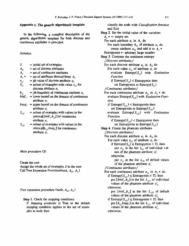
Appendix 1. The generic algorithmic template

In the following, a complete description of the generic algorithmic template for both discrete and continuous attributes is provided.

Notation

S Ad

Ac A c *

vij

sij

bij binf i

bsupi

si:

si:

= initial set of examples = set of discrete attributes = set of continuous attributes -- set of attributes derived from Ac = jth value of discrete attribute a i = subset of examples with value vii for

discrete attribute a~ = jth boundary of continuous attribute a i = lower bound on the domain of continuous

attribute a i -- upper bound on the domain of continuous

attribute a i = subset of examples with values in the

interval[ binfi,b~j] for continuous attribute a i

= subset of examples with values in the interval]b;j,bsup~] for continuous attribute a i

Main procedure (S)

Create the root Assign the whole set of examples S to the root Call Tree Expansion Procedure(root, An, A c)

Tree expansion procedure (node, A a, A c )

Step 1. Check the stopping conditions If Stopping predicate is True or the default stopping condition applies to the set of examples in node then

classify the node with Classification function and Exit

Step 2. Set the initial value of the variables A¢ * ~ empty set For each attribute a i in A c do

For each boundary bij of attribute a i do create attribute aij and add it to A c *

Entropymin *-- arbitrary large number Step 3. Compute the minimum entropy

/Discrete attributes/ For each discrete attribute a~ in A d do

For each value v~j of attribute a i do evaluate Entropy(Sij) with Evaluation Function if Entropy(Sij) < Entropymin then

set Entropymin to Entropy(Sly) /Continuous attributes/ For each continuous attribute aij in A c * do

evaluate Entropy(Siy I) with Evaluation Func- tion if Entropy(Sot) < Entropymin then

set Entropymin to Entropy(Sij 1) evaluate Entropy(Sly 2) with Evaluation Function

if Entropy(Sij 2) < Entropymin then set Entropymin to Entropy(So 2)

Step 4. Create the phantom attributes /Discrete attributes/ For each discrete attribute a i in A d do

For each value vii of attribute a i do if Entropy(Sij) < Entropymin × TL then

put vii in the list L,. I of individual values of the phantom attribute a~

otherwise, put vii in the list Li2 of default values of the phantom attribute a~

/Continuous attributes/ For each continuous attribute air in A c * do

if Entropy(Sij !) < Entropymin × TL then put [binfi,b~j] in the list L;j~ of individual values of the phantom attribute a::

otherwise, put [binfi,bij] in the list Lij ~ of default values of the phantom attribute a~j

if Entropy(Sij 2) < Entropymin × TL then put [bij.bsup~] in the list L;j I of individual values of the phantom attribute a:/

otherwise,

132 T. Kervahut. J.-Y. Powin / Decision Support Systems 18 (1996) 117-134

put ]b~j.bsuPi] in the list LO~ of default values of the phantom attribute ai~

Step 5. Validate the phantom attributes Remove any phantom attribute with no meaningful values (i.e., no values in the list L,. I or L~jl)

Step 6. Select a phantom attribute Select the best phantom attribute a~ (a'~,) with

Selection Function Step 7. Expand the current node

/Discrete attribute/ If discrete attribute a~ is selected then

For each value v# in the list Lst do create a child node assign to the child node the subset of examples Ssj

Create a child node for the list of default values Ls2 Assign the remaining examples to that node

/Continuous attribute/ If continuous attribute a't is selected then

Create two child nodes Assign the subset of examples Sst t to the first node Assign the subset of examples Sst 2 to the second node

Step 8. Update the status of the selected attribute /Discrete attribute/ If discrete attribute a ' is selected then

if Ls2 contains a single attribute value then remove a s from A d

otherwise set the list of values of a, to Ls2

/Continuous attribute/ If continuous attribute a" t is selected then

remove a, from A c if there is a boundary between binf s and b~t then

add attribute asl to A c set binf~l to binf~ and bsups t to b,t

if there is a boundary between b~t and bsups then

add attribute as2 to A c set binfs2 to bs~ and bsup, 2 to bsup,

Step 9. Recursion For each child node do:

call Tree Expansion Procedure(child node, A d, A c)

Appendix 2. Function definitions using Lisp code

In the current implementation of the system, function definitions must be written using Lisp code. Here, we provide the code for the functions EVAL- ID3, SELECT-ID3, CLASS-MAJORITY found in Section 5.3 and the function SELECT-ID3-NEW found in Section 7.

Section 5.3

EVAL-ID3: (DEFUN EVAL-ID3 (SET)

(EENTROPY SET) or

(DEFUN EVAL-ID3 (SET) (LET ((NBEX (LENGTH SET))

(CLASSES (P.CLASSES)) SUM RATIO) (SETQ SUM 0) (DOLIST (C CLASSES)

(SETQ RATIO (/(p.NBEX-CLASS SET C) NBEX)) (IF (> RATIO 0)

(SETQ SUM (+ SUM ( , - I RATIO (LOG RATIO 2))))))

(RETURN-FROM EVAL-ID3 SUM) )

SELECT-ID3 : (DEFUN SELECT-ID3 (SET PH-ATIRIBUTES)

(LET((NBEX (LENGTH SET)) (BESTVAL MOST-POSITIVE-FIXNUM) BESTATI" NBEX-SUBSET RATIO-SUB- SET VAL)

(DOLIST (PH-A'Iq" PH-AqTRIBUTES) (SETQ VAL 0) (DOLIST (SUBSET (P.PH-SPL1T SET PH- Arr))

(SETQ NBEX-SUBSET (LENGTH SUB- SET)) (SETQ RATIO-SUBSET ( / NBEX-SUB- SET NBEX)) (SETQ VAL

(+ VAL ( • RATIO-SUBSET (EVAL- FN SUBSET)))))

T. Keroahut, J.-Y. Powin / Decision Support Systems 18 (1996) 117-134 133

(IF ( < VAL BESTVAL) (SETQ BESTVAL VAL BESTA'I'r PH- ART)))

(RETURN-FROM SELECT-ID3 BESTATT)

(SETQ BESTVAL VAL BESTATr PH- A'IT)))

(RETURN-FROM SELECT-ID3 BESTATr)

CLASS-MAJORITY: (DEFUN CLASS-MAJORITY (SET)

(LET ((CLASSES (P.CLASSES)) NBEX-CLASS NBEX-MAX NBEX-CLASS)

(SETQ NBEX-MAX 0) (DOLIST (C CLASSES)

(SETQ NBEX-CLASS (P.NBEX-CLASS SET C)) (IF(> NBEX-CLASS NBEX-MAX)

(SETQ CLASS-MAX C NBEX-MAX NBEX-CLASS)))

(RETURN-FROM CLASS-MAJORITY CLASS-MAX)

)

Section 7

SELECT-ID3 -NEW: (DEFUN SELECT-ID3-NEW (SET PH-ATTRI- aLrrES)

(LET((NBEX (LENGTH SET)) (BESTVAL MOST-POSITIVE-FIXNUM) BESTATI" NBEX-SUBSET RATIO-SUB- SET NUM DENOM VAL)

(DOLIST (PH-ATr PH-ATrRIBUTES) (SETQ NUM 0 DENOM 0) (DOLIST (SUBSET (P.PH-SPLIT SET PH- Arr))

(SETQ NBEX-SUBSET (LENGTH SUB- SET)) (SETQ RATIO-SUBSET ( / NBEX-SUB- SET NBEX)) (SETQ NUM

(+ NUM ( • RATIO-SUBSET (EVAL- FN SUBSET))))

(SETQ DENOM ( + DENOM (* RATIO-SUBSET (LOG RATIO-SUBSET 2)))))

(SETQ VAL (/NUM DENOM)) (IF (< VAL BESTVAL)

References

[1] L. Breiman, J.H. Friedman, R.A. Olshen and C3. Stone, Classification and Regression Trees (Wadsworth, 1984).

[2] J. Cheng, U.M. Fayyad, K.B. lrani and Z. Qian, Improved Decision Trees: A Generalized Version of ID3, In: Proceed- ings of the Fifth International Conference on Machine Learn- ing (1988) 100-106.

[3] J.H. Holland, Adaptation in Natural and Artificial Systems (The MIT Press, 1992).

[4] P.G.W. Keen and M.S. Morton, Decision Support Systems: An Organizational Perspective (Addison-Wesley, NY, 1978).

[5] M.L. Manaheim, Issues in the Design of a Symbiotic DSS, In: Proceedings of HICSS-22, IEEE Computer Society (1988) 14-23.

[6] J.R. Quinlan, Induction of Decision Trees, Machine Learning 1 (1986) 81-106.

[7] J.R. Quinlan, Simplifying Decision Trees, lnemational Jour- nal of Man-Machine Studies 27 (1987) 221-234.

[8] J.R. Quinlan, Probabilistic Decision Trees, In: Y. Kodratoff and R. Michalski, Eds., Machine Learning: An Artificial Intelligence Approach, Vol. II1 (Morgan Kaufmann, 1990) 140-152.

[9] J.R. Quinlan, C4.5: Programs for Machine Learning (Morgan Kaufmann, 1993).

[10] D.E. Rumelhart and J.L. McClelland, Parallel Distributed Processing: Explorations in the Microstrncture of Cognition (The MIT Press, 1986).

[1 I] A.D. Shapiro, Structured Induction in Expert Systems (Ad- dison-Wesley, 1987).

[12] S. Schocken and G. Ariav, Neural Networks for Decision Support: Problems and Opportunities, Decision Support Sys- tems I I (1994) 393-414.

[13] M.J. Shaw, Guest Editor, Decision Support Systems I0, Special issue on Machine Learning Methods for Intelligent Decision Support (1993).

[14] Y. Shen, J.Y. Potvin, J.M. Rousseau and S. Roy, A Com- puter Assistant for Vehicle Dispatching with Learning Capa- bilities, Technical Report CRT-939, Centre de recherche sur les transports, Universitd de Montr6al.

[15] R.H. Sprague, A Framework for the Development of Deci- sion Support Systems, MIS Quarterly 4 (1980) !-26.

[16] R.H. Sprague and E.D. Carlson, Building Effective Decision Support Systems (Prentice-Hall, 1982).

[17] R.H. Sprague and H.J. Watson, Decision Support Systems: Putting Theory into Practice (Prentice-Hall, 1986).

[18] G.L. Steele, Common Lisp: The Language, Second Edition (Digital Press, 1990).

134 T. Kervahut. J.-Y. P owin / Decision Support Systems 18 (1996) 117-134

Jean-Yves Potvin is Associate Profes- sor at the Centre de recherche sur les transports and at the Department of computer science and operations research of Montreal University. He received a PhD degree in computer science from Montreal University in 1987. Then, he completed a postdoctoral fel- lowship at Carnegie-Mellon University in 1988. His current research interests are in the application of tabu search and genetic algorithms for solving complex

vehicle routing and scheduling problems.

Tanguy Kervahut received his MSc degree in computer science from the De- partment of Computer Science and Op- erations Research of Montreal Univer- sity in 1992. He is now working as programmer-analyst at Girt Inc., a software company specialized in vehicle routing and scheduling applications. He is involved in particular in the development of routing and scheduling software for municipal services and postal applications.

Documents

An interactive-graphic environment for automatic generation of decision trees