An Improved Group Contribution Method for the Prediction ofSecond Virial CoefficientsGiovanni Di Nicola,*,† Matteo Falone,† Mariano Pierantozzi,† and Roman Stryjek‡

†DIISM, Universita ̀ Politecnica delle Marche, Via Brecce Bianche 60131, Ancona, Italy‡Institute of Physical Chemistry, Polish Academy of Sciences, Warsaw, 01-224, Poland

*S Supporting Information

ABSTRACT: Techniques most commonly used for the estimation of the second virial coefficients are based on thecorresponding states principle. They are generally semiempirical correlating methods, and their validity is usually limited tononpolar gases or to small polar molecules. In this paper, an estimation technique for the second virial coefficients based on amodified group contribution method is presented. This method can be applied to a wide range of organic compounds. In fact, themethod depends on the knowledge of reduced temperature and acentric factor, and is based only on summing the products ofthe group contributions and their respective number of occurrences. Each group contribution is derived by analysis of the secondvirial coefficient data available in the literature.

■ INTRODUCTION

The deviation of real gas PVT behavior from the ideal gasequation of state shows that the knowledge of the PVTrelationship for real gases is needed. Many modifications of theperfect gas equation of state have been proposed to representthe PVT behavior of real gases, but the most satisfactory formregarding organic compounds at low and moderate pressures isthe virial equation of state.The following equation expresses the deviation from the

perfect gas equation as an infinite power series in V, the molarvolume:

= + + + +PVRT

BV

CV

CV

1 ...2 3 (1)

where B is the second virial coefficient, C is the third virialcoefficient, and D is the fourth virial coefficient. Even whentruncated at the second coefficient, the virial equation of stategives a remarkable estimate of the PVT relationship of realgases at low and moderate pressures (generally less than 1MPa). Because of this, estimation of second virial coefficients isan important task in thermodynamics. In addition, virialcoefficients are an important factor because they form a linkbetween the microscopic and macroscopic points of view,experimental results, and the knowledge of molecularinteractions. In fact, the second virial coefficient representsthe deviation from perfection due to interactions between pairsof molecules, the third virial coefficient reflects the effects ofinteractions of molecular triplets, and so on.Many theoretical or semiempirical models have been

proposed for second virial coefficients based on the theoreticalinterpretations of intermolecular interactions between mole-cules in the gaseous states. They are reasonably successful forsimple molecules. To overcome the limitations of theoreticaland semitheoretical models as applied to more complexmolecules, many empirical models were proposed in theliterature and they will be briefly described below.

Tsonopoulos1 modified the Pitzer−Curl’s equation2 toimprove its predictive capability. In particular, for nonpolargases, he introduced the following terms:

= − −−f T f T T( ) ( ) 0.000607TS

(0)r P C

(0)r r

8(2)

= + − −− − −f T T T T( ) 0.0637 0.0331 0.423 0.008TS(1)

r r2

r3

r8

(3)

He also introduced a corrective function to estimate the secondvirial coefficients of polar gases:

= −− −f T a T b T( )TS(2)

r T r6

T r8

(4)

where Tr is the reduced temperature, and aT and bT aretabulated parameters related to the reduced dipole moment, μr,of the compound studied. The final form of the Tsonopoulos’equation is

ω= = + +BPRT

f f T f T f T( ) ( ) ( )rc

B TS(0)

r TS(1)

TS(2)

r (5)

where Pc is the critical pressure (Pa) and ω is the acentricfactor.Vetere3 proposed a new version of the Pitzer−Curl’s

correlation.2 To this equation he added a new factor, ωV, andan additional term, f(2)(Tr), in which

ω = −T

M263V

b1.72

(6)

= − −

− −

− −

− −

f T T T

T T

( ) 0.1042 0.2717 0.2388

0.0716 0.0001502V

(2)r r

1r

2

r3

r8

(7)

Received: June 10, 2014Revised: August 18, 2014Accepted: August 18, 2014Published: August 18, 2014

Article

pubs.acs.org/IECR

© 2014 American Chemical Society 13804 dx.doi.org/10.1021/ie502334h | Ind. Eng. Chem. Res. 2014, 53, 13804−13809

Tb and M in eq 6 are, respectively, the normal boiling pointtemperature and molar mass. He obtained a correlation thatdescribes the temperature dependence of B for polar andnonpolar gases:

ω ω= = + +− −BPRT

f f T f T f T( ) ( ) ( )rc

B P C(0)

P C(1)

r V V(2)

r (8)

O’Connell and Prausnitz4 adopted both the first and the secondterms, f(0)(Tr) and f(1)(Tr), of the Pitzer−Curl’s correlation fornonpolar gases. For polar gases, they introduced two additionalfunctions, fμ(μr,Tr) and fa(Tr), based on the extended theory ofcorresponding states, in order to consider the polarity ofcompounds and their self-association trend. Their equation is

μ μ

μ μ

μ

μ μ

= − + −

−

+ −

+ −

μf T

T

( , ) 5.023722 5.65807(ln ) 2.133816

(ln ) 0.2525373(ln )

1/ [5.76977 6.181427(ln )

2.28327(ln ) 0.2649074(ln ) ]

r r r

r2

r3

r r

r2

r3

(9)

= −f T T( ) exp[6.6(0.7 )]a r r (10)

The O’Connell−Prausnitz’s complete equation reads asfollows:

ω μ η= + + +μ− −f f T f T f T f T( ) ( ) ( , ) ( )B P C(0)

r H P C(1)

r r r a r

(11)

where ωH is the acentric factor of the polar component’shomomorph and η is a constant of association for thecompound.Black5 suggested a van der Waals-type equation of state:

ξ= + −vRTP

ba

RT (12)

where ξ expresses the effects of temperature and pressure onthe molar cohesive energy.Starting from this equation of state, Black proposed a

correlation for B:

= + +BRT

Pf T f T

8( ) ( )a bC

CBL( )

r BL( )

r(13)

where:

= +

− + ′

− −

− −

⎜ ⎟⎛⎝

⎞⎠⎛⎝⎜

⎞⎠⎟f T

RTP

T T

T D T

( )2764

(0.396 1.181

0.864 )

BL(a)

rC

Cr

1r

2

r3

r4

(14)

= − ′ −⎛⎝⎜

⎞⎠⎟f T

RTP

E T( ) ( ) mBL(b)

rC

Cr

(15)

D′,E′, and m are adjustable parameters for polar compounds.Weber6 modified the Tsonopoulos’ correlation1 to better

describe the temperature dependence of the second virialcoefficients. He removed the last term in the Tsonopoulos’ eq2, and defined f TS

(1)(Tr) as follows:

= + −− −f T T T( ) 0.0637 0.0331 0.423TS(1)

r r2

r3

(16)

He also found a new method to calculate aT in theTsonopoulos’ function f TS

(2)(Tr).7 Weber obtained good results

introducing the aT function:

μ= − · −a 9 10T7

r2

(17)

In light of new data appearing in the open literature,especially for polar fluids such as haloalkanes, detailed analysison second virial coefficients predictions by the Tsonopoulosand Weber equations were performed.8,9 Important modifica-tions to the polar term were recently proposed,10 with aparticular attention to associated fluids, such as alcohols,amines, water, and quantum fluids.11 A different approach tofinding a correlation capable of estimating the second virialcoefficients is based on the group contribution method. Thebasic principle of this method is that every compound can bedivided into simpler subgroups and that these groupscontribute to the property examined. McCann and Danner12

proposed an equation capable of predicting the second virialcoefficients based on group additivity. Group contributionswere derived by analyzing available second virial coefficientdata, and are represented by the equation

Δ = + + + +B abT

cT

dT

eTi i

i i i i

r r3

r7

r9

(18)

For most groups, only the first four terms were required. Thesecond virial coefficients for any organic compound can becalculated from these group contributions and critical temper-atures, for reduced temperatures from 0.5 to 5, by summing upthe products of the group contribution (primary andsecondary) and their respective number of occurrences, n:

∑ ∑= Δ + − ΔB n B n B( 1)i i i ipri sec

2

(19)

The secondary group was defined only for the followinggroups: C−C2H2, C−C2F2, and Cb−F. In any case, the ΔBiterm, (cm3/mol), was calculated with eq 18 both for theprimary and the secondary group.

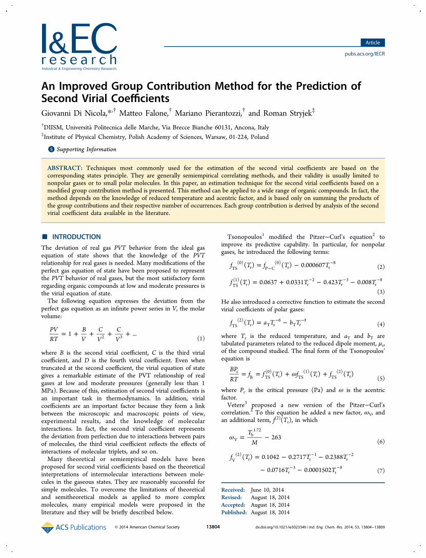
Figure 1. Histogram, data distribution, and statistical summary of the second virial coefficient experimental data.

Industrial & Engineering Chemistry Research Article

dx.doi.org/10.1021/ie502334h | Ind. Eng. Chem. Res. 2014, 53, 13804−1380913805

■ DEVELOPING THE NEW MODEL

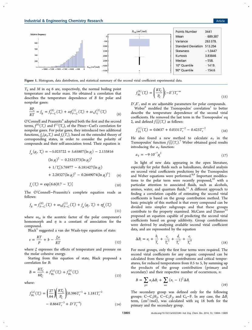
All estimation techniques generally need a large set ofexperimental data. In fact, through experimental data analysis,it is possible to find a function that describes the correlationbetween the second virial coefficients and the physical/molecular properties. Therefore, a data bank was created bycollecting experimental data on the second virial coefficientsavailable in the literature.13,14 It includes 3441 experimentaldata of second virial coefficients and their respectiveexperimental temperatures. Data were collected for 157compounds belonging to 19 families. In Figure 1, a statisticalsurvey of the data distribution of second virial coefficients isreported. From Figure 1, information on the data setdistribution and on the presence of the outliers inside thedata set are reported. Each datum lying outside the definedbounds can be considered as outlier. In our case, it is evidentthat the considered data are only out of the lower fence. Inparticular, 55 outliers were detected. All the experimental databy chemical family are shown in Figure 2, where the scatter plotof the second virial coefficients versus the reduced temperatureis reported. In Figure 2, a common behavior of the second virialcoefficients for all compounds present in the data bank isclearly evident. In particular, at low reduced temperatures, allvalues of B are widely negative, growing rapidly for reducedtemperatures close to unity. Then, the second virial coefficientsvalues slowly increase up to Boyle’s temperature. Informationon all data in the database is presented in Table 1, grouped byfamilies. For each group, the number of experimental data, therange of second virial coefficients, and the respective reducedtemperature range are summarized.This paper presents an estimation technique based on a

modified group contribution method for the second virialcoefficients developed by McCann and Danner,12 following theBenson group method.15 In fact, the proposed method startsfrom the Benson group contribution method based onsumming the products of the groups and their respectivenumber of occurrences as in eq 19, replacing eq 18 with a newequation containing the reduced temperature and the acentricfactor, ω, as follows:

ωΔ = + + + +⎛⎝⎜

⎞⎠⎟

⎛⎝⎜

⎞⎠⎟B a

bT

cT

de

Ti ii i

ii

r2

r4

r8

(20)

According to eq 20, the coefficients ai, bi, ci, di, and ei werecalculated for each group by a nonlinear regression fittingprocedure. Since the families of alkanes and aromatics werefound to be the most numerous in terms of data, their groupswere regressed separately. The obtained coefficients for alkanes

Figure 2. Scatter plot of the complete data set of second virial coefficients vs reduced temperature.

Table 1. Summary of Experimental Data for Each Family

nameno. ofpoints

no. ofcompounds

maximummolecularmass

Trrange

B range(cm3/mol)

acetates 66 4 102.13 0.61 to0.85

−2200 to−500

alcohols 179 10 102.17 0.55 to1.22

−3500 to−755

aldehydes 25 3 72.10 0.56 to1.02

−2210 to−260

alkanes 1121 16 114.22 0.55 to2.04

−2710 to−17.9

alkenes 415 13 112.21 0.48 to1.67

−2179 to−42.9

alkynes 62 4 54.090 0.59 to1.17

−1100 to−133

amines 100 10 101.19 0.55 to1.28

−2000 to−118

aromatics 500 13 186.055 0.48 to1.21

−2760 to−247

cycloalkanes 100 6 200.03 0.56 to1.60

−2050 to−82

cycloalkenes 5 1 68.12 0.66 to0.74

−820 to−630

dialkenes 40 4 68.12 0.56 to0.90

−1513 to−260.9

epoxides 25 4 88.10 0.52 to0.78

−1430 to−375

ethers 79 9 130.23 0.58 to0.93

−2650 to−306

formates 56 4 102.13 0.60 to0.81

−1738 to−440

haloalkanes 442 24 338.04 0.54 to1.31

−2320 to−106

haloalkenes 22 2 64.034 0.89 to1.40

−299 to−85.8

ketones 118 9 100.16 0.58 to0.93

−2860 to−400

mercaptans 28 9 116.22 0.56 to0.67

−1960 to−839

sulfides 58 12 112.19 0.53 to0.67

−2410 to−660

Industrial & Engineering Chemistry Research Article

dx.doi.org/10.1021/ie502334h | Ind. Eng. Chem. Res. 2014, 53, 13804−1380913806

and aromatics were then kept as fixed values during theregression of the complete set of data. As compared to theMcCann and Danner approach, the present method, besidesthe new reduced temperature dependence and the acentricfactor introduction as a parameter, considered a larger number

of fluids. In addition, four new groups were added, namelycyclopentene ring corrections, C−(CO)(C)3, Cb−(NI)(Cb)-(H), and Cb−(NI)(Cb)(C). To optimize the coefficients, theLevenberg−Marquardt curve-fitting method was adopted.16

This method is a combination of two minimization methods:

Figure 3. Scatter plot of absolute deviations vs reduced temperature for all the families excluding alkanes and aromatics.

Figure 4. Scatter plot of absolute deviations vs reduced temperature for alkanes and aromatics.

Figure 5. Scatter plot of relative deviations vs reduced temperature for all the families excluding alkanes and aromatics.

Industrial & Engineering Chemistry Research Article

dx.doi.org/10.1021/ie502334h | Ind. Eng. Chem. Res. 2014, 53, 13804−1380913807

the gradient descent method and the Gauss−Newton method.The Levenberg−Marquardt method acts more like a gradient-descent method when the parameters are far from their optimalvalue, and more like the Gauss−Newton method when theparameters are close to their optimal value and the solutiontypically converges rapidly to the local minimum. This way, itwas possible to identify the parameters of the proposedequation which guarantee the lowest deviation of the predictedvirial coefficients.The final equation proposed, even if very simple, produced

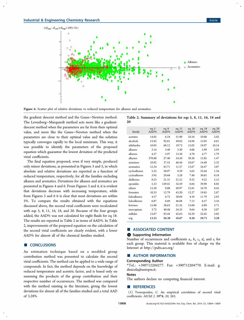
only minor deviations, as presented in Figures 3 and 5, in whichabsolute and relative deviations are reported as a function ofreduced temperature, respectively, for all the families excludingalkanes and aromatics. Deviations for alkanes and aromatics arepresented in Figures 4 and 6. From Figures 3 and 4, it is evidentthat deviations decrease with increasing temperature, whilefrom Figures 5 and 6 it is clear that most deviations are within5%. To compare the results obtained with the equationsdiscussed above, the second virial coefficients were recalculatedwith eqs 5, 8, 11, 16, 18, and 20. Because of the four groupsadded, the AAD% was not calculated for eight fluids for eq 18.The results are reported in Table 2 in terms of AAD%. In Table2, improvements of the proposed equation on the calculation ofthe second virial coefficients are clearly evident, with a lowerAAD% for almost all of the chemical families studied.

■ CONCLUSIONS

An estimation technique based on a modified groupcontribution method was presented to calculate the secondvirial coefficients. The method can be applied to a wide range ofcompounds. In fact, the method depends on the knowledge ofreduced temperature and acentric factor, and is based only onsumming the products of the group contribution and theirrespective number of occurrences. The method was comparedwith the method existing in the literature, giving the lowestdeviations for almost all of the families studied and a total AADof 3.28%.

■ ASSOCIATED CONTENT*S Supporting InformationNumber of occurrences and coefficients ai, bi, ci, di, and ei foreach group. This material is available free of charge via theInternet at http://pubs.acs.org/

■ AUTHOR INFORMATIONCorresponding Author*Tel.: +390712204277. Fax: +390712204770. E-mail: g.dinicola@univpm.it.NotesThe authors declare no competing financial interest.

■ REFERENCES(1) Tsonopoulos, C. An empirical correlation of second virialcoefficients. AIChE J. 1974, 20, 263.

Figure 6. Scatter plot of relative deviations vs reduced temperature for alkanes and aromatics.

Table 2. Summary of deviations for eqs 5, 8, 11, 16, 18 and20

familyeq 5AAD%

eq 8AAD%

eq 11AAD%

eq 16AAD%

eq 18AAD%

eq 20AAD%

acetates 14.05 6.18 51.90 18.16 10.80 2.92alcohols 12.85 92.61 49.02 14.94 15.03 6.61aldehydes 10.95 68.12 19.73 15.02 18.97 10.14alkanes 3.14 3.48 3.30 4.06 5.99 2.93alkenes 4.37 5.97 13.38 4.70 4.77 1.79alkynes 370.60 27.40 54.50 38.36 13.85 1.47ammines 10.92 37.55 46.56 10.67 14.40 2.32aromatics 12.34 83.71 11.57 13.67 16.47 3.87cycloalkanes 5.55 20.97 8.39 3.63 22.64 1.34cycloalkenes 3.95 29.68 5.28 7.48 30.65 0.18dialkenes 8.23 21.31 21.21 9.22 9.22 2.12epoxides 5.33 129.41 32.59 6.64 39.98 8.85ethers 12.50 9.08 49.97 12.81 16.70 8.42formates 10.33 12.79 43.20 12.27 19.85 2.87haloalkanes 4.57 6.72 30.84 4.34 11.79 2.83haloalkenes 6.87 6.69 46.68 7.13 8.57 3.16ketones 15.88 38.63 21.35 15.60 6.89 3.71mercaptans 3.72 40.48 54.35 9.64 8.38 2.07sulfides 12.07 83.44 42.63 16.29 22.62 5.02avg 13.51 26.38 18.67 8.26 10.71 3.28

Industrial & Engineering Chemistry Research Article

dx.doi.org/10.1021/ie502334h | Ind. Eng. Chem. Res. 2014, 53, 13804−1380913808

(2) Pitzer, K. S.; Curl, R. F. The volumetric and thermodynamicproperties of fluids. III. Empirical equation for the second virialcoefficient. J. Am. Chem. Soc. 1957, 79, 2369.(3) Vetere, A. An improved method to predict the second virialcoefficients of pure compounds. Fluid Phase Equilib. 1999, 164, 49.(4) O’Conell, J. P.; Prausnitz, J. M. Empirical correlation of secondvirial coefficients for vapour-liquid equilibrium calculations. IEC Proc.Des. Dev. 1967, 6, 245.(5) Black, C. Vapor phase imperfections in vapor−liquid equilibria.Ind. Eng. Chem. 1958, 50, 391.(6) Weber, L. A. Estimating the virial coefficients of small polarmolecules. Int. J. Thermophys. 1994, 15, 461.(7) Tsonopoulos, C. Second Virial Coefficients of Polar Haloalkanes.AIChE J. 1975, 21, 827.(8) Dymond, J. H. Second virial coefficients and liquid transportproperties at saturated vapour pressure of haloalkanes. Fluid PhaseEquilib. 2000, 174, 13.(9) Tsonopoulos, C. Second virial coefficients of polar haloalkanes−2002. Fluid Phase Equilib. 2003, 211, 35.(10) Meng, L.; Duan, Y. Y.; Li, L. Correlations for second and thirdvirial coefficients of pure fluids. Fluid Phase Equilib. 2004, 226, 109.(11) Meng, L.; Duan, Y. Y. An extended correlation for second virialcoefficients of associated and quantum fluids. Fluid Phase Equilib.2007, 258, 29.(12) McCann, D. W.; Danner, R. P. Prediction of second virialcoefficients of organic compounds by a group contribution method.IEC Proc. Des. Dev. 1984, 23, 529.(13) Dymond, J. H.; Marsh, K. N.; Wilhoit, R. C.; Wong, K. C. TheVirial Coefficients of Pures Gases and Mixtures. Landolt-Bor̈nstein;Springer: New York, 2002.(14) DIPPR-801, Project 801, Evaluated Process Design Data, PublicRelease Documentation, Design institute for Physical Properties (DIPPR);American Institute of Chemical Engineers, AIChE: New York, 2006.(15) Benson, S. W.; Buss, J. H. Additivity rules for the estimation ofmolecular properties. Thermodynamic properties. J. Chem. Phys. 1958,29, 546.(16) Marquardt, D. W. An algorithm for least-squares estimation ofnonlinear parameters. J. Soc. Ind. Appl. Math. 1963, 11, 431.

Industrial & Engineering Chemistry Research Article

dx.doi.org/10.1021/ie502334h | Ind. Eng. Chem. Res. 2014, 53, 13804−1380913809