Embed Size (px)
Citation preview

Atmos. Chem. Phys., 12, 3455–3478, 2012www.atmos-chem-phys.net/12/3455/2012/doi:10.5194/acp-12-3455-2012© Author(s) 2012. CC Attribution 3.0 License.
AtmosphericChemistry
and Physics
An extended Kalman-filter for regional scale inverse emissionestimation
D. Brunner1, S. Henne1, C. A. Keller1, S. Reimann1, M. K. Vollmer 1, S. O’Doherty2, and M. Maione3
1Empa, Swiss Federal Laboratories for Materials Science and Technology, Dubendorf, Switzerland2School of Chemistry, University of Bristol, Bristol, UK3Dipartimento di Scienze di Base e Fondamenti (DiSBeF), University of Urbino “Carlo Bo”, Urbino, Italy
Correspondence to:D. Brunner ([email protected])
Received: 27 September 2011 – Published in Atmos. Chem. Phys. Discuss.: 28 October 2011Revised: 17 February 2012 – Accepted: 2 April 2012 – Published: 11 April 2012
Abstract. A Kalman-filter based inverse emission estima-tion method for long-lived trace gases is presented for usein conjunction with a Lagrangian particle dispersion modellike FLEXPART. The sequential nature of the approach al-lows tracing slow seasonal and interannual changes ratherthan estimating a single period-mean emission field. Otherimportant features include the estimation of a slowly vary-ing concentration background at each measurement station,the possibility to constrain the solution to non-negative emis-sions, the quantification of uncertainties, the considerationof temporal correlations in the residuals, and the applica-bility to potentially large inversion problems. The methodis first demonstrated for a set of synthetic observations cre-ated from a prescribed emission field with different levels of(correlated) noise, which closely mimics true observations.It is then applied to real observations of the three halocar-bons HFC-125, HFC-152a and HCFC-141b at the remote re-search stations Jungfraujoch and Mace Head for the quan-tification of emissions in Western European countries from2006 to 2010. Estimated HFC-125 emissions are mostlyconsistent with national totals reported to UNFCCC in theframework of the Kyoto Protocol and show a generally in-creasing trend over the considered period. Results for HFC-152a are much more variable with estimated emissions be-ing both higher and lower than reported emissions in differ-ent countries. The highest emissions of the order of 700–800 Mg yr−1 are estimated for Italy, which so far does notreport HFC-152a emissions. Emissions of HCFC-141b showa continuing strong decrease as expected due to its controls indeveloped countries under the Montreal Protocol. Emissionsfrom France, however, were still rather large, in the range of
700–1000 Mg yr−1 in the years 2006 and 2007 but stronglydeclined thereafter.
1 Introduction
The atmosphere acts as an integrator in which emissionfluxes from individual sources get gradually mixed by at-mospheric transport processes. Atmospheric trace gas ob-servations therefore integrate information on a multitude ofsources, and it is the goal of inverse emission modeling toretrieve the original fluxes from individual sources (or usu-ally aggregated sources) by accounting for the effect of at-mospheric transport and mixing, and in case of reactive orsoluble gases for chemical conversion and removal. Inverseemission estimation is rapidly gaining in popularity as sev-eral studies have demonstrated its value for understandingnatural carbon fluxes (Houweling et al., 1999; Gurney et al.,2002; Rayner et al., 2008; Bousquet, 2009) and for evalu-ating classical “bottom-up” inventories (Bergamaschi et al.,2005; Chen and Prinn, 2006; Vollmer et al., 2009). Further-more, “top-down” emission estimation as provided by in-verse methods may provide up-to-date information for pol-icymakers to monitor the success of their emission reductionor mitigation measures.
Bottom-up inventories as compiled by individual nationsare typically obtained by combining emission factors for in-dividual processes with statistical information on the activityof those processes. Examples are the European EMEP Cen-tre on Emissions and Projections (CEIP,http://www.ceip.at/)inventory of atmospheric constituents relevant for human
Published by Copernicus Publications on behalf of the European Geosciences Union.

3456 D. Brunner et al.: Kalman-filter based emission estimation
health and ecosystems, or the United Nations FrameworkConvention on Climate Change (UNFCCC,http://unfccc.int)database of national greenhouse gas emissions. Despite largeefforts for homogenization of methods and validation, thereare considerable uncertainties involved in all steps of gen-eration of these inventories (Winiwarter and Rypdal, 2001)and many countries have only limited resources to collect thenecessary information. For the purpose of atmospheric mod-eling, spatially explicit, i.e. gridded inventories have beendeveloped such as the Emission Database for Global At-mospheric Research (EDGAR,http://edgar.jrc.ec.europa.eu/index.php) (Olivier et al., 2002).
There is a strong need for independent verification of in-ventories, particularly in the context of international treatieson climate, air quality, and the protection of the ozone layer.Previous studies have pointed out the great potential of top-down estimation of greenhouse gas emissions (e.g.,Houwel-ing et al., 1999; Bergamaschi et al., 2005; Bousquet et al.,2006; Rayner et al., 2008; Gockede et al., 2010; Hirsch et al.,2006) but they also revealed often large and poorly quantifieduncertainties associated with this approach (e.g.,Kaminskiet al., 2001; Engelen et al., 2006; Gurney et al., 2002; Linand Gerbig, 2005; Baker et al., 2006).
In this study we present an emission estimation approachgenerally applicable to long-lived or weakly reactive tracegases with only positive surface fluxes (emissions), i.e. tracegases with negligible deposition/uptake at the surface. Themethod is demonstrated for halocarbons which are measuredquasi-continuously at only few sites in Europe, and the abil-ity to invert emissions on a country-by-country basis is ex-plored. Chlorinated and brominated halocarbons includingchlorofluorocarbons (CFCs) and bromocarbons (halons) areharmful to the ozone layer and have therefore been bannedunder the Montreal Protocol (World Meteorological Organi-zation, 2007). They have first been substituted by hydrochlo-rofluorocarbons (HCFCs) which have shorter lifetimes andtherefore lower ozone depletion potentials (ODPs). HCFCsare currently being replaced by chlorine-free hydrofluoro-carbons (HFCs) with zero ODP. However, like CFCs andHCFCs these HFCs are often potent greenhouse gases con-tributing to global warming and are therefore included in theKyoto Protocol. Without further regulation, their continuedgrowth in the atmosphere will lead to a non-negligible con-tribution to radiative forcing equivalent to 7–12 % of the ra-diative forcing of CO2 by the year 2050 as shown by (Velderset al., 2009) for a scenario in which it was assumed that de-veloping countries replace HCFCs in the same manner as de-veloped countries have.
Top-down estimation of halocarbon emissions has a longtradition (seePrinn et al. (2000) and references therein).One-box and multi-box-models were applied to derive hemi-spheric or global mean emissions based on simple budgetconsiderations (Cunnold et al., 1994; Montzka et al., 1999;Vollmer et al., 2006; World Meteorological Organization,2007; O’Doherty et al., 2009). Three-dimensional transport
models were used to estimate the large-scale distribution ofglobal emissions (Hartley and Prinn, 1993; Mahowald et al.,1997; Mulquiney et al., 1998) employing monthly or annualmean observations with pollution events filtered out to elimi-nate the effect of regional and local emissions not representedby the coarse models. A fundamentally different approach isrequired when regional scale emissions are addressed. Infor-mation on regional emissions is largely contained in the ob-served pollution events, which as part of the whole observa-tional dataset can be used to quantify sources in the surround-ings of a measurement site. The large-scale background, inturn, which represents the accumulated effect of past emis-sions already diluted over a large domain, needs to be sub-tracted. Regional inversions also require higher resolutiontransport models and typically rely on measurements fromstations located closer to emission sources than the mostly re-mote stations set up in networks such as AGAGE and NOAAESRL/GMD designed to characterize the large-scale back-ground (Bergamaschi et al., 2005). Additionally, a dense net-work of stations would be desirable (Villani et al., 2010) butthis is currently not available for halocarbons.
Two possible approaches for combining the benefits ofglobal and regional inversions have recently been proposedby Rodenbeck et al.(2009) andRigby et al.(2011). Theseapproaches essentially separate the concentration field into acomponent generated by regional emissions within a nesteddomain and a (smooth) background component from emis-sions outside of this domain plus regional emissions that tem-porally left the domain and typically circulated the globe be-fore reentering.
This study addresses the second type of inversions target-ing at the regional scale and attempts to estimate the back-ground component directly without requiring another global-scale transport model as in the studies ofRodenbeck et al.(2009) and Rigby et al.(2011). It builds on the expertisedeveloped in previous studies and presents an alternative ap-proach applicable in combination with a Lagrangian trans-port model. In a similar study,Manning et al.(2003) used theNAME model together with a best fit method by simulatedannealing to estimate Western European emissions of ozonedepleting and greenhouse gases measured at Mace Head.More closely related to the present work from a method-ological point of view is the approach presented byStohlet al.(2009) which used the FLEXPART transport model incombination with a least-squares Bayesian inversion. Themethod was first applied to estimate global emissions of asuite of halocarbons measured at AGAGE and related net-works (Stohl et al., 2009) and subsequently to quantify emis-sions from East Asia (Vollmer et al., 2009; Stohl et al., 2010)and Europe (Keller et al., 2011, 2012). Here we explore thepotential of a third approach based on the Kalman filter.
Kalman filtering had also been the mathematical founda-tion of the studies ofHartley and Prinn(1993), Mulquineyet al. (1998) and Bruhwiler et al. (2005) which, how-ever, were tailored for global-scale inversions. The specific
Atmos. Chem. Phys., 12, 3455–3478, 2012 www.atmos-chem-phys.net/12/3455/2012/

D. Brunner et al.: Kalman-filter based emission estimation 3457
advantages of our method include easy handling of large in-version problems (many observations, many unknowns), di-rect and consistent estimation of a smoothly varying concen-tration background at each station, estimation of a slowlyvarying emission field rather than assuming temporally con-stant emissions, quantification of uncertainties, and objectivedetermination of the tuning parameters of the inversion.
The method and data sets used are described in Sect.2.The performance of the inversion is tested in Sect.3 througha number of sensitivity runs using pseudo-observations. Fi-nally, it is applied in Sect.4 to real observations from the sta-tions Jungfraujoch, Switzerland, and Mace Head, Ireland, toquantify the emissions of HFC-125 (CHF2CF3), HFC-152a(CH3CHF2), and HCFC-141b (CH3CCl2F). The impact ofadding the station Monte Cimone in Italy is also demon-strated, and a comparison with a Bayesian inversion is pre-sented.
2 Data and methods
2.1 Halocarbon observations
The inversion method is applied to halocarbon observa-tions collected between 2006 and 2010 at the high alpinesite Jungfraujoch in the Bernese Alps of Switzerland(7.99◦ E/46.55◦ N, 3580 m a.s.l.) and the coastal backgroundsite Mace Head, Ireland (−9.90◦ E/53.33◦ N, 25 m a.s.l.).Mace Head and Jungfraujoch both contribute to the Ad-vanced Global Atmospheric Gases Experiment (AGAGE)network (Prinn et al., 2000). Together with the stationsMonte Cimone, Italy, and Zeppelin, Spitsbergen, they are theonly sites in Europe with quasi-continuous measurements ofthese gases. From 2000 to 2008, halocarbons were measuredat Jungfraujoch by a gas chromatography – mass spectrome-try (GCMS) system coupled to the Adsorption-DesorptionSystem (ADS) pre-concentration unit (Simmonds et al.,1995). Measurement intervals were 4 h which included bothambient air samples and reference measurements. In 2008 anew GCMS system coupled to the “Medusa” preconcentra-tion unit was deployed, which allows for more frequent ob-servations every 2 h and the detection of more species withbetter precisions (Miller et al., 2008). Measurements at MaceHead began in October 1994 using a GCMS-ADS systemand switched to a GCMS-Medusa in November 2003. Themeasurements at the two stations are traced back to the stan-dards of the global AGAGE network (University of Bristolcalibration scale UB-98 for HFC-125; Scripps Institution ofOceanography calibrations scale SIO-05 for HFC-152a andHCFC-141b (Prinn et al., 2000; Miller et al., 2008)).
Time series of halocarbons measured at Jungfraujoch andMace Head during the five years 2006–2010 are shown inFig. 1 for HFC-125, HFC-152a and HCFC-141b. HFC-125is widely used as cooling agent for commercial refrigera-tion and to a minor extent as fire extinguishing equipment
D. Brunner et al.: Kalman-filter based emission estimation 21
(a)
(b)
(c)
Fig. 1. Time series of (a) HFC-125, (b) HFC-152a, and (c) HCFC-141b measured at Jungfraujoch (black) and Mace Head (red) duringthe five years 2006 to 2010.
Fig. 1. Time series of(a) HFC-125,(b) HFC-152a, and(c) HCFC-141b measured at Jungfraujoch (black) and Mace Head (red) duringthe five years 2006 to 2010.
(O’Doherty et al., 2009; Velders et al., 2009). HFC-152ais primarily used for foam blowing (Greally et al., 2007).HCFC-141b is used as a solvent and foam blowing agent inthe manufacture of diverse products ranging from refriger-ators to building insulation. Due to its significant ODP of0.11 its production and use is being phased out in industri-alized countries in a stepwise manner since January 2004(Derwent et al., 2007). This likely explains the decreasein the amplitude of concentration peaks at Jungfraujoch andthe general leveling off of its background concentration in-crease. While the magnitude of pollution peaks is compa-rable at the two stations in the case of HFC-125, peaks ofHFC-152a and HCFC-141b are much smaller at Mace Headthan at Jungfraujoch suggesting that their main sources arefar away from Mace Head, likely not in Ireland or the UK.The location of Jungfraujoch and Mace Head is displayed inFig. 2 overlaid over the combined footprint of the emission
www.atmos-chem-phys.net/12/3455/2012/ Atmos. Chem. Phys., 12, 3455–3478, 2012

3458 D. Brunner et al.: Kalman-filter based emission estimation
22 D. Brunner et al.: Kalman-filter based emission estimation
Fig. 2. Footprint emission sensitivity (in picoseconds per kilogram)averaged over all air masses arriving at Jungfraujoch (JFJ) and MaceHead (MHD) between February 2006 and December 2010.
(a) (b)
Fig. 3. CO emissions in 2005 according to EMEP/CEIP (http://www.ceip.at/) inventory and reduced by a factor 1000 to match therange of halocarbon emissions. (a) Emissions on regular 0.5◦×0.5◦
grid. (b) Emissions on reduced grid with 224 cells used for theinversion.
Fig. 2. Footprint emission sensitivity (in picoseconds per kilogram)averaged over all air masses arriving at Jungfraujoch (JFJ) and MaceHead (MHD) between February 2006 and December 2010.
sensitivity of the two stations averaged over the period Febru-ary 2006 to December 2010 (see next section). The figurehighlights the radially decreasing sensitivity with increasingdistance from the sites. Due to the prevailing westerly tosouthwesterly flow, this decrease is steeper towards the east.As a consequence, countries in the eastern part of Europeare only poorly covered. In this study we will therefore fo-cus on emissions from the countries Switzerland, Austria,Italy, Spain, France, The Netherlands, Belgium, Germany,UK, and Ireland.
Jungfraujoch (JFJ) is located on a saddle between the twomountains Jungfrau (4158 m) and Monch (4107 m). It ismostly sampling free tropospheric air but on sunny days inspring and summer the atmospheric boundary layer often in-fluences the station in the afternoon, supported by thermally-induced wind systems and convection over the Alpine topog-raphy (Nyeki et al., 2000; Henne et al., 2005; Collaud Coenet al., 2011). Apart from this rather local influence in springand summer, Jungfraujoch is frequently affected by large-scale uplift from the European boundary layer usually inconnection with fronts (Seibert et al., 1998; Reimann et al.,2008). This gives rise to the numerous pollution peaks seenin Fig. 1 which last between a few hours and a few daysand allow us to infer halocarbon emissions for large partsof Western Europe.
Previous studies showed that the complex Alpine topog-raphy poses a great challenge for any model to accuratelydescribe the transport to Jungfraujoch (Seibert et al., 1998;Folini et al., 2008). Stohl et al.(2009) in fact concluded thatJungfraujoch is not well suited for atmospheric inversionsdue to these difficulties. It is important to note that we havebeen able to significantly improve the representation of trans-port by using higher resolution meteorological input data (at0.2◦
×0.2◦ versus 1◦ ×1◦) and by choosing a release altitudelower than the true station altitude but still well above the
model topography. As will be shown later, our simulationsfor HFC-125 can explain more than 40 % of the observedvariance (r2 > 0.4) as opposed to the very low value of 4 %reported byStohl et al.(2009) for HFC-134a.
The Mace Head atmospheric research station is situatedon the west coast of Ireland. It is one of only a few cleanbackground Western European stations, thus providing an es-sential baseline input for inter-comparisons with continentalEurope, whilst also acting as a baseline site representative ofnorthern hemispheric air. Prevailing winds from the west tosouthwest sector bring clean background air to the site thathas passed over several thousand kilometers of the North At-lantic (O’Doherty et al., 2001, 2009; Derwent et al., 2007).Polluted European air masses as well as tropical maritime airmasses cross the site periodically. Mace Head is thereforeuniquely positioned for resolving these air masses and forcomparative studies of their composition. Galway is the clos-est city, with a population of 72 000, located 50 km to the eastwhilst the area immediately surrounding Mace Head is verysparsely populated providing very low local anthropogenicemissions. In contrast to Jungfraujoch, pollution events ob-served at Mace Head are mostly well captured by transportmodels. The transport towards Jungfraujoch and Mace Headwas recently compared with that of other remote and ruralsites in Europe and it was concluded that both sites fall intothe remote category with an intermittent PBL influence forJungfraujoch (Henne et al., 2010).
As seen in Fig.2, the footprint of emissions covered bythe two measurement sites is far from ideal. Additional siteswould be desirable to better cover Eastern Europe, Spainand Scandinavia. The spatial allocation of sources becomesmuch more robust when the same sources are observed frommultiple sites from different directions. We will demonstratethe effect of adding the station Monte Cimone south of theAlps, which provides a much better constraint for emissionsfrom Italy as well as the Iberian Peninsula. The great valueof adding a site in Hungary for better coverage of EasternEurope was recently demonstrated byKeller et al.(2012).
2.2 Backward transport simulations
The Lagrangian Particle Dispersion Model FLEXPART(Stohl et al., 2005) was used in backward (receptor-oriented)mode to establish the relation between potential sources andthe receptor locations Jungfraujoch and Mace Head. FLEX-PART describes the evolution of a dispersing plume by sim-ulating the transport of “particles”, i.e. infinitesimally smallelements of air, by the 3-dimensional grid-resolved wind andby subgrid-scale turbulent and convective motion. As in-put for the model meteorological fields from the EuropeanCentre for Medium Range Weather Forecasts (ECMWF) at3 h temporal resolution (alternating between 6 hourly analy-ses and analysis+3 h forecasts) were used. The fields wereavailable globally at 1◦ × 1◦ horizontal and 91 levels ver-tical resolution and at a much higher horizontal resolution
Atmos. Chem. Phys., 12, 3455–3478, 2012 www.atmos-chem-phys.net/12/3455/2012/

D. Brunner et al.: Kalman-filter based emission estimation 3459
of 0.2◦× 0.2◦ for a nested domain covering Central Eu-
rope (4◦ W–16◦ E, 39–51◦ N) to better describe transport toJungfraujoch. Despite the higher resolution, the model to-pography at the position of Jungfraujoch is only at about2100 m a.s.l., thus 1500 m below the true station altitude. Tofind an optimal release altitude for the Lagrangian particles,which may be at some intermediate level between model sur-face and true station altitude, several simulations of carbonmonoxide concentrations using the EMEP Centre on Emis-sion Inventories and Projections (CEIP,http://www.ceip.at/)emissions inventory and releasing particles between 2500 mand 3580 m were performed. These simulations indicatedthat a release altitude of about 3000 m performs best. Corre-lation coefficientsr between simulated CO and observed COminus background in the year 2008 were 0.59 for 3000 m,0.55 for 3580 m and only 0.49 for 2500 m. A release altitudeof 3000 m was therefore chosen for all Jungfraujoch simula-tions. The sensitivity to this choice will briefly be discussedin Sect.4.1.
For each 3-h time interval during the period 10 February2006 to 31 December 2010 50 000 particles were releasedfrom each station and traced backward in time for 5 daysto compute the source-receptor relationship (SRR) or “foot-print” (Seibert and Frank, 2004). The SRR value (in units ofs kg−1) is proportional to the particle residence time in a gridcell and measures the simulated mixing ratio at the receptorthat a source of unit strength (1 kg) would produce. SRRswere computed based on particle residence times within thelowest 100 m above surface mapped onto a grid of 0.5◦
×0.5◦
horizontal resolution. The studies ofFolini et al.(2008) andStohl et al.(2009) concluded that 5 days is sufficient to cap-ture the influence of European emissions under most situa-tions. The start date of the simulation period was selectedbased on the fact that in February 2006 the ECMWF IFSmodel was switched to a higher resolution (T799, 91 lev-els). Only this change allowed us to perform simulations atapproximately 20 km resolution within the nested domain.Each 3-h interval was associated with a corresponding tracegas concentration by averaging the measurements availablewithin the interval or, in case of the 4-hourly ADS measure-ments, by interpolation of the closest two observations.
2.3 Inversion method
The emission distribution is inversely determined by sequen-tial assimilation of observations using an extended Kalmanfilter. The Kalman filter is a widely applicable tool to esti-mate the parameters of a dynamic system by optimally com-bining a physical or empirical model of the system with ob-servations of its evolving state (Kalman and Bucy, 1961).For a system that evolves according to a linear model, theKalman filter provides a recursive computation of the bestlinear unbiased estimate of the state variable (and its covari-ance) at timek based on partial and noisy measurements up
to the same time. Optimality of the filter requires unbiasedand uncorrelated observations.
Let xk be the vector of the true non-observable state attime k. In our case it will be composed of the logarithmof the gridded emissionsxe
k (= ln(ek)), the background con-centrations at the stationsxb
k and optionally other parametersxo
k as described below, hencexk = (xek,x
bk,x
ok). The loga-
rithm is taken to constrain emissions to positive values but italso ensures that residuals (differences between modeled andmeasured values) closely follow Gaussian probability distri-butions, a prerequisite for successful Kalman filtering. Note,however, that this limits the applicability of the method totrace gases with only positive fluxes (emissions) and wouldnot be valid for species like CO2 with important negativefluxes. The idea of including the background concentrationsin the state vector is that an observed concentration can bedecomposed into a (large scale) background plus a contribu-tion from recent emissions as covered by the transport modelsimulation, in our case from the previous 5 days.
The evolution with time is described by a linear modelDk
which provides a prediction of the state at timek from theprevious timek − 1:
xk = Dkxk−1 + ηk, with ηk ∼ N(0,Qk). (1)
whereηk is the error of the prediction step with zero meanand covariance matrixQk. For the emissions we assume per-sistence, that is no change from timek − 1 to timek exceptfor a random componentηe
k. When it is not known a priorihow emissions are changing with time, a persistence modelprovides the best prediction for the next time step.
The upper left square of matrixDk, which applies to theemissions part of the state vector, is thus the identity matrix.For the background we either assume persistence as well orthat it follows a linear trend. In the latter case, the state vec-tor is augmented by a background trend per stationxt
k to beestimated by the Kalman filter. This is one of two optionalcomponents ofxo
k. For a single station the prediction equa-tion for the background and the background trend takes theform(
xbk
xtk
)=
(1 10 1
)(xbk−1
xtk−1
)+
(ηb
k
ηtk
). (2)
Extension to more stations is straightforward. With thisequation we thus assume persistence of the trend (i.e. the firstderivative) rather than of the background itself.
So farxk described the true non-observable state. We nowintroduce the analysis vectorx+
k , which will be our best esti-mate ofxk at timek
x+
k = xk + εk, with εk ∼ N(0,P+
k ) (3)
which differs from the true state by the analysis errorεk withzero mean and covariance matrixP+
k .
www.atmos-chem-phys.net/12/3455/2012/ Atmos. Chem. Phys., 12, 3455–3478, 2012

3460 D. Brunner et al.: Kalman-filter based emission estimation
Equation (1) provides the recipe to obtain afirst guessx−
k
of the state at timek from the previousanalysisat timek −1
x−
k = Dkx+
k−1 + ηk, with ηk ∼ N(0,Qk). (4)
The uncertaintyP−
k of x−
k is given by
P−
k = DkP+
k−1DTk + Qk. (5)
Since the matrixDk is almost diagonal with only few non-zero off-diagonal elements, we compute the few non-zeroterms in Eq. (5) explicitly rather than performing the expen-sive full matrix multiplication.
Next we consider the assimilation of observations whichtranslates the first guessx−
k into ananalysisx+
k at timek.Observationsyk from M different sites are assimilated everytime stepk (every 3 h). Observations and state vector arerelated by the observation equation
yk = Hkxk + ρk, with ρk ∼ N(0,Rk). (6)
whereHk is the observation operator which projects from thestate space onto the observation space. The model-data mis-matchρk = (µ2
k +σ 2k )1/2 described by the covariance matrix
Rk is composed of the measurement errorsµk and model er-rorsσk, the latter describing the uncertainty of the projectionHk. The matrixHk has dimensionM×N with M the numberof observations available at timek andN the dimension ofthe state vector,N = Ne
+Nb+No. Each row ofHk projects
the state onto a single observation. Ifxe would be the grid-ded emissions rather than their logarithms, then the firstNe
elements of rowi of Hk would simply be the footprintFk,i
(or SRR) of stationi at time k calculated by FLEXPART.To ensure positiveness of the estimated emissions, however,we choosexe to represent the logarithms of the emissions.Equation (6) then becomes non-linear,yk = hk(xk)+ρk, andwe need to apply an extended Kalman filter by linearizinghk
around the first guess statexe−k . The operatorhk is non-linear
only for the emissions part of the state vectorxek for which it
reads
hek(x
ek) = Fkexp(xe
k). (7)
The linear mapping operatorHek is then given by the par-
tial derivatives (Jacobian) ofhek which is easily derived from
Eq. (7) as
Hek = Fkexp(xe−
k ) (8)
for linearization around the first guessxe−k . The remain-
ing elements of rowi of Hk are zero except for elementNe
+ i which adds the background concentrationxbi,k and
which therefore is one. An observation value is thus consid-ered to be composed of a background plus the contributionfrom recent emissions within the time span covered by theFLEXPART simulation.
It is important to notice that in our case the model-datamismatchρk in Eq. (6), which is often referred to as themea-surement error, is only to a minor extent determined by thetrue measurement errorsµk but rather by the errorsσk asso-ciated with the operatorHk reflecting the uncertainty in thesimulated transport and hence in the footprintsFk.
By projecting the first guess statex−
k we obtain a modelestimate of the observation values
y−
k = Hkx−
k (9)
which can be compared with the true observations. In dataassimilation, the residualsvk ≡ yk − y−
k are often referred toasmeasurement innovations.
The Kalman filter update equation provides the new anal-ysisx+
k based on the first guessx−
k and the new observationsyk as
x+
k = x−
k + K k(yk − y−
k ) (10)
whereK k is the Kalman gain matrix given by
K k = P−
k HTk (Rk + HkP−
k HTk )−1. (11)
The assimilation of new observations reduces the errorPk ofthe state according to
P+
k = (1− K kHk)P−
k . (12)
which describes the update of the error analogous to the up-date of the state in Eq. (10). Equations (4), (5), (10), and(12) together with (9) and (11) form the basic equations ofa Kalman filter which are applied sequentially to move theestimate of the state and its error covariance from timek − 1to timek.
For the Kalman filter to be optimal the residualsvk needto be uncorrelated in time. However, by applying the aboveequations we found significant correlations which are mostlikely due to temporally correlated errors in simulated trans-port. To deal with this problem we tested a red noise Kalmanfilter with augmented state as described inSimon (2006,189–199) but the filter turned out to become numerically un-stable. We finally chose the following approach, modifyingthe observation Eq. (6) to
yk = Hkxk + Akvk−1 + ρk (13)
whereAk is a diagonal matrix with diagonal elementsαk,ii
representing the coefficients of an AR(1) autoregressive pro-cess (one coefficient per station) andvk−1 are the residuals ofthe previous time step. The state vector is then augmented toinclude the coefficientsαk,ii and the valuesvk−1 are includedin the observation operatorHk. The Kalman filter equationsabove then remain valid. Note that the termvk−1 dependson the previous statex−
k−1 which introduces a non-linearitythat we do not account for. In practice, however, this ap-proach turned out to work very well and stably in nearly allcases, and as will be demonstrated in Sect.3, it clearly out-performed the standard solution not accounting for red noise.
Atmos. Chem. Phys., 12, 3455–3478, 2012 www.atmos-chem-phys.net/12/3455/2012/

D. Brunner et al.: Kalman-filter based emission estimation 3461
2.4 Error covariances and initialization
Proper setup of the error covariance matricesQk andRk isrequired for the successful application of the Kalman fil-ter. Our matrices are fully determined by a few parameterswhich are estimated using a maximum likelihood approachas described in Sect.2.5. As usual, the matrixRk is cho-sen to be diagonal assuming no correlation between errorsat the different stations. Note, however, that in the case ofa dense measurement network with stations located close toeach other it might be necessary to include off-diagonal ele-ments in the design ofRk to account for correlated transporterrors. The variance (diagonal element)rk,ii of observationiis calculated as
r k,ii = ρ2min + (ρobs· yk,i)
2+ (ρsrr · He
k,ixe−k )2 (14)
with the three parametersρmin, ρobs, andρsrr describing theminimum absolute uncertainty, the relative uncertainty of themeasured concentration, and the relative uncertainty of thesimulated concentration due to errors in transport (SRR un-certainty), respectively. The minimum uncertainty can beconsidered as being composed of the instrument detectionlimit (when yk,i approaches zero) and a minimum uncer-tainty of the simulated concentration (when the scalar prod-uctHe
k,ixe−k approaches zero).
The matrixQk is a block-diagonal matrix with blocksQek,
Qb, andQo for the different components of the state vec-tor (emissions, background, others).Qe
k is designed to in-clude off-diagonal elements representing spatial correlationsbetween the errors of neighboring grid cells. The diagonalelements are calculated as
qek,ii = η2
e (15)
and the off-diagonal elements as
qek,ij = η2
e · e−dij /ds (16)
assuming an exponential decay of the spatial correlation,with dij the great-circle distance (in kilometers) between thecenters of grid cellsi and j andds the length scale of thecorrelation, set to 500 km.
The remaining blocksQbk andQo
k are diagonal since we donot expect any correlations in the errors of the background,background trend and AR(1) coefficients between the differ-ent stations. The corresponding variances are represented byη2
b, η2t andη2
a analogous to Eq. (15). The parametersρmin,ρsrr, ηe, ηb, andηt are estimated by maximum likelihood asdescribed in the next section.
The assimilation starts at timek = 0 with an initial statevectorx0 with error covarianceP0. In this study we makethe pessimistic assumption that no prior information is avail-able and therefore start with a constant (logarithmic) emis-sion field with a constant uncertainty of 200 % and a spatial
correlation as described by Eq. (16). Assimilation of obser-vations then slowly draws the solution towards the true emis-sion field. Because the convergence is slow, especially inpoorly covered regions, the inversion may be iterated back-ward and forward several times. The final setup applied inthis study includes three iterations, a forward simulation overall available years (currently 2006–2010) to adjust the a pri-ori to a more realistic distribution, followed by a backwardand again a forward simulation. The last two simulations arethen averaged which has the advantage of removing any timelag generated by the Kalman filter when applied only in onedirection. Such a time lag is typical for a Kalman filter whichonly optimizes for past observations up to the current timek.As a result of the iteration, a single observation is assimilatedmultiple times. This artificially increases the weight of eachobservation and doing this multiple times would ultimatelylead to a noisy solution due to noise amplification. Never-theless we choose this approach, yet with only three itera-tions, for the reasons mentioned above. The effect of theseiterations on the estimated uncertainties will be discussed inSect.4.
A better way to eliminate the time lag would be the useof a Kalman smoother which can account for both past andfuture observations. However, a Kalman smoother is muchmore demanding in terms of computing resources and moredifficult to implement, but it might be considered in a futureimplementation.
The background value at each station is initialized as the10th percentile of the first 100 observations and the back-ground trend is set to 0. The respective initial uncertain-ties are set to 0.1 % of the background concentration andto a 0.001 % change of the background concentration per 3hours. The AR(1) coefficients are initialized with a value of0.6 which is close to the a posteriori values, and the initialuncertainty is set to 0.
It is important to note that these initial settings have only alimited influence on the results since with an increasing num-ber of observations assimilated with time the memory for theinitialization is gradually lost. Too small initial uncertain-ties, however, may significantly delay the adjustment to theassimilated information. The sensitivity to the initializationwill be analyzed in Sect.4.1.
2.5 Parameter estimation by maximum likelihood
Maximizing the likelihood function is a common method forparameter estimation in Kalman filtering (Harvey, 1989; Si-mon, 2006; Brunner et al., 2006). For a Kalman filter thelog-likelihood is easily obtained as
LLH = −0.5∑
k
(ln(det(M k)) + vTk M−1
k vk) (17)
where
M k = Rk + HkP−
k HTk = Cov(yk − y−
k ) (18)
www.atmos-chem-phys.net/12/3455/2012/ Atmos. Chem. Phys., 12, 3455–3478, 2012

3462 D. Brunner et al.: Kalman-filter based emission estimation
22 D. Brunner et al.: Kalman-filter based emission estimation
Fig. 2. Footprint emission sensitivity (in picoseconds per kilogram)averaged over all air masses arriving at Jungfraujoch (JFJ) and MaceHead (MHD) between February 2006 and December 2010.
(a) (b)
Fig. 3. CO emissions in 2005 according to EMEP/CEIP (http://www.ceip.at/) inventory and reduced by a factor 1000 to match therange of halocarbon emissions. (a) Emissions on regular 0.5◦×0.5◦
grid. (b) Emissions on reduced grid with 224 cells used for theinversion.
Fig. 3. CO emissions in 2005 according to EMEP/CEIP (http://www.ceip.at/) inventory and reduced by a factor 1000 to match the range ofhalocarbon emissions.(a) Emissions on regular 0.5◦
× 0.5◦ grid. (b) Emissions on reduced grid with 224 cells used for the inversion.
is the error of the residualsvk and the sum is over all timestepsk. Our goal is thus to find the parameter set (ρmin, ρsrr,ηe, ηb, ηt) that maximizes LLH. To reduce the dimensionof the problem we fixed the parameterηa to 10−4 and onlyperformed a few sensitivity tests with different values ofηa.ρobswas set to 0.01 assuming a 1 % measurement uncertaintywhich is close to typical measurement precisions for HFCsand HCFCs (Miller et al., 2008). Finding the maximum ofLLH is computationally expensive since it requires numer-ous inversions with varying parameter sets. We employedPowell’s method as described inPress et al.(2007) whichapproaches the maximum (in fact the minimum of−LLH)by systematically varying the parameters along the gradientsof the function in the 5-dimensional parameter space. Opti-mized parameter sets for the three investigated halocarbonswill be presented in Sect.4.
A limitation of the current setup is that the transport errorρsrr is optimized over all stations simultaneously. In futurestudies we will investigate possibilities to better account forthe varying ability of the transport model to correctly de-scribe the meteorology at the individual sites while at thesame time keeping the optimization problem manageable.
3 Performance analysis with synthetic observations
To analyze the performance of the inversion a test setup withpseudo-observations was created. Synthetic time series oftrace gas volume mixing ratios were generated for Jungfrau-joch and Mace Head by multiplying the EMEP/CEIP COemission inventory of the year 2005 shown in Fig.3a withthe station footprints and adding different levels of noise(EMEP/CEIP CO emissions were reduced by a factor 1000 tobe in the range of typical halocarbon emissions). To reducethe dimension of the problem and to account for the decreas-ing sensitivity with increasing distance from the observationsites, an irregular inversion grid was created based on theaverage footprint in Fig.2 in such a way that the residence
D. Brunner et al.: Kalman-filter based emission estimation 23
(a)
(b)
Fig. 4. Time series of the synthetic tracer at Jungfraujoch (a) andMace Head (b) constructed from the original emission grid.
(a) Initial (b) 1 month (c) 3 months
(d) 1 year (e) 5 years (f) Original
Fig. 5. Evolution of emission field for a simulation with noise-freesynthetic observations. The original (true) emission field is shownin panel (f) for reference.
Fig. 4. Time series of the synthetic tracer at Jungfraujoch(a) andMace Head(b) constructed from the original emission grid.
time in each grid cell is in a similar range. The resolutiongradually diminishes from 0.5◦ close to the sites to 4◦ × 4◦
in poorly covered regions. Similar reduced grids were usedby other authors (Manning et al., 2003; Vollmer et al., 2009;Keller et al., 2011). CO emissions mapped onto this reducedgrid are shown in Fig.3b.
Figure4presents the synthetic time series for Jungfraujochand Mace Head generated from the original grid. The corre-sponding time series for the reduced grid are nearly identi-cal (r2
= 0.98 for Jungfraujoch and 0.99 for Mace Head) in-dicating that the reduced grid is adequate to reproduce the
Atmos. Chem. Phys., 12, 3455–3478, 2012 www.atmos-chem-phys.net/12/3455/2012/

D. Brunner et al.: Kalman-filter based emission estimation 3463
Table 1. Country emissions and aggregation errors introduced by reduced grid. For columns denoted “with sea” the sea fractions of pixelspartially over sea and over land are attributed to the surrounding countries proportional to their relative areal share.
Country Original grid Reduced grid Relative difference(Mg yr−1) (Mg yr−1) (%)
w/o sea with sea w/o sea with sea w/o sea with sea
Switzerland 314 314 356 356 13.4 13.5Germany 4084 4136 3871 4188 −5.2 1.3Italy 3186 3924 2349 3877 −26.3 −1.2France 4704 5335 4362 5199 −7.3 −2.5Spain+ Portugal 2371 2736 1857 2841 −21.7 3.8UK 1993 2383 1935 2514 −2.9 5.5Benelux 1509 1636 1354 1877 −10.3 14.7Austria 681 681 634 649 −6.8 −4.7
“observed” variability. The figure illustrates the differentcharacteristics of the two stations. At Jungfraujoch there isa rather persistent influence of pollution transport from theEuropean boundary layer with a pronounced seasonal cyclepeaking in summer consistent with stronger vertical mixingin this season. On top of this there is a large number of shortpollution events throughout the year caused by strong upliftof PBL air probably in organized air streams associated withfrontal passages and orographically forced uplift in Fohn sit-uations. At Mace Head there is no persistent European in-fluence visible but again a large number of pollution eventscaused by synoptic variability alternating between clean airmasses from the North Atlantic and polluted air masses fromEurope reaching the site.
The coarse resolution of the reduced grid complicates theattribution of emissions to individual countries. The totalemissionXc of a country is obtained as the scalar product
Xc = zTc · exp(xe) (19)
wherezc is a country-specific mapping vector of the samedimensionNe as the emission field exp(xe). Each element ofzc represents the fraction of the corresponding grid cell lo-cated inside the country. For any given reduced grid, a rela-tive aggregation error can be calculated as(Xred
c −Xrefc )/Xref
cwhere Xref
c corresponds to the total country emission ob-tained with the high resolution (reference) inventory shownin Fig. 3a.
Corresponding aggregation errors are listed in Table 1 forselected countries. For the columns “w/o sea” only the frac-tions of grid cells covered by land are attributed to individualcountries. For countries with long coastlines aggregation er-rors may become large, up to 20–30 %, particularly in distantregions with large grid cells. These errors can be reduced tomostly well below 10 % when also the sea covered fractionsof partial land pixels are attributed to the surrounding coun-tries proportional to their fractional areal coverage (columnsdenoted “with sea”). All numbers reported in the followingtherefore include this sea fraction.
3.1 Noise-free synthetic observations
A first inversion was performed on the original synthetictime series to test the basic setup. In this noise-free case acorrectly configured inversion should be able to fully recon-struct the original field. A constant offset was added to thesynthetic concentrations of Fig. 2 to test the ability of theinversion to reproduce not only the emission field but alsoa (constant) concentration background. Figure5 shows theevolution of the originally constant emission field (panel a)for different assimilation windows (b–d). After only 1 monthof assimilation the distribution already reflects the contrastbetween land and sea and the main emission region extend-ing from the German Ruhr area to the United Kingdom isbeginning to show up. The pattern sharpens in the follow-ing months and after 5 yr the field very closely matches theoriginal one (R2
= 0.97, RMS reduced by a factor 40 rela-tive to prior) with small differences remaining over poorlyobserved regions. Differences over the ocean appear promi-nently in the figure but are small in absolute numbers. In theoperational setup the field after 5 yr would serve as a priorifor the first of the two iterations finally used. The operationalinversion reproduces the reduced-grid country-specific emis-sions listed in Table1 to within 2.5 % for all countries.
Figure 6 shows the overall convergence of the solutionwith time in terms of RMS difference between estimated andoriginal emissions normalized by the a priori RMS. The solidand dashed curves differ by the value assigned to the foot-print uncertainty, which is either 80 % (solid lines) or 20 %(dashed lines). The black lines correspond to the noise-freecase (perfect observations, perfect model). The red and bluelines represent a more realistic situation with noisy observa-tions as discussed below. In all simulations the RMS dropsrapidly during the first few months but the further evolutiondiffers strongly between the noisy and noise-free cases. Inthe noise-free case a lower footprint uncertaintyρsrr leads toa more rapid convergence. This is opposite to the case ofnoisy data as discussed in the next section.
www.atmos-chem-phys.net/12/3455/2012/ Atmos. Chem. Phys., 12, 3455–3478, 2012

3464 D. Brunner et al.: Kalman-filter based emission estimation
Table 2. Setup and performance of synthetic simulations. Settings common to all simulations areρmin = 6.6 ppt,ρobs= 0.01, ηe = 0.01,ηb = 0.096, ηt = 0.0019,ds = 500 km. Inversions were performed with regular (ρsrr = 0.8) or reduced footprint uncertainty (ρsrr = 0.2)and with or without considering autocorrelation. Synthetic time series were created by adding different levels of Gaussian noise both tothe background values (“bgnd”, in % of background level) and to simulated concentrations above background due to European emissions(“emiss”) with different levels of autocorrelationα (α = 0 for uncorrelated white noise).
Case noise level bgnd variation emission α ρsrr red Eea Ee
b 1− Eeb/Ee
a Eenb (re
b)2
bgnd emiss seasonal trend variation noise kg km−2 yr−1 kg km−2 yr−1
1a 0 % 0 % no no no 0.0 0.8 no 5.91 0.82 86.1 % 13.9 % 0.981b 0 % 0 % no no no 0.0 0.2 no 5.91 0.24 95.9 % 4.2 % 1.002 0 % 0 % yes yes no 0.0 0.8 no 5.91 0.82 86.4 % 14.0 % 0.983 0 % 0 % yes yes yes 0.0 0.8 no 6.50 0.95 85.4 % 14.7 % 0.984 2 % 0 % yes yes yes 0.0 0.8 no 6.50 1.76 72.8 % 27.4 % 0.935 2 % 50 % yes yes yes 0.0 0.8 no 6.50 2.18 66.5 % 33.7 % 0.896 2 % 50 % yes yes yes 0.7 0.8 no 6.50 3.22 50.4 % 49.9 % 0.807a 2 % 80 % yes yes yes 0.7 0.8 no 6.50 4.33 33.3 % 67.1 % 0.707b 2 % 80 % yes yes yes 0.7 0.8 yes 6.50 3.71 42.8 % 57.5 % 0.737c 2 % 80 % yes yes yes 0.7 0.2 yes 6.50 6.36 2.1 % 98.4 % 0.46
D. Brunner et al.: Kalman-filter based emission estimation 23
(a)
(b)
Fig. 4. Time series of the synthetic tracer at Jungfraujoch (a) andMace Head (b) constructed from the original emission grid.
(a) Initial (b) 1 month (c) 3 months
(d) 1 year (e) 5 years (f) Original
Fig. 5. Evolution of emission field for a simulation with noise-freesynthetic observations. The original (true) emission field is shownin panel (f) for reference.
Fig. 5. Evolution of emission field for a simulation with noise-free synthetic observations. The original (true) emission field is shown inpanel(f) for reference.
3.2 Noisy synthetic observations
In reality, several factors contribute to differences betweensimulated and measured concentrations including measure-ment noise and transport model errors. Systematic measure-ment errors, on the other hand, lead to biases in the estimatesbut have only little influence on the residuals in our inversion.This is due to the fact that for each station a background iscalculated separately, which is different from global inver-sions which critically depend on accurate background con-
centrations and therefore on well inter-calibrated measure-ments (Rodenbeck et al., 2006). Other sources of error arefluctuations in emissions and background concentrations attime scales not resolved by the inversion. An alternative ap-proach for estimating emissions from strongly varying in-cidental emissions from known point sources was recentlypresented and compared with a standard inversion byKelleret al.(2011).
To mimic this situation, we performed a series of inver-sions with synthetic time series generated by adding different
Atmos. Chem. Phys., 12, 3455–3478, 2012 www.atmos-chem-phys.net/12/3455/2012/

D. Brunner et al.: Kalman-filter based emission estimation 3465
24 D. Brunner et al.: Kalman-filter based emission estimation
Fig. 6. Evolution of relative RMS error (RMS difference betweenestimated and true emissions relative to error of prior) for the caseof noise free (black) and noisy (color) synthetic observations. Solidlines are for inversions with a transport uncertainty of ρsrr = 0.8,dashed lines for a lower uncertainty of ρsrr = 0.2. Inversion set-tings for the noisy case (blue lines) are identical to those for thenoise free case (black). The red line is for an inversion identicalto the blue solid line but applying the augmented state red-noiseKalman filter.
Fig. 6. Evolution of relative RMS error (RMS difference betweenestimated and true emissions relative to error of prior) for the caseof noise free (black) and noisy (color) synthetic observations. Solidlines are for inversions with a transport uncertainty ofρsrr = 0.8,dashed lines for a lower uncertainty ofρsrr = 0.2. Inversion settingsfor the noisy case (blue lines) are identical to those for the noise freecase (black). The red line is for an inversion identical to the bluesolid line but applying the augmented state red-noise Kalman filter.
levels of temporally uncorrelated or correlated noise, byadding seasonally and interannually varying backgrounds,and by scaling the emission field to change linearly fromyear to year. The setup of these simulations is summarizedin Table2 together with indicators of the performance of theinversion with respect to the true emission field. Correspond-ing error statistics of simulated versus “observed” concentra-tions are listed in Table3 which closely follows the layoutof Table 2 inStohl et al.(2009). The seven cases describeincreasingly challenging problems starting from the noise-free case (Case 1) described above for which the RMS er-ror Ee
b is reduced by 86.1 % with respect to the RMSEea of
the constant initial field as shown by the term 1− Eeb/E
ea.
The RMS errorEeb of the inverted annual mean emissions is
0.82 kg km−2 yr−1, which is 13.9 % of the standard deviationof the original emissions as indicated by the normalized er-ror Ee
nb. Note that with additional iterations the error wouldcontinue to decrease as shown in Fig.6 and it is also reducedwhen assuming a lower uncertaintyρsrr (Case 1b).
Cases 2 and 3 are also noise-free but with more challeng-ing variations in background levels (Case 2) and interannu-ally varying emissions (Case 3) to test the ability of the inver-sion to track these changes. For both cases the normalized er-rorsEe
nb remain close to Case 1 suggesting that such changescan be reproduced accurately. Adding Gaussian white noiseof 2 % to the background level mimics a limited measure-ment precision which roughly doubles the normalized error(Case 4 versus Case 3). Adding Gaussian noise of 50 % to theconcentrations above background caused by European emis-sions (Cases 5 and 6) further increases the error in the a pos-
teriori emissions. This increase is substantially larger in thecase of correlated noise (Case 6,α = 0.7) as compared touncorrelated noise (Case 5,α = 0). By judging performanceonly based on the analysis of simulated versus observed con-centrations in Table3 both cases would appear equal: nor-malized errorsEc
nb and correlationsr2 are nearly identical.The only difference is the autocorrelation coefficientα ofthe residuals, which is essentially zero for Case 5 and about0.66 for Case 6 indicating that the observations do not pro-vide completely independent information. In Case 7, whichis considered to be closest to the real situation, the noiselevel is enhanced to 80 % which further reduces the qualityof the inversion results. Three different inversions were ap-plied for Case 7, the first one like all previous cases withoutaccounting for red noise (Case 7a), the second one using thered-noise Kalman filter with augmented state (7b), and thethird one assuming a reduced transport model uncertaintyof ρsrr = 0.2 (7c). The red-noise Kalman filter (7b) clearlyoutperforms the simulation without accounting for correlatednoise (7a): the normalized errorEe
nb is reduced from 67.1 %to 57.5 % and the correlation(re
b)2 is increased from 0.70 to
0.73. The autocorrelationα of the residuals is effectively re-duced to almost zero and simulated and observed time seriesare highly correlated (see Table3).
In contrast to Case 1 with noise-free data the error in theinverted emissions is strongly enhanced when a too low valueρsrr = 0.2 is assumed for the transport model uncertainty(Case 7c) consistent with Fig.6. In this case the noisy ob-servations receive too much weight in the assimilation whichleads to a correspondingly noisy solution. The simulatedconcentrations follow the observed ones too closely result-ing in a high correlation(rc
eb)2 despite poor performance. In-
version performance can thus not be judged merely based onthe observation error statistics in Table3. Rather, it is impor-tant that the different errors assigned to transport, measure-ments and dynamic model are realistic, or in other words,that the error covariance matrices are adequately represent-ing the true errors and their covariances. This is ensured bythe maximum likelihood procedure described in Sect.2.5.
Finally, we evaluate the ability of the inversion to retrievecountry-specific emissions for the countries mentioned ear-lier. Due to their large distances from Jungfraujoch and MaceHead the countries Spain and Portugal as well as the smallcountries Belgium, Netherlands and Luxembourg (Benelux)are grouped together. Figure7 presents the results for thenoise-free Case 3 and the realistic Case 7b with correlatednoise. In both cases the same linearly changing emissionshave been prescribed: a linear increase from 0.8 times thereference emission field shown in Fig.3b on 1 January 2006to 1.1 times the reference on 1 January 2009 followed by con-stant emissions throughout 2009 and 2010. Average emis-sions in 2006, 2007, and 2008 were thus 0.85, 0.95 and 1.05times the reference, respectively, and 1.1 times the referencein 2009 and 2010. Figure7a shows that for Case 3 the values
www.atmos-chem-phys.net/12/3455/2012/ Atmos. Chem. Phys., 12, 3455–3478, 2012
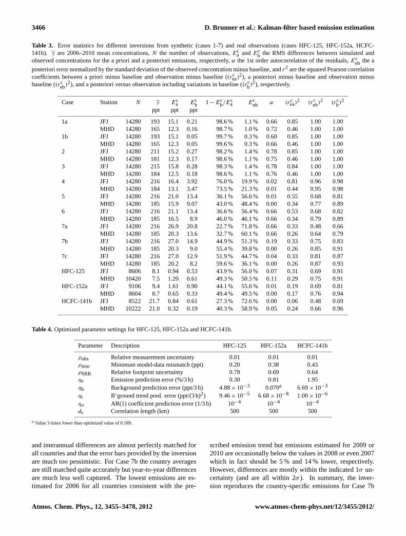
3466 D. Brunner et al.: Kalman-filter based emission estimation
Table 3. Error statistics for different inversions from synthetic (cases 1-7) and real observations (cases HFC-125, HFC-152a, HCFC-141b). y are 2006–2010 mean concentrations,N the number of observations,Ec
a andEcb the RMS differences between simulated and
observed concentrations for the a priori and a posteriori emissions, respectively,α the 1st order autocorrelation of the residuals,Ecnb the a
posteriori error normalized by the standard deviation of the observed concentration minus baseline, andr2 are the squared Pearson correlationcoefficients between a priori minus baseline and observation minus baseline ((rc
ea)2), a posteriori minus baseline and observation minus
baseline ((rceb)
2), and a posteriori versus observation including variations in baseline ((rcb)2), respectively.
Case Station N y Eca Ec
b 1− Ecb/Ec
a Ecnb α (rc
ea)2 (rc
eb)2 (rc
b)2
ppt ppt ppt
1a JFJ 14280 193 15.1 0.21 98.6 % 1.1 % 0.66 0.85 1.00 1.00MHD 14280 165 12.3 0.16 98.7 % 1.0 % 0.72 0.46 1.00 1.00
1b JFJ 14280 193 15.1 0.05 99.7 % 0.3 % 0.60 0.85 1.00 1.00MHD 14280 165 12.3 0.05 99.6 % 0.3 % 0.66 0.46 1.00 1.00
2 JFJ 14280 211 15.2 0.27 98.2 % 1.4 % 0.78 0.85 1.00 1.00MHD 14280 181 12.3 0.17 98.6 % 1.1 % 0.75 0.46 1.00 1.00
3 JFJ 14280 215 15.8 0.28 98.3 % 1.4 % 0.78 0.84 1.00 1.00MHD 14280 184 12.5 0.18 98.6 % 1.1 % 0.76 0.46 1.00 1.00
4 JFJ 14280 216 16.4 3.92 76.0 % 19.9 % 0.02 0.81 0.96 0.98MHD 14280 184 13.1 3.47 73.5 % 21.3 % 0.01 0.44 0.95 0.98
5 JFJ 14280 216 21.0 13.4 36.1 % 56.6 % 0.01 0.55 0.68 0.81MHD 14280 185 15.9 9.07 43.0 % 48.4 % 0.00 0.34 0.77 0.89
6 JFJ 14280 216 21.1 13.4 36.6 % 56.4 % 0.66 0.53 0.68 0.82MHD 14280 185 16.5 8.9 46.0 % 46.1 % 0.66 0.34 0.79 0.89
7a JFJ 14280 216 26.9 20.8 22.7 % 71.8 % 0.66 0.33 0.48 0.66MHD 14280 185 20.3 13.6 32.7 % 60.1 % 0.66 0.26 0.64 0.79
7b JFJ 14280 216 27.0 14.9 44.9 % 51.3 % 0.19 0.33 0.75 0.83MHD 14280 185 20.3 9.0 55.4 % 39.8 % 0.00 0.26 0.85 0.91
7c JFJ 14280 216 27.0 12.9 51.9 % 44.7 % 0.04 0.33 0.81 0.87MHD 14280 185 20.2 8.2 59.6 % 36.1 % 0.00 0.26 0.87 0.93
HFC-125 JFJ 8606 8.1 0.94 0.53 43.9 % 56.0 % 0.07 0.31 0.69 0.91MHD 10420 7.5 1.20 0.61 49.3 % 50.5 % 0.11 0.29 0.75 0.91
HFC-152a JFJ 9106 9.4 1.61 0.90 44.1 % 55.6 % 0.01 0.19 0.69 0.81MHD 8604 8.7 0.65 0.33 49.4 % 49.5 % 0.00 0.17 0.76 0.94
HCFC-141b JFJ 8522 21.7 0.84 0.61 27.3 % 72.6 % 0.00 0.06 0.48 0.69MHD 10222 21.0 0.32 0.19 40.3 % 58.9 % 0.05 0.24 0.66 0.96
Table 4. Optimized parameter settings for HFC-125, HFC-152a and HCFC-141b.
Parameter Description HFC-125 HFC-152a HCFC-141b
ρobs Relative measurement uncertainty 0.01 0.01 0.01ρmin Minimum model-data mismatch (ppt) 0.20 0.38 0.43ρSRR Relative footprint uncertainty 0.78 0.69 0.64ηe Emission prediction error (%/3 h) 0.30 0.81 1.95ηb Background prediction error (ppt/3 h) 4.88× 10⁻³ 0.070a 6.69× 10⁻³
ηt B’ground trend pred. error (ppt/(3 h)2) 9.46× 10⁻⁵ 6.68× 10⁻⁸ 1.00× 10⁻⁶
ηa AR(1) coefficient prediction error (1/3 h) 10−4 10−4 10−4
ds Correlation length (km) 500 500 500
a Value 3 times lower than optimized value of 0.189.
and interannual differences are almost perfectly matched forall countries and that the error bars provided by the inversionare much too pessimistic. For Case 7b the country averagesare still matched quite accurately but year-to-year differencesare much less well captured. The lowest emissions are es-timated for 2006 for all countries consistent with the pre-
scribed emission trend but emissions estimated for 2009 or2010 are occasionally below the values in 2008 or even 2007which in fact should be 5 % and 14 % lower, respectively.However, differences are mostly within the indicated 1σ un-certainty (and are all within 2σ ). In summary, the inver-sion reproduces the country-specific emissions for Case 7b
Atmos. Chem. Phys., 12, 3455–3478, 2012 www.atmos-chem-phys.net/12/3455/2012/

D. Brunner et al.: Kalman-filter based emission estimation 3467
D. Brunner et al.: Kalman-filter based emission estimation 25
(a) (b)
(c) (d)
Fig. 7. Emission inversion results for noise-free Case 3 (upper pan-els (a) and (b)) and noisy Case 7b (lower panels (c) and (d)). Pan-els (a) and (c) represent annual mean emissions (2006–2010) esti-mated for selected countries. Blue bars are country-mean a posteri-ori emissions estimated by the Kalman filter together with their 1σuncertainties. True reference emissions are overlaid as orange hori-zontal bars. Panels (b) and (d) are annual mean emission maps forthe year 2010.
Fig. 7. Emission inversion results for noise-free Case 3 (upper panels(a) and(b)) and noisy Case 7b (lower panels(c) and(d)). Panels(a)and(c) represent annual mean emissions (2006–2010) estimated for selected countries. Blue bars are country-mean a posteriori emissionsestimated by the Kalman filter together with their 1σ uncertainties. True reference emissions are overlaid as orange horizontal bars. Panels(b) and(d) are annual mean emission maps for the year 2010.
to within about 15–20 % and interannual differences largerthan this can be reproduced successfully.
4 European emissions of HFC-125, HFC-152a andHCFC-141b
This section presents the results of the inversion methodapplied to real observations of three different halocarbonsmeasured at Jungfraujoch and Mace Head, an analysis ofthe sensitivity of the results to different inversion settings,and a comparison with results obtained with the establishedmethod ofStohl et al.(2009).
In order to demonstrate the effect of the three iterationsapplied (see also Sect.2.4) on the estimated uncertainties,
Fig. 8 shows the evolution of the mean relative uncertaintyof the HFC-125 emissions. The simulation starts with a uni-form a-priori uncertainty of 200 %. After the first iteration,i.e. after assimilating the observations of the period 2006–2010 for the first time, the average uncertainty is reduced toabout 62 %. During the second iteration it is slightly reducedfurther to 58 % but remains constant thereafter, indicatingthat the uncertainty has essentially reached an equilibriumlevel already after the first iteration. Using the same obser-vations repeatedly does thus not lead to unrealistically lowuncertainties because in equilibrium the error reduction dueto the assimilation step (Eq.12) is exactly compensated bythe error increase due to the state prediction (Eq.5).
www.atmos-chem-phys.net/12/3455/2012/ Atmos. Chem. Phys., 12, 3455–3478, 2012

3468 D. Brunner et al.: Kalman-filter based emission estimation
26 D. Brunner et al.: Kalman-filter based emission estimation
Fig. 8. Evolution of the grid average relative uncertainty of HFC-125 emissions for the reference simulation during the three iterationsteps. The average uncertainty is calculated as
√trace(Pk)/Ne.
The x-axis is the number of 3-hr assimilation intervals and coversthe full period 2006-2010.
Fig. 8. Evolution of the grid average relative uncertainty of HFC-125 emissions for the reference simulation during the three iterationsteps. The average uncertainty is calculated as
√trace(Pk)/N
e. Thex-axis is the number of 3-h assimilation intervals and covers the fullperiod 2006–2010.
As an example for the quality of the simulations, Fig.9compares the observed time series of HFC-125 at Jungfrau-joch and Mace Head (black lines) with the correspondingtime series simulated by the Kalman filter (red). The darkblue line is the smooth background determined by the fil-ter. The right-hand panels further illustrate the excellentagreement by zooming into a selected period (1 November2009–15 February 2010). Note that despite the positive-definiteness of the estimated emissions, the red line can ex-tend below the background, which is a result of the AR(1)term in Eq. (13). Without considering this term, the cor-relation between observed and simulated time series (w/obackground) is lower,r = 0.65 instead of 0.83 at JFJ, andr = 0.75 instead of 0.87 at MHD. When including both theAR(1) term and the background concentrations, the correla-tions between simulated and measured concentrations (r withbgnd) are increased to 0.95 for both Jungfraujoch and MaceHead since a considerable fraction of the observed varianceis due to the long-term increase which can easily be tracedby the inversion.
Figure10 presents maps of 2009 annual mean emissions(average of all fields estimated for time steps between Jan-uary 2009 and December 2009 in units of kg km−2 yr−1)and corresponding 1σ uncertainties. These results were ob-tained with the parameter settings listed in Table4 obtainedwith the optimization procedure described in Sect.2.5. Thethree species show distinctly different spatial distributions.Emissions of HFC-125 are rather uniformly distributed overEurope with local hot spots in Italy, Germany, the Beneluxcountries and UK. Emissions in Eastern Europe are com-paratively low, particularly in the southeastern domain. Ex-pectedly low emissions over the Atlantic are successfully re-produced and the shape of the coastlines is well followed.
Uncertainties are lower than the estimated emissions in highemission areas but often in the range of the means in lowemission regions. Note that due to the estimation of the loga-rithm of emissions the model calculates relative (multiplica-tive) rather than absolute uncertainties. These were here sim-ply converted to absolute uncertainties by multiplication withthe mean. For an emission of 10 kg km−2 yr−1, for example,an uncertainty of 100 % in fact would mean that the emis-sions could be twice as high (i.e. 20 kg km−2 yr−1) or twiceas low (i.e. 5 kg km−2 yr−1) but not zero. Absolute uncer-tainties are thus not symmetric about the mean.
In comparison to HFC-125, HFC-152a emissions are quitelow in Germany and very low in Spain, Portugal, UK andIreland. Highest emissions are clearly identified in North-ern Italy but also the Benelux countries and France showsignificant emission levels. Finally, HCFC-141b, which iscontrolled by the Montreal Protocol and exhibits stronglydecreasing emissions in Europe since about 2003 (Derwentet al., 2007), shows pronounced hot spots in Italy and inFrance whereas emissions in most other countries are low(note the different color scale used for HCFC-141b). Franceis known to have been the main producing country of HCFC-141b in Europe. The large emissions from France are likelyrelated to HCFC-141b release from these production plantsfor which a-priori emissions were not available. Emissionuncertainties for HFC-141b are much larger than for theother two species often exceeding 100 %.
The improved agreement between simulated and measuredconcentrations achieved by the inversion is documented inthe lower part of Table3. RMS differences are reduced by27–49 % as compared to the a priori time series and correla-tions are strongly enhanced. The best performance was ob-tained for HFC-125 and HFC-152a while the concentrationsof HCFC-141b were more difficult to reproduce.
A problem specific to HFC-152a was the fact that the log-likelihood optimization assigned a large uncertainty to itsbackground concentrations with the consequence that the as-similation more willingly adjusted the background than theemissions. This lead to a highly variable background closelytracking the observations whereas the emission signals andhence the estimated emissions remained small, probably toosmall. Figure1b shows that for HFC-152a the baseline is infact quite variable and, different from the other two species,exhibits a pronounced seasonal cycle. The measurementsat Jungfraujoch exhibit many negative excursions below thebaseline (and below Mace Head background levels) whichare not instrumental artifacts but reflect true variability. Apreliminary analysis indicates that these “depletion events”are associated with advection from low latitudes (particularlyat Mace Head), and from the upper troposphere or strato-sphere (particularly at Jungfraujoch). HFC-152a has a strongnorth-south gradient due to its comparatively short lifetime(∼1.5 yr) and dominant sources in the Northern Hemisphereand probably has significant vertical gradients. Air massesoriginating from low latitudes are therefore associated with
Atmos. Chem. Phys., 12, 3455–3478, 2012 www.atmos-chem-phys.net/12/3455/2012/

D. Brunner et al.: Kalman-filter based emission estimation 3469
D. Brunner et al.: Kalman-filter based emission estimation 27
(a) (b)
(c) (d)
Fig. 9. Comparison of observed (black) and simulated (red) timeseries at (a),(b) Jungfraujoch and (c),(d) Mace Head from 2006 to2010. Dark blue lines are smooth backgrounds estimated by theKalman filter. The panels to the right present a zoom on the period1 Nov 2009 - 15 Feb 2010.
Fig. 9. Comparison of observed (black) and simulated (red) time series at(a),(b) Jungfraujoch and(c),(d) Mace Head from 2006 to 2010.Dark blue lines are smooth backgrounds estimated by the Kalman filter. The panels to the right present a zoom on the period 1 November2009–15 February 2010.
lower background values than air masses from high latitudes.The inversion tries to reproduce this variability by assign-ing a large uncertainty to the background. In future inver-sions of HFC-152a it would therefore be desirable to explic-itly account for the influence of advection from different re-gions on background fluctuations. As a preliminary solutionwe reduced the background uncertainty by a factor of threewhich leads to a smoother background and in turn to higheremissions: European emissions are on average enhanced byabout 20 % suggesting that the treatment of the backgroundvariability represents a major uncertainty in our HFC-152aemission estimates.
The evolution of country-averaged emissions of HFC-125,HFC-152a and HCFC-141b over the five years 2006–2010is displayed in Fig.11. Red columns correspond to emis-sions in 2009 reported to UNFCCC (2011 downloads, avail-able only for HFC-125 and HFC-152a), which can be com-pared with the second to last column in each group of bluecolumns representing our estimates. Orange bars are emis-sions reported for the year 2006. A quantitative summary ofall values for the years 2006 and 2009 is provided in Table5.
For Germany, France, the UK and the Benelux countriesour estimates for HFC-125 are close (within 21 %) to the val-ues reported to UNFCCC for both 2006 and 2009. All coun-
tries except Ireland reported increasing emissions of HFC-125 between 2006 and 2009 which agrees well with the esti-mated changes. Italy reports a very large increase by 42 %from 2006 to 2009 which is larger than our estimated in-crease of 24±19 %. Reported (estimated) changes for Ger-many, France, UK and Benelux are 9 % (16±19 %), 26 %(11±13 %), 10 % (9±13 %), and 29 % (5±22 %) suggestingthat increases in Italy, France and Benelux were somewhatsmaller than reported. However, given the large uncertain-ties in the annual values these differences are only marginallysignificant. Overall, the reported and estimated changes arein reasonable agreement.
Larger discrepancies between reported and estimatedemissions are obtained for Italy, Switzerland, Ireland,Spain+ Portugal, and Austria. Despite its vicinity toJungfraujoch, an accurate assessment of Swiss emissions isdifficult due to the small area of the country. In addition,the transport model used is scarcely sufficient to resolvethe processes responsible for uplift of air from the SwissPlateau to Jungfraujoch which is often associated with com-plex thermally-induced wind systems and convective bound-ary layers over the Alpine topography. Similar argumentsalso hold for Austria. The large discrepancy for Ireland with187 % to 312 % higher emissions obtained by the inversion,
www.atmos-chem-phys.net/12/3455/2012/ Atmos. Chem. Phys., 12, 3455–3478, 2012

3470 D. Brunner et al.: Kalman-filter based emission estimation
28 D. Brunner et al.: Kalman-filter based emission estimation
(a) HFC-125 a posteriori emissions (b) HFC-125 uncertainty
(c) HFC-152a a posteriori emissions (d) HFC-152a uncertainty
(e) HCFC-141b a posteriori emissions (f) HCFC-141b uncertainty
Fig. 10. Distribution of annual mean emissions (left) and their un-certainties (right) of HFC-125, HFC-152a and HCFC-141 in Europein 2009.
Fig. 10. Distribution of annual mean emissions (left) and their uncertainties (right) of HFC-125, HFC-152a and HCFC-141 in Europe in2009.
on the other hand, is surprising. Our estimates are in goodagreement with a recent British study which also estimatedmuch larger than reported HFC-125 emissions from Irelandof 69 Mg yr−1 in 2006 and 80 Mg yr−1 in 2009, respectively(O’Doherty et al., 2011).
Figure1a displays several large HFC-125 peaks which arelikely due to the effect of nearby emissions in conjunctionwith low-wind speeds. Situations with low-winds and lowboundary layer heights with correspondingly large sensitivi-
ties for local emissions were therefore filtered out in the in-version studies ofManning et al.(2003) andManning et al.(2011). Excluding these peaks, however, has a negligible im-pact on our results (e.g. reducing the 2009 value from 84 to83 Mg yr−1) suggesting that local effects are insufficient toexplain the discrepancy. A large and significant discrepancyalso exists for Spain+ Portugal with estimated emissions be-ing 150–170 % higher than the reported numbers. However,these results should be considered with care since the two
Atmos. Chem. Phys., 12, 3455–3478, 2012 www.atmos-chem-phys.net/12/3455/2012/

D. Brunner et al.: Kalman-filter based emission estimation 3471
Table 5. Estimated country-specific emissions of HFC-125, HFC-152a and HCFC-141b. For HFC-125 and HFC-152a the UNFCCC bottom-up values are also provided for comparison. Although the inversion provides relative uncertainties due to the estimation of the logarithm ofemissions, uncertainties are indicated as absolute errors (1σ ) by multiplying the estimated emission by its relative uncertainty. For the totalof all 12 countries the uncertainty was estimated as the mean squared error.
Country Year HFC-125 HFC-152a HCFC-141ba posteriori UNFCCC diff. a posteriori UNFCCC diff. a posteriori(Mg yr−1) (Mg yr−1) (%) (Mg yr−1) (Mg yr−1) (%) (Mg yr−1)
Switzerland 2006 11 ±2 63 −81.5 9 ±2 15 −38.7 21 ±6Switzerland 2009 13 ±2 75 −82.0 6 ±1 1 482.6 11 ±4Germany 2006 589 ±69 594 −0.8 457 ±82 449 1.9 200 ±82Germany 2009 683 ±80 647 5.6 351 ±62 782 −55.0 119 ±47Italy 2006 936 ±100 691 35.5 729 ±139 NA NA 451 ±170Italy 2009 1158 ±128 983 17.8 803 ±135 NA NA 269 ±116France 2006 731 ±61 814 −10.3 331 ±45 313 5.8 768 ±257France 2009 812 ±67 1032 −21.3 324 ±47 388 −16.5 276 ±67Spain+Portugal 2006 689 ±88 252 173.1 225 ±71 413 −45.5 238 ±114Spain+Portugal 2009 861 ±111 341 152.0 171 ±63 354 −51.6 208 ±101United Kingdom 2006 611 ±53 710 −13.8 59 ±14 166 −64.0 131 ±40United Kingdom 2009 665 ±57 783 −15.1 68 ±16 114 −40.4 108 ±33Ireland 2006 78 ±7 27 187.4 12 ±2 6 84.3 23 ±6Ireland 2009 84 ±7 20 312.1 13 ±2 7 80.6 20 ±5Benelux 2006 223 ±33 219 2.1 80 ±16 211 −61.8 41 ±20Benelux 2009 235 ±34 283 −17.0 90 ±18 349 −74.1 43 ±22Austria 2006 32 ±10 67 −51.9 57 ±20 249 −76.9 44 ±36Austria 2009 39 ±12 79 −50.5 59 ±23 130 −54.1 18 ±12Total 12 countries 2006 3905 ±174 3412 14.4 1965 ±185 1818 8.1 1919 ±344Total 12 countries 2009 4555 ±210 4227 7.8 1889 ±172 2121 −10.9 1077 ±180
observation sites are only weakly sensitive to emissions fromSpain and Portugal.
Total emissions summed over the 12 countries are only 8-14 % higher than the UNFCCC bottom-up estimates. Thetotal of 3905 Mg yr−1 for the year 2006 agrees very favor-ably with the 3800 Mg yr−1 and 4700 Mg yr−1 estimated byO’Doherty et al.(2009) for the EU-15 region using a COinterspecies correlation technique and the NAME model, re-spectively. The EU-15 region includes the same 12 coun-tries minus Switzerland plus Denmark, Sweden, Finland andGreece. Based on UNFCCC values, EU-15 emissions can beexpected to be higher than the total of our 12 countries byonly about 174 Mg yr−1.
Results for HFC-152a are less consistent with UNFCCCnumbers for individual countries both regarding the mag-nitude of emissions and their trends. Italy does not reportHFC-152a emissions to the UNFCCC. Our results, however,suggest Italy to have the largest emissions in the study area.Emissions reported by Germany very closely match our es-timate in 2006 but are much higher in 2009 due to oppos-ing trends. Spain+ Portugal report larger emissions of HFC-152a than of HFC-125 in strong contrast to our estimatessuggesting that HFC-152a emissions are about 3–5 timeslower than those of HFC-125. For UK our estimates are 40–60 % lower than the official numbers and while UK reportsa marked decrease from 2006 to 2009 our results suggest a
small increase. Emissions reported by France are broadlyconsistent with our estimates, whereas those reported by theBenelux countries are at least a factor of 2.6–3.9 higher thanour top-down values. The total over all 12 countries is con-sistent with the bottom-up estimates with 8 % higher valuesthan UNFCCC in 2006 and 11 % lower values in 2009 sug-gesting that non-reported emissions from Italy are to someextent absorbed by other countries. The total emission of1965 Mg yr−1 in 2006 is well in the range of total Europeanemissions of 1500–4000 Mg yr−1 estimated byGreally et al.(2007) for the year 2004.
The results for HCFC-141b indicate an ongoing decreasein almost all countries continuing the negative trend ob-served since about 2002 (Derwent et al., 2007). Differentfrom the two other species, the largest emissions are obtainedfor France, though these emissions dramatically dropped be-tween 2007 and 2009 by more than a factor of two. A de-crease by more than a factor of two is also found for Italythough spread more uniformly over the five years. Totalemissions of the 12 countries were almost cut in half be-tween 2006 and 2009 from 1919 Mg yr−1 to 1077 Mg yr−1
which is broadly in line with total European emissions of3100–4900 Mg yr−1 estimated for the year 2004 using a COinterspecies correlation method or the 5500–6100 Mg yr−1
obtained using the NAME model (Derwent et al., 2007).
www.atmos-chem-phys.net/12/3455/2012/ Atmos. Chem. Phys., 12, 3455–3478, 2012
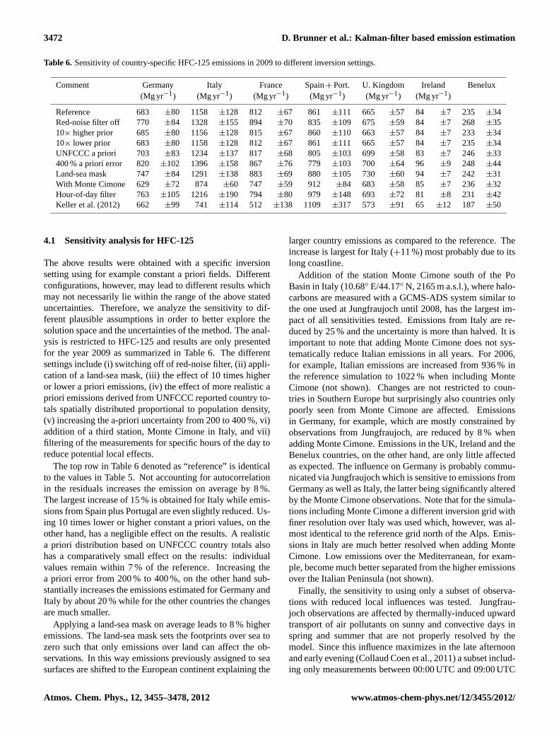
3472 D. Brunner et al.: Kalman-filter based emission estimation
Table 6. Sensitivity of country-specific HFC-125 emissions in 2009 to different inversion settings.
Comment Germany Italy France Spain+ Port. U. Kingdom Ireland Benelux(Mg yr−1) (Mg yr−1) (Mg yr−1) (Mg yr−1) (Mg yr−1) (Mg yr−1)
Reference 683 ±80 1158 ±128 812 ±67 861 ±111 665 ±57 84 ±7 235 ±34Red-noise filter off 770 ±84 1328 ±155 894 ±70 835 ±109 675 ±59 84 ±7 268 ±3510× higher prior 685 ±80 1156 ±128 815 ±67 860 ±110 663 ±57 84 ±7 233 ±3410× lower prior 683 ±80 1158 ±128 812 ±67 861 ±111 665 ±57 84 ±7 235 ±34UNFCCC a priori 703 ±83 1234 ±137 817 ±68 805 ±103 699 ±58 83 ±7 246 ±33400 % a priori error 820 ±102 1396 ±158 867 ±76 779 ±103 700 ±64 96 ±9 248 ±44Land-sea mask 747 ±84 1291 ±138 883 ±69 880 ±105 730 ±60 94 ±7 242 ±31With Monte Cimone 629 ±72 874 ±60 747 ±59 912 ±84 683 ±58 85 ±7 236 ±32Hour-of-day filter 763 ±105 1216 ±190 794 ±80 979 ±148 693 ±72 81 ±8 231 ±42Keller et al.(2012) 662 ±99 741 ±114 512 ±138 1109 ±317 573 ±91 65 ±12 187 ±50
4.1 Sensitivity analysis for HFC-125
The above results were obtained with a specific inversionsetting using for example constant a priori fields. Differentconfigurations, however, may lead to different results whichmay not necessarily lie within the range of the above stateduncertainties. Therefore, we analyze the sensitivity to dif-ferent plausible assumptions in order to better explore thesolution space and the uncertainties of the method. The anal-ysis is restricted to HFC-125 and results are only presentedfor the year 2009 as summarized in Table6. The differentsettings include (i) switching off of red-noise filter, (ii) appli-cation of a land-sea mask, (iii) the effect of 10 times higheror lower a priori emissions, (iv) the effect of more realistic apriori emissions derived from UNFCCC reported country to-tals spatially distributed proportional to population density,(v) increasing the a-priori uncertainty from 200 to 400 %, vi)addition of a third station, Monte Cimone in Italy, and vii)filtering of the measurements for specific hours of the day toreduce potential local effects.
The top row in Table6 denoted as “reference” is identicalto the values in Table5. Not accounting for autocorrelationin the residuals increases the emission on average by 8 %.The largest increase of 15 % is obtained for Italy while emis-sions from Spain plus Portugal are even slightly reduced. Us-ing 10 times lower or higher constant a priori values, on theother hand, has a negligible effect on the results. A realistica priori distribution based on UNFCCC country totals alsohas a comparatively small effect on the results: individualvalues remain within 7 % of the reference. Increasing thea priori error from 200 % to 400 %, on the other hand sub-stantially increases the emissions estimated for Germany andItaly by about 20 % while for the other countries the changesare much smaller.
Applying a land-sea mask on average leads to 8 % higheremissions. The land-sea mask sets the footprints over sea tozero such that only emissions over land can affect the ob-servations. In this way emissions previously assigned to seasurfaces are shifted to the European continent explaining the
larger country emissions as compared to the reference. Theincrease is largest for Italy (+11 %) most probably due to itslong coastline.
Addition of the station Monte Cimone south of the PoBasin in Italy (10.68◦ E/44.17◦ N, 2165 m a.s.l.), where halo-carbons are measured with a GCMS-ADS system similar tothe one used at Jungfraujoch until 2008, has the largest im-pact of all sensitivities tested. Emissions from Italy are re-duced by 25 % and the uncertainty is more than halved. It isimportant to note that adding Monte Cimone does not sys-tematically reduce Italian emissions in all years. For 2006,for example, Italian emissions are increased from 936 % inthe reference simulation to 1022 % when including MonteCimone (not shown). Changes are not restricted to coun-tries in Southern Europe but surprisingly also countries onlypoorly seen from Monte Cimone are affected. Emissionsin Germany, for example, which are mostly constrained byobservations from Jungfraujoch, are reduced by 8 % whenadding Monte Cimone. Emissions in the UK, Ireland and theBenelux countries, on the other hand, are only little affectedas expected. The influence on Germany is probably commu-nicated via Jungfraujoch which is sensitive to emissions fromGermany as well as Italy, the latter being significantly alteredby the Monte Cimone observations. Note that for the simula-tions including Monte Cimone a different inversion grid withfiner resolution over Italy was used which, however, was al-most identical to the reference grid north of the Alps. Emis-sions in Italy are much better resolved when adding MonteCimone. Low emissions over the Mediterranean, for exam-ple, become much better separated from the higher emissionsover the Italian Peninsula (not shown).
Finally, the sensitivity to using only a subset of observa-tions with reduced local influences was tested. Jungfrau-joch observations are affected by thermally-induced upwardtransport of air pollutants on sunny and convective days inspring and summer that are not properly resolved by themodel. Since this influence maximizes in the late afternoonand early evening (Collaud Coen et al., 2011) a subset includ-ing only measurements between 00:00 UTC and 09:00 UTC
Atmos. Chem. Phys., 12, 3455–3478, 2012 www.atmos-chem-phys.net/12/3455/2012/
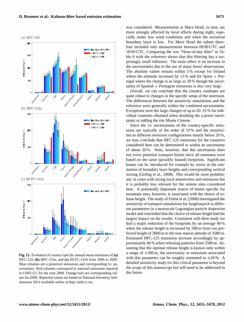
D. Brunner et al.: Kalman-filter based emission estimation 3473
D. Brunner et al.: Kalman-filter based emission estimation 29
(a) HFC-125
(b) HFC-152a
(c) HCFC-141b
Fig. 11. Evolution of country-specific annual mean emissions of (a)HFC-125, (b) HFC-152a, and (c) HCFC-141b from 2006 to 2009.Blue columns are a posteriori emissions and corresponding 1σ un-certainties. Red columns correspond to national emissions reportedto UNFCCC for the year 2009. Orange bars are corresponding val-ues for 2006. Reported values are based on National Inventory Sub-missions 2011 available online at http://unfccc.int.
Fig. 11.Evolution of country-specific annual mean emissions of(a)HFC-125,(b) HFC-152a, and(c) HCFC-141b from 2006 to 2009.Blue columns are a posteriori emissions and corresponding 1σ un-certainties. Red columns correspond to national emissions reportedto UNFCCC for the year 2009. Orange bars are corresponding val-ues for 2006. Reported values are based on National Inventory Sub-missions 2011 available online athttp://unfccc.int.
was considered. Measurements at Mace Head, in turn, aremore strongly affected by local effects during night, espe-cially under low wind conditions and when the nocturnalboundary layer is low. For Mace Head the subset there-fore included only measurements between 09:00 UTC and18:00 UTC. Comparing the row “Hour-of-day filter” in Ta-ble 6 with the reference shows that this filtering has a sur-prisingly small influence. The main effect is an increase inthe uncertainties due to the use of many fewer observations.The absolute values remain within 5 % except for Irelandwhere the estimate increases by 13 % and for Spain+ Por-tugal where the change is as large as 39 % though the uncer-tainty of Spanish+ Portugese emissions is also very large.
Overall, we can conclude that the country estimates arequite robust to changes in the specific setup of the inversion.The differences between the sensitivity simulations and thereference were generally within the combined uncertainties.Exceptions were the large changes of up to 20–25 % for indi-vidual countries obtained when doubling the a-priori uncer-tainty or adding the site Monte Cimone.
Since the 1σ uncertainties of the country-specific emis-sions are typically of the order of 10 % and the sensitivi-ties to different inversion configurations mostly below 20 %,we may conclude that HFC-125 emissions for the countriesconsidered here can be determined to within an uncertaintyof about 20 %. Note, however, that this uncertainty doesnot cover potential transport biases since all estimates werebased on the same (possibly biased) footprints. Significantbiases can be introduced for example by errors in the esti-mation of boundary layer heights and corresponding verticalmixing (Gerbig et al., 2008). This would be most problem-atic in cases with strong local sensitivities and emissions butit is probably less relevant for the remote sites consideredhere. A potentially important source of biases specific formountain sites, however, is associated with the choice of re-lease height. The study ofFolini et al.(2008) investigated thesensitivity of transport simulations for Jungfraujoch to differ-ent parameters in a mesoscale Lagrangian particle dispersionmodel and concluded that the choice of release height had thelargest impact on the results. Consistent with their study wefind a major reduction of the footprints by on average 40 %when the release height is increased by 580 m from our pre-ferred height of 3000 m to the true station altitude of 3580 m.Estimated HFC-125 emissions increase accordingly by ap-proximately 40 % when releasing particles from 3580 m. As-suming that the optimal release height is known only withina range of±300 m, the uncertainty in emissions associatedwith this parameter can be roughly estimated to±20 %. Adetailed sensitivity study for this critical parameter is beyondthe scope of this manuscript but will need to be addressed inthe future.
www.atmos-chem-phys.net/12/3455/2012/ Atmos. Chem. Phys., 12, 3455–3478, 2012

3474 D. Brunner et al.: Kalman-filter based emission estimation
4.2 Comparison with Bayesian inversion
The last row in Table6 presents country emissions estimatedby Keller et al.(2012) using a Bayesian approach similar tothe method ofStohl et al.(2009), and using the same FLEX-PART model output as used here. Since their study includedthe measurements from Monte Cimone and the Eastern Eu-ropean site K-Puszta, the numbers may be best comparedwith the row labeled “With Monte Cimone”. Uncertaintiesreported byKeller et al. (2012) were derived as a maxi-mum of an analytical uncertainty and an uncertainty derivedfrom sensitivity runs and therefore tend to be larger thanour estimates. For most countries except Spain+ Portugaland Germany the estimates byKeller et al.(2012) are some-what lower. Emissions from Germany and Italy agree within8 %. Emissions from UK, Ireland, and the Benelux countriesare 16 %, 24 % and 21 % lower than our numbers, respec-tively, but these differences are within the combined uncer-tainties and thus not significant.Keller et al. (2012) esti-mated 22 % higher emissions from Spain+ Portugal but theyalso assigned a large uncertainty to their estimate coveringour value. The only significant difference is obtained forFrance where the estimate ofKeller et al. (2012) is 31 %lower than ours. The reason for this discrepancy is presentlynot known and will require further investigation. Note thatour estimate for France is still 19 % below UNFCCC. Our es-timates also compare favorably withO’Doherty et al.(2011)for Ireland (85±7 Mg yr−1 versus 80±30 Mg yr−1) and theUK (683±58 Mg yr−1 versus 730±170 Mg yr−1). For the re-gion denoted NW EU (= UK, IRL, BENELUX, GER, FRA,DEN) in O’Doherty et al.(2011) our estimate of 2380 Mg t−1
is in between the 3300 Mg yr−1 estimated in that study andthe value of 2072 Mg t−1 reported byKeller et al.(2012).
5 Conclusions
An inversion method based on an extended Kalman filter wasdeveloped to estimate regional scale emissions and their in-terannual changes of passive or weakly reactive trace gaseswith positive fluxes from the surface to the atmosphere. Forgases like CO2, which do not only have large emission fluxesbut also significant uptake at the surface, the method wouldhave to be modified to incorporate negative fluxes and to ac-count for potentially strong temporal variability of surfacefluxes. The particular features of the presented method in-clude positive-definiteness of the emissions, the inclusion ofmeasurement-site-specific background concentrations in thestate vector to estimate a smoothly varying background perstation along with the emission field, and the considerationof temporal correlations in the residuals by applying an aug-mented state red-noise Kalman filter. The dynamic model de-scribing the evolution of the state vector from one time stepto the next assumes persistence of the emissions and allowsfor a linearly changing background. The covariance matrices
describing the model-data mismatch (due to both measure-ment and transport model errors) and the uncertainty of thestate projection are described by a few parameters objectivelydetermined by log-likelihood maximization. A realistic de-scription of these errors is crucial for optimal results and re-liable a posteriori uncertainties.
The application of a Kalman filter, which adjusts the emis-sion field through sequential assimilation of observationsrather than solving the problem for all observations of a givenperiod at once as done in “batch inversions” (Bruhwiler et al.,2005), allows solving comparatively large inversion prob-lems using conventional computational resources. The com-putationally limiting part will in most cases be the calculationof the source-receptor-relationships (SRR) with a transportmodel, not the inversion.
Irrespective of the mathematical details of the methodused, the quality of the transport model is a key factor in anyinversion study, in particular when addressing regional scaleemissions. In our case we employed the Lagrangian parti-cle dispersion model FLEXPART in backward mode drivenby ECMWF meteorology at a relatively high resolution ofabout 20× 20 km2 beneficial for simulating transport to sta-tions in a complex environment such as the high alpine siteJungfraujoch.
The inversion method was demonstrated for a series of ide-alized simulations with synthetic data as well as for estimat-ing emissions of HFC-125, HFC-152a and HCFC-141b inEurope using real observations from Jungfraujoch, Switzer-land, and Mace Head, Ireland. For noise-free synthetic ob-servations the solution converged towards the reference fieldused for generating the synthetic data confirming the cor-rect setup. With increased levels of noise assigned to thesynthetic time series the solutions increasingly differed fromthe true emissions and these differences were shown to belarger when error covariances did not reflect true uncertain-ties. Accounting for correlated residuals by applying a red-noise Kalman filter clearly improved the agreement with thereference emissions. Seasonal variations and trends imposedon the synthetic backgrounds were successfully traced by theinverted background concentrations and had only little im-pact on the quality of the emission estimates. Based on sim-ulations with synthetic time series with similar properties asreal observations we conclude that differences in country-specific annual mean emissions need to be larger than about15–20 % between two different years to be detectable basedon observations from Jungfraujoch and Mace Head only.
Estimated emissions of HFC-125 were mostly consistentwith bottom-up values as reported to UNFCCC in the frame-work of the Kyoto Protocol. Both the reported numbers andthe inversion showed increasing emissions between 2006 to2010. Emissions reported by Ireland were significantly lowerby a factor of 2–3 with an increasing discrepancy during thelatest years. Results for HFC-152a were much more scat-tered with estimated emissions being significantly lower thanreported for Germany, Spain+ Portugal, the UK and the
Atmos. Chem. Phys., 12, 3455–3478, 2012 www.atmos-chem-phys.net/12/3455/2012/

D. Brunner et al.: Kalman-filter based emission estimation 3475
Benelux countries, but higher for Ireland. Italy, which so fardoes not report HFC-152a emissions to UNFCCC, showedthe highest emissions of all countries considered. HCFC-141b showed strongly decreasing emissions in nearly allcountries as expected due to its regulation under the MontrealProtocol. Large emissions of the order of 800–1000 Mg yr−1
were estimated for France for the years 2006 and 2007 fol-lowed by a sharp decline in the following years. Emissionsfrom Switzerland and Austria seem not to be reliably cap-tured by the inversion probably due to difficulties in simulat-ing transport from the boundary layers of these countries tothe high Alpine site Jungfraujoch.
A posteriori 1σ uncertainties of country-specific annualemissions were typically in the range of 10–20 % for HFC-125, 15–30 % for HFC-152a and 20–40 % for HCFC-141b(Table5). A sensitivity analysis for HFC-125 indicated thatcountry-specific emissions vary by less than 25 % for differ-ent setups of the inversion including varying a-priori distri-butions and uncertainties, the application of a land-sea mask,and the addition of the station Monte Cimone in Italy. An ad-ditional uncertainty specific for HFC-152a is associated withthe simulation of its strongly variable background. Theseuncertainties do not yet account for potential biases in thetransport simulations which can be caused by several factors(Manning, 2011). A particularly relevant uncertainty specificfor mountain sites is the choice of particle release height. Wedetermined the optimal release height for Jungfraujoch to bearound 3000 m a.s.l. for the model configuration used, buthigher or lower release heights within the range of uncer-tainty would lead to up to 20 % higher or lower emissions,respectively.
Reported country emissions were often outside the uncer-tainty range of the a posteriori emissions. Together with thefact that for selected countries the agreement between esti-mated and reported values varies strongly between differentcompounds, this provides clear evidence for inconsistenciesin the bottom-up estimates that can be readily identified bytop-down methods.
The method presented here will be compared with othertop-down approaches in the framework of the EC FP7 projectINGOS. Such a multi-model approach is crucial to improveour understanding of model uncertainties and the ability toderive country-specific estimates. A robust quantification ofuncertainties is needed to further strengthen top-down meth-ods as complementary approach to the bottom-up emissionestimates (Nisbet and Weiss, 2010).
Acknowledgements.The measurements at Jungfraujoch are part ofthe Swiss National Air Pollution Monitoring Network (NABEL)and the HALCLIM-project and are supported by the SwissFederal Office for the Environment (FOEN). We also acknowledgethe International Foundation “High Altitude Research StationsJungfraujoch and Gornergrat” for providing an excellent infras-tructure. The operation of the Mace Head station was supportedby the Department of the Energy and Climate Change (DECC,UK) (contracts GA01081 and GA01103 to the University of
Bristol). The Swiss National Science Foundation is acknowledgedfor partly financing the IPAZIA computational cluster (project206021128754) on which FLEXPART calculations were per-formed.
Edited by: N. Harris
References
Baker, D. F., Law, R. M., Gurney, K. R., Rayner, P., Peylin, P.,Denning, A. S., Bousquet, P., Bruhwiler, L., Chen, Y. H.,Ciais, P., Fung, I. Y., Heimann, M., John, J., Maki, T., Maksyu-tov, S., Masarie, K., Prather, M., Pak, B., Taguchi, S., andZhu, Z.: TransCom 3 inversion intercomparison: impact oftransport model errors on the interannual variability of regionalCO2 fluxes, 1988–2003, Global Biogeochem. Cy., 20, GB1002,doi:10.1029/2004GB002439, 2006.
Bergamaschi, P., Krol, M., Dentener, F., Vermeulen, A., Mein-hardt, F., Graul, R., Ramonet, M., Peters, W., and Dlugo-kencky, E. J.: Inverse modelling of national and EuropeanCH4 emissions using the atmospheric zoom model TM5, At-mos. Chem. Phys., 5, 2431–2460,doi:10.5194/acp-5-2431-2005,2005.
Bousquet, P.: Methane sources and sinks of the past two decades:what did we learn with atmospheric inversions?, 19th AnnualVM Goldschmidt Conference, Davos, Switzerland, 21 June2009, Geochim. Cosmochim. Ac., 73, A149, 2009.
Bousquet, P., Ciais, P., Miller, J. B., Dlugokencky, E. J., Hauglus-taine, D. A., Prigent, C., Van der Werf, G. R., Peylin, P.,Brunke, E. G., Carouge, C., Langenfelds, R. L., Lathiere, J.,Papa, F., Ramonet, M., Schmidt, M., Steele, L. P., Tyler, S. C.,and White, J.: Contribution of anthropogenic and natural sourcesto atmospheric methane variability, Nature, 443, 439–443,doi:10.1038/nature05132, 2006.
Bruhwiler, L. M. P., Michalak, A. M., Peters, W., Baker, D. F., andTans, P.: An improved Kalman Smoother for atmospheric inver-sions, Atmos. Chem. Phys., 5, 2691–2702,doi:10.5194/acp-5-2691-2005, 2005.
Brunner, D., Staehelin, J., Kunsch, H. R., and Bodeker, G. E.:A Kalman filter reconstruction of the vertical ozone distribu-tion in an equivalent latitude – potential temperature frameworkfrom TOMS/GOME/SBUV total ozone observations, J. Geo-phys. Res., 111, D12308,doi:10.1029/2005JD006279, 2006.
Chen, Y.-H. and Prinn, R. G.: Estimation of atmospheric methaneemissions between 1996 and 2001 using a three-dimensionalglobal chemical transport model, J. Geophys. Res., 111, D10307,doi:10.1029/2005JD006058, 2006.
Collaud Coen, M., Weingartner, E., Furger, M., Nyeki, S.,Prevot, A. S. H., Steinbacher, M., and Baltensperger, U.: Aerosolclimatology and planetary boundary influence at the Jungfrau-joch analyzed by synoptic weather types, Atmos. Chem. Phys.,11, 5931–5944,doi:10.5194/acp-11-5931-2011, 2011.
Cunnold, D. M., Fraser, P. J., Weiss, R. F., Prinn, R. G., Sim-monds, P. G., Miller, B. R., Alyea, F. N., and Crawford, A. J.:Global trends and annual releases of CCl3F and CCl2F2 esti-mated from ALE/GAGE and other measurements from July 1978to June 1991, J. Geophys. Res., 99, 1107–1126, 1994.
Derwent, R. G., Simmonds, P. G., Greally, B. R., O’doherty, S.,McCulloch, A., Manning, A., Reimann, S., Folini, D., and
www.atmos-chem-phys.net/12/3455/2012/ Atmos. Chem. Phys., 12, 3455–3478, 2012

3476 D. Brunner et al.: Kalman-filter based emission estimation
Vollmer, M. K.: The phase-in and phase-out of European emis-sions of HCFC-141b and HCFC-142b under the Montreal Pro-tocol: evidence from observations at Mace Head, Ireland andJungfraujoch, Switzerland from 1994 to 2004, Atmos. Environ.,41, 757–767,doi:10.1016/j.atmosenv.2006.09.009, 2007.
Engelen, R. J., Denning, A. S., Gurney, K. R., Law, R. M.,Denning, A. S., Rayner, P. J., Baker, D., Bousquet, P., Bruh-wiler, L., Chen, Y. H., Ciais, P., Fan, S., Fung, I. Y., Gloor, M.,Heimann, M., Higuchi, K., John, J., Maki, T., Maksyutov, S.,Masarie, K., Peylin, P., Prather, M., Pak, B. C., Sarmiento, J.,Taguchi, S., Takahashi, T., and Yuen, C. W.: On error estimationin atmospheric CO2 inversions, J. Geophys. Res., 111, D14199,doi:10.1029/2006JD007428, 2006.
Folini, D., Ubl, S., and Kaufmann, P.: Lagrangian particle disper-sion modeling for the high Alpine site Jungfraujoch, J. Geophys.Res., 113, D18111,doi:10.1029/2007JD009558, 2008.
Gerbig, C., Korner, S., and Lin, J. C.: Vertical mixing in atmo-spheric tracer transport models: error characterization and prop-agation, Atmos. Chem. Phys., 8, 591–602,doi:10.5194/acp-8-591-2008, 2008.
Gockede, M., Michalak, A. M., Vickers, D., Turner, D. P., andLaw, B. E.: Atmospheric inverse modeling to constrain regional-scale CO2 budgets at high spatial and temporal resolution, J.Geophys. Res., 115, D15113,doi:10.1029/2009JD012257, 2010.
Greally, B. R., Manning, A. J., Reimann, S., McCulloch, A.,Huang, J., Dunse, B. L., Simmonds, P. G., Prinn, R. G.,Fraser, P. J., Cunnold, D. M., O’Doherty, S., Porter, L. W.,Stemmler, K., Vollmer, M. K., Lunder, C. R., Schmidbauer, N.,Hermansen, O., Arduini, J., Salameh, P. K., Krummel, P. B.,Wang, R. H. J., Folini, D., Weiss, R. F., Maione, M., Nick-less, G., Stordal, F., and Derwent, R. G.: Observations of1,1-difluoroethane (HFC-152a) at AGAGE and SOGE mon-itoring stations in 1994–2004 and derived global and re-gional emission estimates, J. Geophys. Res., 112, D06308,doi:10.1029/2006JD007527, 2007.
Gurney, K. R., Law, R. M., Denning, A. S., Rayner, P. J., Baker, D.,Bousquet, P., Bruhwiler, L., Chen, Y. H., Ciais, P., Fan, S.,Fung, I. Y., Gloor, M., Heimann, M., Higuchi, K., John, J.,Maki, T., Maksyutov, S., Masarie, K., Peylin, P., Prather, M.,Pak, B. C., Randerson, J., Sarmiento, J., Taguchi, S., Taka-hashi, T., and Yuen, C. W.: Towards robust regional estimatesof CO2 sources and sinks using atmospheric transport models,Nature, 415, 626–630, 2002.
Hartley, D. and Prinn, R.: Feasibility of determining surfaceemissions of trace gases using an inverse method in a three-dimensional chemical transport model, J. Geophys. Res., 98,5183–5197, 1993.
Harvey, A. C.: Forecasting, Structural Time Series Models and theKalman Filter, Cambridge University Press, New York, USA,1989.
Henne, S., Furger, M., and Prevot, A. S. H.: Climatology of moun-tain venting induced moisture layers in the lee of the Alps, J.Appl. Meteorol., 44, 620–633, 2005.
Henne, S., Brunner, D., Folini, D., Solberg, S., Klausen, J., andBuchmann, B.: Assessment of parameters describing representa-tiveness of air quality in-situ measurement sites, Atmos. Chem.Phys., 10, 3561–3581,doi:10.5194/acp-10-3561-2010, 2010.
Hirsch, A. I., Michalak, A. M., Bruhwiler, L. M., Peters, W., Dlugo-kencky, E. J., and Tans, P. P.: Inverse modeling estimates of the
global nitrous oxide surface flux from 1998–2001, Global Bio-geochem. Cy., 20, GB1008,doi:10.1029/2004GB002443, 2006.
Houweling, S., Kaminski, T., Dentener, F., Lelieveld, J., andHeimann, M.: Inverse modeling of methane sources and sinksusing the adjoint of a global transport model, J. Geophys. Res.,104, 26137–26160, 1999.
Kalman, R. H. and Bucy, R. S.: New results in linear filtering andprediction theory, J. Basic Eng., 83D, 95–108, 1961.
Kaminski, T., Rayner, P. J., Heimann, M., and Enting, I. G.: On ag-gregation errors in atmospheric transport inversions, J. Geophys.Res., 106, 4703–4715, 2001.
Keller, C. A., Brunner, D., Henne, S., Vollmer, M. K.,O’Doherty, S., and Reimann, S.: Evidence for under-reported Western European emissions of the potent green-house gas HFC-23, Geophys. Res. Lett., 38, L15808,doi:10.1029/2011GL047976, 2011.
Keller, C. A., Hill, M., Vollmer, M. K., Henne, S., Brun-ner, D., Reimann, S., O’Doherty, S., Maione, M., Ferenczi, Z.,Haszpra, L., Manning, A. J., and Peter, T.: European emissionsof halogenated greenhouse gases inferred from atmospheric mea-surements, Environ. Sci. Technol., 46, 217–225, 2012.
Lin, J. C. and Gerbig, C.: Accounting for the effect of transporterrors on tracer inversions, Geophys. Res. Lett., 32, L01802,doi:10.1029/2004GL021127, 2005.
Mahowald, N. M., Prinn, R. G., and Rasch, P. J.: Deducing CCl3Femissions using an inverse method and chemical transport mod-els with assimilated winds, J. Geophys. Res., 102, 28153–28168,1997.
Manning, A. J.: The challenge of estimating regional trace gasemissions from atmospheric observaions, Phil. Trans. R. Soc. A,369, 1943–1954,doi:10.1098/rsta.2010.0321, 2011.
Manning, A. J., Ryall, D. B., Derwent, R. G., Simmonds, P. G.,and O’Doherty, S.: Estimating European emissions of ozone-depleting and greenhouse gases using observations and a mod-eling back-attribution technique, J. Geophys. Res., 108, 4405,doi:10.1029/2002JD002312, 2003.
Manning, A. J., O’Doherty, S., Jones, A. R., Simmonds, P. G., andDerwent, R. G.: Estimating UK methane and nitrous oxide emis-sions from 1990 to 2007 using an inversion modeling approach,J. Geophys. Res., 116, D02305,doi:10.1029/2010JD014763,2011.
Miller, B. R., Weiss, R. F., Salameh, P. K., Tanhua, T., Gre-ally, B. R., Muhle, J., and Simmonds, P. G.: Medusa: asample preconcentration and GC/MS detector system for insitu measurements of atmospheric trace halocarbons, hydrocar-bons, and sulfur compounds, Anal. Chem., 80, 1536–1545,doi:10.1021/ac702084k, 2008.
Montzka, S. A., Butler, J. H., Elkins, J. W., Thompson, T. M.,Clarke, A. D., and Lock, L. T.: Present and future trends in theatmospheric burden of ozone-depleting halogens, Nature, 398,690–694,doi:10.1038/19499, 1999.
Mulquiney, J. E., Taylor, J. A., Jakeman, A. J., Norton, J. P., andPrinn, R. G.: A new inverse method for trace gas flux estimation.2. Application to tropospheric CFCl3 fluxes, J. Geophys. Res.,103, 1429–1442,doi:10.1029/97JD01811, 1998.
Nisbet, E., Weiss, R.: Top-down versus bottom-up, Science, 328,1241–1243,doi:10.1126/science.1189936, 2010.
Nyeki, S., Kalberer, M., Colbeck, I., De Wekker, S., Furger, M.,Gaggeler, H. W., Kossmann, M., Lugauer, M., Steyn, D., Wein-
Atmos. Chem. Phys., 12, 3455–3478, 2012 www.atmos-chem-phys.net/12/3455/2012/

D. Brunner et al.: Kalman-filter based emission estimation 3477
gartner, E., Wirth, M., and Baltensperger, U.: Convective bound-ary layer evolution to 4 km asl over high-alpine terrain: airbornelidar observations in the Alps, Geophys. Res. Lett., 27, 689–692,2000.
O’Doherty, S., Cunnold, D., Sturrock, G. A., Ryall, D., Der-went, R. G., Wang, R. H. J., Simmonds, P., Fraser, P. J.,Weiss, R. F., Salameh, P., Miller, B. R., and Prin, R. G.: In-SituChloroform Measurements at AGAGE Atmospheric ResearchStations from 1994–1998., J. Geophys. Res., 106, 20429–20444,2001.
O’Doherty, S., Cunnold, D. M., Miller, B. R., Muhle, J., Mc-Culloch, A., Simmonds, P. G., Manning, A. J., Reimann, S.,Vollmer, M. K., Greally, B. R., Prinn, R. G., Fraser, P. J.,Steele, L. P., Krummel, P. B., Dunse, B. L., Porter, L. W., Lun-der, C. R., Schmidbauer, N., Hermansen, O., Salameh, P. K.,Harth, C. M., Wang, R. H. J., and Weiss, R. F.: Globaland regional emissions of HFC-125 (CHF2CF3) from insitu and air archive atmospheric observations at AGAGEand SOGE observatories, J. Geophys. Res., 114, D23304,doi:10.1029/2009JD012184, 2009.
O’Doherty, S., Simmonds, P., Grant, A., Manning, A. J., Athanassi-adou, M., and Derwent, R. G.: Interpretation of long-term mea-surements of radiatively active trace gases and ozone depletingsubstances, DECC contract numbers: GA1103 and GA0201,Department of Energy and Climate Change (DECC), availableat: http://www.decc.gov.uk/assets/decc/11/stats/climate-change/2143-radiatively-active-trace-gases-pt2.pdf, 2011.
Olivier, J., Berdowski, J., Peters, J., Bakker, J., Visschedijk, A.,and Bloos, J.: Applications of EDGAR including a descriptionof EDGAR V3.0: reference database with trend data for 1970–1995, NRP Report 410200 051, RIVM, Bilthoven, The Nether-lands, 2002.
Press, W. H., Teukolsky, S. A., Vetterling, W. T., and Flannery, B. P.:Numerical Recipes, The Art of Scientific Computing, 3rd edn.,Cambridge University Press, New York, NY, USA, 2007.
Prinn, R. G., Weiss, R. F., Fraser, P. J., Simmonds, P. G.,Cunnold, D. M., Alyea, F. N., O’Doherty, S., Salameh, P.,Miller, B. R., Huang, J., Wang, R. H. J., Hartley, D. E., Harth, C.,Steele, L. P., Sturrock, G., Midgley, P. M., and McCulloch, A.:A history of chemically and radiatively important gases in airdeduced from ALE/GAGE/AGAGE, J. Geophys. Res., 105,17751–17792, 2000.
Rayner, P. J., Law, R. M., Allison, C. E., Francey, R. J.,Trudinger, C. M., and Pickett-Heaps, C.: Interannual variabil-ity of the global carbon cycle (1992–2005) inferred by inversionof atmospheric CO2 and delta(CO2)-C-13 measurements, GlobalBiogeochem. Cy., 22, GB3008,doi:10.1029/2007GB003068,2008.
Reimann, S., Vollmer, M. K., Folini, D., Steinbacher, M., Hill, M.,Buchmann, B., Zander, R., and Mahieu, E.: Observations oflong-lived anthropogenic halocarbons at the high-Alpine site ofJungfraujoch (Switzerland) for assessment of trends and Euro-pean sources, International Conference Celebrating the 75th An-niversary of the High Altitude Research Station Jungfraujoch,Interlaken, Switzerland, Sep 11–13, 2006, Sci. Total Environ.,391, 224–231,doi:10.1016/j.scitotenv.2007.10.022, 2008.
Rigby, M., Manning, A. J., and Prinn, R. G.: Inversion of long-livedtrace gas emissions using combined Eulerian and Lagrangianchemical transport models, Atmos. Chem. Phys., 11, 9887–9898,
doi:10.5194/acp-11-9887-2011, 2011.Rodenbeck, C., Conway, T. J., and Langenfelds, R. L.: The effect
of systematic measurement errors on atmospheric CO2 inver-sions: a quantitative assessment, Atmos. Chem. Phys., 6, 149–161,doi:10.5194/acp-6-149-2006, 2006.
Rodenbeck, C., Gerbig, C., Trusilova, K., and Heimann, M.: A two-step scheme for high-resolution regional atmospheric trace gasinversions based on independent models, Atmos. Chem. Phys.,9, 5331–5342,doi:10.5194/acp-9-5331-2009, 2009.
Seibert, P. and Frank, A.: Source-receptor matrix calculation with aLagrangian particle dispersion model in backward mode, Atmos.Chem. Phys., 4, 51–63,doi:10.5194/acp-4-51-2004, 2004.
Seibert, P., Kromp-Kolb, H., Kasper, A., Kalina, M., Puxbaum, H.,Jost, D., Schwikowski, M., and Baltensperger, U.: Transport ofpolluted boundary layer air from the Po Valley to high-alpinesites, Atmos. Environ., 32, 3953–3965, 1998.
Simmonds, P. G., O’Doherty, S., Nickless, G., Sturrock, G. A.,Swaby, R., Knight, P., Ricketts, J., Woffendin, G., and Smith, R.:Automated gas chromatograph mass spectrometer for routine at-mospheric field measurements of the CFC Replacement Com-pounds, the hydrofluorocarbons and hydrochlorofluorocarbons,Anal. Chem., 67, 717–723, 1995.
Simon, D.: Optimal State Estimation: Kalman, H-infinity, and Non-linear Approaches, John Wiley & Sons, Hoboken, New Jersey,USA, 526 pp., 2006.
Stohl, A., Forster, C., Frank, A., Seibert, P., and Wotawa, G.:Technical note: The Lagrangian particle dispersion modelFLEXPART version 6.2, Atmos. Chem. Phys., 5, 2461–2474,doi:10.5194/acp-5-2461-2005, 2005.
Stohl, A., Seibert, P., Arduini, J., Eckhardt, S., Fraser, P., Gre-ally, B. R., Lunder, C., Maione, M., Muhle, J., O’Doherty, S.,Prinn, R. G., Reimann, S., Saito, T., Schmidbauer, N., Sim-monds, P. G., Vollmer, M. K., Weiss, R. F., and Yokouchi, Y.:An analytical inversion method for determining regional andglobal emissions of greenhouse gases: sensitivity studies and ap-plication to halocarbons, Atmos. Chem. Phys., 9, 1597–1620,doi:10.5194/acp-9-1597-2009, 2009.
Stohl, A., Kim, J., Li, S., O’Doherty, S., Muhle, J., Salameh, P. K.,Saito, T., Vollmer, M. K., Wan, D., Weiss, R. F., Yao, B.,Yokouchi, Y., and Zhou, L. X.: Hydrochlorofluorocarbonand hydrofluorocarbon emissions in East Asia determinedby inverse modeling, Atmos. Chem. Phys., 10, 3545–3560,doi:10.5194/acp-10-3545-2010, 2010.
Velders, G. J. M., Fahey, D. W., Daniel, J. S., McFarland, M., andAndersen, S. O.: The large contribution of projected HFC emis-sions to future climate forcing, P. Natl. Acad. Sci. USA, 106,10949–10954,doi:10.1073/pnas.0902817106, 2009.
Villani, M. G., Bergamaschi, P., Krol, M., Meirink, J. F., and Den-tener, F.: Inverse modeling of European CH4 emissions: sen-sitivity to the observational network, Atmos. Chem. Phys., 10,1249–1267,doi:10.5194/acp-10-1249-2010, 2010.
Vollmer, M. K., Reimann, S., Folini, D., Porter, L. W., andSteele, L. P.: First appearance and rapid growth of anthropogenicHFC-245fa (CHF2CH2CF3) in the atmosphere, Geophys. Res.Lett., 33, L20806,doi:10.1029/2006GL026763, 2006.
Vollmer, M. K., Zhou, L. X., Greally, B. R., Henne, S., Yao, B.,Reimann, S., Stordal, F., Cunnold, D. M., Zhang, X. C.,Maione, M., Zhang, F., Huang, J., and Simmonds, P. G.: Emis-sions of ozone-depleting halocarbons from China, Geophys. Res.
www.atmos-chem-phys.net/12/3455/2012/ Atmos. Chem. Phys., 12, 3455–3478, 2012

3478 D. Brunner et al.: Kalman-filter based emission estimation
Lett., 36, L15823,doi:10.1029/2009GL038659, 2009.Winiwarter, W. and Rypdal, K.: Assessing the uncertainty associ-
ated with national greenhouse gas emission inventories, Atmos.Environ., 35, 5425–5440, 2001.
World Meteorological Organization: Scientific Assessment ofOzone Depletion: 2006, Global Ozone Research and Monitor-ing Project, Report No. 50, Geneva, Switzerland, 2007.
Atmos. Chem. Phys., 12, 3455–3478, 2012 www.atmos-chem-phys.net/12/3455/2012/


![Dynamic Inverse Problem Solution Using a Kalman Filter ...0,V2 0 with [38] Dynamic Inverse Problem Solution Using a Kalman Filter Smoother for Neuronal Activity Estimation Revista](https://img.dokumen.tips/doc/110x75/5f2169d9b807525c3e77c71b/dynamic-inverse-problem-solution-using-a-kalman-filter-0v2-0-with-38-dynamic.jpg)