Embed Size (px)
Citation preview

Applied Soft Computing 3 (2003) 1–21
An evolutionary approach to the automaticgeneration of mathematical models
Anjan Kumar Swaina, Alan S. Morrisb,∗a Indira Gandhi Institute of Technology, Sarang, India
b Department of Automatic Control and Systems Engineering, University of Sheffield, Mappin Street, Sheffield S1 3JD, UK
Received 10 December 2000; received in revised form 9 July 2001; accepted 15 October 2002
Abstract
This paper deals with the development and analysis of an efficient, evolutionary, intelligent, data-based, mathematicalmodelling method for complex non-linear systems. A new hybrid evolutionary method using genetic programming (GP)and evolutionary programming approaches is proposed. The potentials of the hybrid method for modelling complex, dy-namic systems including single and two-link terrestrial manipulator systems are investigated and simulation results arepresented.© 2003 Elsevier Science B.V. All rights reserved.
Keywords: Genetic programming; Evolutionary programming; Evolutionary computation; Single-link manipulator; Two-link manipulator
1. Introduction
The issue of intelligent, data-based modelling, inthe context of evolutionary computation (EC), willbe the primary focus of this paper. The potential ofEC methods for data-based modelling will be inves-tigated and a new EC-based hybrid method will bedeveloped to address the vital issue of data-basedmodelling. It will be shown that, in general, geneticprogramming (GP)-based evolutionary methods fordata-based modelling provide a clear understandingof the internal structure of any system. While concen-trating on the development of accurate systems mod-els, the demerits of approximate system models willbe analysed. Further, it will be argued that the results
∗ Corresponding author. Tel.:+44-114-222-5130;fax: +44-114-222-5661.E-mail addresses: [email protected] (A.K. Swain),[email protected] (A.S. Morris).
of this paper can be true in general for any data-basedmodelling techniques. In addition, it will be shownthat the automatic generation of mathematical modelsfrom the knowledge of the only input–output datasetwith the use of evolutionary methods are not suit-able for even two-link manipulator systems. Thus,its applicability will only be limited to very simplesingle-link manipulator systems.
Neural networks are widely used for data-basedmodelling that is subsequently used for the control ofa system[1–4]. However, the use of neural networksfor the modelling of even simple robotic manipu-lators has exhibited very limited potential[1]. Inaddition, the major problem associated with neuralmodelling is that its non-transparent internal structureinhibits any theoretical understanding of the modelobtained. Hence, the analysis of the global and localbehaviour of the underlying model is very difficultwith a neural modelling approach. This problem ofthe non-transparent characteristics of the popular
1568-4946/03/$ – see front matter © 2003 Elsevier Science B.V. All rights reserved.doi:10.1016/S1568-4946(02)00074-1
2 A.K. Swain, A.S. Morris / Applied Soft Computing 3 (2003) 1–21
neural networks can be addressed with a more trans-parent symbolic approach like GP. The GP and otherEC methods are discussed briefly inSection 2.
Traditionally, dynamic system modelling problemsare solved with three distinct steps. Initially, a suitablemodel structure for the given system is selected. Then,the parameters contained in the assumed model areoptimised, and subsequently the dataset is validated.Hence, accurate initial structure selection for a givensystem is extremely important for proper system mod-elling. But, in theory, an infinite number of modelscan be built for a given set of data. This necessitatesa judicious development of very effective algorithmsthat can quickly transform the initially selected modelinto the optimal model of the system. This problemcan be stated as:
For a given input–output dataset, define aµt numberof possible initial model structures. Then, find themost appropriate model structure amongst them bymanipulating their respective numerical parametersto best fit the given dataset.
The GP-based approaches have the advantage ofproviding a clear view of the underlying structure ofthe problem, thus allowing in-depth analysis of theinternal structure plasticity during and after learning.This provides a better understanding of the problem.GP-based methods have been used with many re-ported successes for modelling of moderately complexdynamical systems[5–8]. The inherent structure ofthe tree-coded genetic programming methods can beused to represent mathematical expressions in mod-elling simple non-linear systems. Thus, tree-codedGP methods can be used for the automatic generationof mathematical models for manipulator systems. GPworks for any problem by randomly selecting initialtree-structured computer programs that can representinitial models of the problem. Further, with the use ofvariation operators, these structures change to searchfor better structures. The power of the GP can furtherbe enhanced by changing the numerical ephemeralvalues associated with each structure. If a particularstructure that can exactly model the given dataset ispresent, this may perform badly due to unsuitable nu-merical values being used for that structure, and thismay cause that structure to be eliminated altogetherfrom the competition. This can be overcome by usinga good optimisation technique to optimise the numer-
ical values of each structure along with its own evo-lution [9]. The major concern here is the associatedcomputational cost, as such a GP is computationallyhighly intensive. This has been addressed in this workby updating the numerical values of only the bestindividual structure to improve its fitness value.
Perhaps the first use of hybrid GP and genetic al-gorithms (GAs) for data modelling was reported byHoward and D’Angelo[10], who used it to findinga mathematical relationship between physical andbiological parameters of a stream ecosystem. In anattempt to model robotic manipulators, Castillo andMelin [11] suggested a hybrid fuzzy–fractal–geneticmethod with comparatively impressive initial re-sults particularly for single-link manipulators. Theyused a fuzzy–fractal method for modelling and afuzzy–genetic method for simulation. Unfortunately,their work does not include sufficient results to makefurther comments on their proposed method. Caoet al. [9] used GA to optimise the parameters ofthe tree-structured GP individuals to preserve usefulstructures in evolving better differential equations tofit a given dataset. Later, they extended this concept tomodel higher order differential equations for dynami-cal systems[12]. However, the computational burdenis extremely high in all these hybrid methods, which inessence prevents widespread use of this hybridisationphilosophy. In order to reduce the computational cost,a new method called Cauchy-guided evolutionaryprogramming (CGEP) method has been developed.To ascertain the potential of the CGEP method, it hasbeen tested on some important benchmark functions.The CGEP method is described inSection 3.
Further improvements in modelling performanceare likely to be achieved by a hybrid approach in-cluding both GP and CGEP methods. The sole aimof hybridisation is to develop better algorithms forthe automatic generation of mathematical models bypreserving possibly the best structures in a populationpool. As a first step towards the hybridisation of GPand CGEP, the parameters of the GP individuals arefed to the CGEP for further optimisation. However,this increases the execution time tremendously, and itis therefore not suitable for all applications, particu-larly real time applications. Hence, in the proposedhybrid GP and EP, which is named here as the hybridgenetic evolutionary programming (HGEP) method,the best individual of any GP generation is further
A.K. Swain, A.S. Morris / Applied Soft Computing 3 (2003) 1–21 3
optimised by CGEP to better exploit the underlyingstructure of the best individual tree. However, in orderto further minimise the execution time, the CGEP isused only for a few iterations. The HGEP method isdescribed in detail inSection 4.
Section 5establishes the efficacy of the proposedhybrid evolutionary algorithm for modelling standardsymbolic regression problems. InSection 6, a standardmodel of a simple robotic system is described. Then,the simple robotic manipulator test problems and thedetails of the experimental set-up are described. Thepotential results of the experiments on modellingrobotic manipulators are illustrated inSection 7.Section 8discusses the results thoroughly. Finally, inSection 9, conclusions of this paper are presented.
2. Evolutionary computation methods
In general, evolutionary computation methods area very rich class of multi-agent stochastic search(MASS) algorithms based on the neo-Darwinianparadigm of natural evolution, which can performexhaustive searches in complex solution space. Thesetechniques start with searching a population of feasi-ble solutions generated stochastically. Then, stochas-tic variations are incorporated into the parameters ofthe population in order to evolve the solution to aglobal optimum. Thus, these methods provide a rig-orous search in the entire search domain, taking intoaccount the maximum possible interactions amongthem. The field of research in these evolutionarymethods broadly covers three distinct areas: geneticalgorithms[13], evolution strategies (ES)[14], and EP[15,16]. The widely used genetic algorithms modelevolution based on observed genetic mechanisms, i.e.gene level modelling. Whereas, evolution strategyalgorithms model evolution of individuals to betterexploit their environment, and use a purely determin-istic method of selection. EP algorithms model evo-lutions of individuals of multiple species competingfor shared resources, and essentially utilise stochasticselection.
2.1. Evolutionary programming
An evolutionary programming method, which mod-els evolution at the level of competing species for the
same resources, uses mutation as the sole operatorfor the advancement of generation, and the amount ofexploitation and exploration is decided only throughthe mutation operator. Usually, in the basic EP (BEP)[15], the mutation operator produces one offspringfrom each parent by adding a Gaussian random vari-able with zero mean and a variance proportional to theindividual fitness score. The value of standard devia-tion, which is the square root of the variance, decidesthe characteristics of offspring produced with respectto its parent. A standard deviation close to zero willproduce offspring that have more probability of resem-bling their parent, and much less probability of beinglargely or altogether different from it. As the value ofthe standard deviation departs from zero, the probabil-ity of resemblance of offspring with their parent de-creases, and probability of producing altogether differ-ent offspring increases. With this feature, the standarddeviation essentially maintains the trade-off betweenexploration and exploitation in a population duringthe search.
In recent years, there has been much effort to in-crease the overall performance of EP in a variety ofproblem domains. Historically, the normal (Gaussian)distribution is used for the generation of mutationvectors. However, very recently, Cauchy distributionis proposed as a viable alternative to normal distribu-tion. Yao et al.[17] have shown that Cauchy mutationprovides faster and better results in comparison toGaussian mutation for multi-modal functions withmany local minima. This enhanced performance withCauchy distributions is believed to be due to theirmuch longer and flatter tails, which provide a longerstep size during the search operation.
2.2. Fast EP
The well-established self-adaptive EP methodswork by evolving simultaneously all the object vari-ables and their corresponding mutation parametersor step size. A particular set of mutation parametersassociated with an individual survives only whenit produces better object variables. The most com-mon variant of self-adaptive EP is the canonicalself-adaptive EP (CEP), which is modified with the useof Cauchy distribution (C(0,1)) and is known as fastEP (FEP)[17,18], which updates then dimensionalmutated parameter vectorηi and the corresponding
4 A.K. Swain, A.S. Morris / Applied Soft Computing 3 (2003) 1–21
object variable vectorpi as per the followingequations:
ηij(k + 1) = ηij(k)exp(τN(0,1)+ τ′Nj(0,1))
pij(k+1) = pij(k)+ ηij(k + 1)Cj(0,1)
whereηij andpij are thejth component of theith mu-tated vector andjth object variable of theith individ-ual, respectively, and the exogenous parametersτ and
τ′ are set to(√
2n)−1
and(√
2√n)−1
, respectively
[19].
2.3. Genetic programming
Genetic programming is a stochastic adaptivesearch technique in the field of automatic program-ming (AP) that evolves computer programs to solveor approximately solve problems[20,21]. The evolv-ing individuals are themselves computer programsthat are often represented by tree structures (otherrepresentations also exist)[21,22]. In the tree repre-sentation, the individual programs are represented asrooted trees with ordered branches. Each tree is com-posed of functions as internal nodes and terminals aslevels of the problem. Syntactically correct programsare generated by the use of any programming lan-guage like LISP, C, and C++ that represent programsinternally as parse trees. Koza[20] used LISP, whichhas the property that the functions can easily be vi-sualised as trees with syntax in prefix form, and thesyntax is preserved by restricting the language to suitthe problem with an appropriate number of constants,variables, statements, functions, and operators. A par-ticular problem is solved by this restrictive languageformed from a user-definedterminal set T , that mayconsist of system inputs, ephemeral constants, andother constituents to solve a task at hand, andfunctionset F , that usually consists of arithmetic operatorsin any problem-specific functions. Each function inthe function set must be able to accept gracefully, asarguments, the return value of any other function andany data type in the terminal set. The functions andterminals are selected a priori in such a way that theywill provide a solution for the problem at hand.
GP starts with an initial population of randomlygenerated tree-structured computer programs, as dis-cussed above. A fitness score is assigned to each
individual program, which evaluates the performanceof the individual on a suitable set of test cases.Further, each individual undergoes variations to pro-create new evolved individuals by using any of theabove-mentioned evolutionary computing methodssuch as GA, ES and EP. Then, a selection criterion isfixed to select individuals for the next generation[19].
3. Cauchy-guided EP
3.1. Concepts
Basic evolutionary programming generates one off-spring from each parent in a population pool by addinga Gaussian random variable of mean zero and varianceproportional to the fitness score of the parent. Then, astochastic competition selects effective parents for thenext generation. In contrast, the CGEP replaces thenormally distributed variations of BEP with a Cauchydistributed variation. However, a Cauchy distributiondoes not posses a finite expected value or standard de-viation for order less than 1. Hence, a standard form ofCauchy distribution denoted byC(0,1) and its proba-bility density function (PDF) and cumulative distribu-tion function (CDF) are represented as follows[23]:
PDF= π−1(1 + x2)−1c (1)
CDF = 12 + π−1 tan−1 x (2)
In essence,C(0,1) by itself does not have the ca-pability to carry any problem-specific knowledge ofthe task at hand. Therefore,C(0,1) alone cannot addany knowledge to the solution process, but its ran-dom distribution can be utilised fruitfully to guide thesolution in the apparently right direction towards theglobal optimum. So, one problem dependent deter-ministic factorγ has been formulated, which is thenused along with the randomness ofC(0,1) to escapefrom the local optima. Hence, there is increased prob-ability of directing the solution process towards theglobal optimum. Here,γ is selected such that it isdirectly proportional to the square root of the fitnessscore and inversely proportional to the problem di-mensions, and is defined for theith individual pi in apopulation ofm individuals
γi ∝ 1
n
√f(pi) = α
n
√f(pi) (3)
A.K. Swain, A.S. Morris / Applied Soft Computing 3 (2003) 1–21 5
where f(pi) is the fitness score associated with theith individual and 0< α < 1 is a proportionalityconstant, andn is the problem dimension. Hence,the search step size�xij can be represented asfollows:
�xij = Cj(0,1)α
n
√f(pi) (4)
Then, theith offspring generated from theith individ-ual pi can be represented as follows:
pij + Cj(0,1)α
n
√f(pi) (5)
where Cj(0,1), j = 1,2, . . . , n, represents theCauchy random variate for thejth variable of theithindividual.
3.2. Performance of CGEP
To test the performance of the CGEP over thatof canonical EP (CEP) and fast EP, a set of eightmost typical function minimisation problems fromthe benchmark functions[17,20]has been considered.These functions are:
f1(x) =n∑i=1
x2i , −100≤ xi ≤ 100
f2(x) = −20 exp
−0.2
√√√√1
n
n∑i=1
x2i
−exp
(1
n
n∑i=1
cos(2πxi)
)+ 20+ exp(1),
−32 ≤ xi ≤ 32
f3(x) =n−1∑i=1
{100(xi+1 − x2i )
2 + (xi − 1)2},
−30 ≤ xi ≤ 30
f4(x) =n∑i=1
|xi| +n∏i=1
|xi|, −10 ≤ xi ≤ 10
f5(x) = 1
500+
25∑j=1
1∑2i=1(xi − aij)6
−1
where
[aij] =[
−32 −16 0 16 · · · 16 32
−32 −32 −32 −32 · · · 32 32
],
and − 65.536≤ xi ≤ 65.536
f6 = 1
4000
n∑i=1
x2i −
n∏i=1
cos
(xi√
i
)+ 1,
−600≤ xi ≤ 600
f7 =n∑i=1
i∑j=1
xj
2
, −100≤ xi ≤ 100
f8 =n∑i=1
{x2i − 10 cos(2πxi)+ 10},
−5.12 ≤ xi ≤ 5.12
Functionf1 is a generalised unimodal sphere func-tion with a minimum atX = (0, . . . ,0). Functionf2 isAckley’s continuous unimodal test function, obtainedby modulating an exponential function with a cosinewave of moderate amplitude. The term 20+ exp(1) isadded to move the global optimum function value tozero atX = (0, . . . ,0). Functionf3, the generalisedRosenbrock’s saddle, has a very steep valley alongxi+1 = x2
i with the global minimum function valueof zero at pointX = (1, . . . ,1). Both the Schwefel’sfunction f4 and function f7 have a unique optimalfunction value of zero atX = (0, . . . ,0). Functionf5 is typical of De Jong’s five-function test-bed andcontains multiple local optima. This is known asShekel’s Foxholes, and is stated to be very patho-logic. It has the global optimum function value of0.998004. Griewangk’s functionf6 has many localminima, which usually misleads the solution from theglobal minimumf6(0, . . . ,0) = 0.0. Functionf8 isa generalised Rastrigin’s function with the optimumfunction value of zero at the origin. All of these func-tions exceptf5 have 30 dimensions, whereasf5 hastwo. The typical behaviours of these functions aredescribed in Yao et al.[17].
All the experiments were performed with a pop-ulation size of 100 and a tournament size 10. Allexperiments on these functions were averaged over 50independent trials. In the event of the fitness score
6 A.K. Swain, A.S. Morris / Applied Soft Computing 3 (2003) 1–21
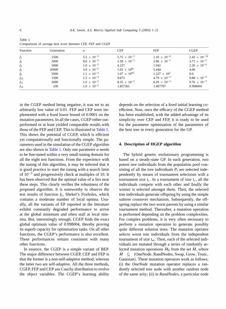
Table 1Comparisons of average best score between CEP, FEP and CGEP
Function Generation α CEP FEP CGEP
f1 1500 5.5× 10⁻³ 5.75 × 10⁻² 1.10 × 10⁻⁴ 2.43 × 10⁻¹⁶
f2 2000 8.0× 10⁻⁵ 2.58 × 10⁻³ 2.06 × 10⁻¹ 3.72 × 10⁻⁵
f3 5000 1.0× 10⁻² 4.227 1.042 2.20× 10⁻⁶
f5 20000 3.0× 10⁻⁵ 1.03 × 1001 5.444 4.00f9 5000 1.1× 10⁻³ 1.07 × 1002 1.227× 10² 0.0f10 1500 1.5× 10⁻³ 9.675 4.79× 10⁻³ 9.88 × 10⁻⁴
f11 2000 1.0× 10⁻² 8.35 × 10⁻¹ 6.29 × 10⁻² 9.76 × 10⁻³
f14 100 1.0× 10⁻² 1.857361 1.407797 0.998004
in the CGEP method being negative, it was set to anarbitrarily low value of 0.01. FEP and CEP were im-plemented with a fixed lower bound of 0.0001 on themutation parameters. In all the cases, CGEP either out-performed or at least yielded comparable results withthose of the FEP and CEP. This is illustrated inTable 1.This shows the potential of CGEP, which is efficientyet computationally and functionally simple. The pa-rameters used in the simulation of the CGEP algorithmare also shown inTable 1. Only one parameterα needsto be fine-tuned within a very small tuning domain forall the eight test functions. From the experience withthe tuning of this algorithm, it may be inferred that itis good practice to start the tuning with a search limitof 10−5 and progressively check at multiples of 10. Ithas been observed that the optimal value ofα lies nearthese steps. This clearly verifies the robustness of theproposed algorithm. It is noteworthy to observe thetest results of functionf5, Shekel’s Foxholes, whichcontains a moderate number of local optima. Usu-ally, all the variants of EP reported in the literatureexhibit constantly degraded performance to arriveat the global minimum and often stall at local min-ima. But, interestingly enough, CGEP finds the exactglobal optimum value of 0.998004, thereby provingits superb capacity for optimisation tasks. On all otherfunctions, the CGEP’s performance is also excellent.These performances remain consistent with manyother functions.
In essence, the CGEP is a simple variant of BEP.The major difference between CGEP, CEP and FEP isthat the former is a non-self-adaptive method, whereasthe latter two are self-adaptive. All the three methods,CGEP, FEP and CEP use Cauchy distribution to evolvethe object variables. The CGEP’s learning ability
depends on the selection of a fixed initial learning co-efficient. Now, once the efficacy of the CGEP methodhas been established, with the added advantage of itssimplicity over CEP and FEP, it is ready to be usedfor the parameter optimisation of the parameters ofthe best tree in every generation for the GP.
4. Description of HGEP algorithm
The hybrid genetic evolutionary programming isbased on a steady-state GP. In each generation, twopotent tree individuals from the population pool con-sisting of all the tree individualsPt are selected inde-pendently by means of tournament selections with atournament sizetc. In a tournament of sizetc, all theindividuals compete with each other and finally thewinner is selected amongst them. Then, the selectedtree individuals generate offspring by using the simplesubtree crossover mechanism. Subsequently, the off-spring replace the two worst parents by using a similartournament method. Thereafter, a mutation operationis performed depending on the problem complexities.For complex problems, it is very often necessary toperform a mutation operation to generate possiblyquite different solution trees. The mutation operatorselects worst tree individuals from the independenttournament of sizetm. Then, each of the selected indi-viduals are mutated through a series of randomly se-lected mutation operationsM0 from the setM, whereM ⊆ {OneNode,RandNodes,Swap,Grow,Trunc,Gaussian}. These mutation operators work as follows:(i) the OneNode mutation operator replaces a ran-domly selected tree node with another random nodeof the same arity; (ii) inRandNodes, a particular node
A.K. Swain, A.S. Morris / Applied Soft Computing 3 (2003) 1–21 7
in a tree is replaced by a random node of the samearity with a very low probability; (iii) theSwap mu-tation operator swaps the arguments of a randomlyselected node of arity more than one; (iv) then, theGrow operator selects a terminal node randomly, andreplaces that with a randomly generated subtree ofpre-specified size; (v) theTrunc mutation operatorrandomly selects a function node and replaces thecomplete subtree starting at that node with a terminalnode; (vi) then, theGaussian operator acts on a ran-domly selected numerical terminal node, and perturbsthat with a Gaussian variate of mean zero and stan-dard deviation 0.1. The number of mutation operatorsare selected as per a Poisson variate. To gain a betterunderstanding of the action of these mutation opera-tors, let the Poisson variate be 3. Now, three mutationoperators will be selected randomly with replacementfrom the mutation setM. Suppose, the randomly se-lected three mutation operators areOneNode, GrowandGaussian. Then, the action of all the three muta-tion operators on a pre-selected tree individualpm
t toprocreate an offspring om
t can be given as follows:
omt = Gaussian(Grow(OneNode(pm
t ))),
where the superscript ‘m’ indicates that it is a mutationrelated operation. Here, the offspring directly replacesits parent.
Now, the best individualpbt in the population pool
Pt is selected. Then, CGEP works on a single indi-vidual p1 = {p1j|j ∈ (1, . . . , n0)}, which is formedwith the numerical nodes (constant terminal nodes) ofpb
t . Thus, the sizen0 of this individual is not a con-stant, but depends on the number of numerical nodes inthe best tree individualpb
t . Subsequently,λ offspringare generated fromp1 by perturbing its object vari-ables by a Cauchy variate of mode zero and median(α/n0)
√f(p1). Then, a stochastic tournament selec-
tion with ‘c’ number of competitors is used to decidethe individual to be used to construct the new and morepotent individual treepn
t with the same structure asthat ofpb
t . Finally,pnt replaces the worst tree individ-
ual in the entire population pool of tree individualsPt.Then, the new pool of tree individuals after crossover,mutation and CGEP optimisation is ready for the nextgeneration. The complete pseudo-code of the HGEPalgorithm is shown inTable 2.
5. Hybrid genetic evolutionary programmingfor symbolic regression
5.1. Test problems
After the development of the HGEP algorithm, itsperformance on standard problems must be testedbefore it can be applied to any complex non-linearsystem. For the verification of the potential of HGEP,two test problems of symbolic regression have beenchosen. The first test problem is a single input regres-sion problem, whereas the second one is a two-inputregression problem. The second problem was selectedto study the effects of multiple inputs on the perfor-mance of different GP-based algorithm. Both thesetest problems are described below.
5.1.1. Test problem 1: one-input symbolic regressionGiven a finite input–output dataset from the equa-
tion, y = 2.719x2 + 3.14161x, the goal is to find theunderlying model from the dataset.
5.1.2. Test problem 2: two-input symbolic regressionGiven a finite input–output dataset from the equa-
tion, z = x2 + y2, the goal is to find the underlyingmodel from the dataset.
5.2. Experimental set-up
5.2.1. Test problem 1: one-input symbolic regressionFor this problem, 20 input–output data points in
the range between−1 and 1 were selected randomly.Generation of random tree structures and subsequentmanipulation of these trees was performed usingsteady-state GP and HGEP method. Initial trees weregenerated using a grow method. The function andterminal sets were:F = {+,−,×, /} and T ={x,U(−1,1)}, whereU(−1,1) is a random numberbetween−1 and 1. The parameters used for the GPpart of the HGEP for this problem are shown inTable 3and the parameters for the CGEP to optimizethe ephemeral constants are shown inTable 4. CGEPused a stochastic (1+ 10) selection method.
5.2.2. Test problem 2: two-input symbolic regressionSimilar to the single-input regression problem, a
steady-state GP and HGEP were used. The initial

8 A.K. Swain, A.S. Morris / Applied Soft Computing 3 (2003) 1–21
Table 2Pseudo-code of hybrid genetic evolutionary programming (HGEP) algorithm
Given:GP parameters:A function setF and a terminal setT , probability of crossover, probability of mutation for all node mutation, probability of
terminal node selection, Poisson mean, tournament size for parent selection for crossover (tc) and mutation (tm), treeinitialisation method (grow, full or ramped-half-and-half), tree population sizeµt, number of fitness cases, maximum treedepth after crossover/mutation, maximum size of a mutant subtree
EP parameters:Learning coefficientα, EP population sizeµ, number of iterations, number of offspringλ, number of competitionc
Step 1.Initialisation:Initialise a population poolPt for the GP, consisting of tree individualsfor i := 1 to µt do
pt[i]:= randomly generate tree individuals;a
wherept[i] represents theith individual tree;
Step 2.Evaluation:Evaluate the individualsfor i := 1 to µt do
Evaluate (pt[i]); //assign a fitness value to each tree individual
Step 3.Recombination (subtree crossover):(i) Select two parents for crossover
Select randomly a group oftc individuals comp[i] ∀i ∈ {1, . . . , tc} from the population poolPt
for i := 1 to tc doir = an integer random number∈ U(0, µt);
comp[i] = pt[ir];pc1t = comp[1];for i := 1 to tc do
if (f(pc1t ) < f(comp[i]))pc1t = comp[i];Similarly, select the second parent for crossoverpc2t ;
(ii) Select crossover sitescn1 = randomly select a node onpc1tcn2 = randomly select a node onpc2t
(iii) Exchange subtrees with root nodescn1 andcn2 betweenpc1t andpc2t to generate two offspringoc1t and oc2t(iv) Replacement of two tree individuals fromPt with offspring oc1t and oc2t
Select the worst individual to be replacedir1 = an integer random number∈ U(0, µt);for i := 1 to tc do
doir2 = an integer random number∈ U(0, µt);
while(ir1 �= ir2);if(f(pt[irl] ) > f(pt[ir2]))ir1 = ir2;pt[ir1] = oc1t ; //replace one individual
Repeat the above process to placeoc2t in the poolPt
Step 4.Mutation:(i) Select parents for mutation operationb
Select randomly a group oftm individuals comp[i] ∀i ∈ {1, tm} from the population poolPt
for i := 1 to tm doir = an integer random number∈ U(0, µt);comp[i] = pt[ir];pm1
t = comp[1];for i := 1 to tm do
if(f(pm1t ) < f(comp[i]))pm1
t = comp[i];Similarly, select the second parent for mutationpm2
t(ii) Calculate the number of mutation operationsγp from a Poisson distribution with a given mean(iii) Generate offspring by mutation

A.K. Swain, A.S. Morris / Applied Soft Computing 3 (2003) 1–21 9
Table 2 (Continued )
while(γp �= 0)Randomly select a mutation operatorM0 from the mutation operator setM|M0 ∈ M ⊆ {OneNode,RandNodes,Swap,Grow,Trunc,Gaussian};
om1t = M0(p
m1t );
γp = γp − 1;Similarly, generate the second offspringom2
t by mutation;(iv) Replacement of offspring
Each offspring replace its parentpm1
t = om1t ;
pm2t = om2
t ;
Step 5.EP calculations:(i) Select the best tree individualpb
t = pt[1];i := 2 to µt do
if(f(pbt ) < f(pt[i]))pb
t = pt[i];(ii) Gather the parameters ofpb
t as a row vector p[1]:{p[1]|p[1][j], ∀j ∈ {1, . . . , no}} with no the number of parameters in the treepbt
(iii) Evaluate (p[1]); //assign a fitness value(iv) Generateλ offspring from p[1] by mutation operation as described belowMutation:Calculate:for j := 1 to no do
s[j] :=√f(pb
t )
no;;
wheres[j] is the scale factor for thejth element, andpbt the fitness of the best tree individualpb
t , which mapspbt → 3
Mutate:for i := 1 to λ do
for j := 1 to no doC=generate a Gaussian random numberC(0,1);p[i+ 1][j] = p[1][j] + Cs[j];
whereC(0,1) represents a standard Cauchy variableEvaluation:Evaluate the offspringfor i := 1 to λ dofor j := 1 to no doEvaluate(p[i][ j]); //assign fitness equal to the fitness with parameters ofpt and the structure ofpb
tSelection:Select one individual from (λ+ 1) individuals by using a stochastic competition comprising of ‘c’ number of participant individuals
for i := 1 to (λ+ 1) dowt[i] := 0.0;for j := 1 to c dot := [(λ+ 1)U(0,1)];
if f(p[i]) ≤ f(p[t])then wt[i] := wt[i] + 1;
where [·] denotes a greatest integer functionfor i := 1 to (λ+ 1) do
for j := 1 to no doSelect the best individual according to its weight wt (i.e. number of wins)
Step 6. If termination condition is not reached return to step 3
a Here, each individual consists of one tree. However, for multiple output systems, parallel trees can be generated analogous to thenumber of object variables per individual in a real coded evolutionary algorithm.
b The number of parents to be mutated can be any number between 0 andµt. However, for this research work, two parents areconsidered to undergo mutation.

10 A.K. Swain, A.S. Morris / Applied Soft Computing 3 (2003) 1–21
Table 3GP parameter values for one-input regression analysis
Parameters Values
Population size 300Probability of leaf selection 0.5Maximum tree depth after crossover 17Probability of mutation 0Number of crossover operations per generation 2Tournament size 4Number of fitness cases 20Initial tree depths 5Crossover probability 1.0Number of generations 200
Table 4CGEP parameter settings for regression analysis
Parameter Value
Population size 1Tournament size 4Learning coefficient (α) 0.0005Number of offspring 5Number of iterations 3
Table 5GP parameter values for two-input regression analysis
Parameter Value
Population size 300Probability of leaf selection 0.5Maximum tree depth after crossover 17Probability of mutation 0Number of crossover operations per generation 2Tournament size 4Number of fitness cases 20Initial tree depths 5Crossover probability 1.0Number of generations 400
Table 6Average best and average mean results of HGEP and GP of one-input regression problem
HGEP GP t-test (GP–HGEP)
Average best Average mean Average best Average mean Average best Average mean
0.984433(0.0474164)
0.822811(0.0345126)
0.868407(0.124908)
0.323265(0.0338958)
3.68467(0.00503883)
31.4079(1.64962E−10)
The bracketed quantities indicate the standard deviation for HGEP and GP, and fort-test, these indicate significance values.
training set of 20 independent data points was se-lected randomly within the open interval (−1, 1). Theparameters used for the GP part of the HGEP areillustrated inTable 5. However, the parameters usedfor the EP part of HGEP are kept the same as forsingle-input regression, as shown inTable 4.
The fitness of an individual tree has been calculatedas the sum-square error of all the fitness cases used tobuild the model. The overall fitness can be expressedas follows:
Fitnor = 1
1 + Fitind
where Fitnor is the normalised overall fitness and in-dividual tree fitness
Fitind =m∑i=1
e2i
with m being the number of fitness cases.
6. Results
6.1. Test problem 1: one-input symbolic regression
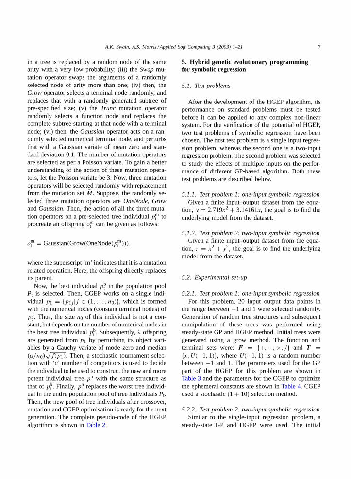
All the results of HGEP have been compared witha simple GP method. The average best and averagemean results of 10 independent runs of HGEP and GPare shown inTable 6. The correspondingt-test resultsare also included inTable 6. The t-test results indi-cate the statistical significance of the results obtainedfrom the GP and HGEP methods in 10 different trials.When thet-values are negative it suggests that the firstof the two methods under test is better than the sec-ond one. The convergence characteristics of the aver-age best and average mean results of both HGEP andGP are shown inFig. 1. It is clear fromFig. 1 that
A.K. Swain, A.S. Morris / Applied Soft Computing 3 (2003) 1–21 11
Fig. 1. Average best and mean characteristics of HGEP and GP methods for one input symbolic regression problem.
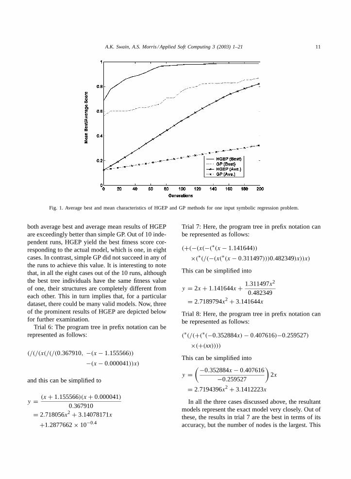
both average best and average mean results of HGEPare exceedingly better than simple GP. Out of 10 inde-pendent runs, HGEP yield the best fitness score cor-responding to the actual model, which is one, in eightcases. In contrast, simple GP did not succeed in any ofthe runs to achieve this value. It is interesting to notethat, in all the eight cases out of the 10 runs, althoughthe best tree individuals have the same fitness valueof one, their structures are completely different fromeach other. This in turn implies that, for a particulardataset, there could be many valid models. Now, threeof the prominent results of HGEP are depicted belowfor further examination.
Trial 6: The program tree in prefix notation can berepresented as follows:
(/(/(x(/(/(0.367910, −(x− 1.155566))
−(x− 0.000041))x)
and this can be simplified to
y = (x+ 1.155566)(x+ 0.000041)
0.367910= 2.718056x2 + 3.14078171x
+1.2877662× 10−0.4
Trial 7: Here, the program tree in prefix notation canbe represented as follows:
(+(−(x(−(∗(x− 1.141644))
×(∗(/(−(x(∗(x− 0.311497)))0.482349)x))x)
This can be simplified into
y = 2x+ 1.141644x+ 1.311497x2
0.482349= 2.7189794x2 + 3.141644x
Trial 8: Here, the program tree in prefix notation canbe represented as follows:
(∗(/(+(∗(−0.352884x)− 0.407616)−0.259527)
×(+(xx))))
This can be simplified into
y =(−0.352884x− 0.407616
−0.259527
)2x
= 2.7194396x2 + 3.1412223x
In all the three cases discussed above, the resultantmodels represent the exact model very closely. Out ofthese, the results in trial 7 are the best in terms of itsaccuracy, but the number of nodes is the largest. This
12 A.K. Swain, A.S. Morris / Applied Soft Computing 3 (2003) 1–21
suggests that minimisation of the number of nodes torepresent a problem may not be a good option in thebroader field of tree-based program optimisation.
On the other hand, the best tree in all the 10 in-dependent runs with simple GP was produced in thesixth trial with best fitness value of 0.968983. The cor-responding tree individual has been presented below.
The program tree in prefix notation can be repre-sented as follows:
(+(−(+(xx)∗(−(0.106337x)(+(−0.381775
×(/(x 0.402704))))))(−(/(x 0.472469)0.060648))))
This can be simplified into
y = 2.4832135x2 + 3.0151025x− 0.0200511
Thus, it is clear from these results that HGEP out-performs simple GP on a one-input symbolic regres-sion problem.
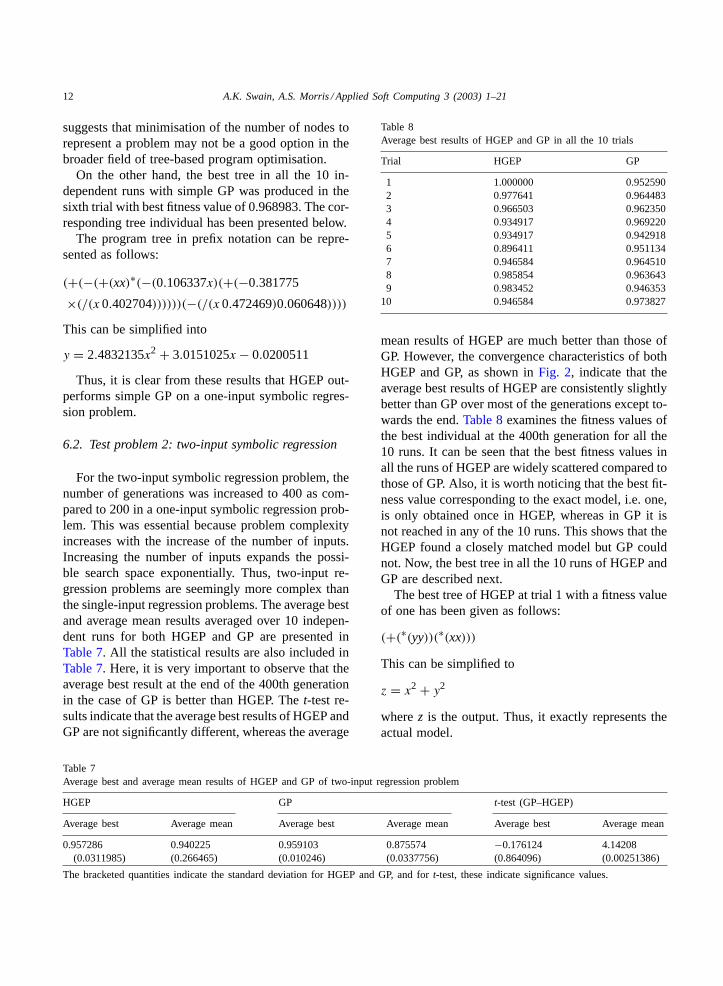
6.2. Test problem 2: two-input symbolic regression
For the two-input symbolic regression problem, thenumber of generations was increased to 400 as com-pared to 200 in a one-input symbolic regression prob-lem. This was essential because problem complexityincreases with the increase of the number of inputs.Increasing the number of inputs expands the possi-ble search space exponentially. Thus, two-input re-gression problems are seemingly more complex thanthe single-input regression problems. The average bestand average mean results averaged over 10 indepen-dent runs for both HGEP and GP are presented inTable 7. All the statistical results are also included inTable 7. Here, it is very important to observe that theaverage best result at the end of the 400th generationin the case of GP is better than HGEP. Thet-test re-sults indicate that the average best results of HGEP andGP are not significantly different, whereas the average
Table 7Average best and average mean results of HGEP and GP of two-input regression problem
HGEP GP t-test (GP–HGEP)
Average best Average mean Average best Average mean Average best Average mean
0.957286(0.0311985)
0.940225(0.266465)
0.959103(0.010246)
0.875574(0.0337756)
−0.176124(0.864096)
4.14208(0.00251386)
The bracketed quantities indicate the standard deviation for HGEP and GP, and fort-test, these indicate significance values.
Table 8Average best results of HGEP and GP in all the 10 trials
Trial HGEP GP
1 1.000000 0.9525902 0.977641 0.9644833 0.966503 0.9623504 0.934917 0.9692205 0.934917 0.9429186 0.896411 0.9511347 0.946584 0.9645108 0.985854 0.9636439 0.983452 0.946353
10 0.946584 0.973827
mean results of HGEP are much better than those ofGP. However, the convergence characteristics of bothHGEP and GP, as shown inFig. 2, indicate that theaverage best results of HGEP are consistently slightlybetter than GP over most of the generations except to-wards the end.Table 8examines the fitness values ofthe best individual at the 400th generation for all the10 runs. It can be seen that the best fitness values inall the runs of HGEP are widely scattered compared tothose of GP. Also, it is worth noticing that the best fit-ness value corresponding to the exact model, i.e. one,is only obtained once in HGEP, whereas in GP it isnot reached in any of the 10 runs. This shows that theHGEP found a closely matched model but GP couldnot. Now, the best tree in all the 10 runs of HGEP andGP are described next.
The best tree of HGEP at trial 1 with a fitness valueof one has been given as follows:
(+(∗(yy))(∗(xx)))
This can be simplified to
z = x2 + y2
wherez is the output. Thus, it exactly represents theactual model.
A.K. Swain, A.S. Morris / Applied Soft Computing 3 (2003) 1–21 13
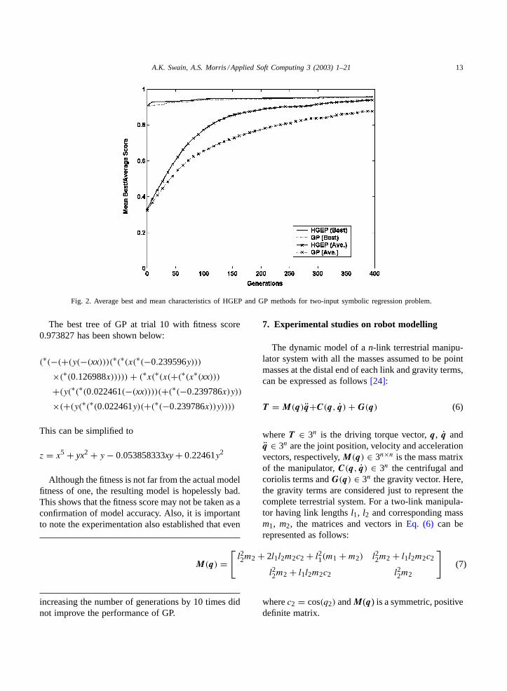
Fig. 2. Average best and mean characteristics of HGEP and GP methods for two-input symbolic regression problem.
The best tree of GP at trial 10 with fitness score0.973827 has been shown below:
(∗(−(+(y(−(xx)))(∗(∗(x(∗(−0.239596y)))
×(∗(0.126988x)))))+ (∗x(∗(x(+(∗(x∗(xx)))
+(y(∗(∗(0.022461(−(xx))))(+(∗(−0.239786x)y))
×(+(y(∗(∗(0.022461y)(+(∗(−0.239786x))y))))
This can be simplified to
z = x5 + yx2 + y − 0.053858333xy + 0.22461y2
Although the fitness is not far from the actual modelfitness of one, the resulting model is hopelessly bad.This shows that the fitness score may not be taken as aconfirmation of model accuracy. Also, it is importantto note the experimentation also established that even
M(q) =[l22m2 + 2l1l2m2c2 + l21(m1 +m2) l22m2 + l1l2m2c2
l22m2 + l1l2m2c2 l22m2
](7)
increasing the number of generations by 10 times didnot improve the performance of GP.
7. Experimental studies on robot modelling
The dynamic model of an-link terrestrial manipu-lator system with all the masses assumed to be pointmasses at the distal end of each link and gravity terms,can be expressed as follows[24]:
T = M(q)q+C(q, q)+ G(q) (6)
whereT ∈ 3n is the driving torque vector,q, q andq ∈ 3n are the joint position, velocity and accelerationvectors, respectively,M(q) ∈ 3n×n is the mass matrixof the manipulator,C(q, q) ∈ 3n the centrifugal andcoriolis terms andG(q) ∈ 3n the gravity vector. Here,the gravity terms are considered just to represent thecomplete terrestrial system. For a two-link manipula-tor having link lengthsl1, l2 and corresponding massm1, m2, the matrices and vectors inEq. (6) can berepresented as follows:
wherec2 = cos(q2) andM(q) is a symmetric, positivedefinite matrix.
14 A.K. Swain, A.S. Morris / Applied Soft Computing 3 (2003) 1–21
C(q, q) =[m2l1l2s2q
22 −m2l1l2s2q1q2
m2l1l2s2q21
](8)
wheres2 = sin(q2).
G(q) =[m2l2gc12 + (m1 +m2)l1gc1
m2l2gc12
](9)
wherec1 = cos(q1) andc12 = cos(q1 + q2).
7.1. Test problems
The following two test problems were used to gen-erate the initial dataset for verifying the potential ofthe proposed HGEP method for extracting the under-lying model.
7.1.1. Test problem 1: single-link robot manipulatorFrom Eq. (6), the equations of motion of a
single-link manipulator can be expressed as follows:
τ1 = l21m1q1 +m1l1gc1 (10)
Now, the joint accelerationq1 can be represented asfollows:
q1 = 1
l21m1(τ1 −m1l1gc1) (11)
Eqs. (10) and (11)involve less complexities comparedto the two-link manipulator described next.
7.1.2. Test problem 2: forward dynamics model oftwo-link robot manipulator
The general form of the equation of motion of amanipulator system is given inEq. (6). For a two-linkmanipulator withEqs. (7)–(9), the forward dynamicsequation can be represented as follows:
q = M−1(q)(T − C(q, q)− G(q)) (12)
This is a highly complex modelling problem due tothe presence of the non-linear coupling between theparameters of the two links of the manipulator.
7.2. Experimental set-up
The experiments on the above two problems wereperformed under quite different conditions. These arediscussed below.
Table 9GP parameter values for single-link manipulator
Parameter Value
Population size 100Probability of leaf selection 0.5Maximum depth after crossover 17Probability of mutation 0Number of crossover operations per generation 2Tournament size 4Number of fitness cases 20Initial tree depths 5Number of generations 300Number of crossover operations per generation 0
7.2.1. Test problem 1: single-link robot manipulatorThe dataset consisting of 20 input–output samples
was generated fromEq. (11)for a random torqueτ1between−5 and 5. Here, a normal grow initialisationmethod was used for generating initial tree individuals.The parameters used for the GP part of the HGEPare illustrated inTable 9. Here, the GP part of theHGEP uses a steady-state GP for extracting the modelfrom the supplied data points. The parameters of theCGEP were kept the same as those inTable 4. Theexperiments were performed on two cases of functionsetsF and terminal setsT . The function and terminalsets are described below.
Case 1. F = {+,−,×, /} and T = {τ1, cos(q1),U(−1,1)}, whereU(−1,1) is a random number be-tween –1 and 1.
Case 2. F = {+,−,×, /, cos} and T = {τ1, q1, U
(−1,1)}.
The parameters of the robotic manipulator system areshown inTable 10.
7.2.2. Test problem 2: forward dynamics model oftwo-link robot manipulator
The model represented inEq. (12) is a highlycomplex and coupled system. The values of joint
Table 10Manipulator parameter setting
Parameter Value
Mass of each links 1 kgAcceleration due to gravity 9.8 m/s2
Lengths of each link 1 m
A.K. Swain, A.S. Morris / Applied Soft Computing 3 (2003) 1–21 15
acceleration associated with any link depend on thetorque, joint velocity, joint angle and masses and linklengths of both the links of the manipulator. Thiscomplicates the selection of the combinations of in-puts to form the initial training dataset. It has alreadybeen shown that the increase in the number of inputsincreases the complexity of the problem and it be-comes hard to get the exact model. Because of this,the number of inputs are relatively high in a two-linkmanipulator problem. In addition, there are equallylarge numbers of possible input patterns that generatedifferent actions of the manipulator. However, for amanipulator system to perform a particular task, afixed pattern of joint and end-effector paths must befollowed. Moreover, a particular task excites onlycertain specific modes of the manipulator. Hence, itis very likely that the dataset used for the modellingtask is biased towards the specific job for which thedata has been collected. This in fact says that it is veryunlikely that a general model for a robotic manipula-tor system can be found. In this work three differentinput–output datasets are generated and tested formodel building.
Case 1 (A single randomly generated sinusoid). Herejoint angles are assumed to follow sinusoidal varia-tions:
qd = qmax(1 − cosωt) (13)
whereqd is the desired joint angle,qmax ∈ U(0,0.2)is the maximum value of the sinusoidal joint variationand ω ∈ U(0,2π) is the angular frequency of thesinusoid. Here,qmax andω were chosen randomly inthe prescribed open interval. A total of 40 data pointshave been generated within a time period of [0,1) foreach of the possible inputs for the model building.
Case 2 (Two randomly generated sinusoids). In thiscase, 20 data points with each selection ofqmax andω were generated. Thus, the entire training datasetgenerated fromEq. (13)total of 40 data points for eachinput. The choice of this number of inputs was madein order to keep the number of fitness cases fixed at avalue of 40 in both the Cases 1 and 2.
Case 3 (Multiple sinusoids). Here, 20 sinusoids ofrandom amplitude and frequency were selected for
Table 11Parameter values for the GP part of the HGEP for two-link ma-nipulator
Parameter Value
Population size 300Probability of leaf selection 0.5Maximum depth after crossover 17Probability of mutation in RandNode 0.05Number of crossover
operations per generation2
Tournament size 4Number of fitness cases 40Initial tree depths (8, 7, 6, 5, 4)Number of generations 16000Number of mutation
operations per generation2
each joint angle variation. The sinusoidal equationused here is given as follows:
qd = 12(q
max)cosωt (14)
UsingEq. (14), 40 data points (torque) were generatedwith qmax varying uniformly and randomly between0 and 3, andω varying between 0 and 2π. Thus, atotal of 800 input–output data points were used to trainthe GP trees. Each tree is allowed to be exposed to aparticular sinusoid for only two generations. Hence,80 generations are required for the GP trees to face allthe data points in the input–output dataset.
In every generation, two individuals were selectedeach for crossover and mutation operation. Theephemeral constants of the best tree in each gen-eration are evolved using CGEP. The function andterminal sets for this problem are:F = {+,−,×, /},T = {τ1, τ2, q1, q2, q1, q2, cos(q1), cos(q2), sin(q1),
sin(q2)}. Then, initial GP trees are generated using aramped half-and-half method. The GP parameters areshown inTable 11. The CGEP parameters are set toexactly the same values as those used in regressionanalysis, and are tabulated inTable 4.
8. Results
It has already been discussed that HGEP outper-forms simple GP on both symbolic regression testproblems. Hence in this section, both HGEP and GPare considered for the one-link manipulator, whereas
16 A.K. Swain, A.S. Morris / Applied Soft Computing 3 (2003) 1–21
Table 12Average best and average mean results of HGEP and GP for one-link robotic manipulator system
Case studies HGEP GP t-test (GP–HGEP)
Average best Average mean Average best Average mean Average best Average mean
Case 1 0.923908(0.240179)
0.782405(0.234272)
0.639269(0.297452)
0.073540(0.036198)
2.01015(0.0753096)
9.24509(6.85E−06)
Case 2 0.470207(0.335021)
0.344297(0.318587)
0.207283(0.275412)
0.036934(0.016351)
1.98864(0.0779675)
3.1308(0.0120616).
The bracketed quantities indicate the standard deviation for HGEP and GP, and fort-test, these indicate significance values. Case 1 is withpre-processed inputs and Case 2 is without any pre-processed inputs.
only HGEP has been used to extract the model forthe complex two-link manipulator system. For all thetests, the best result of the 10 independent runs ofHGEP and GP has been chosen as the final model ofthe system.
8.1. Test problem 1: single-link robot manipulator
Case 1 considers pre-processed inputs, i.e. the inputjoint angle is pre-processed through a cosine functionbefore being fed to the individual trees. In the contextof neural networks, Lewis et al.[25,26] showed thatinputs pre-processed with system knowledge impartless training burden on the network, and thus resultin better overall performance. Whereas, in Case 2, the
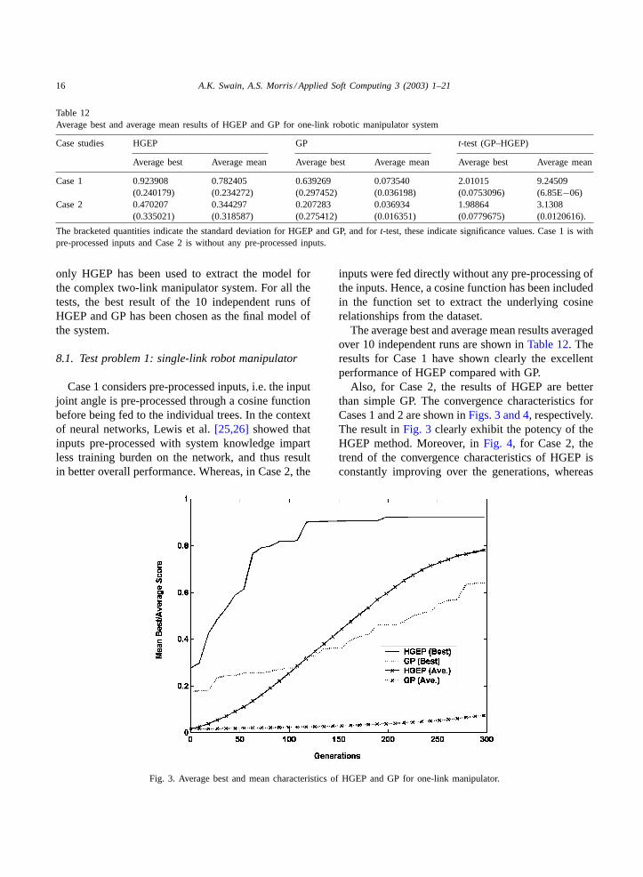
Fig. 3. Average best and mean characteristics of HGEP and GP for one-link manipulator.
inputs were fed directly without any pre-processing ofthe inputs. Hence, a cosine function has been includedin the function set to extract the underlying cosinerelationships from the dataset.
The average best and average mean results averagedover 10 independent runs are shown inTable 12. Theresults for Case 1 have shown clearly the excellentperformance of HGEP compared with GP.
Also, for Case 2, the results of HGEP are betterthan simple GP. The convergence characteristics forCases 1 and 2 are shown inFigs. 3 and 4, respectively.The result inFig. 3 clearly exhibit the potency of theHGEP method. Moreover, inFig. 4, for Case 2, thetrend of the convergence characteristics of HGEP isconstantly improving over the generations, whereas
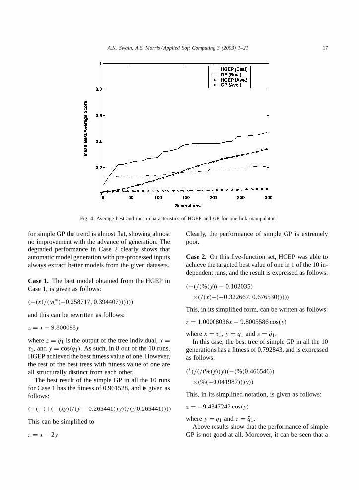
A.K. Swain, A.S. Morris / Applied Soft Computing 3 (2003) 1–21 17
Fig. 4. Average best and mean characteristics of HGEP and GP for one-link manipulator.
for simple GP the trend is almost flat, showing almostno improvement with the advance of generation. Thedegraded performance in Case 2 clearly shows thatautomatic model generation with pre-processed inputsalways extract better models from the given datasets.
Case 1. The best model obtained from the HGEP inCase 1, is given as follows:
(+(x(/(y(∗(−0.258717,0.394407))))))
and this can be rewritten as follows:
z = x− 9.800098y
wherez = q1 is the output of the tree individual,x =τ1, andy = cos(q1). As such, in 8 out of the 10 runs,HGEP achieved the best fitness value of one. However,the rest of the best trees with fitness value of one areall structurally distinct from each other.
The best result of the simple GP in all the 10 runsfor Case 1 has the fitness of 0.961528, and is given asfollows:
(+(−(+(−(xy)(/(y − 0.265441))y)(/(y 0.265441))))
This can be simplified to
z = x− 2y
Clearly, the performance of simple GP is extremelypoor.
Case 2. On this five-function set, HGEP was able toachieve the targeted best value of one in 1 of the 10 in-dependent runs, and the result is expressed as follows:
(−(/(%(y))− 0.102035)
×(/(x(−(−0.322667,0.676530)))))
This, in its simplified form, can be written as follows:
z = 1.00008036x− 9.8005586 cos(y)
wherex = τ1, y = q1 andz = q1.In this case, the best tree of simple GP in all the 10
generations has a fitness of 0.792843, and is expressedas follows:
(∗(/(/(%(y))y)(−(%(0.466546))
×(%(−0.041987)))y))
This, in its simplified notation, is given as follows:
z = −9.4347242 cos(y)
wherey = q1 andz = q1.Above results show that the performance of simple
GP is not good at all. Moreover, it can be seen that a

18 A.K. Swain, A.S. Morris / Applied Soft Computing 3 (2003) 1–21
higher value of fitness close to one may not necessarilygenerate a good model. At least until now, it is clearthat a fitness value of one generates a quite accuratemodel.
8.2. Test problem 2: forward dynamics model oftwo-link robot manipulator
Here, for all the model description, the termsx, y,a, b, c, d, e, f, g andh denoteτ1, τ2, q1, q2, q1, q2,cos(q1), cos(q2), sin(q1) and sin(q2), respectively.
Case 1. The evolved tree forq1 is expressed as fol-lows:
(A+ B + CD)E
where
A= g
f 13;
B= 0.504441
(a4
e4f 11+ ea
0.498535(ga − e)
);
C= f + C′ + C′′
with
C′ = a
f 8+ 0.773701
(g
f 5− ef 4
a
);
C′′ = a
f 6
{f − 3.893349
(a2 − e
a
)}− ef 9
a
D = e+ b; E =(g
f 14− ef13
g
)
The second outputq2 in its simplified form, can beexpressed asq2 = 0.102055e+ 0.0346979.
Case 2. The evolved tree forq1, in its simplified form,can be expressed as follows:
q1 = g− 5.121055af
−{(d − 0.039398+ d + xb
A
)+ B
}C +D
where
A = g(e− 0.289854)
xb+ xb
c − 0.091650A′ + A′′
with
A′ =(a
c+ xb
e− 0.289854
)g;
A′′ = c + d(a+ b− e− 2f + 2g− 6.388320);B = (2a− f)
{f +
(g
b+ c + 0.45697
)
×(
bg
eb+ bc + 2b+ c + 0.045697
)};
C = c
c + g+ f + 2ceg − 1.026757;
D = 2g− f − 0.328311b
f − bg+ d − c(d + g)
×(2g− f − 0.212758)+ d
+ xbe2(b+ c − 0.141237)
(b+ c + xb − 141237)g+D′
with
D′ = e(b+ c − 0.141237)(c − 0.045493)
The second outputq2, in its simplified form, can beexpressed as follows:
q2 = ad + 2h+ 2a2d + (a+ 0.3599003c
−0.6119268)
(ad
c
)+ ac3d + 2adh
−1.153011ad + 0.12511
Case 3. The evolved tree in this case is very large,and in readable form it can be represented as follows:
q1 = (A− BC)D
(E + F)G
whereA, B, C, D, E, F andG are functions of manip-ulator parameters and are expressed as
A= eb + d
x− (b/(ef − y));
B= 0.4915a
(g− b+ h
b
)(f − b);
C= d + y − 0.406856
0.406856;
D= −by(x+ 2.19286)
(b/y)+ x− y;
E=(
−1.40468+ d + by
0.308786
)e
b; F = by
cef;
G= d + y − 0.406856
0.406856
A.K. Swain, A.S. Morris / Applied Soft Computing 3 (2003) 1–21 19
For this case, the average score is 0.802978 and thebest score is 0.999921. Similar results were noted forq2.
All the experiments on the two-link manipulatorwere performed with pre-processed inputs. In Case 1,the evolved model is much simpler in structure com-pared to other two cases. This is mostly because of theuse of the data points from a single sinusoid. More-over, in all the cases, the results do not provide theactual model from which the dataset was generated,although the fitness scores are relatively high. Thissuggests that the resultant structure in these cases isbiased by some dominant modes of the training data,and thus drags the system to that particular mode. Itthus appears that the HGEP-based modelling schemeprovides a local model rather than a global one. Thisprovision of more clarity to the underlying situation isone of the most important features of GP. In contrastto neural networks, the clear transparent structure ofGP is able to provide such typical model characteris-tics very efficiently. This unique power of GP-basedtechniques can be utilised as a framework for globaldata-based modelling. However, in the present context,the results above clearly demonstrate that the HGEPmethod is not able to find the exact model of a two-linkmanipulator system. Thus, it is expected that it willalso not work for more complex multi-arm manipula-tor systems.
9. Discussion
The results presented inSection 6can imply that itis necessary for an accurate and precise model gen-erated automatically from a given dataset to have afitness score that is the same as the original systemor the actual model, but it is not a sufficient condi-tion to obtain an exact or a very close approximationof the exact model. This can, otherwise, be stated asthat a given model derived from a desired dataset hav-ing fitness same as the actual model may not alwaysreplicate the actual system.
Thus, an inappropriately generated input–outputdataset used for model generation may yield a localmodel whose fitness is the same as that of the actualmodel. A local model provides a biased model ofthe system as in the case of a two-link manipulator,
where in Case 1 (Section 6), the model promptlyachieves the desired highest level of fitness value.In spite of the high value of the fitness, the modelis far from the correct one. This clarity of local andglobal (actual) model always remains hidden in allnon-transparent modelling methods like neural net-works. Thus, GP-based methods in general provide abetter picture of the system and help in understandingthe internal dynamics of the system.
Moreover, during the process of simulation of theautomatic generation of the dynamic models, the fol-lowing important points have been experienced.
• During the learning process, the HGEP methoddid not include all the designated inputs from theterminal set into the model. Thus, the resultantmodel becomes biased toward some particular lo-cal structure of the system. It is quite obvious thatthe input–output data collected for training alwayspertains to some particular task. Hence, the modelfrom this dataset will always be biased towardsthat task. Thus, in particular, it is quite difficult toobtain a global system model.
• Global models are likely to be obtained from acompletely randomly generated input and outputset. However, a completely randomly generateddataset with many input and output variables in-creases the feasible search space enormously. Thus,it is almost impossible to obtain any useful modelfrom a completely random input–output datasetwith many inputs. Due to this reason, for a sim-ple system like a single-link manipulator wherethe number of inputs are very few, the completelyrandom input–output dataset produced the exactmodel. Whereas, when a two-link manipulatorsystem with many input variables was tested withcomplete random input–output datasets, the fitnessscore never exceeded 0.1 with finite populationsize and learning time. This prohibits any possi-bility of obtaining good models for a system withmany inputs from randomly generated input–outputdatasets within a limited time with finite populationsize. Due to this reason, natural sinusoidal type ofinput variations were chosen to train the HGEP inorder to obtain the mathematical model.
• It has been shown that the HGEP method used fordata-based intelligent modelling is not capable of re-producing the actual model for even a two-link, rigid
20 A.K. Swain, A.S. Morris / Applied Soft Computing 3 (2003) 1–21
manipulator system. However, it provides greaterinsight into the internal structure of the problem,compared to other data-based modelling methods,thereby leading to a new dimension in the anal-ysis of intelligent data-based modelling methods.Hence, conventional mathematical models[24–26],although requiring high mathematical skills, are theonly way to represent complex robotic manipulatorsystems. Thus, it is suggested from the results de-scribed in this paper that conventional mathematicalmodelling methods are the only choice at present forthe simulation and control operations of complex,non-linear manipulator systems until the develop-ment of a highly efficient intelligent data-based al-gorithm as an automatic model generator.
10. Conclusions
This paper has described a hybrid GP and EP(HGEP) method for modelling the task. GP has beenused to find an optimal model structure and EPevolves the ephemeral constants contained within aparticular GP model structure to make the underly-ing GP model structure more robust. To speed upthe overall process of the model evolution, suitablemodifications to the basic EP technique have beenperformed that use Cauchy distribution instead of theusual normal distribution of BEP. Thus, this yield avery fast EP method, named here as Cauchy-guidedEP method. In order to reduce the computational bur-den, only one tree individual per generation has beenchosen to better exploit its underlying structure. Dueto the use of a single tree, the CGEP method dealswith only one row vector of numerical parameters ofthe selected tree. Hence, a (1+λ) stochastic selectionstrategy has been used for updating the numericalparameters of the selected tree individual.
For complex problems, both crossover and muta-tion operators were used to exploit the program searchspace. The mutation operation used here consists of aseries of mutation operators forming a mutation set. APoisson variate has been used to select the number ofmutation operators to be used for the overall mutationof the selected tree individual. Then, the best model ofeach generation is picked up, and its ephemeral con-stants are optimised for best performance. Then, theworst tree in that generation is replaced by the CGEP
optimised tree. Thus, in each generation, the best treeof GP coexists with its subsequent optimised suppos-edly more fit tree.
It has been shown experimentally that, for complexproblems, it is always necessary to incorporate systemknowledge into the input–output dataset. For a robotmanipulator system, pre-processing of the input databy means of the cosine and sine functions greatly im-proves the overall performance. Hence, it is suggestedhere that system knowledge should always be incorpo-rated into the input–output dataset to reduce the pres-sure on the optimisation method, thereby helping theunderlying method to yield better results.
It has also been emphasised that, for a proper model,it is necessary for the fitness of the evolved model tobe same as the fitness of the actual model, but this isnot a sufficient condition to produce an exact systemmodel.
More importantly, it has been shown, whilst thatthe HGEP method performed better than the conven-tional tree-coded GP method on many simple modelgeneration tasks including a model for single-linkmanipulator system, it could not generate the exactforward dynamics model for a two-link manipulatorsystem.
References
[1] A. Eskandarian, N.E. Bedewi, B.M. Kramer, A.J. Barbera,Dynamic modelling of robotic manipulators using artificialneural network, J. Robotic Syst. 11 (1) (1994) 41–56.
[2] K. Hunt, G. Irwin, K. Warwick, Neural Network Engineeringin Dynamic Control Systems, Spinger-Verlag, London, 1995.
[3] O. Omidvar, D.L. Elliott, Neural Systems for Control,Academic Press, New York, 1997.
[4] D. Psaltis, A. Sideris, A.A. Yamamura, A multilayered neuralnetwork controller, IEEE Control Systems Magazine, April1988, pp. 17–21.
[5] P. Marenbach, K.D. Bettenhausen, S. Freyer, U. Nieken,H. Rettenmaier, Data driven structured modelling of abiotechnological fed-batch fermentation by means of geneticprogramming, in: Proceedings of the Institution of MechanicalEngineers, J. Syst. Control Eng. (1997).
[6] P. Marenbach, M. Brown, Evolutionary versus inductiveconstruction of neuro-fuzzy systems for bioprocessmodelling, in: A.M.S. Zalzala (Ed.), Proceedings of theSecond International Conference on Genetic Algorithmsin Engineering Systems: Innovations and ApplicationsGALESIA, University of Strathclyde, Glasgow, UK, 1997,pp. 320–325.
A.K. Swain, A.S. Morris / Applied Soft Computing 3 (2003) 1–21 21
[7] H. Hiden, M. Willis, B. McKay, G. Montague, Non-linearand direction dependent dynamic modelling using geneticprogramming, in: J.R. Koza, K. Deb, M. Dorigo, D.B.Fogel, M. Garzon, H. Iba, R.L. Riolo (Eds.), Proceedingsof the Second Annual Conference on Genetic Programming,Stanford University, CA, Morgan Kaufmann, San Francisco,1997, pp. 168–173.
[8] B. McKay, C. Sanderson, M.J. Willis, J. Barford, G. Barton,Evolving a hybrid model of a batch fermentation process,Trans. Inst. Measur. Control (1997).
[9] H. Cao, L. Kang, Z. Michalewicz, Y. Chen, A two-levelevolutionary algorithm for modelling system of ordinarydifferential equations, in: Proceedings of the Third AnnualConference on Genetic Programming, 1998, pp. 17–22.
[10] L.M. Howard, J. D’Angelo, The GA-P: a genetic algorithmand genetic programming hybrid, IEEE Expert, June 1995,pp. 11–15.
[11] O. Castillo, P. Melin, A new-fuzzy–fractal–genetic method forautomated mathematical modelling and simulation of roboticdynamic systems, Proc. IEEE Fuzzy Syst. (1998) 1182–1187.
[12] H. Cao, L. Kang, Y. Chen, Evolutionary modelling of ordinarydifferential equations for dynamic systems, in: Proceedingsof the Genetic and Evolutionary Computation Conference(GECCO-99), 1999, pp. 959–965.
[13] D.E. Goldberg, Genetic Algorithms in Search, Optimisationand Machine Learning, Addison-Wesley, Reading, 1998.
[14] H.P. Schwefel, Numerical Optimisation of ComputingModels, Wiley, Chichester, UK, 1981.
[15] D.B. Fogel, Evolutionary Computation: Towards a NewPhilosophy of Machine Intelligence, IEEE Press, 1995.
[16] L.J. Fogel, A.J. Owens, M.J. Walsh, Artificial IntelligenceThrough Simulated Evolution, Wiley, New York, 1966.
[17] X. Yao, Y. Liu, G. Lin, Evolutionary programming madefaster, IEEE Trans. Evol. Comput. 3 (2) (1999) 82–102.
[18] A.K. Swain, A.S. Morris, Performance Improvement ofSelf-Adaptive Evolutionary Methods with a Dynamic LowerBound, Int. J. Inform. Process. Lett. (2001).
[19] T. Bäck, Evolutionary Algorithms in Theory and Practice,Oxford University Press, New York, 1996.
[20] J.R. Koza, Genetic Programming: On the Programming ofComputers by Natural Selection, MIT Press, Cambridge, MA,1992.
[21] W. Banzaf, P. Nordin, R.E. Keller, F.D. Francone, GeneticProgramming: An Introduction. Morgan Kaufmann, NewYork, USA, 1998.
[22] A.K. Swain, A.M.S. Zalzala, An overview of geneticprogramming: current trends and applications, Research reportno. 147, University of Sheffield, UK.
[23] N.L. Johnson, S. Kotz, N. Balakrishnan, ContinuousUnivariate Distributions, vol. 1, Wiley, New York, USA, 1994.
[24] J.J. Craig, Introduction to Robotics: Mechanics and Control,Addison-Wesley, Reading, 1989.
[25] F.L. Lewis, K. Liu, A. Yesildirek, Neural net robot controllerwith guaranteed tracking performance, IEEE Trans. NeuralNetworks 6 (3) (1995) 703–715.
[26] F.L. Lewis, S. Jagannathan, A. Yesildirek, Neural NetworkControl of Robot Manipulators and Nonlinear Systems. Taylor& Francis, London, 1999.
Anjan Kumar Swain, received his bachelors of science degreein electrical engineering in 1988, masters of science in engineer-ing in 1991 from Regional Engineering College, Rourkela, India,and PhD degree from the University of Sheffield, UK in 2001. Heworked with Electrical Engineering Department of Regional Engi-neering College Rourkela, India, from 1988 to 1989 and 1991 to1992. Subsequently, he worked with Ramco Electronics Division,Madras, India from 1992 to 1993 as a real-time process controlsoftware engineer. After that he joined as a lecturer in the Elec-trical Engineering Department of Indira Gandhi Institute of Tech-nology, Orissa, India. He has over 50 publications in journals andconferences. He is the recipient of the national best young teacheraward for the year 1996 in India. His current research interestsinclude evolutionary computing methods, evolving networks, dy-namics and control of multi-arm robotic manipulator systems. Heserves as a reviewer of journals and conferences including IEEETransactions on System, Man and Cybernetics.
Alan S. Morris was educated in UK and graduated with a BEngdegree in electrical and electronic engineering from Sheffield Uni-versity in 1969. After 5 years of employment with British Steelas a research and development engineer in control system appli-cations, he returned to Sheffield University to carry out researchin electric arc furnace control, for which he was awarded the de-gree of PhD in 1978. Since that time, he has been employed as alecturer, and more recently senior lecturer, at Sheffield, where henow holds the position of Director of Undergraduate Studies. Hismain research interests lie in robotics, and he is now the author ofover 100 refereed research papers. Professionally, he is a Fellowof the Institute of Measurement and Control and a Member of theInstitution of Electrical Engineers, and participates as a memberof technical panels and organiser of conferences.