Embed Size (px)
Citation preview
Sensors 2008, 8, 7753-7782; DOI: 10.3390/s8127753
sensors ISSN 1424-8220
www.mdpi.com/journal/sensors
Article
An Energy-Efficient Secure Routing and Key Management Scheme for Mobile Sinks in Wireless Sensor Networks Using Deployment Knowledge
Le Xuan Hung 1,*, Ngo Trong Canh 1, Sungyoung Lee 1,*, Young-Koo Lee 1 and Heejo Lee 2
1 Dept. of Computer Engineering, Kyung Hee University, Seocheon, Giheung, Yongin, Gyeonggi,
Korea; E-Mails: [email protected]; [email protected] 2 Dept. of Computer Science and Engineering, Korea University, Anam-dong, Seongbuk-gu, Seoul
136-713, Korea; E-Mail: [email protected]
* Author to whom correspondence should be addressed; E-Mails: [email protected];
[email protected]; Tel.: +82-31-201-2514; Fax: +82-31-202-2520
Received: 7 October 2008; in revised form: 10 November 2008 / Accepted: 3 December 2008 /
Published: 3 December 2008
Abstract: For many sensor network applications such as military or homeland security, it
is essential for users (sinks) to access the sensor network while they are moving. Sink
mobility brings new challenges to secure routing in large-scale sensor networks. Previous
studies on sink mobility have mainly focused on efficiency and effectiveness of data
dissemination without security consideration. Also, studies and experiences have shown
that considering security during design time is the best way to provide security for sensor
network routing. This paper presents an energy-efficient secure routing and key
management for mobile sinks in sensor networks, called SCODEplus. It is a significant
extension of our previous study in five aspects: (1) Key management scheme and routing
protocol are considered during design time to increase security and efficiency; (2) The
network topology is organized in a hexagonal plane which supports more efficiency than
previous square-grid topology; (3) The key management scheme can eliminate the impacts
of node compromise attacks on links between non-compromised nodes; (4) Sensor node
deployment is based on Gaussian distribution which is more realistic than uniform
distribution; (5) No GPS or like is required to provide sensor node location information.
Our security analysis demonstrates that the proposed scheme can defend against common
attacks in sensor networks including node compromise attacks, replay attacks, selective
forwarding attacks, sinkhole and wormhole, Sybil attacks, HELLO flood attacks. Both
OPEN ACCESS
Sensors 2008, 8
7754
mathematical and simulation-based performance evaluation show that the SCODEplus
significantly reduces the communication overhead, energy consumption, packet delivery
latency while it always delivers more than 97 percent of packets successfully.
Keywords: Secure routing, key management, sensor networks, sink mobility, deployment
knowledge
1. Introduction
Wireless Sensor Networks (WSNs) comprises of a large number of sensor nodes that are densely
deployed either inside the phenomenon or very close to it. In sensor networks, a source is defined as a
sensor node that detects a stimulus, which is a target or an event of interest, and generates data to
report the stimulus. A sink is defined as a user collecting these data reports from the sensor network.
In many sensor network applications such as military, homeland security or environmental
surveillance, it is necessary for users (sinks) to access sensor networks while they are moving. For
example, in a battle- field a soldier with a PDA in hand might continuously collect an enemy tank’s
movement information while he is moving.
Sink mobility brings new challenges to secure routing in large-scale sensor networks. To maintain a
dissemination rout, a mobile sink has to constantly propagate its current location information to all
sensor nodes. That introduces significantly communication overhead. Furthermore, intermediate nodes
on the new rout have to discover their neighbors and exchange secret information to establish a secure
communication. That also introduces more computation and communication overhead.
A number of routing protocols have been proposed for WSNs such as LEACH [1], SecRout [2],
SEEM [3], SeRINS [4], TTSR [23]. However, these works do not take into account of sink mobility
and their routing paths remains static. So they are not suitable to work in such mobile sink
circumstances. Several studies have considered the scalability and efficiency of data dissemination
from multiple sources to mobile sinks such as TTDD [17], Directed Diffusion (DD) [18], SAFE [5],
SEAD [6], Declarative routing protocol [7], and GRAB [8]. However, the authors mainly focused on
energy efficiency. These approaches are very vulnerable from many attacks in sensor network routing
such as spoofed, altered, or replayed routing information [9][16], selective forwarding, sinkhole [16],
Sybil [10], wormhole [11], and HELLO flood (unidirectional link) attacks [16]. Also, most of existing
routing protocols consider routing protocols and security schemes (like key management) separately.
As a consequence, it is unsurprising that they are vulnerable to many attacks. It is not trivial to fix the
problem since it is unlikely that a sensor network routing protocol can be made secure by
incorporating security mechanisms after the design has completed. Studies and experiences have
shown that considering security during design time is the best way to provide security and efficiency
for sensor network routing.
In this paper, we propose an energy-efficient secure routing protocol and key management scheme
for mobile sinks in sensor networks, called SCODEplus. This scheme is a significant extension of our
previous work [12][26] in five aspects:
Sensors 2008, 8
7755
(1) Key management scheme and routing protocol are considered during design time to increase
security and efficiency. In our previous study, we focused on the efficiency for the secure
routing protocol with an assumption that the sensor network achieves a key infrastructure from
LEAP+ [14].
(2) The network topology is organized in a hexagonal plane. Compared with our previous square-
grid topology, the hexagonal topology brings more efficiency. It decreases the number of cells,
reduces transmission hops, and increases the number of sleeping nodes to save more energy.
This is because the hexagonal geometry provides the best approximation to circle and covers
the biggest area as compared to the rectangle or triangle. Also, a hexagon has the least
neighboring cells (six) compared with a rectangle (eight) or a triangle (twelve).
(3) The key management scheme can eliminate the impacts of node compromise attacks on links
between non-compromised nodes. Our previous work has a weakness with impacts of nodes
compromise attacks like most existing key management schemes.
(4) Sensor node deployment conforms to Gaussian distribution. In our previous study, we assumed
that all sensor nodes are uniformly distributed. However, this is not realistic and it might raise
unexpected problems when we deploy the protocol in reality.
(5) No GPS (Global Position System) or like is required to provide node’s location information. In
SCODE, we have assumed that sensor nodes need to be aware of their locations. However,
attaching GPS or like increases high cost for sensors, and thus reducing the feasibility of the
deployment. By using deployment knowledge, the proposed scheme can establish a key
infrastructure and end-to-end communication for the sensor network.
The major contributions of this study are then four fold:
(1) We propose a first, novel secure routing protocol and key management scheme supported sink
mobility in WSNs.
(2) Compared with existing approaches, the proposed routing protocol is more energy-efficient,
lower communication overheads, high packet delivery ratio (>97%), and secure against the
common attacks in sensor networks.
(3) Our key management scheme takes advantage of the hexagonal topology and expected location
information not only to reduce the memory cost but also get better resilience against node
compromise attacks. Moreover, the scheme can eliminate the impacts of node compromise
attacks on links between non-compromised nodes.
(4) Intensive theoretical as well as simulation-based analysis and evaluation studies show that the
proposed scheme achieves better security and efficiency than our previous work as well as
other popular approaches like TTDD and DD.
The rest of the paper is organized as follows: Section 2 discusses common attacks in sensor
networks routings. Section 3 contains brief description on the GAF protocol, as it is used as an
underline protocol in our proposal. Section 4 briefly describes our previous study SCODE. Section 5
presents SCODEplus scheme in details including key management scheme and routing protocol. We
analyze security and cost of the scheme in Section 6. Section 7 shows performance evaluation results.
Section 8 discusses some existing routing protocols as well as their vulnerabilities and shortcomings.
Finally, we conclude the paper in Section 9.
Sensors 2008, 8
7756
2. Attacks on Sensor Network Routing
Attacks on sensor network routing have been discussed in several papers [9][10][11][16]. Most of
the attacks fall into one of the following categories: spoofed, altered, or replayed routing information
[9][16], selective forwarding [16], sinkhole [16], Sybil [10], wormhole [11], and HELLO flood
(unidirectional link) attacks [16]. We briefly describe those attacks on sensor networks:
o Spoofing, altering, or replaying routing information [9, 16]: By spoofing, altering, or re-
playing routing information, the adversaries can create routing loops, attract or repel network
traffic, extend or shorten source routes, generate false error messages, partition the network,
increase end-to-end latency, etc.
o Selective forwarding attacks [16]: Malicious nodes may refuse to forward certain messages
and simply drop them, ensuring that they are not propagated any further. Another form of this
attack is that an adversary selectively forwards packets, i.e. she is interested in suppressing or
modifying packets originating from a few selected nodes, reliably forwards the remaining
traffic and limits suspicion of her wrongdoing.
o Sinkhole and wormhole attacks [16]: In sinkhole attacks, an adversary attracts nearly all the
traffic from a particular area through a compromised node, creating a metaphorical sinkhole
with the adversary at the center. In wormhole attack, an adversary tunnels messages received in
one part of the network over a low latency link and replays them in a different part. Wormhole
attacks more commonly involve two distant malicious nodes colluding to understate their
distance from each other by relaying packet along and out-of-bound channels available only to
the attacker.
o Sybil attacks [10]: In Sybil attacks, a single node presents multiple identities to other nodes in
the network. In particular, a Sybil attack causes a significant threat to geographic routing
protocols. Using a Sybil attack, an adversary can cheat as many nodes at the different locations.
o HELLO flood (unidirectional link) attacks [16]: A laptop-class attacker may broadcast routing
or other information with large enough transmission power and convinces every node in the
network that the adversary is its neighbor. As a consequence, these nodes only relay packets to
the attacker’s laptop.
3. Geographical Adaptive Fidelity (GAF)
In our protocol, sensor nodes within a cell periodically negotiate among each other to elect the
coordinator in every round. For each round, only one node stays active to be a coordinator, while the
others fall into sleeping mode. Doing this significantly reduces the energy consumption because nodes
in the idle state spend much more energy as compared with the sleeping state. Analysis in [31] has
shown that energy consumption ratio for sleep:idle:receive:transmit is 0.13:0.83:1:1.4. It also reduces
the network congestion because the number of nodes participating in transmission/reception is
decreased. On the other hand, frequent change of coordinator role helps the particular nodes not
running out of its energy quickly. Therefore, it can prolong nodes as well as the network lifetime. In
order to control nodes in different states and transition, we employ Geographical Adaptive Fidelity
Sensors 2008, 8
7757
(GAF) protocol [15]. The GAF conserves energy by identifying nodes that are equivalent from a
routing perspective and then turning off unnecessary nodes, keeping a constant level of routing fidelity.
3.1. Determining node equivalence
Even with location information, it is not trivial to find equivalent nodes in a network. Nodes that are
“equivalent” between some nodes may not be equivalent for communication between others.
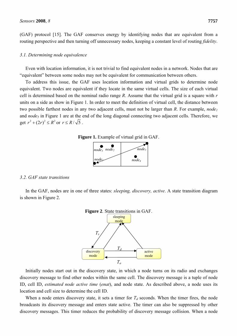
To address this issue, the GAF uses location information and virtual grids to determine node
equivalent. Two nodes are equivalent if they locate in the same virtual cells. The size of each virtual
cell is determined based on the nominal radio range R. Assume that the virtual grid is a square with r
units on a side as show in Figure 1. In order to meet the definition of virtual cell, the distance between
two possible farthest nodes in any two adjacent cells, must not be larger than R. For example, node1
and node5 in Figure 1 are at the end of the long diagonal connecting two adjacent cells. Therefore, we
get 2 2 2(2 )r r R or / 5r R .
Figure 1. Example of virtual grid in GAF.
3.2. GAF state transitions
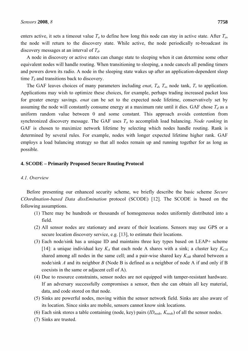
In the GAF, nodes are in one of three states: sleeping, discovery, active. A state transition diagram
is shown in Figure 2.
Figure 2. State transitions in GAF.
Initially nodes start out in the discovery state, in which a node turns on its radio and exchanges
discovery message to find other nodes within the same cell. The discovery message is a tuple of node
ID, cell ID, estimated node active time (enat), and node state. As described above, a node uses its
location and cell size to determine the cell ID.
When a node enters discovery state, it sets a timer for Td seconds. When the timer fires, the node
broadcasts its discovery message and enters state active. The timer can also be suppressed by other
discovery messages. This timer reduces the probability of discovery message collision. When a node
node1
node2 node3
node4
node5
sleeping mode
discovery mode
active mode
Ts
Td
Ta
Sensors 2008, 8
7758
enters active, it sets a timeout value Ta to define how long this node can stay in active state. After Ta,
the node will return to the discovery state. While active, the node periodically re-broadcast its
discovery messages at an interval of Td.
A node in discovery or active states can change state to sleeping when it can determine some other
equivalent nodes will handle routing. When transitioning to sleeping, a node cancels all pending timers
and powers down its radio. A node in the sleeping state wakes up after an application-dependent sleep
time TS and transitions back to discovery.
The GAF leaves choices of many parameters including enat, Td, Ta, node tank, Ts to application.
Applications may wish to optimize these choices, for example, perhaps trading increased packet loss
for greater energy savings. enat can be set to the expected node lifetime, conservatively set by
assuming the node will constantly consume energy at a maximum rate until it dies. GAF chose Td as a
uniform random value between 0 and some constant. This approach avoids contention from
synchronized discovery message. The GAF uses Ta to accomplish load balancing. Node ranking in
GAF is chosen to maximize network lifetime by selecting which nodes handle routing. Rank is
determined by several rules. For example, nodes with longer expected lifetime higher rank. GAF
employs a load balancing strategy so that all nodes remain up and running together for as long as
possible.
4. SCODE – Primarily Proposed Secure Routing Protocol
4.1. Overview
Before presenting our enhanced security scheme, we briefly describe the basic scheme Secure
COordination-based Data dissEmination protocol (SCODE) [12]. The SCODE is based on the
following assumptions.
(1) There may be hundreds or thousands of homogeneous nodes uniformly distributed into a
field.
(2) All sensor nodes are stationary and aware of their locations. Sensors may use GPS or a
secure location discovery service, e.g. [13], to estimate their locations.
(3) Each node/sink has a unique ID and maintains three key types based on LEAP+ scheme
[14]: a unique individual key KA that each node A shares with a sink; a cluster key KCH
shared among all nodes in the same cell; and a pair-wise shared key KAB shared between a
node/sink A and its neighbor B (Node B is defined as a neighbor of node A if and only if B
coexists in the same or adjacent cell of A).
(4) Due to resource constraints, sensor nodes are not equipped with tamper-resistant hardware.
If an adversary successfully compromises a sensor, then she can obtain all key material,
data, and code stored on that node.
(5) Sinks are powerful nodes, moving within the sensor network field. Sinks are also aware of
its location. Since sinks are mobile, sensors cannot know sink locations.
(6) Each sink stores a table containing (node, key) pairs (IDnode, Knode) of all the sensor nodes.
(7) Sinks are trusted.
Sensors 2008, 8
7759
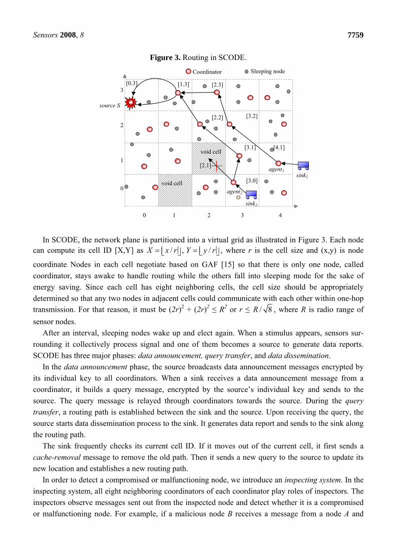
Figure 3. Routing in SCODE.
In SCODE, the network plane is partitioned into a virtual grid as illustrated in Figure 3. Each node can compute its cell ID [X,Y] as / , /X x r Y y r , where r is the cell size and (x,y) is node
coordinate. Nodes in each cell negotiate based on GAF [15] so that there is only one node, called
coordinator, stays awake to handle routing while the others fall into sleeping mode for the sake of
energy saving. Since each cell has eight neighboring cells, the cell size should be appropriately
determined so that any two nodes in adjacent cells could communicate with each other within one-hop
transmission. For that reason, it must be (2r)2 + (2r)2 ≤ R2 or r ≤ / 8R , where R is radio range of
sensor nodes.
After an interval, sleeping nodes wake up and elect again. When a stimulus appears, sensors sur-
rounding it collectively process signal and one of them becomes a source to generate data reports.
SCODE has three major phases: data announcement, query transfer, and data dissemination.
In the data announcement phase, the source broadcasts data announcement messages encrypted by
its individual key to all coordinators. When a sink receives a data announcement message from a
coordinator, it builds a query message, encrypted by the source’s individual key and sends to the
source. The query message is relayed through coordinators towards the source. During the query
transfer, a routing path is established between the sink and the source. Upon receiving the query, the
source starts data dissemination process to the sink. It generates data report and sends to the sink along
the routing path.
The sink frequently checks its current cell ID. If it moves out of the current cell, it first sends a
cache-removal message to remove the old path. Then it sends a new query to the source to update its
new location and establishes a new routing path.
In order to detect a compromised or malfunctioning node, we introduce an inspecting system. In the
inspecting system, all eight neighboring coordinators of each coordinator play roles of inspectors. The
inspectors observe messages sent out from the inspected node and detect whether it is a compromised
or malfunctioning node. For example, if a malicious node B receives a message from a node A and
source S
sink1
agent2
sink2
void cell
void cell
0 1 2 3 4
3 2 1 0
agent1
[4.1]
[3.0]
[3.1]
[3.2]
[2.3]
[2.2]
[1.3] [0.3]
[2.1]
Coordinator Sleeping node
Sensors 2008, 8
7760
attempts to modify it before forwarding to C, the common inspectors of A and B will detect the change
because they also receive the same messages sent out from A and B, so that they know the message
originated from B is not the same as the original message sent out from A.
Analysis and simulation results in [12] have shown that SCODE is much more energy-efficient than
existing approaches such as TTDD [17] and DD [18] while it always delivers 90% of packets to the
mobile sinks successfully. More importantly, SCODE is secure against common attacks in sensor
network routing mentioned in Section 2: spoofed, altered, or replayed routing information, selective
forwarding, sinkhole, Sybil, wormhole, and HELLO flood (unidirectional link) attacks. Though
SCODE is dominant over existing routing protocols, it still has a number of limitations, as pointed out
in Section 1.
5. SCODEplus: Enhanced Secure Routing and Key Management Scheme
5.1. Hexagonal Network Deployment
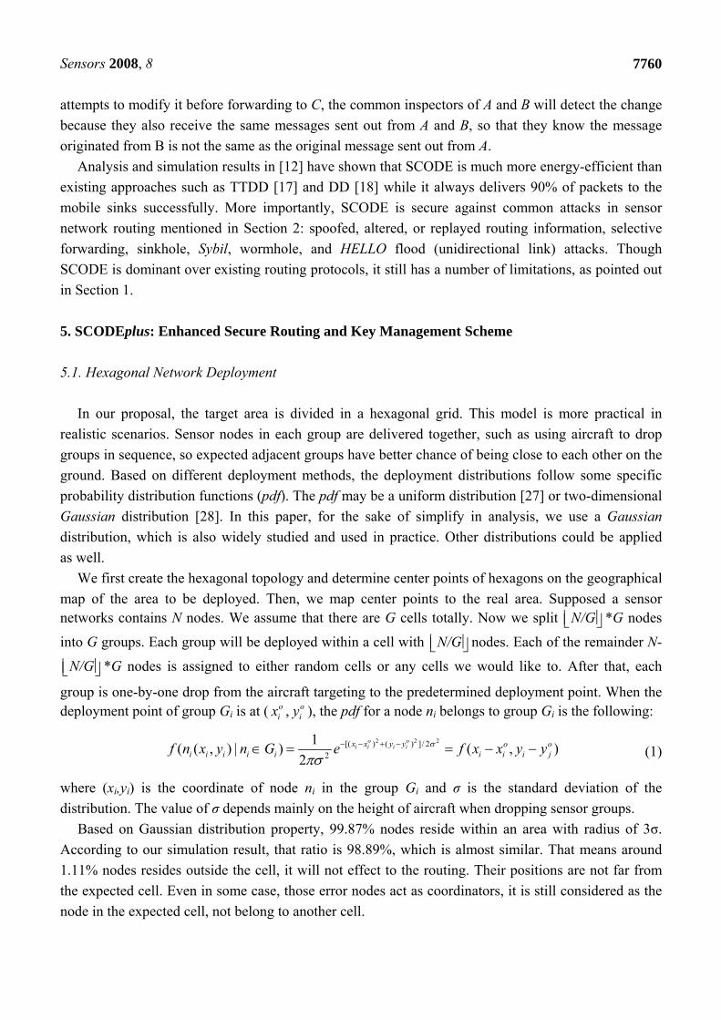
In our proposal, the target area is divided in a hexagonal grid. This model is more practical in
realistic scenarios. Sensor nodes in each group are delivered together, such as using aircraft to drop
groups in sequence, so expected adjacent groups have better chance of being close to each other on the
ground. Based on different deployment methods, the deployment distributions follow some specific
probability distribution functions (pdf). The pdf may be a uniform distribution [27] or two-dimensional
Gaussian distribution [28]. In this paper, for the sake of simplify in analysis, we use a Gaussian
distribution, which is also widely studied and used in practice. Other distributions could be applied
as well.
We first create the hexagonal topology and determine center points of hexagons on the geographical
map of the area to be deployed. Then, we map center points to the real area. Supposed a sensor networks contains N nodes. We assume that there are G cells totally. Now we split N/G *G nodes
into G groups. Each group will be deployed within a cell with N/G nodes. Each of the remainder N-
N/G *G nodes is assigned to either random cells or any cells we would like to. After that, each
group is one-by-one drop from the aircraft targeting to the predetermined deployment point. When the deployment point of group Gi is at ( o
ix , oiy ), the pdf for a node ni belongs to group Gi is the following:
2 2 2[( ) ( ) ]/ 22
1( ( , ) | ) ( , )
2
o oi i i ix x y y o o
i i i i i i i i jf n x y n G e f x x y y
(1)
where (xi,yi) is the coordinate of node ni in the group Gi and σ is the standard deviation of the
distribution. The value of σ depends mainly on the height of aircraft when dropping sensor groups.
Based on Gaussian distribution property, 99.87% nodes reside within an area with radius of 3σ.
According to our simulation result, that ratio is 98.89%, which is almost similar. That means around
1.11% nodes resides outside the cell, it will not effect to the routing. Their positions are not far from
the expected cell. Even in some case, those error nodes act as coordinators, it is still considered as the
node in the expected cell, not belong to another cell.
Sensors 2008, 8
7761
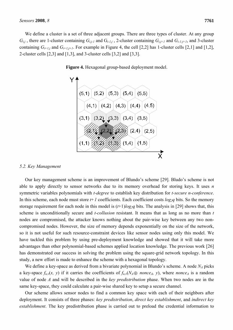
We define a cluster is a set of three adjacent groups. There are three types of cluster. At any group
Gi,j , there are 1-cluster containing Gi,j-1 and Gi-1,j , 2-cluster containing Gi,j+1 and Gi-1;j+1, and 3-cluster
containing Gi+1,j and Gi+1,j+1. For example in Figure 4, the cell [2,2] has 1-cluster cells [2,1] and [1,2],
2-cluster cells [2,3] and [1,3], and 3-cluster cells [3,2] and [3,3].
Figure 4. Hexagonal group-based deployment model.
5.2. Key Management
Our key management scheme is an improvement of Blundo’s scheme [29]. Bludo’s scheme is not
able to apply directly to sensor networks due to its memory overhead for storing keys. It uses n
symmetric variables polynomials with t-degree to establish key distribution for t-secure n-conference.
In this scheme, each node must store t+1 coefficients. Each coefficient costs log2q bits. So the memory
storage requirement for each node in this model is (t+1)log2q bits. The analysis in [29] shows that, this
scheme is unconditionally secure and t-collusion resistant. It means that as long as no more than t
nodes are compromised, the attacker knows nothing about the pair-wise key between any two non-
compromised nodes. However, the size of memory depends exponentially on the size of the network,
so it is not useful for such resource-constraint devices like sensor nodes using only this model. We
have tackled this problem by using pre-deployment knowledge and showed that it will take more
advantages than other polynomial-based schemes applied location knowledge. The previous work [26]
has demonstrated our success in solving the problem using the square-grid network topology. In this
study, a new effort is made to enhance the scheme with a hexagonal topology.
We define a key-space as derived from a bivariate polynomial in Blundo’s scheme. A node NA picks
a key-space fu,v(x, y) if it carries the coefficients of fu,v(NA nonceA, y), where nonceA is a random
value of node A and will be described in the key predistribution phase. When two nodes are in the
same key-space, they could calculate a pair-wise shared key to setup a secure channel.
Our scheme allows sensor nodes to find a common key space with each of their neighbors after
deployment. It consists of three phases: key predistribution, direct key establishment, and indirect key
establishment. The key predistribution phase is carried out to preload the credential information to
Sensors 2008, 8
7762
each sensor node before deployment. After setting up, two sensor nodes can establish a direct key
between them if they share at least a common key-space, otherwise, they could agree on an indirect
key according to the indirect key establishment phase.
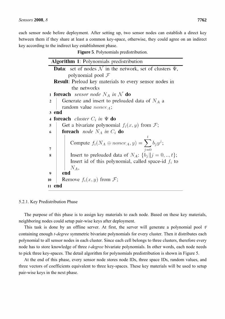
Figure 5. Polynomials predistribution.
5.2.1. Key Predistribution Phase
The purpose of this phase is to assign key materials to each node. Based on these key materials,
neighboring nodes could setup pair-wise keys after deployment. This task is done by an offline server. At first, the server will generate a polynomial pool F
containing enough t-degree symmetric bivariate polynomials for every cluster. Then it distributes each
polynomial to all sensor nodes in each cluster. Since each cell belongs to three clusters, therefore every
node has to store knowledge of three t-degree bivariate polynomials. In other words, each node needs
to pick three key-spaces. The detail algorithm for polynomials predistribution is shown in Figure 5.
At the end of this phase, every sensor node stores node IDs, three space IDs, random values, and
three vectors of coefficients equivalent to three key-spaces. These key materials will be used to setup
pair-wise keys in the next phase.
Sensors 2008, 8
7763
5.2.2. Direct Key Establish Phase
After deployment, every sensor node discovers the sharing key-space with its neighbors. Assume
that node NA with three space IDs fi, fj, fk needs to discover shared key-space with its neighbors. It
broadcasts a 1-hop discovery message Key-Space Discovery Message (KSDM) containing the
following information:
, , ( ), ( ), ( )A A i A j A k AN nounce H f nounce H f nounce H f nounce
where H is the hashing function and is the XOR operation.
When a neighbor of A, say B, receives this message, it finds out that it could share three, one or no
common key-space with A. Similarly, node A also receives B’s KSDM message and finds out common
key-spaces. If the sharing is at least one common key-space, the pair-wise key between B and A is
calculated at B as follows:
( , )BA B B A AK f N nounce N nounce (2)
After getting KBA, node B deletes value nonceA from its memory. The process of computing pair-
wise key at A is similar. Because of the symmetric property of bivariate polynomials, KAB = KBA. After
this phase, every node stores a list of pair-wise keys with its neighbors, beside the key-space
information and a random value in previous phase.
5.2.3. Indirect Key Establishment Phase
In case there is no common key-space between two neighboring nodes, it is needed to establish a
path key through one or more intermediate nodes. Our solution for this problem is as follows.
After the direct key establishment phase, every node A knows a set of secure neighboring nodes,
denoted as SA. Node A wants to establish a pair-wise shared key with its neighbor B, but B and A do
not share any key-space. In this situation, A generates a session key, called KS, and find a node say C
in SA that have the same group ID with node B or neighboring group ID of group containing node B.
Node A then sends a message containing KS encrypted by key KAC to node C. In turn, node C sends to
B a session key through a secure channel protected by the key KCB. The key KS then is used as pair-
wise shared key between two nodes A and B.
After above three phases, every node stores a table containing neighbor IDs and pair-wise shared
keys equivalently. The existence of key materials allows sensor networks to be able to add new nodes
for replacement later.
5.2.4. Establishing/Revoking Keys of New/Existing Sensors
To add a new sensor, the key setup server only needs to predistribute the related polynomial shares
to the new node, similar to predistribution phase. Since the size of key-space is limited, the more
sensors are added, the lower the security in that cell becomes.
The revocation method is also straightforward. Each sensor node only needs to store a black list IDs
of compromised sensors that share at least one bivariate polynomial with itself. If there are more than t
Sensors 2008, 8
7764
compromised nodes sharing the same polynomial, the non-compromised nodes that have this
polynomial will remove this polynomial and all related compromised nodes.
5.3. Secure Data Dissemination Scheme to Mobile Sinks
In this section, we present SCODEplus, a significantly enhanced version of the SCODE [12].
Different from the previous version, the routing algorithm in SCODEplus does not require locations of
sensor nodes. Each node knows their own group ID (cell ID) prior to the deployment. SCODEplus also
has three phases: data announcement, query transfer, and data dissemination. Those phases are similar
to that of the SCODE except the routing algorithm in query transfer phase. The previous routing
algorithm is based on square-grid structure. In this version, the routing algorithm is based on the
hexagonal network topology which provides more straight routing path between a source and a sink.
On the other hand, thank to our enhanced deployment model, the new routing algorithm can eliminate
the void cell problem of the previous scheme.
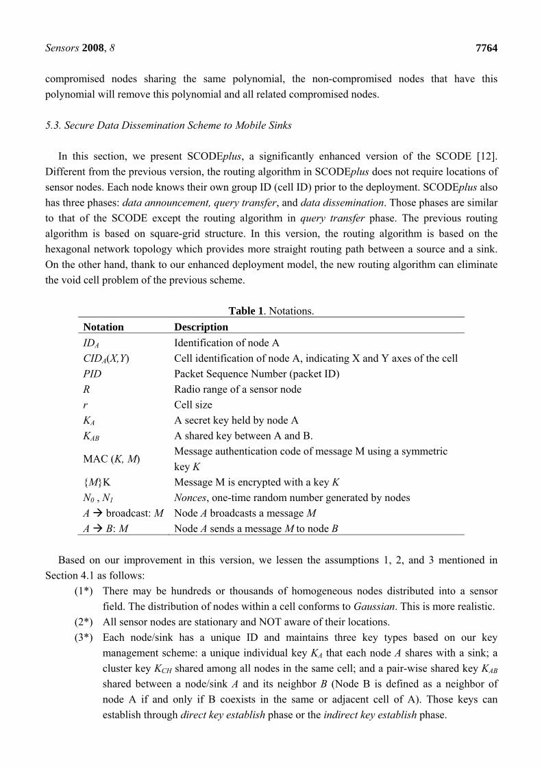
Table 1. Notations.
Based on our improvement in this version, we lessen the assumptions 1, 2, and 3 mentioned in
Section 4.1 as follows:
(1*) There may be hundreds or thousands of homogeneous nodes distributed into a sensor
field. The distribution of nodes within a cell conforms to Gaussian. This is more realistic.
(2*) All sensor nodes are stationary and NOT aware of their locations.
(3*) Each node/sink has a unique ID and maintains three key types based on our key
management scheme: a unique individual key KA that each node A shares with a sink; a
cluster key KCH shared among all nodes in the same cell; and a pair-wise shared key KAB
shared between a node/sink A and its neighbor B (Node B is defined as a neighbor of
node A if and only if B coexists in the same or adjacent cell of A). Those keys can
establish through direct key establish phase or the indirect key establish phase.
Notation Description
IDA Identification of node A
CIDA(X,Y) Cell identification of node A, indicating X and Y axes of the cell
PID Packet Sequence Number (packet ID)
R Radio range of a sensor node
r Cell size
KA A secret key held by node A
KAB A shared key between A and B.
MAC (K, M) Message authentication code of message M using a symmetric
key K
{M}K Message M is encrypted with a key K
N0 , N1 Nonces, one-time random number generated by nodes
A broadcast: M Node A broadcasts a message M
A B: M Node A sends a message M to node B
Sensors 2008, 8
7765
Table 1 provides the notation description which will be used in the paper.
5.3.1 Secure Neighboring Discovery
After deployment, each node A broadcasts a HELLO message in order to discover its neighborhoods.
This message is encrypted by A's cluster key KCH:
A → broadcast: {IDA | CIDA | N0}KCH
Each receiving node B decrypts the message and checks if it is a neighbor of A. If yes, it replies to A
node ID and cell ID along with a nonce value N0 encrypted by the pair-wise shared key KAB.
B → A: {IDB | CIDB | N0+1}KBA
Receiving node A decrypts the message using the pair-wise shared key. It then checks if the nonce
N0 is the one it has broadcasted. If it is, A accepts B as a neighbor and updates its neighborhood table.
The above two-way handshake protocol can avoid (or defend against) the unidirectional link
problems (or attacks) [16]. For example, if an attacker uses node A which is a more powerful node
such as a laptop with longer transmission range than B, then A can send a message to B directly, but B
cannot send a message to A within one-hop. However, node B still thinks that A is a one-hop
neighboring node and various problems may arise. For example, B tries to packets to A, since A is out
of B’s communication range, the packets will be dropped.
5.3.2. Three Main Phases.
(a) Phase 1: Secure Data Announcement:
When a stimulus is detected, a source S propagates a Data-Announcement (DA) message to all
coordinators using a flooding mechanism. The message contains source ID, cell ID and a MAC:
S broadcast: PID | IDS | CIDS |{DA}KS | MAC (KS, PID | IDS | CIDS | {DA}KS)
Every coordinator stores a few piece of information for the route discovery, including the
information of the stimulus and its cell ID. Since the coordinator role might be changed every time,
cell ID is the best solution for nodes to know the target it should relay the query to. In order to avoid
indefinite storing of data-announcement messages in each coordinator, the source attaches a timeout
parameter in each message. Within the timeout interval, if the coordinator has not received any
further data-announcement message, it removes the information of the stimulus and the source
location to free the cache.
(b) Phase 2: Secure Query Transfer and Route Discovery
Receiving a data-announcement message, a sink looks up in its {(IDnode, Knode)} table, finds the key
KS shared with the source, and uses it to decrypt the message. It then constructs a query message
using KS and sends back to the source via coordinators as follows:
o The sink first send message to its agent. The agent is a coordinator within the same cell. If the
sink locates outside of the network (not belong to any cell), then the agent would be the
coordinator in the closest cell.
Sensors 2008, 8
7766
Sink → Agent: PID | CIDThis| CIDNext | IDS | CIDS | IDSink | { QUERY }KS | MAC (KSinkAgent,
PID | CIDThis| CIDNext ) | MAC (KS, IDS | CIDS | IDSink | {QUERY }KS )
where CIDThis is cell ID of the agent, and CIDNext is cell ID of the next cell (in this case CIDThis
= CIDSink, and CIDNext = CIDAgent). The source key KS is used to encrypt the query content. It is
also used to build a MAC of IDS, CIDS, and IDSink in order to provide data authentication and
data integrity of the information sent from the sink. The pair-wise shared key KSinkAgent is used
to build a MAC of PID, CIDThis, and CIDNext in order to provide data authentication and data
integrity of the packet sent from the current node.
o The agent computes next cell ID (which is the closest cell to the destination) towards the
source, and then forwards the packet to it.
Agent Nextcell: PID | CIDThis| CIDNext | IDS | CIDS | IDSink | { QUERY }KS | MAC
(KAgentNextl, PID | CIDThis| CIDNext ) | MAC (KS, IDS | CIDS | IDSink | { QUERY } KS )
o Receiving coordinator checks whether its cell ID is the same as CIDNext in the message. If yes,
it computes next cell ID, and relays the message to it. Each node maintains a routing table
which stores the departure cell ID, the destination cell ID, the uplink cell ID (which it receives
the message) and the downlink cell ID (which is next cell ID CIDNext).
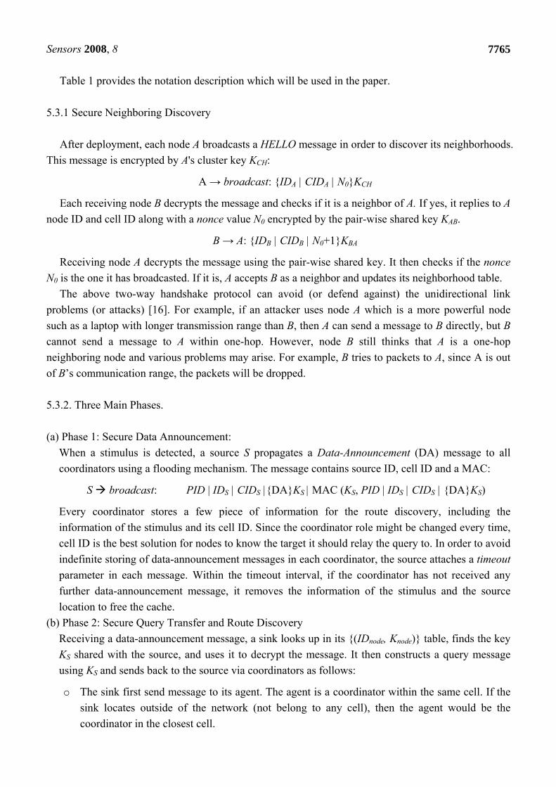
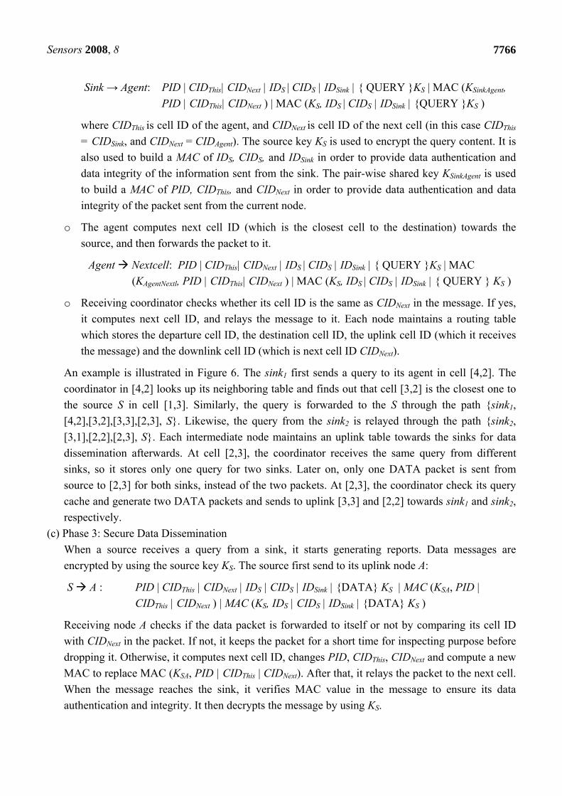
An example is illustrated in Figure 6. The sink1 first sends a query to its agent in cell [4,2]. The
coordinator in [4,2] looks up its neighboring table and finds out that cell [3,2] is the closest one to
the source S in cell [1,3]. Similarly, the query is forwarded to the S through the path {sink1,
[4,2],[3,2],[3,3],[2,3], S}. Likewise, the query from the sink2 is relayed through the path {sink2,
[3,1],[2,2],[2,3], S}. Each intermediate node maintains an uplink table towards the sinks for data
dissemination afterwards. At cell [2,3], the coordinator receives the same query from different
sinks, so it stores only one query for two sinks. Later on, only one DATA packet is sent from
source to [2,3] for both sinks, instead of the two packets. At [2,3], the coordinator check its query
cache and generate two DATA packets and sends to uplink [3,3] and [2,2] towards sink1 and sink2,
respectively.
(c) Phase 3: Secure Data Dissemination
When a source receives a query from a sink, it starts generating reports. Data messages are
encrypted by using the source key KS. The source first send to its uplink node A:
S A : PID | CIDThis | CIDNext | IDS | CIDS | IDSink | {DATA} KS | MAC (KSA, PID |
CIDThis | CIDNext ) | MAC (KS, IDS | CIDS | IDSink | {DATA} KS )
Receiving node A checks if the data packet is forwarded to itself or not by comparing its cell ID
with CIDNext in the packet. If not, it keeps the packet for a short time for inspecting purpose before
dropping it. Otherwise, it computes next cell ID, changes PID, CIDThis, CIDNext and compute a new
MAC to replace MAC (KSA, PID | CIDThis | CIDNext). After that, it relays the packet to the next cell.
When the message reaches the sink, it verifies MAC value in the message to ensure its data
authentication and integrity. It then decrypts the message by using KS.
Sensors 2008, 8
7767
Figure 6. An example of routing in SCODEplus.
5.3.3. Sink Mobility Management
Periodically, the sink checks the distance to the agent’s cell. If it recognizes that it no longer
reaches that cell within the sensor transmission range, the sink has to compute new cell ID and selects
a coordinator in that cell as a new agent. Then, the sink re-sends a query to the source to establish a
new data dissemination route by using the same mechanism described in the phase 2. By re-sending
queries only when the sink moves out of transmission range, SCODEplus significantly reduces
communication overhead compared with other approaches. Hence, collision and energy consumption
are reduced. Also, the number of loss data packet is decreased.
5.3.4. Coordination Election
As aforementioned, the proposed scheme is based on the GAF to establish a coordination network.
During the discovery phase, a node with the highest ranking will stay awake and play a role of a
coordinator while the others fall into sleeping mode. The node ranking is determined by an
application-dependent ranking procedure (it can be an arbitrary ordering of nodes to decide which
nodes would be active, or it can be selected to optimize overall network lifetime). In GAF, a node with
a longer expected lifetime is assigned a higher rank. This rule put nodes with longer expected lifetime
into use first. However, this is very vulnerable. An adversary can use a compromised node to advertise
the highest rank so that this node can be active all the time.
Practically, it is very hard (perhaps not possible) to absolutely defend against node compromise
attacks for GAF. Therefore, we modify the discovery process and the ranking rule of GAF in order to
reduce the risk without lessening its advantages. A coordinator is orderly selected according to node
0 1 2 3 4
3
2
1
0
source S
sink2
sink1
[3,1]
[2,2]
[2,3] [1,3] [3,3]
[4,2]
Coordinator Sleeping node
[3,2]
Agent2
Agent1
Sensors 2008, 8
7768
ID at each discovery round. For example, there are m nodes {ID1, ID2,…, IDm} (ID1 < ID2 < … < IDm)
in a certain cell, if node IDi is a coordinator at the current round, then IDi+1 would be a coordinator at
the next round; if i = m then “i + 1” would be 1. By doing this way, the adversary cannot make her
node active all the time at will. The compromised node is active only if it is a coordinator at the given
round. On the other hand, our enhancement reduces communication overhead compared with GAF
since nodes do not need to broadcast discovery messages.
Once a new coordinator is elected, the old coordinator forwards all current routing operations to the
new coordinator before it falls into the sleeping mode. That includes routing packets (if the transition
occurs during the routing operation), the routing caching table containing uplink and downlink nodes,
etc. The information is encrypted by their pairwise shared key. By doing this, it will not effect to the
existing dissemination flows.
5.4 Inspecting System
One of the most security concerns in sensor networks is node compromise. Due to resource
limitation, sensor nodes are not equipped with any tamper-resistant hardware. Once a node is
compromised, the adversary can extract all information stored in that node including all key materials.
Then the adversary can use this node to perform various types of attacks to the networks. Defending
against node compromise in routing is a non-trivial task.
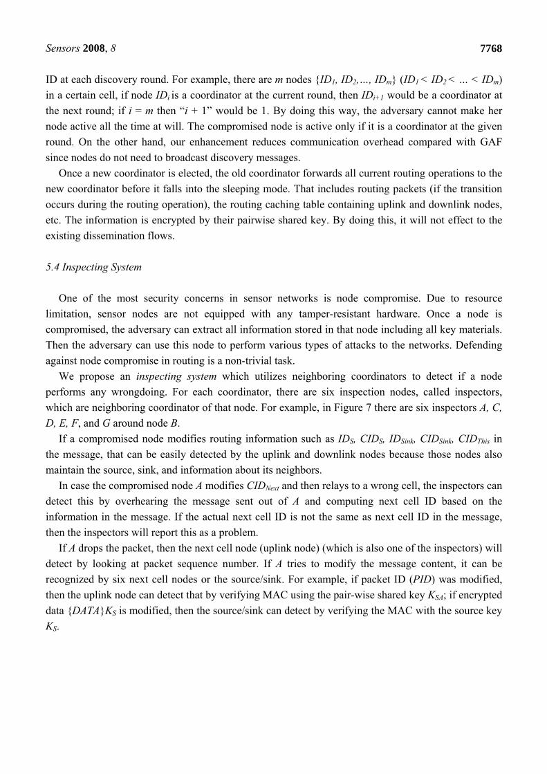
We propose an inspecting system which utilizes neighboring coordinators to detect if a node
performs any wrongdoing. For each coordinator, there are six inspection nodes, called inspectors,
which are neighboring coordinator of that node. For example, in Figure 7 there are six inspectors A, C,
D, E, F, and G around node B.
If a compromised node modifies routing information such as IDS, CIDS, IDSink, CIDSink, CIDThis in
the message, that can be easily detected by the uplink and downlink nodes because those nodes also
maintain the source, sink, and information about its neighbors.
In case the compromised node A modifies CIDNext and then relays to a wrong cell, the inspectors can
detect this by overhearing the message sent out of A and computing next cell ID based on the
information in the message. If the actual next cell ID is not the same as next cell ID in the message,
then the inspectors will report this as a problem.
If A drops the packet, then the next cell node (uplink node) (which is also one of the inspectors) will
detect by looking at packet sequence number. If A tries to modify the message content, it can be
recognized by six next cell nodes or the source/sink. For example, if packet ID (PID) was modified,
then the uplink node can detect that by verifying MAC using the pair-wise shared key KSA; if encrypted
data {DATA}KS is modified, then the source/sink can detect by verifying the MAC with the source key
KS.
Sensors 2008, 8
7769
Figure 7. Inspecting System.
Once the compromised node is detected, the inspectors alert to other coordinators and eliminate that
node from participating in the routing process. Coordinators consider that cell a void cell and establish
another route by finding a round path. For example in Figure 7, the coordinator A is legitimate node,
and B is a compromised node. Node C and G are common inspectors of A and B, so they can receive
the message sent out from A and B and can detect if B is doing something wrong. When C and G detect
B as a compromised node, they send an alert message to the neighboring coordinator of B including A,
D, E, and F. The alert message sent from C will go through C→D→E→F→G→A→C. The alert
message sent out from G will go through G→F→E→D→C→A→G. This duplicated alert message
makes sure that the compromised node is detected by two inspectors. The alert message is encrypted
by the pairwise key between the sender and the receiver. For example, G sends an alert message to F:
G → F: IDG, CIDG, IDB, CIDB, MAC(KGF, IDG, CIDG, IDB, CIDB) (3)
where IDG, CIDG is node ID and cell ID of the inspector which detects compromised node, and IDB,
CIDB is the node ID and cell ID of the compromised node.
6. Analysis
In the previous version [12], we have argued that the proposed routing protocol is secure against
common attacks mentioned in Section 2: spoofed, altered, or replayed routing information [9], [16],
selective forwarding [16], sinkhole [16], Sybil [10], wormhole [11], HELLO flood (unidirectional link)
attacks [16]. In this section, we are focusing on security of inspecting system, security and efficiency
of the enhanced key management scheme.
6.1. Inspecting System Security
An adversary can target inspection nodes in two ways. Firstly, by deploying several nodes to report
fake inspection information to the network. Secondly, by compromising a number of nodes to fool the
entire network. We shall discuss those vulnerabilities in the following sections.
B A
C D
E
F G
Alert message from G
Ordinary packet
Alert message from C
Compromised node
Legitimate node
Sensors 2008, 8
7770
6.1.1. The adversary deploys some nodes to report wrong inspecting information
Once a coordinator detects a compromised node, it sends an alert message to the neighboring
coordinators of that node using a pairwise key. For example in equation (3), node G detects B as a
compromised node, it sends an alert message to node F using pairwise key KGF. These keys are
unknown to the adversary. So even she deploys some nodes and they send the wrong information, it
can be easily detected by verifying MAC value in the alert message.
6.1.2. The adversary compromises some inspectors to fool the entire network
Inspecting system is based on mutual inspection. This means that every coordinator could become
an inspector, and vice versa. If the adversary compromises an inspector, then that inspector can be
detected by other legitimate nodes. Therefore, the adversary cannot cheat the entire network unless she
compromises all the nodes, which is not feasible.
6.2. Network Connectivity
In this section, we discuss network connectivity including local connectivity and global
connectivity. Local connectivity is the probability a node could connect with neighbor nodes within its
transmission range. Global connectivity is the ratio of the number of sensor nodes forming the largest
isolated connected component in the final key graph G to the size of the whole network. In node
compromise attacks, adversaries usually launch node compromise attacks in order to eavesdrop secure
channels in the network, or using key materials revealed from compromised nodes to perform node
replication attacks. In this regard, we discuss whether nodes compromised attacks could be used for
eavesdropping or not. We denote ),( ji nnA as in , jn are neighboring, ),( ji nnB as the two nodes share a pairwise key. The
local connectivity could be calculated as.
)),((
)),(),(()),(|),((
ji
jijijijilocal nnAP
nnAnnBPnnAnnBPP
Probability that a node ii Gn is a neighbor of node ),( jjj yxn is the integral of pdf )( inf over
the circle around node jn with radius R
RyxyxG
ijjj
jji
dxdyyxnfyxnP),(),,(,
)),(()),((
Because jn distribute in group jG following (1) the probability that ii Gn is a neighbor of jj Gn :
jG
jjjjjiji dxdyyxnfyxnPGGnnAP )),(()),((),||),((
Hence,
),||),(()()()),(( jijiG G
jjiiji GGnnAPGnPGnPnnAPi j
Denoted )( iGS is set of neighboring groups of iG we have
Sensors 2008, 8
7771
( )
( ( , ) ( , )) ( ) ( ) ( ( , ) || , )i j i
i j i j i i j j i j i jG G S G
P B n n A n n P n G P n G P A n n G G
Because a sensor node is chosen in a given group with an equal probability, we have the local
connectivity can be calculated as
i j
i ij
G Gjiji
G GSGjiji
local GGnnAP
GGnnAP
P),||),((
),||),(()(
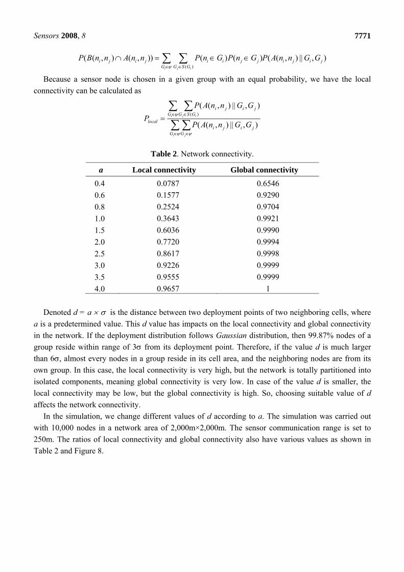
Table 2. Network connectivity.
a Local connectivity Global connectivity
0.4 0.0787 0.6546
0.6 0.1577 0.9290
0.8 0.2524 0.9704
1.0 0.3643 0.9921
1.5 0.6036 0.9990
2.0 0.7720 0.9994
2.5 0.8617 0.9998
3.0 0.9226 0.9999
3.5 0.9555 0.9999
4.0 0.9657 1
Denoted d = a is the distance between two deployment points of two neighboring cells, where
a is a predetermined value. This d value has impacts on the local connectivity and global connectivity
in the network. If the deployment distribution follows Gaussian distribution, then 99.87% nodes of a
group reside within range of 3 from its deployment point. Therefore, if the value d is much larger
than 6, almost every nodes in a group reside in its cell area, and the neighboring nodes are from its
own group. In this case, the local connectivity is very high, but the network is totally partitioned into
isolated components, meaning global connectivity is very low. In case of the value d is smaller, the
local connectivity may be low, but the global connectivity is high. So, choosing suitable value of d
affects the network connectivity.
In the simulation, we change different values of d according to a. The simulation was carried out
with 10,000 nodes in a network area of 2,000m×2,000m. The sensor communication range is set to
250m. The ratios of local connectivity and global connectivity also have various values as shown in
Table 2 and Figure 8.
Sensors 2008, 8
7772
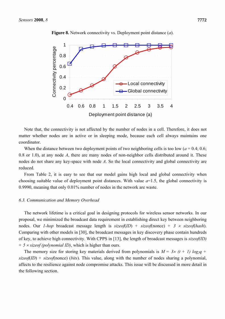
Figure 8. Network connectivity vs. Deployment point distance (a).
0
0.2
0.4
0.6
0.8
1
0.4 0.6 0.8 1 1.5 2 2.5 3 3.5 4
Deployment point distance (a)
Co
nn
ect
ivity
pe
rce
nta
ge
Local connectivity
Global connectivity
Note that, the connectivity is not affected by the number of nodes in a cell. Therefore, it does not
matter whether nodes are in active or in sleeping mode, because each cell always maintains one
coordinator.
When the distance between two deployment points of two neighboring cells is too low (a = 0.4; 0.6;
0.8 or 1.0), at any node A, there are many nodes of non-neighbor cells distributed around it. These
nodes do not share any key-space with node A. So the local connectivity and global connectivity are
reduced.
From Table 2, it is easy to see that our model gains high local and global connectivity when
choosing suitable value of deployment point distances. With value a=1.5, the global connectivity is
0.9990, meaning that only 0.01% number of nodes in the network are waste.
6.3. Communication and Memory Overhead
The network lifetime is a critical goal in designing protocols for wireless sensor networks. In our
proposal, we minimized the broadcast data requirement in establishing direct key between neighboring
nodes. Our 1-hop broadcast message length is sizeof(ID) + sizeof(nonce) + 3 sizeof(hash).
Comparing with other models in [30], the broadcast messages in key discovery phase contain hundreds
of key, to achieve high connectivity. With CPPS in [13], the length of broadcast messages is sizeof(ID)
+ 5 sizeof (polynomial ID), which is higher than ours.
The memory size for storing key materials derived from polynomials is M = 3 (t + 1) log2q +
sizeof(ID) + sizeof(nonce) (bits). This value, along with the number of nodes sharing a polynomial,
affects to the resilience against node compromise attacks. This issue will be discussed in more detail in
the following section.
Sensors 2008, 8
7773
6.4. Resilience against Node Compromise Attacks on Key Management
The proposed model has two stages that could be a target for node capture attacks. The first stage is
a period between the distribution of sensor nodes to the target field, and establishment of pair-wise
key. The second one is after broadcasting discovery messages and forming a connected pair-wise key
network. The properties of two stages lead to different security levels.
In the first stage, adversaries can capture enough sensor nodes in a cluster to interpolate
polynomials, and then eavesdrops KSDM messages to get nonce values. The number of sufficient
compromised sensor nodes depends on the polynomial degree that is the memory for storing key
materials. In this manner, attackers could generate all pair-wise keys in the cluster. So the security in
this stage needs some consideration. But we need to remember that the time of this stage is quite short
right after deployment, so a chance for an adversary to launch attacks is not highly possible.
In the second stage, from (2) we can see that each pair-wise key depends not only on key-space
information but also on random values associated with each node. Suppose that a node A is
compromised and an adversary could get all information stored inside the A’s memory. In this case,
she could only get pair-wise keys between A and its neighbors, and a fraction of polynomial f(NA, y).
Even if she compromises a sufficiently large number of nodes like A, then still it is not possible for an
adversary to expose pair-wise key between non-compromised nodes B and C. This is due to the fact
that the adversary does not have the information about the random numbers stored on the non-
compromised nodes. So, compared with other schemes such as [26]-[30], our scheme has not been
affected by node capture attacks on the links between non-compromised nodes.
7. Performance Evaluation
We have evaluated SCODEplus performance and compared with the SCODE [12], TTDD [17], and
DD [18]. The evaluation was carried out by simulation on SENSE simulator (Sensor Network
Simulator and Emulator) [20].
7.1. Simulation Model
The network comprises 400 nodes randomly deployed in a 2,000 m × 2,000 m area. We use the
same energy model in ns-2.1b8a [21] that requires 0.66W, 0.359W and 0.035W for transmitting,
receiving and idling, respectively. We set the power consumption rates of RC5 according to [22][23]
for encryption, MAC computation, and random number generation are 0.65W, 0.48W, and 0.36W,
respectively. As analyzed in [19][24], we set the time consumption for encrypting 64 bits with RC5
0.26 ms, generating 64 pseudorandom bits takes 0.26 ms, and computing a 4- byte MAC requires 0.13
ms. The simulation uses MAC 802.11 Distributed Coordination Function (DCF) and nominal
transmission range of each node is 250m. Two-ray ground [25] is used as the radio propagation model.
Each data packet has 64 bytes, query packets and the others are 36 bytes long. Additional bytes for
MACs and nonce values are also put into each message. The default number of sinks is 8 moving with
speed 10m/s according to random way-point model. Two sources generate different packets at an
average interval of 1 second. Summary of parameters and defined values are shown in Table 3.
Sensors 2008, 8
7774
Table 3. Simulation parameters and defined values.
Simulation Parameters Value
N (total nodes) 400 nodes
A (network size) 2,000 m × 2,000 m
Transmission 0.66W
Reception 0.359W
Idle 0.035W
RC5 encryption of 64 bits 0.26 ms
Pseudorandom number generation 0.26 ms
4-byte MAC generation 0.13 ms
R 250 m
Data packet size 64 bytes
Other packet size 32 bytes
Number of mobile sinks 8
Default speed of mobile sinks 10 m/s
Data generation interval 1 second
7.2. Simulation Results
Since SCODEplus is targeted to multiple and mobile sinks in sensor networks, we study the impact
of the number of sinks, sink’s speed, and the density of the network. We measure the energy
consumption, average delay (average response time to users), and success ratio (total number of
packets has been delivered successfully).
7.2.1. Impact of Sink Number
As many users may simultaneously access the sensor network, it is important to consider the impact
of the sink number. For the sensor network area of 2,000 m×2,000 m, we set the number of sink
varying from 1 to 8. Each sink moves with the maximum speed 10 m/s and a 5-second pause time. The
number of total nodes and the number of sources are not changed.
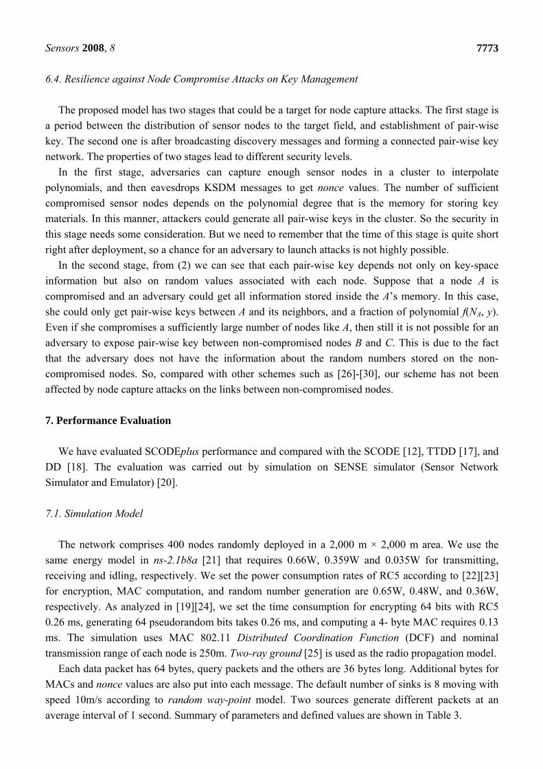
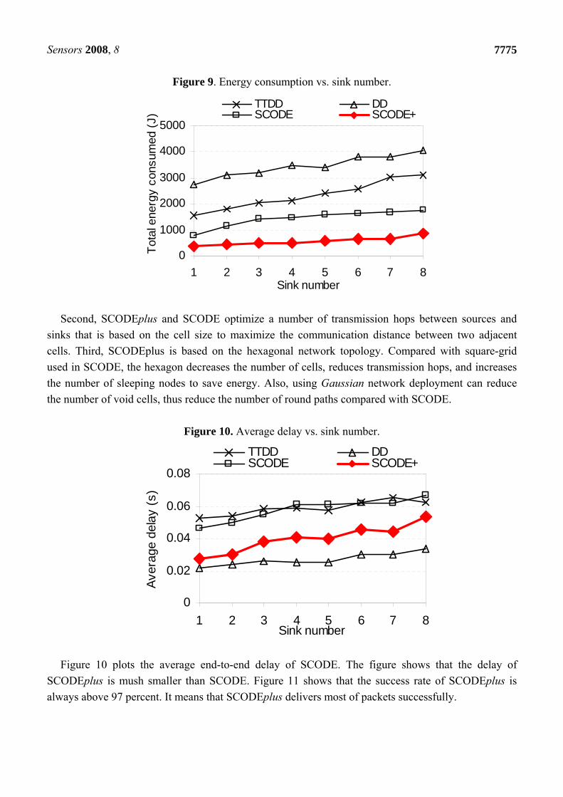
Figure 9 shows total energy consumption of SCODE as the number of sinks varies from 1 to 8. It
demonstrates that SCODEplus is more energy efficient than SCODE, TTDD, and DD. This is because
of three reasons. First, SCODEplus and SCODE are based on a coordination network, so that nodes in
each cell negotiate among themselves to turn off its radio to significantly reduce energy consumption.
Meanwhile, TTDD and DD must turn on all nodes to participate in routing.
Sensors 2008, 8
7775
Figure 9. Energy consumption vs. sink number.
0
1000
2000
3000
4000
5000
1 2 3 4 5 6 7 8Sink number
Tot
al e
nerg
y co
nsum
ed (
J)
TTDD DDSCODE SCODE+
Second, SCODEplus and SCODE optimize a number of transmission hops between sources and
sinks that is based on the cell size to maximize the communication distance between two adjacent
cells. Third, SCODEplus is based on the hexagonal network topology. Compared with square-grid
used in SCODE, the hexagon decreases the number of cells, reduces transmission hops, and increases
the number of sleeping nodes to save energy. Also, using Gaussian network deployment can reduce
the number of void cells, thus reduce the number of round paths compared with SCODE.
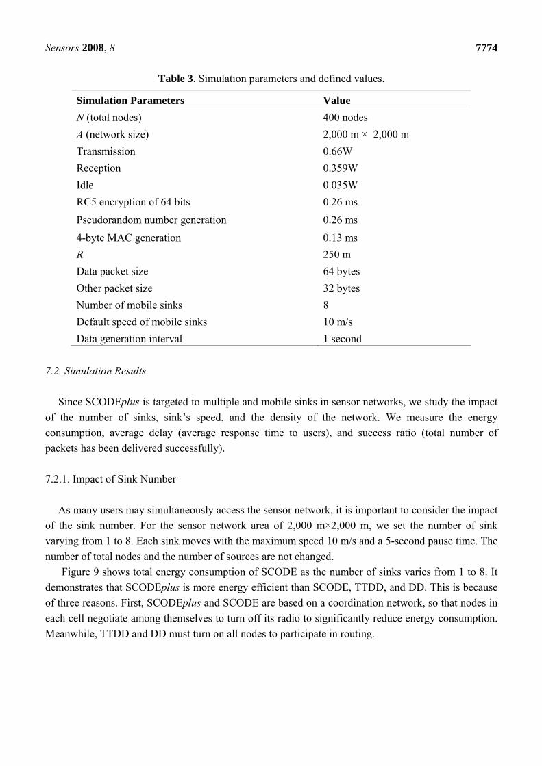
Figure 10. Average delay vs. sink number.
0
0.02
0.04
0.06
0.08
1 2 3 4 5 6 7 8Sink number
Ave
rage
del
ay (
s)
TTDD DDSCODE SCODE+
Figure 10 plots the average end-to-end delay of SCODE. The figure shows that the delay of
SCODEplus is mush smaller than SCODE. Figure 11 shows that the success rate of SCODEplus is
always above 97 percent. It means that SCODEplus delivers most of packets successfully.
Sensors 2008, 8
7776
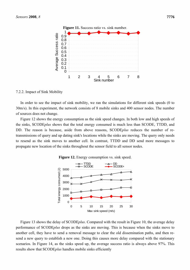
Figure 11. Success ratio vs. sink number.
00.10.20.30.40.50.60.70.80.9
1
1 2 3 4 5 6 7 8Sink number
Ave
rage
Suc
cess
rat
io
7.2.2. Impact of Sink Mobility
In order to see the impact of sink mobility, we ran the simulations for different sink speeds (0 to
30m/s). In this experiment, the network consists of 8 mobile sinks and 400 sensor nodes. The number
of sources does not change.
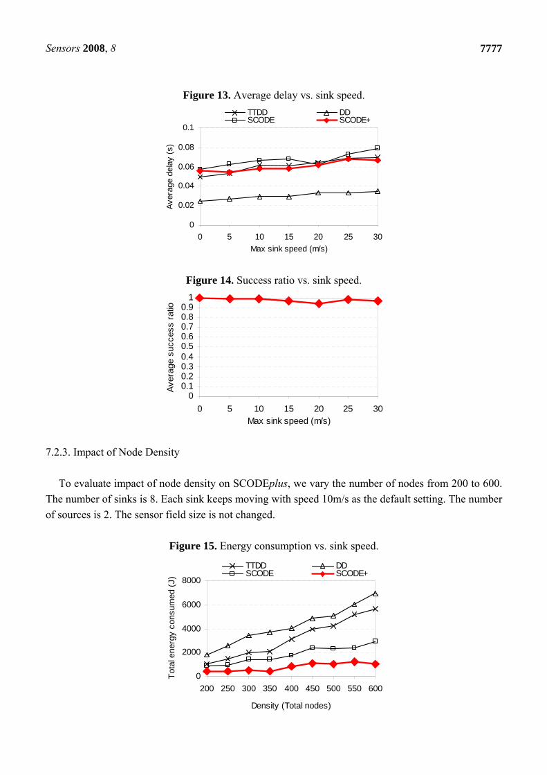
Figure 12 shows the energy consumption as the sink speed changes. In both low and high speeds of
the sinks, SCODEplus shows that the total energy consumed is much less than SCODE, TTDD, and
DD. The reason is because, aside from above reasons, SCODEplus reduces the number of re-
transmissions of query and up dating sink's locations while the sinks are moving. The query only needs
to resend as the sink moves to another cell. In contrast, TTDD and DD send more messages to
propagate new location of the sinks throughout the sensor field to all sensor nodes.
Figure 12. Energy consumption vs. sink speed.
0
1000
2000
3000
4000
5000
0 5 10 15 20 25 30
Max sink speed (m/s)
Tot
al e
nerg
y co
nsum
ed (
J)
TTDD DDSCODE SCODE+
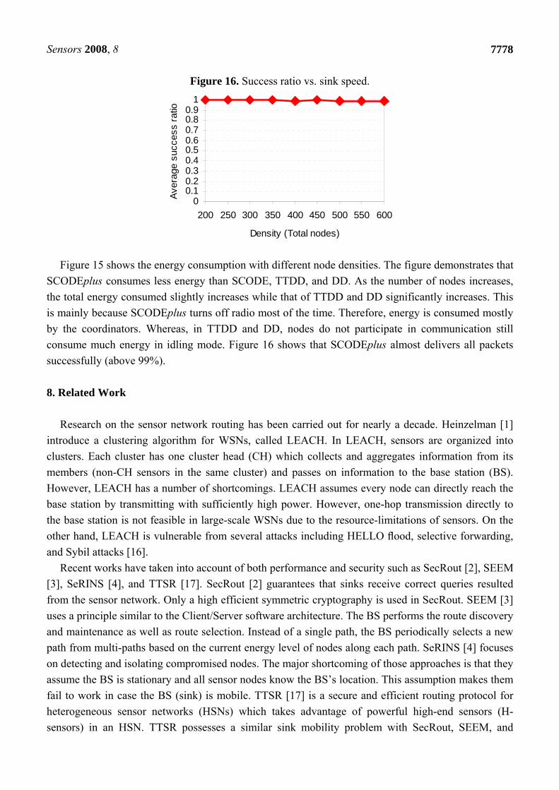
Figure 13 shows the delay of SCODEplus. Compared with the result in Figure 10, the average delay
performance of SCODEplus drops as the sinks are moving. This is because when the sinks move to
another cell, they have to send a removal message to clear the old dissemination paths, and then re-
send a new query to establish a new one. Doing this causes more delay compared with the stationary
scenarios. In Figure 14, as the sinks speed up, the average success ratio is always above 97%. This
results show that SCODEplus handles mobile sinks efficiently
Sensors 2008, 8
7777
Figure 13. Average delay vs. sink speed.
0
0.02
0.04
0.06
0.08
0.1
0 5 10 15 20 25 30
Max sink speed (m/s)
Ave
rage
del
ay (
s)
TTDD DDSCODE SCODE+
Figure 14. Success ratio vs. sink speed.
00.10.20.30.40.50.60.70.80.9
1
0 5 10 15 20 25 30Max sink speed (m/s)
Ave
rage
suc
cess
rat
io
7.2.3. Impact of Node Density
To evaluate impact of node density on SCODEplus, we vary the number of nodes from 200 to 600.
The number of sinks is 8. Each sink keeps moving with speed 10m/s as the default setting. The number
of sources is 2. The sensor field size is not changed.
Figure 15. Energy consumption vs. sink speed.
0
2000
4000
6000
8000
200 250 300 350 400 450 500 550 600
Density (Total nodes)
Tot
al e
nerg
y co
nsum
ed (
J)
TTDD DDSCODE SCODE+
Sensors 2008, 8
7778
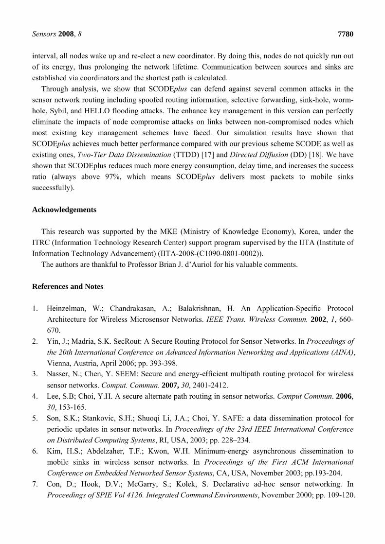
Figure 16. Success ratio vs. sink speed.
00.10.20.30.40.50.60.70.80.9
1
200 250 300 350 400 450 500 550 600
Density (Total nodes)
Ave
rage
suc
cess
rat
io
Figure 15 shows the energy consumption with different node densities. The figure demonstrates that
SCODEplus consumes less energy than SCODE, TTDD, and DD. As the number of nodes increases,
the total energy consumed slightly increases while that of TTDD and DD significantly increases. This
is mainly because SCODEplus turns off radio most of the time. Therefore, energy is consumed mostly
by the coordinators. Whereas, in TTDD and DD, nodes do not participate in communication still
consume much energy in idling mode. Figure 16 shows that SCODEplus almost delivers all packets
successfully (above 99%).
8. Related Work
Research on the sensor network routing has been carried out for nearly a decade. Heinzelman [1]
introduce a clustering algorithm for WSNs, called LEACH. In LEACH, sensors are organized into
clusters. Each cluster has one cluster head (CH) which collects and aggregates information from its
members (non-CH sensors in the same cluster) and passes on information to the base station (BS).
However, LEACH has a number of shortcomings. LEACH assumes every node can directly reach the
base station by transmitting with sufficiently high power. However, one-hop transmission directly to
the base station is not feasible in large-scale WSNs due to the resource-limitations of sensors. On the
other hand, LEACH is vulnerable from several attacks including HELLO flood, selective forwarding,
and Sybil attacks [16].
Recent works have taken into account of both performance and security such as SecRout [2], SEEM
[3], SeRINS [4], and TTSR [17]. SecRout [2] guarantees that sinks receive correct queries resulted
from the sensor network. Only a high efficient symmetric cryptography is used in SecRout. SEEM [3]
uses a principle similar to the Client/Server software architecture. The BS performs the route discovery
and maintenance as well as route selection. Instead of a single path, the BS periodically selects a new
path from multi-paths based on the current energy level of nodes along each path. SeRINS [4] focuses
on detecting and isolating compromised nodes. The major shortcoming of those approaches is that they
assume the BS is stationary and all sensor nodes know the BS’s location. This assumption makes them
fail to work in case the BS (sink) is mobile. TTSR [17] is a secure and efficient routing protocol for
heterogeneous sensor networks (HSNs) which takes advantage of powerful high-end sensors (H-
sensors) in an HSN. TTSR possesses a similar sink mobility problem with SecRout, SEEM, and

Sensors 2008, 8
7779
SeRINS. On the other hand, TTSR is only suitable for HSNs with sufficient powerful sensor nodes,
not large-scale homogeneous WSNs. Besides, relying only on some particular nodes makes them prone
to deplete there energy sooner or later. Using fixed coordinators makes attackers easy to choose ’right’
nodes to compromise.
There are a number of routing protocols aiming to support mobile sinks in WSNs [5][6][7][17][18].
Declarative Routing Protocol [7], and Directed Diffusion (DD) [18] suggest that each mobile sink
needs to continuously propagate its location information throughout the sensor field, so that all sensor
nodes get updated with the direction of sending future data reports. However, frequent location update
from multiple sinks leads to both increased collisions in wireless transmissions and rapid power
consumption of the sensor’s limited battery supply. SAFE [5] uses flooding that is geographically
limited to forward the query to nodes along the direction of the source. Considering the large number
of nodes in WSNs, the network-wide flooding may introduce considerable traffic. SEAD [6] considers
the distance and the packet traffic rate among nodes to create a near-optimal dissemination. SEAD
strikes a balance between end-to-end delay and power consumption that favors power saving over
delay minimization. It is therefore only suitable for applications with a less strict delay requirement.
TTDD [17] exploits local flood within a local cell of a virtual grid which sources build proactively.
However, it does not optimize the path from the source to the sinks. When a source communicates with
a sink, the restriction of grid structure may multiply the length of a straight-line path by 2 . Also,
TTDD frequently renews the entire path to the sinks. It therefore increases energy consumption and
connection loss ratio. Those multi-hop routing protocols face many security problems from spoofed,
altered, or replayed routing information [9][16], selective forwarding [16], sinkhole [16], Sybil [10],
wormhole [11], and HELLO flood (unidirectional link) attacks [16].
Our protocol overcomes those shortcomings by considering security and routing protocol at the
design time. The scheme is based on GAF, along with a hexagonal deployment model to achieve better
security and efficiency. It securely disseminates 97% data packets to the mobile sinks successfully and
even more efficiently than non-secure approaches like TTDD and DD.
9. Conclusions
In this paper we have presented a first, novel energy-efficient secure routing and key management
scheme for mobile sinks in sensor networks, namely SCODEplus. It is a significant enhancement of
our previous study, Secure COodination-based Data dissEmination protocol for mobile sinks
(SCODE) [12]. Besides several improvements, this study was recognized by a careful consideration of
security (key management scheme) during the design time. Those not only enhance security but also
increase efficiency of the proposed scheme.
SCODEplus takes advantages of a coordination network based on GAF and a hexagonal
deployment model to apply an energy-efficient secure routing and key management scheme for mobile
sinks. In SCODEplus, the sensor network plane is partitioned into a hexagonal structure. An efficient
key management based on Blundo’s scheme is applied to reduce memory requirements and increase
the security level. The cell size is optimal to increase network connectivity and reduce the number of
transmission hops. Sensor nodes in each cell negotiate among each other so that only one node, called
coordinator, stays awake and the others fall into sleeping mode for the sake of energy. After an
Sensors 2008, 8
7780
interval, all nodes wake up and re-elect a new coordinator. By doing this, nodes do not quickly run out
of its energy, thus prolonging the network lifetime. Communication between sources and sinks are
established via coordinators and the shortest path is calculated.
Through analysis, we show that SCODEplus can defend against several common attacks in the
sensor network routing including spoofed routing information, selective forwarding, sink-hole, worm-
hole, Sybil, and HELLO flooding attacks. The enhance key management in this version can perfectly
eliminate the impacts of node compromise attacks on links between non-compromised nodes which
most existing key management schemes have faced. Our simulation results have shown that
SCODEplus achieves much better performance compared with our previous scheme SCODE as well as
existing ones, Two-Tier Data Dissemination (TTDD) [17] and Directed Diffusion (DD) [18]. We have
shown that SCODEplus reduces much more energy consumption, delay time, and increases the success
ratio (always above 97%, which means SCODEplus delivers most packets to mobile sinks
successfully).
Acknowledgements
This research was supported by the MKE (Ministry of Knowledge Economy), Korea, under the
ITRC (Information Technology Research Center) support program supervised by the IITA (Institute of
Information Technology Advancement) (IITA-2008-(C1090-0801-0002)).
The authors are thankful to Professor Brian J. d’Auriol for his valuable comments.
References and Notes
1. Heinzelman, W.; Chandrakasan, A.; Balakrishnan, H. An Application-Specific Protocol
Architecture for Wireless Microsensor Networks. IEEE Trans. Wireless Commun. 2002, 1, 660-
670.
2. Yin, J.; Madria, S.K. SecRout: A Secure Routing Protocol for Sensor Networks. In Proceedings of
the 20th International Conference on Advanced Information Networking and Applications (AINA),
Vienna, Austria, April 2006; pp. 393-398. 3. Nasser, N.; Chen, Y. SEEM: Secure and energy-efficient multipath routing protocol for wireless
sensor networks. Comput. Commun. 2007, 30, 2401-2412.
4. Lee, S.B; Choi, Y.H. A secure alternate path routing in sensor networks. Comput Commun. 2006,
30, 153-165.
5. Son, S.K.; Stankovic, S.H.; Shuoqi Li, J.A.; Choi, Y. SAFE: a data dissemination protocol for
periodic updates in sensor networks. In Proceedings of the 23rd IEEE International Conference
on Distributed Computing Systems, RI, USA, 2003; pp. 228–234.
6. Kim, H.S.; Abdelzaher, T.F.; Kwon, W.H. Minimum-energy asynchronous dissemination to
mobile sinks in wireless sensor networks. In Proceedings of the First ACM International
Conference on Embedded Networked Sensor Systems, CA, USA, November 2003; pp.193-204.
7. Con, D.; Hook, D.V.; McGarry, S.; Kolek, S. Declarative ad-hoc sensor networking. In
Proceedings of SPIE Vol 4126. Integrated Command Environments, November 2000; pp. 109-120.
Sensors 2008, 8
7781
8. Ye, F., Zhong, G.; Lu, S.; Zhang, L. GRAdient Broadcast: A Robust Data Delivery Protocol for
Large Scale Sensor Networks. Wireless Netw. 2005, 11, 285-298.
9. Wood, A.D.; Stankovic, J.A. Denial of service in sensor networks. Computer 2002, 35, 54–62.
10. Douceur, J.R. The Sybil attack. In Proceedings of 1st International Workshop on Peer-to-Peer
Systems, MA, USA, Mar, 2002; pp. 251–260.
11. Hu, Y.-C.; Perrig, A.; Johnson, D.B. Wormhole detection in wireless ad hoc networks. Technical
Report TR01384, Department of Computer Science, Rice University, June 2002.
12. Hung L.X.; Lee S.Y.; Lee Y.-K; Lee H.J. SCODE: A Secure Coordination-based Data
Dissemination to Mobile Sinks in Wireless Sensor Networks. IEICE Trans. Commun. 2009, E92-
B(01).
13. Lazos, L.; Poovendran, R. SeRLoc: Secure range-independent localization for wireless sensor
networks. In Proceedings of ACM Workshop on Wireless Security, PA, USA, October 2004; pp.
21–30.
14. Zhu, S.; Setia, S.; Jajodia, S. LEAP+: Efficient Security Mechanisms for Large-Scale Distributed
Sensor Networks. ACM Trans. Sens. Netw. 2006, 2, 500–528.
15. Xu, Y.; Heidemannn, J.; Estrin, D. Geography informed energy conservation for ad hoc routing.
In Proceedings of the Seventh Annual ACM/IEEE International Conference on Mobile Computing
and Networking (MobiCom 2001), Italy, July 2001; pp.70-84.
16. Karlof, C.; Wagner, D. Secure Routing in Wireless Sensor Networks: Attacks and
Countermeasures. In Proceedings of the First IEEE International Workshop on Sensor Network
Protocols and Applications (SPNA), AK, USA, May 2003; pp. 113-127.
17. Ye, F.; Luo, H.; Cheng, J.; Lu, S.; Zhang, L. TTDD: A two-tier data dissemination model for
large-scale wireless sensor networks. Wirel. Netw. 2005, 11, 161 -175.
18. Intanagonwiwat, C.; Govindan, R.; Estrin, D.; Heidemann, J.; Silva, F. Directed Diffusion for
wireless sensor networking. IEEE/ACM Trans. Netw. 2003, 11, 2-16.
19. Karlof, C. ; Sastry, N.; Dagner, D. TinySec: A Link Layer Security Architecture for Wireless
Sensor Networks. In Proceedings of the 2nd International Conference on Embedded Networked
Sensor Systems (SenSys04), Baltimore, Maryland, November 2004; pp. 162-175.
20. Chen, G.; Branch, J.; Pflug, M.J.; Zhu, L. and Szymanski, B. SENSE: A Sensor Network
Simulator, Advances in Pervasive Computing and Networking; Springer: New York, NY, 2004;
pp. 249-269.
21. NS-2; http://www.isi.edu/nsnam/ns/.
22. Xue, Q.; Ganz, A. Runtime security composition for sensor networks. In Proceedings of IEEE
Vehicular Technology Conference, FL, USA, October 2003; pp. 105–111.
23. Du, X.J.; Guizani, M.; Xiao, Y.; Chen, H.H. Two Tier Secure Routing Protocol for Heterogeneous
Sensor Networks. IEEE Trans. Wireless Commun. 2007, 6, 3395-3401.
24. Benenson, Z.; Freiling, F.C.; Hammerschmidt, E.; Lucks, S.; Pimenidis, L. Authenticated Query
Flooding in Sensor Networks. In Proceedings of the 4th annual IEEE International Conference
on Pervasive Computing and Communications Workshops, Pisa, Italy; pp. 38-49.
25. Rappaport, T.S. Wireless communications, Principles and Practice. Prentice Hall: New Jersey,
1996.
Sensors 2008, 8
7782
26. Canh, N.T.; Lee, Y.-K.; Lee, S.Y. HGKM - a group-based key management scheme for sensor
networks using deployment knowledge. In Proceedings of Sixth Annual Conference on
Communication Networks and Services Research (CNSR), Halifax, Nova Scotia, May 2008; pp.
544-551.
27. Liu, D.; Ning, P. Improving Key Predistribution with Deployment Knowledge in Static Sensor
Networks. ACM Trans. Sens. Netw. 2005, 1, 204–239.
28. Du, W.; Deng, J.; Han, Y.; Varshney, P. A Key Predistribution Scheme for Sensor Networks
Using Deployment Knowledge. IEEE Trans. Depend. Secure 2006, 3, 62–77.
29. Blundo, C.; Santis, A.D.; Herzberg, A.; Kutten, S.; Vaccaro, U.; Yung, M. Perfect-Secure Key
Distribution of Dynamic Conferences. In Proceedings of Advances in Cryptography,
BalatonfÜred, Hungary; pp. 471–486.
30. Chan, H.; Perrig, A.; Song, D. Random Key Predistribution Schemes for Sensor Networks, In
Proceedings of IEEE Symposium on Security and Privacy, CA, USA, May 2003; pp. 197–213.
31. Chen, B.; Jamieson, K.; Balakrishnan, H.; Morris, R. Span: An energy-efficient coordination
algorithm for topology maintenance in ad hoc wireless networks. Wireless Netw. 2002, 8, 481-494.
© 2008 by the authors; licensee Molecular Diversity Preservation International, Basel, Switzerland.
This article is an open-access article distributed under the terms and conditions of the Creative
Commons Attribution license (http://creativecommons.org/licenses/by/3.0/).