An Assessment of CFD/CSD Prediction State-of-the-ArtUsing the HART II International Workshop Data

Marilyn J. Smith∗ Joon W. Lim † Berend G. van der Wall ‡

Georgia Inst. of Tech. US Army AFDD-1 (AMRDEC) German Aerospace Center (DLR)Atlanta, GA, USA Moffett Field, CA, USA Braunschweig, Germany

James D. Baeder§ Robert T. Biedron¶ D. Douglas Boyd, Jr.‖

University of Maryland NASA Langley Research Center NASA Langley Research CenterCollege Park, MD, USA Hampton, VA, USA Hampton, VA, USA

Buvana Jayaraman∗∗ Sung N. Jung†† Byung-Young Min‡‡

Science & Technology Corp. Konkuk University Georgia Inst. of Tech.Moffett Field, CA, USA Seoul, South Korea Atlanta, GA, USA

Over the past decade, there have been significant advancements in the accuracy of rotor aeroelasticsimulations with the application of computational fluid dynamics methods coupled with computationalstructural dynamics codes (CFD/CSD). The HART II International Workshop database, which in-cludes descent operating conditions with strong blade-vortex interactions (BVI), provides a unique op-portunity to assess the ability of CFD/CSD to capture these physics. In addition to a baseline case withBVI, two additional cases with 3/rev higher harmonic blade root pitch control (HHC) are available forcomparison. The collaboration during the workshop permits assessment of structured, unstructured,and hybrid overset CFD/CSD methods from across the globe on the dynamics, aerodynamics, andwake structure. Evaluation of the plethora of CFD/CSD methods indicate that the most important nu-merical variables associated with most accurately capturing BVI are a two-equation or detached eddysimulation (DES)-based turbulence model and a sufficiently small time step. An appropriate trade-offbetween grid fidelity and spatial accuracy schemes also appears to be important for capturing BVIon the advancing rotor disk. Overall, the CFD/CSD methods generally fall within the same accuracy;cost-effective hybrid Navier-Stokes/Lagrangian wake methods tend to correlate less accurately with ex-periment and have larger data scatter than the full CFD/CSD methods for most parameters evaluated.The importance of modeling the fuselage is observed, and other requirements are discussed.

∗ corresponding author, Associate Professor, mari-lyn.smith@ae.gatech.edu

† Research Scientist, lim@merlin.arc.nasa.gov‡ Senior Scientist, berend.vanderwall@dlr.de§ Associate Professor, baeder@umd.edu¶ Senior Research Scientist, r.t.biedron@nasa.gov‖ Senior Research Engineer, d.d.boyd@nasa.gov∗∗Research Scientist, buvana.jayaraman@us.army.mil††Professor, snjung@konkuk.ac.kr‡‡Senior Research Scientist currently at the United

Technologies Research Center, minb@utrc.utc.comPresented at the American Helicopter Society 68th AnnualForum, Ft. Worth, TX, May 1–3, 2012. This is a work of theU.S. Government and is not subject to copyright protectionin the U.S.

This information product has been reviewed and approvedfor public release. The views expressed herein are those ofthe author and do not reflect the official policy or positionof the Department of the Army, Department of Defense,or the U.S. Government. Reference herein to any specificcommercial, private or public products, process, or serviceby trade name, trademark, manufacturer, or otherwise, doesnot constitute or imply its endorsement, recommendation,or favoring by the United States Government.

1

NOMENCLATURE

a∞ speed of sound, m/sc airfoil chord, mCmM2 section moment coefficient,

CmM2 = (dMc/4/dy)/(ρ∞a2∞c2/2)

CnM2 section force coefficient,CnM2 = (dL′/dy)/(ρ∞a2

∞c/2)CT thrust coefficient, CT = T/(ρ∞πΩ2R4)f ,g functiondL′/dy section lift, N/mdMc/4/dy section moment, Nm/mMh hover tip Mach number, Mh = ΩR/a∞

Mx rotor hub roll moment, NmMy rotor hub pitch moment, NmM∞ free-stream Mach number, M∞ =V∞/a∞

n integerNb number of bladesp∞ static air pressure, kPaP rotor power, kWr Pearson product moment coefficientra non-dimensional root cut-out radiusrtw non-dimensional zero twist radiusR rotor radius, ms standard deviation, variable unitst time, sT thrust, NT∞ air temperature, CV∞ air speed, m/sx,y,z chord, radial, normal coordinates,

respectively, mxel elastic deflection, mxhub Hub center distance to nozzle, myhub Hub position above centerline, mα angle of attack, degreesαS rotor shaft angle of attack, degrees∆αs wind tunnel interference angle, degreesφ mode shapeΘC lateral cyclic pitch angle, degreesΘS longitudinal cyclic pitch angle, degreesΘel elastic twist angle, degreesΘtw linear blade twist, degrees/RΘ75 collective pitch angle at 0.75R, degreesΘ3 HHC pitch angle at 3/rev, degreesµ advance ratio, µ =V∞cosαS/(ΩR)ρ∞ air density, kg/m3

σ rotor solidity, σ = Nbc/(πR2)ψ azimuth, ψ = Ωt, degreesψ3 phase of 3/rev HHC pitch angle, degreesΩ rotor rotational frequency, radians/s. mean

INTRODUCTION

During the past decade, an experimental data set developedvia a significant international collaboration has been ob-tained and extensively studied. This data set, known asthe HART II rotor data set, has provided a wealth of per-formance data (airloads and wake), as well as aeroacous-tics data for the development of aeroelastic and aeroacous-tic prediction methods. A subset of these data was openedto the public in 2005; and in conjunction with the releaseof these experimental data, a series of workshops (Ref. 1)have been held, first on a semi-annual and more recentlyon an annual basis. Active participants of the workshophave included researchers from the US government (AFDD,NASA-Ames and NASA-Langley, NIA); universities (PSU,UMD, GIT); Germany (DLR, Univ. of Stuttgart); France(Onera); England (Univ. of Glasgow); Japan (JAXA); andSouth Korea (KARI, Konkuk University). A plethora of dif-ferent computational investigations across the globe haveused these data to both validate new simulation methodsand to understand the physics of a rotor encountering bladevortex interactions (BVI).

These computational investigations have included thegamut of engineering assumptions included in comprehen-sive rotorcraft methods through computational fluid dynam-ics (CFD) coupled with computational structural dynamics(CSD) and computational aeroacoustics (CAA) methodolo-gies. Individual or small collaborative efforts have beenpublished and have resulted in advancements in the stateof the art regarding modeling issues and numerical meth-ods development. However, it has been difficult to as-sess the overall state of the art and best practices for allmajor (structured, unstructured, and hybrid) CFD/CSD ap-proaches given the differences in the assumptions and pre-sentation of the data in these works.

This effort gathers published and unpublished simula-tion results from the international team of experts shown inTable 1 who have been studying the HART II data set us-ing CFD/CSD coupled methodologies. This compendiumof results establishes simulation and modeling guidelines,provides a summary of state-of-the-art BVI CFD/CSD pre-dictions, and explores the use of higher harmonic control(HHC) to reduce or eliminate BVI. This paper also providesdirection for future experimental and simulation efforts,such as the international STAR collaboration. A compan-ion paper (Ref. 2) explores the same parameter and modelspace, but analyzes the ability of lower-fidelity aerodynam-ics (finite-state, prescribed and free wake models) to capturethe physics of the rotor.

HART II EXPERIMENT

In 2001, the second Higher-Harmonic Control Aeroacous-tic Rotor Test (HART II) was performed in the 8m ×

2

Table 1. Partners and CodesPartner Partner label CFD Code CSD Code

U.S. Army Aero-flightdynamics Dir. AFDD-1 OVERFLOW CAMRADIIU.S. Army Aero-flightdynamics Dir. AFDD-2 NSU3D-SAMARC RCASNASA-Langley NL-1 OVERFLOW CAMRADIINASA-Langley NL-2 FUN3D CAMRADIIGeorgia Institute of Technology GIT-1 FUN3D DYMORE4Georgia Institute of Technology GIT-2 GENCAS DYMORE2Konkuk University KU KFLOW CAMRADIIUniversity of Maryland UM TURNS UMARCGerman Aerospace Center DLR N/A S4

6m open-jet facility of the German-Dutch wind tunnel(DNW) in a cooperative American-French-German-Dutcheffort (Ref. 3). The model rotor consisted of a Mach- anddynamically-scaled BO105 rotor blade. Data available forcomparison include blade motion, sectional air loads, pres-sure distributions along the leading edge, tip vortex trajec-tories and flow fields, in addition to acoustic radiation. Im-portant variables that define the simulation conditions forthis experiment are summarized in Table 2.

A detailed description of the HART II data and how theywere measured will not be given in this paper, as this isavailable in the test documentation and has been reported innumerous papers and reports (Refs. 1, 3–7). The referencerotor condition in this work is the HART II Baseline case(BL).

Due to wind tunnel interference, the rotor thrust deflectsthe slip stream, reducing the effective angle of attack to ap-proximately α = 4.5. This condition results in descend-ing flight where strong blade-vortex interaction (BVI) oc-curs in the first quadrant (ψ ≈ 50) and the fourth quadrant(ψ ≈ 300) on the rotor disk where the vortex axis and theblade leading edge are approximately parallel to one an-other.

To evaluate the ability of higher harmonic control to re-duce or eliminate the BVI, HHC with 3/rev and a blade rootpitch control angle of Θ3 = 0.8 was applied at a phase ofψ3 = 300 to reduce BVI noise radiation (minimum noisecase, MN) and at ψ3 = 180 to reduce rotor vibrations (min-imum vibration case, MV). Both of these HHC cases1 il-lustrate the significant impact that HHC can have on BVI-related artifacts, such as noise and vibration.

This effort examines the following data from experimentacross the CFD/CSD simulations: tip blade motion com-pared to experiment, sectional aerodynamic loading (CnM2

1The MN and MV naming convention was adopted fromthe 1994 HART I test. However, the HHC control anglesfrom the HART I test are larger than the HHC control anglesin the HART II test.

and CmM2) at the 87% radial station, flap and lag bendingmoments at the 17% radial station, torsion moment at the33% radial station, lateral tip vortex positions at the ±70%radial station in the hub coordinate system, and global trimdata such as shaft angle, trim controls and targets. Giventhe length and complexity of this current effort, aeroacous-tic simulation evaluations are not included.

COMPUTATIONAL METHODOLOGIES

The computational methodologies applied in this effortconsisted of computational fluid dynamics modules (CFDmethods) coupled with computational structural dynam-ics modules (CSD) to provide aeroelastic simulations. Asnoted in Table 1, the methods applied were not exclusive toany one participant. Therefore, the methods are introducedby methodology name, rather than the participant name.

Computational Fluid Dynamics (CFD) Methods

The partners applied six different CFD codes in this anal-ysis, including four structured (OVERFLOW, TURNS,GENCAS, KFLOW) and two unstructured (FUN3D,NSU3D) methods. The Helios framework combined aCartesian background method (SAMARC) with the un-structured near-body solver (NSU3D). Two team membersapplied hybrid Navier-Stokes near-body solvers with free-wake farfield methods (GENCAS, TURNS/PWAM). Eachof these methods is briefly described, in particular the fea-tures which are pertinent to this effort.

FUN3D (Refs. 8, 9) solves the unsteady Navier-Stokesequations on unstructured grids, with several one- and two-equation turbulence models available to complete the sys-tem of equations. Inviscid fluxes are computed with second-order spatial accuracy by using one of several upwindschemes. Viscous fluxes are evaluated with a second-orderdiscretization that is equivalent to a Galerkin scheme ontetrahedral meshes. FUN3D is a node-centered code; so

3

Table 2. Summary of HART II Rotor TestCharacteristic Symbol Value

Rotor geometry:Rotor radius R 2 mBlade chord c 0.121 mNumber of blades Nb 4Rotor solidity σ 0.077Non-dim. root cutout ra 0.22Non-dim. zero twist radius rtw 0.75Blade linear twist Θtw -8 /RAirfoil (trailing edge tab) NACA23012

Wind tunnel data:Cross-section 8m ×6mAir pressure p∞ 100.97 kPaAir temperature T∞ 17.3 CAir density ρ∞ 1.2055 kg/m3

Speed of sound a∞ 341.7 m/sWind speed V∞ 32.9 m/sMach number M∞ 0.0963Hub center dist. to nozzle xhub/R 3.5Hub pos. up of centerline zhub/R 0.4575

Operational data (BL case):Rotational speed Ω 109.12 rad/sHover blade tip Mach no. Mh 0.639Rotor shaft angle of attack αS 5.3

Wind tunnel interference angle ∆αS -0.8

Advance ratio µ 0.151Rotor thrust T 3300 NThrust coefficient CT 0.00457Rotor loading coefficient CT/σ 0.0594Roll moment Mx 20 NmPitch moment My -20 NmRotor power P 18.3 kWCollective control at rtw Θ75 3.8

Lateral cyclic control ΘC 1.92

Longitudinal cyclic control ΘS -1.34

Mean steady el. tip twist Θel -1.09

the number of unknowns is directly related to the numberof nodes in the grid. The code supports ‘mixed-element’meshes in which the nodes may be connected into any com-bination of prisms, hexahedra, tetrahedra, and pyramids.Typical meshes use prisms near solid walls and tetrahe-dra outside of the boundary layer, with a limited numberof pyramids providing transition between the two regions.

The solver has a robust implicit time-advancementscheme and a variety of mesh-motion options, includingrigid, deforming, and overset meshes (Ref. 10). The time-advancement scheme makes use of an enhanced, second-order accurate backward difference scheme (Ref. 11) thatis formally second-order accurate but has a leading-order

error term that is roughly one half that of the standardsecond-order scheme. In addition, a temporal-error con-troller (Ref. 12) is used to help insure that a sufficient num-ber of subiterations are performed to drive the subitera-tion residual below the temporal error, thereby maintain-ing the design order of the scheme. For overset meshes,the DiRTlib (Ref. 13) and SUGGAR++ (Ref. 14) codes areused to facilitate communication between disparate zonesin the mesh.

General mesh motion and robust time advancement arecrucial for rotorcraft applications, where the flow is fun-damentally unsteady, and the flexible rotor blades undergolarge motions relative to the fuselage. O’Brien (Ref. 15)first applied the FUN3D solver to rotorcraft simulations,with the restriction of rigid blades in prescribed motion.Subsequent modifications (Ref. 16) resulted in a more gen-eral rotorcraft capability, with the ability to account foraeroelastic effects and trim via coupling with the Com-prehensive Analytical Model of Rotorcraft Aerodynamicsand Dynamics II (CAMRADII) code (Ref. 17). In sepa-rate efforts, Abras (Ref. 18) loosely coupled and Reveleset al. (Ref. 19) tightly coupled FUN3D with the DYMORECSD code (Ref. 20).

Loose coupling (applied in this effort) between FUN3Dand the CSD methods is implemented via the loosely cou-pled delta airloads strategy outlined in Ref. 21, and thus isappropriate to steady, level flight. The coupling is achievedvia file exchange or Python scripting, and either approach isgoverned by a shell script that orchestrates the execution ofthe codes and provides restart, post-processing, and archiv-ing functions. A typical coupled simulation proceeds as fol-lows. First, a trimmed CSD solution is obtained with theCSD internal aerodynamics model, typically with a simpleuniform or finite-state inflow. Blade displacements for onecomplete revolution are output by the CSD module for thefirst pass through FUN3D, where typically two completerevolutions are performed to remove large initial transients.FUN3D extracts airloads at selected stations along the rotorblades to obtain the airloads for one complete revolution.

Delta airloads from the previous coupling cycle are com-puted and passed to the CSD code, which then determinesa new trim solution and blade motions. The process is thenrepeated until convergence, although for subsequent cyclesFUN3D is run for only 2/Nb revolutions between couplingcycles (1/Nb revolution is a minimum; the extra 1/Nb revo-lution helps damp out transients during initial coupling cy-cles). This coupling strategy has not been examined foroptimality; however, it has proven to be a robust strategy(stable and convergent). The coupling process is deemed tohave converged when 1) trim control angles reported by theCSD code vary by less than 0.01 between coupling cycles,and 2) the thrust values obtained by integrating the sectionaldata provided by FUN3D and the corresponding data com-puted by the CSD code at the same sectional and azimuthal

4

locations, agree to within 0.1%. Fewer than 10 couplingcycles are usually required to meet these criteria.

GENCAS (Generic Numerical Compressible AirflowSolver) (Refs. 22, 23) is a generic Reynolds AveragedNavier-Stokes (RANS) solver including Hybrid Navier-Stokes/Free-wake method. In this hybrid method, only asingle blade is modeled with the RANS solver. The effectof other blades is accounted for by a bound vortex and tipvortices. The free-wake model consists of a tip vortex fromeach blade shed from the tip periodically with the maxi-mum bound vortex strength defined at the time at which itis shed. The effect of these tip vortices on the RANS solveris applied through outer surface boundary condition usingBiot-Savart law.

GENCAS is coupled with the CSD solver, DYMOREversion 2.0 (DYMORE2), and the delta airloads looselycoupled approach (Ref. 21) is applied to obtain the aeroe-lastic simulation. DYMORE runs with its own lifting linemodel as the first step, then the blade motion includingpitch control and elastic deformation from DYMORE is fedinto GENCAS. GENCAS interpolates the deformation dataincluding three linear and three angular deformations us-ing spline interpolation, as DYMORE2 is run at larger az-imuthal time steps than the GENCAS solver. The delta air-loads are then computed and provided to DYMORE.

Helios (Refs. 24, 25), under development by the U.S.Army through the CREATE program, is a multi-disciplinary computational platform. Helios includes soft-ware components responsible for near-body (NSU3D) andoff-body (SAMARC), domain connectivity (PUNDIT), ro-torcraft comprehensive analysis (RCAS or CAMRADII),mesh motion and deformation (MMM), a fluid-structureinterface module (RFSI) and a fluid-flight dynamics in-terface (FFDI) module. All these components are inter-faced together using a flexible and light-weight Python-based infrastructure called the Software Integration Frame-work (SIF). Figure 1 shows a schematic of the SIF. To pre-serve modularity, all data transfer between components oc-cur through the SIF and no component is allowed to “talk”directly to another component. The parallel execution ofthe SIF is accomplished using pyMPI.

Helios employs an innovative dual-mesh paradigm thatuses unstructured meshes in the near-body for ease of meshgeneration and Cartesian meshes in the off-body for betteraccuracy and efficiency. The two mesh types overlap eachother with data exchange between the two systems managedby a domain connectivity formulation. The unstructuredmeshes are body-conforming and are comprised of a mix oftetrahedrons, prisms and pyramids. The Cartesian meshesare managed by a block-structured mesh system, which hasthe ability to conform to the geometry and solution features.

Fig. 1. Python-based infrastructure in Helios

The near-body solver NSU3D uses a node-centeredfinite-volume scheme that is spatially second-order accu-rate. An edge-based data structure is used, which fa-cilitates flux computations on the edges of the median-dual control volume. Time-accurate computations employa second-order accurate backwards Euler algorithm withsubiterations applied in dual-time algorithm to converge thenon-linear problem at each time-step. The implicit solu-tion algorithm applies multigrid with line-Jacobi relaxationto smooth each grid level. The single-equation Spalart-Allmaras model is used to model turbulence.

The structured adaptive Cartesian code SAMARC isused for the off-body Cartesian grid. SAMARC solvesthe Euler equations using a fifth-order spatial discretizationand third-order Runge-Kutta time integration. The off-bodygrid has the ability to automatically adapt to the unsteadygeometry and solution features.

Both NSU3D and SAMARC run in parallel. PUNDITmanages overset domain connectivity on the partitionedgrid system. It automatically determines which grid andsolver apply in different regions of the flow field, computesthe interpolation operations between different grid systems,and manages the parallel exchange of data.

Rotorcraft structural dynamics and trim are solved us-ing a CSD method, currently either Rotorcraft Comprehen-sive Analysis System (RCAS) (Ref. 26) or CAMRADII(Ref. 17). At each coupling iteration the aerodynamicforces on the blade computed by CFD are passed to theCSD code. The CSD code computes the deflections basedon the CFD forces and passes the deflections back to CFDat some n/Nb intervals, where n is an integer (typically oneor two) and Nb is the number of rotor blades. This se-quence is repeated until the loads and deflections convergeto a periodic steady-state solution using the delta-airloadsapproach (Ref. 21).

KFLOW is a structured RANS solver capable of solv-ing time-accurate moving body problems by employinga Chimera overlapped grid system (Refs. 27, 28). Asecond-order accurate, dual-time stepping scheme, com-bined with a diagonalized alternating-directional implicit(DADI) method, is used for the temporal scheme. Forthe spatial discretization, a fifth-order weighted essentially

5

non-oscillatory (WENO) scheme is used for the inviscidfluxes, and the central difference scheme is adopted for theviscous fluxes.

The delta-airloads loose coupling approach (Ref. 21) hasbeen adopted to systematically couple the CAMRADII andKFLOW codes. Both the control trim angles and blade mo-tion data are computed from the CSD code, while KFLOWgenerates the CFD airloads acting on the blades. The deltaairloads between the two codes is calculated and fed into theCSD code to obtain updated blade motions and trim angles.This process is repeated until the airloads and trim valuesare generally within a tolerance of 0.1% between couplingiterations. Since the blade motion data from the CSD mod-ule are obtained at significantly larger time steps than thecorresponding CFD module, a fitting technique based onthe mode shapes and a Fourier series (Ref. 29) is employedto obtain sufficiently smooth curves to be interpolated andapplied in the CFD analysis.

OVERFLOW2 (Ref. 30) is a structured mesh methodol-ogy developed by NASA and has been extensively appliedto rotorcraft configurations, including CFD/CSD loose cou-pling (for example, Ref. 18, 21, 31). Spatial discretiza-tion formulations that span second- to sixth-order accuracyare available to resolve the inviscid terms and in conjunc-tion with several dissipation schemes. Turbulence simu-lation options include a large selection of RANS, hybridRANS-LES, and LES/VLES turbulence methods. In thiseffort, the Spalart-Allmaras (SA) and Spalart-Allmaras De-tached Eddy Simulation (SA-DES) models were appliedby AFDD-1 and NL-1 partners, respectively. The versionsof OVERFLOW applied in this effort are 2.2c (NL-1) and2.1ac (AFDD-1).

The aeroelastic behavior of rotors can be modeled usinga loosely- or tightly-coupled CFD/CSD strategy (Refs. 19,21, 32). The loosely coupled CFD/CSD approach (used inthis effort) applies the delta airloads technique (Ref. 21),which exchanges data between the CFD and CSD codes atregular intervals defined as integer multiples of the blade-rotor fraction of n/Nb. OVERFLOW has been coupled withthe CAMRADII (Ref. 17), RCAS (Ref. 26), and DYMORE(Ref. 20) CSD codes.

TURNS/PWAM (Transonic Unsteady Rotor Navier-Stokes) is a computational fluid dynamics solver capa-ble of solving unsteady aerodynamics flows. It appliesa second-order backward difference method using Lower-Upper Symmetric Gauss Seidel (LUSGS) (Refs. 33, 34)for time integration. Six Newton subiterations are used toremove factorization errors and recover time accuracy forunsteady computations (Ref. 35). The inviscid fluxes arecomputed with Roe’s flux differencing and MUSCL recon-sturction. The viscous fluxes are computed with second-

order central differencing. The Baldwin-Lomax turbulencemodel is used for RANS closure. The effects of the far fieldwake are prescribed by the field-velocity approach.

The free-wake module, PWAM (Parallel Wake AnalysisModule) developed at the University of Maryland (UMD)is a time accurate, efficient, scalable parallel implemen-tation of the vorticity transport equations in a Lagrangiandomain (Ref. 36). The wake geometry is discretized intovortex filaments whose strengths are calculated from theprovided aerodynamic forcing. The convection velocity ofeach vortex filament is computed by aggregating their mu-tual influences and the freestream convection velocity. Themutual influence between the vortex filaments can be com-puted using the Biot-Savart law. The resulting equationsfor wake positions are integrated in time using a second-order Runge-Kutta scheme. A 2.5 degrees discretization isused in both azimuthal and wake age directions. Spectral in-terpolation in azimuth and cubic spline interpolation in theradial direction are chosen to suit the CFD time discretiza-tion. The trailed vortex system consists of a root vortex anda tip vortex which convect for two revolutions. To accountfor the possibility of negative lift across the rotor disk andgeneration of two counter rotating vortices, the tip vortexrelease point is allowed to move to the first radial point ofnegative lift in the outer portion of the blade. The radial di-rection was discretized using 60 elements. The near wakeregion spanned over 30 degrees before rolling up into a tipvortex, whose strength is the maximum blade bound circu-lation found in the outer half of the blade. Vortex agingfollows Squire’s law (Ref. 37) and the swirl velocity modelis due to Scully’s formulation, see Ref. 38.

The coupling between the various solvers is imple-mented using Python scripts. For each solver, a Pythonclass interface is created, which interacts with the FOR-TRAN modules using the Fortran to Python Interface gen-erator (F2PY). Parallelization of the code is achieved us-ing pyMPI. The Python NumPy library is used for arraymanipulation and data exchange between the solvers. Aloose coupling methodology is employed where blade de-flections, wake geometry, and airloads are exchanged be-tween the solvers at every revolution. Data from the dif-ferent codes are interpolated using spectral interpolation inazimuth and cubic spline interpolation in the radial direc-tion.

Rotor trim is performed to target thrust and moments bycoupling to the comprehensive code UMARC (Universityof Maryland Advanced Rotorcraft Code). UMARC pro-vides structural dynamics modeling and rotor trim via thedelta-airloads loose coupling technique (Ref. 21). A free-flight propulsive trim algorithm is used. Once a convergedaerodynamic solution is obtained, the new airloads are sentto the structural dynamics solver. The steady integratedloads are computed at the hub and compared to the pre-scribed thrust and moments, leading to updated values of

6

the control angles and deflections, see Ref. 39.

Computational Structural Dynamics Methods

The CFD/CSD coupling approaches apply four differ-ent CSD methods: CAMRADII, DYMORE, RCAS, andUMARC. In addition, the CFD/CSD results are comparedand contrasted to a comprehensive method, S4, that hasbeen shown to be consistent with numerous other compre-hensive methods (Ref. 2). Additional details of these CSDmethods can also be found in Ref. 2.

CAMRADII (Comprehensive Analytical Model of Rotor-craft Aerodynamics and Dynamics II) (Ref. 17) models therotor beam with finite nonlinear beam elements. Each non-linear beam element has fifteen degrees of freedom (fourflap, four lead-lag, three torsion, and four axial). The fully-coupled, nonlinear equations of motion are solved for thewind tunnel trim condition. Rotor blade motion is com-puted using the harmonic balance method. The trim solu-tion is obtained with a Newton-Raphson method with theJacobian matrix numerically computed. The trim targetsare thrust, roll and pitching moment.

DYMORE (Ref. 20) is a nonlinear flexible multi-bodydynamics analysis code developed at Georgia Institute ofTechnology (GIT). It has various multi-body libraries suchas rigid bodies, mechanical joints, elastic springs, dampers,nonlinear elastic bodies such as beams, plates, and shells.Although DYMORE has not been developed specificallyfor rotorcraft applications, its powerful multi-body model-ing capability based on an arbitrary topology allows it tobe widely used in the rotorcraft analysis. DYMORE usesthe finite-element method (FEM) in time domain withoutrelying on a modal reduction technique.

Two different versions of DYMORE (2 and 4) were ap-plied in this study. While there are various differences inthe two methods, the primary difference that pertains to thiswork is in the trim algorithm. In DYMORE2, an auto pi-lot method (Ref. 40) is used for the trim analysis, while inDYMORE4 a quasi-steady trimmer (Refs. 19,41) that is de-signed to improve the efficiency of the trimming process isapplied for either loose (used here) and tight coupling.

RCAS or the Rotorcraft Comprehensive Analysis System(Ref. 26) models the rotor CSD and trim in CFD/CSD cou-pling. RCAS is the comprehensive code developed andmaintained by the U.S. Army Aeroflightdynamics Direc-torate (AFDD) in partnership with Advanced RotorcraftTechnology, Inc. RCAS is a state-of-the-art, finite-elementbased, multibody dynamics code with capabilities for mod-eling large deformations, composite nonlinear beam, full

aircraft trim and maneuvers. The non-linear equationsof motion are constructed with a finite-element beam ele-ment formulation, and the trim is found with the Newton-Raphson method.

S4 is DLR’s high resolution fourth-generation rotor sim-ulation code (S4). S4 can be used for any kind of activerotor control with respect to performance, dynamics, andnoise (Ref. 42) and to support wind tunnel testing. A finiteelement method (Ref. 43) based on the Houbold-Brooksformulation (Ref. 44) performs the modal analysis, i.e., itcomputes the coupled mode shapes and natural frequenciesin vacuo. The beam elements used have 10 degrees of free-dom (deflection and gradient at both ends for flap and lag;twist angle at both ends for torsion). The major compo-nent of the mode shapes is then represented analytically asa seventh-order polynomial in the radial coordinate direc-tion. All mass integrals required in the differential equa-tions of motion, as well as for computation of the bladeroot forces and moments, are evaluated in post process-ing. This includes mechanical coupling like flap-torsioncoupling caused by an offset of the mass axis from the elas-tic axis. Thus, the structural discretization used for modalanalysis is completely independent of the aerodynamic dis-cretization used in rotor simulation.

In a second step and independent from the FEM, the ro-tor simulation itself solves the dynamic response problemof these modes (which are reduced to their major compo-nent) subjected to the aerodynamic loading in form of amodal synthesis. In the computations shown in this pa-per, four flap modes, two lag modes and two torsion modeshave been retained, which covers the frequency range upto 10/rev. A higher number of modes have also been ex-amined, but the mode deflections were found to be so smallthat they do not contribute to the results and thus were omit-ted.

Trim to the prescribed thrust and hub moments is per-formed by using fourth-order Runge-Kutta time integrationwith azimuthal increments of 1 (intermediate step at every0.5). The radial discretization of the airfoil portion of theblade features forty elements, non-equidistantly distributedwith higher density at the blade tip so that every blade el-ement covers the same ring surface of the rotor disk. Thetrim algorithm iteratively computes the derivatives of thrustand moments with respect to the control angles and basedon these, the corrective angles for the next trim step areevaluated.

The unsteady section aerodynamic forces and momentsare computed based on a semi-empirical math model(Ref. 45). The model accounts for airfoil motion and sep-arately for vortex-induced velocity fluctuations with differ-ent deficiency functions. Fuselage-induced velocities at therotor blades are also included (Ref. 46).

7

The prescribed wake geometry (Ref. 47) is updated oncea trim cycle with updated blade motion and airloads. Theinfluence coefficients of the new wake geometry are up-dated before the next trim cycle starts. During the trim,the induced velocities of the far wake are updated everyfew revolutions to account for the variations of changingairloads and changing vortex strengths as a consequence ofthese. Wake perturbations due to harmonic air load distribu-tion within the rotor disk are accounted for as well (Ref. 48).

UMARC, the University of Maryland Advanced Rotor-craft Code provides structural dynamics modeling and ro-tor trim. The comprehensive aeroelastic analysis is basedon a finite-element methodology (Ref. 49). The four bladesare modeled as second-order, non-linear isotropic Euler-Bernoulli beams. They are divided into twenty radial el-ements undergoing coupled flap, lag, torsion, and axial de-grees of freedom based on Refs. 50 and 51. Modal reduc-tion is limited to the first ten dominant natural modes (fiveflap, three lag, two torsion). The structural dynamics equa-tions are integrated in time by using the finite-element-in-time procedure that uses twelve equal temporal elementswith six points within each element. This results in an ef-fective azimuthal discretization of 5. To compute the localbending moments, the force summation method is used.

COMPUTATIONAL GRID AND SIMULATIONDETAILS

Prior to discussing the simulation results, short descriptionsof the CFD grids, CSD structural models, CFD/CSD runoptions, and timing are included in this section. Table 3provides a quick reference for the different grids, while Ta-ble 4 presents the run options selected by each partner. Inthis section, each partner’s inputs are included; the reader isreferred to Table 1 for partner labels.

To assess the computational requirements of these com-putations, Table 5 is included. However, these valuesshould be approached with some caution as the intentions ofthe partners in the study are different. Several partners havedeliberately applied large, refined grids in an attempt to re-solve specific physics, while others have attempted to com-pute results based on engineering-level grids and methods.Thus, to make direct conclusions of the computer resourceswould be naıve and could be misleading. Thus the approachof this analysis is to understand the needs and physics asso-ciated with each approach, but not to advocate one code ormethodology over another. In addition, it should be notedthat the computational times reported in Table 5 have notbeen adjusted for processor speeds or interconnectivity ap-proaches.

AFDD-1: Figure 2(a) shows the OVERFLOW fuselagesurface grids with a cut through the off-body volume grids.

The blade grid system consists of blade grid, root cap andtip cap, and the dimensions of these grids are 295× 89×53,169×49×53, and 181×81×55, respectively. The ro-tor near-body grids have a total of 10.8 million grid points.The fuselage grids consist of nine grids/patches includingcap grids in the fuselage nose, the end of the sting and thetop of the hub cylinder. The near-body grids were formedby extending the surface grids to approximately one chordlength in the normal direction, and the wall function, y+

was estimated a priori as unity for the first mesh from thesurface. The fuselage near-body grids have about 0.7 mil-lion grid points. The off-body grids have a level-1 meshspacing of 0.10 chords near the rotor and fuselage surfaces.The complete grids of the rotor and fuselage have 35.5 mil-lion grid points. Further detailed discussion is available inRef. 52.

A sixth-order central difference scheme resolved theconfiguration using a Spalart-Allmaras turbulence modelfor closure. The thin-layer Navier-Stokes option was ap-plied at the surface, and the off-body grids were resolvedwith the Euler equations. A first-order time steppingscheme with 1/20 time step and one subiteration was ap-plied for temporal integration.

The simulations were run on Pleiades at NAS on 643GHz Intel Xeon (Harperton) processors. Total wall clocktime (on 64 processors) for a coupled CFD/CSD solutionfor 4 rotor revolutions was 84 hours.

AFDD-2: Figure 2(b) shows the computational grid con-sisting of a near-body mesh that contains a fuselage with3.6M nodes. While the fuselage remains fixed, the rotormeshes move and deform during the simulation. Two near-body unstructured grids are used for the rotor blades to un-derstand the effect of the grid on the airload predictions.The near-body grids extend to about one chord length fromthe surface of the rotor blade. The coarse near-body meshhas 3.7M nodes which includes clustering at the blade tiptrailing edge. The fine blade mesh has 12.5M nodes.

The off-body domain extends approximately 80 chordlengths in each direction. Six and seven levels of off-bodygrid are used with the coarse and fine near-body meshes re-spectively. The finest level spacing in the off-body mesh is10%-chord with six levels and 5%-chord with seven levels.

A 0.1 time step is used for time marching with 25 subit-erations per time step for the near-body and 2 sub-steps pertime step for the off-body (determined automatically basedon CFD conditions of the finest level grid). The CAM-RADII calculations used a 5 time step. Four revolutionswere needed to get a fully converged solution. Fine near-body mesh with 5% chord spacing in off-body is used forthe baseline case. Minimum noise (MN) and minimum vi-bration (MV) cases use a coarse near-body mesh with 10%chord spacing in the off-body.

8

Table 3. Computational Grid Characteristics

Partner Grid Fuselage Single Blade Normal FuselageLabela Type Grid Nodes Grid(s) Nodes Spacing (c) Modeled?

AFDD-1 Structured 0.7M 2.7M 1×10−5 YesAFDD-2 Unstructuredb 3.6M 3.0M 1×10−5 YesGIT-1 Unstructured 9.2M 1.2M 1×10−5 YesGIT-2 Structuredc N/A 1.6M 5×10−5 NoNL-1 Structured 13.9M 6.0M 8×10−5 YesNL-2a Unstructured 9.2M 1.2M 1×10−5 YesNL-2b Unstructured 17.6M 1.6M 1×10−5 YesKU Structured 2.5M 1.5M 1×10−5 YesUMD Structuredc N/A 1.1M 1×10−5 Noa See Table 1.b Unstructured near-body grid with a Cartesian background grid.c Hybrid method with a structured near-body grid with a wake model.

Table 4. Computational Run Options

Partner Spatial Temporal CFD Time Subiterations Turbulence CSD Time Spring StiffnessLabela Order Order Step Model (Nm/rad)

AFDD-1 5 1 0.05 1 Spalart-Allmaras 15 1,200AFDD-2 2 2 0.10 25 Spalart-Allmaras 5 1,200GIT-1 2 2 1.00 4,30b,d Spalart-Allmaras 5 1,632GIT-2 3 1 0.10 4 SA-DES 1 1,000KU 5 2 0.20 10 k-ω Wilcox-Durbin 15 1,000NL-1 5 2 0.25 20c SA-DES 15 1,200NL-2 2 2 1.00 30b Spalart-Allmaras 15 1,200UMD 3 2 0.25 6 Baldwin-Lomax 5 2,336DLR 0 2 1e 4 none 1 400a See Table 1.b With a temporal-error controllerc Or two orders of residual reduction, whichever occurs firstd Initial coupling interations applied 4 subiterations to acceleration solutions, then switched to 30e Wake model time step

9

Table 5. Computational Costs

Partner Processor Number of Number of Total CPULabela Speed (GHz) Cores Revolutions Timeb(Hrs)

AFDD-1 3 64 4 5,500AFDD-2c 2.88 256 4 8,700AFDD-2d 2.88 512 4 76,900GIT-1 2.8 128 6–7 21,900 –25,500GIT-2 2.67 6 (initial) + 9 (full) 4(initial) + 4(full) 700NL-1 3.0 512 5 76,800NL-2a 3.0 241 7–8 40,300–50,400NL-2b 3.0 257 7–8 73,300–88,400KU 2.93 96 10.5 22,200UMD 3.2 16 6–7 2,900–3,400DLR 2.0 1 250 0.07a See Table 1.b Number of processors or cores times number of revolutions, rounded to the nearest

100 Hrs, except for DLR and GIT-2.c A less refined grid was applied to the MN and MV cases.d A refined grid was applied only to the BL case.

The blade was modeled by a series of finite beam el-ements with each element having three translational (ax-ial, lead-lag, and flap) and three corresponding rotationaldegrees-of-freedom (DOF), which results in fifteen DOFsfor each beam element. The blade frequencies were calcu-lated with 5 collective in vacuo, and ten finite beam ele-ments were used to model each blade in both cases. Thetrim condition satisfies the wind tunnel trim targets (thrust,roll moment, and pitching moment) using the trim variablesof pitch collective, lateral cyclic, and longitudinal cycliccontrol.

The total central processing unit (CPU) time for thecoarse mesh, which was used for the MN and MV cases, is42.3 hours using 256 Nehalem-EP 2.8 GHz processors withinfiniband connections on the Dell PowerEdge Linux quad-core cluster located at Maui High Performance ComputingCenter. Fine mesh computations used for the baseline caserequired 150 hours using 512 processors. These simulationtimes were based on four rotor revolutions.

Additional details and descriptions related to these sim-ulations can be found in Refs. 53 and 54.

GIT-1: The same 14M grid and run conditions used byNASA (NL-2a) were applied at Georgia Tech so that thedifferences in the two structural models (CAMRADII andDYMORE4) could be assessed. The grids and run condi-tions are described in the NL-2 section.

As the HART II rotor lacks flap and lead-lag hinges be-tween the hub and the blades, the model attaches the bladesdirectly to the hub, while the inboard portion of the blade,comprised of a stiff elliptical cross-section is permitted to

bend elastically to absorb some of the bending moment thatwould otherwise be transferred to the hub. The DYMORE4model has a number of simplifications compared to the ex-perimental rotor. Most of the hub hardware is not mod-eled and the blades are attached to a revolute joint witha pitch spring to represent the pitch link at the hub axis.The pitch spring stiffness of 1,632 Nm/rad was obtained by“tuning” the torsional response to the first torsion mode at100% RPM. Each rotor blade is modeled as two beams toseparate the inboard “flex beam” and the rotor blade. Theflex beam is constructed from a single third-order finite el-ement. The main blade consists of eight third-order ele-ments, which predict the first torsion frequency at 100%RPM to within 0.5% of the nominal value.

The simulations were made using 128 AMD 2.8GHzOpteron 64-bit processors on the NAVO SUSE Linux clus-ter. The simulations were trimmed within 4.5 revolutions(BL, 70.4 wall clock hours), 6.5 revolutions (MN, 109.2wall clock hours), and 8 revolutions (MV, 135 wall clockhours).

GIT-2: There are two sets of grids that are needed tomodel the single rotor blade, shown in Fig. 2(c). The mainblade O-grid includes 171×78×69 grid points in the chord,radial, and normal directions, respectively. Once the cou-pling process is finished and converged blade motion is ob-tained, an embedded grid technique is applied for severaladditional revolutions to obtain a refined final solution. Anembedded grid was placed forward of the blade extendingthe entire radial distance of CFD grid to more accuratelycapture incoming vortices. The total number of grid points

10

(a) OVERFLOW structured overset grid

(b) Helios unstructured near-body and Cartesian off-body grid

(c) GENCAS hybrid grid system

(d) FUN3D 14M node overset unstructured grid

Fig. 2. Sampling of CFD grids applied in the HART IIanalyses

including the embedded grid is 1.6 million, and the first celloff the wall is approximately 5× 10−5c. The average y+

value is about 5.9 and includes 8–9 cells located inside theestimated boundary layer at 70% radial location.

The blade was rotated 0.1 per time step. Roe’s finite-difference scheme was used with third-order spatial accu-racy, and second-order central differencing was used forviscous fluxes. A first-order implicit LU-SGS algorithmintegrated the simulation temporally with optional subiter-ations. Four subiterations were used in final solution pro-cess with the embedded grid. However, subiterations arenot used during the initial coupling process. The SA-DESmodel with a rotational correction was applied for turbu-lence closure. A total of five revolutions of free-wake fila-ments were included in the wake computation, and the wakewas convected at every 1 with local flow velocity.

The rotor was mounted at a shaft tilt angle of 4.5 back-ward without a fuselage model. The DYMORE2 modelconsisted of a revolute joint at the hub center, root-retentionfrom hub to pitch bearing location (0.075m), followed bythe BO105 sectional rotor blade. The root-retention and theblade were modeled as beams. The pitch link was not mod-eled, and the pitch spring stiffness was set to 1,000 Nm/rad.A time step of 15 was used, and the GENCAS CFD solverwas run until periodic solution is obtained.

Simulations were run on a workstation with 12 IntelXeon processors with 2.67 GHz clock speed. Each caseused six processors. Per each coupling iteration cycle,a maximum of four revolutions required nine CPU hourswithout the embedded grid and subiterations. For the finalcoupling iterations, nine processors were used, and the totalCPU time for four revolutions (14,400 time steps) with theembedded grid and adding four subiterations was 35 hours.

NL-1: The simulations were run with dual time steppingfor a physical time step of 0.25 and a maximum of 20Newton subiterations per time step. Fewer subiterationswere applied if a two order of magnitude drop in residualis achieved before 20 subiterations. A sixth-order centraldifference scheme resolved the inviscid terms. The Spalart-Allmaras Detached Eddy Simulation (SA-DES) turbulencemodel with a rotational/curvature correction (SARC) wasapplied for RANS closure.

The airfoil part of each rotor blade is an O-mesh with192×273×65 nodes in the streamwise, radial, and normaldirections, respectively. Each blade also includes tip androot grids, which are both 181× 109× 65. The first gridcells normal to the surface are located at 8.26×10−5c. Thegrids extend to 1.5 chord lengths normal to the blade sur-face. The off-body level 1 grid covers the entire rotor andfuselage with a grid spacing of 0.0825c. The farfield gridextends to 50 meters (25R in all directions). Before grid

11

splitting, the number of grid points in the total grid is 158Mnodes.

The structural model is based on finite nonlinear beamelements. Each nonlinear beam element has nine degreesof freedom (two flap, two lead-lag, two torsion, and threeaxial). Each blade is modeled using ten nonlinear beamelements with one rigid element inboard of the pitch bear-ing. The fully-coupled, nonlinear equations of motion aresolved for the wind tunnel trim condition. The trim proce-dure is accomplished at an azimuthal resolution of 15. Thetorsional spring value was determined to be 1,200 Nm/rad.

The simulations were run on Pleiades at NAS on 512Intel Xeon (Harperton) processors. Total wall clock time(on 512 processors) for a coupled CFD/CSD solution forfive rotor revolutions (7,200 time steps) was 140 hours.

Additional details on this configuration, grids, and set ofsimulations, including aeroacoustic analysis, can be foundin Refs. 55 and 56.

NL-2: The component unstructured grids for the over-set computations were generated with the VGRID v4.0advancing-layer and advancing-front grid generation soft-ware package (Ref. 57). Grids generated with VGRID arefully tetrahedral. However, VGRID uses an advancing-layer technique to generate the boundary-layer portion ofthe grid, which allows prisms to be reconstructed in theboundary layer for use with FUN3D’s mixed-element dis-cretization. Mixed-element grids are used for all theFUN3D/CAMRADII results presented here. The four ro-tor blades and fuselage/drive system fairing are modeled,but the hub, linkages and wind tunnel walls are not. Thecomponent grids for the blades and fairing are assembledinto a composite grid with the SUGGAR++ software. In thefairing grid, points are clustered in a ‘tuna can’ region sur-rounding the rotor disk, to allow better resolution of the vor-tex system. Results for two grids are presented, containingapproximately 14 and 23 million nodes, respectively. In thesmaller grid, the fairing component mesh contains approx-imately 9 million nodes, while in the finer mesh, the fair-ing component mesh contributes approximately 16 millionnodes—the difference due to the number of nodes in the‘tuna can’. Grid spacing in the ‘tuna can’ is approximately10% of the blade chord in the 14 million node mesh and ap-proximately 7.5% blade chord in the 23 million node mesh.In both grid systems, each rotor blade is defined with ap-proximately 20,000 surface nodes. Both grid systems havethe same grid spacing near the blade surface, approximately0.001% blade chord. Each blade grid contains 30 prism lay-ers near the wall, these layers extend approximately 1.26%blade chord normal to the surface. The principle differencebetween the blade grids in the two systems occurs awayfrom the blade surface, where grid-point spacing near theouter boundary is specified to be comparable to the ‘tuna

can’ spacing in the corresponding fairing grid. As a result,each blade grid in the 14 million node mesh contains ap-proximately 1.2 million nodes while each blade grid in the23 million node mesh contains approximately 1.6 millionnodes. The blade grids are oriented so that the geometricpitch is zero at 0.75R in the reference (zero control angle)position. Figure 2(d) illustrates the surface meshes and acut through the volume grid for the 14 million node mesh.In the cut through the mesh, blue corresponds to the fairinggrid and red to the blade grid; the clustered region of the‘tuna can’ is apparent in the fairing mesh.

For all the FUN3D/CAMRADII simulations presentedhere apart from the two different mesh sizes discussedabove, the following run options were used. In-viscid fluxes were computed by using Roe’s scheme(Ref. 58) with no flux limiters. The effects of turbulencewere included via the Spalart-Allmaras model (Ref. 59).The enhanced, second-order backwards difference time-advancement scheme and temporal-error controller de-scribed previously were used with a time step correspond-ing to 1 azimuth change per step. The subiteration resid-ual was targeted to be one order of magnitude lower thanthe temporal-error estimate for each time step; in case thatcriterion was not met, a maximum of 30 subiterations werepermitted in any given step. The pitch bearing spring stiff-ness in the CAMRADII model was 1,200 Nm/rad.

Most of the results presented here were run on a clusterof 3.0 GHz P4 dual-core processors with 4 GB of memoryper processor connected by Gigabit Ethernet. The FUN3Dsolver was run using 128 of these processors (256 cores). Alarge-memory P4 node with 64 GB of memory is availableand one core of this node was used to run the SUGGAR++code for overset connectivity, bringing the total number ofcores used to 257. With these resources, the computationaltime per time step for the 23 million node mesh was approx-imately 345 seconds, and the time to complete one-half rev-olution of the rotor (the frequency at which CFD and CSDcodes exchanged data) was approximately 17.5 hours.

For all three conditions (BL, MN, MV), convergence torather tight tolerances for the control angles and CFD/CSDthrust deltas (0.1 and 0.1%, respectively) required approx-imately 10 rotor revolutions.

KU: A moving overlapped Chimera grid system with twodifferent systems of grids is employed: near-body struc-tured grid and off-body Cartesian grid. The near-body gridsextend 1.5c in the normal direction from the blade surface.They are clustered near the leading edge, trailing edge, andblade tip regions. The cell spacing for the first grid pointfrom the wall boundary is 1.0× 10−5c so that y+ remainsbelow 3.0. The off-body grids consist of an inner regionthat extends four chord lengths above, three chord lengthsbelow from the blade, and 1.5 chord lengths away from the

12

blade tip. The far field boundary is five times the blade ra-dius, R. The off-body grids have a uniform spacing of 0.1c.Overall, the rotor-fuselage model used has about 37.6 mil-lion cells: the near-body grid system has a dimension of321× 97× 49 (chordwise, radial, and normal), while theoff-body grid system has a dimension of 161× 441× 401(vertical, lateral, and longitudinal).

The blade is discretized into finite-element beam seg-ments having axial, lag bending, flap bending, and torsiondegrees of freedom. A total of 16 beam elements are usedto model the blade. In addition, a total of twelve dynamicmodes are used to describe the blade dynamics of the HARTII rotor. The nominal 1,000 Nm/rad pitch spring stiffnesswas applied for the computations. The reader is cautionedthat this is not the same structural model labeled ‘KU’ de-scribed and presented in Ref. 2.

The time step size used is 0.2 degree azimuth (1,800steps per revolution) for the present computation. The num-ber of subiterations performed at each physical time step isten to ensure the convergence of the CFD solution. The k-ωWilcox-Durbin scheme (Ref. 60) is employed for the turbu-lence model.

The computational resource used was an IBM PC-basedparallel machine equipped with Intel i7-870 processor (2.93GHz clock speed) having 116 cores and 2GB RAM percore. The CPU time consumed for a full revolution ofthe rotor was about 22 hrs when 96 CPUs were employed.About six coupling iterations, corresponding to 10.5 revo-lutions, were typically required to reach a trim condition.

UMD: The solver applies to each of the four rotor bladesidentical body-fitted C-O meshes consisting of 129 pointsaround the wake and blade surfaces (of which 97 points areon the blade surface), 129 points in the radial direction, and65 points in the normal direction. The grid spacing nearthe blade surface in the normal direction is approximately1× 10−5c, and the value of y+ is kept to 1.0 with 20–30normal cell points within the boundary layer at 70%R.

The four blades are modeled as second-order non-linearisotropic Euler-Bernoulli beams. They are divided intotwenty radial elements undergoing coupled flap, lag, tor-sion, and axial degrees of freedom. Modal reduction is lim-ited to the first ten dominant natural modes (five flap, threelag, two torsion). The structural dynamic equations are inte-grated in time by using the finite-element-in-time procedurewhich uses twelve equal temporal elements, with six pointswithin each element. This results in an effective azimuthaldiscretization of 5.

A 0.25 azimuthal time step is used with the second-order backward difference method for time integration. SixNewton subiterations are used to remove factorization er-rors and recover time accuracy for unsteady computations.

The inviscid fluxes are computed using a third-order up-wind scheme that uses Roe’s flux differencing with a Mono-tonic Upwind Scheme for Conservation Laws (MUSCL)reconstruction. The viscous fluxes are computed usingsecond-order central differencing. The Baldwin-Lomax tur-bulence model is used for RANS closure.

These cases ran on 16 3.20 GHz Intel Xeon cores with2GB of memory per core. Six to seven coupling cycles wererequired to obtain a converged solution, and each cycle re-quired 30 wall clock hours.

DLR: The DLR S4 solver is described in the CSD meth-ods section, and includes many of the details applied for thesimulations appearing in this paper. An expanded discus-sion of the code can be found in Ref. 2.

The S4 code was run on a single core with a 2.0GHzprocessor of a Linux-based personal computer. The S4 al-gorithm is time marching, so 250 revolutions are needed toachieve convergence, including all trim cycles and wake up-dates. The fuselage is modeled in the S4 analysis. The totalCPU time is 250 seconds or 0.0694 hours, excluding noisecomputations, which require an additional 40 seconds.

STRUCTURAL DYNAMICS ANALYSIS

The team partners applied a number of different computa-tional structural methods, as noted in Table 1. To evalu-ate the computational aerodynamics portion of these sim-ulations, care was taken so that each method modeled thestructural characteristics of the rotor as closely as possi-ble to a single common configuration, as defined in the testdocumentation (Refs. 4, 5). To verify the structural model,the structural dynamic behavior of the rotor blade under invacuo conditions was examined at 0 collective (referencedto the 75% radial station). This analysis was made by us-ing the first ten mode shapes and natural frequencies. Asthere were no experimentally measured data at the nomi-nal 100% RPM for these variables, comparison among thepartners was evaluated. Experimental data were obtainedfor a fixed (non-rotating) frame (Ref. 61), and these arecompared with the computational predictions. Some ofthese data are also compared in a companion paper (Ref. 2),which includes comprehensive model predictions. The dif-ferent values plotted for measured first torsion nonrotatingfrequencies are extracted from the HART II test documenta-tion (Ref. 4). The lower two values are the frequencies ob-tained from the instrumented blades (blades 1 and 4) whilethe two higher frequencies are extracted from the uninstru-mented blades (blades 2 and 3).

While structural analysis provides a quantitative mea-sure of the similarity of the different structural models usedin this analysis, not all of the partners applied a modal anal-ysis in their simulations. Specifically, the partners apply-

13

ing RCAS (AFDD-2) and DYMORE (GIT-1, GIT-2) used afull finite-element approach in their CFD/CSD simulations.Team members who used the modal analysis also may nothave included all ten modes, as for example DLR who ne-glected the fifth flap and third lag modes since the weightingof these modes was observed to be two orders of magnitudeless than their lower modal counterparts.

The BO105 model rotor blade is clamped at the rotorhub, and the hub stiffness from the center of the hub to theblade bolt (0 ≤ y/R ≤ 0.075) is assumed to be very stiffcompared to the remainder of the blade. The blade clampoutwardly adjacent to the blade bolt extends to 0.099R andis also much stiffer than the airfoil portion of the rotor blade.Traveling radially outward, next is the flexible blade rootwhich extends to 0.22R, the start of the airfoil portion ofthe blade. As realistic experimental data were not availablein the region up the 0.22R, the partners have some freedomin the definition of stiffness in this area.

The axis for the center of gravity along the airfoil por-tion of the blade is aft of the elastic axis by almost 9%c.The center of gravity is located 1.24%c aft of the quarter-chord (where the aerodynamic loading was applied in theCFD/CSD coupling). These locations were obtained viastructural analysis rather than experimental measurement.

The frequency diagram predicted by the CSD methodsfor the hingeless BO105 model rotor blade is shown inFig. 3. The circles at 0% RPM represent the experimen-tal data obtained for the nonrotating frame (Refs. 4, 61).Note that all four blade frequencies for the first torsionare plotted, but the CFD/CSD solutions should comparewith blades 2 and 3, which have not been instrumentedand match the structural blade descriptions used to buildthe computational models. At 100% RPM the sequence ofmodes from the lowest to the highest frequency were ob-served to be first lag, first flap, second flap, first torsion, sec-ond lag, third flap, fourth flap, second torsion, third lag andfinally the fifth flap. As there were no experimental data, thequality of the data is evaluated by comparing to the mean ofall partners’ data. For these first ten modes, the individualerror from the mean at the nominal 100% RPM varied nomore than -2.1% to 3.05%. These maximum deviations oc-curred at the second torsion mode, resulting in a differenceof 5.15% between two partners. For the remainder of themodes, the deviation between partners’ results was no morethan 3.15% (second lag) and was equal or less than 1% formost of the flap modes. The scatter in the predictions wasobserved to increase overall as the nondimensional naturalfrequencies increased.

Important differences between the partners results oc-cur for the two torsion modes, which vary from 3.76 (DY-MORE4: GIT-1) to 3.86 (UMARC: UMD) for the first tor-sion mode and from 10.43 (S4: DLR) to 10.99 (CAM-RADII: AFDD-1, NL-1 and NL-2) for the second torsion

mode. These variations are a result of the different model-ing approaches of the flex beam, where some users modelthe blade pitch attachment with a soft-in-torsion element atthe blade bolt area or a free end with a torsional spring atthis position. Both the element beam torsional stiffness andthe spring stiffness are tuning factors that the partners usedto tune their models to the nondimensional first torsion fre-quency of 3.77, as predicted by DLR’s S4 code. Thus, dif-ferent spring stiffnesses ranging from 1,000 Nm/rad (GIT-2) to 2,336 Nm/rad (UMARC) have been reported for eachstructural model in this effort. The spring stiffness for theexperiment is reported as 400 Nm/rad (Ref. 4).

At 100% RPM the dominant components of the first fiveflap, three lead-lag, and two torsion mode shapes were ex-amined, as reported in Figs. 5, 6, and 7. The partner resultsin Fig. 5 indicate excellent agreement across the method-ologies applied, in particular for the lower modes. The part-ners’ predicted mode shapes compare very accurately to oneanother as the computed natural frequencies also closelyalign (Figs. 3 and 4). As the higher modes do not con-tribute significantly to the total blade deflection, differencesat the higher modes are less important. For example, asthe blade tip deflection results primarily from the first threeflap modes, the larger discrepancies between the partners’fourth and fifth flapping modes are of less concern than dif-ferences noted in the first three flap modes.

The lead-lag mode comparison (Fig. 6) is similar to thatobserved for the flap modes. With the exception of theAFDD-2 RCAS model, all results are virtually identical forthe first two lead-lag modes. The third lag mode showssome minor differences due to phase shifts of the sinusoidaldeflection, which again correlates to the larger scatter ob-served in the natural frequencies. During the simulationshere and in Ref. 2, the first lead-lag mode dominates theblade motion with minor and negligible contributions fromthe second and third modes, respectively.

The torsional modes (Fig. 7) play a significant role in theblade dynamics, in part due to the closeness of the predictedmean first torsion natural frequency of 3.82/rev (Fig. 3) withthe HHC forcing control frequency of 3/rev. Scatter be-tween the partners’ natural frequency predictions for thefirst torsion mode fall between ±2% of the mean predic-tion, but the highest scatter of all modes examined occursfor the second torsion mode (±3% difference from mean).The largest excursion is a difference of 5.4% for the secondtorsion. These are in part due to the different stiffnessesdetermined for spring constraint during the tuning processwith the first torsional mode. As both torsional modes con-tribute to the blade behavior, in particular in response to theairloads associated with BVI, the spring stiffness plays arole in the behavior of CFD/CSD predictions.

Using DYMORE4, the sensitivity of the structural dy-namics variables with the value of the pitch spring stiff-

14

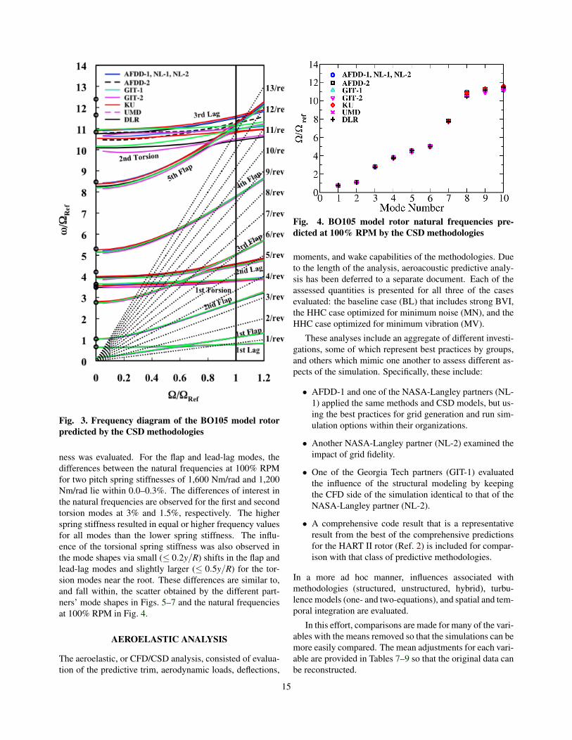
Fig. 3. Frequency diagram of the BO105 model rotorpredicted by the CSD methodologies

ness was evaluated. For the flap and lead-lag modes, thedifferences between the natural frequencies at 100% RPMfor two pitch spring stiffnesses of 1,600 Nm/rad and 1,200Nm/rad lie within 0.0–0.3%. The differences of interest inthe natural frequencies are observed for the first and secondtorsion modes at 3% and 1.5%, respectively. The higherspring stiffness resulted in equal or higher frequency valuesfor all modes than the lower spring stiffness. The influ-ence of the torsional spring stiffness was also observed inthe mode shapes via small (≤ 0.2y/R) shifts in the flap andlead-lag modes and slightly larger (≤ 0.5y/R) for the tor-sion modes near the root. These differences are similar to,and fall within, the scatter obtained by the different part-ners’ mode shapes in Figs. 5–7 and the natural frequenciesat 100% RPM in Fig. 4.

AEROELASTIC ANALYSIS

The aeroelastic, or CFD/CSD analysis, consisted of evalua-tion of the predictive trim, aerodynamic loads, deflections,

Fig. 4. BO105 model rotor natural frequencies pre-dicted at 100% RPM by the CSD methodologies

moments, and wake capabilities of the methodologies. Dueto the length of the analysis, aeroacoustic predictive analy-sis has been deferred to a separate document. Each of theassessed quantities is presented for all three of the casesevaluated: the baseline case (BL) that includes strong BVI,the HHC case optimized for minimum noise (MN), and theHHC case optimized for minimum vibration (MV).

These analyses include an aggregate of different investi-gations, some of which represent best practices by groups,and others which mimic one another to assess different as-pects of the simulation. Specifically, these include:

• AFDD-1 and one of the NASA-Langley partners (NL-1) applied the same methods and CSD models, but us-ing the best practices for grid generation and run sim-ulation options within their organizations.

• Another NASA-Langley partner (NL-2) examined theimpact of grid fidelity.

• One of the Georgia Tech partners (GIT-1) evaluatedthe influence of the structural modeling by keepingthe CFD side of the simulation identical to that of theNASA-Langley partner (NL-2).

• A comprehensive code result that is a representativeresult from the best of the comprehensive predictionsfor the HART II rotor (Ref. 2) is included for compar-ison with that class of predictive methodologies.

In a more ad hoc manner, influences associated withmethodologies (structured, unstructured, hybrid), turbu-lence models (one- and two-equations), and spatial and tem-poral integration are evaluated.

In this effort, comparisons are made for many of the vari-ables with the means removed so that the simulations can bemore easily compared. The mean adjustments for each vari-able are provided in Tables 7–9 so that the original data canbe reconstructed.

15

Fig. 5. Flapping mode shapes predicted by the CSDmethodologies

Fig. 6. Lead-lag mode shapes predicted by the CSDmethodologies

In addition to the comparisons evaluated using rotor az-imuth (time) as the independent variable, a statistical anal-ysis of the data was also included to help assess the accu-racy of the simulations. Bousman (Refs. 62, 63) introducedthe method of correlating the slope and scatter of computa-tions with experimental data to assess the overall accuracy.Figure 8 illustrates the concept of this analysis. The inde-pendent variable is the experiment data set, and a slope ofone indicates perfect correlation with experiment. Consis-tent over/under prediction will have a slope greater/less thanone. The slope should be used in conjunction with an as-sessment of the linear fit, which in this effort is the Pearsonproduct moment correlation coefficient, r. The correlationcoefficient is computed by dividing the covariance of two

16

Fig. 7. Torsion mode shapes predicted by the CSDmethodologies

variables by the product of their standard deviations:

r1 =∑( fc f d− fc f d)(gexp−gexp)√

∑( fc f d− fc f d)2 ∑(gexp−gexp)2(1)

where f and g are the independent and dependent variablemeans, respectively. For applications within this effort, thelinear correlations are all positive, indicating that overall thesimulations follow the direction of the data.

Rather than misusing the Pearson coefficient to indicatedata scatter, the sample standard deviation, s, is computedfor the residuals between experiment and computation, i.e.,

s =√

∑[( fexp− fc f d)− ( fexp− fc f d)]2 (2)

where the barred quantity is the mean of the residuals. Here,the closer to zero that this positive quantity approaches, theless data scatter about the linear regression line is observed.If one assumes a normal distribution about the regressionline (which may not be true), 68% of the data should liewithin one standard deviation (±1s) and 95% of the datawithin two standard deviations (±2s).

As with all statistical analyses, the size of the samplespace is important, so that the interpretation of the rotoraerodynamic loading where 360 computational samples areavailable is more accurate than the bending moments and tip

Fig. 8. Example statistical correlation of computationalvariables with experimental data

deflections where only 24 computational samples are avail-able.2 In addition, the presence of a few ‘outlier’ points isindicative of poor correlation of one or more features in thenonlinear data, which is not completely indicated in the lin-ear statistical analysis. Given the quantity of data analyzedin this work, only the summary statisticals are presented andnot the individual samples as seen in Fig. 8. These data arepresented as two column plots, one which plots the differ-ence between a perfect slope correlation (1) and the com-putational data (i.e., 1-computational slope), and a secondwhich plots the value of one standard deviation of the error(experiment - computation). The reader is cautioned thatthese statistical data should be used in tandem with the timehistory data to provide an accurate analysis of the predictionmethodologies.

ROTOR TRIM

To evaluate the predictive capabilities of the codes, the ro-tors should be trimmed to the same operational conditions.As discussed previously, the structural dynamics analysisensured that the rotor system was structurally modeled asclosely as possible across the partners’ CSD methods, sothat when the rotor is trimmed, the unknown variables as-sociated with the computational aeroelastic modeling arefurther reduced.

During the experiment, the freestream velocity and ro-tor shaft angle were prescribed. From these, a shaft an-gle correction for the wind tunnel interference effects wasextracted using the Heyson method (Ref. 64) and further

2The experimental data include 2,048 samples/rev forthe aerodynamic loads and 256 samples/rev for the struc-tural moments.

17

corrected using data from Brooks (unpublished; secondarycitation in Ref. 65). These corrections resulted in a flow de-flection of 0.8; so, an effective shaft angle of 4.5 relativeto the freestream velocity was applied in the computationalsimulations rather than the experimental 5.3 shaft angle.

The experimental uncertainties associated with the mea-sured forces and moments are 10 N and 10 Nm, respec-tively, based on the analysis of 32 revolutions of continuousmeasurements. These result in an uncertainty of 0.01 inthe collective angle and 0.04 in the cyclic control angles.

As described in each partner’s discussion regarding thesimulation details, the CFD/CSD solution was run until thetarget trim parameters (thrust and roll/pitch hub moments)were achieved within some predetermined criteria. By us-ing these criteria, the control angles and mean elastic twistwere extracted when trim was reached. These values areportrayed as deltas from the experimental trim values inFig. 9, with the corresponding experimental values givenin Table 6.

Table 6. Experimental trim control angles and meanelastic twist

Case Θ75 Θela ΘC ΘS

Baseline 3.8 -1.09 1.92 -1.34

Minimum Noise 3.9 -1.17 2.00 -1.35

Minimum Vibration 3.8 -1.18 2.00 -1.51

a Averaged over all four blades.

The control angles predicted by each partner are gen-erally similar and in the majority within 0.5 of the experi-mental values. The mean elastic tip twist is somewhat largerfor some cases, extending the difference up to ±1. In gen-eral, the CFD/CSD methodologies have the same tendencyof over- or under-predicting a particular control angle forthe same case. There is little difference between the trimangles when refining the grid (NL-2a and NL-2b), althoughlarger differences are noted when the same methods are runwith different grids/run options (AFDD-1 and NL-1) or dif-ferent CSD methods (GIT-1 and NL-2a).

Since the collective angle and the mean elastic tip twistcombine to provide the overall mean angle of the rotor, theycan be examined as a sum (Fig. 10). The error associatedwith scatter of the individual blade motion extends the ex-perimental data to 2.4–3.1, as indicated by the red arrowsoverlaid on the experimental data. Only two sets of theCFD/CSD simulations fall within this scatter band (NL-2,UMD) for all cases, while the others fall below the experi-mental scatter range for one or more cases. This is primarilydue to the larger negative mean tip twist predicted consis-tently by the CFD/CSD methods which tends to negate thecloser collective angle predictions. The experimental meanelastic tip twist is based on an average of the deflectionsfrom all four blades.

(a) Baseline

(b) Minimum noise

(c) Minimum vibration

Fig. 9. Rotor control angles and mean elastic tip twist attrimmed conditions relative to experimental values

18

Fig. 10. Sum of the collective angle and mean elastic tiptwist

There is no consistent trend to explain why someCFD/CSD methods fall within the scatter range and othersdo not. Turbulence modeling, temporal integration, compu-tational structural dynamics method, etc., all show no dis-tinct pattern from which to draw a conclusion. Van der Wallet al. (Ref. 2) suggest that the reason for this under predic-tion, which is also observed in many comprehensive meth-ods, is that the velocity normal to the rotor disk is underpredicted. This can be a result of either an under estima-tion of the wind tunnel blockage effects on the shaft angle,or that the influence of the wake on the rotor is under pre-dicted by the simulations. This latter scenario implies thatadditional wake refinement may be necessary. For at leastfor the NL-2 study, which examined a baseline and a refinedgrid, additional grid refinement does not influence the out-come significantly since the baseline grid results (NL-2a)were within the experimental bounds of four rotor blades.Further numerical optimization studies, including wake re-finement, may be warranted for the partner results that felloutside of the range.

AERODYNAMIC LOADING

The aerodynamic loading was evaluated by examination ofthe sectional airloads at the 87% radial station where exper-imental data were obtained. The normal force and pitchingmoment coefficients have been normalized for compress-ibility effects by multiplication of the squared freestreamMach number, M2. The experimental normal force andpitching moments were computed by integration of the 17Kulite R© pressures obtained along the 87% radial station.There has been a partial analysis to extract the differencesassociated with the integration of the BL aerodynamic load-ing with that of CFD simulation which includes hundreds oflocations along each radial station (Ref. 55). For the normalforces (CnM2), Boyd found that the effect of integration of

the full CFD resulted in a translational offset with the exper-imental data, but had little impact on the unsteady loading.His recommendation that these data be compared with ex-periment with the means removed has been adopted here.Differences for the pitching moment due to the integrationpatch, which was not examined in Ref. 55 may or may notbe significant. Varying results have been observed throughsimilar analyses of other configurations (Refs. 66, 67), inparticular for separated flow conditions.

The capability of the computational methods to predictthe aerodynamic loading has been assessed via two timehistory comparisons. The entire prediction (with meansremoved) are examined for one rotor revolution to assessoverall trends. BVI events in the first and fourth quad-rants of the rotor disk are also examined with the low-frequency content removed, allowing the high frequencycontent (11/rev and above) of the computations to be evalu-ated. While the experimental aerodynamic loading includes2,048 data points for each rotor revolution, the computa-tional data for each partner was gathered at 1 increments.To ensure that there is no bias introduced between the ex-periment and computations or between computations, alldata were filtered identically at 1 increments. This leadsto slight differences with the experimental data presented inRef. 2, but maintains consistency for this comparison.

As discussed previously, only the reference blade, blade1, was instrumented; and so, it resulted in a higher meanpitch and pitch oscillation magnitude compared to the re-maining experimental rotor blades. A blade-to-blade differ-ence was observed in the tip vortex strength for the experi-ment. This is not the case for the simulations, whose bladesare all comparable. Thus, in addition to the influence ofthe pressure tap integration, the experimental data can haveslightly higher means and magnitudes, although the latter ismitigated somewhat for the BVI events, which are causedby shed vorticity from all four blades.

Normal Forces The baseline case represents a descend-ing flight where strong BVI occurs, in this case at azimuthangles of approximately 50 and 300. For the minimumnoise and minimum vibration cases, the BVI is significantlyreduced or virtually eliminated at 50. The normal forces(means removed) predicted by the CFD/CSD analyses ap-pear to be overall comparable, as observed in Fig. 11, giventhe differences between grids, code algorithms, and struc-tural models. The largest scatter between CFD/CSD predic-tions exists for the baseline case, which was expected dueto the strong BVI.

For the baseline case, several features can be seen inFig. 11(a). While the S4 comprehensive code anticipatedby 5–10 the minimum loading (at 160) during the transi-tion from the advancing to the retreating side of the rotordisk, the CFD/CSD methods lagged experiment by 5. All

19

methods except DLR and UMD predicted the magnitude ofthe minimum loading within 0.01 of CnM2. Only the KUsimulation predicted the sustained normal force plateau be-tween an azimuth of 70 and 120. The GIT-1 predictionhad the smallest magnitudes for the main BVI events in thefirst quadrant, as well as a under prediction of the loadingfrom 0 to 40.

For the minimum noise case (Fig. 11(b)), the overallpredictions appear to be more consistent with one anotherand more accurate when compared to the experimental data.The full CFD/CSD and comprehensive methods except forGIT-2 predict the phase and magnitude of the normal forcevery well. Moderate overshoots in the peaks of 0.01-0.03CnM2 are observed for some of the methods. The hy-brid methods (GIT-2, UMD) show significant deviations inthe magnitudes at various locations (though not coinciden-tally); and they, along with the DLR comprehensive code,show more sensitivity to the BVI event in the first quadrant.The large over-prediction of BVI peak by these simplifiedmethods may be due to the lack of dissipation of the tipvortices that the full CFD methods encounter. In the hy-brid and comprehensive methods, the tip vortex strength ismaintained in the Lagrangian wake, with some empiricalmodeling to account for vortex aging. Dissipation in thehybrid methods will not occur until the vortex re-enters theRANS near-body blade grid. The vortex trajectory will alsoplay a role in the aerodynamic response, and as the two hy-brid models do not model the fuselage, this was examined.As will be shown later, however, the vortex tracks predictedby the computational methods, with and without fuselagemodels, are very similar.

All full CFD/CSD simulations for the minimum vibra-tion normal force case (Fig. 11(c)) show consistent trendsin both magnitude and phase. The peaks located about 90

and 180 are under predicted by 0.01–0.02, but the phaseis predicted within ± 2. The hybrid simulations indicatethat the magnitude of unsteady loading over a rotor revolu-tion is under predicted. This is particularly evident at the140 minimum loading location, where they under predictthe amplitude by 0.04-0.05. This under prediction couldbe an influence of the fuselage, as the DLR comprehensivemethod with the fuselage is able to predict the extent ofthe loading. Lim et al. (Ref. 52) did not observe a sim-ilar change in the aerodynamic loading when using a fullCFD/CSD (OVERFLOW/CAMRAD II) method with andwithout the fuselage.

Due to the number of CFD/CSD participants (10), thedata plots are expanded to examine the BVI events (or themitigation of these events) in the first BL quadrant.

Lim et al. (Ref. 52) noted that for their full CFD/CSDmethod, the influence of the fuselage was to increase themagnitude of the BVI events in the first quadrant, but therewere only minor changes in the BVI predictions in the

fourth quadrant. Interestingly, all of the unstructured meth-ods, to some degree, appear to be less influenced by thefuselage in the first quadrant, most dramatically for the BLcase (Fig. 12). AFDD-2 is the least affected, while GIT-1, which uses the same grid and CFD code, but a differentCSD method than NL-2a, is the most affected. The gridrefinement in NL-2b from 14 to 23 million grid nodes im-proves the predictions after 50, but has little effect in theoscillatory loading prior to 50. Computations were un-dertaken for the GIT-1 case varying the pitch spring stiff-ness (increase by 400 Nm/rad) and modifying the numberof subiterations with little discernable change in the pre-dictions for this region. All of the structured methods ap-plied higher-order spatial algorithms compared to the un-structured methods, which are limited to second-order ac-curacy.

For the MN and MV cases, the differences manifestthemselves in a smoother loading increase between 50–90 when compared to experiment and their structured fullCFD/CSD counterparts. These differences between struc-tured and unstructured methodologies were not observedfor the fourth quadrant, which agrees with the minor influ-ence of the fuselage observed by Lim et al. (Ref. 52). Theseobservations and additional computations suggest that thegrid may need to be refined in this area between the fuse-lage and rotor to capture these effects with the second-orderspatial schemes. The numerical aspect of the simulation isrecommended for further evaluation.

The low-frequency content of the normal forces has beenremoved, allowing the high frequency content (11/rev andhigher) of the computations to be assessed. Expanding thehigh-frequency content of normal forces in the first quad-rant (Fig. 13) highlights the differences between the sim-ulations and with experiment. Experimental data indicatetwo BL BVI events at 45 and 56, one MN BVI eventat 70 and three weaker MV BVI events at 40, 48, and58. Overall, the full structured CFD/CSD methods cap-ture the 80% or more of the amplitude of the BVI events,but encounter phase shifts of up to 6. The unstructuredmeshes have mixed success with capturing the amplitudesfrom AFDD-2 (60–80%) to the NL-2a/GIT-1 coarse meshpredictions (50% or less). The phase shift observed withthe unstructured methods are comparable to or better thantheir structure method counterparts. The GIT-2 hybrid re-sults generally over predict the BVI amplitudes, except forthe strong MN BVI event which is under predicted. Theother hybrid method, UMD, indicates mixed success for theamplitude predictions. For the BL and MV cases, the hy-brid and comprehensive methods are marked by additionallarge events beyond 60, which is indicative of higher elas-tic twist response, as discussed later. The single strong MNBVI event is predicted by the structured methods, albeit atreduced amplitude and up to a 10 phase shift. It is notpredicted by the unstructured methods, indicating the im-

20

portance of the grid, as discussed previously. The phase ofthe multiple MV weaker BVI events prove to be the mostdifficult to predict in phase, and no conclusions between thevarious predictions can be drawn.

In the fourth quadrant, the dependence on full CFD/CSDvariables appears less pronounced and comparisons withexperiment are more favorable, as observed in Fig. 14.Overall the magnitude and phase of the BVI events are well-predicted, within 0.01 and ±2–4 by the full CFD/CSDpartners. The DLR (S4) comprehensive method overall pre-dicts the phase of BVI events well, with an over predictionof the peak (within 0.03) of multiple BVI events but withgood phase predictions. The hybrid methods miss some ofthe BVI phase predictions by up to 10 (GIT-2, lag; UMD,lead). Their magnitudes, once corrected for these phase dif-ferences, correlate relatively well with the full CFD/CSDpredictions. These phase differences may be due possiblyto the missing influence of the fuselage, which is includedin the comprehensive solution (DLR). The DLR prediction,in addition to the full CFD/CSD methods, does not mani-fest the larger phase shifts observed by the hybrid methodswithout the fuselage.

The visual inspection of the prediction time histories canbe augmented with statistical analysis to aid in evaluationof the predictions compared with experimental data. Thisquantitative analysis examines the deviation of the compu-tational predictions with the experimental data. This is eval-uated by plotting the experimental data as the independentvariable and the computational data as the dependent vari-able. A slope of 1.0, combined with a Pearson coefficient(r) of 1.0 indicates perfect linear correlation with experi-ment.

The statistical analysis of the normal force coefficientresiduals in Fig. 15 shows some interesting trends. The cor-relations are above r = 0.84 for all methods and cases (notshown), implying a strong linear correlation. The slopes areprimarily within 5%-10% for the baseline case, with the ex-ceptions of GIT-1, UMD, and DLR (comprehensive code).The standard deviation indicates the presence of some largeexcursions. For example, while GIT-2 has one of the mostaccurate slopes, it also has the largest standard deviation,indicating that the data have phase differences, so that anerror band of 0.02 must be used to ensure that 68% of thepredictions fall within this band. Conversely, GIT-1 has alarger slope deviation, but 68% of the predicted values liewithin 0.01 (and 95% lie within 0.02) of the experimentalCnM2 values. Examining these in conjunction with the timehistories in Figs. 11, 13 and 13, the large scatter of GIT-2 is due to phase shifts in the BVI predictions, which aresometimes significant, while the higher slope deviation ofGIT-1 is due to the (lack of) BVI predictions in the firstquadrant. An analysis was undertaken to extract the phaseshift from the data, for example, GIT-2, and re-examine thestatistics. These yielded mixed results as methods exhibit

(a) Baseline

(b) Minimum noise

(c) Minimum vibration

Fig. 11. Normal force predictions at 87% radial station,means removed and normalized by M2

21

Fig. 12. Comparison of the BL normal force predictionsin the first rotor disk quadrant at 87% radial station,means removed and normalized by M2

both positive (lead) and negative (lag) offsets in the phaseprediction of both BVI and mean (low frequency) events.Thus, the statistical analysis includes all data, regardless ofobserved phase offsets, and the reader is again encouragedto use these statistical data in conjunction with the time his-tories.

Overall the KU simulation appears to be most statisti-cally accurate of the methods with a relatively small errorin the slope and the smallest scatter. Upon examination ofFigs. 11, 13 and 13, it is apparent that this simulation cap-tures many of the features with both small amplitude andphase error.

Similar observations can be drawn for the minimumnoise and vibration cases, where, taken together with thescatter, the comparable methods are overall similar in theirpredictive accuracy of the normal force. The hybrid andcomprehensive methods appear, in general, to have 50%-100% larger magnitude slope and standard deviations com-pared to the average of the full CFD/CSD results. Since thecomprehensive method appears to be more statistically ac-curate than the hybrid methods, one may hypothesize thatthe lack of the fuselage may be a contributory factor.

Pitching Moments A similar analysis to the normal forcewas undertaken for the aerodynamic pitching moment forall three cases. The full revolution (Fig. 16), first quad-rant high frequency (Fig. 17), and fourth quadrant high fre-quency (Fig. 18) pitching moments have been plotted usingthe same line definitions applied for the normal forces.

In general, for the full revolution (Fig. 16), the pitch-ing moment appears to be similarly predicted by all meth-ods, though the KU results do not capture the extent of thepitching moment recovery at about 110, with a subsequent

(a) Baseline

(b) Minimum noise

(c) Minimum vibration

Fig. 13. First quadrant normal force predictions at 87%radial station, means removed and normalized by M2

22

(a) Baseline

(b) Minimum noise

(c) Minimum vibration

Fig. 14. Fourth quadrant normal force predictions at87% radial station, means removed and normalized byM2

(a) Normal force slope correlation

(b) Normal force error standard deviation

Fig. 15. Sectional normal force residual statistical cor-relation at 87% radial station. Normal force coefficienthas the means removed and normalized by M2

translation offset until the recovery at 190 azimuth. Mostof the methods, with exception of the GIT-1 results overpredict the pitching moment about 260 by about 0.0005–0.001 CmM2.

Unlike the normal force, the methods do not align as ac-curately with one another for the minimum noise pitchingmoment. Most full CFD/CSD methods predict the behav-ior from 100 to 260 consistently, with overshoots at thepitching moment peaks at about 135 and 260, but overpredict the magnitude of the minimum moment at about190 by 0.0002-0.0005. The phase of the minimum mo-ment is well predicted with the exception of the KU thatleads, and DLR and GIT-1 that lag the minimum by about10. KU’s prediction has similar characteristics as its BLprediction, while the UMD, DLR and GIT-2 results equalor slightly under predict the magnitudes of the peaks, withvarying phase lags.

The minimum vibration pitching moment is more con-

23

sistent, with similar differences observed for the KU,AFDD-2 and DLR results. The remainder of the methodsfall within 0.0005 of the peak magnitude and ± 5 of theazimuthal location.

The expansion of the first quadrant pitching mo-ments, including the removal of the low-frequency con-tent (Fig. 17) illustrates that the overall levels in the base-line case are predicted within 5–10% by the full CFD/CSDmethods, with a phase shift of approximately 5–6 of theBVI events. The characteristics of the methods in predictingthe normal force remain relatively consistent here: underpredictions by the unstructured methods and over predic-tions by the hybrid (GIT-2, UMD) methods for the same az-imuthal regions. The comprehensive code tends to predictthe pitching moments similar to many of the full CFD/CSDmethods. This indicates the importance of the fuselagemodeling when comparing to the hybrid results without thefuselage. The structured full CFD/CSD methods over pre-dict slightly the magnitude of the oscillations. For mostmethods, the BVI reaction persists beyond 60 azimuth un-til 90–120, depending on the method. The improved nor-mal force correlation of KU with experiment compared tothe rest of the computational methods for the baseline caseis not readily apparent here.

The strong BVI event between 65 and 90 azimuth inthe minimum noise case is predicted most accurately by theAFDD-1 simulation, which captures the sharp peaks andvalleys, with little phase lag. The remainder of the fullCFD/CSD methods capture only a portion of the BVI event,with residual oscillations between 75 to 120. The GIT-2and UMD hybrid methods over predict the oscillatory mo-tion, while the DLR comprehensive method again is consis-tent with most full CFD/CSD methods.

For the first quadrant of the minimum vibration casewhere three weaker BVI events are located, the AFDD-1accuracy observed for the MN case is not repeated; it andKU over predict the BVI amplitudes by a factor of abouttwo, and includes a phase offset of about 5. The remainderof the structured full CFD/CSD methods capture the mag-nitudes well, but the BVI peaks are 0 to 180 out of phasewith experiment, depending on the method. Once again, theunstructured methods predict weaker BVI response, whilethe hybrid and comprehensive methods over predict the am-plitude by a factor of 2–3, with phase offsets of 0–10,which vary with method and BVI event.

In the fourth quadrant, the NL-1 predictions are over-all the most accurate for the baseline case, though that isnot true for the minimum noise and vibration cases. For allmethods, there are features that are well predicted but othersthat are not, even within the same case. Overall, the levelsand general features of the pitching moments exclusive ofthe BVI events are captured by all methods, although some(e.g., KU, UMD and GIT-2) exhibit large spurious oscilla-

tions.

The statistical analysis of the pitching moment coeffi-cient in Fig. 19 indicates some differences from the normalforce analysis. The correlations are not as strong as the nor-mal forces, remaining above 0.6 for all methods and cases,but still provide a relatively strong linear correlation. Un-like the normal force, where overall similar predictive be-havior of each code was observed, there is widely varyingcapability of most methods across the three cases, as de-noted by the differences in the slopes. The scatter is moreconsistent across each test case and most methods, with be-tween 0.005–0.001 CmM2. Comparing each test case, thehybrid methods (GIT-2, UMD) show less accurate correla-tion than their full CFD/CSD counterparts, and the com-prehensive code (DLR) is overall comparable with the fullCFD/CSD methods. The 64% increase in the grid density,likewise has no discernible influence on the statistical prop-erties of the pitching moment. Application of the sameCFD/CSD methodology, but using different grids and runproperties indicates only differences in statistics (AFDD-1, NL-1). The influence of time step and/or turbulence isclearly apparent, in that the KU prediction, run at a stringenttemporal integration, combined with a higher-order spatialscheme and two-equation turbulence model, shows a signif-icant improvement in the slope correlation. This improve-ment has also been observed for hybrid RANS-LES turbu-lence methods run on refined grids and time steps for theUH-60A undergoing dynamic stall (Refs. 68, 69). The KUover prediction of the BVI events is clearly reflected in thescatter (standard deviation), which is comparable with thehybrid methods.

BLADE TIP MOTIONS

The aerodynamic loading results in the elastic deflection ofthe rotor blades, which is examined next. The blade tip mo-tion is defined in this effort as the elastic deflection with-out inclusion of, and relative to, rigid rotor motion and set-tings such as the pre-cone and pre-twist of the blade andthe blade pitch control angles (including HHC for MN andMV cases). The tip deflection azimuthal time history hasbeen selected to provide an assessment of the tip motions.During the experiment, the motion of all four blades weremeasured. Due to different instrumentation on each blade,the blades exhibit some differing motion, and the motionfor all four blades is presented. Blade 1, the nominal refer-ence blade, was found to always have a an increased flap-ping and elastic twist compared to the other blades due tothe presence of numerous pressure sensors which modifiedthe elastic properties of the blade. The motion of blade 4 issimilar to that of blade 1, as it also was fitted with pressuresensors, while blades 2 and 3 were not modified. These dif-ferences are reflected during the integrated properties of therotor, such as thrust.

24

(a) Baseline

(b) Minimum noise

(c) Minimum vibration

Fig. 16. Pitching moment predictions at 87% radial sta-tion, means removed and normalized by M2

(a) Baseline

(b) Minimum noise

(c) Minimum vibration

Fig. 17. First quadrant pitching moment predictions at87% radial station, means removed and normalized byM2

25

(a) Baseline

(b) Minimum noise

(c) Minimum vibration

Fig. 18. Fourth quadrant pitching moment predictionsat 87% radial station, means removed and normalizedby M2

(a) Pitching moment slope correlation

(b) Pitching moment error standard deviation

Fig. 19. Sectional pitching moment residual statisticalcorrelation at 87% radial station. Pitching moment co-efficient has the means removed and normalized by M2

The experimental data were recorded in increments of15, which was repeated for 100 revolutions and averaged.The measured tip blade motion including 6/rev componentswas synthesized from a Fourier analysis of the averaged sig-nal using three flap modes, two lag modes and two torsionmodes. These data have been shown to have an error withinthe accuracy of the original measured motion (Ref. 70).

Statistical analyses were again performed for the compu-tational predictions. The data were reduced to 15 intervalsor 24 samples per case, as this resolution is sufficient sinceonly lower harmonics are present in the blade motion. Thereduction in the number of samples results in a lower levelof confidence than that for the aerodynamic loads analysis,but they are useful for revealing trends.

Flap Deflection The trimmed elastic flapping responsefor all cases examined is shown in Fig. 20. For all threecases examined, the flapping motion peaks between 270

26

and 280 azimuth and reaches a minimum between 80 and100. The minimum noise case also indicates the presenceof a secondary elastic maximum at approximately 40–50.Both the minimum noise and vibration cases have a saddlepoint about the 180 azimuth location.

The full CFD/CSD simulations overall tend to predictthe characteristics and phase of the flapping deflections.The scatter including all methods is on the order of 1–2 cm(0.5–1 ordinate units) or about 0.5 cm for most methods (ex-cluding UMD, GIT-2 and AFDD-2), and results primarilyfrom the differences in the amplitude predictions. The av-erage scatter from the experiment varies between 0.55–0.65cm, with maximums of up to 1.4 cm. The saddle points arepredicted by all methods for the minimum vibration caseand by all but AFDD-1 for the minimum noise case.

Statistically comparing to the motion of blade 1(Fig. 21), the overall accuracies can be assessed over afull rotor revolution. The results across most predictions(AFDD-1, KU, NL-1, NL-2, UMD and DLR) are consis-tent, no matter which case is considered. Two of the un-structured methods (GIT-1 and AFDD-2) have some devi-ation with the experiment, which is due primarily to thephase shift observed in the time history data (Fig. 20).

There is no indication that grid refinement improvesthe simulations (NL-2 cases are equal), The trend betweenthe two partners running the same methodologies indepen-dently (NL-1 and AFDD-1) is inconclusive with respect tothe slope accuracy but is consistent in the scatter. The meth-ods are less accurate in predicting the minimum vibrationand baseline cases compared to the minimum noise case.The CFD/CSD methods do not have appear to have anyadvantage in predicting the flap motion compared to theless expensive comprehensive method (DLR). The lack ofa fuselage model is not apparent in the accuracy of thesepredictions either.

Lead-Lag Deflection The lead-lag deflection is next eval-uated, where xel is defined as positive for deflectionscounter to the rotation direction, i.e., lag deflections. Com-parisons of the computational simulations with experimentshow a consistent translational offset of about 2–4 cm(0.57–1.14 lag angle), which was not able to be resolvedduring the HART II data analysis and is consistent withanalyses of other computational methods of varying fidelity(Ref. 2). Thus, the means were removed for the analysishere. The mean values are listed in Tables 7, 8, and 9.

The in-plane tip deflections for all three cases result in a1/rev motion that has its most forward location at 180 andreaches its most aft position at 0, and these motions areimpervious to the application of the 3/rev HHC in the min-imum noise and vibration cases. Only minor differencesbetween the CFD simulations and the experiment are ob-served for the tip lead-lag deflections in Fig. 22, with the

(a) Baseline

(b) Minimum noise

(c) Minimum vibration

Fig. 20. Blade tip flap deflections relative to pre-cone

27

(a) Deviation of the slope correlation

(b) Exp.–Comp. error standard deviation

Fig. 21. Blade tip flap deflection residual statistical cor-relation relative to pre-cone

exception of the AFDD-2 simulations, which shows a phaselead of about 10. The GIT-2 simulation also shows a simi-lar phase shift forward of 180 maximum for the MN case.The differences between CFD/CSD coupling and the com-prehensive analysis (DLR) is seen primarily in a reductionof the magnitude of the deflection predicted by the compre-hensive code.

These phase offsets and magnitude reductions are re-flected in the statistical analysis of the deflection residuals,shown in Fig. 23. The remainder of the CFD/CSD simula-tions have excellent correlation with experiment (typicallywithin ±5%) for all cases, and the scatter is minimal, withdifferences of 0.1 or less.

Elastic Twist The delay of the BVI events in the first quad-rant observed in the aerodynamic loads (Figs. 13 and 17)can be in part correlated with the predicted behavior of theelastic twist (Fig. 24), where CFD/CSD predictions showa phase lag of the peak observed at 90 during the experi-

(a) Baseline

(b) Minimum noise

(c) Minimum vibration

Fig. 22. Tip lead-lag deflection with means removed(Lag deflections are positive.)

28

(a) Deviation of the slope correlation

(b) Exp.–Comp. error standard deviation

Fig. 23. Tip lead-lag deflection statistical correlationwith means removed

ment. While some partners’ results predict the blade 1 twistlevels at 0 quite well (NL-2, KU, UMD, AFDD-2), oth-ers (AFDD-1, NL-1, GIT-1, GIT-2) under predict the twistby approximately 1. All partners except the two hybridmethods (GIT-2 and UMD) predict the 2/rev content of thebaseline twist.

The 3/rev behavior of the elastic twist is generally pre-dicted consistently by the different computational methodsfor the MV and MN cases. The GIT-2 simulation continuesto have a translational offset and lower amplitude oscilla-tions. The other hybrid method, UMD, is tends to predictthe magnitudes and mean of the elastic torsion more accu-rately than the GIT-2 hybrid method. The AFDD-1 simula-tion shows a translational offset of 1.2 and -1 for the MNand MV cases, respectively, but captures the phases. Theseoffsets do not appear to translate into a conclusive differen-tial in the aerodynamic loading (Figs. 14 and 18) or, as willbe seen, the torsional moments (Fig. 30).

The statistics associated with the residuals of the elas-

(a) Baseline

(b) Minimum noise

(c) Minimum vibration

Fig. 24. Blade tip elastic twist relative to the pre-twistand blade controls

29

tic twist at the blade tip (Fig. 25) reflect the behavior ob-served in the time history plots. The large excursions notedfor AFDD-2 and DLR in the baseline case, and AFDD-1in the MN case are clearly reflected. Scatter varies fromabout 0.4 (one standard deviation) for the baseline case toalmost double that value for some methods for the MV andMN cases. The correlation tends to be less positive for theelastic twist than for other variables, but this is not unex-pected as the comparison is with blade 1, which is known tohave a higher mean and larger elastic deformations, whichis reflected in the comparisons.

Once again, there appears to be little return for the in-creased grid refinement of the NL-2 computations. The dif-ference in the OVERFLOW-CAMRADII runs by AFDD-1and NL-1 indicate that the higher fidelity DES model andrefined grid does not appear to have much benefit. Whilethe CFD/CSD simulations provide a better prediction of theelastic twist for the baseline case, the same conclusion isnot true for the MN case and in most instances for the MVcase.

Structural Moments

Strain gauges were placed on rotor blade 1 to measure theflap and lead-lag bending moments at 17%R and the torsionmoment at 33%R. Only the dynamic (means removed) arecompared as the strain gauge calibration was performed forthe non-rotating system, and it is suspected that bias due tothe centrifugal forces may cause a translational or mean off-set. The data for the experimental were obtained by averag-ing the measured moments from 32 continuous revolutions.

The partners used two different approaches in comput-ing the structural moments: the modal method and the forcesummation method. The modal method computes the bend-ing moments (both transverse and in-plane) using the rela-tion of the moment to the curvature (second derivative of themodal deflection multiplied by the bending stiffness) andthe torsional moment using the relation of the moment tothe twist change (first derivative of the modal twist multi-plied by the torsional stiffness). Numerical errors associ-ated with the computation of these derivatives may exac-erbate the errors associated with the use of a few modes.The force summation integrates the forces radially outwardfrom the reference location with its associated moment arm.While more computationally intensive, this approach tendsto be more exact, in particular when a linear (modal) anal-ysis is applied instead of the exact nonlinear representationof the structural dynamics of the rotor.

Flap Bending Moments The flap bending moments areexamined at the radial station located at 0.17R (from thehub center) where the largest curvature of the flap modes isobserved (see for example, the fourth and fifth flap modes

(a) Deviation of the slope correlation

(b) Exp.–Comp. error standard deviation

Fig. 25. Blade tip elastic twist residual statistical corre-lation with means removed

in Fig. 5). van der Wall et al (Ref. 2) notes that for theseHART II cases that comprehensive codes show a lack ofcorrelation with the experiment, leading to unsatisfactorypredictions of this parameter.

Figure 26 presents the CFD/CSD predictions of the flapbending moments for the 17% radial station. The 2/rev be-havior of the flap bending moment is captured by most ofthe methods. albeit with large differences in both the am-plitude and phase in some predictions.

This does not carry over to the minimum noise andminimum vibration cases, where the two DYMORE-based(force summation) simulations appear to capture the behav-ior of flap bending moment more accurately in phase thanthe other models applying modal approximations. The ob-servation cannot be applied to the RCAS (AFDD-2) simu-lations, however, which also applies the force summationmethod. The overall amplitude is under predicted. Themodal-based simulations tend to over predict the bendingmoments with a 20–30 lead in phase.

30

Statistically in Fig. 27, it is clear that the CFD/CSD pre-dictions for the flap bending moment have significant er-rors. On average, the slope correlation is in error by morethan 30–40%, with some methods including scatter that is30–40% of the amplitude of the moment. The less accu-rate prediction of the flap bending moment compared to theother parameters of interest merits further investigation.

Lag Bending Moments The trend of the lag bending mo-ments at 17% radial station is accurately predicted by thecomputational methods, as seen in Fig. 28 and clearly mim-ics the 1/rev motion in the lead-lad deflection (Fig. 22).This is true of the baseline, minimum vibration and noisecases. The maximum of the bending moments located be-tween 90 and 270 is over predicted by the some of thecomputations up to 50%. The flattened plateau behavior isnot predicted by the GIT-2 and UMD hybrid methods, but ispredicted by the full CFD/CSD methods. For the minimumnoise and minimum vibration cases, the AFDD-2 simula-tion is the most accurate, but it significantly over predictsthe moment for the baseline case. The NL-1 and KU sim-ulations consistently predict the trends most accurately forall the cases, followed closely by the NL-2 and AFDD-1simulations. The grid refinement study of NL-2 shows noinfluence on this structural variable.

Figure 29 illustrates the scenario where the overall shapeof a function is well predicted; but the amplitudes are, forthe most part, over predicted. The over prediction of theamplitude of the lag bending moment is seen through thenegative difference between the perfect fit (1) and the slopeof the computational data. The standard deviation indicatesthe impact of this overshoot in amplitude. The largest over-shoot (exempting the phase lag from AFDD-2) is seen tobe GIT-2, which has an overshoot of 20–25 Nm, which isthe amount shown in Fig. 29. Overall the best correlationsappear to be the NL-1 and KU simulations, which combinehigher fidelity turbulence modeling with small time steps.

Torsion Moments The torsion moment is assessed at the33% radial station where the second torsion mode reachesa minimum (Fig. 7). The torsion moments are shown inFig. 30. As with the lag bending moment, the torsion mo-ment is consistently predicted by the CFD/CSD methodolo-gies. The overall amplitude of the torsion is predicted wellfor the baseline and minimum noise cases, and slightly un-der predicted in the minimum vibration case for most meth-ods. There is a phase shift introduced by the GIT-2 hybridmethod. There is minimal influence from the grid refine-ment, as observed by the superposition of the two NL-2aand NL-2b curves. The AFDD-2 simulation also showssome sensitivity to the minimum noise case, though thepresence of a 10 phase lead, and a corresponding 40% de-crease in the amplitude. This is not the circumstance in the

(a) Baseline

(b) Minimum noise

(c) Minimum vibration

Fig. 26. Flap bending moment predictions at 17% radialstation with means removed

31

(a) Delta of the slope correlation

(b) Exp.–Comp. error standard deviation

Fig. 27. Flap bending moment statistical correlation at17% radial station with means removed

minimum vibration case.

Statistically, the torsion moment has moderate correla-tion with experimental data as the slopes fall within 10–20% of the perfect correlation line. One standard deviationfalls within 1 Nm for the baseline case and 2 Nm for theminimum noise and vibration cases. The grid refinementhas a significant impact on the scatter when the NL-2a gridis refined to NL-2b for the HHC cases, though it does nothave a significant influence for the baseline case. The com-prehensive method has less success overall in correlatingwith experiment than its CFD/CSD counterparts, althoughthe scatter remains approximately the same or better at 1Nm for all cases.

VORTEX LOCATIONS

The vortex trajectories were measured experimentally attwo blade azimuth location of 20 and 70 for a varietyof radial stations. Here, data at the 70% lateral position

(a) Baseline

(b) Minimum noise

(c) Minimum vibration

Fig. 28. Lag bending moment predictions at 17% radialstation with means removed

32

(a) Delta of the slope correlation

(b) Exp.–Comp. error standard deviation

Fig. 29. Lag bending moment statistical correlation at17% radial station with means removed

(y = ±1.4m), where BVI are encountered, are extractedfrom the CFD/CSD results, as well as from the comprehen-sive code (DLR), and compared with experiment. The ex-perimental locations were computed from 100 vortex centerpositions isolated from PIV measurements.

For the CFD/CSD simulations, the vortex locations wereidentified by the center of the location where the largest vor-ticity was observed. This was typically by visual inspectionand interpolation of contour plots, such as the sample in-cluded as Fig. 32. Thus, there may be an additional errorfrom this exercise with regard to the location of the vortices.

The NL-2 partner provided vortex locations for only NL-2a, as the two simulations appeared to have the same pre-dicted vortex tracks.

Advancing side The advancing side vortex positions aregraphically illustrated in Fig. 33, where the experimentalopen symbol is the vertical position of the reference blade1 at the reference position of about 135 azimuth. Since

(a) Baseline

(b) Minimum noise

(c) Minimum vibration

Fig. 30. Torsion moment predictions at 33% radial sta-tion with means removed

33

(a) Delta of the slope correlation

(b) Exp.–Comp. error standard deviation

Fig. 31. Torsion moment statistical correlation at 17%radial station with means removed

the vortex positions were measured by using blade 1, whichhas higher mean flapping position than the other blades, thevortex position extracted from the computational results isexpected to appear below that position.

This artifact is observed for all the computational resultswith the exception of the UMD predictions for all of thecases, and AFDD-1 for the MN case. The curved track ofthe vortex is predicted well by all methods except the GIT-1simulations. The scatter is somewhat expected given the ad

Fig. 32. Example vorticity plot to locate the tip vortexpositions

(a) Baseline

(b) Minimum noise

(c) Minimum vibration

Fig. 33. Tip vortex trajectories, advancing side y = 0.7R(The blade tip location is denoted by the open symbol.)

34

hoc method of extracting these values, but overall, the dif-ferent computational methods predict the values within 5%of the rotor radius (0.1 m). The KU vortices and AFDD-1vortex tracks are consistently the most accurate of the part-ners’ across all three cases, and this is reflected in the priorobservations that these methods provide some of the mostconsistent results. The NL-1 positions, exclusive of the aftportion of the minimum noise case is also very accurate.The lower position of the vortex track for NL-2 and GIT-1 is not unexpected given the smaller influence of the BVIin the aerodynamic loading (Figs. 13 and 17) through thelower amplitudes of the oscillatory loading.

There is a counter-rotating vortex that appears on theadvancing side of the MV case, which is indicated inFig. 33(c) as the second set of filled squares. The counter-rotating vortices were observed in the CFD/CSD simula-tions, but as only one partner provided that data, the com-parisons are not included here.

Retreating side The predicted vortex tracks from the sim-ulations are much more accurate on the retreating side(Fig. 34), which is also not unexpected due to the moreconsistent results observed for the aerodynamic loading(Figs. 14 and 18). Most of the partners results are sur-prisingly coincident given the method of obtaining the loca-tions. The prescribed wake comprehensive code computa-tions by DLR, show relatively comparable position trackingfor both the advancing and retreating sides, indicating thatthe additional computational effort for CFD/CSD couplingis not necessary for this parameter.

CONCLUSIONS

There are many factors affecting the accuracy of aCFD/CSD coupled analysis. In most cases, the CFD codehas the greatest impact on the quality of the simulations.

• In the HART II case where the interaction betweenthe blades and their trailed vortices is of major con-cern, a certain level of higher-order numerical schemesin either the spatial discretization process or the timeadvancing algorithm is believed to be crucial for en-hanced predictions. In addition, the off-body gridspacing, grid refinement techniques, time step sizecoupled with the number of subiterations, and soon are the important contributors. For a RANS(Reynolds-Averaged Navier-Stokes) calculation, theturbulence model should be properly incorporated inthe analysis, but the influence of different turbulencemodels studied thus far does not appear to have a sig-nificant impact on the solution accuracy.

• The full CFD/CSD methods predicted relatively com-parable behavior for the normal force and pitching mo-ments using similar turbulence models and temporal

(a) Baseline

(b) Minimum noise

(c) Minimum vibration

Fig. 34. Tip vortex trajectories, retreating side y =−0.7R (The blade tip location is denoted by the opensymbol. )

35

integration. Larger temporal integration, in particu-lar with second-order spatial schemes appear to misssome of the BVI events on the advancing side of therotor disk. The most accurate correlations paired atwo-equation turbulence model with small time steps.Improvements using the same methodology with a de-tached eddy simulation and smaller time steps werealso observed. These are comparable to observationsfrom the UH60A workshop for rotor simulations withdynamic stall (Refs. 68, 69).

• The BVI events associated with the advancing rotordisk are influenced by the fuselage, while the events onthe retreating side of the rotor disk are not sensitive tothe fuselage. The results from unstructured methods,which currently apply second-order spatial schemes,indicate the need to improve the quality of the grid inthis area to capture these events. The advances un-derway for higher-order discontinuous Galerkin meth-ods for unstructured methods should alleviate some ofthis, as noted by the improved predictions by the struc-tured methods that apply fourth- to sixth-order spatialschemes. In particular, the baseline HART II case willprovide an excellent case to test these new schemes.

• Additional grid refinement (from a nominal engineer-ing quality grid) appears to be less influential thanother CFD parameters, such at time step and turbu-lence modeling.

• Two hybrid methods examined have mixed results inaccuracy. These methods over predict some of thecharacteristics of the BVI in the first quadrant. Asthis behavior is not observed for the most part by thecomprehensive code nor the full CFD/CSD methods,which all include a fuselage model, the less accuratepredictions point to the lack of modeling the fuselage.The development of a fuselage model, perhaps similarto that within the S4 comprehensive code, appears tobe warranted.

• Computation correlation with experiment for the nor-mal forces is more accurate than pitching moments, asexpected. Lead-lag deflections and lag bending mo-ments are accurately predicted by the almost all ofthe methods, regardless of the different computationalmethods and options.

• Blade elastic twist predictions, as characterized bythe tip deflections, are predicted well by many of thefull CFD/CSD methods. This prediction, in concertwith accurate predictions of the unsteady flap oscil-lations, appears to be important for accurate aerody-namic loading at the outboard location where BVI oc-curs. There appears to be less correlation of the predic-tion of the vortex locations with the accuracy of theseother variables related to BVI.

• The observations associated with the vortex locationcompared with the rotor elastic deflections and aero-dynamic loading suggest that the vortex strength is an-other parameter of interest that should be studied withCFD/CSD simulations. It is already a parameter eval-uated with comprehensive codes, but it has not beenexamined in detail with CFD/CSD methods. In par-ticular, the dual-vortex pair that is observed with theminimum vibration case has not be examined by mostof the partners due to the labor intensive requirementsto extract the vortex characteristics from the CFD/CSDflow field.

• Most current CFD/CSD analyses apply an off-bodygrid spacing of 10% chord length, which is signifi-cantly larger than the actual vortex core size as notedduring the HART II wind tunnel test. The influence ofgrid adaptation strategies under development on wakecore size is recommended for quantitative evaluationwith respect to the accuracy of the variables of inter-est.

• While the CFD/CSD methods more accurately predictthe flap bending moments compared to comprehensivecodes (Ref. 2), analysis of predictive capabilities forboth the CFD and CSD modules needs further inves-tigation, as no clear consensus exists with the set ofCFD/CSD methods evaluated.

ACKNOWLEDGMENTS

The authors would like to acknowledge the support ofHART II partners: DLR, DNW, NASA, Onera, and AFDD.In addition, the authors would like to thank all of their col-leagues, students, or advisors for their collaboration:

AFDD-2: Andy Wissink, Anubhav Datta, Mark Pots-dam, Venke Sankaran, Jay Sitaraman, and Roger Strawn ofthe Helios development team.

GIT-1: Michael Acierno and Nicolas Reveles, GraduateResearch Assistants at the Georgia Institute of Technology,and Dr. C. Eric Lynch, a graduate of the Georgia Instituteof Technology. Prof. Olivier Bauchau of the Shanghai JiaoTong University provided insights to permit the modifica-tion of DYMORE4 for HHC.

GIT-2: Prof. Lakshmi N. Sankar and Dr. Kyle Collinsof the Georgia Institute of Technology. Prof. OlivierBauchau provided DYMORE2.

KU: Young-Hyun You and Jeong-Hwan Sa, GraduateResearch Assistants at Konkuk University.

NASA-LaRC: Elizabeth M. Lee-Rausch of the NASALangley Computational AeroSciences Branch for generat-ing the unstructured computational meshes used for theFUN3D simulations.

36

UM: Mathieu Amiraux and Sebastian Thomas, Gradu-ate Research Assistants at University of Maryland.

References

1van der Wall, B. G., “A Comprehensive Rotary-WingDatabase for Code Validation: The HART II InternationalWorkshop,” The Aeronautical Journal of the Royal Aero-nautical Society, Vol. 115, No. 1163, January 2011, pp. 91–102; erratum in Vol. 115, No. 1166, April 2011, p. 220.

2van der Wall, B. G., Lim, J., Smith, M.J., Jung, S. N.,Bailly, J., Amiraux, M., and Boyd, D. D., Jr., “An Assess-ment of Comprehensive Code Prediction State-of-the-ArtUsing the HART II International Workshop Data,” Proceed-ings of the 68th American Helicopter Society Forum, Ft.Worth, TX, May 1–3, 2012.

3van der Wall, B.G., Burley, C.L., Yu, Y.H., Pengel, K.,Beaumier, P., “The HART II Test - Measurement of Heli-copter Rotor Wakes,” Aerospace Science and Technology,Vol. 8, No. 4, June 2004, pp. 273–284.

4van der Wall, B.G., “2nd HHC Aeroacoustic Rotor Test(HART II) - Part I: Test Documentation,” DLR-IB 111-2003/31, German Aerospace Center (DLR), 2003.

5van der Wall, B.G., Burley, C.L., “2nd HHC Aeroacous-tic Rotor Test (HART II) - Part II: Representative Results,”DLR-IB 111-2005/03, German Aerospace Center (DLR),2005.

6Schneider, O., “Analysis of SPR Measurements ofHART II,” Aerospace Science and Technology, Vol. 9, No.5, July 2005, pp. 409–420.

7Lim, J. W., Tung, C., Yu, Y. H., Burley, C. L., Brooks, T.F., Boyd, D., van der Wall, B. G., Schneider, O., Richard,H., Raffel, M., Beaumier, P., Delrieux, Y., Pengel, K., andMercker, E., “HART II: Prediction of Blade-Vortex Interac-tion Loading,” Proceedings of the 29th European RotorcraftForum, Friedrichshafen, Germany, September 2003.

8Anderson, W. K. and Bonhaus, D. L., “An Implicit Up-wind Algorithm for Computing Turbulent Flows on Un-structured Grids,” Computers and Fluids, Vol. 23, No. 1,January 1994, pp. 1–22.

9“http://fun3d.larc.nasa.gov, Last accessed December 15,2011.”

10Biedron, R. T. and Thomas, J. L., “Recent Enhancementsto the FUN3D Flow Solver for Moving Mesh Applications,”AIAA-2009-1360, 47th AIAA Aerospace Sciences Meet-ing, Orlando, FL, January 2009.

11Vatsa, V. N., Carpenter, M. H., and Lockard, D. P., “Re-evaluation of an Optimized Second Order Backward Dif-ference (BDF2OPT) Scheme for Unsteady Flow Applica-tions,” AIAA-2010-0122, 48th AIAA Aerospace SciencesMeeting, Orlando, FL, January 2010.

12Vatsa, V. and Carpenter, M. H., “Higher-Order Tempo-ral Schemes with Error Controllers for Unsteady Navier-Stokes Equations,” AIAA-2005-5245, 17th AIAA Compu-tational Fluid Dynamics Conference, Toronto, ON, Canada,June 2005.

13Noack, R. W., “DiRTlib: A Library to Add an Over-set Capability to Your Flow Solver,” AIAA -2005-5116,17th AIAA Computational Fluid Dynamics Conference,Toronto, Canada, June 2005.

14Noack, R. W., Bogar, D. A., Kunz, R. F., and Car-rica, P. M., “SUGGAR++: An Improved General OversetGrid Assembly Capability,” AIAA-2009-3992, 19th AIAAComputational Fluid Dynamics Conference, San Antonio,TX, June 2009.

15O’Brien, D.M., Jr., Analysis of Computational ModelingTechniques for Complete Rotorcraft Configurations, Ph.D.Dissertation, School of Aerospace Engineering, Georgia In-stitute of Technology, Atlanta, GA, May 2006.

16Biedron, R. T. and Lee-Rausch, E. M., “Rotor Air-loads Prediction Using Unstructured Meshes and LooseCFD/CSD Coupling,” AIAA-2008-7341, 26th AIAA Ap-plied Aerodynamics Conference, Honolulu, HI, August2008.

17Johnson, W., “Rotorcraft Aerodynamics Models for aComprehensive Analysis,” Proceedings of the AmericanHelicopter Society 54th Annual Forum, Washington, D.C.,May 20–22, 1998.

18Abras, J.N., Enhancement of Aeroelastic Rotor Air-loads Prediction Methods, Ph.D. Dissertation, School ofAerospace Engineering, Georgia Institute of Technology,Atlanta, GA, May 2009.

19Reveles, N., Smith, M. J., Zaki, A., and Bauchau, O.A,“A Kriging-Based Trim Algorithm For Rotor Aeroelastic-ity,” Proceedings of the 37th European Rotorcraft Forum,Gallarata, Italy, September 12–15, 2011.

20Bauchau, O.A., Bottasso, C.L., Nikishkov, Y.G., “Mod-eling Rotorcraft Dynamics with Finite Element MultibodyProcedures,” Mathematical and Computer Modeling, Vol.33, Vol. 10-11, May–June 2001, pp. 1113–1137.

21Potsdam, M., Yeo, H., and Johnson, W., “RotorAirloads Prediction Using Loose Aerodynamic/StructuralCoupling,” AIAA Journal of Aircraft, Vol, 43, No. 3, May–June 2006, pp. 732–742.

37

22Min, B. Y., A Physics Based Investigation of GurneyFlaps for Enhancement of Rotorcraft Flight Characteris-tics, Ph. D. Dissertation, School of Aerospace Engineering,Georgia Institute of Technology, Atlanta, GA, May 2010.

23Min, B. Y., and Sankar, L. N., “Hybrid Navier-Stokes/Free Wake Method for Modeling Blade Vortex In-teractions,” Journal of Aircraft, Vol. 47, No. 3, May–June2010, pp. 975–982.

24Sankaran, V., Wissink, A., Datta, A., Sitaraman, J., Ja-yaraman, B., Potsdam, M., Kamkar, S., Katz, A., Mavriplis,D., Saberi, H., Roget, B., and Strawn, R., “Overview of theHelios V2.0 Computational Platform for Rotorcraft Simu-lations,” AIAA-2011-1105, 49th Aerospace Sciences Meet-ing and Exhibit, Orlando, FL, January 4–7, 2011.

25Wissink, W., Sankaran, V., Datta, A., Jayaraman, B.,Potsdam. M., Kamkar, S., Sitaraman, J., Mavriplis, D.,Strawn, R., “Capability Enhancements Version 3 of the He-lios High-Fidelity Rotorcraft Simulation Code,” AIAA Pa-per 2012-0713, 50th Aerospace Sciences Meeting and Ex-hibit, Nashville, TN, January 9–12, 2012.

26Saberi, H., Khoshlahjeh, M., Ormiston, R., andRutkowski, M. J., “Overview of RCAS and Applicationto Advanced Rotorcraft Problems,” Proceedings of the 4thAHS Decennial Specialist’s Conference on Aeromechanics,San Francisco, CA, January 21-23, 2004.

27Kim, J. W., Park, S. H., and Yu, Y. H., “Euler andNavier-Stokes Simulations of Helicopter Rotor Blade inForward Flight Using an Overlapped Grid Solver,” AIAA-2009-4268, 19th AIAA CFD Conference, San Antonio, TX,June 2009.

28Cho, K. W., Kwon J. H., and Lee, S., “Develop-ment of a Fully Systemized Chimera Methodology forSteady/Unsteady Problems,” Journal of Aircraft, Vol. 36,No. 6, November-December 1999, pp. 973–980.

29van der Wall, B. G., “Mode Identification and Data Syn-thesis of HART II Blade Deflection Data,” Institute Report,IB 111-2007/28, German Aerospace Center (DLR), 2007.

30Chan, W., Meakin, R., and Potsdam, M., “CHSSI Soft-ware for Geometrically Complex Unsteady AerodynamicApplications,” AIAA Paper 2001-0593, 15th AIAA Com-putational Fluid Dynamics Conference, Anaheim, CA, June11-14, 2001.

31Lim, J. W., Nygaard, T. A., Strawn, R., and Potsdam, M.,“Blade-Vortex Interaction Airloads Prediction Using Cou-pled Computational Fluid and Structural Dynamics,” Jour-nal of the American Helicopter Society, Vol. 52, No. 4,2007, pp. 318–328.

32Lim, J., and Strawn, R., “Computational Modeling ofHART II Blade-Vortex Interaction Loading and Wake Sys-tem,” Journal of Aircraft, Vol. 45, No. 3, May–June 2008,pp. 923–933.

33Sitaraman, J., Baeder, J., and Chopra, I., ”Validationof UH-60 Rotor Blade Aerodynamic Characteristics UsingCFD,” Proceedings of the 59th Annual Forum of the Amer-ican Helicopter Society International, Phoenix, AZ, May 6–8, 2003.

34Yoon, S., and Jameson, A., “Lower-Upper Symmetric-Gauss-Seidel Method for Euler and Navier-Stokes Equa-tions,” AIAA Journal, Vol. 26, No. 9, 1988, pp. 1025–1026.

35Pulliam, T., “Time Accuracy and the Use of ImplicitMethods,” AIAA-1993-3360, AIAA 11th ComputationalFluid Dynamics Conference, Orlando, FL, July 6–9, 1993.

36Gopalan, G., Sitaraman, J., Baeder, J. D. and Schmitz,F., H., “Aerodynamic and Aeroacoustic Prediction Method-ologies with Application to the HART II Model Rotor,” Pre-sented at the 62nd Forum of the American Helicopter Soci-ety, Phoenix, AZ, May 9-11, 2006.

37Leishman, J. G., Bhagwat, M. J. and Ananthan, S.,“Free-Vortex Wake Predictions of the Vortex Ring State forSingle-Rotor and Multi-Rotor Configurations,” Proceed-ings of the American Helicopter Society 58th Annual Fo-rum, Montreal, Canada, June 11–13, 2002.

38Bhagwat, M. J., Leishman, J. G., “Generalized ViscousVortex Model for Application to Free-Vortex Wake andAeroacoustic Calculations,” Proceedings of the AmericanHelicopter Society 58th Annual Forum, Montreal, Canada,June 11–13, 2002.

39Datta, A., Understanding, Prediction and Validation ofRotor Vibratory Loads in Steady Level Flight, Doctoral Dis-sertation, University of Maryland, College Park, MD, 2004.

40Peters, D.A. and Barwey, D., “A General Theory of Ro-torcraft Trim,” Mathematical Problems in Engineering, Vol.2, No. 1, Jan. 1996, pp. 1–34.

41Zaki, A., Using Tightly-Coupled CFD/CSD Simulationfor Rotorcraft Stability Analysis, PhD Thesis, Georgia In-stitute of Technology, Atlanta, Georgia, January 2012.

42van der Wall, B.G., “Analytic Formulation of UnsteadyProfile Aerodynamics and its Application to Simulation ofRotors,” ESA-TT-1244, German Aerospace Center, 1992(Translation of the Research Report DLR-FB 90-28, 1990).

43von Grunhagen, W., “Bestimmung der gekoppeltenSchlagbiege-, Schwenkbiege- und Torsionsschwingungenfur beliebige Rotorblatter mit Hilfe der Finite-Element-Methode (Computation of the Coupled Flap Bending,

38

Lag Bending and Torsion Oscillations for Arbitrary Ro-tor Blades with the Aid of the Finite Element Method),”DFVLR IB 154-80/21, German Aerospace Center, 1980.

44Houbold, J.C., and Brooks, G.W., “Differential Equa-tions of Motion for Combined Flapwise Bending, Chord-wise Bending, and Torsion of Twisted Nonuniform RotorBlades,” NACA TN 3905, 1957.

45Leiss, U., “A Consistent Mathematical Model to Sim-ulate Steady and Unsteady Rotor-Blade Aerodynamics,”Proceedings of the 10th European Rotorcraft Forum, TheHague, Netherlands, Aug. 28–31, 1984.

46van der Wall, B.G., Gopel, C., “Uber den Einfluss derRotorversuchsstande ROTEST und ROTOS auf die Rotor-durchstromung im DNW (About the Influence of the Ro-tor Test Rigs ROTEST and ROTOS to the Airflow in theRotor Disk in the DNW),” DLR-Mitteilung 91-16, GermanAerospace Center, 1991.

47Beddoes, T.S., “A Wake Model for High Resolution Air-loads,” AHS/ARO 1st International Conference on Rotor-craft Basic Research, Research Triangle Park, NC, USA,Feb. 19-21, 1985.

48van der Wall, B.G., “Extensions of Prescribed WakeModeling for Helicopter Rotor BVI Noise Investi-gations,” CEAS Aeronautical Journal, accepted, DOI10.1007/s13272-012-0045-9, 2012.

49Chopra, I., and Bir, G., “University of Maryland Ad-vanced Rotor Code: UMARC,” American Helicopter Soci-ety Aeromechanics Specialists Conference, San Francisco,CA, USA, Jan. 19–21, 1994.

50Hodges, D.H., and Dowell, E.H., “Nonlinear Equationsof Motion for the Elastic Bending and Torsion of TwistedNonuniform Rotor Blades,” NASA TN D-7818, 1974.

51Hodges, D.H., Ormiston, R.A., and Peters, D.A., “Onthe Nonlinear Deformation Geometry of Euler-BernoulliBeams,” NASA TP 1566, 1980.

52Lim, J. W., and Dimanlig, A. C. B., “The Effect of Fuse-lage and Rotor Hub on Blade-Vortex Interaction Airloadsand Rotor Wakes,” Proceedings of the 36th European Ro-torcraft Forum, Paris, France, September 7–9, 2010.

53Lim., J. W., Wissink, A., Jayaraman, B., and Dimanlig,A., “Helios Adaptive Mesh Refinement for HART II RotorWake Simulations,” Proceedings of the 48th American He-licopter Society Annual Forum, Ft. Worth, TX, May 1–3,2012.

54Jayaraman, B., Wissink, A., Lim, J., Potsdam, M.,and Dimanlig, A., ”Helios Prediction of Blade-Vortex-Interaction and Wake of the HART II Rotor,” AIAA-2012-0714, 50th Aerospace Sciences Meeting and Exhibit,Nashville, TN, January 9–12, 2012.

55Boyd, D.D., Jr., “HART II Acoustic Predictions Usinga Coupled CFD/CSD Method,” Proceedings of the Ameri-can Helicopter Society 65th Annual Forum, Grapevine, TX,May 2009.

56Boyd, D.D., Jr., “Initial Aerodynamic and AcousticsStudy of an Active Twist Rotor Using a Loosely CoupledCFD/CSD Method,” Proceedings of the 35th European Ro-torcraft Forum, Hamburg, Germany, September 2009.

57Pirzadeh, S., “Three-Dimensional Unstructured ViscousGrids by the Advancing Front Method,” AIAA Journal,Vol. 34, No. 1, January 1996, pp. 43–49.

58Roe, P. L., “Approximate Riemann Solvers, ParameterVectors, and Difference Schemes,” Journal of Computa-tional Physics, Vol. 43, October 1981, pp. 357–372.

59Spalart, P. R. and Allmaras, S. R., “A One-EquationTurbulence Model for Aerodynamic Flows,” La RechercheAerospatiale, No. 1, 1994, pp. 5–21.

60Park, S. H., and Kwon, J. H., “Implementation of k-ωTurbulence Models in an Implicit Multigrid Method,” AIAAJournal, Vol. 42, No. 7, 2004, pp. 1348–1357.

61Furchert, R., “Bestimmung der Eigenfrequenzen undEigenformenvon 3 Rotorblattsatzen des Rotorversuchs-stands, (Determination of Natural Frequencies and Modesof 3 Rotor Blade Sets of the Rotor Test Rig),” IB 111-92/11,German Aerospace Center, 1992.

62Bousman, W. G., ”Putting the Aero Back in Aeroelas-ticity,” NASA/TM-2000-209589, USAAMCOM-TR-00-A-005, March 2000.

63Bousman, W.G., and Norman, T., ”Assessment of Pre-dictive Capability of Aeromechanics,” Journal of the Amer-ican Helicopter Society, Vol. 55 No. 1, January 2010, pp.012001/1-12.

64Heyson, H.H., “Use of Superposition in Digital Comput-ers to Obtain Wind Tunnel Interference Factors for Arbi-trary Configurations, With Particular Reference to V/STOLModels,” NASA TR R–302, 1969.

65Langer, H.-J., “An Experimental Evaluation of WindTunnel Wall Correction Methods for Helicopter Perfor-mance,” Proceedings of the 52nd Annual Forum of theAmerican Helicopter Society, Washington, DC, June 4–6,1996.

66Moulton, M. and Smith, M. J., “The Prediction and Val-idation of Static and Dynamic Stall,” Proceedings of theAHS International Meeting on Advanced Rotorcraft Tech-nology and Safety Operations, Ohmiya, Japan, November1–3, 2010.

39

67Biedron, R., and Lee-Rausch, E., “An Examination ofUnsteady Airloads on a UH-60A Rotor: Computation vs.Measurement,” Proceedings of the 68th American Heli-copter Society Forum, Ft. Worth, TX, May 1–3 2012.

68Abras, J., Lynch, C. E., and Smith, M., “RotorcraftMethodology For Unstructured CFD-CSD Coupling,” Jour-nal of the American Helicopter Society, Vol. 57 (1), pp. 1–14, Jan, 2012, doi: 10.4050/JAHS.57.01200.

69Bousman, W. G., “UH60A Workshop CFD/CSD Com-parison Book 5,” unpublished.

70van der Wall, B.G., “Mode Identification and Data Syn-thesis of HART II Blade Deflection Data,” DLR-IB 111-2007/28, German Aerospace Center, 2007.

40

Table 7. Baseline Computation Mean ValuesAerodynamic Loads Structural Moments Tip Deflections

Normal Force Pitching Moment Flap Lag Torsion Flap Lead-Lag Elastic Twist(CnM2) (CmM2) (Nm) (Nm) (Nm) (100zel/R) (100xel/R) ()

Experiment 0.0902 −0.0026 −9.27 −10.55 −10.55 −0.871 −0.917 −0.917AFDD-1 0.0775 −0.0039 3.87 51.67 −0.01 −0.914 −1.894 −1.894AFDD-2 0.0766 −0.0032 2.56 47.04 −7.85 −0.955 −1.438 −1.438GIT-1 0.0723 −0.0035 −3.14 0.00 −4.49 −0.939 −1.995 −1.995GIT-2 0.0787 −0.0046 −1.61 56.78 −5.69 −0.997 −2.384 −2.384KU 0.0800 −0.0027 −0.84 −9.94 −3.49 −0.879 −1.232 −1.232NL-1 0.0782 −0.0040 3.19 57.21 48.36 −0.915 −1.922 −1.922NL-2a 0.0820 −0.0029 3.41 58.12 −3.62 −0.777 −1.151 −1.151NL-2b 0.0814 −0.0030 3.52 58.12 −3.71 −0.778 −1.167 −1.167UMD 0.0892 −0.0025 −13.62 −2.94 −2.94 −0.657 −1.204 −1.204DLR 0.0863 −0.0027 −12.48 15.02 −1.31 −1.036 −0.724 −0.724

Table 8. Minimum Noise Computation Mean ValuesAerodynamic Loads Structural Moments Tip Deflections

Normal Force Pitching Moment Flap Lag Torsion Flap Lead-Lag Elastic Twist(CnM2) (CmM2) (Nm) (Nm) (Nm) (100zel/R) (100xel/R) ()

Exp. 0.0878 −0.0058 −8.925 −9.761 −2.885 −0.65 1.37 −0.61AFDD-1 0.0768 −0.0040 3.875 54.248 0.080 −0.91 −0.62 −1.82AFDD-2 0.0755 −0.0033 2.088 23.230 −1.281 −0.98 0.59 −1.28GIT-1 0.0743 0.0000 −3.151 0.000 −4.569 −0.99 −0.16 −1.94GIT-2 0.0822 −0.0046 −1.261 58.353 −5.641 −0.91 0.71 −2.36KU 0.0812 −0.0030 −0.718 −12.981 −3.448 −0.87 −0.36 −1.13NL-1 0.0767 −0.0042 3.398 51.121 −4.748 −0.93 −0.43 −1.89NL-2a 0.0809 −0.0030 3.629 61.083 −3.691 −0.79 −0.28 −1.17NL-2b 0.0802 −0.0031 3.496 61.351 −3.805 −0.80 −0.28 −1.20UMD 0.0921 −0.0025 0.000 0.027 0.000 −0.64 −0.24 −1.17DLR 0.1009 −0.0026 −12.630 18.420 −1.180 −0.96 0.23 −0.83

Table 9. Minimum Vibration Computation Mean ValuesAerodynamic Loads Structural Moments Tip Deflections

Normal Force Pitching Moment Flap Lag Torsion Flap Lead-Lag Elastic Twist(CnM2) (CmM2) (Nm) (Nm) (Nm) (100zel/R) (100xel/R) ()

Exp. 0.1025 −0.0051 −8.785 −9.887 −2.916 −0.48 1.39 −0.75AFDD-1 0.0761 −0.0040 3.322 52.593 −0.022 −0.97 −0.67 −1.97AFDD-2 0.0787 −0.0029 0.673 22.844 −7.827 −0.95 0.67 −1.32GIT-1 0.0710 −0.0046 −3.084 0.000 −4.564 −1.03 −0.21 −1.95GIT-2 0.0774 −0.0046 −1.863 56.906 −5.672 −1.04 −0.66 −2.37KU 0.0792 −0.0031 −1.026 −9.722 −3.527 −0.86 0.36 −1.33NL-1 0.0770 −0.0041 3.020 48.793 −4.885 −0.93 −0.45 −2.01NL-2a 0.0801 −0.0030 3.296 58.345 −3.755 −0.82 −0.30 −1.20NL-2b 0.0797 −0.0031 3.363 58.961 −3.853 −0.82 −0.30 −1.23UMD 0.0901 −0.0025 −13.355 19.982 −3.456 −0.63 −0.24 −1.18DLR 0.0884 −0.0026 −12.150 15.410 −1.270 −1.04 0.20 −0.89

41