An Analytical Method of Determining Second Virial Coefficients from Intermediate Pressure Compressibility Data

W. N. ZAKI', H. R. HEICHELHEIM, K. A. KOBE', and J. J. McKETTA University of Texas, Austin, Tex.

A LARGE NUMBER of modifications of the perfect gas law have been put forward to describe the behavior of nonideal gases. These equations of state are largely empiri- cal, and involve constants which must be determined experimentally.

Kamerlingh-Onnes (5) was the first to suggest that for any gas, the expression of the compressibility factor, 2, in terms of an infinite series in 1/ V is a valid representation for the isothermal P- V-T characteristics. Thus,

Z = PV/RT= 1 + B'lV+C'/V+D'iVS+ . . . Z = PV/RT= 1 + BP+ C P + D p + ...

(1)

(2 ) or

where P = pressure V = molal volume T = absolute temperature R = gasconstant

and B = B ' / R T C = (C' - B'*)/(RT)'; etc.

The coefficients B', C', and D' are termed the second, third, and fourth virial coefficients, which for any particular gas are functions of the temperature only. Furthermore, B', C', and D' give a measure of the deviations from ideality due to binary, ternary, and quaternary molecular interactions.

The vinal coefficients of a gas can be predicted from theoretical considerations, provided the potential energy of attraction of the molecules is known in terms of the funda- mental molecular characteristics.

At present, the agreement between theory and experiment is satisfactory for the second virial coefficient for only a few gases, because the functions which express the potential energy of a system in terms of the physical variables are not accurately known except for simple atoms and molecules. EXPERIMENTAL EVALUATION OF SECOND VlRlAL COEFFICIENTS

The most common method of determining the second virial coefficients from experimental compressibility data is a graphical one. In this method, the vinal equation is rearranged to give a function which, when plotted us. 1/ V or P gives as its intercept -B' or -B. The required rearrangements are:

(1 - Z ) V = -B'-C'/V-. . . (1 - Z ) / P = -B - CP- . . . Lim (1 - Z ) V = -B' Lim (1 - Z ) / P = -B l i V - 0 P - 0

In the limits described above, Z approaches unity as P approaches zero, and consequently, small errors in Z become large errors in 1 - 2. It therefore follows that the graphical

Present address, Misr Rayon Co., Kafr-el-Dawar, Egypt, U. A. R. ' Deceased.

methods require extremely accurate compressibility data a t very low pressures. For P-V-T data taken a t relatively high pressures, the locatioh of the intercepts in a plot of (1 - 2 ) V us. 1/ V or (1 - Z ) / P us. P involves considerable subjectivity .

I t is also possible to determine the second vinal coeffi- cients analytically. On fitting Equation 2 to the experi- mental P-V-T measurements by means of a least squares procedure, unique values of the coefficients B , C, . . . are obtained. Furthermore, if the errors in the experimental measurements are normally distributed, the values obtained for B, C, . . . will also be the most probable estimates of these coefficients.

In the face of the practical impossibility of calculating an infinite series, some workers (8) have adopted as an approxi- mation a finite series of the form

Z = 1 + AIP+ A2PZ+ ASP' (3) where j is usually assigned a value of 4. It is assumed in this equation that deviations from ideality due to molecular interactions higher than ternary will be included in the single term A3PJ.

A similar approach ( 4 ) is to adopt a finite polynomial

8 - h

Z = A,P' I = o

(4)

where the value of k is assigned arbitrarily. In each of these methods, AIRT is taken to be the

second virial coefficient. In this article, a method is outlined for determining the

number of terms of a finite polynomial appropriate to each particular set of isothermal compressibility data.

For a compressibility-pressure isotherm, the coefficients A , in Equation 4 can be evaluated uniquely by a least squares procedure. As the value of k increases, a closer reproduction of the experimental data points is achieved, so that for n data points, a polynomial order n - 1 will reproduce the experimental data points identically. How- ever, if the polynomial is to be acceptable for purposes of interpolation and estimation of virial coefficients, it must satisfy the restrictions imposed by the shape of the isotherm as indicated by the trend of the experimental data. RESTRICTIONS ON ANALYTICAL SOLUTION

The restrictions which are to be satisfied by the least squares solutions of Equation 4 will be examined in relation to the compressibility data of 2-methylbutane (9).

The data were obtained on a Burnett apparatus which did not permit measurements to be made within the pressure range of 0 to 1 atm. In calculating the coefficients A , , all the data points which conform with the trend of the isotherms a t low pressures were employed. These include the compressibilities a t pressures up to saturation for isotherms below the critical temperature, and compressi-

VOL. 5, No. 3, JULY 1960 343

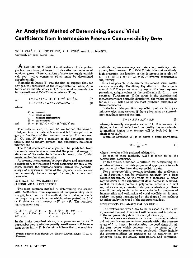
bilities a t pressures below the critical region for isotherms above the critical temperature. Table I gives the tempera- tures a t which isotherms were determined, the pressure range for each isotherm, the saturation pressure, and the number of experimental points available for each isotherm.

For each isotherm, the coefficients A , in Equation 4 were calculated by a least squares routine for k = 1, 2, 3, . . . , n - 1. The plots of 2 us. P for 2-methylbutane (9) indicate clearly that the slope and the curvature of each isotherm are negative over the entire range of pressures examined. As a result, any polynomial in which both the coefficients A 1 and A2 are not negative is not acceptable, because these

Table I. Temperature and Pressure Ranges of Compressibility Isotherms

Temp., Pressure Saturation No. of c. Rgnge, Atm. Pressure, Atm. Pointsa

50 0- 2.0 2.025 8 75 0- 3.9 3.983 14 100 0- 7.0 7.106 21 125 0-11.6 11.787 25 150 0-18.1 18.449 29

21 30

175 0-27.4 27.856 34 b

188.5 0-31.7 200 0-37.7

;Includes P = O.oooO,Z = 1.oooO. Critical temperature of 2-methylbutane is 187.8" C.

coefficients are related to the slope and the curvature of the isotherms as P approaches zero as follows:

A , = (az/ap)p,o 2~~ = (a'z/a P2)p - For the polynomials in which both A1 and A2 are negative, if their curvature is negative over the entire range of pressures, then their slopes are also negative over the same range. This follows from the fact that a polynomial is a single valued, continuous function.

SECOND VlRlAL COEFFICIENTS OF 2-METHYLBUTANE The order of the acceptable polynomials of 2 in terms of

P-i.e., those which describe the isotherm correctly as to slope and curvature-and their coefficients A , are given in Table 11. The negativity of the curvature of each polyno- mial was ascertained by examining its second derivative at regular intervals of 0.05 atm. from P = 0 up to the maximum pressure.

For each isotherm, the value of the coefficient A1 which occurs in the highest order acceptable polynomial was chosen to estimate the value of B', (B' = AIRT) , the second vinal coe5cient. The values of A I R T are given in Table 111.

In Table IV, a comparison is given between the percent- age residuals, (Zobd, - Zdcd,) lOO/Z,~., and the estimated maximum experimental errors (9) in determining the values

Temp., C , 50 75

100

125

150

175

188.5

200

75 125

175

188.5 200

k 1 1 2 4 5 1 2 3 1 2 4 6 8 1 2 4 1 2 4 6 8 1 2 4 6 1 2 4 6 8 9

5 6 8 6 8 6 6 8 9

Table II

A0

0.99960816 1.0028402 0.99952888 1.0000048 1.0000053 1.0047020 0.99881099 0.99988468 1.0072075 0.99771404 0.99991109 0.99997981 1.0000090 1.0115168 0.99598463 0.99933014 1.0231045 0.98970414 0.99736594 0.99949764 0.99986789 1.0296749 0.98926459 0.99808439 0.99987374 1.0298854 0.98801397 0.99716683 0.99966208 0.99999735 0.99998596

A ~ X 10' -32.081006 48.946756 197.36119 2.62241 39 17.580103 0.84133494 0.50098160 1.6646745 3.2172451

I - k

Coefficients A, of All Acceptable Polynomials Z = A,P' 1-0

A l x lo2 A ' X 10' A ~ X io5 -3.6584917 -2.9576883 -2.5324205 - 10.284228 - 2.5832263 -17.162174 63.049460 -2.5936475 -15.253042 50.754788 -2.4345525 - 1.9525196 - 2.1187441 - 2 . 0 5 5 ~ 9 4

-6.7251232 -0.81268160 -5.5814615

- . - - - - - - - -1.5245690 -4.6710511 -1.7231826 -1.1662607 -0.53093630 - 1.6854939 -7.2994107 28.261556 -1.7178162 -4.4384247 25.456424 -1.7781456 -1.1523503 -1.3474609

-3.6683986 -2.1188107 0.89982920

-1.6579654 -0.73059102 -3.4903931 -0.93372900 -5.4546598 3.4277563 - 1,1004047 - 3.7364872 6.5442843 - 1.1602931 -2.2314362 8.9339980 -1.5133786 -0.67228118 - 2.6236214 -0.87629795 -3.8069234 2.0012275 - 1.0405172 - 1.5722063 2.4066044 -1 41WM - . - -- - _-- - 0.56945833 -2.3164221 - 0.75532377 - 3.6593548 1.6565327 -0.91793592 - 1.9165886 2.2316467 -0.96914958 -0,34964810 0.9731 2090 -0.96204394 - 0.86846651 2.4121913

A s x 10' A , X io9 A 8 x 10"

-15.472657 -236.05385 149.84088 -386.36487 -0.40708731 -9.1037407 2.4096214 -2.5767082 - 0.11748380 -0.058531700 - 0.66552083 0.13397502 -0.10940662 - 1.3746704 0.32260754 -0.37977136

A ~ x lo6

- 113.65423 -80.423967

-1.1250019 -57.612598 - 96.395228

-0.72638324

-0.93467584 -6.3572541 -18.140016

-0.47588374 -2.2654993

- 0.32596987 -1.6306168 -2.1265863 -4.1217699

A ~ X 101'

1.6133517

344 JOURNAL OF CHEMICAL A N D ENGINEERING DATA

Table Ill.

Temp.,

Second Virial Coefficients of 2-Methylbutane -AIM', Liter/Gram Mole

c. Unweighted Weighted polynomials polynomials

50 0.9701 1126 0.97651470 75 0.74095477

100 0.64874715 0.65079210 125 0.56122395 ~~~

150 175 188.5 200

0.46786726 0.42668038 0.39416076 0.37351221

"Weighting not necessary.

0.48310445 0.41927100 0.39625464

Table IV. Comparison of Residuals and Experimental Errors

Residuals, % Unweighted Weighted Polynomials Polynomials Temp.,

O c. Av. Max. Av. Max. 50 0.04 0.08 0.04 0.10 75 0.05 0.13

100 0.03 0.09 0.03 0.09 ~ ~~ --.

125 0.03 0.06 150 0.05 0.12 0.05 0.13

175 0.02 0.08 0.04 0.27

Estd. M S .

Exptl. Error, %

0.15 0.15 0.25 0.25 0.30 0.30.

0.02 0.08 0.02 0.08 0.30' 188.5

0.01 0.04 O.3Ob 200 0.04 ( 0.10 0.65'

I 0.09 0.22 ( 0.09 0.22 ( 3.0

b 'At saturation. Below 27 atm. '27-37 atm.

ofZObsd. All the residuals are well within the limits of experimental error.

POLYNOMIALS CALCULATED FROM WEIGHTED DATA

In calculating the least squares fits for each isotherm, a value of 2 = 1.0000 a t P = 0.0000 was added to the experimental results, and was given a weight equal to the weight of each experimental data point. In the polynomials adopted to represent the compressibility, 2, over the pres- sure ranges examined, the values of the first terms (Ao) represent the estimates of the first virial coefficients. The fact that for some isotherms these values are not equal to 1.0000 will now be considered.

Deviation of A. from 1.0000 arises from either random

or systematic errors in the data. I t is possible to force the polynomial to go through 1.0000 a t zero pressure by weighting the point (0.0000, 1.0000) more than the experi- mental points, but it must be kept in mind that the second vinal coefficient is represented by the slope of the poly- nomial a t zero pressure. If the errors are random, then the data points fall on either side of the true isotherm, and forcing A0 to be 1.0000 will result in a slope which is valid for estimating the second vinal coefficient. However, if the errors are systematic, the data points fall mostly on one side of the isotherm, and forcing the polynomial to go through 1.0000 a t zero pressure will give an incorrect slope. In fact, if the compressibility data are known to contain systematic errors, the slope of a polynomial calculated with- out the addition of the point (0.0000, 1.0000) would give the better estimate of the second virial coefficient.

Inasmuch as no systematic errors were known to exist in the data, each highest order acceptable polynomial was forced through 1.0000 a t zero pressure. For the highest order polynomials a t each temperature in which A . was not equal to 1 .OOOO, increasing weighting factors were applied to the point 2 = 1.0000 a t P = 0,0000 and the least squares fits were recalculated. The resulting polynomials were then tested as to slope and curvature. In order not to reduce the influence of the experimental data points unduly, the smallest weighting factor which made A . = 1.0000 in the highest order acceptable polynomial was employed.

The coefficients of all the acceptable weighted polyno- mials are given in Table V, along with the order of the polynomials and the weighting factor employed in each case. In these polynomials, the coefficients Ao are equal to 1.0000, and the coefficients A , are those employed in estimating the second virial coetficients. Values of A I R T , the second virial coefficients estimated from the weighted polynomials, are given in Table 111.

Table IV gives the residuals of the weighted polyno- mials and the estimated maximum experimental errors. Again, the residuals are all within the limits of the experi- mental error.

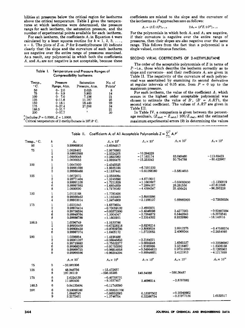
SMOOTHED VALUES OF SECOND VlRlAL COEFFICIENT

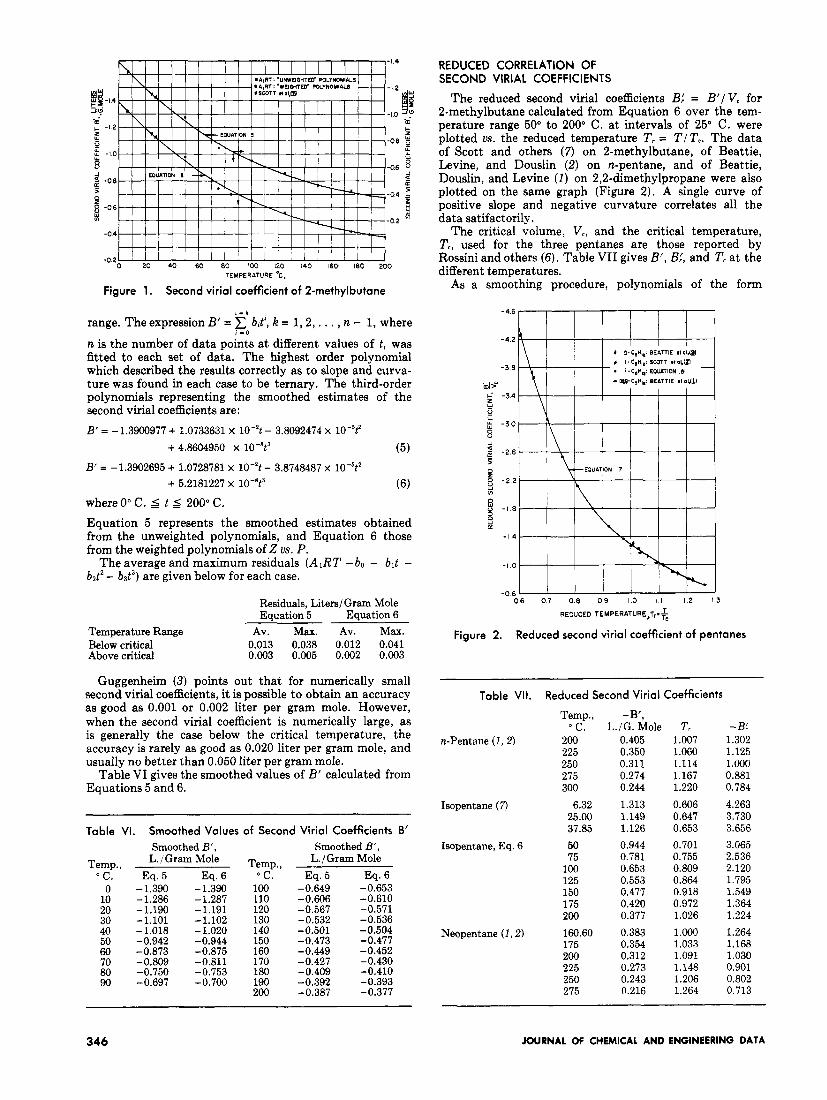
The estimates of the second virial coefficients obtained from both the weighted and weighted polynomials of 2 us. P (Table 111) were plotted against temperature. (Figure 1). The values reported by Scott and others (7) were also included to extend the temperature to 0" C.

A smooth curve of positive slope and negative curvature describes the results satifactorily over the 0" to 200" C.

8 - k

Table V. Coefficients A, of All Acceptable Weighted Polynomials Z = A,P1 2 = O

Temp., Weighting c. Factor k A0 A ~ x 10' A ~ X 10' A ~ X io5 A ~ X lo6 A 5 x lo7 AsX lo8

50 3.30 1 0.99995176 -3.6826404 100 1.66 1 1.0036497 -2.4100569

2 0.99932702 - 1.9833749 -6.3576637 3 0.99995098 -2.1254227 -0.62834810 -5.7301874

150 5.00 1 1.0036158 -1.7041281 2 0.99931067 -1.2397828 -3.2385870 4 0.99995720 -1.3913444 -1.2393085 0.23955280 -0.56099880

175 3.95 1 1.0111186 -1.5893103 2 0.99679988 -0.85158319 -3.1093830 4 0.99965329 -1.0450068 -3.9574719 2.6828610 -0.81171518 6 0.99995934 -1.1401444 -2.6318618 5.1786318 -5.5256232 2.3781652 -0.37945895

188.5 1.75 1 1.0219725 -1.4792729 2 0.99367784 -0.72782355 -2.4809787 4 0.99924043 -0.92019810 -3.3288370 1 BO41599 - 0.44852591 6 0.99995721 -1.0460447 -1.4515823 2.2867144 - 2.2057859 0.82681610 -0.1161 1221

~ ~~

VOL. 5, No. 3, JULY 1960 345

-I 4

-I 2

42 ia

-m. 'm c - 1 2 c z - 0 -08 E -

Y

Y B - I 0 -06

9 -08 c a 5

-04 > 9 8

0

-06

D - 0 2

-04

0 20 40 60 80 100 I20 140 160 180 200 TEMPERATURE %.

-0 2

Figure 1. Second virial coefficient of 2-methylbutane

I - I

range. The expression B' = bit', 12 = 1,2, . . . , n - 1, where

n is the number of data points a t different values of t , was fitted to each set of data. The highest order polynomial which described the results correctly as to slope and curva- ture was found in each case to be ternary. The third-order polynomials representing the smoothed estimates of the second vinal coefficients are:

'-0

B' = -1.3900977 + 1.0733631 x 10-*t - 3.8092474 x 10-5f

+ 4.8604950 x ( 5 )

+ 5.2181227 X 10-'t3 (6) where 0" C. 5 t 5 200" C. Equation 5 represents the smoothed estimates obtained from the unweighted polynomials, and Equation 6 those from the weighted polynomials of Z us. P.

The average and maximum residuals (AIRT -bo - blt - bzt2 - b3t3) are given below for each case.

B' = -1.3902695 + 1.0728781 x - 3.8748487 x 10-'t2

Residuals, Liters/ Gram Mole Equation 5 Equation 6

Temperature Range Av. Max. Av. Max. Below critical 0.013 0.038 0.012 0.041 Above critical 0.003 0.005 0.002 0.003

Guggenheim (3) points out that for numerically small second virial coefficients, it is possible to obtain an accuracy as good as 0.001 or 0.002 liter per gram mole. However, when the second virial coefficient is numerically large, as is generally the case below the critical temperature, the accuracy is rarely as good as 0.020 liter per gram mole, and usually no better than 0.050 liter per gram mole.

Table VI gives the smoothed values of B' calculated from Equations 5 and 6.

~~ ~

Table VI. Smoothed Values of Second Virial Coefficients 6' Smoothed B', Smoothed B', L./Gram Mole Temp., L./Gram Mole Temp.,

o C . Eq. 5 Eq. 6 " C . Eq.5 Eq. 6 ('I -1.390 -1.390 100 -0.649 -0.653

10 20 30 40 50 60 70 80 90

~

-1.286 -1.190 -1.101 - 1.018 -0.942 -0.873 -0.809 -0.750 -0.697

-i.i87 -1.191 -1.102 - 1.020 -0.944 -0.875 -0.811 -0.753 -0.700

110 120 130 140 150 160 170 180 190 200

-0.606 -0.567 -0.532 -0.501 -0.473 -0.449 -0,427 -0.409 -0.392 -0.387

-0.610 -0.571 -0.536 -0.504 -0.477 -0.452 -0.430 -0.410 -0.393 -0.377

346

REDUCED CORRELATION OF SECOND VlRlAL COEFFICIENTS

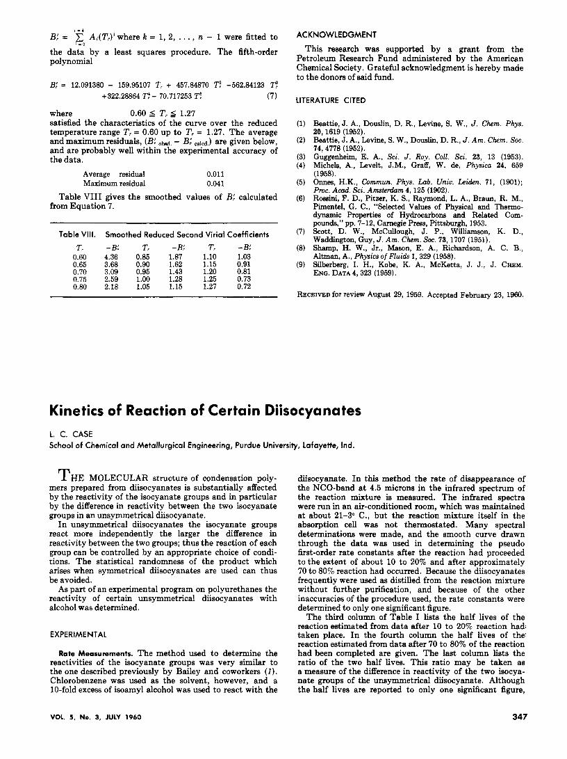
The reduced second virial coefficients B: = B' /V , for 2-methylbutane calculated from Equation 6 over the tem- perature range 50" to 200" C. a t intervals of 25" C. were plotted us. the reduced temperature T, = TIT,. The data of Scott and others (7) on 2-methylbutane, of Beattie, Levine, and Douslin (2) on n-pentane, and of Beattie, Douslin, and Levine (1) on 2,2-dimethylpropane were also plotted on the same graph (Figure 2) . A single curve of positive slope and negative curvature correlates all the data satifactorily.

The critical volume, V,, and the critical temperature, T,, used for the three pentanes are those reported by Rossini and others (6). Table VI1 gives B', B:, and T, at the different temperatures.

As a smoothing procedure, polynomials of the form

-4'6 m

- 2 6 > 0 8 - 2 2

n % - I 8

t: - I 4

-I 0

I I I I I 1 1 - 1 - 0 6 l I I I I I I I

0 6 07 0 8 09 10 I 1 1 2 13

REDUCED TEMPERATURE,T,+

Figure 2. Reduced second virial coefficient of pentanes

~ ~~

Table VII. Reduced Second Virial Coefficients

Temp., -B', " C . L./G. Mole T, - B:

n-Pentane ( I , 2 ) 200 0.405 1.007 1.302 225 0.350 1.060 1.125 250 0.311 1.114 1.OOO 275 0.274 1.167 0.881 300 0.244 1.220 0.784

Isopentane (7) 6.32 1.313 0.606 4.263 25.00 1.149 0.647 3.730 37.85 1.126 0.653 3.656

Isopentane, Eq. 6 50 0.944 0.701 3.065 75 0.781 0.755 2.536

100 0.653 0.809 2.120 125 0.553 0.864 1.795 150 0.477 0.918 1.549 175 0.420 0.972 1.364 200 0.377 1.026 1.224

Neopentane ( I , 2) 160.60 0.383 1.OOO 1.264 175 0.354 1.033 1.168 200 0.312 1.091 1.030 225 0.273 1.148 0.901 250 0.243 1.206 0.802 275 0.216 1.264 0.713

JOURNAL OF CHEMICAL AND ENGINEERING DATA

I - I

B: = C A,(T,)’where k = 1, 2, . . . , n - 1 were fitted to

the data by a least squares procedure. The fifth-order polynomial

I - 0

B: = 12.091380 - 159.95107 T, + 457.84870 !L? -562.84123 T: +322.28864 T: - 70.717253 T: (7)

where 0.60 5 T, 4 1.27 satisfied the characteristics of the curve over the reduced temperature range T, = 0.60 up to T, = 1.27. The average and maximum residuals, (B: ow. - B: cdcd.) are given below, and are probably well within the experimental accuracy of the data.

Average residual 0.011 Maximum residual 0.041

Table VI11 gives the smoothed values of B: calculated from Equation 7.

Table VIII. Smoothed Reduced Second Virial Coefficients

T, - B: T, - B: T, - B: 0.60 4.36 0.85 1.87 1.10 1.03 0.65 3.68 0.90 1.62 1.15 0.91 0.70 3.09 0.95 1.43 1.20 0.81 0.75 2.59 1.00 1.28 1.25 0.73 0.80 2.18 1.05 1.15 1.27 0.72

ACKNOWLEDGMENT

This research was supported by a grant from the Petroleum Research Fund administered by the American Chemical Society. Grateful acknowledgment is hereby made to the donors of said fund.

LITERATURE CITED

Beattie, J. A,, Douslin, D. R., Levine, S. W., J. Chem. Phys. 20,1619 (1952). Beattie, J. A., Levine, S. W., Douslin, D. R., J . Am. Chem. SOC. 74,4778 (1952). Guggenheim, E. A., Sci. J . Roy. Coll. Sci. 23, 13 (1953). Michels, A., Levelt, J.M., Graff, W. de, Physica 24, 659 (1958). h e s , H.K., Commun. Phys. Lab. Univ. Leiden. 71, (1901); Pmc. A d . Sci. Amsterdam 4, 125 (1902). Rossini, F. D., Pitzer, K. S., Raymond, L. A., Braun, R. M., Pimentel, G . C., “Selected Values of Physical and Thermo- dynamic Properties of Hydrocarbons and Related Com- pounds,” pp. 7-12, Carnegie Press, Pittsburgh, 1953. Scott, D. W., McCullough, J. P., Williamson, K. D., Waddington, Guy, J . Am. Chem. Soc. 73,1707 (1951). Shamp, H. W., Jr., Mason, E. A., Richardson, A. C. B., Altman, A,, Physicsof Fluids 1,329 (1958). Silberberg, I. H., Kobe, K. A., McKetta, J. J., J. CHEM. ENC. DATA 4,323 (1959).

RECEIVED for review August 29, 1959. Accepted February 23, 1960.

Kinetics of Reaction of Certain Diisocyanates

L. C. CASE School of Chemical and Metallurgical Engineering, Purdue University, Lafayette, Ind.

THE MOLECULAR structure of condensation poly- mers prepared from diisocyanates is substantially affected by the reactivity of the isocyanate groups and in particular by the difference in reactivity between the two isocyanate groups in an unsymmetrical diisocyanate.

In unsymmetrical diisocyanates the isocyanate groups react more independently the larger the difference in reactivity between the two groups; thus the reaction of each group can be controlled by an appropriate choice of condi- tions. The statistical randomness of the product which arises when symmetrical diisocyanates are used can thus be avoided.

As part of an experimental program on polyurethanes the reactivity of certain unsymmetrical diisocyanates with alcohol was determined.

EXPERIMENTAL

Rate Measurements. The method used to determine the reactivities of the isocyanate groups was very similar to the one described previously by Bailey and coworkers (I). Chlorobenzene was used as the solvent, however, and a 10-fold excess of isoamyl alcohol was used to react with the

diisocyanate. In this method the rate of disappearance of the NCO-band at 4.5 microns in the infrared spectrum of the reaction mixture is measured. The infrared spectra were run in an air-conditioned room, which was maintained at about 21-3” C., but the reaction mixture itself in the absorption cell was not thermostated. Many spectral determinations were made, and the smooth curve drawn through the data was used in determining the pseudo first-order rate constants after the reaction had proceeded to the extent of about 10 to 20% and after approximately 70 to 80% reaction had occurred. Because the diisocyanates frequently were used as distilled from the reaction mixture without further purification, and because of the other inaccuracies of the procedure used, the rate constants were determined to only one significant figure.

The third column of Table I lists the half lives of the reaction estimated from data after 10 to 20% reaction had, taken place. In the fourth column the half lives of the reaction estimated from data after 70 to 80% of the reaction had been completed are given. The last column lists the ratio of the two half lives. This ratio may be taken as a measure of the difference in reactivity of the two isocya- nate groups of the unsymmetrical diisocyanate. Although the half lives are reported to only one significant figure,

VOL. 5, No. 3, JULY 1960 347