An adaptive mesh refinement procedure de Urquijo …...An adaptive mesh refinement procedure for shape optimal design J. Canales, J.A. Tarrago, A. Hernandez Department of Mechanical

An adaptive mesh refinement procedure

for shape optimal design

J. Canales, J.A. Tarrago, A. Hernandez

Department of Mechanical Engineering, Faculty of

Engineering, University of the Basque Country, Alda.

de Urquijo s/n. 4̂ 013 Bilbao, Spain

ABSTRACT

In this paper we present a procedure for automatic mesh generation specificallycreated for shape optimal design problems. This procedure is implemented as amodule in a general system for shape optimal design of linear elastic structures.The module provides the mesh generation and its adaptive refinement. It worksin a whole automatic way. The input is the geometric definition and the result isthe refined mesh. First a basic mesh is generated using conformal mappingconcepts and second the basic mesh is refined using an error estimator based inthe strain energy density function and -h and -p remeshing techniques. Somesamples of shape optimal design solved with these concepts are presented.

INTRODUCTION

Shape Optimal Design has been studied in the last twenty years. Since the firstworks published by Zienkiewicz and Campbell [1] up to now, a lot of progresshas been made, making possible the implementation of these optimizationtechniques in the Computer Aided Engineering Systems (CAE). However, thereare still few authors who concentrate in the development of integratedapproaches for shape optimal design systems [2].

Some software distributors have introduced optimal design modules in theirgeneral-purpose FE programs. In fact, more than acceptable results have beenobtained for solving the so called size optimization problems. Nevertheless,shape optimal design brings in new difficulties which makes it much harder tointegrate all the different techniques involved in the structural synthesis. Forexample, in the problems of size optimal design, once the sensitivities have beencalculated, the modification of the design is quite simple and the corresponding

Transactions on the Built Environment vol 2, © 1993 WIT Press, www.witpress.com, ISSN 1743-3509

124 Optimization of Structural Systems

variations in the FE model are straightforward. The process becomescomplicated in the problems of shape optimal design in which the variations inthe shape of the design imply significant changes in the corresponding FE modeland as the shape is iteratively changed, the FE mesh gets increasingly distorted,and also the way that the piece works changes. That needs to be controlled sothat finite element analysis and response calculations are reliable. Further,adaptive meshing allows for larger shape changes to occur and ensure that theoptimization process terminates successfully. So that the practical exercise ofshape optimization demands the integration, through a unified approach, of thegeometric preprocessing modules, FE analysis and numerical techniques ofoptimization.

In this paper we shall concentrate in the Adaptive Meshing module that hasbeen implemented in CODISYS (Computer Optimal Design Integrated System),a system that has been developed in the Mechanical Engineering Department ofthe Basque Country University [3]. This system allows for the automatization ofthe shape optimal design cycle of two-dimensional elastic structures andaxisymmetrical space structures.

Although much work has been done on adaptivity in purely FE applications,implementing such capabilities in shape optimization deserves further attentionand is very important for developing a robust program. The adaptive meshingmodule that has been implemented, provides the mesh generation and itsadaptive refinement. It works in a whole automatic way. The input is thegeometric definition and the result is the refined mesh. First a basic mesh isgenerated using conformal mapping concepts and second the basic mesh isrefined using an error estimator based in the strain energy density function.

GEOMETRICAL REPRESENTATION

The adequate election of a geometrical representation method of the designvariables is of fundamental importance in order to achieve an automatic designcycle. On the right choices depend such important matters as:

— The degree of difficulty involved in the numerical solving of the resultingproblem. This problem has a non-linear formulation, more or less markeddepending on the chosen variables. The fewer design variables the better,because superfluous variables further complicate the problem without anappreciate improvement in the results.

— The quality of the results, that is the obtaining of regular, real and practicalshapes for the boundaries, in the most automatic way possible, that is,avoiding having recourse to further restrictions in the optimization;

— And the updating of the FE mesh in order to avoid a loss of accuracy in theanalysis, as the shape of the boundaries keeps varying;


Optimization of Structural Systems 125

The procedure chosen in CODISYS for the Geometrical Representation isthat of the Elements of Design. The modifications suggested by Braibant andFleury [4,5] have been incorporated. These are based on the use, for thedescription of boundaries and areas, of the blending functions and the usualCAD procedures as well as some additional modifications. This procedure hasbeen described further on a previous work [6].

Based on these premises a formulation has been proposed for theGeometrical Representation that distinguishes three models: the Model of theGeometrical Representation of the structure itself, and the Models of Designand Analysis of the structure. For the description of the Geometrical Model -which is strictly limited to defining the geometry of a piece-, use has been madeof the usual CAD functions and techniques for the interactive generation ofcurves [7,8].

A Y

FIRST PARTITION^ LEVEL

I- Design Dement2,3,4. Fixed Subreglons(1). Moving Boundary

SECOND PARTITIONFinite Elements

LEVEL

GEOMETRIC MODEL DESIGN MODEL ANALYSIS MODEL

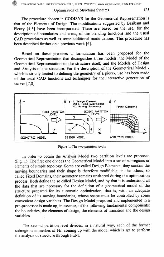
Figure 1. The two partition levels

In order to obtain the Analysis Model two partition levels are proposed(Fig. 1). The first one divides the Geometrical Model into a set of subregions orelements of simple topology. Some are called Design Elements: they contain themoving boundaries and their shape is therefore modifiable; in the others, socalled Fixed Domains, their geometry remains unaltered during the optimizationprocess. Both define the so called Design Model, and by that it is understood allthe data that are necessary for the definition of a geometrical model of thestructure prepared for its automatic optimization, that is, with an adequatedefinition of its moving boundaries, whose shape must be controlled by someconvenient design variables. The Design Model proposed and implemented in apre-processor is made up, in essence, of the following fundamental components:the boundaries, the elements of design, the elements of transition and the designvariables.

The second partition level divides, in a natural way, each of the formersubregions in meshes of FE, coming up with the model which is apt to performthe analysis of structure through FEM.



GENERATION AND UPDATING OF THE MESH OF FINITE ELEMENTS.

The module of mesh generation is of great importance in the general algorithm.The greater or lesser facility with which the integration of the rest of themodules can be carried out, depends on the degree of sophistication of the meshgenerator. An algorithm of mesh generation which is adequate to the problemsof shape optimal design should have the following features:

— It must be efficient and totally automatic, ensuring the integrity of the meshand therefore the validity of the analysis throughout the iterative process;

— It must be able to generate meshes for any geometry without manualintervention;

— The amount of data put into the mesh generator must be minimum;— It must have the capacity of generating adaptive meshes, not only to the

variation in the geometry but also to variations in the way the structureworks as the design progresses (e.g. zones of concentration of stresses thatappear, disappear or change position).

Following these ideas a module has been implemented in CODISYS ofautomatic mesh generation which generates the mesh in a completely automaticway, with no intervention by the user, in a relatively short time. It works in twosteps:

r) Basic mesh generation with a transfmite interpolation technique.2°) Adaptive mesh refinement of the basic mesh with an error estimator based

on the Strain Energy Density.

Basic Mesh GenerationIn order to generate the basic FE mesh from the Design Model, the transfmiteinterpolation technique has been chosen, because it can be understood as anatural extension of the methods used for the definition of superficial elements[9]. Through this technique a mesh of points is created. In this mesh, the FE aredefined, getting in this way the second partition level on the Geometric Modeland obtaining the FE Analysis Model, after imposing the applied loads and theboundary conditions.

These transformations set up an explicit relation which allows to determinethe coordinates of any point (e.g. a FE node) inside the design element or on itsboundary lines, depending on the actual position of the control points whichdefine that design element. Moreover they provide a procedure for generationand automatic updating of the FE mesh. In the design elements, this mesh isupdated in each iteration, according to the results obtained in the optimization.Inside the fixed subregions, the user can define the most suitable mesh whichwill remain unaltered during the whole process.



Adaptive Mesh RefinementThe aim of the adaptive mesh refinement module is to provide a mesh thatminimizes the discretization error. It is an adaptive scheme based on the strainenergy density (SED), that includes -h, -p and -hp refinements.

The starting point for the error analysis is the strain energy density, whoseexpression at any point in the domain is

y(x,y) = -u^

where u is the nodal displacement vector (computed in the basic mesh); B isthe strain-displacement matrix, and D is the elastic modulus matrix

The strain energy is a scalar magnitude that depends on the interpolationfunctions which, as is already known, depend in turn on the element beingconsidered and on the coordinates of the specific point. In a FE representation,matrix B and matrix N of the interpolation functions are related through the

differential operator 3 in the form

which means in our case that the SED is one degree of differentiation lowerthan the displacement interpolation functions. The importance of this fact will be

shown later.

If the SED expression is compared with the one of the stresses, they look

similar

O = DBu (3)

Both include the Bu product and their units are the same. The difference lies inthe fact that the stress field is a tensor while the SED field is a scalar magnitude.This shows the first advantage of SED: it is a single value and therefore doesnot depend on the coordinate system being considered.

Error Analysis The shape of the SED surface coming from the FE analysis isdiscontinuous, made up of steps. These discontinuities establish a differencebetween the SED coming from the FE analysis and the exact value. If theproblem is solved analytically a continuous density field will be obtained.Intuitively, the smaller the discontinuities of the discrete field, the more accurateis the solution. If by starting from the values of the discrete field, a smoothed(continuous) field could be obtained which fulfills a number of physical



conditions then it is obvious that this smooth field from the SED is closer to thetrue field. In order to obtain this smooth field nodal values have to be used.

Let y be the discontinuous strain energy density field and y~ its smoothed

field. Y is the vector storing the nodal values of the discontinuous surface, and

*P stores the same values for the smoothed field. In order to interpolate the

nodal values of the smoothed field the same functions used for the interpolation

of displacements will be employed. The smoothed field is then written

V/=NY* (4)

The definition of the estimator is straightforward. The estimator of thedensity error is the difference in absolute value between the smoothed field andthe discontinuous field

*-y| (5)

The error in the energetic norm is straightforward. This is the first

advantage of the use of densities: all that needs to be done is to integrate e^

along the domain so as to obtain the error in the energetic norm. The rules of

integration of the stiffness matrix are also valid for the calculation of the error

integrals, since the interpolation functions are the same. For one element, the

energy error is

14 = k̂ (6)

Adding up the contribution of ail the elements, the energy error along thewhole of the domain is obtained

In order to obtain the percentage of error(̂ ), one of the most commonexpressions has been adopted [10]

IMIc

where U is the strain energy of the FE model.



Refinement procedure During the last few years, important advances have beenmade in the development of-hp remeshing techniques [11,12,13]. However,those techniques are still very complicated and are thus only applicable to simplecases. At the same time, some authors have been trying to simplify thetechnique, developing algorithms based on simple and intuitive ideas [14,15].The results are very good and although it means an important advance withregard to the present algorithms, these new procedures have their limitations.

In very detailed comparative analyses found in the references [16], it can benoticed the different quality performance between the quadrilateral linear andtriangular linear elements. In meshes that include both types of elements, thetriangular elements introduce higher errors. What can even happen is that, whendividing a quadrilateral element into four triangles, the error does not decrease,but actually increases. The simplest way to improve the performance of a linearelement is to transform it into a quadratic element. This is the method used inthis work: a quasi-optimal mesh of linear elements is first obtained and then thequality of the mesh is regularized by introducing a -p refinement. The adequacyof this method will be shown through examples.

After performing an analysis of error, the error by element in the energetic

norm is available. For the i element, the energetic norm error is \\e\\ ̂.. When

optimizing the discretization error, the target is to distribute the error uniformly

over the whole of the domain. That means that the \\e\\ ̂ value must be similar in

all the elements. Let us assume that one mesh with such requirements is

available and, besides, the size of the elements is very different. If two elements

of very different size are compared, clearly the smaller element is of lower

quality than the bigger one. It would be enough to see the shape of the energydensity surface to notice it. In all the points of the smallest element, the density

error would be higher than in the other element. Intuitively it is seen the need of

untying the volume from the measure of the quality of the element. The quality

is related to the energy density error, that can change significantly inside the

element. Since we are interested in the values for each element, the best

approach is the mean value of the strain energy density error. In this case

(9)

Of course, (p- has all the limitations of average values: for very large

elements the mean value can be very different from the values at certain

locations in the same element. Anyway cp. it is always a good measure. Let /?, be



the size of the initial element and h^- the size needed to obtain a prescribed

error. Applying convergence concepts, it is known that [15]

(10)

where p is the order of the polynomial used to interpolate the displacements andA the singularities intensity factor. Now it is easy to deduce the size of meshthat is necessary to obtain a specific error.

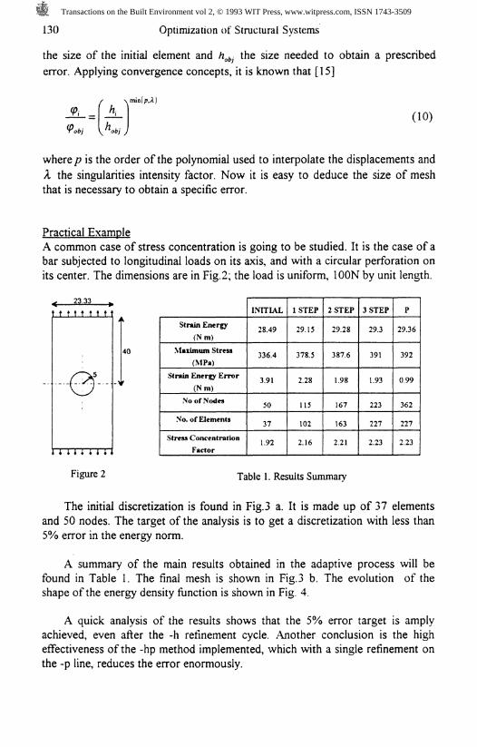
Practical ExampleA common case of stress concentration is going to be studied. It is the case of abar subjected to longitudinal loads on its axis, and with a circular perforation onits center. The dimensions are in Fig.2; the load is uniform, 100N by unit length.

23.33-ULLULUJ

40

Strain Energy(Nm)

Maximum Stress(MPa)

Strain Energy Error(Nm)

No of Nodes

No. of Elements

Stress ConcentrationFactor

INITIAL

28.49

336.4

3.91

50

37

1.92

1STEP

29.15

378.5

2.28

115

102

2.16

2 STEP

29.28

387.6

1.98

167

163

2.21

3 STEP

29.3

391

1.93

223

227

2.23

P

29.36

392

0.99

362

227

2.23

Figure 2 Table 1. Results Summary

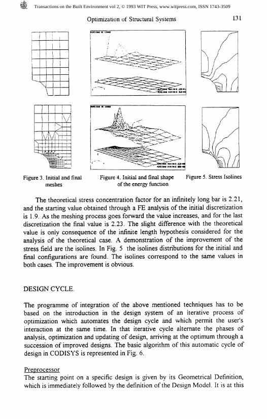
The initial discretization is found in Fig.3 a. It is made up of 37 elementsand 50 nodes. The target of the analysis is to get a discretization with less than5% error in the energy norm.

A summary of the main results obtained in the adaptive process will befound in Table 1. The final mesh is shown in Fig.3 b. The evolution of theshape of the energy density function is shown in Fig. 4.

A quick analysis of the results shows that the 5% error target is amplyachieved, even after the -h refinement cycle. Another conclusion is the higheffectiveness of the -hp method implemented, which with a single refinement onthe -p line, reduces the error enormously.



Figure 3. Initial and final Figure 4. Initial and final shape Figure 5. Stress Isolinesmeshes of the energy function

The theoretical stress concentration factor for an infinitely long bar is 2.21,and the starting value obtained through a FE analysis of the initial discretizationis 1.9. As the meshing process goes forward the value increases, and for the lastdiscretization the final value is 2.23. The slight difference with the theoreticalvalue is only consequence of the infinite length hypothesis considered for theanalysis of the theoretical case. A demonstration of the improvement of thestress field are the isolines. In Fig. 5 the isolines distributions for the initial andfinal configurations are found. The isolines correspond to the same values inboth cases. The improvement is obvious.

DESIGN CYCLE.

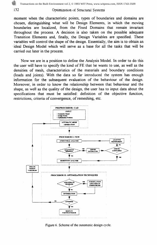
The programme of integration of the above mentioned techniques has to bebased on the introduction in the design system of an iterative process ofoptimization which automates the design cycle and which permit the user'sinteraction at the same time. In that iterative cycle alternate the phases ofanalysis, optimization and updating of design, arriving at the optimum through asuccession of improved designs. The basic algorithm of this automatic cycle ofdesign in CODISYS is represented in Fig. 6.

PreprocessorThe starting point on a specific design is given by its Geometrical Definition,which is immediately followed by the definition of the Design Model. It is at this



moment when the characteristic points, types of boundaries and domains arechosen, distinguishing what will be Design Elements, in which the movingboundaries are localized, from the Fixed Domains that remain invariantthroughout the process. A decision is also taken on the possible adequateTransition Elements and, finally, the Design Variables are specified. Thesevariables will control the shape of the design. Essentially, the aim is to obtain anideal Design Model which will serve as a base for all the tasks that will becarried out later in the process.

Now we are in a position to define the Analysis Model. In order to do thisthe user will have to specify the kind of FE that he wants to use, as well as thedensities of mesh, characteristics of the materials and boundary conditions(loads and joints). With the data so far introduced the system has enoughinformation for the subsequent evaluation of the behaviour of the design.Moreover, in order to know the relationship between that behaviour and theshape, as well as the quality of the design, the user has to input data about thespecifications that must be satisfied: definition of the objective function,restrictions, criteria of convergence, ofremeshing, etc.

PREPROCESSOR: CAD

Figure 6. Scheme of the automatic design cycle.



Processor I: FEMThe next stage involves the Module of Mesh Generation. Its function consists inconverting automatically the Design Model defined by the user into an AnalysisModel. The Analysis Model is immediately evaluated by the correspondingmodule, calculating the values of the suitable state variables (displacements,stresses, etc.), as well as the values of the specifications (objective function andrestrictions). On the basis of the results of the analysis and of the criterion ofremeshing previously defined, the Control Module makes the decision tocontinue the process transferring it directly to the Sensitivity Analysis Module,with or without a previous call to the Remeshing Module.

The Sensitivity Analysis being done, the derivatives of the objectivefunction and the restrictions with respect to the design variables provide theuser with valuable information about the behavioural tendency of the system.

The module implemented in CODISYS for the sensitivity analysis uses thewell-known semi-analytical method. Although some authors have questionedthe accuracy of the method for a certain kind of element [17] and forcomponents with a poor FE meshing, if the analysis model is sufficiently good -and this can be achieved with the adaptive mesh refinement techniques, as isdone in CODISYS- then it has been sufficiently proven that the semi-analyticalmethod is perfectly valid for many types of elements and for a wide range ofproblems [18]. Besides, it constitutes an adequate compromise between ease ofimplementation and the computational effort involved in the calculation.

Processor II: optimization techniquesFinally the Control Module transfers the design process to the Optimizer, whichperforms the opportune modifications in the Design Variables. Thesemodifications are transmitted to the Design Model, finishing a complete cycle ofShape Optimal Design.

The structural shape optimization problems are typically non-linearmathematical problems to which standard minimization techniques can beapplied. And so, the first and widely used approach to solve them is based onjoining together a general purpose method of mathematical programming (suchas gradient projection methods or the feasible directions method) and a FEpackage which may be able to perform the sensitivity analysis required in orderto solve the problem. This procedure could be called the "Direct Method".

The essential difficulty in applying this method for solving the problem liesin the implicit character of the constraint functions. Since the optimizationprocess is of an iterative nature, it will generally be necessary to make manyreanalyses of the structure before finding an acceptable solution.



In order to overcome these limitations, a considerable research effort hasbeen made in the last few years in order to develop new procedures based onthe approximation concept. Basically this consists in substituting for the originaloptimization problem a sequence of explicit approximate subproblems with asimple algebraic structure. Each subproblem is generated through a Taylorseries expansion, both of the function and of the constraints, in terms of someintermediate linearization variables. Then it is solved by means of a procedure ofmathematical programming.

Both approaches have been implemented in the CODISYS optimizationmodule, in such a way that the user can choose the approach he deems mostsuited to his specific problem of shape optimization.

EXAMPLES

Many practical problems have been solved with CODISYS to validate it [3].Here we present two of them to illustrate the description of the System.

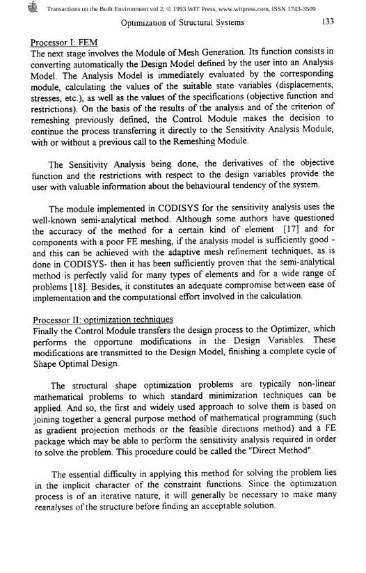
Optimization of a hole in a biaxial stress fieldThis example has been used as a typical key test-case to validate CODISYS.The plate with a hole is loaded with a combinedtension in two perpendicular directions (Fig. 7).The applied stress in the x-direction is twice that inthe ̂ -direction. The problem is to determine theshape of the hole for which the tangential stressesaround the hole are uniform. It can be proven thatthe shape with this property is an ellipse, with itsaxis ratio equal to the ratio of the applied tensilestress (0.5 in this case), and that is the solutionthat CODISYS gives.

j

F

P t t t t*t t t 1

o

1 1 1 1 1 1 1 1

igure 7. Plate with a

-o.

hole

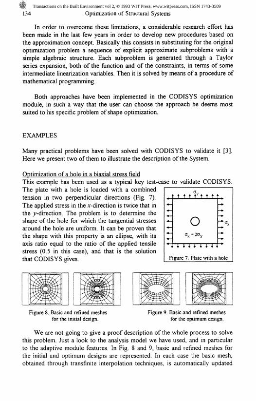
Figure 8. Basic and refined meshesfor the initial design.

Figure 9. Basic and refined meshesfor the optimum design.

We are not going to give a proof description of the whole process to solvethis problem. Just a look to the analysis model we have used, and in particularto the adaptive module features. In Fig. 8 and 9, basic and refined meshes forthe initial and optimum designs are represented. In each case the basic mesh,obtained through transfinite interpolation techniques, is automatically updated



according to the change in the boundary of the hole. For the initial design, stressconcentrations occur at the boundary of the hole, and the adaptive module givesa refinement area where it's necessary. For the optimum design, as the tangentialstresses are uniform (i.e., stress isolines round parallel to the shape of the hole),the refinement area is located round the hole. The module of mesh generationgives in this way, automatically, the optimum mesh in each intermediate design.

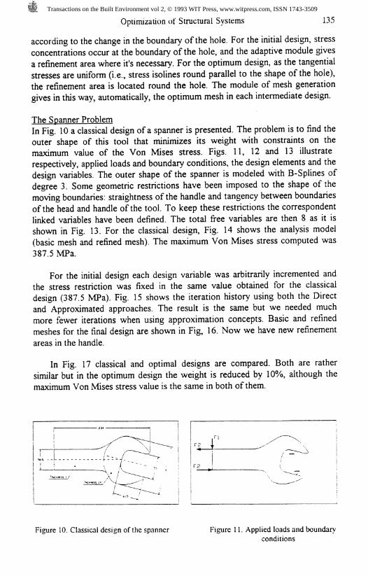
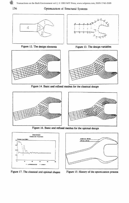
The Spanner ProblemIn Fig. 10 a classical design of a spanner is presented. The problem is to find theouter shape of this tool that minimizes its weight with constraints on themaximum value of the Von Mises stress. Figs. 11, 12 and 13 illustraterespectively, applied loads and boundary conditions, the design elements and thedesign variables. The outer shape of the spanner is modeled with B-Splines ofdegree 3. Some geometric restrictions have been imposed to the shape of themoving boundaries: straightness of the handle and tangency between boundariesof the head and handle of the tool. To keep these restrictions the correspondentlinked variables have been defined. The total free variables are then 8 as it isshown in Fig. 13. For the classical design, Fig. 14 shows the analysis model(basic mesh and refined mesh). The maximum Von Mises stress computed was387.5 MPa.

For the initial design each design variable was arbitrarily incremented andthe stress restriction was fixed in the same value obtained for the classicaldesign (387.5 MPa). Fig. 15 shows the iteration history using both the Directand Approximated approaches. The result is the same but we needed muchmore fewer iterations when using approximation concepts. Basic and refinedmeshes for the final design are shown in Fig, 16. Now we have new refinementareas in the handle.

In Fig. 17 classical and optimal designs are compared. Both are rathersimilar but in the optimum design the weight is reduced by 10%, although themaximum Von Mises stress value is the same in both of them.

Figure 10. Classical design of the spanner Figure 11. Applied loads and boundaryconditions



Figure 12. The design elements Figure 13. The design variables

Figure 14. Basic and refined meshes for the classical design

Figure 16. Basic and refined meshes for the optimal design

SPANNERObMcliv* FunctionCIXCICM. DUTCH

Figure 17. The classical and optimal shapes Figure 15. History of the optimization process



CONCLUSIONS

In this paper a procedure to ensure the accuracy of FE analysis, in shape optimalproblems has been proposed. An error analysis and adaptive meshing moduleshave been implemented in a general System for Structural Optimization. By thisprocedure, automatic and efficient mesh generation has been achieved. Theprocedure has been validated through its application to many practicalexamples.

Acknowledgments. - This research was partially supported by the grant UPV145.345-EA180/92 from Universidad del Pais Vasco, for which the authorsgratefully acknowledge.

REFERENCES

1. O. C. Zienkiewicz and J. S. Campbell, Shape Optimization and SequentialLinear Programming. In Optimum Structural Design (Edited by R. H.Gallagher and 0. C. Zienkiewicz), pp. 109-126, John Wiley (1973).

2. Y. Ding, Shape. Optimization of Structures: A Literature Survey. Comput.Struct. 24, 985-1004(1986)

3. J. Canales, Integration de las Tecnicas de CAD, Analisis de Estructuras yOptimization en un Sistema de Diseno Automatico de Estructuras. TesisDoctoral, Departamento de Ingenieria Mecanica, Universidad del PaisVasco, Bilbao, (1992).

3. H. Iman, Three Dimensional Shape Optimization. Int. J. Numer. Meth.Engng. 18, 661-673, (1982).

4. V. Braibant and C. Fleury, Shape Optimal Design using B-Splines. Comp.Meth. Appl. Mech. Engng. 44, 247-267, (1984).

5. C. Fleury and V. Braibant, Structural Synthesis: Toward a Reliable CADTool. Proc. from NATO /NASA/NSF/USAF AS! on Computer AidedOptimal Design: Structural and Mechanical Systems, Vol. 3, pp. 137-155,Troia, Portugal, (1986).

6. A. Arias, J. Canales and J.A. Tarrago, A Parametric Model of StructuresRepresentation and its integration in a Shape Optimal Design Procedure. InOptimization of Structural Systems and Industrila Aplications (Ed. by C.A:Brebbia and S. Hernandez), pp. 401-412, Elsevier Applied Science, 1991.

7. S. A. Coons, Modification of the Shape of Piecewise Curves. Comput.AidedDes. 9, 178-180, (1977).

8. F. Yamaguchi, Curces and Surfaces in Computer Aided Geometric Desig?i,Springer-Verlag, Berlin. Heidelberg, (1988).



9. C. A. Hall, Transfinite Interpolation and Applications to EngineeringProblems. In Theory of Approximation, Academic Press, (1976).

10. I. Babuska and W. C. Rheinboldt, A Posteriori Error Estimates for theFinite Element Method, Int. J. Numer. Meth. Engng. 12, 1597-1615,(1978).

11. I. Babuska, D. W. Kelly, S. R. Gago and O C. Zienkiewicz, A PosterioriError Analysis and Adaptative Processes in the Finite Element Method -Part I: Error Analysis. Int. J. Numer. Meth. Engng. 19, 1593-1619, (1983).

12. I. Babuska, D. W. Kelly, S. R. Gago and O. C. Zienkiewicz, A PosterioriError Analysis and Adaptative Processes in the Finite Element Method -Part II: Adaptative Mesh Refinement. Int. J. Numer. Meth. Engng. 19,1621-1656, (1983).

13. L. Demkowicz, J. T. Oden, W. Rachowicz and O Hardy, Toward anUniversal h-p Adaptive Finite Element Strategy. Comp. Meth. Appl. Mech.Engng. 77, 79-112, (1989).

14. J. J. Rencis, T. J. Urekew, K.-Y. Jong, R. Kirk and P. Federico, APosteriori Error Estimation for the Finite Element and Boundary ElementMethods. Comput. Struct. 37, 103-117, (1990).

15. O. C. Zienkiewicz, J. Z Zhu and N. G. Gong, Effective and Practical h-pVersion Adaptive Analysis Procedures for the Finite Element Method. Int.J. Numer. Meth. Engng. 28, 879-891, (1989).

16. R. Aviles, F. Viadero and A. Hernandez, A New Approach of FiniteElement Analysis Based on Error Estimators and an Adaptive Meshing.Report SA-142, Department of Mechanical Engineering, University of theBasque Country, Bilbao, (1990).

17. B. Barthelemy and R. T. Haftka, Accuracy Analysis of the Semi-AnalyticalMethod for Shape Sensitivity Calculation. Mech. Struct. Mach. 18, No. 3,407-432, (1990).

18. J. Rasmussen, E. Lund and T. Birker,Collection of Examples - CAOSOptimization System. 3rd Edn. Special Report No. 13, Institute ofMechanical Engineering, Aalborg University, (1992).


Documents

An adaptive mesh refinement procedure de Urquijo …...An adaptive mesh refinement procedure for shape optimal design J. Canales, J.A. Tarrago, A. Hernandez Department of Mechanical