AMERICAN

Journal of EpidemiologyFormerly AMERICAN JOURNAL OF HYGIENE

O 1977 by Thfi Johns Hopkins University School of Hygiene and Public Health

VOL. 106 AUGUST, 1977 NO. 2

Reviews and Commentary

A COMMENTARY ON THE MECHANICAL ANALOGUE TO THE REED-FROSTEPIDEMIC MODEL1

PAUL E. M. FINE1

Recent years have witnessed a consider-able increase in the development and useof mathematical and computer-basedmodels in infectious disease epidemiology.As a measure of this increase, Bailey (1)finds that the literature in this field hasgrown at a greater-than-exponential rateover the past two decades/ilthough onemay suspect that some of the publishedmodels have greater value as exercises inmathematics than as contributions to "realdisease" epidemiology, this is certainly nottrue of all of them; and many examples canbe cited of major contributions of mathe-matical models in revealing relationshipsunderlying complex epidemiologic phe-nomena, in hypothesis testing, and in the

1 From the Department of Biomedical and Envi-ronmental Health Sciences, School of Public Health,University of California, Berkeley.

This research was sponsored in part by GeneralResearch Support Grant 5-SO1-RR-05441 from theNational Institutes of Health.

1 Present address (for reprint requests): Ross In-stitute, School of Hygiene and Tropical Medicine,Keppel Street, London WC1, England.

This commentary is dedicated to Lowell Reed, toWade Hampton Frost and to the many other work-ers who have taught and published on this ingeniousmodel. The author is especially indebted to Dr. ChinLong Chiang for his encouragement and suggestionsin the preparation of this paper. Drs. Lola Elveback,Abraham M. Lilienfeld, Margaret Merrell andPhilip E. Sartwell also made helpful comments onthe manuscript.

rational formulation of public health pol-icy (1-4).

A further motive for the development ofmodels, and one which is sometimes over-looked, relates to their usefulness in class-room teaching. Indeed, it might even beargued that it is through this medium thatmodels have had their greatest impactupon the practice of epidemiology today. Itis probable that discussions of Muench's(5) catalytic models (especially at HarvardUniversity) and of Macdonald's (6) malariaequations (especially at the School of Hy-giene and Tropical Medicine in London)have been of major and enduring value tomany epidemiologists and public healthofficers, by introducing them clearly andforcefully to the quantitative subtleties ofepidemiologic processes. In this context, itis certain that no epidemiologic model hasenjoyed such widespread and lasting suc-cess in the teaching milieu as has thatoriginally developed at the Johns HopkinsUniversity by Wade Hampton Frost andLowell Reed, and which has come to beknown familiarly as the Reed-Frost model.

HISTORY OF THE REED-FROST MODEL

The story of the development of theReed-Frost model is both well and illknown. Though mentioned by Frost in aCutter lecture at Harvard in 1928, the

87

88 PAUL E. M FINE

model was never discussed in publicationsby its authors (7, 8). It is indeed ironic thatone of the more fertile ideas in twentiethcentury epidemiology shduld have beenconsidered by its authors as "too slight acontribution" for publication (9). But otherworkers (beginning with Zinsser and Wil-son:, in 1932) were impressed with themodel's potential usefulness for the inves-tigation of a variety of epidemiologic prob-lems. And it has since served as the basisof several important contributions, nota-bly by Elveback, Fox, and their colleagues(10, 11).

The beauty and strength of the Reed-Frost model lie in the simplicity and versa-tility of its algebraic formulation. The easewith which it is converted from determin-istic to stochastic form makes it ideal inthe context of teaching biomedical stu-dents, for whom stochastic theory may ap-pear somewhat threatening. Indeed, it iswith reference to this quality of theirmodel that Reed and Frost showed a spe-cial streak of their genii, in the develop-ment of a mechanical analogue to illus-trate the model's stochastic properties.

This mechanical model—based upon theprobabilists' traditional container full ofcolored balls-was developed at JohnsHopkins about 1930, and has since beenused in teaching laboratories in many in-stitutions both in the United States andabroad. Invented before the age of com-puters, this apparatus probably providedthe first technique for the stochastic simu-lation of epidemiologic phenomena withnon-biological material (we recall thatthere was considerable interest in animal-model "experimental epidemiology" atthat time in history). The mechanicalmodel has undoubtedly undergone trans-formations in its passage from one institu-tion to another; but none of these transfor-mations — let alone the basic model itself—has ever been fully described in publica-tion. This is surprising, as the relationshipbetween the algebraic formulation and themechanical analogue of the Reed-Frost

model is both interesting and subtle. Someaspects of this relationship may be over-looked in the epidemiology classroom; butothers frequently arise in discussion of themodel's properties. It then becomes of in-terest to explore different methods of treat-ing the relationship between the algebraicand mechanical models.

It is in recognition of the historical im-portance, the intrinsic subtlety and thecontinued value of the Reed-Frost model inepidemiology teaching, that several var-iants of its mechanical analogue are dis-cussed here.

THE MODEL

The basic deterministic formulation

The Reed-Frost model was originally de-signed to describe the epidemic pattern ofan acute, contagious infection after its in-troduction into a closed population. Themodel's assumptions were outlined by Ab-bey (12), in the following way:

The infection is spread directly from infected in-dividuals to others by a certain kind of contact (ade-quate contact) and in no other way.

Any non-immune individual in the group, aftersuch contact with an infectious person in a givenperiod, will develop the infection and will be infec-tious to others only within the following time period,after which he is wholly immune.

Each individual has a fixed probability of cominginto adequate contact with any other specified indi-vidual in the group within one tune interval, andthis probability is the same for every member of thegroup.

The individuals are wholly segregated from oth-ers outside the group.

These conditions remain constant during the epi-demic.

Though stringent, these assumptions mayprovide a reasonable description of theprocesses underlying outbreaks of acuteinfections within institutions (e.g., mea-sles within schools). In this case, themodel's "time period" is taken to corre-spond to the latent period of the infection,the time between acquisition of the infec-tion and maximum infectiousness of the

THE REED-FROST EPIDEMIC MODEL 89

case. The traditional notation for theReed-Frost model is as follows:

SuCt = The numbers of suscepti-bles, and cases, in thepopulation during timeinterval t.

= The numbers of suscepti-bles, and cases, in thepopulation during thenext time period, t + 1.

= The probability that anytwo individuals (selectedat random from the popu-lation) come into "effec-tive contact" (i.e., contactsufficient for the transferof the infectious agent)during one time period.(Some teachers of themodel have found it help-

IOO-I-

T 2O to

Id

<

i

so

20

\

INDEX CASE

INTRODUCED

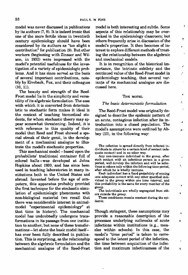
ful to introduce anotherparameter here, in orderto clarify the definition ofthis probability of effec-tive contact. If there areM individuals in the en-tire population, thenp(M - 1) = K = the ex-pected number of con-tacts experienced by eachindividual during onetime period.)

We argue that, during time period t, theprobability that a susceptible individualcomes in contact with none of the cases isqCi. The complement of this term describesthe probability that a susceptible individ-ual contacts at least one case, and hencecontracts the infection.

0 1 2 3 4 9 6 7 8 9 1 0 I I

TIME PERIOD (t)

FIGURE 1. Epidemic course predicted by the basic Reed-Frost model, assuming So = 100, Co = 1 andp =0.02. The successive numbers of cases (solid line) and numbers of remaining susceptibles (dotted line) wereobtained by iteration of equations 2 and 3 in the text. The expected numbers of cases were rounded off totheir nearest integer values. Given these conditions, a total epidemic size of 79 cases is predicted by.thedeterministic Reed-Frost model, and 22 susceptibles remain still unaffected at its conclusion.

90 PAUL E. M. FINE

Probability a susceptible contacts atleast one case during time period t

= (1 - qc'). (1)

The expected number of cases in the nexttime interval is thus defined deterministi-cally as:

And, of course:

St + l = St-Ct + 1 (3)

These two equations comprise the basicReed-Frost model. Iteration of these equa-tions for successive time periods allows theprediction of an entire epidemic, as illus-trated in figure 1.

The implications of this formulationhave been investigated by a number ofauthors. Notable are Wilson and Burke's(9) comparison of the model with the ear-lier "mass action" formulations of Hamer(13) and Soper (14), Costa Maia's (15) in-vestigation of the implications of addingnew susceptibles, and Zinsser and Wilson's(4) examination of the effect of variationsin virulence upon the apparent case fatal-ity rates in such theoretical epidemics.

The stochastic formulation

The conversion from deterministic tostochastic formulation is easily illustratedby comparing a Reed-Frost epidemic proc-ess to a series of binomial trials. In eachtime period, each ofthe S, susceptible indi-viduals "has" a probability of becominginfected equal to (1 - qCl). We can thusimagine the events of one time period to beanalogous to the tossing of S/ "coins," eachof which has a probability of (1 - qCl) offalling "cases up." And the probabilitythat exactly r of the susceptibles ("coins")become infected (fall "cases up") is thusgiven by the standard binomial expres-sion:

Prob (Ct + , = r)

'« ~ r)\(4)

This is the basic stochastic formulation ofthe Reed-Frost epidemic process. Theequation defines the probability of a speci-fied prevalence (Ct + t = r) in the subse-quent time period, given some set of initialconditions (St,Ct andp). By multiplicationof probabilities denned by this equation, itis possible to calculate the probability thatany specified series of prevalences wouldoccur (e.g., C,+ ,, Ct + 2, C, +"3, . . .), givensome initial conditions. Abbey (12) dis-cussed this formulation, and from it de-rived a maximum likelihood method forestimating the p value for any given epi-demic sequence.

Though the derivation of the stochasticexpression 4 is straightforward, and acces-sible to anyone familiar with the binomialdistribution, its implications may not be soimmediately clear. This reflects a commondifficulty suffered by non-mathematicianswhen dealing with stochastic equations.Although stochastic epidemics may easilybe generated on a computer, in accordancewith this equation, the conceptual leapfrom expression 4 to print-out is sometimesunderestimated by biostatisticians whopresent such material to non-mathemati-cal audiences. It is here that the mechani-cal analogue to the Reed-Frost model dem-onstrates its usefulness as a teaching tool.

The mechanical model

The goal is (or was) to design a simplemechanical apparatus which would illus-trate the behavior of the stochastic Reed-Frost epidemic. Indeed, the absence ofelectronic computers when the model wasfirst developed made some such apparatusnecessary for the empirical exploration—let alone teaching—of the model. The tech-nique developed at the Johns HopkinsUniversity (Sartwell (8) attributes theidea to Reed) involved the use of coloredballs to represent the individuals in thepopulation, and their randomized lineararrangement in a trough to illustrate theoutcome of each successive time period

THE REED-FROST EPIDEMIC MODEL 91

TOP VIEW

SJDC VIEW

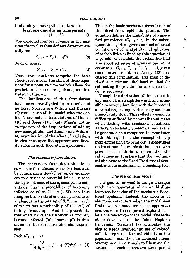
FIOUEB 2. Two different types of mechanical Reed-Frost models. 2a is the classic trough, holding a lineararrangement of "susceptible," "case," "immune" and "contact neutralizer" balls. Convenient teachingmodels may include one fixed and one removable endpiece, to facilitate pouring balls back into a containerfor randomizing. Sloping the trough makes it easier to achieve a linear arrangement 2b is a roulette-wheeltype model, this one containing 50 equal-sized pockets in its circumference. A phonograph turntable may beused to rotate such a wheel. Balls are spun into the wheel independently, and all those which land in thesame pocket are said to have "effective contact"

(figure 2A). The simplest convention wasdescribed by Elveback and Varma (16) asfollows.

Balls of four different colors are re-quired; "susceptibles" (e.g., S = green);"cases" (e.g., C = red); "immune" (e.g.,/ =blue) and "blocks," or "contact neutraliz-ers" (e.g., N = white). Numbers of ballsrepresenting the individuals of each sta-tus, during one time period, are placed in acontainer along with a number of blocks(the determination of their number is dis-cussed below). These are randomized, andpoured into a trough in single file. It isthen considered that all individuals (col-ored balls) which are not separated by ablock have contact during that period—thus any "susceptible ball" which is notseparated by at least one block from a"case ball" is considered to experience in-fectious contact. The sequence is consid-ered to be closed-ended, in that no contactoccurs between balls at opposite ends ofthe file. After the result (i.e., the incidenceof new cases) has been recorded, the popu-lation of balls is then altered accordingly:"case balls" being substituted for suscepti-bles which experienced infectious contact;

TABLE 1

Interpretation of a linear sequence of balls m thestandard Reed-Frost trough model. The conventionassumes that a case remains infectious for one time

period and then becomes permanently immune.Substitutions are made prior to randomization ofballs for simulation of the subsequent time period

Random sequencefor time period t

Substitutions requiredfor simulation of

subsequent time period(t + 1)

BlockSusceptibleImmuneCaseBlockCaseSusceptibleSusceptibleBlockSusceptibleBlock

Case

Immune

ImmuneCase

-*• Case

and "immune balls" being substituted forcases (see table 1). The entire procedure isthen repeated . . . , until the epidemic ex-pires due to absence of cases or exhaustionof susceptibles. The results of three such

92 PAUL E. M. FINE

20

m is

4 3 « 7

TIME PERIOD (t)

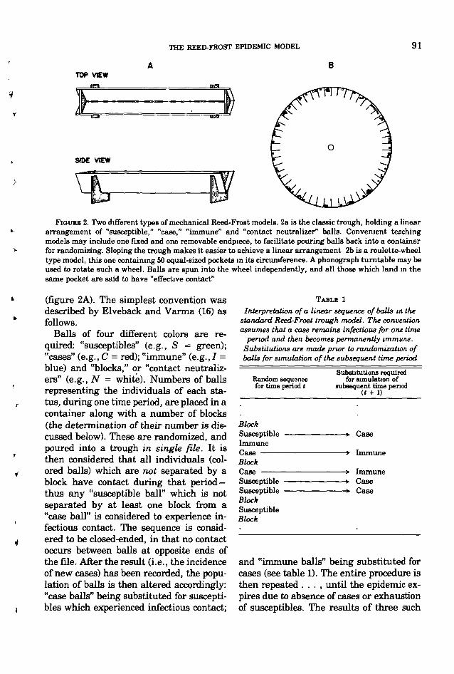
FIOUBB 3. Resuita of three separate epidemic simulations with a Reed-Frost trough model. Eachsimulation began with 100 initial susceptibles and a single index case. 98 "block" balls were maintainedthroughout the process. The total numbers of cases to evolve in the three epidemics were- 1 ( ),73 ( ) and 84 ( ).

epidemic simulations are presented in fig-ure 3.

Such an exercise provides a vivid dem-onstration of the role of chance in a simpleepidemic process. Of course, the conven-tions may be changed in numerous ways-for example: new susceptibles may be in-troduced into the population at any rate;some susceptibles can be converted di-rectly to immune status, to mimic an im-munization program; and the duration ofinfectiousness or immunity may be variedat will.

This is apparently the sort of model orig-inally developed at Johns Hopkins about1930, and is the one which has been widelyused in teaching since that time. It may benoted that any technique for obtaining arandom linear ordering of S, C, I and Nunits may be substituted for the tradi-tional ball and trough apparatus. An ob-vious alternative would be to use cards in

place of the balls, which can then be ran-domized by shuffling. This may have beenthe technique used by Horiuchi and Sugi-yama (17, 18), who described their tech-nique as "using similar chips and manyshufflings." It remains for us to discuss therelationship between such mechanicalmodels and the algebraic formulation 4.

Relationship between the mechanical andmathematical models

The initial problem is to relate the con-tact probabilities as defined in the mathe-matical formulation (expressions 1 and 4)to the probabilities of contact between sim-ulated individuals in the mechanical Reed-Frost model.

The probability of contact p was definedas the probability that any two individualschosen at random from the populationwould have contact during one time pe-riod. This can easily be expressed in terms

THE REED-FROST EPIDEMIC MODEL 93

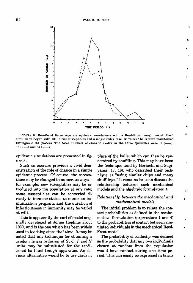
of the linear mechanical model, by investi-gating the probability that two specifiedcolored-ball individuals, X and Y, will notbe separated by a block. Assuming thatthere are n blocks, then, no matter whereX should fall, there will be two positionsout of a total of (n + 2) for Y to have"effective contact" with X. This is illus-trated in figure 4. Therefore, 2/(n +2) de-fines p, the probability that any two indi-viduals come in contact in a random se-quence, and [1 - 2/(n + 2)] = n/(n + 2)gives the probability that two individualswill not be in contact in a sequence, or q.

It would be convenient if this simplerelationship were sufficient to equate themechanical and the mathematical forms ofthe Reed-Frost model. But it is not. A diffi-culty arises in that the crucial term in thestochastic expression 4 is not the proba-bility that a susceptible individual con-tacts a single case, but the probability thata susceptible individual will contact atleast one case during the time period.(This is a crucial difference, as it distin-guishes the Reed-Frost model from theearlier mass-action models of Hamer (13)and Soper (14)). In the algebraic formula-tion this probability could be expressed as(1 - qCl); but it turns out that it cannot beexpressed in terms of blanks merely bysubstituting n/(n + 2) for q. This is so

because of a peculiar linear dependence insuch a random sequence of balls.

The difficulty does not arise if there isonly a single infectious case in the trough"population"; as under this circumstancethe probability of contact with one case isequivalent to the probability of contactwith at least one case, and equals p, or 2/(n + 2). But, let us assume that there weremore than a single case, say Ct = 2. If wealso assume that there were two blockballs, then n = 2, andp = 2/(2 + 2) = 0.5.On the basis of this value of p, the proba-bility that a susceptible contacts at leastone of the cases should be, according toexpression 1, equal to 1 - (1 - 0.5)2 = 0.75.But this does not apply to a linear arrange-ment of balls, say two blocks, two cases,and one susceptible. A few moments withpencil and paper, exploring the possiblepermutations and combinations of fivesuch objects, will suffice to convince thereader that the probability the "suscepti-ble ball" contacts at least one "case ball,"under the linear arrangement convention,is not 0.75, but 0.7. This is illustrated intable 2.

Rather than depend only upon penciland paper permuting, a general equationfor the contact probabilities in the me-chanical model can easily be derived (Ap-pendix A). We find that the probability a

SAMPLEBALL SEQUENCE-

SPACE NUMBERS

SUCCESSFULCONTACT POSITIONS'

T" T" T" T" T" T"

T" T"

n.2

FIOUHE 4. Contact probabilities between two colored balls, balls X and Y, in a linear arrangement of n"block" balls: balls 1,2, • • -n. Given n "blocks" and ball X, in any linear sequence, there are (n + 2) possible(and equally probable) positions for ball Y. Only two of these (e.g., positions 4 and 5 in the illustratedsequence) involve contact with ball X. The probability of contact between the two colored balls, in the linearmodel, is therefore 2/(n + 2).

94 PAUL E. M FINE

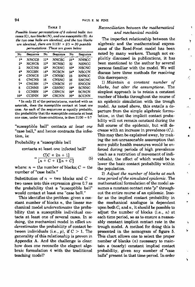
TABLE 2

Possible linear permutations of 5 colored balls: twocases (C), two blocks (N), and one susceptible (S).Asthe two case balls are identical, and the two blocksare identical, there are 511(2! x 21) = 30 possible

permutations. These are given below

No

1*2*34*5*67*89

10*

Sequence

NNCCSNCNCSNCCNSNCCSNCNNCSCNCNSCNCSNCCNNSCCNSNCCSNN

No.

11*12*13*14*15*1617*18*19*20*

Sequence

NNCSCNCNSCNCSNCNCSCNCNNSCCNSNCCNSCNCSNNCCSNCNCSCNN

No

21*2223*24*25262728*29*30*

Sequence

NNSCCNSNCCNSCNCNSCCNSNNCCSNCNCSNCCNSCNNCSCNCNSCCNN

* In only 21 of the permutations, marked with anasterisk, does the susceptible contact at least onecase. As each of the sequences is equally probable,the probability that the susceptible contacts at leastone case, under these conditions, is then 21/30 = 0.7

"susceptible ball" contacts at least one"case ball," and hence contracts the infec-tion, is:Probability a "susceptible ball

contacts at least one infected ball"C[C + 2n + 1]

[n + C + l][n + C] ( '

where: n = the number of blocks; C = thenumber of "case balls."

Substitution of n = two blocks and C =two cases into this expression gives 0.7 asthe probability that a "susceptible ball"would contact at least one "case ball."

This identifies the problem: given a con-stant number of blocks n, the linear me-chanical model underestimates the proba-bility that a susceptible individual con-tacts at least one of several cases. In sodoing, the mechanical model in effect un-derestimates the probability of contact be-tween individuals (i.e., p), if C > 1. Thegenerality of this relationship is proven inAppendix A. And the challenge is cleanhow does one reconcile the elegant alge-braic formulation 4 with the traditionalteaching model?

Reconciliation between the mathematicaland mechanical models

The imperfect relationship between thealgebraic and the mathematical expres-sions of the Reed-Frost model has beennoted by many workers. Though not ex-plicitly discussed in publications, it hasbeen mentioned to the author by severalpersons familiar with the model. We willdiscuss here three methods for resolvingthis discrepancy.

1) Maintain a constant number ofblocks, but alter the assumptions. Thesimplest approach is to retain a constantnumber of blocks throughout the course ofan epidemic simulation with the troughmodel. As noted above, this entails a de-parture from the simple algebraic formu-lation, in that the implicit contact proba-bility will not remain constant during thefull course of the epidemic, but will de-crease with an increase in prevalence (C<).This may then be explained away, by mak-ing the not-unreasonable assumption thatsome public health measures would be en-forced during periods of high prevalence(such as a restriction of movement of indi-viduals), the effect of which would be tolower the basic contact probability withinthe population.

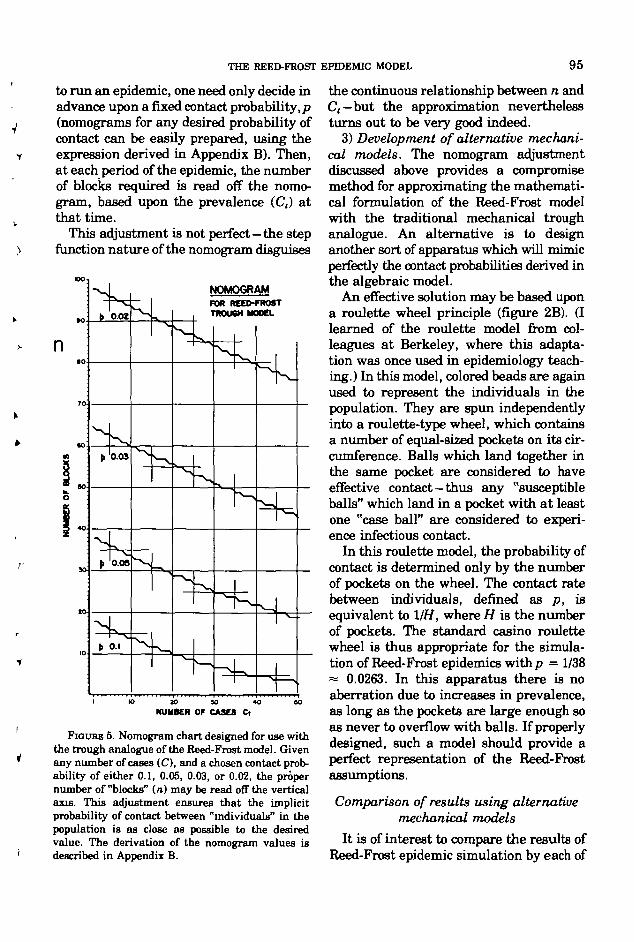
2) Adjust the number of blocks at eachtime period of the simulated epidemic. Themathematical formulation of the model as-sumes a constant contact rate "p" through-out the entire course of an epidemic. Inso-far as the implied contact probability inthe mechanical analogue is dependentupon both Ct and n, it should be possible toadjust the number of blocks (i.e., n) ateach time period, so as to ensure a reason-ably constant implicit contact rate in thetrough model. A method for doing this ispresented in the nomogram of figure 5.This chart allows one to select the propernumber of blanks (n) necessary to main-tain a (nearly) constant implied contactprobability, given any number of "caseballs" present in that time period. In order

4

4

THE REED-FROST EPIDEMIC MODEL 95

to run an epidemic, one need only decide inadvance upon a fixed contact probability, p(nomograms for any desired probability ofcontact can be easily prepared, using theexpression derived in Appendix B). Then,at each period of the epidemic, the numberof blocks required is read off the nomo-gram, based upon the prevalence (C,) atthat time.

This adjustment is not perfect—the stepfunction nature of the nomogram disguises

NOMOGRAMFDR REED-FROSTTROUGH MOOD.

10 20 30 40 90

NUMBER OF CASES Ct

FIGURE 5. Nomogram chart designed for use withthe trough analogue of the Reed-Frost model. Givenany number of cases (C), and a chosen contact prob-ability of either 0.1, 0.05, 0.03, or 0.02, the propernumber of "blocks" (n) may be read off the verticalaxis. This adjustment ensures that the implicitprobability of contact between "individuals" in thepopulation is as close as possible to the desiredvalue. The derivation of the nomogram values isdescribed in Appendix B.

the continuous relationship between n andC(—but the approximation neverthelessturns out to be very good indeed.

3) Development of alternative mechani-cal models. The nomogram adjustmentdiscussed above provides a compromisemethod for approximating the mathemati-cal formulation of the Reed-Frost modelwith the traditional mechanical troughanalogue. An alternative is to designanother sort of apparatus which will mimicperfectly the contact probabilities derived inthe algebraic model.

An effective solution may be based upona roulette wheel principle (figure 2B). (Ilearned of the roulette model from col-leagues at Berkeley, where this adapta-tion was once used in epidemiology teach-ing.) In this model, colored beads are againused to represent the individuals in thepopulation. They are spun independentlyinto a roulette-type wheel, which containsa number of equal-sized pockets on its cir-cumference. Balls which land together inthe same pocket are considered to haveeffective contact—thus any "susceptibleballs" which land in a pocket with at leastone "case ball" are considered to experi-ence infectious contact.

In this roulette model, the probability ofcontact is determined only by the numberof pockets on the wheel. The contact ratebetween individuals, defined as p, isequivalent to 1IH, where H is the numberof pockets. The standard casino roulettewheel is thus appropriate for the simula-tion of Reed-Frost epidemics withp = 1/38= 0.0263. In this apparatus there is noaberration due to increases in prevalence,as long as the pockets are large enough soas never to overflow with balls. If properlydesigned, such a model should provide aperfect representation of the Reed-Frostassumptions.

Comparison of results using alternativemechanical models

It is of interest to compare the results ofReed-Frost epidemic simulation by each of

§0.

ID

10

L10

MODEL I

CONSTANT NUMBER OF BLOCKS (0=98)

MEAN: 62.812

MEDIAN- 77

90TOTAL CASES PER EPIDEMIC

100

iLJOQ.IdU.

o

e

90

10

I

MODEL 2

NOMOGRAM ADJUSTMENT Of (n)

MEAN 64.956

MEDIAN^ 80

4

4

10 90TOTAL CASES PER EPIDEMIC

100

5°Ul9Q.UJU.OITUlOD

I 10

MODEL 3

EXACT p = 0.O2

MEAN: 65.12

MEDIAN: 80

10 . 90TOTAL CASES PER EPIDEMIC

100

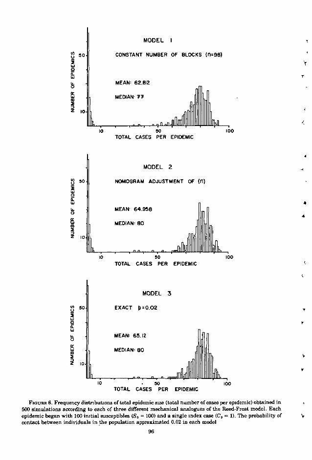
FIOURB 6. Frequency distributions of total epidemic size (total number of cases per epidemic) obtained in500 simulations according to each of three different mechanical analogues of the Reed-Frost model. Eachepidemic began with 100 initial susceptibles (So = 100) and a single index case (Co = 1). The probability ofcontact between individuals in the population approximated 0.02 in each model

96

THE REED-FROST EPIDEMIC MODEL 97

these three mechanical model analogues.Ironically enough, such a comparison ismost easily made using electronic com-puter simulation; as this avoids any biaseswhich might be introduced by the con-struction and operation of the several me-chanical models. Appropriate contactprobabilities for each of the three mechani-cal models can be defined in mathematicalterms, and used as the basis for computersimulations.

The results presented here were derivedby the simulation of Reed-Frost epidemicswith So = 100, Co = 1, andp = 0.02. Theappropriate probability of infection for asusceptible (i.e., the probability a suscep-tible contacts at least one case) was calcu-lated at each generation, based upon thenumber of cases present. For model 1, theprobability of infection was adjusted ac-cording to expression 5, maintaining aconstant n = number of blocks = 98. Formodel 2, the probability of infection wasdetermined by a two-step process. First thenumber of blocks (n) was adjusted accord-ing to the nomogram (i.e., as the nearestinteger solution to expression 14 in Appen-dix B, with p = 0.02). The probability ofinfection was then calculated by insertingthis n into expression 5. For model 3, theprobability of infection was obtained onthe basis of equation 1, with q = 0.98 (= 1

- P ) .The experience of each susceptible indi-

vidual was then determined by compari-son with a separate random number (uni-formly distributed between 0 and 1); andthe entire process was then repeated foreach time period, until termination of theepidemic. The results are illustrated infigure 6, in terms of the frequency distri-bution of total epidemic size, based upon500 separate epidemics generated by eachof the three methods.

Not surprisingly, the mean and medianepidemic sizes using model 1 are slightlysmaller than with either of the othermodels. This is to be expected, as its condi-tions entail a lowering of effective contactrate during periods when the prevalence

exceeds a single case. On the other hand,it is interesting to note how closely theresults of models 2 and 3 concur. This indi-cates the effectiveness of the nomogramadjustment technique in maintaining thecontact rate at a constant level.

CONCLUSIONS

The mechanical model developed byReed and Frost is one of the major land-marks in the history of theoretical epide-miology. Its development coincided withthe introduction of stochastic methodologyin the late 1920s; and it probably providedthe first technique for generating empiri-cal solutions to a probabilistic epidemicmodel. But its importance for us today isfar more than merely historical. Thoughelectronic computers may have replacedsuch colored-ball models in empirical re-search on stochastic processes, the dra-matic illustration of the play of chancewhich is afforded by such models makesthem as useful today as in the past. In onesense, the model's usefulness today isgreater than ever, in that it now mayserve as an effective introduction to thelarge body of stochastic epidemic theorywhich has accumulated in recent years.

The publication history of the Reed-Frost model is remarkable for its delays.Just as there was a lag of many yearsbefore the basic algebraic formulation ofthe model was first published, so there hasbeen an even longer delay in discussion ofthe properties of its mechanical analogue.Many of those who have used the modelhave undoubtedly noted the theoreticalproblems discussed in this commentary;and a variety of different solutions maywell have been developed. Though thosewho have made such developments may,like Reed and Frost, have considered themas "too slight a contribution" for publica-tion, it is hoped that others will profit fromthis discussion of the model's properties;and that this may encourage further de-velopment and use of this highly instruc-tive and ingenious form of epidemic mod-elling.

98 PAUL E M. FINE

REFERENCES

1. Bailey NTJ: The Mathematical Theory of Infec-tious Diseases and Its Applications. London,Charles Griffin and Co, 1975

2. Ross R: Report on the Prevention of Malaria inMauritius. London, Waterlow, 1908

3. Fine PEM: Ross's o priori pathometry — a per-spective. Proc R Soc Med 68:547-551, 1975

4. Zinsser H, Wilson EB: Bacterial dissociationand a theory of the rise and decline of epidemicwaves. J Prev Med 6:497-514, 1932

5. Muench H: Catalytic Models in Epidemiology.Cambridge, Harvard University Press, 1959

6. Macdonald G: The Epidemiology and Control ofMalaria. London, Oxford University Press, 1957

7. Frost WH: Some conceptions of epidemics ingeneral. Am J Epidemiol 103:141-151, 1976

8. Sartwell PE: Memoir on the Reed-Frost epi-demic theory. Am J Epidemiol 103:138-140,1976

9. Wilson EB, Burke MH. The epidemic curve.Proc Natl Acad Sci USA 28:361-367, 1942

10. Elveback LR, Fox JP, Ackerman E, et al: Aninfluenza simulation model for immunizationstudies. Am J Epidemiol 103:152-165, 1976

11. Fox JP, Elveback L, Scott W, et al: Herd immu-nity: basic concept and relevance to publichealth immunization practices. Am J Epidemiol94:179-189, 1971

12. Abbey H: An examination of the Reed Frosttheory of epidemics. Hum Biol 24:201-233, 1952

13. Hamer WH: Epidemic disease in England. Lan-cet 1:733-739, 1906

14. Soper HE: Interpretation of periodicity in dis-ease-prevalance. J Roy Statist Soc 92:34-73,1927

15. Costa Maia JDO: Some mathematical develop-ments on the epidemic theory formulated byReed and Frost. Hum Biol 24:167-200, 1952

16. Elveback L, Varma A: Simulation of mathemat-ical models for public health problems. PublicHealth Rep 80:1067-1076, 1965

17. Horiuchi K, Sugiyama H: A criticism of theReed-Frost theory from the standpoint of sto-chastic epidemiology. Jap J Public Health2(suppl):355, 1955 (in Japanese)

18. Horiuchi K, Sugiyama H: On the importance ofMonte Carlo approach in the research of epide-miology. Osaka City Med J 4:59-62, 1957

APPENDIX A

Consider a linear sequence of balls in atrough. We assume there are C "caseballs" and n "blocks," and calculate theprobability that there will be at least oneblock between the specified susceptibleand any "case ball."

Examine the sequence with no caseballs, that is, containing only the n blocksand the specified "susceptible ball." By the

argument illustrated in figure 4, we seethat there are n out of (n + 2) chances for asingle "case ball" to miss contact with thesusceptible. If we assume that the first"case ball" does in fact fail to contact thesusceptible, then, by a similar argument,the probability that a second case also failsto contact the susceptible is given by (n +1)1 (n + 3). And the probability that a thirdcase also misses contact with the suscepti-ble would be (n + 2)/(/i + 4). This argu-ment is repeated for each of the C "caseballs" present. And the probability that allof the C "case balls" escape contact withthe susceptible is the product of all theseprobabilities, or

n (n + 1)(n + 2) (n +

(» +(n +

which reduces

3)

2)4) '

to:

n(n H

(«H

( * J

HI)

h C -hC +

1)1)

(h + C + 1) (n + C)'

(6)

(7)

We are more interested in the complementof this probability, or the probability thatat least one of the "case balls" does contactthe specified susceptible. This is obtainedby subtraction:

1 -n(n + 1)

[n + QC(C + 2n + 1)

(n + C + l)(n + C) '(8)

This is expression 5 in the text. It shouldbe noted that the presence of immunes, orof other susceptibles, has no bearing onthis derivation; as their position in thesequence will have no effect on whether ornot the specified "susceptible ball" con-tacts at least one "case ball." This is sobecause of the convention that all coloredballs which are not separated by a blockhave effective contact. Contact occurs"through" susceptibles or immunes, butnot through the blocks. For this reason itmakes no difference whether "recovered"

THE REED-FROST EPIDEMIC MODEL 99

case balls are removed from the simula-tion, or are changed to immune balls—theresultant epidemic curve should not be af-fected.

Expression 7, which describes the proba-bility that a "susceptible ball" contacts nocases, is analogous to the expression qCl in •the mathematical formulation of the Reed-Frost model. By equating the two expres-sions, we can derive a general descriptionof the "q" value which is implicit in thetrough analogue. And this must be thecomplement of the probability of contactCp") between individuals which is implicitin the trough model convention:

(l -n(n + 1)

(n + C + l)(n + C) (9)

or

n(n + 1){n + C + l)(n + O. (10)

where "p" refers to the implicit probabilityof contact between any two individuals inthe population, as apparent in the troughmodel.

According to the basic assumptions ofthe Reed-Frost model, the value of "p"should remain constant throughout thecourse of an epidemic. On the other hand,expression 10 suggests that its apparentvalue in the trough model will be depend-ent upon the prevalence, i.e., upon thenumber of "case balls" (C). Indeed, we candemonstrate that if n remains constant asthe number of "case balls" in the troughincreases, the implicit "p" value will infact decrease. We compare:

n{n Yc

with

P c + i

_ I= 1 ~ \

{n + C

n(n

YC)J

(n + C+

To show that "p"c > " p " a i , w e need toprove that

nin +1]V/C>i(n (n + C)J

n(n{(n + C + 2)(n + C + 1))

By subtracting one from both sides, multi-plying through by minus one, and raisingboth sides to the power C, we have

+ l)(n + C)r n(ra +

< L(» + C + 2)(«2)(n + CSince

C+ 1= 1 - C+ 1'

the right hand side can then be factorized,and inverted, and the preceding inequalitymay be rewrittenn + C + 2

n + C

[{n + C + 2)(n + C + 1)

n{n+ 1 )i i/<c + i)

— '

or

h + C + 2 l C + 1

L « + c J(ra + C + 2)(n + C + 1)n(n • ( }

We then prove expression 12 by inductiononC.

Expression 12 is clearly true for C = 1,by substitution:

[n + 3]* (n + 3)(n + 2)U + 1J n(n + 1) '

as this is equivalent to:n(n + 3) < (n + l)(n + 2),

which is true for all n.Assuming expression 12, we must show

that it remains valid when C is replaced by

100 PAUL E M. FINE

C + 1, namely

u + c + IJ3)(n + C + 2)

n(ra + 1)

Recognizing that

n + C + 3 n + C + 2/i + C + 1 n + C

Vn + C + 31 c + i rn + C + 21 c + i[n + C + lj < [ n + C J

we use expression 12 to write the inequal-ity:

[n + C + 1

{n + C + 2)(ra + C + 1)< n(n + 1)

Now multiply both sides by (n + C + 3)/(n+ C + 1), to get expression 13, which com-pletes the proof.

APPENDIX B

We wish to adjust the number of blocksin the mechanical model so that the proba-

bility a "susceptible ball" contacts at leastone "case ball" is commensurate with aconstant probability of contact between in-dividuals in the population. We thus wishto maintain the "implicit p" value, as de-fined in Appendix A, constant throughouta simulation exercise. This may be done bysolving equation 9 for n, in terms of/? andC. A quadratic is obtained:

2C(1 -

(1 - "p")c - 1= 0 (14)

For any values of 0 < "p" < 1 and C > 0,the constant term in this equation must benegative, and thus there can be but a sin-gle positive root n. These positive roots areplotted in the nomogram of figure 4. Theroots have been rounded off to their near-est integer values, in order to facilitate useof the nomogram with the mechanicalReed-Frost model.

In order to prepare a nomogram for anydesired contact probability, one need onlysubstitute that value into expression 14and solve it repeatedly with successive in-teger values for C.