Alternative Thinking - AQR Capital Management · PDF file · 2016-12-15Alternative Thinking ... climb up the efficient frontier toward more-concentrated positions in the riskier asset

AQR Capital Management, LLC

Two Greenwich Plaza

Greenwich, CT 06830

p: +1.203.742.3600

f: +1.203.742.3100

w:aqr.com

Thinking

Strategic Portfolio Construction: How to Put It All Together

This issue discusses strategic portfolio construction,

focusing on top-down decisions where mean-

variance optimization, always to be used carefully, is

of even more limited use. How to combine

traditional asset classes with illiquids or with

alternative risk premia? How much illiquidity,

leverage and shorting to allow? The answers — and

thus major portfolio choices — are largely driven by

investor beliefs and constraints.

Alternative

Second Quarter

2015

Alternative Thinking | Strategic Portfolio Construction: How to Put It All Together 1

Executive Summary

Portfolio construction is challenging even when

combining comparable investments such as

stocks and bonds. When mixing traditional and

alternative assets, the challenges are multiplied.

Mean-variance optimization is a useful tool for

portfolio construction but it has many pitfalls.

Its use is particularly limited when we make top-

down portfolio decisions on characteristics

beyond the mean-variance framework. For

example, how much leverage and shorting to

allow, or how much to allocate to illiquid

investments, when an optimizer often keeps

saying “more”? How should we weigh across

diversifiers of traditional portfolios: alternative

risk premia versus illiquid assets or versus

manager-specific alpha?

Such top-down decisions are largely driven by

investor-specific beliefs and constraints. We

describe portfolios both based on formal

optimizations and on such subjective judgments.

Introduction

Portfolio construction is such a broad topic that it

requires a book to cover the subject thoroughly.1

Here we only cover some big themes on strategic

asset allocation decisions (ignoring liabilities).

Mean-variance optimization (MVO) is the classic

portfolio construction workhorse, and its key

insights are a natural starting point. One way to

summarize unconstrained MVO is that as a baseline

it allocates equal volatility to different investments

but then it tilts toward investments with higher

Sharpe ratios and/or lower correlations.

MVO works best when the allocation problem

involves a small number of comparable investable

assets, and the assumptions underlying MVO are

broadly satisfied. Even then, estimation errors in

1 Some excellent books already exist; see Successful Investing Is a Process by Lussier (2013) and Portfolio Construction and Risk Budgeting by Scherer (2015). These topics are also covered in Active Portfolio Management by Grinold and Kahn (1999), Asset Management by Ang (2014) and Introduction to Risk Parity and Budgeting by Roncalli (2014).

inputs — especially expected returns — are a serious

problem, and unconstrained MVO can suggest

extreme positions. The Appendix discusses MVO’s

uses and pitfalls in more detail.

MVO is less useful when we combine traditional and

alternative investments. We show the MVO results

for allocating between traditional asset classes,

illiquid “endowment alternatives” (defined below),

and liquid alternative risk premia, given plausible

inputs. Not surprisingly, unconstrained optimizers

love illiquidity, leverage and shorting in a portfolio.

Investors often respond to unreasonable results by

adding constraints: ruling out leverage and shorting

or setting even narrower ranges for acceptable

weights. Indeed, when top-down decisions involve

portfolio characteristics beyond the MVO

framework, real-world choices are largely driven by

investor-specific beliefs and constraints.2 We finish

with some practical portfolio proposals based on

such inherently subjective considerations and only

loosely guided by optimization results.

MVO and Top-Down Portfolio Decisions

Some of the most important top-down decisions in

portfolio construction depend on investor tolerance

for portfolio volatility, leverage, illiquidity and short-

selling (as well as views on how well these features

are rewarded by markets). Only the first, the

mean/volatility tradeoff, is naturally captured in the

MVO framework. Examples below show that, under

common investor assumptions, MVO tends to load

up on leverage, illiquidity and shorting unless these

are explicitly constrained or penalized. While it is

possible to impose such constraints, MVO does not

help in deciding how tight the constraints should be.

We present MVO results for several universes,

starting from the simple stocks (EQ) vs. bonds (FI)

case, then broaden to include illiquid “endowment

alternatives” (EALTS, such as private equity, hedge

funds, real estate) and later also liquid alternative

2 In geek-speak they end up at corner solutions where your basic beliefs and constraints are fully driving the outcome and the optimizer is not adding any value.

2 Alternative Thinking | Strategic Portfolio Construction: How to Put It All Together

risk premia (ARP, such as a diversified portfolio of

long/short style premia or hedge fund risk premia).3

We contrast the results of long-only, leverage-

constrained optimizations (capital weights must be

non-negative and sum to 100%) and unconstrained

versions, as well as the impact of two different

volatility targets.

The results, of course, reflect the inputs we give. Our

expected return, volatility and correlation estimates

are shown in Exhibit 1. We use forward-looking

estimates, partly guided by long-run historical

experience, but erring to the conservative side versus

history with one exception: We use a deliberately

optimistic assumption for the Sharpe ratio of

EALTS so as to make our case for ARP rest mainly

on diversification (as opposed to Sharpe ratio).4 We

welcome readers to challenge these assumptions.

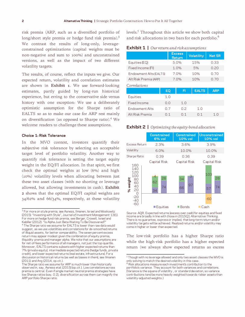
Choice 1: Risk Tolerance

In the MVO context, investors quantify their

subjective risk tolerance by selecting an acceptable

target level of portfolio volatility. Another way to

quantify risk tolerance is setting the target equity

weight in the EQ/FI allocation. In that spirit, we first

check the optimal weights at low (6%) and high

(10%) volatility levels when allocating between just

these two asset classes (with no shorting or leverage

allowed, but allowing investments in cash). Exhibit

2 shows that the optimal EQ/FI capital weights are

34/62% and 66/34%, respectively, at these volatility

3 For more on style premia, see Asness, Ilmanen, Israel and Moskowitz (2015): “Investing with Style”, Journal of Investment Management 13(1). For more on hedge fund risk premia, see Berger, Crowell, Israel and Kabiller (2012): “Is Alpha Just Beta Waiting To Be Discovered?” 4 The Sharpe ratio we assume for EALTS is lower than raw data would suggest, as we use volatilities and correlations for de-smoothed returns of illiquid assets, for better comparability. The seven percent excess return may appear modest given the combination of equity premia, illiquidity premia and manager alpha. We note that our assumptions are for net-of-fees performance of all managers, not just the top-quartile. Moreover, EALTS contains subsets with higher expected returns than 7% (private equity), intermediate expected returns (hedge funds, private credit), and lower expected returns (real estate, infrastructure). For a discussion on historical returns (as well as biases in them), see Ilmanen (2011) and Ang (2014, op.cit.). The Sharpe ratio we assume for ARP is much lower than historically observed in, say, Asness etal. (2015) (op.cit.). Low correlations across premia is central. Even if single market-neutral premia strategies have low Sharpe ratios (say, 0.2), diversification across them can magnify the ARP portfolio Sharpe ratio.

levels.5 Throughout this article we show both capital

and risk allocations in two bars for each portfolio.6

Exhibit 1 | Our return and risk assumptions

Excess

Return Volatility Net SR

Equities (EQ) 5.0% 15% 0.33

Fixed Income (FI) 1.0% 5% 0.20

Endowment Alts (EALTS) 7.0% 10% 0.70

Alt Risk Premia (ARP) 7.0% 10% 0.70

Correlations

EQ FI EALTS ARP

Equities 1.0

Fixed Income 0.0 1.0

Endowment Alts 0.7 0.2 1.0

Alt Risk Premia 0.1 0.1 0.1 1.0

Exhibit 2 | Optimizing the equity-bond allocation

Constrained 6% vol

Constrained 10% vol

Unconstrained 10% vol

Excess Return 2.3% 3.6% 3.9%

Volatility 6.0% 10.0% 10.0%

Sharpe Ratio 0.39 0.36 0.39

Source: AQR. Expected returns (excess over cash) for equities and fixed income are broadly in line with those in 2015Q1 Alternative Thinking. There is no guarantee, express or implied, that long-term return and/or volatility targets will be achieved. Realized returns and/or volatility may come in higher or lower than expected.

The low-risk portfolio has a higher Sharpe ratio

while the high-risk portfolio has a higher expected

return (we always show expected returns as excess

5 Though with no leverage allowed and only two asset classes the MVO is only solving to match the desired volatility in this case. 6 Risk allocations measure each investment’s contribution to the portfolio’s variance. They account for both variances and correlations. (Variance is the square of volatility , or standard deviation, so variance contributions tend be more heavily weighted towards riskier assets than volatility-adjusted weights.)

34 74 66

97 57 74

62 26 34

3 103

26 4

-60

-60-40-20

020406080

100120140160

Capital Risk Capital Risk Capital Risk

% w

eig

ht

Equities Bonds Cash


over cash). However, if we allow leverage (third

column), the optimal portfolio is the tangency

portfolio (see Box) levered up to the required

volatility level — this offers somewhat higher

expected returns than the leverage-constrained

version at the higher volatility target.

Choice 2: Leverage vs. Concentration

Exhibits 2 and 3 are also helpful for discussing the

second major top-down choice — between leverage

and concentration. Many investors are leverage

averse or constrained. To achieve higher risk and

return targets they do not lever up the tangency

portfolio but, instead, climb up the efficient frontier

toward more-concentrated positions in the riskier

asset class.7 That is, in our figure they travel up the

purple not the green line (see Exhibit 3 in the Box).

These investors forfeit the higher risk-adjusted

returns available on the capital market line in favor

of raw returns. Investors with lower risk and return

targets may be able to benefit from optimal

diversification without needing to face this tradeoff

between leverage and concentration. Since investors

are presumably willing to own cash (with leverage

being the willingness to “short” cash) they can move

along the green not purple lines as long as they are

staying to the left of the tangency point.

For most investors, leverage constraints lead to

portfolios that are not well diversified by risk. This

has a negative impact on expected returns (in the

case of Exhibit 2, the difference between the

leverage-constrained and -unconstrained portfolios

is 0.3%), and this gap increases at higher levels of

volatility. Assuming cost-effective access to leverage,

a portfolio on the capital market line will be

expected to outperform a portfolio on the efficient

frontier. Empirical evidence over long periods has

tended to support this theory.8

7 In a two-asset case, the efficient frontier contains just varying mixes of EQ and FI. In multi-asset cases, this frontier contains the highest-return portfolios at each vol level. Adding more risky assets to the investment universe tends to move the frontier northwest (higher Sharpe ratios). 8 See, for example, Asness, Frazzini and Pedersen (2012): “Leverage Aversion and Risk Parity,” Financial Analysts Journal 68(1).

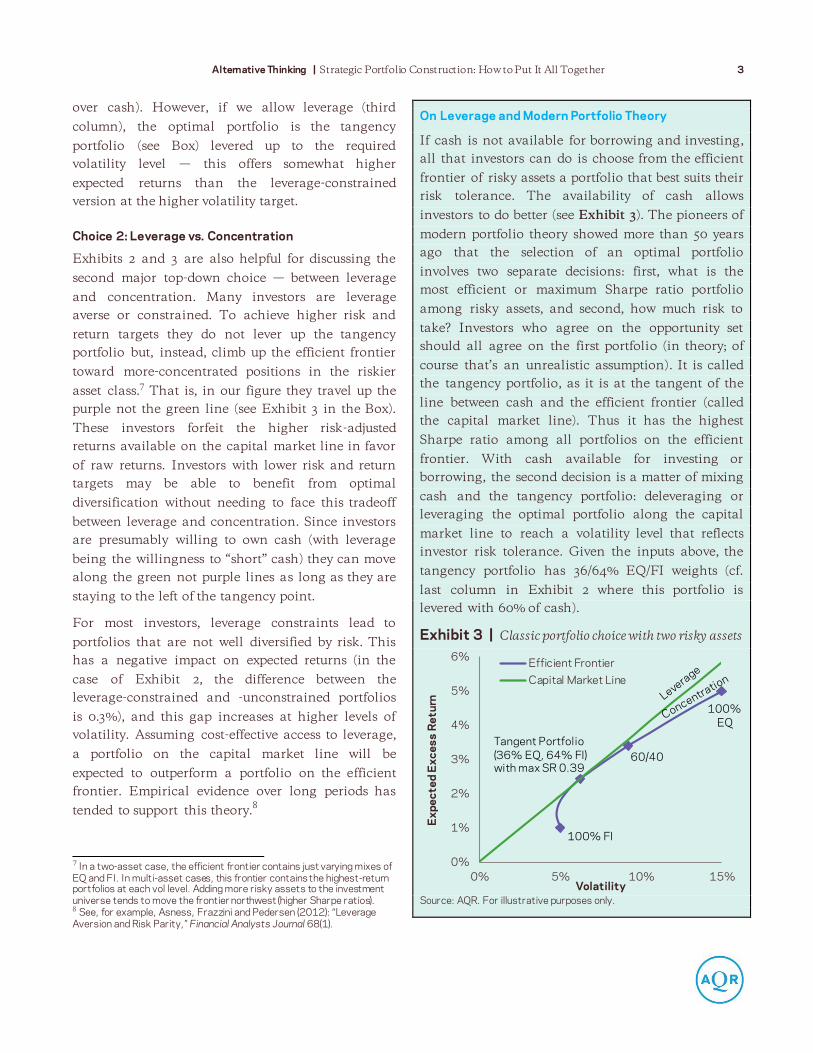
On Leverage and Modern Portfolio Theory

If cash is not available for borrowing and investing,

all that investors can do is choose from the efficient

frontier of risky assets a portfolio that best suits their

risk tolerance. The availability of cash allows

investors to do better (see Exhibit 3). The pioneers of

modern portfolio theory showed more than 50 years

ago that the selection of an optimal portfolio

involves two separate decisions: first, what is the

most efficient or maximum Sharpe ratio portfolio

among risky assets, and second, how much risk to

take? Investors who agree on the opportunity set

should all agree on the first portfolio (in theory; of

course that’s an unrealistic assumption). It is called

the tangency portfolio, as it is at the tangent of the

line between cash and the efficient frontier (called

the capital market line). Thus it has the highest

Sharpe ratio among all portfolios on the efficient

frontier. With cash available for investing or

borrowing, the second decision is a matter of mixing

cash and the tangency portfolio: deleveraging or

leveraging the optimal portfolio along the capital

market line to reach a volatility level that reflects

investor risk tolerance. Given the inputs above, the

tangency portfolio has 36/64% EQ/FI weights (cf.

last column in Exhibit 2 where this portfolio is

levered with 60% of cash).

Exhibit 3 | Classic portfolio choice with two risky assets

Source: AQR. For illustrative purposes only.

0%

1%

2%

3%

4%

5%

6%

0% 5% 10% 15%

Ex

pe

cte

d E

xc

es

s R

etu

rn

Volatility

Efficient Frontier

Capital Market Line

100% FI

100%

EQ

Tangent Portfolio

(36% EQ, 64% FI) with max SR 0.39

60/40


It may seem puzzling that so many institutions

choose risk concentration but there are clear reasons

for it. In fact, the average investor must do it

because a global wealth portfolio of all assets

displays concentrated equity risk. Despite this,

financial markets have not rewarded equities with a

uniquely high Sharpe ratio, likely due to prevalent

leverage aversion.9 Less-constrained investors may

be able to diversify better and enhance returns at the

expense of the constrained majority.

Choice 3: Liquid vs. Illiquid

Another important top-down choice relates to

illiquid investments. It would be possible to harvest

illiquidity premia within equity and bond markets

by overweighting less-liquid securities, but here we

represent illiquidity with “endowment alternatives”

(EALTS) due to their popularity among

endowments. The best-known proponent, the Yale

Endowment, allocates more than 75% of its portfolio

to alternative assets such as private equity, hedge

funds and real estate. Harvesting illiquidity premia

is only a part of the motivation; another is that well-

selected (“first-quartile”) managers can better add

alpha in less-competitive private markets.10

We assume that a well-diversified combination of

EALTS can offer 7% excess returns (even after fees)

at 10% volatility, for an admirable Sharpe ratio of

0.7. However, in line with historical experience of

less-impressive diversification benefits, we assume

an equity market correlation of 0.7 (see Exhibit 1).

If one simply looks at historical data on EALTS they

would show too low estimate of volatility and

correlations. This is because these returns are

9 Leverage aversion is so common because many investors recall infamous episodes caused by excessive leverage. While leverage can help investors diversify better, it undoubtedly carries a risk that must be carefully managed. One key precept is to avoid mixing leverage and illiquidity, a combination responsible for several past portfolio blowups. 10 Not all investors can select those first-quartile managers, and illiquidity premia may not be as high as often expected — if investors overpay for the artificial smoothness in illiquid-asset returns. We expect to tackle some of these topics in future research. We do think that the illiquidity premium is one important source of long-run returns, among many. It especially suits investors with a long horizon and limited liquidity needs, and who use little leverage, shorting, dynamic rebalancing or risk targeting (these do not mesh well with illiquids).

artificially smoothed as the assets are not regularly

(by choice or impossibility) marked-to-market. Our

volatility and correlation assumptions are meant to

be our guess of the real values if they were not

artificially smoothed.11

Optimizers would be even

more impressed with the smooth raw series and

would make even larger allocations in EALTS than

below if we used such inputs.

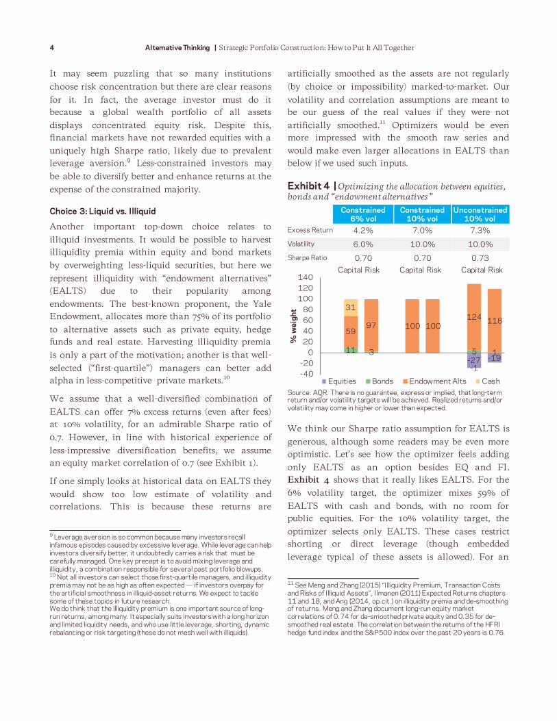
Exhibit 4 | Optimizing the allocation between equities,

bonds and “endowment alternatives”

Constrained 6% vol

Constrained 10% vol



Volatility 6.0% 10.0% 10.0%


Source: AQR. There is no guarantee, express or implied, that long-term return and/or volatility targets will be achieved. Realized returns and/or volatility may come in higher or lower than expected.

We think our Sharpe ratio assumption for EALTS is

generous, although some readers may be even more

optimistic. Let’s see how the optimizer feels adding

only EALTS as an option besides EQ and FI.

Exhibit 4 shows that it really likes EALTS. For the

6% volatility target, the optimizer mixes 59% of

EALTS with cash and bonds, with no room for

public equities. For the 10% volatility target, the

optimizer selects only EALTS. These cases restrict

shorting or direct leverage (though embedded

leverage typical of these assets is allowed). For an

11 See Meng and Zhang (2015) “Illiquidity Premium, Transaction Costs and Risks of Illiquid Assets”, Ilmanen (2011) Expected Returns chapters 11 and 18, and Ang (2014, op.cit.) on illiquidity premia and de-smoothing of returns. Meng and Zhang document long-run equity market correlations of 0.74 for de-smoothed private equity and 0.35 for de-smoothed real estate. The correlation between the returns of the HFRI hedge fund index and the S&P500 index over the past 20 years is 0.76.

-27 -19 11 3 5 1

59 97 100 100

124 118

31

-1 -40

-20

0

20

40

60

80

100

120

140Capital Risk Capital Risk Capital Risk

% w

eig

ht

Equities Bonds Endowment Alts Cash


unconstrained 10% volatility target, the optimizer

does not demand much leverage but does increase

the EALTS position to 124% by shorting public

equities. While this is not realistic for most, or

recommended (shorting equities to lever up illiquid

assets is about as scary as it sounds), it is also not

surprising; this is indeed typical of MVO. When an

optimizer sees two assets with dissimilar Sharpe

ratios and a high correlation, it wants to create a

long/short position to exploit this opportunity —

investing more in EALTS but hedging part of equity-

directional risk by shorting the inferior asset.

Choice 4: Long-Only vs. Long/Short

If MVO prefers an asset with a higher Sharpe ratio

than traditional assets despite a high correlation

with them, how would it treat an investment which

combines a high Sharpe ratio with low correlations?

Yes, we’d expect love at first sight.

Here we add alternative risk premia (ARP) to the

investment universe alongside the existing triplet.

We assume similar expected return and volatility

and the same 0.7 Sharpe ratio as for EALTS, but

thanks to shorting it is possible to create market-

neutral positions that have only 0.1 correlation with

major asset class returns. 12

(ARP can actually target

zero correlation but we assume a mild positive

number here.) To us, a highly diversified composite

of long/short premia has the most credible shot at

achieving a sustainably high Sharpe ratio. One

challenge is that when ARP’s high Sharpe ratio

reflects diversification and thus volatility reduction,

it will require meaningful leverage to achieve the

10% volatility target (we assume 8x: 4x longs and 4x

shorts — though we assume some of these strategies

involve bonds which explains much of the required

leverage; without bonds assumed Sharpes would be

somewhat lower and leverage much lower).

The main message from Exhibit 5 is that in

reasonable situations, MVO prefers the better-

diversifier ARP over EALTS, though both have a

12 Here we refer to shorting within ARP. The optimizations in Exhibits 2-5 will allow or not allow shorting of the asset classes as described.

useful role. But it is worth going through some

counterintuitive results where ARP are not favored,

as these illustrate complications with MVO.

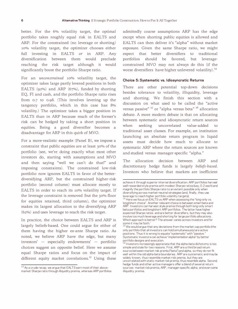
Exhibit 5 | Optimizing the allocation between equities,

bonds, endowment alts and alt risk premia

Panel A: Unconstrained equity allocation

Constrained 6% vol

Constrained 10% vol



Volatility 6.0% 10.0% 10.0%


Panel B: Minimum 30% equity allocation

Constrained

6% vol Constrained

10% vol Unconstrained

10% vol


Volatility 6.0% 10.0% 10.0%


Source: AQR. There is no guarantee, express or implied, that long-term return and/or volatility targets will be achieved. Realized returns and/or volatility may come in higher or lower than expected.

Again, equities are trumped and get assigned zero or

negative weights, and bonds do not fare much

-24 -13 1

-9 -1

40 50

100 100 92 66

40 50

67

48 18

-25 -60

-40

-20

0

20

40

60

80

100

120

140


% w

eig

ht

Equities BondsEndowment Alts Alt Risk PremiaCash

30

62

30 40 30 33

14

2

15 2 2

2 62 58

31

22

33

34 8 2

62

44 21

-39

-40

-20

0

20

40

60

80

100

120


% w

eig

hts

Equities BondsEndowment Alts Alt Risk PremiaCash

OR 100% ARP

(dead heat)


better. For the 6% volatility target, the optimal

portfolio takes roughly equal risk in EALTS and

ARP. For the constrained (no leverage or shorting)

10% volatility target, the optimizer chooses either

full investing in EALTS or in ARP. Any

diversification between them would preclude

reaching the risk target although it would

significantly boost the portfolio Sharpe ratio.

For an unconstrained 10% volatility target, the

optimizer takes large partly levered positions in both

EALTS (92%) and ARP (67%), funded by shorting

EQ, FI and cash, and the portfolio Sharpe ratio rises

from 0.7 to 0.98. (This involves levering up the

tangency portfolio, which in this case has 8%

volatility.) The optimizer takes a bigger position in

EALTS than in ARP because much of the former’s

risk can be hedged by taking a short position in

equities. Being a good diversifier becomes a

disadvantage for ARP in this quirk of MVO.

For a more-realistic example (Panel B), we impose a

constraint that public equities are at least 30% of the

portfolio (see, we’re doing exactly what most other

investors do, starting with assumptions and MVO

and then saying “well we can’t do that!” and

imposing constraints). The constrained low-risk

portfolio now ignores EALTS in favor of the better-

diversifying ARP, but the constrained higher-risk

portfolio (second column) must allocate mostly to

EALTS in order to reach its 10% volatility target. If

the leverage constraint is removed (but the 30% floor

for equities retained, third column), the optimizer

makes its largest allocation to the diversifying ARP

(62%) and uses leverage to reach the risk target.

In practice, the choice between EALTS and ARP is

largely beliefs-based. One could argue for either of

them having the higher ex-ante Sharpe ratio. As

noted, we believe ARP have the edge, but many

investors’ — especially endowments’ — portfolio

choices suggest an opposite belief. Here we assume

equal Sharpe ratios and focus on the impact of

different equity market correlations.13

Using these

13 As a crude recap, we argue that EALTS earn most of their above-market Sharpe ratio through illiquidity premia, whereas ARP portfolios

admittedly coarse assumptions ARP has the edge

except when shorting public equities is allowed and

EALTS can then deliver it’s “alpha” without market

exposure. Given the same Sharpe ratio, we might

expect that better diversifiers to traditional

portfolios should be favored, but leverage-

constrained MVO may not always do this (if the

worse diversifiers have higher unlevered volatility).14

Choice 5: Systematic vs. Idiosyncratic Returns

There are other potential top-down decisions

besides tolerance to volatility, illiquidity, leverage

and shorting. We finish this section with a

discussion on what used to be called the “active

versus passive” 15

or “alpha versus beta” 16

allocation

debate. A more modern debate is that on allocating

between systematic and idiosyncratic return sources

when seeking uncorrelated value-added to

traditional asset classes. For example, an institution

launching an absolute return program in liquid

assets must decide how much to allocate to

systematic ARP where the return sources are known

and studied versus manager-specific “alpha.”

The allocation decision between ARP and

discretionary hedge funds is largely beliefs-based.

Investors who believe that markets are inefficient

achieve it through superior internal diversification. ARP portfolios harvest well-rewarded style premia with modest Sharpe ratios (say, 0.2 each) and magnify the portfolio Sharpe ratio to an extent possible only when diversifying across market-neutral strategies (and, finally, they use leverage to reach higher portfolio volatility targets). 14 Here we focus on EALTS vs ARP when assessing the “long-only vs. long/short choice”. Another relevant choice is between smart beta and ARP. Investors can harvest style premia through both long-only smart beta portfolios and long/short ARP portfolios. The latter have higher expected Sharpe ratios and are better diversifiers, but they may also involve too much leverage and shorting for large portfolio allocations. Which approach is better? The answer varies across investors and for some it may be ‘both.’ 15 We would argue that any deviations from the market cap portfolio (the only portfolio that all investors can hold simultaneously) are active positions. Thus it is wrong to equate “systematic” with ”passive.” Systematic investors can achieve “implementation alpha” by better portfolio designs and execution. 16 Investors increasingly appreciate that the alpha-beta dichotomy is too simple and stale for two reasons. First, ARP are a third broad return source between market risk premia (“beta”) and alpha, so they do not fit well within the old alpha-beta boundaries. ARP are systematic and may be widely known, thus resemble market-risk premia, but they are uncorrelated with static market risk premia, thus resemble alpha. Second, hedge funds and other active managers offer a blend of several return sources: market risk premia, ARP, manager-specific alpha, and even some illiquidity premia.


and that they can identify in advance superior

managers who can exploit these inefficiencies are

more likely to make large hedge fund allocations.

Investors who believe more in cost-effective

harvesting of diverse systematic return sources tend

to favor ARP.17

These two avenues need not be

mutually exclusive, and the optimal allocation may

well be a mixture. While we can debate the relative

Sharpe ratios, empirically it does seem clear that

hedge fund portfolios have much higher equity

market correlations than ARP portfolios do

(suggesting the allocation decision is similar to that

between EALTS and ARP above).

Problems With MVO

We have already seen hints of problems with MVO.

MVO is most useful when its underlying

assumptions are broadly satisfied (e.g., if investors

care only about portfolio means and variances) and

when we have reasonable inputs for the optimizer.

The Appendix discusses the two related problems

for the MVO: model errors and estimation errors.

When it comes to top-down portfolio allocation

decisions, constraints are particularly important.

We saw above that even with reasonable inputs,

unconstrained MVO can give results that are

unacceptable to most real-world investors: zero or

negative allocations to traditional asset classes and

heavy exposure to illiquidity, leverage and shorting.

No wonder then that constraints against these

features dominate actual portfolios.

We made a closely related observation in Alternative

Thinking 2013Q1 when we showed that an

unconstrained MVO, with reasonable inputs, would

allocate 23% of its risk to long-only market risk

premia and 77% to long/short ARP. In reality, most

17 Belief in market efficiency is not a key distinction: both hedge funds and ARP harvest various risk-based return premia and market inefficiencies. It is also ironic that the putatively idiosyncratic hedge fund “alphas” are in practice more correlated with market risk premia than are systematic ARP (since the latter are designed to be market-neutral). For single hedge funds, idiosyncratic alpha may be as large as beta, but it diversifies away in a broad multi-manager portfolio, leaving a much bigger role for systematic exposures. This feature explains how single hedge funds may have equity correlation of, say, 0.3-0.4, on average, while a broad hedge fund portfolio may have 0.7 equity correlation.

investors allocate most risk to the former. We argued

that four “Cs” — conviction (beliefs), constraints

(against leverage and shorting), conventionality and

capacity — drive real-world portfolio choices.

How can investors then select reasonable

constraints? Sometimes laws, regulations or

liabilities force the constraints on them. More often,

constraints are self-imposed, perhaps guided by peer

behavior, which creates a self-perpetuating

convention or gradual herding among institutions.18

We think a better approach is for investors to

consider carefully their key beliefs and preferences,

and then make judgmental choices that combine the

broad spirit of optimization — diversify widely but

tilt toward higher risk-adjusted returns and

diversifiers — with investor-specific priors and

constraints. Optimization results above give helpful

direction to the allocations, but rarely the final

result.

Putting It Together — Practical Examples

In this last section, we show some concrete

examples of how we let our beliefs — and

preferences and constraints — guide our top-down

decisions on portfolio allocations, and how other

institutions might make different choices. The

portfolios below are not optimized but heuristic, due

to the subjective nature of beliefs and constraints.

Exhibit 6 shows several portfolio allocations and the

portfolio statistics based on our inputs listed below.

(As before, these are forward-looking assumptions,

guided by historical experience.) All these portfolios

are consistent with our core beliefs in that they

involve more aggressive diversification than

traditional portfolios (and use leverage and shorting

to get there). But they all differ in some respect from

one another; investors can judge from portfolio

characteristics as well as from performance and risk

statistics which one fits them best.

18 What is deemed conventional among institutional investors does evolve over time, albeit slowly. Examples include rising equity allocations since the 1960s and the growing role of alternatives in 2000s.


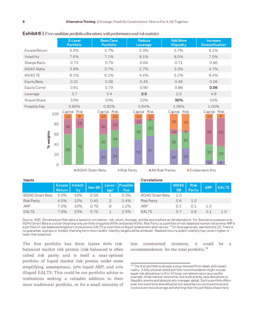
The first portfolio has three layers: 60% risk-

balanced market risk premia (risk-balanced is often

called risk parity and is itself a near-optimal

portfolio of liquid market risk premia under some

simplifying assumptions), 30% liquid ARP, and 10%

illiquid EALTS. This could be our portfolio advice to

institutions seeking a valuable addition to their

more traditional portfolio, or for a small minority of

less constrained investors, it could be a

recommendation for the total portfolio.19

19 The first portfolio is already a step removed from ideals and toward reality. A fully unconstrained portfolio recommendation might include equal risk allocations to 8 to 10 lowly correlated return sources (for example, three market risk premia, five style premia, plus allocations to illiquidity premia and idiosyncratic manager alpha). Such a portfolio offers even more extreme diversification but would be too unconventional and involve even more leverage and shorting than the portfolios shown here.

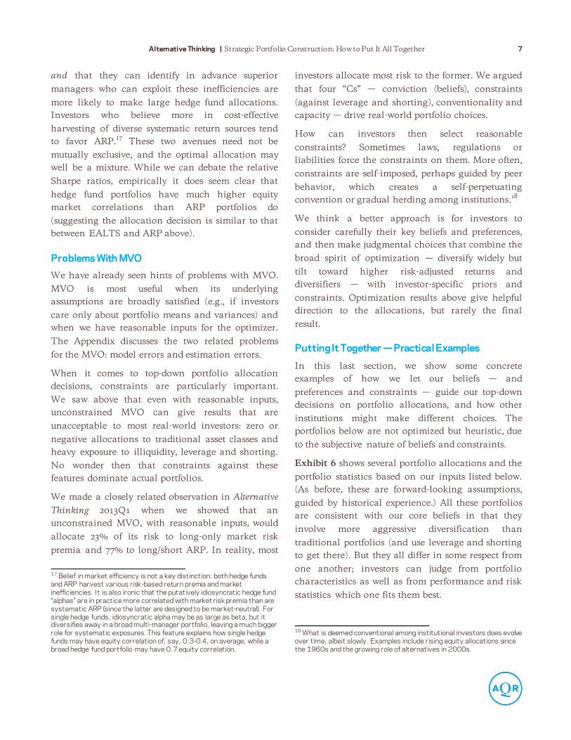
Exhibit 6 | Five candidate portfolio allocations, with performance and risk statistics

3-Layer

Portfolio

Base Case

Portfolio

Reduce

Leverage

Add More

Illiquidity

Increase

Diversification

Excess Return 5.5% 5.7% 5.3% 5.7% 6.1%

Volatility 7.6% 7.1% 8.1% 8.0% 7.0%

Sharpe Ratio 0.73 0.79 0.64 0.71 0.86

60/40 Alpha 3.9% 3.7% 2.7% 3.3% 4.7%

60/40 TE 8.1% 6.1% 4.4% 5.2% 8.4%

Equity Beta 0.31 0.38 0.49 0.46 0.26

Equity Correl 0.61 0.79 0.90 0.86 0.56

Leverage 3.7 3.4 2.0 2.0 4.8

Illiquid Share 10% 10% 10% 30% 10%

Possible Fee 0.85% 0.82% 0.64% 1.08% 1.00%

Source: AQR. Simulated portfolio data is based on correlation, risk, return, leverage, and fee assumptions as detailed above. For illustrative purposes only. 60/40 Smart Beta is a style-tilted long-only portfolio of equities (60% and bonds (40%). Risk Parity is a portfolio of risk-balanced market risk premia. ARP is a portfolio of risk-balanced long/short style premia. EALTS is a portfolio of illiquid “endowment alternatives.” * On leverage levels, see footnote 20. There is no guarantee, express or implied, that long-term return and/or volatility targets will be achieved. Realized returns and/or volatility may come in higher or lower than expected.

30 34 50

57

30 33

10 8

60 72

30 34

30 30

30 31

30 28

30 19

30 22

10 3

10 3 50 55

10 9 10 10 10 10

30 33

10 8

0

20

40

60

80

100Capital Risk Capital Risk Capital Risk Capital Risk Capital Risk

% w

eig

hts

60/40 Smart Beta Risk Parity Alt Risk Premia Endowment Alts

Inputs Correlations

Excess

Return

Volatil-

ityNet SR

Lever-

age*

Possible

Fee

60/40

SB

Risk

ParityARP EALTS

60/40 Smart Beta 5.0% 10% 0.50 1 0.3% 60/40 Smart Beta 1.0

Risk Parity 4.5% 10% 0.45 2 0.4% Risk Parity 0.6 1.0

ARP 7.0% 10% 0.70 8 1.2% ARP 0.1 0.1 1.0

EALTS 7.0% 10% 0.70 1 2.5% EALTS 0.7 0.6 0.1 1.0


The first portfolio has attractive expected return

characteristics (5.5% over cash, Sharpe ratio 0.73),

but is still too unconventional for most institutions’

total portfolio (under our assumptions its tracking

error vs. 60/40 is 8% and employs look-through, i.e.,

counting the leverage in the risk parity and ARP

strategies themselves, leverage of 3.7)20

.

The second portfolio is our base case. We split the

market risk premia component, investing half of the

60% allocation in a long-only 60/40 stock/bond

portfolio with style tilts (denoted by “smart beta.”

even if we are not fans of this term)21

and retaining

half in risk parity. This change makes the portfolio

more realistic for a total portfolio solution, as the

tracking error to 60/40 is now 6% and leverage

somewhat reduced. Expected return is actually

mildly higher (5.7%) and volatility lower, resulting in

a higher Sharpe ratio (0.79). However, this portfolio

is a worse diversifier to traditional 60/40 portfolios

(offering slightly lower alpha and a much higher

equity correlation).22

Note that this base-case portfolio harvests style

premia through both the long-only 60/40 portfolio

and the long/short ARP portfolio. Investors who

want large style exposures may find that their

20 Leverage is a topic that would require a longer treatment. Many investments ranging from public and private equities to hedge funds contain embedded leverage, but we follow here the common practice of quoting their leverage as 1. In contrast, we quote the leverage of risk parity and ARP (2 and 8, respectively) at higher standards, given their better transparency. The look-through leverage is the gross sum of all the long and short positions divided by assets under management (or the fund NAV). Using the same treatment as we use for hedge funds, we could instead quote these as investments with leverage 1 since for end-investors these are unlevered investments into levered vehicles (which, moreover, contain plentiful free cash). 21 Smart beta portfolios are long-only portfolios tilted toward one well-rewarded style such as value (and less often toward multiple styles). We believe that a multi-style approach is superior and that an efficient multi-style-tilted 60/40 stock/bond portfolio can achieve about 5% excess return over cash and 0.5 net Sharpe ratio (if we assume 3.5% and 0.35 for the “passive” cap-weighted 60/40 portfolio). These assumptions are conservative compared to the historical evidence on the excess returns of style-tilted equity and bond portfolios; see, for example, Frazzini, Israel, Moskowitz and Novy-Marx (2013) “A New Core Equity Paradigm” and Israel and Richardson (2015) “Investing with Style in Corporate Bonds.” 22 Being more conventional (having a lower tracking error versus traditional portfolios) and being a worse diversifier (having a higher equity market correlation) are really two sides of the same coin. There is an inherent tradeoff between these two goals. Whether an investor cares more about conventionality or about absolute diversification benefits tells whether it is more peer oriented or total return oriented. Over the long run, we believe the latter approach will give better portfolio performance.

constraints against leverage and shorting limit their

allocations to ARP portfolios, and they may want to

add style exposures further through smart beta.

We now analyze three tweaks to the base case

portfolio and assess the impact of each on expected

performance and risk characteristics.23

Reduce leverage: Compared to the base case, we

shift 20% from levered long/short style premia

(ARP) to unlevered long-only style-tilted portfolios

(60/40 Smart Beta). This switch actually gives us the

most conventional portfolio (lowest tracking error

vs. 60/40 of 4.4%, highest equity correlation of 0.90),

and the look-through leverage falls to 2. This option

likely has the biggest capacity as well. Of course,

there is a cost: the Sharpe ratio drops from 0.79 to

0.64, while expected return drops from 5.7% to 5.3%.

Add more illiquidity: Compared to the base case, we

again shift 20% from ARP, this time to illiquid

EALTS. Because we do not penalize EALTS for

embedded leverage, this variant too shows portfolio

leverage at 2. Compared to the previous switch, this

one shows a smaller decline in the Sharpe ratio (to

0.71) and a smaller increase in equity correlation (to

0.86). Fees are meaningfully higher.

Increase diversification: Compared to the base case,

we do the opposite shift to that in “reduce leverage,”

now increasing ARP by 20% at the expense of the

long-only style-tilted allocation. Not surprisingly,

better diversification results in the highest Sharpe

ratio (0.86), lowest volatility and lowest equity

correlation (0.56) but also the highest leverage and

tracking error versus 60/40. This portfolio would be

the most consistent with our core beliefs, but also

the least conventional. The previous three portfolio

options may be more palatable for most investors.

23 We actually tried one more tweak, lowering costs, but will just summarize the key results here. Compared to the base case, using cap-weighted 60/40 instead of smart beta 60/40 would lower typical portfolio fees by 0.08% but would also cut net expected return by 0.5% and Sharpe ratio by 0.06. Given our input assumptions, style tilts are worth doing.


Concluding Thoughts

Many investors ask for our thoughts on “putting it

all together.” This article does not give definitive

answers, or even recommend a particular framework

for making such decisions. Instead, we start from

our quantitative home territory (inputs such as

expected returns, volatilities and correlations) and

then explore how investor-specific beliefs and

constraints can inform and interact with formal

optimization methods. We will continue to study

this topic as part of a two-way discussion with

investors, in an effort to help them build portfolios

that best meet their own particular investment

objectives, constraints and beliefs.


Appendix: MVO — Its Uses, Pitfalls and Remedies

MVO works well with many portfolio problems

Although MVO is an effective tool for portfolio

construction, many investors eschew using it, partly

because of problems described below. Others would

stick with MVO and try to deal with these problems

by some modifications. We take a middle path in the

main text when describing MVO results but then

arguing that certain top-down decisions are so

complex that they may be better done heuristically,

only guided by the insights from optimizations.

Yet, to be clear, we find optimizers very useful in

many portfolio problems, and they are central to

both our research and portfolio construction

process. We cannot go deep into these topics here,

but we offer one illustration of a portfolio problem

where MVO gives helpful insights and reasonable

portolio weights. Here we allocate risk across four

style premia: value, momentum, carry, defensive.

The optimizer maximizes the portfolio Sharpe ratio

while requiring that weights amount to 100%.

We assume that each of the four strategies targets

15% annual volatility. In the baseline case, we

assume all the strategies have equal long-term

expected Sharpe ratios of 0.4 (thus 6% expected

return over cash), and that all the strategy pairs

are uncorrelated. Not surprisingly, an optimizer

would give equal risk allocations to all the

strategies. With four uncorrelated return sources,

expected portfolio volatility would be 7.5% and

the portfolio Sharpe ratio would double to 0.8.

If we change the inputs so that one style pair, let’s

say value and momentum, have an appealing

negative correlation of -0.5, the optimizer assigns

twice as large risk weight (33% vs. 17%) to these

better complements than to the other two style

premia. The improved diversification reduces

portfolio volatility further and boosts the Sharpe

ratio to 0.98.

We can also ask what Sharpe ratio we’d have to

assume for value and momentum if all styles

were uncorrelated, to give the same risk weights

as the negative correlation did (33% vs. 17%). The

answer is 0.57, so the -0.5 value-momentum

correlation is as valuable as a 0.17 rise in the

Sharpe ratio of these two premia (both

assumptions give an equal boost to the optimal

portfolio’s Sharpe ratio).

This is just one example where an optimizer

provides insights about the worth of good

diversifiers, apart from its core task: mapping inputs

into actionable outputs (portfolio weights). The

optimizer gave reasonable solutions partly because

the inputs were reasonable and the portfolio

constituents were comparable in the MVO

framework, so we didn’t need to impose constraints.

Problems with MVO … and some remedies

MVO uses information on means, volatilities and

correlations. The general optimality condition for

the unconstrained case is that in the maximum

Sharpe ratio portfolio the ratio of marginal

contribution of return to marginal contribution of

risk is the same for all assets. This condition ensures

that we cannot improve the portfolio by marginal

reallocations between constituent assets.

MVO is most useful when (i) its underlying

assumptions are broadly satisfied (investors care

only about portfolio means and variances or these

two moments capture well the investment

opportunity set — this requires near-normal return

distributions and liquid investments) and (ii) we

have reasonable inputs for the optimizer. We

address next the two corresponding classes of

problems for the MVO: (i) model errors and (ii)

estimation errors.

Model errors: Clearly, investors care about portfolio

characteristics beyond mean and variance. We have

highlighted above liquidity, leverage and shorting

aversions; other preferences may include higher

moments (e.g., skewness) or ethical considerations.

The biggest error may be that we are dealing with

the wrong question. Perhaps a broader question is

needed than the typical optimization across

financial asset holdings. A corporate pension plan

may broaden its perspective from asset

optimization, include pension liabilities and

optimize the asset-liability surplus, or the corporate


sponsor may go further and try to optimize even

broader enterprise risk. Likewise, the optimization

problem of a retirement saver may be broadened to

include human capital and the housing wealth.24

Estimation errors: Even for the simple MVO

question we need to use reasonable inputs for

expected returns, volatilities and correlations.

Estimation error is the difference between the

estimated value and the true value of a parameter.

Expected returns are especially susceptible to

estimation errors (returns are harder to predict than

volatilities and correlations) and the optimizer

output (portfolio weights) is especially sensitive to

expected return inputs. Recall in Exhibit 5 the

optimizer’s reaction to seeing two strongly positively

correlated assets with different Sharpe ratios: it

seeked to create a large long/short position between

EALTS and EQ to exploit this apparent opportunity.

Unconstrained optimizers (not just MVO) can often

create extreme positions, concentrated risk and high

turnover due to estimation errors.

Thus, care is needed when choosing the inputs.25

Using historical volatilities and correlations may be

reasonable in many cases, but plain use of historical

average returns without any adjustment is a recipe

for trouble. Shrinking estimates toward some

reasonable priors (such as zero or group average)

often helps. It may make sense to give bigger weight

to the inputs you trust than those you don’t.

In practice, estimates of means are the least reliable,

or the most susceptible to estimation errors. Thus,

several popular portfolio construction approaches

avoid using the expected return information.

Implicitly, these often assume that risk-adjusted

24 Potential model errors don’t stop there. Investment returns are hardly normally distributed (though downside risk measures may be nearly proportional to volatility). Multiple risk sources, time-varying expected returns, multiperiod hedging needs, capacity concerns and market frictions are other challenges hard to fit to the MVO framework. 25 The choice of investable assets also matters. Investments with problematic characteristics (illiquid assets; options and other assets with highly asymmetric distributions; investments with limited histories or prone to structural changes) should be avoided in typical MVOs. Ideally, there are a reasonable number of distinct investable blocks with high intra-group correlations and low inter-group correlations. A large number of assets creates problems unless factor structure is used to drastically reduce the number of estimated parameters in a covariance matrix.

returns are similar across assets (or that the

estimates are highly uncertain).26

Full MVO would

be superior if expected return or risk-adjusted return

differences between assets were so large that we

could reliably estimate them.

Instead of giving up on expected return information,

one could try to make the optimization better

behaved. As noted, shrinking inputs may help.

Another possibility is to use robust optimization, a

formal technique that directly considers the

uncertainty in data (estimation errors).

In many practical portfolio construction problems,

AQR uses a modified optimization approach to

make the outputs reasonable, while anchoring them

to our unconstrained views and risk models. We first

generate a theoretical portfolio based on our

predictive models that we would hold in the absence

of constraints or transaction costs; we use this

portfolio’s weights and an input covariance matrix

to reverse-engineer our unconstrained implied

expected returns. In the second step we put these

implied expected returns together with our

covariance matrix as well as constraints and

transaction cost estimates into a robust optimizer

that comes up with the final optimal weights.

Even if we can tame estimation errors, model errors

remain a problem for top-down portfolio decisions

which are not neatly captured by just mean and

variance. Extending MVO to capture some missing

element (say, illiquidity, leverage aversion or higher

moments) results in a more complex model where

more parameters need to be estimated, increasing

the potential for estimation errors. And in practice,

we cannot deal with all these dimensions in one

model, so constraints must be imposed.

26 The simplest portfolio construction approach is equal weighting (1/N). The next simplest, equal volatility weighting, uses only volatility as an input, while equal risk contribution (full risk parity) uses both volatility and correlation inputs. The latter two weighting schemes coincide with the maximum Sharpe ratio portfolio (full MVO result) if all assets have equal Sharpe ratios and zero or equal correlations. Two other weighting schemes, the minimum variance and maximum diversification portfolios, also use volatility and correlation inputs. Their optimality condition is different, however, resulting in larger weights for low-risk assets.


Disclosures

This document has been provided to you solely for information purposes and does not constitute an offer or solicitation of an offer or any advice or

recommendation to purchase any securities or other financial instruments and may not be construed as such. The factual information set forth herein has

been obtained or derived from sources believed by the author and AQR Capital Management, LLC (“AQR”) to be reliable but it is not necessarily all-

inclusive and is not guaranteed as to its accuracy and is not to be regarded as a representation or warranty, express or implied, as to the information’s

accuracy or completeness, nor should the attached information serve as the basis of any investment decision. This document is intended exclusively for

the use of the person to whom it has been delivered by AQR, and it is not to be reproduced or redistributed to any other person. The information set forth

herein has been provided to you as secondary information and should not be the primary source for any investment or allocation decision. This document

is subject to further review and revision.

Past performance is not a guarantee of future performance

This presentation is not research and should not be treated as research. This presentation does not represent valuation judgm ents with respect to any

financial instrument, issuer, security or sector that may be described or referenced herein and does not represent a formal or official view of AQR.

The views expressed reflect the current views as of the date hereof and neither the author nor AQR undertakes to advise you of any changes in the views

expressed herein. It should not be assumed that the author or AQR will make investment recommendations in the future that are consistent with the

views expressed herein, or use any or all of the techniques or methods of analysis described herein in managing client accounts. AQR and its affiliates

may have positions (long or short) or engage in securities transactions that are not consistent with the information and views expressed in this

presentation.

The information contained herein is only as current as of the date indicated, and may be superseded by subsequent market events or for other reasons.

Charts and graphs provided herein are for illustrative purposes only. The information in this presentation has been developed internally and/or obtained

from sources believed to be reliable; however, neither AQR nor the author guarantees the accuracy, adequacy or completeness of s uch information.

Nothing contained herein constitutes investment, legal, tax or other advice nor is it to be relied on in making an investment or other decision.

There can be no assurance that an investment strategy will be successful. Historic market trends are not reliable indicators of actual future market

behavior or future performance of any particular investment which may differ materially, and should not be relied upon as such. Target allocations

contained herein are subject to change. There is no assurance that the target allocations will be achieved, and actual allocations may be significantly

different than that shown here. This presentation should not be viewed as a current or past recommendation or a solicitation of an offer to buy or sell any

securities or to adopt any investment strategy.

The information in this presentation may contain projections or other forward‐looking statements regarding future events, targets, forecasts or

expectations regarding the strategies described herein, and is only current as of the date indicated. There is no assurance that such events or targets will

be achieved, and may be significantly different from that shown here. The information in this presentation, including statements concerning financial

market trends, is based on current market conditions, which will fluctuate and may be superseded by subsequent market events or for other reasons.

Performance of all cited indices is calculated on a total return basis with dividends reinvested.

The investment strategy and themes discussed herein may be unsuitable for investors depending on their specific investment objectives and financial

situation. Please note that changes in the rate of exchange of a currency may affect the value, price or income of an investment adversely.

Neither AQR nor the author assumes any duty to, nor undertakes to update forward looking statements. No representation or warranty, express or

implied, is made or given by or on behalf of AQR, the author or any other person as to the accuracy and completeness or fairness of the information

contained in this presentation, and no responsibility or liability is accepted for any such information. By accepting this presentation in its entirety, the

recipient acknowledges its understanding and acceptance of the foregoing statement.

The data and analysis contained herein are based on theoretical and model portfolios and are not representative of the performance of funds or portfolios

that AQR currently manages. Volatility targeted investing described herein will not always be successful at controlling a por tfolio’s risk or limiting

portfolio losses. This process may be subject to revision over time

There is a risk of substantial loss associated with trading commodities, futures, options, derivatives and other financial instruments. Before trading,

investors should carefully consider their financial position and risk tolerance to determine if the proposed trading style is appropriate. Investors should

realize that when trading futures, commodities, options, derivatives and other financial instruments one could lose the full balance of their account. It is

also possible to lose more than the initial deposit when trading derivatives or using leverage. All funds committed to such a trading strategy should be

purely risk capital.

AQR Capital Management, LLC Two Greenwich Plaza, Greenwich, CT 06830

p: +1.203.742.3600 I f: +1.203.742.3100 I w: aqr.com

Documents

Alternative Thinking - AQR Capital Management · PDF file · 2016-12-15Alternative Thinking ... climb up the efficient frontier toward more-concentrated positions in the riskier asset