All maximally entangled four-qubit states

All maximally entangled four-qubit statesGilad Gour and Nolan R. Wallach

Citation: Journal of Mathematical Physics 51, 112201 (2010); doi: 10.1063/1.3511477 View online: http://dx.doi.org/10.1063/1.3511477 View Table of Contents: http://scitation.aip.org/content/aip/journal/jmp/51/11?ver=pdfcov Published by the AIP Publishing Articles you may be interested in Entanglement of four qubit systems: A geometric atlas with polynomial compass I (the finite world) J. Math. Phys. 55, 012202 (2014); 10.1063/1.4858336 An explicit expression for the relative entropy of entanglement in all dimensions J. Math. Phys. 52, 052201 (2011); 10.1063/1.3591132 From qubits to E7 J. Math. Phys. 51, 122203 (2010); 10.1063/1.3519379 Dual monogamy inequality for entanglement J. Math. Phys. 48, 012108 (2007); 10.1063/1.2435088 Entanglement monotones for multi-qubit states based on geometric invariant theory J. Math. Phys. 47, 012103 (2006); 10.1063/1.2162814

This article is copyrighted as indicated in the article. Reuse of AIP content is subject to the terms at: http://scitation.aip.org/termsconditions. Downloaded to IP:

137.207.120.173 On: Wed, 16 Jul 2014 20:39:51

http://scitation.aip.org/content/aip/journal/jmp?ver=pdfcov

http://oasc12039.247realmedia.com/RealMedia/ads/click_lx.ads/www.aip.org/pt/adcenter/pdfcover_test/L-37/703463480/x01/AIP-PT/CiSE_JMPArticleDL_071614/Awareness_LibraryF.jpg/3961754b68464f6f69573441416b4239?x

http://scitation.aip.org/search?value1=Gilad+Gour&option1=author

http://scitation.aip.org/search?value1=Nolan+R.+Wallach&option1=author

http://scitation.aip.org/content/aip/journal/jmp?ver=pdfcov

http://dx.doi.org/10.1063/1.3511477

http://scitation.aip.org/content/aip/journal/jmp/51/11?ver=pdfcov

http://scitation.aip.org/content/aip?ver=pdfcov

http://scitation.aip.org/content/aip/journal/jmp/55/1/10.1063/1.4858336?ver=pdfcov





JOURNAL OF MATHEMATICAL PHYSICS 51, 112201 (2010)

All maximally entangled four-qubit statesGilad Gour1,a) and Nolan R. Wallach2,b)

1Institute for Quantum Information Science and Department of Mathematics and Statistics,University of Calgary, 2500 University Drive NW, Calgary, Alberta, Canada T2N 1N42Department of Mathematics, University of California, San Diego,La Jolla, California92093-0112, USA

(Received 14 July 2010; accepted 11 October 2010; published online 30 November 2010)

We find an operational interpretation for the 4-tangle as a type of residual entangle-ment, somewhat similar to the interpretation of the 3-tangle. Using this remarkableinterpretation, we are able to find the class of maximally entangled four-qubits stateswhich is characterized by four real parameters. The states in the class are maximallyentangled in the sense that their average bipartite entanglement with respect to allpossible bipartite cuts is maximal. We show that while all the states in the classmaximize the average tangle, there are only a few states in the class that maximizethe average Tsillas or Renyi α-entropy of entanglement. Quite remarkably, we findthat up to local unitaries, there exists two unique states, one maximizing the averageα-Tsallis entropy of entanglement for all α ≥ 2, while the other maximizing it forall 0 < α ≤ 2 (including the von-Neumann case of α = 1). Furthermore, among themaximally entangled four qubits states, there are only three maximally entangledstates that have the property that for two, out of the three bipartite cuts consistingof two-qubits verses two-qubits, the entanglement is 2 ebits and for the remainingbipartite cut the entanglement between the two groups of two qubits is 1 ebit. Theunique three maximally entangled states are the three cluster states that are related bya swap operator. We also show that the cluster states are the only states (up to localunitaries) that maximize the average α-Renyi entropy of entanglement for all α ≥ 2.C© 2010 American Institute of Physics. [doi:10.1063/1.3511477]

I. INTRODUCTION

Entanglement lies at the heart of quantum physics. It was clear immediately after the discoveryof quantum mechanics that entanglement is not “one but rather the characteristic trait of quantummechanics, the one that enforces its entire departure from classical lines of thought.”1 Nevertheless,it was not until recently, that entanglement, besides of being interesting from a fundamental pointof view, was also recognized as a valuable resource for two-party communication tasks such asteleportation2 and superdense coding.3 With the emergence of quantum information science inrecent years, much effort has been given to the study of bipartite entanglement;4 in particular, to itscharacterization, manipulation, and quantification.5 It was realized that maximally entangled statesare the most desirable resources for many quantum information processing (QIP) tasks. While two-party entanglement was very well studied, entanglement in multiparty systems is far less understood,and even the identification of maximally entangled states in multiparty systems is a highly nontrivialtask.

The understanding of highly entangled multiqubit states is crucial for the implementation ofmany QIP tasks in quantum networks. Highly entangled multiqubit states, such as the cluster statesor graph states, are the key resource of one-way or measurement based quantum computer,6 and

a)Author to whom correspondence should be addressed. Electronic mail: [email protected])Electronic mail: [email protected].

0022-2488/2010/51(11)/112201/24/$30.00 C©2010 American Institute of Physics51, 112201-1


137.207.120.173 On: Wed, 16 Jul 2014 20:39:51

http://dx.doi.org/10.1063/1.3511477

http://dx.doi.org/10.1063/1.3511477

mailto: [email protected]

mailto: [email protected]

112201-2 G. Gour and N. Wallach J. Math. Phys. 51, 112201 (2010)

as such raised enormous interest in the QIP community. Even experimental realizations of one-way quantum computing with four-qubit cluster states has been demonstrated successfully.7 Highlyentangled multiqubit states are also the key ingredients of various quantum error correction codesand quantum communication protocols.8–10 However, unlike bipartite entanglement, very little isknown about the characterization of entanglement in multiqubits systems.

The complexity in the characterization of entanglement in multipartite systems can already beseen in the fact that for three-qubits there are essentially two types of genuine 3-partite entanglementand even the notion of maximally entangled states is not unique.11 One can think of both the GHZ-state, |GHZ〉 = (|000〉 + |111〉)/√2, and the W-state, |W 〉 = (|001〉 + |010〉 + |100〉)/√3, as twotypes of maximally entangled states, that are not related by stochastic local operations and classicalcommunication (SLOCC). Nevertheless, in the case of three-qubits, one can single out the GHZ-state as the unique maximally entangled state for the following two reasons. First, the GHZ class(i.e., the set of states that can be obtained from the GHZ state by SLOCC) is dense in the space ofthree-qubits and therefore the W-class is of measure zero. This means that by local operations andclassical communication (LOCC) it is possible to convert the GHZ-state to a state that is arbitrarilyclose to the W-state, but the W-state can not be converted (not even by SLOCC) to a state that isclose to the GHZ-state. Second, the GHZ-state is the only three-qubit state with the property thatthe bipartite entanglement between any one-qubit and the other two-qubits is maximal; that is, thereduced density matrix obtained after the tracing out of any two-qubits is proportional to the identity.

Similarly, for n-qubits one can define maximally entangled states as states with the propertythat the reduced density matrix obtained after the tracing out of any k qubits, with n/2 ≤ k ≤ n − 1,is proportional to the identity. For example, the codeword states of the five-qubits error correctingcodes are maximally entangled.12 However, as we show below, for four-qubits such states do notexist. It is also known13 that maximally entangled states exist for n = 6 and do not exist for n ≥ 8.To the authors knowledge, the case of n = 7 is unknown.

In this paper we find an operational interpretation of the 4-tangle which enable us to characterizeall maximally entangled four-qubits states. We define a state to be maximally entangled if its averagebipartite entanglement with respect to all possible bipartite cuts is maximal (e.g., see Refs. 14 and 15and references therein). More precisely, we divide the four qubits into two groups, each consistingof two qubits, and calculate the pure bipartite entanglement between the two groups of qubits.We then find the class of all states that maximize the average entanglement of the 3 = (4

2

)/2 such

(inequivalent) bipartite cuts. We find that when we take the measure of bipartite entanglement to bethe tangle, there is a 4-real parameter class of states M that maximize the average tangle. However,when we take the measure to be the entropy of entanglement, or the Tsallis and Renyi α-entropy ofentanglement, we get that up to local unitary there are only two states that maximize the averageα-entropy of entanglement. Quite remarkably, we find that up to local unitaries the state,

|L〉 = 1√3

[u0 + ωu1 + ω2u2

], (1)

where ω = ei2π/3,

u0 ≡ |φ+〉|φ+〉, u1 ≡ |φ−〉|φ−〉,u2 ≡ |ψ+〉|ψ+〉, u3 ≡ |ψ−〉|ψ−〉,

and |φ±〉 = (|00〉 ± |11〉)/√2 and |ψ±〉 = (|01〉 ± |10〉)/√2, is the only state that maximize theaverage Tsallis α-entropy of entanglement for all α > 2 (see Fig. 1). Interesting properties of thestate |L〉 have been discussed in Refs. 14 and 16.

On the other hand, we show that the state,

|M〉 = i√2

u0 + 1√6

[u1 + u2 + u3], (2)

is the only state that maximize the Tsallis α-entropy of entanglement for all 0 < α < 2. Ten yearsago the state |M〉 was conjectured to maximize the entropy of entanglement.17 More recently, it was


137.207.120.173 On: Wed, 16 Jul 2014 20:39:51

112201-3 All maximally entangled four qubits states J. Math. Phys. 51, 112201 (2010)

E2(α)

α

FIG. 1. (Color online) A graph of the average Tsallis α-entropy of entanglement as a function of α. The blue line correspondsto the state |M〉, the green line to the state |L〉, and the dashed red line to the cluster states. Like the cluster states, the graphfor any maximally entangled state in M is between the blue and green lines.

proved that locally it is indeed maximally entangled.18 In Fig. 1 we draw a graph of the averageTsallis α-entropy of entanglement as a function of α for the states |M〉 and |L〉.

In addition, among the maximally entangled four-qubits states, we identify three ultimatemaximally entangled states that have the property that for two, out of the three bipartite cuts, theentanglement is 2 ebits and for the last bipartite cut the entanglement between the groups of twoqubits is 1 ebit. The unique three maximally entangled states are the three cluster states that arerelated by a swap operator (but not by SLOCC),

|C1〉 = 1

2(|0000〉 + |1100〉 + |0011〉 − |1111〉) , (3)

|C2〉 = 1

2(|0000〉 + |0110〉 + |1001〉 − |1111〉) , (4)

|C3〉 = 1

2(|0000〉 + |1010〉 + |0101〉 − |1111〉) . (5)

We show that these cluster states are the only states that maximize the Renyi α-entropy of entangle-ment for all α ≥ 2.

This paper is organized as follows, in Sec. II we discuss the generic class of four-qubitsstates, consisting of an uncountable number of SLOCC-inequivalent classes. In Sec. III we find anoperational interpretation of the 4-tangle and discover a four real parameter class of all four-qubitsstates that maximize the average tangle. We then use this result in Sec. IV to find maximally entangledstates with respect to other measures of entanglement, such as the Tsallis and Renyi α-entropy ofentanglement. In Sec. V we discuss more maximally entangled four-qubits states. We end in Sec. VIwith a summary, conclusions, and a discussion on the extension of the results presented here inhigher dimensions.


137.207.120.173 On: Wed, 16 Jul 2014 20:39:51


II. UNCOUNTABLE NUMBER OF FOUR-QUBITS SLOCC-INEQUIVALENT CLASSES

In Ref. 21 it was argued that four-qubits pure states can be classified into nine groups of states.One of these nine groups is called the generic class as with the action of SLOCC it is dense in thespace of four-qubits H4 ≡ C2 ⊗ C2 ⊗ C2 ⊗ C2. The generic class is given by

A ≡ {z0u0 + z1u1 + z2u2 + z3u3|z0, z1, z2, z3 ∈ C}.In Refs. 21 and 20 it has been shown that all the states that are connected to the class A

by SLOCC form a dense set of states. That is, the class of states GA, where G ≡ SL(2,C)⊗ SL(2,C) ⊗ SL(2,C) ⊗ SL(2,C), is dense in H4. In the following we discuss several proper-ties of the generic class that will be very useful for our theorems in the next sections.

For k = 0, 1, 2, 3, we denote by |k〉〉 ≡ |i j〉, with i, j = 0, 1, a state of two-qubits, such that i jis the binary representation of k. Hence, any |ψ〉 ∈ H4 can be written as

|ψ〉 =3∑

k=0

3∑k ′=0

Tkk ′ |k〉〉|k ′〉〉, (6)

where {|k〉〉} is the computational basis of qubits one and two and {|k ′〉〉} is the computational basisof qubits three and four. With these notations we define the following four quantities.

Definition 1: Let |ψ〉 ∈ H4. Then,

Em (|ψ〉) ≡{

Det[Tψ ] if m = 0

Tr[(

Tψ J T Tψ J

)m]if m = 1, 2, 3

,

where Tψ is the 4 × 4 matrix whose components Tkk ′ are defined in Eq. (6) and

J ≡

⎡⎢⎢⎢⎣

0 0 0 1

0 0 −1 0

0 −1 0 0

1 0 0 0

⎤⎥⎥⎥⎦ .

The four polynomials defined above take a simple form on A. If |ψ〉 = ∑3j=0 z j u j , then

Em(|ψ〉) ={

z0z1z2z3 if m = 0

z2m0 + z2m

1 + z2m2 + z2m

3 if m = 1, 2, 3.

In Refs. 21 and 20, it has be shown that these four polynomials are invariant under the action ofthe group G ≡ SL(2,C) ⊗ SL(2,C) ⊗ SL(2,C) ⊗ SL(2,C). That is, if g ∈ G and |ψ〉 ∈ H4 thenEm(g|ψ〉) = Em(|ψ〉) for all m = 0, 1, 2, 3. Other polynomials that corresponds to true “tangles” havebeen considered for example in Ref. 16. As discussed in Refs. 21 and 22, one of the consequences ofthis property is that the four functions fm ≡ |Em |1/m (m = 1, 2, 3) and f0 ≡ √|E0| are entanglementmonotones.34 However, here we show that this property implies that almost all the states in A are notrelated by SLOCC, which means that A contains an uncountable number of SLOCC inequivalentclasses of states.

Proposition 1: (c.f., Ref. 20, 22, and 25) Let |ψ〉 and |ψ ′〉 be two normalized states in A. Then,the transformation |ψ〉 → |ψ ′〉 can be achieved by SLOCC only if fm (|ψ〉) = fm(|ψ ′〉) for allm = 0, 1, 2, 3.

Proof: Let ψ ∈ A be a normalized state and let g ∈ G. Then,

fm

(gψ

‖gψ‖)

= fm(gψ)

‖gψ‖2= fm(ψ)

‖gψ‖2≤ fm(ψ),

where in the last inequality we used the fact that for ψ ∈ A and g ∈ G, ‖gψ‖ ≥ ‖ψ‖ = 1 (seeAppendix A for the Kempf–Ness theorem24). �


137.207.120.173 On: Wed, 16 Jul 2014 20:39:51


In the definition above, Em is defined only for m ≤ 3. The absolute value of the polynomials withhigher values of m are also entanglement monotones, but they are in the algebra generated by thesefour polynomials and therefore do not contain any additional information about the entanglement ofthe states.

The proposition above implies that the class A contains an uncountable number of statesthat are not connected by SLOCC transformation. More precisely, if |ψ〉 = ∑3

j=0 z j u j and |ψ ′〉= ∑3

j=0 z′j u j and there is no permutation σ such that z j = ±z′

σ ( j) for j = 0, 1, 2, 3 with an evennumber of negative (−) signs, then the transformation |ψ〉 → |ψ ′〉 can not be achieved by SLOCC.Moreover, from the proposition below it follows that on A if two states are connected by SLOCCoperation, then the transformation must be a local unitary.

Proposition 2: (Refs. 20, 22, and 25) Let |ψ〉, |ψ ′〉 ∈ A. Then, the transformation |ψ〉 → |ψ ′〉can be achieved by a local unitary U ∈ SU(2) ⊗ SU(2) ⊗ SU(2) ⊗ SU(2) if and only if Em (|ψ〉)= Em

(|ψ ′〉).For the purpose of this work, we generalize the proposition above to include all local unitaries;

that is, not only those in SU(2) ⊗ SU(2) ⊗ SU(2) ⊗ SU(2).

Proposition 3: Set

f4 = |E21 − E0|2, f5 = |E2

1 − E2|2, f6 = |E31 − E3|2.

Let |ψ〉, |ψ ′〉 ∈ A. Then, the transformation |ψ〉 → |ψ ′〉 can be achieved by a local unitary U∈ U(2) ⊗ U(2) ⊗ U(2) ⊗ U(2) if and only if fm (|ψ〉) = fm(|ψ ′〉) for all integers 0 ≤ m ≤ 6.

Proof: Note that the first four conditions (i.e., m = 0, 1, 2, 3) imply that

E0(ψ) = aE0(ψ ′), E1(ψ) = bE1(ψ ′),

E2(ψ) = cE2(ψ ′), E3(ψ) = dE3(ψ ′),

with |a| = |b| = |c| = |d| = 1. f4(ψ) = f4(ψ ′) implies that a = b2. Similarly, the condition on f5

implies c = b2, and the condition on f6 implies d = b3. Now, write b = r2. We therefore have

E0(ψ) = E0(rψ ′), E1(ψ) = E1(rψ ′),

E2(ψ) = E2(rψ ′), E3(ψ) = E3(rψ ′).

Thus, from Proposition 2, |ψ〉 and r |ψ ′〉 are related by a local unitary in SU(2) ⊗ SU(2) ⊗ SU(2) ⊗SU(2). The argument clearly can run backward. �

As we show now, among the 4 entanglement monotones fm (m = 0, 1, 2, 3), the four-qubitsentanglement monotone f1 is the only one that is invariant under any permutation of the four-qubits.In fact, we find that this monotone is the 4-tangle.

A. The monotone f1 ≡ |E1| and the 4-tangle

Given a bipartite state |ψ AB〉 ∈ Cn ⊗ Cm , the tangle (or the square of the I-concurrence) isdefined by

τAB ≡ τ (|ψ AB〉) = SL (ρr ) = 2(1 − Trρ2

r

), (7)

where ρr = TrB |ψ AB〉〈ψ AB | is the reduced density matrix and SL is the linear entropy.For two-qubits the tangle can be expressed as the square of the concurrence; that is, for |ϕ〉

∈ C2 ⊗ C2 the tangle is

τAB = |〈ϕ|ϕ〉|2, where |ϕ〉 ≡ σy ⊗ σy |ϕ∗〉,

and σy is the second Pauli matrix. Note that the basis is chosen such that σy = ( 0 i−i 0

), and if in

this basis |ϕ〉 = ∑i, j ai j |i j〉 then |ϕ∗〉 = ∑

i, j a∗i j |i j〉.


137.207.120.173 On: Wed, 16 Jul 2014 20:39:51


For mixed two-qubits state ρ AB , the tangle is defined in terms of the convex roof extension,

τAB ≡ τ (ρ AB) ≡ min∑

i

piτ (|ψi 〉),

where the minimum is taken over all the decompositions of the form ρ AB = ∑i pi |ψi 〉〈ψi |.

In Ref. 26 it was shown that one can extend the definition of the two-qubits tangle to three-qubits.Given a three-qubits pure state |ψ〉 ∈ C2 ⊗ C2 ⊗ C2 the 3-tangle is defined by

τABC ≡ τ (|ψ〉) ≡ τA(BC) − τAB − τAC ,

where τAB ≡ τ (ρ AB) (with ρ AB ≡ TrC |ψ〉〈ψ |) and τA(BC) is the tangle between the qubit system Aand two-qubits system BC. In Ref. 26 it was shown that the 3-tangle is nonnegative and its squareroot has been proved to be an entanglement monotone in Ref. 22. It was also shown26 that it issymmetric under permutations of the three qubits A, B, and C. From its definition, the 3-tangle canbe interpreted as the residual entanglement between A and BC, that can not be accounted for by theentanglements of A and B, and A and C, separately.

The Wong–Christensen 4-tangle27 is defined similarly. Let |ψ〉 ∈ H4 ≡ C2 ⊗ C2 ⊗ C2 ⊗ C2,the 4-tangle is defined by27

τABC D ≡ |〈ψ |σy ⊗ σy ⊗ σy ⊗ σy|ψ∗〉|2 .

In Ref. 27 the 4-tangle was shown to be an entanglement monotone and invariant under permutations.In the Sec. III we will see that similar to the 3-tangle, the above 4-tangle can also be interpreted asa type of residual entanglement. Moreover, as we show now, the square of the monotone f1 is theWong–Christensen 4-tangle.

Proposition 4: Let |ψ〉 ∈ H4. Then,

τABC D(|ψ〉) = |E1(|ψ〉)|2.The above proposition follows directly from the fact that there is a single SL(2,C)⊗4 invariant

polynomial with homogeneous degree 2.28 Since both the 4-tangle and |E1|2 have these propertiesthey must be equal. In the proof below we show this equivalence by a direct calculation.

Proof: Denote |ψ〉 = √p0|0〉|φ0〉 + √

p1|1〉|φ1〉, where |φ j 〉 ∈ C2 ⊗ C2 ⊗ C2 with j = 0, 1are three-qubits orthonormal states. Also, denote

|φ j 〉 =∑

i∈{0,1}3

a( j)i |i〉

for j = 0, 1. With this notations it is straightforward to show that both E1(|ψ〉) and 〈ψ |ψ〉 equals

2√

p0 p1

(a(0)

000a(1)111 + a(0)

110a(1)001 + a(0)

101a(1)010 + a(0)

011a(1)100

− a(0)111a(1)

000 − a(0)001a(1)

110 − a(0)010a(1)

101 − a(0)100a(1)

011

). (8)

This completes the proof. �III. OPTIMIZING THE AVERAGE TANGLE

As a measure for pure bipartite entanglement we first take the tangle or the square of the I-concurrence (see Eq. (7)). Now, in four-qubits there are four bipartite cuts consisting of one-qubitverses the rest three-quibts and three bipartite cuts consisting of two-qubits verses the rest two qubits.Denoting the four qubits by A, B, C, and D, we define

τ1 ≡ 1

4

(τA(BC D) + τB(AC D) + τC(AB D) + τD(ABC)

), (9)

τ2 ≡ 1

3

(τ(AB)(C D) + τ(AC)(B D) + τ(AD)(BC)

), (10)


137.207.120.173 On: Wed, 16 Jul 2014 20:39:51


where τA(BC D), for example, is the tangle between qubit A and qubits B,C,D. Similarly, τ(AB)(C D),for example, is the tangle between qubits A,B and qubits C,D. Note that the maximum possiblevalue for τ1 is 1 and the maximum possible value for τ2 is 3/2 (since a maximally entangled 4 × 4bipartite state has tangle 3/2). However, it is argued now that no four-qubit pure state can achievethis value for τ2.

In Ref. 19, it has been shown that

τ1 ≤ τ2 ≤ 4

3τ1 . (11)

Hence, since τ1 is bounded by 1, it follows that τ2 ≤ 4/3 < 3/2. That is, there are no four-qubit statesfor which all the three reduced density matrices, obtained by tracing out two qubits, are proportionalto the identity. Moreover, from the inequality above, it follows that for states with τ2 = 4/3, τ1 mustbe equal to 1. In the following theorem, we characterize all states with τ1 = 1.

Theorem 5: (Refs. 21 and 22) Let |ψ〉 ∈ H4 ≡ C2 ⊗ C2 ⊗ C2 ⊗ C2 be a normalized four-qubitstate. Then,

τ1 (|ψ〉) = 1 if and only if |ψ〉 ∈ A ,

up to local unitary transformation.

A weaker version of the theorem above has been first pointed out in Ref. 21. In Ref. 21 theauthors argued that among all the states in GA, only states in A have τ1 = 1. A year later in Ref. 22theorem 5 was fully proved. Nevertheless, for the purpose of completeness, we provide here a proofof Theorem 5 for all states in H4, independently of the work in Refs. 21 and 22.

Proof: Using the Kempf–Ness theorem24 (see also Appendix A) applied to G (defined above)and the fact that GA is the set of stable vectors,35 one can show that ψ ∈ KA, with K ≡ SU (2)⊗ SU (2) ⊗ SU (2) ⊗ SU (2), if and only if25

〈ψ |X |ψ〉 = 0, (12)

for all X in Lie(G). Note that Lie(G) acting on H4 is the direct sum of the Lie algebras of SL(2,C)acting on one tensor factor. Now, let ψ be a normalized state with τ1(ψ) = 1. Therefore, we canwrite ψ = |0〉|ϕ0〉 + |1〉|ϕ1〉, with 〈ϕ0|ϕ0〉 = 1/2 = 〈ϕ1|ϕ1〉 and 〈ϕ0|ϕ1〉 = 0. Low, let

U ≡(

a b

−b∗ a∗

)

be a unitary matrix with |a|2 + |b|2 = 1. Then, if U1 is U acting only in the first tensor factor wehave

〈ψ |U1|ψ〉 = a + a∗

2.

Thus, the maximum value is attained at U = I . This implies that the condition in Eq. (12) is true forthe part of the Lie algebra coming from the elements that act only on the first factor. The argumentfor the other factors is the same. �

From the Eq. (11) it follows that among all the states with τ1 = 1, we have

1 ≤ τ2 ≤ 4

3.

It is interesting to note that the four-qubit GHZ state gives the minimum possible value for τ2. Thatis, it is the least entangled state among all the states with τ1 = 1. On the other hand, for all thethree cluster states defined above, τ2 = 4/3. In fact, as we will see later, the cluster states are theonly states that achieve the maximal value for τ2 in such a way that two of the terms (i.e., tangles)appearing in the definition of τ2 (see, Eq. (10)) are equal to 3/2 and one of the terms equals to 1.

From Theorem 5 and the inequality 11), it follows that only states in A can maximize τ2. Fromthe following theorem it also follows that states that maximize τ2 must have zero 4-tangle.


137.207.120.173 On: Wed, 16 Jul 2014 20:39:51


Theorem 6: Let ψ ∈ H4 be a four-qubits pure state and denote by τABC D(ψ) its 4-tangle(defined above). Then,

τ2(ψ) = 4τ1(ψ) − τABC D(ψ)

3.

Remark: The equation above can be written as τABC D = 4τ1 − 3τ2, where 4τ1 can be interpretedas the total amount of entanglement in the system, whereas 3τ2 can be interpreted as the total amountof entanglement shared among groups consisting of two qubits each. In this sense, the 4-tangle canbe interpreted as the residual entanglement that can not be shared among the two qubits groups.Note that from the equation above it is obvious that the 4-tangle is invariant under permutations.

Proof: Following the same notations as in Proposition 4, we denote |ψ〉 = √p0|0〉|φ0〉

+ √p1|1〉|φ1〉, where the three-qubits states (qubits BC D), |φ j 〉 ∈ C2 ⊗ C2 ⊗ C2 with j = 0, 1,

are orthonormal. We also denote by DX with X ∈ {B, C, D} the discriminant of |ψ〉,19

DX ≡ Tr(σ 00

X σ 11X − σ 01

X σ 10X

),

where

σ kk ′X ≡ Tr �=X |φk〉〈φk ′ | with k, k ′ ∈ {0, 1}

and the trace is taken over all the remaining two qubits that are not the X qubit. The sum of thediscriminants is denoted by D ≡ DB + DC + DD .

With these notations the one-qubit reduced density matrices can be written as follows:

ρ A = Tr �=A|ψ〉〈ψ | = p0|0〉〈0| + p1|1〉〈1|,ρX = Tr �=X |ψ〉〈ψ | = p0σ

00X + p1σ

11X . (13)

Similarly, the two-qubit reduced density matrices are given by

ρ AX = Tr �=AX |ψ〉〈ψ | =∑

k,k ′∈{0,1}

√pk pk ′ |k〉〈k ′| ⊗ σ kk ′

X . (14)

Substituting these reduced densities matrices in the expressions for the linear entropy gives

SL (ρ AX ) − SL (ρX ) = 4p0 p1DX .

Since SL (ρ A) = 4p0 p1, summing over X gives

4τ1 − 3τ2 = 4p0 p1(1 − D).

Now, if we denote

|φk〉 =∑

i∈{0,1}3

a(k)i |i〉

for k = 0, 1, then a straightforward calculation (see Eq. (3.38) of Ref. 19) gives

D = 1 −∣∣∣a(0)

000a(1)111 + a(0)

110a(1)001 + a(0)

101a(1)010 + a(0)

011a(1)100

− a(0)111a(1)

000 − a(0)001a(1)

110 − a(0)010a(1)

101 − a(0)100a(1)

011

∣∣∣2. (15)

A comparison of this expression with the one given in Eq. (8) implies that 4τ1 − 3τ2 = τABC D . �From Theorem 5 and Theorem 6, we have the following corollary.

Corollary 7: A normalized state |ψ〉 ∈ H4 is maximally entangled (i.e., τ2(|ψ〉) = 4/3) if andonly if up to local unitary |ψ〉 ∈ M, where M is the set of states in A with zero 4-tangle.

A state ψ = ∑3j=0 z j u j in A depends on four complex parameters z j ( j = 0, 1, 2, 3). The

condition that the 4-tangle τABC D(ψ) = |∑3j=0 z2

j |2 = 0 implies that the states in the maximally


137.207.120.173 On: Wed, 16 Jul 2014 20:39:51


entangled class M are characterized by 4 real parameters since we also have the normalization con-dition and we ignore the global phase. If we write z j = √

p j eiθ j in its polar form (with nonnegativep j and θ j ∈ [0, 2π ]) we can characterize the class M as follows:

M =⎧⎨⎩

3∑j=0

√p j e

iθ j u j

∣∣∣ 3∑j=0

p j = 1 ,

3∑j=0

p j e2iθ j = 0

⎫⎬⎭ . (16)

A. Minimization of τ2

From Theorem 6, it also follows that the states in A with the minimum possible value τ2 = 1,can be characterized as follows. Denote by Tmin the class of all such states. Then,

Tmin ≡{ψ ∈ A

∣∣∣τ2(ψ) = 1}

=⎧⎨⎩

3∑j=0

x j u j

∣∣∣ 3∑j=0

x2j = 1 , x j ∈ R

⎫⎬⎭ . (17)

Note that the four-qubits GHZ state belongs to Tmin. In this sense, the GHZ state is a state in A withthe least amount of entanglement.

IV. DIFFERENT MEASURES OF ENTANGLEMENT

Up to now we took the measure in Eqs.(9) and (10) to be the tangle, which is given in terms ofthe linear entropy. The measures of entanglement that we consider in this section are Renyi entropyof entanglement and Tsallis entropy of entanglement. We denote these measures by E (α)

R and E (α)

T ,respectively. These bipartite measures of entanglement are defined as follows. Given a bipartite state|ψ AB〉 ∈ Cn ⊗ Cm , the entanglements E (α)

R and E (α)

T , measured by the Renyi and Tsallis entropies,are given by

E (α)R

(|ψ AB〉) ≡ 1

1 − αlog Trρα

r ,

E (α)T

(|ψ AB〉) ≡ 1

1 − α

(Trρα

r − 1),

where ρr = TrB |ψ AB〉〈ψ AB | is the reduced density matrix and the log is base 2. Note that bothRenyi and Tsallis entropies approach the von-Neumann entropy in the limit α → 1. The Tsallisentropy is concave (see, for example, Ref. 29) and therefore E (α)

T is an ensemble entanglementmonotone (i.e., nonincreasing on average under LOCC). The Renyi entropy is also concave for0 < α ≤ 1, but only Shur concave for α > 1.30 Hence, for α > 1, E (α)

R is only a deterministicmonotone (i.e., nonincreasing under deterministic LOCC). Nevertheless, unlike the Tsallis α-entropyof entanglement with α �= 1, the Renyi α-entropy of entanglement is normalized nicely so that it isequal log d for maximally entangled states in Cd ⊗ Cd .

Similar to the definition of the average tangles (9) and 10), we define the average α-entropy ofentanglement of four-qubits states as follows:

E (α)1 ≡ 1

4

(E (α)

A(BC D) + E (α)B(AC D) + E (α)

C(AB D) + E (α)D(ABC)

), (18)

E (α)2 ≡ 1

3

(E (α)

(AB)(C D) + E (α)(AC)(B D) + E (α)

(AD)(BC)

), (19)

where E (α)A(BC D), for example, is the Tsallis or Renyi α-entropy of entanglement between qubit A and

qubits B,C,D, where it will be clear from the context if we mean Renyi or Tsallis. Note that due toEq. (11) the maximum value of E (α)

2 cannot be 2 ebits (i.e., the same value as the the value for twobell states).


137.207.120.173 On: Wed, 16 Jul 2014 20:39:51


From Theorem 5 we know that E (α)1 (|ψ〉) = 1 iff |ψ〉 ∈ A. However, for the general measures

of entanglement we do not have an equation analog to Eq. (11) and therefore, can not argue thatif |ψ〉 maximize E (α)

2 then it must maximize E (α)1 . Nevertheless, we will see that for the average

α-entropy of entanglement with α ≥ 2 this is indeed the case.36

In order to optimize E (α)2 , we first prove the following theorem.

Theorem 8: Let ρ be a 4 × 4 normalized density matrix with eigenvalues λ0 ≥ λ1 ≥ λ2 ≥ λ3. Let

SL (ρ) = τ and denote x(τ ) =√

1 − 23τ and y(τ ) =

√1 − 3

4τ . The maximum (minimum) possiblevalue of either Tsallis or Renyi entropies with 0 < α < 2 (α > 2) is obtained if and only if {λi } isgiven by

{1 + 3x(τ )

4,

1 − x(τ )

4,

1 − x(τ )

4,

1 − x(τ )

4

}. (20)

The minimum (maximum) possible value of Tsallis or Renyi entropies with 0 < α < 2 (α > 2) isobtained if and only if the set {λi } is given by

{1 + x(τ )

4,

1 + x(τ )

4,

1 + x(τ )

4,

1 − 3x(τ )

4

},

(4

3≤ τ ≤ 3

2

),

{1 + y(τ )

3,

1 + y(τ )

3,

1 − 2y(τ )

3, 0

},

(1 ≤ τ ≤ 4

3

),

{1 + √

1 − τ

2,

1 − √1 − τ

2, 0, 0

}, (0 ≤ τ ≤ 1). (21)

One direction of Theorem 8 has been proven in Ref. 31. To complete the proof of Theorem 8,we show in Appendix B that the Renyi and Tsillsa entropies obtain there extremum values only forthe sets of eigenvalues that appear in the theorem.

A. The state |L〉In this section we show that the state |L〉 in Eq. (1) has the remarkable property that it maximizes

the average Tsallis entropy of entanglement E (α)2 for all α ≥ 2. In addition, among all the states in

M, the state |L〉 minimizes E (α)2 for all 0 ≤ α ≤ 2.

Theorem 9: (a) Let ψ ∈ H4. Then,

E (α)2 (ψ) ≤ E (α)

2 (|L〉) for all α > 2

with equality if and only if up to local unitaries ψ = |L〉.(b) Let ψ ∈ M. Then,

E (α)2 (ψ) ≥ E (α)

2 (|L〉) for all 0 < α < 2

with equality if and only if up to local unitaries ψ = |L〉.Proof: Let E (α)

max(t) and E (α)min(t) be, respectively, the maximum and minimum values E (α)

T (ψ)can take among all normalized bipartite states ψ ∈ C4 ⊗ C4 with tangle τ (ψ) = t . Further, letf (α)max(t1, t2, t3) ≡ 1/3

∑3k=1 E (α)

max(tk) and f (α)min(t1, t2, t3) ≡ 1/3

∑3k=1 E (α)

min(tk). Thus, for a four-qubitnormalized state |ψ〉 ∈ H4, with τ(12)(34) = t1, τ(13)(24) = t2, and τ(14)(34) = t3,

f (α)min(t1, t2, t3) ≤ E (α)

2 (|ψ〉) ≤ f (α)max(t1, t2, t3). (22)


137.207.120.173 On: Wed, 16 Jul 2014 20:39:51


From Theorem 8 and the definition of Tsallis entropy it follows that for α > 2,

E (α)max(t) = 1

α − 1

×

⎧⎪⎪⎪⎪⎨⎪⎪⎪⎪⎩

[1 − 3(1 + x)α

4α− (1 − 3x)α

4α

]for

4

3≤ t ≤ 3

2[1 − 2(1 + y)α

3α− (1 − 2y)α

3α

]for 1 ≤ t ≤ 4

3

, (23)

where x = x(t) ≡√

1 − 23 t and y = y(t) ≡

√1 − 3

4 t . Furthermore, from Theorem 8 it follows that

for 0 < α < 2, E (α)min(t) is given by the exact same expression as in Eq. (23).

Note that E (α)max(t) and E (α)

min(t) are continuous at the point t = 4/3 (i.e., x = 1/3 and y = 0),but not their derivatives. Nevertheless, since the derivatives of E (α)

max(t) and E (α)min(t) in both regions

1 < t < 4/3 and 3/4 < t < 3/2 are positive, it follows that E (α)max(t) and E (α)

min(t) are both monoton-ically increasing with t . Now, from Eq. (11) it follows that t1 + t2 + t3 ≤ 4 and therefore the RHSof the Eq. (22) reach its maximum value when t1 + t2 + t3 = 4. Hence, for any ψ ∈ H4, E (α)

2 (ψ) isbounded above by (α > 2),

U (α) ≡ max

{f (α)max(t1, t2, t3)

∣∣∣∣∣3∑

k=1

tk = 4, tk ≤ 3/2

}.

Similarly, for any ψ ∈ M, E2(ψ) is bounded below by (0 < α < 2)

L (α) ≡ min

{f (α)min(t1, t2, t3)

∣∣∣∣∣3∑

k=1

tk = 4 , tk ≤ 3/2

}.

In Appendix C we show that U (α) = f (α)max(4/3, 4/3, 4/3) and L (α) = f (α)

min(4/3, 4/3, 4/3). We alsoshow that the point t1 = t2 = t3 = 4/3 is the only point of global max for f (α)

max and the only point ofglobal min for f (α)

min.Let |ψ〉 ∈ H4 and denote by {Pj }, {Q j }, and {R j } the eigenvalues of the reduced density matrices

of |ψ〉 obtained after tracing out qubits C and D, B and D, and B and C, respectively. From the anal-ysis above and the results in Appendix C, E (α)

2 (|ψ〉) = U (α) if and only if τ(12)(34)(ψ) = τ(12)(34)(ψ)= τ(12)(34)(ψ) = 4/3 and the distributions {Pj }, {Q j }, and {R j } are all of the form given inEq. (21) with τ = 4/3. That is, for α > 2E (α)

2 (|ψ〉) = U (α) if and only if {Pj } = {Q j } = {R j }= {1/3, 1/3, 1/3, 0}. Similarly, if |ψ〉 ∈ M then, for 0 < α < 2, E (α)

2 (|ψ〉) = L (α) if and only if{Pj } = {Q j } = {R j } = {1/3, 1/3, 1/3, 0}.

A priori, it is not clear that such a state with {Pj } = {Q j } = {R j } = {1/3, 1/3, 1/3, 0} exists inH4. However, now we show that up to local unitaries there exists exactly one state with this propertyand the state is |L〉.

First note that if {Pj } = {Q j } = {R j } = {1/3, 1/3, 1/3, 0} then up to local unitaries |ψ〉∈ M ⊂ A. Therefore, we can write |ψ〉 = z0u0 + z1u1 + z2u2 + z3u3. In this case, the eigenvaluesof the reduced density matrices are given by ( j = 0, 1, 2, 3)

Pj = |z j |2, Q j =∣∣∣∣∣

3∑k=0

A jk zk

∣∣∣∣∣2

, R j =∣∣∣∣∣

3∑k=0

B jk zk

∣∣∣∣∣2

, (24)

where A jk and B jk are the matrix element of the two orthogonal 4 × 4 orthogonal matrices,

A = 1

2

⎛⎜⎜⎝

1 1 1 11 1 −1 −11 −1 1 −11 −1 −1 1

⎞⎟⎟⎠ and B = 1

2

⎛⎜⎜⎝

1 −1 −1 −11 −1 1 11 1 −1 11 1 1 −1

⎞⎟⎟⎠ .


137.207.120.173 On: Wed, 16 Jul 2014 20:39:51


Now, since {Pj } = {1/3, 1/3, 1/3, 0} we have

z0 = 0, z1 = 1√3

eiθ1 , z2 = 1√3

eiθ2 , z3 = 1√3

eiθ3 ,

where we have used the fact that the transformation |ψ〉 → |ψ ′〉 = ∑3j=0 zσ ( j)u j can be achieved

by local unitaries for all permutations σ . With these values for z j we get

Q0 = R0 = 1

12

∣∣eiθ1 + eiθ2 + eiθ3∣∣2 ,

Q1 = R1 = 1

12

∣∣−eiθ1 + eiθ2 + eiθ3∣∣2 ,

Q2 = R2 = 1

12

∣∣eiθ1 − eiθ2 + eiθ3∣∣2 ,

Q3 = R3 = 1

12

∣∣eiθ1 + eiθ2 − eiθ3∣∣2 . (25)

Thus, {Q j } = {R j } = {1/3, 1/3, 1/3, 0} if and only if up to permutation eiθ1 = ±1, eiθ2 = ±eiπ/3,and eiθ3 = ±ei2π/3. From Proposition 2 it follows that up to local unitaries |ψ〉 = |L〉. �B. The State |M〉

In this section we show that the state |M〉 in Eq. (2) has the remarkable property that it maximizesthe average Tsallis entropy of entanglement E (α)

2 for all 0 ≤ α ≤ 2. In addition, among all the statesin M, the state |M〉 minimizes E (α)

2 for all α ≥ 2.

Theorem 10: (a) Let ψ ∈ A. Then,

E (α)2 (ψ) ≤ E (α)

2 (|M〉) for 0 < α < 2 (26)

with equality if and only if up to local unitaries ψ = |M〉.(b) Let ψ ∈ M. Then,

E (α)2 (ψ) ≥ E (α)

2 (|M〉) for α > 2 (27)

with equality if and only if up to local unitaries ψ = |M〉.Proof: Let ψ ∈ A and denote z j ≡ √

p j eiθ j for j = 0, 1, 2, 3. With this notations, E1(ψ)

= ∑3j=0 p j ei2θ j , and for a fixed value of |E1| ≡ a, (a ≥ 0), the formula in Theorem 6 can be

written as

t1(ψ) + t2(ψ) + t3(ψ) = 4 − a2.

Moreover, note that if |E1(ψ)| = a then p j ≤ (1 + a)/2 for all j = 0, 1, 2, 3. Therefore, we denote byE (α)

max(a, t), the maximum value E (α)

T (ϕ) can take among all normalized bipartite states ϕ ∈ C4 ⊗ C4

with tangle τ (ϕ) = t and Schmidt coefficients p j ≤ (1 + a)/2.Now, a simple calculation shows that for a distribution of the form p0 ≥ p1 = p2 = p3, we

get that p j ≤ (1 + a)/2 if and only if t ≥ 2(1 − a)(2 + a)/3. Therefore, from Theorem 8 it followsthat this is the optimal distribution for t ≥ 2(1 − a)(2 + a)/3. On the other hand, if t < 2(1 − a)(2 + a)/3, the optimal distribution (up to permutation) is given by p0 = 1+a

2 ≥ p1 ≥ p2 = p3. Thisis follows from the extension of the results in Ref. 31, and in particular,32 it is a consequence ofEq. (22) in Ref. 31. Hence, we conclude that for 0 < α < 2,

E (α)max(a, t) = 1

α − 1

×

⎧⎪⎪⎪⎪⎨⎪⎪⎪⎪⎩

[1 − 3(1 − x)α

4α− (1 + 3x)α

4α

]for t ≥ 2(1 − a)(2 + a)

3

[1 −

(1 + a

2

)α

− (1 − a + 2ω)α

6α− 2(1 − a − ω)α

6α

]otherwise

. (28)


137.207.120.173 On: Wed, 16 Jul 2014 20:39:51


where x = x(t) ≡√

1 − 23 t and ω ≡ ω(t) ≡ √

4 − 2a − 2a2 − 3t .Similar to the definition in Theorem 9, we define

f (α)max(a, t1, t2, t3)

≡ 1

3

(E (α)

max(a, t1) + E (α)max(a, t2) + E (α)

max(a, t3)). (29)

We therefore have for 0 < α < 2

E (α)2 (ψ) ≤ f (α)

max(a, t1, t2, t3).

A straightforward calculation, similar to the one given in Appendix C, shows that the global maximumof the function f (α)

max(a, t1, t2, t3) is unique and is obtained at the point a = 0 (i.e., ψ ∈ M) andt1 = t2 = t3 = 4/3. Therefore, from Theorem 8 (and in particular from Eq. (20) with τ = 4/3), itfollows that this global maximum is obtained if and only if

Pj , Q j , R j ∈{1

2,

1

6,

1

6,

1

6

}∀ j = 0, 1, 2, 3, (30)

where the sets {Pj }, {Q j }, and {R j } are the eigenvalues of the reduced density matrices of ψ obtainedafter tracing out qubits C and D, B and D, and B and C, respectively. A priori, it is not clear that afour-qubits state with these properties exists. We show now that there exists only one state (up tolocal unitaries) with these properties and it is the state |M〉. Note also that if such a ψ exists thenψ ∈ M ⊂ A.

Up to a local unitary (see Proposition 3), w.l.o.g. we can assume that P0 = 1/2 and P1 = P2

= P3 = 1/6. Further, due to the freedom of global phase, we have

z0 = 1√2, z1 = 1√

6eiθ1 , z2 = 1√

6eiθ2 , z3 = 1√

6eiθ3 .

Next, the condition that three of the Q j s and three of the R j s equal to 1/6 implies that |ψ〉 equalsto one of the eight states,

1√2

u0 ± i√6

u1 ± i√6

u2 ± i√6

u3.

Using Proposition 3 we get that all these eight states are equivalent under local unitaries. We aretherefore left with one state,

ψ = 1√2

u0 + i√6

u1 + i√6

u2 + i√6

u3. (31)

Up to a local unitary, this state is the same as |M〉 in Eq. (2).The proof of part (b) of the theorem follows the same lines as above with a = 0 and α > 2. �

C. The cluster states

We are now ready to analyze the maximally entangled states in M for which two of the tangles{τ(AB)(C D), τ(AC)(B D), τ(AD)(BC)} equal to the maximal value of 3/2 while the remaining tangle equalsto 1.

Theorem 11: Let |ψ〉 ∈ A and denote by {Pj }, {Q j }, and {R j } the eigenvalues of the reduceddensity matrices of |ψ〉 obtained after tracing out qubits C and D, B and D, and B and C, respectively.If the Shannon entropies H ({Pi }) = H ({Qi }) = 2, then H ({Ri }) ≤ 1, with equality if and only ifup to a local unitary |ψ〉 = |C2〉 ∈ M.


137.207.120.173 On: Wed, 16 Jul 2014 20:39:51


Note that from the theorem above it follows that, up to a local unitary, |ψ〉 = |C1〉 ( |ψ〉 = |C3〉)if one replace the condition H ({Pi }) = H ({Qi }) = 2 with H ({Qi }) = H ({Ri }) = 2 (H ({Pi })= H ({Ri }) = 2).

Proof: Let |ψ〉 ∈ A and define two orthogonal 4 × 4 orthogonal matrices,

A = 1

2

⎛⎜⎜⎝

1 1 1 11 1 −1 −11 −1 1 −11 −1 −1 1

⎞⎟⎟⎠ and B = 1

2

⎛⎜⎜⎝

1 1 1 −11 1 −1 11 −1 1 11 −1 −1 −1

⎞⎟⎟⎠ .

The eigenvalues of the reduced density matrices are given by ( j = 0, 1, 2, 3)

Pj = |z j |2, Q j =∣∣∣∣∣

3∑k=0

A jk zk

∣∣∣∣∣2

, R j =∣∣∣∣∣

3∑k=0

B jk zk

∣∣∣∣∣2

.

Hence, the equality H ({Pi }) = 2 leads to

z j = 1

2eiθ j , j = 0, 1, 2, 3.

Now, since a quantum state is defined up to a global phase, w.l.o.g. we can take θ0 = −θ1 whichreduces the number of free parameters to three. Next, the condition H ({Q j }) = 2 together withProposition 2 implies that up to a local unitary,

|ψ〉 = 1

2u0 − 1

2u1 + eiγ

2u2 + eiγ

2u3,

where γ is the only free real parameter left. Now, it is a simple calculation to check that at least twoof the R j ( j = 0, 1, 2, 3) equals to zero. Therefore, H

({R j }) ≤ 1. If we require that H

({R j }) = 1,

then eiγ = ±i and up to a local unitary |ψ〉 = |C2〉. �Next we show that the three cluster states are the only states (up to local unitaries) that maximize

the average Renyi entropy of degree α ≥ 2.

1. Cluster states are the only states that maximize the average Renyi entropy with α ≥ 2

Theorem 12: Let ψ ∈ H4 and α ≥ 2. Then,

E (α)2 (ψ) ≤ 5/3,

with equality if and only if, up to local unitaries, ψ is one of the cluster states given in Eqs. (3), (4),(5).

Proof: We first prove it for the case α = 2. In this case, the Renyi entropy of degree 2 (whichalso called collision entropy) can be expressed in terms of the linear entropy. This implies that theRenyi entropy of entanglement E (α=2)

R can be expressed in terms of the tangle,

E (α=2)R (|ψ AB〉) = − log

(1 − 1

2τ (|ψ AB〉)

).

To simplify notations, we denote by t1, t2, and t3 the values of τ(AB)(C D)(ψ), τ(AC)(B D)(ψ), andτ(AD)(BC)(ψ), respectively. With these notations we have

E (α=2)2 (ψ) = −1

3log

[(1 − 1

2t1

)(1 − 1

2t2

)(1 − 1

2t3

)].

Note that since τ2 ≤ 4/3 we have t1 + t2 + t3 ≤ 4. Now, the function − log(1 − t/2) increase witht . Therefore, Eα=2

2 obtains its maximum value when t1 + t2 + t3 = 4. Now, we define

f (t1, t2) ≡(

1 − 1

2t1

)(1 − 1

2t2

)(t1 + t2

2− 1

)


137.207.120.173 On: Wed, 16 Jul 2014 20:39:51


on the domain

D = {(t1, t2)∣∣1 ≤ t1 ≤ 3/2 , 5/2 − t1 ≤ t2 ≤ 3/2}.

A simple analysis of the function f (t1, t2) implies that f (t1, t2) obtains its minimum value of 1/32only at the points (1, 3/2), (3/2, 1), and (3/2, 3/2). Therefore, for states with these values for t1, t2,and t3 = 4 − t1 − t2, E (α=2)

2 obtains its maximum value. In Theorem 11 we have seen that the Threecluster states are the only ones with these values of t1, t2, and t3. This completes the proof of thetheorem for α = 2. The case for α > 2 follows immediately from the fact that the Renyi entropy is anonincreasing function of α and therefore E (α=2)

2 ≥ E (α>2)2 . To complete the proof, we observe that

for the cluster states E (α)2 = 5/3 for all α. �

V. MORE MAXIMALLY ENTANGLED FOUR-QUBITS STATES

In this section we characterize all the states in ψ ∈ A that maximize the average α-entropy ofentanglement E (α)

2 (as defined in Eq. (19)), for given values of τ(AB)(C D), τ(AC)(B D), and τ(AD)(BC).We also characterize the states in M for which one of the three tangles τ(AB)(C D), τ(AC)(B D), andτ(AD)(BC), is equal to 3/2.

We start with a definition of a class C of maximally entangled states,

C ≡⎧⎨⎩√

peiθ u0 +√

1 − p

3

3∑j=1

u j

∣∣∣∣∣ 1

2≤ p ≤ 1, cos2 θ ≤ 1 − p

3p

⎫⎬⎭ .

Proposition 13: Up to local unitaries, the class C consists of all the states in A such that allthree distributions {Pj }, {Q j }, and {R j }, as defined in Eq. (24), have the form {p0, p1, p1, p1} withp0 > p1; i.e., they are of the form given in Eq. (20).

Remark: Note that the state |M〉 belongs to C. It corresponds to θ = π/2 and p = 1/2.

Proof: Let ψ = z0u0 + z1u1 + z2u2 + z3u3 be a state in A with the properties mentioned in theproposition. Therefore, since Pj = |z j |2, up to local unitaries,

ψ = √pu0 +

√1 − p

3

3∑j=1

eiθ j u j ,

with p ≥ 1/2. From the definitions of {Q j } and {R j } in Eq. (24), and from the requirement thatthree of the Q j s are equal and smaller than 1/6 and also three of the R j s are equal and smallerthan 1/6, we get that θ1 = θ2 = θ3 ≡ θ and cos2 θ ≤ (1 − p)/3p. Therefore, up to a global phaseψ ∈ C. �

Corollary 14: Let ψ ∈ H4 and φ ∈ C. If

τ(AB)(C D)(ψ) ≤ τ(AB)(C D)(φ),

τ(AC)(B D)(ψ) ≤ τ(AC)(B D)(φ),

τ(AD)(BC)(ψ) ≤ τ(AD)(BC)(φ),

then

E (α)2 (ψ) ≤ E (α)

2 (φ) for 0 < α < 2,

E (α)2 (ψ) ≥ E (α)

2 (φ) for α > 2, (32)

with equalities if and only if φ = ψ up to local unitaries.

The corollary follows directly from the proposition above and from Theorem 8.


137.207.120.173 On: Wed, 16 Jul 2014 20:39:51


0 0.5 1 1.59 2 2.5 31.4

1.5

log(3)

5/3

1.7

1.8

1.9

2

α

E2(α)

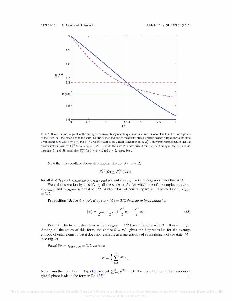
FIG. 2. (Color online) A graph of the average Renyi α-entropy of entanglement as a function of α. The blue line correspondsto the state |M〉, the green line to the state |L〉, the dashed red line to the cluster states, and the dashed purple line to the stategiven in Eq. (33) with θ = π/4. For α ≥ 2 we proved that the cluster states maximize E (α)

2 . However, we conjecture that the

cluster states maximize E (α)2 for α > α0 ≡ 1.59 . . . , while the state |M〉 maximize it for α < α0. Among all the states in M

the state |L〉 and |M〉 minimize E (α)2 for 0 < α < 2 and α > 2, respectively.

Note that the corollary above also implies that for 0 < α < 2,

E (α)2 (ψ) ≤ E (α)

2 (|M〉),

for all ψ ∈ H4 with τ(AB)(C D)(ψ), τ(AC)(B D)(ψ), and τ(AD)(BC)(ψ) all being no greater than 4/3.We end this section by classifying all the states in M for which one of the tangles τ(AB)(C D),

τ(AC)(B D), and τ(AD)(BC) is equal to 3/2. Without loss of generality we will assume that τ(AB)(C D)

= 3/2.

Proposition 15: Let ψ ∈ M. If τ(AB)(C D)(ψ) = 3/2 then, up to local unitaries,

|ψ〉 = 1

2u0 + i

2u1 + eiθ

2u2 + ieiθ

2u3. (33)

Remark: The two cluster states with τ(AB)(C D) = 3/2 have this form with θ = 0 or θ = π/2.Among all the states of this form, the choice θ = π/4 gives the highest value for the averageentropy of entanglement, but it does not reach the average entropy of entanglement of the state |M〉(see Fig. 2).

Proof: From τ(AB)(C D) = 3/2 we have

ψ = 1

2

3∑j=0

eiθ j u j .

Now from the condition in Eq. (16), we get∑3

j=0 ei2θ j = 0. This condition with the freedom ofglobal phase leads to the form in Eq. (33). �


137.207.120.173 On: Wed, 16 Jul 2014 20:39:51


VI. CONCLUSIONS

Four-qubits entanglement is far more complicated to analyse than its three-qubits counterpart.This intricacy manifests itself with the uncountable number of inequivalent SLOCC classes. Suchcomplexity also occur in five- and six-qubits systems, although for these systems there exist max-imally entangled states (such as the five-qubits code state) with the property that any bipartite cutyields a maximally entangled (bipartite) state. Since such states do not exists in four-qubits norin n-qubits with n ≥ 8, the study of four-qubits entanglement gives an insight to the structure ofn-qubits maximally entangled states with large n. Indeed, some of the results presented here, suchas Theorem 5, can be extended to n-qubits.33

In this paper we found an operational interpretation for the 4-tangle as a kind of 4-partyresidual entanglement that can not be shared between two-qubits and two-qubits bipartite cuts.This operational interpretation enabled us to find a family of maximally entangled states that ischaracterized by four real parameters. All the states in the family maximize the average bipartitetangle but only two states in the family (i.e., the states |M〉 and |L〉 in Eqs.(2) and (1)) maximizeall the average Tsillas α-entropy of entanglement. In this sense, up to local unitary transformations,there are only two maximally entangled four-qubits states.

Both the states |M〉 and |L〉 are symmetric; that is, up to local unitaries, they are both invari-ant under permutations of the four-qubits. The eigenvalues of their reduced density matrices thatobtained after tracing out two qubits have the form given in Theorem 8. Therefore, since they bothmaximize the average bipartite tangle, we believe they also optimize many other averages of bipartiteentanglement monotones that were not introduced here. Moreover, the techniques introduced heresuggest that states with the properties of |M〉 and |L〉 may exists in higher dimensional systems.33

We also found that the three cluster states in Eqs. (3), (4), (5) are the only (up to local unitaries)four-qubits states that maximize the average tangle and have the property that out of the three reduceddensity matrices, that obtained by tracing out two qubits, two are proportional to the identity. Inaddition, we showed that the cluster states optimize the average Renyi α-entropy of entanglementwith α ≥ 2. The reason that it is the cluster states and not |M〉 or |L〉 that optimize this averageRenyi entropy is that the Renyi entropy with α ≥ 2 is not concave and so the Renyie entropy ofentanglement is only a deterministic entanglement monotone and not an ensemble monotone.

ACKNOWLEDGEMENTS

The authors are grateful for Ben Fortescue for help with the graphs. G.G. would like to thankDominic Barry, Francesco Buscemi, Ben Fortescue, and Jeong San Kim for fruitful discussions.G.G. research is supported by NSERC.

APPENDIX A: KEMPF–NESS THEOREM

The purpose of this appendix is to state the version of the Kempf–Ness theorem that is used in thispaper. LetHn be n-qubit space and let G be the subgroup SL(2,C) ⊗ SL(2,C) ⊗ · · · ⊗ SL(2,C) (n-copies) in GL(Hn). Let K = SU (2) ⊗ SU (2) ⊗ · · · ⊗ SU (2). Let g be the Lie algebra of G containedin End(Hn). We set Crit(Hn) = {φ ∈ Hn| 〈φ|X |φ〉 = 0, X ∈ g}. The Kempf–Ness theorem in thiscontext says (the only hard part of the theorem is the “if” part of point (3) which we don’t use in thispaper) the following.

Theorem 16: Let φ ∈ Hn then1. φ ∈ Crit(Hn), g ∈ G then ‖gφ‖ ≥ ‖φ‖ with equality if and only if gφ ∈ Kφ,2. if φ ∈ Hn then φ ∈ Crit(Hn) if and only if ‖gφ‖ ≥ ‖φ‖ for all g ∈ G, and3. if φ ∈ Hn then Gφ is closed in Hn if and only if Gφ ∩ Crit(Hn) �= ∅.

We now assume n = 4. Let A be as in Sec. II. Then we obtain the following.

Proposition 17: Crit(H4) = KA.


137.207.120.173 On: Wed, 16 Jul 2014 20:39:51


APPENDIX B: PROOF OF THEOREM 8

We first prove the theorem for the von-Neumann entropy (i.e., the case α = 1) and thenwe will consider the case α �= 1 separately. We want to optimize the function f (λ0, λ1, λ2, λ3)= −∑3

k=0 λk log λk under the constraints∑3

k=0 λk = 1 and∑3

k=0 λ2k = 1 − τ/2, while 0 ≤ λk ≤ 1.

The Lagrangian is therefore given by

L = −3∑

k=0

λk log λk + μ

(3∑

k=0

λk − 1

)+ ν

(3∑

k=0

λ2k + τ

2− 1

),

where μ and ν are the Lagrange multipliers. Therefore, the critical points in the interior of thedomain (i.e., 0 < λk < 1) must satisfy the equation,

∂L∂λk

= − log λk − log e + μ + 2νλk = 0. (B1)

Now, we first show that if all for λk satisfy the equation above, then the set {λk} contains at most twodistinct numbers. To see that, suppose that there are three distinct numbers. Then, without loss ofgenerality, lets assume that λ0 > λ1 > λ2 > 0. Thus, from the three equations above (for k = 0, 1, 2)it follows that

(λ0 − λ1) log λ2 + (λ1 − λ2) log λ0 = (λ0 − λ2) log λ1.

Denote by a ≡ (λ1 − λ2)/(λ0 − λ1). Hence, a > 0 and

log λ2 + a log λ0 = (1 + a) log λ1,

which is equivalent to

λ2λa0 = λ1+a

1 .

Denote by x ≡ λ2/λ1 and y ≡ λ0/λ1. Therefore, x < 1, y > 1, a = (1 − x)/(y − 1), and

xya = 1.

From the last equation and the generalized arithmetic–geometric mean inequality we get

1 = (xya)1/(1+a) ≤ 1

1 + a(x + ay) = 1,

where the last equality is obtained by substituting a = (1 − x)/(y − 1). Note that the geometric–arithmetic mean inequality is saturated if and only if x = y and therefore we get a contradictionto the assumption that there are three distinct numbers in the set {λi }. Therefore, for the interiorpoints we have the following three options: (a) λ0 ≥ λ1 = λ2 = λ3, (b) λ0 = λ1 ≥ λ2 = λ3, and(c) λ0 = λ1 = λ2 ≥ λ3. Option (b) is the only one that does not appear in Theorem 8. In this case

τ must be greater than 1 and λ0 = λ1 = 1+√3x(τ )4 and λ2 = λ3 = 1−√

3x(τ )4 . It is a straightforward

calculation to show that the von-Neumann entropy of this distribution never equals the von-Neumannentropy of the distributions that appear in the theorem. (Note that this is all we have to show since ithas already been proved in Ref. 31 that the distributions in the theorem are the optimal ones).

As for the critical points on the boundary, set λ3 = 0 and then the same argument as aboveimplies that the set {λ0, λ1, λ2} contains at most two distinct numbers. We therefore have twooptions: (a) λ0 = λ1 ≥ λ2 and (b) λ0 ≥ λ1 = λ2. Again, the distribution (b) does not appear inthe theorem, but it is straightforward to show that its von-Neumann entropy never equals to thevon-Neumann entropies of the distributions in the theorem. The last point on the bounday that weneed to check is when λ3 = λ2 = 0, but this distribution appears in the theorem. This completes theproof for the case α = 1.

We now prove the theorem for the case α �= 1 (as well as α �= 2). In this case, we optimize thefunction f (λ0, λ1, λ2, λ3) = ∑3

k=0 λαk under the same constraints above; that is,

∑3k=0 λk = 1 and


137.207.120.173 On: Wed, 16 Jul 2014 20:39:51


∑3k=0 λ2

k = 1 − τ/2. The Lagrangian in this case is given by

L =3∑

k=0

λαk + μ

(3∑

k=0

λk − 1

)+ ν

(3∑

k=0

λ2k + τ

2− 1

),

where μ and ν are the Lagrange multipliers. The critical points in the interior of the domain mustsatisfy the equation,

∂L∂λk

= αλα−1k − log e + μ + 2νλk = 0. (B2)

Similarly to the argument above, we first show that the set {λk} contains at most two distinct numbers.To see that, suppose that there are three distinct numbers λ0 > λ1 > λ2 > 0. Thus, from the threeequations above (for k = 0, 1, 2) it follows that

λα−10 − λα−1

1

λα−10 − λα−1

2

= λ0 − λ1

λ0 − λ2.

Now, denote by x ≡ λ1/λ0 and y ≡ λ2/λ0. From our assumptions 0 < y < x < 1. With thesenotations the equation above can be written as

1 − xα−1

1 − x= 1 − yα−1

1 − y.

However, for nonnegative α �= 2 the function f (x) = (1 − xα−1)/(1 − x) is one-to-one and thereforewe get a contradiction. This complete the proof that the set {λk} contains at most two distinct numbers.The rest of the proof follows the same lines as the proof for the case α = 1.

APPENDIX C: GLOBAL MAX OF f (α)max AND GLOBAL MIN OF f (α)

min

1. Calculation of U(α)

In this section we prove that for α > 2, U (α) = f (α)max(4/3, 4/3, 4/3), and (4/3, 4/3, 4/3) is the

only point of global maximum. Since the function f (α)max(t1, t2, t3) is invariant under permutations of

t1, t2, and t3, we can assume without loss of generality that the global maximum of f (α)max is obtained

at a point with t1 ≥ t2 ≥ t3. We will therefore look for the maximum of f (α)max(t1, t2, 4 − t1 − t2) in

the domain

D ={

(t1, t2)

∣∣∣∣∣43 ≤ t1 ≤ 3

2, 2 − 1

2t1 ≤ t2 ≤ t1

}.

In this domain, t2 can be either bigger or smaller than 4/3 and therefore the derivative of f (α)max with

respect to t2 is not continuous at points with t2 = 4/3. We therefore split the domain D into tworegions,

D1 ={

(t1, t2)

∣∣∣∣∣43 ≤ t1 ≤ 3

2,

4

3≤ t2 ≤ t1

},

D2 ={

(t1, t2)

∣∣∣∣∣43 ≤ t1 ≤ 3

2, 2 − 1

2t1 ≤ t2 ≤ 4

3

},

so that on D1 (or D2) all the derivatives of f (α)max are continuous. We start by maximizing f (α)

max on thedomain D1.


137.207.120.173 On: Wed, 16 Jul 2014 20:39:51


1. Maximizing f (α)max on the domain D1

Denote by xi =√

1 − 23 ti , for i = 1, 2, and y =

√1 − 3

4 t3. In these variables, the function

g(α)max(x1, x2) ≡ f (α)

max(t1, t2, 4 − t1 − t2) is given by

g(α)max(x1, x2) = 1

α − 1

[1 −

∑i=1,2

((1 + xi )α

4α+ 1

3

(1 − 3xi )α

4α

)

− 2

3α+1(1 + y)α − 1

3α+1(1 − 2y)α

],

where in term of the variables x1 and x2, y = 12

√1 − 9

2 (x21 + x2

2 ). In terms of these new variables, thedomain D1 is given by 0 ≤ x1 ≤ x2 ≤ 1/3. We start by looking at the critical points in the interiorof D1.

The critical points of g(α)max(x1, x2) satisfies the conditions,

∂g(α)max

∂x1(x1, x2) = x1

4(uα(y) − vα(x1)) = 0,

∂g(α)max

∂x2(x1, x2) = x2

4(uα(y) − vα(x2)) = 0,

where

vα(x) ≡ α

(α − 1)4α−1

1

x

[(1 + x)α−1 − (1 − 3x)α−1] ,

uα(y) ≡ α

(α − 1)3α−1

1

y

[(1 + y)α−1 − (1 − 2y)α−1

].

Hence, the point (x1, x2) is critical if and only if vα(x1) = vα(x2) = uα(y), where y

= 12

√1 − 9

2 (x21 + x2

2 ) (note that 0 ≤ y ≤ 1/2). In the next two lemmas we prove two useful proper-ties of the functions vα(x) and uα(y).

Lemma 18: If 2 < α < 4, and 0 ≤ y ≤ 1/2, then u′α(y) < 0. If 2 < α < 5, and 0 ≤ x ≤ 1/3,

then v′α(x) < 0.

Proof: A simple calculation gives

u′α(y) = α

(α − 1)3α−1

1

y2

[(1 + y)β (βy − 1) + (1 − 2y)β (1 + 2βy)

],

where β ≡ α − 2. From the assumption of the lemma 0 < β < 2. Therefore, one can easily checkthat u′

α(0) < 0 and u′α(1/2) < 0. All that is left to show is that in the domain 0 < y < 1/2, the

function

w(y) ≡ (1 + y)β(βy − 1) + (1 − 2y)β(1 + 2βy)

is negative. To find its maximum value, we calculate its critical points. The requirement w′(y) = 0gives (1 + y)β−1 = 4(1 − 2y)β−1. Clearly, there are no critical points for β ≤ 1 in the domain(0, 1/2). For β > 1 we express the value of w(yc) at the critical point by substituting for (1 + yc)β−1

the value 4(1 − 2yc)β−1. This gives,

w(yc) = −3(1 − 2yc)β−1 [1 − 2(β − 1)yc] < 0,


137.207.120.173 On: Wed, 16 Jul 2014 20:39:51


for yc < 1/2 and β < 2. Hence, u′α(y) < 0 for 2 < α < 4. Following the same arguments, one can

show that v′α(x) < 0 for 2 < α < 5. �

Lemma 19: If α ≥ 4 then the global maximum of vα(x) (in the domain 0 ≤ x ≤ 1/3) is strictlysmaller than the global minimum of the function uα(y) (in the domain 0 ≤ y ≤ 1/2).

Proof: The global extremum points of uα and vα are obtained on the boundary or on criticalpoints. Therefore, we first check the bounday (that is, end points). We have

vα(0) = α

4α−2, vα

(1

3

)= α

α − 1

1

3α−2

uα(0) = α

3α−2, uα

(1

2

)= α

α − 1

1

2α−2

Clearly, for α ≥ 4, we have max{vα(0), vα(1/3)} < min{uα(0), uα(1/2)}. We now estimate the valuesof uα and vα at their critical points xc and yc. From u′

α(yc) = 0 and v′α(xc) = 0 we have

uα(yc) = α

3α−1

[(1 + yc)α−2 + 2(1 − 2yc)α−2

],

vα(xc) = α

4α−1

[(1 + xc)α−2 + 3(1 − 3xc)α−2] . (C1)

Since we do not have explicit expressions for xc and yc, we find an upper bound for vα(xc) and alower bound for uα(yc). Since the functions in Eq. (C1) are convex for α ≥ 4, we get

vα(xc) ≤ max{vα(xc = 0), vα(xc = 1/3)}

= max{1

4

α

3α−2,

α

4α−2

}.

The minimum value of the function uα(yc) given in Eq. (C1) is obtained at the point

yc = 41/(α−3) − 1

1 + 2 · 41/(α−3).

Note that this is not necessarily the true value of yc, but rather the value at which the function inEq. (C1) is minimized. It is a straightforward calculation to show that at this value of yc

uα(yc) > max

{1

4

α

3α−2, vα(0) , vα(1/3)

}.

This completes the proof that uα(y) > vα(x) for α ≥ 4 and for all x ∈ [0, 1/3] and y ∈ [0, 1/2]. �From Lemma 19 it follows that for α ≥ 4 the function g(α)

max(x1, x2) does not have critical pointsin the interior of D1. For 2 < α < 4, g(α)

max(x1, x2) can have critical points. However, from the secondderivatives test and from Lemma 18, it follows that the Hessian is positive definite. Therefore, thesecritical points are local min and can not be a global max. The global maximum of g(α)

max(x1, x2) istherefore obtained at the boundary of D1.

The boundary of D1 is a triangle with three sides given by x1 = 0, x1 = x2, and x2 = 1/3. Ifx1 = 0 then

dg(α)max(0, x2)

dx2= x2

4(uα(y) − vα(x2)) .

Therefore, g(α)max(0, x2) is convex for 2 < α < 4 (see Lemma 18) and has no critical points for α ≥ 4

(see Lemma 19). Therefore, its global max is obtained at one of the end points (0, 0) or (0, 1/3).On the side x1 = x2 ≡ x we have

d

dxg(α)

max(x, x) = x

2(uα(y) − vα(x)) .

Hence, the same arguments implies that the global max of g(α)max(x, x) is obtained at one of

the end points x = 0 or x = 1/3. Similarly, on the side x2 = 1/3, the function g(α)max(x1, 1/3)


137.207.120.173 On: Wed, 16 Jul 2014 20:39:51


obtains its global maximum at one of the end points x1 = 0 or x1 = 1/3. Among the three ver-tices (0, 0), (0, 1/3), (1/3, 1, 3), we have

g(α)max(1/3, 1/3) > max

{g(α)

max(0, 0) , g(α)max(0, 1/3)

}for all α > 2. Hence, on D1, g(α)

max obtains its global max at the point (x1, x2) = (1/3, 1/3) which isequivalent to t1 = t2 = t3 = 4/3.

2. Maximizing f (α)max on the domain D2

Denote by x =√

1 − 23 t1 and yi =

√1 − 3

4 ti for i = 2, 3 . In these variables, the function

h(α)max(y2, y3) ≡ f (α)

max(4 − t2 − t3, t2, t3) is given by

h(α)max(y2, y3) = 1

α − 1

[1 − 2

3α+1

∑i=2,3

((1 + yi )

α − 1

2(1 − 2yi )

α

)

− 1

4α

((1 + x)α + 1

3(1 − 3x)α

)],

where in term of the variables y2 and y3, x = 13

√1 − 8(y2

2 + y23 ). In terms of these new variables,

the domain D2 is therefore given by

D2 ={

(y2, y3)∣∣∣y2

2 + y23 ≤ 1

8, y3 ≥ y2 ≥ 0

}.

We first look at the critical points in the interior of D2.The critical points of h(α)

max(y2, y3) satisfies the conditions

∂h(α)max

∂y2(y2, y3) = 2y2

9(vα(x) − uα(y2)) = 0,

∂h(α)max

∂y3(y2, y3) = 2y3

9(vα(x) − uα(y3)) = 0.

Hence, it follows from Lemmas 18 and 19 that the global max of h(α)max(y2, y3) is obtained on the

boundary of D2.The boundary of D2 consists of the line y2 = 0, the line y1 = y2, and the curve (y2, y3)

= (sin θ/√

8, cos θ/√

8) with 0 ≤ θ ≤ π/4. The global maximum of h(α)max on the lines y2 = 0 and

y1 = y2 is obtained on one of the endpoints (0, 1/2), (0, 0), and (1/4, 1/4). The argument followsfrom Lemmas 18 and 19, in the same way as it was used in the analysis of the boundary of D1.Therefore, we focus now on the curve (y2, y3) = (sin θ/

√8, cos θ/

√8) with 0 ≤ θ ≤ π/4.

Let

h(θ ) ≡ h(α)max

(sin θ√

8,

cos θ√8

).

Note that for these values of y2 and y3, x = 0. Hence,

h′(θ ) = sin(2θ )

72

[uα

(cos θ√

8

)− uα

(sin θ√

8

)].

From Lemma 18 the function uα is one-to-one for 2 < α < 4. Therefore, the only critical point inthis case is (y2, y3) = (1/4, 1/4). For α ≥ 4 it is a simple calculation to verify that h(θ ) < h(α)

max(0, 0).Therefore, since

h(α)max(0, 0) > max

{h(α)

max(1/4, 1/4), h(α)max(0, 1/2)

}for all α > 2, we conclude that on D2, h(α)

max obtains its global max at the point (y1, y2) = (0, 0)which is equivalent to t1 = t2 = t3 = 4/3.


137.207.120.173 On: Wed, 16 Jul 2014 20:39:51


2. Calculation of L(α)

In this section we prove that for 0 < α < 2, L (α) = f (α)min(4/3, 4/3, 4/3) and (4/3, 4/3, 4/3) is

the only point of global minimum. From Theorem 8 it follows that f (α)min(t1, t2, t3) for 0 < α < 2

is given by the exact same expression as f (α)max(t1, t2, t3) for α > 2. Therefore, our proof that L (α)

= f (α)min(4/3, 4/3, 4/3) follows the exact same steps used in the calculation of U (α) for α > 2. The

only difference is that the Lemmas 18 and 19 do not hold for 0 < α < 2, and instead we have thefollowing lemma.

Lemma 20: If 0 < α < 2, 0 ≤ x ≤ 1/3, and 0 ≤ y ≤ 1/2, then u′α(y) > 0 and v′

α(x) > 0.

Proof: A simple calculation gives

u′α(y) = α

(α − 1)3α−1

1

y2

[(1 + 2βy)

(1 − 2y)β− (1 + βy)

(1 + y)β

],

where β ≡ 2 − α. From the assumption of the lemma 0 < β < 2. Therefore, one can easily checkthat limy→0 u′

α(y) > 0 and limy→1/2 u′α(y) = +∞. All that is left to show is that in the domain

0 < y < 1/2 the function

w(y) ≡ 1

(1 − β)

1

y2

[(1 + 2βy)

(1 − 2y)β− (1 + βy)

(1 + y)β

]

is positive. To find its minimum value, we would like to calculate its critical points. However, therequirement w′(y) = 0 gives 4(1 + y)β+1 = (1 − 2y)β+1. Hence, there are no critical points in thedomain (0, 1/2). That is, u′

α(y) > 0 for 0 < α < 2. Following the same arguments, one can showthat v′

α(x) > 0 for 0 < α < 2. �With this lemma replacing lemmas 18 and 19, the proof that L (α) = f (α)

min(4/3, 4/3, 4/3) followsexactly the same steps that appear in the calculation of U (α).

1 E. Schrdinger, Math. Proc. Cambridge Philos. Soc. 31, 555 (1935).2 C. H. Bennett, G. Brassard, C. Crepeau, R. Jozsa, A. Peres, and W. K. Wootters, Phys. Rev. Lett. 70, 1895 (1993).3 C. H. Bennett and S. J. Wiesner, Phys. Rev. Lett. 69, 2881 (1992).4 R. Horodecki, P. Horodecki, M. Horodecki, and K. Horodecki, Rev. Mod. Phys. 81, 865 (2009).5 M. B. Plenio and S. Virmani, Quantum Inf. Comput. 7, 1 (2007).6 H. J. Briegel and R. Raussendorf, Phys. Rev. Lett. 86, 910 (2001); R. Raussendorf and H. J. Briegel, ibid. 86, 5188 (2001).7 P. Walther et al., Nature (London) 434, 169 (2005); R. Prevedel et al., Nature (London) 445, 65 (2007); C.-Y. Lu et al.,

Nat. Phys. 3, 91 (2007); M. S. Tame et al., Phys. Rev. Lett. 98, 140501 (2007); K. Chen et al., Phys. Rev. Lett. 99, 120503(2007).

8 D. Schlingemann and R. F. Werner, Phys. Rev. A 65, 012308 (2001).9 R. Cleve, D. Gottesman, and H.-K. Lo, Phys. Rev. Lett. 83, 648 (1999).

10 G. Gour and N. R. Wallach, Phys. Rev. A 76, 042309 (2007).11 W. Dr, G. Vidal, and J. I. Cirac, Phys. Rev. A 62, 062314 (2000).12 C. H. Bennett et al., Phys. Rev. A 54, 3824 (1996); R. Laflamme et al., Phys. Rev. Lett. 77, 198 (1996).13 E. Rains, IEEE Trans. Inf. Theory 45, 266 (1999).14 P. J. Love et al., Quantum Inf. Process. 6, 187 (2007).15 A. J. Scott, Phys. Rev. A. 69, 052330 (2004).16 A. Osterloh and J. Siewert, Phys. Rev. A. 72, 012337 (2005); D. Z. Dokovic and A. Osterloh, J. Math. Phys. 50, 033509

(2009); A. Osterloh and J. Siewert, e-print arXiv:quant-ph/0908:3818.17 A. Higuchi and A. Sudbery, Phys. Lett. A 273, 213 (2000).18 S. Brierley and A. Higuchi, J. Phys. A: Math. Theor. 40, 8455 (2007).19 G. Gour, S. Bandyopadhyay, and B. C. Sanders, J. Math. Phys. 48, 012108 (2007).20 N. R. Wallach, Lectures on Quantum Computing (C.I.M.E., Venice, 2004). See http://www.math.ucsd.edu/

nwallach/venice.pdf.21 F. Verstraete, J. Dehaene, B. De Moor, and H. Verschelde, Phys. Rev. A 65, 052112 (2002).22 F. Verstraete, J. Dehaene, and B. De Moor, Phys. Rev. A 68, 052112 (2003).23 G. Gour, Phys. Rev. A 71, 012318 (2005).24 G. Kempf and L. Ness, The Length of Vectors in Representation Spaces, Lecture Notes in Mathematics Vol. 732 (Springer,

Berlin, 1979), pp. 233–243.25 A. Klyachko, arXiv:quant-ph/0206012.26 V. Coffman, J. Kundu, and W. K. Wootters, Phys. Rev. A 61, 052306 (2000).27 A. Uhlmann, Phys. Rev. A 62, 032307 (2000); A. Wong and N. Christensen, ibid. 63, 044301 (2001); S. S. Bullock and

G. K. Brennen, J. Math. Phys. 45, 2447 (2004).28 J.-G. Luque and J.-Y. Thibon, Phys. Rev. A 67, 042303 (2003).


137.207.120.173 On: Wed, 16 Jul 2014 20:39:51

http://dx.doi.org/10.1017/S0305004100013554

http://dx.doi.org/10.1103/PhysRevLett.70.1895


http://dx.doi.org/10.1103/RevModPhys.81.865


http://dx.doi.org/10.1038/nature03347

http://dx.doi.org/10.1103/PhysRevA.65.012308





http://dx.doi.org/10.1109/18.746807

http://dx.doi.org/10.1007/s11128-007-0052-7



http://dx.doi.org/10.1016/S0375-9601(00)00480-1

http://dx.doi.org/10.1088/1751-8113/40/29/018

http://dx.doi.org/10.1063/1.2435088








29 Xinhua Hu and Zhongxing Ye, J. Math. Phys. 47, 023502 (2006).30 W. V. Dam and P. Hayden, e-print arXiv:quant-ph/0204093.31 D. W. Berry and B. C. Sanders, J. Phys A 36, 12255 (2003).32 Dominic W. Berry, private communication.33 G. Gour and N. Wallach, (to be published).34 Note that f0 is the G-concurrence23 between qubits (1,2) and (3,4).35 A state ψ is stable if the set of states Gψ is closed in H4.36 We are willing to conjecture that it is true for all α ≥ 0.


137.207.120.173 On: Wed, 16 Jul 2014 20:39:51

http://dx.doi.org/10.1063/1.2165794

http://dx.doi.org/10.1088/0305-4470/36/49/008

Documents

All maximally entangled four-qubit states