Embed Size (px)
Citation preview

Algorithms for Web Scraping
Patrick Hagge Cording
Kongens Lyngby 2011

Technical University of DenmarkDTU InformaticsBuilding 321, DK-2800 Kongens Lyngby, DenmarkPhone +45 45253351, Fax +45 [email protected]
Abstract
Web scraping is the process of extracting and creating a structured representa-tion of data from a web site. HTML, the markup language used to structuredata on webpages, is subject to change when for instance the look-and-feel isupdated. Since current techniques for web scraping are based on the markup, achange may lead to the extraction of incorrect data.
In this thesis we investigate the potential of using approximate tree patternmatching based on the tree edit distance and constrained derivatives for webscraping. We argue that algorithms for constrained tree edit distances are notsuited for web scraping. To address the high time complexity of optimal treeedit distance algorithms, we present the lower bound pruning algorithm which,based on the data tree TD and the pattern tree TP , will attempt to removebranches of TD that are not part of an optimal mapping. Its running timeis O
(|TD||TP | · σ(TD, TP )
), where σ(TD, TP ) is the running time of the lower
bound method used. Although it asymptotically is close to the approximate treepattern matching algorithms, we show that in practice the total execution timeis reduced in some cases. We develop several methods for determining a lowerbound on the tree edit distance used for approximate tree pattern matching,and we see that our generalization of the q-gram distance from strings is themost effective with our algorithm. We also present a similar algorithm that usethe HTML grammar to prune TD, and some heuristics to guide the approximatetree pattern matching algorithm.

ii
Preface
This master’s thesis has been prepared at DTU Informatics from february 2011to august 2011 under supervision by associate professors Inge Li Gørtz andPhilip Bille. It has an assigned workload of 30 ECTS credits.
Source code for the software developed for the thesis is available from the fol-lowing two mirrors.
http://www.student.dtu.dk/˜s062408/scpx.ziphttp://iscc-serv2.imm.dtu.dk/˜patrick/scpx.zip
Acknowledgements. I would like to thank my supervisors for always beingenthusiastic at our meetings. The individuals who have influenced my workinclude Henrik and Anne-Sofie of Kapow Software who took time out of theirschedule to discuss web scraping, my friend Christoffer who brought my atten-tion to the challenges faced in web scraping, friend and co-student Kristofferwho wrapped his head around the project in order to give criticism, and mygirlfriend who has provided proof-reading. I am grateful to all.
Patrick Hagge Cording

iv

Contents
Abstract i
Preface iii
1 Introduction 11.1 Preliminaries and Notation . . . . . . . . . . . . . . . . . . . . . 2
2 Tree Edit Distance 52.1 Problem Definition . . . . . . . . . . . . . . . . . . . . . . . . . . 52.2 Algorithms . . . . . . . . . . . . . . . . . . . . . . . . . . . . . . 82.3 Constrained Mappings . . . . . . . . . . . . . . . . . . . . . . . . 122.4 Approximate Tree Pattern Matching . . . . . . . . . . . . . . . . 15
3 Web Scraping using Approximate Tree Pattern Matching 173.1 Basic Procedure . . . . . . . . . . . . . . . . . . . . . . . . . . . 173.2 Pattern Design . . . . . . . . . . . . . . . . . . . . . . . . . . . . 193.3 Choosing an Algorithm . . . . . . . . . . . . . . . . . . . . . . . 213.4 Extracting Several Matches . . . . . . . . . . . . . . . . . . . . . 223.5 Related Work . . . . . . . . . . . . . . . . . . . . . . . . . . . . . 223.6 Summary . . . . . . . . . . . . . . . . . . . . . . . . . . . . . . . 24
4 Lower Bounds for Tree Edit Distance with Cuts 254.1 Tree Size and Height . . . . . . . . . . . . . . . . . . . . . . . . . 254.2 Q-gram Distance . . . . . . . . . . . . . . . . . . . . . . . . . . . 264.3 PQ-gram Distance . . . . . . . . . . . . . . . . . . . . . . . . . . 284.4 Binary Branch Distance . . . . . . . . . . . . . . . . . . . . . . . 294.5 Euler String Distance . . . . . . . . . . . . . . . . . . . . . . . . 324.6 Summary . . . . . . . . . . . . . . . . . . . . . . . . . . . . . . . 35
vi CONTENTS
5 Data Tree Pruning and Heuristics 375.1 Adapting the Fast Unit Cost Algorithm to Cuts . . . . . . . . . . 375.2 Using Lower Bounds for Pruning . . . . . . . . . . . . . . . . . . 415.3 Using the HTML Grammar for Pruning . . . . . . . . . . . . . . 445.4 Pre-selection of Subtrees . . . . . . . . . . . . . . . . . . . . . . . 465.5 Linear Matching . . . . . . . . . . . . . . . . . . . . . . . . . . . 47
6 Experiments 496.1 Setup . . . . . . . . . . . . . . . . . . . . . . . . . . . . . . . . . 496.2 Algorithm Execution Time . . . . . . . . . . . . . . . . . . . . . 506.3 Lower Bound Methods . . . . . . . . . . . . . . . . . . . . . . . . 516.4 Pruning Methods . . . . . . . . . . . . . . . . . . . . . . . . . . . 516.5 Heuristics . . . . . . . . . . . . . . . . . . . . . . . . . . . . . . . 546.6 Data Extraction . . . . . . . . . . . . . . . . . . . . . . . . . . . 58
7 Discussion 637.1 Algorithms . . . . . . . . . . . . . . . . . . . . . . . . . . . . . . 637.2 Lower Bound Methods . . . . . . . . . . . . . . . . . . . . . . . . 647.3 Pruning Method and Heuristics . . . . . . . . . . . . . . . . . . . 65
8 Conclusion 678.1 Further Work . . . . . . . . . . . . . . . . . . . . . . . . . . . . . 68
Bibliography 69
A Implementation 73A.1 Design . . . . . . . . . . . . . . . . . . . . . . . . . . . . . . . . . 73A.2 Modules . . . . . . . . . . . . . . . . . . . . . . . . . . . . . . . . 74A.3 Examples . . . . . . . . . . . . . . . . . . . . . . . . . . . . . . . 79
B Algorithms 83B.1 Algorithm for finding Q-grams . . . . . . . . . . . . . . . . . . . 83B.2 Algorithm for finding Q-samples . . . . . . . . . . . . . . . . . . 83
C Test Case Patterns 85C.1 Case 1 . . . . . . . . . . . . . . . . . . . . . . . . . . . . . . . . . 85C.2 Case 2 . . . . . . . . . . . . . . . . . . . . . . . . . . . . . . . . . 87C.3 Case 3 . . . . . . . . . . . . . . . . . . . . . . . . . . . . . . . . . 88C.4 Case 4 . . . . . . . . . . . . . . . . . . . . . . . . . . . . . . . . . 89C.5 Case 5 . . . . . . . . . . . . . . . . . . . . . . . . . . . . . . . . . 90C.6 Case 6 . . . . . . . . . . . . . . . . . . . . . . . . . . . . . . . . . 90

List of Figures
2.1 Example insert, delete, and relabel operations. . . . . . . . . . . . 62.2 An example of a mapping. . . . . . . . . . . . . . . . . . . . . . . 72.3 An example of a top-down mapping. . . . . . . . . . . . . . . . . 132.4 An example of an isolated-subtree mapping. . . . . . . . . . . . . 142.5 The effect from introducing the cut operation. . . . . . . . . . . . 15
(a) A mapping between a large and small tree. . . . . . . . . . 15(b) A mapping using the tree edit distance with cuts. . . . . . 15
3.1 A HTML document and its tree model. . . . . . . . . . . . . . . 183.2 A selection of entries from the frontpage of Reddit (2011-06-25). . 193.3 A pattern for a Reddit entry and its tree model. . . . . . . . . . 203.4 A pattern with an anchor for a Reddit entry and its tree model. . 203.5 Example of the difference in outcome from using an original map-
ping and an isolated-subtree mapping. . . . . . . . . . . . . . . . 23(a) A Reddit entry before the change. Subtree is used as pattern. 23(b) A Reddit entry after the change. . . . . . . . . . . . . . . . 23(c) The optimal mapping as produced by e.g. Zhang and Shasha’s
algorithm. . . . . . . . . . . . . . . . . . . . . . . . . . . . . 23(d) The isolated-subtree mapping. . . . . . . . . . . . . . . . . 23
4.1 An example of a tree extended for the PQ-gram distance. . . . . 29(a) T . . . . . . . . . . . . . . . . . . . . . . . . . . . . . . . . . 29(b) T 2,2, the 2,2-extension of T . . . . . . . . . . . . . . . . . . . 29
4.2 An example of a binary tree representation. . . . . . . . . . . . . 30(a) T . . . . . . . . . . . . . . . . . . . . . . . . . . . . . . . . . 30(b) The binary tree representation of T . . . . . . . . . . . . . . 30
4.3 An example of 1,2-grams affected by a delete operation on a tree. 31(a) T . . . . . . . . . . . . . . . . . . . . . . . . . . . . . . . . . 31

viii LIST OF FIGURES
(b) T after deleting b. . . . . . . . . . . . . . . . . . . . . . . . 31(c) Binary tree representation of T . . . . . . . . . . . . . . . . 31(d) Binary tree representation of T after deleting b. . . . . . . . 31
4.4 A tree and its Euler string. . . . . . . . . . . . . . . . . . . . . . 33
5.1 A problem which shows that keyroots can not be used with theunit cost algorithm. . . . . . . . . . . . . . . . . . . . . . . . . . 39
5.2 A possible solution path to a subproblem in the temporary dy-namic programming table in Zhang and Shasha’s algorithm. . . . 40
5.3 Comparison of how subproblems are ruled out in the permanentand temporary table of Zhang and Shasha’s algorithms. . . . . . 42(a) Algorithm using keyroots. . . . . . . . . . . . . . . . . . . . 42(b) Fast unit cost algorithm. . . . . . . . . . . . . . . . . . . . 42(c) Fast unit cost algorithm adapted for cuts. . . . . . . . . . . 42
5.4 Division into subforests for computing improved lower boundwhen pruning. . . . . . . . . . . . . . . . . . . . . . . . . . . . . . 44
6.1 Execution time of lower bound pruning methods followed by Zhang-ShashaATM on case 1 for increasing values of k. . . . . . . . . . 57
6.2 Execution time of lower bound pruning methods followed by Zhang-ShashaATM on case 3 for increasing values of k. . . . . . . . . . 57
6.3 Initial layout of web page used for data extraction experiment. . 596.4 Results from data extraction experiment (part 1). . . . . . . . . . 61
(a) . . . . . . . . . . . . . . . . . . . . . . . . . . . . . . . . . 61(b) . . . . . . . . . . . . . . . . . . . . . . . . . . . . . . . . . 61(c) . . . . . . . . . . . . . . . . . . . . . . . . . . . . . . . . . 61(d) . . . . . . . . . . . . . . . . . . . . . . . . . . . . . . . . . 61
6.5 Results from data extraction experiment (part 2). . . . . . . . . . 62(e) . . . . . . . . . . . . . . . . . . . . . . . . . . . . . . . . . 62(f) . . . . . . . . . . . . . . . . . . . . . . . . . . . . . . . . . 62(g) . . . . . . . . . . . . . . . . . . . . . . . . . . . . . . . . . 62(h) . . . . . . . . . . . . . . . . . . . . . . . . . . . . . . . . . 62
A.1 Class diagram. . . . . . . . . . . . . . . . . . . . . . . . . . . . . 75
List of Tables
3.1 The number of nodes and the height of the DOM trees of selectedweb sites (2011-07-17). . . . . . . . . . . . . . . . . . . . . . . . . 21
4.1 Preprocessing, space, and time requirements of the lower boundsmethods. . . . . . . . . . . . . . . . . . . . . . . . . . . . . . . . . 35
6.1 Test cases used for experiments. . . . . . . . . . . . . . . . . . . . 506.2 Execution times of Zhang and Shasha’s approximate tree pattern
matching algorithm. . . . . . . . . . . . . . . . . . . . . . . . . . 516.3 Shasha and Zhang’s fast unit cost algorithm adapted for cuts on
all test cases for increasing values of k. . . . . . . . . . . . . . . . 526.4 Results for lower bounds test. . . . . . . . . . . . . . . . . . . . . 526.5 Results for alternative lower bounds test. . . . . . . . . . . . . . 536.6 Results from pruning method tests. . . . . . . . . . . . . . . . . . 556.7 Results from combining two pruning methods. . . . . . . . . . . . 566.8 Results from using the heuristics with ZhangShashaATM. . . . 58
A.1 List of algorithm implementations. . . . . . . . . . . . . . . . . . 76

x LIST OF TABLES

Chapter 1
Introduction
Web scraping is the process of extracting and creating a structured representa-tion of data from a web site. A company may for instance want to autonomouslymonitor its competitors product prices, or an enterprising student may want tounify information on parties from all campus bar and dormitory web sites andpresent them in a calendar on her own web site.
If the owner of the information does not provide an open API, the remedy is towrite a program that targets the markup of the web page. A common approach isto parse the web page to a tree representation and evaluate an XPath expressionon it. An XPath denotes a path, possibly with wildcards, and when evaluatedon a tree, the result is the set of nodes at the end of any occurence of the path inthe tree. HTML, the markup language used to structure data on web pages, isintended for creating a visually appealing interface for humans. The drawbackof the existing techniques used for web scraping is that the markup is subjectto change either because the web site is highly dynamic or simply because thelook-and-feel is updated. Even XPaths with wildcards are vulnerable to thesechanges because a given change may be to a tag which can not be covered by awildcard.
In this thesis we show how to perform web scraping using approximate treepattern matching. A commonly used measure for tree similarity is the tree editdistance which easily can be extended to be a measure of how well a pattern

2 Introduction
can be matched in a tree. An obstacle for this approach is its time complexity,so we consider if faster algorithms for constrained tree edit distances are usablefor web scraping, and we develop algorithms and heuristics to reduce the size ofthe tree representing the web page.
The aim of the project is to a develop a solution for web scraping that is
• tolerant towards as many changes in the markup as possible,
• fast enough to be used in e.g. a web service where response time is crucial,and
• pose no constraints on the pattern, i.e. any well-formed HTML snippetshould be usable as pattern.
The rest of the report is organized as follows. Chapter 2 is a subset of the the-ory of the tree edit distance. We accentuate parts that have relevance to webscraping. In chapter 3 we describe how approximate tree pattern matching isused for web scraping and we discuss pros and cons of the algorithms mentionedin chapter 2. In chapter 4 we transform six techniques for approximation of thetree edit distance to produce lower bounds for the pattern matching measure.Chapter 5 presents an algorithm that uses the lower bound methods from chap-ter 4 to prune the data tree. We also present an algorithm and two heuristicsthat use knowledge of HTML to reduce the tree. In chapter 6 we conduct someexperiments and chapter 7 is a discussion of our results.
Appendix A describes the software package developed for the thesis. It gives abrief overview of the design of the package and contains examples of how to useit.
1.1 Preliminaries and Notation
1.1.1 General
It is assumed that the reader has basic knowledge of HTML, is familiar withthe string edit distance problem, and the concept of dynamic programming.
We use Smallcaps when referring to algorithms that have been implemented ordescribed using pseudocode. Typewriter is used for URL’s as well as modules

1.1 Preliminaries and Notation 3
and functions in the implementation chapter. Likewise, serif is used to refer toclasses.
For pseudocode we use ← for assignment and = for comparison. We do notdistinguish lists and sets. The union of two lists is the set of elements in theconcatenation of the lists, e.g. [x, y] ∪ [x, x, z] = [x, y, z]. We use ⊕ to denoteconcatenation, e.g. [x, y] ⊕ [x, x, z] = [x, y, x, x, z]. A tuple is a list of fixedlength. We use round parenthesis for tuples to distinguish them from lists. Theconcatenation operator also applies to tuples. The length of a list or tuple a is|a|.
1.1.2 Trees and Forests
T denotes a tree and F denotes a forest. Trees and forests are rooted andordered if nothing else is stated. |T | is the size of the tree T . V (T ) is the set ofall nodes in T . T (v) is the subtree rooted at the node v and F (v) is the forestobtained from removing v from T (v). When nothing else is stated the nodes areassigned postorder indices. Any arithmetic operation on two nodes is implicitlyon their indices and the result is a number. T [i] is the ith node in T . The ‘−’operator on a tree and a node removes a subtree or a node from a tree, e.g.T − T (v) removes the subtree rooted at v from T . The empty forest is denotedθ.
We define the following functions on trees.
root : T → V (T ). Returns the root of the tree given as input.
height : V (T )→ Z. Computes the height of the subtree rooted at the node givenas input.
depth : V (T )→ Z. Returns the length of the path from the root of T to givennode.
lml : V (T )→ V (T ). Finds the leftmost leaf of the tree rooted at the node givenas input.
nca : V (T )× V (T )→ V (T ). Finds the nearest common ancestor of the nodes.
leaves : T → Z. Returns the number of leaves in the tree.
degree : T → Z. Computes the max number of children of all nodes in T .

4 Introduction
For simplicity we sometimes give a tree as input to a function expecting a node.In such cases the root of the tree is implicitly the input.
Finally, we define the anchor of a tree T as path p from the root of T to somenode v where each node on p has exactly one child and v is either a leaf or hasmore than one child. If the root has more than one child, the length of theanchor is 1.

Chapter 2
Tree Edit Distance
In this chapter we review the theory of the tree edit distance which is neededfor the rest of the thesis.
2.1 Problem Definition
Definition 2.1 (Tree Edit Distance) Let T1 and T2 be rooted, ordered treesand let E = op0, op1, . . . , opk be an edit script (a sequence of operations on thetrees) that transforms T1 into T2. Let γ be a cost function on operations, thenthe cost of an edit script is
∑k−1i=0 γ(opi). The tree edit distance δ(T1, T2) is the
cost of a minimum cost edit script.
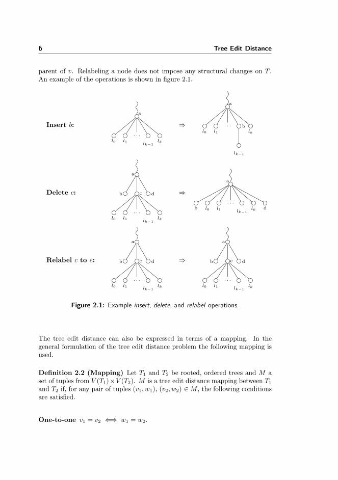
The tree edit distance problem is to compute the tree edit distance and itscorresponding edit script. In the general formulation of the problem, the editoperations are insert, delete, and relabel. A node v can be inserted anywherein T . When inserted as the root, the old root becomes a child of v. If insertedbetween two nodes u and w, v takes the place of w in the left-to-right orderof the children of u, and w becomes the only child of v. A node can also beinserted as a leaf. When deleting a node v, its children become children of the
6 Tree Edit Distance
parent of v. Relabeling a node does not impose any structural changes on T .An example of the operations is shown in figure 2.1.
Insert b:
a
l0 l1
. . .
lk−1lk
⇒
a
l0 l1
. . . b
lk−1
lk
Delete c:
a
b c
l0 l1
. . .
lk−1lk
d ⇒
a
b l0 l1
. . .
lk−1lk d
Relabel c to e:
a
b c
l0 l1
. . .
lk−1lk
d ⇒
a
b e
l0 l1
. . .
lk−1lk
d
Figure 2.1: Example insert, delete, and relabel operations.
The tree edit distance can also be expressed in terms of a mapping. In thegeneral formulation of the tree edit distance problem the following mapping isused.
Definition 2.2 (Mapping) Let T1 and T2 be rooted, ordered trees and M aset of tuples from V (T1)×V (T2). M is a tree edit distance mapping between T1
and T2 if, for any pair of tuples (v1, w1), (v2, w2) ∈M , the following conditionsare satisfied.
One-to-one v1 = v2 ⇐⇒ w1 = w2.

2.1 Problem Definition 7
Ancestor v1 is an ancestor of v2 ⇐⇒ w1 is an ancestor of w2.
Sibling v1 is to the left of v2 ⇐⇒ w1 is to the left of w2.
Mappings and edit scripts are interchangeable. A pair of nodes (v, w) ∈ Mcorresponds to relabeling v to w. Any node in T1 that is not in any tuplein M should be deleted, and any node in T2 that is not in any tuple in Mshould be inserted. So if an edit script creates a mapping that violates one ofthe three conditions, it is not a solution to the tree edit distance problem. Anexample of a mapping is shown in figure 2.2. Intuitively, the mapping conditionsare formalizations of what makes trees similar. If they are relaxed, the treeedit distance will no longer correspond to what we believe is similarity betweentrees. If they are augmented, the tree edit distance will correspond to a differentperception of similarity between trees, and the complexity of computing it maybe reduced.
a
b
d e
c
f g
a
de
h
i
f g
Figure 2.2: A mapping that corresponds to the edit script relabel(a,a),delete(b), insert(h), relabel(c,i), relabel(d,d), relabel(e,e), relabel(f,f), re-label(g,g). We usually omit relabel operations in the edit script if theircost is zero, but they are included here to illustrate the correspondance tomappings.
The cost function γ is a function on nodes and a special blank character λ.Formally, we define it as γ : (V (T1) ∪ λ× V (T2) ∪ λ)\(λ× λ)→ R. A commonway of distinguishing nodes is on labels. A unit cost function is one where thecosts do not depend on the nodes. We define the simplest unit cost function γ0
to be
γ0(v → λ) = 1γ0(λ→ w) = 1
γ0(v → w) ={
0 if v = w1 otherwise
∀(v, w) ∈ V (T1)× V (T2) (2.1)

8 Tree Edit Distance
The tree edit distance is a distance metric if the cost function is a distancemetric. The following are the requirements for a cost function to satisfy to be adistance metric.
1. δ(T1, T1) = 0
2. δ(T1, T2) ≥ 0
3. δ(T1, T2) = δ(T2, T1) (symmetry)
4. δ(T1, T2) + δ(T2, T3) ≥ δ(T1, T3) (triangle inequality)
All the bounds on tree edit distance algorithms given in the following sectionare symmetric because the tree edit distance is a distance metric.
2.2 Algorithms
2.2.1 Overview
This section will present the main results found in the litterature for the treeedit distance problem chronologically and relate them to eachother.
K. C. Tai, 1979 [15] This paper presents the first algorithm to solve the treeedit distance problem as it is defined in this report. It is a complicatedalgorithm and is considered impractical to implement. Its time complexityis
O(|T1||T2| · height(T1)2 · height(T2)2
)which in the worst case is O
(|T1|3|T2|3
).
Zhang and Shasha, 1989 [22] The authors formulate a dynamic programand show how to compute a solution bottom-up. They reduce space re-quirements by identifying which subproblems that are encountered morethan once and discard of those that are not. The time complexity isreduced because the algorithm exploits that the solution to some sub-problems is a biproduct of a solution to another. The algorithm runsin
O(|T1||T2| ·min
(leaves(T1), height(T1)
)·min
(leaves(T2), height(T2)
)time (worst case O
(|T1|2|T2|2
)) and O
(|T1||T2|
)space.
2.2 Algorithms 9
The algorithm is referred to throughout the report, so an extensive de-scription is given in section 2.2.2.
Shasha and Zhang, 1990 [14] This paper presents several (sequential andparallel) algorithms where the authors speed up their previous algorithmassuming a unit cost function is used. The main result is the sequentialunit cost algorithm (from now on referred to as Shasha and Zhang’s unitcost algorithm or just the unit cost algorithm), in which subproblems areruled out based on a threshold k on the tree edit distance supplied as inputto the algorithm. By doing so they achieve a
O(k2 ·min(|T1|, |T2|) ·min(leaves(T1), leaves(T2)
)time bound and maintain the O
(|T1||T2|
)space bound.
The algorithm is described in detail in section 5.1 on page 37 where it isused as a launch pad for further work.
Philip Klein, 1998 [9] Based on the same formulation of a dynamic programas Zhang and Shasha’s algorithm, the author propose an algorithm thatrequires fewer subproblems to be computed in the worst case. In a top-down implementation, the algorithm alternates between the formulationby Zhang and Shasha and its symmetric version based on the sizes of thetrees in the subforest of T1, and the author shows that this leads to a timecomplexity of
O(|T1|2|T2| · log(|T2|)
)while maintaining a O
(|T1||T2|
)space bound [3].
Demaine et al., 2009 [6] The authors present an algorithm that alternatesbetween the two formulations of the dynamic program similarly to Klein’salgorithm. However, the conditions for chosing one over the other, i.e. therecursion strategy, are more elaborate. The algorithm runs in
O(|T1|2|T2|(1 + log
|T2||T1|
))
time (worst case O(|T1|2|T2|
)) and O
(|T1||T2|
)space.
The authors prove that the time bound is a lower bound for algorithmsbased on possible recursion strategies for the dynamic program formulationof the tree edit distance problem by Zhang and Shasha.
2.2.2 Zhang and Shasha’s Algorithm
This section describes Zhang and Shasha’s algorithm. It is structured to showhow to go from a naive algorithm to the space bound improvement, and thenfurther on to the time bound improvement.
10 Tree Edit Distance
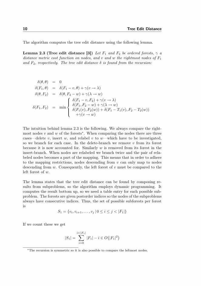
The algorithm computes the tree edit distance using the following lemma.
Lemma 2.3 (Tree edit distance [3]) Let F1 and F2 be ordered forests, γ adistance metric cost function on nodes, and v and w the rightmost nodes of F1
and F2, respectively. The tree edit distance δ is found from the recursion:
δ(θ, θ) = 0δ(F1, θ) = δ(F1 − v, θ) + γ(v → λ)δ(θ, F2) = δ(θ, F2 − w) + γ(λ→ w)
δ(F1, F2) = min
δ(F1 − v, F2) + γ(v → λ)δ(F1, F2 − w) + γ(λ→ w)δ(F1(v), F2(w)) + δ(F1 − T1(v), F2 − T2(w))
+γ(v → w)
The intuition behind lemma 2.3 is the following. We always compare the right-most nodes v and w of the forests∗. When comparing the nodes there are threecases—delete v, insert w, and relabel v to w—which have to be investigated,so we branch for each case. In the delete-branch we remove v from its forestbecause it is now accounted for. Similarly w is removed from its forest in theinsert-branch. When nodes are relabeled we branch twice and the pair of rela-beled nodes becomes a part of the mapping. This means that in order to adhereto the mapping restrictions, nodes descending from v can only map to nodesdescending from w. Consequently, the left forest of v must be compared to theleft forest of w.
The lemma states that the tree edit distance can be found by composing re-sults from subproblems, so the algorithm employs dynamic programming. Itcomputes the result bottom up, so we need a table entry for each possible sub-problem. The forests are given postorder indices so the nodes of the subproblemsalways have consecutive indices. Thus, the set of possible subforests per forestis
S1 = {vi, vi+1, . . . , vj | 0 ≤ i ≤ j < |F1|}
If we count these we get
|S1| =i<|F1|∑i=0
|F1| − i ∈ O(|F1|2
)∗The recursion is symmetric so it is also possible to compare the leftmost nodes.
2.2 Algorithms 11
subproblems. Since we require |F1|2|F2|2 subproblems to be computed we havenow established that a naive algorithm can compute the tree edit distance inO(|T1|2|T2|2
)† time and space.
We now show how the space bounds can be improved. We observe from therecursion that it is either the rightmost node of one of the forests that is removedor all but the rightmost tree. Therefore, it would suffice to have a |F1||F2|dynamic programming table if the solution to any subproblem consisting of twotrees was already known.
This is utilized by the algorithm as follows. We maintain a permanent tableof size |T1||T2| for all subproblems that consists of two trees. We solve eachsubproblem from the permanent table in the function Treedist. In Treedistwe create a temporary table of at most size |T1||T2| to hold the subproblemsthat are needed to solve the subproblem from the permanent table. If we needa subproblem to solve another subproblem that is not present in the temporarytable while in Treedist, it is because it consists of two trees, and the solutioncan thus be read from the permanent table. Since we maintain one table of size|T1||T2| and one of at most size |T1||T2|, the space bound has been improved toO(|T1||T2|
).
The time bound can also be improved. Occasionally, when in Treedist, wesolve a subproblem which consist of two trees. This happens for all pairs ofsubtrees where at least one tree is rooted on the path from the root of a treeto its leftmost leaf. Such a subproblem has already been solved in anotherinvocation of Treedist.
To take advantage of this, we define the notion of a keyroot. A keyroot is anode that has one or more siblings to the left. Then we only invoke Treediston subproblems from the permanent table where both trees have keyroots asroots. In Treedist we save the result of a subproblem in the permanent tableif it consists of two trees where at least one of them is not a rooted at a keyroot.Zhang and Shasha show that there is min
(leaves(T ), height(T )
)keyroots in a
tree T , so the running time of the algorithm is
O(|T1||T2| ·min
(leaves(T1), height(T1)
)·min
(leaves(T2), height(T2)
)The algorithm ZhangShasha and its subprocedure Treedist are given in thefollowing pseudocode.
†For simplicity we will state the time and space bounds as functions of input trees. Thepreceeding derivation uses the size of the forests because it has its starting point in therecursion. Subsequent tree edit distance algorithms do not accept forests as input.
12 Tree Edit Distance
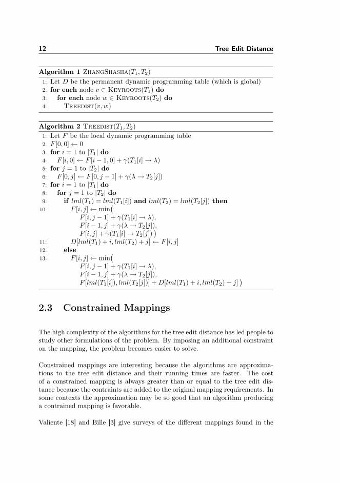
Algorithm 1 ZhangShasha(T1, T2)1: Let D be the permanent dynamic programming table (which is global)2: for each node v ∈ Keyroots(T1) do3: for each node w ∈ Keyroots(T2) do4: Treedist(v, w)
Algorithm 2 Treedist(T1, T2)1: Let F be the local dynamic programming table2: F [0, 0]← 03: for i = 1 to |T1| do4: F [i, 0]← F [i− 1, 0] + γ(T1[i]→ λ)5: for j = 1 to |T2| do6: F [0, j]← F [0, j − 1] + γ(λ→ T2[j])7: for i = 1 to |T1| do8: for j = 1 to |T2| do9: if lml(T1) = lml(T1[i]) and lml(T2) = lml(T2[j]) then
10: F [i, j]← min(
F [i, j − 1] + γ(T1[i]→ λ),F [i− 1, j] + γ(λ→ T2[j]),F [i, j] + γ(T1[i]→ T2[j])
)11: D[lml(T1) + i, lml(T2) + j]← F [i, j]12: else13: F [i, j]← min
(F [i, j − 1] + γ(T1[i]→ λ),F [i− 1, j] + γ(λ→ T2[j]),F [lml(T1[i]), lml(T2[j])] +D[lml(T1) + i, lml(T2) + j]
)
2.3 Constrained Mappings
The high complexity of the algorithms for the tree edit distance has led people tostudy other formulations of the problem. By imposing an additional constrainton the mapping, the problem becomes easier to solve.
Constrained mappings are interesting because the algorithms are approxima-tions to the tree edit distance and their running times are faster. The costof a constrained mapping is always greater than or equal to the tree edit dis-tance because the contraints are added to the original mapping requirements. Insome contexts the approximation may be so good that an algorithm producinga contrained mapping is favorable.
Valiente [18] and Bille [3] give surveys of the different mappings found in the
2.3 Constrained Mappings 13
litterature. In this section we will describe the top-down and isolated-subtreemappings.
2.3.1 Top-down
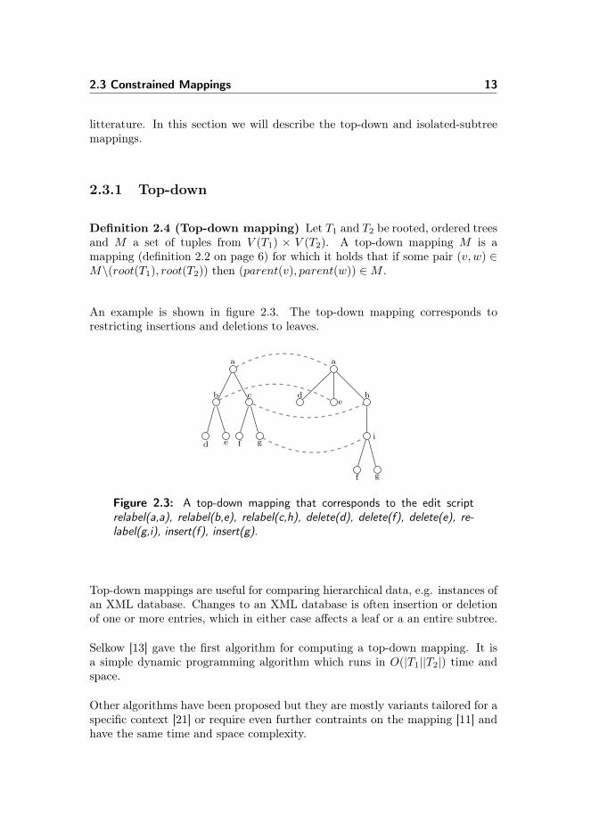
Definition 2.4 (Top-down mapping) Let T1 and T2 be rooted, ordered treesand M a set of tuples from V (T1) × V (T2). A top-down mapping M is amapping (definition 2.2 on page 6) for which it holds that if some pair (v, w) ∈M\(root(T1), root(T2)) then (parent(v), parent(w)) ∈M .
An example is shown in figure 2.3. The top-down mapping corresponds torestricting insertions and deletions to leaves.
a
b
d e
c
f g
a
de
h
i
f g
Figure 2.3: A top-down mapping that corresponds to the edit scriptrelabel(a,a), relabel(b,e), relabel(c,h), delete(d), delete(f), delete(e), re-label(g,i), insert(f), insert(g).
Top-down mappings are useful for comparing hierarchical data, e.g. instances ofan XML database. Changes to an XML database is often insertion or deletionof one or more entries, which in either case affects a leaf or a an entire subtree.
Selkow [13] gave the first algorithm for computing a top-down mapping. It isa simple dynamic programming algorithm which runs in O(|T1||T2|) time andspace.
Other algorithms have been proposed but they are mostly variants tailored for aspecific context [21] or require even further contraints on the mapping [11] andhave the same time and space complexity.

14 Tree Edit Distance
2.3.2 Isolated-subtree Mapping
Definition 2.5 (Isolated-subtree mapping) Let T1 and T2 be rooted, or-dered trees and M a set of tuples from V (T1) × V (T2). An isolated-subtreemappingM is a mapping (definition 2.2 on page 6) for which it holds that for anythree pairs (v1, w1), (v2, w2), (v3, w3) ∈M then nca(v1, v2) = nca(v1, v3) iff nca(w1, w2) =nca(w1, w3).
The intuition of this mapping is that subtrees must map to subtrees. In theexample shown in figure 2.4 we see that the pair (d, d) is not in the mappingM as it was in the non-contrained mapping because nca(e, d) 6= nca(e, f) in theleft tree whereas nca(e, d) = nca(e, f) in the right tree. In other words, e and dhave become part of two different subtrees in the right tree.
a
b
d e
c
f g
a
de
h
i
f g
Figure 2.4: An isolated-subtree mapping that corresponds to the editscript relabel(a,a), delete(b), delete(d), relabel(e,e), relabel(c,h), rela-bel(f,f), relabel(g,g), insert(d), insert(i).
For some applications of tree edit distance there may not be any differencebetween this and the original mapping. If we know that changes in the datais only relevant to the subtree they occur in, this mapping may even producemore useful results.
Zhang [23] presents a O(|T1||T2|) time and space algorithm. Because it is adynamic programming algorithm, the time complexity is valid for both best,average, and the worst case. However, it relies on a heavily modified versionof the recursion from lemma 2.3 on page 10 which makes it quite complex inpractice. Richter [12] presents an algorithm very similar to Zhangs but with adifferent O
(degree(|T1|) ·degree(|T2|) · |T1||T2|
)/O(degree(T1) ·height(T1) · |T2|
)time/space tradeoff. The worst case of this algorithm is of course when the treeshave a very high degree.
2.4 Approximate Tree Pattern Matching 15
2.4 Approximate Tree Pattern Matching
A tree edit distance algorithm based on lemma 2.3 on page 10 can be modifiedto be used for approximate tree pattern matching. In tree pattern matching wedenote the data tree TD and the pattern tree TP .
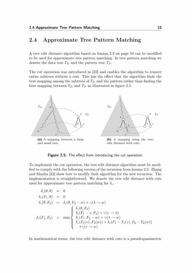
The cut operation was introduced in [22] and enables the algorithm to removeentire subtrees without a cost. This has the effect that the algorithm finds thebest mapping among the subtrees of TD and the pattern rather than finding thebest mapping between TD and TP as illustrated in figure 2.5.
b
a
c
a
bc
TP
TD
(a) A mapping between a largeand small tree.
b
a
c
a
bc
d
TP
TD
(b) A mapping using the treeedit distance with cuts.
Figure 2.5: The effect from introducing the cut operation.
To implement the cut operation, the tree edit distance algorithm must be modi-fied to comply with the following version of the recursion from lemma 2.3. Zhangand Shasha [22] show how to modify their algorithm for the new recursion. Theimplementation is straightforward. We denote the tree edit distance with cutsused for approximate tree pattern matching for δc.
δc(θ, θ) = 0δc(F1, θ) = 0δc(θ, F2) = δc(θ, F2 − w) + γ(λ→ w)
δc(F1, F2) = min
δc(θ, F2)δc(F1 − v, F2) + γ(v → λ)δc(F1, F2 − w) + γ(λ→ w)δc(F1(v), F2(w)) + δc(F1 − T1(v), F2 − T2(w))
+γ(v → w)
In mathematical terms, the tree edit distance with cuts is a pseudoquasimetric
16 Tree Edit Distance
which means δc(T1, T2) can be 0 when T1 6= T2 and δc(T1, T2) can differ fromδc(T2, T1) [27]. The proviso from this is that we consistently must give the datatree as first argument to the algorithm.
The tree edit distance with cuts reflects changes to the subtree mapped to thepattern as well as the depth of the mapping. Consequently, the deeper themapping is the less errors we allow within the actual pattern. To deal with this,Zhang, Shasha and Wang [19] present an algorithm which takes variable lengthdon’t cares (abbreviated VLDC and also commonly referred to as wildcards) inthe pattern into account. It resembles Zhang and Shasha’s algorithm and hasthe same time and space complexity.

Chapter 3
Web Scraping usingApproximate Tree Pattern
Matching
In this chapter it is shown how to apply approximate tree pattern matching toweb scraping. We then discuss the algorithms from the previous chapter in rela-tion to web scraping and give an overview of related work from the litterature.
3.1 Basic Procedure
The layout of a web site, i.e. the presentation of data, is described using Hyper-text Markup Language (HTML). An HTML document basically consists of fourtype of elements: document structure, block, inline, and interactive elements.There is a Document Type Definition (DTD) for each version of HTML whichdescribes how the elements are allowed to be nested∗. It is structured as a gram-mar in extended Backus Naur form. There is a strict and a transitional versionof the DTD for backward compatability. The most common abstract model for∗The DTD also describes optional and mandatory attributes for the elements, but this is
irrelevant to our use.

18 Web Scraping using Approximate Tree Pattern Matching
HTML documents are trees. An example of a HTML document modelled as atree is shown in figure 3.1.
� �1 <html>2 <head>3 <title>Example </title>4 </head>5 <body>6 <h1>Headline </h1>7 <table>8 <tr>9 <td>a</td>
10 <td>b</td>11 </tr>12 <tr>13 <td>c</td>14 <td>d</td>15 </tr>16 </table >17 </body>18 </html>� �
html
head
title
Example
body
h1
Headline
table
tr
td
a
td
b
tr
td
c
td
d
Figure 3.1: A HTML document and its tree model.
Changes in the HTML document affects its tree model so a tree edit distancealgorithm can be used to identify structural changes. Furthermore, approximatetree pattern matching can be used to find matchings of a pattern in the HTMLtree. For this purpose, the pattern is the tree model of a subset of a HTMLdocument.
Utilizing the above for web scraping is straightforward. First we have to gener-ate† or manually define a pattern. The pattern must contain the target nodes,i.e. the nodes from which we want to extract data. Typically, the pattern couldbe defined by extracting the structure of the part of the web site we wish toscrape the first time it is visited. Then we parse the HTML and build a datatree. Running the algorithm with the data and pattern trees gives a mapping.We are now able to search the mapping for the target nodes and extract thedesired data.
†Automatic generation of a pattern is more commonly referred to as learning a pattern.Given a set of pages from a web site, a learning algorithm can detect the similarities andcreate a pattern. Learning is beyond the scope of this project.

3.2 Pattern Design 19
3.2 Pattern Design
When using approximate tree pattern matching, the pattern plays an importantrole to the quality of the result produced by an algorithm. We now discuss howto design patterns for the purpose of web scraping.
We will use Reddit‡ (www.reddit.com) as the running example in our discussion.Consider the screenshot of the front page of Reddit in figure 3.2. It shows asmall topic toolbar followed by the Reddit logo and the highest rated entries.Notice that the entry encapsulated in a box with a light blue background is asponsored entry, as opposed to the other entries, which are submitted by Redditusers.
Figure 3.2: A selection of entries from the frontpage of Reddit (2011-06-25).
Say we want to extract the title, URL to the image, and time of submission ofthe first entry. Then it suffices to use the substructure (shown in figure 3.3 onthe following page) of the entries as pattern. This pattern will actually matchthe first entry that has a picture.
We may not be interested in extracting the sponsored entry. Conveniently, thesponsored entry and the user submitted entries reside in separate <div> con-tainers. So to exclusively target the user submitted entries we have to modifythe pattern to include an anchor that is long enough for the algorithm to dis-tinguish between the sponsored entry and the user submitted entries. In thiscase the pattern is given an anchor consisting of two div elements. The second
‡Reddit is a user driven community where users can submit links to content of the Internetor self-authored texts. The main feature of the site is the voting system which bring aboutthat the best submissions are on the top of the lists.

20 Web Scraping using Approximate Tree Pattern Matching
� �1 <div><!-- Entry -->2 <a><img /><!-- Image --></a>3 <div>4 <p>5 <a><!-- Title --></a>6 </p>7 <p>8 <time><!-- Time --></time>9 </p>
10 </div>11 </div>� �
div
a
img
div
p
a
p
time
Figure 3.3: A pattern for a Reddit entry and its tree model.
element is given an id attribute to distinguish the container for the sponsoredentries from the container for user entries. It is shown in figure 3.4.
� �1 <div>2 <div id="siteTable">3 <div><!-- User entry -->4 <a><img /><!-- Image --></a>5 <div>6 <p>7 <a><!-- Title --></a>8 </p>9 <p>
10 <a><!-- Time --></a>11 </p>12 </div>13 </div>14 </div>15 </div>� �
div
div
div
a
img
div
p
a
p
time
Figure 3.4: A pattern with an anchor for a Reddit entry and its treemodel.
The main disadvantage of adding an anchor is that the pattern becomes largerwhich affects the execution time of the algorithm. Using attributes in the patternalso faces the risk that the value may be changed by the web designer. If theid is changed in this example, the pattern will match the sponsored entry justas well.
3.3 Choosing an Algorithm 21
3.3 Choosing an Algorithm
Having decided on using approximate tree pattern matching for web scraping,there is still a selection of algorithms to choose from.
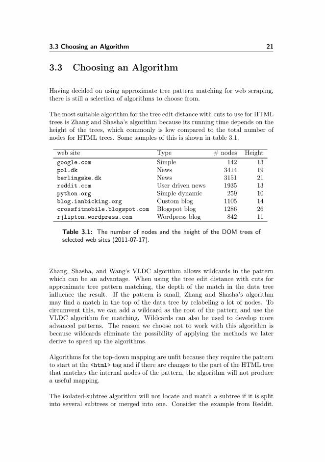
The most suitable algorithm for the tree edit distance with cuts to use for HTMLtrees is Zhang and Shasha’s algorithm because its running time depends on theheight of the trees, which commonly is low compared to the total number ofnodes for HTML trees. Some samples of this is shown in table 3.1.
web site Type # nodes Heightgoogle.com Simple 142 13pol.dk News 3414 19berlingske.dk News 3151 21reddit.com User driven news 1935 13python.org Simple dynamic 259 10blog.ianbicking.org Custom blog 1105 14crossfitmobile.blogspot.com Blogspot blog 1286 26rjlipton.wordpress.com Wordpress blog 842 11
Table 3.1: The number of nodes and the height of the DOM trees ofselected web sites (2011-07-17).
Zhang, Shasha, and Wang’s VLDC algorithm allows wildcards in the patternwhich can be an advantage. When using the tree edit distance with cuts forapproximate tree pattern matching, the depth of the match in the data treeinfluence the result. If the pattern is small, Zhang and Shasha’s algorithmmay find a match in the top of the data tree by relabeling a lot of nodes. Tocircumvent this, we can add a wildcard as the root of the pattern and use theVLDC algorithm for matching. Wildcards can also be used to develop moreadvanced patterns. The reason we choose not to work with this algorithm isbecause wildcards eliminate the possibility of applying the methods we laterderive to speed up the algorithms.
Algorithms for the top-down mapping are unfit because they require the patternto start at the <html> tag and if there are changes to the part of the HTML treethat matches the internal nodes of the pattern, the algorithm will not producea useful mapping.
The isolated-subtree algorithm will not locate and match a subtree if it is splitinto several subtrees or merged into one. Consider the example from Reddit.
22 Web Scraping using Approximate Tree Pattern Matching
Assume that a new visualization of the entries, where the second div is super-flous, is introduced. This corresponds to merging the two subtrees of the rootof the pattern into one. As shown in figure 3.5 on the next page, the img tagwill not be located when using the isolated-subtree mapping.
3.4 Extracting Several Matches
Until now we have assumed that we only want to extract the optimal match.However, it is common that we want to extract several matches. Continuingwith Reddit as example we may want to extract all entries from the front page.In this section we discuss how to achieve this using approximate tree patternmatching.
If we know how many entries we want to extract, one approach is to create apattern that matches the required number of entries. This also applies if wewant to extract the nth entry. Then we create a pattern matching the first nentries and discard the results for the first n− 1 entries. The drawback of thisapproach is that the pattern quickly becomes big and slows down the algorithm.Also, when creating a pattern for n entries we are not guaranteed that it willmatch the first n entries. It will match some n entries.
The above mentioned method is not applicable if we want to extract all entrieswithout knowing the exact number of entries. An alternative approach is tocreate a pattern matching one entry. After matching the pattern we remove thenodes in the mapping from the data tree. This is repeated until the cost of themapping exceeds some predefined threshold.
The main disadvantage of this approach is that the algorithm has to be invokedseveral times. Furthermore, if the goal is to extract the first n entries we cannotguarantee that the pattern matches the first n entries in n invocations of thealgorithm.
3.5 Related Work
The litterature on information extraction from web sites is vast. However, thefocus is mostly on learning patterns and information extraction§ from data. We
§Information extraction is extraction of meaningful content from web sites without explic-itly specifying where the information reside.

3.5 Related Work 23
div
a
img
div
p
a
p
time
(a) A Reddit entrybefore the change.Subtree is used aspattern.
div
a
img
p
a
p
time
(b) A Reddit entry afterthe change.
div
a
img
p
a
p
time
div
a
img
div
p
a
p
time
(c) The optimal mapping as produced by e.g. Zhang andShasha’s algorithm.
div
a
img
p
a
p
time
div
a
img
div
p
a
p
time
(d) The isolated-subtree mapping.
Figure 3.5: Example of the difference in outcome from using an originalmapping and an isolated-subtree mapping.

24 Web Scraping using Approximate Tree Pattern Matching
will review the known results from using approximate tree pattern matching inthis context.
Xu and Dyreson [20] present an implementation of XPath which finds approxi-mate matches. The algorithm is based on the Apache Xalan XPath evaluationalgorithm, but the criteria for the algorithm is that the result must be within kedits of the HTML tree model. The algorithm runs in O
(k · |TP ||TD| log |TD|
)time, but bear in mind that this is for evaluating a path. To simulate match-ing a tree pattern we need several paths [28] and the running time becomesO(k · |TP |2|TD| log |TD|
)(worst case), which is worse than Zhang and Shasha’s
algorithm. Also, it matches each path of the pattern separately so it does notobey the mapping criterias we know from the tree edit distance.
Reis et al. [11] presents an algorithm for extraction of information from setsof web sites. Given a set of web sites they generate a pattern with wildcards.Using the pattern their algorithm computes a top-down mapping, but unlikeother algorithms for the top-down mapping it does not compute irrelevant sub-problems based on a max distance k given as input. The worst case runningtime is O
(|T1||T2|
)but due to the deselection of irrelevant subproblems, the
average case is a lot faster. Their algorithm works well because their patterngeneration outputs a pattern which is sufficiently restricted to be used with atop-down algorithm.
Based on the claim that information extraction or web scraping using tree pat-tern matching is flawed, Kim et al. [8] suggests a cost function that takes therendered size of tags into account when comparing them. They use the costfunction with an algorithm for the top-down mapping.
3.6 Summary
The most suited algorithm for web scraping is Zhang and Shasha’s algorithm,but we anticipate that it will be slow on large webpages. The Reddit exampleshows that there is a case where Zhang’s algorithm for the isolated-subtreemapping fails to locate the targeted data.
The speed issue is not adressed directly in the litterature because sub-optimalalgorithms are used in return for pattern constraints. The remainder of this the-sis will focus on speeding up the algorithm aiming at attaining a more versatilesolution than found in the litterature.
Chapter 4
Lower Bounds for Tree EditDistance with Cuts
In this chapter we describe six methods for approximating the tree edit distancewith cuts. The methods are all lower bounds for the tree edit distance with cuts.The methods are derived from attempts to approximate the tree edit distance(without cuts) in the litterature.
The methods are all based on the assumption that a unit cost function is used,and we will use D to denote the approximations of the tree edit distance withcuts.
4.1 Tree Size and Height
When a unit cost function is used, the edit distance between two trees is boundedfrom below by the difference in the size of the trees. Consider two trees T1 andT2 where |T1| > |T2|. To change T1 to T2 at least |T1| − |T2| nodes must beremoved from T1. Similarly, if T2 is a larger tree than T1, at least |T2| − |T1|nodes must be inserted in T1 to change it to T2.
When using the tree edit distance for approximate tree pattern matching we

26 Lower Bounds for Tree Edit Distance with Cuts
include the cut operation, so some nodes may be deleted from T1 without af-fecting the cost. Therefore, it is impossible to determine, based on the size ofthe trees, if T2 can be obtained by using only cut on T1. As a result, the lowerbound Dsize is:
Dsize(T1, T2) = max(0, |T2| − |T1|
)(4.1)
Assuming the nodes of a tree T have postorder indices, then the nodes of anysubtree T (v) is a consecutive sequence of indices starting from the index of theleftmost leaf of the subtree to the index of the root of the tree. So the size ofa tree can be found from |T (v)| = v − lml(v), which can be found in constanttime after a O(|T |)-preprocessing of the tree.
Alternatively, the height of the trees can be used as a lower bound as shownbelow. This can produce a tighter lower bound for trees that may be very similarin terms of size but otherwise look very different.
Dheight(T1, T2) = max(0, height(T2)− height(T1)
)(4.2)
4.2 Q-gram Distance
The q-gram is a concept from string matching theory. A q-gram is a substringof length q. The q-gram distance between two strings x and y is defined asfollows. Let Σ be the alphabet of the strings and Σq all strings of length q inΣ. Let G(x)[v] denote the number of occurrences of the string v in the stringx. The q-gram distance for strings dq is obtained from the following equation[17].
dq(x, y) =∑v∈Σq
∣∣G(x)[v]−G(y)[v]∣∣ (4.3)
If d(x, y) is the optimal string edit distance between x and y, the q-gram distancecan be 0 ≤ dq(x, y) ≤ d(x, y) ·q, given that unit cost is used for all operations onthe strings. So the q-gram distance may exceed the optimal string edit distance.To use the q-gram distance as a lower bound for the string edit distance, wecan select a disjoint set of q-grams from x. Then one character in the stringcan only affect one q-gram and thereby only account for one error in the q-gramdistance. As a result 0 ≤ dq(x, y) ≤ |x|q ≤ e.
We generalize the q-gram distance to trees by using subpaths of a tree as q-grams. In one tree we select all subpaths of size 1 to q. In the other tree weensure that the tree q-gram distance is a lower bound for the tree edit distanceby selecting a disjoint set of q-grams (when disjoint we call them q-samples) ofsize at most q.
4.2 Q-gram Distance 27
We select q-grams of different sizes to be able to include any node in at least oneq-gram and thereby make the lower bound on the tree edit distance tighter. Ifq > 1 and the tree has more than 2q nodes, there will be more than one way toselect a disjoint set of q-grams. Therefore, the algorithm which selects q-gramsmay influence on the q-gram distance for trees.
The q-gram distance can be extended to allow for the cut operation. A q-gramthat appears in T1 and not T2 may not be accounted as an error, whereas itmay if it appears in T2 and not in T1. So the tree q-gram distance with cuts is
Dq(T1, T2) =∑Q∈T2
max(0, G(T2)[Q]−G(T1)[Q]
)(4.4)
In practice, we only have to iterate the q-grams in T2 to make the above com-putation. Since the q-grams of T2 are disjoint, there can be at most |T2| ofthem. Thus, the tree q-gram distance with cuts can be computed in O(|T2|)time (assuming the q-grams have been computed in a pre-processing step).
Having defined the q-gram distance with cuts, we now show that it is a lowerbound for the tree edit distance with cuts if the q-grams in T2 are disjoint.
Lemma 4.1 Let Dq(T1, T2) be the tree q-gram distance with cuts for two treesT1 and T2, and let the q-grams in T2 be disjoint. Then
Dq(T1, T2) ≤ δc(T1, T2) (4.5)
Proof. If δc(T1, T2) > 0 then there is at least one node v in T2 which is not inT1. Let v be part of a q-gram in T2 which is not in T1. The only free operationthat makes structural changes to T1 is cut. If we remove a leaf we reduce theset of q-grams in T1 and then the q-gram with v is still not in T1. Therefore, weneed k operations, where 1 ≤ k ≤ q, to create the q-gram of T2 in T1. If c is thenumber of q-grams in T2 which are not in T1 then we have c ≤ δc(T1, T2) ≤ c · q,and since each q-gram can account for only one error we have Dq(T1, T2) = c.(4.5) clearly follows from this. If δc(T1, T2) = 0 then T2 is a subtree in T1 andany q-gram in T2 is also in T1. �
The chosen value of q will affect the outcome of (4.4). A small value for qmay produce a tight bound for dissimilar trees. If the trees do not have alot in common, we want as many q-grams as possible in order to capture thedifferences. For similar trees, a larger value for q may produce a tight bound.Larger q-grams contain more information about the structure of the tree. If thetrees are similar, and the q-grams are small, we risk missing an error.

28 Lower Bounds for Tree Edit Distance with Cuts
We may also select overlapping q-grams from T2 if we bound the number ofq-grams a node is allowed to be part of and subsequently divide the distanceby the bound. However, there may be q-grams not present in T1 due to nodeswhich are only in one q-gram in T2, and we anticipate that the extra q-gramsin T2 do not make up for this.
Algorithms for computing q-grams and q-samples for a tree are given in ap-pendix B.1 on page 83 and appendix B.2.
4.3 PQ-gram Distance
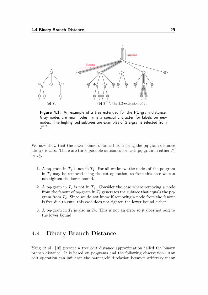
Augsten et al. [2] present another generalization of the q-gram distance whichis based on pq-grams. A pq-gram is a subtree which consists of a path of lengthp from its root to an internal node v. This is the anchor. The node v has qchildren. This is the fanout. When referring to a specific set of pq-grams wherethe parameters are set to for instance p = 2 and q = 3 we call them 2,3-grams.We describe their method and show why it can not be adapted to the tree editdistance with cuts.
The generalization of q-grams to subpaths only captures information about theparent/child relationship between nodes. The advantage of the pq-gram is thatit is possible to capture more structural information than with q-grams, becauseeach pq-gram holds information of the relation between children of a node. Toenable us to select as many pq-grams as possible a tree is extended such that
• the root has p− 1 ancestors,
• every internal node has an additional q − 1 children before its first child,
• every internal node has an additional q − 1 children after its last child,
• every leaf has q children
The resulting tree is called the T p,q-extended tree of T . An example of a tree,its extended tree, and a disjoint set of pq-grams is seen in figure 4.1 on the nextpage.
The pq-gram distance is computed the same way as the q-gram distance forstrings, and Augsten et al. prove that it is a lower bound for the fanout treeedit distance, which is obtained from using a cost function that depends on thedegree of the node to operate on.
4.4 Binary Branch Distance 29
a
b
d e
b c
f
(a) T .
ε
a
ε b
εd
ε ε
e
ε ε
ε
b
ε ε
c
εf
ε ε
ε
ε
anchor
fanout
(b) T 2,2, the 2,2-extension of T .
Figure 4.1: An example of a tree extended for the PQ-gram distance.Gray nodes are new nodes. ε is a special character for labels on newnodes. The highlighted subtrees are examples of 2,2-grams selected fromT 2,2.
We now show that the lower bound obtained from using the pq-gram distancealways is zero. There are three possible outcomes for each pq-gram in either T1
or T2.
1. A pq-gram in T1 is not in T2. For all we know, the nodes of the pq-gramin T1 may be removed using the cut operation, so from this case we cannot tighten the lower bound.
2. A pq-gram in T2 is not in T1. Consider the case where removing a nodefrom the fanout of pq-gram in T1 generates the subtree that equals the pq-gram from T2. Since we do not know if removing a node from the fanoutis free due to cuts, this case does not tighten the lower bound either.
3. A pq-gram in T1 is also in T2. This is not an error so it does not add tothe lower bound.
4.4 Binary Branch Distance
Yang et al. [16] present a tree edit distance approximation called the binarybranch distance. It is based on pq-grams and the following observation. Anyedit operation can influence the parent/child relation between arbitrary many
30 Lower Bounds for Tree Edit Distance with Cuts
nodes whereas it can only influence exactly two sibling relations. By convertingthe trees to their binary tree representations and selecting all possible 1,2-grams,the authors show that the pq-gram distance (of the transformed problem) is atmost 4 times the tree edit distance. The result is thus a lower bound which isfound without having to select a disjoint set of pq-grams from one of the trees.We describe their method and show why it can not be extended to include thecut operation.
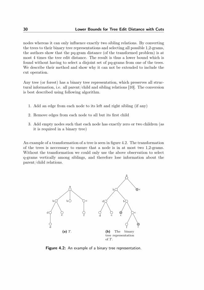
Any tree (or forest) has a binary tree representation, which preserves all struc-tural information, i.e. all parent/child and sibling relations [10]. The conversionis best described using following algorithm.
1. Add an edge from each node to its left and right sibling (if any)
2. Remove edges from each node to all but its first child
3. Add empty nodes such that each node has exactly zero or two children (asit is required in a binary tree)
An example of a transformation of a tree is seen in figure 4.2. The transformationof the trees is neccessary to ensure that a node is in at most two 1,2-grams.Without the transformation we could only use the above observation to selectq-grams vertically among siblings, and therefore lose information about theparent/child relations.
a
b
d
d
e
b c
f
(a) T .
a
b
d
d e
b
εc
f ε
ε
(b) The binarytree representationof T .
Figure 4.2: An example of a binary tree representation.
4.4 Binary Branch Distance 31
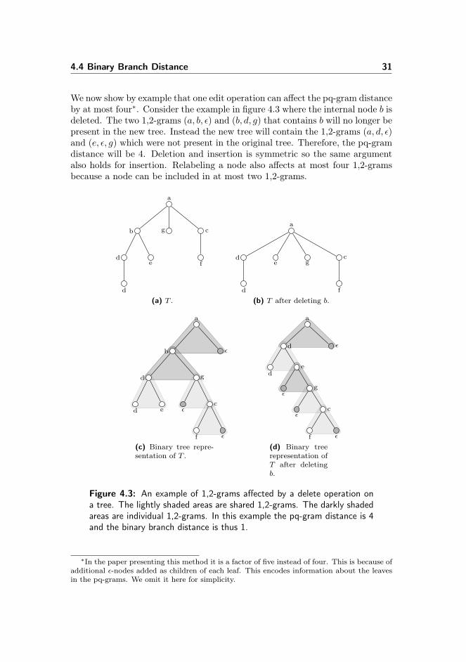
We now show by example that one edit operation can affect the pq-gram distanceby at most four∗. Consider the example in figure 4.3 where the internal node b isdeleted. The two 1,2-grams (a, b, ε) and (b, d, g) that contains b will no longer bepresent in the new tree. Instead the new tree will contain the 1,2-grams (a, d, ε)and (e, ε, g) which were not present in the original tree. Therefore, the pq-gramdistance will be 4. Deletion and insertion is symmetric so the same argumentalso holds for insertion. Relabeling a node also affects at most four 1,2-gramsbecause a node can be included in at most two 1,2-grams.
a
b
d
d
e
g c
f
(a) T .
a
d
d
e gc
f
(b) T after deleting b.
a
b
d
d e
g
εc
f ε
ε
(c) Binary tree repre-sentation of T .
a
d
de
εg
εc
f ε
ε
(d) Binary treerepresentation ofT after deletingb.
Figure 4.3: An example of 1,2-grams affected by a delete operation ona tree. The lightly shaded areas are shared 1,2-grams. The darkly shadedareas are individual 1,2-grams. In this example the pq-gram distance is 4and the binary branch distance is thus 1.
∗In the paper presenting this method it is a factor of five instead of four. This is because ofadditional ε-nodes added as children of each leaf. This encodes information about the leavesin the pq-grams. We omit it here for simplicity.

32 Lower Bounds for Tree Edit Distance with Cuts
The binary branch distance is potentially a tighter lower bound of the tree editdistance than the q-gram and pq-gram distance because it allows us to selectoverlapping pq-grams from both trees and because it captures sibling relations.However, since the distance must be divided by 4 we need to select 4 times asmany pq-grams as we would select disjoint q-grams.
However, the binary branch distance can not be used to produce a lower boundfor the tree edit distance with cuts. This is evident from the three possibleoutcomes for a 1,2-gram in either T1 or T2.
1. A pq-gram in T1 is not in T2. The nodes of the pq-gram may be part of asubtree that can be cut away, so this can not be used to tighten the lowerbound.
2. A pq-gram in T2 is not in T1. Consider the tree T of figure 4.3 on thepreceding page. Assume that the node a has a child v between g andc. Then the 1,2-grams (g, ε, c) and (c, f, ε) would not be present in T2.However, if v is cut away, which is free, then the two pq-grams becomespresent in T1. Therefore, a pq-gram in T2 and not T1 can not count as anerror.
3. A pq-gram in T1 is also in T2. This is not an error so it does not add tothe lower bound.
4.5 Euler String Distance
Hierarchical structured data is commonly represented as trees, but may also berepresented as a parenthesized string called the Euler string. The parenthesesare used to maintain parent/child relationships. Consider for instance the tree infigure 4.4 on the next page whose Euler string representation is a(b(de)cb(b)).The Euler string is computed by doing a postorder traversal of the nodes. Itcan be computed in O(|T |) time and the tree can be restored again in O(|T |)time. However, serialization of tree data has the disadvantage that parent/childrelations no longer can be determined in constant time.
Another variant of the Euler string omits parentheses and uses a special invertedcharacter when backtracking from a node. An example is shown in figure 4.4on the facing page. The special characters must not be a part of the set ofall possible labels. This variant is more suited for comparison of the stringsbecause the number of extra characters, i.e. parentheses, is independent of thetree structure. We will use this variant and we denote the Euler string of a treeT for s(T ).

4.5 Euler String Distance 33
a
b
d e
c b
b
T
s(T ) = bddeebccbbbb
Figure 4.4: A tree and its Euler string.
The string edit distance of two Euler strings can be used as a lower bound forthe tree edit distance based on the following observation by Akutsu [1]. Anyoperation on a tree T affects at most two characters in s(T ), so we have thefollowing theorem.
Theorem 4.2 ([1]) Let T1 and T2 be ordered, rooted trees and let s(T ) denotethe Euler string of a tree T . Let d(x, y) denote the string edit distance of twostrings x and y and δ(T1, T2) the tree edit distance of the trees. Then we have
12d(s(T1), s(T2)
)≤ δ(T1, T2) (4.6)
For two strings of length m and n, computing the string edit distance can bedone in O(mn) time [5]. Since |s(T )| = O(T ) this method can compute anapproximation of the tree edit distance in O(|T1||T2|) time.
We will now discuss approaches to convert this method to give lower bounds forthe tree edit distance with cuts. We will discuss
• making all delete operations free in the string edit distance algorithm,
• postprocessing the result from the string edit distance algorithm,
• and modifying the string edit distance algorithm to handle cuts.
Making delete operations free for the string edit distance algorithm is the onlyeffective way of adapting this method to act as a lower bound for the tree editdistance with cuts. We start by showing that for any mapping obtained usingan algorithm for the tree edit distance with cuts, there is a mapping, producedby a regular tree edit distance algorithm, with the same cost or cheaper if usinga cost function where deletes are free.
34 Lower Bounds for Tree Edit Distance with Cuts
Lemma 4.3 Let T1 and T2 be ordered, rooted trees. Let δ(T1, T2) be the treeedit distance between T1 and T2 using a cost function γ where deletes are alwaysfree, i.e. γ(v → λ) = 0, ∀v ∈ V (T1). Let δc(T1, T2) be the tree edit distance withcuts. We then have
δ(T1, T2) ≤ δc(T1, T2) (4.7)
Proof. Assume that δ(T1, T2) > δc(T1, T2) for some two trees T1 and T2. Thenthere is an edit script E for δc(T1, T2) consisting of a inserts, b deletes, c relabels,and d cuts. Their accumulated cost is ca, cb, cc, and cd, respectively. The costof E is ca + cb + cc because cd = 0. If cuts are not available we would haveto replace cuts by deletes, so the cost of an edit script that produce the samemapping as E would be ca + cb + cc + cd. If deletes are free it is ca + cc. Fromour assumption we have that ca + cc > ca + cb + cc, which is a contradictionbecause costs are non-negative, cf. the cost function is a distance metric. �
We now establish that the string edit distance, where the delete operation iswithout a cost, of the Euler strings of two trees is a lower bound for the treeedit distance with cuts.
Lemma 4.4 Let d(x, y) be the string edit distance and δc(T1, T2) the tree editdistance with cuts. If we use a cost function for the string edit distance wheredelete operations are free then half the string edit distance is a lower bound ofthe tree edit distance with cuts, i.e.
12d(s(T1), s(T2)
)≤ δc(T1, T2) (4.8)
Proof. Since theorem 4.2 on the previous page holds for cost functions thatqualify as distance metrics, and the cost function where delete operations arefree is a distance metric, we can combine theorem 4.2 and lemma 4.3 to obtainthis lemma.
Thus, the tree Euler string edit distance De is
De(T1, T2) =12d(s(T1), s(T2)
)(4.9)
The remainder of this section will discuss why the two other approaches will notproduce a lower bound as required.
We would like to be able to correct for deletes in a postprocessing phase. Hereis an approach. Once a string edit distance has been computed, the sequence of
4.6 Summary 35
edit operations can be extracted using backtracking in the dynamic program-ming table. From the sequence of operations it is possible to compute a mappingbetween characters of the two strings. Assume the data string is split into a setof substrings by the characters in the mapping. For each of these substrings welook for a pair of a character and its inverted character, e.g. aa. This corre-sponds to a leaf and can be removed without a cost. This is repeated for eachsubstring until no more such pairs exist. The number of characters removedis subtracted from the string edit distance and the result is a lower bound forthe tree edit distance with cuts. Unfortunately, we can not guarantee that theresulting mapping is equal to the mapping an algorithm for the tree edit dis-tance with cuts would produce. This means that there may be fewer pairs ofcharacters to remove in the postprocessing phase, and therefore this approachcan not be used to compute a lower bound.
Modifying the string edit distance algorithm to handle cuts is not possible either.As mentioned earlier, information about the parent/child relations is lost whentree data is serialized. An algorithm will consider one character of the datastring at a time. To determine if we can cut away a character, the algorithmmust read at least one other character, which it will have to scan through thestring to find.
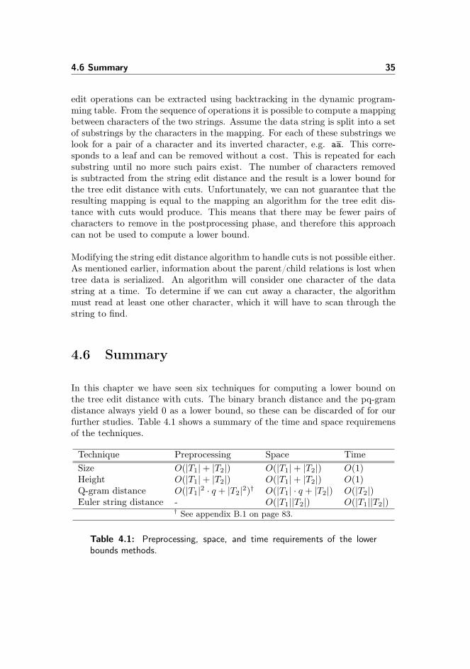
4.6 Summary
In this chapter we have seen six techniques for computing a lower bound onthe tree edit distance with cuts. The binary branch distance and the pq-gramdistance always yield 0 as a lower bound, so these can be discarded of for ourfurther studies. Table 4.1 shows a summary of the time and space requiremensof the techniques.
Technique Preprocessing Space TimeSize O(|T1|+ |T2|) O(|T1|+ |T2|) O(1)Height O(|T1|+ |T2|) O(|T1|+ |T2|) O(1)Q-gram distance O(|T1|2 · q + |T2|2)† O(|T1| · q + |T2|) O(|T2|)Euler string distance - O(|T1||T2|) O(|T1||T2|)
† See appendix B.1 on page 83.
Table 4.1: Preprocessing, space, and time requirements of the lowerbounds methods.

36 Lower Bounds for Tree Edit Distance with Cuts

Chapter 5
Data Tree Pruning andHeuristics
5.1 Adapting the Fast Unit Cost Algorithm toCuts
In [14] Shasha and Zhang present a tree edit distance algorithm which is fastfor similar trees, i.e. when the tree edit distance is small. It is fast because itassumes that a unit cost function is used, and based on that, some subproblemscan be ruled out while the algorithm still computes an optimal solution. In thissection we adapt the algorithm to cuts.
Not as many subproblems can be ruled out after the adaption. However, thealgorithm serves as inspiration to our pruning approach. Pruning of the datatree means reducing its size prior to running the actual algorithm. The dif-ference between pruning and ruling out subproblems at runtime is subtle butnotable. Pruning a branch of the data tree corresponds to ruling out all sub-problems containing any nodes in the subtree, so ruling out subproblems atruntime causes fewer subproblems to be computed. Instead, pruning offers twoother advantages. We can apply more elaborate methods to decide if a subtreeis relevant because we do not have to do it at runtime. And, as we shall see, wecan use keyroots when the tree is pruned prior to running the algorithm, which
38 Data Tree Pruning and Heuristics
is not possible when ruling out subproblems at runtime.
5.1.1 Algorithm Description
The fast unit cost algorithm by Shasha and Zhang is based on the following twoobservations.
1. The tree edit distance between two trees is at least the difference in thesize of the trees.
2. If the mapping between two subtrees T1(v) and T2(w) is part of an optimalsolution, then the mapping between the forests to the left of the subtreesis also a part of the optimal solution∗.
The observations are combined to rule out subproblems in the permanent dy-namic programming table as follows. The algorithm is given a threshold k asinput. A subproblem in the permanent table is ruled out if the difference in thesize of the subtrees plus the difference in the size of their left subforests exceedsthe threshold k. This is formalized in the following lemma.
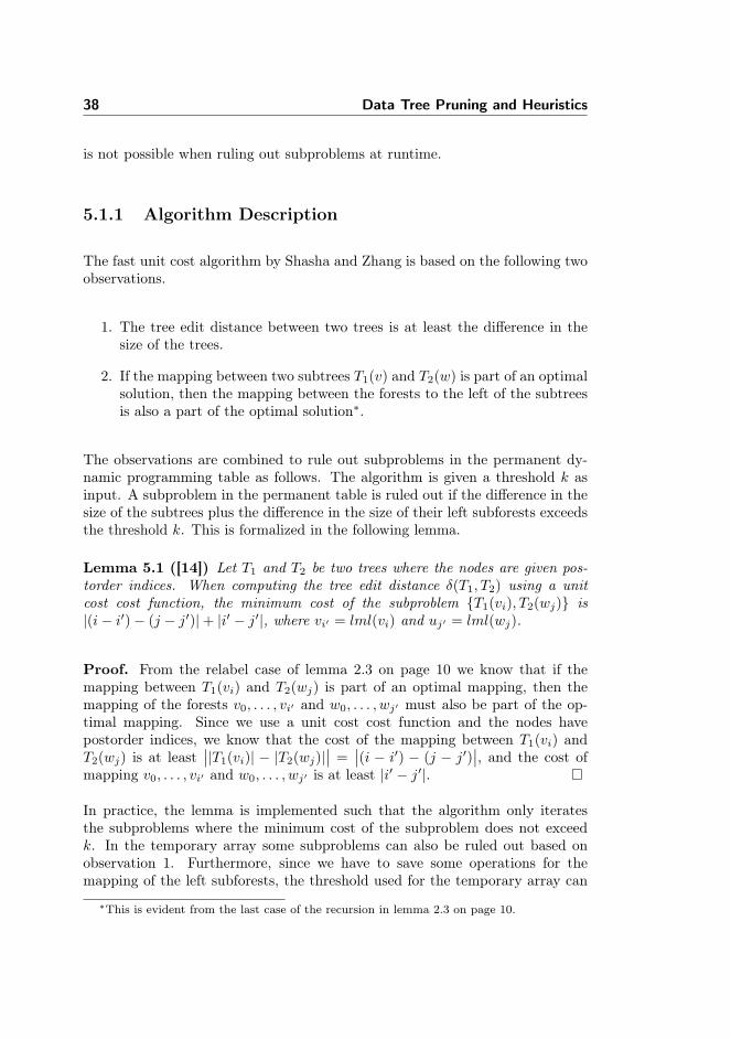
Lemma 5.1 ([14]) Let T1 and T2 be two trees where the nodes are given pos-torder indices. When computing the tree edit distance δ(T1, T2) using a unitcost cost function, the minimum cost of the subproblem {T1(vi), T2(wj)} is|(i− i′)− (j − j′)|+ |i′ − j′|, where vi′ = lml(vi) and uj′ = lml(wj).
Proof. From the relabel case of lemma 2.3 on page 10 we know that if themapping between T1(vi) and T2(wj) is part of an optimal mapping, then themapping of the forests v0, . . . , vi′ and w0, . . . , wj′ must also be part of the op-timal mapping. Since we use a unit cost cost function and the nodes havepostorder indices, we know that the cost of the mapping between T1(vi) andT2(wj) is at least
∣∣|T1(vi)| − |T2(wj)|∣∣ =
∣∣(i − i′) − (j − j′)∣∣, and the cost of
mapping v0, . . . , vi′ and w0, . . . , wj′ is at least |i′ − j′|. �
In practice, the lemma is implemented such that the algorithm only iteratesthe subproblems where the minimum cost of the subproblem does not exceedk. In the temporary array some subproblems can also be ruled out based onobservation 1. Furthermore, since we have to save some operations for themapping of the left subforests, the threshold used for the temporary array can
∗This is evident from the last case of the recursion in lemma 2.3 on page 10.

5.1 Adapting the Fast Unit Cost Algorithm to Cuts 39
be tightened to k−|i′−j′| for a subproblem {T1(vi), T2(wj)} where vi′ = lml(vi)and uj′ = lml(wj).
The running time of the algorithm is
O(k2 ·min(|T1|, |T2|) ·min(leaves(T1), leaves(T2)
)For small values of k, the algorithm is faster than the keyroot algorithm. Itis not possible to rule out trees based on lemma 5.1 when employing keyrootsbecause we risk missing the optimal solution. An example is shown in figure 5.1where the tree edit distance is 1. Now assume that the unit cost algorithm isinvoked with k = 1. Then the subproblem {T1(v3), T2(w2)} is never computedbecause {T1(v3), T2(w3)} is ruled out. However, {T1(v3), T2(w2)} is needed forthe optimal solution when computing {T1(v4), T2(w3)}, so the algorithm returnsa sub optimal solution.
4a
0b 3 b
1b
2a
3a
2b
0b
1a
T1 T2
Figure 5.1: A problem which shows that keyroots (the filled nodes) cannot be used with the unit cost algorithm.
5.1.2 Adaption to Cuts
Introducing the cut operation means that some nodes can be removed from T1
without cost. Consequently, the minimum cost from lemma 5.1 on the precedingpage is no longer symmetric. In other words, if |T1(vi)| > |T2(wj)| the tree editdistance for these subtrees may be 0. So the minimum cost of a subproblem{T1(vi), T2(wj)} is
max(0, (j − j′)− (i− i′)
)+ max
(0, j′ − i′
)(5.1)
where vi′ = lml(vi) and wj′ = lml(wj).
The lack of symmetry means that a lot fewer subproblems can be ruled outin the permanent dynamic programming table. The immediate consequenceis the same for the temporary table, however, since the temporary table is
40 Data Tree Pruning and Heuristics
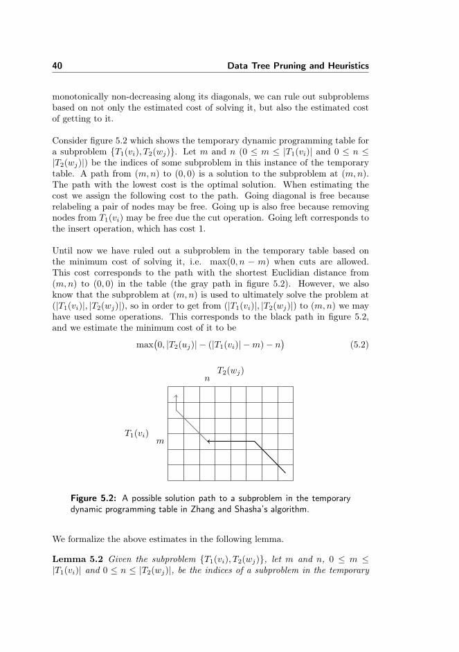
monotonically non-decreasing along its diagonals, we can rule out subproblemsbased on not only the estimated cost of solving it, but also the estimated costof getting to it.
Consider figure 5.2 which shows the temporary dynamic programming table fora subproblem {T1(vi), T2(wj)}. Let m and n (0 ≤ m ≤ |T1(vi)| and 0 ≤ n ≤|T2(wj)|) be the indices of some subproblem in this instance of the temporarytable. A path from (m,n) to (0, 0) is a solution to the subproblem at (m,n).The path with the lowest cost is the optimal solution. When estimating thecost we assign the following cost to the path. Going diagonal is free becauserelabeling a pair of nodes may be free. Going up is also free because removingnodes from T1(vi) may be free due the cut operation. Going left corresponds tothe insert operation, which has cost 1.
Until now we have ruled out a subproblem in the temporary table based onthe minimum cost of solving it, i.e. max(0, n − m) when cuts are allowed.This cost corresponds to the path with the shortest Euclidian distance from(m,n) to (0, 0) in the table (the gray path in figure 5.2). However, we alsoknow that the subproblem at (m,n) is used to ultimately solve the problem at(|T1(vi)|, |T2(wj)|), so in order to get from (|T1(vi)|, |T2(wj)|) to (m,n) we mayhave used some operations. This corresponds to the black path in figure 5.2,and we estimate the minimum cost of it to be
max(0, |T2(uj)| − (|T1(vi)| −m)− n
)(5.2)
m
n
T1(vi)
T2(wj)
Figure 5.2: A possible solution path to a subproblem in the temporarydynamic programming table in Zhang and Shasha’s algorithm.
We formalize the above estimates in the following lemma.
Lemma 5.2 Given the subproblem {T1(vi), T2(wj)}, let m and n, 0 ≤ m ≤|T1(vi)| and 0 ≤ n ≤ |T2(wj)|, be the indices of a subproblem in the temporary
5.2 Using Lower Bounds for Pruning 41
dynamic programming table of Zhang and Shasha’s algorithm. The minimumcost of the subproblem {T1(vi), T2(wj)} then is
max(0, |T2(wj)| − (|T1(vi)| −m)− n
)+ max
(0, n−m
)(5.3)
Proof. The best way to get from the nth column to the 0th column is n relabelswhich may be free. We can at most perform |n−m| relabels, so if n−m > 0 werequire n −m inserts, which have unit cost, otherwise we require m − n cuts,which are free. Same argument holds for the best way from (|T1(vi)|, |T2(wj)|)to (m,n). �
Adapting the algorithm to cuts has some drawbacks. As mentioned earlier, a lotfewer subproblems are ruled out from the permanent table. This is also the casein the temporary table in spite of our attempts to tighten it up with lemma 5.2.The main drawback is in fact in the temporary table where only subproblemsof the upper right and lower left corners are ruled out, so the impact diminishesas the difference in the size of the subtrees grows bigger.
In figure 5.2 on the preceding page a graphical comparison of the subproblemscomputed by the algorithms is shown. We see that a lot fewer subproblemsare needed in (b) compared to (c). If we were to show another temporary tablewhere T1(v) is a lot larger than T2(w), then it would be the same number of sub-problems required for (b) whereas it would be the same number of subproblemsruled out in (c). Clearly, this will have a negative effect on the execution timeof our adaption of the algorithm, because the size of a subtree in T1 generallyexceeds that of T2 in a pattern matching context.
5.2 Using Lower Bounds for Pruning
In the previous section we saw how to rule out subproblems based on a lowerbound obtained from the difference in the size of the components of the sub-problem. We anticipate that the unit cost algorithm adapted for cuts does notoutperform Zhang and Shasha’s original algorithm, so in this section we de-scribe a technique for pruning the data tree using the lower bound methodsfrom chapter 4.
We would like to remove subtrees that under no circumstances are a part of anoptimal mapping. If there is a pair of subtrees for which the lower bound ontheir tree edit distance with cuts is less than k, the given subtree in the datatree can not be removed. Using lower bounds ensure that we do not removesubtrees that are part of an optimal mapping unless the cost of the optimal

42 Data Tree Pruning and Heuristics
Permanent table
T1
T2
T1(v
)
T2(w)
(a) Algorithmusing keyroots.
T1
T2
T1(v
)
T2(w)
Temporary table(b) Fast unitcost algorithm.
T1
T2
T1(v
)
T2(w)
(c) Fast unitcost algorithmadapted forcuts.
Figure 5.3: Comparison of how subproblems are ruled out in the per-manent and temporary table of Zhang and Shasha’s algorithms. Whiteelements are computed subproblems.
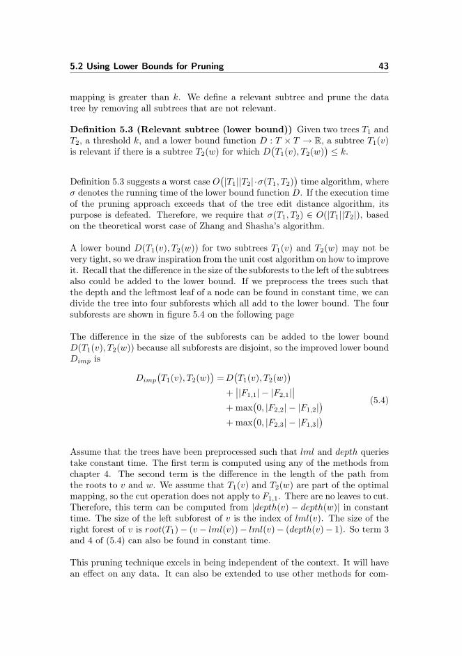
5.2 Using Lower Bounds for Pruning 43
mapping is greater than k. We define a relevant subtree and prune the datatree by removing all subtrees that are not relevant.
Definition 5.3 (Relevant subtree (lower bound)) Given two trees T1 andT2, a threshold k, and a lower bound function D : T × T → R, a subtree T1(v)is relevant if there is a subtree T2(w) for which D
(T1(v), T2(w)
)≤ k.
Definition 5.3 suggests a worst case O(|T1||T2| ·σ(T1, T2)
)time algorithm, where
σ denotes the running time of the lower bound function D. If the execution timeof the pruning approach exceeds that of the tree edit distance algorithm, itspurpose is defeated. Therefore, we require that σ(T1, T2) ∈ O(|T1||T2|), basedon the theoretical worst case of Zhang and Shasha’s algorithm.
A lower bound D(T1(v), T2(w)) for two subtrees T1(v) and T2(w) may not bevery tight, so we draw inspiration from the unit cost algorithm on how to improveit. Recall that the difference in the size of the subforests to the left of the subtreesalso could be added to the lower bound. If we preprocess the trees such thatthe depth and the leftmost leaf of a node can be found in constant time, we candivide the tree into four subforests which all add to the lower bound. The foursubforests are shown in figure 5.4 on the following page
The difference in the size of the subforests can be added to the lower boundD(T1(v), T2(w)) because all subforests are disjoint, so the improved lower boundDimp is
Dimp
(T1(v), T2(w)
)=D
(T1(v), T2(w)
)+∣∣|F1,1| − |F2,1|
∣∣+ max
(0, |F2,2| − |F1,2|
)+ max
(0, |F2,3| − |F1,3|
) (5.4)
Assume that the trees have been preprocessed such that lml and depth queriestake constant time. The first term is computed using any of the methods fromchapter 4. The second term is the difference in the length of the path fromthe roots to v and w. We assume that T1(v) and T2(w) are part of the optimalmapping, so the cut operation does not apply to F1,1. There are no leaves to cut.Therefore, this term can be computed from |depth(v) − depth(w)| in constanttime. The size of the left subforest of v is the index of lml(v). The size of theright forest of v is root(T1)− (v − lml(v))− lml(v)− (depth(v)− 1). So term 3and 4 of (5.4) can also be found in constant time.
This pruning technique excels in being independent of the context. It will havean effect on any data. It can also be extended to use other methods for com-
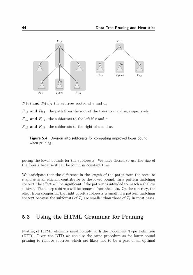
44 Data Tree Pruning and Heuristics
T1(v)F1,2 F1,3
F1,1
T2(w)F2,2 F2,3
F2,1
v
w
T1(v) and T2(w): the subtrees rooted at v and w,
F1,1 and F2,1: the path from the root of the trees to v and w, respectively,
F1,2 and F1,2: the subforests to the left if v and w,
F1,3 and F1,3: the subforests to the right of v and w.
Figure 5.4: Division into subforests for computing improved lower boundwhen pruning.
puting the lower bounds for the subforests. We have chosen to use the size ofthe forests because it can be found in constant time.
We anticipate that the difference in the length of the paths from the roots tov and w is an efficient contributor to the lower bound. In a pattern matchingcontext, the effect will be significant if the pattern is intended to match a shallowsubtree. Then deep subtrees will be removed from the data. On the contrary, theeffect from comparing the right or left subforests is small in a pattern matchingcontext because the subforests of T2 are smaller than those of T1 in most cases.
5.3 Using the HTML Grammar for Pruning
Nesting of HTML elements must comply with the Document Type Definition(DTD). Given the DTD we can use the same procedure as for lower boundpruning to remove subtrees which are likely not to be a part of an optimal
5.3 Using the HTML Grammar for Pruning 45
mapping. Consider the following definition of a relevant subtree. We remove allsubtrees that are not relevant.
Definition 5.4 (Relevant subtree (HTML grammar)) Given two trees T1
and T2, a subtree T1(v) is relevant if there is a node w in T2 such that the HTMLelement represented by w can be derived from the element represented by v fromthe DTD by applying one production rule or there is a relevant subtree T1(u)where u is a descendant of v.
The definition is recursive which is utilized by the algorithm. It traverses thenodes of the data tree in postorder. For each node it checks if there is a childthat is the root of a relevant subtree. If so, the current subtree is also relevant.If not it tests if there is a tag in T2 that is a possible descendant of the currentnode’s tag. To do this it is allowed to apply one rule from the DTD.
The traversal of the children of each node entails that each node is visited atmost two times. For each node in T1 each node in T2 is visited once. Finally,at most |T1| nodes are deleted. Thus, the running time of the algorithm is2|T1|+ |T1||T2| ∈ O
(|T1||T2|
).
We now discuss the expected efficiency of HTML pruning. If the providedpattern contains tags in the body branch of the HTML document, this approachwill remove at least the head branch, and vice versa. Also, inline elementscan not contain block elements, and most interactive elements can not containelements from any other group. For instance, all inline elements will be pruned ifthe pattern is sheer block elements. Another example: the select element canonly contain optgroup and option elements. So if the pattern is composed ofdiv and span tags, all select, and potentially many option tags, are removed.
Unfortunately, the restrictions posed by the DTD on basic layout elements arenot very strict. For instance, given a pattern of several div containers, it isunlikely that this is within a table cell, and it would have been nice to be ableto remove all tables from the data. Alas, table cells can contain div containersso this is not possible. If a transitional DTD is used, the restrictions becomeeven more vague, and this may also influence the efficiency of the approach.
In special cases, where there is no obvious subtree to match the pattern, thispruning approach may remove subtrees that are part of the optimal solution. Insuch cases the optimal solution may be to relabel many nodes to fit the pattern.The relabeled nodes may semantically be very different but be arranged similarto the pattern. Because of the semantic difference they are prone to beingremoved by HTML pruning.

46 Data Tree Pruning and Heuristics
5.4 Pre-selection of Subtrees
We have proposed two techniques for pruning the data tree, but in some casesthe effect from either of these may not be substantial. In this section we proposesome heuristics for selecting subtrees of the data tree based on the root of thepattern. When using XPaths for web scraping it is common to use the id orclass attribute (or any suitable attribute or CSS property) to select subtreeswhere the target data may possibly be. This is based on the assumption thatit is less likely that for instance the id of a tag changes than the path from theroot to the tag changes. We adopt this approach to approximate tree patternmatching.
We have identified three cases where the root of the pattern will map to a nodein the data tree with zero cost, because a mapping to any other node will conflictwith the semantic meaning of the HTML tags.
Case 1. If the root of the pattern is a body or head tag it is unlikely that itwill map to a node with another tag because the three mentioned tags areunique and only appear once each in the HTML document.
Case 2. If the root of the pattern has the id-attribute, it is unlikely that it willmap to a node representing tag with another id. Since the id uniquelyidentifies a tag it is unlikely that it will change due to a modification of awebsite layout. This of course depends on the extent of the modification.For example, it is not unlikely that a tag is removed when the layout ismodified, so this only applies to tags that can be identified as playing akey role in the layout of the website.
Case 3. If the root of the pattern is a tag with a restricted set of possibledescendants, it is unlikely that it will map to a node representing anothertag. Tags such as form and table is expected to contain certain tags, sorenaming either of these requires most of its descending tags to be renamedas well.
The three cases can be used to select subtrees by doing a linear search for nodesthat match the tag (case 1 and 3) or the id (case 2) of the root of the pattern.Because they are based on assumptions, using them for pre-selection of subtreescan result in sub optimal solutions.
Case 1 is the strongest assumption, but in practice it will at most eliminate thehead or body branch of the data tree. Case 2 requires the user to identify anelement with a key role in the layout. A web site often consists of a number
5.5 Linear Matching 47
of div containers given ids and styled using a Cascading Style Sheet (CSS).For the average user it can be difficult to determine how likely it is that forinstance a div container is discarded in a layout modification. Therefore, thiscase should only be used as a last resort. Case 3 only applies to a small set ofpatterns but when used it is subject to large reductions of the data tree.
5.5 Linear Matching
As we have seen in section 3.2 on pattern design, patterns naturally end up hav-ing an anchor of some length. Likewise, we have identified that many websitesuse a number of nested, styled div containers in order to create their visual ap-pearance. The resulting HTML tree therefore contains paths among its internalnodes where each node has exactly one child. If we apply pre-selection and theresult is a subtree with an anchor, there is a chance that the anchors of theselected subtree and the pattern will be part of a mapping with zero cost. Wecan exploit this by mapping nodes in a top-down manner for as long as the costof renaming nodes is zero.
Lemma 5.5 formalizes that a mapping obtained from linear matching is part ofan optimal mapping.
Lemma 5.5 (Linear matching) Let T1 and T2 be trees where nodes are givenpreorder indices. The lenght of the anchor of T1 is a1 and the length of theanchor of T2 is a2. Let γ be a unit cost function on the nodes, and let M be anoptimal mapping from T1 to T2. Let vi ∈ V (T1) and wi ∈ V (T2), then we have{
(vi, wi), 0 ≤ i ≤ min(a1, a2)∧γ(vi, wi) = 0∧(i = 0∨ (vi−1, wi−1) ∈M
)}⊆M
Proof. Let v = root(T1) and w = root(T2). It is sufficient to show that (v, w) ispart of an optimal mapping if γ(v, w) = 0, because we know from lemma 2.3 onpage 10 that the algorithm will recurse on T1−v and T2−w, and the proof thenholds recursively. Assume that the cost of relabeling v to w is 0, but there is amapping M ′ with cost c such that w maps to some other node v′ that descendsfrom v. Let d be the depth of v′, then 0 < d ≤ c. We can transform M ′ to amapping M ′′ that contains (v, w) by removing (v′, w) and inserting (v, w). Tochange the cost of the mapping accordingly, we need to subtract the depth of v′and the cost of deleting it. Thus, the cost of M ′′ is c− (d− 1). Since we knowthat d > 0 we see that M ′′, which contains the pair (v, w), is just as good orbetter than M ′. �
The advantage of this heuristic is that it is very fast. If no nodes match, only

48 Data Tree Pruning and Heuristics
the roots of the data and the pattern is compared, so the overhead is constant.If one or more nodes match, the overhead is O(height(T2)), but in return we geta reduction in both the data and the pattern before invoking the approximatetree pattern matching algorithm.
Chapter 6
Experiments
This chapter presents the results from conducting a range of experiments usingour implementation (described in appendix A).
6.1 Setup
The objective of the experiments is to
• compare execution time of Zhang and Shasha’s algorithm to our adaptionof their fast unit cost algorithm for cuts when used for web scraping,
• compare the lower bound methods,
• compare HTML grammar pruning and lower bound pruning using all lowerbound methods,
• substantiate the effect of the heuristic methods, and
• show how tolerant Zhang and Shasha’s algorithm is to changes in a webpage and compare it to XPath.
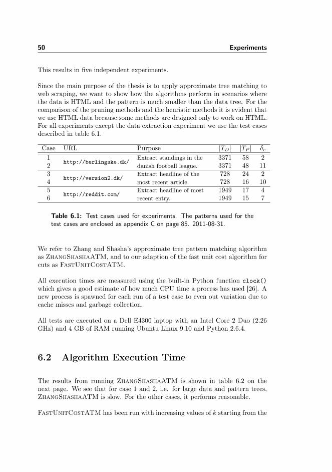
50 Experiments
This results in five independent experiments.
Since the main purpose of the thesis is to apply approximate tree matching toweb scraping, we want to show how the algorithms perform in scenarios wherethe data is HTML and the pattern is much smaller than the data tree. For thecomparison of the pruning methods and the heuristic methods it is evident thatwe use HTML data because some methods are designed only to work on HTML.For all experiments except the data extraction experiment we use the test casesdescribed in table 6.1.
Case URL Purpose |TD| |TP | δc
1http://berlingske.dk/
Extract standings in thedanish football league.
3371 58 22 3371 48 113
http://version2.dk/Extract headline of themost recent article.
728 24 24 728 16 105
http://reddit.com/Extract headline of mostrecent entry.
1949 17 46 1949 15 7
Table 6.1: Test cases used for experiments. The patterns used for thetest cases are enclosed as appendix C on page 85. 2011-08-31.
We refer to Zhang and Shasha’s approximate tree pattern matching algorithmas ZhangShashaATM, and to our adaption of the fast unit cost algorithm forcuts as FastUnitCostATM.
All execution times are measured using the built-in Python function clock()which gives a good estimate of how much CPU time a process has used [26]. Anew process is spawned for each run of a test case to even out variation due tocache misses and garbage collection.
All tests are executed on a Dell E4300 laptop with an Intel Core 2 Duo (2.26GHz) and 4 GB of RAM running Ubuntu Linux 9.10 and Python 2.6.4.
6.2 Algorithm Execution Time
The results from running ZhangShashaATM is shown in table 6.2 on thenext page. We see that for case 1 and 2, i.e. for large data and pattern trees,ZhangShashaATM is slow. For the other cases, it performs reasonable.
FastUnitCostATM has been run with increasing values of k starting from the

6.3 Lower Bound Methods 51
Case ZhangShashaATM1 67.99 s2 34.37 s3 1.54 s4 1.21 s5 4.39 s6 4.57 s
Table 6.2: Execution times of Zhang and Shasha’s approximate treepattern matching algorithm.
optimal tree edit distance. The results are shown in table 6.3 on the followingpage. As anticipated, the algorithm does not outperform ZhangShashaATM.
6.3 Lower Bound Methods
The lower bound methods have been tested on the 6 test cases and the resultsare shown in table 6.4 on the next page. We see that the only test where theapproximation is close to the optimal edit distance with cuts δc is when we usethe Euler string distance in case 3. This indicates that the methods are unfit foruse as an approximation of the cost of matching a HTML pattern to a HTMLtree.
The lower bound methods were developed with the application to pruning inmind. In our pruning algorithm the methods are applied to all pairs of subtreesof two trees T1 and T2. Therefore, we have run the methods on all pairs of sub-trees in the 6 cases and accumulated the distances. The results are comparedto the accumulated tree edit distance
∑δc =
∑∀(v,w)∈V (T1)×V (T2) δc(v, w) be-
tween all pairs of subtrees. Based on the results shown in table 6.5 on page 53,the q-gram tree distance, where q = 1, and the Euler string distance are thetightest lower bound approximations.
6.4 Pruning Methods
We want to determine how effective the pruning methods are on HTML data.Our approach is to compare the size of the data tree before and after a pruningmethod has been applied and measure the CPU time of executing the pruning
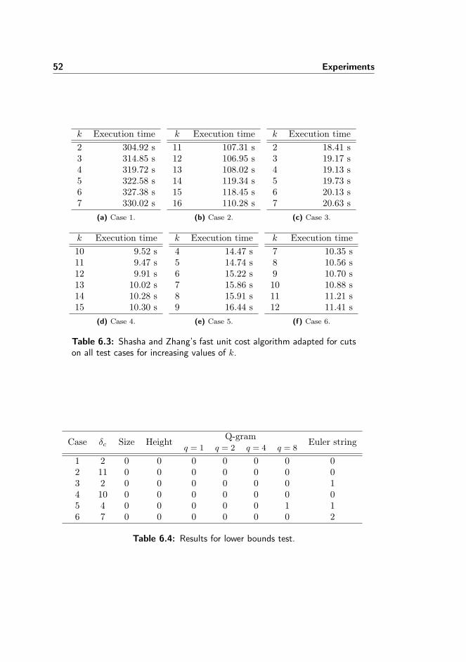
52 Experiments
k Execution time2 304.92 s3 314.85 s4 319.72 s5 322.58 s6 327.38 s7 330.02 s
(a) Case 1.
k Execution time11 107.31 s12 106.95 s13 108.02 s14 119.34 s15 118.45 s16 110.28 s
(b) Case 2.
k Execution time2 18.41 s3 19.17 s4 19.13 s5 19.73 s6 20.13 s7 20.63 s
(c) Case 3.
k Execution time10 9.52 s11 9.47 s12 9.91 s13 10.02 s14 10.28 s15 10.30 s
(d) Case 4.
k Execution time4 14.47 s5 14.74 s6 15.22 s7 15.86 s8 15.91 s9 16.44 s
(e) Case 5.
k Execution time7 10.35 s8 10.56 s9 10.70 s10 10.88 s11 11.21 s12 11.41 s
(f) Case 6.
Table 6.3: Shasha and Zhang’s fast unit cost algorithm adapted for cutson all test cases for increasing values of k.
Case δc Size Height Q-gram Euler stringq = 1 q = 2 q = 4 q = 8
1 2 0 0 0 0 0 0 02 11 0 0 0 0 0 0 03 2 0 0 0 0 0 0 14 10 0 0 0 0 0 0 05 4 0 0 0 0 0 1 16 7 0 0 0 0 0 0 2
Table 6.4: Results for lower bounds test.
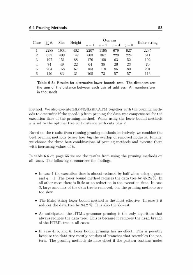
6.4 Pruning Methods 53
Case∑δc Size Height Q-gram Euler string
q = 1 q = 2 q = 4 q = 8
1 2288 1904 402 2207 1195 679 627 22352 657 409 147 603 367 229 224 6113 197 151 88 179 100 63 52 1924 74 49 22 64 38 26 23 705 204 158 67 183 118 86 80 2016 120 83 31 105 73 57 57 116
Table 6.5: Results for alternative lower bounds test. The distances arethe sum of the distance between each pair of subtrees. All numbers arein thousands.
method. We also execute ZhangShashaATM together with the pruning meth-ods to determine if the speed-up from pruning the data tree compensates for theexecution time of the pruning method. When using the lower bound methodsk is set to the optimal tree edit distance with cuts plus 2.
Based on the results from running pruning methods exclusively, we combine thebest pruning methods to see how big the overlap of removed nodes is. Finally,we choose the three best combinations of pruning methods and execute themwith increasing values of k.
In table 6.6 on page 55 we see the results from using the pruning methods onall cases. The following summarizes the findings.
• In case 1 the execution time is almost reduced by half when using q-gramand q = 1. The lower bound method reduces the data tree by 45.24 %. Inall other cases there is little or no reduction in the execution time. In case3, large amounts of the data tree is removed, but the pruning methods aretoo slow.
• The Euler string lower bound method is the most effective. In case 3 itreduces the data tree by 94.2 %. It is also the slowest.
• As anticipated, the HTML grammar pruning is the only algorithm thatalways reduces the data tree. This is because it removes the head branchof the HTML tree in all cases.
• In case 4, 5, and 6, lower bound pruning has no effect. This is possiblybecause the data tree mostly consists of branches that resembles the pat-tern. The pruning methods do have effect if the pattern contains nodes

54 Experiments
that are not used very frequently in the data as in case 1, or the patterncontains many different nodes as in case 3.
Based on these findings we have combined the size, height, q-gram (q = 1), andHTML pruning methods for a similar round of tests. However, these tests haveonly been run on case 1, 2, and 3 where the pruning methods proved to have aneffect when run exclusively. The results are shown in table 6.7 on page 56, andare summarized below.
• There is an overlap in the data removed by the pruning methods. However,case 3 shows that the overlap between the size and q-gram methods is sosmall that the combination of the two is fast.
• Combining the pruning methods generally result in an increase in theamount of removed data, but it is too small to compensate for the overheadof using two pruning methods.
The effectiveness of the lower bound pruning methods depends on the thresholdk. We have selected 1-gram, size+height, and size+1-gram as the three bestpruning methods, and have executed them on case 1 (figure 6.1 on page 57)and case 3 (figure 6.2 on page 57) for increasing values of k. In both cases theoptimal tree edit distance with cuts is 2.
Figure 6.1 shows that for small values of k, the size+1-gram combination ismarginally better than using just 1-grams. Most notable is the increase inexecution time when k is changed from 6 to 7. For values greater than 7 thepruning methods are useless. The same tendency is seen in figure 6.2, but thebreak even is between k = 4 and k = 5. The latter figure also shows that if thek-value provided is not sufficiently tight, then the pruning methods may addsignificant overhead. In practice we should only use the pruning methods if wecan provide a tight k-value.
6.5 Heuristics
The results from using pre-selection and linear matching on the 6 test cases areshown in table 6.8 on page 58. We see that pre-selection selects a subtree towork on in case 2, 3, and 6. The patterns used in these cases have a table, body,and a div tag with an id attribute, respectively, as roots. Linear matching hasno influence on the test cases. The execution time of the heuristic methods isomitted from the table because it is smaller than 0.01 seconds for all cases.

6.5 Heuristics 55
Case
Non
eLo
wer
boun
dHTML
Size
Hei
ght
q-gr
am(q
=1)
q-gr
am(q
=2)
q-gr
am(q
=4)
Eul
erst
ring
1-
5.68
%1.
37%
45.2
4%
45.2
4%
45.2
4%
45.2
4%
0.9%
-0.
05s
0.79
s5.
09s
8.65
s14.4
s33.6
6s
0.04
s62.0
6s
58.2
5s
61.9
5s
35.4
6s
39.6
8s
46.5
4s
63.9
2s
62.0
3s
2-
0.31
%0.
31%
0.31
%0.
31%
0.31
%0.
31%
0.91
%-
0.04
s0.
33s
2.46
s4.
09s
6.83
s7.
45s
0.04
s31.7
6s
31.8
4s
31.6
9s
34.3
7s
36.7
6s
40.4
7s
39.5
9s
31.2
3s
3-
10.6
4%
7.87
%51.2
4%
75.0
%12.9
8%
94.2
%2.
62%
-0.
01s
0.11
s0.
74s
1.24
s2.
22s
5.37
s<
0.01
s1.
45s
1.37
s1.
50s
1.36
s1.
53s
3.45
s5.
44s
1.45
s
4-
0.0%
0.0%
0.0%
0.0%
0.0%
0.0%
2.62
%-
<0.
01s
0.03
s0.
13s
0.23
s0.
39s
0.32
s<
0.01
s1.
22s
1.22
s1.
16s
1.26
s1.
37s
1.54
s1.
43s
1.14
s
5-
0.0%
0.0%
0.0%
0.0%
0.0%
0.0%
3.42
%-
0.02
s0.
08s
0.38
s0.
61s
0.92
s1.
07s
0.01
s4.
42s
4.41
s4.
51s
5.15
s5.
16s
5.42
s5.
56s
4.36
s
6-
0.0%
0.0%
0.0%
0.0%
0.0%
0.0%
3.42
%-
0.02
s0.
08s
0.31
s0.
51s
0.73
s0.
79s
0.01
s4.
53s
4.55
s4.
66s
4.91
s5.
20s
5.49
s5.
42s
4.50
s
Table
6.6:
Results
from
prun
ingmetho
dtests.
Firstrow
ofeach
case
ispercentage
ofdata
tree
removed.Second
row
istheexecutiontim
eof
theprun
ingmetho
d.Third
row
istheexecutiontim
eof
theprun
ingmetho
dfollowed
byZhangShash
aAT
M.
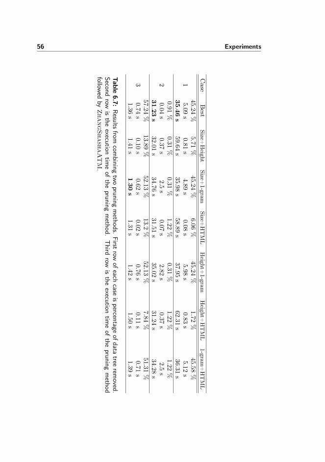
56 Experiments
Case
Best
Size+H
eightSize+
1-gramSize+
HT
ML
Height+
1-gramH
eight+H
TM
L1-gram
+H
TM
L
145.24
%5.71
%45.24
%6.06
%45.24
%1.72
%45.58
%5.09
s0.81
s4.89
s0.08
s5.98
s0.83
s5.12
s35.46
s59.64
s35.98
s58.89
s37.95
s62.31
s36.31
s
20.91
%0.31
%0.31
%1.22
%0.31
%1.22
%1.22
%0.04
s0.37
s2.5
s0.07
s2.82
s0.37
s2.5
s31.23
s32.01
s34.76
s31.51
s35.02
s31.24
s34.28
s
357.24
%13.89
%52.13
%13.2
%52.13
%7.84
%51.31
%0.74
s0.10
s0.62
s0.02
s0.76
s0.11
s0.71
s1.36
s1.41
s1.30
s1.31
s1.42
s1.50
s1.39
s
Table
6.7:Results
fromcom
biningtwopruning
methods.
Firstrow
ofeach
caseispercentage
ofdata
treerem
oved.Second
rowis
theexecution
timeof
thepruning
method.
Third
rowis
theexecution
timeof
thepruning
method
followed
byZhangShash
aAT
M.
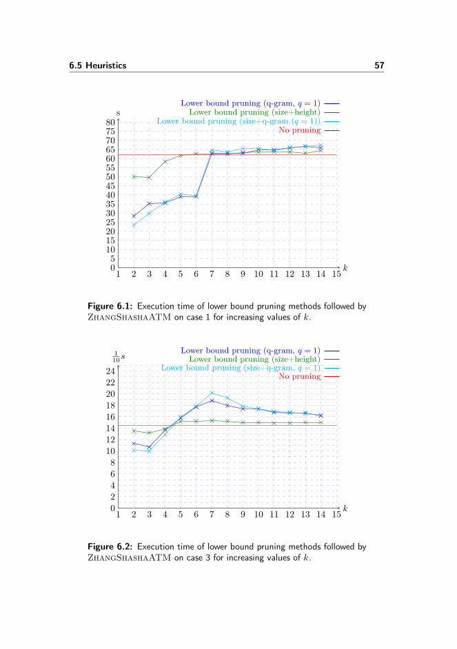
6.5 Heuristics 57
k
s
1 2 3 4 5 6 7 8 9 10 11 12 13 14 1505101520253035404550556065707580
Lower bound pruning (q-gram, q = 1)Lower bound pruning (size+height)
Lower bound pruning (size+q-gram (q = 1))No pruning
Figure 6.1: Execution time of lower bound pruning methods followed byZhangShashaATM on case 1 for increasing values of k.
k
110s
1 2 3 4 5 6 7 8 9 10 11 12 13 14 15024681012141618202224
Lower bound pruning (q-gram, q = 1)Lower bound pruning (size+height)
Lower bound pruning (size+q-gram, q = 1)No pruning
Figure 6.2: Execution time of lower bound pruning methods followed byZhangShashaATM on case 3 for increasing values of k.

58 Experiments
Case None Pre-selection Pre-selection and Linear Matching
1 - 0.0 % 0.0 %62.97 s 63.19 s 63.45 s
2 - 99.75 % 99.75 %32.09 s 0.25 s 0.25 s
3 - 3.24 % 3.24 %1.3 s 1.05 s 1.04 s
4 - 0.0 % 0.0 %0.99 s 0.98 s 1.0 s
5 - 0.0 % 0.0 %4.36 s 4.33 s 4.38 s
6 - 56.07 % 56.07 %4.51 s 0.99 s 0.98 s
Table 6.8: Results from using the heuristics with ZhangShashaATM.The first row for each case is the percentage of the data tree removedand the second row is the execution time of ZhangShashaATM plusthe overhead from using the heuristic.
6.6 Data Extraction
Zhang and Shasha’s algorithm extracts the correct data from the 6 test casesin table 6.1 on page 50, so to compare the behaviour of the algorithms we haveconstructed the simple web page shown in figure 6.3 on the next page. The webpage consists of 5 div containers which are given different class attributes. Thetwo innermost divs contain a bold text in a paragraph and three bullet points.We make 8 changes to the web page. The changes cover some possible changesin markup that a website can be subject to.
The target of the experiment is to extract the text in the green div. The orangediv is present to mislead the algorithms. We compare our algorithms to theresult from applying the following two different XPaths to the web page.
XPath pattern 1 XPath pattern 2//div/div[1]/div/p/strong |//div/div[1]/div/ul/li
//div[@class=’green’]/p/strong |//div[@class=’green’]/ul/li
We also include Zhang’s algorithm for the isolated-subtree mapping in the com-parison. Although it was rejected for not being suited for web scraping inchapter 3 we want to take this opportunity to investigate if there are more caseswhere it fails to locate the correct data. The pattern used with the approximate
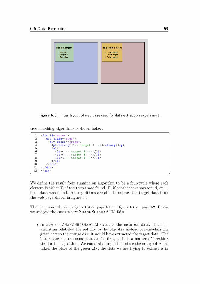
6.6 Data Extraction 59
Figure 6.3: Initial layout of web page used for data extraction experiment.
tree matching algorithms is shown below.� �1 <div id="outer">2 <div class="blue">3 <div class="green">4 <p><strong ><!-- target 1 --></strong ></p>5 <ul>6 <li><!-- target 2 --></li>7 <li><!-- target 3 --></li>8 <li><!-- target 4 --></li>9 </ul>
10 </div>11 </div>12 </div>� �
We define the result from running an algorithm to be a four-tuple where eachelement is either T , if the target was found, F , if another text was found, or −,if no data was found. All algorithms are able to extract the target data fromthe web page shown in figure 6.3.
The results are shown in figure 6.4 on page 61 and figure 6.5 on page 62. Belowwe analyze the cases where ZhangShashaATM fails.
• In case (c) ZhangShashaATM extracts the incorrect data. Had thealgorithm relabeled the red div to the blue div instead of relabeling thegreen div to the orange div, it would have extracted the target data. Thelatter case has the same cost as the first, so it is a matter of breakingties for the algorithm. We could also argue that since the orange div hastaken the place of the green div, the data we are trying to extract is in

60 Experiments
fact the contents of the orange div. The interpretation depends on thecontext. The second XPath pattern extracts the data because it targetsthe green div on its class name.
• In case (f) the paragraph and the unordered list have switched place.We know that ZhangShashaATM can not match both because it wouldviolate the definition of a mapping. Therefore, it chooses to remove thesmallest subtree of the two. Again, we could also argue that the originaltarget 1 has been removed and a new text has been inserted, in which casethe result from the algorithm is correct. Both XPath patterns extract thedata because they are a concatenation of two paths.
• In case (g) the incorrect data is extracted. The change is radical and onemight argue that in such cases the algorithm is not supposed to find amatching. The XPaths also fails.
The results show that IsolatedSubtreeATM locates the data in the samecases as ZhangShashaATM.

6.6 Data Extraction 61
Algorithm ResultXPath 1 (−,−,−,−)XPath 2 (T, T, T, T )ZhangShashaATM (T, T, T, T )IsolatedSubtreeATM (T, T, T, T )
(a)
Algorithm ResultXPath 1 (−,−,−,−)XPath 2 (T, T, T, T )ZhangShashaATM (T, T, T, T )IsolatedSubtreeATM (T, T, T, T )
(b)
Algorithm ResultXPath 1 (F, F, F, F )XPath 2 (T, T, T, T )ZhangShashaATM (F, F, F, F )IsolatedSubtreeATM (F, F, F, F )
(c)
Algorithm ResultXPath 1 (F, F, F, F )XPath 2 (T, T, T, T )ZhangShashaATM (T, T, T, T )IsolatedSubtreeATM (T, T, T, T )
(d)
Figure 6.4: Results from data extraction experiment (part 1).

62 Experiments
Algorithm ResultXPath 1 (T,−,−,−)XPath 2 (T,−,−,−)ZhangShashaATM (T, T, T, T )IsolatedSubtreeATM (T, T, T, T )
(e)
Algorithm ResultXPath 1 (T, T, T, T )XPath 2 (T, T, T, T )ZhangShashaATM (F, F, F, F )IsolatedSubtreeATM (F, F, F, F )
(f)
Algorithm ResultXPath 1 (T,−,−,−)XPath 2 (T,−,−,−)ZhangShashaATM (F, F, F, F )IsolatedSubtreeATM (F, F, F, F )
(g)
Algorithm ResultXPath 1 (T, T, T, T )XPath 2 (−,−,−,−)ZhangShashaATM (T, T, T, T )IsolatedSubtreeATM (T, T, T, T )
(h)
Figure 6.5: Results from data extraction experiment (part 2).
Chapter 7
Discussion
In this chapter we will consider our findings as a whole and discuss how theyare best combined to a solution for web scraping. The discussion will focus onchoosing an algorithm and suitable pruning methods, and the consequences thechoices will have.
7.1 Algorithms
In the litterature, web scraping using approximate tree pattern matching isachieved using algorithms that create a top-down mapping, because the focusis on generating the pattern from a set of web pages. However, there are caseswhere the data to be extracted resides on just one web page, so the need for amore versatile solution is present.
We have considered Zhang and Shasha’s algorithm and Zhang’s isolated-subtreealgorithm for web scraping, because unlike the top-down mapping, they imposeno requirements on the pattern. Although fictitious, the Reddit example showsthat there is a simple case of change in the markup where the isolated-subtreealgorithm fails to locate the targeted data. We regard this example as a changethat is likely to happen due to the fact that it is a simple way of adding or

64 Discussion
removing visual attributes to a collection of tags. Furthermore, the data ex-traction experiment shows that there are no cases where the isolated-subtreealgorithm locates data that Zhang and Shasha’s algorithm was unable to lo-cate. To meet our aim that the solution should be as error tolerant as possible,the isolated-subtree algorithm is not an option for web scraping.
That being said, the data extraction experiment shows a couple of cases whereZhang and Shasha’s algorithm extract incorrect data. It goes to show that theoptimal solution is not always what we intuitively would call the correct solution.To deal with this, we could guide the algorithm using the cost function. However,this is not covered in this thesis because the pruning methods assume that aunit cost function is used. On the other hand, the experiment also shows thatthe correct data is found in 7 out of the 8 cases using either the evaluation of thesecond XPath or approximate tree pattern matching. This suggests a hybridbetween the methods where e.g. approximate tree pattern matching is used asfallback if at least one of the XPaths yields an empty result set.
We have shown that Shasha and Zhang’s fast unit cost algorithm is not suited forpattern matching when the pattern is small compared to the data tree. Theremay still be a speed-up compared to Zhang and Shasha’s algorithm in caseswhere the pattern is close to the size of the data tree. To be faster, the fast unitcost algorithm must rule out about as many subproblems as ruled out whenZhang and Shasha’s algorithm selects keyroots.
7.2 Lower Bound Methods
The cut operation has made it difficult to obtain tight lower bounds. Twonovel approximation methods from the litterature, the PQ-gram distance andthe binary branch distance, were not tranformable to produce lower bounds atall, and the size and height methods only apply if the pattern tree is bigger orhigher than the data tree.
The tightest lower bounds are obtained from the Euler string distance and q-gram distance where q = 1. The two methods are in fact quite similar. When q =1 we check if the nodes in the pattern tree are also present in the data tree. Thisis basically the same that happens when comparing the Euler strings becausethe delete operation in the string edit distance algorithm is free. However, theorder of the nodes in the Euler string embeds some information about the treestructure, so the Euler string distance gives slightly better approximations. Inreturn it is slow.

7.3 Pruning Method and Heuristics 65
Our experiments show that if the data is HTML and the pattern is found oneor more times in the data, the methods are poor approximations. However,further experiments show that if the cost of an optimal mapping of a patternto the data is high, the approximations become better. This is useful when themethods are used in our pruning algorithm.
7.3 Pruning Method and Heuristics
We lower bound pruning algorithm is independant of the type of data the treemodels. Our experiments show that when the data is HTML the combinationbetween the size and 1-gram distance lower bound methods are the most effectiveas long as the threshold k is reasonably tight.
An important property of the algorithm is that branches used in an optimalsolution is not removed. The drawback of the algorithm is its running time,which is O
(|T1||T2| ·σ(T1, T2)
), where σ(T1, T2) is the running time of the lower
bound method used. If using the Euler string distance with the algorithm, therunning time becomes O
(|T1|2|T2|2
), which is worse than the actual running
time of Zhang and Shasha’s algorithm. However, from our experiments we seethat the constant factor of overhead of the algorithm is little, so there are caseswhere pruning is beneficial and cases where the data tree is not reduced but theoverhead is negligible.
The lower bound pruning algorithm becomes more effective when the pattern islarge and has many nodes with distinct labels. However, if it is too large andpruning fails to reduce the data tree significantly, the whole process is sloweddown by both the pruning algorithm and subsequently by the approximate treepattern matching algorithm.
Our experiments show that the HTML grammar pruning algorithm is not veryeffective. However, the patterns used in the tests consist mostly of generic blockand inline, so the algorithm may become more effective if more diverse patternsare used. HTML inherits a lot of its properties from XML, so the algorithmis applicable to any tree model of semi-structured data with a DTD. In otherdomains, the algorithm may also be more effective. It is not guaranteed not toremove a branch that is part of an optimal solution, but for sufficiently largepatterns, we regard it as unlikely.
Finally, we have defined some heuristics for reducing the data tree. Pre-selectionyields large reductions in the size of the data tree. To take advantage of theheuristic we must strive to select a pattern where the root is either the body, the
66 Discussion
head, a table or a form tag or has the id attribute. However, the size of thepattern should not be too small. If pre-selection fails, the node that is expectedto map to the root of the pattern should not be too deep because this may resultin incorrect data being extracted. Therefore, the pattern should have an anchorof suitable length.
Linear matching is only applicable in a limited set of cases. There may be somesubtle differences in the mapping of the nodes in the anchors compared to themapping obtained from using Zhang and Shasha’s algorithm, but since we oftenwant to extract data from leaf nodes (or deep nodes) in the pattern, this shouldnot influence the outcome when used for web scraping.
Chapter 8
Conclusion
The aim of this thesis was to develop a fast and error tolerant solution for webscraping based on the tree edit distance without imposing any restrictions onthe pattern. The litterature treats web scraping as the second phase in a two-phase procedure, where the first phase deals with learning a pattern. If the setof web pages to learn from is not sufficiently large, the web scraping phase willfail because algorithms for the top-down mapping are used. Since we often wantto extract data from just one web page, the methods from the litterature areinadequate.
First, we proposed using an algorithm for the optimal mapping or an algorithmfor the isolated-subtree mapping. We gave an example of a simple and likelychange to the markup of a web page that made the algorithm for the isolated-subtree mapping fail. In our experiments, the result from the algorithm forthe optimal mapping and the algorithm for the isolated-subtree mapping wasthe same. Based on the first example, the isolated-subtree mapping is not aptfor web scraping. Among the algorithms for the optimal mapping, Zhang andShasha’s algorithm is the most suited because its running time depends on theheight of the input trees, which generally is low for HTML trees.
We adapted Shasha and Zhang’s fast unit cost tree edit distance algorithm topattern matching, but our experiments confirmed that the fourth edit operation,cut, which is required for pattern matching, makes it difficult to rule out a
68 Conclusion
significant number of subproblems. However, the work on the algorithm servedas inspiration for the two pruning algorithms that were developed.
The lower bound pruning algorithm extends the technique from the fast unit costalgorithm to prune the data tree prior to running an approximate tree patternmatching algorithm. In particular, it uses one of the lower bound methodsthat were developed from novel tree edit distance approximation methods foundin the litterature. Transforming these methods to produce tight lower boundapproximations for the tree edit distance with cuts proved to be difficult becauseof the issue of distinguishing between the free cut operation and the non-freedelete operation when comparing parts of the trees. The second algorithm usesthe HTML grammar from the DTD to exclude branches of the data tree. Of thetwo algorithms, the lower bound pruning algorithm is the most effective, giventhat the 1-gram distance is used as lower bound method. It is also the slowestbecause the lower bound methods are slow.
Our experiments showed that in one case, the data tree could be reduced by 95% using the lower bound pruning algorithm with the Euler string distance lowerbound method. In another case, the execution time was reduced from 62 secondsto 35 seconds due to pruning using the lower bound pruning algorithm and the1-gram distance lower bound method. In both cases the algorithm tolerated twomore errors than the cost of the optimal mapping. Furthermore, our experimentsshowed that the algorithm needs to be provided with a relatively small value ofk in order to be beneficial.
Algorithms, pruning algorithms, and lower bound methods were implementedin Python such that they could be combined arbitrarily for the experiments.
8.1 Further Work
The data extraction experiment showed that the there are cases where the ap-proximate tree pattern matching algorithm extracts incorrect data. To avoidthis and thus cover more cases, a final solution requires more work.
We only briefly discussed how to utilize this technique for web scraping when wewant to extract several matches of a pattern. Since this is a common use casein web scraping, it will require some further work to determine how to achievethis effectively.
We also believe that there are faster and better methods for finding lower boundsfor the tree edit distance with cuts that are waiting to be uncovered.
Bibliography
[1] Tatsuya Akutsu. A relation between edit distance for ordered trees and editdistance for Euler strings. Information Processing Letters, Vol. 100, Issue3, 105–109, 2006.
[2] Nikolaus Augsten, Michael Böhlen, Johann Gamper. The pq-gram distancebetween ordered labeled trees. ACM Trans. Database Syst., Vol. 35, ACM,New York, 24:1–4:36, 2010.
[3] Philip Bille. A survey on tree edit distance and related problems. Theor.Comput. Sci, Vol. 337, 217–239, 2005.
[4] Sudarshan S. Chawathe. Comparing Hierarchical Data in External Memory.In Proceedings of the Twenty-fifth International Conference on Very LargeData Bases, Morgan Kaufmann Publishers Inc, 90–101, 1999.
[5] Thomas H. Cormen, Charles E. Leiserson, Ronald L. Rivest, Clifford Stein.Introduction to Algorithms (2nd ed.). MIT Press and McGraw-Hill 2001.ISBN 0-262-53196-8.
[6] Erik D. Demaine, Shay Mozes, Benjamin Rossman, and Oren Weimann. AnOptimal Decomposition Algorithm for Tree Edit Distance. ACM Transac-tions on Algorithms, Vol. 6, No. 1, Article 2, 2009.
[7] Erich Gamma, Richard Helm, Ralph Johnson, John Vlissides. Design Pat-terns – Element of Reusable Object-Oriented Software. Addison-Wesley1995. ISBN 0-201-63361-2.
[8] Yeonjung Kim, Jeahyun Park, Teahwan Kim, Joongmin Choi. Web Infor-mation Extraction by HTML Tree Edit Distance Matching. In Proceedings

70 BIBLIOGRAPHY
of the 2007 International Conference on Convergence Information Tech-nology, pages 2455–2460, IEEE Computer Society, Washington, DC, USA,2007.
[9] P.N. Klein. Computing the edit-distance between unrooted ordered trees. InProceedings of the 6th annual European Symposium on Algorithms (ESA)1998., pages 91–102. Springer-Verlag, 1998.
[10] Donald Erwin Knuth. The Art of Computer Programming: Volume 1, Fun-damental Algorithms (section 2.3.2, Binary Tree Representation of Trees).Addison-Wesley, 1997. ISBN 0-201-89683-4.
[11] Davi De Castro Reis, Reis Paulo, Alberto H. F. Laender, Paulo B. Goglher,Altrigran S. da Silva. Automatic Web News Extraction Using Tree EditDistance. In Proceedings of World Wide Web Conference (WWW04), NewYork, USA, 2004.
[12] Thorsten Richter. A new algorithm for the ordered tree inclusion prob-lem. In Proceedings of the 8th Annual Symposium on Combinatorial Pat-tern Matching (CPM), in Lecture Notes of Computer Science (LNCS), Vol.1264, Springer, 150–166, 1997.
[13] Stanley M. Selkow. The tree-to-tree editing problem. Information Process-ing Letters, 6(6):184–186, 1977.
[14] Dennis Shasha and Kaizhong Zhang. Fast algorithms for the unit cost edit-ing distance between trees. Journal of Algorithms, 11:581–621, 1990.
[15] Kuo-Chung Tai. The tree-to-tree correction problem. Journal of the Asso-ciation for Computing Machinery (JACM), 26:422–433, 1979.
[16] Rui Yang, Panos Kalnis, Anthony K. H. Tung. Similarity evaluation ontree-structured data. Proceedings of the 2005 ACM SIGMOD internationalconference on Management of data, ACM, Baltimore, Maryland, 754–765,2005.
[17] Esko Ukkonen. Approximate string matching with q-grams and maximalmatches. Theoretical Computer Science 1, 191–211, 1994.
[18] Gabriel Valiente. An efficient bottom-up distance between trees. In Pro-ceedings of the 8th International Symposium of String Processing and In-formation Retrieval, Press, 212–219, 2001.
[19] Kaizhong Zhang, Dennis Shasha, Jason T. L. Wang. Approximate TreeMatching in the Presence of Variable Length Don’t Cares. Journal of Al-gorithms, 16:33–66, 1993.
BIBLIOGRAPHY 71
[20] Lin Xu, Curtis Dyreson. Approximate retrieval of XML data with ApproX-Path. In Proceedings of the nineteenth conference on Australasian database- Volume 75, pages 85–96, ADC ’08, Gold Coast, Australia, 2007.
[21] Wuu Yang. Identifying Syntactic Differences Between Two Programs. Soft-ware – Practice and Experience, 21:739–755, 1991.
[22] Kaizhong Zhang and Dennis Shasha. Simple fast algorithms for the editingdistance between trees and related problems. SIAM Journal of Computing,18:1245–1262, 1989.
[23] Kaizhong Zhang. Algorithms for the constrained editing problem betweenordered labeled trees and related problems. Pattern Recognition, 28:463–474, 1995.
Web sites
[24] Algorithm Implementation/Strings/Levenshtein distance – Wikibooks,open books for an open world.http://en.wikibooks.org/wiki/Algorithm_implementation/Strings/Levenshtein_distance#Python.2011-07-24.
[25] HTML 4.01 Transitional Document Type Definition.http://www.w3.org/TR/html401/sgml/loosedtd.html.2011-07-26.
[26] Time access and conversions – Python documentation.http://docs.python.org/library/time.html#time.clock.2011-08-31.
[27] Wikipedia. Metric (mathematics).http://en.wikipedia.org/wiki/Metric_(mathematics).2011-08-09.
[28] XPath Syntax.http://www.w3schools.com/Xpath/xpath_syntax.asp.2011-08-12.

72 BIBLIOGRAPHY

Appendix A
Implementation
In this chapter we give a brief overview of the implementation with emphasison the overall design and the implementation of the approximate tree patternmatching algorithms.
A.1 Design
We have implemented a number of algorithms, the lower bound and pruningmethods, and the heuristics described in this report. The implementation isin Python (version 2.6.4) which enables easy integration with for instance webservices written in Python. The result is a Python package with a fairly simpleAPI.
The functional requirements to the package is that it should be possible to
• combine pruning methods, linear matching, and pre-selection arbitrarily,and
• easily use it with other applications.

74 Implementation
To achieve the first goal, the pruning methods, linear matching, and pre-selectionhas been implemented as decorators for the algorithms∗. Any number of deco-rators can be wrapped around the algorithm in arbitrary order.
Using decorators introduce an overhead besides the extra functionality. Theinput trees must be preprocessed for each decorator because the trees may havebeen manipulated by a previous decorator. Particularly when adding severalLowerBoundPruning decorators the superflous tree preprocessing is done.
To make the algorithms usable for many purposes they operate on a genericdatastructure. To use the algorithm for a specific purpose such as web scraping,the calling application either has to be designed to use the generic datastructure,or define a context for the algorithm†, which must create a mapping between thegeneric datastructure and the one used by the calling application. The latteroption introduces some extra computation from creating the mapping betweenthe datastructures. However, we opt for the context approach because we wantto use the lxml‡ library for parsing HTML.
Algorithms, decorators, lower bound methods, and cost functions are subclassesof base classes that define the minimum requirement for functions in order tobe used with the rest of the package§.
A class diagram is shown in figure A.1 on the facing page. For the sake of clarity,private attributes and empty constructors for non-abstract classes are omitted.If no constructor is specified, it is inherited from its superclass.
A.2 Modules
The implementation consists of five Python modules which will be described inthis section.
∗The decorator pattern [7, pp. 175] allows functionality to be added transparently to acore function which in this case is the algorithm.†The purpose of the context pattern [7, pp. 317] is to be able reuse an implementation of
an algorithm in other applications without having to redeclare types, etc.‡lxml is Python library for parsing and processing XML and HTML. http://lxml.de/.§This is sometimes referred to as the strategy pattern, but because Python is typeless,
abstract classes are considered superflous. We opt to use it anyway for the sake of clarity forfuture contributors.

A.2 Modules 75
Figu
reA.1:Class
diagram.

76 Implementation
A.2.1 algorithms
This module contains implementations of the algorithms and the unit cost func-tion. The Algorithm class defines the interface used by all algorithms. Analgorithm is executed by invoking its object. Subsequently, the results can beretrieved from the functions get_distance() and get_edit_script(). Anoverview of the implemented algorithms is given in table A.1.
Class AlgorithmZhangShasha Zhang and Shasha’s algorithm [22]ZhangShashaATM Zhang and Shasha’s algorithm modified for cuts [22]ZhangShashaUC Shasha and Zhang’s fast unit cost algorithm [14]ZhangShashaUCATM Shasha and Zhang’s fast unit cost algorithm modified
for cuts (section 5.1.2 on page 39)IsolatedSubtreeATM Zhang’s algorithm for the isolated-subtree mapping
modified for cuts [23]
Table A.1: List of algorithm implementations.
The implementation of the first four algorithms is naturally very similar. Theyare implemented as bottom-up dynamic programs as described in the papers.They have a shared _distmap two-dimensional list which represents the perma-nent table. The function _treedist() computes the distance between a pairof subtrees, and local to this function is a two-dimensional list, _forestdist,which is the temporary table.
The first four algorithms have been implemented such that edit scripts are com-puted with constant overhead. Edit scripts are linked lists and a reference tothe head of the list is stored together with the cost of each subproblem. Whenrelabeling nodes we need to concatenate a list from the permanent table andfrom the temporary table. To do this in constant time we maintain a referenceto the tail of the lists as well. The edit script of a subproblem in the perma-nent table may be part of a solution to a bigger subproblem which means it hasother edit scripts concatenated to it. A subproblem may later be needed in aneven bigger subproblem, so to be able to detach the subproblem from other editscripts, the tail is a reference to the end of the edit script of the subproblemand not the actual tail of the linked list.
Zhang’s algorithm for the isolated-subtree mapping also appears in a versionfor pattern matching in the paper. However, Zhang has chosen to give thepattern as the first input to the algorithm and the cut operation on a node onlyremoves the children of said node. Consequently, insert and delete operations are

A.2 Modules 77
swapped in the edit script and the cut operation has the same cost as deletingthe root of the subtree to be cut. For conformance to the other algorithmswe have corrected for the misbehaviour in our implementation. Although notimpossible, this implementation does not compute edit scripts in constant time.
UnitCost implements the simple unit cost cost function. Its relabel() functionconsiders both label and attributes of the nodes when comparing them. Fortwo nodes to be equal, the latter node must have the same label and the sameattributes with the same values as the first node. Cost function classes mustimplement the functions insert(), delete(), and relabel().
A.2.2 context
This module contains the class PatternMatchingContext. The purpose of thisclass is to create a mapping between the datastructure used by the lxml libraryand the generic datastructure used by the algorithms, and to create a matchingfrom the edit script produced by the algorithm. This is handled by the followingfunctions.
make_mapping() Requires the root of a lxml tree as input parameter. Then itcopies the provided lxml tree to the generic datastructure Node and setsthe map field to reference to the corresponding lxml nodes.
make_matching() Creates a matching from the edit script generated by thealgorithm. The matching is a dictionary with lxml nodes as keys and lxmlnodes as data.
get_matching() Executes the above functions and the approximate tree match-ing algorithm.
The module also serves as an example of how to write a context.
A.2.3 datastructures
This module contains the class Node which is the generic datastructure used bythe algorithms. The important fields of Node are:
index The nodes index in the tree. The node indices must be set manually orby calling the set_postorder_indices() function on the root node whenthe tree has been built.

78 Implementation
label A string label of the node. In the web scraping context this is the tagname.
attr A dictionary of attributes. In the web scraping context this is the tagattributes id, class, and name if available for the given tag.
children An array of Node instances. It is empty if the node is a leaf.
map This field can be used as a reference to a node in another datastructure.
Additionally it contains some fields used by the algorithms. The Node classalso implements a number of functions which operate on the tree that is rootedat the node. Most of these function are required by the algorithms and thedecorators. Refer to the comments in the source code for further descriptionsof the functions.
The module also contains the class EditScriptEntry which is an element in alinked list and has the following three fields.
operation A string defining the operation, i.e. insert, delete, relabel, andcut.
apply_to If the operation is insert, this is a tuple of Node instances. The firstinstance is the node to insert and the second, optional, instance is thenode which becomes a child of the new node. If the operation is deleteor cut, this is the Node to remove. It is a tuple of Node instances if theoperation is relabel.
next A reference to the next entry in the edit script.
A.2.4 decorators
The module contains the classes LinearMatching, PreSelection, LowerBoundPrun-ing, and HTMLPruning which implement the pruning methods described in chap-ter 5 as decorators for the algorithms. This means they have the same interfaceas the algorithms, but their constructors require an algorithm (or another dec-orator) to be given as input. This is the core algorithm seen from the pointof view of the decorator and will be invoked at some point in the algorithmimplemented by the decorator.
When using the PreSelection decorator the edit script will be missing some deleteand cut operations. The algorithm selects one or more subtrees to match and
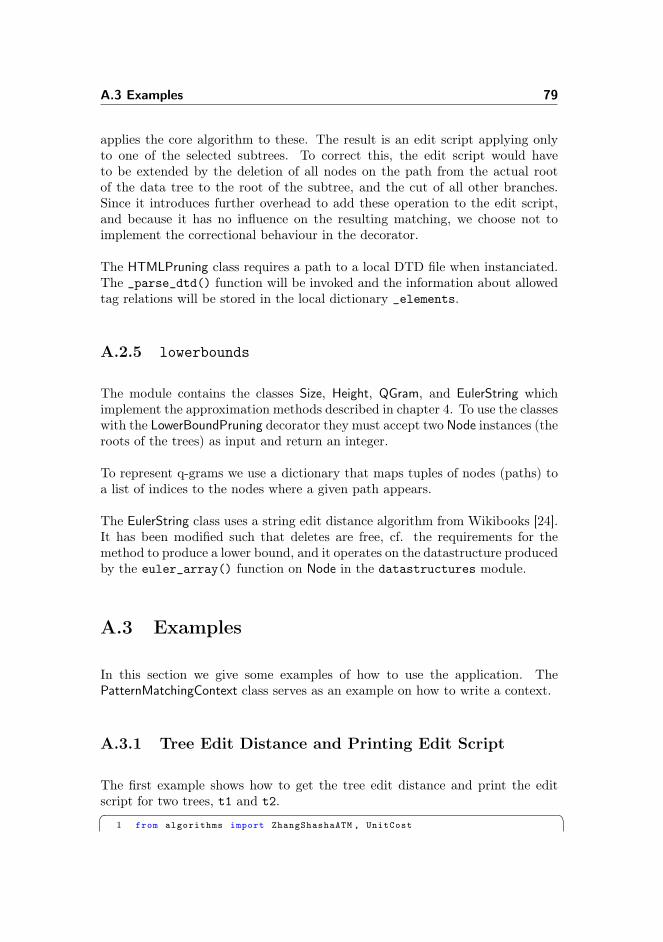
A.3 Examples 79
applies the core algorithm to these. The result is an edit script applying onlyto one of the selected subtrees. To correct this, the edit script would haveto be extended by the deletion of all nodes on the path from the actual rootof the data tree to the root of the subtree, and the cut of all other branches.Since it introduces further overhead to add these operation to the edit script,and because it has no influence on the resulting matching, we choose not toimplement the correctional behaviour in the decorator.
The HTMLPruning class requires a path to a local DTD file when instanciated.The _parse_dtd() function will be invoked and the information about allowedtag relations will be stored in the local dictionary _elements.
A.2.5 lowerbounds
The module contains the classes Size, Height, QGram, and EulerString whichimplement the approximation methods described in chapter 4. To use the classeswith the LowerBoundPruning decorator they must accept two Node instances (theroots of the trees) as input and return an integer.
To represent q-grams we use a dictionary that maps tuples of nodes (paths) toa list of indices to the nodes where a given path appears.
The EulerString class uses a string edit distance algorithm from Wikibooks [24].It has been modified such that deletes are free, cf. the requirements for themethod to produce a lower bound, and it operates on the datastructure producedby the euler_array() function on Node in the datastructures module.
A.3 Examples
In this section we give some examples of how to use the application. ThePatternMatchingContext class serves as an example on how to write a context.
A.3.1 Tree Edit Distance and Printing Edit Script
The first example shows how to get the tree edit distance and print the editscript for two trees, t1 and t2.� �
1 from algorithms import ZhangShashaATM , UnitCost
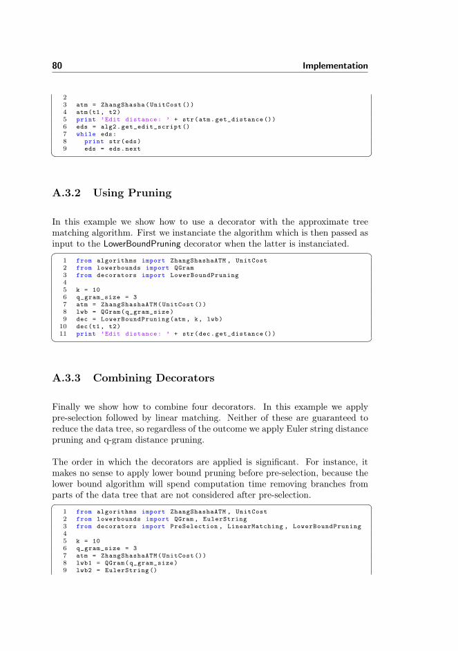
80 Implementation
23 atm = ZhangShasha(UnitCost ())4 atm(t1, t2)5 print ’Edit distance: ’ + str(atm.get_distance ())6 eds = alg2.get_edit_script ()7 while eds:8 print str(eds)9 eds = eds.next� �
A.3.2 Using Pruning
In this example we show how to use a decorator with the approximate treematching algorithm. First we instanciate the algorithm which is then passed asinput to the LowerBoundPruning decorator when the latter is instanciated.� �
1 from algorithms import ZhangShashaATM , UnitCost2 from lowerbounds import QGram3 from decorators import LowerBoundPruning45 k = 106 q_gram_size = 37 atm = ZhangShashaATM(UnitCost ())8 lwb = QGram(q_gram_size)9 dec = LowerBoundPruning(atm , k, lwb)
10 dec(t1, t2)11 print ’Edit distance: ’ + str(dec.get_distance ())� �
A.3.3 Combining Decorators
Finally we show how to combine four decorators. In this example we applypre-selection followed by linear matching. Neither of these are guaranteed toreduce the data tree, so regardless of the outcome we apply Euler string distancepruning and q-gram distance pruning.
The order in which the decorators are applied is significant. For instance, itmakes no sense to apply lower bound pruning before pre-selection, because thelower bound algorithm will spend computation time removing branches fromparts of the data tree that are not considered after pre-selection.� �
1 from algorithms import ZhangShashaATM , UnitCost2 from lowerbounds import QGram , EulerString3 from decorators import PreSelection , LinearMatching , LowerBoundPruning45 k = 106 q_gram_size = 37 atm = ZhangShashaATM(UnitCost ())8 lwb1 = QGram(q_gram_size)9 lwb2 = EulerString ()
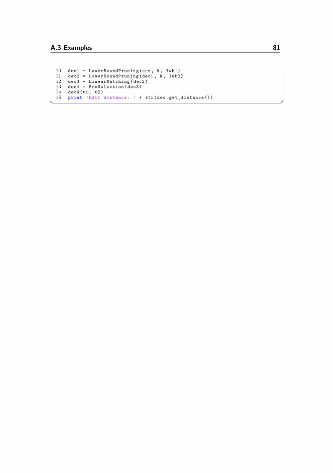
A.3 Examples 81
10 dec1 = LowerBoundPruning(atm , k, lwb1)11 dec2 = LowerBoundPruning(dec1 , k, lwb2)12 dec3 = LinearMatching(dec2)13 dec4 = PreSelection(dec3)14 dec4(t1, t2)15 print ’Edit distance: ’ + str(dec.get_distance ())� �

82 Implementation
Appendix B
Algorithms
B.1 Algorithm for finding Q-grams
Below the algorithm for finding Q-grams is shown. A q-gram profile is a tuple(vx, vy, . . . , vz) of nodes.
The Q-gram algorithm takes a tree T and a value q as input and computes allpaths of length 1, 2, . . . , q for each subtree T (v). The index of the highest nodeis stored in a dictionary qgram (Q-gram profile → [index]) at v. It also usesa dictionary path (length of path → [Q-gram profile]) for each node v to storeall q-grams starting at v. This is to avoid computing a q-gram more than once.The running time of the algorithm is O
(q|T |2
).
B.2 Algorithm for finding Q-samples
The q-sample algorithm takes a tree T and a q value as input and computes asmany disjoint q-grams of size at most q as possible. It is a greedy algorithmin the sense that it will attempt to create the biggest possible q-gram for thecurrent node. Since this may result in one large and several small q-grams it

84 Algorithms
Algorithm 3 Q-gram(T, q)1: for each node vx in T in postorder do2: vx.qgram[(vx)]← [x]3: for each child wy of vx do4: for each q-gram profile p in wy.qgram do5: vx.qgram[p]← vx.qgram[p] ∪ wy.qgram[p]6: if q ≥ 2 then7: vx.qgram[(vx, wy)]← vx.qgram[(vx, wy)] ∪ [x]8: vx.path[2]← vx.path[2] ∪ (vx, wy)9: for i← 2 . . . q do
10: for each path p in wy.path[i] do11: vx.qgram[(vx)⊕ p]← vx.qgram[(vx)⊕ p] ∪ [x]12: vx.path[i+ 1]← vx.path[i+ 1] ∪ (vx)⊕ p
may not be an optimal strategy. It uses the same dictionary qgram as Q-gram.The running time of the algorithm is O
(|T |2
).
Algorithm 4 Q-sample(T, q)1: Let nodes be a FIFO queue of the nodes of T in post order2: while nodes 6= ∅ do3: vx ← nodes.pop()4: k ← q5: s← (vx)6: n← vx7: while n has at least one child and k > 1 do8: Let n be the some child c of n9: Remove c from nodes
10: s← s⊕ (n)11: k ← k − 112: vx.qgram[s]← x13: for each node v in T in postorder do14: for each child w of v do15: for each q-gram profile p in w.qgram do16: v.qgram[p]← v.qgram[p] ∪ w.qgram[p]

Appendix C
Test Case Patterns
C.1 Case 1� �1 <div class="st_content container_24">2 <div class="grid -wrapper clearfix">3 <div class="grid_24 panel -region region -bottom">4 <div class="panel -pane">5 <div class="content">6 <div class="section">7 <section >8 <div class="grid_5 panel -region d">9 <div class="module block -league -table">
10 <h2 class="section -sub -header section -sub -header -style3">
11 </h2>12 <table>13 <tbody >14 <tr>15 <td class="text -b last">16 <a class="black -nl">17 <img src="" />18 </a>19 </td>20 </tr>21 <tr>22 <td class="text -b last">23 <a class="black -nl"></a>24 </td>25 </tr>26 <tr>27 <td class="text -b last">28 <a class="black -nl">
86 Test Case Patterns
29 <img src="" />30 </a>31 </td>32 </tr>33 <tr>34 <td class="text -b last">35 <a class="black -nl">36 <img src="" />37 </a>38 </td>39 </tr>40 <tr>41 <td class="text -b last">42 <a class="black -nl">43 <img src="" />44 </a>45 </td>46 </tr>47 <tr>48 <td class="text -b last">49 <a class="black -nl">50 <img src="" />51 </a>52 </td>53 </tr>54 <tr>55 <td class="text -b last">56 <a class="black -nl">57 <img src="" />58 </a>59 </td>60 </tr>61 <tr>62 <td class="text -b last">63 <a class="black -nl">64 <img src="" />65 </a>66 </td>67 </tr>68 <tr>69 <td class="text -b last">70 <a class="black -nl">71 <img src="" />72 </a>73 </td>74 </tr>75 <tr>76 <td class="text -b last">77 <a class="black -nl">78 <img src="" />79 </a>80 </td>81 </tr>82 <tr>83 <td class="text -b last">84 <a class="black -nl">85 <img src="" />86 </a>87 </td>88 </tr>89 <tr>90 <td class="text -b last">91 <a class="black -nl">92 <img src="" />93 </a>

C.2 Case 2 87
94 </td>95 </tr>96 </tbody >97 </table >98 </div>99 </div>
100 </section >101 </div>102 </div>103 </div>104 </div>105 </div>106 </div>� �C.2 Case 2� �
1 <table>2 <tbody >3 <tr>4 <td class="text -b last">5 <a class="black -nl">6 <img src="" />7 </a>8 </td>9 </tr>
10 <tr>11 <td class="text -b last">12 <a class="black -nl">13 </a>14 </td>15 </tr>16 <tr>17 <td class="text -b last">18 <a class="black -nl">19 <img src="" />20 </a>21 </td>22 </tr>23 <tr>24 <td class="text -b last">25 <a class="black -nl">26 <img src="" />27 </a>28 </td>29 </tr>30 <tr>31 <td class="text -b last">32 <a class="black -nl">33 <img src="" />34 </a>35 </td>36 </tr>37 <tr>38 <td class="text -b last">39 <a class="black -nl">40 <img src="" />41 </a>42 </td>43 </tr>
88 Test Case Patterns
44 <tr>45 <td class="text -b last">46 <a class="black -nl">47 <img src="" />48 </a>49 </td>50 </tr>51 <tr>52 <td class="text -b last">53 <a class="black -nl">54 <img src="" />55 </a>56 </td>57 </tr>58 <tr>59 <td class="text -b last">60 <a class="black -nl">61 <img src="" />62 </a>63 </td>64 </tr>65 <tr>66 <td class="text -b last">67 <a class="black -nl">68 <img src="" />69 </a>70 </td>71 </tr>72 <tr>73 <td class="text -b last">74 <a class="black -nl">75 <img src="" />76 </a>77 </td>78 </tr>79 <tr>80 <td class="text -b last">81 <a class="black -nl">82 <img src="" />83 </a>84 </td>85 </tr>86 </tbody >87 </table >� �
C.3 Case 3� �1 <body class="html front not -logged -in one -sidebar sidebar -second">2 <div id="page -wrapper">3 <div id="page" class="clearfix">4 <section id="zones -content" class="clearfix">5 <div id="content -outer -wrapper" class="clearfix">6 <div id="content -container" class="clearfix container -12 zone
-dynamic zone -content zone content -zone">7 <div id="region -content" class="region region -content
content -region grid -8 even">8 <div id="block -system -main" class="block block -system
block -without -title odd first">9 <div class="block -inner clearfix">
C.4 Case 4 89
10 <div class="content">11 <div class="view -Forside view -id -Forside view -
display -id-toparticles view -dom -id -1">12 <div class="view -content">13 <div class="frontpage -standalone">14 <aside class="illustration">15 <div class="frontpage -standalone -image">16 <img src="" alt="" />17 </div>18 </aside >19 <section >20 <div class="frontpage -standalone -node -title
">21 <h1 class="node -title">22 <a>23 </a>24 </h1>25 </div>26 <div class="frontpage -standalone -teaser">27 <p>28 <a>29 </a>30 </p>31 </div>32 <div class="article -equipment">33 <div class="post -date">34 </div>35 </div>36 </section >37 </div>38 </div>39 </div>40 </div>41 </div>42 </div>43 </div>44 </div>45 </div>46 </section >47 </div>48 </div>49 </body>� �
C.4 Case 4� �1 <div class="block -inner clearfix">2 <div class="content">3 <div class="view -Forside view -id -Forside view -display -id -
toparticles view -dom -id -1">4 <div class="view -content">5 <div class="frontpage -standalone">6 <aside class="illustration">7 <div class="frontpage -standalone -image">8 <img src="" alt="" />9 </div>
10 </aside >11 <section >12 <div class="frontpage -standalone -node -title">13 <h1 class="node -title">
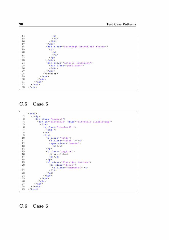
90 Test Case Patterns
14 <a>15 </a>16 </h1>17 </div>18 <div class="frontpage -standalone -teaser">19 <p>20 <a>21 </a>22 </p>23 </div>24 <div class="article -equipment">25 <div class="post -date">26 </div>27 </div>28 </section >29 </div>30 </div>31 </div>32 </div>33 </div>� �
C.5 Case 5� �1 <html>2 <body>3 <div class="content">4 <div id="siteTable" class="sitetable linklisting">5 <div>6 <a class="thumbnail ">7 <img />8 </a>9 <div>
10 <p class="title">11 <a class="title "></a>12 <span class="domain">13 <a></a>14 </p>15 <p class="tagline">16 <time></time>17 <a></a>18 </p>19 <ul class="flat -list buttons">20 <li class="first">21 <a class="comments"></a>22 </li>23 </ul>24 </div>25 </div>26 </div>27 </div>28 </body>29 </html>� �
C.6 Case 6
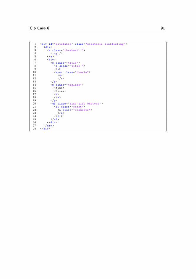
C.6 Case 6 91
� �1 <div id="siteTable" class="sitetable linklisting">2 <div>3 <a class="thumbnail ">4 <img />5 </a>6 <div>7 <p class="title">8 <a class="title ">9 </a>
10 <span class="domain">11 <a>12 </a>13 </p>14 <p class="tagline">15 <time>16 </time>17 <a>18 </a>19 </p>20 <ul class="flat -list buttons">21 <li class="first">22 <a class="comments">23 </a>24 </li>25 </ul>26 </div>27 </div>28 </div>� �

92 Test Case Patterns


![Web Scraping with PHP - php[architect]Web Scraping with PHP, 2nd Ed. III 1. Introduction 1 Intended Audience 1 How to Read This Book 2 Web Scraping Defined 2 Applications of Web Scraping](https://img.dokumen.tips/doc/110x75/5f8efea7104d3f44e5247b03/web-scraping-with-php-phparchitect-web-scraping-with-php-2nd-ed-iii-1-introduction.jpg)