ALGORITHM TYPES Divide and Conquer, Dynamic Programming, Backtracking, and Greedy. Note the general strategy from the examples. The classification is neither

ALGORITHM TYPES

• Divide and Conquer, Dynamic Programming, Backtracking, and Greedy.

• Note the general strategy from the examples.

• The classification is neither exhaustive (there may be more) nor mutually exclusive (one may combine).

Sep'17, 2014 (C) Debasis Mitra

GREEDY Approach: Scheduling problem – Minimize Sum-of-FT

Problem 1

• Input: set of (job-id, duration) pairs,– e.g. (j1, 15), (j2, 8), (j3, 3), (j4, 10)

• Objective function: Sum over Finish Time of all jobs:– in above order, it is 15+23+26+36=100

• Output: Best schedule, for least value of Obj. Func.

• How many possibilities to try?• (j1, j2, j3, j4), (j1, j2, j4, j3), (j1, j3, j2, j4), …

• 4 possibilities for the first position, then 3 for second, 2 for the third, and the only left job goes to the last => 4.3.2.1 = 4!

• n! , for n jobs, if you try all possibilities


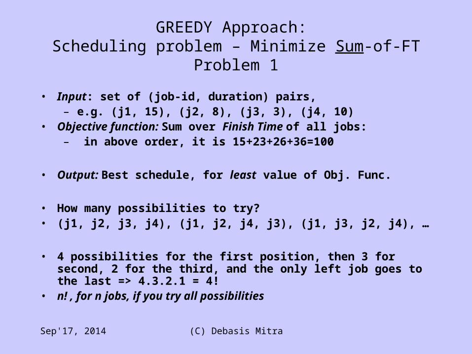
GREEDY Approach: Scheduling problem – Minimize Sum-of-FT

• Input: list of (job-id, duration) pairs,– e.g. (j1, 15), (j2, 8), (j3, 3), (j4, 10)

• Objective function: Sum over Finish Time of all jobs:– in above order, it is 15+23+26+36=100

• Output: Best schedule, for least value of Obj. Func.

• What do you think the best order should be?• Note: durations of tasks are getting added multiple times:

– 15 + (15+8) + ((15+8) + 3) + (((15+8) +3) +10) = 15x4 + 8x3 +3x2 +1x10

• Yes, the best order is shortest-job-first!

• Greedy schedule: j3, j2, j4, j1. – Aggregate FT=3+11+21+36=71 [Let the lower values get added more

times: shortest job first]– This happens to be the best schedule: Optimum

• Complexity: Sort first: O(n log n), then place: (n), – Total: O(n log n)


MULTI-PROCESSOR SCHEDULING (Aggregate FT)Problem 2

• Input: set of (job-id, duration), & number of processors– e.g. {(j2, 5), (j1, 3), (j5, 11), (j3, 6), (j4, 10), (j8, 18), (j6, 14), (j7, 15), (j9, 20)}, & 3

proc

• Objective Fn.: Aggregate FT (AFT) Output: Least AFT

• Greedy Strategy: Pre-sort jobs from low to high– Then, assign ordered jobs over the processors one by one

• Sort: (j1, 3), (j2, 5), (j3, 6), (j4, 10), (j5, 11), (j6, 14), (j7, 15), (j8, 18), (j9, 20) // O (n log n)

• Schedule next job on an earliest available processor – Complexity for assignment: O(n m) for m processors, dominates over O(n log n)– Do you agree, O(n, m)?


MULTI-PROCESSOR SCHEDULING (Aggregate FT)Problem 2

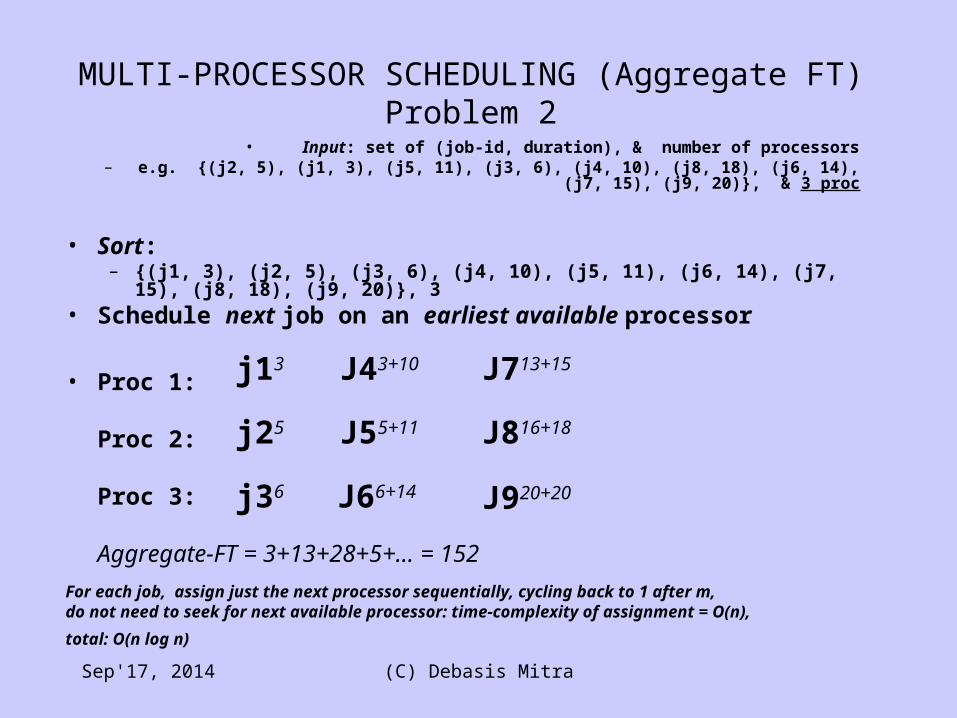
• Input: set of (job-id, duration), & number of processors– e.g. {(j2, 5), (j1, 3), (j5, 11), (j3, 6), (j4, 10), (j8, 18), (j6, 14), (j7, 15), (j9, 20)}, & 3 proc

• Sort: – {(j1, 3), (j2, 5), (j3, 6), (j4, 10), (j5, 11), (j6, 14), (j7, 15), (j8, 18), (j9, 20)}, 3

• Schedule next job on an earliest available processor

• Proc 1:

Proc 2:

Proc 3:

Aggregate-FT = 3+13+28+5+… = 152

For each job, assign just the next processor sequentially, cycling back to 1 after m,do not need to seek for next available processor: time-complexity of assignment = O(n),

total: O(n log n)

j13 J43+10 J713+15

j25 J55+11 J816+18

j36 J66+14 J920+20


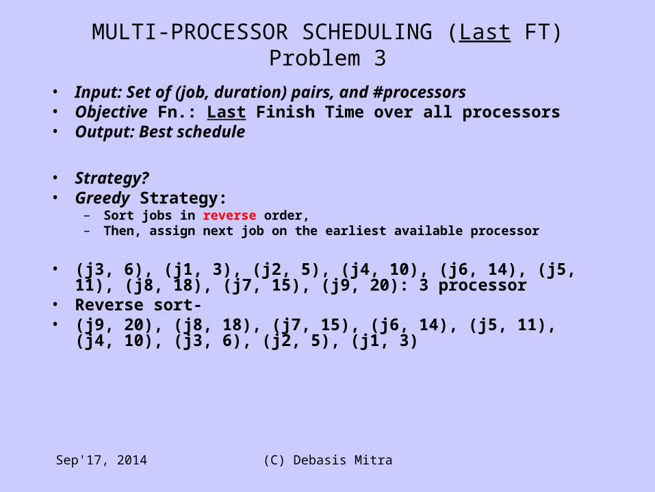
• Input: Set of (job, duration) pairs, and #processors• Objective Fn.: Last Finish Time over all processors• Output: Best schedule

• Strategy?• Greedy Strategy:

– Sort jobs in reverse order, – Then, assign next job on the earliest available processor

• (j3, 6), (j1, 3), (j2, 5), (j4, 10), (j6, 14), (j5, 11), (j8, 18), (j7, 15), (j9, 20): 3 processor

• Reverse sort-• (j9, 20), (j8, 18), (j7, 15), (j6, 14), (j5, 11), (j4, 10), (j3, 6), (j2, 5), (j1, 3)

MULTI-PROCESSOR SCHEDULING (Last FT)Problem 3


• Input: (j3, 6), (j1, 3), (j2, 5), (j4, 10), (j6, 14), (j5, 11), (j8, 18), (j7, 15), (j9, 20): 3 processor• Reverse sort: (j9, 20), (j8, 18), (j7, 15), (j6, 14), (j5, 11), (j4, 10), (j3, 6), (j2, 5), (j1, 3)

• Schedule next job on an earliest available processor

• Proc 1:

Proc 2:

Proc 3:

j920 J420+10 J130+3

j818 J518+11 J329+6

j715 J615+14 J229+5

MULTI-PROCESSOR SCHEDULING (Last FT)


Last-Finish-Time = 35

Complexities?

• Input: Set of (job, duration) pairs, and #processors• Output: Best schedule

• Objective Fn.: Last Finish Time over all jobs

• Greedy Strategy: – Sort jobs in reverse order, – Then, assign next job on the earliest available processor

• Time-complexity• sort: O(n log n)• place: naïve: (nM), with heap over processors: O(n log m)

– O(log m) using HEAP, total O(n logn + n logm) or O(max{n logn, m logm}), for n>>m the first term dominates

• Space complexity?• Space complexity: O(n), for all jobs



• (j3, 6), (j1, 3), (j2, 5), (j4, 10), (j6, 14), (j5, 11), (j8, 18), (j7, 15), (j9, 20): 3 processor

• Greedy Schedule:• Proc 1: j9 - 20, j4 - 30, j1 - 33.• Proc 2: j8 - 18, j5 - 29, j3 - 35,• Proc 3: j7 - 15, j6 - 29, j2 - 34, Greedy Last-FT = 35. • Optimal Schedule:

– Proc1: j2, j5, j8 : 5+11+18=34– Proc 2: j6, j9 : 14+20=34– Proc 3: j1, j3, j4, j7 : 3+6+10+15=34 Optimum Last-FT = 34.

• Greedy algorithm is NOT optimal algorithm here, – but the relative error ≤ [1/3 - 1/(3m)], for m processors– Relative error = (greedyLFT –optimalLFT) / optimalLFT

• An NP-complete problem, • greedy algorithm is polynomial providing approximate solution



HUFFMAN ENCODINGProblem 4

• Problem: formulate a (binary) coding of keys (e.g. character) for a text, – Input: given a set of (character, frequency) pairs (as appears in the

text)

– Objective Function: total number of bits in the text – Output: Variable bit-size encoding, s.t. the objective function is

minimum

• Output Encoding: A binary tree with the characters on leaves (each edge indicating 0 or 1)


i (12)space (13)e (15)

a (10)

t (4)

newline (1)s (3)

0

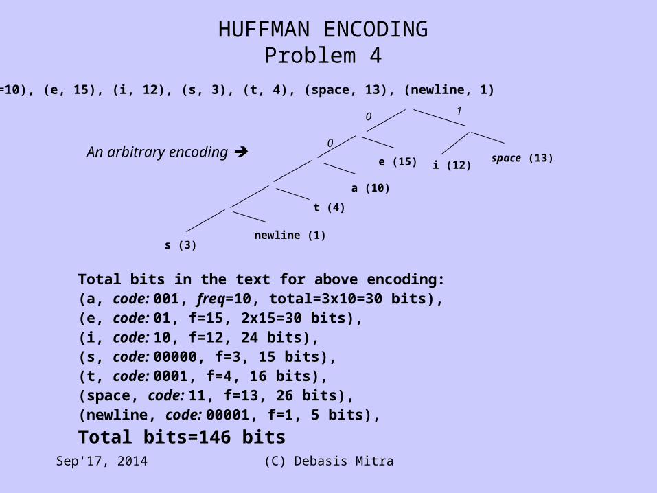
Total bits in the text for above encoding:(a, code: 001, freq=10, total=3x10=30 bits), (e, code: 01, f=15, 2x15=30 bits), (i, code: 10, f=12, 24 bits), (s, code: 00000, f=3, 15 bits), (t, code: 0001, f=4, 16 bits), (space, code: 11, f=13, 26 bits), (newline, code: 00001, f=1, 5 bits),

Total bits=146 bits

i (12)space (13)e (15)

a (10)

t (4)

newline (1)s (3)

0 1

0

HUFFMAN ENCODINGProblem 4

Input: (a, freq=10), (e, 15), (i, 12), (s, 3), (t, 4), (space, 13), (newline, 1)

An arbitrary encoding


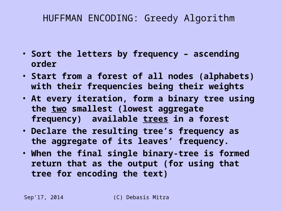
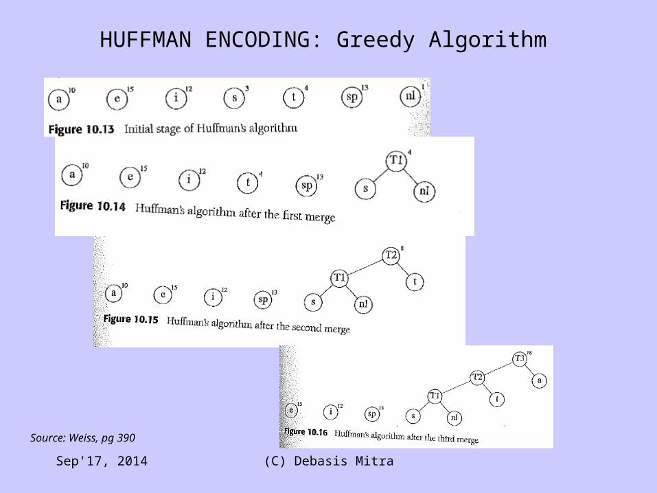
• Sort the letters by frequency – ascending order

• Start from a forest of all nodes (alphabets) with their frequencies being their weights

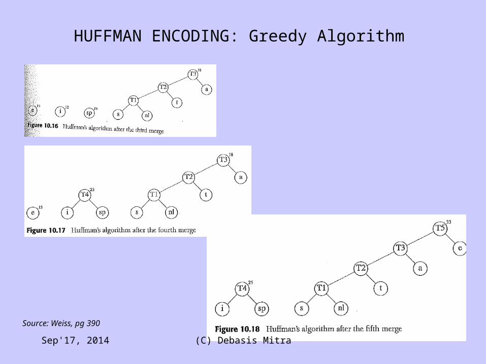
• At every iteration, form a binary tree using the two smallest (lowest aggregate frequency) available trees in a forest

• Declare the resulting tree’s frequency as the aggregate of its leaves’ frequency.

• When the final single binary-tree is formed return that as the output (for using that tree for encoding the text)

HUFFMAN ENCODING: Greedy Algorithm



Source: Weiss, pg 390








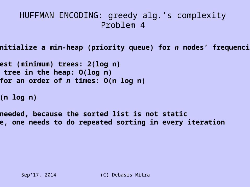
First, initialize a min-heap (priority queue) for n nodes’ frequencies: O(n)

Pick 2 best (minimum) trees: 2(log n)Insert 1 tree in the heap: O(log n)Do that for an order of n times: O(n log n)

Total: O(n log n)

Heap is needed, because the sorted list is not staticOtherwise, one needs to do repeated sorting in every iteration

HUFFMAN ENCODING: greedy alg.’s complexityProblem 4


RATIONAL KNAPSACKProblem 5

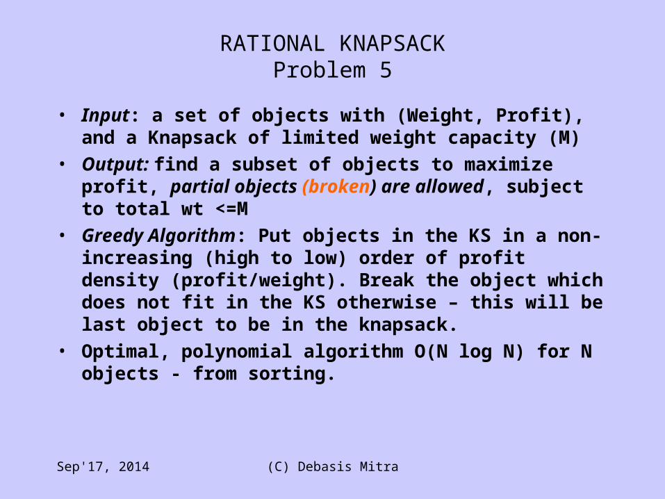
• Input: a set of objects with (Weight, Profit), and a Knapsack of limited weight capacity (M)

• Output: find a subset of objects to maximize profit, partial objects (broken) are allowed, subject to total wt <=M

• Greedy Algorithm: Put objects in the KS in a non-increasing (high to low) order of profit density (profit/weight). Break the object which does not fit in the KS otherwise – this will be last object to be in the knapsack.

• Optimal, polynomial algorithm O(N log N) for N objects - from sorting.


RATIONAL KNAPSACKProblem 5

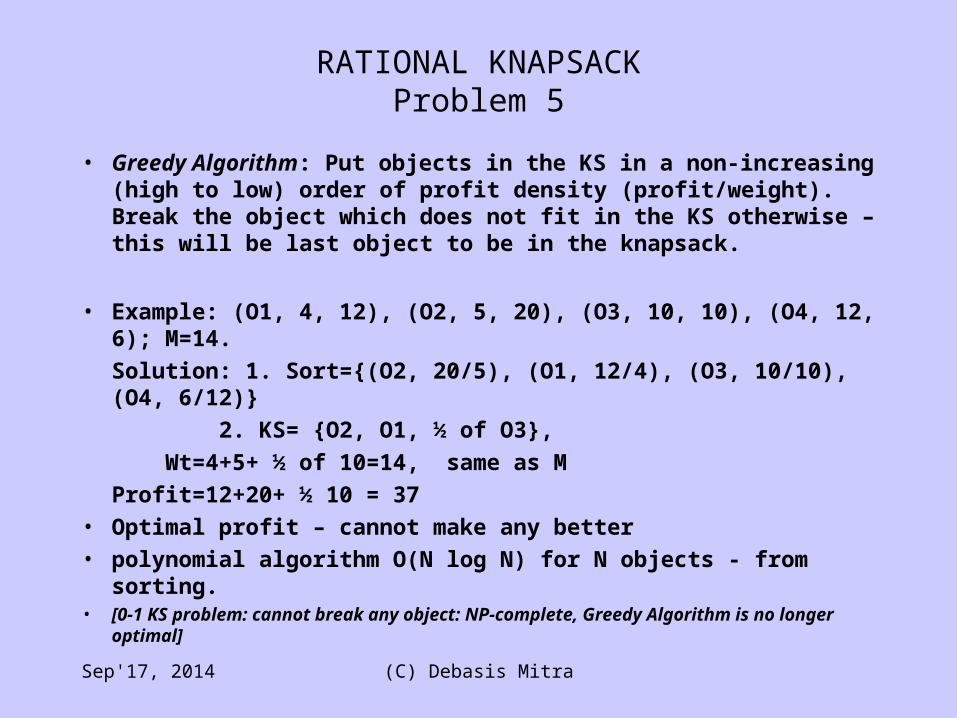
• Greedy Algorithm: Put objects in the KS in a non-increasing (high to low) order of profit density (profit/weight). Break the object which does not fit in the KS otherwise – this will be last object to be in the knapsack.

• Example: (O1, 4, 12), (O2, 5, 20), (O3, 10, 10), (O4, 12, 6); M=14.

Solution: 1. Sort={(O2, 20/5), (O1, 12/4), (O3, 10/10), (O4, 6/12)}

2. KS= {O2, O1, ½ of O3},

Wt=4+5+ ½ of 10=14, same as M

Profit=12+20+ ½ 10 = 37

• Optimal profit – cannot make any better

• polynomial algorithm O(N log N) for N objects - from sorting.• [0-1 KS problem: cannot break any object: NP-complete, Greedy Algorithm is no

longer optimal]


APPROXIMATE BIN PACKING

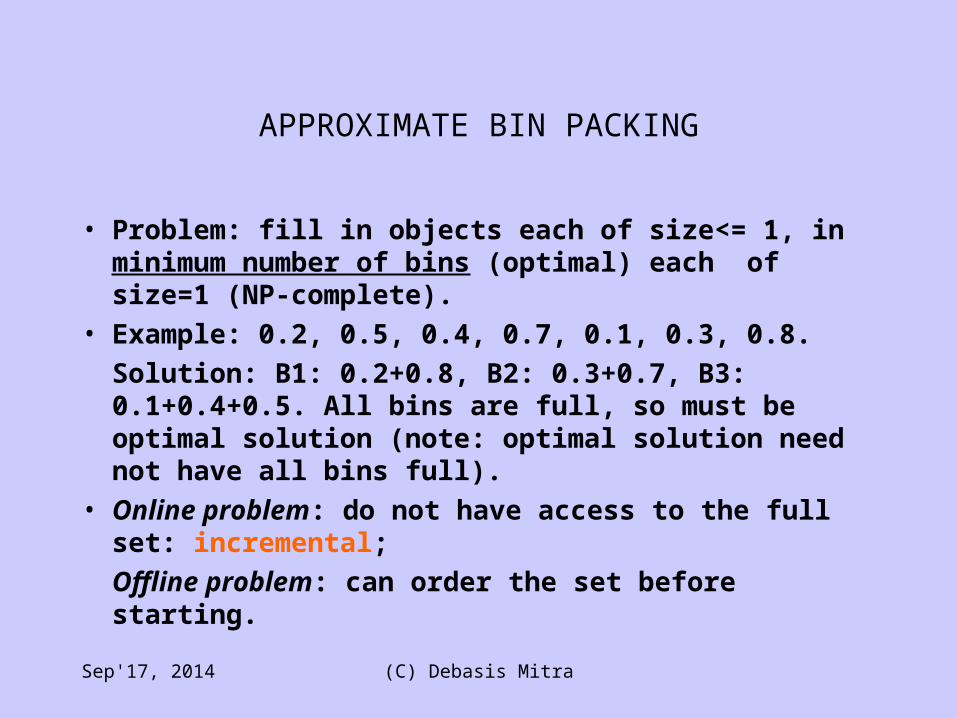
• Problem: fill in objects each of size<= 1, in minimum number of bins (optimal) each of size=1 (NP-complete).

• Example: 0.2, 0.5, 0.4, 0.7, 0.1, 0.3, 0.8.

Solution: B1: 0.2+0.8, B2: 0.3+0.7, B3: 0.1+0.4+0.5. All bins are full, so must be optimal solution (note: optimal solution need not have all bins full).

• Online problem: do not have access to the full set: incremental;

Offline problem: can order the set before starting.


ONLINE BIN PACKING

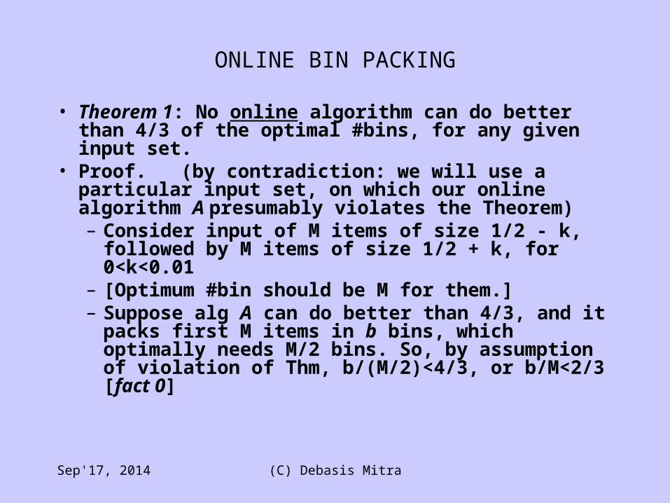
• Theorem 1: No online algorithm can do better than 4/3 of the optimal #bins, for any given input set.

• Proof. (by contradiction: we will use a particular input set, on which our online algorithm A presumably violates the Theorem)– Consider input of M items of size 1/2 - k, followed

by M items of size 1/2 + k, for 0<k<0.01– [Optimum #bin should be M for them.]– Suppose alg A can do better than 4/3, and it packs

first M items in b bins, which optimally needs M/2 bins. So, by assumption of violation of Thm, b/(M/2)<4/3, or b/M<2/3 [fact 0]


ONLINE BIN PACKING

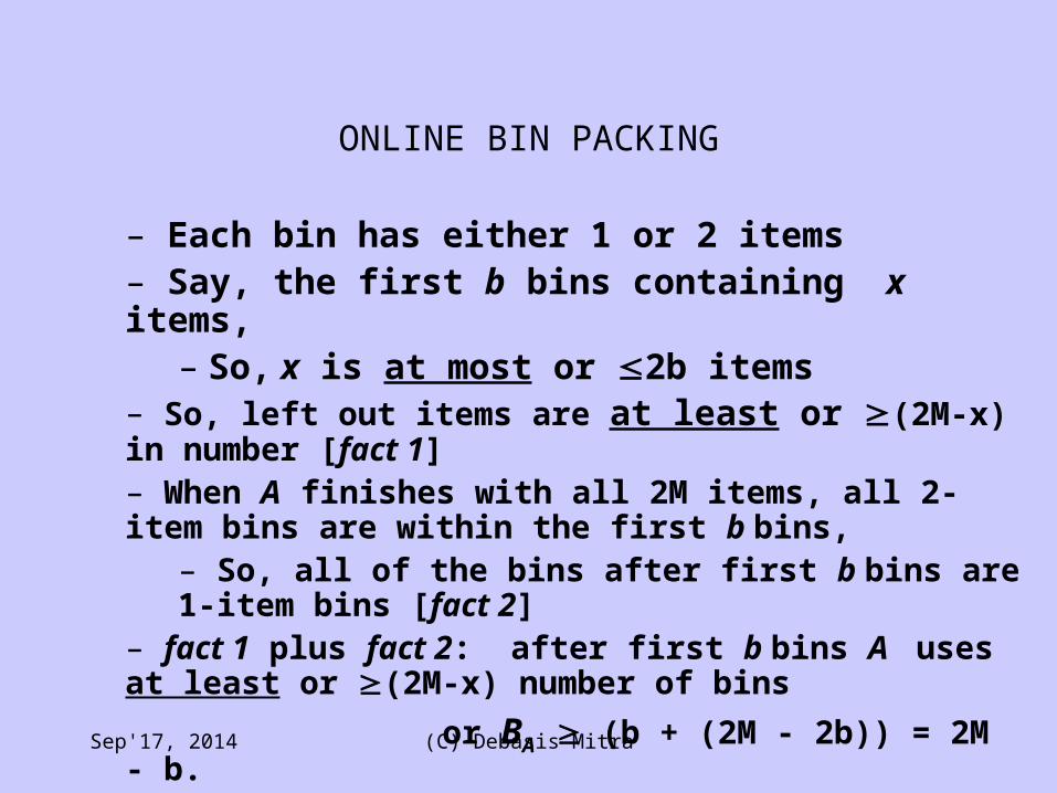
– Each bin has either 1 or 2 items– Say, the first b bins containing x items,

– So, x is at most or 2b items– So, left out items are at least or (2M-x) in number [fact 1]– When A finishes with all 2M items, all 2-item bins are within the first b bins,

– So, all of the bins after first b bins are 1-item bins [fact 2]– fact 1 plus fact 2: after first b bins A uses at least or (2M-x) number of bins

or BA (b + (2M - 2b)) = 2M - b.


ONLINE BIN PACKING

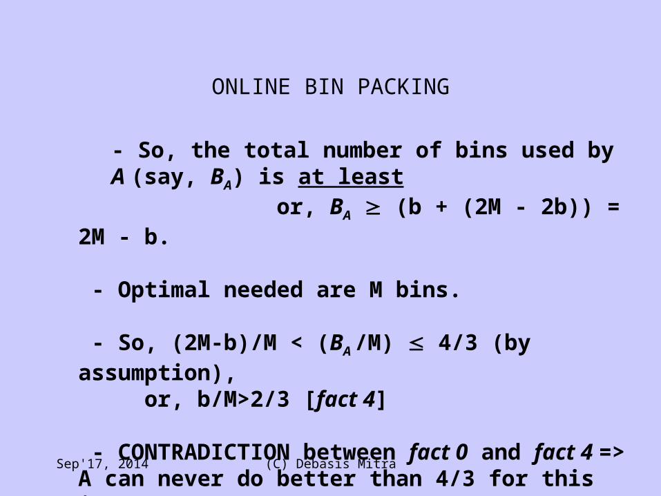
- So, the total number of bins used by A (say, BA) is at least

or, BA (b + (2M - 2b)) = 2M - b.

- Optimal needed are M bins.

- So, (2M-b)/M < (BA /M) 4/3 (by assumption), or, b/M>2/3 [fact 4]

- CONTRADICTION between fact 0 and fact 4 => A can never do better than 4/3 for this input.


NEXT-FIT ONLINE BIN-PACKING

• If the current item fits in the current bin put it there, otherwise move on to the next bin. Linear time with respect to #items - O(n), for n items.

• Example: Weiss Fig 10.21, page 364.• Thm 2: Suppose, M optimum number of bins are

needed for an input. Next-fit never needs more than 2M bins.

• Proof: Content(Bj) + Content(Bj+1) >1, So, Wastage(Bj)

+ Wastage(Bj+1)<2-1, Average wastage<0.5, less than

half space is wasted, so, should not need more than 2M bins.


FIRST-FIT ONLINE BIN-PACKING

• Scan the existing bins, starting from the first bin, to find the place for the next item, if none exists create a new bin. O(N2) naïve, O(NlogN) possible, for N items.

• Obviously cannot need more than 2M bins! Wastes less than Next-fit.

• Thm 3: Never needs more than Ceiling(1.7M).

Proof: too complicated.

• For random (Gaussian) input sequence, it takes 2% more than optimal, observed empirically. Great!


BEST-FIT ONLINE BIN-PACKING

• Scan to find the tightest spot for each item (reduce wastage even further than the previous algorithms), if none exists create a new bin.

• Does not improve over First-Fit in worst case in optimality, but does not take more worst-case time either! Easy to code.


OFFLINE BIN-PACKING

• Create a non-increasing order (larger to smaller) of items first and then apply some of the same algorithms as before.

GOODNESS of FIRST-FIT NON-INCREASING ALGORITHM:• Lemma 1: If M is optimal #of bins, then all items put by the First-

fit in the “extra” (M+1-th bin onwards) bins would be of size 1/3 (in other words, all items of size>1/3, and possibly some items of size 1/3 go into the first M bins).

Proof of Lemma 1. (by contradiction)• Suppose the lemma is not true and the first object that is being put

in the M+1-th bin as the Algorithm is running, is say, si, is of size>1/3.

• Note, none of the first M bins can have more than 2 objects (size of each>1/3). So, they have only one or two objects per bin.


Proof of Lemma 1 continued.• We will prove that the first j bins (0 jM) should have exactly 1 item

each, and next M-j bins have 2 items each (i.e., 1 and 2 item-bins do not mix in the sequence of bins) at the time si is being introduced.

• Suppose contrary to this there is a mix up of sizes and bin# B_x has two items and B_y has 1 item, for 1x<yM.

• The two items from bottom in B_x, say, x1 and x2; it must be x1 y1, where y1 is the only item in B_y

• At the time of entering si, we must have {x1, x2, y1} si, because si is picked up after all the three.

• So, x1+ x2 y1 + si. Hence, if x1 and x2 can go in one bin, then y1 and si also can go in one bin. Thus, first-fit would put si in By, and not in the M+1-th bin. This negates our assumption that single occupied bins could mix with doubly occupied bins in the sequence of bins (over the first M bins) at the moment M+1-th bin is created.

OFFLINE BIN-PACKING


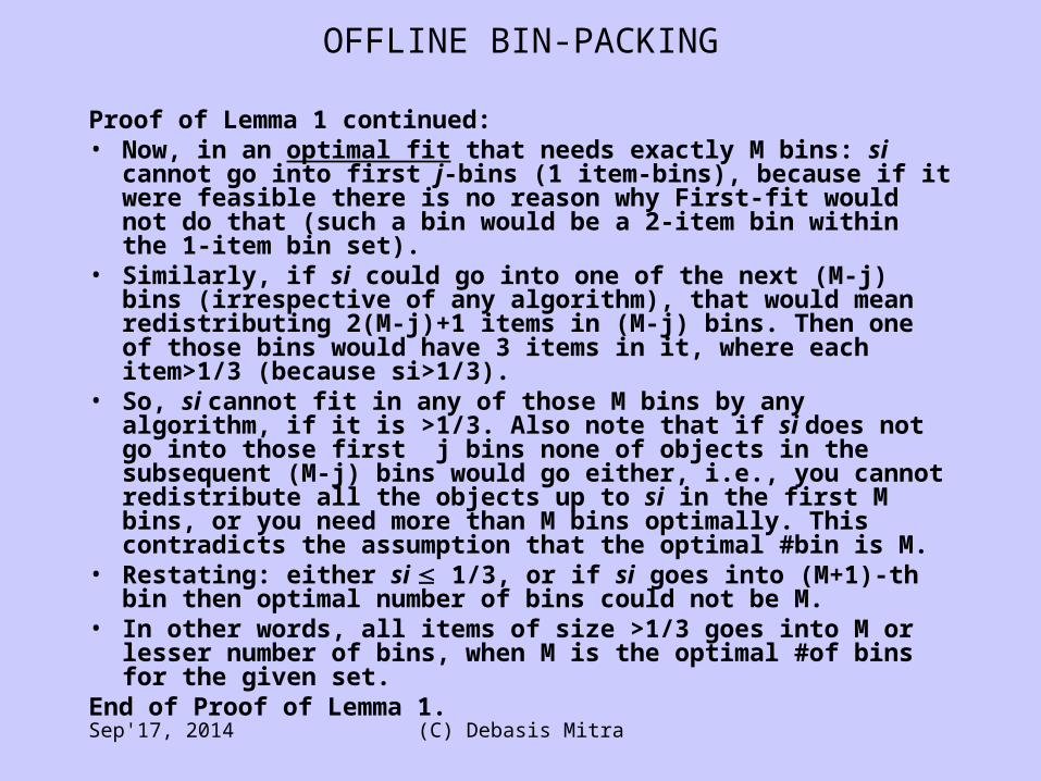
Proof of Lemma 1 continued:• Now, in an optimal fit that needs exactly M bins: si cannot go into

first j-bins (1 item-bins), because if it were feasible there is no reason why First-fit would not do that (such a bin would be a 2-item bin within the 1-item bin set).

• Similarly, if si could go into one of the next (M-j) bins (irrespective of any algorithm), that would mean redistributing 2(M-j)+1 items in (M-j) bins. Then one of those bins would have 3 items in it, where each item>1/3 (because si>1/3).

• So, si cannot fit in any of those M bins by any algorithm, if it is >1/3. Also note that if si does not go into those first j bins none of objects in the subsequent (M-j) bins would go either, i.e., you cannot redistribute all the objects up to si in the first M bins, or you need more than M bins optimally. This contradicts the assumption that the optimal #bin is M.

• Restating: either si 1/3, or if si goes into (M+1)-th bin then optimal number of bins could not be M.

• In other words, all items of size >1/3 goes into M or lesser number of bins, when M is the optimal #of bins for the given set.

End of Proof of Lemma 1.

OFFLINE BIN-PACKING


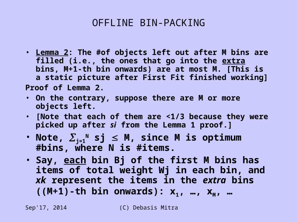
• Lemma 2: The #of objects left out after M bins are filled (i.e., the ones that go into the extra bins, M+1-th bin onwards) are at most M. [This is a static picture after First Fit finished working]

Proof of Lemma 2.• On the contrary, suppose there are M or more objects left.• [Note that each of them are <1/3 because they were picked up

after si from the Lemma 1 proof.]

• Note, j=1N sj M, since M is optimum #bins, where N

is #items.• Say, each bin Bj of the first M bins has items of total

weight Wj in each bin, and xk represent the items in the extra bins ((M+1)-th bin onwards): x1, …, xM, …

OFFLINE BIN-PACKING


OFFLINE BIN-PACKING

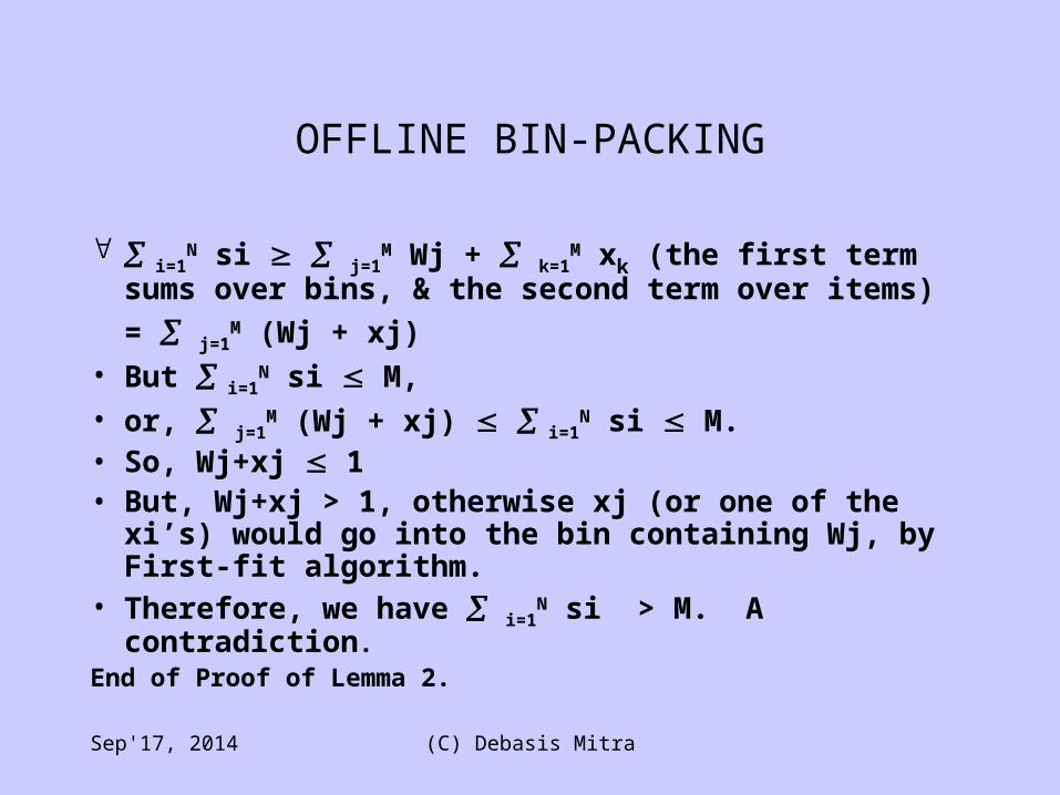
i=1N si j=1

M Wj + k=1M xk (the first term sums over

bins, & the second term over items)

= j=1M (Wj + xj)

• But i=1N si M,

• or, j=1M (Wj + xj) i=1

N si M.• So, Wj+xj 1• But, Wj+xj > 1, otherwise xj (or one of the xi’s) would

go into the bin containing Wj, by First-fit algorithm.• Therefore, we have i=1

N si > M. A contradiction.

End of Proof of Lemma 2.


• Theorem: If M is optimum #bins, then First-fit-offline will not take more than M + (1/3)M #bins.

Proof of Theorem10.4.• #items in “extra” bins is M. They are of size

1/3. So, 3 or more items per those “extra” bins.

• Hence #extra bins itself (1/3)M.• # of non-extra (initial) bins = M. • Total #bins M + (1/3)MEnd of proof.

OFFLINE BIN-PACKING


Documents

ALGORITHM TYPES Divide and Conquer, Dynamic Programming, Backtracking, and Greedy. Note the general strategy from the examples. The classification is neither