Aleksandar Donev - cims.nyu.edudonev/FluctHydro/FluctHydroReview.handout.pdf · Aleksandar Donev Courant Institute, New York University ... 0 is a symmetric positive semide nite mobility

Fluctuating hydrodynamics of complex fluid flows

Aleksandar Donev

Courant Institute, New York University

CECAM WorkshopMolecular Dynamics meets Fluctuating Hydrodynamics

Madrid, May 11th 2015

A. Donev (CIMS) Fluct Hydro 5/2015 1 / 40

Collaborators

Eric Vanden-Eijden, Courant, New York

Pep Espanol, UNED, Madrid

John Bell, Lawrence Berkeley Labs (LBL)

Alejandro Garcia, San Jose State University

Andy Nonaka, LBL

A number of postdocs and graduate students at Courant and LBL.


Diffusion without Hydrodynamics

Uncorrelated Brownian Walkers

Fluctuating hydrodynamics is a coarse-grained description of mass,momentum and energy transport in fluids (gases and liquids).

Consider diffusion of colloidal particles immersed in a viscous liquid;assume the particles are uncorrelated Brownian walkers.

The positions of the N particles Q (t) = q1 (t) , . . . ,qN (t) followthe Ito SDEs

dQ = (2χ)12 dB, (1)

where B(t) is a collection of independent Brownian motions.

We are interested in describing a spatially coarse-grained fluctuatingempirical concentration field,

cξ (r, t) =N∑i=1

δξ (qi (t)− r) , (2)

where δξ is a smoothing kernel with support ∼ ξ that converges to adelta function as ξ → 0.



No Coarse Graining ala Dean

Consider first the limit ξ → 0, which corresponds to no coarsegraining (no loss of information except particle numbering).

Dean obtained an SPDE for c (r, t) =∑δ (qi (t)− r), using

straightforward Ito calculus and properties of the Dirac delta function,

∂tc = χ∇2c + ∇ ·(√

2χcWc

), (3)

where Wc (r, t) denotes a spatio-temporal white-noise vector field.

This is a typical example of a fluctuating hydrodynamics equation,which is deceptively simply, yet extremely subtle from both a physicaland mathematical perspective.

The term√

2χcWc can be thought of as a stochastic mass flux, inaddition to the “deterministic” Fickian flux χ∇c.



What is it useful for?

∂tc = χ∇2c + ∇ ·(√

2χcWc

)(4)

In principle, the Dean equation is not really useful, since it is amathematically ill-defined tautology, a mere rewriting of theoriginal equations for the particles.

The ensemble average c = 〈c〉 follows Fick’s law,

∂t c = ∇ · (χ∇c) = χ∇2c,

which is the law of large numbers (most probable path around whichall paths concentrate) in the limit of large coarse-graining scale ξ.

The central limit theorem describing small Gaussian fluctuationsδc = c − c can be obtained by linearizing,

∂t (δc) = χ∇2 (δc) + ∇ ·(√

2χcWc

).

Note that this equation of linearized fluctuating hydrodynamics ismathematically well-defined.



What is it useful for?

Furthermore, and more surprisingly, the Dean equation correctlypredicts the large deviation action functional for the particle model,and thus correctly gives the probability of observing large deviationsfrom the typical (Fick) behavior.

This suggests the nonlinear fluct. hydro. equation is informative andmaybe useful.

In particular, upon spatially discretizing the (formal) SPDE, theresulting system of SODEs can be seen as a spatial coarse-graining ofthe particle system, which has the right properties.

Numerically solving the discretized Dean equation with weak noisegives results in agreement with all three mathematically well-definedweak-noise limit theorems: LLN, CLT, and LDT.No need to perform linearizations manually, or to discretize stochasticpath integrals directly.


Diffusion with Hydrodynamics

Brownian Dynamics

The Ito equations of Brownian Dynamics (BD) for the (correlated)positions of the N particles Q (t) = q1 (t) , . . . ,qN (t) are

dQ = −M (∂QU) dt + (2kBT M)12 dB + kBT (∂Q ·M) dt, (5)

where B(t) is a collection of independent Brownian motions, U (Q) isa conservative interaction potential.

Here M (Q) 0 is a symmetric positive semidefinite mobility blockmatrix for the collection of particles, and introduces correlationsamong the walkers.

The Fokker-Planck equation (FPE) for the probability density P (Q, t)corresponding to (5) is

∂P

∂t=

∂

∂Q·

M

[∂U

∂QP + (kBT )

∂P

∂Q

], (6)

and is in detailed-balance (i.e., is time reversible) with respect to theGibbs-Boltzmann distribution ∼ exp (−U(Q)/kBT ).



Hydrodynamic Correlations

Let’s start from the (low-density) pairwise approximation

∀ (i , j) : Mij

(qi ,qj

)=

R(qi ,qj

)kBT

=1

kBT

∑k

φk (qi )φk

(qj

),

Here R (r, r′) is a symmetric positive-definite kernel that isdivergence-free, and can be diagonalized in an (infinite dimensional)set of divergence-free basis functions φk (r).

For the Rotne-Prager-Yamakawa tensor mobility,R(r′, r′′) ≡R(r′ − r′′ ≡ r),

R(r) = χ

(

3σ

4r+σ3

2r3

)I +

(3σ

4r− 3σ3

2r3

)r ⊗ r

r2, r > 2σ(

1− 9r

32σ

)I +

(3r

32σ

)r ⊗ r

r2, r ≤ 2σ

(7)

where σ is the radius of the colloidal particles and the diffusioncoefficient χ follows the Stokes-Einstein formula χ = kBT/ (6πησ).



Eulerian Overdamped Dynamics

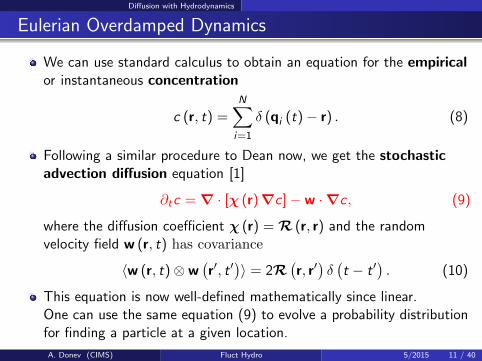
We can use standard calculus to obtain an equation for the empiricalor instantaneous concentration

c (r, t) =N∑i=1

δ (qi (t)− r) . (8)

Following a similar procedure to Dean now, we get the stochasticadvection diffusion equation [1]

∂tc = ∇ · [χ (r)∇c]−w ·∇c, (9)

where the diffusion coefficient χ (r) = R (r, r) and the randomvelocity field w (r, t) has covariance

〈w (r, t)⊗w(r′, t ′

)〉 = 2R

(r, r′)δ(t − t ′

). (10)

This equation is now well-defined mathematically since linear.One can use the same equation (9) to evolve a probability distributionfor finding a particle at a given location.



Importance of Hydrodynamics

For uncorrelated walkers, Mij = δij (kBT )−1 χI, the noise is verydifferent, ∇ ·

(√2χcWc

).

In both cases (hydrodynamically correlated and uncorrelated walkers)the mean obeys Fick’s law but the fluctuations are completelydifferent.

For uncorrelated walkers, out of equilibrium the fluctuations developvery weak long-ranged correlations.

For hydrodynamically correlated walkers, out of equilibrium thefluctuations exhibit very strong “giant” fluctuations with a power-lawspectrum truncated only by gravity or finite-size effects. These giantfluctuations have been confirmed experimentally.



Particle Interactions

U (Q) =1

2

N∑i ,j=1i 6=j

U2(qi ,qj) (11)

Cranking the crank yields the not-so-useful “DDFT” equation

∂tc(r, t) = −∇ · (w (r, t) c(r, t)) + ∇ · (χ(r)∇c(r, t))

+ (kBT )−1∇ ·(c(r, t)

∫R(r, r′)∇′U2(r′, r′′)c(r′, t)c(r′′, t) dr′dr′′

).

All of the equations of fluctuating hydrodynamics have the samestructure of a generic Langevin equation, including these ones:

∂tc = −M [c(·, t)]δH

δc (·, t)+ (2kBT M [c(·, t)])

12 W(·, t)



Generic Structure of Langevin Equations

Here the coarse-grained Hamiltonian is independent of thedynamics,

H [c (·)] = kBT

∫c (r)

(ln(Λ3c (r)

)− 1)dr

+1

2

∫U2(r, r′)c(r)c(r′) drdr′

But the mobility operator depends on dynamics

(M f (·)) (r) =

∫dr′M

[c(·); r, r′

]f (r′) =

≡

− (kBT )−1 ∇ · (χ(r)c(r)∇f (r)) no hydro

− (kBT )−1 ∇ ·(c(r)

∫R (r, r′) c(r′)∇′f (r′) dr′

)hydro


Fluctuating Hydrodynamics Model

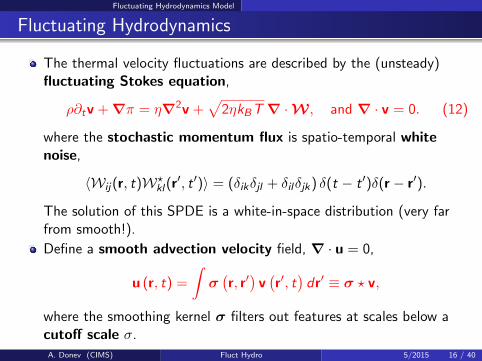
Fluctuating Hydrodynamics

The thermal velocity fluctuations are described by the (unsteady)fluctuating Stokes equation,

ρ∂tv + ∇π = η∇2v +√

2ηkBT ∇ ·W , and ∇ · v = 0. (12)

where the stochastic momentum flux is spatio-temporal whitenoise,

〈Wij(r, t)W?kl(r′, t ′)〉 = (δikδjl + δilδjk) δ(t − t ′)δ(r − r′).

The solution of this SPDE is a white-in-space distribution (very farfrom smooth!).

Define a smooth advection velocity field, ∇ · u = 0,

u (r, t) =

∫σ(r, r′)

v(r′, t)dr′ ≡ σ ? v,

where the smoothing kernel σ filters out features at scales below acutoff scale σ.



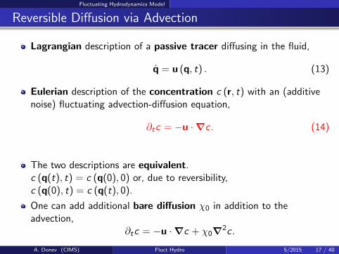
Reversible Diffusion via Advection

Lagrangian description of a passive tracer diffusing in the fluid,

q = u (q, t) . (13)

Eulerian description of the concentration c (r, t) with an (additivenoise) fluctuating advection-diffusion equation,

∂tc = −u ·∇c. (14)

The two descriptions are equivalent.c (q(t), t) = c (q(0), 0) or, due to reversibility,c (q(0), t) = c (q(t), 0).

One can add additional bare diffusion χ0 in addition to theadvection,

∂tc = −u ·∇c + χ0∇2c.



Giant Fluctuations in Diffusive Mixing

Snapshots of concentration in a miscible mixture showing the developmentof a rough diffusive interface due to the effect of thermal fluctuations.These giant fluctuations have been studied experimentally and withhard-disk molecular dynamics [2].



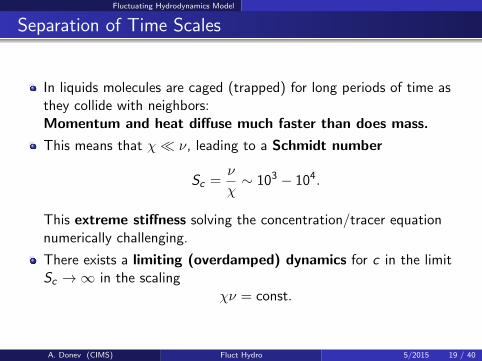
Separation of Time Scales

In liquids molecules are caged (trapped) for long periods of time asthey collide with neighbors:Momentum and heat diffuse much faster than does mass.

This means that χ ν, leading to a Schmidt number

Sc =ν

χ∼ 103 − 104.

This extreme stiffness solving the concentration/tracer equationnumerically challenging.

There exists a limiting (overdamped) dynamics for c in the limitSc →∞ in the scaling

χν = const.



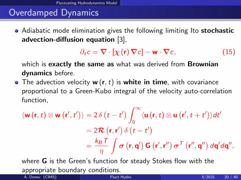
Overdamped Dynamics

Adiabatic mode elimination gives the following limiting Ito stochasticadvection-diffusion equation [3],

∂tc = ∇ · [χ (r)∇c]−w ·∇c, (15)

which is exactly the same as what was derived from Browniandynamics before.The advection velocity w (r, t) is white in time, with covarianceproportional to a Green-Kubo integral of the velocity auto-correlationfunction,

〈w (r, t)⊗w(r′, t ′

)〉 = 2 δ

(t − t ′

) ∫ ∞0〈u (r, t)⊗ u

(r′, t + t ′

)〉dt ′

= 2R(r, r′)δ(t − t ′

)=

kBT

η

∫σ(r,q′

)G(r′, r′′

)σT(r′′,q′′

)dq′dq′′,

where G is the Green’s function for steady Stokes flow with theappropriate boundary conditions.One can obtain the RPY tensor by making the filter σ be a surfacedelta function over a sphere of radius σ.


Coarse-Graining

Coarse Graining

The proper way to interpret fluctuating hydrodynamics is via thetheory of coarse-graining (here I follow Pep Espanol).

The first step is to define a discrete set of relevant variables, whichare mesoscopic observables.


Coarse-Graining

Relevant Variables

How to assign the molecules to the coarse-grained nodes?

If one uses a nearest-node assignment, i.e., Voronoi cells, one getsdivergent Green-Kubo transport coefficients.

Instead, one can use the dual Delaunay cells to constructcoarse-grained variables [4], related to a finite-elementdiscretization of the fluctuating hydrodynamic SPDE.

cµ(Q) =N∑i

δµ(qi ) =N∑i

φµ(qi )

Vµ,

which follow a conservation law since∑

µ Vµcµ = N.

The key assumption is infinite separation of timescales: cµ(Q) ismuch slower than Q itself.


Coarse-Graining

Mori-Zwanzig Formalism

One can use the Mori-Zwanzig formalism with a Markovianassumption (due to separation of timescales) to derive a system ofSDEs for the (discrete) coarse-grained variable c (Q):

dc

dt= −M (c) · ∂F (c)

∂c+ (2kBT M (c))

12 W(t) + (kBT )

∂

∂c·M (c) ,

with the fluctuation-dissipation balance M12

(M

12

)?= M.

Here F (c) is the coarse-grained free energy

Peq(c) =

∫dQ ρeq(Q)δ(c− c(Q)) ∝ exp

−F (c)

kBT

,

which is a purely equilibrium quantity.

The dynamics is captured by the diffusion or mobility SPD matrixM (c), for which one can write generalized Green-Kubo formulas.


Coarse-Graining

Renormalization

If one does this for diffusion-type problems one obtains somethingthat looks very much like a finite-element discretization of thefluctuating hydrodynamic (formal) SPDE.The SPDE is a useful notation to guide the construction ofspatio-temporal discretizations, drawing from years of CFD experience.However, if coarse-graining scale becomes macroscopic, we getFick’s law in the usual local form but with renormalized freeenergy and transport coefficients:

∂tc = χ∇2Π(c) = χ∇ ·(dΠ(c)

dc∇c

),

where Π(c) = c (df /dc)− f is the osmotic pressure, where f (c) isthe thermodynamic thermodynamic equilibrium free-energy.In-between the microscopic and macroscopic lies a whole continuumof scales: The free energy and transport coefficients (mobility)must depend on the coarse-graining scale in nonlinearfluctuating hydrodynamics (but not in linearized fluct. hydro).


Complex Fluid Mixtures

Multiphase Systems: Liquid-Vapor

We will use a diffusive-interface model for describing interfacesbetween two distinct phases such as liquid and vapor of a singlespecies.

Coarse-grained free energy follows the usual square-gradient surfacetension model

F (ρ(r),∇ρ(r),T (r)) =

∫dr

(f (ρ(r),T (r)) +

1

2κ |∇ρ(r)|2

)(16)

The local free energy density f (ρ(r),T (r)) includes the hard-corerepulsions as well as the short-range attractions.

Assume a van der Waals loop for the equation of state,

P (ρ,T ) =nkBT

1− b′n− a′n2, (17)

f = nkBT ln

[ρ

1− b′n

]− a′n2.



Fluctuating Hydrodynamics

∂tρ+∇ · (ρv) = 0 (18)

∂t (ρv) +∇ ·(ρvvT

)+∇ ·Π = ∇ · (σ + Σ) (19)

∂t (ρE ) +∇ · (ρEv + Π · v) = ∇ · (ψ + Ψ) +∇ · ((σ + Σ) · v) , (20)

where the momentum density is g = ρv andthe total local energy density is ρE = 1

2ρv2 + ρe.



Momentum Fluxes

The reversible contribution to the stress tensor is [5]

Π = PI−[(κρ∇2ρ+

1

2κ |∇ρ|2

)I

]− (κ∇ρ⊗∇ρ) + cross term?

Irreversible contribution to the stress is the viscous stress tensor

σ = η(∇v + (∇v)T

)+

(ζ − 2

3η

)(∇ · v) I (21)

Stochastic stress tensor obeys fluctuation-dissipation balance

Σ =√

2ηkBT W +

(√ζkBT

3−√

2ηkBT

3

)Tr(W)

I, (22)

where W = (W + WT )/√

2 is a symmetric white-noise tensor field.



Capillary Waves

Variance of height fluctuations versus wavenumber comparing 2Dsimulations (red circles) and capillary wave theory (CWT) (black solidline).



Spinodal Decomposition

Spinodal decomposition in a near-critical Argon system at ρ = 0.416 g/cc,T = 145.85 K leading to a bicontinuous pattern.



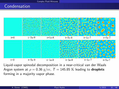
Condensation

Liquid-vapor spinodal decomposition in a near-critical van der WaalsArgon system at ρ = 0.36 g/cc, T = 145.85 K leading to dropletsforming in a majority vapor phase.



Chemically-Reactive Mixtures

The species density equations for a mixture of NS species are given by

∂

∂t(ρs) +∇ · (ρsv + F) = msΩs , (s = 1, . . .NS) (23)

Due to mass conservation ρ =∑

s ρs follows the continuity equation,

∂

∂tρ+∇ · (ρv) = 0. (24)

The mass fluxes take the form, excluding barodiffusion andthermodiffusion,

F = ρW

[χΓ∇x +

√2

nχ

12WF (r, t)

],

where n is the number density, xs is the mole fraction of species s,and W = Diag ws = ρs/ρ contains the mass fractions.



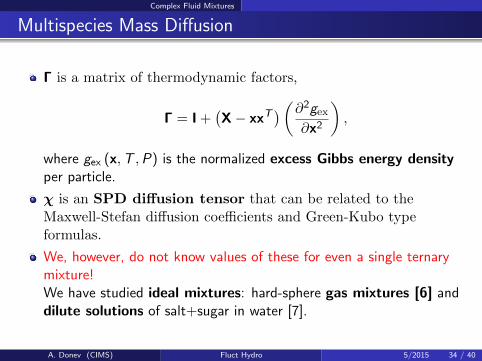
Multispecies Mass Diffusion

Γ is a matrix of thermodynamic factors,

Γ = I +(X− xxT

)(∂2gex∂x2

),

where gex (x,T ,P) is the normalized excess Gibbs energy densityper particle.

χ is an SPD diffusion tensor that can be related to theMaxwell-Stefan diffusion coefficients and Green-Kubo typeformulas.

We, however, do not know values of these for even a single ternarymixture!We have studied ideal mixtures: hard-sphere gas mixtures [6] anddilute solutions of salt+sugar in water [7].



Chemistry

Consider a system with NR elementary reactions with reaction r

Rr :

NS∑s=1

ν+srMs

NS∑s=1

ν−srMs

The stoichiometric coefficients are νsr = ν−sr − ν+sr and mass

conservation requires that∑

s νsrmr = 0.

Define the dimensionless chemical affinity

Ar =∑s

ν+sr µs −

∑s

ν−sr µs ,

where µs = msµs/kBT is the dimensionless chemical potential perparticle.

Also define the thermodynamic driving force

Ar = exp

(∑s

ν+sr µs

)− exp

(∑s

ν−sr µs

)=∏s

eν+sr µs −

∏s

eν−sr µs



Chemistry

The mass production due to chemistry can take one of two forms [8]:

Ωs =∑r

νsr

(P

τrkBT

)Ar (deterministic LMA) (25)

+∑r

νsr

(

2 PτrkBT

ArAr

) 12 Z (r, t) log-mean eq. (LME)(

PτrkBT

∏s e

ν+sr µs) 1

2 Z (r, t) chemical Langevin eq. (CLE)

The LME follows the correct structure of Langevin equations(GENERIC structure of Ottinger/Grmela). Is time-reversible (obeysdetailed balance) at thermodynamic equilibrium wrt to the Einsteindistribution.

The CLE follows from a truncation of the Kramers-Moyal expansionat second order. No true thermodynamic equilibrium since it assumesone-way reactions.

Which one is correct? Neither!A. Donev (CIMS) Fluct Hydro 5/2015 36 / 40


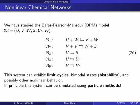
Nonlinear Chemical Networks

We have studied the Baras-Pearson-Mansour (BPM) modelM = (U,V ,W ,S ,Uf ,Vf ),

R1 : U + W V + W

R2 : V + V W + S

R3 : V S (26)

R4 : U Uf

R5 : V Vf

This system can exhibit limit cycles, bimodal states (bistability), andpossibly other nonlinear behavior.In principle this system can be simulated using particle methods!



Turing-like Patterns

Development of an instability in the BPM model with fluctuations (top)and without (bottom) with complete compressible hydrodynamics (not justreaction-diffusion).



Poisson Noise

The reason neither LME nor CLE are correct is that there is noS(P)DE that can correctly describe both the short-time (typical) andlong-time (rare event) behavior of the master equation.

This is related to the fact that the central limit theorem andlarge-deviation theory are not consistent with the same nonlinearS(P)DE.

One must either use the Chemical Master Equation (CME) withSSA/Gillespie (microscopic rather than macroscopic), or

One can use Poisson noise instead of Gaussian noise using tauleaping.This can be thought of as a coarse-graining in time of the originaljump process described by the CME.

Quite generally the appropriateness of assuming Gaussian white noisefor the stochastic fluxes is questionable.



References

A. Donev and E. Vanden-Eijnden.

Dynamic Density Functional Theory with hydrodynamic interactions and fluctuations.J. Chem. Phys., 140(23), 2014.

A. Donev, A. J. Nonaka, Y. Sun, T. G. Fai, A. L. Garcia, and J. B. Bell.

Low Mach Number Fluctuating Hydrodynamics of Diffusively Mixing Fluids.Communications in Applied Mathematics and Computational Science, 9(1):47–105, 2014.

A. Donev, T. G. Fai, and E. Vanden-Eijnden.

A reversible mesoscopic model of diffusion in liquids: from giant fluctuations to Fick’s law.Journal of Statistical Mechanics: Theory and Experiment, 2014(4):P04004, 2014.

P. Espanol and I. Zuniga.

On the definition of discrete hydrodynamic variables.J. Chem. Phys, 131:164106, 2009.

A. Chaudhri, J. B. Bell, A. L. Garcia, and A. Donev.

Modeling multiphase flow using fluctuating hydrodynamics.Phys. Rev. E, 90:033014, 2014.

K. Balakrishnan, A. L. Garcia, A. Donev, and J. B. Bell.

Fluctuating hydrodynamics of multispecies nonreactive mixtures.Phys. Rev. E, 89:013017, 2014.

A. Donev, A. J. Nonaka, A. K. Bhattacharjee, A. L. Garcia, and J. B. Bell.

Low Mach Number Fluctuating Hydrodynamics of Multispecies Liquid Mixtures.Physics of Fluids, 27(3), 2015.

A. K. Bhattacharjee, K. Balakrishnan, A. L. Garcia, J. B. Bell, and A. Donev.

Fluctuating hydrodynamics of multispecies reactive mixtures.Submitted to J. Chem. Phys., ArXiv preprint 1503.07478, 2015.


Documents

Aleksandar Donev - cims.nyu.edudonev/FluctHydro/FluctHydroReview.handout.pdf · Aleksandar Donev Courant Institute, New York University ... 0 is a symmetric positive semide nite mobility