Embed Size (px)
Citation preview

Analysis of Planform Changes using Satellite
Images
A.K.M. Saiful Islam Associate Professor, IWFM, BUET
December 2010 Email: [email protected]
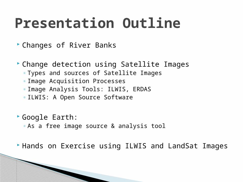
Changes of River Banks
Change detection using Satellite Images◦ Types and sources of Satellite Images◦ Image Acquisition Processes◦ Image Analysis Tools: ILWIS, ERDAS◦ ILWIS: A Open Source Software
Google Earth: ◦ As a free image source & analysis tool
Hands on Exercise using ILWIS and LandSat Images
Presentation Outline
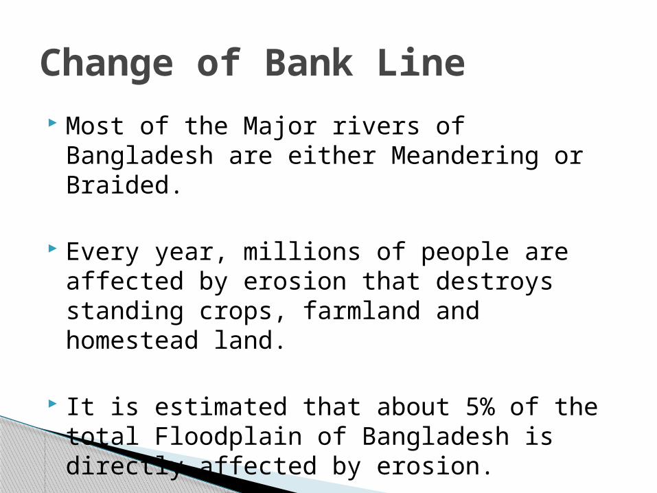
Most of the Major rivers of Bangladesh are either Meandering or Braided.
Every year, millions of people are affected by erosion that destroys standing crops, farmland and homestead land.
It is estimated that about 5% of the total Floodplain of Bangladesh is directly affected by erosion.
Change of Bank Line
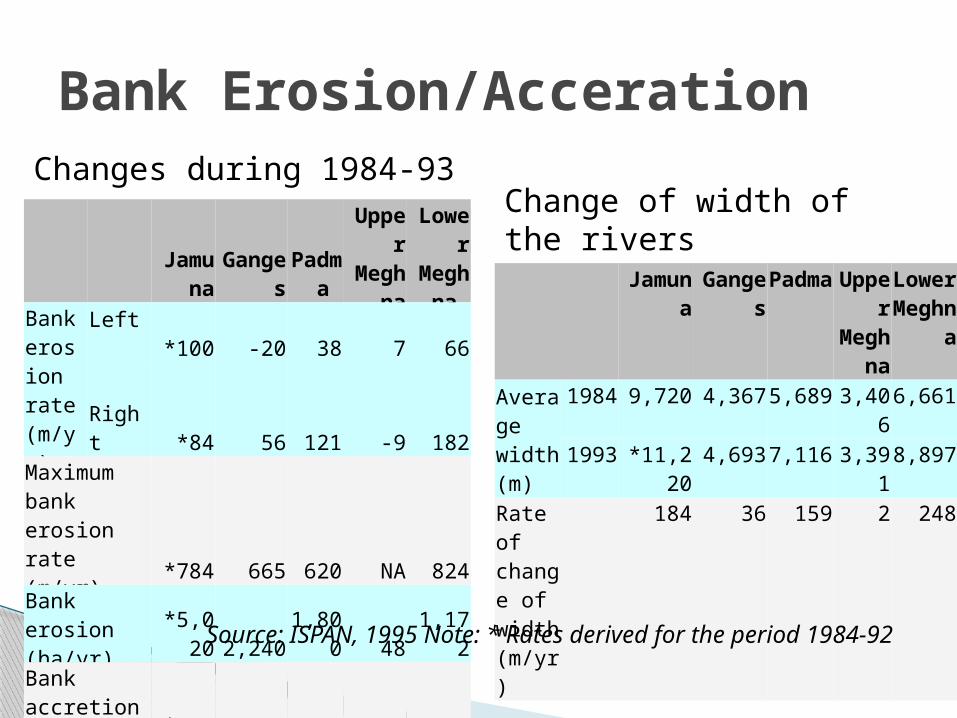
Jamuna Ganges Padma Upper Megh
na
Lower Meghn
aAverage width (m)
1984 9,720 4,367 5,689 3,406 6,661
1993 *11,220 4,693 7,116 3,391 8,897
Rate of change of width (m/yr)
184 36 159 2 248
Changes during 1984-93
Jamun
a GangesPadm
a
Upper Megh
na
Lower Megh
na
Bank erosion rate (m/yr)
Left *100 -20 38 7 66
Right *84 56 121 -9 182
Maximum bank erosion rate (m/yr) *784 665 620 NA 824Bank erosion (ha/yr) *5,020 2,240 1,800 48 1,172
Bank accretion (ha/yr) *890 1,010 233 49 402
Change of width of the rivers
Source: ISPAN, 1995 Note: * Rates derived for the period 1984-92
Bank Erosion/Acceration

Severity of ErosionTeesta River at Sundarganj
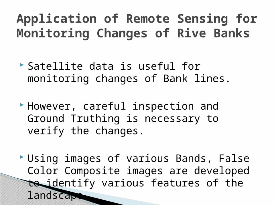
Satellite data is useful for monitoring changes of Bank lines.
However, careful inspection and Ground Truthing is necessary to verify the changes.
Using images of various Bands, False Color Composite images are developed to identify various features of the landscape.
Application of Remote Sensing for Monitoring Changes of Rive Banks
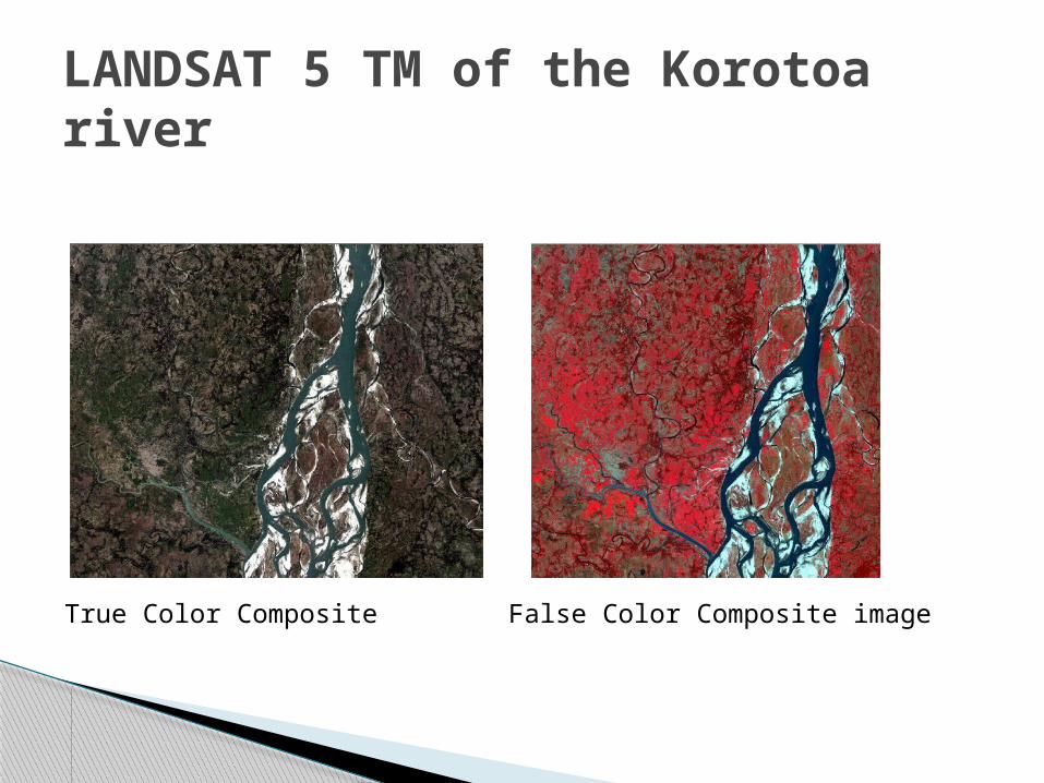
LANDSAT 5 TM of the Korotoa river
True Color Composite False Color Composite image
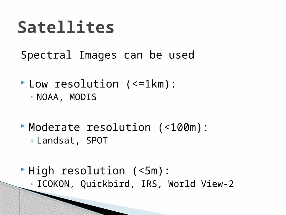
Spectral Images can be used
Low resolution (<=1km): ◦ NOAA, MODIS
Moderate resolution (<100m): ◦ Landsat, SPOT
High resolution (<5m): ◦ ICOKON, Quickbird, IRS, World View-2
Satellites
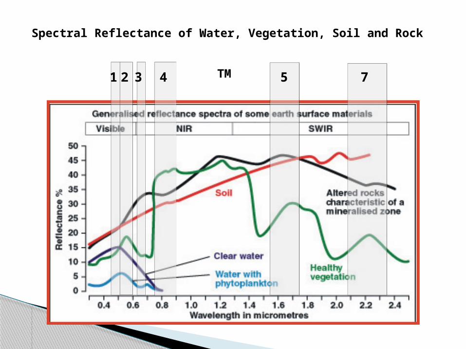
Spectral Reflectance of Water, Vegetation, Soil and Rock
12 3 4 5 7TM
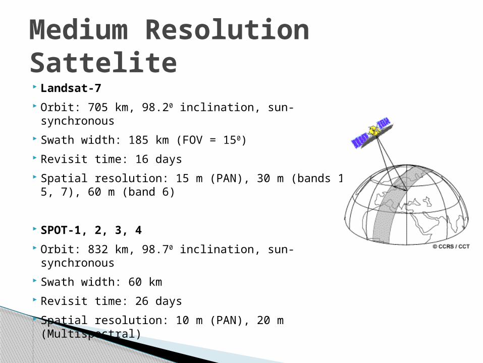
Medium Resolution Sattelite
Landsat-7
Orbit: 705 km, 98.20 inclination, sun-synchronous
Swath width: 185 km (FOV = 150)
Revisit time: 16 days
Spatial resolution: 15 m (PAN), 30 m (bands 1-5, 7), 60 m (band 6)
SPOT-1, 2, 3, 4
Orbit: 832 km, 98.70 inclination, sun-synchronous
Swath width: 60 km
Revisit time: 26 days
Spatial resolution: 10 m (PAN), 20 m (Multispectral)
High Resolution Satellites
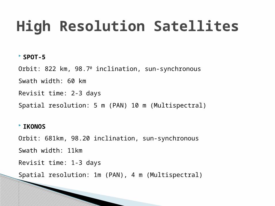
SPOT-5
Orbit: 822 km, 98.70 inclination, sun-synchronous
Swath width: 60 km
Revisit time: 2-3 days
Spatial resolution: 5 m (PAN) 10 m (Multispectral)
IKONOS
Orbit: 681km, 98.20 inclination, sun-synchronous
Swath width: 11km
Revisit time: 1-3 days
Spatial resolution: 1m (PAN), 4 m (Multispectral)

QuickBird WorldView-1 WorldView-2
23 m 6.5 m 6.5 m
QuickBird WorldView-1 WorldView-2
Panchromatic (B&W)
450 - 900 nm 400 - 900 nm 450 - 800 nm
Multispectral:
Coastal Blue 400 - 450 nm
Blue 450 - 520 nm 450 - 510 nm
Green 520 - 600 nm 510 - 580 nm
Yellow 585 - 625 nm
Red 630 - 690 nm 630 - 690 nm
Red Edge 705 - 745 nm
Near-IR 1 760 - 900 nm 770 - 895 nm
Near-IR 2 860 - 1040 nm
High Resolution Satellites
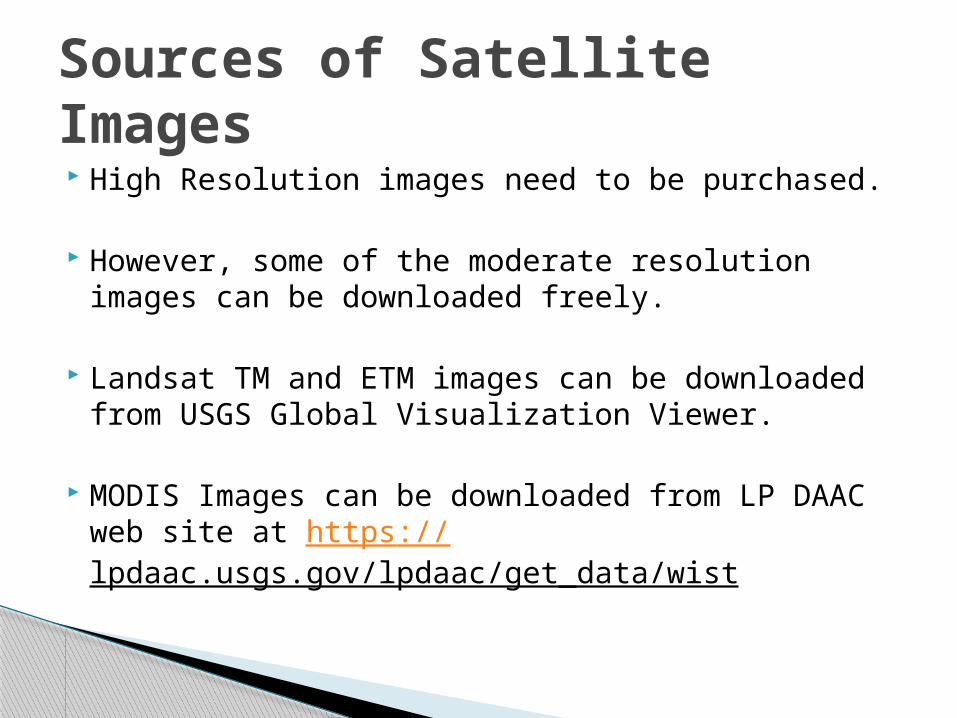
High Resolution images need to be purchased.
However, some of the moderate resolution images can be downloaded freely.
Landsat TM and ETM images can be downloaded from USGS Global Visualization Viewer.
MODIS Images can be downloaded from LP DAAC web site at https://lpdaac.usgs.gov/lpdaac/get_data/wist
Sources of Satellite Images
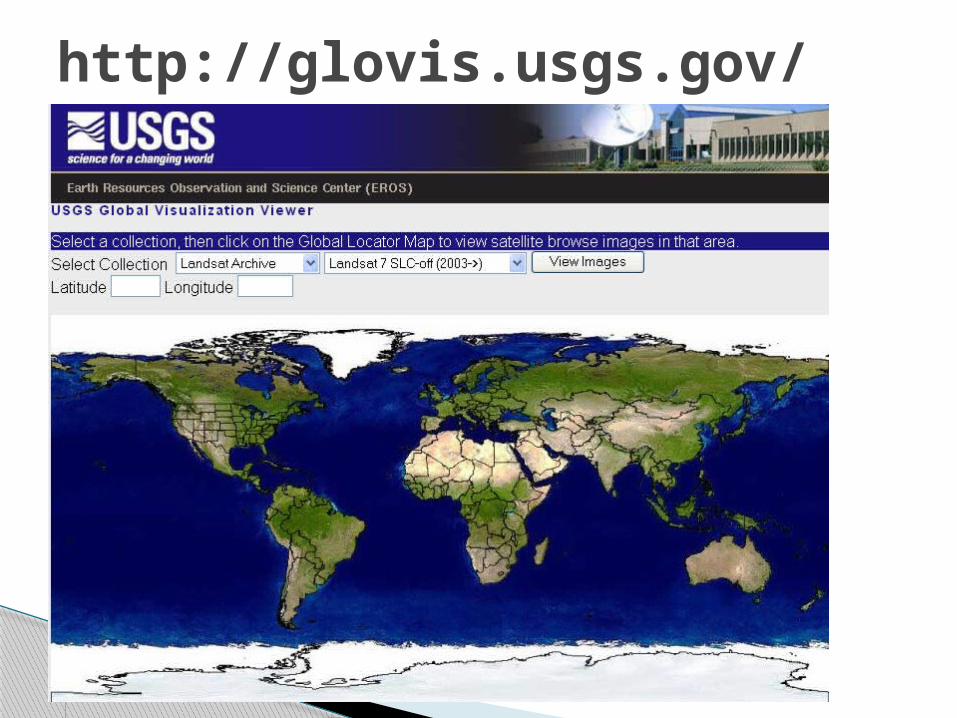
http://glovis.usgs.gov/
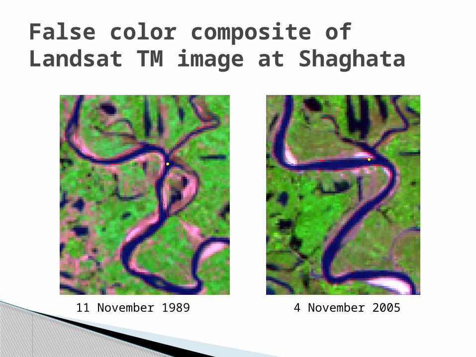
False color composite of Landsat TM image at Shaghata
11 November 1989 4 November 2005
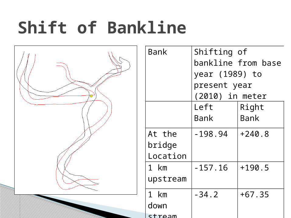
Bank Shifting of bankline from base year (1989) to present year (2010) in meterLeft Bank Right Bank
At the bridge Location
-198.94 +240.8
1 km upstream
-157.16 +190.5
1 km down stream
-34.2 +67.35
Shift of Bankline
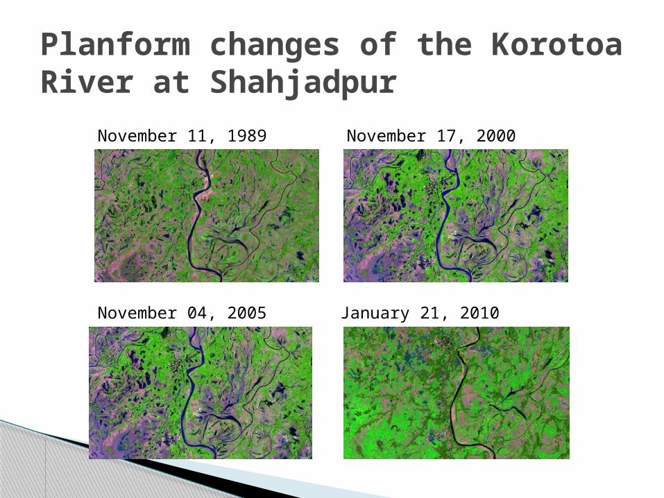
Planform changes of the Korotoa River at Shahjadpur
November 11, 1989 November 17, 2000
November 04, 2005 January 21, 2010
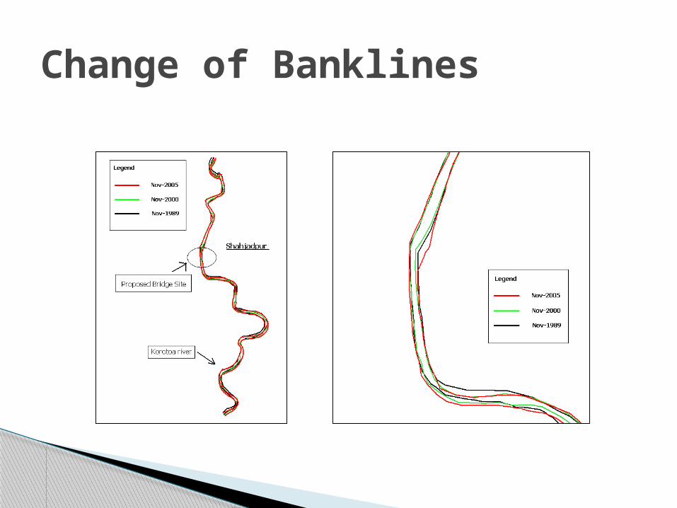
Change of Banklines
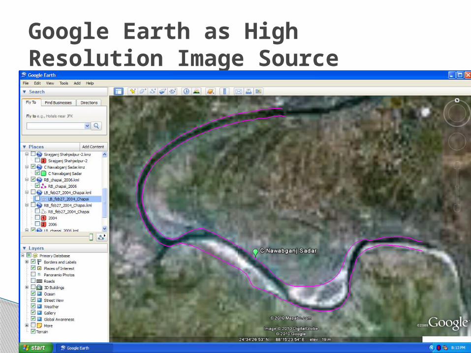
Google Earth as High Resolution Image Source
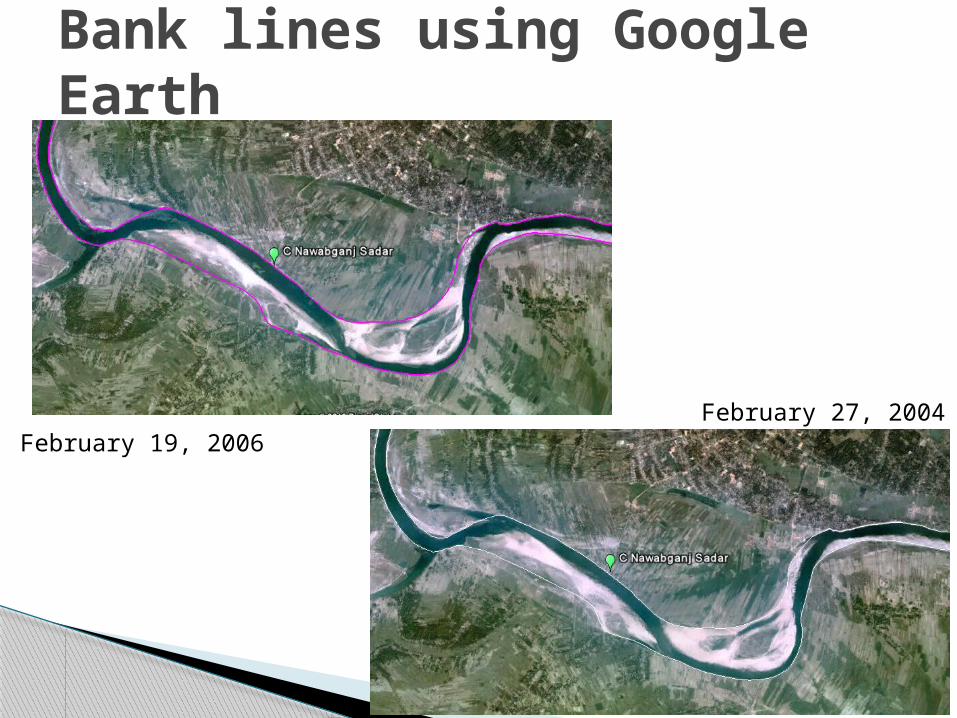
Bank lines using Google Earth
February 19, 2006February 27, 2004

Shifting of bank line from base year (2004) to present (m)
At the bridge Location
-1.9 16.2
1 km upstream -1.3 15.3
1 km down stream
-2.9 15.3
Shift of Bank lines

Hands on Exercise on Planform changes of River
using Satellite Images
A.K.M. Saiful IslamIWFM, BUET
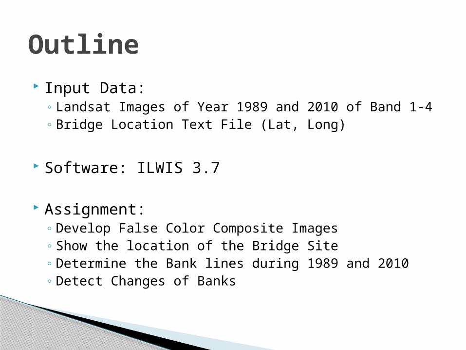
Input Data: ◦ Landsat Images of Year 1989 and 2010 of Band 1-4◦ Bridge Location Text File (Lat, Long)
Software: ILWIS 3.7
Assignment: ◦ Develop False Color Composite Images ◦ Show the location of the Bridge Site◦ Determine the Bank lines during 1989 and 2010◦ Detect Changes of Banks
Outline
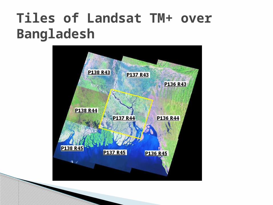
Tiles of Landsat TM+ over Bangladesh
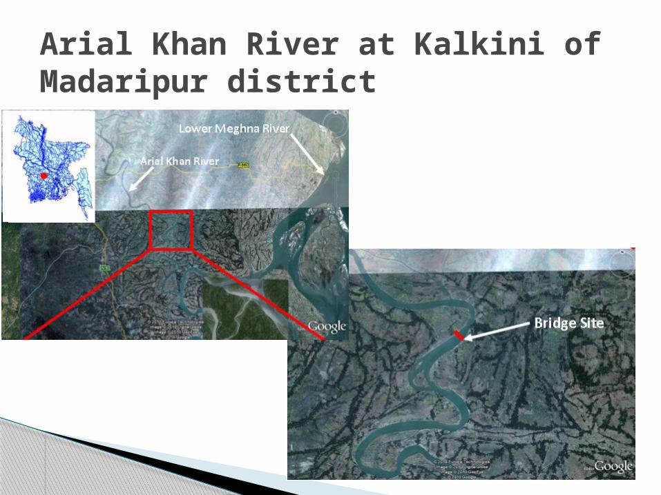
Arial Khan River at Kalkini of Madaripur district
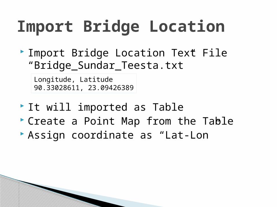
Import Bridge Location Text File “Bridge_Sundar_Teesta.txt”
It will imported as Table Create a Point Map from the Table Assign coordinate as “Lat-Lon”
Import Bridge Location
Longitude, Latitude90.33028611, 23.09426389

Use Import Wizard, Select Text files, Press Next Button
Importing Bridge Locations
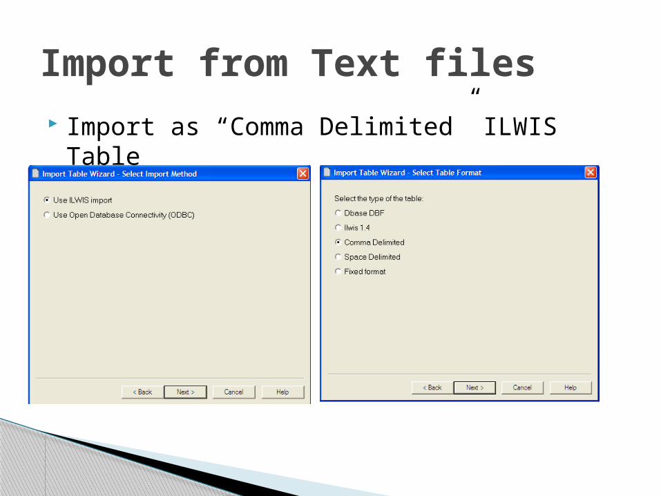
Import as “Comma Delimited” ILWIS Table
Import from Text files
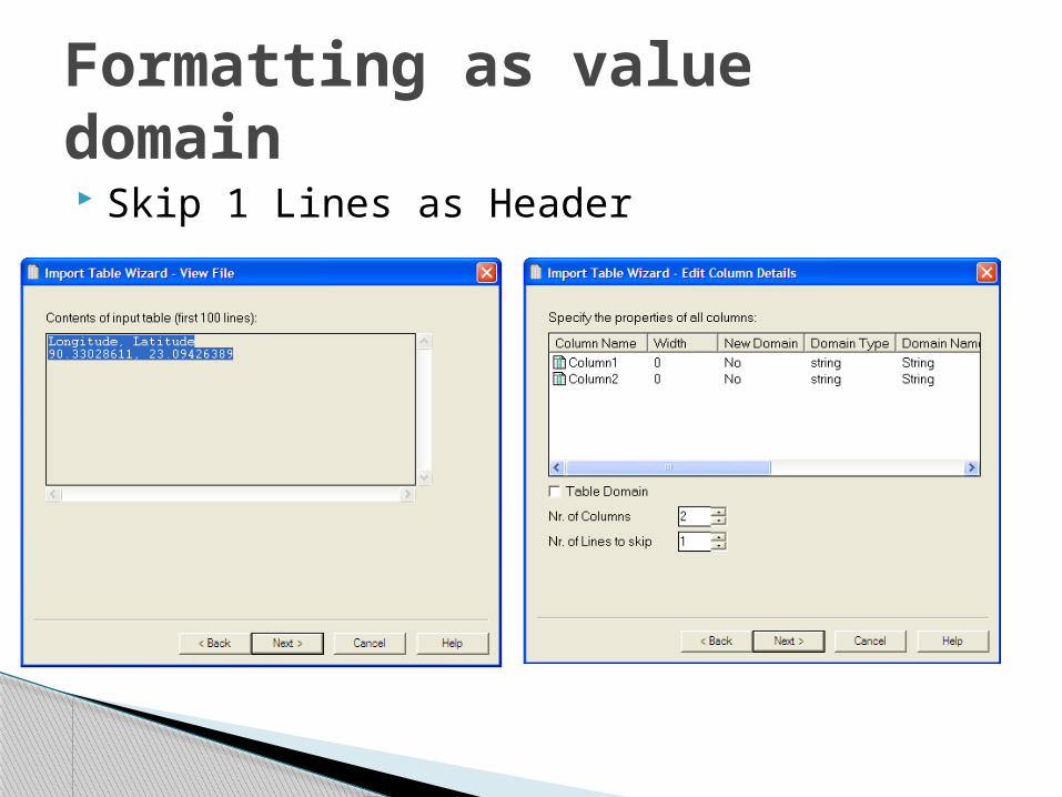
Skip 1 Lines as Header
Formatting as value domain
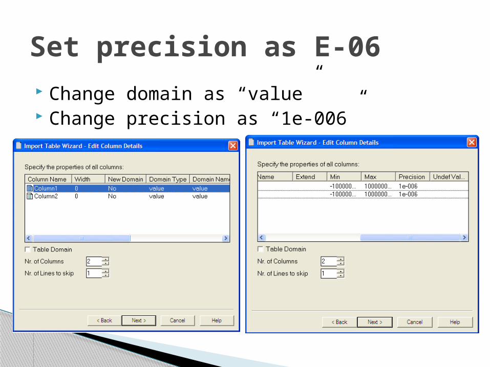
Change domain as “value” Change precision as “1e-006”
Set precision as E-06
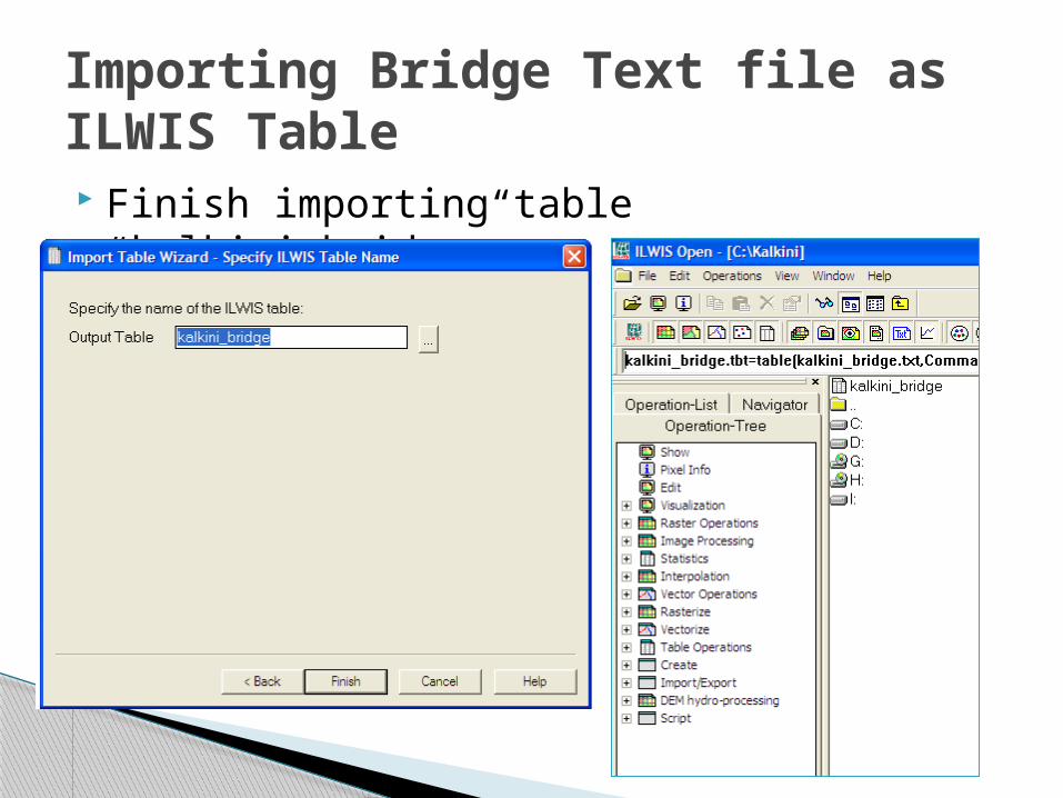
Finish importing table “kalkini_bridge”
Importing Bridge Text file as ILWIS Table
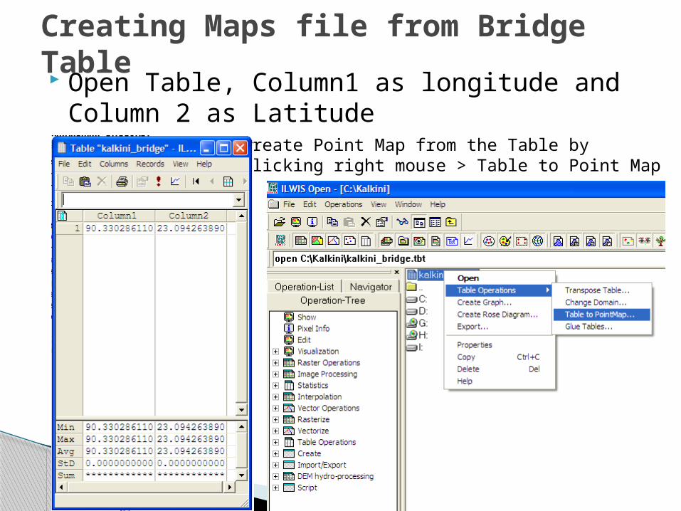
Open Table, Column1 as longitude and Column 2 as Latitude
Creating Maps file from Bridge Table
Create Point Map from the Table by Clicking right mouse > Table to Point Map
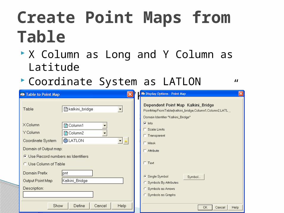
X Column as Long and Y Column as Latitude Coordinate System as LATLON Output PointMap “Kalkini_Bridge” > Show
Create Point Maps from Table
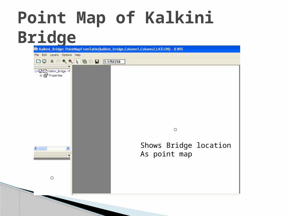
Point Map of Kalkini Bridge
Shows Bridge locationAs point map
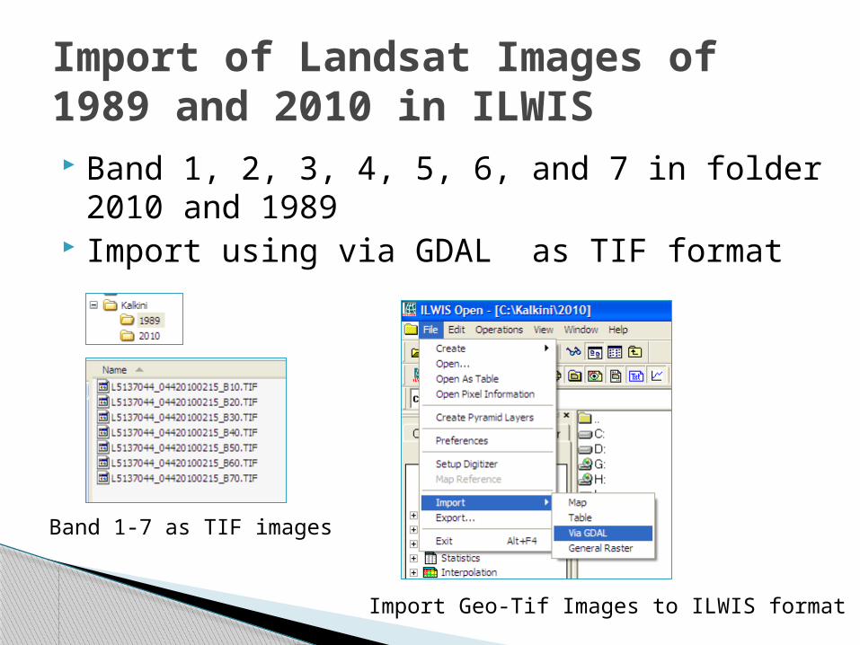
Band 1, 2, 3, 4, 5, 6, and 7 in folder 2010 and 1989
Import using via GDAL as TIF format
Import of Landsat Images of 1989 and 2010 in ILWIS
Band 1-7 as TIF images
Import Geo-Tif Images to ILWIS format
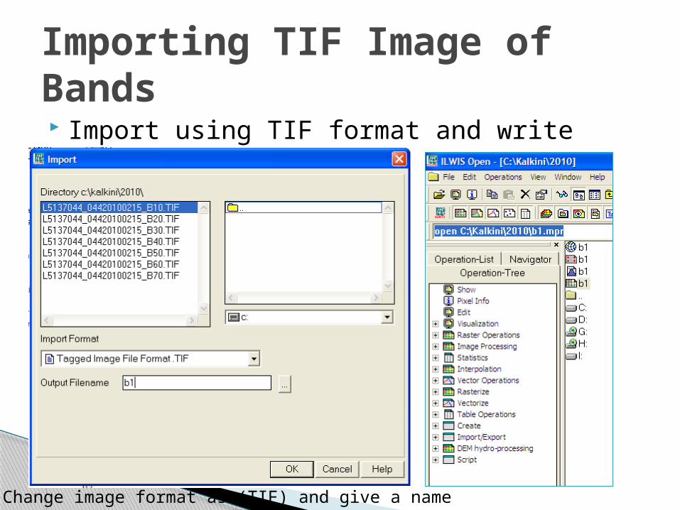
Import using TIF format and write file name
Importing TIF Image of Bands
Change image format as (TIF) and give a name
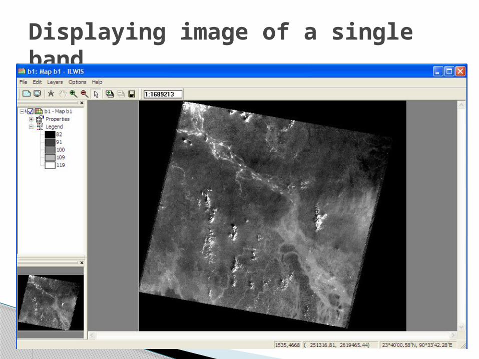
Displaying image of a single band
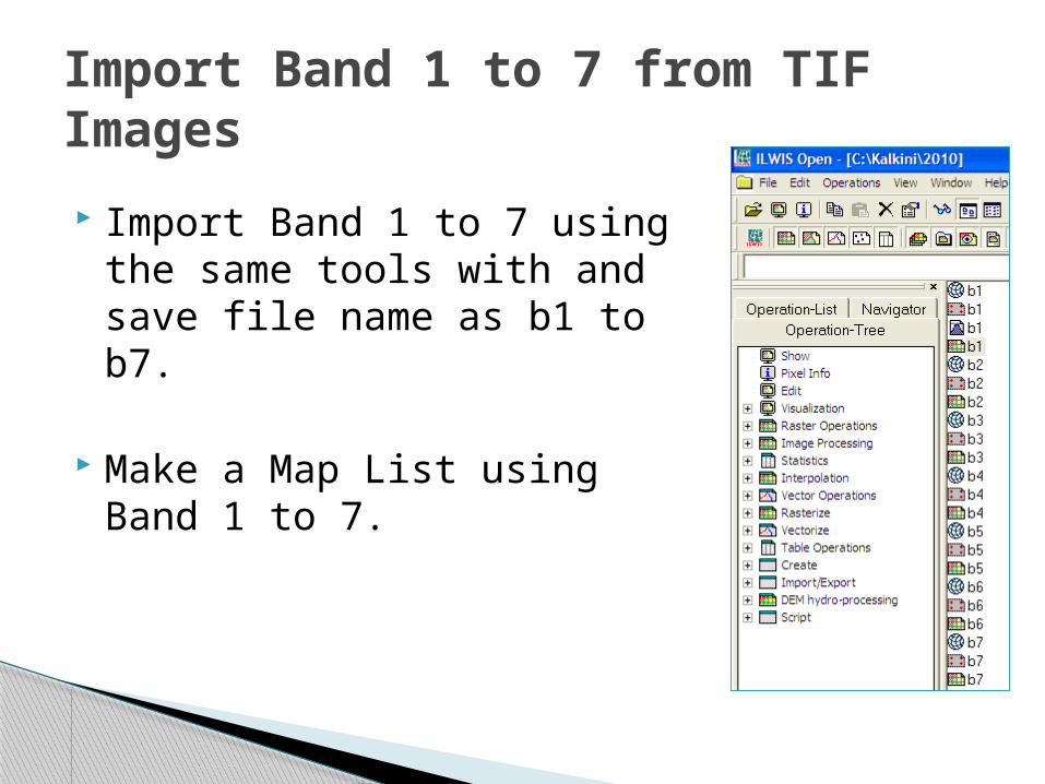
Import Band 1 to 7 using the same tools with and save file name as b1 to b7.
Make a Map List using Band 1 to 7.
Import Band 1 to 7 from TIF Images
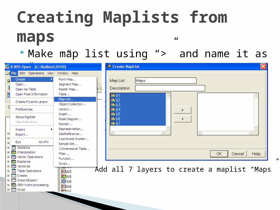
Make map list using “>” and name it as “maps”
Creating Maplists from maps
Add all 7 layers to create a maplist “Maps”

Select Bands (7-4-2) for false color composite maps
Use display tool
Select band 7-4-2 as RGB
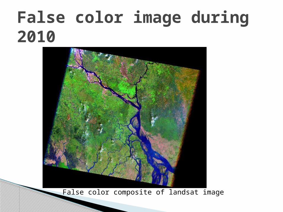
False color image during 2010
False color composite of landsat image
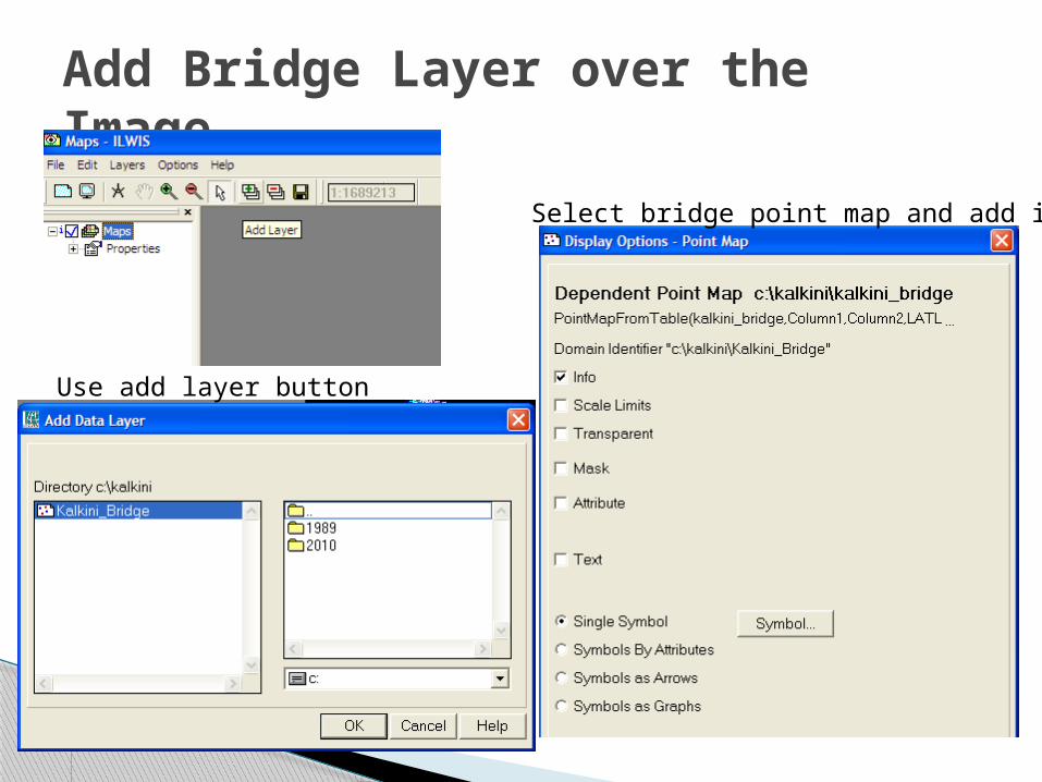
Add Bridge Layer over the Image
Use add layer button
Select bridge point map and add it

Insert Bridge location on false color composite maps
Change color to red
Location of the bridge in red color

Zoom over the Bridge Site
Use zoom tool
Zoom the map over bridge site

Creating Segment Maps of Bank
Create new segment For bank lines
Write segment names
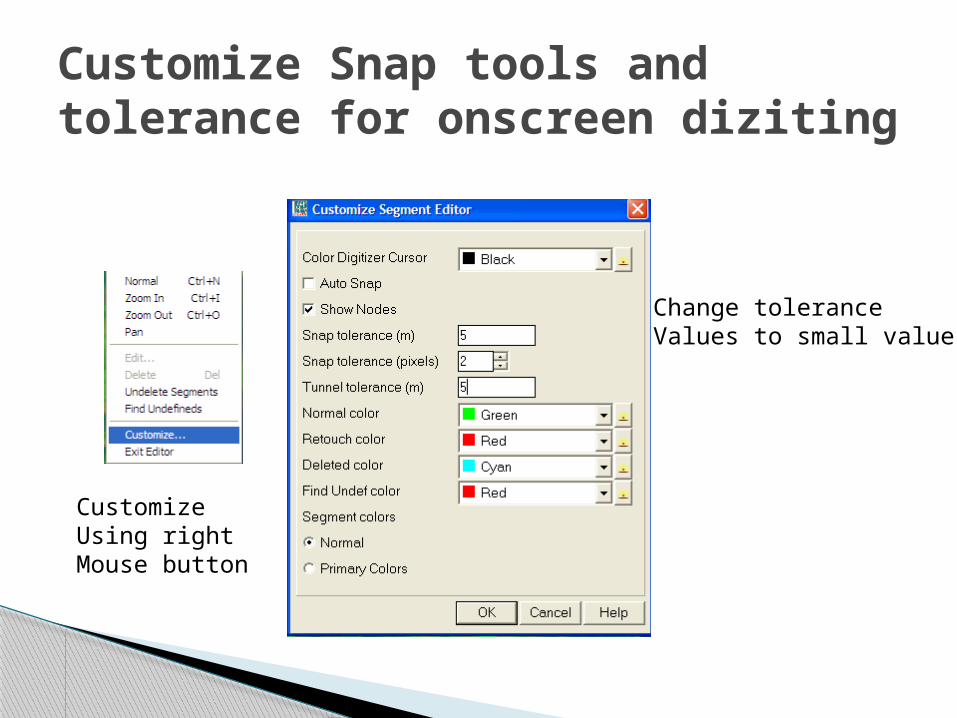
Customize Snap tools and tolerance for onscreen diziting
Change tolerance Values to small value
Customize Using right Mouse button
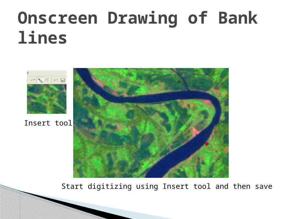
Onscreen Drawing of Bank lines
Start digitizing using Insert tool and then save
Insert tool
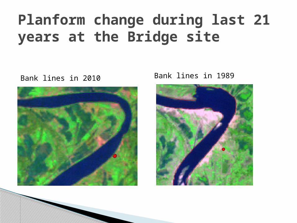
Planform change during last 21 years at the Bridge site
Bank lines in 2010 Bank lines in 1989

Change of Planforms using Images and Field verification
Field visit to the bridge site
Changes over 21 years
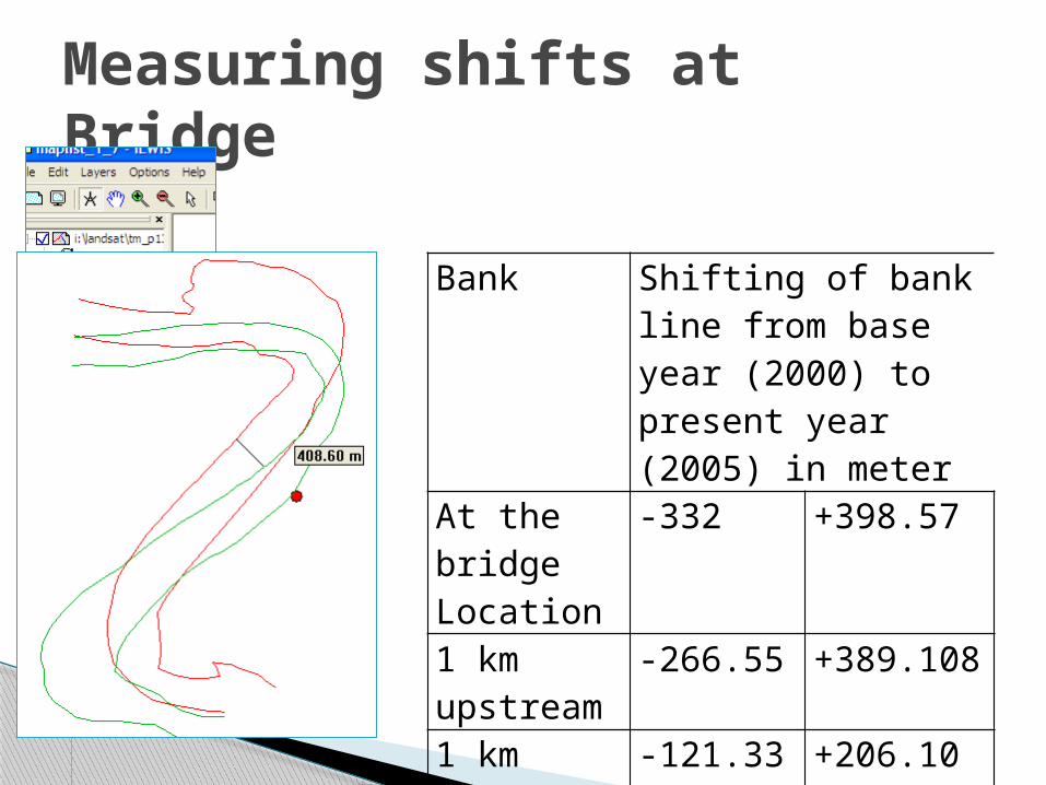
Bank Shifting of bank line from base year (2000) to present year (2005) in meter
At the bridge Location
-332 +398.57
1 km upstream
-266.55 +389.108
1 km down stream
-121.33 +206.10
Measuring shifts at Bridge
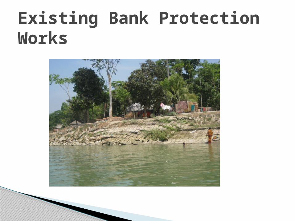
Existing Bank Protection Works

Thank you


