Embed Size (px)
Citation preview
THESIS
to be presented at
Universidad de La República, UdelaR
in order to obtain the title of
MAGISTER EN INGENIERÍA MATEMÁTICA
for
Eng. Javier PEREIRA LUCAS
Research Institute : LPE - IMERLUniversity Components :
UNIVERSIDAD DE LA REPÚBLICA
FACULTAD DE INGENIERÍA
Thesis title :
Routing cost optimization in Multi Overlay Robust Networks
to be presented on May 2013 to the Comitee of Examiners
Dr. Pablo BELZARENA Academic DirectorDr. Alvaro MARTIN Thesis DirectorDr. Franco ROBLEDO Thesis DirectorDr. Alejandra BEGHELLI PresidentDr. Gerardo RUBINODr. Martín VARELA RICO


Acknowledgements
This work is dedicated not only to those who helped me to deal with all the challenges I
faced in order to complete my thesis but also to those who gave me emotional support through-
out this time.
I would specially like to thank to my Thesis Directors, Dr. Franco Robledo and Dr. Alvaro
Martín, for the original idea of the thesis and for all the support I had to solve this problem.
I would also like to thank ANTEL, Uruguay’s biggest telecommunications service provider,
not only for supporting this work and the local research team with valuable information, but
also for helping in the development of many research groups in different research areas all over
the country.
Last but not least I would like to thank to the ones who are always present when I need
support, my family and friends.

Contents
Index 1
I INTRODUCTION 7
1 Introduction 9
1.1 Introduction . . . . . . . . . . . . . . . . . . . . . . . . . . . . . . . . . . . . 9
1.2 Problem Overview and Related work . . . . . . . . . . . . . . . . . . . . . . . 13
1.3 Thesis Organization . . . . . . . . . . . . . . . . . . . . . . . . . . . . . . . . 15
II PROBLEM DESCRIPTION AND FORMAL MODEL 17
2 Model Entities 19
2.1 Introduction . . . . . . . . . . . . . . . . . . . . . . . . . . . . . . . . . . . . 19
2.2 The Data Network . . . . . . . . . . . . . . . . . . . . . . . . . . . . . . . . 19
2.2.1 Data Traffic . . . . . . . . . . . . . . . . . . . . . . . . . . . . . . . . 20
2.3 The Transport Network . . . . . . . . . . . . . . . . . . . . . . . . . . . . . . 21
2.3.1 Transport Links . . . . . . . . . . . . . . . . . . . . . . . . . . . . . . 22
2.3.2 Transport Network Traffic . . . . . . . . . . . . . . . . . . . . . . . . 22
2.3.3 Transmission Costs . . . . . . . . . . . . . . . . . . . . . . . . . . . . 23
2.3.4 Installation Cost . . . . . . . . . . . . . . . . . . . . . . . . . . . . . 24
2.3.5 Installation Budget . . . . . . . . . . . . . . . . . . . . . . . . . . . . 24
2.4 Traffic Routing . . . . . . . . . . . . . . . . . . . . . . . . . . . . . . . . . . 25
2.4.1 Routing in the Data Network . . . . . . . . . . . . . . . . . . . . . . 25
2.4.2 Routing in the Transport Network . . . . . . . . . . . . . . . . . . . . 27
3 Formal Definition of the Problem 29
3.1 Structure of the Problem . . . . . . . . . . . . . . . . . . . . . . . . . . . . . 29
3.2 Formal Definition of the Problem . . . . . . . . . . . . . . . . . . . . . . . . . 30
1
2 Contents
III ALGORITHM AND RELEVANT PROPERTIES 33
4 An Algorithm for the MOBCRN 35
4.1 Design Alternatives . . . . . . . . . . . . . . . . . . . . . . . . . . . . . . . . 354.2 Algorithm Description . . . . . . . . . . . . . . . . . . . . . . . . . . . . . . 35
4.2.1 High Level Description . . . . . . . . . . . . . . . . . . . . . . . . . . 354.2.2 Low Level Description . . . . . . . . . . . . . . . . . . . . . . . . . . 37
4.2.2.1 Step 1: Nominal Routing on the Transport Network . . . . . 374.2.2.2 Step 2: Find Connected Subgraph . . . . . . . . . . . . . . . 414.2.2.3 Step 3: Build 2-Connected Graph . . . . . . . . . . . . . . . 444.2.2.4 Step 4: Simple Failure Routing . . . . . . . . . . . . . . . . 464.2.2.5 Step 5: Data Network Routing . . . . . . . . . . . . . . . . 504.2.2.6 Shortest Path Algorithm . . . . . . . . . . . . . . . . . . . . 55
4.2.3 Unfeasible Scenarios . . . . . . . . . . . . . . . . . . . . . . . . . . . 60
IV RESULTS 61
5 Test Cases Description 63
5.1 First Set of Test Cases . . . . . . . . . . . . . . . . . . . . . . . . . . . . . . . 635.1.1 Problem Data . . . . . . . . . . . . . . . . . . . . . . . . . . . . . . . 63
5.2 Performance Test Cases . . . . . . . . . . . . . . . . . . . . . . . . . . . . . . 67
6 Results of the Test Cases 71
6.1 Results of the First Set of Test Cases . . . . . . . . . . . . . . . . . . . . . . . 716.2 Results of the Second Set of Test Cases . . . . . . . . . . . . . . . . . . . . . 76
6.2.1 Test case number one . . . . . . . . . . . . . . . . . . . . . . . . . . . 796.2.2 Test case number two . . . . . . . . . . . . . . . . . . . . . . . . . . . 816.2.3 Test case number three . . . . . . . . . . . . . . . . . . . . . . . . . . 836.2.4 Test case number four . . . . . . . . . . . . . . . . . . . . . . . . . . 856.2.5 Conclusions . . . . . . . . . . . . . . . . . . . . . . . . . . . . . . . . 87
7 Conclusions 89
8 Open Problems and Future Work 91
Bibliography 96
List of Figures 97
Summary
In the present work we solve the problem of data flow routing in Multi-Overlay RobustNetworks (MORN) while aiming to minimize its routing cost. This kind of networks are typi-cally IP/MPLS Data Network deployed over an SDH/DWDM transport infrastructure.
Through the IP/MPLS Multi-Layer Data Network different kinds of services having a widevariety of quality of service requirements are delivered. Those services are being transported byan SDH/DWDM Transport Network which has different transport capacities. In this network,routing cost depends not only on the assigned transport capacity but also in the technology thatit uses.
Our problem seeks not only to route data flows through Data and Transport Networks butalso to optimize routing costs and the reliability of the network. The inputs of our problemare the topology of the Data and Transport networks as well as the budget that the networkoperator has in order to improve its network routing costs and reliability. We will assume thatthe operator can only use that budget for installing new links between existing transport nodes.The output of the problem is the data flow routing in the Data and Transport Networks andits associated cost. Routing in the Transport Network is calculated not only in the nominalscenario - when all the Transport Network links are up and running - but also in each singletransport link failure case.
3

4 Contents
Resumen
En el presente trabajo se resuelve el problema de rutear flujos de datos en una Red Multi-Capa Robusta (MORN por sus siglas en inglés), mientras que se trata de minimizar el costoasociado a su ruteo. Este tipo de redes son generalmente redes de datos IP/MPLS desplegadassobre una infraestructura de transporte SDH/DWDM.
Sobre la red de datos IP/MPLS se cursan distintos servicios con diferentes requerimientosde calidad de servicio (QoS). Los servicios de la Red de Datos son transportados por la redSDH/DWDM la cual tiene distintas capacidades de transporte. En éste tipo de redes el costoasociado al transporte depende no solo de la capacidad asignada para el transporte sino quetambién depende de la tecncología utilizada para transportar dicha capacidad.
En el problema no sólo se busca enrutar flujos de datos a través de las Redes de Datos yTransporte sino que también se busca optimizar los costos de ruteo y la confiabilidad de la red.Como punto de partida, el problema toma como información la topología de las Redes de Datosy Transporte así como cierto presupuesto que el operador de la red posee para poder mejorarlos costos de ruteo y la confiabilidad de su red. Asumiremos que dicho presupuesto solo puedeser utilizado para instalar nuevos enlaces entre los nodos existentes en la Red de Transporte.La salida del problema es el ruteo de los flujos de datos tanto en la Red de Datos como en lade Transporte, así como el costo asociado a dicho ruteo. El ruteo en la Red de Transporte secalcula no solo en el escenario nominal - cuando todos los enlaces de la Red de Transporteestán funcionales - sino que también en cada escenario de falla simple en sus enlaces.
5

6 Contents

Part I
INTRODUCTION
7

Chapter 1
Introduction
1.1 Introduction
Telecommunication networks play an extremely important role in our communities, allow-ing to share information in a wide range of activities. These activities span from entretainment(online gaming, social networking, etc) to all kind of critical activities such as science, educa-tion or health.
In last years most telecommunication companies started deploying optical fiber networks.Throughout this work, this optical network will be refered to as the physical network. To guar-antee service availability, these networks were designed in a way that several independent pathsare available between each pair of nodes. As optimizing budget allocation is a key requirementfor operators, several algorithms were developed to address this point. Many research groupsin works as [23, 25, 30] have been working for many time in this area.
The exponential growth of Internet traffic volume led to the deployment of Dense Wave-length Division Multiplexing (DWDM) technology [5]. This technology allows multiplexingseveral connections over one single optical fiber using different wavelengths, and rapidly be-came very popular with telecommunications companies because it allowed them to expandthe capacity of their networks without laying more optical fiber. A DWDM link is a logicalconnection between two nodes that have an optical fiber connection. A DWDM path is a setof links that connects, from a logical point of view, two remote nodes. Nowadays, DWDM isthe most popular network technology in high-capacity optical backbone networks. Optical re-peaters must be placed at regular intervals for compensating the loss in optical power while thesignal travels along the fiber. Therefore, the cost of a DWDM path is proportional to its lengthover the physical network.
DWDM supports a set of standard high-capacity interfaces (e.g. 1, 2.5, 10 or 40 Gbps). Thecost of a connection also depends on the capacity but not proportionally. Due to economies ofscale, the higher the bit-rate the lower is the ratio cost per capacity. DWDM nodes and pathsform a so-called transport network. This network runs on top of the physical one.
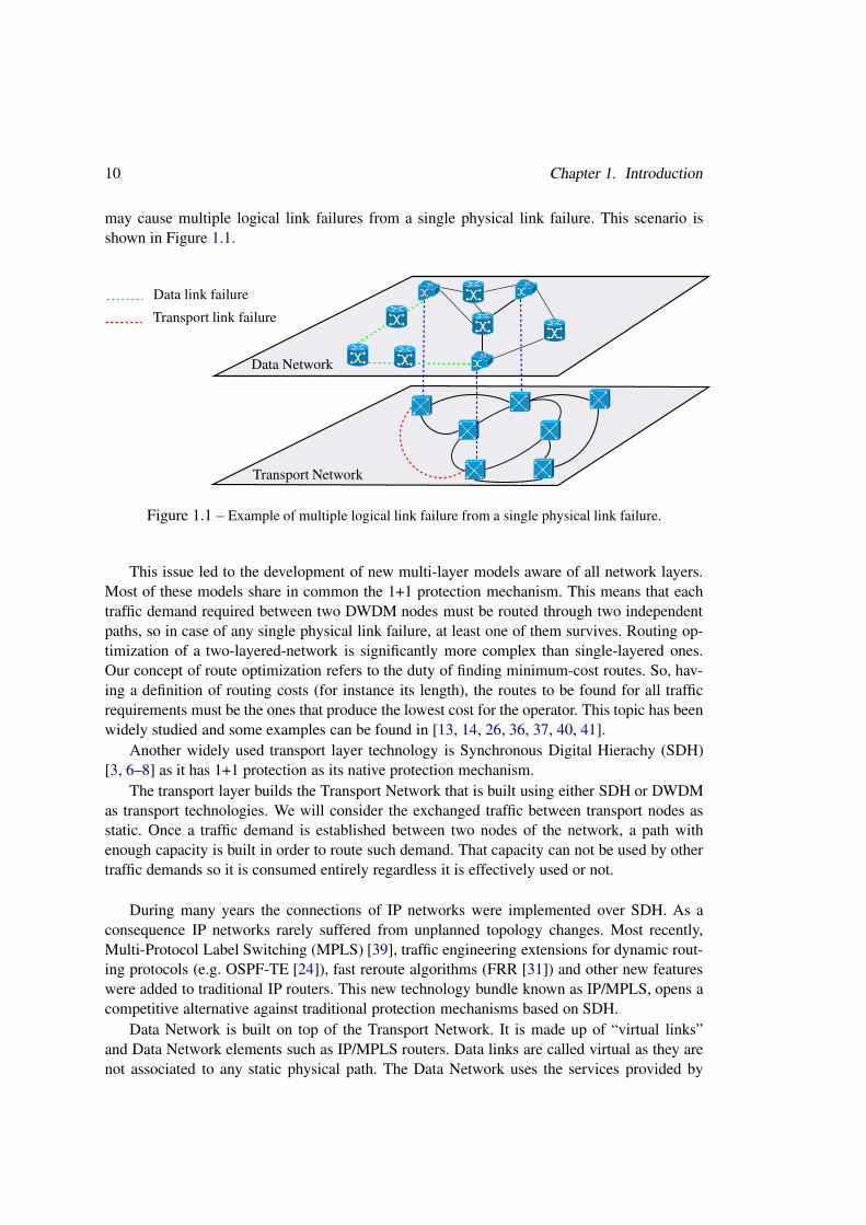
As traffic grows, the number of DWDM links per physical connection must increase. This
9
10 Chapter 1. Introduction
may cause multiple logical link failures from a single physical link failure. This scenario isshown in Figure 1.1.
Data Network
Transport Network
Data link failure
Transport link failure
Figure 1.1 – Example of multiple logical link failure from a single physical link failure.
This issue led to the development of new multi-layer models aware of all network layers.Most of these models share in common the 1+1 protection mechanism. This means that eachtraffic demand required between two DWDM nodes must be routed through two independentpaths, so in case of any single physical link failure, at least one of them survives. Routing op-timization of a two-layered-network is significantly more complex than single-layered ones.Our concept of route optimization refers to the duty of finding minimum-cost routes. So, hav-ing a definition of routing costs (for instance its length), the routes to be found for all trafficrequirements must be the ones that produce the lowest cost for the operator. This topic has beenwidely studied and some examples can be found in [13, 14, 26, 36, 37, 40, 41].
Another widely used transport layer technology is Synchronous Digital Hierachy (SDH)[3, 6–8] as it has 1+1 protection as its native protection mechanism.
The transport layer builds the Transport Network that is built using either SDH or DWDMas transport technologies. We will consider the exchanged traffic between transport nodes asstatic. Once a traffic demand is established between two nodes of the network, a path withenough capacity is built in order to route such demand. That capacity can not be used by othertraffic demands so it is consumed entirely regardless it is effectively used or not.
During many years the connections of IP networks were implemented over SDH. As aconsequence IP networks rarely suffered from unplanned topology changes. Most recently,Multi-Protocol Label Switching (MPLS) [39], traffic engineering extensions for dynamic rout-ing protocols (e.g. OSPF-TE [24]), fast reroute algorithms (FRR [31]) and other new featureswere added to traditional IP routers. This new technology bundle known as IP/MPLS, opens acompetitive alternative against traditional protection mechanisms based on SDH.
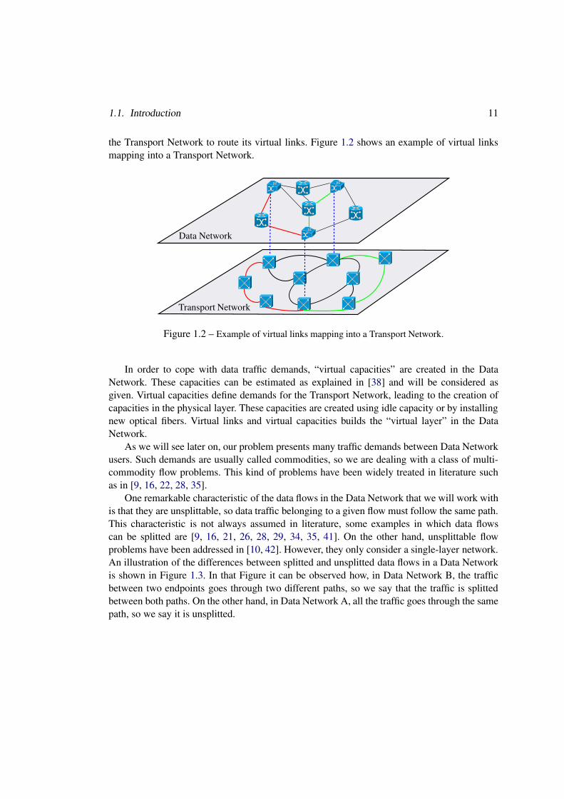
Data Network is built on top of the Transport Network. It is made up of “virtual links”and Data Network elements such as IP/MPLS routers. Data links are called virtual as they arenot associated to any static physical path. The Data Network uses the services provided by
1.1. Introduction 11
the Transport Network to route its virtual links. Figure 1.2 shows an example of virtual linksmapping into a Transport Network.
Data Network
Transport Network
Figure 1.2 – Example of virtual links mapping into a Transport Network.
In order to cope with data traffic demands, “virtual capacities” are created in the DataNetwork. These capacities can be estimated as explained in [38] and will be considered asgiven. Virtual capacities define demands for the Transport Network, leading to the creation ofcapacities in the physical layer. These capacities are created using idle capacity or by installingnew optical fibers. Virtual links and virtual capacities builds the “virtual layer” in the DataNetwork.
As we will see later on, our problem presents many traffic demands between Data Networkusers. Such demands are usually called commodities, so we are dealing with a class of multi-commodity flow problems. This kind of problems have been widely treated in literature suchas in [9, 16, 22, 28, 35].
One remarkable characteristic of the data flows in the Data Network that we will work withis that they are unsplittable, so data traffic belonging to a given flow must follow the same path.This characteristic is not always assumed in literature, some examples in which data flowscan be splitted are [9, 16, 21, 26, 28, 29, 34, 35, 41]. On the other hand, unsplittable flowproblems have been addressed in [10, 42]. However, they only consider a single-layer network.An illustration of the differences between splitted and unsplitted data flows in a Data Networkis shown in Figure 1.3. In that Figure it can be observed how, in Data Network B, the trafficbetween two endpoints goes through two different paths, so we say that the traffic is splittedbetween both paths. On the other hand, in Data Network A, all the traffic goes through the samepath, so we say it is unsplitted.

12 Chapter 1. Introduction
Data Network A Data Network B
Figure 1.3 – Illustration of a Data Network implementing unsplitted (A) and splitted (B) data flows.
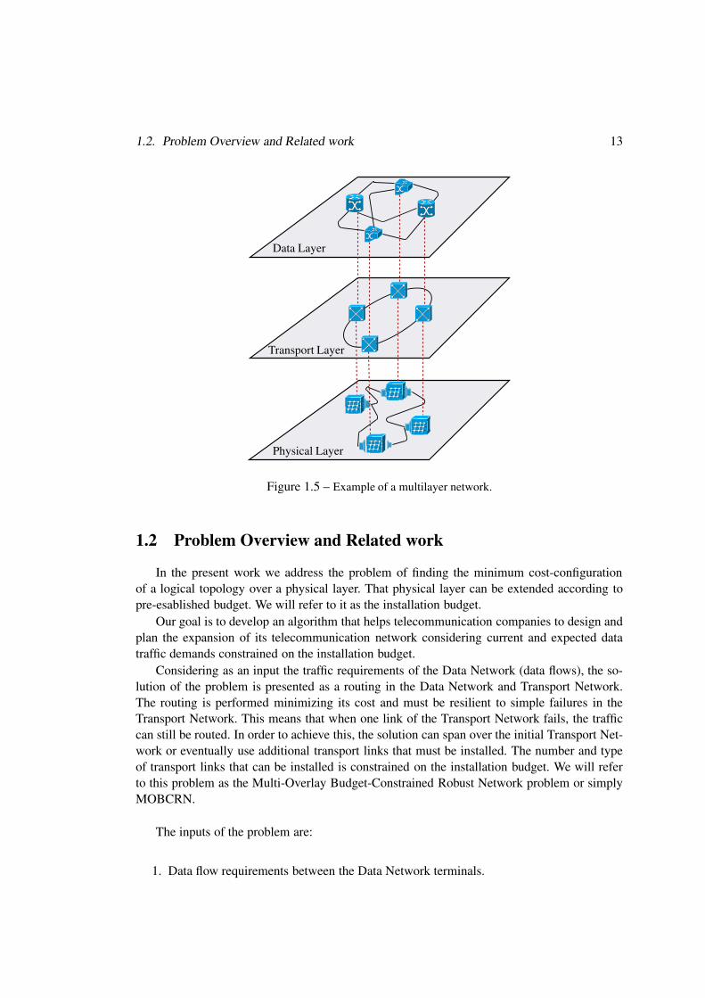
IP/MPLS networks are usually represented in a stack diagram like the Open System Inter-connection (OSI) basic reference model that is defined in the ITU-T X.200 recommendation[4]. Figure 1.4 shows the interaction of different layers in a stack diagram. Figure 1.5 showsa network diagram of a multilayer structure. Layer 1 represents the Physical network, Layer 2represents the Transport Network and Layer 3 represents the Data Network.
Figure 1.4 – Examples of different technologies interacting in a stack structure.
1.2. Problem Overview and Related work 13
Data Layer
Transport Layer
Physical Layer
Figure 1.5 – Example of a multilayer network.
1.2 Problem Overview and Related work
In the present work we address the problem of finding the minimum cost-configurationof a logical topology over a physical layer. That physical layer can be extended according topre-esablished budget. We will refer to it as the installation budget.
Our goal is to develop an algorithm that helps telecommunication companies to design andplan the expansion of its telecommunication network considering current and expected datatraffic demands constrained on the installation budget.
Considering as an input the traffic requirements of the Data Network (data flows), the so-lution of the problem is presented as a routing in the Data Network and Transport Network.The routing is performed minimizing its cost and must be resilient to simple failures in theTransport Network. This means that when one link of the Transport Network fails, the trafficcan still be routed. In order to achieve this, the solution can span over the initial Transport Net-work or eventually use additional transport links that must be installed. The number and typeof transport links that can be installed is constrained on the installation budget. We will referto this problem as the Multi-Overlay Budget-Constrained Robust Network problem or simplyMOBCRN.
The inputs of the problem are:
1. Data flow requirements between the Data Network terminals.
14 Chapter 1. Introduction
2. Data Network and Transport Network topologies.
3. The budget to install new links.
4. The cost of installing each potential new link in the Transport Network.
The Data Network spans over a network that can be modeled using a complete graph. Thismeans that every data node can establish a link with any other data node in the Data Network.This can be justified by the fact that Data Network nodes are connected through virtual linksthat are established dinamically once a data flow needs to be routed.
As the Transport Network usually has a topology structured in rings, we can model it asthe composition of one or more cycles.
As we mentioned earlier, to solve our problem we must route data flows in the Data Net-work and Transport Network targeting to optimize the routing costs. In case it is necessary andpossible, this is achieved by expanding the Transport Network installing new links.
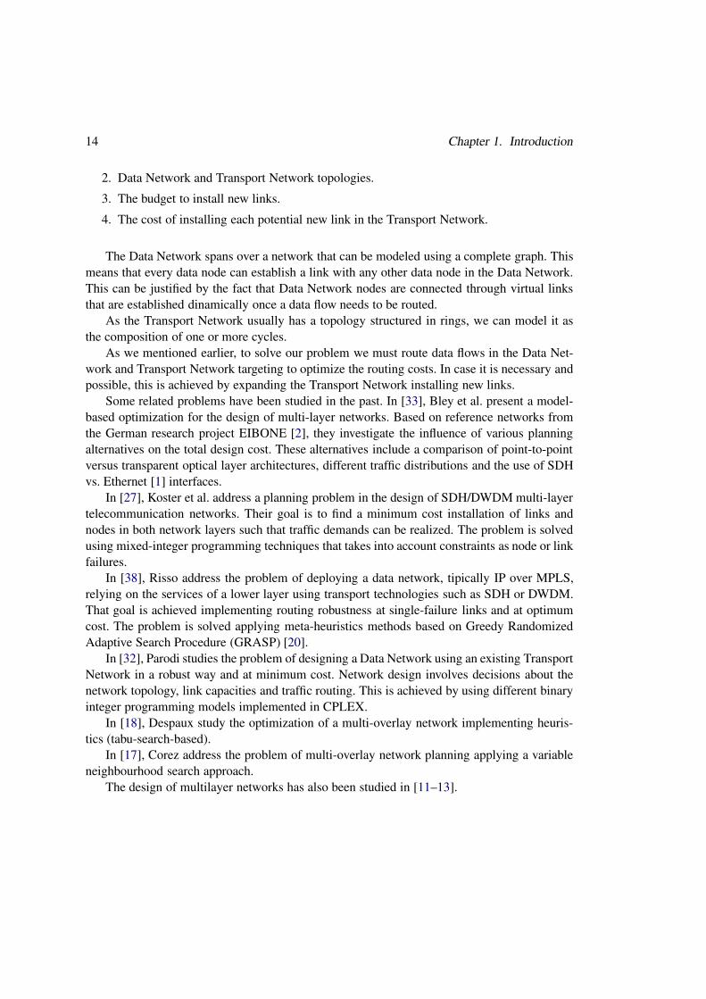
Some related problems have been studied in the past. In [33], Bley et al. present a model-based optimization for the design of multi-layer networks. Based on reference networks fromthe German research project EIBONE [2], they investigate the influence of various planningalternatives on the total design cost. These alternatives include a comparison of point-to-pointversus transparent optical layer architectures, different traffic distributions and the use of SDHvs. Ethernet [1] interfaces.
In [27], Koster et al. address a planning problem in the design of SDH/DWDM multi-layertelecommunication networks. Their goal is to find a minimum cost installation of links andnodes in both network layers such that traffic demands can be realized. The problem is solvedusing mixed-integer programming techniques that takes into account constraints as node or linkfailures.
In [38], Risso address the problem of deploying a data network, tipically IP over MPLS,relying on the services of a lower layer using transport technologies such as SDH or DWDM.That goal is achieved implementing routing robustness at single-failure links and at optimumcost. The problem is solved applying meta-heuristics methods based on Greedy RandomizedAdaptive Search Procedure (GRASP) [20].
In [32], Parodi studies the problem of designing a Data Network using an existing TransportNetwork in a robust way and at minimum cost. Network design involves decisions about thenetwork topology, link capacities and traffic routing. This is achieved by using different binaryinteger programming models implemented in CPLEX.
In [18], Despaux study the optimization of a multi-overlay network implementing heuris-tics (tabu-search-based).
In [17], Corez address the problem of multi-overlay network planning applying a variableneighbourhood search approach.
The design of multilayer networks has also been studied in [11–13].

1.3. Thesis Organization 15
1.3 Thesis Organization
The rest of this thesis is organized as follows:
Chapter 2: Model Entities, introduces the network elements and mathematical conceptsthat compose the MOBCRN problem.
Chapter 3: Formal Definition of the Problem, explains the abstract model and the structureof the problem.
Chapter 4: An Algorithm for the MOBCRN, explains step-by-step how the algorithmworks.
Chapter 5: Test Cases Description, describes all the test cases implemented in order tovalidate and explore the functionalities of the algorithm designed.
Chapter 6: Results of the Test Cases, shows the results obtained when running the set oftest cases explained in the aforementioned chapter.
Chapter 7: Conclusions, summarizes the project and presents the conclusions.
Chapter 8: Open Problems and Future Work, presents some open problems that can bestudied taking the present work as base.

16 Chapter 1. Introduction
Part II
PROBLEM DESCRIPTION AND
FORMAL MODEL
17

Chapter 2
Model Entities
2.1 Introduction
This chapter introduce the network elements that are part of the MOBCRN problem. Wedefine the Data and Transport Network with their different elements and characteristics andhow we model the costs. We also explain the relation between Data and Transport Networksand the routing within each network. Finally, we define the problem formally.
2.2 The Data Network
Definition 2.2.1 A Data Network graph is a simple undirected graph, GD = (VD, ED), where
VD represents the set of data nodes and ED represents the set of edges.
GD = (VD,ED) topology: The Data Network graph can be either a simple graph or amulti-graph. For convinience we will assume that the Data Network graph is a simple graphwhose edges can eventually represent as much parallel edges as necessary.
We will also consider that the graph is undirected. This means that given any edge ed ∈ ED
that connects two data nodes va, vb ∈ VD, the communication between both nodes is bi-directional and full duplex. This is the same as having two uni-directional edges between bothnodes compacted into just one node.
Finally, we also must consider the different alternatives for the connection between datanodes. We will consider that every node vd ∈ VD can be directly connected to each other.
19
20 Chapter 2. Model Entities
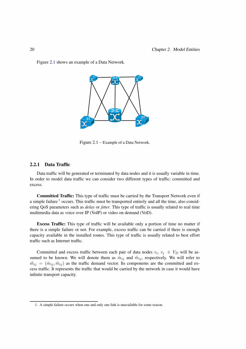
Figure 2.1 shows an example of a Data Network.
Figure 2.1 – Example of a Data Network.
2.2.1 Data Traffic
Data traffic will be generated or terminated by data nodes and it is usually variable in time.In order to model data traffic we can consider two different types of traffic: committed andexcess.
Committed Traffic: This type of traffic must be carried by the Transport Network even ifa simple failure 1 occurs. This traffic must be transported entirely and all the time, also consid-ering QoS parameters such as delay or jitter. This type of traffic is usually related to real timemultimedia data as voice over IP (VoIP) or video on demand (VoD).
Excess Traffic: This type of traffic will be available only a portion of time no matter ifthere is a simple failure or not. For example, excess traffic can be carried if there is enoughcapacity available in the installed routes. This type of traffic is usually related to best efforttraffic such as Internet traffic.
Committed and excess traffic between each pair of data nodes vi, vj ∈ VD will be as-sumed to be known. We will denote them as mij and mij , respectively. We will refer to~mij = (mij, mij) as the traffic demand vector. Its components are the committed and ex-cess traffic. It represents the traffic that would be carried by the network in case it would haveinfinite transport capacity.
1. A simple failure occurs when one and only one link is unavailable for some reason.
2.3. The Transport Network 21
Definition 2.2.2 Function f , f : R2 → R, maps the traffic demand vector, ~mij = (mij , mij),in a single real value, mij which is the estimated traffic demand. More details about how this
function operates can be found in [38].
Definition 2.2.3 We will refer to M = [mij ]1≤i,j≤|VD| as the demand matrix of the problem. It
is a matrix whose elements mij = f(mij, mij) represent the demand between vi and vj .
2.3 The Transport Network
The Transport Network will be represented by a simple, non-directed, planar, 2-vertex-connected graph. We can assume that the graph is planar as the optical fiber canalizations are.In case links must be overlapped we can install a network station on the overlapping point.
Definition 2.3.1 A Transport Network graph is a graph, GT = (VT , ET ), where VT and ET
represents the set of nodes and links of a Transport Network, respectively.
GT = (VT,ET) topology: The Transport Network graph can be designed with or withoutlink protection. As per “link protection” we understand the possibility of route a flow by twoedge-disjoint paths in GT . This enables a transport node to switch between these paths if a linkfailure occurs in one of them. We will consider that the topology of the Transport Network issuch that for every two nodes vr, vs ∈ VT there are at least two edge-disjoint paths that con-nect them. The most typical configuration that represents this scenario is a multi-ring topology.This is the most common topology used in SDH networks as SDH network elements has thecapability of switching the traffic from one side of the ring to another in a few miliseconds(tipically less than 50 ms). We can say that the Transport Network is 2-vertex-connected as it isbuilt upon the transport “rings” concatenation which always have at least two nodes in common.
Definition 2.3.2 In same situations the telecommunication network will share a Data Network
and a Transport Network node in the same building. Function tns, tns : VD → VT , is such that
tns(vd) = vt when this situation happen. This function returns the transport node vt located
in the same Network Station as the data node vd.
22 Chapter 2. Model Entities
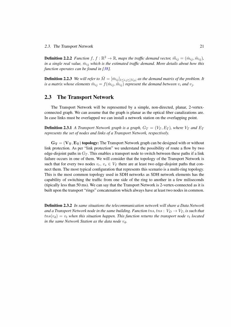
Figure 2.2 shows an example of a Transport Network.
Figure 2.2 – Example of a Transport Network.
2.3.1 Transport Links
Transport links does not have any capacity limit. This means that we must install as much“transport resources” as needed to cope with Data Network traffic demand. Transport resourcescan be optical fibers, processing or switching boards and even a whole new transport equip-ment.
Another consideration is that, according to our modeling, a failure in a transport link affectsall the connections that are being transported through that link. Although it is possible that notall the optical fibers corresponding to the same link fail at the same time, in general, opticalfiber failures are caused by external factors such as canalization damages that usually affectsall optical fibers corresponding to that canalization.
2.3.2 Transport Network Traffic
Transport Network traffic is completely static. Once a traffic demand is established betweentwo endpoints - a traffic flow - we need to find a path between these endpoints. That path musthave enough capacity to cope with the traffic demand and once it is established the requiredbandwidth is removed from the capacity of the links that compose that path. As we statedbefore, in order to achieve this we will install as many links as needed to match traffic demandneeds.
The same happens with routing. Once a route flow is established it remains static. Whensome link fails, all flows that are being carried through that link are out of service until that link
2.3. The Transport Network 23
becomes available again.
2.3.3 Transmission Costs
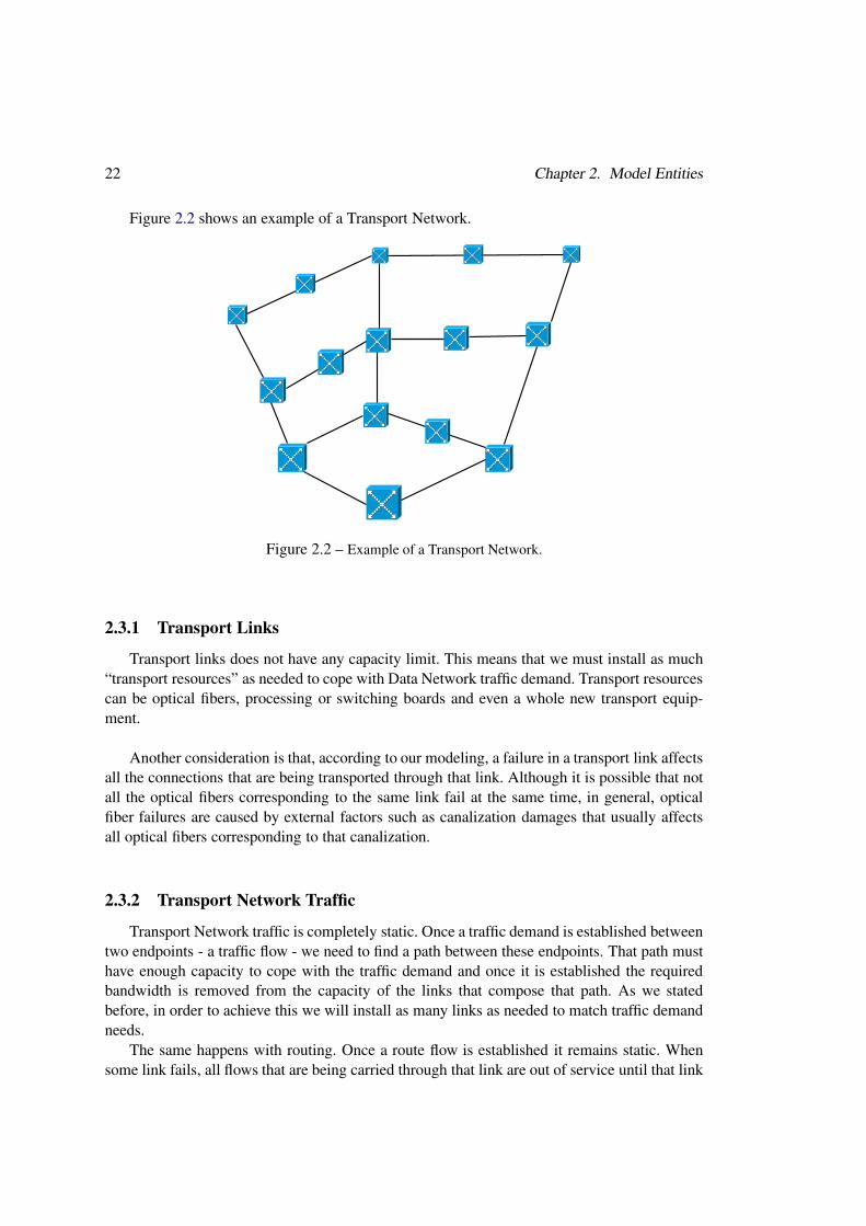
In Time Division Multiplex (TDM) technologies, such as SDH, the transmission cost of aflow is proportional to the product of the length of the route and the bandwidth of the flow.The traffic is transported in containers which have fixed bandwidths. In the case of opticaltechnologies, such as DWDM, the assigned resource to transport traffic is not a container but awavelength over which a wide variety of speeds can be modulated. In this case, costs are onlyproportional to the length of the route.
SDH and DWDM cost per kilometer are represented in Figure 2.3 in red and blue, respec-tively. The green line represents the minimum cost per kilometer for a given speed. This is themodel that we will assume for costs in the Transport Network.
Figure 2.3 – Cost per transport technology.

24 Chapter 2. Model Entities
Definition 2.3.3 We will consider B = {b0, b1, . . . , bB} as the set of capacities supported by
the connections of the Transport Network. By definition we will suppose that b0 = 0.
Definition 2.3.4 The cost function, T : B → R, maps each capacity of B to the corresponding
cost.
Definition 2.3.5 The distance function, r : ET → R, maps each edge et ∈ ET to its length
(say, in kilometers). We extend r to paths over GT by defining r(ρijT ) as the sum of r(et) over
all edges et of the path ρijT .
Definition 2.3.6 The cost in the Transport Network of a flow over a path ρijT with bandwidth
bij is cost(ρijT , bij) = r(ρijT )× T (bij).
2.3.4 Installation Cost
As part of the construction of a routing strategy we allow, under a budget constrain, theinstallation of new transport links.
Definition 2.3.7 Let ET be the set of potential edges to be added to the Transport Network.
We have ET = K|VT | \ET .
Definition 2.3.8 Let ET be the expanded set of edges. ET = ET ∪ {ei} where ei=0...|ET | are
the links that are added when expanding the Transport Network.
We will assume that installation cost of a new transport link depends linearly on its length.This is because most of installation costs can be associated to the cost of the optical fiber andthe canalization cost.
Definition 2.3.9 The installation cost matrix C = {cij}(i,j)∈ET, is a positive-real-cost matrix
associated to the arcs of ET = {K|VT | \ ET } that models the cost of installing a link between
two different sites of VT .
2.3.5 Installation Budget
We will consider that the operator has a budget that can be used to expand its TransportNetwork aiming to reduce and optimize its routing costs.
Definition 2.3.10 We will refer to I as the installation budget. It is the budget that the operator
can invest on its Transport Network.
2.4. Traffic Routing 25
2.4 Traffic Routing
2.4.1 Routing in the Data Network
The problem of routing in the Data Network is to find how to exchange traffic between anypair of nodes. That is, which are the links in the Data Network that we will use to route thetraffic. In an MPLS network these links builds a tunnel.
Notation 2.4.1 We denote by PD be the set of all possible paths in GD .
Definition 2.4.2 A routing scenario ρD is any subset of PD .
Definition 2.4.3 A routing scenario ρD is a set of paths over GD , each connecting a different
pair of data nodes, vi, vj , with (vi, vj) ∈ ED. We define for (vi, vj) ∈ ED, ρijD as the unique
path in ρD that connects vi with vj , if such a path exists. We write ρijD = ∅ otherwise.
Let’s the following example illustrate these definitions.
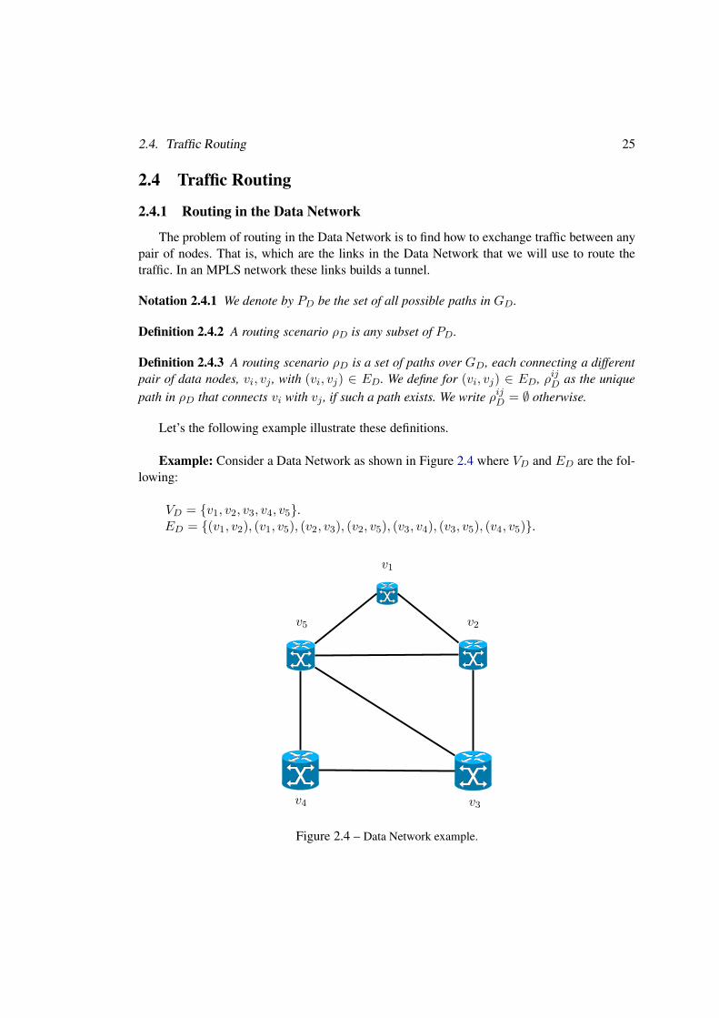
Example: Consider a Data Network as shown in Figure 2.4 where VD and ED are the fol-lowing:
VD = {v1, v2, v3, v4, v5}.ED = {(v1, v2), (v1, v5), (v2, v3), (v2, v5), (v3, v4), (v3, v5), (v4, v5)}.
v1
v2
v3v4
v5
Figure 2.4 – Data Network example.
26 Chapter 2. Model Entities
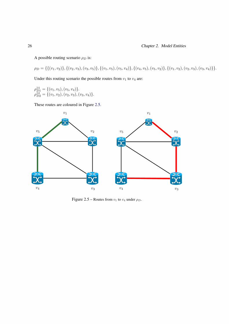
A possible routing scenario ρD is:
ρD = {{(v1, v2)}, {(v2, v3), (v3, v5)}, {(v1, v5), (v5, v4)}, {(v4, v5), (v5, v2)}, {(v1, v2), (v2, v3), (v3, v4)}}.
Under this routing scenario the possible routes from v1 to v4 are:
ρ14D1 = {(v1, v5), (v5, v4)}.ρ14D2 = {(v1, v2), (v2, v3), (v3, v4)}.
These routes are coloured in Figure 2.5.
v1 v1
v2 v2
v3 v3v4 v4
v5 v5
Figure 2.5 – Routes from v1 to v4 under ρD.
2.4. Traffic Routing 27
We next relate Transport and Data Network routing through the following definitions.
Definition 2.4.4 A routing scenario function, Φ : (ET ∪∅) → 2PD , assigns a routing scenario
for each edge et ∈ ET , as well as the empty set. For each et ∈ ET , Φ(et) represents a routing
scenario in case of failure of the link represented by et. We refer to Φ(∅) as the nominal routing
scenario; which represents a routing scenario in case all transport links are operative.
Notation 2.4.5 We denote by ρijDt∈ Φ(et) the routing in the Data Network between data nodes
vi and vj when the transport link represented by et is not operative.
2.4.2 Routing in the Transport Network
The problem of routing in the Transport Network is to set up the links that will provide thetransport service to the Data Network.
Notation 2.4.6 We denote by PT the set of all possible paths in GT .
Definition 2.4.7 A flow configuration ρT is a set of paths over GT , each connecting a different
pair of nodes, ti, tj , (ti, tj) ∈ ET . For a data edge ed = (vi, vj), we denote by ρijT the unique
path in ρT that connects tns(vi) with tns(vj), if it exists, and we denote ρijT = ∅ otherwise.
Definition 2.4.8 A flow configuration function, Ψ(vi, vj) = ρijT , assigns a flow configuration
to each edge in the Data Network.
The following example illustrates these concepts.
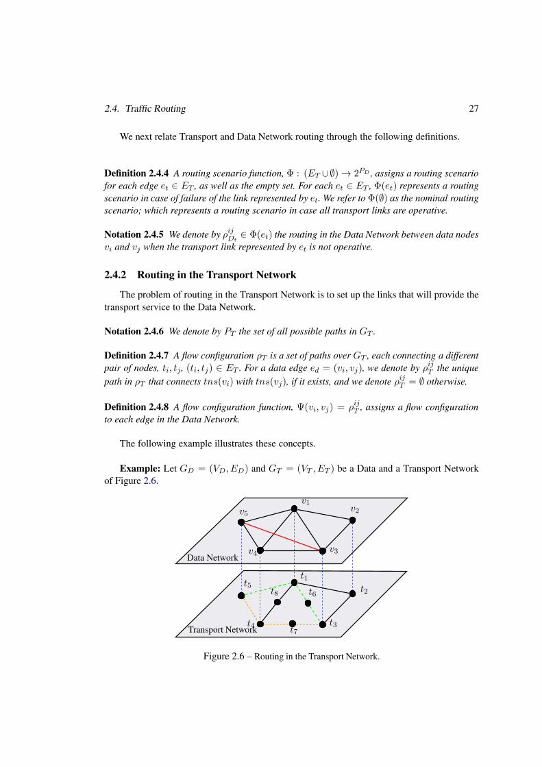
Example: Let GD = (VD, ED) and GT = (VT , ET ) be a Data and a Transport Networkof Figure 2.6.
Data Network
Transport Network
v1v2
v3v4
v5
t1t2
t3t4
t5t6
t7
t8
Figure 2.6 – Routing in the Transport Network.
28 Chapter 2. Model Entities
We have:
VD = {v1, v2, v3, v4, v5}.ED = {(v1, v2), (v2, v3), (v3, v4), (v3, v5), (v3, v1), (v4, v5), (v4, v1), (v5, v1)}.
VT = {t1, t2, t3, t4, t5, t6, t7, t8}.ET = {(t1, t2), (t2, t3), (t3, t7), (t3, t6), (t7, t4), (t4, t8), (t4, t5), (t5, t1), (t6, t1), (t8, t1)}.
tns(vi) = ti i = 1 . . . 5.
A possible flow configuration is:
ρT = {{(t1, t6), (t6, t3)}, {(t1, t2)}, {(t1, t8), (t8, t4)}, {(t5, t1), (t1, t6), (t6, t3)}, {(t1, t2), (t2, t3)},{(t5, t4), (t4, t7), (t7, t3)}}.
For example, under this flow configuration, ρ53T can be either {(t5, t1), (t1, t6), (t6, t3)} or{(t5, t4), (t4, t7), (t7, t3)}.
Chapter 3
Formal Definition of the Problem
3.1 Structure of the Problem
The structure of the problem is the following:
Inputs:
1. Data Network :
• GD = (VD,ED) : Data Network graph.• M : Traffic matrix.
2. Transport Network :
• GT = (VT,ET) : Transport Network graph.• B : Available capacities.• T : Technology cost function.• r : Distance function.• tns : Transport Network station function.• C : Installation costs matrix.• I : Installation budget.
Outputs:
1. GT = (VT, ET) : The expanded Transport Network.
2. B = {bij}(i,j)∈ED: Capacities assigned to the data links.
3. Φ = {ρijDt}i,j∈VD,t∈{∅∪ET} : Data routes for each failure scenario as well as the nominal
scenario.
4. Ψ = {ρijT}(i,j)∈ED,bij 6=0 : Transport routes for each data link in which a capacity is as-signed.
29
30 Chapter 3. Formal Definition of the Problem
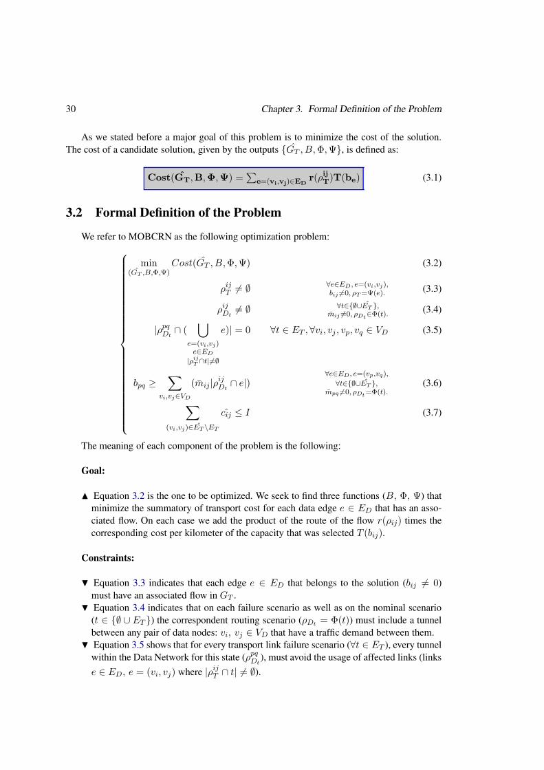
As we stated before a major goal of this problem is to minimize the cost of the solution.The cost of a candidate solution, given by the outputs {GT , B,Φ,Ψ}, is defined as:
Cost(GT,B,Φ,Ψ) =∑
e=(vi,vj)∈EDr(ρijT)T(be) (3.1)
3.2 Formal Definition of the Problem
We refer to MOBCRN as the following optimization problem:
min(GT ,B,Φ,Ψ)
Cost(GT , B,Φ,Ψ)
ρijT 6= ∅∀e∈ED, e=(vi,vj),bij 6=0, ρT=Ψ(e).
ρijDt6= ∅ ∀t∈{∅∪ET },
mij 6=0, ρDt∈Φ(t).
|ρpqDt∩ (
⋃
e=(vi,vj)e∈ED
|ρijT∩t|6=∅
e)| = 0 ∀t ∈ ET ,∀vi, vj , vp, vq ∈ VD
bpq ≥∑
vi,vj∈VD
(mij|ρijDt
∩ e|)∀e∈ED, e=(vp,vq),
∀t∈{∅∪ET },mpq 6=0, ρDt
=Φ(t).
∑
(vi,vj)∈ET \ET
cij ≤ I
(3.2)
(3.3)
(3.4)
(3.5)
(3.6)
(3.7)
The meaning of each component of the problem is the following:
Goal:
N Equation 3.2 is the one to be optimized. We seek to find three functions (B, Φ, Ψ) thatminimize the summatory of transport cost for each data edge e ∈ ED that has an asso-ciated flow. On each case we add the product of the route of the flow r(ρij) times thecorresponding cost per kilometer of the capacity that was selected T (bij).
Constraints:
H Equation 3.3 indicates that each edge e ∈ ED that belongs to the solution (bij 6= 0)must have an associated flow in GT .
H Equation 3.4 indicates that on each failure scenario as well as on the nominal scenario(t ∈ {∅ ∪ ET }) the correspondent routing scenario (ρDt = Φ(t)) must include a tunnelbetween any pair of data nodes: vi, vj ∈ VD that have a traffic demand between them.
H Equation 3.5 shows that for every transport link failure scenario (∀t ∈ ET ), every tunnelwithin the Data Network for this state (ρpqDt
), must avoid the usage of affected links (links
e ∈ ED, e = (vi, vj) where |ρijT ∩ t| 6= ∅).
3.2. Formal Definition of the Problem 31
H Equation 3.6 shows that the edge that connects a pair of data nodes e = (vp, vq) ∈ED, vp, vq ∈ VD must have enough capacity to cope with the summatory of the trafficdemands that are routed through that edge. The idea is that when a tunnel for a given sce-nario (ρijDt
) is routed through edge e, we assign to it the correspondent traffic demands.H Finally, equation 3.7 means that the sum of the installation costs of the edges that are
installed (e ∈ {ET \ET }) must be lower than the installation budget (I).
Summarizing, the problem consists of finding:
• A set of transport edges ET ⊇ ET such that the cost of installing the new transportedges, if any, must not exceed the installation budget I .
• A simple route in GT for each “effective edge” of GD. An effective edge is an edge ofthe Data Network that has been included in any data routing scenario, ρDt , t ∈ {∅∪ET }.
• Transport link failure routing scenarios.• A data tunnel for each couple of data nodes that have a traffic demand on every Transport
Network scenario (nominal or single-failure).• A data-capacity dimensioning in ED that guarantees the demand requirements for the
selected tunnel configuration.• All of the above must be achieved while minimizing the routing cost in GT .
32 Chapter 3. Formal Definition of the Problem
Part III
ALGORITHM AND RELEVANT
PROPERTIES
33

Chapter 4
An Algorithm for the MOBCRN
4.1 Design Alternatives
In this section we explain how we address the MOBCRN problem. As we stated in Sec-tion 1.1, similar problems have been addressed using either meta-heuristics [38] or integerprogramming models [32].
In our case, we developed an ad-hoc heuristic to obtain an approximate solution. If weconsider the case in which there is not any installation budget to consider, I = 0, then theMOBCRN problem is the same as the one described in [32]. As [32] is known to be NP-Hard,then we can conclude that the MOBCRN is also NP-Hard. This means that obtaining an exactsolution may be infeasible for moderately large problem instances. At this point it is importantto note that it is possible that the algorithm is unable to find a feasible solution, even if it exists.This is deeply explained in Section 4.2.3. However for the test cases that were proposed for thisstudy this was not the case, as showed in Chapter 6. There exist a tradeoff between time andmemory consumption and the quality of the approximate solution. This tradeoff will be studiedin Chapter 6.
4.2 Algorithm Description
This section explains the algorithm that finds a solution for the MOBCRN problem. First,we describe the algorithm at a high level so the reader can understand it roughly from an end-to-end perspective. After that, we describe its structure step-by-step explaining its most importantaspects.
4.2.1 High Level Description
In order to find a solution for the MOBCRN problem the algorithm proceeds as follows:
• Step 1: For each data flow, define its routing on the Transport Network, creating a Trans-port Network path.
35
36 Chapter 4. An Algorithm for the MOBCRN
• Step 2: After all data flows are routed in the Transport Network, build a graph Cz com-posed by the edges that are used to create the paths of the previous point. Note that Czis not necessarily a connected graph. During this step the algorithm also identifies theconnected subgraphs on Cz, czh.
• Step 3: For each connected subgraph czh in the Transport Network add as many edgesas needed to transform czh into a 2-connected subgraph, 2 − czh. Note that we build2-connected subgraphs because the algorithm must route the data flows under a single-link failure scenario on the Transport Network . In order to route that data flow in theTransport Network for each single-link failure on the Transport Network we work with2-connected subgraphs on it. Once we finish, we obtain the graph 2Cz which is the unionof the 2-connected subgraphs, that is 2Cz =
⋃
h czh.• Step 4: Simulate a single-failure link scenario for each edge t in 2Cz and re-route all
data flows that were routed in the Transport Network using that edge. Once we finish,we have the routing in the Transport Network not only for the nominal scenario but alsofor each single-link failure scenario.
• Step 5: For each Transport Network path, find a routing in the Data Network. Once thispoint is concluded we obtain the routing in the Data Network for the nominal routingscenario as well as for each single-failure link scenario on the Transport Network.
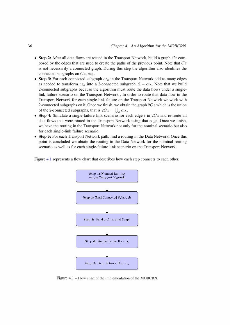
Figure 4.1 represents a flow chart that describes how each step connects to each other.
Figure 4.1 – Flow chart of the implementation of the MOBCRN.

4.2. Algorithm Description 37
Now that we have described the algorithm from a high level perspective we proceed toexplain each step in detail.
4.2.2 Low Level Description
4.2.2.1 Step 1: Nominal Routing on the Transport Network
This part of the algorithm finds a nominal routing scenario on the Transport Network foreach data flow defined on the Data Network. In order to route the data flows in the TransportNetwork the algorithm must find the terminal nodes of the Transport Network. A terminalnode is just a Transport Network node that generates o terminates a data flow in the TransportNetwork.
Traffic flows are generated and terminated at the Data Network. However, the Data Networkuses the services provided by the Transport Network to carry the information from one side toanother. In order to achieve that, Data Network nodes that generates traffic delivers that traffic toa Transport Network node. That node is, from the Transport Network perspective, the one thatgenerates the traffic, so it is a terminal node. In the same way the last transport node delivers thedata to the Data Network node which effectively terminates the flow. However, that transportnode is, from the Transport Network perspective, the one that terminates the traffic, so it is alsoa terminal node. Terminal and data nodes that generates and terminates traffic are related bythe tns function. An example of this situation is showed in Figure 4.2.
tns
Data Network
Transport Network
Terminal node
Traffic flow
Transport route
v1v2
v3
v4v5
tns(v1)t2
t3
tns(v4)t5
t6t7
t8
Figure 4.2 – Transport Network with terminal nodes.
38 Chapter 4. An Algorithm for the MOBCRN
After we have identified the terminal nodes we proceed to find a nominal routing scenario.This is, to select the Transport Network links that are going to be used to route the traffic flowswhen all transport links are active. The following aspects must be considered in order to selectthese links:
Length of the routes. As we explained before, the routing cost depends linearly on thelength of the routes. Thus, finding the shortest path for each route is critical in order to achievethe goal of minimizing the routing cost. In order to achieve this the algorithm not only seeksfor the shortest path on the existing transport links but also searches for the possibility ofinstalling additional transport links. If the shortest path is achieved installing additional trans-port links and the cost of installing them fits within the available installation budget I , thenthese new links are added to the network. Otherwise, the shortest path is searched within theoriginal Transport Network. The set of nodes and edges that builds the shortest path for eachtraffic flow will be called the Minimum Cost Transport Network, (MCTN). Our shortest pathalgorithm (hereafter SPA), based on Dijkstra’s implementation [19], is described in detail insection 4.2.2.6.
This scenario adds some complexity to the problem. In case that the MCTN is achievedinstalling additional links whose total installation cost exceeds the installation budget, the al-gorithm must decide which links to drop from that network in order to achieve the minimumcost constrained according to I .
In addition to that, the algorithm must take special care of the possibility of re-using links
for more than one traffic flow. This is because of how the Transport Network works. Once wehave assigned a capacity on a transport link that capacity is statically reserved on the link, nomatter the portion of the capacity that is effectively used by the traffic flow. This scenario isillustrated in the following example.
4.2. Algorithm Description 39
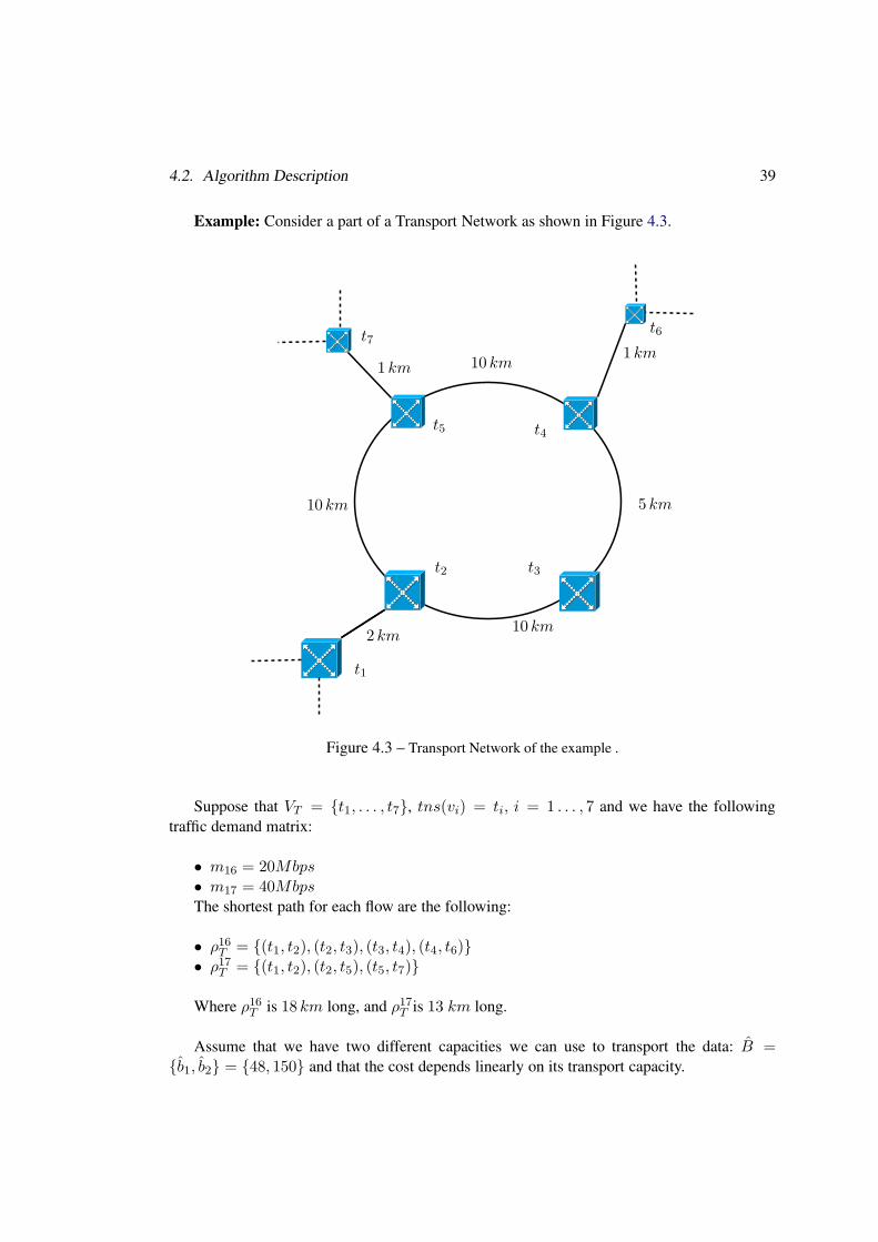
Example: Consider a part of a Transport Network as shown in Figure 4.3.
10 km
10 km
10 km
1 km1 km
2 km
5 km
t1
t2 t3
t4t5
t6t7
Figure 4.3 – Transport Network of the example .
Suppose that VT = {t1, . . . , t7}, tns(vi) = ti, i = 1 . . . , 7 and we have the followingtraffic demand matrix:
• m16 = 20Mbps• m17 = 40MbpsThe shortest path for each flow are the following:
• ρ16T = {(t1, t2), (t2, t3), (t3, t4), (t4, t6)}• ρ17T = {(t1, t2), (t2, t5), (t5, t7)}
Where ρ16T is 18 km long, and ρ17T is 13 km long.
Assume that we have two different capacities we can use to transport the data: B ={b1, b2} = {48, 150} and that the cost depends linearly on its transport capacity.
40 Chapter 4. An Algorithm for the MOBCRN
The assigned capacity for the data links B is:• b12 = 150• b23 = 48• b34 = 48• b46 = 48• b25 = 48• b57 = 48The technology cost function T is:• T (b1) = 10• T (b2) = 30Then we have the following routing costs:• cost(ρ16T , T (B)) = 30× 2 + 10× (10 + 5 + 1) = 220• cost(ρ17T , T (B)) = 30× 2 + 10× (10 + 1) = 170
Despite we have that cost(ρ16T , T (B)) = 220 and cost(ρ17T , T (B)) = 170 the total costis not 390. This is because the first link that is used in the routing, {t1, t2}, is shared betweenboth flows. As the link is used by the first flow, the cost of using that link for the second flowis 0. Thus the total cost for the routing is 330.
Number of edges to be used. In our problem, we must find a routing for each single-linkfailure scenario. Thus, the less is the number of edges selected in the nominal routing scenariothe less is the number of failure scenarios that will need to be considered. Moreover, since thelarger the number of edges the larger the risk of experiencing a failure, the number of edgesused in the nominal scenario also impacts in the robustness of the network. For these tworeasons, in case that the algorithm finds more than one routing path with the same cost it willselect the one that contains the less number of edges.
4.2. Algorithm Description 41
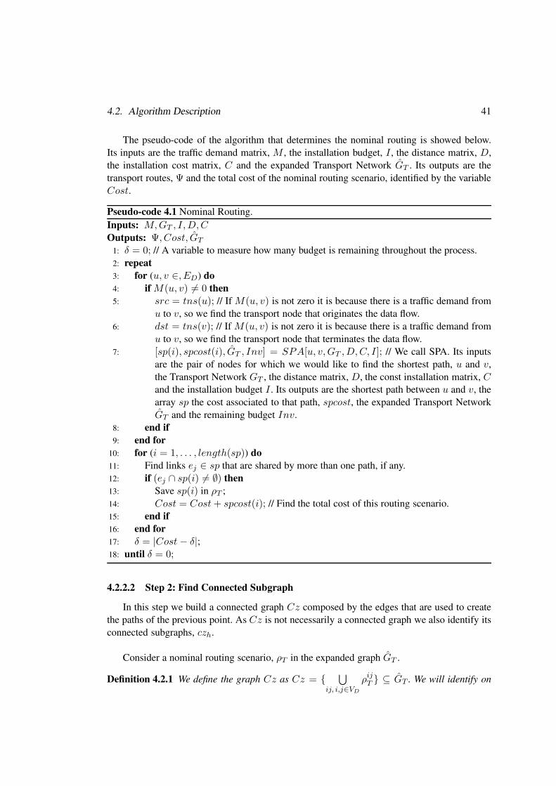
The pseudo-code of the algorithm that determines the nominal routing is showed below.Its inputs are the traffic demand matrix, M , the installation budget, I , the distance matrix, D,the installation cost matrix, C and the expanded Transport Network GT . Its outputs are thetransport routes, Ψ and the total cost of the nominal routing scenario, identified by the variableCost.
Pseudo-code 4.1 Nominal Routing.Inputs: M,GT , I,D,COutputs: Ψ, Cost, GT
1: δ = 0; // A variable to measure how many budget is remaining throughout the process.2: repeat
3: for (u, v ∈, ED) do
4: if M(u, v) 6= 0 then
5: src = tns(u); // If M(u, v) is not zero it is because there is a traffic demand fromu to v, so we find the transport node that originates the data flow.
6: dst = tns(v); // If M(u, v) is not zero it is because there is a traffic demand fromu to v, so we find the transport node that terminates the data flow.
7: [sp(i), spcost(i), GT , Inv] = SPA[u, v,GT ,D,C, I]; // We call SPA. Its inputsare the pair of nodes for which we would like to find the shortest path, u and v,the Transport Network GT , the distance matrix, D, the const installation matrix, Cand the installation budget I . Its outputs are the shortest path between u and v, thearray sp the cost associated to that path, spcost, the expanded Transport NetworkGT and the remaining budget Inv.
8: end if
9: end for
10: for (i = 1, . . . , length(sp)) do
11: Find links ej ∈ sp that are shared by more than one path, if any.12: if (ej ∩ sp(i) 6= ∅) then
13: Save sp(i) in ρT ;14: Cost = Cost+ spcost(i); // Find the total cost of this routing scenario.15: end if
16: end for
17: δ = |Cost− δ|;18: until δ = 0;
4.2.2.2 Step 2: Find Connected Subgraph
In this step we build a connected graph Cz composed by the edges that are used to createthe paths of the previous point. As Cz is not necessarily a connected graph we also identify itsconnected subgraphs, czh.
Consider a nominal routing scenario, ρT in the expanded graph GT .
Definition 4.2.1 We define the graph Cz as Cz = {⋃
ij, i,j∈VD
ρijT } ⊆ GT . We will identify on
42 Chapter 4. An Algorithm for the MOBCRN
Cz its 2-connex components and refer to its n-th component as czn.
This step of the algorithm not only identifies the connected subgraphs but also its degree-1nodes.
Definition 4.2.2 A transport node t of a connected subgraph czn is a degree-1 node if it satis-
fies the following conditions:
1. t is either tns(i) or tns(j), a terminal node of a transport routing ρijT , such that
ρijT ⊆ czn; i, j ∈ VD.
2. There is not another transport routing ρklT ⊆ czn; k, l ∈ VD such that t is not a terminal
node and {t ∩ ρklT } 6= ∅.
Let’s review the following example in order to clarify these ideas.
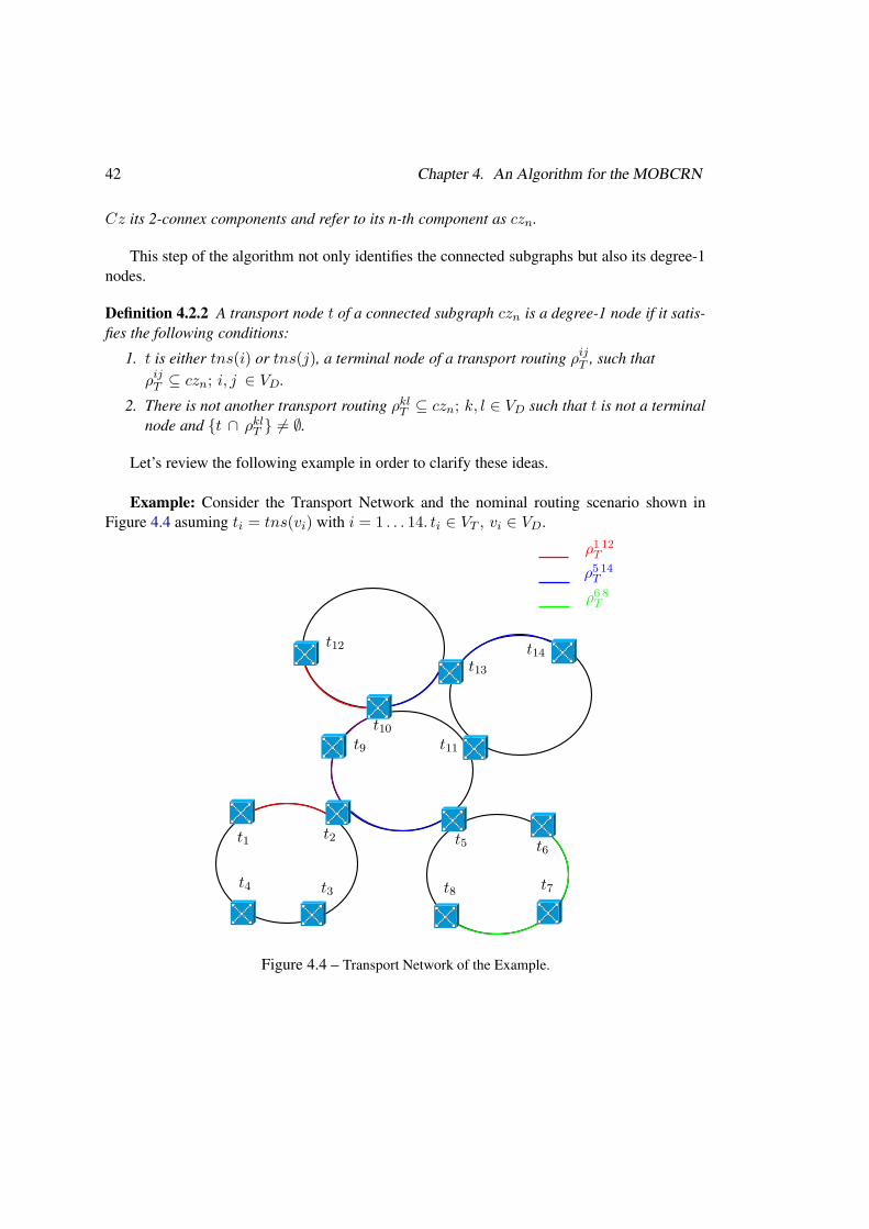
Example: Consider the Transport Network and the nominal routing scenario shown inFigure 4.4 asuming ti = tns(vi) with i = 1 . . . 14. ti ∈ VT , vi ∈ VD.
ρ1 12T
ρ5 14T
ρ6 8T
t1 t2
t3t4
t5 t6
t7t8
t9
t10t11
t12
t13t14
Figure 4.4 – Transport Network of the Example.
4.2. Algorithm Description 43
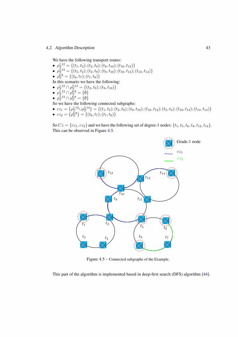
We have the following transport routes:• ρ1 12T = {(t1, t2); (t2, t9); (t9, t10); (t10, t12)}• ρ5 14T = {(t5, t2); (t2, t9); (t9, t10); (t10, t13); (t13, t14)}• ρ6 8T = {(t6, t7); (t7, t8)}In this scenario we have the following:• ρ1 12T ∩ ρ5 14T = {(t2, t9); (t9, t10)}• ρ1 12T ∩ ρ6 8T = {∅}• ρ5 14T ∩ ρ6 8T = {∅}So we have the following connected subgraphs:• cz1 = {ρ1 12T ∪ρ5 14T } = {(t1, t2); (t2, t9); (t9, t10); (t10, t12); (t5, t2); (t10, t13); (t13, t14)}• cz2 = {ρ6 8T } = {(t6, t7); (t7, t8)}
So Cz = {cz1, cz2} and we have the following set of degree-1 nodes: {t1, t5, t6, t8, t12, t14}.This can be observed in Figure 4.5.
cz1
cz2
Grade-1 node
t1 t2
t3t4
t5 t6
t7t8
t9
t10t11
t12t13
t14
Figure 4.5 – Connected subgraphs of the Example.
This part of the algorithm is implemented based in deep-first search (DFS) algorithm [44].
44 Chapter 4. An Algorithm for the MOBCRN
4.2.2.3 Step 3: Build 2-Connected Graph
Once the algorithm has identified the connected subgraphs, the next step is to build the2-connected graphs. As we explained in the previous subsection the connected subgraphs iden-tified are delimited by degree-1 nodes. A 2-connected graph is a connected subgraph in GT
whose nodes are connected at least by two edge-disjoint paths.
This step takes as inputs the connected subgraphs and its degree-1 nodes and adds links tothem in order to increase its connectivity degree at least by one.
One of the requirements of the problem is that the algorithm must find routes to every singlefailure scenario. Having degree-1 nodes in our solution will not satisfy that requirement. If thelink that connects a degree-1 node to the rest of the network fails, then it will be isolated fromthe rest of the Transport Network so the incoming or outgoing traffic from that node will notbe able to be routed.
Considering this, the goal of this step is to build 2-connected graphs so in case of a singlefailure scenario all the traffic routed within that connected subgraph can still be routed there.
For each degree-1 node t this step runs the SPA for t and any other transport node thatbelongs to a connected subgraph. In order to avoid selecting links that are already on the con-nected subgraphs these links are tagged with ∞ distance. When the algorithm finds the shortestpath between t and any other transport node that belongs to a connected subgraph it saves theone that has shortest length.
Once the algorithm iterates over all degree-1 nodes the 2-connected graphs are built. Thefollowing example illustrates this.
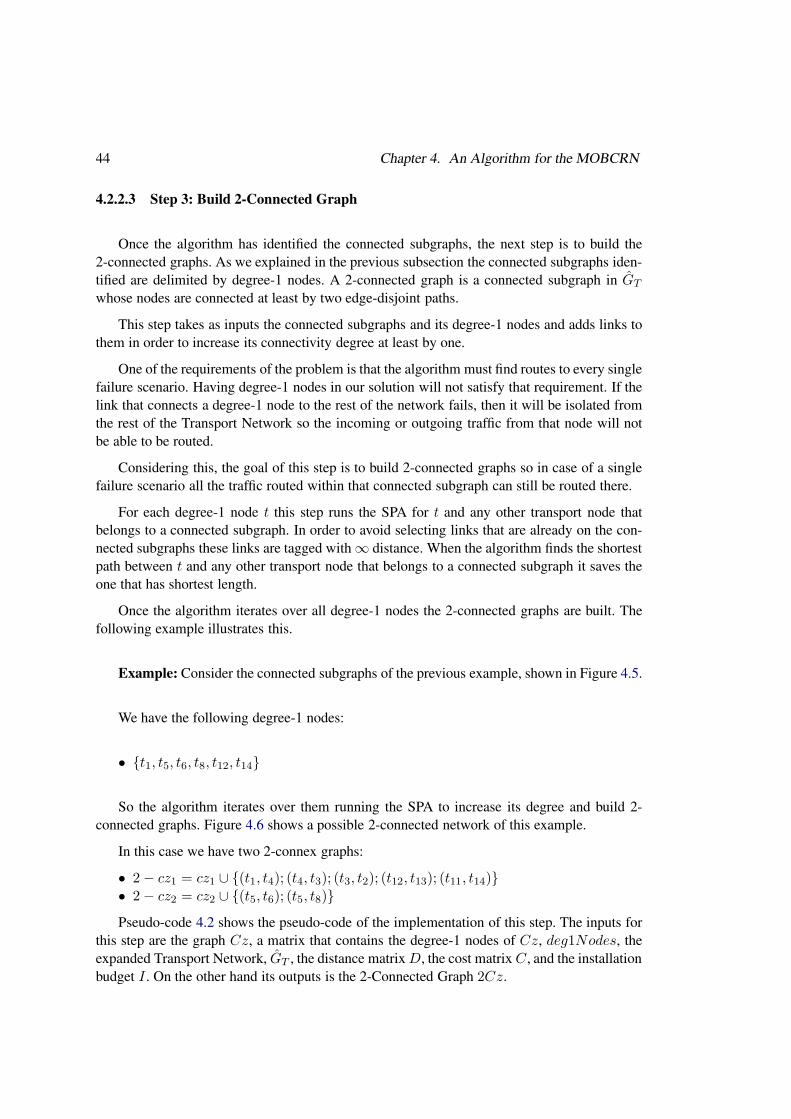
Example: Consider the connected subgraphs of the previous example, shown in Figure 4.5.
We have the following degree-1 nodes:
• {t1, t5, t6, t8, t12, t14}
So the algorithm iterates over them running the SPA to increase its degree and build 2-connected graphs. Figure 4.6 shows a possible 2-connected network of this example.
In this case we have two 2-connex graphs:
• 2− cz1 = cz1 ∪ {(t1, t4); (t4, t3); (t3, t2); (t12, t13); (t11, t14)}• 2− cz2 = cz2 ∪ {(t5, t6); (t5, t8)}
Pseudo-code 4.2 shows the pseudo-code of the implementation of this step. The inputs forthis step are the graph Cz, a matrix that contains the degree-1 nodes of Cz, deg1Nodes, theexpanded Transport Network, GT , the distance matrix D, the cost matrix C , and the installationbudget I . On the other hand its outputs is the 2-Connected Graph 2Cz.
4.2. Algorithm Description 45
2− cz1
2− cz2
t1 t2
t3t4
t5 t6
t7t8
t9t10
t11
t12t13
t14
Figure 4.6 – 2-connected graphs of the Example.
Pseudo-code 4.2 Build 2-Connected Graph.
Inputs: Cz, deg1Nodes, GT , D, C , I .Outputs: 2Cz
1: for (All edges e in Cz) do
2: C(e) = ∞; // Set the cost of the edges of the connected subgraphs to ∞ so the SPAwould not run over them.
3: end for
4: for (Each connected subgraph czh in Cz) do
5: for (Each degree-1 node i in czh) do
6: for (Each node j in czh) do
7: [sp(i), spcost(i), GT , Inv] = SPA[i, j,GT ,D,C, I];// For each degree-1 node call the SPA to find the shortest path to every node j inczh.
8: end for
9: Add min(sp(i)) to the connected subgraph to build the 2-Connected Graph, 2Cz.10: end for
11: end for
In order to construct the 2-connex graph we could also have used algotithms such as [15,43, 45]. However, our solution using the SPA performed accordingly when we executed thealgorithm in the scenarios we run.

46 Chapter 4. An Algorithm for the MOBCRN
4.2.2.4 Step 4: Simple Failure Routing
An important criteria considered to design the Transport Network is that it must be tolerantto single-link failures. In this step we simulate a single-link failure for each link that is part ofthe 2-connected graph. In order to simulate the failure, the algorithm sets the length of the linkto infinite. After that, it looks for the data flows that are transported by that link and re-routethem within the 2-connected graph using the SPA.
Once the iteration over all links that belongs to the 2-connected graph the simulation isfinished, having all the single-link failure routing scenarios.
The following example illustrates this.
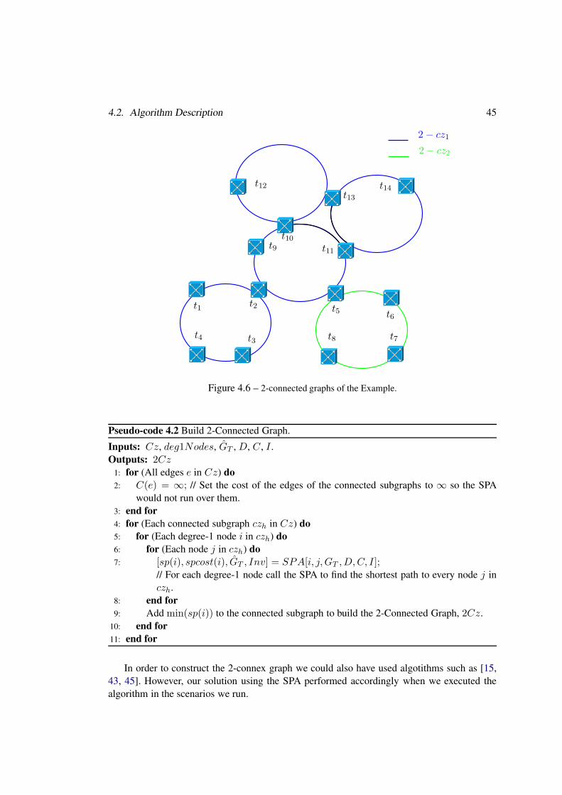
Example: Consider the 2-connected graph of the previous example and the following in-formation
Suppose we have the following traffic demand matrix:
• m1 12 = 200Mbps• m3 10 = 600Mbps
Suppose that given the technology and link-length information the shortest path given bythe SPA for each flow are the following:
• ρ1 12T = {(t1, t2); (t2, t9); (t9, t10); (t10, t12)}• ρ3 10T = {(t3, t2); (t2, t9); (t9, t10)}
These routes are showed in dotted lines in Figure 4.7.
4.2. Algorithm Description 47
2− cz1
2− cz2
ρ3 10T
ρ1 12T
t1 t2
t3t4
t5 t6
t7t8
t9
t10
t11
t12t13
t14
Figure 4.7 – Transport routes in the 2-connected graph.
Now suppose that link e = (t2, t9) fails. In that case both routes are affected so they mustbe re-routed to transport the data flows in that scenario. A possible routing in that failure sce-nario is the following:
• ρ1 12Te = {(t1, t2); (t2, t5); (t5, t11); (t11, t14); (t14, t13); (t13, t10); (t10, t12)}• ρ3 10Te = {(t3, t2); (t2, t5); (t5, t11); (t11, t14); (t14, t13); (t13, t10)}
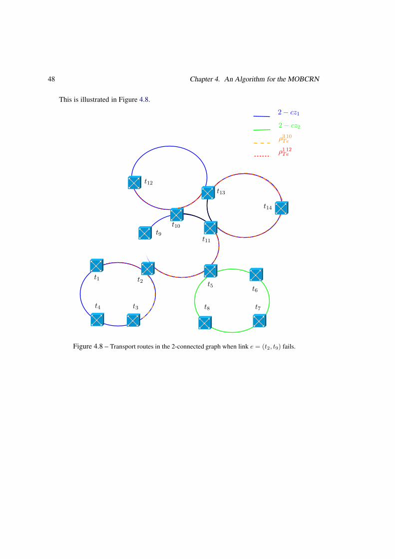
48 Chapter 4. An Algorithm for the MOBCRN
This is illustrated in Figure 4.8.
2− cz1
2− cz2
ρ3 10Te
ρ1 12Te
t1 t2
t3t4
t5 t6
t7t8
t9
t10
t11
t12t13
t14
Figure 4.8 – Transport routes in the 2-connected graph when link e = (t2, t9) fails.
4.2. Algorithm Description 49
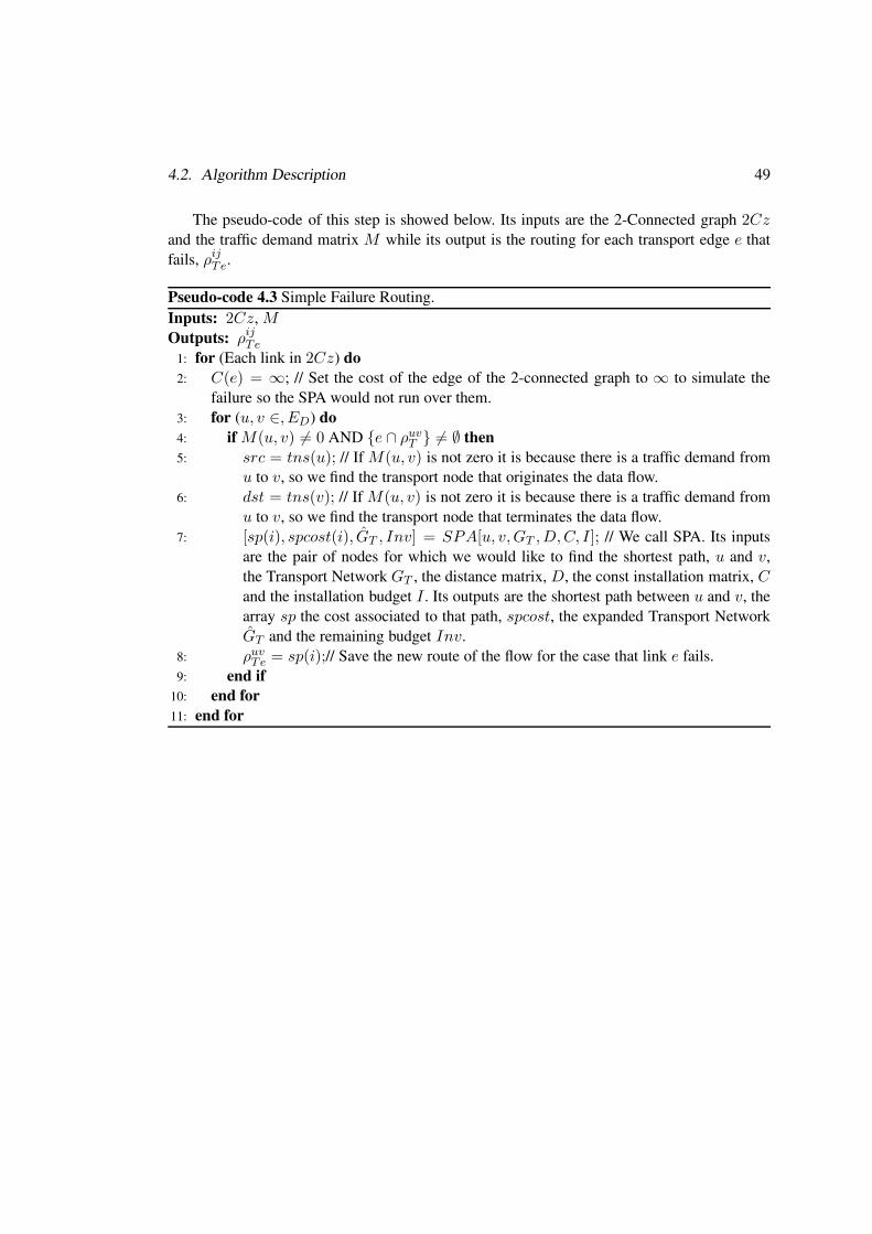
The pseudo-code of this step is showed below. Its inputs are the 2-Connected graph 2Czand the traffic demand matrix M while its output is the routing for each transport edge e thatfails, ρijT e.
Pseudo-code 4.3 Simple Failure Routing.Inputs: 2Cz, MOutputs: ρijT e
1: for (Each link in 2Cz) do
2: C(e) = ∞; // Set the cost of the edge of the 2-connected graph to ∞ to simulate thefailure so the SPA would not run over them.
3: for (u, v ∈, ED) do
4: if M(u, v) 6= 0 AND {e ∩ ρuvT } 6= ∅ then
5: src = tns(u); // If M(u, v) is not zero it is because there is a traffic demand fromu to v, so we find the transport node that originates the data flow.
6: dst = tns(v); // If M(u, v) is not zero it is because there is a traffic demand fromu to v, so we find the transport node that terminates the data flow.
7: [sp(i), spcost(i), GT , Inv] = SPA[u, v,GT ,D,C, I]; // We call SPA. Its inputsare the pair of nodes for which we would like to find the shortest path, u and v,the Transport Network GT , the distance matrix, D, the const installation matrix, Cand the installation budget I . Its outputs are the shortest path between u and v, thearray sp the cost associated to that path, spcost, the expanded Transport NetworkGT and the remaining budget Inv.
8: ρuvTe = sp(i);// Save the new route of the flow for the case that link e fails.9: end if
10: end for
11: end for
50 Chapter 4. An Algorithm for the MOBCRN
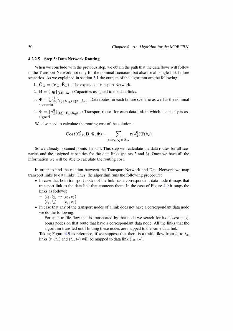
4.2.2.5 Step 5: Data Network Routing
When we conclude with the previous step, we obtain the path that the data flows will followin the Transport Network not only for the nominal scenaraio but also for all single-link failurescenarios. As we explained in section 3.1 the outputs of the algorithm are the following:
1. GT = (VT, ET) : The expanded Transport Network.
2. B = {bij}(i,j)∈ED: Capacities assigned to the data links.
3. Φ = {ρijDt}i,j∈VD,t∈{∅∪ET} : Data routes for each failure scenario as well as the nominal
scenario.
4. Ψ = {ρijT}(i,j)∈ED,bij 6=0 : Transport routes for each data link in which a capacity is as-signed.
We also need to calculate the routing cost of the solution:
Cost(GT,B,Φ,Ψ) =∑
e=(vi,vj)∈ED
r(ρijT)T(be)
So we already obtained points 1 and 4. This step will calculate the data routes for all sce-narios and the assigned capacities for the data links (points 2 and 3). Once we have all theinformation we will be able to calculate the routing cost.
In order to find the relation between the Transport Network and Data Network we maptransport links to data links. Thus, the algorithm runs the following procedure:
• In case that both transport nodes of the link has a correspondant data node it maps thattransport link to the data link that connects them. In the case of Figure 4.9 it maps thelinks as follows:− (t1, t2) → (v1, v2)− (t1, t3) → (v1, v3)
• In case that any of the transport nodes of a link does not have a correspondant data nodewe do the following:− For each traffic flow that is transported by that node we search for its closest neig-
bours nodes on that route that have a correspondant data node. All the links that thealgorithm transited until finding these nodes are mapped to the same data link.
Taking Figure 4.9 as reference, if we suppose that there is a traffic flow from t3 to t2,links (t3, t4) and (t4, t2) will be mapped to data link (v3, v2).
4.2. Algorithm Description 51
Data Network
Transport Network
tns
v1
v2
v3
t1t2t3
t4
Figure 4.9 – Network of the example.
After doing this, the algorithm calculates the assigned capacities for each data link. Thisis performed calculating the summatory of the traffic that is being transported by the transportlinks that are mapped into them. As in each routing scenario the traffic that is being transportedby the transport links varies, the algorithm must choose the scenario in which the transport linktransports the largest traffic.
The following example illustrates this.
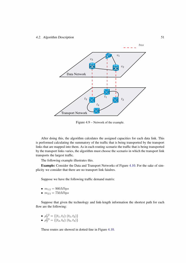
Example: Consider the Data and Transport Networks of Figure 4.10. For the sake of sim-plicity we consider that there are no transport link faiulres.
Suppose we have the following traffic demand matrix:
• m1 2 = 900Mbps• m2 3 = 750Mbps
Suppose that given the technology and link-length information the shortest path for eachflow are the following:
• ρ1 2T = {(t1, t5); (t5, t2)}• ρ2 3T = {(t2, t6); (t6, t3)}
These routes are showed in dotted-line in Figure 4.10.

52 Chapter 4. An Algorithm for the MOBCRN
Data Network
Transport Network
tns
ρ1 2T
ρ2 3T
v1
v2
v3
t1
t2
t3
t4t5
t6
Figure 4.10 – Data and Transport Network of the example.
In this case we have the following mapping:
• {(t1, t5), (t5, t2)} → (v1, v2)• {(t2, t6), (t6, t3)} → (v2, v3)
Suppose we have the following available capacities to assign in the Data Network:
• 1Gbps• 10Gbps
4.2. Algorithm Description 53
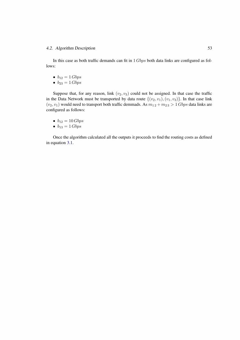
In this case as both traffic demands can fit in 1Gbps both data links are configured as fol-lows:
• b12 = 1Gbps• b23 = 1Gbps
Suppose that, for any reason, link (v2, v3) could not be assigned. In that case the trafficin the Data Network must be transported by data route {(v2, v1), (v1, v3)}. In that case link(v2, v1) would need to transport both traffic demmads. As m1 2+m2 3 > 1Gbps data links areconfigured as follows:
• b12 = 10Gbps• b13 = 1Gbps
Once the algorithm calculated all the outputs it proceeds to find the routing costs as definedin equation 3.1.
54 Chapter 4. An Algorithm for the MOBCRN
The pseudo-code of this step is showed below. The inputs are the 2-Connected Network,2Cz and the traffic demand matrix M . On the other hand the outputs are the capacities assignedto the data links, B, and the data routes for each failure scenario as well as the nominal scenarioΦ.
Pseudo-code 4.4 Data Network Routing.Inputs: 2Cz,MOutputs: B,Φ
1: Find the Data Network links to be used:
2: for (t = (ti, tj) ∈ 2Cz) do
3: for (u, v ∈, ED) do
4: if M(u, v) 6= 0 then
5: Find the closest neighbours of ti and tj , ni and nj in the flow originated in tns(u)and terminated in tns(v) such that ni and nj have va and vb as correspondant nodesin the Data Network respectively;
6: Map the path {n(i), . . . , n(j)} to (va, vb) ∈ ED;7: Set capab = 0; // Set the initial capacity of the data link to 0.8: if (va, vb) /∈ S then
9: Add (va, vb) to a set of data links S;10: else
11: EXIT; // If two neighbours can only be mapped to the same couple of data nodesthe algorithm exits as there is not feasible solution. This is explained deeply inSection 4.2.3.
12: end if
13: Construct ρuvDt;
14: Add ρuvDtto Φ;
15: end if
16: end for
17: end for
18: Calculate the capacities for the data links:
19: for (e ∈ S) do
20: for (Each routing scenario) do
21: if (ρuvT ∩ e) 6= ∅ then
22: Add the capacity of (u, v) to capTemp(e); // capTemp is a vector used to storethe capacities temporarily.
23: end if
24: cap(e) = max(cap(e), capTemp(e));25: capTemp(e) = 0;26: end for
27: Set b(e) as the minimum available capacity that transports cap(e);28: end for
4.2. Algorithm Description 55
4.2.2.6 Shortest Path Algorithm
This function implements an heuristic based on Dijkstra’s shortest path algorithm [19] thatfinds the shortest path between two nodes of the Transport Network. Its inputs are the follow-ing:
• Source and destination nodes.• Transport Network GT .• Distance matrix D.• Installation costs matrix C .• Installation budget I .
The outputs of the SPA are the following:
• The shortest path between source and destination nodes and its associated cost.• The modified Transport Network GT .• The updated installation budget Inv.
Note that the Transport Network can be either modified or not. This depends on the Trans-port Network, the length and costs of the potential links to be added and the installation budget.In case that the SPA finds a shortest path adding some new links whose installation cost is lowerthan the budget then the Transport Network is modified.
The core of the SPA is based on the same idea that uses the well known Djkstra’s algorithm[19]. The big difference is that, for each transport node, the SPA searches not only the realneighbours but also all potential ones. A transport node t is a potential neighbour of a transportnode v if the installation cost of the link that connects them is smaller than the available instal-lation budget. So, the SPA checks that condition for each node when calculating the shortestpath. In case that a link is installed the installation budget is updated to reflect the installationof that link.

56 Chapter 4. An Algorithm for the MOBCRN
The pseudo-code of the SPA is showed below. Its inputs are the pair of nodes for whichwe would like to find the shortest path, src and dst, the Transport Network GT , the distancematrix, D, the const installation matrix, C and the installation budget I . Its outputs are theshortest path between src and dst, the array sp, the cost associated to that path, spcost, theexpanded Transport Network GT and the remaining budget Inv.
Pseudo-code 4.5 Shortest Path Algorithm.Inputs: src, dst, GT , D, C , I .Outputs: sp, spcost, GT , Inv.
1: dist(u) = ∞ ∀u ∈ VT \ {src}; // Set the distance between the source and the rest ofthe nodes to ∞.
2: dist(src) = 0; // Set the distance from src to src to 0.3: visited(u) = 0 ∀u ∈ VT ; // Array of visited nodes.4: while (sum(visited) 6= |VT |) do
5: u = argmin{dist(i) : i ∈ VT , visited(i) = 0};6: visited(u) = 1; // Mark the node as visited.7: for (i = 1 : |VT |) do
8: if (dist(u) +D(u, i) < dist(i)) then
9: if ((u, i) ∈ ET ) then
10: dist(i) = dist(u) +D(u, i); // Update the distance.11: prev(i) = u; // Set u as the previous node.12: else if (C(u, i) ≤ I) then
13: dist(i) = dist(u) +D(u, i); // Update the distance.14: prev(i) = u; // Set u as the previous node.15: I = I − C(u, i); // Update the budget.16: ET = ET ∪ {(u, i)}; // Add the new edge to GT .17: end if
18: end if
19: end for
20: end while
21: sp = [dst]; // The shortest path array.22: while (sp(1) 6= src) do
23: sp = [prev(sp(1)), sp]; // Build the shortest path array.24: end while
25: spCost = dist(dst);// Calculate the distance from src to dst.
4.2. Algorithm Description 57
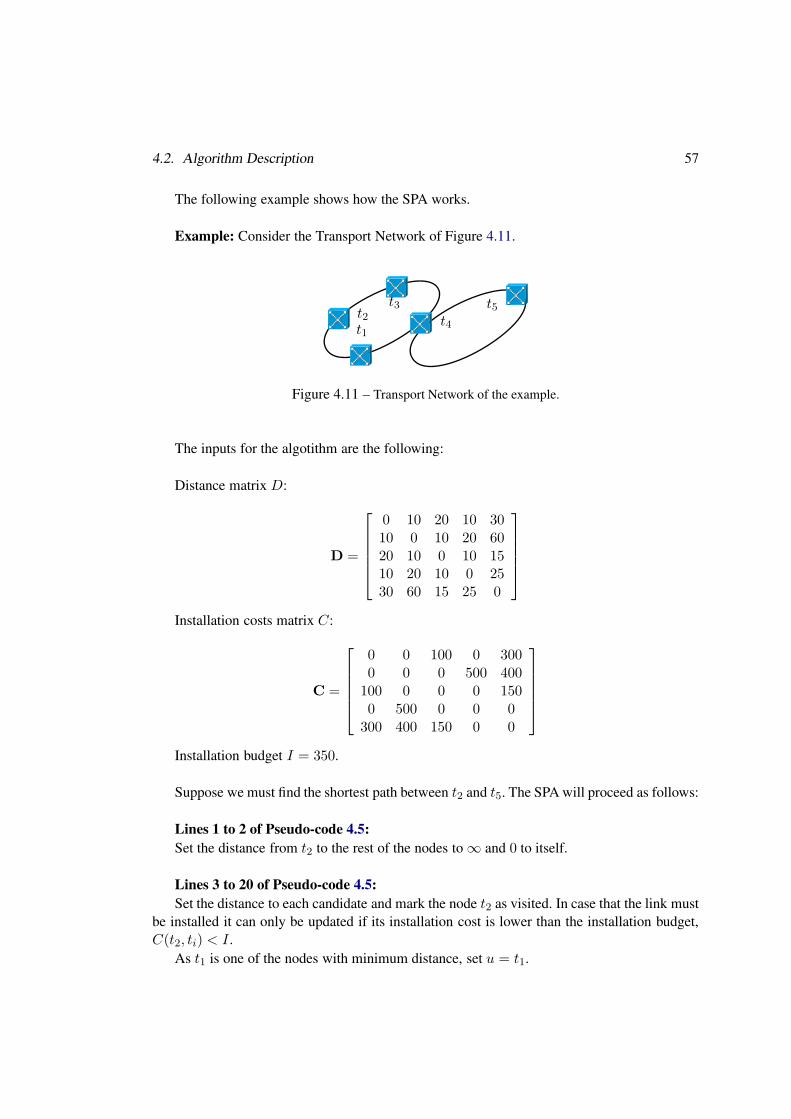
The following example shows how the SPA works.
Example: Consider the Transport Network of Figure 4.11.
t1
t2t3
t4
t5
Figure 4.11 – Transport Network of the example.
The inputs for the algotithm are the following:
Distance matrix D:
D =
0 10 20 10 3010 0 10 20 6020 10 0 10 1510 20 10 0 2530 60 15 25 0
Installation costs matrix C:
C =
0 0 100 0 3000 0 0 500 400
100 0 0 0 1500 500 0 0 0
300 400 150 0 0
Installation budget I = 350.
Suppose we must find the shortest path between t2 and t5. The SPA will proceed as follows:
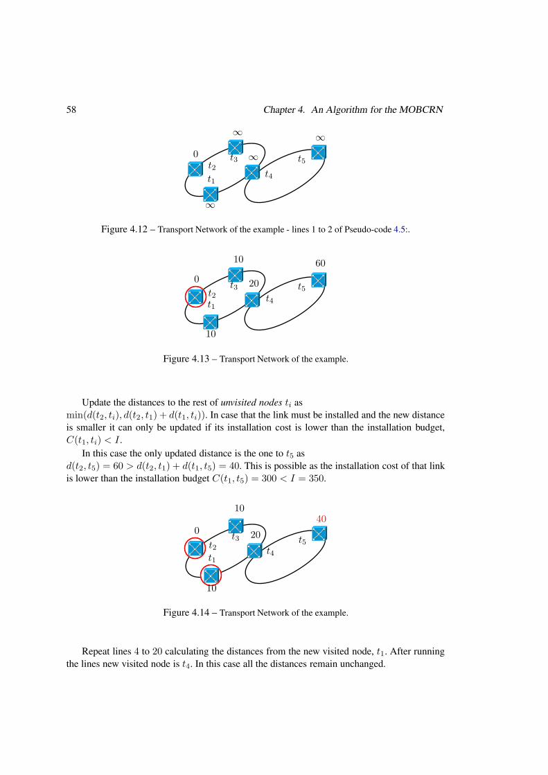
Lines 1 to 2 of Pseudo-code 4.5:
Set the distance from t2 to the rest of the nodes to ∞ and 0 to itself.
Lines 3 to 20 of Pseudo-code 4.5:
Set the distance to each candidate and mark the node t2 as visited. In case that the link mustbe installed it can only be updated if its installation cost is lower than the installation budget,C(t2, ti) < I .
As t1 is one of the nodes with minimum distance, set u = t1.
58 Chapter 4. An Algorithm for the MOBCRN
t1
t2t3
t4
t5∞
∞∞
∞
0
Figure 4.12 – Transport Network of the example - lines 1 to 2 of Pseudo-code 4.5:.
t1
t2t3
t4
t50
10
10
20
60
Figure 4.13 – Transport Network of the example.
Update the distances to the rest of unvisited nodes ti asmin(d(t2, ti), d(t2, t1) + d(t1, ti)). In case that the link must be installed and the new distanceis smaller it can only be updated if its installation cost is lower than the installation budget,C(t1, ti) < I .
In this case the only updated distance is the one to t5 asd(t2, t5) = 60 > d(t2, t1) + d(t1, t5) = 40. This is possible as the installation cost of that linkis lower than the installation budget C(t1, t5) = 300 < I = 350.
t1
t2t3
t4
t50
10
10
20
40
Figure 4.14 – Transport Network of the example.
Repeat lines 4 to 20 calculating the distances from the new visited node, t1. After runningthe lines new visited node is t4. In this case all the distances remain unchanged.
4.2. Algorithm Description 59
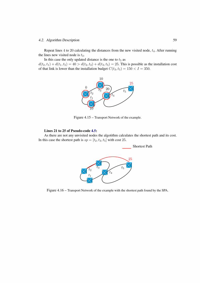
Repeat lines 4 to 20 calculating the distances from the new visited node, t4. After runningthe lines new visited node is t3.
In this case the only updated distance is the one to t5 asd(t2, t1) + d(t1, t5) = 40 > d(t2, t3) + d(t3, t5) = 25. This is possible as the installation costof that link is lower than the installation budget C(t3, t5) = 150 < I = 350.
t1
t2t3
t4
t50
10
10
20
25
Figure 4.15 – Transport Network of the example.
Lines 21 to 25 of Pseudo-code 4.5:
As there are not any unvisited nodes the algotithm calculates the shortest path and its cost.In this case the shortest path is sp = [t2, t3, t5] with cost 25.
t1
t2t3
t4
t5
Shortest Path
25
Figure 4.16 – Transport Network of the example with the shortest path found by the SPA.
60 Chapter 4. An Algorithm for the MOBCRN
4.2.3 Unfeasible Scenarios
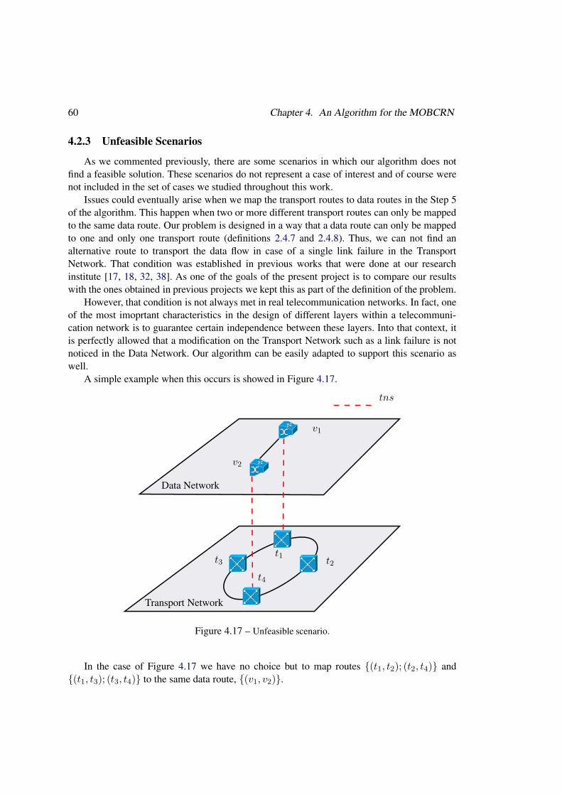
As we commented previously, there are some scenarios in which our algorithm does notfind a feasible solution. These scenarios do not represent a case of interest and of course werenot included in the set of cases we studied throughout this work.
Issues could eventually arise when we map the transport routes to data routes in the Step 5of the algorithm. This happen when two or more different transport routes can only be mappedto the same data route. Our problem is designed in a way that a data route can only be mappedto one and only one transport route (definitions 2.4.7 and 2.4.8). Thus, we can not find analternative route to transport the data flow in case of a single link failure in the TransportNetwork. That condition was established in previous works that were done at our researchinstitute [17, 18, 32, 38]. As one of the goals of the present project is to compare our resultswith the ones obtained in previous projects we kept this as part of the definition of the problem.
However, that condition is not always met in real telecommunication networks. In fact, oneof the most imoprtant characteristics in the design of different layers within a telecommuni-cation network is to guarantee certain independence between these layers. Into that context, itis perfectly allowed that a modification on the Transport Network such as a link failure is notnoticed in the Data Network. Our algorithm can be easily adapted to support this scenario aswell.
A simple example when this occurs is showed in Figure 4.17.
Data Network
Transport Network
tns
v1
v2
t1t2t3
t4
Figure 4.17 – Unfeasible scenario.
In the case of Figure 4.17 we have no choice but to map routes {(t1, t2); (t2, t4)} and{(t1, t3); (t3, t4)} to the same data route, {(v1, v2)}.

Part IV
RESULTS
61

Chapter 5
Test Cases Description
In this chapter we explain the test cases designed for which we run the algorithm. We dividethe test cases into two different sets. The first set of test cases intends to validate the developedalgorithm and compare its performance against other techniques to solve this kind of problems.
On the other hand, the second set of test cases are proposed to evaluate all functionalitiesof the algorithm. This is, the possibility of installing new transport links with some installationbudget constrains.
Both test cases are generated using the information provided by ANTEL from their Dataand Transport Network. This is an added value of this project as it is extremely interesting torun our algorithm using data from a real network such as ANTEL’s. This clearly shows howthis kind of techniques can be applied to help solving problems from real networks.
5.1 First Set of Test Cases
The test cases were defined during a project carried out by researchers from the Univer-sity of the Republic and ANTEL. They describe different situations and realities of ANTEL,considering several parameters that are under their control [38].
We choose this set of test cases because a couple of projects already worked on them [32,38]. Thus, by adjusting some inputs, it is possible to compare the performance of our algorithmwith other ways of solving this kind of problems such as using meta-heuristics [38] or binayinteger programming models [32]. This can be easily achieved by setting the installation budgetto zero, so there would not be any possibility of installing additional links in the TransportNetwork.
5.1.1 Problem Data
This section describes the inputs to the problem. As we said previously, all the data wasprovided by ANTEL:
• The Transport Network, including the nodes, edges and their lengths.• The available capacities B and their cost per kilometer, T : B → R
+0 .
63

64 Chapter 5. Test Cases Description
• The Data Network.
The topology of the Transport Network used to solve the problem is showed in Figure 5.1.
��� ���
��
��
������
���
��
��
��
���
���
��� �� ��� � ���
���
���
������
��
���
���
���
���
���
���
��
���
��
�� ���
��� ���
��� ���
� ���� ���
���
������ ���� �
�
� ��� ���
��� � ���� ���
��� ���
���
���
�� ��� ���
���
� � ���
�
���
�� ��
��
���
��� �� ��
��
������
��
���
��
��
���
���
��
��
���
�� ��� �� �� �� ���
���
������ ��� ��
���
���
���
���
���
���
���
���
���
���
���
�
���
���
Figure 5.1 – ANTEL’s Transport Network.
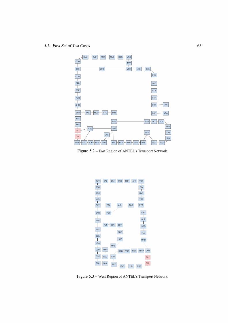
As this network is extremely big to make any useful calculation [32] it is divided in tworegions; the East Region and the West Region. By dividing the network in this way we stillmaintain the ring topology while generating two smaller networks. Both networks can be ob-served in Figure 5.2 and 5.3 respectively. It can be seen how nodes TIU and TIA appear in bothnetworks. The data nodes corresponding to each region were preserved along with the induceddata links.
5.1. First Set of Test Cases 65
���
���
��� ����� ��
��� ��
��
���
��� ��� ���
��
��� ��
���
���
��� ��
���
���
��� ��� ���
���
�����
���
��
���
��
���
���
���
���
���
��� ��� �� ��� ��� ���
���
��� �� ��� ���
���
���
���
���
��
���
���
���
���
���
Figure 5.2 – East Region of ANTEL’s Transport Network.
��� ���
��
��
������
���
��
��
��
���
���
��� �� ��� � ���
���
���
������
��
���
���
���
���
���
���
��
���
��
�� ���
��� ���
��� ���
� ���� ���
���
������ ���� �
�
� ��� ���
���
���
�
���
Figure 5.3 – West Region of ANTEL’s Transport Network.
66 Chapter 5. Test Cases Description
These regions are named east_copy and west_copy respectively.
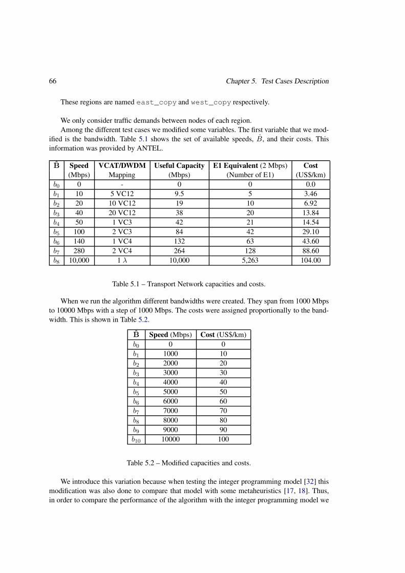
We only consider traffic demands between nodes of each region.Among the different test cases we modified some variables. The first variable that we mod-
ified is the bandwidth. Table 5.1 shows the set of available speeds, B, and their costs. Thisinformation was provided by ANTEL.
B Speed VCAT/DWDM Useful Capacity E1 Equivalent (2 Mbps) Cost
(Mbps) Mapping (Mbps) (Number of E1) (US$/km)b0 0 - 0 0 0.0b1 10 5 VC12 9.5 5 3.46b2 20 10 VC12 19 10 6.92b3 40 20 VC12 38 20 13.84b4 50 1 VC3 42 21 14.54b5 100 2 VC3 84 42 29.10b6 140 1 VC4 132 63 43.60b7 280 2 VC4 264 128 88.60b8 10,000 1 λ 10,000 5,263 104.00
Table 5.1 – Transport Network capacities and costs.
When we run the algorithm different bandwidths were created. They span from 1000 Mbpsto 10000 Mbps with a step of 1000 Mbps. The costs were assigned proportionally to the band-width. This is shown in Table 5.2.
B Speed (Mbps) Cost (US$/km)b0 0 0b1 1000 10b2 2000 20b3 3000 30b4 4000 40b5 5000 50b6 6000 60b7 7000 70b8 8000 80b9 9000 90b10 10000 100
Table 5.2 – Modified capacities and costs.
We introduce this variation because when testing the integer programming model [32] thismodification was also done to compare that model with some metaheuristics [17, 18]. Thus,in order to compare the performance of the algorithm with the integer programming model we

5.2. Performance Test Cases 67
must have the same set of test scenarios. The upper capacity, 10000 Mbps, was kept having asreference the capacity and cost information provided by ANTEL. The tests that introduce thischange in the set of bandwidths are identified by the word cap in their name.
Last but not least, we also modify the traffic demand. For this set of tests the traffic weightof the network was increased. Traffic demands were generated randomly and uniformly dis-tributed from 0 to 30000 Mbps. The number of nodes with traffic demand is half the number ofdata edges. The set of tests that includes this modification are identified by the word chargein their names, giving the notion that in these networks almost all edges will be designed andcharged, if possible, close to its maximum capacity.
5.2 Performance Test Cases
In this set of test cases we run the algorithm using the complete network, showed in Figure5.1. We run these test cases to test the algorithm in a big Transport Network with many datanodes exchanging data with each other while testing its potential to find new transport linksthat can transport the data flows more efficiently reducing the transport routing costs.
In order to let the algorithm evaluate the installation of new transport links we set thedistance of these new links as the one of a straight line that connects its endpoints. As we counton the geographical information for each transport node this can be done easily. This is shownin the following example.
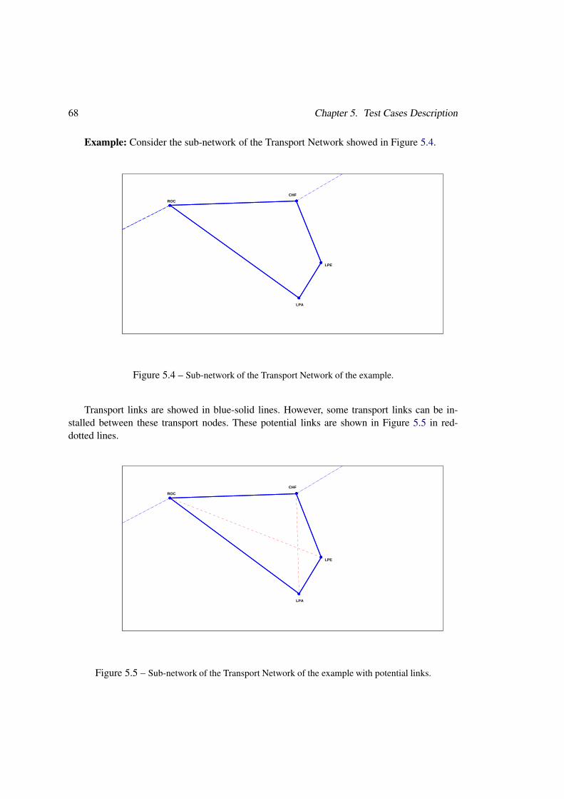
68 Chapter 5. Test Cases Description
Example: Consider the sub-network of the Transport Network showed in Figure 5.4.
CHF
LPE
LPA
ROC
Figure 5.4 – Sub-network of the Transport Network of the example.
Transport links are showed in blue-solid lines. However, some transport links can be in-stalled between these transport nodes. These potential links are shown in Figure 5.5 in red-dotted lines.
CHF
LPE
LPA
ROC
Figure 5.5 – Sub-network of the Transport Network of the example with potential links.
5.2. Performance Test Cases 69
For the sake of simplicity the installation cost will for each potential transport link is setas the same value of the distance between its endpoints. The installation budget is set as adistance value. For example, an installation budget of I = 1000 means that the algorithm caninstall additional transport links if and only if the length of the sum of all installed links isbelow 1000 km.
In this set of test cases we have all variables fixed but the installation budget. Thus, we willrun some examples varying that parameter and study the performance of the algorithm.

70 Chapter 5. Test Cases Description
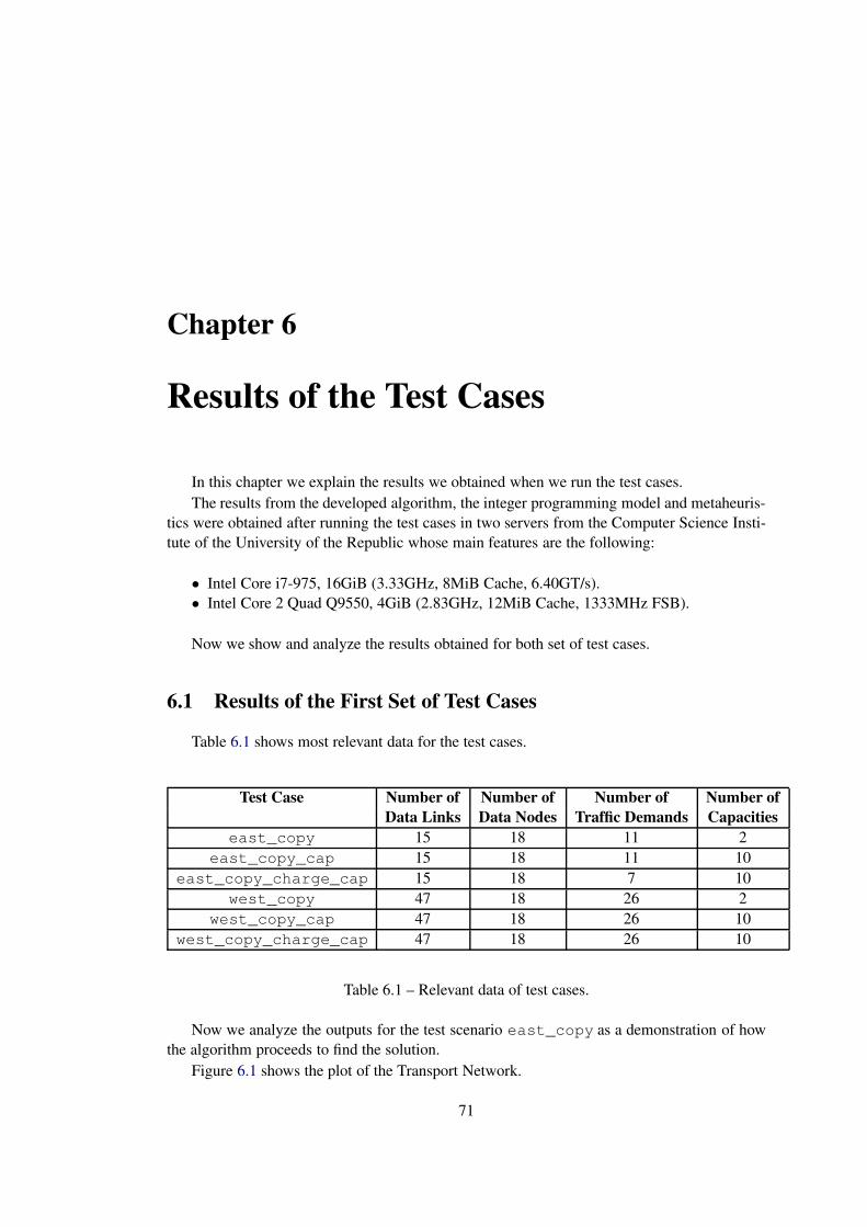
Chapter 6
Results of the Test Cases
In this chapter we explain the results we obtained when we run the test cases.The results from the developed algorithm, the integer programming model and metaheuris-
tics were obtained after running the test cases in two servers from the Computer Science Insti-tute of the University of the Republic whose main features are the following:
• Intel Core i7-975, 16GiB (3.33GHz, 8MiB Cache, 6.40GT/s).• Intel Core 2 Quad Q9550, 4GiB (2.83GHz, 12MiB Cache, 1333MHz FSB).
Now we show and analyze the results obtained for both set of test cases.
6.1 Results of the First Set of Test Cases
Table 6.1 shows most relevant data for the test cases.
Test Case Number of Number of Number of Number of
Data Links Data Nodes Traffic Demands Capacities
east_copy 15 18 11 2east_copy_cap 15 18 11 10
east_copy_charge_cap 15 18 7 10west_copy 47 18 26 2
west_copy_cap 47 18 26 10west_copy_charge_cap 47 18 26 10
Table 6.1 – Relevant data of test cases.
Now we analyze the outputs for the test scenario east_copy as a demonstration of howthe algorithm proceeds to find the solution.
Figure 6.1 shows the plot of the Transport Network.
71
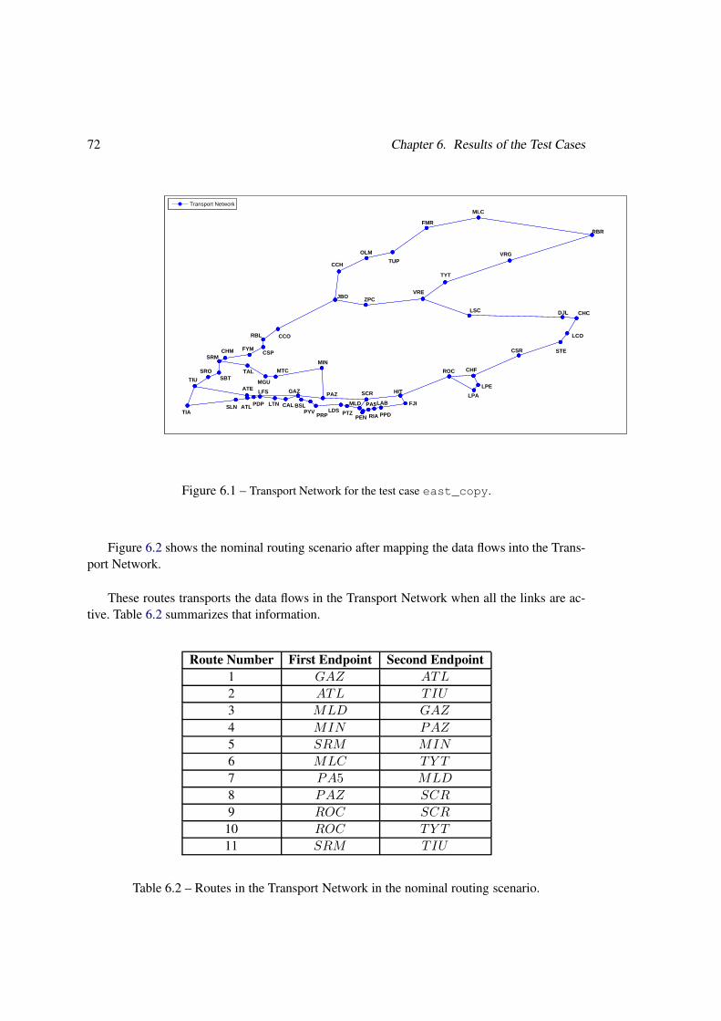
72 Chapter 6. Results of the Test Cases
SROSBT
SRMCHM FYM
CSP
RBL CCO
JBO
CCH
OLM
TUP
FMR
MLC
RBR
VRG
TYT
VRE
LSC DJL CHC
LCO
STECSR
CHF
LPE
LPA
ROC
HIT
FJI
PPD
LAB
RIA
PA5
PEN
MLD
PTZLDSPRP
PYVBSL
GAZ
CALLTN
LFS
PDPATLSLNTIA
TIU
ATE
TAL
MGU
MTC
MIN
PAZ SCR
ZPC
Transport Network
Figure 6.1 – Transport Network for the test case east_copy.
Figure 6.2 shows the nominal routing scenario after mapping the data flows into the Trans-port Network.
These routes transports the data flows in the Transport Network when all the links are ac-tive. Table 6.2 summarizes that information.
Route Number First Endpoint Second Endpoint
1 GAZ ATL
2 ATL TIU
3 MLD GAZ
4 MIN PAZ
5 SRM MIN
6 MLC TY T
7 PA5 MLD
8 PAZ SCR
9 ROC SCR
10 ROC TY T
11 SRM TIU
Table 6.2 – Routes in the Transport Network in the nominal routing scenario.
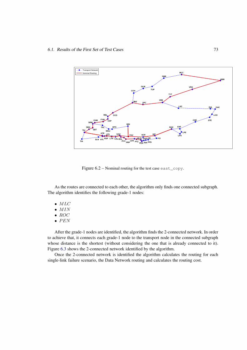
6.1. Results of the First Set of Test Cases 73
SROSBT
SRMCHM FYM
CSP
RBL CCO
JBO
CCH
OLM
TUP
FMR
MLC
RBR
VRG
TYT
VRE
LSC DJL CHC
LCO
STECSR
CHF
LPE
LPA
ROC
HIT
FJI
PPD
LAB
RIA
PA5
PEN
MLD
PTZLDSPRP
PYVBSL
GAZ
CALLTN
LFS
PDPATLSLNTIA
TIU
ATE
TAL
MGU
MTC
MIN
PAZ SCR
ZPC
Transport Network
Nominal Routing
Figure 6.2 – Nominal routing for the test case east_copy.
As the routes are connected to each other, the algorithm only finds one connected subgraph.The algorithm identifies the following grade-1 nodes:
• MLC• MIN• ROC• PEN
After the grade-1 nodes are identified, the algorithm finds the 2-connected network. In orderto achieve that, it connects each grade-1 node to the transport node in the connected subgraphwhose distance is the shortest (without considering the one that is already connected to it).Figure 6.3 shows the 2-connected network identified by the algorithm.
Once the 2-connected network is identified the algorithm calculates the routing for eachsingle-link failure scenario, the Data Network routing and calculates the routing cost.
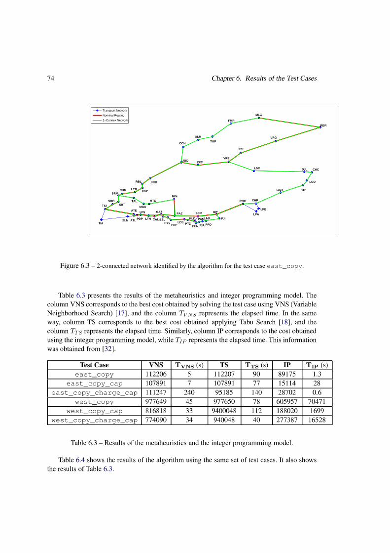
74 Chapter 6. Results of the Test Cases
SROSBT
SRMCHM FYM
CSP
RBL CCO
JBO
CCH
OLM
TUP
FMR
MLC
RBR
VRG
TYT
VRE
LSC DJL CHC
LCO
STECSR
CHF
LPE
LPA
ROC
HIT
FJI
PPD
LAB
RIA
PA5
PEN
MLD
PTZLDSPRP
PYVBSL
GAZ
CALLTN
LFS
PDPATLSLNTIA
TIU
ATE
TAL
MGU
MTC
MIN
PAZ SCR
ZPC
Transport Network
Nominal Routing
2−Connex Network
Figure 6.3 – 2-connected network identified by the algorithm for the test case east_copy.
Table 6.3 presents the results of the metaheuristics and integer programming model. Thecolumn VNS corresponds to the best cost obtained by solving the test case using VNS (VariableNeighborhood Search) [17], and the column TV NS represents the elapsed time. In the sameway, column TS corresponds to the best cost obtained applying Tabu Search [18], and thecolumn TTS represents the elapsed time. Similarly, column IP corresponds to the cost obtainedusing the integer programming model, while TIP represents the elapsed time. This informationwas obtained from [32].
Test Case VNS TVNS (s) TS TTS (s) IP TIP (s)east_copy 112206 5 112207 90 89175 1.3
east_copy_cap 107891 7 107891 77 15114 28east_copy_charge_cap 111247 240 95185 140 28702 0.6
west_copy 977649 45 977650 78 605957 70471west_copy_cap 816818 33 9400048 112 188020 1699
west_copy_charge_cap 774090 34 940048 40 277387 16528
Table 6.3 – Results of the metaheuristics and the integer programming model.
Table 6.4 shows the results of the algorithm using the same set of test cases. It also showsthe results of Table 6.3.
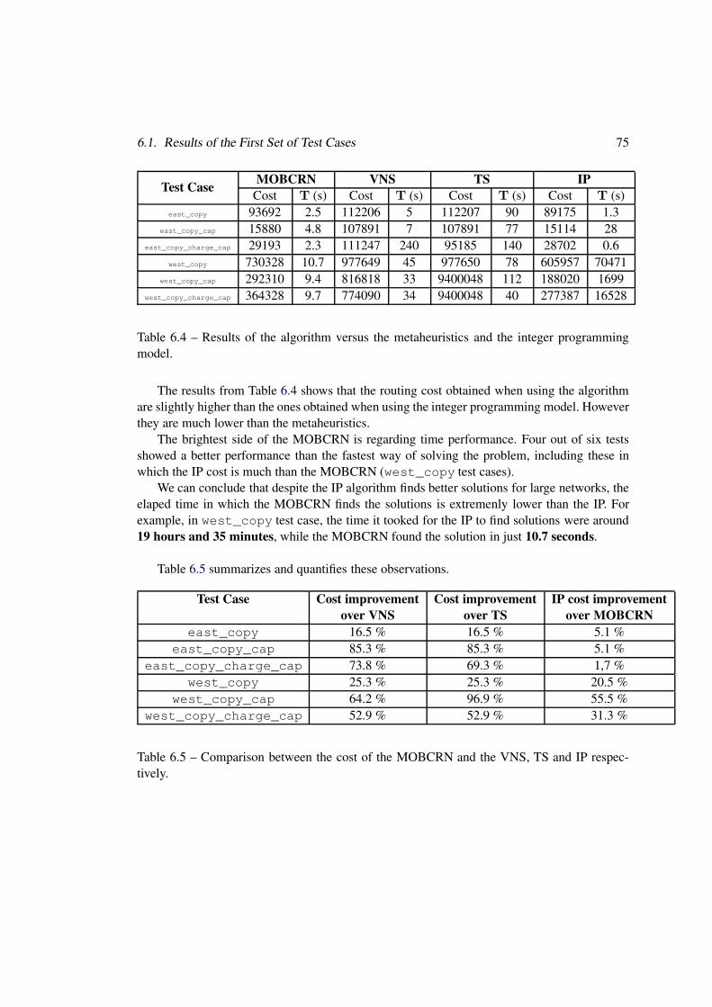
6.1. Results of the First Set of Test Cases 75
Test CaseMOBCRN VNS TS IP
Cost T (s) Cost T (s) Cost T (s) Cost T (s)east_copy 93692 2.5 112206 5 112207 90 89175 1.3
east_copy_cap 15880 4.8 107891 7 107891 77 15114 28east_copy_charge_cap 29193 2.3 111247 240 95185 140 28702 0.6
west_copy 730328 10.7 977649 45 977650 78 605957 70471west_copy_cap 292310 9.4 816818 33 9400048 112 188020 1699
west_copy_charge_cap 364328 9.7 774090 34 9400048 40 277387 16528
Table 6.4 – Results of the algorithm versus the metaheuristics and the integer programmingmodel.
The results from Table 6.4 shows that the routing cost obtained when using the algorithmare slightly higher than the ones obtained when using the integer programming model. Howeverthey are much lower than the metaheuristics.
The brightest side of the MOBCRN is regarding time performance. Four out of six testsshowed a better performance than the fastest way of solving the problem, including these inwhich the IP cost is much than the MOBCRN (west_copy test cases).
We can conclude that despite the IP algorithm finds better solutions for large networks, theelaped time in which the MOBCRN finds the solutions is extremenly lower than the IP. Forexample, in west_copy test case, the time it tooked for the IP to find solutions were around19 hours and 35 minutes, while the MOBCRN found the solution in just 10.7 seconds.
Table 6.5 summarizes and quantifies these observations.
Test Case Cost improvement Cost improvement IP cost improvement
over VNS over TS over MOBCRN
east_copy 16.5 % 16.5 % 5.1 %east_copy_cap 85.3 % 85.3 % 5.1 %
east_copy_charge_cap 73.8 % 69.3 % 1,7 %west_copy 25.3 % 25.3 % 20.5 %
west_copy_cap 64.2 % 96.9 % 55.5 %west_copy_charge_cap 52.9 % 52.9 % 31.3 %
Table 6.5 – Comparison between the cost of the MOBCRN and the VNS, TS and IP respec-tively.
76 Chapter 6. Results of the Test Cases
6.2 Results of the Second Set of Test Cases
As we explained in section 5.2 in this set of test cases we fix all the parameters but theinstallation budget, I . As we set I as the total length of transport links that can be installed, westudy the distribution of its lengths to determine the different values of I .
Figures 6.4 and 6.5 shows the distribution and cumulative distribution of the lengths of thepotential transport links.

6.2. Results of the Second Set of Test Cases 77
0 100 200 300 400 500 6000
50
100
150
200
250
300
350
400
450Distribution of the length of the potential transport links
Length (km)
Nu
mb
er o
f re
pet
itio
ns
Figure 6.4 – Distribution of the lengths of the potential transport links.
0 100 200 300 400 500 6000
0.1
0.2
0.3
0.4
0.5
0.6
0.7
0.8
0.9
1
Length (km)
Pro
b(x
< L
eng
th)
Cumulative distribution of the length of the potential transport links
Figure 6.5 – Cumulative distribution of the lengths of the potential transport links.
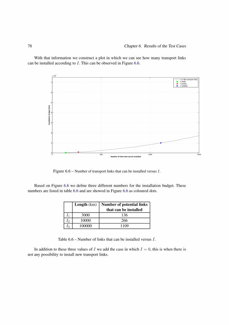
78 Chapter 6. Results of the Test Cases
With that information we construct a plot in which we can see how many transport linkscan be installed according to I . This can be observed in Figure 6.6.
0 500 1000 15000
1
2
3
4
5
6
7
x 105
Number of links that can be installed
Inst
alla
tio
n b
ud
get
(km
)
I vs Nbr transport linksI=3000I=10000I=100000
Figure 6.6 – Number of transport links that can be installed versus I .
Based on Figure 6.6 we define three different numbers for the installation budget. Thesenumbers are listed in table 6.6 and are showed in Figure 6.6 as coloured dots.
Length (km) Number of potential links
that can be installed
I1 3000 136I2 10000 266I3 100000 1109
Table 6.6 – Number of links that can be installed versus I .
In addition to these three values of I we add the case in which I = 0, this is when there isnot any possibility to install new transport links.
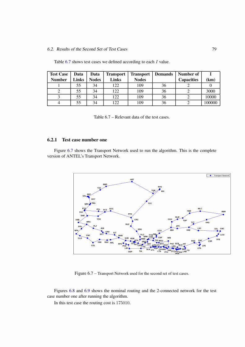
6.2. Results of the Second Set of Test Cases 79
Table 6.7 shows test cases we defined according to each I value.
Test Case Data Data Transport Transport Demands Number of I
Number Links Nodes Links Nodes Capacities (km)
1 55 34 122 109 36 2 02 55 34 122 109 36 2 30003 55 34 122 109 36 2 100004 55 34 122 109 36 2 100000
Table 6.7 – Relevant data of the test cases.
6.2.1 Test case number one
Figure 6.7 shows the Transport Network used to run the algorithm. This is the completeversion of ANTEL’s Transport Network.
SROSBT
SRM CHMFYM
CSP
RBL
CCO JBO
CCHOLM
TUP
FMRMLC
RBR
VRGTYT
VRELSC DJL CHC
LCO
STECSRCHF
LPELPA
ROC
HIT
FJIPPDLABRIAPA5
PEN
MLD
PTZ
LDS
PRPPYV
BSL
GAZ
CALLTN
LFS
PDPATLSLN
TIA
TIUATE
TAL MGU
MTC
MIN
PAZ SCR
ZPC
SAL
DAY
TRGQBC
PY3
PAY
SNR
FRBMRC
DOL
NPA
CLO
CNC
COL
TRR RSC NHL
MABSJM
RPZPVD
LIB
ODP
CAN
MND
FLC
SDG
DUZ
CRC
PTO
TCC
RVS
RIVTQR
ART
BBR
TAC
DEF
RDRVCA
CETSLC
ICTCRDSCT
JERPLT
GCCALG
YOU
PCL
Transport Network
Figure 6.7 – Transport Network used for the second set of test cases.
Figures 6.8 and 6.9 shows the nominal routing and the 2-connected network for the testcase number one after running the algorithm.
In this test case the routing cost is 175010.
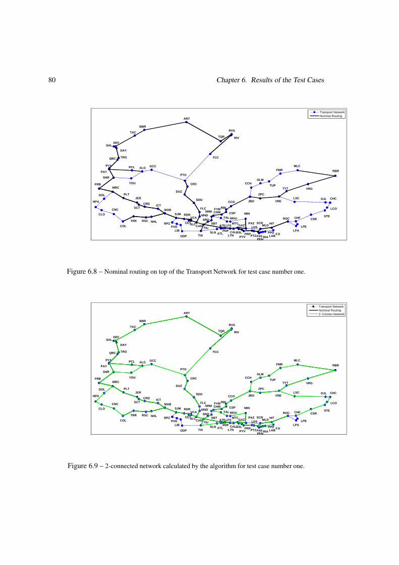
80 Chapter 6. Results of the Test Cases
SROSBT
SRM CHMFYM
CSP
RBL
CCO JBO
CCHOLM
TUP
FMRMLC
RBR
VRGTYT
VRELSC DJL CHC
LCO
STECSRCHF
LPELPA
ROC
HIT
FJIPPDLABRIAPA5
PEN
MLD
PTZ
LDS
PRPPYV
BSL
GAZ
CALLTN
LFS
PDPATLSLN
TIA
TIUATE
TAL MGU
MTC
MIN
PAZ SCR
ZPC
SAL
DAY
TRGQBC
PY3
PAY
SNR
FRBMRC
DOL
NPA
CLO
CNC
COL
TRR RSC NHL
MABSJM
RPZPVD
LIB
ODP
CAN
MND
FLC
SDG
DUZ
CRC
PTO
TCC
RVS
RIVTQR
ART
BBR
TAC
DEF
RDRVCA
CETSLC
ICTCRDSCT
JERPLT
GCCALG
YOU
PCL
Transport NetworkNominal Routing
Figure 6.8 – Nominal routing on top of the Transport Network for test case number one.
SROSBT
SRM CHMFYM
CSP
RBL
CCO JBO
CCHOLM
TUP
FMRMLC
RBR
VRGTYT
VRELSC DJL CHC
LCO
STECSRCHF
LPELPA
ROC
HIT
FJIPPDLABRIAPA5
PEN
MLD
PTZ
LDS
PRPPYV
BSL
GAZ
CALLTN
LFS
PDPATLSLN
TIA
TIUATE
TAL MGU
MTC
MIN
PAZ SCR
ZPC
SAL
DAY
TRGQBC
PY3
PAY
SNR
FRBMRC
DOL
NPA
CLO
CNC
COL
TRR RSC NHL
MABSJM
RPZPVD
LIB
ODP
CAN
MND
FLC
SDG
DUZ
CRC
PTO
TCC
RVS
RIVTQR
ART
BBR
TAC
DEF
RDRVCA
CETSLC
ICTCRDSCT
JERPLT
GCCALG
YOU
PCL
Transport NetworkNominal Routing2−Connex Network
Figure 6.9 – 2-connected network calculated by the algorithm for test case number one.
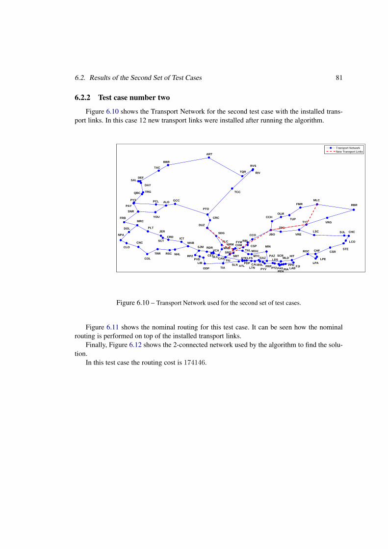
6.2. Results of the Second Set of Test Cases 81
6.2.2 Test case number two
Figure 6.10 shows the Transport Network for the second test case with the installed trans-port links. In this case 12 new transport links were installed after running the algorithm.
SROSBT
SRM CHMFYM
CSP
RBL
CCO JBO
CCHOLM
TUP
FMRMLC
RBR
VRGTYT
VRELSC DJL CHC
LCO
STECSRCHF
LPELPA
ROC
HIT
FJIPPDLABRIAPA5
PEN
MLD
PTZ
LDS
PRPPYV
BSL
GAZ
CALLTN
LFS
PDPATLSLN
TIA
TIUATE
TAL MGU
MTC
MIN
PAZ SCR
ZPC
SAL
DAY
TRGQBC
PY3
PAY
SNR
FRBMRC
DOL
NPA
CLO
CNC
COL
TRR RSC NHL
MABSJM
RPZPVD
LIB
ODP
CAN
MND
FLC
SDG
DUZ
CRC
PTO
TCC
RVS
RIVTQR
ART
BBR
TAC
DEF
RDRVCA
CETSLC
ICTCRDSCT
JERPLT
GCCALG
YOU
PCL
Transport NetworkNew Transport Links
Figure 6.10 – Transport Network used for the second set of test cases.
Figure 6.11 shows the nominal routing for this test case. It can be seen how the nominalrouting is performed on top of the installed transport links.
Finally, Figure 6.12 shows the 2-connected network used by the algorithm to find the solu-tion.
In this test case the routing cost is 174146.

82 Chapter 6. Results of the Test Cases
SROSBT
SRM CHMFYM
CSP
RBL
CCO JBO
CCHOLM
TUP
FMRMLC
RBR
VRGTYT
VRELSC DJL CHC
LCO
STECSRCHF
LPELPA
ROC
HIT
FJIPPDLABRIAPA5
PEN
MLD
PTZ
LDS
PRPPYV
BSL
GAZ
CALLTN
LFS
PDPATLSLN
TIA
TIUATE
TAL MGU
MTC
MIN
PAZ SCR
ZPC
SAL
DAY
TRGQBC
PY3
PAY
SNR
FRBMRC
DOL
NPA
CLO
CNC
COL
TRR RSC NHL
MABSJM
RPZPVD
LIB
ODP
CAN
MND
FLC
SDG
DUZ
CRC
PTO
TCC
RVS
RIVTQR
ART
BBR
TAC
DEF
RDRVCA
CETSLC
ICTCRDSCT
JERPLT
GCCALG
YOU
PCL
Transport NetworkNew Transport LinksNominal Routing
Figure 6.11 – Nominal routing on top of the Transport Network for test case number two.
SROSBT
SRM CHMFYM
CSP
RBL
CCO JBO
CCHOLM
TUP
FMRMLC
RBR
VRGTYT
VRELSC DJL CHC
LCO
STECSRCHF
LPELPA
ROC
HIT
FJIPPDLABRIAPA5
PEN
MLD
PTZ
LDS
PRPPYV
BSL
GAZ
CALLTN
LFS
PDPATLSLN
TIA
TIUATE
TAL MGU
MTC
MIN
PAZ SCR
ZPC
SAL
DAY
TRGQBC
PY3
PAY
SNR
FRBMRC
DOL
NPA
CLO
CNC
COL
TRR RSC NHL
MABSJM
RPZPVD
LIB
ODP
CAN
MND
FLC
SDG
DUZ
CRC
PTO
TCC
RVS
RIVTQR
ART
BBR
TAC
DEF
RDRVCA
CETSLC
ICTCRDSCT
JERPLT
GCCALG
YOU
PCL
Transport NetworkNew Transport LinksNominal Routing2−Connex Network
Figure 6.12 – 2-connected network calculated by the algorithm for test case number two.
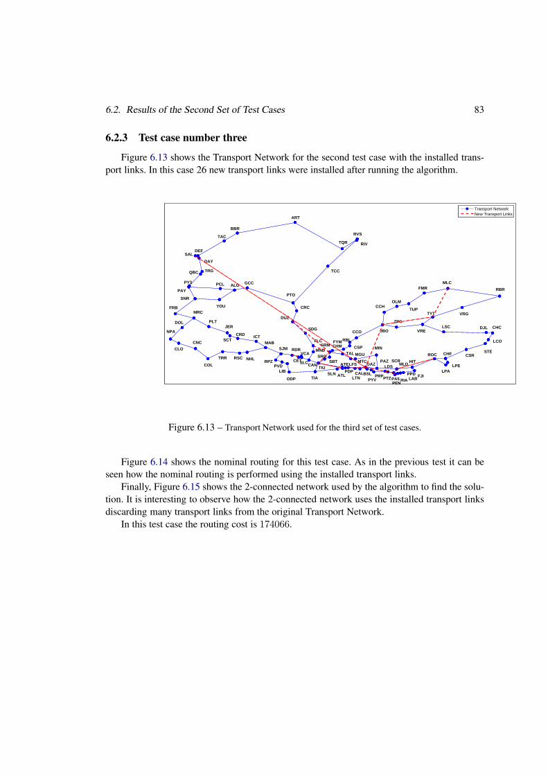
6.2. Results of the Second Set of Test Cases 83
6.2.3 Test case number three
Figure 6.13 shows the Transport Network for the second test case with the installed trans-port links. In this case 26 new transport links were installed after running the algorithm.
SROSBT
SRM CHMFYM
CSP
RBL
CCO JBO
CCHOLM
TUP
FMRMLC
RBR
VRGTYT
VRELSC DJL CHC
LCO
STECSRCHF
LPELPA
ROC
HIT
FJIPPDLABRIAPA5
PEN
MLD
PTZ
LDS
PRPPYV
BSL
GAZ
CALLTN
LFS
PDPATLSLN
TIA
TIUATE
TAL MGU
MTC
MIN
PAZ SCR
ZPC
SAL
DAY
TRGQBC
PY3
PAY
SNR
FRBMRC
DOL
NPA
CLO
CNC
COL
TRR RSC NHL
MABSJM
RPZPVD
LIB
ODP
CAN
MND
FLC
SDG
DUZ
CRC
PTO
TCC
RVS
RIVTQR
ART
BBR
TAC
DEF
RDRVCA
CETSLC
ICTCRDSCT
JERPLT
GCCALG
YOU
PCL
Transport NetworkNew Transport Links
Figure 6.13 – Transport Network used for the third set of test cases.
Figure 6.14 shows the nominal routing for this test case. As in the previous test it can beseen how the nominal routing is performed using the installed transport links.
Finally, Figure 6.15 shows the 2-connected network used by the algorithm to find the solu-tion. It is interesting to observe how the 2-connected network uses the installed transport linksdiscarding many transport links from the original Transport Network.
In this test case the routing cost is 174066.
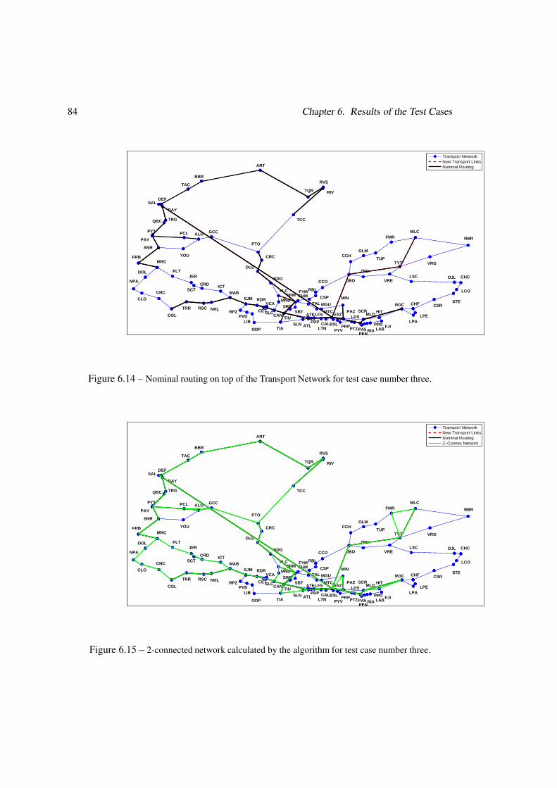
84 Chapter 6. Results of the Test Cases
SROSBT
SRM CHMFYM
CSP
RBL
CCO JBO
CCHOLM
TUP
FMRMLC
RBR
VRGTYT
VRELSC DJL CHC
LCO
STECSRCHF
LPELPA
ROC
HIT
FJIPPDLABRIAPA5
PEN
MLD
PTZ
LDS
PRPPYV
BSL
GAZ
CALLTN
LFS
PDPATLSLN
TIA
TIUATE
TAL MGU
MTC
MIN
PAZ SCR
ZPC
SAL
DAY
TRGQBC
PY3
PAY
SNR
FRBMRC
DOL
NPA
CLO
CNC
COL
TRR RSC NHL
MABSJM
RPZPVD
LIB
ODP
CAN
MND
FLC
SDG
DUZ
CRC
PTO
TCC
RVS
RIVTQR
ART
BBR
TAC
DEF
RDRVCA
CETSLC
ICTCRDSCT
JERPLT
GCCALG
YOU
PCL
Transport NetworkNew Transport LinksNominal Routing
Figure 6.14 – Nominal routing on top of the Transport Network for test case number three.
SROSBT
SRM CHMFYM
CSP
RBL
CCO JBO
CCHOLM
TUP
FMRMLC
RBR
VRGTYT
VRELSC DJL CHC
LCO
STECSRCHF
LPELPA
ROC
HIT
FJIPPDLABRIAPA5
PEN
MLD
PTZ
LDS
PRPPYV
BSL
GAZ
CALLTN
LFS
PDPATLSLN
TIA
TIUATE
TAL MGU
MTC
MIN
PAZ SCR
ZPC
SAL
DAY
TRGQBC
PY3
PAY
SNR
FRBMRC
DOL
NPA
CLO
CNC
COL
TRR RSC NHL
MABSJM
RPZPVD
LIB
ODP
CAN
MND
FLC
SDG
DUZ
CRC
PTO
TCC
RVS
RIVTQR
ART
BBR
TAC
DEF
RDRVCA
CETSLC
ICTCRDSCT
JERPLT
GCCALG
YOU
PCL
Transport NetworkNew Transport LinksNominal Routing2−Connex Network
Figure 6.15 – 2-connected network calculated by the algorithm for test case number three.

6.2. Results of the Second Set of Test Cases 85
6.2.4 Test case number four
Figure 6.16 shows the Transport Network for the second test case with the installed trans-port links. In this case 42 new transport links were installed after running the algorithm.
SROSBT
SRM CHMFYM
CSP
RBL
CCO JBO
CCHOLM
TUP
FMRMLC
RBR
VRGTYT
VRELSC DJL CHC
LCO
STECSRCHF
LPELPA
ROC
HIT
FJIPPDLABRIAPA5
PEN
MLD
PTZ
LDS
PRPPYV
BSL
GAZ
CALLTN
LFS
PDPATLSLN
TIA
TIUATE
TAL MGU
MTC
MIN
PAZ SCR
ZPC
SAL
DAY
TRGQBC
PY3
PAY
SNR
FRBMRC
DOL
NPA
CLO
CNC
COL
TRR RSC NHL
MABSJM
RPZPVD
LIB
ODP
CAN
MND
FLC
SDG
DUZ
CRC
PTO
TCC
RVS
RIVTQR
ART
BBR
TAC
DEF
RDRVCA
CETSLC
ICTCRDSCT
JERPLT
GCCALG
YOU
PCL
Transport NetworkNew Transport Links
Figure 6.16 – Transport Network used for the fourth set of test cases.
Figure 6.17 shows the nominal routing for this test case. It is interesting to observe that thenominal routing is performed using only installed links. This means that I was big enough toinstall direct links from and to all traffic endpoints. Thus, the routing cost find in this scenariois the minimum possible.
Finally, Figure 6.18 shows the 2-connected network used by the algorithm to find the solu-tion. This is the 2-connected network of minimum cost.
In this test case the routing cost is 159244.
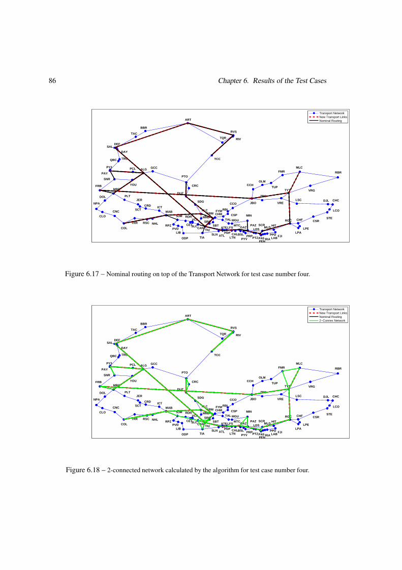
86 Chapter 6. Results of the Test Cases
SROSBT
SRM CHMFYM
CSP
RBL
CCO JBO
CCHOLM
TUP
FMRMLC
RBR
VRGTYT
VRELSC DJL CHC
LCO
STECSRCHF
LPELPA
ROC
HIT
FJIPPDLABRIAPA5
PEN
MLD
PTZ
LDS
PRPPYV
BSL
GAZ
CALLTN
LFS
PDPATLSLN
TIA
TIUATE
TAL MGU
MTC
MIN
PAZ SCR
ZPC
SAL
DAY
TRGQBC
PY3
PAY
SNR
FRBMRC
DOL
NPA
CLO
CNC
COL
TRR RSC NHL
MABSJM
RPZPVD
LIB
ODP
CAN
MND
FLC
SDG
DUZ
CRC
PTO
TCC
RVS
RIVTQR
ART
BBR
TAC
DEF
RDRVCA
CETSLC
ICTCRDSCT
JERPLT
GCCALG
YOU
PCL
Transport NetworkNew Transport LinksNominal Routing
Figure 6.17 – Nominal routing on top of the Transport Network for test case number four.
SROSBT
SRM CHMFYM
CSP
RBL
CCO JBO
CCHOLM
TUP
FMRMLC
RBR
VRGTYT
VRELSC DJL CHC
LCO
STECSRCHF
LPELPA
ROC
HIT
FJIPPDLABRIAPA5
PEN
MLD
PTZ
LDS
PRPPYV
BSL
GAZ
CALLTN
LFS
PDPATLSLN
TIA
TIUATE
TAL MGU
MTC
MIN
PAZ SCR
ZPC
SAL
DAY
TRGQBC
PY3
PAY
SNR
FRBMRC
DOL
NPA
CLO
CNC
COL
TRR RSC NHL
MABSJM
RPZPVD
LIB
ODP
CAN
MND
FLC
SDG
DUZ
CRC
PTO
TCC
RVS
RIVTQR
ART
BBR
TAC
DEF
RDRVCA
CETSLC
ICTCRDSCT
JERPLT
GCCALG
YOU
PCL
Transport NetworkNew Transport LinksNominal Routing2−Connex Network
Figure 6.18 – 2-connected network calculated by the algorithm for test case number four.
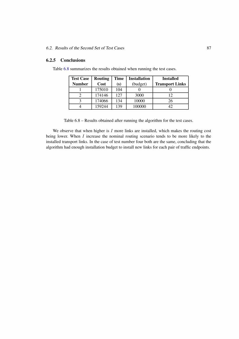
6.2. Results of the Second Set of Test Cases 87
6.2.5 Conclusions
Table 6.8 summarizes the results obtained when running the test cases.
Test Case Routing Time Installation Installed
Number Cost (s) (budget) Transport Links
1 175010 104 0 02 174146 127 3000 123 174066 134 10000 264 159244 139 100000 42
Table 6.8 – Results obtained after running the algorithm for the test cases.
We observe that when higher is I more links are installed, which makes the routing costbeing lower. When I increase the nominal routing scenario tends to be more likely to theinstalled transport links. In the case of test number four both are the same, concluding that thealgorithm had enough installation budget to install new links for each pair of traffic endpoints.

88 Chapter 6. Results of the Test Cases
Chapter 7
Conclusions
The present project addressed a complex and actual problem for many telecom operatorsthat is how to design and grow the capacity of their Transport Network in order to minimizethe routing cost of the data traffic generated in the Data Network.
First, we introduced the MOBCRN problem and presented the state of the art. After that,we showed that the MOBCRN problem is NP-Hard and designed a polynomial algorithm thatfinds solutions for the MOBCRN.
Following that point, we tested the algorithm against some other ways of solving similarproblems using the information from a real telecom operator, ANTEL. At this point we provedthat the algorithm performs as expected, giving similar values as the best ways of solving theproblem.
Finally, we tested the algorithm with the complete ANTEL’s network in a very complexscenario for different levels of installation budget, explaining the different outputs of the algo-rithm for each case.
Because of these points, we can conclude that the presented algorithm performes withinthe range of previous works, adding the possibility to evaluate the installation of new transportlinks. This not only allows a telecom operator to design its multi-overlay network, but also plana growth of its existing network. This was proved using real information showing good results,which is a clear example of the potential of this kind of tools.
89

90 Chapter 7. Conclusions

Chapter 8
Open Problems and Future Work
Despite the algorithm performs in the range of previous works in the same area, there aremany improvements that can be done in order to have faster and better solutions for the pro-blem.
On the one hand, the way the algorithm installs new links is far from being optimal. Thepresent algorithm installs links starting from the first traffic demand to be analyzed. This canfrequently produce situations in which the optimal set of installed links are not chosen. Apossible solution for this problem is to consider all possible combinations of installed linksaccording to the installation budget and keep the one that minimizes the routing cost. This wasdiscarded beacause that approach consumes a lot of computational resources. A more cleverway to solve it could be to formulate an integer programming model to assign the optimal setof installed links.
On the other hand, a similar situation is faced when we find the shortest paths for thenominal routing. As the algorithm runs a shortest-path algorithm for each flow separately, theoptimal solutions is not likely to be found.
As this algorithm only tries to minimize the routing cost for a given traffic scenario, it canbe intereseting to formulate a problem to study which is the combination of installed links thatproduces the minimun routing cost for a set of traffic scenarios that a telecom operator is likelyto experience during its day-by-day operation.
Moreover, it would also be intereseting to study wich is the set of links that minimizes theproduct between the installation budget and routing cost. This will help the operator to knownot only which transport links must be installed to optimize its network, but also how muchbudget they must consider.
A reformulation of the problem can also be performed to find solutions under unfeasiblescenarios as stated in Section 4.2.3. Covering these scenarios would help to find solutions to awider range of network configuations.
91
92 Chapter 8. Open Problems and Future Work
Bibliography
[1] 802.3 Ethernet Working Group. Technical report, Institute of Electrical and ElectronicsEngineers.
[2] EIBONE, Efficient Integrated Backbone project website.
[3] ITU-T Recommendation G.803: Architecture of transport networks based on the syn-chronous digital hierarchy (SDH). Technical report, International TelecommunicationUnion, 2004.
[4] ITU-T Recommendation X.200: Basic Reference Model: The basic model. Technicalreport, International Telecommunication Union, 2004.
[5] Fundamentals of DWDM Technology. Technical report, Cisco Networks, 2006.
[6] ITU-T Recommendation G.784: Management aspects of synchronous digital hierarchy(SDH) transport network elements. Technical report, International TelecommunicationUnion, 2006.
[7] ITU-T Recommendation G.783: Characteristics of synchronous digital hierarchy (SDH)equipment functional blocks. Technical report, International Telecommunication Union,2008.
[8] ITU-T Recommendation G.707: Network node interface for the synchronous digital hier-archy (SDH). Technical report, International Telecommunication Union, 2009.
[9] Dimitris Alevras, Martin Grötschel, and Roland Wessäly. A network dimensioningtool. In Preprint SC 96-49, Konrad-Zuse-Zentrum fur Informationstechnik, pages 49–96. Konrad-Zuse-Zentrum fur Informationstechnik, 1996.
[10] Yossi Azar and Oded Regev. Combinatorial algorithms for the unsplittable flow problem.Algorithmica, 2006.
[11] A. Balakrishnan, T. L. Magnanti, and P. Mirchandani. A dual-based algorithm for multi-level network design. Management Science, 40(5):567–81, 1994.
[12] Anantaram Balakrishnan, Thomas L. Magnanti, and Prakash Mirchandani. Modelingand heuristic worst-case performance analysis of the two-level network design problem.Management Science, 40(7):846–867, 1994.
93

94 Bibliography
[13] Anantaram Balakrishnan, Thomas L. Magnanti, and Prakash Mirchandani. Designinghierarchical survivable networks. Operations Research, 46(1):116–136, January 1998.
[14] Anantaram Balakrishnan, Thomas L. Magnanti, and Prakash Mirchandani. Connectivity-splitting models for survivable network design. Networks, 43(1):10–27, January 2004.
[15] R. Bhandari. Optimal physical diversity algorithms and survivable networks. Proc. 2nd
IEEE Symp. Computers and Communications (ISCC), pages 433–441, 1997.
[16] Daniel Bienstock, Sunil Chopra, Oktay Günlük, and Chih-Yang Tsai. Minimum costcapacity installation for multicommodity network flows. Mathematical Programming,81:177–199, 1998.
[17] Andrés Corez. Multi-overlay network planning by applying a variable neighbourhoodsearch approach. Master’s thesis, Universidad de la República Oriental del Uruguay,Montevideo, Uruguay, 2010.
[18] Francois Despaux. Optimización de una red de datos IP/MPLS sobre SDM/DWDM us-ando tabú search. Caso de estudio: Red de datos de un operador de telefonía nacional.Master’s thesis, Universidad de la República Oriental del Uruguay, Montevideo, Uruguay,2011.
[19] E. W. Dijkstra. In Numerische Mathematik, pages 269–271.
[20] Thomas A. Feo and Mauricio G.C. Resende. Greedy randomized adaptive search proce-dures. Journal of Global Optimization, 6:109–133, 1995.
[21] Bernard Fortz and Michael Poss. An improved benders decomposition applied to a multi-layer network design problem. Oper. Res. Lett., 37(5):359–364, 2009.
[22] Alexander Gersht and Alexander Shulman. A new algorithm for the solution of the min-imum cost multicommodity flow problem. 26th IEEE Conference In Decision and Con-
trol, 26:748–758, 1987.
[23] M. Grötschel, C.L. Monma, and M. Stoer. Design of survivable networks, 1993.
[24] D. Katz, Kompella K., and D. Yeung. RFC 3630: Traffic Engineering (TE) Extensions toOSPF Version 2. Technical report, IETF, 2003.
[25] Hervé Kerivin and A. Ridha Mahjoub. Design of survivable networks: A survey. In In
Networks, pages 1–21, 2005.
[26] Hervé Kerivin, Dritan Nace, and Thi-Tuyet-Loan Pham. Design of capacitated survivablenetworks with a single facility. IEEE/ACM Trans. Netw., 13(2):248–261, 2005.
[27] A.M.C.A. Koster, S. Orlowski, C. Raack, G. Baier, and T. Engel. Single-layer cuts formulti-layer network design problems. Telecommunications Modeling, Policy, and Tech-
nology, pages 1–23, 2008.
Bibliography 95
[28] T. L. Magnanti, P. Mirchandani, and R. Vachani. Modeling and Solving the Two-FacilityCapacitated Network Loading Problem. Operations Research, 43:142–157, 1995.
[29] T. Magnanti, P. Mirchandani, and R. Vachani. Modeling and solving the capacitated net-work loading problem. Operations Research Center Working Paper, 01:239–291, 1991.
[30] Haruko Okamura and P.D. Seymour. Multicommodity flows in planar graphs. Journal of
Combinatorial Theory, Series B, 31(1):75 – 81, 1981.
[31] P. Pan, Swallow G., and A. Atlas. RFC 4090: Fast Reroute Extensions to RSVP-TE forLSP Tunnels. Technical report, IETF, 2005.
[32] Cecilia Parodi. Integer Optimization Applied to the Design of Robust Minimum CostMulti-Layer Networks. Master’s thesis, Universidad de la República Oriental delUruguay, Montevideo, Uruguay, 2011.
[33] A. Bley, U. Menne, R. Klähne, C. Raack, and R. Wessäly. Multi-layer network design – Amodel-based optimization approach. In Proceedings of the 5th Polish-German Teletraffic
Symposium 2008, pages 107–116, Berlin, Germany, 2008.
[34] Christian Raack, Arie M.C.A. Koster, Sebastian Orlowski, and Roland Wessäly. On cut-based inequalities for capacitated network design polyhedra. Networks, 57(2):141–156,2011.
[35] S. Orlowski, A. Koster, C. Raack, and R. Wessäly. Two-layer network design by branch-and-cut featuring mip-based heuristics. In In Proceedings of the Third International Net-
work Optimization Conference. INOC, 2007.
[36] S. Ramamurthy and Biswanath Mukherjee. Survivable wdm mesh networks, part 1 -protection. In INFOCOM, pages 744–751, 1999.
[37] S. Ramamurthy and Biswanath Mukherjee. Survivable wdm mesh networks, part 2 -restoration. In INFOCOM, pages 2023–2030, 1999.
[38] Claudio Risso. Optimización de Costos en Redes Multicapa Robustas. Master’s thesis,Universidad de la República Oriental del Uruguay, Montevideo, Uruguay, 2010.
[39] E. Rosen, A. Viswanathan, and R. Callon. RFC 3031: Multiprotocol Label SwitchingArchitecture. Technical report, IETF, 2001.
[40] L. Sahasrabuddhe, S. Ramamurthy, and B. Mukherjee. Fault management in ip-over-wdmnetworks: Wdm protection versus ip restoration. IEEE J.Sel. A. Commun., 20(1):21–33,September 2006.
[41] K. Sunggy, G. Sahin, and S. Subramaniam. Cost efficient lsp protection in ip/mpls overwdm overlay networks. In In Communications, ICC 03. IEEE International Conference
on, pages 1278–1282 vol.2, 2003.
96 Bibliography
[42] M. Skutella. Approximating the single source unsplittable min-cost flow problem. In In
Foundations of Computer Science. Proceedings. 41st Annual Symposium on, pages 136–145, 2000.
[43] J. W. Suurballe and R. E. Tarjan. A quick method for finding shortest pairs of disjointpaths. Networks, 14(2):325–336, 1984.
[44] Robert Endre Tarjan. Deep-first search and linear graph algorithms. SIAM J. Comput.,1(2):146–160.
[45] Pushkar Tripathi. A deterministic algorithm for the vertex connectivity survivablenetwork design problem. Comput. Res. Repos. 2010, Article No. 1004.1208 (2010).
arXiv:1004.1208.
List of Figures
1.1 Example of multiple logical link failure from a single physical link failure. . . . . . . 101.2 Example of virtual links mapping into a Transport Network. . . . . . . . . . . . . . 111.3 Illustration of a Data Network implementing unsplitted (A) and splitted (B) data flows. 121.4 Examples of different technologies interacting in a stack structure. . . . . . . . . . . 121.5 Example of a multilayer network. . . . . . . . . . . . . . . . . . . . . . . . . . . 13
2.1 Example of a Data Network. . . . . . . . . . . . . . . . . . . . . . . . . . . . . 202.2 Example of a Transport Network. . . . . . . . . . . . . . . . . . . . . . . . . . . 222.3 Cost per transport technology. . . . . . . . . . . . . . . . . . . . . . . . . . . . . 232.4 Data Network example. . . . . . . . . . . . . . . . . . . . . . . . . . . . . . . . 252.5 Routes from v1 to v4 under ρD. . . . . . . . . . . . . . . . . . . . . . . . . . . . 262.6 Routing in the Transport Network. . . . . . . . . . . . . . . . . . . . . . . . . . . 27
4.1 Flow chart of the implementation of the MOBCRN. . . . . . . . . . . . . . . . . . 364.2 Transport Network with terminal nodes. . . . . . . . . . . . . . . . . . . . . . . . 374.3 Transport Network of the example . . . . . . . . . . . . . . . . . . . . . . . . . . 394.4 Transport Network of the Example. . . . . . . . . . . . . . . . . . . . . . . . . . 424.5 Connected subgraphs of the Example. . . . . . . . . . . . . . . . . . . . . . . . . 434.6 2-connected graphs of the Example. . . . . . . . . . . . . . . . . . . . . . . . . . 454.7 Transport routes in the 2-connected graph. . . . . . . . . . . . . . . . . . . . . . . 474.8 Transport routes in the 2-connected graph when link e = (t2, t9) fails. . . . . . . . . 484.9 Network of the example. . . . . . . . . . . . . . . . . . . . . . . . . . . . . . . 514.10 Data and Transport Network of the example. . . . . . . . . . . . . . . . . . . . . . 524.11 Transport Network of the example. . . . . . . . . . . . . . . . . . . . . . . . . . 574.12 Transport Network of the example - lines 1 to 2 of Pseudo-code 4.5:. . . . . . . . . . 584.13 Transport Network of the example. . . . . . . . . . . . . . . . . . . . . . . . . . 584.14 Transport Network of the example. . . . . . . . . . . . . . . . . . . . . . . . . . 584.15 Transport Network of the example. . . . . . . . . . . . . . . . . . . . . . . . . . 594.16 Transport Network of the example with the shortest path found by the SPA. . . . . . . 594.17 Unfeasible scenario. . . . . . . . . . . . . . . . . . . . . . . . . . . . . . . . . 60
5.1 ANTEL’s Transport Network. . . . . . . . . . . . . . . . . . . . . . . . . . . . . 645.2 East Region of ANTEL’s Transport Network. . . . . . . . . . . . . . . . . . . . . 655.3 West Region of ANTEL’s Transport Network. . . . . . . . . . . . . . . . . . . . . 65
97
98 List of Figures
5.4 Sub-network of the Transport Network of the example. . . . . . . . . . . . . . . . . 685.5 Sub-network of the Transport Network of the example with potential links. . . . . . . 68
6.1 Transport Network for the test case east_copy. . . . . . . . . . . . . . . . . . . 726.2 Nominal routing for the test case east_copy. . . . . . . . . . . . . . . . . . . . 736.3 2-connected network identified by the algorithm for the test case east_copy. . . . . 746.4 Distribution of the lengths of the potential transport links. . . . . . . . . . . . . . . 776.5 Cumulative distribution of the lengths of the potential transport links. . . . . . . . . . 776.6 Number of transport links that can be installed versus I . . . . . . . . . . . . . . . . 786.7 Transport Network used for the second set of test cases. . . . . . . . . . . . . . . . 796.8 Nominal routing on top of the Transport Network for test case number one. . . . . . . 806.9 2-connected network calculated by the algorithm for test case number one. . . . . . . 806.10 Transport Network used for the second set of test cases. . . . . . . . . . . . . . . . 816.11 Nominal routing on top of the Transport Network for test case number two. . . . . . . 826.12 2-connected network calculated by the algorithm for test case number two. . . . . . . 826.13 Transport Network used for the third set of test cases. . . . . . . . . . . . . . . . . 836.14 Nominal routing on top of the Transport Network for test case number three. . . . . . 846.15 2-connected network calculated by the algorithm for test case number three. . . . . . 846.16 Transport Network used for the fourth set of test cases. . . . . . . . . . . . . . . . . 856.17 Nominal routing on top of the Transport Network for test case number four. . . . . . . 866.18 2-connected network calculated by the algorithm for test case number four. . . . . . . 86


![Tesis - premat.fing.edu.uypremat.fing.edu.uy/ingenieriamatematica/archivos/... · enmarcados en Teoría de Grafos [12] y en la Sección2.2se realiza un breve resumen referente a la](https://img.dokumen.tips/doc/110x75/5f4b92b1a6486448cb69f7be/tesis-enmarcados-en-teora-de-grafos-12-y-en-la-seccin22se-realiza-un-breve.jpg)


