Agilent PNA Microwave Network Analyzers

Application Note 1408-12

Pulsed-RF S-Parameter Measurements Using Wideband and Narrowband Detection

2

Introduction . . . . . . . . . . . . . . . . . . . . . . . . . . . . . . . . . . . . . . . . . . . . . . . . . . . . . . . . . . . . . . . . . .3

Pulsed-RF measurement types . . . . . . . . . . . . . . . . . . . . . . . . . . . . . . . . . . . . . . . . . . . . . . . . .5

Average and point-in-pulse pulse measurements . . . . . . . . . . . . . . . . . . . . . . . . . . . . . . .6

Pulse profile measurements . . . . . . . . . . . . . . . . . . . . . . . . . . . . . . . . . . . . . . . . . . . . . . . . .7

Pulse-to-pulse measurements . . . . . . . . . . . . . . . . . . . . . . . . . . . . . . . . . . . . . . . . . . . . . . .8

Pulsed-RF Detection Techniques . . . . . . . . . . . . . . . . . . . . . . . . . . . . . . . . . . . . . . . . . . . . . . . .9

Overview of wideband detection . . . . . . . . . . . . . . . . . . . . . . . . . . . . . . . . . . . . . . . . . . . .10

Overview of narrowband detection . . . . . . . . . . . . . . . . . . . . . . . . . . . . . . . . . . . . . . . . . .11

Comparing the two techniques . . . . . . . . . . . . . . . . . . . . . . . . . . . . . . . . . . . . . . . . . . . . . .12

In-depth view of wideband detection . . . . . . . . . . . . . . . . . . . . . . . . . . . . . . . . . . . . . . . .13

In-depth view of narrowband detection . . . . . . . . . . . . . . . . . . . . . . . . . . . . . . . . . . . . . .20

Using spectral nulling for wider IF bandwidths . . . . . . . . . . . . . . . . . . . . . . . . . . . . . . . .24

Typical setup for forward pulsed-RF amplifier measurements . . . . . . . . . . . . . . . . . . .30

Pulling it all together with Option H08 . . . . . . . . . . . . . . . . . . . . . . . . . . . . . . . . . . . . . . .32

More Configuration Choices . . . . . . . . . . . . . . . . . . . . . . . . . . . . . . . . . . . . . . . . . . . . . . . . . .34

Hardware setups . . . . . . . . . . . . . . . . . . . . . . . . . . . . . . . . . . . . . . . . . . . . . . . . . . . . . . . . . .34

Reference signal choices . . . . . . . . . . . . . . . . . . . . . . . . . . . . . . . . . . . . . . . . . . . . . . . . . . .37

Pulse test sets . . . . . . . . . . . . . . . . . . . . . . . . . . . . . . . . . . . . . . . . . . . . . . . . . . . . . . . . . . . .38

Pulse generators . . . . . . . . . . . . . . . . . . . . . . . . . . . . . . . . . . . . . . . . . . . . . . . . . . . . . . . . . .39

IF gain setting . . . . . . . . . . . . . . . . . . . . . . . . . . . . . . . . . . . . . . . . . . . . . . . . . . . . . . . . . . . .40

Reference loop . . . . . . . . . . . . . . . . . . . . . . . . . . . . . . . . . . . . . . . . . . . . . . . . . . . . . . . . . . . .40

Measuring frequency converters . . . . . . . . . . . . . . . . . . . . . . . . . . . . . . . . . . . . . . . . . . . .40

Using power sweeps . . . . . . . . . . . . . . . . . . . . . . . . . . . . . . . . . . . . . . . . . . . . . . . . . . . . . .40

Calibration . . . . . . . . . . . . . . . . . . . . . . . . . . . . . . . . . . . . . . . . . . . . . . . . . . . . . . . . . . . . . . . . . .41

S-parameter measurements . . . . . . . . . . . . . . . . . . . . . . . . . . . . . . . . . . . . . . . . . . . . . . . .41

Source power calibration . . . . . . . . . . . . . . . . . . . . . . . . . . . . . . . . . . . . . . . . . . . . . . . . . . .41

Comparing the PNA and 8510 . . . . . . . . . . . . . . . . . . . . . . . . . . . . . . . . . . . . . . . . . . . . . . . . .43

Summary . . . . . . . . . . . . . . . . . . . . . . . . . . . . . . . . . . . . . . . . . . . . . . . . . . . . . . . . . . . . . . . . . . .47

Web Resources . . . . . . . . . . . . . . . . . . . . . . . . . . . . . . . . . . . . . . . . . . . . . . . . . . . . . . . . . . . . . .48

Table of Contents

3

Vector network analyzers are the primary tool for accurate characterization of RF andmicrowave components, providing precision measurements of both magnitude and phaseresponses. For many devices, a continuous-wave (CW) stimulus/response configurationis sufficient.

However, many RF and microwave amplifiers used in commercial and aerospace/defenseapplications require testing using a pulsed-RF stimulus. This application note focuses onnew pulsed-RF S-parameter measurement techniques and capability provided byAgilent’s PNA Series of microwave vector network analyzers. This application note discusses the advantages and disadvantages of the two detection techniques commonlyused (wideband and narrowband detection), and compares and contrasts the PNA seriesnetwork analyzers (including the PNA-L) with the former industry standard for pulsed S-parameter measurements, the 85108A pulsed RF-network analyzer system.

Figure 1 shows an example of a modern microwave system – in this case, a radar system.It is apparent from the block diagram that these systems are composed of many individualRF and microwave components, such as amplifiers, mixers, filters and antennas.Accurate magnitude and phase characterization of these components is critical for effective system simulation and verification. Some of these components can be testedwith conventional swept-CW signals; this will yield traditional S-parameter measure-ments. However, some of the components must be tested under pulsed-RF conditions tosimulate their intended operating environment. This application note covers the specificpulsed-RF measurements used most often and the techniques by which they areachieved.

Figure 1. Block diagram of a typical radar system

Introduction

AMPBPFCOHO

STALO

Receiverprotection

Pulsemodulator

PRFge nerator

PREDRIVERAMP

RFBPF

PULSEDPOWER

Tx

LNA

IFBPF

0o SPLITTE R

ADC

ADC

ANTENNA

TRANSMITTER / EXCITER

Digital signalprocessor

(range and Doppler FFT)

Radar dataprocessor

(tracking loops, etc.)

90 oCOHO

S/H

S/H

LIMITER

LPF

LPF

BB AMP

BB AMP

LPF

MMI

RECEIVER / SIGNAL PR OCESSOR

1stIFA

2nd LO

IFBPF

2nd

IFA

Frequencyagile LO

DUP LE XE R

4

Pulsed-RF component testing

The topic of pulsed-RF testing is often focused on measuring the pulses themselves. Thisis critical, for example, in evaluating radar system performance and effectiveness. Whenmeasuring components however, the pulses are merely the stimulus, and the vector network analyzer (VNA) measures the effect that the device under test (DUT) has on thepulsed stimulus. Any non-ideal behavior of the pulses themselves is removed from themeasurement since the VNA performs ratioed measurements. This means that each S-parameter measurement compares a measured reflection or transmission responsewith the incident signal, providing ratioed magnitude and phase results. Figure 2, showsthe configuration for measuring forward S-parameters: the R receiver measures the incident signal, the A receiver measures the reflection response, and the B receivermeasures the transmission response. S11 is the complex ratio of the A and R receivers,and S21 is the complex ratio of the B and R receivers.

Figure 2. Simplified vector network analyzer block diagram

Testing under pulsed-RF conditions is very valuable for devices that will be used in apulsed-RF environment, since the behavior of many components differs between CW andpulsed-stimulus test. For example, the bias of an amplifier might change during a pulse.Or, the amplifier might exhibit overshoot, ringing, or droop as a result of being stimulatedwith a pulse. Also, particularly for radar systems, measuring the transient behavior withinthe pulse is critical for understanding system operation. Unintended modulation on thepulse (UMOP) can cause system problems in radar systems such as decreased clutterrejection, decreased target velocity resolution, undesired spread of phased-array- antenna beam patterns, and unintentional identification of radar systems. Characterizingthe amplitude and phase versus time in the pulse is crucial to characterizing and containingUMOP.

Many devices simply cannot be tested with CW stimulus at the desired power levels. Forexample, many high-power amplifiers are not designed to handle the power dissipation ofcontinuous operation, and when testing on-wafer, many devices lack sufficient heat sinking for CW testing. Testing with pulses allows the test-power levels of these devicesto be consistent with actual operation, resulting in more realistic characterization withoutthermal-induced damage. Characterizing these devices on-wafer prevents devices whichdon’t meet their specifications from being packaged, saving the manufacturer considerabletime and money.

Receiver/detector

Reflected (A) Transmitted (B)Incident (R)

Signalseparation

Incident

Reflected

DUT

TransmittedSource

Processor/display

5

This section covers the four basic ways that pulsed-RF stimuli are used in conjunctionwith VNAs. The first two types are pulsed S-parameter measurements, where a singlecomplex data point is acquired for each carrier frequency. The data is displayed in the frequency domain as magnitude and/or phase of transmission and reflection (Figure 3).The third and fourth measurement types are done with a fixed-RF carrier, and display datain the time domain.

Figure 3. Average and point-in-pulse measurements

Pulsed-RF measurementtypes

trace point

Average pulse

Magnitude and phase data averaged over entire pulse width

Point-in-pulse

Magnitude and phase data averaged over specified acquisition width and position within pulse

VNA data display

Frequency domain

6

Average and point-in-pulse pulse measurements

Average pulse measurements make no attempt to position the trace point at a specificpoint within the pulse. For each carrier frequency, the displayed S-parameter representsthe average value of the pulse. This occurs for example when doing narrowband detec-tion without any receiver gating. Point-in-pulse measurements result from taking dataonly during a specified acquisition window within the pulse. This window must be specified in terms of time duration (width) and position within the pulse (delay). Thereare different ways to do this in hardware, depending on the type of detection used (Figure 4). With wideband detection, the window is generally set by the data samplingperiod (determined by the IF bandwidth of the instrument) and a specified delay. Withnarrowband detection the acquisition window is set with a hardware switch or “gate”,which only allows measurement of a slice of each pulse. The gating can be performed ineither the RF or IF portion of the measurement receiver (PNA Option H11 provides IFgates). Both wideband and narrowband point-in-pulse techniques will be covered indepth later on.

Figure 4. a) Narrowband detection uses hardware switches (gates) in the RF or IF path to definethe acquisition window. b) Broadband detection uses the sampling period to define the acquisitionwindow.

Data samples

Pulsed IF

Point-in-pulseacquisition window

Narrowband detection

Broadband detection

Anti-alias filter

ADCIF gate

Digital FIR IF filter

Pulsed IF

Anti-alias filter

ADCRF gate

Digital FIR IF filter

Pulsed RF

a) b)

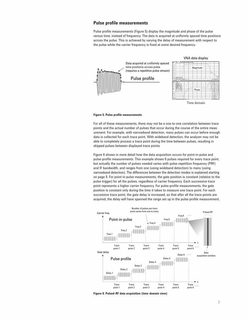
Pulse profile measurements

Pulse profile measurements (Figure 5) display the magnitude and phase of the pulse versus time, instead of frequency. The data is acquired at uniformly spaced time positionsacross the pulse. This is achieved by varying the delay of measurement with respect tothe pulse while the carrier frequency is fixed at some desired frequency.

Figure 5. Pulse profile measurements

For all of these measurements, there may not be a one-to-one correlation between tracepoints and the actual number of pulses that occur during the course of the entire meas-urement. For example, with narrowband detection, many pulses can occur before enoughdata is collected for each trace point. With wideband detection, the analyzer may not beable to completely process a trace point during the time between pulses, resulting inskipped pulses between displayed trace points.

Figure 6 shows in more detail how the data acquisition occurs for point-in-pulse andpulse-profile measurements. This example shows 6 pulses required for every trace point,but actually the number of pulses needed varies with pulse-repetition frequency (PRF)and IF bandwidth, and ranges from one (using wideband detection) to many (using narrowband detection). The differences between the detection modes is explained startingon page 9. For point-in-pulse measurements, the gate position is constant (relative to thepulse trigger) for all the pulses, regardless of carrier frequency. Each successive tracepoint represents a higher carrier frequency. For pulse-profile measurements, the gateposition is constant only during the time it takes to measure one trace point. For eachsuccessive trace point, the gate delay is increased, so that after all the trace points areacquired, the delay will have spanned the range set up in the pulse-profile measurement.

Figure 6. Pulsed-RF data acquisition (time-domain view)

7

VNA data display

Pulse profile

Data acquired at uniformly spaced time positions across pulse (requires a repetitive pulse stream)

dB

de g

Magnitude

Phase

Time domain

tTrace

point 1Trace

point 2Trace

point 3Trace

point 4Trace

point 5Trace

point 6. . .

Freq 1

Freq 2

Freq 3

Freq 4

Freq 5

Freq 6 . . .

Point-in-pulse

Pulse profile

Delay 1

Delay 2

Delay 3

Delay 4

Delay 5

Delay 6 . . . Data acquisition window

Number of pulses per trace point varies from one to many

Carrier freq Pulsed-RF

Gate delay

tTrace

point 1Trace

point 2Trace

point 3Trace

point 4Trace

point 5Trace

point 6. . .

8

Pulse-to-pulse measurements

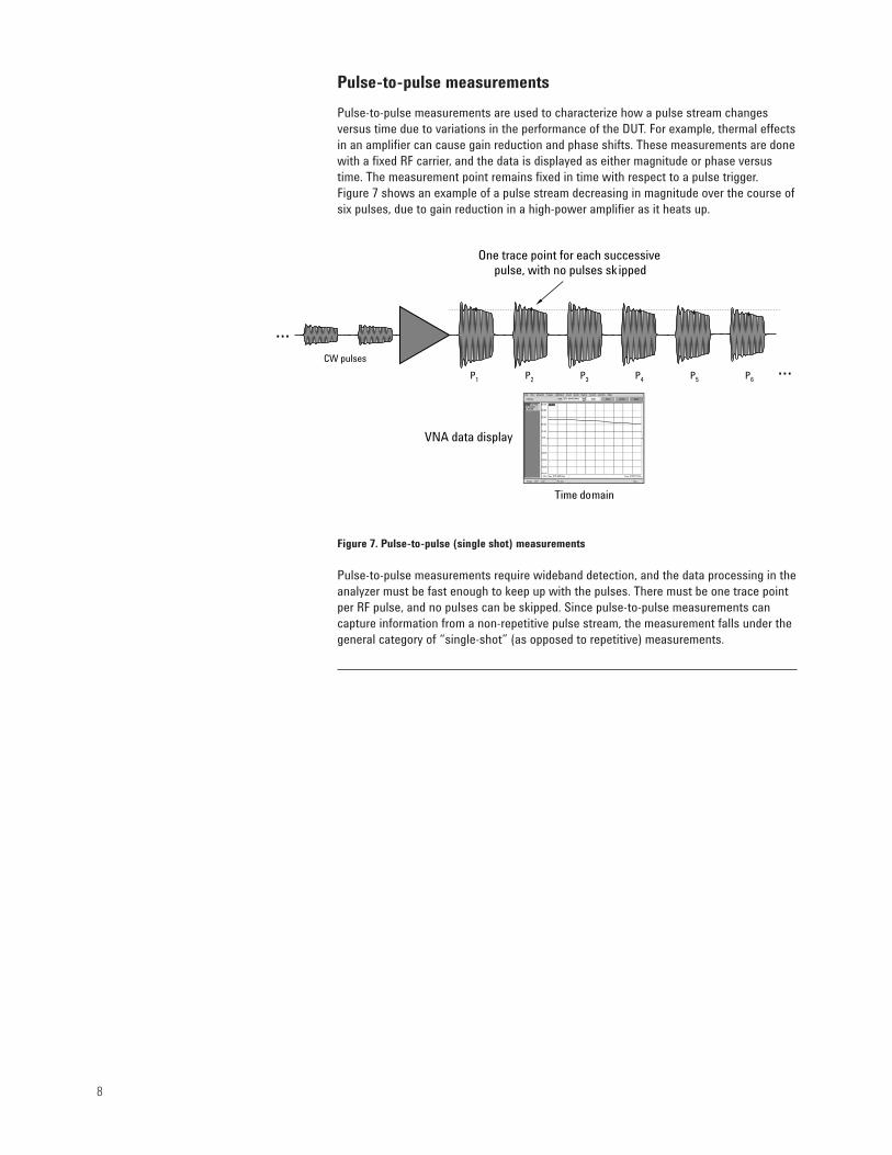
Pulse-to-pulse measurements are used to characterize how a pulse stream changes versus time due to variations in the performance of the DUT. For example, thermal effectsin an amplifier can cause gain reduction and phase shifts. These measurements are donewith a fixed RF carrier, and the data is displayed as either magnitude or phase versustime. The measurement point remains fixed in time with respect to a pulse trigger. Figure 7 shows an example of a pulse stream decreasing in magnitude over the course ofsix pulses, due to gain reduction in a high-power amplifier as it heats up.

Figure 7. Pulse-to-pulse (single shot) measurements

Pulse-to-pulse measurements require wideband detection, and the data processing in theanalyzer must be fast enough to keep up with the pulses. There must be one trace pointper RF pulse, and no pulses can be skipped. Since pulse-to-pulse measurements can capture information from a non-repetitive pulse stream, the measurement falls under thegeneral category of “single-shot” (as opposed to repetitive) measurements.

One trace point for each successive pulse, with no pulses sk ipped

P1 P2 P3 P4 P5 P6...

...CW pulses

VNA data display

Time domain

9

The next section provides an overview of the two different detection techniques, wideband and narrowband, commonly used in network analyzers. Each detection technique has its advantages and disadvantages. However, either technique can be usedto accurately measure S-parameters of amplifiers.

This application note assumes the reader is already familiar with pulsed-RF measure-ments. The basic concepts of pulsed RF are reviewed in Figure 8. When a signal isswitched on and off in the time domain (i.e., “pulsed”), the signal’s spectrum in the frequency domain has a sin(x)/x response. The widths of the lobes are inversely relatedto the pulse width (PW). This means that as the pulses get shorter in duration, the spectral energy is spread across a wider bandwidth. The spacing between the variousspectral components is equal to the pulse repetition frequency (PRF). If the PRF is 10 kHz, then the spacing of the spectral components is 10 kHz. In the time domain, therepetition of pulses is expressed as pulse repetition interval (PRI) or pulse repetition period (PRP), which are two terms for the same thing.

Figure 8. Pulsed-RF network-analysis terminology

Another important measure of a pulsed RF signal is its duty cycle. This is the amount oftime the pulse is on, compared to the period of the pulses. A duty cycle of 1.0 (100%)would be a CW signal. A duty cycle of 0.1 (10%) means that the pulse is on for one-tenthof the overall pulse period. For a fixed pulse width, increasing the PRF will increase theduty cycle. For a fixed PRF, increasing the pulse width increases the duty cycle. Dutycycle is an important pulse parameter for narrowband detection.

Measured S-parameterPulse width (PW)

1/PW

Duty cycle = on time /(on +off time)

= PW/PRI

f

Pulse repetition frequency(PRF = 1/PRI)

Time domain

Carrier frequency (fc)

Pulse repetition period (PRP)Pulse repetition interval (PRI)

Frequency domain

Pulsed-RF DetectionTechniques

10

Overview of wideband detection

Wideband detection can be used when the majority of the pulsed-RF spectrum is withinthe bandwidth of the receiver, as shown in Figure 9. In this case, the pulsed-RF signal willbe demodulated in the instrument, producing baseband pulses. This detection can beaccomplished with analog circuitry or with digital-signal processing (DSP) techniques.With wideband detection, the analyzer must be synchronized with the pulse stream, sothat data acquisition only occurs when the pulse is in the “on” state. This means that apulse trigger must be supplied to the analyzer that is the same frequency as the PRF, andthat has the correct delay relative to the pulse stream. For this reason, this technique isalso called synchronous acquisition mode. 8510-based systems had a built-in pulse generator to synchronize the data acquisition, while the PNA relies on external pulsegenerators.

Figure 9. Wideband (synchronous) detection

The advantages of the wideband mode are the fast measurement speed, simplicity of thetest setup, and that there is no loss in dynamic range when the pulses have a low dutycycle (i.e., a long time interval between pulses). Measurements take longer as duty cycledecreases, but since the analyzer is always sampling when the pulse is on, the signal-to-noise ratio is essentially constant versus duty cycle.

There are two disadvantages to using wideband detection. The first is that, compared tonarrowband detection, the noise floor of the instrument is higher due to the wider IFbandwidth used for detection. In the 8510, for example, this limited the best-case dynamicrange to approximately 60 dB. Another disadvantage of this technique is that there is alower limit to measurable pulse widths. As the pulse width gets smaller, the spectralenergy spreads out—once enough of the energy is outside the bandwidth of the receiver,the instrument cannot detect the pulses properly. Another way to think about it in thetime domain is that when the pulses are significantly shorter than the rise time of thereceiver, they cannot be detected. In the 8510, the narrowest pulse width that could beused was about 1 us.

Generally, if the pulse width required for testing the DUT is long enough to use widebanddetection, it is the preferred method.

Receiver BW

Pulse triggerFrequency domain

Time domain

11

Overview of narrowband detection

Narrowband detection is used when the bandwidth of the receiver is too small to containthe significant energy of the pulsed-RF spectrum. Since the pulsed-RF signal cannot befully captured, the analyzer goes to the other extreme: filter everything away except forone spectral component, as shown in Figure 10. With narrowband detection, all of the pulse spectrum is removed by analog or DSP-based filtering except for the central frequency component, which represents the frequency of the RF carrier. After filtering,the pulsed-RF signal appears as a sinusoidal (CW) signal, so there is no need to synchronizethe analyzer samples with the incoming pulses, and a pulse acquisition trigger is notrequired. Because an acquisition trigger is not used for narrowband detection, the technique is also called asynchronous acquisition mode.

Figure 10. Narrowband (asynchronous) detection

Although a data acquisition trigger is not needed for narrowband detection, it should benoted that, when gating is employed, the gate switches do require a synchronous triggerso that the gate is turned on during some portion of the time when the pulse is also on.However, since gating is not an essential element of narrowband detection, the techniqueis still considered as an asynchronous process.

When older network analyzers like the 8510 use narrowband detection, the PRF has to behigh compared to the IF bandwidth, to ensure that all of the undesired spectral compo-nents are filtered away. For this reason, the technique is also sometimes called the “highPRF” mode.

Agilent developed a unique “spectral-nulling” technique for the PNA which enables narrowband detection using wider IF bandwidths than normal. This novel techniqueyields faster measurements than those obtained by conventional narrowband filtering,and lets the user trade dynamic range for speed.

The main advantage to narrowband detection is that there is no lower pulse-width limit,since no matter how broad the pulse spectrum is, most of it is filtered away anyway,leaving only the central spectral component. For example, the PNA in narrowband modecan easily make S-parameter measurements with 100 ns pulses. Another advantage isthat for duty cycles in the 1% to 100% range, measurement dynamic range is usually significantly better than that obtained from wideband detection, due to the narrower IFbandwidth filters that are used.

The disadvantage to narrowband detection is that measurement dynamic range decreasesas duty cycle decreases. As the duty cycle of the pulses gets smaller (i.e., a longer timeinterval between pulses), the average power of the pulses gets smaller, resulting in lesssignal-to-noise ratio. In the frequency domain, you can see this effect by observing themagnitude of each spectral component decrease as duty cycle decreased, resulting in decreased measurement dynamic range. This phenomenon is often called “pulsedesensitization”. The degradation in dynamic range (in dB) can be expressed as 20*log(duty cycle).

Time domainDynamic range degradation

= 20*log[duty cycle]

IF filter

Frequency domainIF filter

12

Comparing the two techniques

Figure 11 shows the effect of duty cycle on pulsed dynamic range. The 8510, using broadband detection, has around 62 dB of dynamic range, independent of duty cycle.Using narrowband detection, the PNA’s dynamic range decreases with decreasing dutycycle. For every factor of 10 decrease in duty cycle, the dynamic range is reduced by 20dB. The cross-over point is approximately 0.1% — this means that for duty cycles of 0.1%or more, the PNA will have as much or more dynamic range than an 85108A system. Thisduty cycle range covers most radar, electronic warfare, and wireless communicationsmeasurement applications. The PNA’s inherent high dynamic range (compared to the8510) helps it overcome the limitations of narrowband detection. Also, the PNA has theadvantage of being able to measure components needing pulses narrower than 1 us,which is the 8510’s limit.

Figure 11. Duty-cycle effect on pulsed dynamic range

Note that the x-axis of this chart is the system duty cycle, which takes into account anygating that the PNA uses for point-in-pulse or pulse-profiling measurements. If the gateis such that only one-fifth of each incoming pulse is measured, then the overall dutycycle is effectively reduced by a factor of 5.

In summary, wideband detection offers dynamic range independent of duty cycle, butthere is a limit to how narrow the pulsed stimulus can be. Narrowband detection has nolower pulse-width limit, but measurement dynamic range is proportional to duty cycle.For the pulse widths and repetition frequencies used in many radar applications, the PNAusing narrowband detection offers faster measurement speeds and more dynamic rangethan the 8510 using wideband detection.

Wideband detection

Narrowband detection Dyn

amic

rang

e (d

B)

60

40

20

0

Widebanddetection

8510

Narrowband detection PNA

Narrowband detection 8510

CommsRadar

Isothermal

100

80

100 10.0 1.0 0.1 0.01

D u ty cycle ( % )

13

In-depth view of wideband detection

This section compares how the 8510 and PNA hardware and firmware implement wideband detection. Figure 12 shows a simplified block diagram of the IF portion of an85108 (8510-based) pulsed-RF system. The incoming 20 MHz pulsed-IF signal is mixedwith a 20 MHz local oscillator to produce baseband I/Q pulses (this technique is calledsynchronous detection). The detection bandwidth is about 1.5 MHz for the I and Q outputs, which is equivalent to a 3 MHz pre-detection bandwidth. This bandwidth yieldspulses that have about a 300 ns rise time (1/t). The pulse width must be greater thanseveral t’s in order for the detector to fully respond to the pulses. Due to the bandwidthof the analog detector, the specified minimum pulse width for the 85108 is 1 us, but inpractice, the pulse width can be pushed down to perhaps 500 ns or so.

Figure 12. Time-domain view of wideband detection in the 85108 pulsed-RF system

After the pulses are detected, a fast sample-and-hold circuit is used prior to the relativelyslow (by today's standards) analog-to-digital converter (ADC). Once the pulses are digitized,magnitude and phase is calculated. The actual sample point can be programmed with anyarbitrary delay with respect to the pulse trigger. The user specifies this delay value toaccomplish point-in-pulse measurements. Pulse profiling is achieved by stepping thesample delay from arbitrary start and stop values to cover the duration of the pulse.

risetime (1/ τ ) = 300 ns

I

Q

Pulsed I/Q

t

Pulsed signal Baseband pulsed I/Q A/D

converter

I

Q

Pulsed I/Q

t

Pulse trigger

Fast sample/hold

Pulse profile achieved by increasing delay

of sample point

Sample delay

0o

90o20 MHz

fall time = 300 ns

I(t)

Q(t)

20 MHz IF

Broadband, analog synchronous detector

(BW ≈ 1.5 MHz per side)

14

Figure 13 is a conceptual block diagram of how the PNA achieves wideband detection.Since all of the PNA’s IF processing (filtering and detection) is done with DSP, the incom-ing pulsed-IF signal is sampled directly. To get one filtered trace point using the 35 kHz IFbandwidth of the PNA, five data samples are required (more on this later), which requires30 us of acquisition time (6 us per sample). However, due to the IF settling time, thepulse must be present about 20 us prior to sampling. This yields a minimum pulse widthof about 50 us. To achieve this value, the “auto-IF-gain” mode of the PNA’s receiversmust be turned off, and the IF gain must be set manually. This should be done empirically– the higher the IF gain, the better the dynamic range of the measurement, but careshould be taken to ensure that the PNA’s receivers are not in compression.

Figure 13. Time-domain view of wideband detection in the PNA

Note that the trigger delay of the PNA (the time between the external pulse trigger andwhen the PNA actually takes data) is about 70 us. This means the PNA must be triggeredabout 50 us before the pulse modulator is triggered. This 50 us of “pre-trigger” plus the20 us IF settling time gives 70 us.

The PNA-L, a lower-cost version of the PNA, can also perform wideband pulse detection.The PNA-L has a wider maximum IF bandwidth than the PNA, allowing wideband detection to work with pulses as narrow as 10 us or 2 us, depending on the model (see Figure 14). The “auto-IF-gain” mode must also be turned off to improve the IF settlingtime. Note that, unlike the PNA, the PNA-L cannot use narrowband detection with spectral nulling. The next section discusses narrowband detection for the PNA in moredetail.

...

PNA IF filter = 35 kHzP NA sample rate = 6 us/sampleNumber of samples = 5

Pulsed IF

30 us

PNA samples

Externalpulse

trigger

70 us trigger delay

30 us

...

...

20 us settling time

30 us acquisition time

50 us pre-trigger

1 2 3 4 5 1 2 3 4 5

Using the PNA:20 us settling + 30 us acquisition = 50 us minimum pulse width (using 35 kHz IF bandwidth)

15

Figure 14. PNA and PNA-L minimum pulse widths for wideband detection

Figure 15 shows a longer pulse than that shown in Figure 13, illustrating how the PNAcan perform point-in-pulse and pulse-profile measurements using wideband detection.The user specifies the position in the pulse where data is acquired by setting the delay ofthe PNA point trigger relative to the RF modulation trigger. The width of the acquisitionwindow (which determines the resolution of the point-in-pulse or pulse-profile measure-ment) is determined by the PNA’s IF bandwidth. Using the 35 kHz (recommended) IFbandwidth on the PNA, the smallest resolution that can be achieved using widebanddetection is 30 us. As you will see in the next section, narrowband detection and IF gatescan provide much higher resolution (20 ns or better).

Figure 15. Point-in-pulse measurements in the PNA using wideband detection

No2 us600 kHzPNA-L models(2-port, 6, 13.5 GHz; 4-port, 20 GHz)

Yes10 us250 kHzPNA-L models(2-port, 20, 40, 50 GHz)

Yes50 us40 kHzPNA models(20, 40, 50, 67 GHz)

IF auto-gain modeavailable?*

Minimumpulse width

MaximumIF bandwidth

* Note: for pulsed-RF measurements, the IF auto-gain mode should be turned off (i.e., set IF gains manually)

20 us settling time

12345

Pulsed IF

PNA samples

tPoint-in-

pulse delay

Modulation trigger

PNA point trigger

16

Figure 16 shows a typical PNA setup for making wideband pulsed-RF measurements.This configuration can be used for pulse-to-pulse measurements or for point-in-pulsemeasurements, when the pulse width is sufficiently wide. In this example, the pulse generator sets the overall pulse timing. The PNA’s trigger must be set as follows:

Trigger Source = ExternalTrigger Scope = ChannelChannel Trigger State = Point Sweep

Under External Trigger:Input Source = TRIG IN BNCLevel = Positive or Negative Edge

Besides setting the auto-IF-gain to off, the PNA’s sweep should be set to step-sweepmode, and the frequency-offset mode should be turned on with an offset of zero Hz. Thisensures the PNA’s source will remain phase-locked in the presence of a pulsed-RF reference signal.

Figure 16. Typical PNA hardware setup for wideband detection

External pulse generator(e.g., 81110A/81111A)

Output 1

Ref In

Cplr Thru

DUT

Output 2

External RF modulator(e.g., Z5623A H81 2-20 GHz)

To TRIG IN (rear panel)

Src Out

17

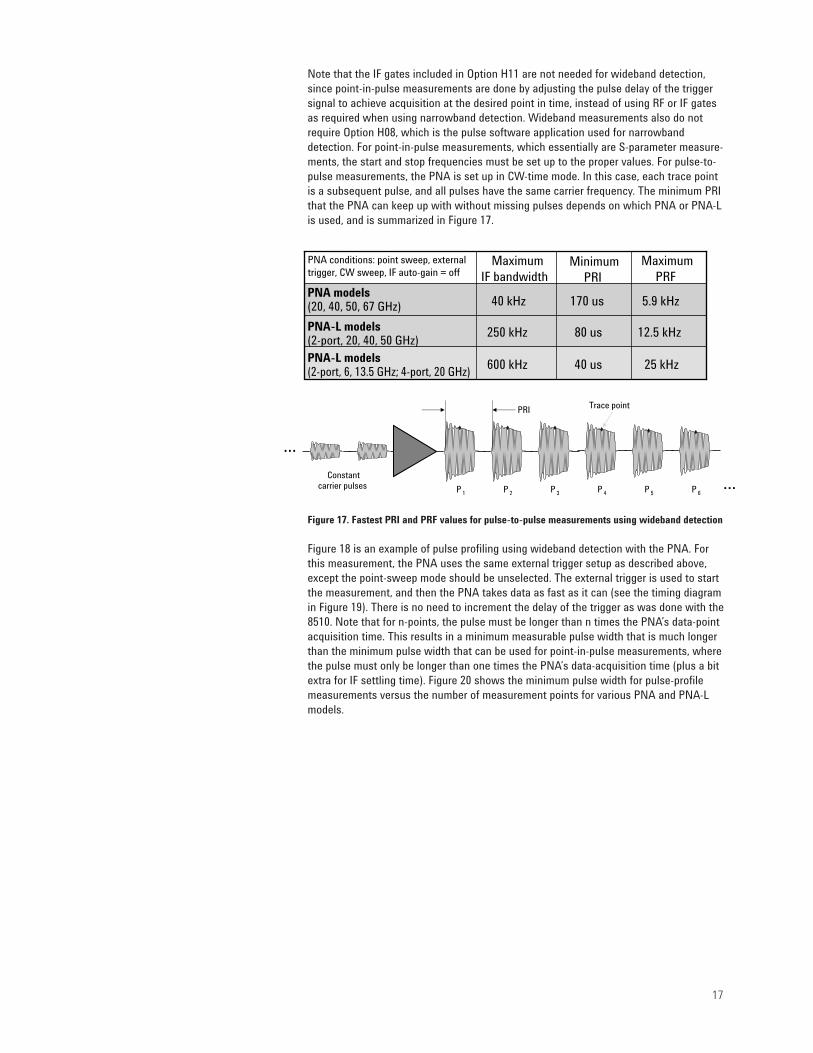
Note that the IF gates included in Option H11 are not needed for wideband detection,since point-in-pulse measurements are done by adjusting the pulse delay of the triggersignal to achieve acquisition at the desired point in time, instead of using RF or IF gatesas required when using narrowband detection. Wideband measurements also do notrequire Option H08, which is the pulse software application used for narrowband detection. For point-in-pulse measurements, which essentially are S-parameter measure-ments, the start and stop frequencies must be set up to the proper values. For pulse-to-pulse measurements, the PNA is set up in CW-time mode. In this case, each trace pointis a subsequent pulse, and all pulses have the same carrier frequency. The minimum PRIthat the PNA can keep up with without missing pulses depends on which PNA or PNA-Lis used, and is summarized in Figure 17.

Figure 17. Fastest PRI and PRF values for pulse-to-pulse measurements using wideband detection

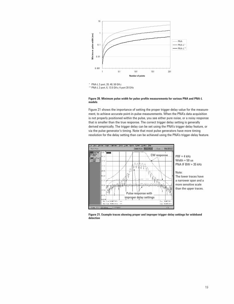
Figure 18 is an example of pulse profiling using wideband detection with the PNA. Forthis measurement, the PNA uses the same external trigger setup as described above,except the point-sweep mode should be unselected. The external trigger is used to startthe measurement, and then the PNA takes data as fast as it can (see the timing diagramin Figure 19). There is no need to increment the delay of the trigger as was done with the8510. Note that for n-points, the pulse must be longer than n times the PNA’s data-pointacquisition time. This results in a minimum measurable pulse width that is much longerthan the minimum pulse width that can be used for point-in-pulse measurements, wherethe pulse must only be longer than one times the PNA’s data-acquisition time (plus a bitextra for IF settling time). Figure 20 shows the minimum pulse width for pulse-profilemeasurements versus the number of measurement points for various PNA and PNA-Lmodels.

25 kHz40 us600 kHzPNA-L models(2-port, 6, 13.5 GHz; 4-port, 20 GHz)

12.5 kHz80 us250 kHzPNA-L models(2-port, 20, 40, 50 GHz)

5.9 kHz170 us40 kHzPNA models(20, 40, 50, 67 GHz)

MaximumPRF

MinimumPRI

MaximumIF bandwidth

PNA conditions: point sweep, externaltrigger, CW sweep, IF auto-gain = off

P 1 P 2 P 3 P 4 P 5 P 6

PRI Trace point

Constant carrier pulses ...

...

18

Figure 18. Pulse profile measurements in the PNA using wideband detection

Figure 19. Data acquisition for pulse profiling using the widest bandwidths of various PNA andPNA-L models

PW = 2 msPRF = 50 HzDuty cycle = 10%Points = 101IF BW = 35 kHz

PNA(40 kHz)

SampleTrace point

tAcquisition = 4 samples x 6 us/sample = 24 usTime per point = 24 us

PNA-L*(250 kHz)

tAcquisition = 4 samples x 1 us/sample = 4 usTime per point = 8 us

PNA-L**(600 kHz)

tAcquisition = 47 samples x 25 ns /sample = 1.175 usTime per point = 2.35 us

* 2-port, 20, 40, 50 GHz** 2-port, 6, 13.5 GHz; 4-port, 20 GHz

19

Figure 20. Minimum pulse width for pulse-profile measurements for various PNA and PNA-Lmodels

Figure 21 shows the importance of setting the proper trigger-delay value for the measure-ment, to achieve accurate point-in-pulse measurements. When the PNA’s data acquisitionis not properly positioned within the pulse, you see either pure noise, or a noisy responsethat is smaller than the true response. The correct trigger delay setting is generallyderived empirically. The trigger delay can be set using the PNA’s trigger-delay feature, orvia the pulse generator’s timing. Note that most pulse generators have more timing resolution for the delay setting than can be achieved using the PNA’s trigger-delay feature.

Figure 21. Example traces showing proper and improper trigger-delay settings for widebanddetection

0. 001

0. 01

0. 1

1

10

1 51 101 151 201

Min

imu

m p

ulse

wid

th (

ms)

PNA

PNA- L *

PNA- L **

* PNA-L 2-port, 20, 40, 50 GH z** PNA-L 2-port, 6, 13.5 GH z; 4-port 20 GHz

Number of points

PRF = 4 kHzWidth = 50 usPNA IF BW = 35 kHz

Note: The lower traces have a narrower span and a more sensitive scale than the upper traces.

CW response

Pulse response with improper delay settings

20

In-depth view of narrowband detection

This section focuses exclusively on the PNA and its unique “spectral nulling” techniquefor narrowband detection. Spectral nulling allows the use of wider bandwidths, improvingmeasurement speed (typically by a factor of 10 or more).

To understand how the spectral nulling works with narrowband detection, the pulsed-RFsignal with a 1.7 kHz PRF shown in Figure 22 will be used as an example. Figure 23shows a “zoomed-in” view around the central spectral component, which is shown in the“zero” or center position of the figure, since the pulsed-RF signal has been normalized tothe carrier frequency in this example. Due to the 1.7 kHz PRF, you expect to see spectralcomponents on either side of the carrier at intervals of 1.7 kHz. Only the first adjacentspectral components are shown in the figure. There are thousands of other spectral components present that are beyond the scale of the figure.

Figure 22. Pulsed-RF spectrum of narrowband measurement example

Figure 23. A zoomed-in view of the example pulse spectrum showing ideal and practical filterresponses

First null = 1/PW = 1/(7 us) = 143 kHz

PRF = 1.7 kHzPulse width = 7 usDuty cycle = 1.2%

First spectral sideband at 1.7 kHz ( = PRF)

Ideal filter

Desi red frequency component

Practical filters

3 dB bandwidth

Higher-selectivity (smaller shape factor) filter

21

If you could build an ideal filter to select the central spectral component but filter awayeverything else, it would look like a rectangle centered at zero Hz. A practical filter however requires a transition region between the passband and stopband. Typically, thestopband must be attenuated by 70 dB or more to filter out undesired spectral componentsand achieve sufficient measurement dynamic range. This means that the 3 dB bandwidthof the filter must be some fraction of the PRF. The value of the fraction depends on theselectivity of the filter. The selectivity is often expressed as shape factor, which is theratio of the 60 dB bandwidth divided by the 3 dB bandwidth. The smaller the shape factor,the faster the filter rolls off, and the wider the IF bandwidth that can be used for narrow-band detection. The figure shows that for a given 3 dB bandwidth, filters with differentshape factors will roll off at different rates.

Narrowband detection can be accomplished either with analog or digital filtering, asshown in Figure 24. To accommodate a wide range of PRFs, variable bandwidth filters arevery desirable to optimize measurement speed. The classic way to implement an analog,variable-bandwidth IF filter is by using the synchronously tuned topology. The heart of thefilter is a parallel LC (inductor/capacitor) resonator driven by a variable series resistance,usually achieved with a PIN diode. As the series resistance is increased, the bandwidthof the filter section gets smaller. Concatenating multiple resonator stages increases theselectivity of the filter.

Figure 24. Analog versus digital filtering

Variable-bandwidth digital filters are done using DSP algorithms performed after an analog-to-digital conversion occurs. There are two basic types of digital filters: finite-impulse response (FIR) and infinite-impulse response (IIR). The topologies of thesetwo filters differ, and each has their advantages and disadvantages. The bandwidth andselectivity (shape factor) of digital filters are controlled by the filter topology, number ofdelay elements, and weighting factors.

So, how wide a filter can the PNA use to successfully perform narrowband detection? Toanswer that question, you need to understand a little more how the PNA’s digital IF filterswork.

Classic analog variable-bandwidth bandpass filter:

Digital filtering: digital-signal processing afteranalog-to-digital conversion

Anti-alias filter

ADC Digital-signal processing

Z-1 Z-1x(n)

h(0) h(1) xx ...

+

22

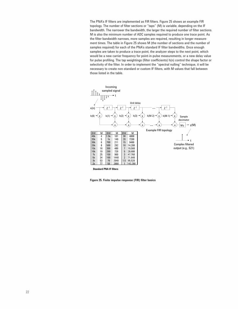
The PNA’s IF filters are implemented as FIR filters. Figure 25 shows an example FIR topology. The number of filter sections or “taps” (M) is variable, depending on the IFbandwidth. The narrower the bandwidth, the larger the required number of filter sections.M is also the minimum number of ADC samples required to produce one trace point. Asthe filter bandwidth narrows, more samples are required, resulting in longer measure-ment times. The table in Figure 25 shows M (the number of sections and the number ofsamples required) for each of the PNA’s standard IF filter bandwidths. Once enough samples are taken to produce a trace point, the analyzer steps to the next point, whichwould be a new carrier frequency for point-in-pulse measurements, or a new delay valuefor pulse profiling. The tap weightings (filter coefficients) h(n) control the shape factor orselectivity of the filter. In order to implement the “spectral nulling” technique, it will benecessary to create non-standard or custom IF filters, with M values that fall betweenthose listed in the table.

Figure 25. Finite impulse response (FIR) filter basics

Incoming sampled signal

t

Z-1 Z-1 Z-1 Z-1

x x

+

x

+

h(0) h(1) h(2) h(3)xx x

+...

h(M-2) h(M-1)

++

Unit delay

...x(n)

Sample decimator

y(M)M

Example FIR topology

Complex filtered output (e.g., S21)

t

MBWMBWMBW

1288050772k95,5201.5204070533k71,64021440100345k47,7603960150257k28,68057202001910k19,56074803001615k14,28010292500820k

948015211700630k7200201491k535k4800301011.5k440k

Standard PNA IF filters

143,280

23

Now that you know more about the digital filters in the PNA, you can look at their selectivity.Figure 26 shows two of the PNA’s standard filters in the frequency domain. It is clear thatthese are not ideal rectangular filters. The 100 Hz filter on the left requires ± 50 kHz toachieve stopband attenuation of 75 dB. Using the filter without any “tricks” (like spectralnulling) means the PRF must be 50 kHz or greater to ensure that the unwanted spectralcomponents are sufficiently filtered. In this case, the IF bandwidth would be 0.2% of thePRF. The shape factor of the 100 Hz filter is 400, compared to a typical spectrum-analyzerdigital-filter shape factor of about 4. For the 10 kHz filter, the PRF would have to begreater than 2.5 MHz to ensure that the unwanted spectral components are sufficientlyfiltered. In this case, the IF bandwidth would be 0.4% of the PRF. The shape factor of the10 kHz filter is 67, which is better than the 100 Hz filter, but is still far less selective thanthe filters on a spectrum analyzer. So, the standard IF filters, if used in a conventionalmanner, are not particularly well suited for narrowband pulse detection, as the IF band-widths must be very narrow compared to the PRF (typically between 1% and 0.1% of thePRF), resulting in slow measurements. VNA digital filters are not optimized for selectivity(as are spectrum analyzer filters), because for S-parameter measurements, the filter isalways exactly tuned to the incoming signal, or stated another way, the IF signal alwaysfalls in the center of the filter. With tracking filters, good selectivity is not needed.Instead, VNA filters are optimized for sweep speed and low noise bandwidth.

Figure 26. PNA IF filter shapes. a) 100 Hz filter with 100 kHz span. Shape factor = 400 b) 10 kHzfilter with 5 MHz span. Shape factor = 67

75 dB 75 dB

a) b)

24

Using spectral nulling for wider IF bandwidths

But wait! The story doesn’t end here. There are attributes of the digital IF filters in thePNA that allow you to improve our measurement speed significantly. Figure 27 shows atypical narrowband filter on the PNA (500 Hz in this case). If you look near the center ofthe filter response on the linear-magnitude trace, you will notice something very interest-ing. There appear to be nulls in the frequency response at periodic intervals. If you displaythe filter response with a log-magnitude format, the frequency nulls are quite clearlyseen. The frequency interval between nulls is directly proportional to the IF bandwidth,which in turn is inversely proportional to the number of sections of the digital filter, M.Note that the peaks of the filter response cause the poor selectivity seen in the previousfigure. Figure 28 shows how to take advantage of these nulls.

Figure 27. Close in view of the 500 Hz PNA IF filter

Figure 28. Filtered output using spectral nulling

log mag

lin mag

Frequency nulls exist at regular spacing (determined by M)

Apparent filter selectivity

Pulsed spectrum

X

Filtered outputDigital filter(with nulls aligned with PRF)

25

If the number of filter sections can be chosen such that the filter’s frequency nulls exactly align with the PRF, then the undesired pulsed spectral components will be filteredaway, leaving the desired center spectral component. PNA Option H08 allows these custom IF filters to be created. Instead of the standard 1, 1.5, 2, 3, 5, 7, 10 filter sequence,you can construct IF filters with arbitrary bandwidths like 421 Hz or 87 Hz. The bandwidthof these filters must be chosen based on the PRF, to ensure proper spectral nulling. Withthis technique, the IF bandwidth can be much higher compared to the conventional filtering shown previously, resulting in much faster measurement speed. In practice, if areally wide bandwidth is desired, the PRF of the pulses may need to be adjusted slightlyto ensure proper nulling. If the PRF cannot be adjusted, then the IF chosen will be as narrow as necessary to achieve proper spectral nulling.

Figure 29 shows the 500 Hz filter of Figure 27 superimposed on a 1.7 kHz PRF pulsestream. In this case the PNA is actually using every third null of the filter. This representsan IF bandwidth that is 29% of the PRF, instead of the 0.1 % to 1% required with conventional filtering.

Figure 29. Zoomed-in view of spectral nulling with 500 Hz filter (PRF = 1.7 kHz)

If you chose a narrower bandwidth to improve measurement dynamic range (at theexpense of measurement speed), the spectral components would skip more nulls. In thisway, you can trade off dynamic range and measurement speed by varying the IF bandwidth.

Response of 500 Hz digital IF filter and 1.7 kHz pulsed spectrum

-200

-180

-160

-140

-120

-100

-8 0

-6 0

-4 0

-2 0

0

Res

pons

e (d

B)

Frequency offset (Hz)

-500

0

-400

0

-300

0

-200

0

-100

0 0

100

0

200

0

300

0

400

0

500

0

Wanted frequency component

Filtered frequency components

26

Figure 30 shows what the nulling looks like when you narrow the IF filter bandwidth by afactor of 3, to 166 Hz. This example uses every ninth null of the filter, which representsan IF bandwidth that is about 9.9% of PRF, instead of the 0.1% to 1% required with conventional filtering. Narrowing the filter in this manner increases the dynamic range byabout 5 dB (10*log [3]).

Figure 30. Zoomed-in view of spectral nulling with 166 Hz filter (PRF = 1.7 kHz)

Figure 31 illustrates the speed differences between two traces that both use narrowbanddetection. One trace uses the PNA’s IF filters in a conventional manner, and the othertrace utilizes the spectral nulling technique. If the standard filter bandwidth is too large,then large amounts of trace noise can be seen, as shown in the two left-hand plots. Theright-hand plot shows that when both traces have approximately the same trace noise,spectral nulling results in a 14-fold improvement in measurement speed compared tousing conventional filtering.

Figure 31. IF bandwidth comparison, conventional filtering versus spectral-nulling

Response of 166 Hz digital IF filter and 1.7 kHz pulsed spectrum

-200

-180

-160

-140

-120

-100

-8 0

-6 0

-4 0

-2 0

0

Res

pons

e (d

B)

-500

0

-400

0

-300

0

-200

0

-100

0 0

100

0

200

0

300

0

400

0

500

0

Frequency offset (Hz) Wanted frequency component

Filtered frequency components

PRF = 2.349 kHzPW = 10 us (2.4% duty cycle)

With spectral nulling:IF BW = 415 Hz, sweep time = 1 sec

Without spectral nulling:IF BW = 30 Hz, sweep time = 14 sec

27

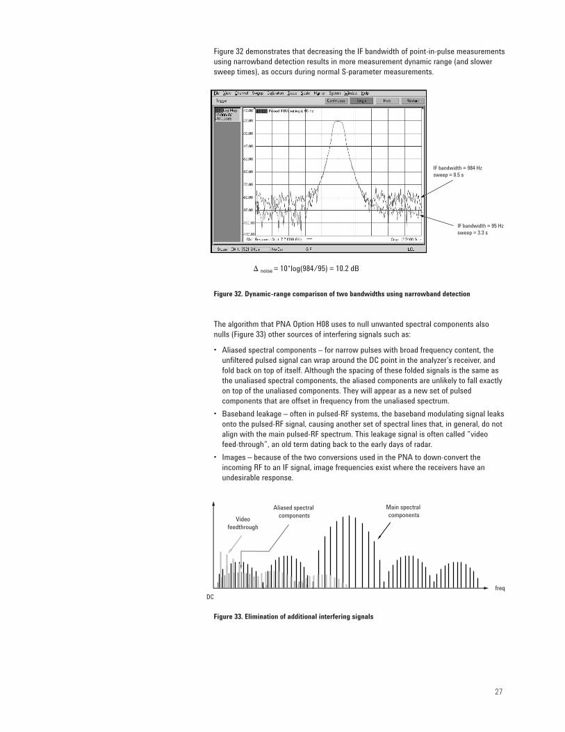
Figure 32 demonstrates that decreasing the IF bandwidth of point-in-pulse measurementsusing narrowband detection results in more measurement dynamic range (and slowersweep times), as occurs during normal S-parameter measurements.

Figure 32. Dynamic-range comparison of two bandwidths using narrowband detection

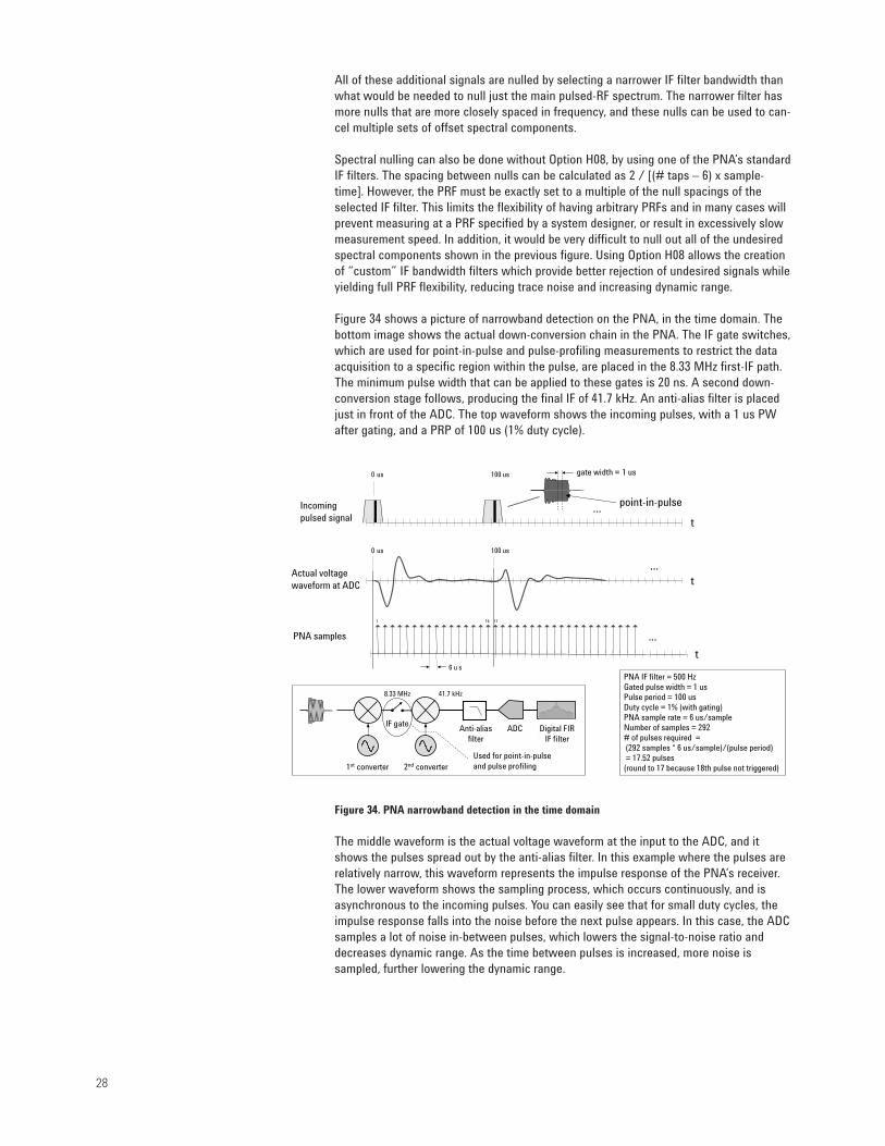
The algorithm that PNA Option H08 uses to null unwanted spectral components alsonulls (Figure 33) other sources of interfering signals such as:

• Aliased spectral components – for narrow pulses with broad frequency content, the unfiltered pulsed signal can wrap around the DC point in the analyzer’s receiver, and fold back on top of itself. Although the spacing of these folded signals is the same as the unaliased spectral components, the aliased components are unlikely to fall exactly on top of the unaliased components. They will appear as a new set of pulsed components that are offset in frequency from the unaliased spectrum.

• Baseband leakage – often in pulsed-RF systems, the baseband modulating signal leaksonto the pulsed-RF signal, causing another set of spectral lines that, in general, do not align with the main pulsed-RF spectrum. This leakage signal is often called “video feed-through”, an old term dating back to the early days of radar.

• Images – because of the two conversions used in the PNA to down-convert the incoming RF to an IF signal, image frequencies exist where the receivers have an undesirable response.

Figure 33. Elimination of additional interfering signals

IF bandwidth = 984 Hzsweep = 0.5 s

IF bandwidth = 95 Hzsweep = 3.3 s

D noise = 10*log(984/95) = 10.2 dB

Videofeedthrough

DCfreq

Aliased spectral components

Main spectral components

28

All of these additional signals are nulled by selecting a narrower IF filter bandwidth thanwhat would be needed to null just the main pulsed-RF spectrum. The narrower filter hasmore nulls that are more closely spaced in frequency, and these nulls can be used to can-cel multiple sets of offset spectral components.

Spectral nulling can also be done without Option H08, by using one of the PNA’s standardIF filters. The spacing between nulls can be calculated as 2 / [(# taps – 6) x sample-time]. However, the PRF must be exactly set to a multiple of the null spacings of theselected IF filter. This limits the flexibility of having arbitrary PRFs and in many cases willprevent measuring at a PRF specified by a system designer, or result in excessively slowmeasurement speed. In addition, it would be very difficult to null out all of the undesiredspectral components shown in the previous figure. Using Option H08 allows the creationof “custom” IF bandwidth filters which provide better rejection of undesired signals whileyielding full PRF flexibility, reducing trace noise and increasing dynamic range.

Figure 34 shows a picture of narrowband detection on the PNA, in the time domain. Thebottom image shows the actual down-conversion chain in the PNA. The IF gate switches,which are used for point-in-pulse and pulse-profiling measurements to restrict the dataacquisition to a specific region within the pulse, are placed in the 8.33 MHz first-IF path.The minimum pulse width that can be applied to these gates is 20 ns. A second down-conversion stage follows, producing the final IF of 41.7 kHz. An anti-alias filter is placedjust in front of the ADC. The top waveform shows the incoming pulses, with a 1 us PWafter gating, and a PRP of 100 us (1% duty cycle).

Figure 34. PNA narrowband detection in the time domain

The middle waveform is the actual voltage waveform at the input to the ADC, and itshows the pulses spread out by the anti-alias filter. In this example where the pulses arerelatively narrow, this waveform represents the impulse response of the PNA’s receiver.The lower waveform shows the sampling process, which occurs continuously, and isasynchronous to the incoming pulses. You can easily see that for small duty cycles, theimpulse response falls into the noise before the next pulse appears. In this case, the ADCsamples a lot of noise in-between pulses, which lowers the signal-to-noise ratio anddecreases dynamic range. As the time between pulses is increased, more noise is sampled, further lowering the dynamic range.

...

gate width = 1 us

point-in-pulse

0 us 100 us

Incoming pulsed signal t

0 us 100 us

...Actual voltage waveform at ADC t

1 16 17

PNA samples

1st converter 2nd converter

Anti-alias filter

ADCIF gate

Digital FIR IF filter

8.33 MHz 41.7 kHz

Used for point-in-pulse and pulse profiling

...t

6 u sPNA IF filter = 500 HzGated pulse width = 1 us Pulse period = 100 us Duty cycle = 1% (with gating)PNA sample rate = 6 us/sampleNumber of samples = 292# of pulses required = (292 samples * 6 us/sample)/(pulse period) = 17.52 pulses (round to 17 because 18th pulse not triggered)

29

Continuing with our example of a 500 Hz filter, 292 samples are required to produce oneS-parameter trace point. At 6 us per sample, this takes 1.75 ms. With our PRP of 100 us,we see that 17 pulses occur for each trace point that we acquire. Under normal conditions, the magnitude and phase of the pulses (at a given carrier frequency) are timeinvariant, so we get consistent and repeatable results. If the pulse response changes during the course of a measurement at a particular carrier frequency, then the resultingtrace point represents the average pulse response over the number of pulses used forthat trace point. The number of pulses required for a single trace point varies accordingto the PRF and the IF bandwidth. Because multiple pulses occur for each trace point, narrowband point-in-pulse measurements require a hardware gate before the ADC.

Figure 35 shows that decreased dynamic range with decreased duty cycle can easily beobserved on the network analyzer by measuring a device with high dynamic range, ahighpass filter in this example. Although filters are not normally measured under pulsedconditions, they do serve as useful DUTs to demonstrate pulse de-sensitization effects.

Figure 35. Duty-cycle versus dynamic range using narrowband detection and a high pass filter

In each plot, we compare a pulsed S-parameter (noisier trace) with a normal, swept-sinusoid S-parameter (cleaner trace). The top plot shows that with a 5% duty cycle, wecan still measure the filter stopband to about –60 dB with reasonable accuracy. The nextplot down (second from top), shows the effect of decreasing the duty cycle by a factor of three, resulting in a decrease in dynamic range of about 10 dB, and a rather noisymeasurement of the filter’s stopband. The next plot down (second from the bottom)shows that with another decrease in duty cycle (a factor of 10 this time), the analyzer’snoise floor has increased by 20 dB, and is now above the filter stopband all together.Note that the PW is 100 ns in this example. The lowest plot shows that we can improvedynamic range by averaging. 100 averages results in a 20 dB improvement in dynamicrange, so the measurement shows about the same dynamic range as the plot secondfrom the top. For all of these examples, a unique calibration was performed for each setof pulse conditions.

Pulse width = 100 nsDynamic range improved with averaging (101 avgs)

Pulse width = 3 µs (DC = 5.1%)

Pulse width = 1 µs (DC = 1.7%)

Pulse width = 100 ns (DC = 0.17%)

30

Typical setup for forward pulsed-RF amplifier measurements

Figure 36 shows a typical PNA setup for making narrowband pulsed-RF measurements inthe forward direction only, which often is all that is required for amplifier test. The exampleexternal test set is not just an RF modulator. It also includes an amplifier to boost thepower of test port 1. Higher test-port power is often needed for radar components liketransmit/receive (T/R) modules. The directional coupler is used to provide a referencesignal after the booster amplifier, so any drift of the booster amp is removed from themeasurement by ratioing. The test set is connected to the PNA via the front-panel RFjumpers provided by Option 014. For other applications, a simpler test set consisting solely of one or two RF modulators (switches) could also be used.

Figure 36. Typical PNA hardware setup for narrowband detection

The pulse generators, each with two output modules, provide the pulse timing to controlthe modulator and the PNA’s internal receiver gates, which are used for point-in-pulseand pulse-profile measurements. Typically, four pulse outputs are used: one each for theRF modulator, A-receiver gate and B-receiver gate, plus one for the two reference-receivergates, which can be tied together using a BNC tee. More complicated systems mightrequire more pulse output modules. The pulse generators are controlled via GPIB, andthe master pulse generator must be locked to the PNA’s 10 MHz timebase. The second(slave) pulse generator is synchronized via a front-panel trigger signal. The overall system (PNA and pulse generators) is controlled by the PNA Pulsed Application software(Option H08).

Option H08 VB application and DLL

Three output channels drive internal receiver gates A, B, and R1/R2 for point-in-pulse and pulse-profile measurements

Ref In

DUT

PNA

Trigger

GPIB

10 MHz Ref

Src Out

One output channel drives RF modulator

81110A family pulse generators

Z5623A H81 pulsed-RF test set

31

Figure 37 shows all of the PNA hardware options associated with a typical narrowbandpulsed-RF setup:

• 014 – Configurable test set• UNL – Source attenuators• 080 – Frequency-offset mode• 081 – Reference switch• H11 – IF access• 016 – Receiver attenuators (optional)

Figure 37. Typical PNA hardware options for narrowband detection

Option H11 adds the IF gating switches necessary for point-in-pulse and pulse-profilemeasurements. For a PNA configured with Option H11, Option 016 is the only “optional”option – all of the other options are required. Note that although the PNA uses dual-conversion receivers, only one conversion is shown for simplicity. Option H11 also addsexternal IF inputs and auxiliary RF and LO outputs. This additional hardware is necessaryfor antenna and mm-wave applications.

The IF gates supplied with Option H11 can only be used with Option H08. Option H08 alsoincludes the proprietary algorithms that implement the spectral nulling technique usedwith narrowband detection. In addition, Option H08 controls the pulse generator(s) used inthe system, and performs pulse-profile measurements.

Aux RF out (2-20 GHz)

Aux LO out (2-20 GHz)

Test port 1

Vtune

YIG source

Multipliers (1, 2, 4)

8.33 MHzreference

Phase-locked loop

Offset LO

Offset receiver

Option 080

Option 081

Test port 2

Option 014

Option UNL

Option 016

A

External IF in

ADC

IF gate

ADC

R2

External IF in

B

External IF in

ADC

IF gate

IF gate

Multipliers (1, 2)

Front

Rear Option H11

LOX

X

ADC

R1

External IF in

IF gateOption H11* Option H11*

Option H11* Option H11*

Option UNL

f*Option H11 notes:• IF-gate controls and external IF inputs are accessed on rear panel• IF gates are enabled with Option H08• External IF input frequency is 8.33 MHz

32

Pulling it all together with Option H08

Option H08 comes with two software components. One is a dynamic-link library (DLL)which acts as a “sub-routine”, and is needed for manual and automated environments.The second portion is a Visual Basic (VB) application that runs on the PNA. This VBapplication is used for stand-alone, bench-top use. It interacts with the DLL and sendsappropriate commands to the PNA and the pulse generator(s). The VB application isassigned to one of the PNA’s macro keys for easy access.

Figure 38 shows how Option H08 operates in the “software domain”. In stand-aloneoperation (indicated by the solid arrows), the VB application interacts with the DLL to getthe necessary spectral-nulling parameters. The VB application then sends these valuesto the PNA. The application also controls the pulse generators. The VB application doesnot have an application-programming interface (API), so in a remote environment wherethe user has their own software to control the pulse measurements, the user softwarecannot interact directly with the VB application. Instead, the user’s software must callthe DLL, and the returned values must then be sent to the PNA. The software must alsodirectly program the pulse generators. Remote operation is indicated by the dashedarrows.

Figure 38. Option H08 in the “software domain”

User softwarePNA + pulse generators

Option H08 VB syntax:Pulsed. ConfigNarrowBand(PRF, NumTaps, BW, OffSet, SampleRate, Precision)

Dynamic Link Library (.dll)(contains algorithms for spectral nulling)

Agilent pulse application (manual use only – no API available)

33

While the H08 application supports manual pulse profiling with the ability to save data, itdoes not support remote (software-controlled) pulse profiling. This can easily be accom-plished however with a small amount of program code (Figure 39). Basically, the delay ofthe pulse generator output(s) that controls the IF gate(s) for the signal or parameter youwish to profile is/are stepped in delay across a predetermined start and stop delay. Ateach delay, the PNA is triggered via software to make a single receiver or ratioed receiver(S-parameter) measurement. This is done in a loop. Agilent includes a Visual Basic programming example in the H08 documentation to demonstrate automated pulse-profilemeasurements.

Figure 39. Pulse profiling with user software

Most narrowband pulse applications for the PNA will require a combination of Option H11and Option H08. For cost-sensitive applications, a PNA without either option can be used,with limited flexibility and perhaps increased trace noise and degraded dynamic rangedue to sub-optimal spectral nulling. Option H08 can be used without H11 if average pulsemeasurements are sufficient (i.e., no point-in-pulse measurements), or if external RFswitches are used in place of the internal IF switches for point-in-pulse and pulse-profilemeasurements.

...

• S et carrier to a CW signal

• Increment delay of pulse generator(s) in a loop, for appropriate receiver(s)

• T rigger PNA (via software) to measure S-parameters at each delay setting

• After loops completes, read final trace data

Excerpt from VB programming example:For i = 0 To LNumPoints

OGPIB.ibwrt IPg, ":SOUR:PULS:DEL" & CStr(IOutput) & " " & CStr(H2oEdit_start.Value + H2oEdit_step.Value * i) & Chr$(10)

OGPIB.ibwrt IPg, "*OPC?" & Chr$(10)OGPIB.ibrd IPg, SOPCOApp.ManualTrigger Truepgb_meas.Value = i

Next

NoteOption H08 uses the frequency-offset option(Option 080) to ensure the PNA remains phase-locked with a pulsed reference signal. However,the frequency-offset value is not always zero Hz— sometimes, the application uses a frequencyoffset of 1.389 kHz to compensate for an internal data-acquisition sampling-frequencyshift. When this occurs and you try to set thePNA to its maximum stop frequency, an errorwill occur that says “Response frequenciesexceed instrument range”. To prevent this fromoccurring, set the stop frequency to a value thatis at least 2 kHz less than the maximumallowed. For example, on a 20 GHz PNA, set thestop frequency to 19.999998 GHz or less.

34

Hardware setups

Up to now, this application note has focused on two typical hardware setups, one eachfor wideband and narrowband detection. However, the PNA and PNA-L can be configuredin other ways for other pulsed-RF applications. The following examples illustrate the flexibility of the PNA and PNA-L platforms. Note that some signal lines have been omit-ted for clarity, such as 10 MHz references, pulse-generator-to-pulse-generator triggers,and GPIB connections. Also, more pulse generators than shown can be utilized forincreased flexibility of triggering the IF or RF gates when using narrowband detection.

Figure 40 shows an external RF switch used for receiver gating, instead of using thePNA’s internal IF gate switches. This setup, only used with narrowband detection, canprovide shorter gate widths (< 20 ns) than those obtained using the internal IF gates.This results in better timing resolution and lets you use a PNA without Option H11. Forforward, ratioed, pulse-profile measurements with coupled gates, a second RF switchwould be needed for the R1 reference channel.

Figure 40. Using an external RF switch for receiver gating (for narrowband detection)

More ConfigurationChoices

Ref In

+V -VCom

Power supplyTTL

DC(+)

Pulse2 out

External switch in receiver B loop for external gating

Pulse1 out

Src Out

DC(-)

DC supply used only if required by RF switch

35

Figure 41 shows a setup for forward and reverse (bi-directional) pulsed-RF S-parametermeasurements. This requires two RF switches for the modulators, and may or may notrequire the booster amplifiers and directional couplers shown in the figure. This configuration can be used with either wideband or narrowband detection. Note thatwhen using narrowband detection with this setup, the forward and reverse modulatorsand the R1 and R2 reference receiver gates share two pulse drives. If independent controlof the RF modulators and R1 and R2 receiver is desired for full flexibility, then six pulseoutput modules are needed, requiring a third pulse generator.

Figure 41. Forward and reverse (bi-directional) pulsed-RF S-parameter configuration

Figure 42 shows the PNA used with a pulsed RF signal created by pulsing the DC bias ofthe DUT. In this example, the input to the DUT is a swept CW signal, but the output is aswept pulsed-RF signal. The user has to supply the switches in the DC path of the amplifier, or use a power supply that can be pulsed on and off. This configuration can beused with wideband or narrowband detection. The setup is often used with widebanddetection to test output amplifiers of GSM mobile handsets.

Figure 42. Pulsed-bias S-parameter configuration

Narrowband detection:Three output channels drive internal receiver gates A, B, and R1/R2 for point-in-pulse and pulse-profile measurements

Wideband detection:One output channel drives PNA TRIG IN

Pulse1 out drives forward and reverse RF modulators

•

•

Power supply

Pulsed-RF

• Narrowband detection:Three output channels drive internal receiver gates A, B, and R1/R2 for point-in-pulse and pulse-profile measurements

• Wideband detection:One output channel drives PNA TRIG IN

Pulsed-DC bias to DUT

Pulse1 out

CWCom

+V -V

36

Figure 43 shows the combination of a pulsed-RF stimulus with pulsed-bias. This is a common configuration for on-wafer device test. Although this configuration can be usedfor on-wafer measurements with wideband or narrowband detection, very narrow pulsewidths are typically used, requiring narrowband detection. Note that when using narrow-band detection with this example, three pulse drives are used for the A, B and combinedR1/R2 IF gates. If independent control of all of the receiver gates is desired for full flexibility, then six pulse output modules are needed, requiring a third pulse generator.

Figure 43. Pulsed-RF and pulsed-bias S-parameter configuration

Power supply

DC(-)

Pulsed-DC bias to DUT

DC supply used here only if required by RF switch

Com+V -V

Narrowband detection:Three output channels drive internal receiver gates A, B, and R1/R2 for point-in-pulse and pulse-profile measurements

Wideband detection:One output channel drives PNA TRIG IN

•

•

Cplr thru

Src out

RF out

RF in

Pulse 2 out

TTL

DC(+)

Pulse 1 out

37

Reference signal choices

There are four ways in which the reference receiver can be used for pulsed S-parametermeasurements (Figure 44). A non-gated, CW stimulus (Figure 44a) gives the best dynamicrange as no pulse desensitization occurs in the reference channel, but the effect of thepulsed stimulus is not ratioed out of measurements of the DUT. For example, if the pulseduty cycle changes, the uncorrected S-parameter will change, since the test receiverexperiences a change in amplitude due to pulse desensitization, but the reference receiverdoes not. For most pulsed-RF S-parameter measurements, a pulsed signal for the referencereceiver is recommended (Figure 44b, 44d). Furthermore, gating all four receivers of thePNA is recommended (Figure 44d), as this allows use of unknown-through calibrations(i.e., short-open-load-reciprocal thru, or SOLR).

Pulse-profile measurements show the time-domain response of the pulse. For thesemeasurements, the reference receiver needs the pulsed stimulus so that the resultingprofile truly measures the effect of the DUT on the pulse’s magnitude and phase, withoutthe pulse’s inherent response affecting the results. Gating of the reference receivers isgenerally required for pulse-profile measurements (Figure 44d).

The configuration shown in Figure 44c is often used for a pulsed-DC-bias system withCW input.

Figure 44. Reference signal choices

Not gated

Gated

CW stimulus Pulsed stimulus

RF

Gate Gate

RF

a b

c d

38

Pulse test sets

Agilent can supply a variety of test sets for pulsed S-parameter measurements. Test sets include a single pulse modulator at a minimum, but may also include additional modulators, booster amplifiers, directional couplers, switches, and so on. The Z5623AH81 2-20 GHz RF modulator gives the PNA pulsed-RF system similar capability to the85108 in terms of frequency range and output power levels. With only one modulator,pulsed S-parameters can be done in the forward direction only, which is typical for amplifier measurements. Note that there are front-panel jumpers on the test set tobypass the internal amplifier or to substitute higher-power amplifiers. Agilent can supplyother RF modulators as needed to fulfill the testing requirements of many applications,through its Component Test “Special Handing” group. For example, other applicationsmight require higher frequency ranges, different internal amplifiers, or two modulators forforward and reverse pulsed S-parameters. These test sets are quoted on an individualbasis. Some example of other test sets that have been previously supplied by Agilent are:

Z5623A H83 2-20 GHz Bidirectional (two pin switches), no amplifierZ5623A H84 2-40 GHz Bidirectional (two pin switches), no amplifierZ5623A H86 2-40 GHz Unidirectional, no amplifier

Figure 45 shows the Z5623A H83 2-20 GHz test set in more detail. This test set is oftenused for testing transmit/receive (T/R) modules used in phased-array radar systems. Itincludes two PIN switches for bi-directional (forward and reverse) pulsed-RF stimulus,and two directional couplers for the reference channels. It does not include internalamplifiers, but has provisions for switching in external amplifiers to boost port power inboth directions.

Figure 45. Z5623A H83 2-20 GHz test set for bi-directional pulsed S-parameters

10/20/30 10/20/30

ATN 1 ATN 2

CPLR 1 CPLR 2

16 dB 60 dB 60 dB 16 dB

SW 7

Sourcein

Ampin

Ampout

Sourceout

CPLRin

CPLRthru

Ampin

Ampout

Sourceout

CPLRin

CPLRthru

RCVRR1 in

RCVRR2 in

Pulseout

Pulsein

AMP 1TERM

AMP 1TERM

AMP 2TERM

AMP 2TERM

Filterin

Sourcein

Pulseout

Pulse 2in

Filterin

0

RCVR R2 OUTRCVR R1 OUT AMP INAMP IN

AMP OUTAMP OUT CPLR THRUCPLR THRU

SOURCE INSOURCE IN

LINE

SOURCE OUTSOURCE OUT

CPLR INCPLR IN

FILTER INFILTER IN

PULSE OUTPULSE OUT

PULSE 2IN

PULSE 1IN

1

Z5623AH83 PULSE TEST SET, 2 GHz to 20 GHz

TTL 0,5 VDC, 10K OHM

PORT STATUS "GPIB ONLY"

AVOID STATIC DISCHARGE

CAUTION: SEE MANUAL FOR MAXiMUM POWER RATINGS CAUTION: SEE MANUAL FOR MAXiMUM POWER RATINGS

0

1

34SW1

2

1

34SW2

2 1

34SW3

2 2

43SW6

1 2

43SW5

1

2

43SW

SW 8

41

39

Pulse generators

Pulsed S-parameter measurements require one or more external pulse generator. Agilent 81100 series pulse generators are recommended as they can be controlled withOption H08. At least one pulse generator must have a 10 MHz reference to lock to thePNA. This pulse generator is the master. The remainder of the pulse generators (if any)are triggered by the master. Agilent 81100 series pulse generators can have one or twooutput modules. The number of output modules depends on the desired measurements.The minimum number of output modules required is one, to control the RF modulator. Forpoint-in-pulse and pulse-profile measurements, other modules are needed to control theinternal IF or external RF gates. Note that gates can share a common output module ifthe same pulse width and delay can be applied to two or more receivers. The table belowsummarizes the number of output modules and pulse generators required for independ-ent gate control for various point-in-pulse S-parameter measurements. If independentcontrol of forward and reverse modulators is desired in addition to all four pulsed S-parameters, then six output modules are required (3 pulse generators). Two commonsetups shown in Figures 36 and 41 and on row 5 of the table are configured to have theR1 and R2 reference receivers share a common pulse output. This allows independentdelay and width control for the A and B gates using only two dual-output pulse generators.

Output Pulsemodules generators Output module usage for Point-in-pulserequired required independent control measurements available

2 1 RF modulator, B gate S21 with ungated reference

3 2 RF modulator, A and B gates S11, S21 with ungated reference

3 2 RF modulator, R1 and B gates S21 with gated reference

4 2 RF modulator, R1, A and B gates S11, S21 with gated reference

4 2 RF modulators, R1/R2 (shared), S11, S21, S12, S22 with gatedA and B gates references

5 3 RF modulators, R1, R2, S11, S21, S12, S22 with gatedA and B gates references

6 3 Fwd. RF modulator, S11, S21, S12, S22 with gatedrev. RF modulator, R1, R2, referencesA and B gates

40

IF gain setting

For normal S-parameter measurements, PNAs (and some PNA-L models) have an IF automatic-gain-control feature that maximizes measurement dynamic range. For pulsed-RF measurements, this “auto” mode should be disabled. Option H08, used for narrowband measurements, does this automatically, but when using wideband detection(or narrowband detection without Option H08), the user must turn off the “auto” modeand set the gain of each receiver manually. This decreases the pulse-settling time of thePNA significantly. With the auto gain on, the settling time of the PNA is around 100 us;with it off the settling time drops to about 20 us. To turn off the “auto” mode, select theChannel menu > Advanced > IF Gain Configuration, and unselect the Automaticcheckbox. In most cases, the gains of the receivers should be set to Low or Med,depending on the signal levels involved. The proper gain settings can be determined byempirical observation of the S-parameter measurements; ensure that receiver compressioneffects are eliminated or minimized to acceptable levels.

Reference loop

If your PNA has Option 081 (a reference-receiver switch) and you are using a pulse setupthat routes some of the pulsed stimulus back to the PNA’s reference receiver, be surethat the R1 input path is set to external. If not, the PNA will use the internal CW sourceas the reference, and any external signal-conditioning components (couplers and amplifiers for example) will not get ratioed out of the measurement. To select the externalreference path, select the Channel menu > Test Set… > External: flow through R1 Loop.

Measuring frequency converters

Pulsed measurements on mixers and converters using wideband or narrowband detec-tion can be accomplished on the PNA using the Frequency Converter Application or FCA(Option 083) or by using the basic frequency-offset mode provided by Option 080.Compared to Option 080, Option 083 offers a simplified user setup plus advanced mixercalibrations for accurate conversion loss and absolute group delay measurements.

When using either Option 083 or 080, wideband detection can be set up as we have previously outlined in this application note. For narrowband detection using the H08pulse application, a special mode of operation must be used that doesn't overwrite thefrequency offset used in the channel by Option 083 or 080. This special converter mode isset by selecting the Configure menu in the H08 application (not the PNA's menu), thenselecting the Converter Measurements choice (a check mark will appear). In this mode,the “Fixed PRF” choice should not be used. For point-in-pulse measurements, eitherOption 083 or 080 can be used. However, the pulse-profile feature only works with Option080 and does not work with Option 083.

Using power sweeps

Power sweeps can be combined with either narrowband or wideband detection to measure gain compression and AM-to-PM conversion of mixers and converters. A sourcepower calibration is recommended for improved accuracy. The procedure for performing asource power calibration is described in the next section.

41

S-parameter measurements

Calibrating a pulsed-PNA system is essentially the same as calibrating a normal S-parameter measurement. Calibration can be done with both wideband and narrowbanddetection. Either mechanical or ECal modules may be used. The calibration should bedone under pulsed conditions, and each unique set of pulse and gating parameters usuallyrequires a separate calibration. ECal modules are especially useful for pulsed-RF meas-urements, because numerous measurement setups with unique pulse conditions can becalibrated with a single set of connections to the ECal module, making calibration fastand easy.

When using wideband detection, you must set up the proper delay value for the pulseacquisition trigger before doing a calibration to ensure that data is only taken during the"on" portion of the pulse.

Note that if you are using narrowband detection and are not gating all of the analyzer’sreceivers, the unknown thru method for SOLT calibrations might fail. With firmware revision A.06.xx or higher, you can specify the thru choice for both mechanical calibrationkits and ECal modules, so you can easily select another thru method besides theunknown thru. Gating all of the receivers ensures that the unknown thru calibrationworks in all cases.

Source power calibration

Whenever accurate port power is desired, a source power calibration must be done. Theprocedure is a little more complicated for pulsed conditions, as the readings of the powermeter are affected by the duty cycle of the pulsed-RF stimulus. Currently, the PNA onlyuses average power readings (from average or peak-power sensors) when performing asource power calibration. Therefore, under pulsed-RF stimulus, the power meter will reada value that is lower than the peak pulse power (defined as the power during the time thepulse is on) by 10*log (duty cycle). Note that since the power meter is measuring powerand not voltage, the loss is 10*log (duty cycle) and not 20*log (duty cycle).

When calculating the desired calibrated source power value for the test port, rememberthat you are specifying average pulse power rather than peak pulse power. For example,if you want +10 dBm calibrated peak pulse power at the test port and the pulse dutycycle is 5%, then the PNA's calibrated port power should be +10 dBm + 10*log (.05) = +10 + (–13) = –3 dBm.

In order to successfully perform a source power calibration, the power-offset featuremust be used to ensure that the PNA’s automatic level control (ALC) circuitry does not gounleveled as it tries to bring the test port power to the desired calibrated power level. Thevalue for power offset must compensate for any gain (from booster amps) or loss (fromattenuators or pulse desensitization) that might be present in the system between thePNA’s internal source and the test port. The pulse desensitization effect due to duty cycleappears as attenuation, since the power meter reads average pulse power rather thanpeak pulse power. When performing a source power calibration under pulsed conditions,use the following formula:

Power offset (dB) = booster amplifier gain (dB) + 10*log (duty cycle)

Calibration

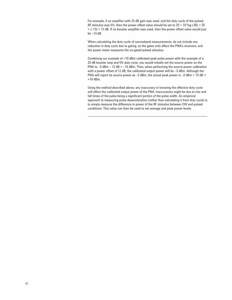
42

For example, if an amplifier with 25 dB gain was used, and the duty cycle of the pulsed-RF stimulus was 5%, then the power offset value should be set to 25 + 10*log (.05) = 25+ (–13) = 12 dB. If no booster amplifier was used, then the power offset value would justbe –13 dB.

When calculating the duty cycle of narrowband measurements, do not include any reduction in duty cycle due to gating, as the gates only affect the PNA’s receivers, andthe power meter measures the un-gated pulsed stimulus.

Combining our example of +10 dBm calibrated peak pulse power with the example of a25 dB booster amp and 5% duty cycle, you would initially set the source power on thePNA to –3 dBm – 12 dB = –15 dBm. Then, when performing the source power calibrationwith a power offset of 12 dB, the calibrated output power will be –3 dBm. Although thePNA will report its source power as –3 dBm, the actual peak power is –3 dBm + 13 dB =+10 dBm.

Using the method described above, any inaccuracy in knowing the effective duty cyclewill affect the calibrated output power of the PNA. Inaccuracies might be due to rise andfall times of the pulse being a significant portion of the pulse width. An empiricalapproach to measuring pulse desensitization (rather than calculating it from duty cycle) isto simply measure the difference in power of the RF stimulus between CW and pulsedconditions. This value can then be used to set average and peak power levels.

43

The last section details the performance differences between the PNA and 8510 networkanalyzers

Figure 46 shows a comparison between the PNA, PNA-L, and the 8510. The 8510’s dominant detection mode is wideband, due to its relatively large bandwidth (about 3 MHzbefore detection, 1.5 MHz for I and Q pulses after detection). The detection is done beforethe analog-to-digital conversion, and is achieved with analog circuitry. The detector consists of a synchronous down-converter which produces baseband I/Q outputs. Pulseprofiling is achieved by varying the sample point along the baseband pulses. The onlyway to trade off speed and dynamic range with the 8510 is with averaging.

The PNA’s dominant detection mode is narrowband, due to its relatively low bandwidthof 35 kHz. All filtering and detection is done after the analog-to-digital conversion, usingdigital-signal processing. Pulse profiling is achieved with analog switches that gate the IF(or RF) signals prior to filtering and detection. The PNA’s narrowband mode trades offspeed and dynamic range using variable IF bandwidths as well as averaging. The PNAcan also do broadband detection with pulses as narrow as 50 us.

The PNA-L’s dominant mode is wideband detection. All filtering and detection is doneafter the analog-to-digital conversion, using digital-signal processing. The widest IF bandwidths are 250 kHz (2-port 20, 40, 50 GHz models) or 600 kHz (2-port 6, 13.5 GHz and4-port 20 GHz models) allowing point-in-pulse measurements of 10 us or 2 us respectively.Pulse profiling is similar to the 8510 except the sampling is done on IF pulses instead ofbaseband pulses. Normally, wideband detection is done at the widest IF bandwidth, sothe only way to improve dynamic range is by averaging.

Although PNA, PNA-L, and 8510-based systems make measurements with different hardware and different types of detection, the resulting pulsed S-parameter and pulse-profile measurements are identical for a given device tested on any of the systems.

Figure 46. Comparing the 8510, PNA, and PNA-L

Comparing the PNA and8510

8510 (85108A)• Dominant mode is wideband detection• Detection is done BEFORE analog-to-digital conversion• Analog synchronous detector produces baseband I/Q

output (detector bandwidth = 1.5 MHz)• Pulse profiling achieved by varying sample point of baseband pulses• Trade off speed and dynamic range with averaging

PNA• Dominant mode is narrowband detection• All processing (filtering and detection) is done digitally• Widest bandwidth = 35 kHz• Pulse profiling achieved with analog switches that gate

IF (or RF) signals• Trade off speed and dynamic range with variable IF

bandwidths and averaging

PNA-L• Dominant mode is wideband detection• All processing (filtering and detection) is done digitally• Widest bandwidth = 250 or 600 kHz• Pulse profiling achieved by varying sample point of IF pulses• Trade off speed and dynamic range with averaging

44

Figure 47 shows the 85108A’s dynamic range versus pulse width for various duty cycles.The data was taken using a constant time-per-point of 90 ms. In some 8510 cases, moreaveraging could be done in this time frame, resulting in increased dynamic range.

Figure 47. 85108A dynamic range versus pulse width for various duty cycles

Figure 48 shows the PNA’s dynamic range versus pulse width for various duty cycles. ThePNA’s bandwidth was 10 Hz, to match the time-per-point of 90 ms used for the 85108Adata.

Figure 48. PNA dynamic range versus pulse width for various duty cycles

40

50

60

70

80

90

100

110

Pulse width (us)

Rece

iver

dyn

amic

rang

e (d

B)

10%

5%

1%

0. 50%

0. 10%

0. 05%

0. 01%

(using wideband detection, effective IF bandwidth = 3 MHz)

0 105 15 20

Number of averages increases to keep constant time-per-point

85108 dynamic range vs. pulse width for duty cyclesfrom 0.01% to 10% (90 ms per point)

PNA dynamic range vs. pulse width for duty cyclesfrom 0.01% to 10% (90 ms per point)

40

50

60

70

80

90

100

110

Pulse width (us)

Rece

iver

dyn

amic

rang

e (d

B)

10%

5%

1%

0. 50%

0. 10%

0. 05%

0. 01%

(using 10 Hz bandwidth)

0 105 15 20

45

Figure 49 shows the actual dynamic range versus duty cycle, between the 8510 and PNA.The bandwidth of the PNA was chosen to give the same time-per-point as the 8510. ThePNA’s dynamic range varies with duty cycle, but the crossover point is at about 0.1% duty cycle. For most radar applications (duty cycles in the 1 to 10% range), the PNA hassuperior dynamic range compared to the 8510.

Figure 49. Comparing dynamic range of the PNA and 8510

Figure 50 shows an example point-in-pulse measurement of a bandpass filter. Althoughfilters are not normally measured under pulse conditions, they are very useful to showthe overall dynamic range of the test system. The pulse conditions used for this examplewere chosen because they are representative of a typical radar application. Note, there isexcellent correlation between the PNA and 8510 in the passband and transition region ofthe filter. This example also shows that the PNA has about 10 dB better dynamic range,and sweeps 6 times faster than the 8510.

Figure 50. Example measurement comparison of PNA and 8510

85108 and PNA dynamic range vs duty cycle (90 ms/point)

0.0

20.0

40.0

60.0

80.0

100.0

120.0

0.01% 0.10% 1.00% 10. 00%

Duty cycle

Dyn

amic

ran

ge (

dB)

20 us

10 us

5 us

2 us

1 us

PNA

8510

PNA

Radar

Pulse width*

* Pulse widths are for the 8510. The PNA's dynamic range is a function of duty cycle, irrespective of pulse width

-1 00

-9 0

-8 0

-7 0

-6 0

-5 0

-4 0

-3 0

-2 0

-1 0

0

7.74

7.99

8.24

8.49

8.74

8.99

9.24

9.49

9.74

9.99

10.2

4

10.4

9

10.7

4

10.9

9

11.2

4

11.4

9

11.7

4

11.9

9

12.2

4

12.4

9

12.7

4

Frequency (GHz)

S2

1 (

dB

)

PN A

8510

8510 sweep time = 9.0 sPNA sweep time = 1.4 s (6x faster)

PW = 5 usPRF = 10 kHzDuty cycle = 5%Points = 2018510: no avgPNA: no avg, BW=567 HzCalibration: 2-port

46

Figure 51 is a review of some of the key issues we have covered in this application note.One thing to note is that the 8510’s narrowband mode is limited to high PRF’s (minimumPRF around 50 kHz to 100 kHz), and no spectral nulling is available.

Figure 51. Pulse summary

Advantages

Disadvantages

8510

PNA/PNA-L

PNA options

Measurements

Wideband/synchronous

Constant dynamic range

Lower pulse width limit

Elevated noise floor

PW > 1 us

PW > 50 us/10 us/2 us**

None required

Average

Point-in-pulse

Pulse profile

Pulse-to-pulse

Narrowband/asynchronous

Narrow pulse widths

Dynamic range loss with

small duty cycles

No pulse-to-pulse

Limited*

PW > 20 ns (limited by IF gate)

H11/H08***

Average

Point-in-pulse

Pulse profile

* Hi PRF, no nulling, no point-in-pulse

** PNA/PNA-L 2-port 20, 40, 50 GHz/PNA-L 2-port 6, 13.5, 4-port 20 GHz

*** Option H08 is usually used in conjunction with Option H11. Without H11, the user can perform average pulse, or point-in-pulse measurements using external RF gates.

47

Testing with pulsed RF stimulus is very important for radar, electronic warfare and wireless communications systems. Modern network analyzers utilize two different detection schemes, each with advantages and disadvantages. Both wideband and narrowband detection can be used for point-in-pulse, and pulse-profile measurements.Pulse-to-pulse measurements require wideband detection. Although wideband detectionhas traditionally been the more widely used technique due to the popularity of pulsed8510 systems, narrowband detection is a powerful alternative for analyzing pulsed-RF signals. Agilent’s unique spectral nulling technique improves measurement speed considerably by using wider IF bandwidths. For radar and wireless communication applications, narrowband detection offers superior dynamic range and speed comparedto the 8510. And with narrowband detection, there is no lower limit to pulse widths.

It is important to remember that although the PNA and PNA-L use different hardware anddetection techniques than the 8510, the measurements and the measurement results areessentially the same – they both provide accurate pulsed-RF S-parameters.

In addition to providing high-quality pulsed-RF S-parameter measurements, the PNA andPNA-L offer many platform benefits. The PNA family has more measurement flexibilitywith 32 measurement channels, 128 traces, 16 windows, and up to 16,001 data points.The PNA family also offers all of the connectivity you’d expect from a PC-based instrument,such as connecting to printers via LAN, and using USB peripherals. Furthermore, theopen Windows® environment allows maximum flexibility for automating measurements,like running software right on the instrument, and using COM and DCOM for fast programexecution and data transfer. The PNA family also has many features to ease the task ofvector network measurements, like a built-in HELP system, Calibration Wizards, and electronic calibration that works up to 67 GHz.

Summary

Web Resources

Pulsed-RF measurements:www.agilent.com/find/pulsedrf

Aerospace & defense applications:www.agilent.com/find/ad

PNA series network analyzers:www.agilent.com/find/pna

Electronic calibration (ECal):www.agilent.com/find/ecal

RF and microwave test accessories:www.agilent.com/find/accessories

Windows® is a U.S. registered trademark of the Microsoft Corporation.

Agilent Email Updates

www.agilent.com/find/emailupdates

Get the latest information on the productsand applications you select.

www.agilent.com/find/agilentdirect

Quickly choose and use your test equipment solutions with confidence.

www.agilent.com/find/open

Agilent Open simplifies the process ofconnecting and programming test systemsto help engineers design, validate andmanufacture electronic products. Agilentoffers open connectivity for a broad rangeof system-ready instruments, open industrysoftware, PC-standard I/O and global support, which are combined to more easily integrate test system development.

Agilent Direct

AgilentOpen

www.agilent.com

For more information on Agilent Technologies’products, applications or services, pleasecontact your local Agilent office. The completelist is available at:

www.agilent.com/find/contactus

Phone or Fax

North AmericaCanada (877) 894-4414Latin America 305 269 7500United States (800) 829-4444

Asia PacificAustralia 1 800 629 485China 800 810 0189Hong Kong 800 938 693India 1 800 112 929Japan 0120 (421) 345Korea 080 769 0800Malaysia 1 800 888 848Singapore 1 800 375 8100Taiwan 0800 047 866Thailand 1 800 226 008

EuropeAustria 0820 87 44 11Belgium 32 (0) 2 404 93 40 Denmark 45 70 13 15 15Finland 358 (0) 10 855 2100France 0825 010 700*

*0.125 fixed network ratesGermany 01805 24 6333**

**0.14/minute

Ireland 1890 924 204Israel 972-3-9288-504/544Italy 39 02 92 60 8484Netherlands 31 (0) 20 547 2111Spain 34 (91) 631 3300Sweden 0200-88 22 55Switzerland (French) 41 (21) 8113811 (Opt 2)Switzerland (German) 0800 80 53 53 (Opt 1)United Kingdom 44 (0) 118 9276201Other European Countries:www.agilent.com/find/contactusRevised: March 24, 2007

Product specifications and descriptions inthis document subject to change withoutnotice.

© Agilent Technologies, Inc. 2006, 2007Printed in USA, November 28, 20075989-4839EN

Remove all doubt

Our repair and calibration services will get your equipment back to you,performing like new, when promised.You will get full value out of yourAgilent equipment throughout itslifetime. Your equipment will be servicedby Agilent-trained technicians using the latest factory calibration procedures,automated repair diagnostics and genuine parts. You will always have theutmost confidence in your measurements.

Agilent offers a wide range of additionalexpert test and measurement servicesfor your equipment, including initialstart-up assistance onsite educationand training, as well as design, systemintegration, and project management.

For more information on repair and calibration services, go to:

www.agilent.com/find/removealldoubt