Aggregate Supply IB Economics

Continued… �  Describe the term aggregate supply.

�  Explain, using a diagram, why the short-run aggregate supply curve (SRAS curve) is upward sloping.

�  Explain, using a diagram, how the AS curve in the short run (SRAS) can shift due to factors including changes in resource prices, changes in business taxes and subsidies and supply shocks.

�  Explain, using a diagram, that the monetarist/new classical model of the long- run aggregate supply curve (LRAS) is vertical at the level of potential output (full employment output) because aggregate supply in the long run is independent of the price level.

�  Explain, using a diagram, that the Keynesian model of the aggregate supply curve has three sections because of “wage/price” downward inflexibility and different levels of spare capacity in the economy.

Continued… �  Explain, using the two models above, how factors

leading to changes in the quantity and/or quality of factors of production (including improvements in efficiency, new technology, reductions in unemployment, and institutional changes) can shift the aggregate supply curve over the long term.

Equilibrium:

�  Explain, using a diagram, the determination of short-run equilibrium, using the SRAS curve.

�  Examine, using diagrams, the impacts of changes in short- run equilibrium.

Continued… �  Explain, using a diagram, the determination of

long-run equilibrium, indicating that long-run equilibrium occurs at the full employment level of output.

�  Explain why, in the monetarist/new classical approach, while there may be short-term fluctuations in output, the economy will always return to the full employment level of output in the long run.

�  Examine, using diagrams, the impacts of changes in the long-run equilibrium.

Continued… �  Explain, using the Keynesian AD/AS diagram, that

�  the economy may be in equilibrium at any level of real output where AD intersects AS.

�  Explain, using a diagram, that if the economy is in equilibrium at a level of real output below the full employment level of output, then there is a deflationary (recessionary) gap.

�  Discuss why, in contrast to the monetarist/new classical model, the economy can remain stuck in a deflationary (recessionary) gap in the Keynesian model.

�  Explain, using a diagram, that if AD increases in the vertical section of the AS curve, then there is an inflationary gap.

�  Discuss why, in contrast to the monetarist/new classical model, increases in aggregate demand in the Keynesian AD/AS model need not

�  be inflationary, unless the economy is operating close to, or at, the level of full employment.

Continued… HL Only �  Explain, with reference to

the concepts of leakages (withdrawals) and injections, the nature and importance of the Keynesian multiplier.

�  Calculate the multiplier using either of the following formulae.

�  1/(1- MPC)

�  1 /(MPS + MPT + MPM)

�  Use the multiplier to calculate the effect on GDP of a change in an injection in investment, government spending or exports.

�  Draw a Keynesian AD/AS diagram to show the impact of the multiplier.

Links to Theory of Knowledge

�  The Keynesian and Monetarist positions differ on the shape of the AS curve.

�  What is needed to settle this question: empirical evidence (if so, what should be measured?), strength of theoretical argument, or factors external to economics such as political conviction?

Introduction to Aggregate Supply

AD- revisited �  As we studied before, AD is the total output

produced in a nation. AD=C+I+G+(X-M)

�  This will affect households, firms and governments budget

�  An increase in output will lead to an outward shift in the AD curve and vise versa

Aggregate Supply: �  Definition:

�  The total output produced by the firms in a nation at a range of price levels in a given period of time.

Similarities to Microeconomics

�  Increase in price levels= increase in output

�  Decrease in price levels= decrease in output

�  (The law of supply)

The Aggregate Supply Curve

�  The aggregate supply curve is generally upward sloping.

�  For our analysis, we will consider the short-run aggregate supply curve and the long-run aggregate supply curve.

PL SRAS

real GDP Yfe

LRAS

Short-run aggregate supply (SRAS):

�  Illustrates the relationship between the price level of a nation’s output and the level of output produces

�  in the fixed-wage and price period, which is the period of time following a change in aggregate demand over which

Long-run aggregate supply (LRAS):

�  Illustrates the relationship between the price level and the level of output

�  in the flexible-wage and price period, which is the period of time following a change in aggregate demand over which all

Test Your Knowledge �  In your groups, Answer the following questions

�  Post on edmodo

�  Refer to googleDocs for appropriate answer

�  Describe the term aggregate supply.

Video �  Watch the Commanding Heights, part 1, up to 38th

min.

�  And complete the work sheet the provided worksheet.

Competing Views of Aggregate Supply

The  neo-­‐classical  View  of  Aggregate  Supply:  

�  The  ver'cal,  LRAS  curve  reflects  the  theories  of  a  school  of  economic  thought  known  as  the  new  (or  neo)-­‐classical  school  of  economics.    

�  read  on  the  neo-­‐classical  views-­‐  (next  slide)  

�  In  the  new-­‐classical  view,  the  aggregate  supply  curve  is  always  VERTICAL   PL

real GDP Yfe

LRAS

Read �  The  Classical  view  of  Aggregate  Supply:  During  the  boom  era  of  the  Industrial  

Revolu'ons  in  Europe,  Britain  and  the  United  States,  governments  played  a  rela'vely  small  role  in  na'on’s  economies.  Economic  growth  was  fueled  by  private  investment  and  consump'on,  which  were  leE  largely  unregulated  and  unchecked  by  government.  When  labor  unions  were  weak  and  minimum  wages  and  unemployment  benefits  were  unheard  of,  wages  fluctuated  depending  on  market  demand  for  labor.  When  spending  in  the  economy  was  strong,  wages  were  driven  up  and  firms  restricted  their  output  in  response  to  higher  costs,  keeping  output  near  the  full  employment  level.  When  spending  in  the  economy  was  weak,  firms  lowered  workers'  wages  without  fear  of  repercussions  from  unions  or  government  requiring  minimum  wages.  Flexible  wages  meant  labor  markets  were  responsive  to  changing  macroeconomic  condi'ons,  and  economies  tended  to  correct  themselves  in  'mes  of  excessively  weak  or  strong  aggregate  demand.    

�  The  Classical  view  of  aggregate  supply  held  that  leE  unregulated,  a  week  or  over-­‐hea'ng  economy  would  "self-­‐correct"  and  return  to  the  full-­‐employment  level  of  output  due  to  the  flexibility  of  wages  and  prices.  When  demand  was  weak,  wages  and  prices  would  adjust  downwards,  allowing  firms  to  maintain  their  output.  When  demand  was  strong,  wages  and  prices  would  adjust  upwards,  and  output  would  be  maintained  at  the  full-­‐employment  level  as  firms  cut  back  in  response  to  higher  costs.    

The  Keynesian  View  of  Aggregate  Supply:  

�  The  upwards  sloping,  SRAS  curve  reflects  the  theories  of  a  school  of  economic  thought  known  as  the  Keynesian  school.  

�  Click here to read on the Keynesian view

�  In the Keynesian view, AS is horizontal below full-employment and vertical beyond full employment!

PL SRAS

real GDP Yfe

Read �  The  Keynesian  View  of  Aggregate  Supply:  John  Maynard  Keynes  was  an  English  

economist  who  represented  the  Bri'sh  at  the  Versailles  treaty  talks  at  the  end  of  WWI.  During  the  Great  Depression,  Keynes  no'ced  that,  in  contrast  to  what  the  neo-­‐classical  economists  thought  should  happen,  the  world’s  economies  were  not  self-­‐correcEng.    

�  Keynes  believed  that  during  a  'me  of  weak  spending  (AD),  an  economy  would  be  unable  to  return  to  the  full-­‐employment  level  of  output  on  its  own  due  to  the  downwardly  inflexible  nature  of  wages  and  prices.  Since  workers  would  be  unwilling  to  accept  lower  nominal  wages,  and  because  of  the  role  unions  and  the  government  played  in  protec'ng  worker  rights,  the  only  thing  firms  could  due  when  demand  was  weak  was  decrease  output  and  lay  off  workers.  As  a  result,  a  fall  in  aggregate  demand  below  the  full-­‐employment  level  results  in  high  unemployment  and  a  large  fall  in  output.  To  avoid  deep  recession  and  rising  unemployment  aEer  a  fall  in  private  spending  (C,  I,  Xn),  a  government  must  fill  the  "recessionary  gap"  by  increasing  government  spending.  The  economy  will  NOT  "self-­‐correct"  due  to  "s'cky  wages  and  prices",  meaning  there  should  be  an  ac've  role  for  government  in  maintaining  full-­‐employment  output.  

AS Curves

The Classical view PL

real GDP

AS

Yfe

The Keynesian view PL

real GDP

AS

Yfe

�  In reality, neither view is totally correct.

•  Keynes was right in the short-run, because wages and prices tend not to adjust quickly to changes in the level of demand.

•  The new-classical are right in the long-run, because over time, following a decrease or an increase in AD, wages and prices tend to rise or fall accordingly.

•  causing output in the nation to return to a relatively constant, full-employment level, regardless of the level of AD.

Discussion: �  Discuss with your partner and answer the following

question:

�  Why does the SRAS curve slopes upward? Why does the LRAS curve is vertical?

�  Post your answer on Edmodo

Test Your Knowledge �  In your groups, answer the following questions

�  Post your answers on edmodo

�  Refer to googleDocs for appropriate answers

�  Explain, using a diagram, that the monetarist/new classical model of the long- run aggregate supply curve (LRAS) is vertical at the level of potential output (full employment output) because aggregate supply in the long run is independent of the price level.

�  Explain, using a diagram, that the Keynesian model of the aggregate supply curve has three sections because of “wage/price” downward inflexibility and different levels of spare capacity in the economy.

Short-run Aggregate Supply

�  The  Keynesian  theory  of  rela'vely  inflexible  wages  and  prices  is  reflected  in  the  short-­‐run  aggregate  supply  curve    

�  which  is  rela'vely  flat  below  full  employment  (Yfe)  and  rela'vely  steep  beyond  full  employment.  

Explanation for the shape of SRAS

�  Slopes upwards because at higher prices, firms respond by producing a greater quantity of output

�  As price level falls, firms respond by reducing output

�  At low levels of output (when unemployment is high), firms are able to attract new workers without paying higher wages, so prices rise gradually as output increases

�  At high levels of output, when resources in the economy are fully employed, firms find it costly to increase output as they must pay higher wages and other costs.

�  Increases in output are accompanied by greater and greater levels of inflation as an economy approaches and passes full employment

�  See the graph in the next slide

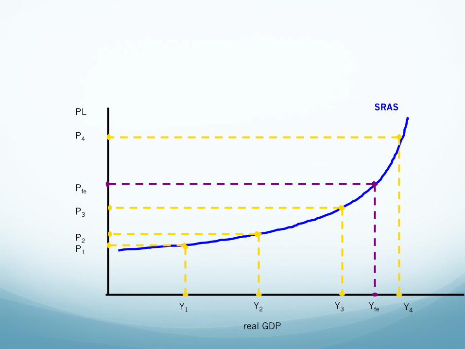
PL SRAS

P1

P2

P3

P4

Y1 Y2 Y3 Y4

real GDP

Pfe

Yfe

Long-run Aggregate Supply

�  The  new-­‐classical  view  of  AS  is  reflected  in  the  ver'cal,  long-­‐run  AS  curve,  which  shows  that  output  will  always  occur  at  the  full  employment  level  (Yfe).  

Explanation for the shape of LRAS

�  AS is vertical at the full-employment level of output (Yfe),

�  implying that whatever the level of AD, the economy will always produce at full employment.

�  When AD is very low, wages and prices fall so that firms can continue to employ the same number of workers and produce the same output.

�  Output will not decrease when AD decreases

�  When AD is very high, firms will see wages rising and therefore they will NOT hire more workers,

�  and will just pass their higher costs onto buyers as higher prices.

�  Output will not increase when AD increases

�  Wages and prices must be completely flexible in the long-run for Yfe to always prevail

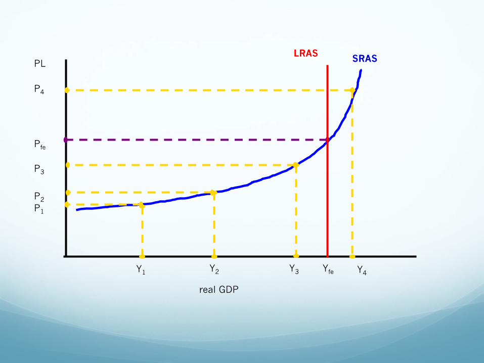
PL SRAS

P1

P2

P3

P4

Y1 Y2 Y3 Y4

LRAS

real GDP

Pfe

Yfe

Discussion �  With your partner, distinguish between the SRAS

and LRAS

The Determinants of Aggregate Supply

�  A  change  in  AD  is  not  the  only  factor  that  can  lead  to  a  change  in  an  economy’s  short-­‐run  equilibrium  level  of  output.  

�   AS  can  also  shiE,  if  one  of  the  determinants  of  aggregate  supply  changes.  

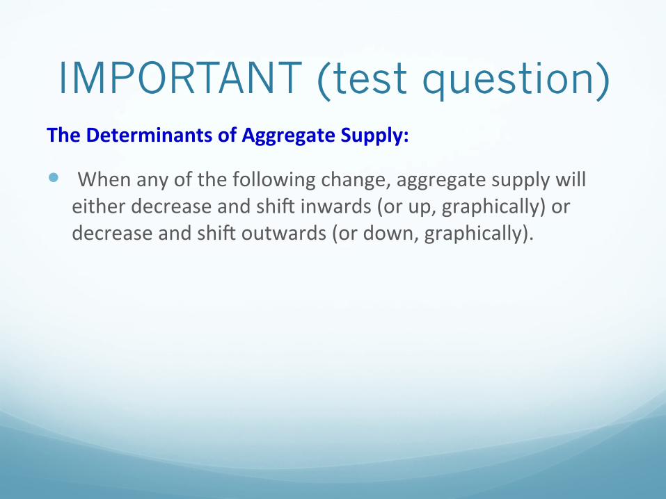
IMPORTANT (test question) The  Determinants  of  Aggregate  Supply:  

�   When  any  of  the  following  change,  aggregate  supply  will  either  decrease  and  shiE  inwards  (or  up,  graphically)  or  decrease  and  shiE  outwards  (or  down,  graphically).  

�  Wage  rates:  The  cost  of  labor.  Higher  wages  cause  SRAS  to  decrease,  lower  wages  cause  SRAS  to  increase  

•  Resource  costs:  Rents  for  land,  interest  on  capital;  as  these  rise  and  fall,  so  does  AS  

•  Energy  and  transportaBon  costs:  Higher  oil  or  energy  prices  will  cause  SRAS  to  decrease.  If  costs  fall,  SRAS  increases  

�  Government  regulaBon:  Regula'ons  impose  costs  on  firms  that  can  cause  SRAS  to  decrease  

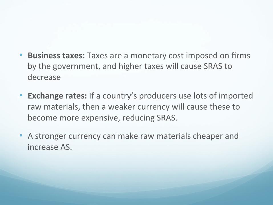
•  Business  taxes:  Taxes  are  a  monetary  cost  imposed  on  firms  by  the  government,  and  higher  taxes  will  cause  SRAS  to  decrease  

•  Exchange  rates:  If  a  country’s  producers  use  lots  of  imported  raw  materials,  then  a  weaker  currency  will  cause  these  to  become  more  expensive,  reducing  SRAS.    

•  A  stronger  currency  can  make  raw  materials  cheaper  and  increase  AS.

Short-run Equilibrium in the AD/AS Model – Full Employment

�  By  considering  both  the  aggregate  supply  AND  the  aggregate  demand  in  a  na'on,  

�   we  can  analyze  the  levels  of  output,  employment  and  prices  in  an  economy  at  any  par'cular  period  of  'me

PL SRAS LRAS

real GDP

Pfe

Yfe

AD1

Consider  the  economy  shown  here:

When equilibrium occurs at full-employment:

•  The total demand for the nation’s output is just high enough for the economy to produce at its full employment level in the short-run.

•  Nearly everyone who wants a job has a job and the nation’s capital and land are being fully utilized. Unemployment is at its Natural Rate (the NRU)

•  (frictional + structural unemployment) / labor force

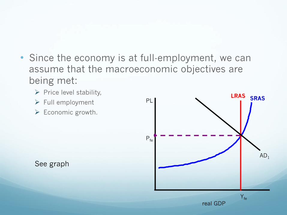
•  Since the economy is at full-employment, we can assume that the macroeconomic objectives are being met: Ø  Price level stability,

Ø  Full employment

Ø  Economic growth.

PL SRAS LRAS

real GDP

Pfe

Yfe

AD1

See graph

What happens if the AD falls?

Short-run Equilibrium in the AD/AS Model – AD decreases

�  On  the  previous  slide  we  say  an  economy  that  was  producing  at  its  full  employment  level,  e.g.  a  strong,  healthy  economy.    

�  But  what  if  something  changed,  and  AD  fell  due  to  a  fall  in  consumpEon,  net  exports,  investment  or  government  spending?

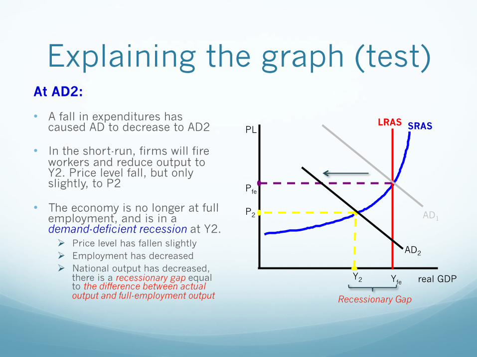
Explaining the graph (test) At AD2:

•  A fall in expenditures has caused AD to decrease to AD2

•  In the short-run, firms will fire workers and reduce output to Y2. Price level fall, but only slightly, to P2

•  The economy is no longer at full employment, and is in a demand-deficient recession at Y2. Ø  Price level has fallen slightly Ø  Employment has decreased Ø  National output has decreased,

there is a recessionary gap equal to the difference between actual output and full-employment output

PL SRAS LRAS

real GDP

Recessionary Gap

Pfe

Yfe

P2

Y2

AD1

AD2

What happens when the AD decreases in the LR

equilibrium?

Long-run Equilibrium in the AD/AS Model: AD decreases

�  When  AD  decreases,  output  will  decrease  in  the  short-­‐run  because  firms  will  have  to  lay  workers  off  to  cut  costs  and  lower  their  prices.  

�   However,  in  the  long-­‐run,  wages  and  prices  are  flexible,  so  output  will  return  to  its  full  employment  level.

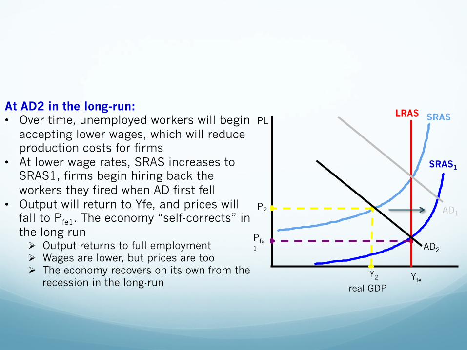
At AD2 in the long-run: •  Over time, unemployed workers will begin

accepting lower wages, which will reduce production costs for firms

•  At lower wage rates, SRAS increases to SRAS1, firms begin hiring back the workers they fired when AD first fell

•  Output will return to Yfe, and prices will fall to Pfe1. The economy “self-corrects” in the long-run Ø  Output returns to full employment Ø  Wages are lower, but prices are too Ø  The economy recovers on its own from the

recession in the long-run

PL SRAS LRAS

SRAS1

real GDP

Pfe1

Yfe

P2

Y2

AD1

AD2

What happens when the AD increases in the SR

equilibrium?

Short-run Equilibrium in the AD/AS Model – AD increases

�  Assume  that  either  consumpEon,  investment,  net  exports  or  government  spending  increased,  causing  the  AD  curve  to  shiE  from  AD1  to  AD3

PL SRAS LRAS

real GDP

Pfe

Yfe

P3

Y3

AD1

AD3

Inflationary Gap

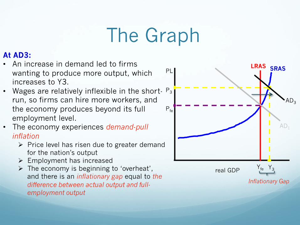
The Graph At AD3: •  An increase in demand led to firms

wanting to produce more output, which increases to Y3.

•  Wages are relatively inflexible in the short-run, so firms can hire more workers, and the economy produces beyond its full employment level.

•  The economy experiences demand-pull inflation Ø  Price level has risen due to greater demand

for the nation’s output Ø  Employment has increased Ø  The economy is beginning to ‘overheat’,

and there is an inflationary gap equal to the difference between actual output and full-employment output

PL SRAS LRAS

real GDP

Pfe

Yfe

P3

Y3

AD1

AD3

Inflationary Gap

What happens when the AD increases in the LR

equilibrium?

Long-run Equilibrium in the AD/AS Model – AD increases

�  In  the  long-­‐run,  wages  and  prices  will  adjust  to  the  level  of  aggregate  demand  in  the  economy.    

�  When  AD  grows  beyond  the  full  employment  level,  this  means  wages  will  rise  in  the  long-­‐run  

�  leading  producers  to  reduce  employment  and  output  back  to  the  full-­‐employment  level

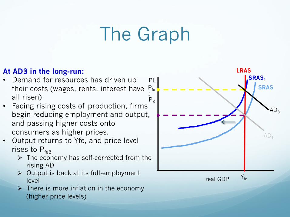
The Graph

PL SRAS

LRAS SRAS1

real GDP

Pfe3

Yfe

P3

AD1

AD3

At AD3 in the long-run: •  Demand for resources has driven up

their costs (wages, rents, interest have all risen)

•  Facing rising costs of production, firms begin reducing employment and output, and passing higher costs onto consumers as higher prices.

•  Output returns to Yfe, and price level rises to Pfe3 Ø  The economy has self-corrected from the

rising AD Ø  Output is back at its full-employment

level Ø  There is more inflation in the economy

(higher price levels)

More stuff on AS Almost done, I promise

Negative Supply Shocks -Stagflation-

�  Assume  that  a  determinant  of  AS  changes  which  causes  the  short-­‐run  aggregate  supply  curve  to  decrease,  and  shiE  to  the  leE.    

�  What  results  is  a  situa'on  known  as  stagfla&on

�  DEFENIITON: Stagflation, An increase in the average price level combined with a decrease in output, caused by a negative supply shock.

�  “Stagnant growth” and “inflation” together make “stagflation”

The Graph

PL

SRAS1

LRAS SRAS2

real GDP

Pfe

Yfe

P2

Y2

AD

•  Assume higher energy costs caused SRAS to decrease to SRAS2.

•  To off-set higher energy costs, firms must lay off workers, reducing employment.

•  Higher costs must be passed onto consumer as higher prices, causing inflation.

•  An economy facing stagflation will only self-correct if resources costs fall in the long-run, which may occur if wages fall due to a large increase in unemployment.

Positive Supply Shock -Economic Growth-

�  While  a  nega've  supply  shock  can  be  disastrous  for  an  economy,  a  posi've  supply  shock  has  very  beneficial  effects  on  employment,  output  and  the  price  level.  

�   Assume  ,for  example,  a  na'on  signs  a  free  trade  agreement  and  now  lots  of  new  resources  can  be  imported  at  very  low  costs.

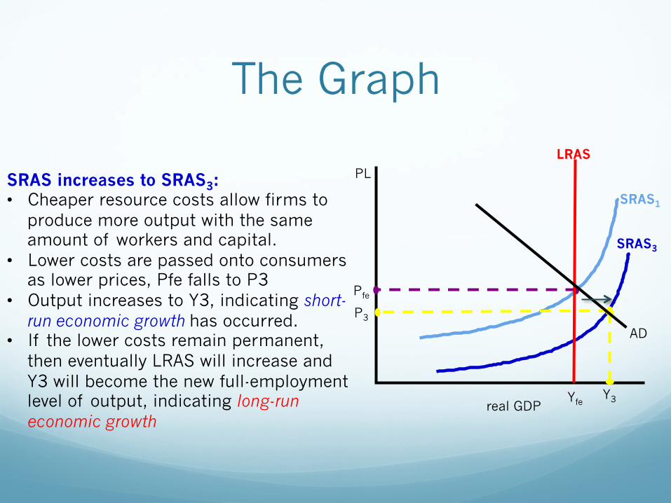
The Graph

SRAS increases to SRAS3: •  Cheaper resource costs allow firms to

produce more output with the same amount of workers and capital.

•  Lower costs are passed onto consumers as lower prices, Pfe falls to P3

•  Output increases to Y3, indicating short-run economic growth has occurred.

•  If the lower costs remain permanent, then eventually LRAS will increase and Y3 will become the new full-employment level of output, indicating long-run economic growth

PL

SRAS3

LRAS

SRAS1

real GDP

Pfe

Yfe

P3

Y3

AD

Long-run Economic Growth in the AD/AS Model

�  So  far  we  have  illustrated  demand-­‐deficient  recessions,  demand-­‐pull  inflaEon,  negaEve  and  posiEve  supply  shocks.    

�  But  real,  long-­‐run  economic  growth  requires  that  not  only  AS  or  AD  increase,  rather  that  both  AS  AND  AD  increase.  

The Graph

PL

SRAS2

LRAS1

SRAS1

LRAS2

real GDP

Pfe

Yfe1 Yfe2

AD1 AD2

Long-run Economic Growth: •  For national output to grow in the

long-run, AD, SRAS and LRAS must all shift outward.

•  This can be cause by an improvement in the production possibilities of the nation, combined with growing demand for the nation’s output.

•  The quality and/or quantity of resources must increase: Ø  Better technology, Ø  Larger population, Ø  Better educated workforce, Ø  More natural resources, and so on.

Video �  Watch the Video and answer the following

questions on edmodo

�  Refer to googleDocs for appropreate answer

�  http://www.econclassroom.com/?p=2807

Test Your Knowledge �  Explain, using a diagram, the determination of short-run equilibrium,

using the SRAS curve.

�  Examine, using diagrams, the impacts of changes in short- run equilibrium.

�  Explain, using a diagram, the determination of long-run equilibrium, indicating that long-run equilibrium occurs at the full employment level of output.

�  Explain why, in the monetarist/new classical approach, while there may be short-term fluctuations in output, the economy will always return to the full employment level of output in the long run.

�  Examine, using diagrams, the impacts of changes in the long-run equilibrium.

HWK.. Test Prep �  Practice questions:

�  IB Econ, Jason Welker �  Page 284