Embed Size (px)
DESCRIPTION
High explosives can be used to aerosolize and disperse a variety of hazardous materials. The rate at which those materials would settle out of the atmosphere, though, is dependent on their size distribution.In experimental work, it was discovered that there is actually a profound, two-way relationship between the fireball and the particles entrained within it, as it also provides the turbulent, high temperature environment that drives particle interactions, allowing them to agglomerate and deposit onto one another. These actually serve to increase overall particle size, so that less material remains aerosol-sized. In addition, the entrainment of soil provides additional sites with which the hazardous particulates interact, and thus enhances agglomeration.Significant secondary effects exist in the fireball, therefore, that influence the amount of material that can be released into the air as aerosols, and thus reduce the amount of hazardous material that can be suspended and transported in the atmosphere.
Citation preview
AEROSOLIZATION AND SOIL ENTRAINMENT INEXPLOSIVE FIREBALLS
AEROSOLISATION ET L’ENTRAINMENT DU SOLDANS LES EXPLOSIONS
A Thesis Submittedto the Division of Graduate Studies of the Royal Military College of Canada
by
Luke Simon Lebel
In Partial Fulfillment of the Requirements for the Degree ofDoctor of Philosophy
October, 2012
©This thesis may be used within the Department of National Defence butcopyright for open publication remains the property of the author

ii
ROYAL MILITARY COLLEGE OF CANADACOLLEGE MILITAIRE ROYAL DU CANADA
DIVISION OF GRADUATE STUDIES AND RESEARCHDIVISION DES ETUDES SUPERIEURES ET DE LA RECHERCHE
This is to certify that the thesis prepared by / Ceci certifie que la these redigee par
LUKE SIMON LEBEL
entitled / intitulee
AEROSOLIZATION AND SOIL ENTRAINMENT IN EXPLOSIVEFIREBALLS
AEROSOLISATION ET L’ENTRAINMENT DU SOL DANS LESEXPLOSIONS
complies with the Royal Military College of Canada regulations and that it meetsthe accepted standards of the Graduate School with respect to quality, and, in thecase of a doctoral thesis, originality, / satisfait aux reglements du College militaireroyal du Canada et qu’elle respecte les normes acceptees par la Faculte des etudessuperieures quant a la qualite et, dans le cas d’une these de doctorat, l’originalite,
for the degree of / pour le diplome de
DOCTOR OF PHILOSOPHY IN NUCLEAR ENGINEERING
Signed by the final examining committee: / Signe par les membres du comiteexaminateur de la soutenance de these
,Chair / President
, External Examiner / Examinateur externe
, Main Supervisor / Directeur de these principal
Approved by the Head of Department : /Approuve par le Directeur du Departement: Date:
To the Librarian: This thesis is not to be regarded as classified. / AuBibliothecaire : Cette these n’est pas consideree comme a publication restreinte.
Main Supervisor / Directeur de these principal
iii

iv

To Nikki and Isaac,
v

vi
Acknowledgements
My work would not have been possible without the support of many different in-
dividuals, and most of all, my supervisor, Dr. William Andrews. He offered all
the support I needed, but always while pushing me to grow as an independent re-
searcher. For the countless opportunities, for his unwavering belief in me, and for
the way that he saw me as more than just a student, I owe him my sincere thanks.
The detonation calorimetry experiments could not have been carried out without
the hundreds of hours put in Sgt. Eric Lebreton and Don Breen, the ammunition
technicians at CFB Kingston, and two of the nicest and most capable guys in DND.
Nor could my work have been done without Patrick Brousseau, who loaned us the
calorimeter from DRDC Valcartier, and let me piggy back my open air tests on some
of his trials. I am grateful for all his help, along with the phenomenal support I
received in Valcartier from Jean Beaupre and Denis Desrosiers.
The Department of Chemistry and Chemical Engineering at RMC is blessed
with many great technicians, many of whom supported my work directly. Thank
you to Dr. Jennifer Snelgrove, Kathy Nielsen, Kristine Mattson, Brent Ball, Clarence
McEwen, and John Perrault. Thank you also to Dr. Edward Waller and Sharman
Perera from the University of Ontario Institute of Technology for the use of their
particle size measurement equipment.
I would also like to thank all the friends I have made at RMC, who really made
the whole experience of grad school an amazing one. My greatest appreciation,
though, goes to my wife, Nikki, and son, Isaac, to whom I dedicate this work.
This research was funded through the CBRNE Research and Technology Initia-
tive, offered by the DRDC Centre for Security Studies, and through the Director
General Nuclear Safety. In addition, I held the CGS-M and PSGS-D scholarships
from the Natural Science and Engineering Research Council.
vii

viii
Abstract
Lebel, Luke Simon, Ph.D. (Nuclear Engineering). Royal Military College of Canada,
August 2012. Aerosolization and soil entrainment in explosive fireballs, supervised
by Dr. William S. Andrews.
High explosives can be used to aerosolize and disperse a variety of hazardous
materials. The rate at which those materials would settle out of the atmosphere,
though, is dependent on their size distribution. Larger particles, therefore, would
cause high level, but much more localized contamination, where with the aerosol-
sized fraction, contamination would be more diffuse, but also much more widespread.
Two sets of experiments have been employed to study explosive aerosolization,
and to characterize the thermochemical environment in the fireball to which partic-
ulates are exposed. Detonation calorimetry experiments involved detonating small
explosive charges in a closed vessel, measuring the amount of heat that was released
with different oxygen/nitrogen ratios in the vessel, and characterizing the resulting
size distributions and the dispersion of a powdered La2O3 target throughout dif-
ferent types of soil. Open air trials employed a custom-built, fiber optic probe to
sample the light emissions from the interior of a fireball in order to characterize the
evolution of its thermal environment over time.
The experimental work has identified that for particulates, likely because their
mass and inertia allows them deviate from the streamlines of a circulating fluid, their
combustion in the turbulent fireball plays a more important role than the combustion
of gas species. Thermochemical evidence from the calorimetry experiments supports
this, and has found that condensed phase detonation products (as well as entrained
black earth, when present), actually react much faster than gaseous species.
There is actually a profound, two-way relationship between the fireball and the
particles entrained within it, as it also provides the turbulent, high temperature
ix
environment that drives particle interactions, allowing them to agglomerate and de-
posit onto one another. These actually serve to increase overall particle size, so that
less material remains aerosol-sized. In addition, the entrainment of soil provides
additional sites with which the hazardous particulates interact, and thus enhances
agglomeration. Significant secondary effects exist in the fireball, therefore, that in-
fluence the amount of material that can be released into the air as aerosols, and thus
reduce the amount of hazardous material that can be suspended and transported in
the atmosphere.
Keywords: explosive dispersal, fireball mechanics, combustion, thermochem-
istry, aerosols, agglomeration, soil entrainment, calorimetry, spectroscopy
x
Resume
Lebel, Luke Simon, doctorat (genie nucleaire). College militaire royal du Canada,
aout 2012. Aerosolisation et l’entraıment du sol dans les explosions, supervise par
le Dr. William S. Andrews.
Les explosifs peuvent etre utilises pour aerosoliser et disperser une variete de
materes dangereuses. Les contaminants se disperseraient dans l’atmosphere, mais la
distance qu’ils pourraient voyager dependra de la taille des particules. En consequent,
les plus grosses particules causeraient une contamination plus intense, mais beau-
coup plus localisee. En contrepartie, les plus petites particules causeraient une
contamination plus diffuse, mais beaucoup plus repandue.
Deux series d’experiences ont ete utilisees pour etudier l’aerosolisation provenant
des explosifs, et pour caracteriser l’environnement thermochimique dans la boule
de feu a laquelle les particules sont exposees. Les experiences calorimetriques ont
utilise des charges explosives dans un contenant ferme afin de mesurer la quantite de
chaleur liberee selon differentes quantites d’oxygene et d’azote, et pour caracteriser
la taille des particules et la dispersion de poudre de La2O3 dans differents types de
sols. Les essais a l’air libre ont utilise un detecteur a fibre optique afin d’obtenir
les emissions de lumiere qui provenaient de l’interieur de la boule de feu et ainsi
caracteriser l’evolution de l’environnement thermique en fonction du temps.
Les experiences ont revele que la combustion des particules dans la turbulence
d’une boule de feu est plus importante que la combustion des especes gazeuses. Ce
phenomene est probablement du a la masse des particules et leur inertie qui leur
permet de se deplacer dans un fluide en mouvement. Des preuves thermochimiques
des experiences calorimetriques corroborent cette interpretation, ou les produits de
detonation dans la phase condensee (ainsi que de la terre noire, lorsquelle est en-
traınee), reagissent beaucoup plus rapidement que les especes gazeuses.
xi
Il existe un lien bidirectionnel entre la boule de feu et les particules entraınees a
l’interieure de cette derniere, etant donne quelle fournit la turbulence et l’environnement
a haute temperature qui favorisent les interactions entre les particules, leur perme-
ttant alors de s’agglomerer et de se deposer les uns sur les autres. Ces mecanismes
servent a augmenter la taille generale des particules, ce qui reduit la matiere ayant
la taille d’un aerosol. De plus, l’entraınement du sol offre plus de sites ou les partic-
ules dangereuses peuvent interagir, favorisant ainsi l’agglomeration. Donc, des effets
secondaires importants existent dans la boule de feu et ils influencent la quantite
de substances qui peuvent etre emises dans l’air sous forme d’aerosols. Ces effets
peuvent aussi reduire la quantite de contaminants qui peuvent etre suspendus et
propages dans l’atmosphere.
Mots-cles: dispersion explosive, la mecanique de la boule de feu, la combustion,
thermochimie, les aerosols, l’agglomeration, l’entraınement du sol, la calorimetrie,
spectroscopie
xii
Contents
Acknowledgements vii
Abstract ix
Resume xi
List of Tables xvii
List of Figures xix
List of Symbols and Abbreviations xxv
1 Introduction 1
2 Literature Review 5
2.1 Dispersal Devices . . . . . . . . . . . . . . . . . . . . . . . . . . . . . 5
2.2 Explosive Aerosolization . . . . . . . . . . . . . . . . . . . . . . . . . 7
2.3 Particle Agglomeration . . . . . . . . . . . . . . . . . . . . . . . . . . 9
2.4 Fireball Mechanics . . . . . . . . . . . . . . . . . . . . . . . . . . . . 13
2.5 Atmospheric Aerosol Transport . . . . . . . . . . . . . . . . . . . . . 17
3 Experimental Approach 21
3.1 General Approach . . . . . . . . . . . . . . . . . . . . . . . . . . . . 21
3.2 Closed Vessel Detonation Calorimetry Studies . . . . . . . . . . . . . 22
3.2.1 Explosives . . . . . . . . . . . . . . . . . . . . . . . . . . . . . 24
3.2.2 Calorimetry . . . . . . . . . . . . . . . . . . . . . . . . . . . . 24
3.2.3 Residual Solids Analysis . . . . . . . . . . . . . . . . . . . . . 30
3.2.4 Elemental Composition Analysis and Lanthanum Oxide Tracer 31
3.3 Fireball Temperature Studies . . . . . . . . . . . . . . . . . . . . . . 32
3.3.1 Spectroscopic Measurement System . . . . . . . . . . . . . . 32
3.3.2 Experimental Procedure . . . . . . . . . . . . . . . . . . . . . 34
4 Particle Breakup and Growth Mechanisms 35
4.1 Particle Combustion . . . . . . . . . . . . . . . . . . . . . . . . . . . 35
4.2 Mechanical Mechanisms . . . . . . . . . . . . . . . . . . . . . . . . . 37
4.3 Particle Interactions . . . . . . . . . . . . . . . . . . . . . . . . . . . 40
4.4 Summary . . . . . . . . . . . . . . . . . . . . . . . . . . . . . . . . . 43
xiii
5 Explosion Thermochemistry 455.1 Thermochemical Model of an Explosion . . . . . . . . . . . . . . . . 45
5.1.1 General Description . . . . . . . . . . . . . . . . . . . . . . . 455.1.2 Thermochemical Prediction Using CHEETAH Code . . . . . 475.1.3 Thermochemical Model of Secondary Combustion . . . . . . 50
5.2 Calorimetry Results . . . . . . . . . . . . . . . . . . . . . . . . . . . 565.2.1 Calibration of the Detonation Calorimeter . . . . . . . . . . . 565.2.2 Calorimetry of Auxiliary Material . . . . . . . . . . . . . . . 565.2.3 Calorimetry Measurements . . . . . . . . . . . . . . . . . . . 59
5.3 Detonation Product Combustion . . . . . . . . . . . . . . . . . . . . 615.3.1 Computing χ and η from data . . . . . . . . . . . . . . . . . 615.3.2 Applying Thermochemical Model to Data . . . . . . . . . . . 635.3.3 Addition of External Combustible Material . . . . . . . . . . 71
5.4 Results from Fireball Emission Spectral Analysis . . . . . . . . . . . 735.4.1 Time Behaviour . . . . . . . . . . . . . . . . . . . . . . . . . 745.4.2 Fireball Emission Spectra and Estimated Temperatures . . . 765.4.3 Relationship with Fireball Thermochemistry . . . . . . . . . 80
5.5 Extension of Thermochemical Model to Heat Release . . . . . . . . . 825.6 Summary . . . . . . . . . . . . . . . . . . . . . . . . . . . . . . . . . 83
6 Aerosolization 856.1 Results from Residual Solids Analysis . . . . . . . . . . . . . . . . . 86
6.1.1 Laser Diffraction EPCS Results . . . . . . . . . . . . . . . . . 866.1.2 Sieve Analysis Results . . . . . . . . . . . . . . . . . . . . . . 896.1.3 Construction of Particle Size Distributions . . . . . . . . . . . 906.1.4 Degree of Agglomeration . . . . . . . . . . . . . . . . . . . . . 966.1.5 Lanthanum Composition Analysis . . . . . . . . . . . . . . . 100
6.2 Particulates Generated by Explosives . . . . . . . . . . . . . . . . . . 1036.3 Effects on the Particle Size Distributions of Soil . . . . . . . . . . . . 108
6.3.1 Coarse Sand . . . . . . . . . . . . . . . . . . . . . . . . . . . 1116.3.2 Fine Sand . . . . . . . . . . . . . . . . . . . . . . . . . . . . . 1216.3.3 Black Earth . . . . . . . . . . . . . . . . . . . . . . . . . . . . 1286.3.4 Clay . . . . . . . . . . . . . . . . . . . . . . . . . . . . . . . . 135
6.4 Dispersion of a Powdered Target Material . . . . . . . . . . . . . . . 1446.4.1 Coarse Sand . . . . . . . . . . . . . . . . . . . . . . . . . . . 1496.4.2 Fine Sand . . . . . . . . . . . . . . . . . . . . . . . . . . . . . 1526.4.3 Black Earth . . . . . . . . . . . . . . . . . . . . . . . . . . . . 1536.4.4 Clay . . . . . . . . . . . . . . . . . . . . . . . . . . . . . . . . 155
6.5 Summary . . . . . . . . . . . . . . . . . . . . . . . . . . . . . . . . . 157
7 Summary and Conclusions 1617.1 Summary . . . . . . . . . . . . . . . . . . . . . . . . . . . . . . . . . 1617.2 Recommendations and Future Work . . . . . . . . . . . . . . . . . . 164
Bibliography 169
Appendix A 175
Appendix B 179
xiv

Appendix C 191
Appendix D 193
Appendix E 197
Appendix F 199
Appendix G 209
Curriculum Vitae 211
xv

xvi
List of Tables
2.1 List of radioisotopes that pose a security concern, modified from Fer-guson and Smith (2009) . . . . . . . . . . . . . . . . . . . . . . . . . 6
3.1 Experimental design for trials carried out without La2O3 powder . . 243.2 Slopes and intercepts of the pre-detonation and post-detonation in-
tervals . . . . . . . . . . . . . . . . . . . . . . . . . . . . . . . . . . 28
5.1 Thermochemical parameters of C-4 explosive (Fried and Souers, 1994;Cooper, 1996; Liley et al., 1997) . . . . . . . . . . . . . . . . . . . . 48
5.2 Thermochemical parameters of detasheet explosive (Fried and Souers,1994; Cooper, 1996; Liley et al., 1997) . . . . . . . . . . . . . . . . . 49
5.3 Combustion parameters obtained from data . . . . . . . . . . . . . . 675.4 Heats of reaction per mole of oxygen consumed for various compo-
nents . . . . . . . . . . . . . . . . . . . . . . . . . . . . . . . . . . . 68
6.1 Lanthanum concentration in explosive soot and ash residue . . . . . 1006.2 Lanthanum concentration in soot and ash, from the < 250 µm fraction 1086.3 Empirical expressions for coarse sand particle size distributions . . . 1586.4 Empirical expressions for fine sand particle size distributions . . . . 1586.5 Empirical expressions for black earth particle size distributions . . . 1586.6 Empirical expressions for clay particle size distributions . . . . . . . 159
xvii

xviii
List of Figures
2.1 Shock-induced aerosolization mechanisms and how they affect particlesize, taken from Harper et al. (2007) . . . . . . . . . . . . . . . . . . 8
2.2 Explosive fireballs generated from (left to right) nitromethane-zirconium,ALEX (aluminized ammonium nitrate), sensitized nitromethane show-ing interfacial instability and turbulent mixing, taken from Frost et al.(2005) . . . . . . . . . . . . . . . . . . . . . . . . . . . . . . . . . . . 16
2.3 Atmospheric aerosol residence time and deposition velocity, takenfrom Friedlander (2000) . . . . . . . . . . . . . . . . . . . . . . . . . 18
3.1 Schematic of the detonation calorimeter . . . . . . . . . . . . . . . . 25
3.2 Control and data acquisition electronics . . . . . . . . . . . . . . . . 26
3.3 Phases of the temperature profile, including linear pre-detonation andpost-detonation interval from which calculations are taken . . . . . . 27
3.4 Assembly of fiber optic probe for measuring the emission spectra froman explosive fireball . . . . . . . . . . . . . . . . . . . . . . . . . . . 33
3.5 Detonics bay . . . . . . . . . . . . . . . . . . . . . . . . . . . . . . . 34
4.1 SEM micrographs of explosive residue for shots carried out (a) in theabsence of oxygen and (b) in the presence of oxygen . . . . . . . . . 36
4.2 SEM micrographs of black earth, comparing (a) the control blackearth to residual solids collected after shots carried out (b) in theabsence of oxygen and (c) in the presence of oxygen . . . . . . . . . 38
4.3 SEM micrographs of fracturing, comparing (a) the control fine sandto fine sand collected after shots carried out (b) in the absence ofoxygen and (c) in the presence of oxygen . . . . . . . . . . . . . . . 39
4.4 SEM micrographs of agglomeration, comparing (a) the control coarsesand to coarse sand collected after shots carried out (b) in the absenceof oxygen and (c) in the presence of oxygen . . . . . . . . . . . . . . 41
4.5 SEM micrographs of agglomeration, comparing (a) the control clayto residual solids collected after shots carried out (b) in the absenceof oxygen and (c) in the presence of oxygen . . . . . . . . . . . . . . 42
5.1 After compression by the detonation wave, high explosives convert todetonation products, which then expand out into the surroundings;p-v diagram modified from Cooper (1996) . . . . . . . . . . . . . . . 46
5.2 Calibration curve from benzoic acid calibrations for the detonationcalorimeter . . . . . . . . . . . . . . . . . . . . . . . . . . . . . . . . 57
5.3 Calibration curve from benzoic acid calibrations for the Parr Instru-ments model 1241 adiabatic oxygen bomb calorimeter . . . . . . . . 58
xix
5.4 Trials to determine gun tape heat of combustion . . . . . . . . . . . 58
5.5 Trials to determine black earth heat of combustion . . . . . . . . . . 59
5.6 Energy release from explosives as a function of the initial oxygenpartial pressure . . . . . . . . . . . . . . . . . . . . . . . . . . . . . . 60
5.7 Plot of energy-weighted total reaction extent versus the oxygen-weightedtotal reaction extent for C-4 and detasheet trials (point at (1.17,0.67)is an outlier, corresponds to trial DS1215) . . . . . . . . . . . . . . 62
5.8 Piecewise linear fit to the weighted total reaction extent data . . . . 64
5.9 Extent for gas phase and condensed phase reactions . . . . . . . . . 69
5.10 Evolution of Kelvin-Hemholtz instability causing mixing in turbulentshear flow; from Krasny (1986) . . . . . . . . . . . . . . . . . . . . . 70
5.11 Particles have inertia, and do not exactly follow the streamlines ofthe carrier gas . . . . . . . . . . . . . . . . . . . . . . . . . . . . . . 71
5.12 Linear fit to black earth data . . . . . . . . . . . . . . . . . . . . . . 72
5.13 Typical raw spectrum of radiant emissions from fireball, as collectedby the Ocean Optics USB2000+ VIS-NIR spectrometer . . . . . . . 73
5.14 Time series of spectrometer response from green, red, and (2) infraredchannels, for measurement taken 51 cm from original position of thecharge . . . . . . . . . . . . . . . . . . . . . . . . . . . . . . . . . . . 75
5.15 Time series of spectrometer response from green, red, and (2) infraredchannels, for measurement taken 34 cm from original position of thecharge . . . . . . . . . . . . . . . . . . . . . . . . . . . . . . . . . . . 75
5.16 Signal intensity in spectrometer and real spectral irradiance of LS-1-CAL radiometric calibration standard . . . . . . . . . . . . . . . . . 76
5.17 Spectral irradiance of fireball during shot 3 at 12 ms after detonation,as well as best fit of a Plank’s Law distribution through the data . . 77
5.18 Time series of fireball temperature estimates, for measurements takenat 51 cm from the original position of the charge . . . . . . . . . . . 79
5.19 Time series of fireball temperature estimates, for measurements takenat 34 cm from the original position of the charge . . . . . . . . . . . 79
6.1 Particle size distribution of soot samples, as obtained from laserdiffraction EPCS measurements . . . . . . . . . . . . . . . . . . . . 87
6.2 Particle size distribution of lanthanum and of the soot from shotscarried out with a lanthanum tracer, as obtained from laser diffractionEPCS measurements . . . . . . . . . . . . . . . . . . . . . . . . . . 88
6.3 Particle size distribution of coarse sand samples from sieve analysis 91
6.4 Particle size distribution of fine sand samples from sieve analysis . . 91
6.5 Particle size distribution of black earth samples from sieve analysis 92
6.6 Particle size distribution of clay samples from sieve analysis . . . . . 92
6.7 Particle size distribution of coarse sand samples, as constructed bycombining EPCS and mechanical sieve measurements . . . . . . . . 94
6.8 Particle size distribution of fine sand samples, as constructed by com-bining EPCS and mechanical sieve measurements . . . . . . . . . . 95
6.9 Particle size distribution of black earth samples, as constructed bycombining EPCS and mechanical sieve measurements . . . . . . . . 95
6.10 Particle size distribution of clay samples, as constructed by combiningEPCS and mechanical sieve measurements . . . . . . . . . . . . . . 96
xx
6.11 Separation and counting sand grains and agglomerates using FoveaProand Photoshop . . . . . . . . . . . . . . . . . . . . . . . . . . . . . . 97
6.12 Fraction of agglomerates in residual solids from trials with coarse sand 99
6.13 Fraction of agglomerates in residual solids from trials with fine sand 99
6.14 Lanthanum composition in coarse sand samples, measured by neutronactivation analysis . . . . . . . . . . . . . . . . . . . . . . . . . . . . 101
6.15 Lanthanum composition in fine sand samples, measured by neutronactivation analysis . . . . . . . . . . . . . . . . . . . . . . . . . . . . 101
6.16 Lanthanum composition in black earth samples, measured by neutronactivation analysis . . . . . . . . . . . . . . . . . . . . . . . . . . . . 102
6.17 Lanthanum composition in clay samples, measured by neutron acti-vation analysis . . . . . . . . . . . . . . . . . . . . . . . . . . . . . . 103
6.18 SEM micrographs of explosive residue for shots carried out (a) in theabsence of oxygen and (b) in the presence of oxygen; zoom in onindividual particles from micrograph in Figure 4.1 . . . . . . . . . . 104
6.19 SEM micrographs of explosive residue for shots carried out (a) in theabsence of oxygen and (b) in the presence of oxygen . . . . . . . . . 105
6.20 Mass median diameter of soot and ash, from the < 250 µm fraction 106
6.21 Fraction of soot and ash under 50 µm, from the < 250 µm fraction;5 shots with MMD< 20 µm were done in low-oxygen, while 4 shotswith MMD> 30 µm were done in an oxygenated atmosphere . . . . 107
6.22 The mass median diameter of coarse sand, comparing the raw mate-rial to sand that has been exposed to a detonation, and as a functionof the total heat released from the explosions . . . . . . . . . . . . . 112
6.23 The overall extent of agglomeration (in all size ranges < 841 µm) inthe coarse sand samples as a function of the total heat released fromthe explosions . . . . . . . . . . . . . . . . . . . . . . . . . . . . . . 113
6.24 Log-normal fit of the particle size distribution of coarse sand and twopart uniform (for < 250 µm) / log-normal (for > 250 µm) fit of theparticle size distribution of coarse sand that has been exposed to adetonation . . . . . . . . . . . . . . . . . . . . . . . . . . . . . . . . 115
6.25 Median and geometric standard deviation from log-normal fit to up-per portion (> 250 µm) of particle size distributions . . . . . . . . . 116
6.26 Amalgamation of coarse sand particle size distribution in the> 250 µmrange, obtained by normalizing data by the median that was esti-mated from log-normal fits. . . . . . . . . . . . . . . . . . . . . . . . 116
6.27 Comparison of log-normal particle size distributions of coarse sandversus the amalgamated fit from trials . . . . . . . . . . . . . . . . . 117
6.28 Slope and intercept from linear fit to lower portion (< 250 µm) ofparticle size distributions . . . . . . . . . . . . . . . . . . . . . . . . 118
6.29 Residuals from fitting generalized parameterization to the cumulativedistributions of the coarse sand residual solids . . . . . . . . . . . . 120
6.30 The mass median diameter of undetonated fine sand and detonatedfine sand as a function of the total heat released from the explosions 121
6.31 The overall extent of agglomeration (in all size ranges < 841 µm) inthe fine sand samples as a function of the total heat released from theexplosions . . . . . . . . . . . . . . . . . . . . . . . . . . . . . . . . 122
xxi
6.32 Weibull fit of control and detonation-exposed fine sand particle sizedistributions . . . . . . . . . . . . . . . . . . . . . . . . . . . . . . . 124
6.33 Shape and scale parameters from Weibull fits of soil from trials withfine sand . . . . . . . . . . . . . . . . . . . . . . . . . . . . . . . . . 125
6.34 Amalgamation of fine sand particle size distribution by normalizingthem by median. . . . . . . . . . . . . . . . . . . . . . . . . . . . . . 126
6.35 Comparison of Weibull particle size distributions of fine sand versusthe amalgamated fit from trials . . . . . . . . . . . . . . . . . . . . 126
6.36 Residuals from fitting generalized parameterization to the cumulativedistributions of the fine sand residual solids . . . . . . . . . . . . . . 128
6.37 The mass median diameter of undetonated black earth and detonatedblack earth as a function of the total heat released from the explosions 129
6.38 Weibull fit of control and detonation-exposed black earth particle sizedistributions . . . . . . . . . . . . . . . . . . . . . . . . . . . . . . . 130
6.39 Scaling constants from Weibull fits of soil from trials with black earth 131
6.40 Shape and scale parameters from Weibull fits of soil from trials withblack earth . . . . . . . . . . . . . . . . . . . . . . . . . . . . . . . . 132
6.41 Amalgamation of black earth particle size distribution by normalizingthem by median. . . . . . . . . . . . . . . . . . . . . . . . . . . . . . 133
6.42 Residuals from fitting generalized parameterization to the cumulativedistributions of the black earth residual solids . . . . . . . . . . . . 135
6.43 The mass median diameter of the control and detonation-exposed clayas a function of the total heat released from the explosions . . . . . 136
6.44 SEM micrograph of residual clay in the 250-297 µm range followingshot C41005 . . . . . . . . . . . . . . . . . . . . . . . . . . . . . . . 136
6.45 The overall extent of agglomeration, assuming all particles above250 µm are agglomerates, as a function of the total heat releasedfrom the explosions . . . . . . . . . . . . . . . . . . . . . . . . . . . 137
6.46 Correlation between the mass median diameter and extent of agglom-eration . . . . . . . . . . . . . . . . . . . . . . . . . . . . . . . . . . 138
6.47 Weibull fit of the particle size distribution of clay and two part Weibull(for < 250 µm) / logarithmic (for < 250 µm) fit of the particle sizedistribution of clay that has been exposed to a detonation and sub-sequent fireball . . . . . . . . . . . . . . . . . . . . . . . . . . . . . . 140
6.48 Shape and scale parameters from Weibull fits to the< 250 µm fractionof the clay residual solids . . . . . . . . . . . . . . . . . . . . . . . . 141
6.49 Scaling constants from Weibull fits to the < 250 µm fraction of theclay residual solids . . . . . . . . . . . . . . . . . . . . . . . . . . . . 142
6.50 Shape and scale parameters from Weibull fits to the> 250 µm fractionof the clay residual solids . . . . . . . . . . . . . . . . . . . . . . . . 143
6.51 Residuals from fitting generalized parameterization to the cumulativedistributions of the clay residual solids . . . . . . . . . . . . . . . . 144
6.52 Agglomeration and deposition of lanthanum oxide with coarse sand;agglomeration (blue) and surface deposition (red) highlighted withfalse colour . . . . . . . . . . . . . . . . . . . . . . . . . . . . . . . . 145
6.53 Two mechanisms for incorporation of lanthanum oxide particles intolarger particulates . . . . . . . . . . . . . . . . . . . . . . . . . . . . 147
xxii
6.54 Correlation between lanthanum concentration and agglomeration ex-tent in coarse sand and fine sand residual solids . . . . . . . . . . . 149
6.55 Cumulative mass distribution of lanthanum, showing how it is dis-tributed throughout different sized particles in the coarse sand resid-ual solids . . . . . . . . . . . . . . . . . . . . . . . . . . . . . . . . . 150
6.56 Correlation between the cumulative mass distribution of lanthanumand the total cumulative mass distribution of the coarse sand residualsolids . . . . . . . . . . . . . . . . . . . . . . . . . . . . . . . . . . . 151
6.57 Cumulative mass distribution of lanthanum, showing how it is dis-tributed throughout different sized particles in the fine sand residualsolids . . . . . . . . . . . . . . . . . . . . . . . . . . . . . . . . . . . 152
6.58 Correlation between the cumulative mass distribution of lanthanumand the total cumulative mass distribution of the fine sand residualsolids . . . . . . . . . . . . . . . . . . . . . . . . . . . . . . . . . . . 153
6.59 Cumulative mass distribution of lanthanum, showing how it is dis-tributed throughout different sized particles in the black earth resid-ual solids . . . . . . . . . . . . . . . . . . . . . . . . . . . . . . . . . 154
6.60 Correlation between the cumulative mass distribution of lanthanumand the total cumulative mass distribution of the black earth residualsolids . . . . . . . . . . . . . . . . . . . . . . . . . . . . . . . . . . . 155
6.61 Cumulative mass distribution of lanthanum, showing how it is dis-tributed throughout different sized particles in the clay residual solids 156
6.62 Correlation between the cumulative mass distribution of lanthanumand the total cumulative mass distribution of the clay residual solids 157
xxiii

xxiv

List of Symbols andAbbreviations
Abbreviations
BKW – Becker-Kistiakowski-WilsonBKWC – Becker-Kistiakowski-Wilson for CHEETAHCBRN – Chemical, Biological, Radiological, and NuclearCBRNE – Chemical, Biological, Radiological, Nuclear and ExplosivesEPCS – Ensemble Particle Concentration and SizeMMD – Mass Median DiameterNAA – Neutron Activation AnalysisRDD – Radiological Dispersal DeviceRED – Radiation Emission DeviceRID – Radiological Incendiary DeviceSEM – Scanning Electron Microscope
Latin Symbols
A – Parameter of the reciprocal distributionAn – Number fraction of agglomerates in an SEM micrograph [µm]Av – Volume fraction of agglomerates in an SEM micrograph [µm]Ao – Generic prefactor for exponential fitsa – Frequency of the uniform distributionai – Particle radius [µm]B – Parameter of the reciprocal distributionB(λ) – Spectral irradiance [µW·cm−2·nm−1]b – Constant related to the total heat capacity of the detonation calorimeter
[kJ·K−1]b – Intercept of the cumulative form of the uniform distributionc – Speed of light [2.998× 10⁸ m·s−1]c(dp) – Concentration of lanthanum dispersed throughout soil particles of size
dp [wt%]c – Average concentration of lanthanum dispersed throughout soil [wt%]cag – Concentration of material in a particle due to agglomeration [wt%]cp,DV – Average heat capacity of detonation vessel [kJ·kg−1]cp,w – Heat capacity of water [kJ·kg−1]cs.d. – Concentration of material on a particle due to surface deposition [wt%]c1 – Plank’s equation fitting parameter [µW·cm−2·nm4]c2 – Plank’s equation fitting parameter [nm]
xxv
da – Aerodynamic particle diameter [µm]deq – Equivalent particle diameter [µm]dp – Particle diameter, or generic particle size [µm]FLa(dp) – Cumulative mass fraction of lanthanum dispersed among soil particles
up to dp in sizeFm(dp) – Cumulative mass fraction of material up to dp in sizeFsoil(dp) – Cumulative mass fraction of soil particles up to dp in sizeF250 – Cumulative mass fraction of material up to 250 µmf – Fractional rate at which oxygen is consumed in gas phase reactionsfi – Discrete mass frequency of a particle size distribution over the ith inter-
val [µm−1]fm(dp) – Mass frequency function of a particle size distribution [µm−1]g – Acceleration due to gravity [9.81 m·s−2]H – Height of uniform mixing in the atmosphere [m]h – Plank’s constant [6.626× 10⁻³⁴ J·s]∆Hexpl – Total heat released from an explosion [kJ]∆Hr – Total heat released from afterburn reactions [kJ]∆H∗r – Total heat possibly released for complete extent of afterburn reactions
[kJ]∆Hr,c – Total heat released from condensed phase species combustion in fireball
[kJ]∆Hr,g – Total heat released from gas phase species combustion in fireball [kJ]∆hab – Heat of afterburn [kJ·mol−1]∆hc – Heat of combustion [kJ·mol−1]∆hc,Bz – Heat of combustion of benzoic acid [kJ·kg−1]∆hc,fuse – Heat of combustion of fuse wire [kJ·kg−1]∆hc,gt – Heat of combustion of gun tape [kJ·kg−1]∆hc,pe – Heat of combustion of polyethylene [kJ·kg−1]∆hc,x – Heat of combustion of the explosives [kJ·kg−1]∆hd – Heat of detonation [kJ·mol−1]∆hd,x – Heat of detonation of the explosives [kJ·kg−1]∆hf – Heat of formation [kJ·mol−1]∆hr,c – Average heat of reaction for condensed phase species in fireball
[kJ·mol−1]∆hr,g – Average heat of reaction for gas phase species in fireball [kJ·mol−1]Is(λ) – Intensity of spectral response in spectrometer [counts]k – Shape parameter in Weibull distributionkb – Boltzmann’s constant [1.381× 10⁻²³ J·K−1]M(dp) – Cumulative mass of material up to dp in size [kg]MLa – Total mass of lanthanum [kg]Msoil – Total mass of soil [kg]M∞ – Total mass [kg]md(dp) – Frequency function of the mass distribution [kg·µm−1]mBz – Mass of benzoic acid used in detonation calorimeter calibrations [kg]mDV – Mass of detonation vessel of the detonation calorimeter [kg]mi – Mass of material in the ith interval of a particle size distribution [kg]mLa – Mass of lanthanum on a particle [kg]mw – Mass of water in inner jacket of the detonation calorimeter [kg]MMD,d∗p – Mass median diameter [µm]
xxvi

Ni,j – Particle collision frequency [s−1·m−3]ng – Moles of gas phase species [mol]ng,i – Initial moles of gas phase species [mol]ngrain – Number of grain-type particles in an SEM micrographngt,i – Initial moles gun tape [mol]no2 – Moles of oxygen [mol]∆no2 – Moles of oxygen consumed in afterburn reactions [mol]∆n∗o2 – Moles of oxygen required to consume all products in afterburn reactions
[mol]npe,i – Initial moles polyethylene [mol]nx,i – Initial moles explosives [mol]P – Probability that generic estimate, β, is not significantly different from
zeroQ – Total heat released from detonation calorimeter [kJ]Qcorr – Heat released from detonation calorimeter, corrected for different masses
of water in inner jacket [kJ]Qelec – Contribution from electric heating in detonation calorimeter calibra-
tions [kJ]Re – Reynold’s numberrc – Rate at which oxygen is consumed in condensed phase reactions
[mol·s−1]rg – Rate at which oxygen is consumed in gas phase reactions [mol·s−1]S(λ) – Sensitivity of spectrometer [µW·cm−2·nm−1·count−1]sβ – Standard error for generic estimate, βT – Temperature [K]Ta – Adiabatic flame temperature [K]t – Time [s]t – Student’s t-test statistictd – Time of detonation in detonation calorimeter [s]du/dx – Velocity gradient in a fluid [s−1]VTS – Terminal settling velocity of a particle [m·s−1]v – Vector containing discrete values of a particle size distributionvi – Particle volume [µm]W – Scaling factor for particle size distribution fits
Greek Symbols
α – Dynamic coefficients constant for detonation calorimeter temperatureresponse
α1 – Generic constant for exponential fitsβ – Generic parameter for linear fitsβi,j – Collision frequency function [s−1·m3]εd – Rate of turbulent energy dissipation per unit mass of the gas [J·kg−1·s−1]η – Energy-weighted total afterburn reaction extentηcrit – Critical value of energy-weighted reaction extent marking complete com-
bustion of condensed phase speciesθ – Median normalized particle sizeλ – Wavelength [nm]λ – Location parameter in Weibull distribution
xxvii
λ1 – Fast response decay constant in detonation calorimeter [s−1]λ2 – Slow response decay constant in detonation calorimeter [s−1]µ – Dynamic viscosity [Pa·s]µ – Location parameter in log-normal distributionµpre – Slope of linear phase, before detonation, for temperature response in
the detonation calorimeter [K·s−1]µpost – Slope of linear phase, following detonation, for temperature response in
the detonation calorimeter [K·s−1]ν – Kinematic viscosity [m2·s−1]νo2,c – Stoichiometric coefficient for oxygen for condensed phase reactions in
fireballνo2,g – Stoichiometric coefficient for oxygen for gas phase reactions in fireballνpre – Intercept of linear phase, before detonation, for temperature response
in the detonation calorimeter [K]νpost – Intercept of linear phase, following detonation, for temperature response
in the detonation calorimeter [K]ξc – Condensed phase species reaction extent in fireballξg – Gas phase species reaction extent in fireballρp – Particle density [kg·m−3]ρo – Standard particle density [1000 kg·m−3]σ – Geometric standard deviation in log-normal distributionτ – Relaxation time of a particle [s]τc – Average residence time of a particle suspended in the atmosphere [s]χ – Oxygen-weighted total afterburn reaction extentχcrit – Critical value of oxygen-weighted reaction extent marking complete
combustion of condensed phase speciesΨ(θ) – Cumulative fraction of normalized mass frequency functionψv(θ) – Normalized mass frequency function of a particle size distribution
xxviii

Chapter 1
Introduction
Hazardous products, like toxic chemical, biological and radioactive materials, can
be aerosolized and dispersed through the use of high explosives. The public can
become exposed to the materials either by being immersed in the hazardous cloud
as it travels through the air, in which case particulates can deposit on the skin or
in the lungs, or by entering a contaminated area after the hazardous materials have
deposited on the ground. In the latter case, the public can become contaminated
either through direct contact with the materials, or if they become resuspended in
the air through mechanical action like wind, vehicular traffic, etc. If radiological
materials are involved, then proximity effects from direct radiation, like the cloud
shine emanating from radioactivity in the air, or the ground shine from radioactivity
deposited on the ground, must be taken into account as well. Casualties can occur
when exposure is at a high enough dose, but even if the resulting contamination is
too low to cause an acute dose, it can still be high enough for a chronic exposure
risk to exist. As a result, since the public may not be able to safely return to a
contaminated area, the dispersal of hazardous materials could still cause significant
economic damages by devaluing real estate and disrupting people’s normal activities
(IAEA, 2007a,b).
The smaller a particle, the longer its residence time in the atmosphere. It is only
those that are below a certain critical aerodynamic diameter that are small enough
to stay suspended as aerosols. Large particles would settle out in the immediate
vicinity of the blast to cause higher level, but much more localized, contamination.
Turbulence from the atmosphere, however, could keep aerosol-sized particles aloft
for much longer (Pasquill, 1974; Hinds, 1999; Friedlander, 2000). These could be
1
2 CHAPTER 1. INTRODUCTION
advected over long distances, and as such, could cause contamination that, although
more diffuse, would be much more widespread.
Previous studies by Musolino and Harper (2006), Harper et al. (2007), and An-
drews et al. (2009), have worked to characterize how materials can be broken up
and aerosolized after being subjected to an explosive load. These studies examined
several different materials and device geometries, and identified some of the physical
processes that are involved in generating aerosol-sized particles from an explosive
detonation. Fracturing and spalling could break up solid hazardous materials in con-
tact with the explosives. As long as the explosive load is not too great, powdered
material would, more simply, be launched and dispersed into the air. Depending on
the type of material, the target could also be subject to shock melting and shock
vaporization, due to the high pressures and temperatures involved.
However, these studies did not examine the initial detonation and subsequent
fireball separately when quantifying explosive aerosolization. Any underoxidized
explosive (most CHNO explosives have negative oxygen balances) will produce an
intense fireball, due to the secondary combustion of detonation products with oxygen
in the atmosphere. After the target material is broken up and dispersed by the initial
detonation, the particles that are released would be exposed to the high temperature,
turbulent environment inside. In the extreme environment, particles can interact
with one another and fuse together. If the explosion is carried out over ground,
some of the soil beneath can be drawn up and entrained inside the fireball. The
hazardous particles could then interact with the entrained soil as well, and deposit
on, or agglomerate with the soil particles. The objective of the work presented in
this thesis has been to address these issues, and in particular, how the explosive
fireball affects aerosolization.
Chapter 2 describes some of the previous work with explosive aerosolization.
It goes over the phenomena of explosive detonations, fireballs, and the breakup of
material, as well as how the particulates can interact with one another after being
launched into the air. Once suspended in the air, the particulates would be dispersed
through the atmosphere, where they could settle out and contaminate the surround-
ing region. The residence time of particulates in the atmosphere, however, is heavily
influenced by their particle size, and therefore the nature of the particulates that
3
are released from the source ultimately determines how far and wide contamination
can spread.
Chapter 3 describes the closed vessel detonation experiments that have been
carried out to study how particles released from the explosions interact in the high
energy fireball, including the measurements that were taken of fireball energy, par-
ticle size, particle morphology, and elemental composition. The initial distributions
of aerosols created from an explosion were investigated bay carrying out trials with
explosives alone, and soil entrainment effects were investigated by adding one of four
different types of soil to the bottom of the vessel. In addition, for a subset of trials, a
small amount of a lanthanum oxide powder was added to the end of the charge to act
as a surrogate for a hazardous target material. The closed vessel experiments were
coupled with a set of open air trials intended to better characterize the explosive
fireball, its evolution in time, and the relationship between heat transfer and oxygen
transfer. This complementary set of experiments allows the environment, to which
particulates released from initial detonation are exposed, to be better defined.
Chapter 4 examines the particle morphology using images obtained with a scan-
ning electron microscope. This way, the mechanisms involved in the breakup and
growth of particles could be qualitatively identified. This chapter serves as a pream-
ble so that the results presented in subsequent chapters could be related to the
physical mechanisms that occur in the fireball.
Chapter 5 presents results from the calorimetry measurements of the heat re-
leased from the closed vessel detonations, and relates them to observations made
in the open air trials. Energy from the fireball provides a sustained, high energy,
and turbulent environment that drives many of the particle interaction mechanisms.
Conversely, though, particle dynamics, particularly when combustible particulates
are involved in secondary combustion reactions, can influence the fireball.
Chapter 6 discusses the production of aerosol-sized particles that are generated
from the closed vessel detonations. It goes over the particle size distribution mea-
surements, as well as how the lanthanum oxide powder concentration increases in
the larger particle size ranges as the extent of agglomeration increases. Aerosoliza-
tion of the residual soot, ash, and powder is discussed, and then the effects of soil
entrainment are considered.
4 CHAPTER 1. INTRODUCTION
The work carried out in this thesis shows that the secondary fireball has a large
influence on how much material becomes aerosolized during an explosion. Interac-
tions between particles, in general, results in an upward shift to the particle size
distributions. In particular, the entrainment of soil changes the mix of particles
thrown up by the blast, and in doing so, gives the hazardous particles more sites
with which to interact. It changes the fraction of material that remains small enough
to stay suspended in the air, and the fraction that would settle out in the immediate
vicinity of the blast.
Hazardous material dispersal devices have been identified as a terrorist threat
that would have significant consequences to the safety and security of Canadians
(Erhardt and Noel, 2009). This project has been part of a larger study to better
characterize the release and dispersal of hazardous materials from such a device,
and the results from this thesis will help better define the aerosol source term, help
to refine atmospheric dispersion models, and ultimately help to give first responders
and disaster planners the best possible tools to mitigate the consequences of their
release.
Chapter 2
Literature Review
2.1 Dispersal Devices
Committing attacks through chemical, biological, or radiological/nuclear (CBRN)
means is a form of terrorism designed to cause mass casualties, disrupt economic
activities, and generally to undermine the public’s sense of safety and well being.
One important potential type of CBRN attack uses explosive radiological dispersal
devices (RDDs), in which conventional explosives are employed to aerosolize and
disperse hazardous radiological materials.
In their paper, Ferguson and Smith (2009) give a review of RDDs, their po-
tential hazards, as well as commentary on the likelihood that an RDD would ever
be deployed. The paper identifies a number of radioisotopes that pose a security
concern (listed in Table 2.1), based on both their relative availability due to their
prevalence as commercial sources, as well as the intermediate length of their half
lives. Radioisotopes whose half lives are too short would not pose a contamination
risk because of the rate at which they decay, while materials whose half lives are too
long would not possess enough activity to pose a risk.
Ferguson and Smith (2009) go on to say that radiological weapons can either
employ the dispersal of radiological materials with the intent of aerosolizing them
and contaminating surrounding areas, or can employ the direct radiation from an
intact source. In this latter case, the radiation emission devices (REDs) could be
used in public places to inflict mass casualties, or could be used in a more targeted
way against specific individuals or groups. RDDs would often employ explosives to
disperse radiological materials, though materials could be mechanically dispersed as
5
6 CHAPTER 2. LITERATURE REVIEW
Table 2.1 – List of radioisotopes that pose a security concern, modified from Fergusonand Smith (2009)
Radioisotope Half-Life Radiation Type Typical Source or Application
60Co 5.3 years gammasterilization, food irradiation, radiation
therapy, radiography
90Sr 29 years beta radioisotope thermal electric generators
131I 8.0 days beta, gamma radiation therapy
137Cs 30 years gammasterilization, food irradiation, radiation
therapy
192Ir 74 days beta, gamma radiation therapy, radiography
238Pu 88 years alpha radioisotope thermal electric generators
241Am 433 years alpha well logging, smoke detectors
252Cf 2.7 years alpha well logging, radiography
well. In addition, radiological incendiary devices (RIDs) use fire to aerosolize and
disperse the hazardous materials, and come with the compounding effect that they
can set buildings ablaze and complicate the emergency response.
The most important exposure pathways (Mettler and Voelz, 2002) in people
for dispersed radiological materials are direct radiation and inhalation. External
exposure is most associated with gamma emitters, and would be through direct
radiation from the radiological materials in the air or deposited on the ground, as
well as from the deposition of material on skin and clothing. Inhalation, though,
is likely the most damaging pathway. Alpha and beta particles have a high linear
energy transfer, that outside the body, would only be deposited in the skin. When
adjacent to sensitive lung tissue, they would have a much more detrimental effect
on human health. Ingestion is another major exposure pathway, though material
can generally be eliminated more quickly from the body when introduced into the
gastrointestinal tract compared to the lungs.
Although the potential consequences of a radiological weapon may be greater,
Ferguson and Smith (2009) argue that due to the level of sophistication that is
required from the point of view of acquiring, transporting, and handling a source,
as well as building a device that can disperse and disseminate the material, the
probability of such an attack is fairly low. Compared to conventional means of
2.2. EXPLOSIVE AEROSOLIZATION 7
terrorism, e.g., explosives and firearms, the technical complexity associated with
radiological weapons make them less desirable for many terrorist groups.
Erhardt and Noel (2009), on the other hand, argue that explosive RDDs are
a viable means of terrorism, and because of the magnitude of the potential conse-
quences, it is worth pursuing different ways to enhanced preparedness and emergency
response capabilities. It is for this reason that the CBRNE Research and Technol-
ogy Initiative (CRTI) Full-Scale RDD Experiments and Models (CRTI, 2008) project
was launched through the Defence Research and Development Canada Center for
Security Studies. The project is specifically intended to develop modelling tools
capable of characterizing the spread of radionuclides following the deployment of an
RDD, and will include the development of models based on experimental data, up
to and including a number of live, full-scale outdoor RDD experiments. The work
done in this thesis has been carried out in support of this larger project.
2.2 Explosive Aerosolization
Researchers at Sandia National Laboratories in the United States have carried out
a comprehensive program to study various aspects of explosive aerosolization. In
Harper et al. (2007), the authors go over the major results from this program, which
involved studying a number of different materials and device geometries, carrying
out a large number of detonations in large, closed chambers, and sampling the
aerosols that were generated as a result. Non-radioactive surrogates were employed
in place of real radiological materials, and different metals, ceramics, salts, liquids,
and powders were all studied in order to characterize how effectively they can be
explosively aerosolized, as well as to identify the mechanisms involved in doing so.
Figure 2.1 is from their paper, and summarizes the aerosolization mechanisms that
were identified with RDDs.
For metals, Harper et al. (2007) stressed that aerosolization efficiency is highly
sensitive to both the device geometry and the material properties of the target.
Metals are aerosolized either through shock melting or shock vaporization, but only if
sufficient energy has been transferred to them from the detonation. Otherwise, they
would only break apart from fracturing and spalling, and the fragments generated
as a result would be too large and heavy to stay suspended in the air as aerosols.
8 CHAPTER 2. LITERATURE REVIEW
Figure 2.1 – Shock-induced aerosolization mechanisms and how they affect particlesize, taken from Harper et al. (2007)
With ceramics, aerosolization is dominated by solid phase fracturing. However,
because they are much more brittle and do not have the same ductility as metals,
they can be mechanically broken up much more easily and can produce much smaller
particles.
With powders, several different factors, like powder size, thermal properties,
and pack density, are important. Depending on whether the powder is derived
from a ceramic, metal, or salt, the materials will behave differently. Melting and
vaporization can occur, as can shock sintering, according to the authors, though a
significant portion typically retains the original particle size of the powder.
For liquids, it is the explosive-to-liquid mass ratio and heat of vaporization that
are the most important factors. Aerosols are produced through the vaporization
and recondensation in the air, typically, though small droplets can also be formed
as the shocked liquid sprays out into the air.
Significant secondary effects were also identified in Harper et al. (2007). Certain
materials like aluminum can combust when they come into contact with oxygen from
2.3. PARTICLE AGGLOMERATION 9
the atmosphere, and can melt and subsequently vaporize in the enhanced fireball.
However, many different types of particles interact with one another in the fireball
to produce agglomerates. This effect becomes drastically more important when soil
particulates are entrained in the fireball as well, as the additional particles increase
the number of sites available for which the hazardous particulates can interact. This
last point is one of the major topics of this thesis.
The paper by Andrews et al. (2009) reviewed a number of different experiments
where the stable isotopes of radiological materials were used as surrogates in RDDs.
The experiments were part of a major Canadian effort involving the Royal Military
College of Canada, DRDC Valcartier, and the University of Ontario Institute of
Technology, including sampling explosively generated aerosols from inside a large
room (Wu et al., 2007), as well as measuring the atmospheric dispersion of the
aerosol clouds in outdoor trials using a lidar cloud mapping system (DeVito et al.,
2009; Cao et al., 2010, 2011a). In the latter case, one of the major results that
came out was the development of a model for cloud rise due to the buoyancy of the
hot gases following an explosion (Cao et al., 2011b). Non-explosive aerosolization
was investigated as well, where ceramic disks of SrTiO3 and CeO2 were milled using
a variety of different techniques, and subsequently dispersed to characterize their
particle size distributions (Satgunanathan, 2007).
For explosively generated aerosols from SrTiO3 and CeO2 ceramics (Wu et al.,
2007), it was found that transgranular fracturing occurs as the explosive shock prop-
agates through the material was the mechanism responsible, and particularly where
cracks branched outward due to defects within the grain. It found that materials
that had larger grain sizes before being subjected to the explosive load generated
more small particles. The explosive dispersal of powders, however, was not men-
tioned in any of the work covered by the Andrews et al. (2009) paper.
2.3 Particle Agglomeration
One of the factors for which there is little information in the context of RDDs is
agglomeration, though it was examined for much larger scale, nuclear-sized explo-
sions, as in Bacon and Sarma (1991). This paper used a cloud model to simulate
the convection in the atmosphere following a nuclear burst, and attempted to sim-
10 CHAPTER 2. LITERATURE REVIEW
ulate the effect that soil particulates drawn in from the explosion would have on
the behaviour of the radioactive fallout. The authors only considered impaction be-
tween differently sized particles due to gravitational settling as a particle interaction
mechanism, and supposed that agglomeration can only occur if the dust particles
have been sufficiently wetted through condensation of water from the atmosphere.
However, they also considered the large scale atmospheric convection following a
nuclear detonation, and were able to model how particulates are drawn up from the
ground, rise through the main updraft, and pillow out into the cap of the mushroom
cloud before finally settling back towards the ground. The numerical study found
that agglomeration increases the fraction of material that falls out from the atmo-
sphere in the immediate vicinity of the blast, calculating that after 30 minutes, 11%
to 30% more material would settle onto the ground compared to when agglomera-
tion is not considered. The results of this analysis were validated against the Minor
Scale experiment, where a nuclear blast was simulated using several kilotonnes of
ammonium nitrate/fuel oil (Cockayne et al., 1987).
There are a number of different mechanisms, in addition to impaction by gravita-
tional settling, that cause particle agglomeration. The texts by Friedlander (2000),
Hinds (1999), and Williams and Loyalka (1991) all devote major sections to the dif-
ferent mechanisms involved in the collision, coagulation, and coalescence of particles,
and the different cases where each is important. The frequency at which particles
collide, Nij , when the particles have volumes vi and vj , respectively, depends on
their number concentrations in the carrier gas, ni and nj , and a collision frequency
function, β(vi, vj).
Nij = β(vi, vj)ninj (2.1)
It is the β(vi, vj) term that controls the rate at which particles collide, as it
contains all of the information about the relative size of particles, their speed, orien-
tation, and other factors that are important for a particular interaction mechanism.
Aerosols smaller than about 1 µm can undergo Brownian motion, where the
random thermal motions imparted upon them by air molecules give them a jittery,
disjointed motion that allows them to move around relative to the air. The smaller
and lighter a particle is, the more influenced it will be by each individual collision
2.3. PARTICLE AGGLOMERATION 11
with air molecules, and eventually, the aerosol may interact with another one to
produce an agglomerate. As long as particles are larger than the mean free path
of the gas (∼ 0.1 µm), where they are still in the Stoke’s flow regime, the collision
frequency function is a follows (Friedlander, 2000):
β(vi, vj) =2kbT
3µ
(1
v1/3i
+1
v1/3j
)(v1/3i + v
1/3j
)(2.2)
where kb is Boltzmann’s constant, T is temperature, and µ is the dynamic viscosity
of the gas. This expression comes out of the original mathematical formulation for
Brownian diffusion by Einstein (1905).
There are no other mechanisms, however, that allow aerosols to undergo diffusion
relative to the parcel of gas in which they are suspended, and in the absence of
anything else, larger particles that are not influenced by Brownian motion would
not be able to find one another to collide and coalesce. There are, however, external
forces that can act on them that allow them to come into contact with other aerosols.
Electrostatic forces, for example, like Van der Waals forces (for neutral aerosols) or
Coulombic forces (for electrically charged aerosols) can pull particles together, but
they normally only operate once they are already very close to one another. More
often, it is differences in the flow field of the gas and how differently sized particles
respond to it that will result in particle collisions.
In a laminar shear flow, for example, differences in the velocity of a gas will mean
that particles suspended in one part of the flow will move faster than particles in
an adjacent part, and so collisions occur when the faster moving particles strike the
slower ones as they overtake them. Laminar shear collisions, therefore, depend only
on the strength of the shear field and the geometry of the particles. For spherical
particles of radius a in a fluid with velocity gradient du/dx, the collision frequency
function would be:
β(vi, vj) =4
3(ai + aj)
3du
dx(2.3)
When particles have different terminal settling velocities, VTS , under the influ-
ence of gravity, the same type of phenomena occurs, except that the larger, heavier
particles descend faster than their smaller counterparts, which then causes them
12 CHAPTER 2. LITERATURE REVIEW
to strike the smaller particles as they are overtaken. For gravitational impaction,
therefore, the collision frequency function will be:
β(vi, vj) = π(ai + aj)2|VTS,i − VTS,j | (2.4)
The mathematical formulation of these last two mechanisms were first developed
by Smoluchowski (1916, 1917), and apply when there are no major local variations
in the flow field, e.g., still air or large scale bulk flows, or when the aerosols are being
transported through laminar flow. When the flows are turbulent, however, additional
collision mechanisms are present that, although similar, depend on more than just
relative velocities and geometry, as described by Saffman and Turner (1956). For
example, when small scale shear flows exist between turbulent eddies, there is still
the cubed dependence on particle size, but average velocity gradient depends on the
ratio of εd to ν, the rate of turbulent energy deposition to the kinematic viscosity of
the gas, respectively:
β(vi, vj) = 1.3(ai + aj)3(εdν
)1/2(2.5)
Inertial impaction due to turbulence operates on similar principles as gravita-
tional impaction, though it is the centrifugal acceleration of particles suspended in
a turbulent eddy that will propel them outward as the flow makes a turn. Parti-
cles have a mass and inertia of their own, and will deviate from the motion of an
accelerating flow with a relaxation time, τ . Small particles, however, will follow the
streamlines of a turning fluid much more closely, and so collisions will occur when
larger particles impact smaller particles nearer to the outer edge of the turbulent
eddy. The collision frequency for this mechanism is:
β(vi, vj) = 5.7(ai + aj)2
∣∣∣∣ 1
τi− 1
τi
∣∣∣∣ ε3/4dν1/4(2.6)
In the flows described in Bacon and Sarma (1991) following a nuclear detona-
tion, gravitational settling is likely the most important agglomeration mechanism
because of the enormous scale. A parcel of air will flow in a bulk manner, and few
aerosols would be exposed to the shear fields and fast-rotating eddies that would
be required for the other mechanisms to have significant effect. However, in the
2.4. FIREBALL MECHANICS 13
smaller scale explosion from an RDD, much tighter vortices would be produced as
the expanding detonation products mix with the surrounding air, and so turbulent
shear and turbulent inertial impaction would be much more important.
2.4 Fireball Mechanics
When high explosives are detonated, they often produce energetic, secondary fire-
balls when the detonation products from underoxidized explosives react with oxygen
in the surrounding air. Fireballs are typically quite short-lived, but nevertheless
involve the release of a significant quantity of energy, and in doing so, give the haz-
ardous particles and any entrained soil a high temperature, turbulent environment
in which to interact.
A fireball is essentially an unconstrained combustion reaction: many of the prod-
ucts from the initial detonation are still combustible, and are violently consumed in
the fireball. The term “underoxidized” refers to the oxygen balance of the explosive
molecule, where there would be too few oxidizing groups, e.g., −NO2, >N−NO2,
relative to the parts of the molecule that acts as the fuel (hydrocarbon backbone)
for complete combustion in the detonation reaction to occur. Detonations occur so
quickly that they must be sustained by the fuel and oxidizer present in the explo-
sive molecule/formulation only. If only a partial oxidation is achieved, many of the
remaining species would then be consumed in the secondary fireball when they mix
with atmospheric oxygen.
For CHNO explosives, the products of full combustion would be CO2, H2O,
and N2, while the CO, H2, CH4, NH3, etc., as well as elemental carbon, can all
be produced when the explosive is underoxidized. A number of different factors
influence the final distribution of species, but it can be found approximately from
the molecular formula of the explosive using the simple hierarchy by Cooper (1996):
1. Any nitrogen present forms N2
2. Any hydrogen present consumes oxygen first to produce H2O
3. Any left over oxygen reacts with carbon to produce CO
4. Any more left over oxygen reacts with CO to produce CO2
5. If oxygen is left over, it forms O2
6. If carbon is left over, it forms C(s) (carbonaceous soot)
14 CHAPTER 2. LITERATURE REVIEW
The reaction product hierarchy from Cooper (1996) yields results that are rea-
sonably close to those observed experimentally, and offers a good rule-of-thumb tool
for engineering calculations. These have been named the modified Kistiakowski-
Wilson rules, where the original Kistiakowski-Wilson rules having the hierarchy of
hydrogen and carbon reversed. In any case, either set of rules is an approximation of
the thermodynamic end state toward which the distribution of detonation products
shift in order to reach an equilibrium state. A thermochemical code like CHEETAH
(Fried and Souers, 1994) is more robust, and yields more phenomenologically accu-
rate results, though the calculations involved are much more complex. CHEETAH
employs a modification of the Becker-Kistiakowski-Wilson (BKW) equation of state
(Cowan and Fickett, 1956) to find the equilibrium composition of 63 different species
at the Chapman-Jouguet (C-J) pressure and temperature. The C-J condition is the
theoretical state at which the detonation products come into existence just behind
the detonation front. CHEETAH calculates the equilibrium state at the C-J point,
and follows how the equilibrium shifts as products expand outwards.
It is the distribution of product species that controls the partitioning of blast
and thermal energy. Most of the energy released during the detonation phase is
transformed into mechanical energy carried away by the blast as a result of the
physical expansion of the detonation gases. Underoxidized detonation products
react with atmospheric oxygen to produce the fireball, and thus release energy in
the form of heat. The heat of combustion, ∆hc, of the explosives, therefore, is
partitioned into two parts: the heat of detonation, ∆hd, and the heat of afterburn,
∆hab.
∆hod =∑
∆hof (detonation products)−∑
∆hof (explosive) (2.7)
∆hoab =∑
∆hof (combustion products)−∑
∆hof (detonation products) (2.8)
where the ∆hof terms are the heats of formation of the different chemical species
involved.
Therefore, explosives that are very underoxidized, which would produce more
underoxidized detonation products like C(s) and CO, will have larger fireballs, but
2.4. FIREBALL MECHANICS 15
weaker blasts, while explosives that are more stoichiometrically balanced will have
a higher partition of their chemical energy carried away by the blast wave.
The expansion of an explosive fireball is demonstrated in the numerical study
by Balakrishnan et al. (2010), who have been able to simulate the expansion of
the detonation products behind the blast wave, and their subsequent mixing with
the surrounding air to produce the fireball. After the detonation wave has finished
propagating through an exploding charge, a blast wave propagates out into the air
while a rarefaction wave propagates back into the detonation product gases. These
two waves respectively result in the outward expansion of both the surrounding air
and the gaseous detonation products, but since the denser, more highly compressed
air is being pushed by the less dense, more expanded detonation products, Rayleigh-
Taylor instabilities (Taylor, 1950) result. The instabilities turn into turbulence, and
the mixing that results draws oxygen in from the atmosphere and allows it to react
with the detonation products to produce the fireball, which subsequently drives more
turbulence and more mixing until the fireball is quenched by further expansion and
cooling..
The Balakrishnan et al. (2010) paper employs modern computational techniques
to describe the fireball mechanics in 3 dimensions, building on previous work by
Brode (1959), Ansimov and Zeldovich (1977), and Kuhl et al. (1999). Frost et al.
(2005) also attempted to model the expansion, instabilities, and turbulent mixing of
the fireball, but in addition, they investigated heterogeneous explosives, where reac-
tive particulates were suspended in an explosive matrix and detonated. Heteroge-
neous metallized explosives are typically employed for enhanced blast effects. Since
the particulates are propelled out from the blast, where they enhance the fireball as
they react with atmospheric oxygen instead of reacting during the initial detonation,
they prolong the duration of the overpressure phase of the blast wave. When used
in a weapon, this makes metallized explosives particularly effective against person-
nel in enclosed spaces like bunkers and tunnels (Wildegger-Gaissmaier, 2003). One
of the interesting results of this study was that, although the heterogeneous explo-
sives still produced instabilities and turbulence, the surface deviations were much
more regular as the burning particulates smoothed out some of the smaller scale,
randomly located perturbation in the air/detonation product interface.
16 CHAPTER 2. LITERATURE REVIEW
Figure 2.2 – Explosive fireballs generated from (left to right) nitromethane-zirconium,ALEX (aluminized ammonium nitrate), sensitized nitromethane showing interfacial in-stability and turbulent mixing, taken from Frost et al. (2005)
The surface instability and turbulent mixing in the fireball are demonstrated in
the high speed photography images given in the Frost et al. (2005) paper, which
are reproduced in Figure 2.2. The figure shows time sequences of the expansion of
detonation products from two different heterogeneous and one type of homogeneous
explosives.
In the explosive dispersion of CBRN agents, the temperature-time history in the
fireball will influence aerosolization efficiency (Lebel et al., 2011, in press) or agent
destruction. Explosive fireballs typically last on the order of tens of milliseconds,
depending on the size of the charge. The temperatures that can be achieved in a

2.5. ATMOSPHERIC AEROSOL TRANSPORT 17
fireball, however, have been less easy to characterize. Conventional measurement
tools like thermocouples or resistance temperature detectors are too slow in their
response, and have too small a dynamic range to be able to accurately measure
fireball temperature.
Typically, only techniques that involve the measurement of light emissions are
fast enough to be able to track the short-lived, dynamic event. The fragility of
spectrometry and pyrometry instrumentation, though, has meant that a lot of the
past measurements have been taken remotely (Goroshin et al., 2006; Gordon et al.,
2010; Spidell et al., 2010; Densmore et al., 2011). Fireballs, however, have a very
limited optical depth (Mott Peuker et al., 2009), meaning that remote measurements
can only hope to sample spectral emissions from the outer skin of the fireball, and to
an undefined depth. As part of the work that has been carried out for this thesis, the
paper by Lebel et al. (submitted) has attempted to measure temperature from the
inside of an explosive fireball, and has found that temperatures in the 1600-1850 K
range are achieved with the detonation of Detasheet-C, though temperature is likely
dependent on explosive type. The details of this study are included in Chapter 5.
2.5 Atmospheric Aerosol Transport
The size of explosively dispersed particulates is probably the most important single
factor that influences their atmospheric transport. In the plot reproduced in Fig-
ure 2.3, Friedlander (2000) illustrates this by showing how the deposition velocity
and particle residence time in the atmosphere change as a function particle size.
Aerosol transport is normally considered in the context of pollution control,
and many normal atmospheric pollutants are generated through photochemical pro-
cesses or vapor deposition as particles < 0.1 µm, but interact with one another fairly
quickly, and grow via Brownian coagulation (as in Equation 2.2) until they are about
0.1-2.5 µm in size. By then, they have become massive enough that Brownian diffu-
sion is greatly reduced, although they are still small enough that their sedimentation
velocities due to gravitational settling are still very low.
Gravity becomes more important for coarse particles, > 2.5 µm. In the Stokes
flow regime, Re < 1, the terminal settling velocity for particles in this size range is
as follows (Hinds, 1999):
18 CHAPTER 2. LITERATURE REVIEW
Figure 2.3 – Atmospheric aerosol residence time and deposition velocity, taken fromFriedlander (2000)
VTS =ρpd
2pg
18µ(2.9)
where ρp is the particle density, g is the acceleration due to gravity, and µ is the
dynamic viscosity of the gas. The particle diameter is dp, though an effective aero-
dynamic diameter can also be defined in order to normalize the density term in this
expression to a standard density of ρo = 1000 kg·m−3, where ρod2a = ρpd
2p.
Friedlander (2000) describes rate of loss of particles, dn/dt, for the simple case
where they are uniformly mixed up to a height H in the atmosphere. The exact
amount of time over which an individual particle stays suspended in the air will
vary, but the average residence time, τc would be:
τ−1c = − 1
n
dn
dt=VTSH
(2.10)
Atmospheric aerosols typically have bimodal distributions, where physio-chemi-
cal processes that condense material out of the air to produce the smaller particles,
while larger particles are produced from the mechanical break up other materials.
This was the case for the radioactive materials that were emitted from the Chernobyl
2.5. ATMOSPHERIC AEROSOL TRANSPORT 19
nuclear accident, as an example, with the fine mode particles being made up of
volatile elements like cesium and iodine that had vaporized out of the core, and the
coarse mode particles being made up non-volatile materials like the uranium fuel,
actinides, and metals from the reactor assembly. In the latter case, materials were
released when the power excursion in the reactor fragmented the core. The most
highly contaminated areas were within the vicinity of the plant, and were caused
by the sedimentation of the coarse mode particles, while fine mode particles stayed
suspended in the air and spread out over continental scales. These particles did not
come down significantly through any form of dry deposition, but rather through wet
deposition as they washed-out due to rainfall (OECD-NEA, 2002).
With the exception of condensates of explosively vaporized metals, however,
most of the aerosols produced through explosive dispersal would be in the coarse
mode. In fact, a portion of the released particulates may be so large that they would
not even qualify as aerosols. Nominally, around 50 µm, a threshold exists where the
settling velocity of a particle is in the same order of magnitude as the speed of
turbulent motions in the atmosphere. Below this threshold, turbulent motions are
strong enough to keep particles well mixed, while above this threshold, particles
fall too quickly relative to the air for atmospheric turbulence to keep them aloft
(Pasquill, 1974; Hinds, 1999; Friedlander, 2000). The 50 µm threshold is not a hard
limit, but can be used as a metric to roughly differentiate between particles that are
“aerosol-sized” against those that are not.

20 CHAPTER 2. LITERATURE REVIEW
Chapter 3
Experimental Approach
3.1 General Approach
The overarching goal of this thesis project has been to investigate how explosives
can be used to aerosolize materials and disperse them into the air. As has been seen
in Chapter 2, the existing body of work mainly considers explosive aerosolization
from the point of view of the initial detonation, i.e., it mainly considers how the
force of the initial detonation breaks up and disperses a target. At the same time, a
lot of the experimental work that has been done has involved detonating explosives
in a large chamber, and then sampling the aerosols that were generated. What has
been lacking, though, is a comprehensive look at the particle size distribution of all
the material generated by the blast (air sampling can only ever consider what is able
to reach the sampling device), and a look at what happens in the secondary fireball,
after the initial detonation of the explosives.
The goal of this research has been twofold. First, material generated in the
initial detonation can undergo changes when exposed to the hot, turbulent fireball,
and so both the fireball phenomena, as well as the ways that the size distribution
of particles shifts as a result, were studied. Second, the interactions with entrained
soil, where material from under the blast is picked up and interacts with the other
particulates in the fireball, were also examined. A comprehensive set of closed vessel
detonation trials was carried out and coupled with open air experiments in order to
study various aspects of the process.
21
22 CHAPTER 3. EXPERIMENTAL APPROACH
3.2 Closed Vessel Detonation Calorimetry Studies
The closed vessel detonation calorimetry studies, carried out at the Royal Military
College of Canada, involved detonating 15 g explosive charges in a sealed 5.54 L
detonation vessel. A total of 63 trials were carried out, and prior to each trial, the
detonation vessel was loaded with nitrogen and oxygen gas, at a pre-determined
ratio, to an initial total pressure of about 650 kPa (absolute). This pressure was
chosen so that there would be enough oxygen in the vessel to allow for 50% to
70% complete combustion when filled with air, thus reducing the requirement for
enrichment of the vessel atmosphere with pure oxygen. The detonation calorimeter,
of which the detonation vessel was the central component, was used to measure the
total quantity of energy released in each trial.
A closed vessel was employed because it permitted a full mass balance to be done
on the system, thus containing all of the soot, soil, and gases. Just as importantly, a
closed vessel was employed because it allowed the amount of available oxygen in the
vessel to be controlled, therefore allowing the fireball combustion to be quenched
at specific reaction extents. This way, the thermochemistry of the fireball could be
investigated, and, in terms of their inuence on aerosolization, mechanical effects from
the initial detonation could be differentiated from physical effects in the subsequent
fireball.
Trials were carried out with explosives alone, as well as with different types of
soil added to the bottom of the detonation vessel. The solids remaining after each
detonation were collected and analyzed for particle size and morphology. This way,
the effects of external material entrainment, where material under the blast is picked
up and mixed with detonation products, could be studied. In addition, a lanthanum
oxide tracer, added to the end of the explosive charge, has been employed in several
trials to act as a target material. Observing how the lanthanum oxide becomes
dispersed through the residual solids, and where it was distributed among differently
sized particles, has given a measure of how soil entrainment can affect aerosolization.
All trials have involved the measurement of heat release, evaluation of the ob-
served particle morphologies, and evaluation of the particle size distributions. When
the trials were carried out with soil to study entrainment effects, the collected sam-
3.2. CLOSED VESSEL DETONATION CALORIMETRY STUDIES 23
ples were first processed with a mechanical sieve to obtain a rough measure of the
particle size distribution. The subset of the trials that were carried out with the
lanthanum oxide tracer have been analyzed by neutron activation analysis at the
RMC SLOWPOKE-2 facility in order to evaluate dispersion of the tracer material
in different particle size ranges.
When studying the effects of soil entrainment, individual trials were carried out
at a specific initial oxygen partial pressure, with approximately 60 g of soil loaded in
the vessel. The initial quantity of oxygen present in the detonation vessel controls
the extent of the secondary combustion reactions, thereby making it possible to
observe how the energetics and particle mechanics vary as a function of the extent
of the afterburn reactions. Quartz sand (both coarse grain and fine grain), obtained
from Atlantic Silica Inc., black earth, obtained from Black Earth Humates Ltd.,
and redart clay, obtained from the Tennessee Clay Company, were the three types
of soil used. These low moisture content, manufactured soils were chosen because
they were very good simulants for real soil, while still having a well defined particle
size distribution and composition.
A smaller subset of trials were carried out to study the dispersion of a target
material, in this case La2O3 powder. Here, several trials were repeated with the
addition of a lanthanum oxide tracer.
Table 3.1 shows the experimental design for the detonation calorimetry trial,
including trials carried out with either C-4, detasheet, or C-4 with a vial of La2O3
powder. In all cases, the soil type was varied, and the amount of oxygen in the vessel
was controlled by diluting the vessel atmosphere with pure nitrogen, emptying it,
and then refilling it with appropriate quantities of either pure nitrogen, air, and/or
pure oxygen approximately to the oxygen partial pressure (po2) in Table 3.1 and to
the total pressure of 650 kPa. Five different oxygen partial pressures were studied
for the trials carried out with soil, but only two were studied when no soil was added.
For the trials that did not involve soil entrainment, replicates were carried out for
the C-4 and detasheet trials done under nitrogen (3 each), and for the C-4 and C-4
trials with La2O3 powder done at po2 = 140 kPa (2 each). A detailed list of all the
trials that were carried out can be found in Appendix A.
24 CHAPTER 3. EXPERIMENTAL APPROACH
Table 3.1 – Experimental design for trials carried out without La2O3 powder
Initial OxygenPartial Pressure
/ kPa
Entrained Soil
None Coase Sand Fine Sand Black Earth Clay
0 (pure N2)C-4/detasheet/C-4+La2O3
C-4/detasheet/C-4+La2O3
C-4/detasheet/C-4+La2O3
C-4/detasheet/C-4+La2O3
C-4/detasheet/C-4+La2O3
70 - C-4 C-4 C-4 C-4100 - C-4/detasheet C-4/detasheet C-4/detasheet C-4/detasheet
140C-4/detasheet/C-4+La2O3
C-4/detasheet/C-4+La2O3
C-4/detasheet/C-4+La2O3
C-4/detasheet/C-4+La2O3
C-4/detasheet/C-4+La2O3
200 - detasheet detasheet detasheet detasheet
3.2.1 Explosives
The two types of explosives employed in this experimental program, C-4 and Deta-
sheet-C, were chosen because they have similar brisance, but different oxygen bal-
ances. Detasheet has a more negative oxygen balance, meaning that it releases
relatively less of its total combustion energy during the initial detonation, and rel-
atively more during the subsequent fireball.
The explosives were shaped into hand formed cylinders or rectangles, and initi-
ated using Teledyne RISI RP-83 exploding bridgewire detonators. The explosive and
detonator were held together with standard military-issue gun tape (i.e. olive drab
coloured duct tape), and not otherwise confined. The charges were suspended from
the detonator lead wires in the center of the detonation vessel, and were initiated
inside the closed vessel using a Teledyne RISI FS-61B firing unit.
3.2.2 Calorimetry
The detonation calorimeter employed to carry out the closed vessel experiments was
originally developed by Dr. P. Katsabanis at Queens University in 1993 for DRDC
Valcartier. Its design is based on a detonation calorimeter developed at Lawrence
Livermore National Laboratory, (Ornellas, 1982) but differs in that the detonation
vessel is cylindrical with a hemispherical base, rather than fully spherical. The
calorimeter had a major recommissioning in 2000 by Mining Resource Engineering
Ltd. of Kingston, Ontario. The original development of the calorimeter is described
in Katsabanis (1993), and its refurbishment in 2000 is described in Anderson and
Katsabanis (2000).
3.2. CLOSED VESSEL DETONATION CALORIMETRY STUDIES 25
There were three main parts to the detonation calorimeter, which is shown
schematically in Figure 3.1. The detonation vessel was a thick walled, stainless
steel container, with an internal volume of 5.5 L, in which the actual detonations
were carried out. The detonation vessel was contained in the inner jacket, and any
heat released during the trials would be absorbed by the 12.0 L of water within it.
The inner jacket was insulated to reduce energy loss, and was contained in the outer
jacket, which was filled with water held at a constant 25.500. The outer jacket
provided an isothermal environment for the calorimetry trials.
The outer water jacket was held at a constant temperature by running a 700 W
Chromalox LR-66863 heating element and a 400 W Brinkmann Instruments LAUDA
IC-6 chiller opposite one another. By varying the amount of time the heating element
stays on over a 10 s cycle time, it was possible to raise, lower, or hold the outer jacket
water temperature. A Fisher Scientific Model-47 stirrer acted on the outer jacket,
ensuring that the water was well mixed. An Emerson Industrial Controls Horizon 1
actuator raised and lowered the detonation vessel in the inner jacket, which mixed
the water inside. Two OMEGA Engineering P-M-1/10-1/8-60-P-3 RTD temperature
probes were employed to measure the water temperatures, one in the inner jacket
and one in the outer jacket.
Chiller
Heater
Outerstirrer
Temperature controland data acquisition
Thermometers
InnerstirrerFiring
unit
Detonation vessel
Outer jacket
Inner jacket
Figure 3.1 – Schematic of the detonation calorimeter
26 CHAPTER 3. EXPERIMENTAL APPROACH
The control and data acquisition electronics that ran the system are shown in
Figure 3.2. A National Instruments cRIO-9012 Compact RIO Real-Time Controller
was employed for temperature control and data acquisition. The temperature probes
were connected to a National Instruments 9481 4-Channel 100 Ω 24-bit RTD Analog
Input module, which obtained the temperature signals from the probes and trans-
mitted them to the controller. A National Instruments 9481 4-Channel Form A
Electromechanical Relay module was employed to turn various components on and
off, including the control heater. A program was developed in Labview to obtain the
control and data acquisition functionality, and was downloaded on to the Compact
RIO. Discrete-time proportional-integral control with anti-reset windup was devel-
oped and integrated into the Labview program. Data obtained from the calorimetry
measurements were recorded on a USB flash drive plugged into the Compact RIO.
The Compact RIO was integrated with a National Instruments TPC 2106 Touch
Panel operating Windows CE, which acted as a user interface for system control
and monitoring.
When the explosives were detonated inside the detonation vessel, the heat that
was generated transferred to the detonation vessel walls and to the water in the inner
jacket. Since the inner jacket is well insulated, the heat will accumulate inside, and
from the temperature rise observed, it is possible to compute the total quantity of
heat generated by the explosion.
A typical temperature profile is shown in Figure 3.3. Prior to the detonation,
there is an initial dynamic temperature response that is the result of the inner
Figure 3.2 – Control and data acquisition electronics

3.2. CLOSED VESSEL DETONATION CALORIMETRY STUDIES 27
Figure 3.3 – Phases of the temperature profile, including linear pre-detonation andpost-detonation interval from which calculations are taken
jacket water and detonation vessel, which are initially at different temperatures,
equilibrating with one another. Immediately following the detonation, there is an-
other dynamic temperature response as heat diffuses out from the detonation vessel.
The heat transfer between the detonation vessel and the inner jacket corresponds to
a fast dynamic response that decays proportional to e−λ1t, though it is fairly short
lived (∼ 99.9% decay after 35 minutes).
In addition, though, there is a small amount of heat that transfers that through
the insulation around the inner jacket to the surroundings. This slow response
decays proportional to e−λ2t, but it is long-lived enough that the temperature profile
is approximately linear over the time periods of interest.
In practice, calculations are made using the linear pre-detonation phase, and
the linear post-detonation phase of the temperature profile, taken as the intervals
10 min immediately prior to, and 40-50 min after the detonation, respectively. The
temperature profile can be described in a linearized form by Equations 3.1 and 3.2:
T (t) = Tsurr + [T (td)− Tsurr] [1− λ2(t− td)] (3.1)
28 CHAPTER 3. EXPERIMENTAL APPROACH
T (t) = Tsurr + [T (td)− Tsurr + bQ] [1− λ2(t− td)] (3.2)
where T (t) is the recorded temperature in the inner jacket, and Tsurr is the tem-
perature of the surroundings (i.e outer water jacket and outside environment). The
time, td corresponds to the time at which the detonation takes place, while λ1 and
λ2 are the decay constants for the fast and slow responses, respectively.
The variable Q is the total heat released from the explosions, while b is a pro-
portionality constant related to the total heat capacity of the calorimeter, with an
additional factor, α, for some dynamic coefficients. Equation 3.3 gives the expres-
sion for b. In this case, since the heat transfer between the detonation vessel and the
inner jacket is much greater than that between the inner jacket and its surroundings
(λ1 λ2), the factor α ≈ 1.
b =α
mwcpw +mDV cp,DV≈ 1
mwcpw +mDV cp,DV(3.3)
The slopes, µpre and µpost, and intercepts, νpre and νpost, of the temperature
profile in each time interval can be taken, and are given in Table 3.2. Simply by
taking the difference between the intercepts of the linear pre-detonation and linear
post-detonation intervals, one can obtain an estimate of bQ, given in Equation 3.4.
bQ = νpost − νpre (3.4)
Table 3.2 – Slopes and intercepts of the pre-detonation and post-detonation intervals
Pre-Detonation Interval Post-Detonation Interval
Slope µpre = −λ [T (td)− Tsurr] µpost = −λ [T (td)− Tsurr + bQ]Intercept νpre = T (td) νpost = T (td) + bQ
The quantity bQ is a measure of temperature rise, and is approximately the
adiabatic temperature rise in the water if the inner jacket were perfectly insulated
from its surroundings. In order to relate this to a physical measurement of heat,
the calorimeter had to be calibrated with combustion standards. Calibration runs
were carried out by burning a known mass, mBz, of benzoic acid in the calorimeter
under 2,000 kPa of pure oxygen. Benzoic acid has a known heat of combustion,
3.2. CLOSED VESSEL DETONATION CALORIMETRY STUDIES 29
∆hc,Bz and releases a specific quantity of heat per unit mass when burned. There
is a linear relationship between the amount of heat released, Q, and the measured
quantity, bQ. By running a series of calibration trials with different quantities of
benzoic acid, the calibration coefficient, b, can be computed.
There are some additional considerations when calibrating the calorimeter. In
addition to the benzoic acid tablets, there is a fuse wire that is used as an ignition
source. There is energy released from both the electrical input to the fuse wire,
Qelec and from combustion of the fuse wire itself, mfuse∆hc,fuse. These both must
be considered when counting the total energy input, Q, by:
Q = mBz∆hc,Bz +mfuse∆hc,fuse +Qelec (3.5)
Approximately 12.0 kg of fresh water was weighed and added to the inner jacket
before each run. Since the actual quantities used differed slightly, the change to
the thermal mass of the calorimeter had to be accounted for. Any variation from
the nominal quantity of water in the inner jacket, 12.0 kg, can be accounted for,
where mw = 12.0 + ∆mw and (mcp)o = (12.0)cpw +mDV cp,DV , by coming up with
a corrected total energy release, Qcorr. This is the quantity of energy that would
produce an equal temperature rise in the calorimeter if there has been exactly 12.0 kg
of water in the inner jacket, rather than the actual quantity.
boQcorr = bQ
Qcorr =α(mcp)o
α∆mwcpw + α(mcp)oQ
Qcorr = Q− ∆mwcpwα
bQ ≈ Q−∆mwcpwbQ (3.6)
Since α ≈ 1, and the overall correction is small in the first place, one can use
the simplified version when making the correction.
By running a series of calibrations using different masses of benzoic acid, a
calibration curve detailing the energy-temperature rise relationship was obtained,
which could then be used to compute the corrected energy release, based on the
30 CHAPTER 3. EXPERIMENTAL APPROACH
observed temperature rise. Once this was obtained, it was possible to correct for the
inner jacket volume and compute the total energy released during the detonations.
Q = Qcorr + ∆mwcpw(bQ) (3.7)
The calorimetry data collected from all trials is given in Appendix B.
3.2.3 Residual Solids Analysis
The residual solids collected following each trial had a very broad size distribu-
tion (10−1-104 µm), and contained metal fragments and fine soot particulates from
the detonator and explosive, respectively, in addition to any soil that was initially
present. Solids were collected following each trial, including material that was
brushed from all of the inner surfaces of the vessel, and weighed using a Denver
Instrument XP-300 balance.
Collected samples were run through a set of Endecotts Ltd. mechanical sieve
screens, in order to obtain a rough measure of the particle size distribution. Seven
screens were employed to separate residual solids into eight particle size ranges
(< 47 µm, 47-53 µm, 53-250 µm, 250-297 µm, 297-420 µm, 420-600 µm, 600-841 µm,
and > 841 µm). However, for trials carried out without soil, since only a small quan-
tity of material was available, residual solids were only separated into two fractions
(< 250 µm and > 250 µm), primarily to separate detonator fragments from the fine
soot and ash.
In both cases, solids passing through the finest screen size were collected in a
pan at the bottom of the sieve, allowing the residual solids to be separated into
either eight or two particle size ranges, respectively. The subsamples from each size
range were weighed using a Sartorius Analytic A 200 S analytical balance, which
gave a measure of the relative quantity of particles in each size range. The mass
of material in each particle size range provided a first-order measure of the particle
size distribution of the solids collected after a trial. Sieve analysis data are available
in Appendix C.
3.2. CLOSED VESSEL DETONATION CALORIMETRY STUDIES 31
Scanning Electron Microscopy
An FEI XL-30 CP scanning electron microscope was used to take micrographs of the
residual solids, from which information about the size and morphology of particles
can be obtained. For samples run through the mechanical sieve, subsamples from
each particle size range were imaged independently, and several micrographs were
taken of each sample analyzed. Micrographs were taken at a pressure of 0.1 kPa
and an accelerating voltage of 20.0 kV.
The micrographs were used to infer information about particle agglomeration,
surface adhesion, fracturing, and other mechanisms involved in particle histories.
Size and morphology parameters, in particular, were measured using the FoveaPro 4.0
software by Reindeer Graphics, which is a set of plug-ins for Adobe Photoshop. The
image processing techniques that were employed are described in Russ (2006), and a
thorough procedure on how micrographs were analyzed is available in Appendix D.
Laser Diffraction EPCS Analysis
A Malvern Spraytec ensemble particle concentration and size (EPCS) analyzer has
been employed to measure the particle size distribution of fine fractions of par-
ticulates collected during the trials. Analysis was restricted to the three smallest
particle size ranges, and all residual solids collected in the < 47 µm, 47-53 µm, and
53-250 µm ranges were analyzed independently. The EPCS analyzer used a laser
diffraction technique to measure the particle size and concentration of an aerosolized
sample. The samples were aerosolized and suspended in a stream of compressed air,
which subsequently passed them through the laser beam for scattering measurement.
The EPCS analyzer was able to measure the relative concentration of 36 particle
size ranges, which cover a total range of 0.1-900 µm (Mal, 2006).
3.2.4 Elemental Composition Analysis and Lanthanum Oxide Tracer
A powdered La2O3 tracer material was used to investigate how particulates released
during the initial detonation become dispersed throughout the entrained soil. About
1.2 g of La2O3 powder was added to a polyethylene vial and taped to the end of
the explosive charge. During the explosion, some of the powder could have inter-
acted with the soot and soil particulates, and depending on the type of interactions
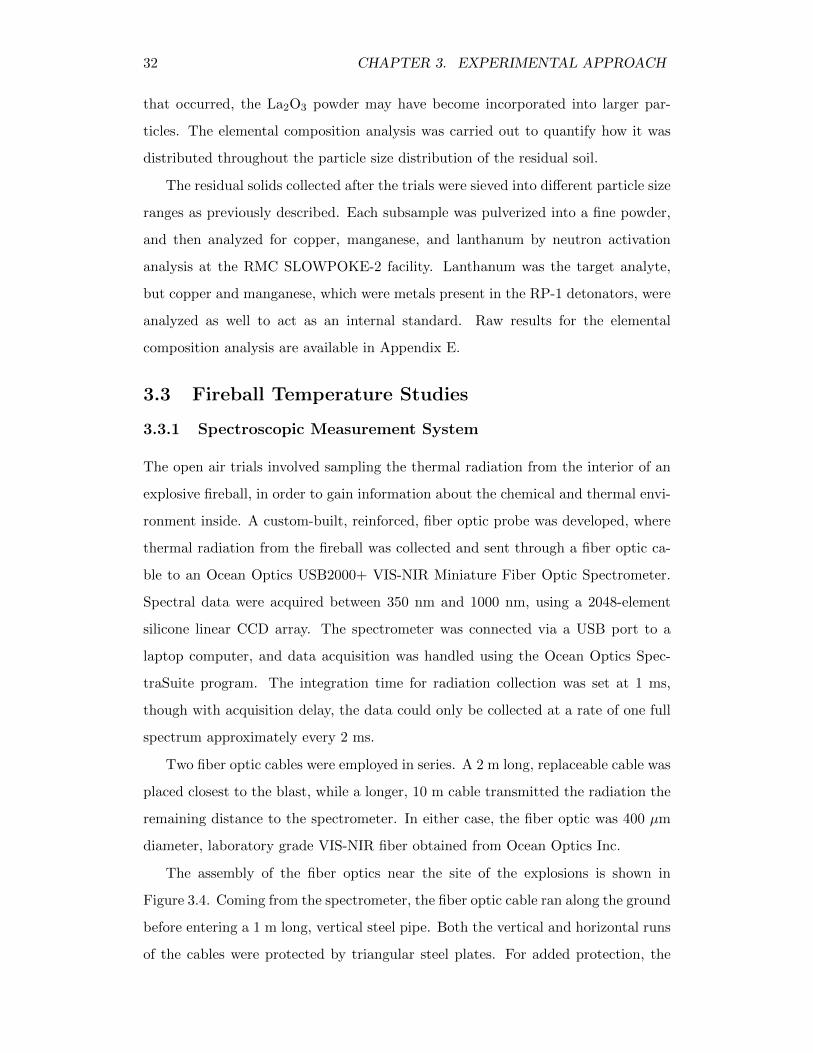
32 CHAPTER 3. EXPERIMENTAL APPROACH
that occurred, the La2O3 powder may have become incorporated into larger par-
ticles. The elemental composition analysis was carried out to quantify how it was
distributed throughout the particle size distribution of the residual soil.
The residual solids collected after the trials were sieved into different particle size
ranges as previously described. Each subsample was pulverized into a fine powder,
and then analyzed for copper, manganese, and lanthanum by neutron activation
analysis at the RMC SLOWPOKE-2 facility. Lanthanum was the target analyte,
but copper and manganese, which were metals present in the RP-1 detonators, were
analyzed as well to act as an internal standard. Raw results for the elemental
composition analysis are available in Appendix E.
3.3 Fireball Temperature Studies
3.3.1 Spectroscopic Measurement System
The open air trials involved sampling the thermal radiation from the interior of an
explosive fireball, in order to gain information about the chemical and thermal envi-
ronment inside. A custom-built, reinforced, fiber optic probe was developed, where
thermal radiation from the fireball was collected and sent through a fiber optic ca-
ble to an Ocean Optics USB2000+ VIS-NIR Miniature Fiber Optic Spectrometer.
Spectral data were acquired between 350 nm and 1000 nm, using a 2048-element
silicone linear CCD array. The spectrometer was connected via a USB port to a
laptop computer, and data acquisition was handled using the Ocean Optics Spec-
traSuite program. The integration time for radiation collection was set at 1 ms,
though with acquisition delay, the data could only be collected at a rate of one full
spectrum approximately every 2 ms.
Two fiber optic cables were employed in series. A 2 m long, replaceable cable was
placed closest to the blast, while a longer, 10 m cable transmitted the radiation the
remaining distance to the spectrometer. In either case, the fiber optic was 400 µm
diameter, laboratory grade VIS-NIR fiber obtained from Ocean Optics Inc.
The assembly of the fiber optics near the site of the explosions is shown in
Figure 3.4. Coming from the spectrometer, the fiber optic cable ran along the ground
before entering a 1 m long, vertical steel pipe. Both the vertical and horizontal runs
of the cables were protected by triangular steel plates. For added protection, the
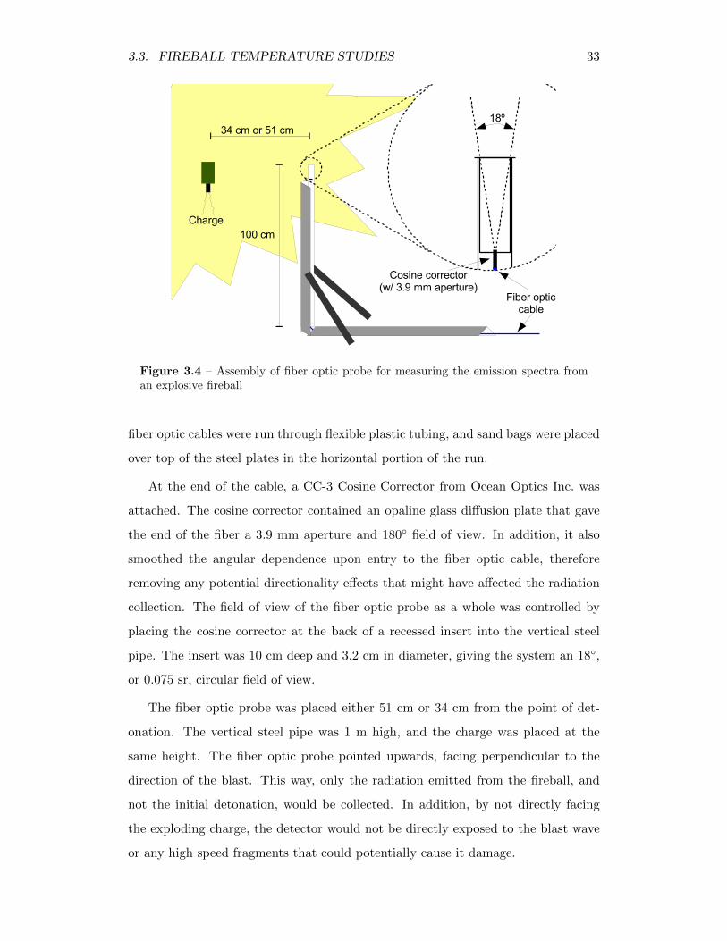
3.3. FIREBALL TEMPERATURE STUDIES 33
100 cm
34 cm or 51 cm
Charge
18º
Cosine corrector(w/ 3.9 mm aperture)
Fiber opticcable
Figure 3.4 – Assembly of fiber optic probe for measuring the emission spectra froman explosive fireball
fiber optic cables were run through flexible plastic tubing, and sand bags were placed
over top of the steel plates in the horizontal portion of the run.
At the end of the cable, a CC-3 Cosine Corrector from Ocean Optics Inc. was
attached. The cosine corrector contained an opaline glass diffusion plate that gave
the end of the fiber a 3.9 mm aperture and 180 field of view. In addition, it also
smoothed the angular dependence upon entry to the fiber optic cable, therefore
removing any potential directionality effects that might have affected the radiation
collection. The field of view of the fiber optic probe as a whole was controlled by
placing the cosine corrector at the back of a recessed insert into the vertical steel
pipe. The insert was 10 cm deep and 3.2 cm in diameter, giving the system an 18,
or 0.075 sr, circular field of view.
The fiber optic probe was placed either 51 cm or 34 cm from the point of det-
onation. The vertical steel pipe was 1 m high, and the charge was placed at the
same height. The fiber optic probe pointed upwards, facing perpendicular to the
direction of the blast. This way, only the radiation emitted from the fireball, and
not the initial detonation, would be collected. In addition, by not directly facing
the exploding charge, the detector would not be directly exposed to the blast wave
or any high speed fragments that could potentially cause it damage.
34 CHAPTER 3. EXPERIMENTAL APPROACH
3.3.2 Experimental Procedure
Five trials were carried out in total, and usable data were obtained over a duration of
about 20 ms, yielding 10 full spectra per trial (tabulated in Appendix F). The trials
involved detonating 175 g charges of Detasheet-C explosives, and were carried out
in the detonics bay at DRDC-Valcartier, a semi-enclosed space that allows energetic
materials to be set off in close proximity to instrumentation, while still offering the
required degree of protection to personnel and equipment.
The set-up of the fiber optic probe in the detonics bay is shown in Figure 3.5.
The bay is semi-circular, and is open to the outside on one side. The charges were
set off toward the inner most wall of the bay, near the fiber optic probe. The fiber
optic cable was run out from the bay, around, and back into the building through
one of the side walls. The spectrometer and associated equipment were inside the
building, separated from the blast by a protective concrete wall.
It should be noted, however, that a consequence of carrying out the explosions
in the detonics bay was that reflections of the blast wave off of the walls affected the
shape and position of the fireball. High speed video showed the fireball oscillating
in its shape and position as different reflections passed back through it, and these
would have in turn affected the relative position of the probe in the fireball.
Spectrometer &Instrumentation
High SpeedVideo
Detonics Bay
Charge Location
Probe Location
Fiber Optic
Figure 3.5 – Detonics bay
Chapter 4
Particle Breakup and GrowthMechanisms
In this section, the morphology of particles will be examined. Information about
the shape and structure of particles will be used to deduce how, when subjected to
an explosion, they can be broken up, how they can be consumed, and how they can
interact with one another.
Residual solids were collected after all the trials, and the material was separated
into several particle size ranges, using a mechanical sieve, and SEM micrographs
were taken of all the resulting particulate samples. These were compared to control
samples of soil that had not been exposed to a detonation. A substantial amount
of both qualitative and quantitative information has been obtained from this com-
prehensive set of micrographs. The ones shown in this section were selected to
specifically illustrate the different behaviours that are present, and are shown to
qualitatively surmise the main mechanisms that influence particle size.
4.1 Particle Combustion
When either C-4 or detasheet are detonated, because they are both underoxidized
explosives with a sufficiently negative oxygen balance, they produce carbonaceous
soot as a detonation product. When the soot is exposed to atmospheric oxygen, it
combusts as part of the fireball. Figure 4.1 shows a comparison of the residual soot
and ash that are generated during the closed vessel tests (without any soil present),
comparing explosions with an inhibited (po2∼= 0 kPa) and uninhibited secondary
combustion phase.
35
36 CHAPTER 4. PARTICLE BREAKUP AND GROWTH MECHANISMS
(a) shot C40629, po2 = 4 kPa
(b) shot C40810, po2 = 137 kPa
Figure 4.1 – SEM micrographs of explosive residue for shots carried out (a) in theabsence of oxygen and (b) in the presence of oxygen
4.2. MECHANICAL MECHANISMS 37
Figure 4.1a shows material collected from a shot that was carried out under a
low-oxygen atmosphere. Submicron-sized primary particles of carbonaceous soot
are held together in loose clusters, and give the material its light and fluffy texture.
The particulates seen in Figure 4.1b are more compact, and have a different texture.
Residual material here is from a detonation carried out with an initial oxygen partial
pressure of 137 kPa, where most of the carbonaceous soot has been consumed in the
afterburn reactions, leaving only ash and other incombustible solids behind.
It is not, however, only carbonaceous soot that can undergo particle combustion.
Black earth, which is a soil composed of organic matter, can also undergo combustion
when it becomes entrained in the fireball. When comparing the control black earth,
black earth collected after shots done in low-oxygen, and black earth collected after
shots done in an oxygenated atmosphere (Figure 4.2), there is a distinct reduction
in the number of the smallest particles. Combustion erodes the surfaces of the black
earth particles, and particles that are below a certain critical diameter completely
disappear.
Note, however, that with this single exception, where the smallest particles are
consumed in the fireball, there is little other change in the shape and structure of
black earth particles from one sample to another. As will be discussed in Chapter 6,
this is actually an important consideration, because black earth does not undergo
agglomeration in the fireball like the other types of soil, such as clay, coarse sand,
and fine sand, all do.
4.2 Mechanical Mechanisms
Fracturing is a mechanical effect that occurs when the shock breaks the particles
of hard, singularly-grained materials (e.g., quartz sand) apart. This is shown in
the < 47 µm fraction of particles of detonation-exposed sand, where the small and
highly angular fragments of fractured particles that are generated can be seen, as
in Figures 4.3b and 4.3c. The fresh fine sand in Figure 4.3a, on the other hand, is
composed of fairly uniform, polyhedral grains, the majority of which (by volume)
are relatively large, with few being less in diameter than about 40 µm.
Particle fracturing was only observed with the two types of sand, however. In
other soil types, like black earth and clay (Figures 4.2 and 4.5, respectively) particles
38 CHAPTER 4. PARTICLE BREAKUP AND GROWTH MECHANISMS
(a) black earth (< 47 µm range), control
(b) shot DS0923 (< 47 µm range), po2 = 4 kPa
(c) shot DS1214 (< 47 µm range), po2 = 205 kPa
Figure 4.2 – SEM micrographs of black earth, comparing (a) the control black earthto residual solids collected after shots carried out (b) in the absence of oxygen and (c)in the presence of oxygen
4.2. MECHANICAL MECHANISMS 39
(a) fine sand (< 47 µm range), control
(b) shot C40914 (< 47 µm range), po2 = 4 kPa
(c) shot DS1104 (< 47 µm range), po2 = 91 kPa
Figure 4.3 – SEM micrographs of fracturing, comparing (a) the control fine sand tofine sand collected after shots carried out (b) in the absence of oxygen and (c) in thepresence of oxygen
40 CHAPTER 4. PARTICLE BREAKUP AND GROWTH MECHANISMS
are loose clusters of smaller primary particles. Their strength would be minimal,
there would be a lot of void space, and there would be little or no resistance to
deformation. When the bed of black earth or clay is subjected to the blast wave from
an explosion, part of it compacts down into a dense matrix (although compaction
effects were observed directly while removing residual solids from vessel, rather than
from SEM). Sand, on the other hand, is not compacted by the force of the blast, and
so individual particles are subject to greater forces that break them apart. Therefore,
the same forces that make the ‘stronger’ particles more susceptible to being broken
up cause the ‘weaker’ particles to flow past one another, deform, and squeeze out
their void space. Instead of being broken up, clay or black earth particles compress
together.
4.3 Particle Interactions
Fracturing and compaction are mechanical effects caused by the force of the blast.
After the initial detonation, however, particles can interact with one another to
produce agglomerates. Figure 4.4 shows coarse sand particulates collected in the
250-297 µm range. The control coarse sand particles in Figure 4.4a have the same
polyhedral grain shapes as those in Figure 4.3a, only larger.
The deposition of small soot and ash particulates onto larger grains occurs re-
gardless of whether or not the trials were carried out in the presence of oxygen. This
can be seen in Figures 4.4b and 4.4c as a light coating on the surface of particles.
When sand particles are exposed to higher temperatures for longer times, how-
ever, they can interact with one another to form agglomerates. These are seen in
Figure 4.4c: irregularly shaped agglomerates made up of smaller sand particulates
that have fused together in the high heat of the fireball.
When the clay in Figure 4.5a and Figure 4.5b are compared, it can be seen
that, except for the addition of some soot and ash, there is not much difference
between the control clay, and clay collected after a shot done in low-oxygen. As
previously discussed, this is because clay does not undergo fracturing, and there is
no other mechanism to this point that affects the size or shape of particles. However,
when shots with clay are carried out in the presence of oxygen, the formation of
agglomerates that are orders of magnitude larger than particles in the original clay
4.3. PARTICLE INTERACTIONS 41
(a) coarse sand (250-297 µm range), control
(b) shot C40830 (250-297 µm range), po2 = 4 kPa
(c) shot C40907 (250-297 µm range), po2 = 138 kPa
Figure 4.4 – SEM micrographs of agglomeration, comparing (a) the control coarsesand to coarse sand collected after shots carried out (b) in the absence of oxygen and(c) in the presence of oxygen
42 CHAPTER 4. PARTICLE BREAKUP AND GROWTH MECHANISMS
(a) clay (no sieve processing), control
(b) shot C40218 (250-297 µm range), po2 = 4 kPa
(c) shot DS1007 (600-841 µm range), po2 = 138 kPa
Figure 4.5 – SEM micrographs of agglomeration, comparing (a) the control clay toresidual solids collected after shots carried out (b) in the absence of oxygen and (c) inthe presence of oxygen
4.4. SUMMARY 43
can be observed. Figure 4.5c shows a sample in the 600-841 µm range from a
shot that was carried out with an initial oxygen partial pressure of 138 kPa. The
clay particles fuse together during the secondary combustion phase, and form the
enormous, porous structures seen in the micrograph.
For black earth, agglomeration does not occur as it requires that particles fuse
together after they collide. The sand and clay particles can sinter together as they
are effectively baked in the high heat of the fireball. However, because the black
earth particles are burning and their surfaces are being continually eroded away in
the fireball, they cannot stay fused together. The combustion of a particle, as it has
been seen, therefore inhibits its agglomeration.
4.4 Summary
In summary, the particle breakup and growth mechanisms that have been observed
to occur include fracturing and compaction (from the initial blast), as well as particle
combustion and agglomeration (in the secondary fireball). Fracturing occurs in
harder, granular soils like sand, and occurs when the force of the blast breaks apart
individual grains, but is not observed in soils like clay and black earth, in which
individual particles are made up of smaller primary particles; compaction of these
loose soils into a hard matrix is observed instead.
Fracturing and compaction are mechanical effects caused by the force of the
blast, and occur whether or not the shots are carried out in the presence of oxygen.
Agglomeration, however, is only observed when particles are allowed to fuse together
in the high heat of the fireball, as has been seen with sand and clay.
Particle combustion also occurs when shots are carried out in the presence of
oxygen. Carbonaceous soot is consumed in the secondary fireball, as is black earth.
In fact, the lack of any agglomeration of black earth particles is probably precisely
because combustion at the surface of those particles inhibits them from fusing to-
gether.

44 CHAPTER 4. PARTICLE BREAKUP AND GROWTH MECHANISMS
Chapter 5
Explosion Thermochemistry
In this chapter, the thermochemistry of the fireball will be described. The energy
that is released from the fireball is a key factor, and drives many of the particle
dynamics: it provides the sustained, high temperature, and turbulent environment
that allows different soot and ash, target, and entrained soil particulates to interact,
deposit on surfaces, and agglomerate with one another. When the entrained soil is
combustible, as in the case for black earth, though, it can add to the combustion
energy and enhance the size and duration of the fireball. There is, therefore, a two-
way relationship between fireball energy and the particle dynamics, and so being
able to describe how that energy is liberated is important.
5.1 Thermochemical Model of an Explosion
5.1.1 General Description
There are two distinct and sequential events that occur in an explosion. The first,
detonation, is where the explosives undergo a shock-induced chemical reaction. The
material is (mostly) converted into gaseous detonation products, which under ex-
tremely high pressures initially, expand outwards. The fireball occurs during this
second phase, when underoxidized detonation products mix with surrounding air.
Detonation is basically a self-contained combustion process, where the detonation
wave initiates a self-oxidation reaction to produce high energy, high pressure deto-
nation products. This conversion happens very quickly, over less than a microsec-
ond, and is confined to millimeter sections of the detonating explosive compound
(Cooper, 1996). After the detonation wave passes, though, the highly condensed
product gases, free from any barrier, expand outward.
45
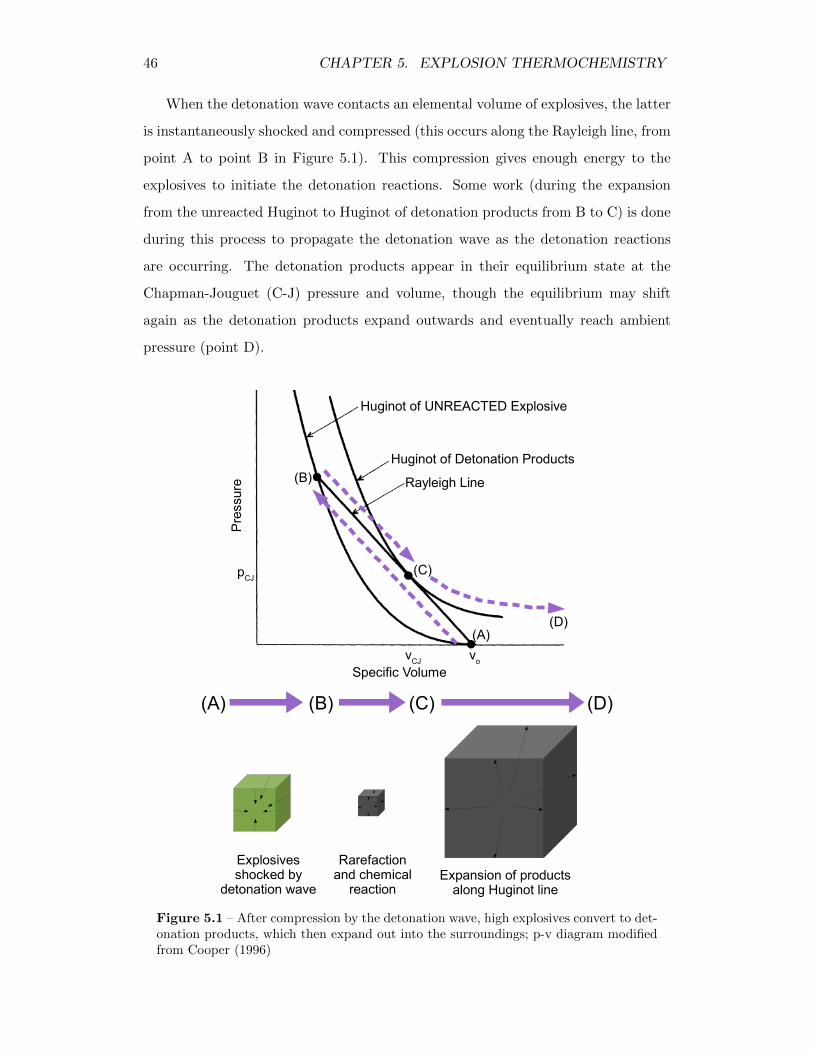
46 CHAPTER 5. EXPLOSION THERMOCHEMISTRY
When the detonation wave contacts an elemental volume of explosives, the latter
is instantaneously shocked and compressed (this occurs along the Rayleigh line, from
point A to point B in Figure 5.1). This compression gives enough energy to the
explosives to initiate the detonation reactions. Some work (during the expansion
from the unreacted Huginot to Huginot of detonation products from B to C) is done
during this process to propagate the detonation wave as the detonation reactions
are occurring. The detonation products appear in their equilibrium state at the
Chapman-Jouguet (C-J) pressure and volume, though the equilibrium may shift
again as the detonation products expand outwards and eventually reach ambient
pressure (point D).
(A) (B) (C) (D)
Explosivesshocked by
detonation wave
Rarefactionand chemical
reactionExpansion of products
along Huginot line
Specific Volume
Pre
ssur
e
Huginot of UNREACTED Explosive
Huginot of Detonation Products
Rayleigh Line
(A)
(B)
(C)
(D)
vCJ
pCJ
vo
Figure 5.1 – After compression by the detonation wave, high explosives convert to det-onation products, which then expand out into the surroundings; p-v diagram modifiedfrom Cooper (1996)
5.1. THERMOCHEMICAL MODEL OF AN EXPLOSION 47
A very large number of species can be produced from a detonation. For CHNO
explosives, major components are typically CO2, H2O, and N2, but depending on
the oxygen balance in the explosive, carbonaceous soot, along with CO, H2, CH4,
NH3, and numerous other trace gases, can also be formed. The proportion of each
compound is a function of the oxygen balance of the explosive, which defines how
‘rich’ or ‘lean’ it is in terms of its potential for self-oxidation.
It is generally assumed that detonation products are in equilibrium when they
appear at the C-J state, given the high initial temperatures and pressures. In fact,
as the detonation products expand and cool, the product composition will continue
to shift according to the local equilibrium conditions until they are cool enough that
kinetic barriers start to take effect, reactions slow.
In the absence of anything else, the product composition will be fixed below
a certain temperature. But in reality, since products will start to mix with the
surrounding air, many of them can start to undergo further combustion. The main
components, like CO2 and H2O, are fully oxidized, while most others are not. They
can react further, liberating more energy. Depending on the oxygen balance of the
explosives, the energy released from this secondary fireball can even be greater than
that released in the initial detonation.
5.1.2 Thermochemical Prediction Using CHEETAH Code
The starting materials, or fuel, for the secondary combustion reactions are the un-
deroxidized detonation products. To predict the composition of these, as well as
other detonation properties, the thermochemical solver, CHEETAH, developed at
Lawrence Livermoore National Laboratory (Fried and Souers, 1994), was used. The
code is an advanced thermodynamic equilibrium solver based on the BKWC equa-
tion of state (C for CHEETAH), a modified version of the semi-empirical BKW
equation of state (Cowan and Fickett, 1956), but improved to match to a long pro-
gram of cylinder tests, and optimized to describe high pressure, energetic systems
(Fried and Souers, 1994).
CHEETAH was employed to obtain, among other things, predictions of the heats
of detonation, and of the product compositions. Simulations were run using a copy
of CHEETAH at DRDC Valcartier, and the thermochemical properties that were
48 CHAPTER 5. EXPLOSION THERMOCHEMISTRY
Table 5.1 – Thermochemical parameters of C-4 explosive (Fried and Souers, 1994;Cooper, 1996; Liley et al., 1997)
(a) properties of the components in the initial explosive composition
Component Chemical FormulaMass
Fraction
MolecularWeight/ g·mol−1
MoleFraction
Heat ofFormation/ kJ·mol−1
RDX C3H6N6O6 0.910 222.13 0.869 +69polyisobutylene (C4H8)n 0.021 56.10 0.080 −88
fuel oil ∼ C10H16 0.016 136.43 0.025 +29DEH sebacate C26H50O4 0.053 426.66 0.026 −1335
total C3.86H7.57N5.22O5.32 1.000 212.20 1.000 +19
oxygen balance: −46.6%
(b) conditions at the Chapman-Jouguet state, as cal-culated by CHEETAH
Parameter Value
shock velocity 8.03 km·s−1
C-J pressure 24.69 GPaC-J density 2.094 g·cm−3
C-J volume 101 cm3·mol−1
C-J temperature 3762 Kequilibrium freeze-out temperature 2145 K
(c) product compositions at C-J state and freeze-out temperature, as calculated by CHEETAH
Condition CO2 H2O N2 CO H2 CH4 NH3 other C(s)
/ mol(product)·mol(explosive)−1
C-J state 1.63 1.33 2.42 0.03 0.09 0.31 0.37 0.64 1.01freeze-out 1.38 1.92 2.55 0.62 0.59 0.52 0.12 0.03 1.29
(d) heats of reaction and oxygen stoichiometry for different stages of the explosion, usingfreeze-out equilibrium composition
Reaction Oxygen Stoichiometry Heat of Reaction/ mol(O2)·mol(explosive)−1 / kJ·mol−1 / kJ·g−1
total combustion 3.09 −2620 −12.35detonation – −1144 −5.39afterburn 3.09 −1476 −6.96
– for gas phase material 1.80 −967 −4.56– for carbonaceous soot 1.29 −509 −2.40
5.1. THERMOCHEMICAL MODEL OF AN EXPLOSION 49
Table 5.2 – Thermochemical parameters of detasheet explosive (Fried and Souers,1994; Cooper, 1996; Liley et al., 1997)
(a) properties of the components in the initial explosive composition
Component Chemical FormulaMass
Fraction
MolecularWeight/ g·mol−1
MoleFraction
Heat ofFormation/ kJ·mol−1
PETN C5H8N8O12 0.630 316.15 0.663 −527NC (12.6% N) (C6H7.55N2.45O9.90)n 0.080 272.39 0.098 −708
ATBC C20H34O8 0.290 402.47 0.239 −1820
total C8.69H14.19N2.89O10.84 1.000 332.56 1.000 −855
oxygen balance: −65.6%
(b) conditions at the Chapman-Jouguet state duringdetonation, as calculated by CHEETAH
Parameter Value
shock velocity 7.09 km·s−1
C-J pressure 17.93 GPaC-J density 1.943 g·cm−3
C-J volume 166 cm3·mol−1
C-J temperature 3099 Kequilibrium freeze-out temperature 2145 K
(c) product compositions at C-J state and freeze-out temperature, as calculated by CHEETAH
Condition CO2 H2O N2 CO H2 CH4 NH3 other C(s)
/ mol(product)·mol(explosive)−1
C-J state 3.39 3.00 1.26 0.05 0.15 0.72 0.36 1.00 3.09freeze-out 3.09 4.06 1.37 0.58 0.69 0.96 0.15 0.09 3.96
(d) heats of reaction and oxygen stoichiometry for different stages of the explosion, usingfreeze-out equilibrium composition
Reaction Oxygen Stoichiometry Heat of Reaction/ mol(O2)·mol(explosive)−1 / kJ·mol−1 / kJ·g−1
total combustion 6.82 −4595 −13.82detonation – −1493 −4.49afterburn 6.82 −3102 −9.33
– for gas phase material 2.86 −1543 −4.64– for carbonaceous soot 3.96 −1559 −4.69
50 CHAPTER 5. EXPLOSION THERMOCHEMISTRY
obtained are given in Tables 5.1 and 5.2. The code predicted heats of detonation
of 5.4 kJ·g−1 and 4.5 kJ·g−1 for C-4 and detasheet, respectively. Measurements of
the heats of detonation with the calorimeter put these values at 5.1±0.2 kJ·g−1 and
4.5±0.2 kJ·g−1, which compare quite well.
Part (a) of Table 5.1 and Table 5.2 give the composition of the explosives, in
terms of both their explosive ingredients as well as any fillers or additives. These
values essentially represent the input to the CHEETAH code. Part (b) gives the
different parameters, like the pressure and density, calculated at the Chapman-
Jouguet condition, as well as the calculated shock velocity and the temperature
at which the detonation product equilibrium is assumed to freeze-out. At a certain
point, kinetic barriers start to slow the equilibrium reaction, and CHEETAH handles
this by assuming that components are in perfect equilibrium until and abrupt point,
the freeze-out temperature, below which no more reactions occur. Part (c) gives
an abbreviated list of detonation products and their relative compositions at both
the C-J state, as well as at the final freeze-out condition. The most important
components out of the 63 considered by CHEETAH are given. Finally, part (d)
gives the heat of combustion, heat of detonation, and heat of afterburn for the
explosives. The heat of afterburn, specifically, is also divided into the component
from the condensed phase detonation products (i.e. carbonaceous soot), and that
from the gas phase detonation products.1
5.1.3 Thermochemical Model of Secondary Combustion
A large number of detonation products can be produced during the initial detonation
phase of an explosion, and many of those will react with the oxygen in the air as
they expand outward. The thermodynamic end state to which the reacting species
work toward is dictated by the equilibrium conditions involved. An argument that
will be made in this chapter, however, is that the transport of species is the rate
limiting step, and that certain species can react with oxygen more efficiently and
achieve that thermodynamic end state before others.
Ultimately, carbonaceous soot would react with oxygen to produce carbon diox-
ide. However, carbon monoxide would be an intermediate in that reaction, and on
1These are all given in terms of complete combustion to CO2, H2O, etc., as opposed to partialcombustion to CO or other partly oxidized species
5.1. THERMOCHEMICAL MODEL OF AN EXPLOSION 51
the microscale interfaces between soot particulates and air, one would expect the
carbon monoxide to be initially evolved after the oxygen reacts with the carbon.
C(s) + 12O2 → CO (5.1)
The carbon monoxide produced here, along with the CO, H2, CH4, NH3, and all
the other underoxidized detonation products, can all undergo further combustion
when they come into contact with atmospheric oxygen.
CO + 12O2 → CO2
H2 + 12O2 → H2O
CH4 + 2O2 → CO2 + 2H2O
NH3 + 34O2 → 1
2N2 + 32H2O
(5.2)
These reactions are all in competition with one another, and proceed at different
rates depending on both the transport mechanisms and kinetics. Even if similar
compounds react at similar rates are classed together, there are at least two classes
of detonation products that react through fundamentally different mechanisms.
Gas phase products react homogeneously as gases, requiring pockets of gas to
mix together, and for reacting species to meet at the molecular level. There are
many different gaseous detonation products that are combustible, from light chain
hydrocarbons and CO, to hydrogen and simple nitrogen compounds. All of the
different gas phase detonation products can be taken together, and can be considered
as an ‘average’ CHNO gas:
CxHyNwOz + νo2,gO2 → xCO2 + y2H2O + w
2 N2 (5.3)
where νo2,g is the stoichiometric coefficient for oxygen for the gas phase reactions.
Condensed phase products, like carbonaceous soot, react heterogeneously, requir-
ing oxygen to diffuse toward their surface, react, and for the (partial) combustion
products to diffuse away. CHEETAH assumes that carbon is the only condensed
phase species produced during the detonation, but because other materials, like the
gun tape was used to wrap the charges, were also used, the condensed phase material
can be assumed to react together with a more general, ‘average’ chemical formula:
52 CHAPTER 5. EXPLOSION THERMOCHEMISTRY
CxHyNwOz,(s) + νo2,cO2 → xCO2 + y2H2O + w
2 N2 (5.4)
where νo2,c is the stoichiometric coefficient for oxygen for condensed phase reactions.
It is assumed in this work that all reaction products can be lumped into these
two classes, and that all individual compounds within a class react at the same rate.
After all, for reactions that are transport-limited (as opposed to kinetically limited),
the physical processes of mixing and getting the reacting species to come into con-
tact with one another is the rate limiting step. Small kinetic differences between
individual species would be much less important, since the chemical reactions that
occur in a flame are typically much faster than the physical diffusion processes of
the reacting species, as well as the transport of the heat that is generated (Turns,
2006; Dixon-Lewis, 1968). This is especially true in an explosive fireball due to the
physical separation between the detonation products and the air. Major differences
would likely be seen between species that mix in fundamentally different ways, as
with gas-gas versus gas-particle reactions. As a result, the differences in the rates
at which individual solid or individual gas species react are likely negligible.
Consider the case where gas phase species are reacting in the fireball at a rate
rg, and condensed phase species are reacting at rc. Or more precisely for rg and
rc, consider the rates at which oxygen is consumed by the respective reactions. The
fractional rate, f , at which oxygen is consumed in the gas reactions relative to the
total rate at which oxygen is being consumed, can therefore be defined as:
f ≡ rgrc + rg
(5.5)
If a volume contains both detonation products and air, then the rate that the
detonation products are consumed will be directly related to the rate of oxygen
consumption by:
dng = f · 1
νo2,gdno2 (5.6a)
dnc = (1− f) · 1
νo2,cdno2 (5.6b)
where ng is moles of the gas phase reactants, nc is moles of condensed phase reac-
tants, and no2 is moles of oxygen.
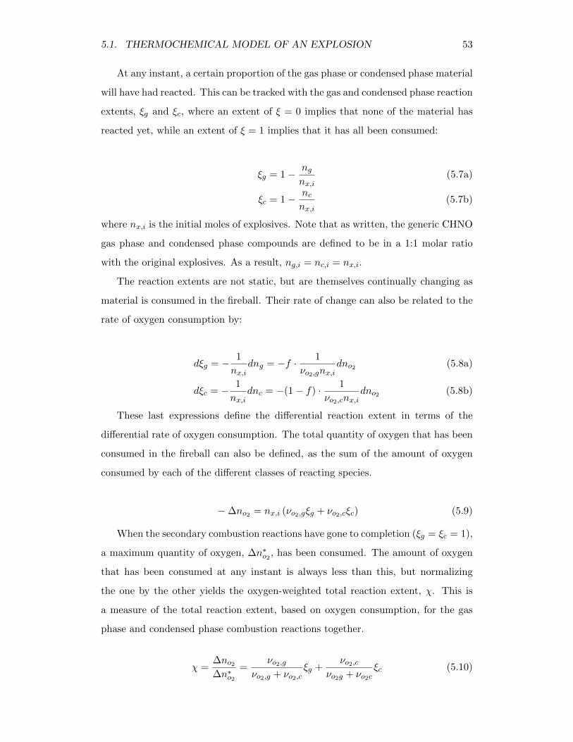
5.1. THERMOCHEMICAL MODEL OF AN EXPLOSION 53
At any instant, a certain proportion of the gas phase or condensed phase material
will have had reacted. This can be tracked with the gas and condensed phase reaction
extents, ξg and ξc, where an extent of ξ = 0 implies that none of the material has
reacted yet, while an extent of ξ = 1 implies that it has all been consumed:
ξg = 1− ngnx,i
(5.7a)
ξc = 1− ncnx,i
(5.7b)
where nx,i is the initial moles of explosives. Note that as written, the generic CHNO
gas phase and condensed phase compounds are defined to be in a 1:1 molar ratio
with the original explosives. As a result, ng,i = nc,i = nx,i.
The reaction extents are not static, but are themselves continually changing as
material is consumed in the fireball. Their rate of change can also be related to the
rate of oxygen consumption by:
dξg = − 1
nx,idng = −f · 1
νo2,gnx,idno2 (5.8a)
dξc = − 1
nx,idnc = −(1− f) · 1
νo2,cnx,idno2 (5.8b)
These last expressions define the differential reaction extent in terms of the
differential rate of oxygen consumption. The total quantity of oxygen that has been
consumed in the fireball can also be defined, as the sum of the amount of oxygen
consumed by each of the different classes of reacting species.
−∆no2 = nx,i (νo2,gξg + νo2,cξc) (5.9)
When the secondary combustion reactions have gone to completion (ξg = ξc = 1),
a maximum quantity of oxygen, ∆n∗o2 , has been consumed. The amount of oxygen
that has been consumed at any instant is always less than this, but normalizing
the one by the other yields the oxygen-weighted total reaction extent, χ. This is
a measure of the total reaction extent, based on oxygen consumption, for the gas
phase and condensed phase combustion reactions together.
χ =∆no2∆n∗o2
=νo2,g
νo2,g + νo2,cξg +
νo2,cνo2g + νo2c
ξc (5.10)
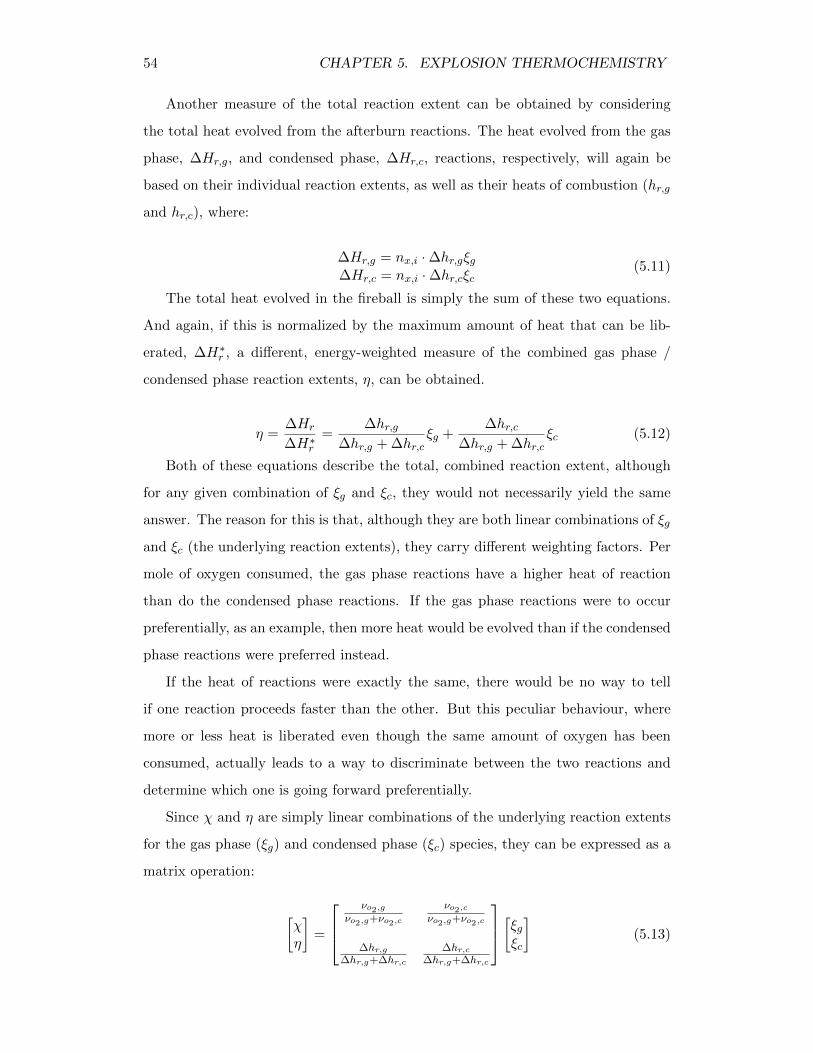
54 CHAPTER 5. EXPLOSION THERMOCHEMISTRY
Another measure of the total reaction extent can be obtained by considering
the total heat evolved from the afterburn reactions. The heat evolved from the gas
phase, ∆Hr,g, and condensed phase, ∆Hr,c, reactions, respectively, will again be
based on their individual reaction extents, as well as their heats of combustion (hr,g
and hr,c), where:
∆Hr,g = nx,i ·∆hr,gξg∆Hr,c = nx,i ·∆hr,cξc
(5.11)
The total heat evolved in the fireball is simply the sum of these two equations.
And again, if this is normalized by the maximum amount of heat that can be lib-
erated, ∆H∗r , a different, energy-weighted measure of the combined gas phase /
condensed phase reaction extents, η, can be obtained.
η =∆Hr
∆H∗r=
∆hr,g∆hr,g + ∆hr,c
ξg +∆hr,c
∆hr,g + ∆hr,cξc (5.12)
Both of these equations describe the total, combined reaction extent, although
for any given combination of ξg and ξc, they would not necessarily yield the same
answer. The reason for this is that, although they are both linear combinations of ξg
and ξc (the underlying reaction extents), they carry different weighting factors. Per
mole of oxygen consumed, the gas phase reactions have a higher heat of reaction
than do the condensed phase reactions. If the gas phase reactions were to occur
preferentially, as an example, then more heat would be evolved than if the condensed
phase reactions were preferred instead.
If the heat of reactions were exactly the same, there would be no way to tell
if one reaction proceeds faster than the other. But this peculiar behaviour, where
more or less heat is liberated even though the same amount of oxygen has been
consumed, actually leads to a way to discriminate between the two reactions and
determine which one is going forward preferentially.
Since χ and η are simply linear combinations of the underlying reaction extents
for the gas phase (ξg) and condensed phase (ξc) species, they can be expressed as a
matrix operation:
[χη
]=
νo2,g
νo2,g+νo2,c
νo2,cνo2,g+νo2,c
∆hr,g∆hr,g+∆hr,c
∆hr,c∆hr,g+∆hr,c
[ξgξc
](5.13)
5.1. THERMOCHEMICAL MODEL OF AN EXPLOSION 55
The reaction extents can then be computed from χ and η simply by taking the
matrix inverse:
[ξgξc
]=
1∆hr,gνo2,g
− ∆hr,cνo2,c
−νo2,g+νo2,c
νo2,g· ∆hr,cνo2,c
∆hr,g+∆hr,c∆hr,g
· ∆hr,gνo2,g
νo2,g+νo2,cνo2,c
· ∆hr,gνo2,g
−∆hr,g+∆hr,c∆hr,g
· ∆hr,cνo2,c
[χη
](5.14)
Thus the underlying reaction extents can be found directly as long as η and χ
are both known. For this inversion to be possible, however, the heats of reaction per
mole of oxygen consumed must be different. If they are the same, the determinant
in Equation 5.14 would be zero, and the matrix in Equation 5.13 would be singular.
Even if the two are close, the large magnitudes of elements in the inverse matrix
would mean that any errors with η or χ would be greatly magnified. As long as the
differences in heat of reaction are large enough, though, this gives a powerful tool
that allows the underlying reaction extents to be determined.
In addition to the underlying extents, the fractional reaction rate, f , can also
be determined. The differential rate at which heat is evolved in the fireball can be
obtained using Equation 5.12 to yield:
dη =∆hr,g
∆hr,g + ∆hr,cdξg +
∆hr,c∆hr,g + ∆hr,c
dξc (5.15)
Relating this expression to the rate of oxygen consumption, using Equation 5.8,
yields:
dη =1
nx,i
[∆hr,g
νo2,g(∆hr,g + ∆hr,c)· f +
∆hr,cνo2,c(∆hr,g + ∆hr,c)
· (1− f)
]dno2 (5.16)
As χ is the ratio of the amount of oxygen that has been consumed in the fireball,
to the total amount that stoichiometrically could be consumed (Equation 5.10), then
the rate at which χ changes can also be related to the rate of oxygen consumption
by:
dχ =1
nx,i· 1
νo2,g + νo2,cdno2 (5.17)
These last two expressions can be combined to obtain the following equation,
which expresses the derivative of η with respect to χ in terms of f :
56 CHAPTER 5. EXPLOSION THERMOCHEMISTRY
dη
dχ=
νo2,g + νo2,c∆hr,g + ∆hr,c
· ∆hr,gνo2,g
· f +νo2,g + νo2,c
∆hr,g + ∆hr,c· ∆hr,cνo2,c
· (1− f) (5.18)
Data from the calorimetry experiments can be transformed so that they can
be expressed in terms of the energy-weighted and oxygen weighted total reaction
extents. From a plot of η versus χ, the slope at any point is related to the fractional
rate, f , at which oxygen is consumed in the gas phase reaction. Since the gas phase
reactions release more energy per mole of oxygen consumed than the condensed
phase reactions, a higher value for the slope means that the gas phase reactions are
going forward preferentially, while a lower value means that the condensed phase
reactions are preferred.
5.2 Calorimetry Results
Calorimetry results are available for 50 closed vessel trials in total. In addition, cali-
brations were carried out in order to relate the actual measurements of temperature
rise to heat output. In addition, since the gun tape that holds the charge together
and black earth soil were also combustible, separate calorimetry experiments were
carried out to determine their contribution toward the total observed temperature
rise.
5.2.1 Calibration of the Detonation Calorimeter
The calibration trials that have been carried out have employed between 1 g and 5 g
of benzoic acid and are plotted in Figure 5.2. A one parameter linear regression was
carried out on the calibration points, fitting an equation of the form Qcorr = βcal∆T .
The estimated slope was found to be βcal = 94±1 kJ·C−1. The standard error, sβ,
correlation coefficient, R2, Student’s t-test statistic, t = β/sβ, and the probability,
P , that the parameter is not significantly different from zero, are also included in
Figure 5.2.
5.2.2 Calorimetry of Auxiliary Material
A separate calorimetric study was conducted of gun tape and black earth, since
neither have reliable literature values for their heats of combustion. Tests were
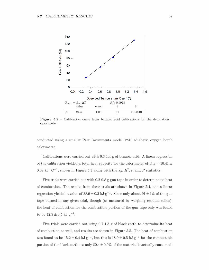
5.2. CALORIMETRY RESULTS 57
Qcorr = βcal∆T R2: 0.9978value error t P
β 94.40 1.03 91 < 0.0001
Figure 5.2 – Calibration curve from benzoic acid calibrations for the detonationcalorimeter
conducted using a smaller Parr Instruments model 1241 adiabatic oxygen bomb
calorimeter.
Calibrations were carried out with 0.3-1.4 g of benzoic acid. A linear regression
of the calibration yielded a total heat capacity for the calorimeter of βcal = 10.41±
0.08 kJ·C−1, shown in Figure 5.3 along with the sβ, R2, t, and P statistics.
Five trials were carried out with 0.2-0.8 g gun tape in order to determine its heat
of combustion. The results from these trials are shown in Figure 5.4, and a linear
regression yielded a value of 38.9± 0.2 kJ·g−1. Since only about 91± 1% of the gun
tape burned in any given trial, though (as measured by weighing residual solids),
the heat of combustion for the combustible portion of the gun tape only was found
to be 42.5± 0.5 kJ·g−1.
Five trials were carried out using 0.7-1.3 g of black earth to determine its heat
of combustion as well, and results are shown in Figure 5.5. The heat of combustion
was found to be 15.2± 0.4 kJ·g−1, but this is 18.9± 0.5 kJ·g−1 for the combustible
portion of the black earth, as only 80.4± 0.9% of the material is actually consumed.
58 CHAPTER 5. EXPLOSION THERMOCHEMISTRY
Q = βcal∆T R2: 0.9976value error t P
β 10.408 0.082 127 < 0.0001
Figure 5.3 – Calibration curve from benzoic acid calibrations for the Parr Instrumentsmodel 1241 adiabatic oxygen bomb calorimeter
Q = β ·mgt R2: 0.9993value error t P
β 38.95 0.38 103 < 0.0001
Figure 5.4 – Trials to determine gun tape heat of combustion
5.2. CALORIMETRY RESULTS 59
Q = β ·mbe R2: 0.9481value error t P
β 15.20 0.39 39 < 0.0001
Figure 5.5 – Trials to determine black earth heat of combustion
5.2.3 Calorimetry Measurements
Figure 5.6 shows the detonation calorimeter measurements for the total heat release
from the C-4 and detasheet shots as a function of the initial partial pressure of
oxygen in the detonation vessel. The data are from all 50 successful trials, and
include those carried out with explosives alone, with one of the four different types
of soil (coarse sand, fine sand, black earth, clay), and with the La2O3 tracer. The
results presented in the figure have been corrected so that the heat contribution from
the RP-83 detonator, measured as 8 ± 2 kJ, have been removed. The actual heat
measurements were reduced by this value to give the values presented in Figure 5.6.
An upward trend is observed in the data where the amount of liberated heat
increased directly with the amount of available oxygen. When trials were carried
out in low-oxygen, independent of whatever soil was present, data points were fairly
tightly grouped. The heat of detonation was measured as 5.1±0.2 kJ·g−1 for C-4 and
as 4.5± 0.2 kJ·g−1 for detasheet. These values compare very well to the 5.4 kJ·g−1
and 4.5 kJ·g−1 that were respectively predicted for C-4 and detasheet with the
CHEETAH code (Tables 5.1 and 5.2).
60 CHAPTER 5. EXPLOSION THERMOCHEMISTRY
Figure 5.6 – Energy release from explosives as a function of the initial oxygen partialpressure
The addition of oxygen to the vessel allowed the secondary combustion of the
detonation products to proceed, thereby allowing more energy to be liberated. How-
ever, this did not proceed at a universal rate. For example, since the detasheet had
a lower oxygen balance than the C-4, a higher proportion of its total combustion
energy was released during the afterburn phase and less during the initial detonation
phase. In fact, detasheet was capable of releasing more energy than C-4 when pre-
sented with enough oxygen, as evidenced by the maximum measured heat releases
in Figure 5.6.
Although most of the soil types would not have participated in the secondary
combustion reactions, black earth did. The total heat released from several of the
trials can be seen below the general trend, and they correspond to the trials with
black earth. For the trials carried out at 140 kPa, afterburn reactions released
about 37% less energy for C-4, and 26% less energy for detasheet, as compared with
baseline trials and trials carried out with other types of soil.
5.3. DETONATION PRODUCT COMBUSTION 61
5.3 Detonation Product Combustion
The purpose of this section is to describe the application of the thermochemical
model to the calorimetry measurements that were presented in the last section, to
gain information about how the gas and condensed phase species react.
5.3.1 Computing χ and η from data
The first step is to take the measurements from the calorimetry experiments and
transform them into the oxygen-weighted and energy-weighted total reaction ex-
tents, χ and η.
The oxygen-weighted total reaction extent is the ratio of the number of moles of
oxygen in the detonation vessel (which can be computed from the measured initial
partial pressure), to the number of moles of fuel, weighted by how much oxygen is
required for complete combustion. It was not only the detonation products from the
explosives that participated in the secondary combustion reactions, however; the
tape used to hold the charge together and the polyethylene vials used in the lan-
thanum oxide tracer trials also took part. These auxiliary materials also underwent
combustion in the fireball, and thus also participated in the consumption of oxygen.
The oxygen-weighted total reaction extent, therefore, can be computed from
measured values by:
χ =no2,i
νo2,xnx,i + νo2,gtngt,i + νo2,penpe,i(5.19)
where νo2,x = νo2,g + νo2,c is the combined reaction coefficient for all the detonation
products, gas and condensed phases taken together, while νo2,gt and νo2,pe are the
reaction coefficients for the auxiliary materials, assuming a composition of C4H8 (i.e.
mostly polyisobutylene with polyethylene backing; cotton mesh, fillers, etc. ignored)
for the tape and C2H4 for the polyethylene vials.
The energy-weighted total reaction extent, on the other hand, is a measure of
the overall reaction extent from the point of view of the energy that is liberated
by the secondary combustion reactions. The heat of detonation is not of interest
here, only the heat of afterburn. But since the auxiliary materials also participate
in the combustion reaction, it is necessary to normalize the measured heat released
to them as well.
62 CHAPTER 5. EXPLOSION THERMOCHEMISTRY
The energy-weighted total reaction extent, therefore, can be computed from
measured values by:
η =∆Hr
∆H∗r=
Qcorr − nx,i∆hd,xnx,i(∆hc,x −∆hd,x) + ngt,i∆hc,gt + npe,i∆hc,pe
(5.20)
The values for the energy-weighted and oxygen-weighted total reaction extents
are plotted against one another in Figure 5.7. The black earth trials were left out
of this plot, since the equations could not directly account for its combustion.
The remarkable thing about this plot is that, independent of the type of explosive
that was used, the data points are fairly tightly grouped together and appear to fall
on a single curve. The solid line in Figure 5.7 represents the arbitrary case where
the two measures of reaction extent agree perfectly, where η = χ, up until the point
where all the fuel is consumed. After this point (i.e., χ > 1), oxygen would be in
excess, and adding more oxygen to the detonation vessel would not result in any
more heat being released. So the line stays constant at η = 1 for χ > 1 in this figure.
The data points follow close to this line, and increase in value up to a maximum
of η ≈ 1, when they start to plateau. This plateau is because oxygen is in excess in
Figure 5.7 – Plot of energy-weighted total reaction extent versus the oxygen-weightedtotal reaction extent for C-4 and detasheet trials (point at (1.17,0.67) is an outlier,corresponds to trial DS1215)
5.3. DETONATION PRODUCT COMBUSTION 63
the vessel: all the fuel has been consumed and no more heat can be liberated.
The single exception to the general trend is the point at (1.17,0.67) corresponding
to shot DS1215. This point appears to be an outlier, as it falls well below what was
expected in terms of heat release. Though the exact cause is unknown, it is possible
that a slow leak in the detonation vessel at the time reduced the amount of oxygen
in the vessel, thereby making the calculated value for χ higher than it should have
been.
5.3.2 Applying Thermochemical Model to Data
Although it is true that the data points lie close to the η = χ line, they still appear
to lie consistently below it. The likely cause for this is that the condensed phase
and gaseous phase detonation products are consumed at different rates. They have
different heats of reaction, and are burning in an oxygen-limited environment. If
the material with the lower heat of reaction is consumed preferentially until all
the oxygen in the detonation vessel is consumed, then less heat would be liberated
compared to the arbitrary situation where the oxygen-weighted and energy-weighted
extents rise at the same rate (i.e when η = χ).
Excluding the points in the ‘plateau’ region and the outlier, a statistical model
relating heat liberation to oxygen consumption can be attempted. In order for it to
represent the underlying physical processes, a number of constraints are required.
First, the model must be a function that passes through both the point (0,0) and the
point (1,1). This means that no heat can be liberated before any oxygen is consumed,
and that if all the fuel is consumed (meaning a stoichiometric amount of oxygen has
been consumed) then a constant maximum amount of heat will be released. The
function must also be continuous, and there should be no jump discontinuities in
heat release, though discontinuities in the derivative of heat release are acceptable.
In the plot shown in Figure 5.8, it is clear that the data in the region χ > 0.4
follow a linear relationship. Unfortunately there is a gap in the data, but the over-
arching function must nevertheless be continuous. It is natural to assume, however,
that if the function is linear when χ > 0.4, then it may also be linear when χ < 0.4
as well. The most natural way to model these data, therefore, would be with a
piecewise linear equation that would leave the origin with a relatively shallow slope,
64 CHAPTER 5. EXPLOSION THERMOCHEMISTRY
one parameter linear regression for χ > 0.4 data(η − 1) = β(χ− 1) R2: 0.9908
value error t P
β 1.2435 0.0197 63.008 < 0.0001
coefficient for χ < 0.4 region, obtain using β inEquation 5.24η = αχ
value error t P
α 0.6153 0.0537 11.459 < 0.0001
Figure 5.8 – Piecewise linear fit to the weighted total reaction extent data
and then at a certain critical point turn upward with a steeper slope in order to go
to the point (1,1). This latter portion would pass through all of the measured data
points, and would have a slope, dηdχ > 1.
The derivative of a piecewise linear function is constant over specific domains,
but jumps between different constant values when crossing from one domain to
another. Therefore, dη/dχ is initially constant, but then jumps to a higher value once
a critical reaction extent, χcrit, is crossed. Recalling from Equation 5.18 that dηdχ is
a function of the fractional rate, f , at which oxygen is consumed by the gas phase
reactions, the implication of the model is that f must also suddenly change from
one value to another after the critical reaction extent is achieved.
5.3. DETONATION PRODUCT COMBUSTION 65
f =
f1 χ ≤ χcritf2 χ > χcrit
(5.21)
The two main competing reactions that occur in the secondary fireball are the
condensed phase reactions, which involve heterogeneous gas-particle combustion,
and gas phase reactions, which involve homogeneous reaction between the gaseous
detonation products and atmospheric oxygen. If the condensed phase reactions are
initially faster than the gas phase reactions, is it possible that they are so much
faster that the gas phase reactions are negligible in comparison? If this is true, it
leads to the hypothesis that f is a step function where f1 ≈ 0 and f2 ≈ 1, so that
when the condensed phase reactions happen, they are so much faster (rc rg) that
they consume all the oxygen and go to completion before the gas phase reactions
have a chance to proceed to any significant extent. It is only when rc → 0 because
most of the condensed phase species have been consumed that heat release due to
the gas phase reactions can be observed.
The linear regression of the data in Figure 5.8, excluding the points near the
origin, was carried out, and plotted. This regression was constrained to pass through
the point (1,1), and with an R2 value of greater than 99%, produces an excellent fit
for the pooled C-4 / Detasheet data. Recalling Equation 5.18, and taking f = 1,
the slope obtained from the linear regression is equal to:
(dη
dχ
)g
= 1.24± 0.02 =νo2,g + νo2,c
∆hr,g + ∆hr,c· ∆hr,gνo2,g
(5.22)
Conversely, taking f = 0, the slope of the lower portion of the piecewise linear
equation, the portion that leaves the origin and corresponds to combustion of the
condensed phase, is:
(dη
dχ
)c
=νo2,g + νo2,c
∆hr,g + ∆hr,c· ∆hr,cνo2,c
(5.23)
These two expressions are complimentary to one another, and one expression can
be obtained from the other simply by knowing the ratio of the heat evolved from the
gas phase reactions to that from the condensed phase reactions,∆hr,g∆hr,c
. These values
are essentially the average heats of reaction for the multicomponent gas phase and
condensed phase products, but can be obtained by knowing the amounts of each
66 CHAPTER 5. EXPLOSION THERMOCHEMISTRY
species following the detonation, and their respective average heats of reaction. As
such,(dηdχ
)c
can be obtained from(dηdχ
)g
by the formula:
(dη
dχ
)c
=
[1 +
∆hr,g∆hr,c
(1−
(dη
dχ
)−1
g
)]−1
= 0.62± 0.05 (5.24)
A number of different parameters associated with the thermochemical behaviour
can be calculated knowing these two slopes, and are tabulated (along with their sβ, t,
and P statistics, in Table 5.3). For example, with the slopes for both sections of the
piecewise linear equation known, and since the lower section must pass through the
origin, (0,0), the upper section must pass through the point (1,1), and the function
must be continuous, the intersection point between them can be calculated:
along with their sβ, t, and P statistics, are summarized in Table 5.3
χcrit =
(dηdχ
)g− 1(
dηdχ
)g−(dηdχ
)c
, ηcrit =1−
(dηdχ
)−1
g(dηdχ
)−1
c−(dηdχ
)−1
g
(5.25)
These last expressions allow the critical transition point between the two sections
to be computed from the regression results. In addition, they can also be formulated
by the following, simpler expressions:
(χcrit =
νo2,cνo2,g + νo2,c
, ηcrit =∆hr,c
∆hr,g + ∆hr,c
)(5.26)
or:
(χcrit = 0.39± 0.05 , ηcrit = 0.24± 0.07) (5.27)
The piecewise linear equation for this system, which relates the energy-weighted
to the oxygen-weighted total reaction extents, is therefore:
η =
(0.62± 0.05)χ χ ≤ 0.39± 0.05
(1.24± 0.02)(χ− 1) + 1 χ > 0.39± 0.05(5.28)
The critical transition point occurs for χ when it is equal to the fraction of
the total oxygen that can be consumed by the condensed phase reactions over the
amount of oxygen that can be consumed in total by both reactions. This point
occurs for η when it is equal to the fraction of total heat that can be liberated by
5.3. DETONATION PRODUCT COMBUSTION 67
Table 5.3 – Combustion parameters obtained from data
Parameter Value Error t P Comment
νo2,g + νo2,c∆hr,g + ∆hr,c
· ∆hr,gνo2,g
1.24 0.02 63.0 < 0.0001Slope of upper portion of piecewiselinear fit
νo2,g + νo2,c∆hr,g + ∆hr,c
· ∆hr,cνo2,c
0.62 0.05 11.5 < 0.0001Slope of lower portion of piecewiselinear fit
νo2,gνo2,g + νo2,c
0.61 0.05 11.4 < 0.0001Fraction of oxygen consumed in gasphase reactions
νo2,cνo2,g + νo2,c
0.39 0.05 7.2 < 0.0001Fraction of oxygen consumed incondensed phase reactions
∆hr,g∆hr,g + ∆hr,c
0.76 0.07 11.2 < 0.0001Fraction of heat evolved in gasphase reactions
∆hr,c∆hr,g + ∆hr,c
0.24 0.07 3.5 0.0022Fraction of heat evolved in con-densed phase reactions
∆hr,gνo2,g
520 10 45.3 < 0.0001Gas phase, heat of reaction permole of oxygen, (kJ·mol−1)
∆hr,cνo2,g
260 20 11.3 < 0.0001Condensed phase, heat of reactionper mole of oxygen, (kJ·mol−1)
the condensed phase reactions over the total heat of afterburn. In addition, several
other key variables can be calculated from the estimated slopes of the linear sections.
The gas phase analogs to these last expressions can also be found, and obtained
by:
νo2,gνo2,g + νo2,c
=1−
(dηdχ
)c(
dηdχ
)g−(dηdχ
)c
= 1− χcrit (5.29)
and:
∆hr,g∆hr,g + ∆hr,c
=
(dηdχ
)−1
c− 1(
dηdχ
)−1
c−(dηdχ
)−1
g
= 1− ηcrit (5.30)
In addition, since the total heat of reaction of all products, and total oxygen
consumption of all products is known in advance, the heat of reaction per mole of
oxygen for the gas phase and condensed phase reactions can be obtained by:
∆hr,gνo2,g
=∆hr,g + ∆hr,cνo2,g + νo2,c
·(dη
dχ
)g
(5.31)
68 CHAPTER 5. EXPLOSION THERMOCHEMISTRY
and:
∆hr,cνo2,c
=∆hr,g + ∆hr,cνo2,g + νo2,c
·(dη
dχ
)c
(5.32)
The error estimates for the values in Table 5.3 were calculated by propagation
of uncertainty from the original error estimate of (dη/dχ)g that was obtained from
the linear regression.
The last two parameters in Table 5.3 provide empirical estimates of the heat
of reaction, and comparing them to the heats of reaction per mole of oxygen con-
sumed for individual gas phase and condensed phase species (given in Table 5.4)
demonstrates that they likely represent the average values for the multi component
reactions.
Table 5.4 – Heats of reaction per mole of oxygen consumed for various components
ComponentInitial Detonation
Product CompositionReaction Heat of Reaction
C-4 Deta. / kJ·mol−1
Gas Phasecarbon monoxide 0.617 0.576 2CO + O2 → 2CO2 −566
methane 0.518 0.963 12CH4 + O2 → 1
2CO2 + H2O −445
hydrogen 0.522 0.692 2H2 + O2 → 2H2O −572
ammonia 0.118 0.152 43NH3 + O2 → 2
3N2 + 2H2O −510
ethane 0.014 0.042 27C2H6 + O2 → 4
7CO2 + 6
7H2O −446
formic acid 0.011 0.036 2CH2O2 + O2 → 2CO2 + 2H2O −634
methanol 0.002 0.006 23CH4O + O2 → 2
3CO2 + 4
3H2O −510
ethylene 0.002 0.003 13C2H4 + O2 → 2
3CO2 + 2
3H2O −471
Condensed Phasecarbon 1.294 3.959 2C(s) + O2 → 2CO −221
tape†,‡ variable 14C4H8 + O2 → CO + H2O −310
polyethylene† variable 12C2H4 + O2 → CO + H2O −370
black earth†,‡ variable C2H2O1 + O2 → 2CO + H2O −230
† Assumed composition. Tape: one monomer of polyisobutylene and two monomers adhesiveof polyethylene backing; cotton mesh and additives ignored (Satas, 1989). Polyethylene: onemonomer (Jessup, 1948). Black earth: simplified composition for mixture of humic and fulvicacids (Encyclopædia Britannica Online, 2012a,b,c).‡ Heat of reaction back calculated from measured full heat of combustion to partial heat ofreaction with carbon monoxide as product.
5.3. DETONATION PRODUCT COMBUSTION 69
The fact that correct average heats of reaction were obtained is the first sign
that the f -step function hypothesis is correct. It can be further confirmed by trying
to obtain estimates for the reaction extent.
Inserting the values from Table 5.3 into Equation 5.14 yields estimates for the
gas phase and condensed phase reaction extents, which are shown for both the C-4
and Detasheet trials are shown in Figure 5.9. Although there is a fair degree of
scatter in the data (division by(
∆hr,gνo2,g
− ∆hr,gνo2,g
)produces large parameters in the
inverse matrix), the points still have behaviour consistent with the hypothesized
underlying mechanism.
There is a fair amount of scatter with the points that are shown in Figure 5.9.
The condensed phase points with χ > 0.4, for example, are scattered ±0.3, but even
so, they are still well distributed around ξc = 1. The gas phase extent points, as
well, rise fairly linearly from around (ξg ∼= 0,χ ∼= 0.4) toward the point (1,1). In
both cases, despite the scatter in the data, the points all still lie close to the extents
that are predicted by f -step function model, and this fact demonstrates that the
condensed phase reaction do indeed occur much more quickly, and go to close to
completion before the gas phase reactions can proceed to any significant extent.
Figure 5.9 – Extent for gas phase and condensed phase reactions
70 CHAPTER 5. EXPLOSION THERMOCHEMISTRY
There must be some reason why the condensed phase reactions occur so much
more preferentially. Thermodynamically, both reactions are highly favourable. For
combustion reactions such as these, and at the high temperatures present in a fire-
ball, the kinetics are so fast that, essentially, as soon as the fuel and oxygen come
into contact with one another, they react. The main barrier is transport – getting
the fuel and oxidizer to come together – and this precisely is the reason why the
condensed phase reacts before the gas phase.
The advantage lies in the way that particulates behave when suspended in a
turbulent gas. In a turbulent flow, as would be encountered in a fireball, the gases
mix together because of turbulent shear. High shear at the interface between det-
onation gases and air makes the flow unstable, and causes mixing analogous to a
Kelvin-Hemholtz instability (Figure 5.10). This results in circulation between the
two interfaces.
For the gas phase reactions to occur, intimate molecular contact between species
is required, and on the micro-scale the only way to achieve this is through molecular
diffusion. Bulk phase mixing occurs, and the gas phase reactions would, of course,
occur along the interface between gases, but the ingression of species into the op-
posite phase, and therefore the thickness of the reaction zone, would be limited by
molecular diffusion.
Figure 5.10 – Evolution of Kelvin-Hemholtz instability causing mixing in turbulentshear flow; from Krasny (1986)
5.3. DETONATION PRODUCT COMBUSTION 71
Particulates, on the other hand, have a mass, and have inertia relative to the
gas in which they are suspended, and in an accelerating flow (i.e., when the gas flow
makes a turn), they will deviate from the streamlines of the flow based on their re-
laxation time, τ (Williams and Loyalka, 1991; Hinds, 1999; Friedlander, 2000). This
means that particulates can get thrown out of its carrier gas, and cross fluid-fluid
boundaries. As the gases mix together, particles will escape from the detonation
products and cross into the air. This allows them to come into contact more ef-
ficiently with oxygen compared to molecular diffusion, allows for a much thicker
reaction zone, and thus enhances the rate at which they are consumed.
particle trajectory
flow of detonation product gases
flow of air
fluid-fluid interface
Figure 5.11 – Particles have inertia, and do not exactly follow the streamlines of thecarrier gas
5.3.3 Addition of External Combustible Material
The results from the black earth trials have not been included in the analysis so
far because, unlike the trials carried out with other soil types, black earth also
participates in the fireball combustion. By mass, the trials were carried out with
about four times as much soil as explosives (∼ 60 g versus ∼ 15 g). There was an
overwhelmingly large quantity of combustible particulates in these trials. Since the
particulates, as it has been found, react much faster, and given the limited amount
of oxygen, one would expect that the contribution to heat release from the gas phase
combustion would be negligibly small.
Applying the same transformations in Equation 5.19 and 5.20 to the black earth
trials, the data fall below the data points from trials carried out with other types of
72 CHAPTER 5. EXPLOSION THERMOCHEMISTRY
soil. However, as can be seen in Figure 5.12, the black earth data points all lie of a
straight line extending from the origin.
In comparing the slope that was obtained previously, for the lower portion of
the piecewise linear fit, to the slope of the line that passes through the black earth
data points, it has been found that the two match very well. The two slopes are
0.62± 0.05 and 0.56± 0.02, respectively, and are in good statistical agreement with
one another.
The heat of (partial) combustion of black earth per mole of oxygen consumed is in
the same neighbourhood as that for other condensed phase products (∼230 kJ·mol−1
versus ∼260 kJ·mol−1). When the system was overwhelmingly full of combustible
(soil) particles, the fact that essentially the same amount of heat release per mole of
oxygen consumed was seen as in the initial phase of the afterburn reactions further
confirms that gas-particle combustion occurs much more quickly than the gas-gas
combustion.
Equation: one parameter linear regressionη = βχ R2: 0.9804
value error t P
β 0.5623 0.0167 33.724 < 0.0001
Figure 5.12 – Linear fit to black earth data
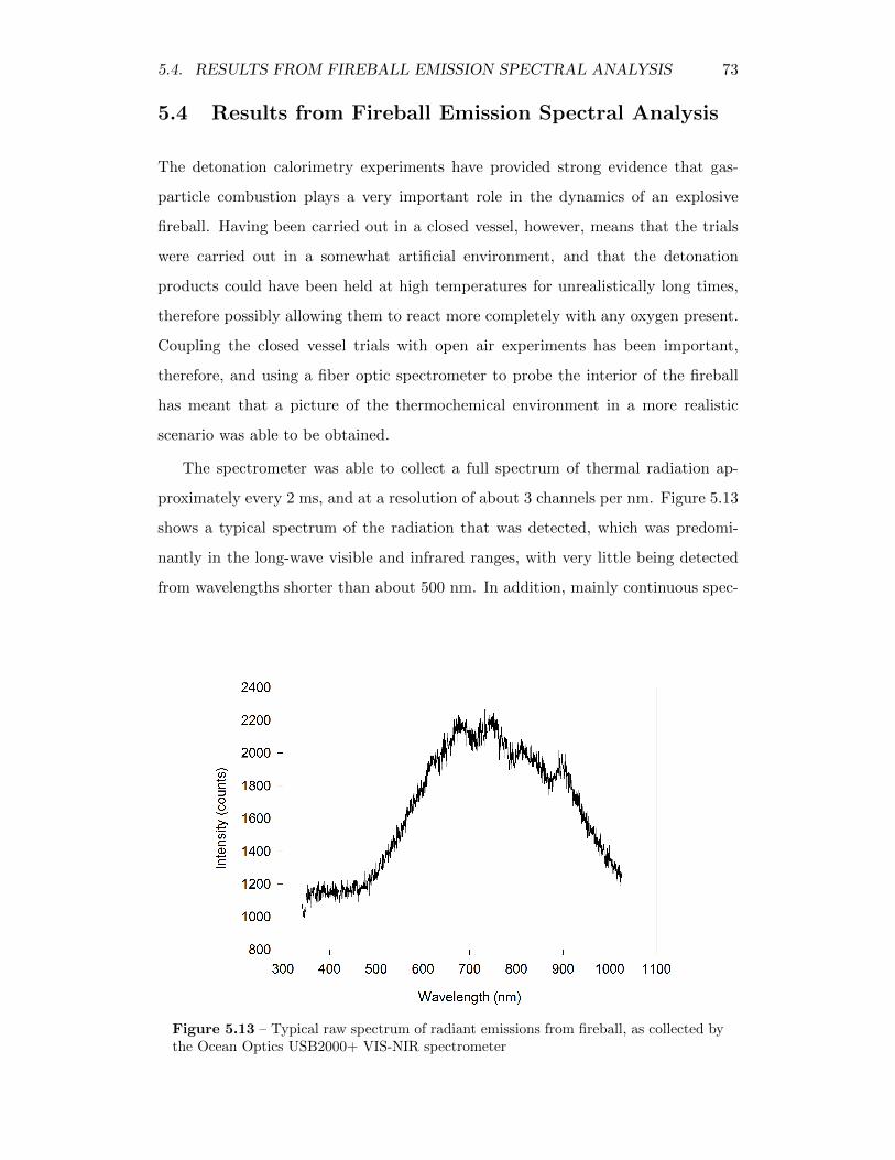
5.4. RESULTS FROM FIREBALL EMISSION SPECTRAL ANALYSIS 73
5.4 Results from Fireball Emission Spectral Analysis
The detonation calorimetry experiments have provided strong evidence that gas-
particle combustion plays a very important role in the dynamics of an explosive
fireball. Having been carried out in a closed vessel, however, means that the trials
were carried out in a somewhat artificial environment, and that the detonation
products could have been held at high temperatures for unrealistically long times,
therefore possibly allowing them to react more completely with any oxygen present.
Coupling the closed vessel trials with open air experiments has been important,
therefore, and using a fiber optic spectrometer to probe the interior of the fireball
has meant that a picture of the thermochemical environment in a more realistic
scenario was able to be obtained.
The spectrometer was able to collect a full spectrum of thermal radiation ap-
proximately every 2 ms, and at a resolution of about 3 channels per nm. Figure 5.13
shows a typical spectrum of the radiation that was detected, which was predomi-
nantly in the long-wave visible and infrared ranges, with very little being detected
from wavelengths shorter than about 500 nm. In addition, mainly continuous spec-
Figure 5.13 – Typical raw spectrum of radiant emissions from fireball, as collected bythe Ocean Optics USB2000+ VIS-NIR spectrometer
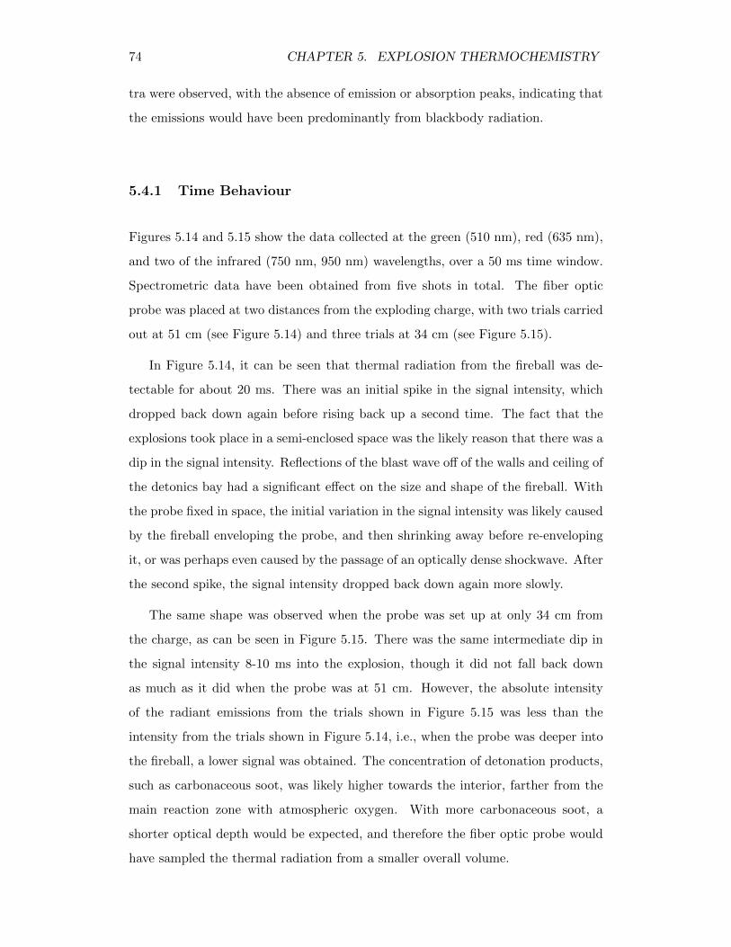
74 CHAPTER 5. EXPLOSION THERMOCHEMISTRY
tra were observed, with the absence of emission or absorption peaks, indicating that
the emissions would have been predominantly from blackbody radiation.
5.4.1 Time Behaviour
Figures 5.14 and 5.15 show the data collected at the green (510 nm), red (635 nm),
and two of the infrared (750 nm, 950 nm) wavelengths, over a 50 ms time window.
Spectrometric data have been obtained from five shots in total. The fiber optic
probe was placed at two distances from the exploding charge, with two trials carried
out at 51 cm (see Figure 5.14) and three trials at 34 cm (see Figure 5.15).
In Figure 5.14, it can be seen that thermal radiation from the fireball was de-
tectable for about 20 ms. There was an initial spike in the signal intensity, which
dropped back down again before rising back up a second time. The fact that the
explosions took place in a semi-enclosed space was the likely reason that there was a
dip in the signal intensity. Reflections of the blast wave off of the walls and ceiling of
the detonics bay had a significant effect on the size and shape of the fireball. With
the probe fixed in space, the initial variation in the signal intensity was likely caused
by the fireball enveloping the probe, and then shrinking away before re-enveloping
it, or was perhaps even caused by the passage of an optically dense shockwave. After
the second spike, the signal intensity dropped back down again more slowly.
The same shape was observed when the probe was set up at only 34 cm from
the charge, as can be seen in Figure 5.15. There was the same intermediate dip in
the signal intensity 8-10 ms into the explosion, though it did not fall back down
as much as it did when the probe was at 51 cm. However, the absolute intensity
of the radiant emissions from the trials shown in Figure 5.15 was less than the
intensity from the trials shown in Figure 5.14, i.e., when the probe was deeper into
the fireball, a lower signal was obtained. The concentration of detonation products,
such as carbonaceous soot, was likely higher towards the interior, farther from the
main reaction zone with atmospheric oxygen. With more carbonaceous soot, a
shorter optical depth would be expected, and therefore the fiber optic probe would
have sampled the thermal radiation from a smaller overall volume.
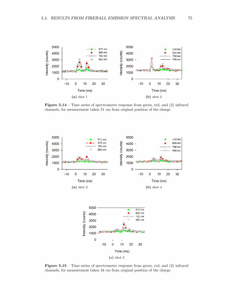
5.4. RESULTS FROM FIREBALL EMISSION SPECTRAL ANALYSIS 75
(a) shot 1 (b) shot 2
Figure 5.14 – Time series of spectrometer response from green, red, and (2) infraredchannels, for measurement taken 51 cm from original position of the charge
(a) shot 3 (b) shot 4
(c) shot 5
Figure 5.15 – Time series of spectrometer response from green, red, and (2) infraredchannels, for measurement taken 34 cm from original position of the charge
76 CHAPTER 5. EXPLOSION THERMOCHEMISTRY
5.4.2 Fireball Emission Spectra and Estimated Temperatures
In each trial, full spectra were collected from the explosive fireballs over about the
20 ms duration where the received signal was strong enough. However, the spectra
recorded by the spectrometer, Is(λ), were related to real spectral irradiance, B(λ),
by the non-linear sensitivity function for the spectrometer, S(λ):
B(λ) = S(λ) · Is(λ) (5.33)
where λ is wavelength.
In order to obtain the latter, the raw spectra were compared to the spectra
obtained from an Ocean Optics LS-1-CAL tungsten halogen lamp, which was used
as a radiometric standard. The spectral response to the light from the lamp was
compared to its known spectral irradiance, as seen in Figure 5.16, and used to define
the sensitivity, S(λ). This way, effects like grating efficiency, CCD response, etc.,
could all be lumped together in the same function:
S(λ) =Bcal(λ)
Is,cal(λ)(5.34)
Figure 5.16 – Signal intensity in spectrometer and real spectral irradiance of LS-1-CALradiometric calibration standard
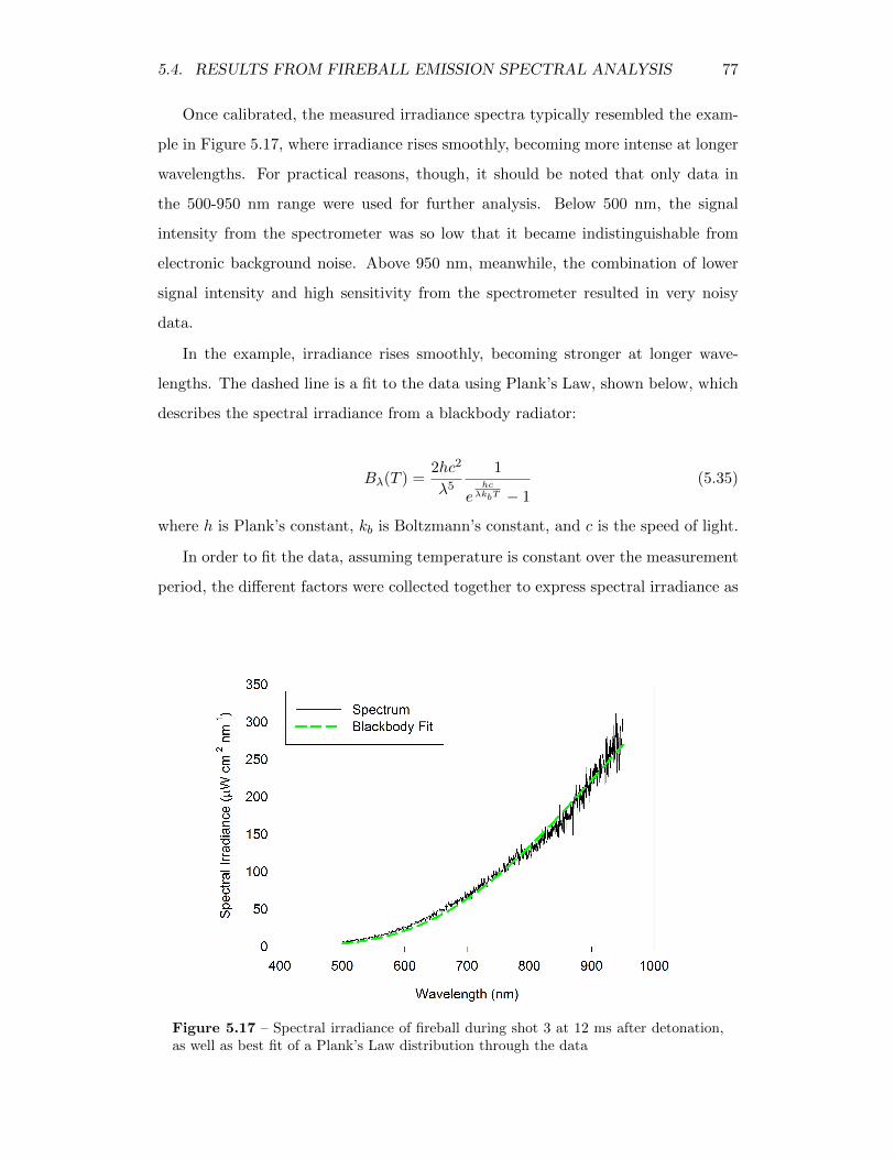
5.4. RESULTS FROM FIREBALL EMISSION SPECTRAL ANALYSIS 77
Once calibrated, the measured irradiance spectra typically resembled the exam-
ple in Figure 5.17, where irradiance rises smoothly, becoming more intense at longer
wavelengths. For practical reasons, though, it should be noted that only data in
the 500-950 nm range were used for further analysis. Below 500 nm, the signal
intensity from the spectrometer was so low that it became indistinguishable from
electronic background noise. Above 950 nm, meanwhile, the combination of lower
signal intensity and high sensitivity from the spectrometer resulted in very noisy
data.
In the example, irradiance rises smoothly, becoming stronger at longer wave-
lengths. The dashed line is a fit to the data using Plank’s Law, shown below, which
describes the spectral irradiance from a blackbody radiator:
Bλ(T ) =2hc2
λ5
1
ehcλkbT − 1
(5.35)
where h is Plank’s constant, kb is Boltzmann’s constant, and c is the speed of light.
In order to fit the data, assuming temperature is constant over the measurement
period, the different factors were collected together to express spectral irradiance as
Figure 5.17 – Spectral irradiance of fireball during shot 3 at 12 ms after detonation,as well as best fit of a Plank’s Law distribution through the data
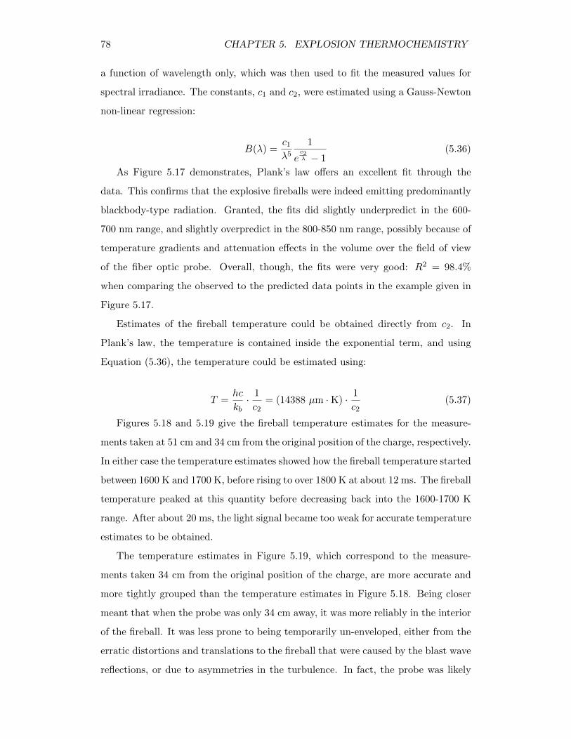
78 CHAPTER 5. EXPLOSION THERMOCHEMISTRY
a function of wavelength only, which was then used to fit the measured values for
spectral irradiance. The constants, c1 and c2, were estimated using a Gauss-Newton
non-linear regression:
B(λ) =c1
λ5
1
ec2λ − 1
(5.36)
As Figure 5.17 demonstrates, Plank’s law offers an excellent fit through the
data. This confirms that the explosive fireballs were indeed emitting predominantly
blackbody-type radiation. Granted, the fits did slightly underpredict in the 600-
700 nm range, and slightly overpredict in the 800-850 nm range, possibly because of
temperature gradients and attenuation effects in the volume over the field of view
of the fiber optic probe. Overall, though, the fits were very good: R2 = 98.4%
when comparing the observed to the predicted data points in the example given in
Figure 5.17.
Estimates of the fireball temperature could be obtained directly from c2. In
Plank’s law, the temperature is contained inside the exponential term, and using
Equation (5.36), the temperature could be estimated using:
T =hc
kb· 1
c2= (14388 µm ·K) · 1
c2(5.37)
Figures 5.18 and 5.19 give the fireball temperature estimates for the measure-
ments taken at 51 cm and 34 cm from the original position of the charge, respectively.
In either case the temperature estimates showed how the fireball temperature started
between 1600 K and 1700 K, before rising to over 1800 K at about 12 ms. The fireball
temperature peaked at this quantity before decreasing back into the 1600-1700 K
range. After about 20 ms, the light signal became too weak for accurate temperature
estimates to be obtained.
The temperature estimates in Figure 5.19, which correspond to the measure-
ments taken 34 cm from the original position of the charge, are more accurate and
more tightly grouped than the temperature estimates in Figure 5.18. Being closer
meant that when the probe was only 34 cm away, it was more reliably in the interior
of the fireball. It was less prone to being temporarily un-enveloped, either from the
erratic distortions and translations to the fireball that were caused by the blast wave
reflections, or due to asymmetries in the turbulence. In fact, the probe was likely
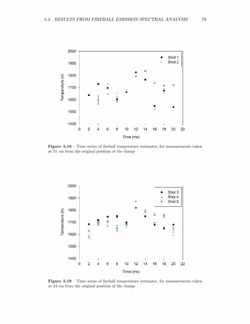
5.4. RESULTS FROM FIREBALL EMISSION SPECTRAL ANALYSIS 79
Figure 5.18 – Time series of fireball temperature estimates, for measurements takenat 51 cm from the original position of the charge
Figure 5.19 – Time series of fireball temperature estimates, for measurements takenat 34 cm from the original position of the charge
80 CHAPTER 5. EXPLOSION THERMOCHEMISTRY
unenveloped by the fireball for a short period when it was located 51 cm from the
original position of the charge, and is likely the cause of the large signal variations
over time.
Despite being closer to the center of the fireball, however, the temperatures that
were measured at 34 cm from the point of detonation were essentially the same,
given the trial-to-trial scatter, as the temperature measurements at 51 cm. The
temperatures from the two measurement sets also evolved in the same way, rising
and falling to the same degree as a function of time. This indicates that heat was
able to transfer throughout the fireball effectively enough to keep the temperature
fairly spatially uniform, either through strong turbulent mixing, or more likely, due
to the high thermal radiation fields.
5.4.3 Relationship with Fireball Thermochemistry
For the detonation products listed for detasheet in Table 5.2, the adiabatic flame
temperature for their complete combustion in air would be about 2150 K. Adiabatic
flame temperature, Ta can be calculated from the heat of afterburn, assuming that
all of the energy released goes into heating the products of complete combustion
from standard state (Cooper, 1996):
∆hab =
∫ Ta
To
cpdT (5.38)
assuming water in the vapour phase, and where cp is the average heat capacity for
all the combustion products. By inverting this expression, one can solve for the
value of Ta, as is shown for detasheet in Appendix G.
The value of 2150 K, it should be noted, cannot be directly compared to the
temperature observations, since it assumes that the detonation products started at
standard temperature and pressure when, in reality, their initial state was unknown.
The system is not adiabatic, at any rate, because a significant amount of thermal
radiation was emitted from the fireball as well.
In addition, the adiabatic flame temperature assumes that reactants are stoi-
chiometrically balanced and react completely, because otherwise, the energy that
is released has to heat more material than necessary. The fact that a lower-than-
expected temperature was observed in the fireball was likely also due to the fact
5.4. RESULTS FROM FIREBALL EMISSION SPECTRAL ANALYSIS 81
that it was fuel rich. Furthermore, the fact that only blackbody radiation was ob-
served, and not any of the prominent lines from excitation bands, implies that the
combustion was still fuel rich. Blackbody radiation in a flame is typically from tiny
particulates of carbonaceous soot, while the gas phase reactions that occur when
fuel/air mixtures are more lean, typically emit light in specific bands that corre-
spond to the excitation peaks of radical intermediates.
The shape of the spectra likely indicated that any combustion that was occurring
was primarily due to the combustion of carbonaceous soot. This fits with the theory
of fireball combustion that has been developed in this chapter, where carbonaceous
soot is consumed first, as its combustion proceeds much more quickly than the
combustion of the gaseous detonation products. Measurements of fireball emission
spectra that were carried out by Goroshin et al. (2006) for TNT and nitromethane
also showed continuous, blackbody-type radiant emissions. These measurements
were taken from the exterior of the fireball, and were integrated over 50 ms, so
cannot be compared directly, although the blackbody curves still indicated that for
non-metalized explosives, combustion in the fireball is primarily due to carbonaceous
soot. It should be noted that the spectra in Goroshin et al. (2006) did show a small
peak at 589 nm, which the authors attributed to sodium. The same peak was
observed in one of the trials in this experimental program, but for the first recorded
spectrum only from shot 2 (see Appendix F), meaning that the peak was likely an
emission from the initial detonation, where the radiation reflected off the ceiling of
the detonics bay to reach the fiber optic probe.
The short optical depth in explosive fireballs can likely be attributed to the
carbon particles as well. The higher the concentration of carbon particles, the lower
the optical depth, and this was likely the reason why, despite the temperature being
roughly the same as a function of time for the two measurement locations, a lower
intensity of radiation was observed when the fiber optic probe was placed only 34 cm
from the point of detonation. With a higher optical density, the thermal emissions
from a smaller volume of the fireball were sampled, and as such a lower intensity
was observed.
As detonation products would be in better contact with atmospheric oxygen,
most of the combustion would likely occur in the outer regions of the fireball. With
82 CHAPTER 5. EXPLOSION THERMOCHEMISTRY
less combustion, the interior would remain more fuel rich, with more carbonaceous
soot, and the optical depth would be shorter. The lower overall intensity of the
collected radiation pointed towards a concentration gradient for the carbonaceous
soot. However, despite this, there was no observable spatial variation in tempera-
ture. Whereas mass transfer relies on slower, physical mechanisms like turbulence
to transport oxygen throughout the fireball, radiant heat transfer occurs much more
quickly, and allows temperatures inside the fireball to be fairly uniform.
5.5 Extension of Thermochemical Model to Heat Re-lease
So far, the reactivity of species in the fireball has been expressed in terms of dimen-
sionless variables. These can be backed out, however, to obtain a function of the
actual heat release in terms of the actual quantity of oxygen that is consumed. As
in Equation 5.28, η can be expressed as a piecewise linear equation in terms of χ as
per:
η =
νo2,g + νo2,c
∆hr,g + ∆hr,c· ∆hr,cνo2,c
· χ χ ≤ νo2,cνo2,g + νo2,c
νo2,g + νo2,c∆hr,g + ∆hr,c
· ∆hr,gνo2,g
· (χ− 1) + 1 χ >νo2,c
νo2,g + νo2,c
(5.39)
For the detonation of explosives alone, without any auxiliary material or en-
trained soil to participate in the fireball, this expression reduces to the following
equation for the heat release per mole of explosives:
Q
nx= hd +
∆hr,cνo2,c
· ∆no2nx
∆no2nx
≤ νo2,c
∆hr,gνo2,g
· ∆no2nx
+ hr,c − hr,gνo2,cνo2,g
∆no2nx
> νo2,c
(5.40)
If several different combustible products can participate in addition to the deto-
nation products, there will be a boosted fireball, where the total heat released as a
function of oxygen consumed is:
5.6. SUMMARY 83
Qboost = nxhd +
∆hr,cνo2,c
·∆no2 ∆no2 ≤ nxνo2,c
∆hr,gνo2,g
·∆no2 + nx
(hr,c − hr,g
νo2,cνo2,g
)∆no2 > nxνo2,c
(5.41)
where:
∆hr,c = (∆hr,c)x +1
nx
∑ni(∆hr,c)i (5.42a)
∆hr,g = (∆hr,g)x +1
nx
∑ni(∆hc −∆hr,c)i (5.42b)
νo2,c = (νo2,c)x +1
nx
∑ni(νo2,c)i (5.42c)
νo2,g = (νo2,g)x +1
nx
∑ni(νo2 − νo2,c)i (5.42d)
5.6 Summary
It has been seen that a theoretical model has been developed that predicts the ther-
mochemistry of an explosion quite well. A fair amount of energy is released during
the initial detonation, but as much or more can be released following this during the
secondary fireball. After all, depending on the oxygen balance, a significant portion
of the detonation products produced by an exploding charge may only be partly
oxidized, and would be able to undergo further combustion in the air.
By looking specifically at the secondary combustion reactions in the fireball, this
chapter has shown that, as the detonation products mix together with atmospheric
oxygen, condensed phase detonation products react much faster than the gaseous
phase detonation products. The closed vessel, detonation calorimetery experiments
have shown this from the relationship between oxygen consumption and heat pro-
duction. This is reinforced by the fact that the thermal emissions observed dur-
ing open-air trials were predominantly from blackbody radiation, with none of the
emission lines that are typically observed in flames undergoing gas-gas combustion
reactions.
Condensed phase detonation products are likely able to react more quickly be-
cause they are able to mix more efficiently with the air in the turbulent fireball. Since
84 CHAPTER 5. EXPLOSION THERMOCHEMISTRY
they are particles, the fact that they have inertia means that when their carrier gas
circulates and changes direction, they will deviate from the streamlines of the gas.
As the gases mix together, the particulates can cross over from fuel-rich detonation
product streams into oxygen-rich air streams. The secondary combustion reactions
are transport limited: whatever species can mix with the air more efficiently will
react first, and so the particulates have an advantage over gas phase products that
allows them to be consumed much more quickly.
Chapter 6
Aerosolization
The residence time of a particle in the atmosphere is largely a function of particle
size. When dealing with hazardous particulates disseminated into the air through
the use of explosives, knowing their size will help determine how far and wide con-
tamination can spread. For particles in the atmosphere, their natural tendency to
settle due to gravity is counteracted by the turbulent motions and viscosity of the
air. Small particulates, because of their large surface to volume ratio, are more
subject to viscous drag, and tend to more closely follow the air in its motions.
A threshold exists where the settling velocity of a particle is on the same order
as the speed of turbulent motions in the air. Below this threshold, turbulence is
strong enough to keep particles well mixed, and ground deposition only occurs when
particles are washed-out due to rainfall, or through by turbulent-inertial deposition
or Brownian diffusion, depending on the particle size. Above this threshold, the
particles are too heavy to stay uniformly suspended, and ground deposition occurs
by gravitational settling. Nominally, this threshold occurs with particles having an
aerodynamic diameter around 50 µm, but is strongly dependent on many factors
like atmospheric conditions (Pasquill, 1974; Friedlander, 2000).
The purpose of this chapter is to discuss how particulates can be generated during
an explosion and subsequently dispersed into the air. Discussions will be centred on
the size of particles that are generated, and will use measurements obtained with
closed vessel experiments to obtain information about soil entrainments effects. The
overarching goal of this chapter is to demonstrate that only a certain portion of the
particles thrown up by a blast will be aerosol-sized, and that the fraction of aerosol-
sized material is heavily influenced by interactions with entrained soil.
85
86 CHAPTER 6. AEROSOLIZATION
6.1 Results from Residual Solids Analysis
All of the soil, soot, and ash remaining after the detonation shots were collected for
analysis. A number of different complementary methods were used with the hope
of measuring different qualities of the residual solids.
Prior to any other analysis, solids were collected from the detonation vessel and
passed through a mechanical sieve. For trials carried out without the addition of soil,
the residual solids were a combination of tiny soot and ash particles, and much larger
fragments from the detonator casing, lead wires, etc. These samples were passed
through a sieve, separating them into two size ranges each, above and below 250 µm.
For trials carried out with soil, the distribution of particle sizes in the residual solids
was much more broad, and so they were separated with the mechanical sieve into
eight particle size ranges.
In subsequent analyses, all of the subsamples from the mechanical sieve separa-
tions were analyzed independently. The particle size distributions from subsamples
with fine enough particulates were measured using a laser diffraction EPCS sys-
tem. SEM images were taken of individual subsamples in order to gain qualitative
information about them, as well as to discriminate between particulates from the
original soil samples and agglomerates that had been formed from smaller ones.
Finally, the elemental composition of subsamples was measured to determine their
lanthanum concentration, and therefore how the powdered target material was dis-
tributed throughout the different size ranges.
6.1.1 Laser Diffraction EPCS Results
The laser diffraction EPCS measurements were taken using a Malvern Spraytec
EPCS system at the University of Ontario Institute of Technology. Measurements
were only taken of samples that were composed of fine enough particles, as the
instrument was only optimized for measurements below 250 µm.
The results are presented in terms of the cumulative mass fraction of material,
Fm(dp), which is defined as a function of particle size, dp, in terms of the mass
frequency distribution, fm(dp), below (Hinds, 1999):
6.1. RESULTS FROM RESIDUAL SOLIDS ANALYSIS 87
Fm(dp) =
∫ dp
0fm(dp)d(dp) (6.1)
Figure 6.1 shows the particle size distributions of the soot and ash produced
by C-4 and detasheet explosives, as measured by the Malvern Spraytec EPCS for
the < 250 µm sieve fraction from trials carried out with explosives only. The data
appear roughly to fall in three groups. The first group has a mass median diameter
(MMD) of approximately 7 µm, and corresponds to the three detasheet trials that
were carried out in the absence of oxygen. The material that makes up these samples
is primarily very fine carbonaceous soot. The second group is from the two C-4 trials
that were also carried out in the absence of oxygen; the MMD was slightly larger at
about 13 µm for these two samples.
Finally, the two samples with the largest average size (one each from a C-4 and
a detasheet trial) were those carried out in an oxygenated atmosphere. The MMD
for these samples was significantly larger at about 33 µm, because all of the fine
carbonaceous soot had been consumed when it reacted with the oxygen that was
present. Any remaining material would have been composed of incombustible ash.
Figure 6.1 – Particle size distribution of soot samples, as obtained from laser diffractionEPCS measurements
88 CHAPTER 6. AEROSOLIZATION
Figure 6.2, meanwhile, shows the measured particle size distribution of the La2O3
powder, as well as residual solids from shots carried out with small amounts of the
powder placed at the end of the charge. The lanthanum oxide powder, prior to being
exposed to a detonation, had an MMD of about 23 µm. The powder was employed
as a target, and about 1.2 g of the material was added to a plastic vial and taped to
the end of explosive charges of C-4. The residual solids from the shot done in the
absence of oxygen are slightly smaller on average than the original lanthanum oxide
powder, with an MMD of about 14 µm. Since the detonated explosive generated a
significant quantity of carbonaceous soot, the lanthanum oxide powder would have
essentially been diluted by the much finer material. As a result, the particle sizes
in this distribution were fairly close to those measured for similar trials carried out
without the La2O3 target (Figure 6.1).
Two of the trials, however, were carried out in the presence of oxygen. There
was an upward shift in the particle size distributions from these two trials, as is
shown in Figure 6.2, with an MMD of approximately 45 µm. Not only is this higher
than the MMD of about 23 µm for the lanthanum oxide powder not exposed to a
Figure 6.2 – Particle size distribution of lanthanum and of the soot from shots carriedout with a lanthanum tracer, as obtained from laser diffraction EPCS measurements
6.1. RESULTS FROM RESIDUAL SOLIDS ANALYSIS 89
detonation, but it is higher than the MMD of about 33 µm for the soot and ash
from the trials with explosives alone.
The Malvern Spraytech EPCS was also used to analyze material from shots
carried out with soil. The residual solids from these trials were separated into
eight different particle size ranges, and the EPCS analysis was carried out on the
0-44 µm, 44-53 µm, and 53-250 µm fractions. These results were combined with
the measurements from the mechanical sieve analysis to built a broad particle size
distribution, and will be shown after the mechanical sieve results are presented.
6.1.2 Sieve Analysis Results
The addition of about 60 g of sand, black earth, or clay increased the overall quantity
of residual solids that had to be processed. In addition, the residual solids contain-
ing soil typically had very broad particle size distributions. Besides the detonator
fragments, there was very little material above 100 µm for shots carried out with
explosives only, but shots carried out with soil had residual solids that spanned in
size to over 1000 µm. As a result, the residual solids from shots carried out with
soil were sieved into eight different particle size ranges prior to further analysis.
All soil types were sieved at the same intensity, and for the same amount of time
( 5 minutes) to ensure that all samples were processed in the same way.
Figures 6.3–6.6 give the particle size distributions from all the C-4 and detasheet
trials carried out with the four types of soil. They all compare the particle size
distribution of the detonation samples to those of the control soil. The figures
show the mass frequency, fi, or the fraction of material collected in each size range,
normalized by the size of the interval. That is to say, each sieve collected particles
over a specific range of sizes, ∆dp, but since the size intervals are not all equal, in
order to be able to compare the numbers obtained for different size ranges side-by-
side, the actual mass fraction, mi/M∞, was divided by the total interval, according
to (Hinds, 1999):
fi = (∆dp)−1 mi
M∞(6.2)
In Figure 6.3, when comparing the particle size distributions of control to detonation-
exposed coarse sand, one can see a significant increase in the fraction of small par-
90 CHAPTER 6. AEROSOLIZATION
ticles. In the control sample, there is a peak in the 297-420 µm range, but there is
very little material smaller than 250 µm. The blast wave from the explosives, how-
ever, fractures the sand particles, breaking them up to produce much smaller ones.
There are even particles in the 0-44 µm range, and particle sizes in the detonation-
exposed samples are fairly uniformly distributed throughout the five smallest size
ranges before dropping back off.
The fine sand particles, whose particle size distributions are shown in Figure 6.4,
are much smaller in comparison to the coarse sand particles. Most of the control
fine sand is in the three size ranges between 53 and 420 µm, with the peak in the 53-
250 µm range. As with the coarse sand, however, there is a significant increase in the
fraction of small particles. The fine sand particles fracture, and break apart in the
same way, and as a result there is a significant shift in the particle size distribution
from large particles, to small ones.
For black earth, the sieve analysis results in Figure 6.5 show that there is not
much difference between the detonation-exposed and control samples. Material is
concentrated below 53 µm, though there is still some in the 53-250 µm, 250-297 µm,
and 297-600 µm ranges. Unlike sand, black earth does not undergo fracturing, and
so there is really no mechanism to generate new small particles. Agglomeration is
inhibited as well, which prevents larger particles from being formed.
For clay, as can be seen in Figure 6.6, the particle size distributions of the control
samples are heavily skewed toward small particles. The peak in the distribution is
in the 0-44 µm range, and there are few control clay particles above 53 µm. For the
detonation-exposed clay, on the other hand, there is a sharp decrease in the amount
of clay in the small size fractions (though clay particles are still more frequently
found in those ranges), and there is a long tail out at larger size fractions.
6.1.3 Construction of Particle Size Distributions
For the trials carried out with soil, two separate measurement techniques were em-
ployed: the mechanical sieve to obtain a broad measure of particle size over the whole
region of interest, and the laser diffraction EPCS to obtain detailed measurements
of particles below 250 µm only. The two measurement techniques are important
for obtaining information about different regions, but neither can cover the whole
6.1. RESULTS FROM RESIDUAL SOLIDS ANALYSIS 91
Figure 6.3 – Particle size distribution of coarse sand samples from sieve analysis
Figure 6.4 – Particle size distribution of fine sand samples from sieve analysis
92 CHAPTER 6. AEROSOLIZATION
Figure 6.5 – Particle size distribution of black earth samples from sieve analysis
Figure 6.6 – Particle size distribution of clay samples from sieve analysis
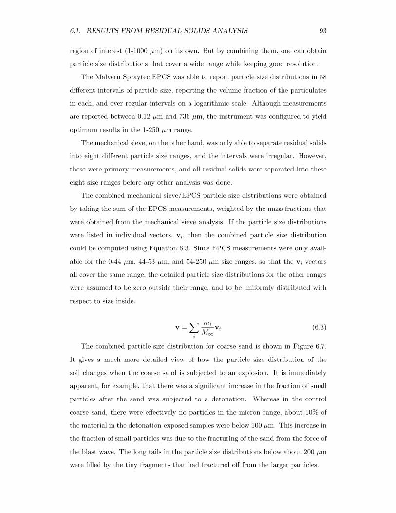
6.1. RESULTS FROM RESIDUAL SOLIDS ANALYSIS 93
region of interest (1-1000 µm) on its own. But by combining them, one can obtain
particle size distributions that cover a wide range while keeping good resolution.
The Malvern Spraytec EPCS was able to report particle size distributions in 58
different intervals of particle size, reporting the volume fraction of the particulates
in each, and over regular intervals on a logarithmic scale. Although measurements
are reported between 0.12 µm and 736 µm, the instrument was configured to yield
optimum results in the 1-250 µm range.
The mechanical sieve, on the other hand, was only able to separate residual solids
into eight different particle size ranges, and the intervals were irregular. However,
these were primary measurements, and all residual solids were separated into these
eight size ranges before any other analysis was done.
The combined mechanical sieve/EPCS particle size distributions were obtained
by taking the sum of the EPCS measurements, weighted by the mass fractions that
were obtained from the mechanical sieve analysis. If the particle size distributions
were listed in individual vectors, vi, then the combined particle size distribution
could be computed using Equation 6.3. Since EPCS measurements were only avail-
able for the 0-44 µm, 44-53 µm, and 54-250 µm size ranges, so that the vi vectors
all cover the same range, the detailed particle size distributions for the other ranges
were assumed to be zero outside their range, and to be uniformly distributed with
respect to size inside.
v =∑i
mi
M∞vi (6.3)
The combined particle size distribution for coarse sand is shown in Figure 6.7.
It gives a much more detailed view of how the particle size distribution of the
soil changes when the coarse sand is subjected to an explosion. It is immediately
apparent, for example, that there was a significant increase in the fraction of small
particles after the sand was subjected to a detonation. Whereas in the control
coarse sand, there were effectively no particles in the micron range, about 10% of
the material in the detonation-exposed samples were below 100 µm. This increase in
the fraction of small particles was due to the fracturing of the sand from the force of
the blast wave. The long tails in the particle size distributions below about 200 µm
were filled by the tiny fragments that had fractured off from the larger particles.
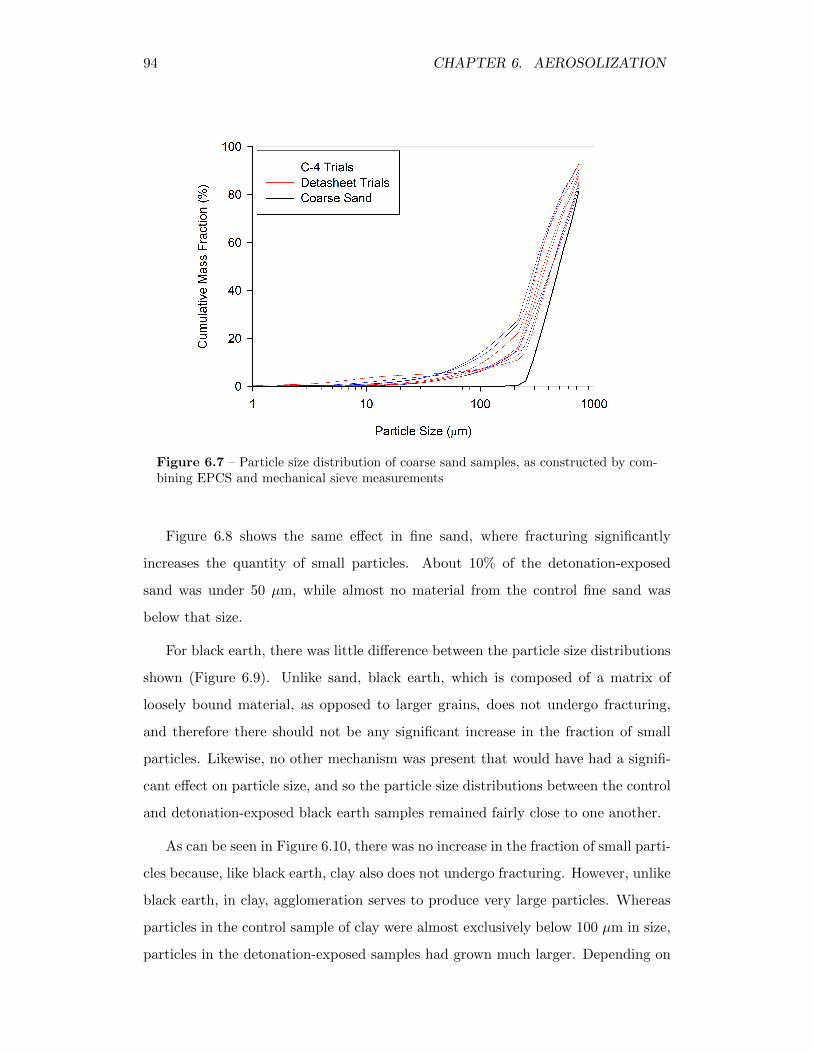
94 CHAPTER 6. AEROSOLIZATION
Figure 6.7 – Particle size distribution of coarse sand samples, as constructed by com-bining EPCS and mechanical sieve measurements
Figure 6.8 shows the same effect in fine sand, where fracturing significantly
increases the quantity of small particles. About 10% of the detonation-exposed
sand was under 50 µm, while almost no material from the control fine sand was
below that size.
For black earth, there was little difference between the particle size distributions
shown (Figure 6.9). Unlike sand, black earth, which is composed of a matrix of
loosely bound material, as opposed to larger grains, does not undergo fracturing,
and therefore there should not be any significant increase in the fraction of small
particles. Likewise, no other mechanism was present that would have had a signifi-
cant effect on particle size, and so the particle size distributions between the control
and detonation-exposed black earth samples remained fairly close to one another.
As can be seen in Figure 6.10, there was no increase in the fraction of small parti-
cles because, like black earth, clay also does not undergo fracturing. However, unlike
black earth, in clay, agglomeration serves to produce very large particles. Whereas
particles in the control sample of clay were almost exclusively below 100 µm in size,
particles in the detonation-exposed samples had grown much larger. Depending on
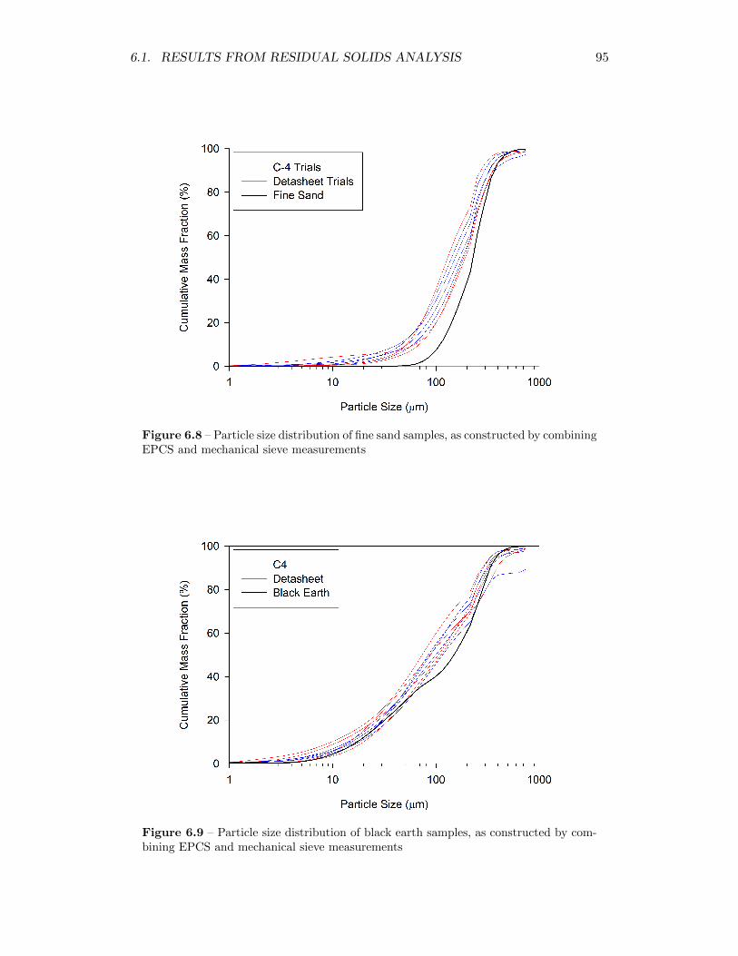
6.1. RESULTS FROM RESIDUAL SOLIDS ANALYSIS 95
Figure 6.8 – Particle size distribution of fine sand samples, as constructed by combiningEPCS and mechanical sieve measurements
Figure 6.9 – Particle size distribution of black earth samples, as constructed by com-bining EPCS and mechanical sieve measurements
96 CHAPTER 6. AEROSOLIZATION
Figure 6.10 – Particle size distribution of clay samples, as constructed by combiningEPCS and mechanical sieve measurements
the conditions, anywhere from 10% to 60% of the clay particles were larger than
100 µm. As will be shown later in this chapter, a trend existed where clay particles
became bigger on average as they were exposed to more and more heat from the
explosive fireball.
6.1.4 Degree of Agglomeration
Agglomeration was observed in the trials carried out with coarse sand, fine sand,
and clay. The particles in control sample of clay were all relatively small, and
the agglomerates that form could be many times – even an order of magnitude or
two – larger. In general terms, for the trials carried out with clay, any particle
in the residual solids that was larger than about 100 µm was almost certainly an
agglomerate.
However, for coarse and fine sand, since the original particles could also be quite
large, they could have been in the same size range as any agglomerates that may
have formed. As a result, the residual solids were a mixture of the original grains
as well as the newly-formed agglomerates, and appeared as a mixture over a range
of different particle sizes.
6.1. RESULTS FROM RESIDUAL SOLIDS ANALYSIS 97
Neither the mechanical sieve nor the Spraytec EPCS system could discriminate
between particles based on type. The only way to do so was visually, by examining
SEM micrographs taken of the residual solids, using the appearance of the particles
to determine whether they were grains or agglomerates, and then measuring the size
and counting the number of the particles in each group.
This was done on all of the coarse and fine sand samples for particles in the
53-250 µm, 250-297 µm, 297-420 µm, 420-600 µm, and 600-841 µm size ranges.
The analyses were limited to these five particle size ranges because the distinction
between agglomerates and single grains began to blur in the smaller particle size
ranges, while obtaining images of ∼ 1 mm and larger particles in the > 841 µm
range with a scanning electron microscope showed particles that were larger than
the field of view of the image.
Images from the SEM were analyzed in Adobe Photoshop, using the FoveaPro 4.0
plug-in, an image analysis toolset that was used to identify individual particles,
separate agglomerates and single grains into different images (based on user inputs),
and measure different aspects of their size and shape. An example of how particles
can be identified and separated is shown in Figure 6.11. Tasks were automated in
Photoshop for reproducibility and speed (see procedure in Appendix D), allowing
79 different images to be processed in total.
(a) original (b) grains (c) agglomerates
Figure 6.11 – Separation and counting sand grains and agglomerates using FoveaProand Photoshop
The measurements of interest from image processing included number of particles
of each type (agglomerates or single grains) and the particle size. The measure of
particle size was the equivalent diameter, deq, which is the diameter of an area-
equivalent circle based on the projected area of the particle (Russ, 2006).
A particular image may have more or less individual particles based on its mag-
nification and the local concentration of particles on the carbon SEM disk on which
98 CHAPTER 6. AEROSOLIZATION
the residual solids were placed. The number fraction, An, of agglomerates to grains
in an image, however, remains consistent and allows results from different images to
be compared directly:
An =naggl
naggl + ngrain(6.4)
where naggl and ngrain are the number of agglomerates and grains, respectively.
However, the value of An is based on number of particles, where the measures
of particle size distribution presented so far have all been based on mass or volume.
Even in a single particle size range, large particles contribute much more mass than
small ones. There would be, for example, a difference in mass of over 100 times
in comparing two particles on the extremes of the 53-250 µm range. The volume
fraction, Av, which incorporates particle size along with number, would therefore be
more useful as a basis of comparison:
Av =
naggl∑i=1
d3eq,i
naggl∑i=1
d3eq,i +
ngrain∑i=1
d3eq,i
(6.5)
In order to obtain consistent statistics, for larger size ranges, multiple micro-
graphs were pooled so that a minimum number of particles could be taken into
account. The error bars in Figures 6.12-6.15 were propagated from√n.
The agglomerate volume fractions for the coarse sand trials are presented in
Figure 6.12. There is a fair amount of variability between different trials because the
degree to which agglomeration occurs depends on time, temperature, and turbulence
in the explosive fireball. In any case, the agglomerate volume fraction is limited to
about 50%, and is in the approximate 0-25% range for most trials.
In fine sand, on the other hand, a much higher fraction of material is composed
of agglomerates, and particularly for large particles. Since fine sand is composed of
smaller particles in general, when large agglomerates form, they take up a bigger
fraction of the large particle size ranges. Figure 6.13, for example, shows that in the
53-250 µm range, agglomerates make up about 5-25% of the material, while above
420 µm, the fraction of agglomerates in the residual solids can approach 100%.
6.1. RESULTS FROM RESIDUAL SOLIDS ANALYSIS 99
Figure 6.12 – Fraction of agglomerates in residual solids from trials with coarse sand
Figure 6.13 – Fraction of agglomerates in residual solids from trials with fine sand
100 CHAPTER 6. AEROSOLIZATION
6.1.5 Lanthanum Composition Analysis
Vials of about 1.2 g each of La2O3 powder were attached to the explosive charges
for eleven of the trials. Three of these trials were carried out with explosives alone,
while the other eight were carried out with soil in the detonation vessel. Lanthanum
concentrations were determined through neutron activation analysis of samples that
were separated into different size ranges with the mechanical sieve.
For the trials carried out without soil, as evidenced in Table 6.1, the lanthanum
was mainly distributed in the particle size fraction < 250 µm. This was to be
expected, since the La2O3 powder particles were well under this size. They mainly
ended up mixed with the soot and ash from the explosions, though some did become
deposited on the detonator fragments and other large particles > 250 µm.
Table 6.1 – Lanthanum concentration in explosive soot and ash residue
Size Range C40204 C40316 C40322
> 250 µm 24± 1 mg·g−1 not enough sample 68± 1 mg·g−1
< 250 µm 232± 6 mg·g−1 249± 2 mg·g−1 279± 2 mg·g−1
In Figure 6.14, the concentration of lanthanum distributed in different particle
size ranges of the detonation-exposed coarse sand is presented. For the trial carried
out in the absence of oxygen, the lanthanum was much more concentrated at low
particle sizes. If the lanthanum oxide powder was simply being diluted by the
other residual solids, and there was little other interaction between particles (besides
some surface contamination), it would be expected that the particle size distribution
of the lanthanum oxide powder would be more or less preserved. For the trial
carried out with an oxygenated atmosphere in the detonation vessel, however, there
was a decrease in the lanthanum concentration at small sizes, and an increase in
concentration at larger sizes. Particle interactions, and likely agglomeration, were
the cause of this as lanthanum became incorporated into larger particles.
The same can be seen in Figure 6.15, where lanthanum was more concentrated
at small particle sizes for the trial carried out under low-oxygen, but then the lan-
thanum shifted towards larger particles for the trial carried out under an oxygenated
atmosphere. In fact, in the latter case, lanthanum was more concentrated among
the larger particles than it was among the smaller ones.
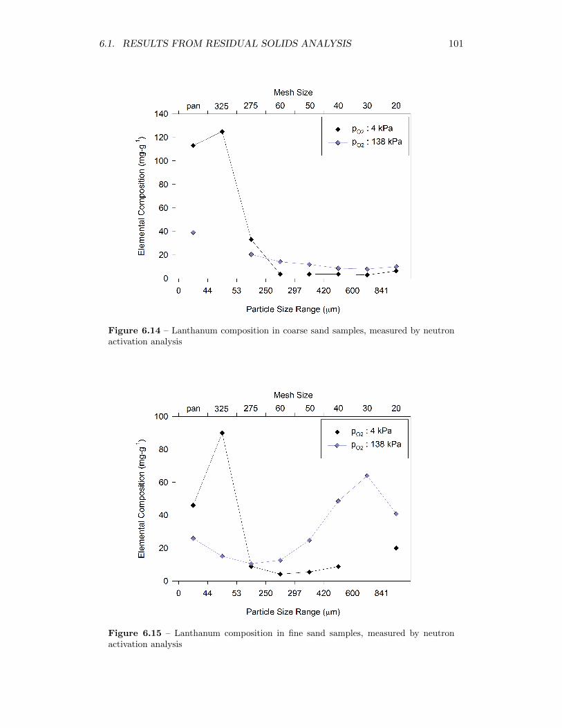
6.1. RESULTS FROM RESIDUAL SOLIDS ANALYSIS 101
Figure 6.14 – Lanthanum composition in coarse sand samples, measured by neutronactivation analysis
Figure 6.15 – Lanthanum composition in fine sand samples, measured by neutronactivation analysis
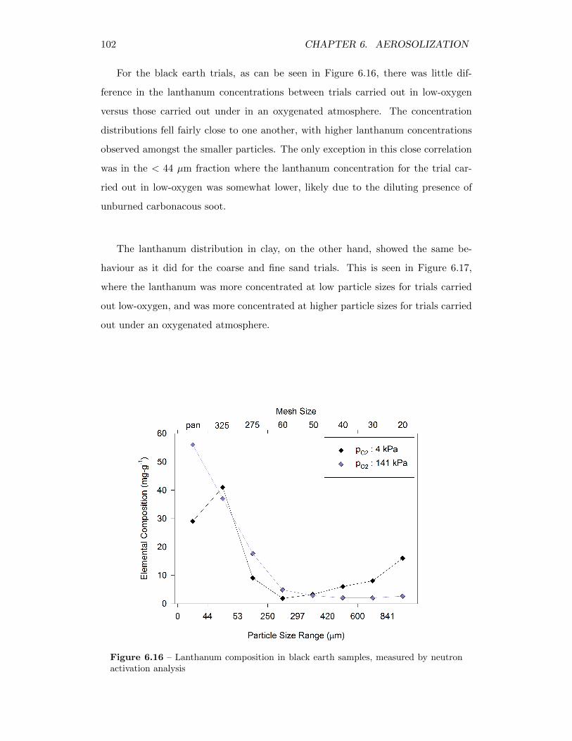
102 CHAPTER 6. AEROSOLIZATION
For the black earth trials, as can be seen in Figure 6.16, there was little dif-
ference in the lanthanum concentrations between trials carried out in low-oxygen
versus those carried out under in an oxygenated atmosphere. The concentration
distributions fell fairly close to one another, with higher lanthanum concentrations
observed amongst the smaller particles. The only exception in this close correlation
was in the < 44 µm fraction where the lanthanum concentration for the trial car-
ried out in low-oxygen was somewhat lower, likely due to the diluting presence of
unburned carbonacous soot.
The lanthanum distribution in clay, on the other hand, showed the same be-
haviour as it did for the coarse and fine sand trials. This is seen in Figure 6.17,
where the lanthanum was more concentrated at low particle sizes for trials carried
out low-oxygen, and was more concentrated at higher particle sizes for trials carried
out under an oxygenated atmosphere.
Figure 6.16 – Lanthanum composition in black earth samples, measured by neutronactivation analysis
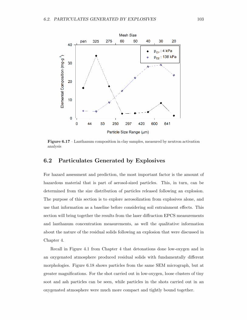
6.2. PARTICULATES GENERATED BY EXPLOSIVES 103
Figure 6.17 – Lanthanum composition in clay samples, measured by neutron activationanalysis
6.2 Particulates Generated by Explosives
For hazard assessment and prediction, the most important factor is the amount of
hazardous material that is part of aerosol-sized particles. This, in turn, can be
determined from the size distribution of particles released following an explosion.
The purpose of this section is to explore aerosolization from explosives alone, and
use that information as a baseline before considering soil entrainment effects. This
section will bring together the results from the laser diffraction EPCS measurements
and lanthanum concentration measurements, as well the qualitative information
about the nature of the residual solids following an explosion that were discussed in
Chapter 4.
Recall in Figure 4.1 from Chapter 4 that detonations done low-oxygen and in
an oxygenated atmosphere produced residual solids with fundamentally different
morphologies. Figure 6.18 shows particles from the same SEM micrograph, but at
greater magnifications. For the shot carried out in low-oxygen, loose clusters of tiny
soot and ash particles can be seen, while particles in the shots carried out in an
oxygenated atmosphere were much more compact and tightly bound together.
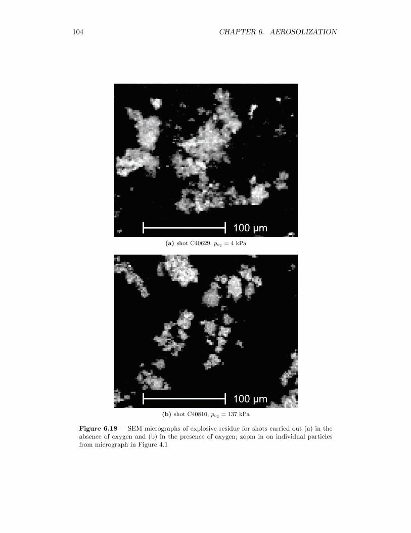
104 CHAPTER 6. AEROSOLIZATION
(a) shot C40629, po2 = 4 kPa
(b) shot C40810, po2 = 137 kPa
Figure 6.18 – SEM micrographs of explosive residue for shots carried out (a) in theabsence of oxygen and (b) in the presence of oxygen; zoom in on individual particlesfrom micrograph in Figure 4.1
6.2. PARTICULATES GENERATED BY EXPLOSIVES 105
This is also seen in Figure 6.19, which shows micrographs obtained from trials
carried out with the addition of the lanthanum oxide powder. As the trial was carried
out in low-oxygen, all of the carbonaceous soot was still present in Figure 6.19a, with
loose clusters of submicron-sized primary soot particles giving the material its light,
flocculent texture. The bright spots in the image are the lanthanum oxide particles,
and are seen to be interspersed with the carbonaceous soot, though not tightly
bound with it. In contrast, in Figure 6.19b, where the shot was carried out in an
oxygenated atmosphere, the particles are seen to be more compact. The higher
magnification in the micrograph was able to show that, with all of the carbonaceous
(a) shot C40204, po2 = 4 kPa
(b) shot C40322, po2 = 137 kPa
Figure 6.19 – SEM micrographs of explosive residue for shots carried out (a) in theabsence of oxygen and (b) in the presence of oxygen
106 CHAPTER 6. AEROSOLIZATION
soot consumed, the ash particles that were left were smaller, more compact, and more
tightly bound together. The particles in the latter case were actually agglomerates,
where incombustible materials, including the lanthanum oxide, fused together to
produce larger particles.
The mass median diameters (MMDs) of the soot and ash from the trials are
shown in Figure 6.20, plotted against the total mass of material collected in the
< 250 µm fraction. In this plot that the MMD of the particle size distributions fell
into two distinct regions. Trials carried out in low-oxygen (two C-4, three detasheet,
one C-4 with La2O3 powder) had smaller MMDs, ranging from about 6 µm to 14 µm.
The trials carried out in and oxygenated atmosphere (one C-4, one detasheet, two
C-4 with La2O3 powder), on the other hand, had MMDs that were much larger. For
ash alone, without any lanthanum oxide powder, the MMD of the residual solids was
about 32 µm, but this was even higher, at around 45 µm, with the trials carried out
with the target. The consequences of this were that, as agglomeration in the fireball
increased the overall particle size, the fraction of material that was aerosol-sized
diminished; the general upward shift in the particle size distribution resulted in a
general decrease in the fraction of small particles.
Figure 6.20 – Mass median diameter of soot and ash, from the < 250 µm fraction
6.2. PARTICULATES GENERATED BY EXPLOSIVES 107
This upward shift in particle size is highlighted in Figure 6.21, which shows
the fraction of material below 50 µm, 10 µm, and 2 µm in size. The plot shows
results from each shot categorically, and basically gives cross sections of the particle
size distribution at three important sizes. As has been discussed already, 50 µm
is the approximate threshold that delineates particles that are aerosol-sized against
those that are too large and heavy to stay suspended in an oxygenated atmosphere.
Particles that are 10 µm and 2 µm in size are well within the aerosol-size range,
but also represent the approximate size range over which particle deposition in the
lungs poses the highest risk.
Figure 6.21 shows that there was a clear distinction between trials that were
carried out in low-oxygen and those carried out in an oxygenated atmosphere. For
those in low-oxygen, 95-98% of the material was under 50 µm, but with the trials in
an oxygenated atmosphere, this was only about 55% and 70% for the trials carried
out with and without the La2O3 target, respectively. Agglomeration of particles in
the fireball significantly shifted the size distribution of particles higher, and signifi-
cantly decreased the fraction of material that ended up as part of particles that were
aerosol-sized.
Figure 6.21 – Fraction of soot and ash under 50 µm, from the < 250 µm fraction; 5shots with MMD< 20 µm were done in low-oxygen, while 4 shots with MMD> 30 µmwere done in an oxygenated atmosphere
108 CHAPTER 6. AEROSOLIZATION
Any initial changes to the explosively dispersed powders were obscured because
of the addition of the fine carbonacous soot, but even so, it was not until they
started to interact in the fireball that the most significant changes to their size was
observed. As was shown in Figure 6.21, in the shots carried out with the lanthanum
oxide powder, about 95% of the material from the shot in low-oxygen was under
50 µm, but only about 55% of the material was less than this for the shots in an
oxygenated atmosphere. In Table 6.2, it can be seen that about 85% of material was
under 50 µm for the shot in low-oxygen, but only an estimated 53% of the target
ended up as part of particles that were aerosol-sized.
Table 6.2 – Lanthanum concentration in soot and ash, from the < 250 µm fraction
TrialPartial PressureOxygen (kPa)
Concentration(mg g−1)
Estimated Fraction< 50 µm
C40204 140 232± 6 84.9%C40316 140 249± 2 53.6%C40322 140 279± 2 54.5%
6.3 Effects on the Particle Size Distributions of Soil
From Section 6.1, it has been seen that the detonation of explosives has a significant
impact on the particle size distributions of soil, and can be broken up to form
smaller ones. Particles can agglomerate back together to form larger ones. There
are a number of competing mechanisms that serve to shift the distribution of particle
sizes either upward or downward. The ultimate goal of this chapter is to identify
factors that influence the aerosolization of hazardous materials. Soil entrainment,
as will be shown in the last section in this chapter, has a significant effect. But since
the detonation of explosives has a strong influence on the particle size distribution
of the soils as well, it is important to first characterize how the soils are affected.
The changes to the particle size distributions of the soils have been quantified
by fitting traditional probability distributions to them, and then noting how the
parameters of those fitted curves change depending on the conditions of the trials.
Depending on the soil type, it may or may not have been possible to fit a single
probability distribution over whole particle size ranges. The soils employed in this
experimental program, and the residual solids collected after the shots, were often
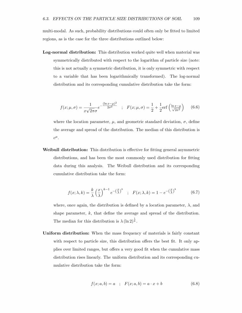
6.3. EFFECTS ON THE PARTICLE SIZE DISTRIBUTIONS OF SOIL 109
multi-modal. As such, probability distributions could often only be fitted to limited
regions, as is the case for the three distributions outlined below:
Log-normal distribution: This distribution worked quite well when material was
symmetrically distributed with respect to the logarithm of particle size (note:
this is not actually a symmetric distribution, it is only symmetric with respect
to a variable that has been logarithmically transformed). The log-normal
distribution and its corresponding cumulative distribution take the form:
f(x;µ, σ) =1
x√
2πσe−
(lnx−µ)2
2σ2 ; F (x;µ, σ) =1
2+
1
2erf(
lnx−µ√2σ2
)(6.6)
where the location parameter, µ, and geometric standard deviation, σ, define
the average and spread of the distribution. The median of this distribution is
eµ.
Weibull distribution: This distribution is effective for fitting general asymmetric
distributions, and has been the most commonly used distribution for fitting
data during this analysis. The Weibull distribution and its corresponding
cumulative distribution take the form:
f(x;λ, k) =k
λ
(xλ
)k−1e−(xλ)
k
; F (x;λ, k) = 1− e−(xλ)k
(6.7)
where, once again, the distribution is defined by a location parameter, λ, and
shape parameter, k, that define the average and spread of the distribution.
The median for this distribution is λ (ln 2)1k .
Uniform distribution: When the mass frequency of materials is fairly constant
with respect to particle size, this distribution offers the best fit. It only ap-
plies over limited ranges, but offers a very good fit when the cumulative mass
distribution rises linearly. The uniform distribution and its corresponding cu-
mulative distribution take the form:
f(x; a, b) = a ; F (x; a, b) = a · x+ b (6.8)
110 CHAPTER 6. AEROSOLIZATION
where a defines the mass frequency. The intercept, b, of the cumulative dis-
tribution is a fitting parameter that depends on the range over which the
distribution is being fit.
It is worth noting that although these probability distributions often fit the data
quite well, there was no fundamental reason why one or the other should have been
used. The soils started with a particular size distribution when they were added to
the vessel, and through a number of complicated mechanisms, the detonation and
fireball changed the mix of particle sizes present. The particle size distribution of
the soil shifted in one direction or the other, and normally became more broad as a
result. It was found that if a particle size distribution could be used to parameterize
the original soil, at least a portion of the residual solids can be parameterized with
the same, albeit shifted, probability distribution. The probability distributions are
useful tools for characterizing the size of soil particles, but the fact that they work
is not necessarily the natural result of some underlying mechanism.
Something that has been observed, however, was that in many cases, the shape
parameter of the fitted distributions was the same from trial to trial when parame-
terizing the residual solids. The shape parameters were different from the original
soil, but for the soil that had been exposed to a detonation, despite greater vari-
ability in the location parameter, the shape parameter was fairly consistent between
trials.
Trial-to-trial consistency in the shape parameter implies that, regardless of the
conditions under which each trial was carried out, there were enough common mech-
anisms that the particle size distributions ended up with the same shape. There may
have still been trial-to-trial variability in the ‘average’ size, but the broadness of the
distribution ended up the same.
A consequence of this was that the particle size distributions of the residual
solids could be made separable. That is to say that they could be divided into
one component that describes the shape, and another component that describes
the ‘average’ size, e.g., the median. This concept comes from the description of self-
similar particle size distributions (Friedlander and Wang, 1966). Without necessarily
assuming that the particle size distributions were self-similar, one could borrow the
mathematics that had been developed to describe self-preserving distributions, and
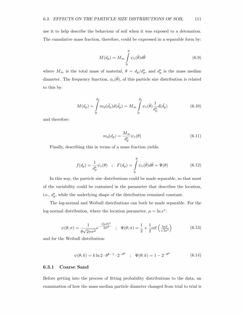
6.3. EFFECTS ON THE PARTICLE SIZE DISTRIBUTIONS OF SOIL 111
use it to help describe the behaviour of soil when it was exposed to a detonation.
The cumulative mass fraction, therefore, could be expressed in a separable form by:
M(dp) = M∞
θ∫0
ψv(θ)dθ (6.9)
where M∞ is the total mass of material, θ = dp/d∗p, and d∗p is the mass median
diameter. The frequency function, φv(θ), of this particle size distribution is related
to this by:
M(dp) =
dp∫0
md(dp)d(dp) = M∞
dp∫0
ψv(θ)1
d∗pd(dp) (6.10)
and therefore:
md(dp) =M∞d∗p
ψv(θ) (6.11)
Finally, describing this in terms of a mass fraction yields:
f(dp) =1
d∗pψv(θ) ; F (dp) =
θ∫0
ψv(θ)dθ = Ψ(θ) (6.12)
In this way, the particle size distributions could be made separable, so that most
of the variability could be contained in the parameter that describes the location,
i.e., d∗p, while the underlying shape of the distribution remained constant.
The log-normal and Weibull distributions can both be made separable. For the
log-normal distribution, where the location parameter, µ = lnx∗:
ψ(θ;σ) =1
θ√
2πσ2e−
(ln θ)2
2σ2 ; Ψ(θ;σ) =1
2+
1
2erf(
ln θ√2σ2
)(6.13)
and for the Weibull distribution:
ψ(θ; k) = k ln 2 · θk−1 · 2−θk ; Ψ(θ; k) = 1− 2−θk
(6.14)
6.3.1 Coarse Sand
Before getting into the process of fitting probability distributions to the data, an
examination of how the mass median particle diameter changed from trial to trial is
112 CHAPTER 6. AEROSOLIZATION
warranted. Figure 6.22 shows the mass median diameter of the coarse sand residual
solids as a function of the total heat released from the trials.
In the original coarse sand, which is represented by the dashed horizontal line,
the mass median diameter was around 500 µm. The mass median diameter of the
residual solids collected from trials done in the absence of oxygen was about the
same, but then, as the soil was exposed to more and more heat from the fireball,
the mass median diameter decreased before plateauing at around 350 µm.
Just to reiterate, for sand, there were two pertinent particle breakup and growth
mechanisms that were identified in Chapter 4 by analyzing SEM micrographs. Frac-
turing was identified to occur, likely due to the force of blast wave from the explosion.
Agglomeration, then, was identified to occur when the sand was exposed to the high
heat of the fireball. With these mechanisms, there should be an initial decrease
in particle size, and then the particle size should go up as particles agglomerate.
The fact that the mass median diameter is going down, however, indicates that a
different, unidentified mechanism must have been in place that was causing this
decrease.
Figure 6.22 – The mass median diameter of coarse sand, comparing the raw materialto sand that has been exposed to a detonation, and as a function of the total heatreleased from the explosions
6.3. EFFECTS ON THE PARTICLE SIZE DISTRIBUTIONS OF SOIL 113
Figure 6.23 shows the total extent of agglomeration in the coarse sand samples
that were exposed to a detonation. It shows the total mass fraction of agglomerates
present in the residual solids, as estimated using the particle counting techniques
of the SEM micrographs described in Section 6.1. Material in the > 841 µm frac-
tion were excluded from this analysis because it was very difficult to obtain good
micrographs in that range. As such, total agglomerate extent is only reported as
the estimated mass fraction of agglomerates from size fractions less than 841 µm.
With the trials carried out in low-oxygen, there was no fireball, and agglomeration
was not observed. However, as the detonation-exposed coarse sand was exposed to
more and more heat from the fireball, there was a marked increase in the extent
of agglomeration. Through the image processing technique, it was estimated that
agglomerates could make up as much as 30% of the of the residual solids, by volume,
for trials with the most energetic fireballs.
Agglomeration was obviously occurring, therefore, and agglomerates were form-
ing in fairly significant quantities. Agglomerates, by their nature, are formed from
smaller particles, and their formation should cause an upward shift in the particle
Figure 6.23 – The overall extent of agglomeration (in all size ranges < 841 µm) in thecoarse sand samples as a function of the total heat released from the explosions
114 CHAPTER 6. AEROSOLIZATION
size distribution. Despite this, though, there was still a decrease in the mass median
diameter. A closer examination of the particle size distribution and its behaviour
with respect to fireball energy, therefore, may be required to investigate why.
The coarse sand, on its own, was composed of relatively large sand grains, with
very few grains smaller than about 250 µm. A log-normal distribution could be
fit to the particle size distribution of the control sample of sand, and offered a fit
that was reasonably close. More specifically, the cumulative log-normal probability
distribution was fit to the cumulative distribution of coarse sand using a Gauss-
Newton non-linear least squares method. The commercial software, SYSTAT 13 was
employed to perform the statistical analysis, and all additional curve fitting carried
out for these analyses were carried out in SYSTAT using the same techniques.
The log-normal fit to the coarse sand particle size distribution is shown in Fig-
ure 6.24a and 6.24c. Figure 6.24b and 6.24d show the particle size distributions
of coarse sand from one trial after being exposed to a detonation. One can see
that the log-normal distribution offered a very good fit to the upper portion of the
distribution, but that there was a long tail that it failed to capture.
It is fairly clear that there were two regimes present in the detonation-exposed
soil (Figure 6.24b and 6.24d), and so separate functions were employed to fit the
distribution in the > 250 µm range and the < 250 µm. As was stated above, a
log-normal distribution was fit in the > 250 µm range. In the < 250 µm range,
although it is distorted because of the log-scale, the distribution was actually fairly
linear. As such, the long tail observed in detonation-exposed samples had a straight
line in the 25-250 µm range fit to it.
The median and geometric standard deviation for the log-normal fits to the
> 250 µm portion of the particle size distributions are shown in Figure 6.25. The
median values of the fits show basically the same trend as the overall median for the
particle size distribution, where the fits to the trials carried out in low-oxygen had
approximately the same median as the control coarse sand, and then the median
decreased to a steady value as oxygen was added to the vessel. But even though
the median values of the log-normal fits changed with fireball energy, the geometric
standard deviations were fairly constant from trial to trial, and consistently above
the geometric standard deviation for the control sample of coarse sand.
6.3. EFFECTS ON THE PARTICLE SIZE DISTRIBUTIONS OF SOIL 115
(a) distribution of the mass fraction ofcoarse sand
(b) distribution of the mass fraction of trialDS0819
(c) cumulative distribution of the mass frac-tion of coarse sand
(d) cumulative distribution of the massfraction of trial DS0819
Figure 6.24 – Log-normal fit of the particle size distribution of coarse sand and twopart uniform (for < 250 µm) / log-normal (for > 250 µm) fit of the particle sizedistribution of coarse sand that has been exposed to a detonation
This last point implies that, despite the fact that there was variability in the
final value for the median, the shapes of the distributions in this range were fairly
consistent. By normalizing the data, therefore, one could try to find an underlying,
dimensionless distribution that defines the shape.
Data in the > 250 µm range were normalized by the median value of their log-
normal fit, and the cumulative mass fractions were plotted against the resulting
dimensionless particle size to produce Figure 6.26. Normalizing these data in this
way collapses the points to a single curve, and fitting a log-normal distribution
through these points produces a probability distribution that is independent of trial
116 CHAPTER 6. AEROSOLIZATION
(a) median (b) geometric standard deviation
Figure 6.25 – Median and geometric standard deviation from log-normal fit to upperportion (> 250 µm) of particle size distributions
Figure 6.26 – Amalgamation of coarse sand particle size distribution in the > 250 µmrange, obtained by normalizing data by the median that was estimated from log-normalfits.
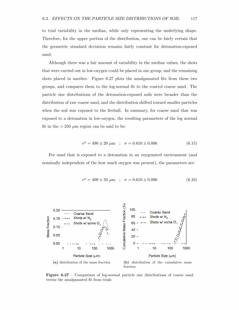
6.3. EFFECTS ON THE PARTICLE SIZE DISTRIBUTIONS OF SOIL 117
to trial variability in the median, while only representing the underlying shape.
Therefore, for the upper portion of the distribution, one can be fairly certain that
the geometric standard deviation remains fairly constant for detonation-exposed
sand.
Although there was a fair amount of variability in the median values, the shots
that were carried out in low-oxygen could be placed in one group, and the remaining
shots placed in another. Figure 6.27 plots the amalgamated fits from these two
groups, and compares them to the log-normal fit to the control coarse sand. The
particle size distributions of the detonation-exposed soils were broader than the
distribution of raw coarse sand, and the distribution shifted toward smaller particles
when the soil was exposed to the fireball. In summary, for coarse sand that was
exposed to a detonation in low-oxygen, the resulting parameters of the log normal
fit in the > 250 µm region can be said to be:
eµ = 490± 20 µm ; σ = 0.610± 0.006 (6.15)
For sand that is exposed to a detonation in an oxygenated environment (and
nominally independent of the how much oxygen was present), the parameters are:
eµ = 400± 50 µm ; σ = 0.610± 0.006 (6.16)
(a) distribution of the mass fraction (b) distribution of the cumulative massfraction
Figure 6.27 – Comparison of log-normal particle size distributions of coarse sandversus the amalgamated fit from trials
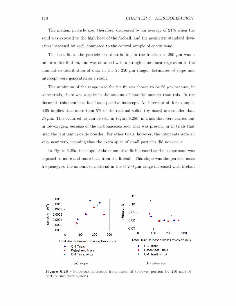
118 CHAPTER 6. AEROSOLIZATION
The median particle size, therefore, decreased by an average of 21% when the
sand was exposed to the high heat of the fireball, and the geometric standard devi-
ation increased by 44%, compared to the control sample of coarse sand.
The best fit to the particle size distribution in the fraction < 250 µm was a
uniform distribution, and was obtained with a straight line linear regression to the
cumulative distribution of data in the 25-250 µm range. Estimates of slope and
intercept were generated as a result.
The minimum of the range used for the fit was chosen to be 25 µm because, in
some trials, there was a spike in the amount of material smaller than this. In the
linear fit, this manifests itself as a positive intercept. An intercept of, for example,
0.05 implies that more than 5% of the residual solids (by mass) are smaller than
25 µm. This occurred, as can be seen in Figure 6.28b, in trials that were carried out
in low-oxygen, because of the carbonaceous soot that was present, or in trials that
used the lanthanum oxide powder. For other trials, however, the intercepts were all
very near zero, meaning that the extra spike of small particles did not occur.
In Figure 6.28a, the slope of the cumulative fit increased as the coarse sand was
exposed to more and more heat from the fireball. This slope was the particle mass
frequency, so the amount of material in the < 250 µm range increased with fireball
(a) slope (b) intercept
Figure 6.28 – Slope and intercept from linear fit to lower portion (< 250 µm) ofparticle size distributions
6.3. EFFECTS ON THE PARTICLE SIZE DISTRIBUTIONS OF SOIL 119
energy. Indeed, the increase is fairly linear. Excluding two of the points, which are
possibly outliers, a linear fit of the particle mass frequency against the total heat
release from the explosions yields:
a = (4.8± 0.3)× 10−6 ·∆Hexpl[kJ ]− (6± 5)× 10−5 (6.17)
Thus, the fraction of particles < 250 µm increased with fireball energy, and this
coincided with a downward shift in the size of particles > 250 µm. There must
have been some mechanism, therefore, that was associated with the fireball and
that served to breakup large particles, and to a degree such that the particle size
distribution shifted downward, despite the fact that agglomeration was occurring
concurrently.
There are a number of factors that may have been responsible. When particles
impact one another, there is a chance that they may fuse together and agglomerate,
but if they hit one another with enough impact, they may break apart instead. Im-
paction of the sand grains against the inner walls of the detonation vessel may be
equally responsible. Alternatively, the large temperature swing in the detonation
vessel may cause thermal stress and cracking to the sand grains. Any of the mecha-
nisms may be the cause, but from the information that is available, there is no way
to determine the mechanism that is responsible.
Some mechanism associated with the fireball, however, must have been respon-
sible for increasing the fraction of particles in the < 250 µm range while taking
material away and reducing the overall size of particles in the > 250 µm range. It
produced a particle size distribution that was bimodal, which followed a uniform
distribution in the < 250 µm range, and a log-normal distribution in the > 250 µm
range. This relationship can be expressed as:
f(dp) =
a dp < 250 µm
1
dp√
2πσ2e−
(ln dp−ln d∗p)2
2σ2 dp ≥ 250 µm
(6.18a)
F (dp) =
a · dp + b dp < 250 µm
1
2+
1
2erf
(ln dp − ln d∗p√
2σ2
)dp ≥ 250 µm
(6.18b)

120 CHAPTER 6. AEROSOLIZATION
In applying Equation 6.18, one could assume that d∗p = 490 µm for trials carried
out in low-oxygen, and d∗p = 400 µm for trials with some oxygen present. The
geometric standard deviation for the log-normal portion of the parameterization
could be assumed to be constant, at σ = 0.61. In the lower portion that follows the
uniform distribution, the particle frequency, a, could be predicted from the heat of
combustion of the explosives, using Equation 6.17.
Using these rules, cumulative particle size distributions were predicted, using
replicate conditions from the trials. The residuals from these predictions are shown
in Figure 6.29. For the most part, the difference between predictions and measure-
ment were less than 10%, and most of the variability was in the > 250 µm range. A
big reason for this variability was because the log-normal distribution is very sensi-
tive to its location parameter. Using only two cases, d∗p = 490 µm or d∗p = 400 µm,
is not the best way to make the predictions, and produces the kind of errors seen in
the residual plot.
However, the variability between the predicted and measured values was much
less in the < 250 µm range. In the range < 250 µm, a relationship was developed
that related the predicted cumulative particle size distribution to the fireball energy,
Figure 6.29 – Residuals from fitting generalized parameterization to the cumulativedistributions of the coarse sand residual solids
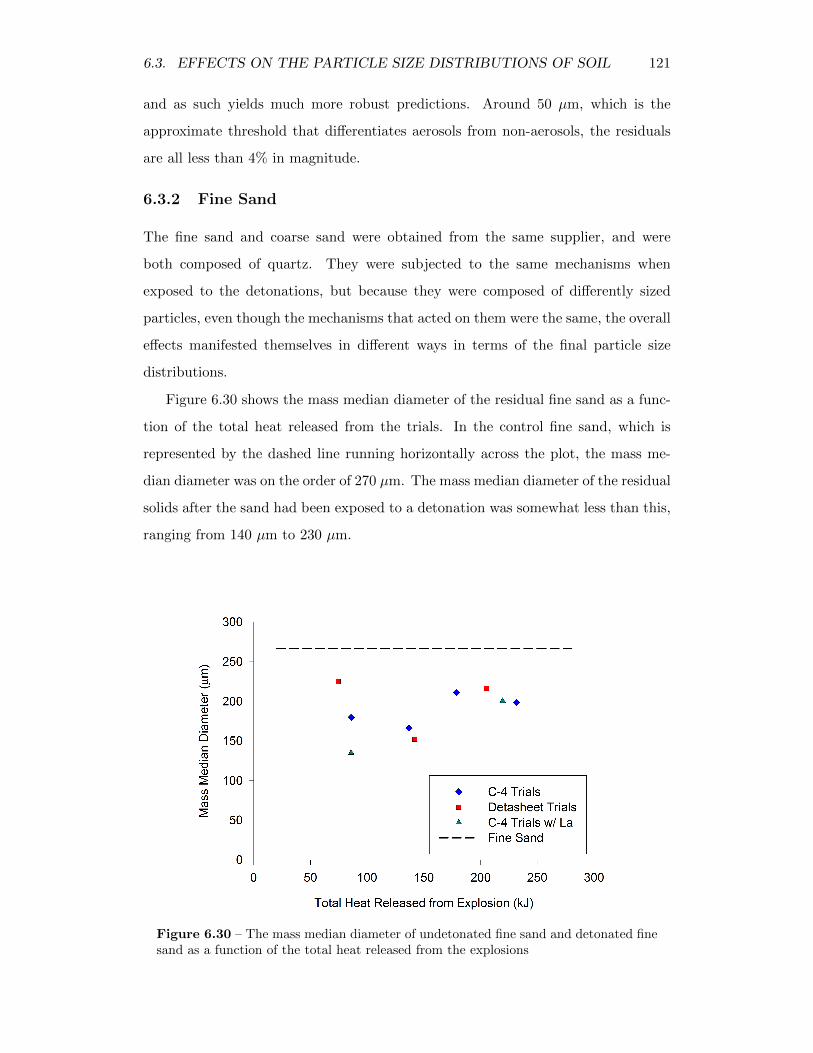
6.3. EFFECTS ON THE PARTICLE SIZE DISTRIBUTIONS OF SOIL 121
and as such yields much more robust predictions. Around 50 µm, which is the
approximate threshold that differentiates aerosols from non-aerosols, the residuals
are all less than 4% in magnitude.
6.3.2 Fine Sand
The fine sand and coarse sand were obtained from the same supplier, and were
both composed of quartz. They were subjected to the same mechanisms when
exposed to the detonations, but because they were composed of differently sized
particles, even though the mechanisms that acted on them were the same, the overall
effects manifested themselves in different ways in terms of the final particle size
distributions.
Figure 6.30 shows the mass median diameter of the residual fine sand as a func-
tion of the total heat released from the trials. In the control fine sand, which is
represented by the dashed line running horizontally across the plot, the mass me-
dian diameter was on the order of 270 µm. The mass median diameter of the residual
solids after the sand had been exposed to a detonation was somewhat less than this,
ranging from 140 µm to 230 µm.
Figure 6.30 – The mass median diameter of undetonated fine sand and detonated finesand as a function of the total heat released from the explosions
122 CHAPTER 6. AEROSOLIZATION
This behaviour was somewhat different from that seen for coarse sand. For the
trials carried out in low-oxygen, the mass median diameter of coarse sand was more
or less unchanged from that in the control sample, but for the fine sand, the mass
median diameters of the residual solids were both lower, and more variable.
After the initial detonation, when the fine sand was exposed to heat from the
fireball, the mass median diameter started out low, but then rose to a plateau at
around 200 µm. This is in contrast to the coarse sand, where the mass median
diameter decreased to a steady value.
Figure 6.31 shows the total extent of agglomeration in the fine sand samples
that were exposed to a detonation. Once again, it only shows the total agglomerate
extent is only reported as the estimated mass fraction of agglomerates from size
fractions less than 841 µm. No agglomeration was observed in trials carried out in
low-oxygen, but the extent then steadily rises to upwards of 30% when the sand was
exposed to heat from the fireball.
Once again, agglomerates ended up forming in fairly large proportion when the
sand was exposed to the high heat of the fireball. In fact, the rise in total agglom-
Figure 6.31 – The overall extent of agglomeration (in all size ranges < 841 µm) in thefine sand samples as a function of the total heat released from the explosions
6.3. EFFECTS ON THE PARTICLE SIZE DISTRIBUTIONS OF SOIL 123
eration extent was almost identical to the rise observed in coarse sand. In this case,
it was likely that the secondary rise in mass median diameter that was observed
was because of agglomeration. But, at the same time, the increase in agglomeration
extent was not well correlated with the behaviour of the mass median diameter.
If agglomeration were the only mechanism of importance in the fireball, then one
would expect the mass median diameter of particles to go up in the same way as
the total agglomeration extent. Since this was not the case, however, it implies,
similarly to coarse sand, that there must have been some mechanism in addition to
agglomeration that also affected particle size in the fireball.
Even though all the different underlying mechanisms cannot be explicitly identi-
fied, however, some meaningful relationships can still be identified by taking a closer
examination of the particle size distributions. It was found that the log-normal
probability distribution did the best job parameterizing coarse sand. However, the
particle size distribution of fine sand, in addition to being smaller overall, was also
skewed in a different way. The fine sand, it was found, could be parameterized by
a single distribution, the Weibull distribution, that was valid over the whole range
of the particle sizes and that fit the unaffected material and the detonation-exposed
material equally well.
Figure 6.32 shows the Weibull distribution fit to the fine sand data. Figures 6.32a
and 6.32c show the distribution of the mass fraction and the cumulative distribution
of the control sample of fine sand, while Figures 6.32b and 6.32d show the distribu-
tion from one trial after being exposed to a detonation. In both cases, the Weibull
distribution offers an excellent fit to the data, though it is immediately apparent
that in the detonation-exposed samples, the distribution is much more broad and
spread out.
The scale and shape parameters for the Weibull fits are shown in Figure 6.33.
The scale parameter fits show the same trend as the mass median diameter, in
that they rose toward a plateau after initially decreasing with increasing fireball
energy, but all the while being systematically below the scale parameter for the
control sample of fine sand. This sort of behaviour would be expected because, for
the Weibull distribution, the scale parameter is linearly related to the median by
x∗ = λ(ln 2)1k .
124 CHAPTER 6. AEROSOLIZATION
(a) distribution of the mass fraction of finesand
(b) distribution of the mass fraction of trialDS0831
(c) cumulative distribution of the mass frac-tion of fine sand
(d) cumulative distribution of the massfraction of trial DS0831
Figure 6.32 – Weibull fit of control and detonation-exposed fine sand particle sizedistributions
Even though the scale parameter, λ, did appear to have some relationship with
fireball energy, the shape parameter, k, remained fairly constant from trial to trial,
and was systematically below the shape parameter for the control sample of sand.
This was the same for coarse sand, where the geometric standard deviation, which is
effectively the shape parameter for a log-normal distribution, was also fairly constant
from trial to trial.
So, even though there was variability in the scale parameter of the fine sand
particle size distributions, the shapes of the distributions were fairly constant. The
data could therefore be normalized to try to find an underlying, dimensionless dis-
tribution that defines the shape.
6.3. EFFECTS ON THE PARTICLE SIZE DISTRIBUTIONS OF SOIL 125
(a) scale parameter (b) shape parameter
Figure 6.33 – Shape and scale parameters from Weibull fits of soil from trials withfine sand
Data from the fine sand shots were normalized by the median value of their fitted
Weibull distributions, and the cumulative mass fractions were plotted against the
resulting dimensionless particle size to produce Figure 6.34. Normalizing the data
this way collapsed the points to a single curve, and fitting a Weibull distribution
through these points produced a probability distribution that was independent of
trial to trial variability in the scale parameter, while both preserving the underlying
shape and confirming that it was the representative one for all of the trials.
Despite the variability in the scale parameters, one could group them all to-
gether to demonstrate how, on average, the particle size distribution shifted after
the sand was exposed to a detonation. Unlike the case for coarse sand, there was
not enough difference in the scale parameter to separate the soil from shots carried
out in low-oxygen from the remaining trials. Figure 6.35 plots the amalgamated fit
and compares it to the Weibull distribution fit to the control fine sand. The particle
size distribution of the detonation-exposed soil is broader than the distribution of
the control fine sand, and the distribution shifts toward smaller particles when the
soil is exposed to the fireball. Taking the shape parameter as the average of all the
trials, the Weibull parameters were:
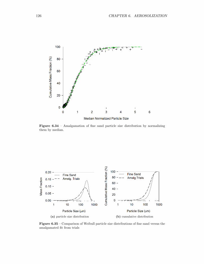
126 CHAPTER 6. AEROSOLIZATION
Figure 6.34 – Amalgamation of fine sand particle size distribution by normalizingthem by median.
(a) particle size distribution (b) cumulative distribution
Figure 6.35 – Comparison of Weibull particle size distributions of fine sand versus theamalgamated fit from trials
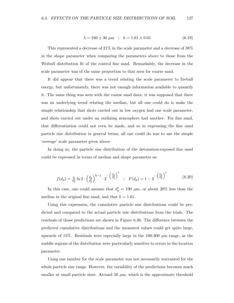
6.3. EFFECTS ON THE PARTICLE SIZE DISTRIBUTIONS OF SOIL 127
λ = 240± 30 µm ; k = 1.61± 0.01 (6.19)
This represented a decrease of 21% in the scale parameter and a decrease of 38%
in the shape parameter when comparing the parameters above to those from the
Weibull distribution fit of the control fine sand. Remarkably, the decrease in the
scale parameter was of the same proportion to that seen for coarse sand.
It did appear that there was a trend relating the scale parameter to fireball
energy, but unfortunately, there was not enough information available to quantify
it. The same thing was seen with the coarse sand data: it was supposed that there
was an underlying trend relating the median, but all one could do is make the
simple relationship that shots carried out in low oxygen had one scale parameter,
and shots carried out under an oxidizing atmosphere had another. For fine sand,
that differentiation could not even be made, and so in expressing the fine sand
particle size distribution in general terms, all one could do was to use the simple
‘average’ scale parameter given above.
In doing so, the particle size distribution of the detonation-exposed fine sand
could be expressed in terms of median and shape parameter as:
f(dp) = kd∗p
ln 2 ·(dpd∗p
)k−1· 2−(dpd∗p
)k; F (dp) = 1− 2
−(dpd∗p
)k(6.20)
In this case, one could assume that d∗p = 190 µm, or about 20% less than the
median in the original fine sand, and that k = 1.61.
Using this expression, the cumulative particle size distributions could be pre-
dicted and compared to the actual particle size distributions from the trials. The
residuals of those predictions are shown in Figure 6.36. The difference between the
predicted cumulative distributions and the measured values could get quite large,
upwards of 15%. Residuals were especially large in the 100-300 µm range, as the
middle regions of the distribution were particularly sensitive to errors in the location
parameter.
Using one number for the scale parameter was not necessarily warranted for the
whole particle size range. However, the variability of the predictions becomes much
smaller at small particle sizes. Around 50 µm, which is the approximate threshold
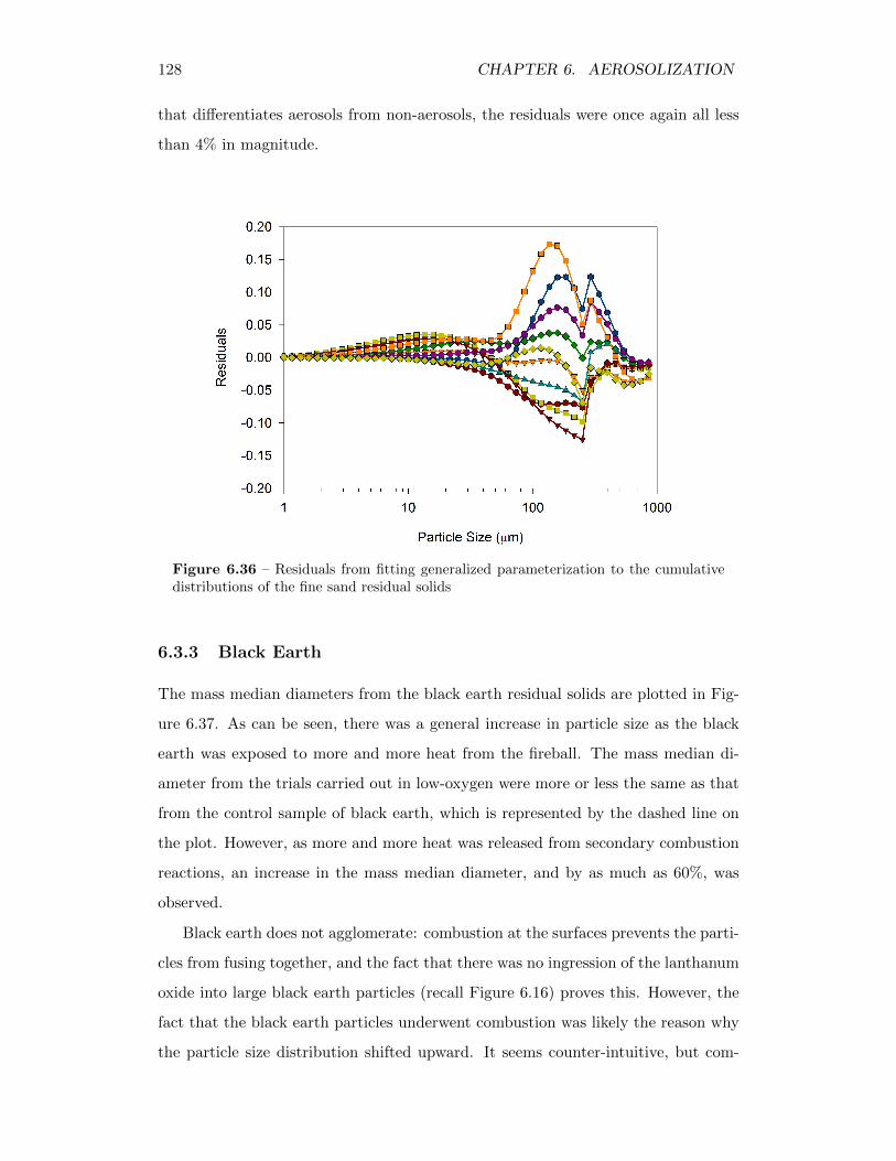
128 CHAPTER 6. AEROSOLIZATION
that differentiates aerosols from non-aerosols, the residuals were once again all less
than 4% in magnitude.
Figure 6.36 – Residuals from fitting generalized parameterization to the cumulativedistributions of the fine sand residual solids
6.3.3 Black Earth
The mass median diameters from the black earth residual solids are plotted in Fig-
ure 6.37. As can be seen, there was a general increase in particle size as the black
earth was exposed to more and more heat from the fireball. The mass median di-
ameter from the trials carried out in low-oxygen were more or less the same as that
from the control sample of black earth, which is represented by the dashed line on
the plot. However, as more and more heat was released from secondary combustion
reactions, an increase in the mass median diameter, and by as much as 60%, was
observed.
Black earth does not agglomerate: combustion at the surfaces prevents the parti-
cles from fusing together, and the fact that there was no ingression of the lanthanum
oxide into large black earth particles (recall Figure 6.16) proves this. However, the
fact that the black earth particles underwent combustion was likely the reason why
the particle size distribution shifted upward. It seems counter-intuitive, but com-
6.3. EFFECTS ON THE PARTICLE SIZE DISTRIBUTIONS OF SOIL 129
Figure 6.37 – The mass median diameter of undetonated black earth and detonatedblack earth as a function of the total heat released from the explosions
bustion is a surface effect. To illustrate, if 1 µm is eroded from the surface of a
200 µm particle, it is still 198 µm in diameter afterwards. If 1 µm is eroded from
the surface of a 2 µm particle, on the other hand, it will completely disappear. As
the surface to volume ratio is higher in smaller particles, they will preferentially be
consumed over larger particles. The result is that the average particle size increases,
even though the size of individual particles decreases, and this was the likely cause
behind the increase in mass median diameter that was observed with black earth.
By examining the particle size distributions as a whole, the results of this effect
and its relationship with the total heat released from the explosions could be better
quantified. As was done for coarse and fine sand, probability distributions were
fit to the particle size distribution of black earth, and by observing how the fitting
parameters changed, shifts in the distributions could be quantified. The Weibull dis-
tribution worked well at parameterizing fine sand, and it was found that it provided
a reasonably good fit for parameterizing black earth as well.
One of the challenges associated with parameterizing the black earth, however,
was that it had some bimodal characteristics, although the two ‘modes’ overlapped
and were difficult to deconvolute. For example shown in Figure 6.38, this can be
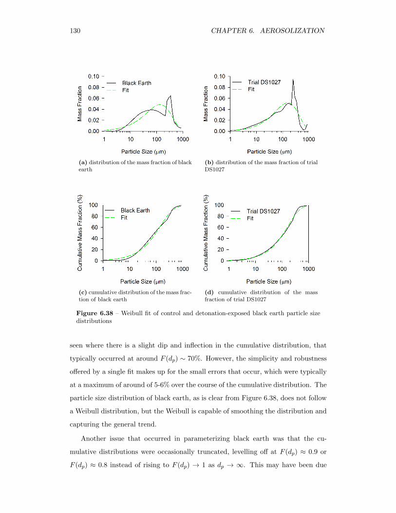
130 CHAPTER 6. AEROSOLIZATION
(a) distribution of the mass fraction of blackearth
(b) distribution of the mass fraction of trialDS1027
(c) cumulative distribution of the mass frac-tion of black earth
(d) cumulative distribution of the massfraction of trial DS1027
Figure 6.38 – Weibull fit of control and detonation-exposed black earth particle sizedistributions
seen where there is a slight dip and inflection in the cumulative distribution, that
typically occurred at around F (dp) ∼ 70%. However, the simplicity and robustness
offered by a single fit makes up for the small errors that occur, which were typically
at a maximum of around of 5-6% over the course of the cumulative distribution. The
particle size distribution of black earth, as is clear from Figure 6.38, does not follow
a Weibull distribution, but the Weibull is capable of smoothing the distribution and
capturing the general trend.
Another issue that occurred in parameterizing black earth was that the cu-
mulative distributions were occasionally truncated, levelling off at F (dp) ≈ 0.9 or
F (dp) ≈ 0.8 instead of rising to F (dp) → 1 as dp → ∞. This may have been due
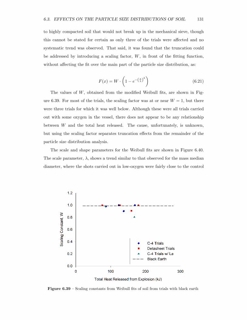
6.3. EFFECTS ON THE PARTICLE SIZE DISTRIBUTIONS OF SOIL 131
to highly compacted soil that would not break up in the mechanical sieve, though
this cannot be stated for certain as only three of the trials were affected and no
systematic trend was observed. That said, it was found that the truncation could
be addressed by introducing a scaling factor, W , in front of the fitting function,
without affecting the fit over the main part of the particle size distribution, as:
F (x) = W ·(
1− e−( xλ)k)
(6.21)
The values of W , obtained from the modified Weibull fits, are shown in Fig-
ure 6.39. For most of the trials, the scaling factor was at or near W = 1, but there
were three trials for which it was well below. Although these were all trials carried
out with some oxygen in the vessel, there does not appear to be any relationship
between W and the total heat released. The cause, unfortunately, is unknown,
but using the scaling factor separates truncation effects from the remainder of the
particle size distribution analysis.
The scale and shape parameters for the Weibull fits are shown in Figure 6.40.
The scale parameter, λ, shows a trend similar to that observed for the mass median
diameter, where the shots carried out in low-oxygen were fairly close to the control
Figure 6.39 – Scaling constants from Weibull fits of soil from trials with black earth
132 CHAPTER 6. AEROSOLIZATION
(a) scale parameter (b) shape parameter
Figure 6.40 – Shape and scale parameters from Weibull fits of soil from trials withblack earth
sample of black earth, and then increased as more oxygen was added to the vessel.
The rise, in fact, was fairly linear, and fitting a line through the points yielded:
λ = β1 ·∆Hexpl + βo = (0.49± 0.09) ·∆Hexpl + (100± 10) (6.22)
This linear fit, though, excludes the two trials that were carried out with the
La2O3 powder. Although they run parallel, the two points were statistical outliers
below the other values, possibly because the La2O3 mixed in with the soil shifted
its size distributions downward slightly.
Although there was an upward trend in the scale parameter, the shape parame-
ter, k, neither rose nor fell as a function of the total heat release from the explosions.
The values of k from the trials were all consistently higher than the shape parameter
for the black earth that had not been exposed to a detonation. That being said,
there was a fair degree of scatter in the data points. The 95% confidence interval for
the values of k from the trials was (0.82,1.15), and at 0.87, the shape parameter for
the control black earth was within this range. So even though there may have been
a slight increase in the shape parameters after the black earth was exposed to the
detonations, implying that the particle size distributions became slightly narrower,

6.3. EFFECTS ON THE PARTICLE SIZE DISTRIBUTIONS OF SOIL 133
the changes were not statistically significant, and for all intents and purposes there
was no change in the shape parameter from pre- to post-detonation.
Furthermore, because the shape parameters were all relatively consistent, it im-
plied that the shape and scale may be separable. The data could therefore be
normalized in order to find a dimensionless distribution that defined the shape. The
particle size could be normalized by the median (θ = dp/d∗p, where d∗p = λ ln(2)
1k ),
and the cumulative distribution could be normalized by the scaling factor so the
truncation effects would not interfere with the analysis (i.e. F (θ)/W ). Points from
the dimensionless cumulative distributions that resulted are shown in Figure 6.41.
The normalized data all fell on a single curve, and fitting a Weibull distribution
through these points produced a probability distribution that contained the shape
information, while being independent of particle size. In addition, since Figure 6.41
includes both the particle size distributions from the trials as well as from the control,
it shows that the probability distribution represented the fundamental shape for
both. It was found, therefore, that the shape parameter for black earth, regardless
of whether it was exposed to a detonation or not, was k = 0.974± 0.007.
Figure 6.41 – Amalgamation of black earth particle size distribution by normalizingthem by median.
134 CHAPTER 6. AEROSOLIZATION
Using the information gained so far in the analysis, a general expression could
be developed to parameterize the particle size distribution of black earth. There
were two parts to this relationship. First, the mass median diameter of the particle
size distribution could be predicted from the following, which used the information
gained from the linear fit to the scale parameter (Equation 6.22), knowing that
d∗p = λ(ln 2)1k :
d∗p = (0.34± 0.06) ·∆Hexpl + (70± 9) (6.23)
Since Equation 6.22 did not apply to the shots with lanthanum oxide, the ex-
pression above cannot be used. However, since the values of λ appeared parallel to
the trend in the other trials, only shifted downward, the intercept can be lowered so
that they fit through the points while the slope is kept constant to yield:
d∗p = (0.34± 0.06) ·∆Hexpl + (47± 9) (6.24)
Once the mass median diameter was known, the overall particle size distribution
could be predicted from:
f(dp) = kd∗p
ln 2 ·(dpd∗p
)k−1· 2−(dpd∗p
)k; F (dp) = 1− 2
−(dpd∗p
)k(6.25)
This expression allowed the particle size distribution of black earth to be pre-
dicted as a function of the total heat released from an explosion. The performance
of this expression could be evaluated by comparing predictions of the cumulative
distributions to the measurements on which the parameterization was built. The
residuals of those predictions are shown in Figure 6.42.
The magnitude of the residuals seen in Figure 6.42 are primarily because a single
Weibull distribution was used for the sake of simplicity, in spite of the bimodal
nature of black earth. The parameterization systematically underpredicts in the
200-400 µm range as a result, but even so, the residuals were all under 8%, and
overall, the parameterization that was developed was fairly robust in its predictions.
6.3. EFFECTS ON THE PARTICLE SIZE DISTRIBUTIONS OF SOIL 135
Figure 6.42 – Residuals from fitting generalized parameterization to the cumulativedistributions of the black earth residual solids
6.3.4 Clay
Figure 6.43 shows the mass median diameter of the clay particulates after they had
been exposed to a detonation. The plot shows how the MMD rose considerably
as a function of the total heat released from the trials. Particles in the residual
solids were far larger than those from the control sample of clay, whose MMD is
represented by the dashed line at the bottom of the plot. The upward trend is fairly
clear, with the exception of one point from shot C41005, which appears to be an
outlier, though the reasons why it is an outlier is unclear.
As identified in Chapter 4, the growth of particles was primarily due to agglom-
eration. Although soil compaction, where the blast wave compressed the clay into
a hard matrix, may have been another factor, the formation of the very large parti-
cles was almost exclusively due to agglomeration. Figure 6.44 shows an example of
the particles seen in the size range between 250-297 µm, where the residual solids
transition to being composed almost exclusively of agglomerates. A mix of parti-
cles is seen in this micrograph, but above this size, the only particles present are
agglomerates.
136 CHAPTER 6. AEROSOLIZATION
Figure 6.43 – The mass median diameter of the control and detonation-exposed clayas a function of the total heat released from the explosions
Figure 6.44 – SEM micrograph of residual clay in the 250-297 µm range following shotC41005
Assuming that all the particles > 250 µm can be treated as agglomerates, the
total extent of agglomeration could be obtained directly from the fraction of clay
residual solids above that size. The extent of agglomeration is shown, therefore, in
Figure 6.45, which shows that there was a linear increase in agglomeration extent
as the clay was exposed to more and more heat from the fireball. At the high end,
upwards of 70% of the original mass of clay ended up as part of agglomerates.
6.3. EFFECTS ON THE PARTICLE SIZE DISTRIBUTIONS OF SOIL 137
Figure 6.45 – The overall extent of agglomeration, assuming all particles above 250 µmare agglomerates, as a function of the total heat released from the explosions
Excluding the outlier point, a linear regression of the data in Figure 6.45 yielded
the following expression, which relates the fraction of material > 250 µm to the total
heat released from the explosions:
Faggl = β1 ·∆Hexpl + βo = (0.0043± 0.0005) ·∆Hexpl + (−0.22± 0.06) (6.26)
This resulted in a remarkably good fit over the range of the data. But just as a
caution, it would not be valid to extrapolate the linear fit into higher agglomeration
extents. No matter how much energy is released from the explosions, the fraction of
material > 250 µm will never exceed 100%, and as such the linear relationship must
level off at some point.
In Figure 6.46, however, when comparing the mass median diameter to the frac-
tion of material > 250 µm, an even more tightly grouped relationship is seen. Except
for three points near the bottom of the scale, there was a very strong correlation
between the mass median diameter and the extent of agglomeration. Even the point
that was an outlier, when relating particle size to heat release, fell within this group-
ing. On a semi-log plot, the correlation is a straight line, suggesting that there was
138 CHAPTER 6. AEROSOLIZATION
Figure 6.46 – Correlation between the mass median diameter and extent of agglom-eration
an exponential relationship between the median particle size and the total amount
of material that was able to form agglomerates.
The three points that did not follow this trend were the ones from trials that
were carried out in low-oxygen. From the set of SEM micrographs, agglomerate
formation was never observed when detonation vessel’s atmosphere was essentially
only nitrogen, and so where no fireball occurs. Soil compaction did play a part
in making larger particles, as when the clay compacted into a hard matrix, the
mechanical sieve was not able to break it back up completely to its original state.
The result was that some of the clay ended up as part of particles that were larger
than they otherwise would have been, though compaction did not allow for the
production particles that were nearly as large as agglomeration was able to produce.
Excluding the data from the three shots that were carried out in low-oxygen, a re-
lationship between the mass median diameter and the fraction of material > 250 µm
could be developed. Taking a linear regression of the logarithmically transformed
data, the following exponential relationship could be developed:
d∗p = Aoeα1Faggl = (4.4± 0.9) · e(8.5±0.4)Faggl (6.27)
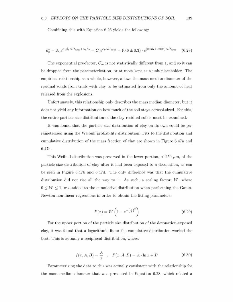
6.3. EFFECTS ON THE PARTICLE SIZE DISTRIBUTIONS OF SOIL 139
Combining this with Equation 6.26 yields the following:
d∗p = Aoeα1β1∆Hexpl+α1βo = Coe
c1∆Hexpl = (0.6± 0.3) · e(0.037±0.005)∆Hexpl (6.28)
The exponential pre-factor, Co, is not statistically different from 1, and so it can
be dropped from the parameterization, or at most kept as a unit placeholder. The
empirical relationship as a whole, however, allows the mass median diameter of the
residual solids from trials with clay to be estimated from only the amount of heat
released from the explosions.
Unfortunately, this relationship only describes the mass median diameter, but it
does not yield any information on how much of the soil stays aerosol-sized. For this,
the entire particle size distribution of the clay residual solids must be examined.
It was found that the particle size distribution of clay on its own could be pa-
rameterized using the Weibull probability distribution. Fits to the distribution and
cumulative distribution of the mass fraction of clay are shown in Figure 6.47a and
6.47c.
This Weibull distribution was preserved in the lower portion, < 250 µm, of the
particle size distribution of clay after it had been exposed to a detonation, as can
be seen in Figure 6.47b and 6.47d. The only difference was that the cumulative
distribution did not rise all the way to 1. As such, a scaling factor, W , where
0 ≤ W ≤ 1, was added to the cumulative distribution when performing the Gauss-
Newton non-linear regressions in order to obtain the fitting parameters.
F (x) = W
(1− e−( xλ)
k)
(6.29)
For the upper portion of the particle size distribution of the detonation-exposed
clay, it was found that a logarithmic fit to the cumulative distribution worked the
best. This is actually a reciprocal distribution, where:
f(x;A,B) =A
x; F (x;A,B) = A · lnx+B (6.30)
Parameterizing the data to this was actually consistent with the relationship for
the mass median diameter that was presented in Equation 6.28, which related a
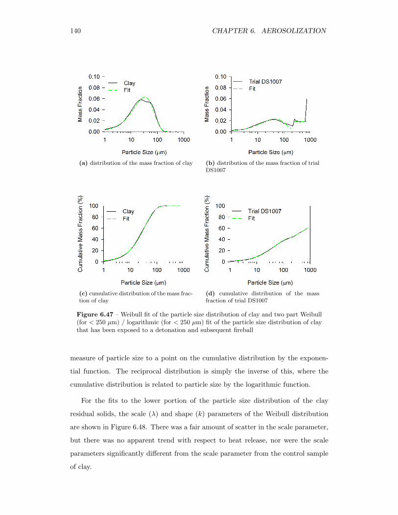
140 CHAPTER 6. AEROSOLIZATION
(a) distribution of the mass fraction of clay (b) distribution of the mass fraction of trialDS1007
(c) cumulative distribution of the mass frac-tion of clay
(d) cumulative distribution of the massfraction of trial DS1007
Figure 6.47 – Weibull fit of the particle size distribution of clay and two part Weibull(for < 250 µm) / logarithmic (for < 250 µm) fit of the particle size distribution of claythat has been exposed to a detonation and subsequent fireball
measure of particle size to a point on the cumulative distribution by the exponen-
tial function. The reciprocal distribution is simply the inverse of this, where the
cumulative distribution is related to particle size by the logarithmic function.
For the fits to the lower portion of the particle size distribution of the clay
residual solids, the scale (λ) and shape (k) parameters of the Weibull distribution
are shown in Figure 6.48. There was a fair amount of scatter in the scale parameter,
but there was no apparent trend with respect to heat release, nor were the scale
parameters significantly different from the scale parameter from the control sample
of clay.
6.3. EFFECTS ON THE PARTICLE SIZE DISTRIBUTIONS OF SOIL 141
(a) scale parameter (b) shape parameter
Figure 6.48 – Shape and scale parameters from Weibull fits to the < 250 µm fractionof the clay residual solids
The shape parameters, on the other hand, were all consistently less than the
shape parameter for the control sample of clay. However, the values were scattered
enough that there was no statistically significant difference between them. The 95%
confidence interval of the points (excluding the outlier) was (0.87, 1.14), and at 1.12,
the shape parameter of the control clay fell within this. One can say, therefore, that
although the distributions may be slightly more broad, the material in the < 250 µm
range was essentially unchanged from the control.
The distinct lack of trend in k and λ fit simply implied that the material in the
< 250 µ range was essentially just unreacted clay. In the fireball, however, it was
consumed to produce agglomerates, as shown by the strong linear decrease in the
scaling constant, W . The values of W are plotted in Figure 6.49, and such a high
correlation was felt to exist because W was a measure of the amount of material
remaining under 250 µm after a shot. The residual solids were bimodal, with the
unreacted clay on one side and the large agglomerates that were formed on the other.
A linear fit through the data points yielded:
W = β1 ·∆Hexpl + βo = (−0.0039± 0.0004) ·∆Hexpl + (1.13± 0.05) (6.31)
142 CHAPTER 6. AEROSOLIZATION
Figure 6.49 – Scaling constants from Weibull fits to the < 250 µm fraction of the clayresidual solids
Comparing this to Equation 6.26, it is clear that W = 1 − Faggl. Recognizing
that β1,W = −β1,aggl and βo,W = 1−βo,aggl, parameters from the two equation were
within the confidence intervals of each other.
The parameters for the logarithmic fit to the > 250 µm region are shown in
Figure 6.50. There was no clear trend in the log-intercept, B, but it was only
required to maintain continuity between the two fitting functions. The log-slope, A,
however, showed a clear linear trend where it decreased with fireball energy. This
implied that the reciprocal distribution became more broad, and particles spread out
into larger sizes as the clay was exposed to more and more heat from the fireball.
The linear fit to the log-slope parameter is as follows:
A = β1 ·∆Hexpl + βo = (−0.0011± 0.0003) ·∆Hexpl + (0.32± 0.06) (6.32)
With the information gained from the fits to the particle size distribution, an
empirical expression for the particle size distribution of clay residual solids could be
constructed. Recall first that an estimate for the agglomeration extent, Faggl, can
be calculated from the total heat released from the explosion using Equation 6.26:
6.3. EFFECTS ON THE PARTICLE SIZE DISTRIBUTIONS OF SOIL 143
(a) log-intercept (b) log-slope
Figure 6.50 – Shape and scale parameters from Weibull fits to the > 250 µm fractionof the clay residual solids
Faggl = β1 ·∆Hexpl + βo = (0.0043± 0.0005) ·∆Hexpl + (−0.22± 0.06) (6.33)
Faggl can then be used both in the pre-factor of the distribution in the < 250 µm
region, and to ensure continuity of the cumulative distribution in the > 250 µm
region. Recalling that k = 1 for the < 250 µm region simplifies the expressions as
well. In the end, the following can be used as the general parameterization for the
particle size distribution of the clay residual solids:
f(dp) =
(1− Faggl) ·
1
λe−
dpλ dp < 250 µm
A
dpdp ≥ 250 µm
(6.34a)
F (dp) =
(1− Faggl) ·
(1− e−
dpλ
)dp < 250 µm
A · ln(dp250
)+ (1− Faggl) dp ≥ 250 µm
(6.34b)
where A can be calculated using Equation 6.32, and λ = 36± 10 µm.
For the most part, the generalized parameterization offered fairly good predic-
tions of the particle size distributions of the clay residual solids. A plot of the
144 CHAPTER 6. AEROSOLIZATION
difference between the real and predicted cumulative mass fractions is shown in Fig-
ure 6.51. The residual plot from the outlier point was left out, as were the plots for
the trials carried out in low-oxygen, since the reciprocal distribution in the > 250 µm
region does not apply to them.
For the main set of trials, the difference between the real and predicted values
were generally less than 10%. The Weibull distribution was fairly sensitive to its
scale parameter, λ, and so errors associated with its variability were propagated to
produce a lot of the variability in Figure 6.51. Generally, though, the parameter-
ization that was developed and presented in Equation 6.34 remained close to the
measured particle size distributions.
Figure 6.51 – Residuals from fitting generalized parameterization to the cumulativedistributions of the clay residual solids
6.4 Dispersion of a Powdered Target Material
In the last section, it was shown that significant changes can occur to the particle
size distributions of soil when it becomes entrained in an explosive fireball. When
explosives disperse a hazardous powder, the particulates that are launched into
the air can interact with any entrained soil, and can influence the amount of the
hazardous material that remains aerosol-sized.
6.4. DISPERSION OF A POWDERED TARGET MATERIAL 145
In the last section, it was seen that a number of different mechanisms exist that
can affect entrained soil. In this section, the discussion will center on the particle
interactions, and specifically, on the interactions with soil that allow the dispersed
powders to become part of larger particles.
There are two main mechanisms through which these interactions can occur.
In the hot, turbulent fireball, the powder can either deposit onto the surfaces of
larger soil particulates, or can become incorporated into agglomerates as they form.
Examples of both of these can be seen in the micrograph in Figure 6.52, which
shows coarse sand after it had been exposed to a detonation of C-4 in an oxygenated
atmosphere. The bright spots in the micrograph were the lanthanum oxide particles,
and they can be seen incorporated throughout agglomerates, as well as deposited
onto the surfaces of larger, unbroken grains of sand.
SurfaceDepositionSurface
Deposition
AgglomerationAgglomeration
Figure 6.52 – Agglomeration and deposition of lanthanum oxide with coarse sand;agglomeration (blue) and surface deposition (red) highlighted with false colour
After being disseminated into the air by the initial detonation, the powder would
have become suspended in the hot product gases and would have circulated through-
out the closed vessel. In addition to the powder, any soil that was picked up by the
explosion would have been entrained in the fireball as well. The particles would
have come into contact with one another either because of the shear and velocity
gradients in the turbulent flow field, or because of inertial impaction whenever the
146 CHAPTER 6. AEROSOLIZATION
carrier gas changed direction. Since the particles had their own mass and inertia,
in the latter case, they would have deviated from the streamlines of the gas as it
circulated around. Larger particles would have been flung out faster from a circu-
lating flow, and would have impacted smaller particles that were in the path of their
trajectories.
The rate of change of the number of particles of a certain size (denoted by par-
ticle volume, v) is based on the rate at which they are produced through particle
interactions from smaller ones, and the rate at which they are consumed on interac-
tion with other particles to produce larger ones. This is described by the coagulation
equation (Friedlander, 2000):
∂
∂tn(v) =
1
2
∫ v
0β(v, v − v)n(v)n(v − v)dv −
∫ ∞0
β(v, v)n(v)n(v)dv (6.35)
where the 1/2 prefactor in the first term is because the integral counts each collision
twice. The collision frequency function, β(vi, vj), captures the mechanics involved
for colliding particles. In turbulent flow fields with particles > 1 µm, relationships
have been developed by Saffman and Turner (1956) that describe β(vi, vj) as a
function of the radii of the colliding particles, ai and aj , and turbulent energy, εd.
For turbulent shear, where particles travelling along one stream of gas collide
with particles in an adjacent stream, due to a velocity gradient, the collision fre-
quency can be described by:
β(vi, vj) = 1.3(ai + aj)3(εdν
)1/2(6.36)
where ν is the kinematic viscosity of the gas.
For inertial collisions in a turbulent flow field, where particles of different sizes
collide because they have different relaxation times, τ−1 = m/f , when they are in
an accelerating (i.e. circulating) flow, the collision frequency is:
β(vi, vj) = 5.7(ai + aj)2
∣∣∣∣ 1
τi− 1
τj
∣∣∣∣ ε3/4dν1/4(6.37)
For turbulent shear, interactions are purely geometrical, and depend on the rel-
ative size of the two particles involved. The collision frequency in this case increases
proportional to the cube of particle size, i.e. ∼ (ai + aj)3. With inertial impaction,
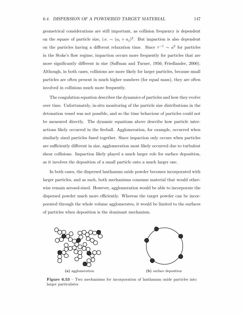
6.4. DISPERSION OF A POWDERED TARGET MATERIAL 147
geometrical considerations are still important, as collision frequency is dependent
on the square of particle size, i.e. ∼ (ai + aj)2. But impaction is also dependent
on the particles having a different relaxation time. Since τ−1 ∼ a2 for particles
in the Stoke’s flow regime, impaction occurs more frequently for particles that are
more significantly different in size (Saffman and Turner, 1956; Friedlander, 2000).
Although, in both cases, collisions are more likely for larger particles, because small
particles are often present in much higher numbers (for equal mass), they are often
involved in collisions much more frequently.
The coagulation equation describes the dynamics of particles and how they evolve
over time. Unfortunately, in-situ monitoring of the particle size distributions in the
detonation vessel was not possible, and so the time behaviour of particles could not
be measured directly. The dynamic equations above describe how particle inter-
actions likely occurred in the fireball. Agglomeration, for example, occurred when
similarly sized particles fused together. Since impaction only occurs when particles
are sufficiently different in size, agglomeration most likely occurred due to turbulent
shear collisions. Impaction likely played a much larger role for surface deposition,
as it involves the deposition of a small particle onto a much larger one.
In both cases, the dispersed lanthanum oxide powder becomes incorporated with
larger particles, and as such, both mechanisms consume material that would other-
wise remain aerosol-sized. However, agglomeration would be able to incorporate the
dispersed powder much more efficiently. Whereas the target powder can be incor-
porated through the whole volume agglomerates, it would be limited to the surfaces
of particles when deposition is the dominant mechanism.
(a) agglomeration (b) surface deposition
Figure 6.53 – Two mechanisms for incorporation of lanthanum oxide particles intolarger particulates
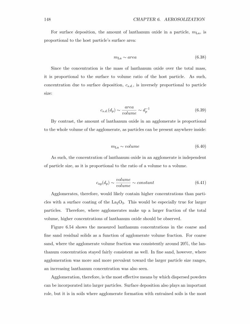
148 CHAPTER 6. AEROSOLIZATION
For surface deposition, the amount of lanthanum oxide in a particle, mLa, is
proportional to the host particle’s surface area:
mLa ∼ area (6.38)
Since the concentration is the mass of lanthanum oxide over the total mass,
it is proportional to the surface to volume ratio of the host particle. As such,
concentration due to surface deposition, cs.d., is inversely proportional to particle
size:
cs.d.(dp) ∼area
volume∼ d−1
p (6.39)
By contrast, the amount of lanthanum oxide in an agglomerate is proportional
to the whole volume of the agglomerate, as particles can be present anywhere inside:
mLa ∼ volume (6.40)
As such, the concentration of lanthanum oxide in an agglomerate is independent
of particle size, as it is proportional to the ratio of a volume to a volume.
cag(dp) ∼volume
volume∼ constant (6.41)
Agglomerates, therefore, would likely contain higher concentrations than parti-
cles with a surface coating of the La2O3. This would be especially true for larger
particles. Therefore, where agglomerates make up a larger fraction of the total
volume, higher concentrations of lanthanum oxide should be observed.
Figure 6.54 shows the measured lanthanum concentrations in the coarse and
fine sand residual solids as a function of agglomerate volume fraction. For coarse
sand, where the agglomerate volume fraction was consistently around 20%, the lan-
thanum concentration stayed fairly consistent as well. In fine sand, however, where
agglomeration was more and more prevalent toward the larger particle size ranges,
an increasing lanthanum concentration was also seen.
Agglomeration, therefore, is the most effective means by which dispersed powders
can be incorporated into larger particles. Surface deposition also plays an important
role, but it is in soils where agglomerate formation with entrained soils is the most
6.4. DISPERSION OF A POWDERED TARGET MATERIAL 149
Figure 6.54 – Correlation between lanthanum concentration and agglomeration extentin coarse sand and fine sand residual solids
prevalent that the most significant fraction of those powders would be removed from
the aerosol source term. This will be shown in the following sections, where it was
apparent that the lanthanum oxide tracer material became incorporated into large
particles in coarse sand, fine sand, and clay, but not in black earth because that soil
type was not subject to agglomeration in the fireball.
6.4.1 Coarse Sand
The cumulative mass distributions of lanthanum in the coarse sand residual solids
are shown as a function of particle size in Figure 6.55. For the shot carried out in
low-oxygen, a smaller amount of the lanthanum oxide was incorporated into larger
particles, and only about 36% of it was found in particles less than 50 µm. Particle
agglomeration is ultimately driven by turbulence, which is in turn driven by fireball
energy. Without that driving force, particle interactions would have been much less
frequent.
For the shot carried out in an oxygenated atmosphere, particles were able to
agglomerate with one another to a much greater extent, and more of the lanthanum
oxide powder was able to become incorporated into larger particles. Even less of
150 CHAPTER 6. AEROSOLIZATION
Figure 6.55 – Cumulative mass distribution of lanthanum, showing how it is dis-tributed throughout different sized particles in the coarse sand residual solids
the lanthanum (about 17%) remained among the aerosol-sized particles, as part of
material that was under 50 µm.
The average concentration of lanthanum in the residual solids, c, is basically the
total mass of lanthanum, MLa, in the soil over the total mass of soil, Msoil:
c =MLa
Msoil(6.42)
However, the concentration of lanthanum was not uniformly distributed through-
out the soil, with respect to particle size. The local concentration depends on the
ratio of lanthanum to residual solids at the specific particle size only. Given that
dM(dp) = M ·f(dp)d(dp), which relates the differential quantity of either lanthanum
or soil that has a particle size dp to the frequency function of their particle size dis-
tributions, the concentration of lanthanum, c(dp) in soil particles of a particular size
would be:
c(dp) =dMLa
dMsoil(6.43)
Expressed in terms of mass fraction, where dFm(dp) = fm(dp)d(dp):
6.4. DISPERSION OF A POWDERED TARGET MATERIAL 151
c(dp) = cdFLa
dFsoil(6.44)
Therefore, in a plot of the cumulative mass fraction of lanthanum, FLa(dp),
against the cumulative mass fraction of the residual soil, Fsoil(dp), the relative
concentration of lanthanum can be obtained from the slope of the curve. Where
dFLadFsoil
> 1, the concentration is above average, where when dFLadFsoil
< 1, the concen-
tration is below average.
This is seen in Figure 6.56, which shows the FLa-Fsoil plot for coarse sand. It can
be seen that the lanthanum was much more evenly distributed in the shot carried
out in an oxygenated atmosphere compared to the shot carried out in low-oxygen.
Without all the energy from the fireball to drive particle agglomeration, most of
the lanthanum was concentrated in the 0-44 µm and 44-53 µm ranges, while below
average concentrations were observed in the larger particle sizes. In the shot carried
out in an oxygenated atmosphere, on the other hand, the relative concentration at
small particle sizes was decreased while the relative concentration at large particle
sizes increased.
Figure 6.56 – Correlation between the cumulative mass distribution of lanthanum andthe total cumulative mass distribution of the coarse sand residual solids
152 CHAPTER 6. AEROSOLIZATION
6.4.2 Fine Sand
The cumulative mass distribution of lanthanum in the fine sand residual solids was
similar to that observed for coarse sand, as shown in Figure 6.57. Lanthanum
was more effectively distributed into larger particles when the shot was carried out
in an oxygenated atmosphere. Even though deposition of the lanthanum oxide
particles onto the surface of larger sand grains was still a significant effect, when
the detonation was carried out in low-oxygen, because there was no agglomeration,
the removal of lanthanum from the aerosol-sized fraction was not as effective. The
fraction of lanthanum in particles less than 50 µm was reduced to about 40% when
the shot was done in low-oxygen, but this was as low as 14% when the shot was
done in an oxygenated atmosphere.
The FLa-Fsoil plot for fine sand in Figure 6.58 shows that the highest La con-
centrations in the shot carried out in low-oxygen were in the 0-44 µm and 44-53 µm
ranges, with much lower relative concentrations (as seen by the shallower slopes)
elsewhere. For the shot carried out in an oxygenated atmosphere, on the other
hand, the highest lanthanum concentrations were seen at the highest particle sizes.
Figure 6.57 – Cumulative mass distribution of lanthanum, showing how it is dis-tributed throughout different sized particles in the fine sand residual solids
6.4. DISPERSION OF A POWDERED TARGET MATERIAL 153
Figure 6.58 – Correlation between the cumulative mass distribution of lanthanum andthe total cumulative mass distribution of the fine sand residual solids
The degree of agglomeration increases significantly with respect to particle size
for fine sand (recall Figure 6.13) to the point that residual solids are 100% agglom-
erates in the 600-841 µm and > 841 µm ranges. When agglomerate is common,
particles tend to have higher concentrations of the lanthanum oxide powder because
the smaller particulates would be incorporated through their whole volume, as op-
posed to single grains, where the powder can only be deposited onto their surfaces.
As the degree of agglomeration increases, there are fewer single grains, and the
overall concentration at that particle size increases.
6.4.3 Black Earth
With black earth, very little of the lanthanum oxide powder was incorporated into
larger particles. This can be seen in Figure 6.59, which shows that more than 95% of
the lanthanum remained as part of material that was less than 250 µm, while about
58% remained as part of aerosol-sized particles, below 50 µm. Moreover, there was
little change in the distribution of lanthanum between the shot that was carried out
in an oxygenated atmosphere versus the shot carried out in low-oxygen; the results
from the two shots were nearly identical.
154 CHAPTER 6. AEROSOLIZATION
Figure 6.59 – Cumulative mass distribution of lanthanum, showing how it is dis-tributed throughout different sized particles in the black earth residual solids
Likewise, the profiles for the two shots in the FLa-Fsoil plot in Figure 6.60 were
nearly the same. There was a slight decrease in the fraction of small particles in the
shot carried out in an oxygenated atmosphere because the carbonacous soot and
some of the smaller soil particulates were consumed in the fireball. This resulted
in a leftward shift of the two data points, corresponding to the 0-44 µm and 44-
53 µm ranges, while the overall slope (and therefore relative concentration) was
approximately the same. In any case, the slope was much higher in the smaller
particle size ranges, indicating that the lanthanum concentration was much greater.
On the other hand, the relative concentration in the large particle size ranges
was very low. This was because black earth particles, unlike those for sand and clay,
did not agglomerate in the fireball. Since the black earth particles were themselves
combustible, the fact that their surfaces were being eroded prevented them from
binding with other particles in the fireball. Without agglomeration, and to a large
extent without surface deposition as well, the lanthanum oxide powder did not
become incorporated into the larger particles, and as such mostly remained in the
aerosol-sized fraction.
6.4. DISPERSION OF A POWDERED TARGET MATERIAL 155
Figure 6.60 – Correlation between the cumulative mass distribution of lanthanum andthe total cumulative mass distribution of the black earth residual solids
6.4.4 Clay
With clay, particle agglomeration in the fireball was very dramatic. This has been
shown already in this chapter, and Figure 6.61 shows the effect this has on the
distribution of the lanthanum oxide powder through the clay. For the shot done in
low-oxygen, no agglomeration was observed. Although there was a slight reduction
in the quantity of lanthanum that remained aerosol-sized, as only 48% remained as
part of particles under 50 µm, over 96% of it remained as part of particles under
250 µm, meaning that there was really very little incorporation of it into large
particles.
However, for the shot done in an oxygenated atmosphere, the lanthanum became
incorporated into particles that were orders of magnitude larger than its original size.
Only about 25% of the material stayed as part of particles under 841 µm (the mesh
size of the largest screen in the mechanical sieve). More importantly, though, less
than 3% of the lanthanum remained as part of material less than 50 µm, meaning
that 97% of it was removed from the aerosol-sized fraction through interactions with
the clay that was entrained in the fireball.
156 CHAPTER 6. AEROSOLIZATION
Figure 6.61 – Cumulative mass distribution of lanthanum, showing how it is dis-tributed throughout different sized particles in the clay residual solids
Figure 6.62 shows the FLa-Fsoil plot for the residual clay. The slope was much
shallower at the larger particle sizes for the shot carried out in low-oxygen, which
indicates that the lanthanum concentration was much smaller than average at those
sizes. The concentration at small particle sizes, on the contrary, was much higher.
For the shot done in an oxygenated atmosphere, the lanthanum concentration was
lower for small particles, and higher for large particles. This was felt to be because
not all of the clay that was added to the vessel was entrained in the fireball. A
certain portion of it remained at the bottom of the vessel and did not form ag-
glomerates or interact with the lanthanum oxide powder. It is for this reason that a
lower slope (and therefore lanthanum concentration) was observed up until the point
corresponding to the cumulative mass fraction up to 250 µm. The only particles
above this size in the clay residual solids were agglomerates. The slope was fairly
constant above this point as well, meaning that the lanthanum concentration was
fairly constant, thus confirming the hypothesis that the concentration of a dispersed
powder remains constant throughout agglomerates, independent of their size.
6.5. SUMMARY 157
Figure 6.62 – Correlation between the cumulative mass distribution of lanthanum andthe total cumulative mass distribution of the clay residual solids
6.5 Summary
When particles are exposed to the high heat of the fireball, they can interact and fuse
together, with the result being an increase in the overall particle size and a reduction
of the quantity of particulates that are aerosol-sized. The experiments involving the
dispersion a powdered target clearly showed this: the formation of agglomerates in
the fireball and the resultant upward shift in the particle size distribution.
Entrained soil also interacted with the dispersed target, and underwent its own
physical changed when exposed to a detonation. Fracturing resulted in the genera-
tion of a small fragments, broken off from larger grains of coarse or fine sand. With
clay, agglomeration in the fireball produced dramatically large particles, and ag-
glomeration had a very noticeable effect in sand as well. In the latter cases, though,
an unidentified mechanism served to reduce particle size and counterbalanced the
effects of agglomeration. In black earth, however, agglomeration was inhibited be-
cause of particle combustion, which had its own influence on the overall particle size
distribution. The expressions that were developed to describe the size distribution
of the residual solids for each soil type are given in Tables 6.3-6.6.
158 CHAPTER 6. AEROSOLIZATION
Table 6.3 – Empirical expressions for coarse sand particle size distributions
Parameters
a = (4.8± 0.3)× 10−6 ·∆Hexpl[kJ ]− (6± 5)× 10−5 µm−1 (6.17)
d∗p =
490± 20 µm in low-oxygen
400± 50 µm in oxygenated atmosphere(6.15,6.16)
σ = 0.610± 0.006 (6.15,6.16)
Distributions
f(dp) =
a dp < 250 µm
1
dp√
2πσ2e−
(ln dp−ln d∗p)2
2σ2 dp ≥ 250 µm(6.18a)
F (dp) =
a · dp + b dp < 250 µm
1
2+
1
2erf
(ln dp − ln d∗p√
2σ2
)dp ≥ 250 µm
(6.18b)
Table 6.4 – Empirical expressions for fine sand particle size distributions
Parameters
λ = 240± 30 µm (6.19)k = 1.61± 0.01 (6.19)d∗p = 190± 20 µm
Distributions
f(dp) = kd∗p
ln 2 ·(dpd∗p
)k−1
· 2−(dpd∗p
)k(6.20)
F (dp) = 1− 2−(dpd∗p
)k(6.20)
Table 6.5 – Empirical expressions for black earth particle size distributions
Parameters
λ = (0.49± 0.09) ·∆Hexpl[kJ ] + (100± 10) µm (6.22)k = 0.974± 0.007
d∗p = (0.34± 0.06) ·∆Hexpl[kJ ] + (70± 9) µm (6.23)
Distributions
f(dp) = kd∗p
ln 2 ·(dpd∗p
)k−1
· 2−(dpd∗p
)k(6.25)
F (dp) = 1− 2−(dpd∗p
)k(6.25)
6.5. SUMMARY 159
Table 6.6 – Empirical expressions for clay particle size distributions
Parameters
λ = 36± 10 µmFaggl = (0.0043± 0.0005) ·∆Hexpl[kJ ] + (−0.22± 0.06) (6.33)A = (−0.0011± 0.0003) ·∆Hexpl[kJ ] + (0.32± 0.06) µm (6.32)
Distributions
f(dp) =
(1− Faggl) ·
1
λe−
dpλ dp < 250 µm
A
dpdp ≥ 250 µm
(6.34a)
F (dp) =
(1− Faggl) ·
(1− e−
dpλ
)dp < 250 µm
A · ln(dp250
)+ (1− Faggl) dp ≥ 250 µm
(6.34b)
Entrained soil added additional particles with which the dispersed target could
interact, but only when a mechanism existed that permitted the incorporation of
smaller particles into larger ones. For sand and clay, this occurs to a very significant
extent due to agglomeration and surface deposition. Since the combustion of black
earth in the fireball, however, inhibited the amalgamation of particles, entrainment
of black earth did not result in a change of the amount of the target that remained
aerosol-sized.
This chapter has shown that it is not sufficient to quantify the effects of explo-
sive aerosolization based on the initial detonation alone. In the fireball, there are
significant secondary effects, where interacting particles deposit onto one another,
or agglomerate together. The dispersed target material can become incorporated
into particles that would be too heavy to stay suspended in the atmosphere, and as
such, would be removed from the aerosol source term.

160 CHAPTER 6. AEROSOLIZATION
Chapter 7
Summary and Conclusions
7.1 Summary
Two sets of experiments were employed to study different aspects of fireball phe-
nomena and explosive aerosolization. Detonation calorimetry experiments involved
detonating small, 15 g charges of C-4 or detasheet inside a sealed detonation vessel.
Trials were carried out with explosives alone, as well as with four different types of
soil added to the bottom of the vessel. A small amount of lanthanum oxide powder
was used in a small subset of trials, and acted in the dual role as a surrogate haz-
ardous material, as well as a tracer to study particle agglomeration. In addition,
the quantity of oxygen in the vessel was varied in order to investigate what effects
energy release and fireball thermochemistry have on aerosolization.
The calorimeter measured the total heat release, and residual solids were sieved
into eight different particle size ranges. The particle morphology in each range was
measured using a scanning electron microscope, and particle size distributions were
measured using a Malvern Spraytec laser diffraction system. The distribution of
the lanthanum oxide powder throughout entrained soil was measured using neutron
activation analysis.
These experiments were complimented by a series of open air experiments em-
ployed to study fireball phenomena outside of the constrained environment of a
closed vessel. The open air trials employed a custom-built, fibre optic probe to
sample the thermal emissions from the interior of a fireball. The spectral composi-
tion of the emissions was characterized at two different sampling locations, and the
acquisition speed was high enough to resolve the evolution of the fireball over time.
161
162 CHAPTER 7. SUMMARY AND CONCLUSIONS
From the work that has been done, it has been found that there is a profound,
two-way relationship between the secondary fireball and the particles entrained in-
side. Not only does the fireball provide a sustained, high temperature, and turbulent
environment that drives particle interactions, but the combustion of particles is one
of the main mechanisms by which energy is released from the explosive fireball.
With respect to this latter point, thermochemical evidence that has been gath-
ered from the calorimetry measurements implies that the condensed phase detona-
tion products, e.g., carbonaceous soot, react much more quickly in the fireball than
gaseous species, e.g., CO, H2, CH4, NH3. The parallel reactions release different
amounts of heat per unit oxygen consumed, and from heat measurements obtained
at different initial oxygen partial pressures in the detonation vessel, it was found that
C(s) + 12O2 →CO reactions go essentially to completion before any of the reactions
involving gas phase species have a chance to proceed to any observable extent.
When soil entrainment effects with black earth were studied, due to its com-
bustion, less heat was evolved than when other types of soil were employed. The
addition of black earth meant that the system was overwhelmingly full of com-
bustible particulates, and because of this, about the same amount of heat release
per unit oxygen consumed was seen as for the reactions with the condensed phase
detonation products.
The likely reason for this is that the combustible particulates are able to mix
more efficiently with the air in the turbulent fireball, which in turn enhances the
rate at which they react compared to gaseous species. Particulates can deviate from
the streamlines of an accelerating (circulating) flow because the drag forces acting
upon them from the gas are not strong enough to keep them exactly in line with the
rest of the flow. Because of their inertia, particles can cross the interfaces between
mixing fluids, allowing them to come into greater contact with atmospheric oxygen.
The spectral measurements obtained during the open air trials found that the
thermal radiation at the interior of the fireball was predominantly from blackbody-
type emissions. This type of radiant spectrum is typical of fuel-rich combustion
flames, where the blackbody emissions come from tiny carbonaceous soot particu-
lates, and lack the emission lines that are more typical of leaner combustion and
primarily gas-gas reactions.
7.1. SUMMARY 163
The secondary fireball is the environment in which materials released from the
initial detonation are entrained. It is likely through the mechanisms of turbulent
shear and inertial impaction, driven by the turbulence in the fireball, that particles
can interact, and the high temperatures likely allow particles to fuse and sinter
together. This was observed among particles dispersed by the explosives, where for
the lanthanum oxide powder, the mass median diameter increased from about 23 µm
to about 45 µm.
Relating this to the aerosolization efficiency, as the overall size of particles in-
crease, it means that they are larger, heavier, and tend to fall out of the air at
much higher rates. Secondary effects in the fireball, therefore, reduce the quantity
of aerosols that would be released from an explosion. In addition, when certain
kinds of soil are entrained in the fireball, this reduction is even more dramatic. For
trials involving the dispersion of a powdered lanthanum oxide, only 17% and 14%
of the target remained in the fraction of material under 50 µm for coarse and fine
sand, respectively, while this was only 3% for clay. In the latter case, this meant
that because of particle interactions, 97% of the lanthanum oxide powder ended up
as part of material that would have been too large to stay suspended in the air as
aerosols.
This filtering effect due to soil entrainment, however, was not observed for all soil
types. For black earth, the lanthanum oxide powder did not become incorporated
into particles above 50 µm any more than what occurred naturally in the fireball
without the entrainment of soil. It was only through particle agglomeration and
surface deposition that the target powder could be incorporated into larger partic-
ulates, and this did not occur for black earth, since particle combustion inhibited
these other processes.
It is a fortuitous result, however, that when explosions are carried out over soil,
there are significant secondary effects in the fireball. Soil entrainment serves to
change the mix of particles in the cloud generated by an explosion, and in doing
so, gives hazardous materials sites with which to interact. It changes the fraction
of material that is small enough to stay suspended in the air as aerosols, and the
fraction of material that becomes too big and heavy, and settles out in the immediate
vicinity of the blast.

164 CHAPTER 7. SUMMARY AND CONCLUSIONS
Therefore, for the case where hazardous materials are maliciously disseminated
into the air through the use of explosives, the work carried out in this thesis will help
to better define the aerosol source term, help refine atmospheric dispersion models,
and ultimately help to give disaster planners and first responders additional tools
with which to mitigate the consequences of their release.
7.2 Recommendations and Future Work
The experiments were designed to cover a broad number of different conditions in
order to investigate as many phenomena as possible. It would be possible, though,
for a number of those phenomena to be studied in more depth in the future, and for
some of the limitations that were encountered in this work to be addressed.
For example, only 15 g explosive charges were employed, and although two trials
were carried out with only 30 g of coarse sand, the vast majority of trials involving
soil used 60 g at a time. Different effects may be observed if the soil-to-explosives
ratio were changed. Due to the mechanical limitations of the detonation vessel,
explosive charges larger than 15 g cannot be used, but more or less soil could be
added to the vessel, in particular to start to identify scaling effects.
It was difficult to fully characterize the manner in which the particle size dis-
tributions of coarse and fine sand shifted in the fireball, and more tests would be
required to fully resolve the particle size-vs-heat release curves. There must have
been an additional, unidentified mechanism that served to reduce the overall particle
size, counterbalancing the tendency for agglomeration to increase it, though finding
the cause of the unidentified effect was beyond the scope of this thesis.
X-ray diffraction, which could tell whether changes to the crystal structure of
the sand grains had occurred, could lead to an answer. An investigation of how ex-
posure to a blast and entrainment in a high temperature fireball affects the material
properties of soil, however, and using x-ray diffraction as the analytical technique,
could be a worthy study in its own right.
This type of study could also be carried out to investigate whether major changes
to the material properties of the target powder had occurred. Carrying out exper-
iments in a closed vessel proved to be a powerful approach because it kept all of
the dispersed material, soil, and other residual solids contained, without losses from
7.2. RECOMMENDATIONS AND FUTURE WORK 165
material being thrown clear of the blast zone. As such, a number of different target
materials, including, different powders, salts, ceramics, and metals, could be inves-
tigated. The closed vessel tests allow the full distribution of particle sizes to be
characterized, rather than only the fraction of material that was aerosolized as was
done in Harper et al. (2007); Wu et al. (2007); Andrews et al. (2009), and coupling
these with x-ray diffraction could provide further insight into the changes that occur
to the material properties for a range of different targets.
The dispersion of the powdered lanthanum oxide target was only employed for a
small number of trials, in part because the elemental composition analyses became
cost-prohibitive for the large number of samples that had to be processed. If the
experimental design and residual solids separations could be optimized, and a less
expensive analytical technique identified (possibly x-ray fluorescence or ICP-MS),
more trials could be carried out, and the evolution of target dispersion throughout
entrained soil could be more thoroughly investigated.
In addition, the environment inside the closed vessel could be characterized by
instrumenting it. As long as instrumentation could be installed without compro-
mising the integrity of the closed vessel, pressure and temperature sensors could
potentially be used. One of the drawbacks of this scheme is that complex reflections
off of the interior walls of the detonation vessel would preclude obtaining informa-
tion about the short-lived dynamics, but good measurements of the static pressures
and temperatures could nevertheless likely be achieved.
One of the shortcomings of the calorimetry measurements was that, based on the
initial partial pressures of oxygen at which the trials were carried out, the values of
the oxygen-weighted total reaction extent generally fell in the 0.4 ≤ χ ≤ 1.1 range.
It was difficult to carry out trials at higher initial oxygen partial pressures because
the plastic insulator in the high voltage terminal would melt and/or burn in the
fireball. However, by reducing the size of the explosive charge, another series of
trials could be done in order to confirm that above χ = 1, the heat release did reach
a plateau at η = 1. Trials should also be carried out so that more data points in the
0.0 < χ ≤ 0.4 range could be obtained. Other than the trials done in low-oxygen,
around χ = 0, there were no data points available to characterize the portion of the
η-χ relationship before the χcrit transition point.
166 CHAPTER 7. SUMMARY AND CONCLUSIONS
The conclusions made on the hierarchy of detonation product consumption in the
fireball were made on inferences from the heat release. These could have been greatly
supported, however, through measurements of the gas phase product compositions.
Although this was attempted, because of difficulties associated with gas sampling
and storage, as well as logistical problems in finding appropriate analytical facilities,
measurements were not obtained. By successfully obtaining these measurements in
the future, through a technique such as gas chromatography-mass spectroscopy, the
interpretations made in this thesis about fireball thermochemistry would be more
thoroughly substantiated.
Finally, a measure of how the results obtained during the detonation calorimetry
experiments scale to larger charge sizes, and apply to an uncontained environment,
would be very useful in extending this work’s applicability to real world situations.
Numerical simulations using a program like ANSYS AUTODYN could be employed,
and simulation results could be validated against the results obtained in this work,
and subsequently run for larger scale, unconfined situations.
It was important to couple the closed vessel experiments with open air tests, but
with only one probe, the thermal radiation from the interior of the fireball could
only be sampled from one point at a time. By either using multiple probes, or
by carrying out a larger number of trials at different sampling points, the spatial
distribution of blackbody temperature, optical density, emission lines (if observed),
etc., could be better characterized. In addition, it would be beneficial to conduct
future tests in an open (unconfined) space, as reflections of the blast wave off of the
walls of the semi-enclosed detonics bay resulted in translations to the location and
distortions to the shape of the fireball.
Better measurements of optical depth could be obtained by retrofitting the probe
with a laser optics system. By setting up a laser above the fiber optic sensor and
measuring (single wavelength) transmission, or by relying on backscatter from a laser
set up adjacent to the sensor, optical depth, and therefore particulate concentration,
could be obtained without having to rely on inference from signal intensity. By
employing two lasers, interferometry techniques could be used to measure particle
size and velocity as well, though by that point, the optics may start to become too
complex for use in a fiber optic probe for explosive fireball measurements.
7.2. RECOMMENDATIONS AND FUTURE WORK 167
Although emission peaks from the combustion of gas phase products were not
observed in any of the measured spectra, the only way to definitively confirm this
would be to replicate the tests with a broadband spectrometer that could obtain
data well into the infrared ranges. This would have to be done, though, with a fiber
optic cable with appropriate transmission characteristics and with a spectrometer
that would not sacrifice the high speed acquisition rate requirements. Sampling a
wider spectrum, however, would have the added benefit of improving temperature
estimates, as a greater portion of the blackbody curve could be obtained.
Even with the current fiber optic probe, the open air tests could be improved
through additional measurements of blast wave and spectral irradiance from the
exterior of the fireball. As energy is carried away from the explosion either as
mechanical blast energy, or through thermal radiation from the fireball, these mea-
surements would allow an energy balance to be performed, and the partitioning of
energy between the initial detonation and subsequent fireball to be calculated. From
the amount of energy emitted from the fireball, estimates for the afterburn reaction
extent could also be obtained, which would in turn help quantify the hierarchy of
detonation products consumption in an open air explosion, as well as the efficiency
of the overall secondary combustion phase.

168 CHAPTER 7. SUMMARY AND CONCLUSIONS
Bibliography
C. J. Anderson and P. D. Katsabanis, 2000. Evaluation of heats of detonation.Technical Report W7701-9-1483, Mining Resource Engineering Limited, Kingston,Ontario.
W. S. Andrews, E. J. Waller, P. Brousseau, G. Roy, X. Cao, K. A. M. Creber,and L. S. Erhardt, 2009. Use of stable isotopes as surrogates for radionuclidesfor security studies. Journal of Radioanalytical and Nuclear Chemistry, 282(3):919–922.
S. I. Ansimov and Y. B. Zeldovich, 1977. Rayleigh-Taylor instability of boundarybetween detonation products and gas in spherical explosion. Pis’ma v ZhurnalTekhnicheskoi Fiziki, 3:1081–1084.
D. P. Bacon and R. A. Sarma, 1991. Agglomeration of dust in convective cloudsinitialized by nuclear bursts. Atmospheric Environment, 25A(11):2627–2642.
K. Balakrishnan, F. Genin, D. V. Nance, and S. Menon, 2010. Numerical study ofblast characteristics from detonation of homogeneous explosives. Shock Waves,20(2):147–162.
H. L. Brode, 1959. Blast wave from a spherical charge. The Physics of Fluids, 2(2):217–229.
X. Cao, G. Roy, and W. S. Andrews, 2010. Modelling the concentration distributionsof aerosol puffs using artificial neural networks. Boundary-Layer Meteorology, 136(1):83–103.
X. Cao, W. J. Hurley, G. Roy, and W. S. Andrews, 2011a. Dispersion coefficientsfor gaussian puff models. Boundary-Layer Meteorology, 139(3):487–500.
X. Cao, G. Roy, P. Brousseau, L. S. Erhardt, and W. S. Andrews, 2011b. A cloud risemodel for dust and soot from high explosive detonations. Propellants, Explosives,Pyrotechnics, 36(4):303–309.
J. E. Cockayne, R. L. Edwards, W. L. Grove, and J. D. Knollenburg, 1987. Dustcloud diagnostics and characterization for the Minor Scale event. Technical ReportDNA-TR-87-210, SAIC, McLean, Virginia.
P. W. Cooper, 1996. Explosives Engineering. Wiley-VCH.
R. D. Cowan and W. Fickett, 1956. Calculation of the detonation properties of solidexplosives with the Kistiakowsky-Wilson equation of state. Journal of ChemicalPhysics, 24(5):932–939.
169
170 BIBLIOGRAPHY
CRTI, 2008. Project charter (CRTI-07-0103RD: Full-scale RDD experiments andmodels) to the memorandum of understanding concerning the chemical, biolgi-cal, radiological, nuclear or explosive research and technology initiative (CRTI).Technical report, DRDC Ottawa, Ottawa, Ontario.
J. M. Densmore, M. M. Biss, K. L. McNesby, and B. E. Homan, 2011. High-speeddigital color imaging pyrometry. Applied Optics, 50(17):2659–2665.
T. J. DeVito, X. Cao, G. Roy, J. R. Costa, and W. S. Andrews, 2009. Modellingaerosol concentration distributions from transient (puff) sources. Canadian Jour-nal of Civil Engineering, 36(5):911–922.
G. Dixon-Lewis, 1968. Flame stucture and flame reaction kinetics ii. Transportphenomena in multicomponent systems. Proceedings of the Royal Society A, 307:111–135.
A. Einstein, 1905. On the motion of small particles suspended in liquids at restrequired by the molecular-kinetic theory of heat. Annalen der Physik, 17:549–560.
Encyclopædia Britannica Online, 2012a. Humus. URL http://www.britannica.
com/EBchecked/topic/276408/humus. Accessed February 9, 2012.
Encyclopædia Britannica Online, 2012b. Humic acid. URL http://www.
britannica.com/EBchecked/topic/276207/humic-acid. Accessed February 9,2012.
Encyclopædia Britannica Online, 2012c. Fulvic acid. URL http://www.
britannica.com/EBchecked/topic/221974/fulvic-acid. Accessed February 9,2012.
L. S. Erhardt and S. Noel, 2009. Full-scale radiological dispersal devices experimentsand models. In Proceedings of the 2006 Public Security S & T Summer Symposium,June 15–18, pages 90–91, Ottawa, Ontario.
C. D. Ferguson and M. M. Smith, 2009. Assessing radiological weapons: Attackmethods and estimated effects. Defence Against Terrorism Review, 2(2):15–34.
L. Fried and P. Souers, 1994. CHEETAH: A next generation thermochemical code.Technical Report UCRL-ID-117240, Lawrence Livermoore National Laboratories,Livermoore, California.
S. K. Friedlander, 2000. Smoke, Dust, and Haze: Fundementals of Aerosol Dynam-ics. Oxford University Press, 2 edition.
S. K. Friedlander and C. S. Wang, 1966. The self-preserving particle size distributionfor coagulation by brownian motion. Journal of Colloid and Interface Science, 22(2):126–132.
D. L. Frost, Z. Zarei, and F. Zhang, 2005. Instability of combustion products inter-face from detonation of heterogeneous explosives. In International Colloquium onthe Dynamics of Explosions and Reactive Systems, July 31–August 5, Montreal,Quebec.
BIBLIOGRAPHY 171
J. M. Gordon, M. T. Spidell, J. Pitz, K. C. Gross, and G. P. Perram, 2010. Highspeed spectral measurements of IED detonation fireballs. In Proceedings of SPIE7665: Chemical, Biological, Radiological, Nuclear, and Explosives (CBRNE) Sens-ing XI, April 6, Orlando, Florida.
S. Goroshin, D. L. Frost, J. Levine, A. Yoshinaka, and F. Zhang, 2006. Optical py-rometry of fireballs of metalized explosives. Propellants, Explosives, Pyrotechnics,31(3):169–181.
F. T. Harper, S. V. Musolino, and W. B. Wente, 2007. Realistic radiological dispersaldevice hazard boundaries and ramifications for early consequence managementdecisions. Health Physics, 93(1):1–16.
W. C. Hinds, 1999. Aerosol Technology: Properties, Behavior, and Measurement ofAirborne Particles. Wiley-Interscience, 2 edition.
IAEA, 2007a. Arrangements for preparedness for a nuclear or radiological emergency.IAEA Safety Standard Series, No. GS-G-2.1, International Atomic Energy Agency.
IAEA, 2007b. Combating illicit trafficking in nuclear and other radioactive material.IAEA Nuclear Security Series, No. 6, International Atomic Energy Agency.
R. S. Jessup, 1948. The heat and free energy of polymerization of ethylene. Journalof Chemical Physics, 16(7):661–664.
P. D. Katsabanis, 1993. Development of a detonation calorimeter to measure the heatof detonation of high explosives. Technical report, Queen’s University, Kingston,Ontario.
R. Krasny, 1986. Desingularization of periodic vortex sheet roll-up. Journal ofComputational Physics, 65:292–313.
A. L. Kuhl, R. E. Ferguson, and A. K. Oppenheim, 1999. Gasdynamics of combus-tion of TNT products in air. Archivum Combustionis, 19(1–4):67–89.
L. S. Lebel, P. Brousseau, L. S. Erhardt, and W. S. Andrews, 2011. An investi-gation of aerosolization and associated phenomena resulting from the detonationof explosives. In Proceedings of the 26th International Symposium on Ballistics,September 12–16, pages 328–339, Miami, Florida.
L. S. Lebel, P. Brousseau, L. S. Erhardt, and W. S. Andrews, in press. Entrainmentof powders and soil into explosive fireballs. International Journal of EnergeticMaterials and Chemical Propulsion.
L. S. Lebel, P. Brousseau, L. S. Erhardt, and W. S. Andrews, submitted. Mea-surements of the temperature inside an explosive fireball. Journal of AppliedMechanics.
P. E. Liley, G. H. Thomson, D. G. Friend, T. E. Daubert, and E. Buck, 1997.Physical and Chemical Data. In R. H. Perry and D. W. Green, editors, Perry’sChemical Engineers’ Handbook, pages 2.195–2.198 and 2.306–2.307. McGraw Hill,7th edition.
172 BIBLIOGRAPHY
2006. Spraytec User Manual. Malvern Instruments Ltd., man0368 issue 2.0 edition.
F. A. Mettler and G. L. Voelz, 2002. Major radiation exposure - what to expect andhow to respond. New England Journal of Medicine, 346(20):1554–1561.
J. Mott Peuker, P. Lynch, H. Krier, and N. Glumac, 2009. Optical depth measure-ments of fireballs from aluminized high explosives. Optics and Lasers in Engi-neering, 47:1009–1015.
S. V. Musolino and F. T. Harper, 2006. Emergency response guidelines for thefirst 48 hours after the outdoor detontation of an explosive radiological dispersaldevice. Health Physics, 90(4):377–385.
OECD-NEA, 2002. CHERNOBYL: Assessment of radiological and health im-pacts 2002 update of Chernobyl: ten years on. Technical report, Organizationfor Economic Cooperation and Development: Nuclear Energy Agency, Issy-Les-Moulineaux, France.
D. L. Ornellas, 1982. Calorimetric determinations of heat and products of detona-tion for explosives: October 1961 to april 1982. Technical Report UCRL-52821,Lawrence Livermoore National Laboratory, Livermoore, California.
F. Pasquill, 1974. Atmospheric Diffusion. Ellis Horwood, 2 edition.
J. C. Russ, 2006. The Image Processing Handbook. CRC Press, 5 edition.
P. G. Saffman and J. S. Turner, 1956. On the collision of drops in turbulent clouds.Journal of Fluid Mechanics, 1:16–30.
D. Satas, 1989. Handbook of Pressure Sensitive Adhesives Technology. Van NostrandReinhold, 2nd edition.
R. Satgunanathan, 2007. Determining the particle size distributions of aerosolsgenerated from the breaking of ceramic pellets. Masters thesis, Royal MilitaryCollege of Canada.
M. Smoluchowski, 1916. Drei vortrage uber diffusion, brownsche bewegung undkoagulation von kolloidteilchen. Physikalische Zeitschrift, 17:557–585.
M. Smoluchowski, 1917. Drei vortrage uber diffusion, brownsche bewegung undkoagulation von kolloidteilchen. Zeitschrift fur Physikalische Chemie, 92:129–168.
M. T. Spidell, J. M. Gordon, J. Pitz, K. C. Gross, and G. P. Perram, 2010. Highspeed radiometric measurements of IED detonation fireballs. In Proceedings ofSPIE 7668: Airborne Intelligence, Surveillance, Reconnaissance (ISR) Systemsand Applications VII, April 7, Orlando, Florida.
G. I. Taylor, 1950. The instability of liquid surfaces when accelerated in a directionperpendicular to their planes. Proceedings of the Royal Society of London A:Mathematical and Physical Sciences, 201(1065):192–196.
S. R. Turns, 2006. An Introduction to Combustion. McGraw Hill, 2nd edition.
BIBLIOGRAPHY 173
A. E. Wildegger-Gaissmaier, 2003. Aspects of thermobaric weaponry. AustralianDefence Forces (ADF) Health, 4:3–6.
M. M. R. Williams and S. K. Loyalka, 1991. Aerosol science theory & practice: withspecial applications to the nuclear industry. Pergamon Press.
Q. Wu, K. M. Jaansalu, W. S. Andrews, L. S. Erhardt, G. Roy, and P. Brousseau,2007. Fracture and dispersion of selected ceramics under explosive loads. InProceedings of the 23rd International Symposium on Ballistics, April 16–20, pages1479–1486, Taragona, Spain.

174 BIBLIOGRAPHY
Appendix A
Table A.1 – List of shots carried out for detonation calorimetry experiments
DateShotCode
Explosive DetonatorPartial
Pressure N2
PartialPressure O2
Soil TypeLanthanum
Oxide
01/06/2010 C4060115.00 g
C-4RP-83 580 kPa 21 kPa None None
04/06/2010 DS060414.91 g
DetasheetRP-83 580 kPa 21 kPa None None
08/062010 C4060814.90 g
C-4RP-1 597 kPa 4 kPa None None
10/06/2010 DS061015.00 g
DetasheetRP-1 597 kPa 4 kPa None None
14/06/2010 C4061414.89 g
C-4RP-1 597 kPa 4 kPa None None
16/06/2010 R10616 None RP-1 597 kPa 4 kPa None None23/06/2010 R10623 None RP-1 597 kPa 4 kPa None None24/06/2010 R80624 None RP-83 597 kPa 4 kPa None None25/06/2010 R80625 None RP-83 597 kPa 4 kPa None None
29/06/2010 C4062914.88 g
C-4RP-83 642 kPa 4 kPa None None
30/06/2010 DS063014.40 g
DetasheetRP-83 601 kPa 4 kPa None None
28/07/2010 C4072814.94 g
C-4RP-83 642 kPa 4 kPa None None
27/07/2010 DS072914.78 g
DetasheetRP-83 642 kPa 4 kPa None None
03/08/2010 C4080314.90 g
C-4RP-83 511 kPa 135 kPa None None
05/08/2010 DS080514.87 g
DetasheetRP-83 516 kPa 137 kPa None None
10/08/2010 C4081014.95 g
C-4RP-83 516 kPa 137 kPa None None
12/08/2010 C4081214.95 g
C-4RP-83 527 kPa 140 kPa
30.55 gcoarse sand
None
17/08/2010 C4081714.95 g
C-4RP-83 522 kPa 138 kPa
60.40 gcoarse sand
None
19/08/2010 DS081914.88 g
DetasheetRP-83 522 kPa 138 kPa
60.72 gcoarse sand
None
24/08/2010 DS082414.98 g
DetasheetRP-83 516 kPa 137 kPa
60.72 gcoarse sand
None
26/08/2010 DS082614.95 g
DetasheetRP-83 642 kPa 4 kPa
60.72 gcoarse sand
None
30/08/2010 C4083014.96 g
C-4RP-83 642 kPa 4 kPa
59.24 gcoarse sand
None
175
176 APPENDIX A
Table A.1 (continued) – List of shots carried out for detonation calorimetry experi-ments
DateShotCode
Explosive DetonatorPartial
Pressure N2
PartialPressure O2
Soil TypeLanthanum
Oxide
31/08/2010 DS083114.93 g
DetasheetRP-83 522 kPa 138 kPa
63.14 gfine sand
None
07/09/2010 C40907 14.96 g -4 RP-83 522 kPa 138 kPa61.09 g
fine sandNone
09/09/2010 DS090914.93 g
DetasheetRP-83 642 kPa 4 kPa
60.70 gfine sand
None
14/09/2010 C4091414.88 g
C-4RP-83 642 kPa 4 kPa
59.49 gfine sand
None
16/09/2010 DS091614.89 g
DetasheetRP-83 522 kPa 138 kPa
59.06 gblack earth
None
21/09/2010 C4092114.88 g
C-4RP-83 511 kPa 135 kPa
60.07 gblack earth
None
23/09/2010 DS092314.78 g
DetasheetRP-83 649 kPa 4 kPa
62.03 gblack earth
None
28/09/2010 C4092814.96 g
C-4RP-83 649 kPa 4 kPa
65.15 gblack earth
None
30/09/2010 DS093014.86 g
DetasheetRP-83 522 kPa 138 kPa
64.40 gclay
None
05/10/2010 C4100514.95 g
C-4RP-83 522 kPa 138 kPa
61.05 gclay
None
07/10/2010 DS100714.92 g
DetasheetRP-83 522 kPa 138 kPa
62.32 gclay
None
12/10/2010 C4101214.90 g
C-4RP-83 663 kPa 4 kPa
59.42 gclay
None
14/10/2010 DS101414.99 g
DetasheetRP-83 649 kPa 4 kPa
63.54 gclay
None
19/10/2010 C4101914.92 g
C-4RP-83 516 kPa 98 kPa
62.36 gcoarse sand
None
21/10/2010 DS102114.68 g
DetasheetRP-83 541 kPa 98 kPa
60.29 gcoarse sand
None
26/10/2010 C4102614.97 g
C-4RP-83 510 kPa 97 kPa
63.57 gfine sand
None
27/10/2010 DS102714.79 g
DetasheetRP-83 528 kPa 98 kPa
61.52 gblack earth
None
02/11/2010 C4110214.70 g
C-4RP-83 510 kPa 94 kPa
62.33 gblack earth
None
04/11/2010 DS110414.93 g
DetasheetRP-83 489 kPa 91 kPa
59.63 gfine sand
None
08/11/2010 C4110814.96 g
C-4RP-83 523 kPa 95 kPa
60.38 gclay
None
10/11/2010 C4111014.89 g
C-4RP-83 514 kPa 97 kPa
61.76 gclay
None
16/11/2010 DS111614.91 g
DetasheetRP-83 521 kPa 97 kPa
60.57 gclay
None
18/11/2010 C4111814.87 g
C-4RP-83 556 kPa 69 kPa
59.99 gcoarse sand
None
23/11/2010 C4112314.92 g
C-4RP-83 550 kPa 68 kPa
61.57 gfine sand
None
25/11/2010 C4112514.93 g
C-4RP-83 570 kPa 70 kPa
58.78 gblack earth
None
07/12/2010 DS120714.74 g
DetasheetRP-83 409 kPa 223 kPa
65.59 gcoarse sand
None
177
Table A.1 (continued) – List of shots carried out for detonation calorimetry experi-ments
DateShotCode
Explosive DetonatorPartial
Pressure N2
PartialPressure O2
Soil TypeLanthanum
Oxide
09/12/2010 C4120914.97 g
C-4RP-83 550 kPa 68 kPa
62.70 gclay
None
13/12/2010 DS121314.60 g
DetasheetRP-83 364 kPa 254 kPa
59.14 gfine sand
None
14/12/2010 DS121414.76 g
DetasheetRP-83 392 kPa 205 kPa
67.47 gblack earth
None
15/12/2010 DS121514.80 g
DetasheetRP-83 397 kPa 215 kPa
60.21 gclay
None
02/04/2011 C4020414.85 g
C-4RP-83 649 kPa 4 kPa None 1.3484 g
02/07/2011 C4020714.71 g
C-4RP-83 642 kPa 4 kPa
60.32 gcoarse sand
1.2808 g
02/09/2011 C4020914.90 g
C-4RP-83 642 kPa 4 kPa
60.15 gfine sand
1.2717 g
02/11/2011 C4021114.78 g
C-4RP-83 635 kPa 4 kPa
59.93 gblack earth
1.3365 g
02/18/2011 C4021814.96 g
C-4RP-83 642 kPa 4 kPa
61.92 gclay
1.3243 g
02/28/2011 C4022814.88 g
C-4RP-83 522 kPa 138 kPa
62.13 gcoarse sand
1.3219 g
03/01/2011 C4030114.98 g
C-4RP-83 522 kPa 138 kPa
63.37 gfine sand
1.4147 g
03/02/2011 C4030214.84 g
C-4RP-83 532 kPa 141 kPa
60.00 gblack earth
1.3185 g
03/14/2011 C4031414.82 g
C-4RP-83 522 kPa 138 kPa
60.51clay
1.3268 g
03/16/2011 C4031614.69 g
C-4RP-83 527 kPa 140 kPa None 1.3273 g
03/22/2011 C4032214.92 g
C-4RP-83 527 kPa 140 kPa None 1.3056 g

178 APPENDIX A
Appendix B
(a) shot CAL0628, 0.99 g benzoic acid (b) shot CAL0705, 4.86 g benzoic acid
(c) shot CAL0707, 3.08 g benzoic acid (d) shot CAL0727, 2.07 g benzoic acid
Figure B.1 – Calorimetry measurements using benzoic acid for calibration
179
180 APPENDIX B
(a) shot R10616 (b) shot R10623
(c) shot R80624 (d) shot R80625
Figure B.2 – Calorimetry measurements to obtain heat contribution from detonators
(a) shot DS0604 (b) shot C40608
Figure B.3 – Calorimetry measurements during experimental program
181
(a) shot DS0610 (b) shot C40614
(c) shot C40629 (d) shot DS0630
(e) shot C40728 (f) shot DS0729
Figure B.3 (continued) – Calorimetry measurements during experimental program
182 APPENDIX B
(a) shot DS0805 (b) shot C40810
(c) shot C40812 (d) shot C40817
(e) shot DS0819 (f) shot DS0824
Figure B.3 (continued) – Calorimetry measurements during experimental program
183
(a) shot DS0826 (b) shot C40830
(c) shot DS0831 (d) shot C40907
(e) shot DS0909 (f) shot C40914
Figure B.3 (continued) – Calorimetry measurements during experimental program

184 APPENDIX B
(a) shot DS0916 (b) shot C40921
(c) shot DS0923 (d) shot C40928
(e) shot DS0930 (f) shot C41005
Figure B.3 (continued) – Calorimetry measurements during experimental program
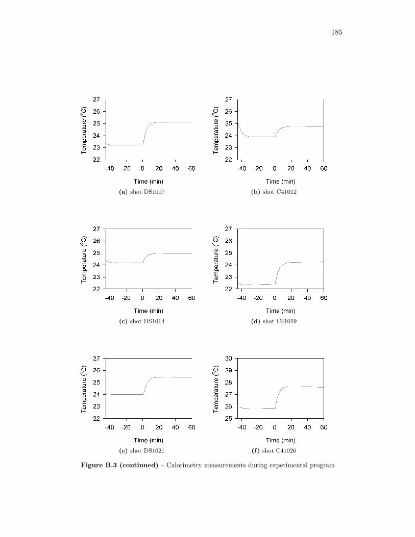
185
(a) shot DS1007 (b) shot C41012
(c) shot DS1014 (d) shot C41019
(e) shot DS1021 (f) shot C41026
Figure B.3 (continued) – Calorimetry measurements during experimental program
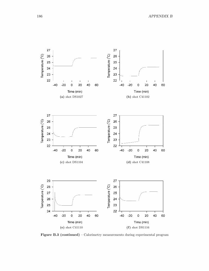
186 APPENDIX B
(a) shot DS1027 (b) shot C41102
(c) shot DS1104 (d) shot C41108
(e) shot C41110 (f) shot DS1116
Figure B.3 (continued) – Calorimetry measurements during experimental program
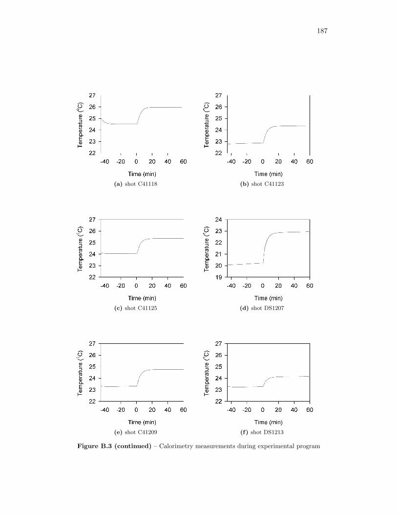
187
(a) shot C41118 (b) shot C41123
(c) shot C41125 (d) shot DS1207
(e) shot C41209 (f) shot DS1213
Figure B.3 (continued) – Calorimetry measurements during experimental program
188 APPENDIX B
(a) shot DS1214 (b) shot DS1215
(c) shot C40204 (d) shot C40207
(e) shot C40209 (f) shot C40218
Figure B.3 (continued) – Calorimetry measurements during experimental program

189
(a) shot C40228 (b) shot C40301
(c) shot C40302 (d) shot C40314
(e) shot C40316 (f) shot C40322
Figure B.3 (continued) – Calorimetry measurements with during experimental pro-gram

190 APPENDIX B
Appendix C
Table C.1 – Sieve analysis of control soils
Soil Type Mass (g) Collected on Screen with Mesh Size:841 µm 600 µm 420 µm 297 µm 250 µm 53 µm 47 µm pan
coarse sand 7.8749 12.5723 17.6157 18.6340 1.8085 2.4561 0.0117 0.0216fine sand 0.0912 0.0708 0.4009 7.9210 6.0115 47.9922 0.2776 0.1988
black earth 0.0963 0.0341 0.4179 6.1550 2.1853 31.4113 3.4052 19.1759clay 0.0000 0.0000 0.0000 0.0000 0.0000 5.5732 5.1792 46.3597
Table C.2 – Sieve analysis of residual solids from closed vessel trials
Shot Code Mass (g) Collected on Screen with Mesh Size:841 µm 600 µm 420 µm 297 µm 250 µm 53 µm 47 µm pan
C40601 5.1135 2.1472DS0604 1.7104 11.2362C40608 5.5156 0.3412DS0610 4.6616 3.0605C40614 4.6363 2.2093C40629 3.0309 2.5461DS0630 3.4554 3.3052C40728 1.0073 2.1419DS0729 1.4884 3.3287DS0805 1.0465 1.2775C40810 0.4582 2.0785C40812 3.3541 2.7384 4.6336 7.4583 1.6986 8.9818 0.2792 1.1244C40817 6.7269 6.7339 9.8677 13.3877 3.0106 17.8239 0.8430 3.9050DS0819 4.9993 7.5855 11.1541 15.6915 3.6777 17.0781 0.5513 2.4201DS0824 1.6284 2.0788 3.8911 7.7700 2.1053 12.6653 0.5144 2.3005DS0826 10.7633 12.9665 15.7137 14.8151 1.9576 6.0414 0.7286 3.1553C40830 10.8091 12.4642 13.0253 12.3308 2.0353 8.6456 0.5101 2.7890DS0831 0.9782 0.5744 1.1104 5.0288 4.0546 48.0504 1.4550 4.2701C40907 1.9515 0.9560 1.4639 5.3565 3.6327 42.5292 1.6980 5.6404DS0909 1.1476 0.3663 0.5302 4.8490 4.5357 48.2414 1.4878 4.5695C40914 0.8060 0.2875 0.5173 4.3532 3.7496 44.5184 1.7188 6.7704DS0916 5.7751 0.1884 0.8544 4.3281 3.2384 22.4753 2.3345 9.8537C40921 0.9909 0.2309 1.2710 4.9156 1.9754 24.4976 2.6297 12.9518DS0923 0.8221 0.3024 0.1540 3.7867 3.2847 28.8995 4.2442 18.9114C40928 1.5586 0.4440 0.5179 4.9410 3.9444 30.6557 5.0987 14.1015DS0930 10.5565 3.1344 3.9167 3.1183 1.4304 13.7261 3.8558 25.2815C41005 21.1601 3.2735 2.5523 2.4088 1.4769 17.9938 1.3084 10.5172DS1007 24.4929 2.5411 2.3670 1.9714 1.0417 14.7835 2.5230 12.7612C41012 1.7517 0.3811 0.6271 1.5885 2.3772 22.0689 5.5562 26.9986
191
192 APPENDIX C
Table C.2 (continued) – Sieve analysis of residual solids from closed vessel trials
Shot Code Mass (g) Collected on Screen with Mesh Size:841 µm 600 µm 420 µm 297 µm 250 µm 53 µm 47 µm pan
DS1014 2.0918 0.2855 0.3201 0.5773 0.4875 18.5360 4.7955 39.7585C41019 5.0198 7.5610 10.9737 12.2763 5.9372 18.2307 0.9798 3.5923DS1021 7.6280 9.6503 12.2731 12.6304 5.6602 12.5679 0.5012 1.8419C41026 0.5384 0.3545 0.4881 3.6959 6.9945 46.9818 1.7351 4.8658DS1027 0.7030 0.2514 0.6145 3.6347 3.1951 24.7737 2.7464 15.8483C41102 6.2641 0.2404 0.1892 4.6560 3.1188 22.8495 1.1435 13.6740DS1104 0.5295 0.2117 0.3375 3.2291 6.7401 44.2786 1.6018 4.9649C41108 24.1730 2.7412 2.8582 2.4300 1.2254 11.8107 1.5061 13.522C41110 25.1545 2.8741 2.6094 1.7037 1.1843 11.5836 2.0597 14.6055DS1116 10.4703 2.5596 2.5344 2.0303 1.3460 18.2949 3.3609 21.4751C41118 11.7790 12.3433 11.2481 8.6514 3.6268 12.3445 0.4709 1.7449C41123 0.5842 0.1562 0.3606 3.0035 6.3391 45.0745 2.2971 5.8466C41125 0.5744 0.1761 0.3304 3.4479 3.2826 23.1439 2.8005 15.6201DS1207 9.2650 10.3028 14.5159 13.4769 5.4448 11.7593 0.5659 2.4460C41209 9.6708 3.0732 3.6090 3.6316 2.6225 18.9464 2.3459 18.5026DS1213 0.8675 0.2375 0.0775 3.3720 6.7599 46.7010 1.3508 3.9754DS1214 1.4948 0.3924 0.5526 5.6419 4.1380 29.7187 2.9801 14.4062DS1215 29.6358 1.8755 1.1716 1.6870 0.6387 9.4910 2.0615 13.5602C40204 2.1310 4.0349C40207 11.6873 12.0461 11.6649 13.2612 4.0309 9.7070 1.0609 2.3528C40209 2.3354 0.4752 0.2445 4.3220 7.6122 43.5707 2.2884 5.1660C40211 1.5230 0.4331 0.1020 3.9720 3.1895 26.5021 6.3990 15.0891C40218 8.6287 0.7796 1.4585 2.4805 1.7663 28.8283 7.7744 14.1218C40228 6.3757 7.6482 10.0409 13.4579 5.8672 17.6497 0.8166 3.8055C40301 1.6560 1.1124 1.7454 5.3182 7.1345 3.3464 1.6749 5.1611C40302 8.3895 0.7394 1.3741 4.0580 2.5544 19.0514 1.9880 9.9300C40314 37.0051 2.2627 1.5889 2.2503 1.0612 9.5213 1.2712 7.2528C40316 0.7023 3.1302C40322 0.6236 2.9989
Appendix D
START
Setup and Calibration
Size / number ofparticles in
image?
Identify Particles(manual)
Identify Particles(auto)
Are thereagglomerates
present?
One phasemeasurements
Two phasemeasurements
FINISH
-save image as .psd file-create inverted duplicate layer-calibrate image w.r.t. scale bar-crop scale bar away
-preprocessing: smooth image-threshold grayscale to B&W-manually delineate and remove edge-touching particles
-threshold grayscale to B&W-erode+dilate to smooth edges-watershed segmentation to delineate particles-remove edge-touching particles
-measure features on B&W-create “background-free” grayscale image of particles
-manually identify agglomerates-create layers for separate types-measure features on B&W grain and agglomerate layers-create “background-free” grayscale image of two types of particles
many small particlesfew large particles
yesno
Figure D.1 – Flowchart of image processing steps using Fovea Pro plug-in for AdobePhotoshop
193

194 APPENDIX D
Action 1 – Setup and Calibration
1. save .tif image as .psd file
2. duplicate current layer
3. invert current layer
4. select top layer and invert:mask
5. merge selection
6. rename top layer: “Inverted Copy”
7. calibrate magnification (manually in pop-up window)
8. crop image (to remove scale bar)
9. levels: auto contrast
10. save
Action 2a – Identify Particles (manual)
1. duplicate “Inverted Copy” layer and name “Thresholded”
2. grayscale morphology, rank, 2 iterations
3. bilevel threshold (selecting appropriate algorithm in pop-up window)
4. EDM morphology, erode, 2 iterations
5. hide layer: “Inverted Copy”
6. set to 50% opacity layer: “Thresholded”
7. stop
8. manually delineate individual particle with brush tool, and erase edge-touchingparticles with paint bucket tool in layer: “Thresholded”
9. set to 100% opacity layer: “Thresholded”
10. show layer: “Inverted Copy”
11. bilevel threshold (selecting appropriate algorithm in pop-up window)
12. save
Action 2b – Identify Particles (auto)
1. duplicate “Inverted Copy” layer and name “Thresholded”
2. bilevel threshold (selecting appropriate algorithm in pop-up window)
3. EDM morphology, dilate, 1 iteration
4. EDM morphology, erode, 2 iterations
195
5. watershed segmentation
6. set to 35% opacity layer: “Thresholded”
7. stop
8. manually check results of segmentation
9. set to 100% opacity layer: “Thresholded”
10. reject features: edge cutoff
11. setup 2nd image to commit “Thresholded” layer image to memory
12. select history state: −2
13. boolean operation: AND
14. save
Action 3a – Two Phase Measurements
1. hide layer: “Inverted Copy”
2. hide layer: “Thresholded”
3. duplicate “Thresholded’ layer and name “Thresholded Agglomerates”
4. duplicate “Thresholded’ layer and name “Thresholded Grains”
5. show layer: “Thresholded Grains”
6. set to 50% opacity layer: “Thresholded Grains”
7. stop
8. manually erase any agglomerates particles using paint bucket tool in layer:“Thresholded Grains”
9. set to 100% opacity layer: “Thresholded Grains”
10. setup 2nd image to commit “Thresholded Grains” layer image to memory
11. hide layer: “Thresholded Grains”
12. show + select layer: “Thresholded Agglomerates”
13. boolean operation: Ex-OR
14. duplicate “Inverted Copy” layer and name “Inverted Grains”
15. duplicate “Inverted Copy” layer and name “Inverted Agglomerates”
16. show + select layer: “Inverted Grains”
17. keep lighter values between current layer and image in memory
18. hide layer: “Inverted Grains”

196 APPENDIX D
19. show + select layer: “Thresholded Agglomerates”
20. setup 2nd image to commit “Thresholded Agglomerates” layer image to mem-ory
21. show + select layer: “Inverted Agglomerates”
22. keep lighter values between current layer and image in memory
23. show + select layer: “Thresholded Grains”
24. measure all features, write to text file
25. show + select layer: “Thresholded Agglomerates”
26. measure all features, write to text file with append
27. show + select layer: “Thresholded”, hide all other layers above
28. label features
29. save
Action 3b – One Phase Measurements
1. show + select layer: “Thresholded”, hide all other layers above
2. setup 2nd image to commit “Thresholded” layer image to memory
3. hide layer: “Thresholded”
4. select layer: “Inverted Copy”
5. duplicate “Inverted Copy” layer and name “Inverted Particles”
6. keep lighter values between current layer and image in memory
7. measure all features, write to text file
8. show + select layer: “Thresholded”, hide all other layers above
9. label features
10. save
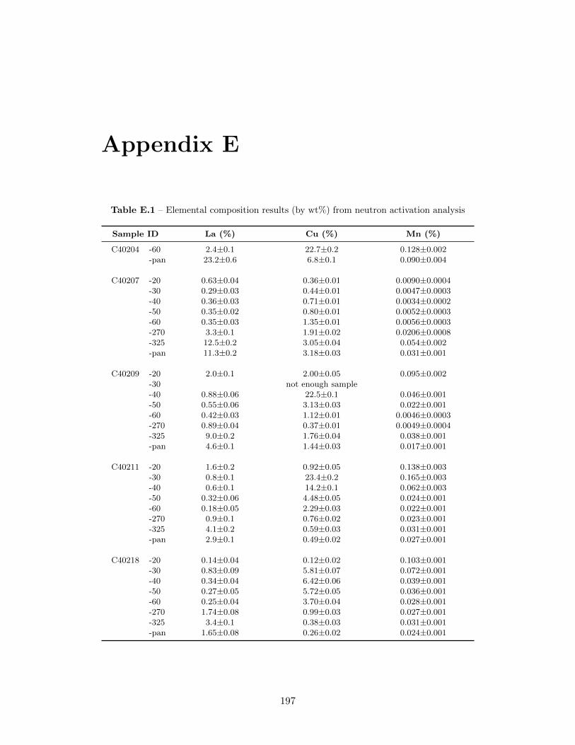
Appendix E
Table E.1 – Elemental composition results (by wt%) from neutron activation analysis
Sample ID La (%) Cu (%) Mn (%)
C40204 -60 2.4±0.1 22.7±0.2 0.128±0.002-pan 23.2±0.6 6.8±0.1 0.090±0.004
C40207 -20 0.63±0.04 0.36±0.01 0.0090±0.0004-30 0.29±0.03 0.44±0.01 0.0047±0.0003-40 0.36±0.03 0.71±0.01 0.0034±0.0002-50 0.35±0.02 0.80±0.01 0.0052±0.0003-60 0.35±0.03 1.35±0.01 0.0056±0.0003-270 3.3±0.1 1.91±0.02 0.0206±0.0008-325 12.5±0.2 3.05±0.04 0.054±0.002-pan 11.3±0.2 3.18±0.03 0.031±0.001
C40209 -20 2.0±0.1 2.00±0.05 0.095±0.002-30 not enough sample-40 0.88±0.06 22.5±0.1 0.046±0.001-50 0.55±0.06 3.13±0.03 0.022±0.001-60 0.42±0.03 1.12±0.01 0.0046±0.0003-270 0.89±0.04 0.37±0.01 0.0049±0.0004-325 9.0±0.2 1.76±0.04 0.038±0.001-pan 4.6±0.1 1.44±0.03 0.017±0.001
C40211 -20 1.6±0.2 0.92±0.05 0.138±0.003-30 0.8±0.1 23.4±0.2 0.165±0.003-40 0.6±0.1 14.2±0.1 0.062±0.003-50 0.32±0.06 4.48±0.05 0.024±0.001-60 0.18±0.05 2.29±0.03 0.022±0.001-270 0.9±0.1 0.76±0.02 0.023±0.001-325 4.1±0.2 0.59±0.03 0.031±0.001-pan 2.9±0.1 0.49±0.02 0.027±0.001
C40218 -20 0.14±0.04 0.12±0.02 0.103±0.001-30 0.83±0.09 5.81±0.07 0.072±0.001-40 0.34±0.04 6.42±0.06 0.039±0.001-50 0.27±0.05 5.72±0.05 0.036±0.001-60 0.25±0.04 3.70±0.04 0.028±0.001-270 1.74±0.08 0.99±0.03 0.027±0.001-325 3.4±0.1 0.38±0.03 0.031±0.001-pan 1.65±0.08 0.26±0.02 0.024±0.001
197
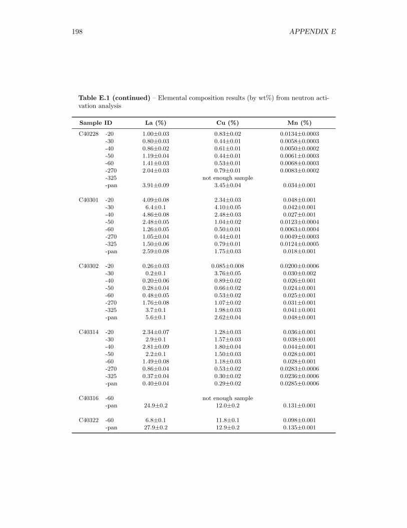
198 APPENDIX E
Table E.1 (continued) – Elemental composition results (by wt%) from neutron acti-vation analysis
Sample ID La (%) Cu (%) Mn (%)
C40228 -20 1.00±0.03 0.83±0.02 0.0134±0.0003-30 0.80±0.03 0.44±0.01 0.0058±0.0003-40 0.86±0.02 0.61±0.01 0.0050±0.0002-50 1.19±0.04 0.44±0.01 0.0061±0.0003-60 1.41±0.03 0.53±0.01 0.0068±0.0003-270 2.04±0.03 0.79±0.01 0.0083±0.0002-325 not enough sample-pan 3.91±0.09 3.45±0.04 0.034±0.001
C40301 -20 4.09±0.08 2.34±0.03 0.048±0.001-30 6.4±0.1 4.10±0.05 0.042±0.001-40 4.86±0.08 2.48±0.03 0.027±0.001-50 2.48±0.05 1.04±0.02 0.0123±0.0004-60 1.26±0.05 0.50±0.01 0.0063±0.0004-270 1.05±0.04 0.44±0.01 0.0049±0.0003-325 1.50±0.06 0.79±0.01 0.0124±0.0005-pan 2.59±0.08 1.75±0.03 0.018±0.001
C40302 -20 0.26±0.03 0.085±0.008 0.0200±0.0006-30 0.2±0.1 3.76±0.05 0.030±0.002-40 0.20±0.06 0.89±0.02 0.026±0.001-50 0.28±0.04 0.66±0.02 0.024±0.001-60 0.48±0.05 0.53±0.02 0.025±0.001-270 1.76±0.08 1.07±0.02 0.031±0.001-325 3.7±0.1 1.98±0.03 0.041±0.001-pan 5.6±0.1 2.62±0.04 0.048±0.001
C40314 -20 2.34±0.07 1.28±0.03 0.036±0.001-30 2.9±0.1 1.57±0.03 0.038±0.001-40 2.81±0.09 1.80±0.04 0.044±0.001-50 2.2±0.1 1.50±0.03 0.028±0.001-60 1.49±0.08 1.18±0.03 0.028±0.001-270 0.86±0.04 0.53±0.02 0.0283±0.0006-325 0.37±0.04 0.30±0.02 0.0236±0.0006-pan 0.40±0.04 0.29±0.02 0.0285±0.0006
C40316 -60 not enough sample-pan 24.9±0.2 12.0±0.2 0.131±0.001
C40322 -60 6.8±0.1 11.8±0.1 0.098±0.001-pan 27.9±0.2 12.9±0.2 0.135±0.001
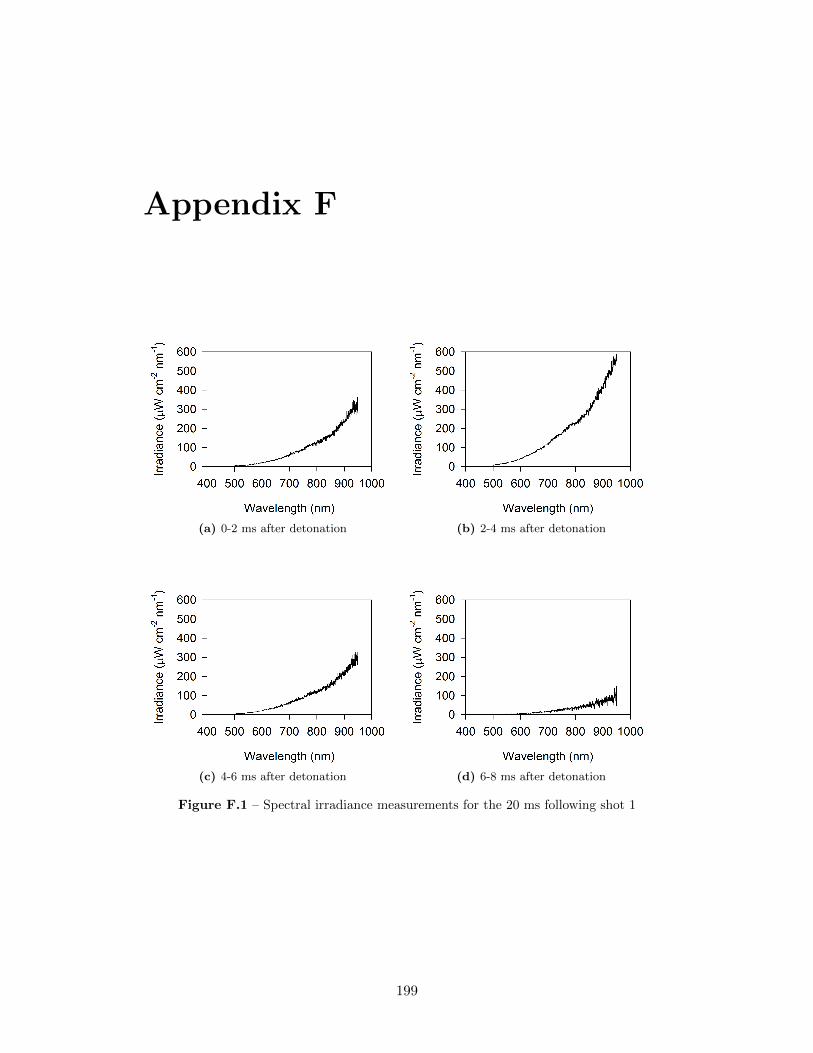
Appendix F
(a) 0-2 ms after detonation (b) 2-4 ms after detonation
(c) 4-6 ms after detonation (d) 6-8 ms after detonation
Figure F.1 – Spectral irradiance measurements for the 20 ms following shot 1
199
200 APPENDIX F
(a) 8-10 ms after detonation (b) 10-12 ms after detonation
(c) 12-14 ms after detonation (d) 14-16 ms after detonation
(e) 16-18 ms after detonation (f) 18-20 ms after detonation
Figure F.1 (continued) – Spectral irradiance measurements for the 20 ms followingshot 1
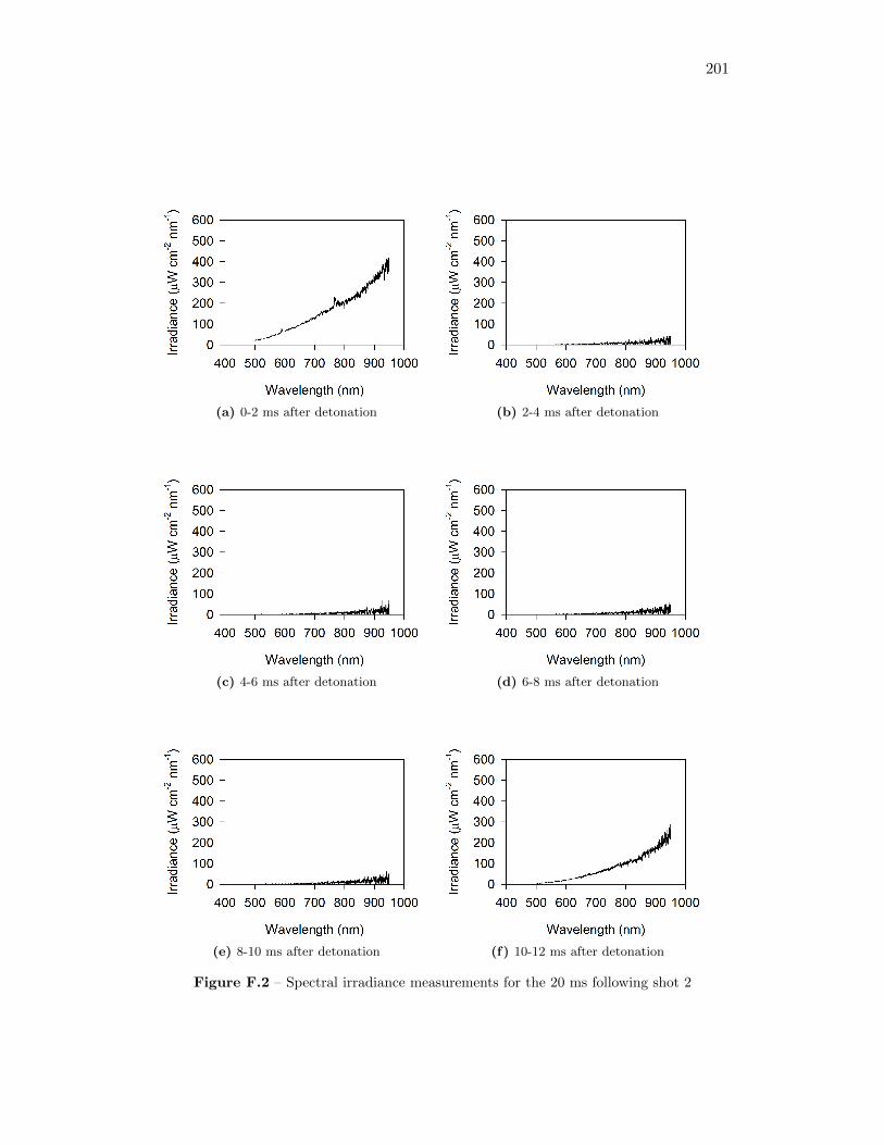
201
(a) 0-2 ms after detonation (b) 2-4 ms after detonation
(c) 4-6 ms after detonation (d) 6-8 ms after detonation
(e) 8-10 ms after detonation (f) 10-12 ms after detonation
Figure F.2 – Spectral irradiance measurements for the 20 ms following shot 2
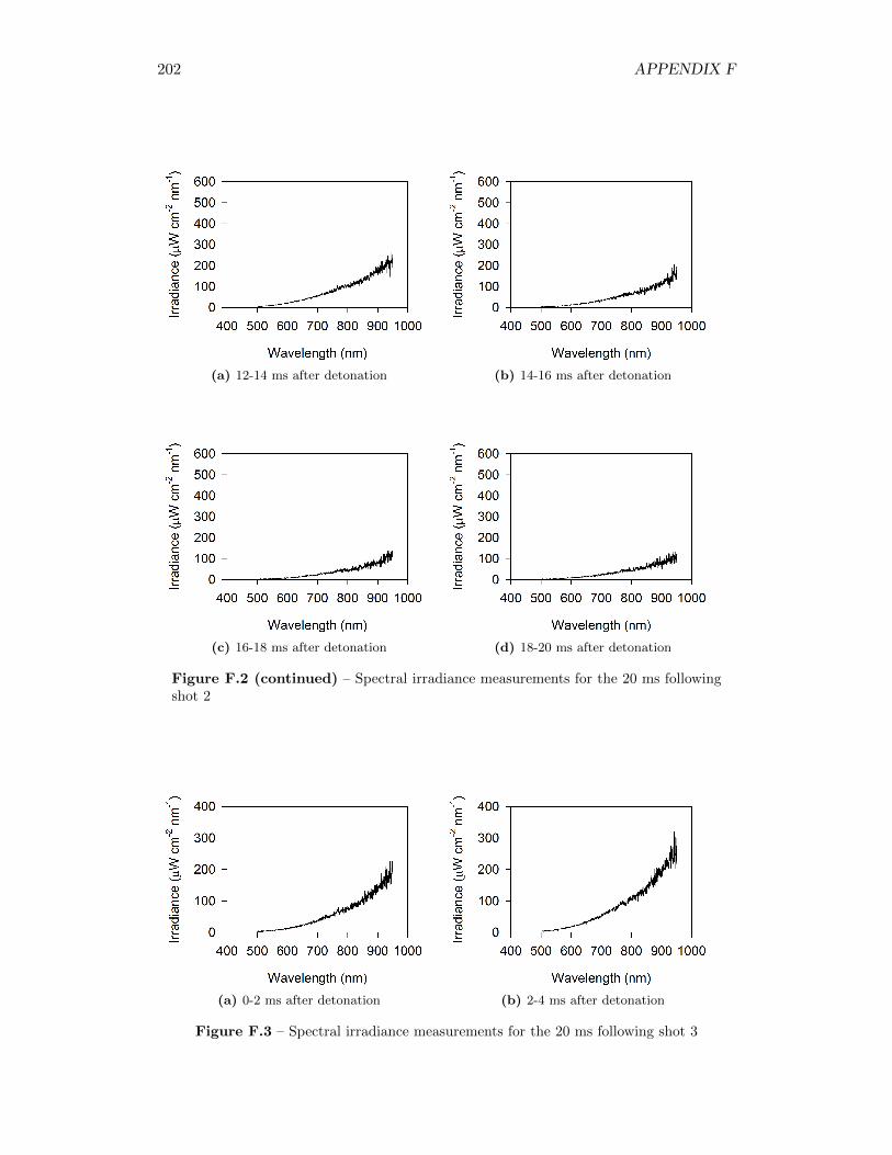
202 APPENDIX F
(a) 12-14 ms after detonation (b) 14-16 ms after detonation
(c) 16-18 ms after detonation (d) 18-20 ms after detonation
Figure F.2 (continued) – Spectral irradiance measurements for the 20 ms followingshot 2
(a) 0-2 ms after detonation (b) 2-4 ms after detonation
Figure F.3 – Spectral irradiance measurements for the 20 ms following shot 3
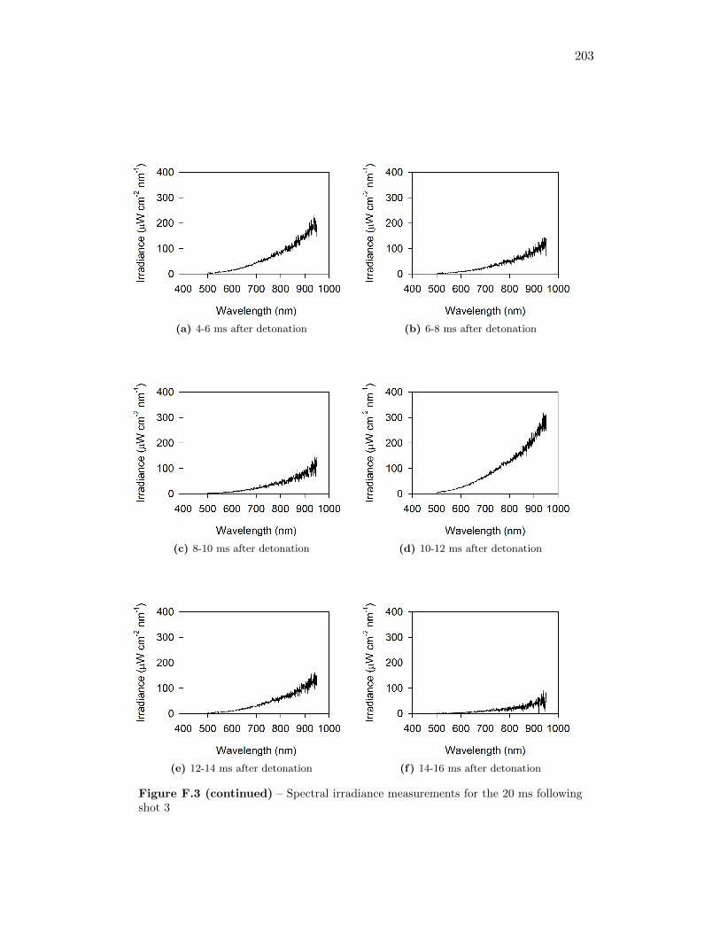
203
(a) 4-6 ms after detonation (b) 6-8 ms after detonation
(c) 8-10 ms after detonation (d) 10-12 ms after detonation
(e) 12-14 ms after detonation (f) 14-16 ms after detonation
Figure F.3 (continued) – Spectral irradiance measurements for the 20 ms followingshot 3
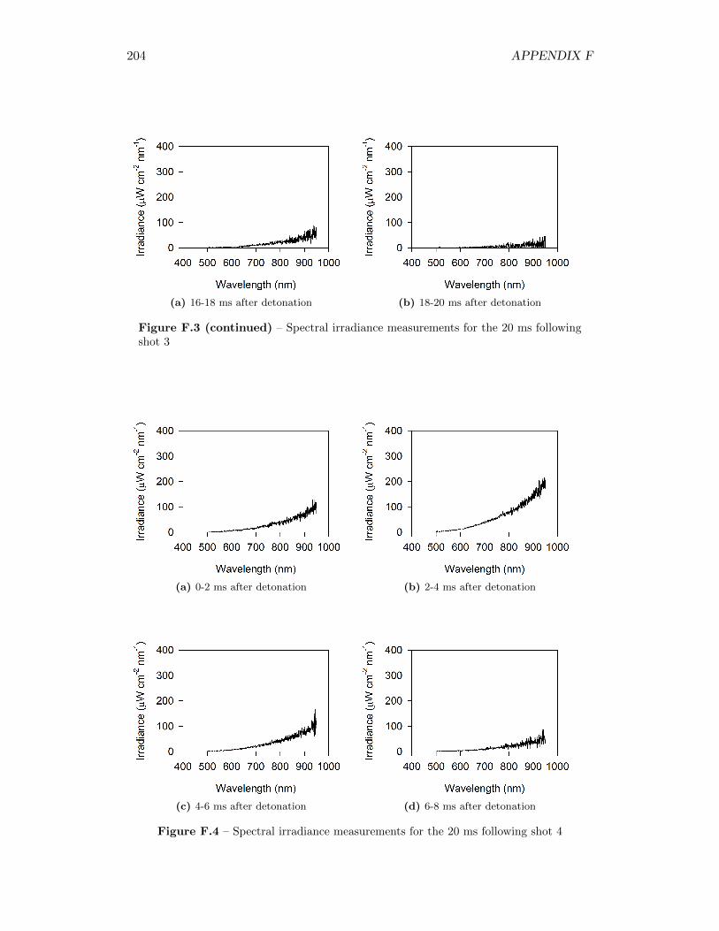
204 APPENDIX F
(a) 16-18 ms after detonation (b) 18-20 ms after detonation
Figure F.3 (continued) – Spectral irradiance measurements for the 20 ms followingshot 3
(a) 0-2 ms after detonation (b) 2-4 ms after detonation
(c) 4-6 ms after detonation (d) 6-8 ms after detonation
Figure F.4 – Spectral irradiance measurements for the 20 ms following shot 4
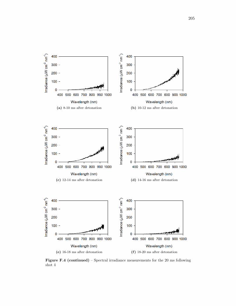
205
(a) 8-10 ms after detonation (b) 10-12 ms after detonation
(c) 12-14 ms after detonation (d) 14-16 ms after detonation
(e) 16-18 ms after detonation (f) 18-20 ms after detonation
Figure F.4 (continued) – Spectral irradiance measurements for the 20 ms followingshot 4
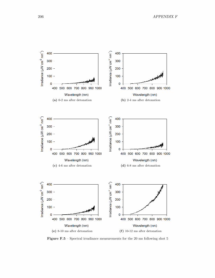
206 APPENDIX F
(a) 0-2 ms after detonation (b) 2-4 ms after detonation
(c) 4-6 ms after detonation (d) 6-8 ms after detonation
(e) 8-10 ms after detonation (f) 10-12 ms after detonation
Figure F.5 – Spectral irradiance measurements for the 20 ms following shot 5
207
(a) 12-14 ms after detonation (b) 14-16 ms after detonation
(c) 16-18 ms after detonation (d) 18-20 ms after detonation
Figure F.5 (continued) – Spectral irradiance measurements for the 20 ms followingshot 5

208 APPENDIX F
Appendix G
For Detasheet-C, the composition of species produced during the initial detonationcan be calculated using the CHEETAH thermochemical code (Fried and Souers,1994). Although the exact composition that is calculated depends of the equationof state that is employed, the BKWC equation of state is well validated for manycommon explosives. The heats of formation and number of moles of all speciesinvolved, given one mole of detasheet initially, and a stoichiometrically balancedcombustion in air, are tabulated below. Trace gases not tabulated contribute verylittle to overall heat release, and so were ignored.
Table G.1 – Heats of formation and composition for species involved in secondarycombustion reaction
SpeciesHeat of Formation
kJ·mol−1Initial Composition
(mol)Final Composition
(mol)
CO2 -394 3.09 8.68H2O -242 4.06 7.07
N2 expl. 0 1.37 1.46CO -111 0.58 –H2 0 0.69 –
CH4 -75 0.96 –NH3 -46 0.15 –C2H6 -75 0.04 –
CH2O2 -84 0.04 –C(s) -406 3.96 –
O2 0 6.80 –N2 air 0 25.34 25.34
Given that:
∆Hoab =
∑∆Ho
f (combustion products)−∑
∆Hof (detonation products)
the stoichiometric quantity of heat that would be released from the combustion ofthe detonation products produced from one mole of explosives would be ∆Ho
ab =3099 kJ.
The heat capacities of CO2, H2O(g), and N2 can be represented by polynomials,of the form tabulated by Liley et al. (1997):
cp,co2 [kJ ] = 4.33× 10⁻² + 1.15× 10⁻⁵T − 818T−2
cp,h2o[kJ ] = 3.44× 10⁻² + 6.28× 10⁻⁷T + 5.61× 10⁻⁹T 2
209
210 APPENDIX G
cp,n2 [kJ ] = 2.72× 10⁻² + 4.18× 10⁻⁶T
From Cooper (1996), the expression for the adiabatic flame temperature, assum-ing water in the vapour state, is:
∆Hab = n
∫ Ta
To
cpdT
The average heat capacity can be taken by weighting the individual heat capac-ities by the number of moles of each component. Taking the integral, subsequently,yields the following:
3099 = 1.34(Ta−To)+1.08×10⁻⁴(T 2a−T 2
o )+1.32×10⁻⁸(T 3a−T 3
o )+7.70×10³(T−1a −T−1
o )
Making the calculations for To = 298 K, this expression was solved numeri-cally using GoalSeek in Microsoft Excel to yield an estimate for the adiabatic flametemperature of T = 2152 K.

Curriculum Vitae
211

212 CURRICULUM VITAE

213
Curriculum Vitae
Luke Simon Lebel was born in Whitehorse, Yukon on January 3, 1986. Hecompleted his elementary and high school in Whitehorse, and was valedictorian forhis graduating class in 2004. He obtained his B.Sc. in Chemical Engineering fromQueen’s University, Kingston, Ontario in 2008, after which he enrolled in the NuclearEngineering graduate program at the Royal Military College of Canada.
EducationDoctor of Philosophy in Nuclear Engineering expected 2012
ROYAL MILITARY COLLEGE OF CANADA, Kingston, OntarioTHESIS: Aerosolization and Soil Entrainment in Explosive FireballsSUPERVISOR: Professor William Andrews
Bachelor of Science in Chemical Engineering 2008
QUEEN’S UNIVERSITY, Kingston, Ontario
Selected Honours and AwardsPost Graduate Scholarship – Doctoral, 2010
NATURAL SCIENCE AND ENGINEERING RESEARCH COUNCIL
Canada Graduate Scholarship – Masters, 2009
NATURAL SCIENCE AND ENGINEERING RESEARCH COUNCIL
University Medal in Chemical Engineering & E.T. Stern Prize 2008
QUEEN’S UNIVERSITY, convocation awards for highest academic standingover four years of study
ExperienceResearch Assistant (2008-present)
ROYAL MILITARY COLLEGE OF CANADA, Kingston, OntarioPROJECT: Experimental evaluation of explosive aerosolization, in-
cluding study of interactions with surrounding media (e.g.soil), in relation to dispersion of radiological material.
SUPERVISOR: Professor William Andrews
Research Assistant (2008)
QUEENS UNIVERSITY, Kingston, OntarioPROJECT: Twin-lift autonomous helicopter modeling and develop-
ment of mathematical framework for controller design.SUPERVISOR: Professor Martin Guay
Analytical Laboratory Technician (2007)
PROCTER AND GAMBLE LTD., Belleville, Ontario
214 CURRICULUM VITAE
SCOPE: Summer coop involving setup and management of newindustrial analytical laboratory, including qualification ofinstrumentation and training of personnel.
SUPERVISOR: Terrilynn Simpson
Engineering/Field Technician (2005, 2006)PROCTER AND GAMBLE LTD., Belleville, OntarioSCOPE: Groundwater monitoring around contaminated sites, in-
spection and analysis of drinking water supply systemsfrom groundwater.
SUPERVISOR: Ryan Martin
Publications and Presentations1 – L.S. Lebel, P. Brousseau, L. Erhardt, and W.S. Andrews, submitted. Mea-
surements of the temperature inside an explosive fireball. J. Appl. Mech.
2 – L.S. Lebel, P. Brousseau, L. Erhardt, and W.S. Andrews, in press. Entrain-ment of Powders and Soils Into Explosive Fireballs. Int. J. Energetic Mat. andChem. Prop.
3 – L.S. Lebel, P. Brousseau, L. Erhardt, and W.S. Andrews, 2012. Entrainmentof Powders and Soils Into Explosive Fireballs. Presented at the 9th InternationalSymposium on Special Topics in Chemical Propulsion, July 9-13, Quebec City,QC.
4 – L.S. Lebel, P. Brousseau, L. Erhardt, and W.S. Andrews, 2011. An Investi-gation of Aerosolization and Associated Phenomena Resulting From the Deto-nation of Explosives. In Proc. of the 26th International Ballistics Symposium,September 12-16, Miami, FL.
5 – L.S. Lebel, 2010. Licensing for detonation calorimetry experiments at theRoyal Military College of Canada. Presented at the DAER 4th Annual Ammu-nition and Explosives Safety Conference, November 29-December 2, GatineauQC.


![Types of Fireballs (Extended Version)giuliog/typesfire.pdf · 2018-10-29 · Types of Fireballs (Extended Version) 3 proof assistants, see Gr egoire and Leroy’s [29]. Typically,](https://img.dokumen.tips/doc/110x75/5f044daf7e708231d40d4fa1/types-of-fireballs-extended-version-giuliog-2018-10-29-types-of-fireballs.jpg)