1

A Maximizing Set and Minimizing Set Based Fuzzy

MCDM Approach for the Evaluation and Selection of

the Distribution Centers

Advisor:Prof. Chu, Ta-Chung

Student: Chen, Chun Chi

2

Outline

• Introduction

• Fuzzy set theory

• Model development

• Numerical example

• Conclusion

3

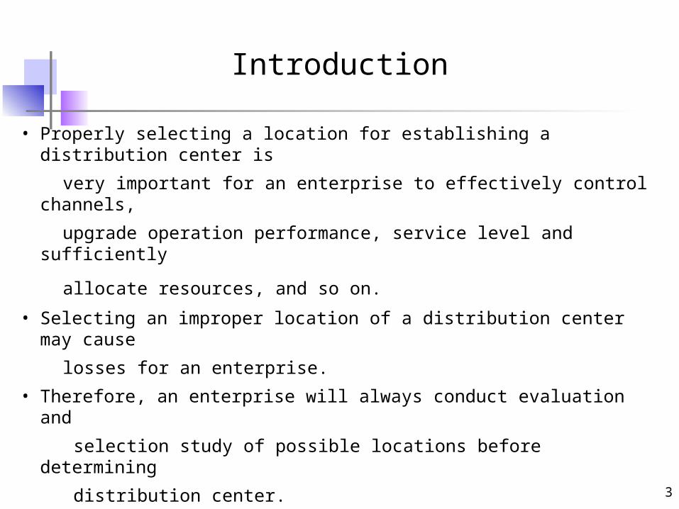
Introduction

• Properly selecting a location for establishing a distribution center is

very important for an enterprise to effectively control channels,

upgrade operation performance, service level and sufficiently

allocate resources, and so on. • Selecting an improper location of a distribution center may cause

losses for an enterprise.

• Therefore, an enterprise will always conduct evaluation and

selection study of possible locations before determining

distribution center.

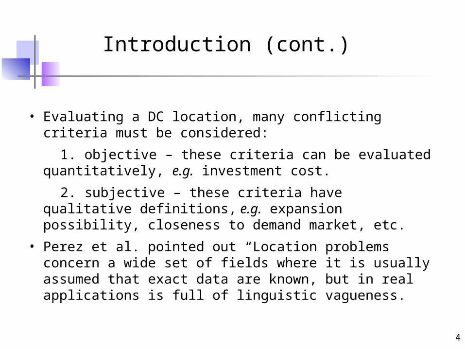
Introduction (cont.)

• Evaluating a DC location, many conflicting criteria must be considered:

1. objective – these criteria can be evaluated quantitatively, e.g. investment cost.

2. subjective – these criteria have qualitative definitions, e.g. expansion possibility, closeness to demand market, etc.

• Perez et al. pointed out “Location problems concern a wide set of fields where it is usually assumed that exact data are known, but in real applications is full of linguistic vagueness.

4

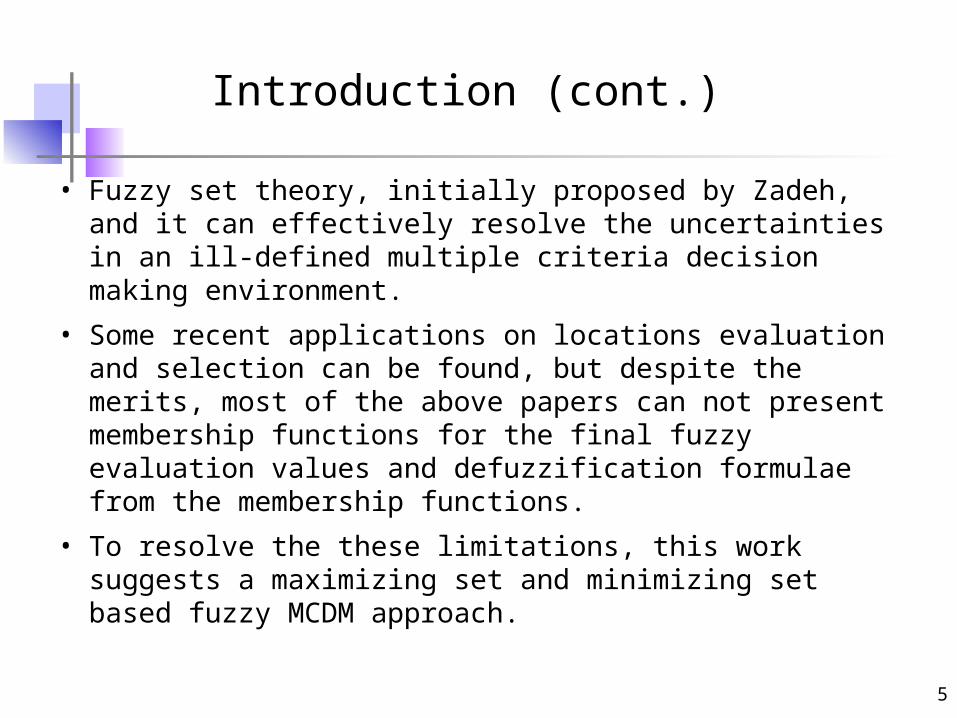
Introduction (cont.)

• Fuzzy set theory, initially proposed by Zadeh, and it can effectively resolve the uncertainties in an ill-defined multiple criteria decision making environment.

• Some recent applications on locations evaluation and selection can be found, but despite the merits, most of the above papers can not present membership functions for the final fuzzy evaluation values and defuzzification formulae from the membership functions.

• To resolve the these limitations, this work suggests a maximizing set and minimizing set based fuzzy MCDM approach.

5

6

Introduction (cont.)

Purposes of this paper:

• Develop a fuzzy MCDM model for the evaluation and selection of

the location of a distribution center.

• Apply maximizing set and minimizing set to the proposed model in

order to develop formulae for ranking procedure.

• Conduct a numerical example to demonstrate the feasibility of the

proposed model.

Fuzzy set theory

• 2.1 Fuzzy sets

• 2.2 Fuzzy numbers

• 2.3 α-cuts

• 2.4 Arithmetic operations on fuzzy numbers

• 2.5 Linguistic values

7

8

2.1 Fuzzy set

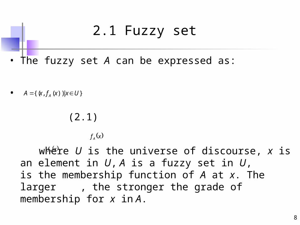
• The fuzzy set A can be expressed as:

• (2.1)

where U is the universe of discourse, x is an element in U, A is a fuzzy set in U, is the membership function of A at x. The larger , the stronger the grade of membership for x in A.

} |))( ,{( UxxfxA A

xf A

xf A

9

2.2 Fuzzy numbers

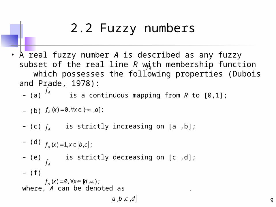
• A real fuzzy number A is described as any fuzzy subset of the real line R with membership function which possesses the following properties (Dubois and Prade, 1978):

– (a) is a continuous mapping from R to [0,1];

– (b)

– (c) is strictly increasing on [a ,b];

– (d)

– (e) is strictly decreasing on [c ,d];

– (f)

where, A can be denoted as .

Af

Af

; ] ,( ,0)( axxf A

Af

; , ,1)( cbxxf A

Af

; ) ,[ ,0)( dxxf A

dcba , , ,

10

2.2 Fuzzy numbers (Cont.)

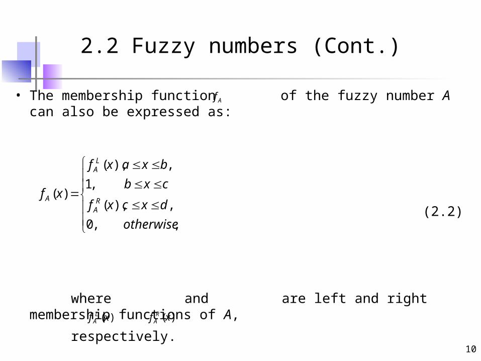
• The membership function of the fuzzy number A can also be expressed as:

(2.2)

where and are left and right membership functions of A,

respectively.

Af

, ,0

,),(

,1

,),(

)(

otherwise

dxcxf

cxb

bxaxf

xfR

A

LA

A

)(xf LA )(xf R

A

11

2.3 α-cut

• The α-cuts of fuzzy number A can be defined as:

(2.3)

where is a non-empty bounded closed interval contained in R and can be denoted by , where and are its lower and upper bounds, respectively.

1 ,0 , | xfxA A

A

] , [ ul AAA

lA uA

12

2.4 Arithmetic operations on fuzzy numbers

• Given fuzzy numbers A and B, , the α-cuts of A and B are

and respectively. By interval arithmetic, some main operations of A and B can be expressed as follows (Kaufmann and Gupta, 1991):

– (2.4)

– (2.5)

– (2.6)

– (2.7)

– (2.8)

RBA ,

] , [ ul AAA ], , [

ul BBB

] , [ uull BABABA

] , [ luul BABABA

] , [ uull BABABA

] , [ )(

l

u

u

l

B

A

B

ABA

RrrArArA ul , ,

13

2.5 Linguistic variable

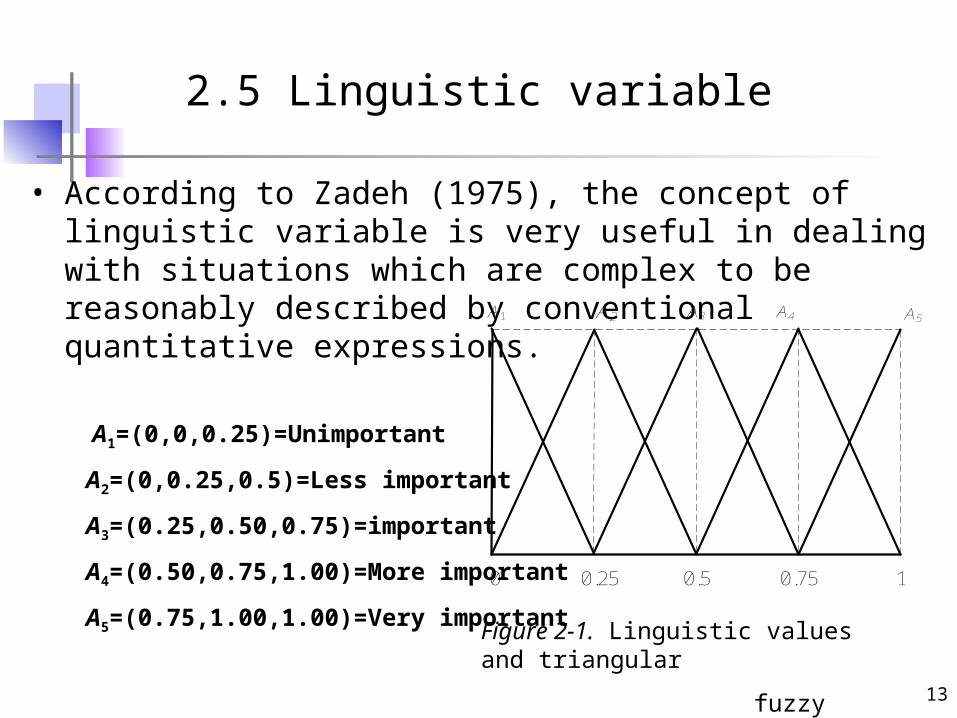
• According to Zadeh (1975), the concept of linguistic variable is very useful in dealing with situations which are complex to be reasonably described by conventional quantitative expressions.

A1=(0,0,0.25)=Unimportant

A2=(0,0.25,0.5)=Less important

A3=(0.25,0.50,0.75)=important

A4=(0.50,0.75,1.00)=More important

A5=(0.75,1.00,1.00)=Very important

Figure 2-1. Linguistic values and triangular

fuzzy numbers

0.50.250 0.75 1

A3 A5A4A2A1

14

Model development

• 3.1 Aggregate ratings of alternatives versus qualitative criteria

• 3.2 Normalize values of alternatives versus quantitative criteria

• 3.3 Average importance weights

• 3.4 Develop membership functions

• 3.5 Rank fuzzy numbers

15

Model development

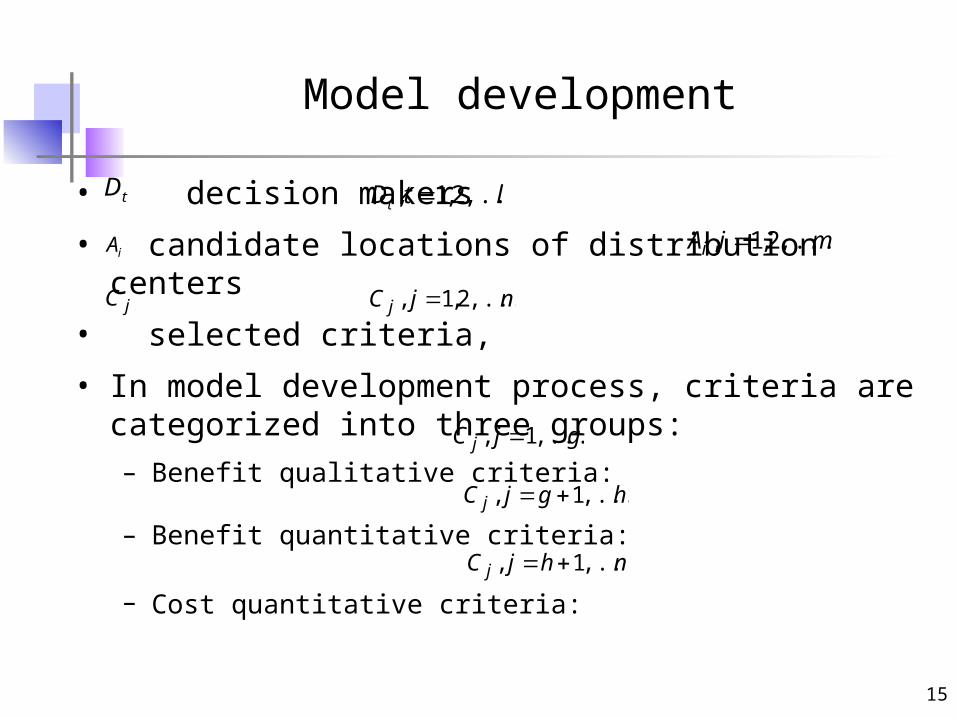
• decision makers

• candidate locations of distribution centers

• selected criteria,

• In model development process, criteria are categorized into three groups:

– Benefit qualitative criteria:

– Benefit quantitative criteria:

– Cost quantitative criteria:

ltDt ,...,2,1, tD

miAi ,...,2,1, iA

jC njC j ,...,2,1,

gjC j ,...,1,

hgjC j ,...,1,

nhjC j ,...,1,

16

3.1 Aggregate ratings of alternatives versus

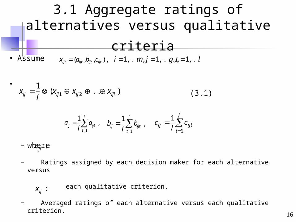
qualitative criteria • Assume

• (3.1)

– where

– Ratings assigned by each decision maker for each alternative versus

each qualitative criterion.

– Averaged ratings of each alternative versus each qualitative criterion.

, ),,( ijtijtijtijt cbax ltgjmi ,...,1,,...,1,,...,1

)...(1

21 ijlijijij xxxl

x

, 1

1

l

tijtij a

la ,

1

1

l

tijtij b

lb

l

tijtij c

lc

1

1

:ijtx

:ijx

17

3.2Normalize values of alternatives versus quantitative criteria

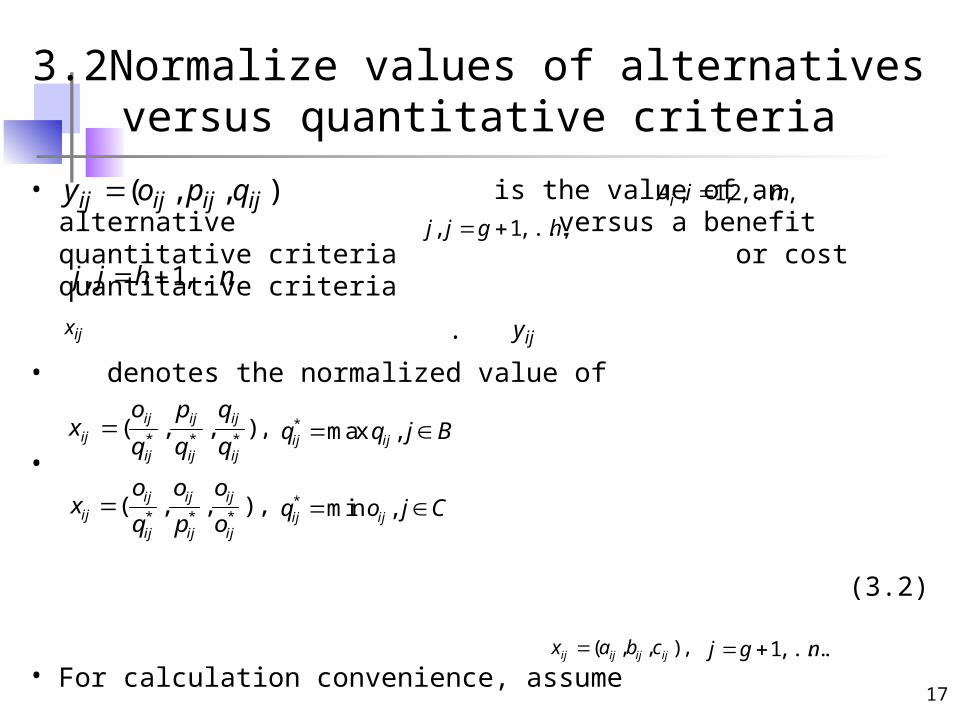
• is the value of an alternative versus a benefit quantitative criteria or cost quantitative criteria

.

• denotes the normalized value of

•

(3.2)

• For calculation convenience, assume

),,( ijijijij qpoy ,,...,2,1, miAi

,,...,1, hgjj

nhjj ,...,1,

ijx ijy

, ),,(***ij

ij

ij

ij

ij

ijij q

q

q

p

q

ox * max ,ij ijq q j B

, ),,( ijijijij cbax . ,...,1 ngj

* * *( , , ) ,ij ij ij

ijij ij ij

o o ox

q p o * min ,ij ijq o j C

18

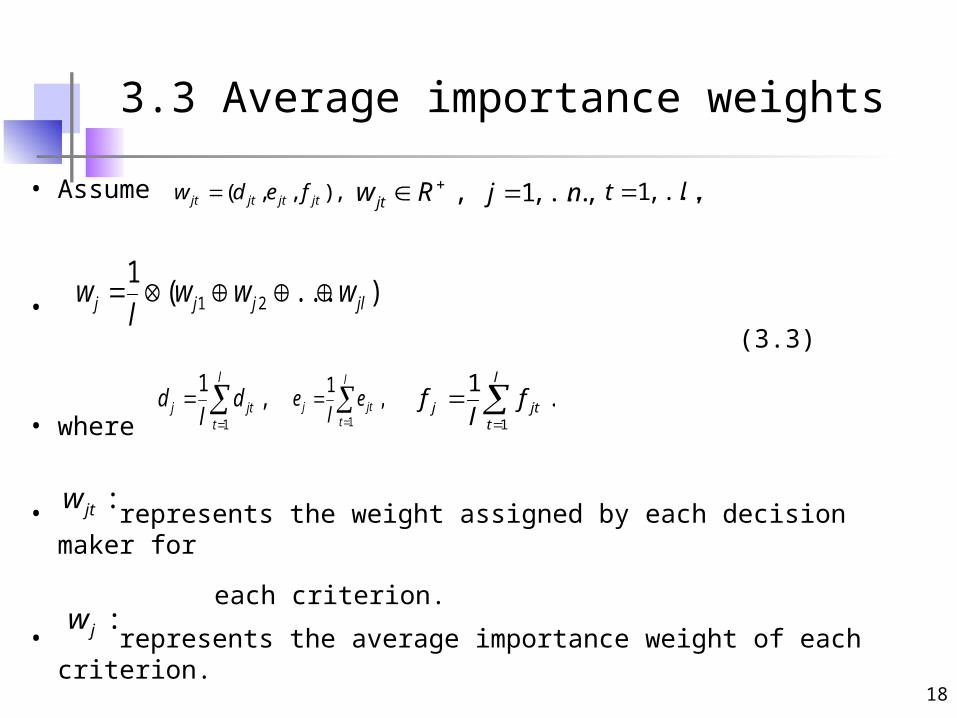
3.3 Average importance weights

• Assume

• (3.3)

• where

• represents the weight assigned by each decision maker for

each criterion. • represents the average importance weight of each criterion.

, ),,( jtjtjtjt fedw , Rw jt , ,...,1 nj , ,...,1 lt

)...(1

21 jljjj wwwl

w

, 1

1

l

tjtj d

ld ,

1

1

l

tjtj e

le .

1

1

l

tjtj f

lf

:jtw

:jw

19

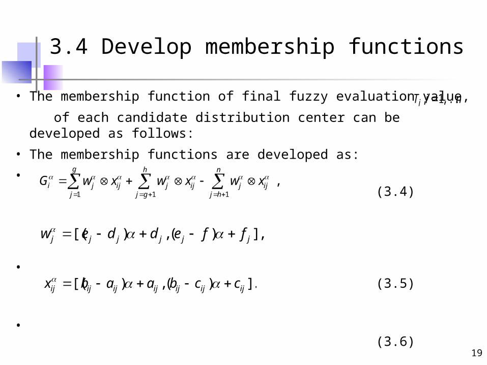
3.4 Develop membership functions

• The membership function of final fuzzy evaluation value,

of each candidate distribution center can be developed as follows:

• The membership functions are developed as:

• (3.4)

• (3.5)

• (3.6)

niTi ,...,1,

1 1 1

,g h n

i j ij j ij j ijj j g j h

G w x w x w x

, ])(,)[( jjjjjj ffeddew

. ])(,)[( ijijijijijijij ccbaabx

20

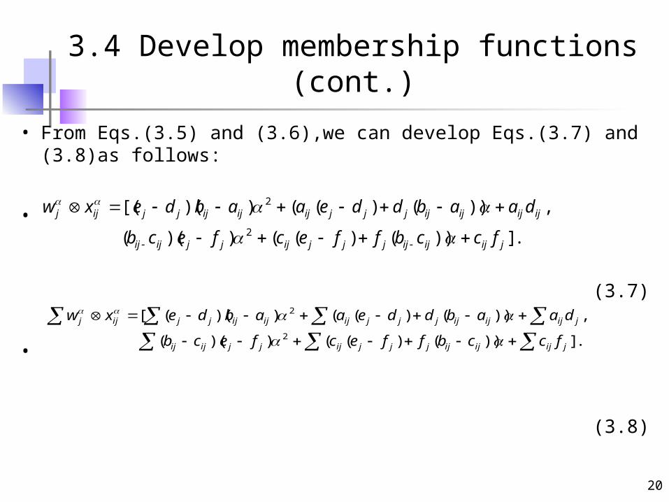
3.4 Develop membership functions (cont.)

• From Eqs.(3.5) and (3.6),we can develop Eqs.(3.7) and (3.8)as follows:

•

(3.7)

•

(3.8)

. ]))()(())((

,))()(())([(2

2

jijijijjjjijjjijij

ijijijijjjjijijijjjijj

fccbffecfecb

daabddeaabdexw

. ]))()(())((

,))()(())(([2

2

jijijijjjjijjjijij

jijijijjjjijijijjjijj

fccbffecfecb

daabddeaabdexw

21

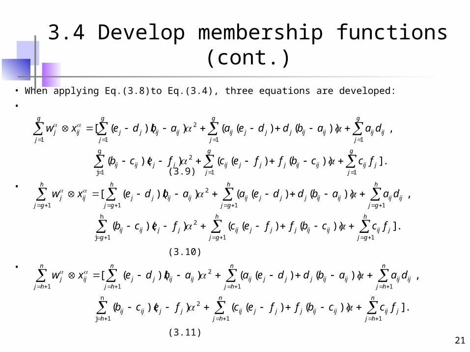
3.4 Develop membership functions (cont.)

• When applying Eq.(3.8)to Eq.(3.4), three equations are developed:

•

(3.9)

•

(3.10)

•

(3.11)

g

1j 1 1

2

11 1 1

2

. ]))()(())((

, ))()(())(([

g

j

g

jjijijijjjjijjjijij

g

jijij

g

j

g

j

g

jijijjjjijijijjjijj

fccbffecfecb

daabddeaabdexw

h

1j 1 1

2

11 1 1

2

. ]))()(())((

, ))()(())(([

g

h

gj

h

gjjijijijjjjijjjijij

h

gjijij

h

gj

h

gj

h

gjijijjjjijijijjjijj

fccbffecfecb

daabddeaabdexw

n

1j 1 1

2

11 1 1

2

. ]))()(())((

, ))()(())(([

h

n

hj

n

hjjijijijjjjijjjijij

n

hjijij

n

hj

n

hj

n

hjijijjjjijijijjjijj

fccbffecfecb

daabddeaabdexw

22

k

hjjiji

h

gjjiji

g

jjiji

k

hjjiji

h

gjjiji

g

jjiji

k

hjjiji

h

gjjiji

g

jjiji

k

hjijijjjjiji

h

gjijijjjjiji

g

jijijjjjiji

k

hjjjijiji

h

gjjjijiji

g

jjjijiji

k

hjijijjjjiji

h

gjijijjjjiji

g

jijijjjjiji

k

hjijijjji

h

gjijijjji

g

jijijjji

fcQ

fcQfcQ

ebPebP

ebPdaO

daOdaO

cbffecDcbffecD

cbffecDfecbC

fecbCfecbC

abddeaBabddeaB

abddeaBabdeA

abdeAabdeA

13

12

11

13

12

11

13

12

11

13

12

11

13

12

11

13

12

11

13

12

11

)()( )()(

))((

))(( ))((

))((

))(( ))((

:Assume

23

3.4 Develop membership functions (cont.)

• By applying the above equations, Eqs.(3.9)-(3.11) can be arranged as Eqs.(3.12)-(3.14)as follows:

• (3.12)

• (3.13)

• (3.14)

. ],[ 112

1112

11

iiiiiiij

g

jj QDCOBAxw

. ],[ 222

2222

21

iiiiiiij

h

gjj QDCOBAxw

. ],[ 332

3332

31

iiiiiiij

n

hjj QDCOBAxw

24

3.4 Develop membership functions (cont.)

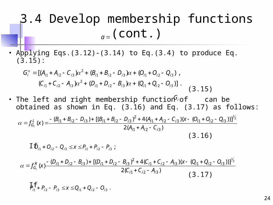
• Applying Eqs.(3.12)-(3.14) to Eq.(3.4) to produce Eq.(3.15):

(3.15)

• The left and right membership function of can be obtained as shown in Eq. (3.16) and Eq. (3.17) as follows:

(3.16)

If

(3.17)

If

iG

21 2 3 1 2 3 1 2 3

21 2 3 1 2 3 1 2 3

[( ) ( ) ( ) ,

( ) ( ) ( )] .

i i i i i i i i i i

i i i i i i i i i

G A A C B B D O O Q

C C A D D B Q Q O

; 321321 iiiiii PPPxQOO

. 321321 iiiiii OQQxPPP

a

122

1 2 3 1 2 3 1 2 3 1 2 3

1 2 3

( ) [( ) 4( )( ( ))]( )

2( )i

L i i i i i i i i i i i iG

i i i

B B D B B D A A C x O O Qf x

A A C

122

1 2 3 1 2 3 1 2 3 1 2 3

1 2 3

( ) [( ) 4( )( ( ))]( )

2( )i

R i i i i i i i i i i i iG

i i i

D D B D D B C C A x Q Q Of x

C C A

25

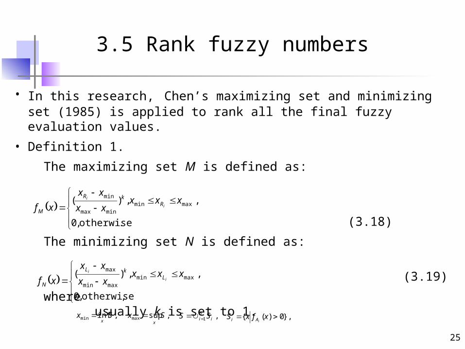
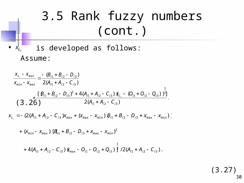
3.5 Rank fuzzy numbers

• In this research, Chen’s maximizing set and minimizing set (1985) is applied to rank all the final fuzzy evaluation values.

• Definition 1.

The maximizing set M is defined as:

(3.18)

The minimizing set N is defined as:

(3.19)

where usually k is set to 1.

. otherwise,0

, ,)( maxminminmax

min xxxxx

xx

xf i

i

RkR

M

, otherwise,0

, ,)( maxminmaxmin

maxxxx

xx

xx

xf i

i

LkL

N

, infmin Sxx

, supmax Sxx

, 1 ini SS , }0)({ xfxS

iAi

26

3.5 Rank fuzzy numbers (cont.)

Definition 2.

The right utility of is defined as:

(3.20)

The left utility of is defined as:

(3.21)

The total utility of is defined as:

(3.22)

iA

iA

. ~1, ))()((sup)( nixfxfAUiAM

xiM

. ~1, ))()((sup)( nixfxfAUiAM

xiN

iA

. ~1, ))(1)((2

1)( niAUAUAU iNiMiT

27

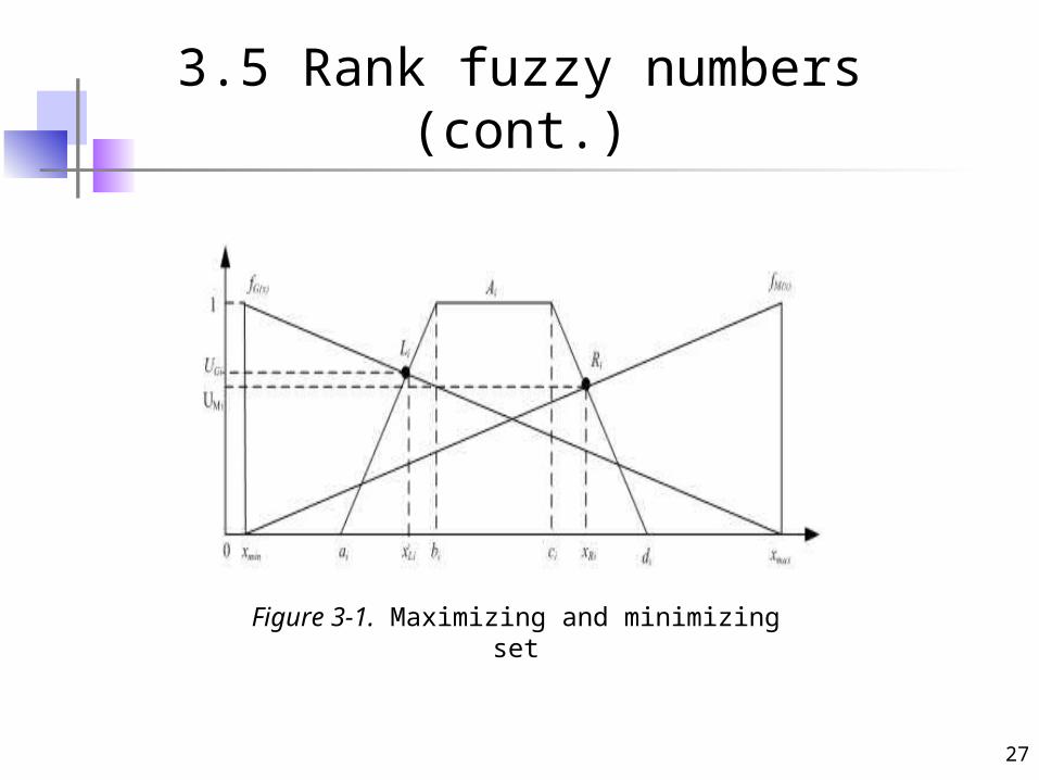
3.5 Rank fuzzy numbers (cont.)

Figure 3-1. Maximizing and minimizing set

28

3.5 Rank fuzzy numbers (cont.)

• Applying Eqs.(3.16)~ (3.22), the total utility of fuzzy number can be obtained as:

(3.23)

)(2

))]()((4)[()([

2

1

321

2

1

3213212

321321

iii

iiiRiiiiiiiii

ACC

OQQxACCBDDBDDI

. ])(2

))]()((4)[()(1

321

2

1

3213212

321321

iii

iiiLiiiiiiiii

CAA

QOOxCAADBBDBBi

, ~1, ))(1)((2

1)( niGUGUGU iNiMiT

iG

29

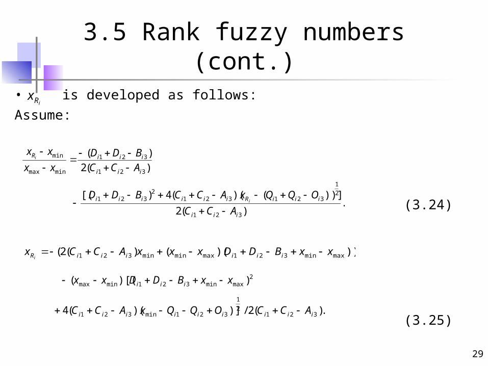
3.5 Rank fuzzy numbers (cont.)

• is developed as follows:

Assume:

(3.24)

(3.25)

iRx

)(2

)(

321

321

minmax

min

iii

iiiR

ACC

BDD

xx

xxi

.)(2

))]()((4)[(

321

2

1

3213212

321

iii

iiiRiiiiii

ACC

OQQxACCBDDi

)))(()(2( maxmin321maxminmin321 xxBDDxxxACCx iiiiiiRi

2maxmin321minmax ))[(( xxBDDxx iii

.)(2/)])((4 3212

1

321min321 iiiiiiiii ACCOQQxACC

30

3.5 Rank fuzzy numbers (cont.)

• is developed as follows:

Assume:

(3.26)

(3.27)

iLx

)(2

)(

321

321

maxmin

max

iii

iiiL

CAA

DBB

xx

xxi

.)(2

))]()((4)[(

321

2

1

3213212

321

iii

iiiLiiiiii

CAA

QOOxCAADBBi

)))(()(2( minmax321minmaxmax321 xxDBBxxxCAAx iiiiiiLi

2minmax321maxmin ))[(( xxDBBxx iii

. )(2/)])((4 3212

1

321max321 iiiiiiiii CAAQOOxCAA

31

NUMERICAL EXAMPLE

• 4.1 Ratings of alternatives versus qualitative

criteria

• 4.2 Normalization of quantitative criteria

• 4.3 Averaged weights of criteria

• 4.4 Development of membership function

• 4.5 Defuzzification

32

NUMERICAL EXAMPLE

• Assume that a logistics company is looking for a suitable city to set

up a new distribution center.

• Suppose three decision makers, D1, D2 and D3 of this company is

responsible for the evaluation of three distribution center

candidates, A1, A2 and A3.

33

Criteria

Qualitative criteria Quantitative criteria

Benefit Benefit Cost

Expansion possibility

Availability of acquirement

material

Closeness to demand market

Human resource

Square measure of area

Investment cost

Figure 4-1. Selected criteria

34

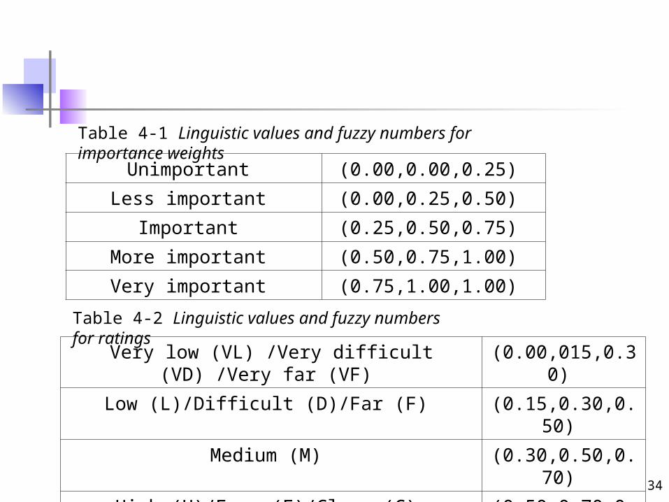
Unimportant (0.00,0.00,0.25)

Less important (0.00,0.25,0.50)

Important (0.25,0.50,0.75)

More important (0.50,0.75,1.00)

Very important (0.75,1.00,1.00)

Very low (VL) /Very difficult (VD) /Very far (VF) (0.00,015,0.30)

Low (L)/Difficult (D)/Far (F) (0.15,0.30,0.50)

Medium (M) (0.30,0.50,0.70)

High (H)/Easy (E)/Close (C) (0.50,0.70,0.85)

Very high (VH)/Very easy (VE)/Very close (VC) (0.70,0.85,1.00)

Table 4-1 Linguistic values and fuzzy numbers for importance weights

Table 4-2 Linguistic values and fuzzy numbers for ratings

35

4.1 Ratings of alternatives versus qualitative criteria

• Ratings of distribution center candidates versus qualitative criteria are given by decision makers as shown in Table 4-3. Through Eq. (3.1), averaged ratings of distribution center candidates versus qualitative criteria can be obtained as also displayed in Table 4-3.

Candidates Criteria D1 D2 D3Averaged

Ratings

A1

C1 VH H VH (0.63,0.80,0.95)C2 VE E M (0.50,0.68,0.85)C3 C VC VC (0.63,0.80,0.95)C4 M H H (0.43,0.63,0.80)

A2

C1 VH VH H (0.63,0.80,0.95)C2 M M E (0.37,0.57,0.75)

C3 C C VC (0.57,0.75,0.90)C4 VH VH VH (0.70,0.85,1.00)

A3

C1 L L H (0.27,0.43,0.62)C2 VE E VE (0.63,0.80,0.95)C3 M M C (0.37,0.57,0.75)C4 L M H (0.32,0.50,0.68)

36

4.2 Normalization of quantitative criteria

• Evaluation values under quantitative criteria are objective. Suppose values of distribution center candidates versus quantitative criteria are present as in Table 4-4.

Table 4-4 Values of distribution center candidates versus quantitative

criteria

CriteriaDistribution Center Candidates

Units

A1 A2 A3

C5 100 80 90 hectare

C6 2 5 10 million

37

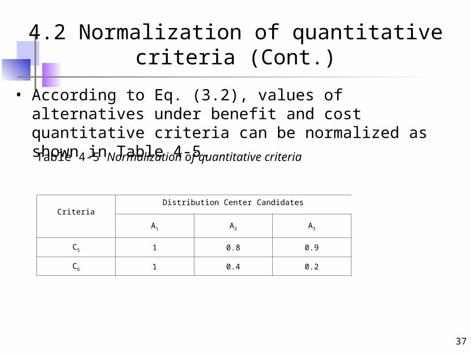
4.2 Normalization of quantitative criteria (Cont.)

• According to Eq. (3.2), values of alternatives under benefit and cost quantitative criteria can be normalized as shown in Table 4-5.

Table 4-5 Normalization of quantitative criteria

CriteriaDistribution Center Candidates

A1 A2 A3

C5 1 0.8 0.9

C6 1 0.4 0.2

38

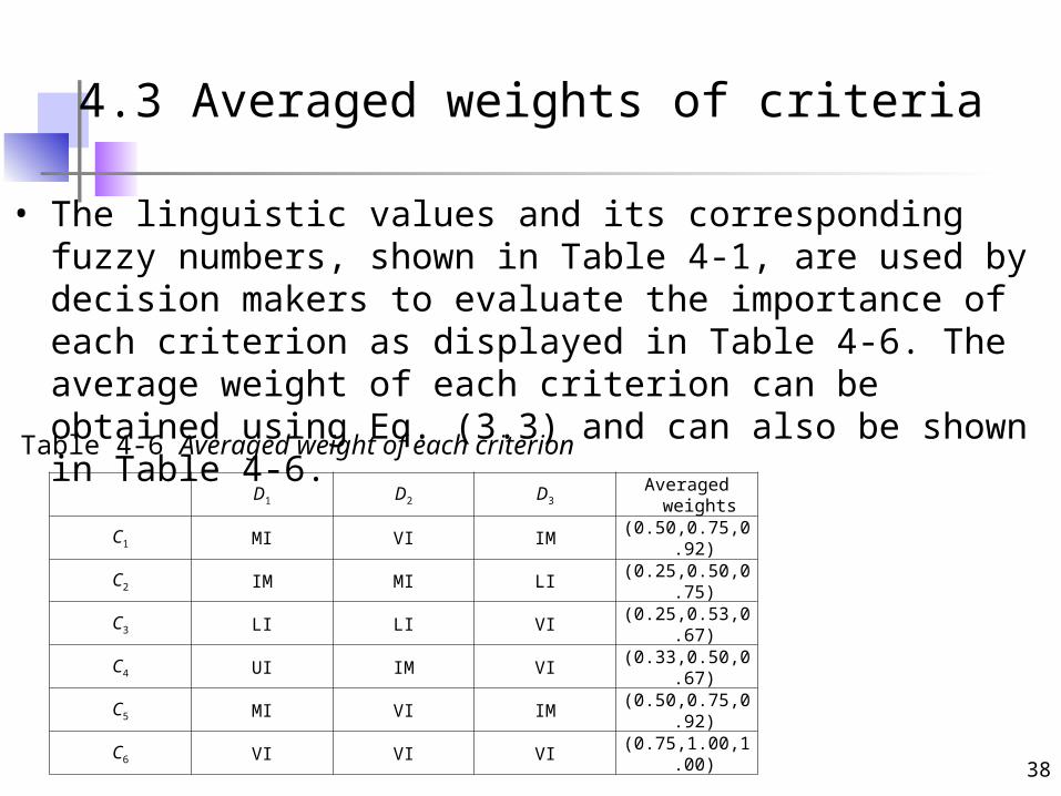
4.3 Averaged weights of criteria

• The linguistic values and its corresponding fuzzy numbers, shown in Table 4-1, are used by decision makers to evaluate the importance of each criterion as displayed in Table 4-6. The average weight of each criterion can be obtained using Eq. (3.3) and can also be shown in Table 4-6.

Table 4-6 Averaged weight of each criterion

D1 D2 D3 Averaged weights

C1 MI VI IM (0.50,0.75,0.92)

C2 IM MI LI (0.25,0.50,0.75)

C3 LI LI VI (0.25,0.53,0.67)

C4 UI IM VI (0.33,0.50,0.67)

C5 MI VI IM (0.50,0.75,0.92)

C6 VI VI VI (0.75,1.00,1.00)

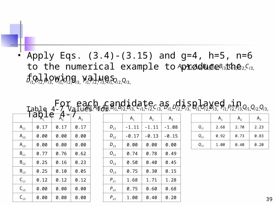
• Apply Eqs. (3.4)-(3.15) and g=4, h=5, n=6 to the numerical example to produce the following values

For each candidate as displayed in Table 4-7

39

1, 2, 3,i i iA A A 1, 2, 3,i i iB B B 1, 2, 3,i i iC C C

1, 2, 3,i i iD D D 1, 2, 3,i i iO O O 1, 2, 3,i i iP P P 1, 2, 3,i i iQ Q Q

Table 4-7 Values for 1, 2, 3,i i iA A A 1, 2, 3,i i iB B B 1, 2, 3,i i iC C C 1, 2, 3,i i iD D D 1, 2, 3,i i iO O O 1, 2, 3,i i iP P P 1, 2, 3,i i iQ Q Q

A1 A2 A3

Ai1 0.17 0.17 0.17

Ai2 0.00 0.00 0.00

Ai3 0.00 0.00 0.00

Bi1 0.77 0.76 0.62

Bi2 0.25 0.16 0.23

Bi3 0.25 0.10 0.05

Ci1 0.12 0.12 0.12

Ci2 0.00 0.00 0.00

Ci3 0.00 0.00 0.00

A1 A2 A3

Di1 -1.11 -1.11 -1.08

Di2 -0.17 -0.13 -0.15

Di3 0.00 0.00 0.00

Oi1 0.74 0.78 0.49

Oi2 0.50 0.40 0.45

Oi3 0.75 0.30 0.15

Pi1 1.68 1.71 1.28

Pi2 0.75 0.60 0.68

Pi3 1.00 0.40 0.20

A1 A2 A3

Qi1 2.68 2.70 2.23

Qi2 0.92 0.73 0.83

Qi3 1.00 0.40 0.20

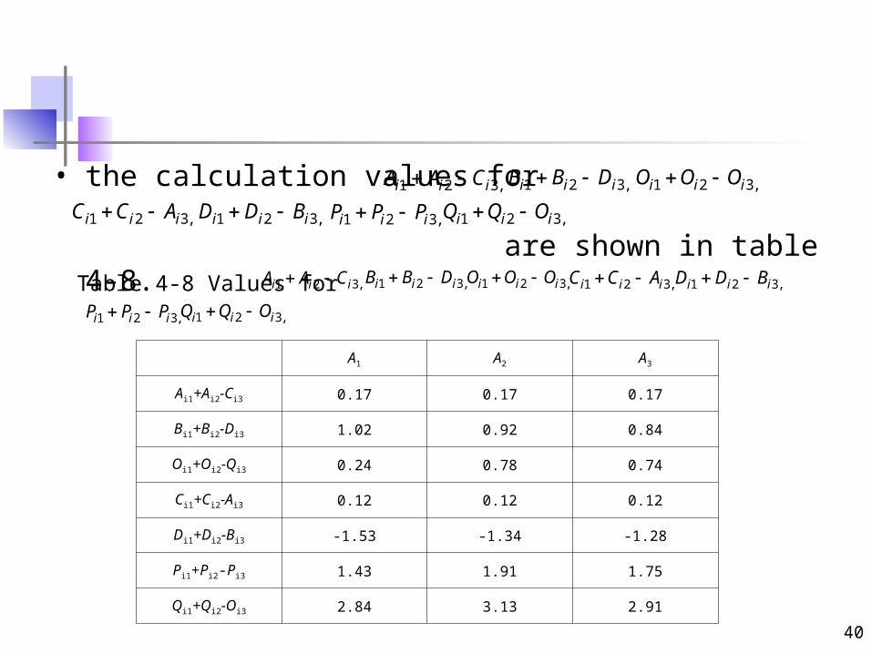
• the calculation values for are shown in table 4-8.

40

1 2 3,i i iA A C 1 2 3,i i iB B D 1 2 3,i i iO O O

1 2 3,i i iC C A 1 2 3,i i iD D B 1 2 3,i i iP P P 1 2 3,i i iQ Q O

Table 4-8 Values for 1 2 3,i i iA A C 1 2 3,i i iB B D 1 2 3,i i iO O O 1 2 3,i i iC C A 1 2 3,i i iD D B

1 2 3,i i iP P P 1 2 3,i i iQ Q O

A1 A2 A3

Ai1+Ai2-Ci3 0.17 0.17 0.17

Bi1+Bi2-Di3 1.02 0.92 0.84

Oi1+Oi2-Qi3 0.24 0.78 0.74

Ci1+Ci2-Ai3 0.12 0.12 0.12

Di1+Di2-Bi3 -1.53 -1.34 -1.28

Pi1+Pi2-Pi3 1.43 1.91 1.75

Qi1+Qi2-Oi3 2.84 3.13 2.91

41

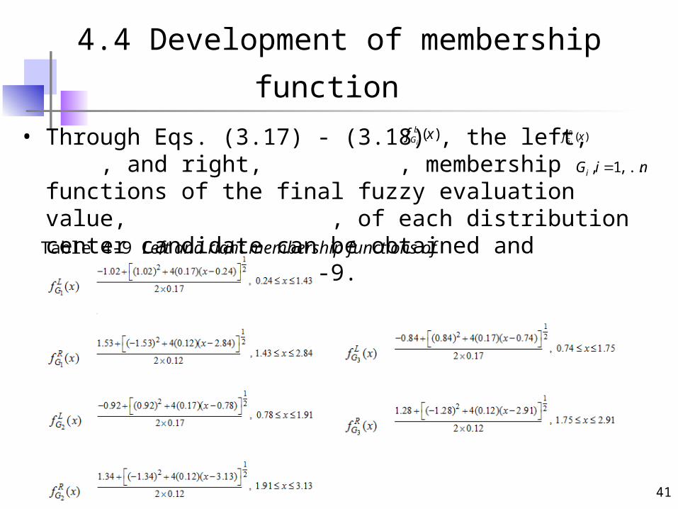
4.4 Development of membership function

• Through Eqs. (3.17) - (3.18) , the left, , and right, , membership functions of the final fuzzy evaluation value, , of each distribution center candidate can be obtained and displayed in Table 4-9.

)( xf LGi

)( xf RGi

niGi ,...,1,

Table 4-9 Left and right membership functions of Gi

42

4.5 Defuzzification

• By Eqs. (3.23)-(3.28) in Model development for defuzzification, the total utilities, and can be obtained and shown in Table 4-10.

Table 4-10 Total utilities and

Then according to values in Table 4-10, candidate A2 has the largest total utility, 0.551. Therefore becomes the most suitable distribution center candidate.

),( iT GU iRxiLx

),( iT GUiRx

iLx

2A

Alternatives T1 T2 T3

1.97 2.26 2.12

1.39 1.40 1.33

0.315 0.551 0.517

iRx

iLx

)( iT GU

43

CONCLUSIONS

• A fuzzy MCDM model is proposed for the evaluation and selection of the locations of distribution centers

• Chen’s maximizing set and minimizing set is applied to the model

in order to develop ranking formulae.

• Ranking formulae are clearly developed for better executing the decision making

• A numerical example is conducted to demonstrate the computational procedure and the feasibility of the proposed model.