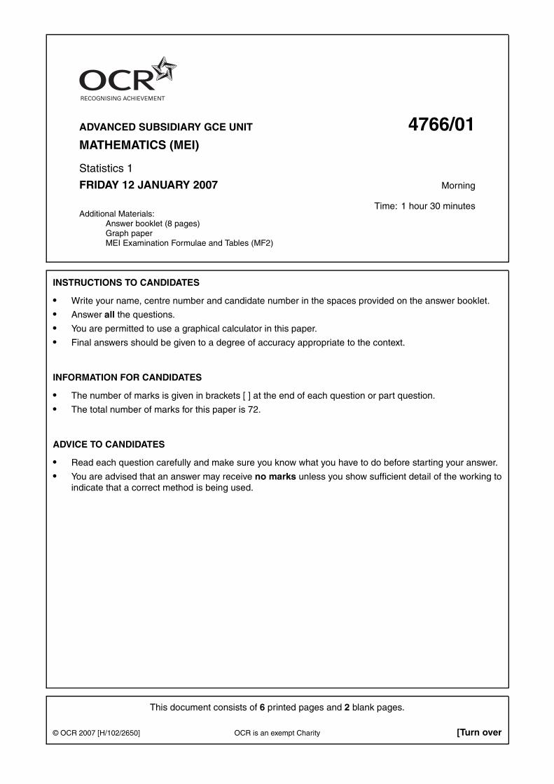
ADVANCED SUBSIDIARY GCE UNIT 4766/01MATHEMATICS (MEI)

Statistics 1

FRIDAY 12 JANUARY 2007 Morning

Time: 1 hour 30 minutesAdditional Materials:

Answer booklet (8 pages)Graph paperMEI Examination Formulae and Tables (MF2)

INSTRUCTIONS TO CANDIDATES

• Write your name, centre number and candidate number in the spaces provided on the answer booklet.

• Answer all the questions.

• You are permitted to use a graphical calculator in this paper.

• Final answers should be given to a degree of accuracy appropriate to the context.

INFORMATION FOR CANDIDATES

• The number of marks is given in brackets [ ] at the end of each question or part question.

• The total number of marks for this paper is 72.

ADVICE TO CANDIDATES

• Read each question carefully and make sure you know what you have to do before starting your answer.

• You are advised that an answer may receive no marks unless you show sufficient detail of the working toindicate that a correct method is being used.

This document consists of 6 printed pages and 2 blank pages.

© OCR 2007 [H/102/2650] OCR is an exempt Charity [Turn over

2

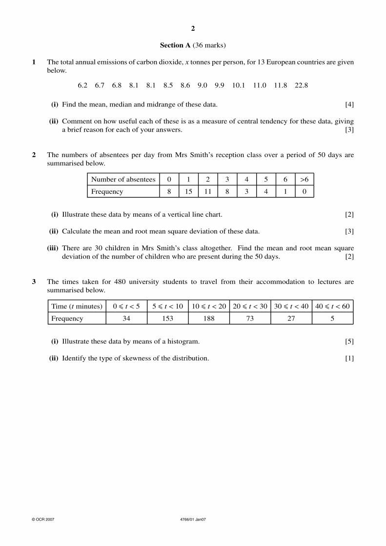
Section A (36 marks)

1 The total annual emissions of carbon dioxide, x tonnes per person, for 13 European countries are givenbelow.

6.2 6.7 6.8 8.1 8.1 8.5 8.6 9.0 9.9 10.1 11.0 11.8 22.8

(i) Find the mean, median and midrange of these data. [4]

(ii) Comment on how useful each of these is as a measure of central tendency for these data, givinga brief reason for each of your answers. [3]

2 The numbers of absentees per day from Mrs Smith’s reception class over a period of 50 days aresummarised below.

Number of absentees 0 1 2 3 4 5 6 >6

Frequency 8 15 11 8 3 4 1 0

(i) Illustrate these data by means of a vertical line chart. [2]

(ii) Calculate the mean and root mean square deviation of these data. [3]

(iii) There are 30 children in Mrs Smith’s class altogether. Find the mean and root mean squaredeviation of the number of children who are present during the 50 days. [2]

3 The times taken for 480 university students to travel from their accommodation to lectures aresummarised below.

Time (t minutes) 0 ≤ t < 5 5 ≤ t < 10 10 ≤ t < 20 20 ≤ t < 30 30 ≤ t < 40 40 ≤ t < 60

Frequency 34 153 188 73 27 5

(i) Illustrate these data by means of a histogram. [5]

(ii) Identify the type of skewness of the distribution. [1]

© OCR 2007 4766/01 Jan07

3

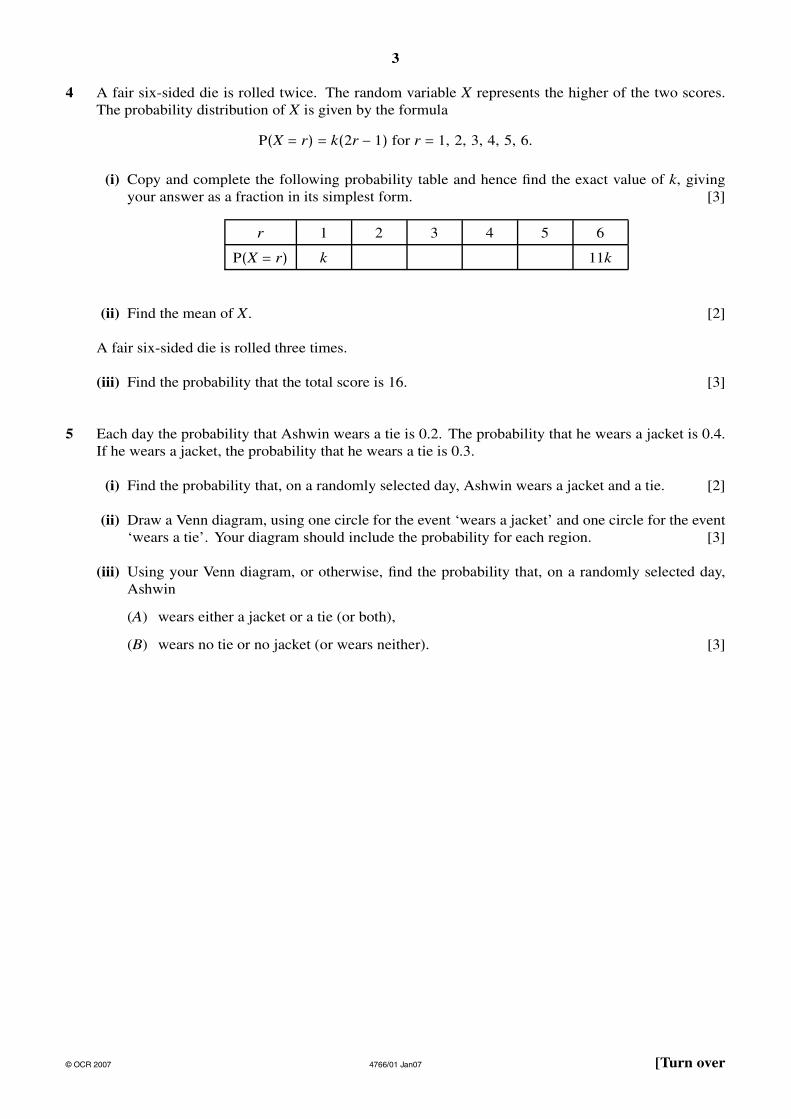
4 A fair six-sided die is rolled twice. The random variable X represents the higher of the two scores.The probability distribution of X is given by the formula

P(X = r) = k(2r − 1) for r = 1, 2, 3, 4, 5, 6.

(i) Copy and complete the following probability table and hence find the exact value of k, givingyour answer as a fraction in its simplest form. [3]

r 1 2 3 4 5 6

P(X = r) k 11k

(ii) Find the mean of X. [2]

A fair six-sided die is rolled three times.

(iii) Find the probability that the total score is 16. [3]

5 Each day the probability that Ashwin wears a tie is 0.2. The probability that he wears a jacket is 0.4.If he wears a jacket, the probability that he wears a tie is 0.3.

(i) Find the probability that, on a randomly selected day, Ashwin wears a jacket and a tie. [2]

(ii) Draw a Venn diagram, using one circle for the event ‘wears a jacket’ and one circle for the event‘wears a tie’. Your diagram should include the probability for each region. [3]

(iii) Using your Venn diagram, or otherwise, find the probability that, on a randomly selected day,Ashwin

(A) wears either a jacket or a tie (or both),

(B) wears no tie or no jacket (or wears neither). [3]

© OCR 2007 4766/01 Jan07 [Turn over

4

Section B (36 marks)

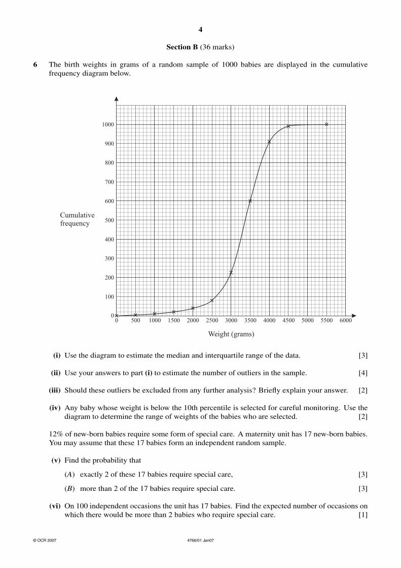
6 The birth weights in grams of a random sample of 1000 babies are displayed in the cumulativefrequency diagram below.

(i) Use the diagram to estimate the median and interquartile range of the data. [3]

(ii) Use your answers to part (i) to estimate the number of outliers in the sample. [4]

(iii) Should these outliers be excluded from any further analysis? Briefly explain your answer. [2]

(iv) Any baby whose weight is below the 10th percentile is selected for careful monitoring. Use thediagram to determine the range of weights of the babies who are selected. [2]

12% of new-born babies require some form of special care. A maternity unit has 17 new-born babies.You may assume that these 17 babies form an independent random sample.

(v) Find the probability that

(A) exactly 2 of these 17 babies require special care, [3]

(B) more than 2 of the 17 babies require special care. [3]

(vi) On 100 independent occasions the unit has 17 babies. Find the expected number of occasions onwhich there would be more than 2 babies who require special care. [1]

© OCR 2007 4766/01 Jan07

5

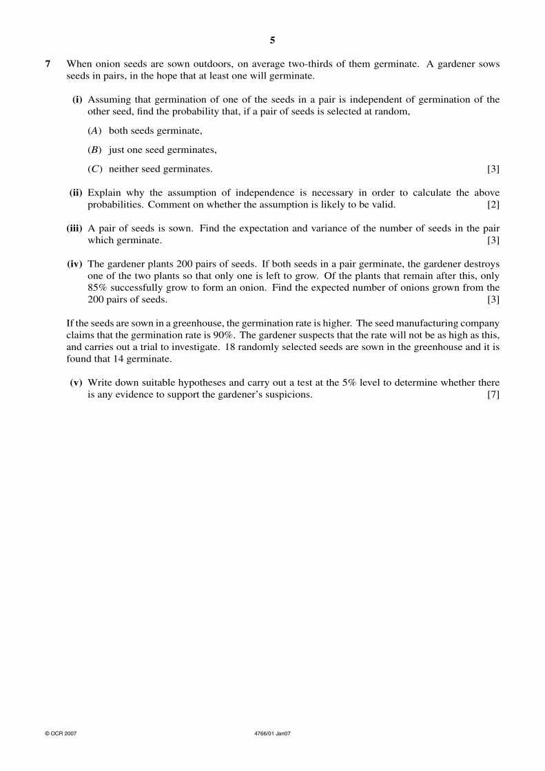
7 When onion seeds are sown outdoors, on average two-thirds of them germinate. A gardener sowsseeds in pairs, in the hope that at least one will germinate.

(i) Assuming that germination of one of the seeds in a pair is independent of germination of theother seed, find the probability that, if a pair of seeds is selected at random,

(A) both seeds germinate,

(B) just one seed germinates,

(C) neither seed germinates. [3]

(ii) Explain why the assumption of independence is necessary in order to calculate the aboveprobabilities. Comment on whether the assumption is likely to be valid. [2]

(iii) A pair of seeds is sown. Find the expectation and variance of the number of seeds in the pairwhich germinate. [3]

(iv) The gardener plants 200 pairs of seeds. If both seeds in a pair germinate, the gardener destroysone of the two plants so that only one is left to grow. Of the plants that remain after this, only85% successfully grow to form an onion. Find the expected number of onions grown from the200 pairs of seeds. [3]

If the seeds are sown in a greenhouse, the germination rate is higher. The seed manufacturing companyclaims that the germination rate is 90%. The gardener suspects that the rate will not be as high as this,and carries out a trial to investigate. 18 randomly selected seeds are sown in the greenhouse and it isfound that 14 germinate.

(v) Write down suitable hypotheses and carry out a test at the 5% level to determine whether thereis any evidence to support the gardener’s suspicions. [7]

© OCR 2007 4766/01 Jan07

6

BLANK PAGE

4766/01 Jan07

7

BLANK PAGE

4766/01 Jan07

8

Permission to reproduce items where third-party owned material protected by copyright is included has been sought and cleared where possible. Every reasonableeffort has been made by the publisher (UCLES) to trace copyright holders, but if any items requiring clearance have unwittingly been included, the publisher willbe pleased to make amends at the earliest possible opportunity.

OCR is part of the Cambridge Assessment Group. Cambridge Assessment is the brand name of University of Cambridge Local Examinations Syndicate (UCLES),which is itself a department of the University of Cambridge.

© OCR 2007 4766/01 Jan07

63

Mark Scheme 4766January 2007

4766 Mark Scheme January 2007

64

GENERAL INSTRUCTIONS Marks in the mark scheme are explicitly designated as M, A, B, E or G. M marks ("method") are for an attempt to use a correct method (not merely for stating the method). A marks ("accuracy") are for accurate answers and can only be earned if corresponding M mark(s) have been earned. Candidates are expected to give answers to a sensible level of accuracy in the context of the problem in hand. The level of accuracy quoted in the mark scheme will sometimes deliberately be greater than is required, when this facilitates marking. B marks are independent of all others. They are usually awarded for a single correct answer. E marks ("explanation") are for explanation and/or interpretation. These will frequently be sub divisible depending on the thoroughness of the candidate's answer. G marks ("graph") are for completing a graph or diagram correctly.

• Insert part marks in right-hand margin in line with the mark scheme. For fully correct parts tick the answer. For partially complete parts indicate clearly in the body of the script where the marks have been gained or lost, in line with the mark scheme.

• Please indicate incorrect working by ringing or underlining as appropriate.

• Insert total in right-hand margin, ringed, at end of question, in line with the mark scheme.

• Numerical answers which are not exact should be given to at least the accuracy shown.

Approximate answers to a greater accuracy may be condoned.

• Probabilities should be given as fractions, decimals or percentages.

• FOLLOW-THROUGH MARKING SHOULD NORMALLY BE USED WHEREVER POSSIBLE. There will, however, be an occasional designation of 'c.a.o.' for "correct answer only".

• Full credit MUST be given when correct alternative methods of solution are used. If errors

occur in such methods, the marks awarded should correspond as nearly as possible to equivalent work using the method in the mark scheme.

• The following notation should be used where applicable:

FT Follow-through marking

BOD Benefit of doubt

ISW Ignore subsequent working

4766 Mark Scheme January 2007

65

Q1 (i)

Mean = 127.6/13 = 9.8 Median = 8.6 Midrange = 14.5

M1 for 127.6/13 soi A1 CAO B1 CAO B1 CAO

4 (ii)

Mean slightly inflated due to the outlier Median good since it is not affected by the outlier Midrange poor as it is highly inflated due to the outlier

B1 B1 B1

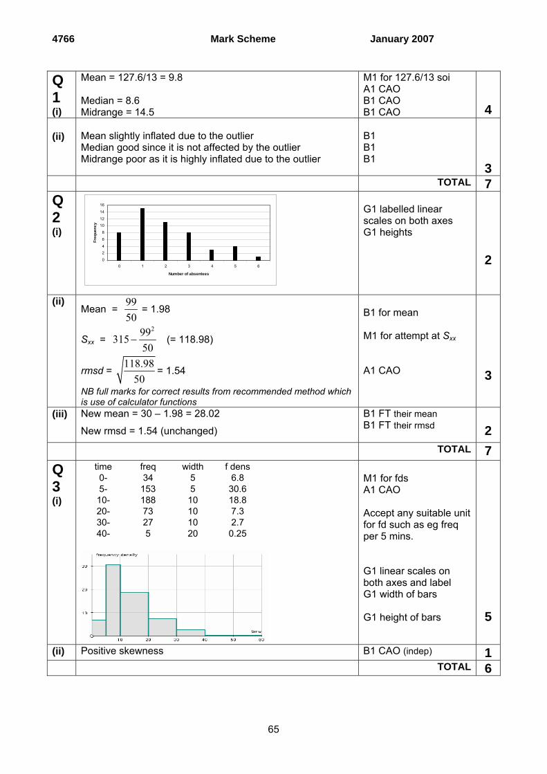
3 TOTAL 7 Q2 (i)

0

24

6

8

10

12

14

16

0 1 2 3 4 5 6

Number of absentees

Freq

uenc

y

G1 labelled linear scales on both axes G1 heights

2

(ii) Mean =

9950

= 1.98

Sxx = 299315

50− (= 118.98)

rmsd = 118.98

50= 1.54

NB full marks for correct results from recommended method which is use of calculator functions

B1 for mean M1 for attempt at Sxx

A1 CAO

3

(iii) New mean = 30 – 1.98 = 28.02

New rmsd = 1.54 (unchanged)

B1 FT their mean B1 FT their rmsd

2

TOTAL 7

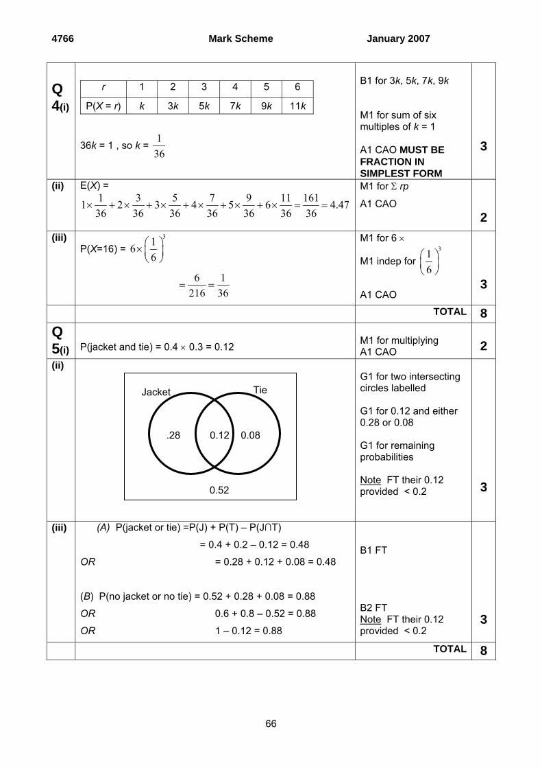
Q3 (i)

time freq width f dens 0- 34 5 6.8 5- 153 5 30.6 10- 188 10 18.8 20- 73 10 7.3 30- 27 10 2.7 40- 5 20 0.25

M1 for fds A1 CAO Accept any suitable unit for fd such as eg freq per 5 mins. G1 linear scales on both axes and label G1 width of bars G1 height of bars

5

(ii) Positive skewness B1 CAO (indep) 1 TOTAL 6

4766 Mark Scheme January 2007

66

Q4(i)

r 1 2 3 4 5 6

P(X = r) k 3k 5k 7k 9k 11k

36k = 1 , so k = 136

B1 for 3k, 5k, 7k, 9k M1 for sum of six multiples of k = 1 A1 CAO MUST BE FRACTION IN SIMPLEST FORM

3

(ii) E(X) = 1 3 5 7 9 11 1611 2 3 4 5 6 4.4736 36 36 36 36 36 36

× + × + × + × + × + × = =

M1 for Σ rp

A1 CAO

2

(iii) P(X=16) =

3166

⎛ ⎞× ⎜ ⎟⎝ ⎠

6 1

216 36= =

M1 for 6 ×

M1 indep for 31

6⎛ ⎞⎜ ⎟⎝ ⎠

A1 CAO

3

TOTAL 8

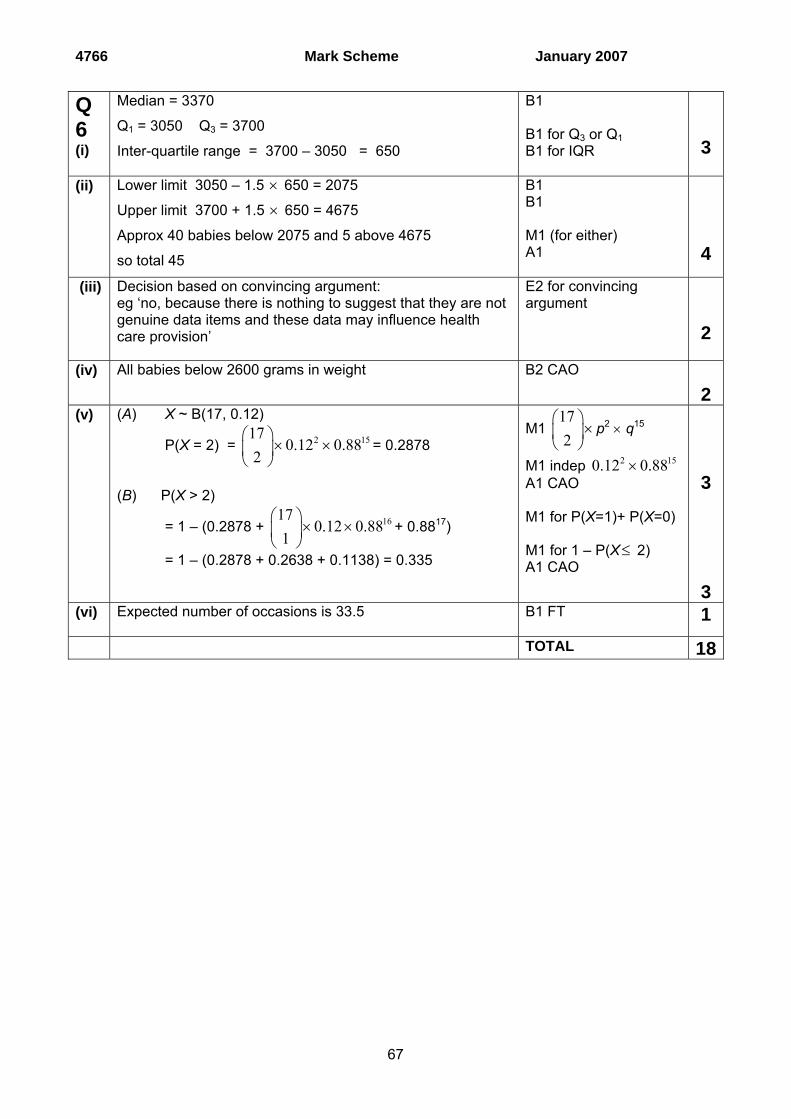
Q5(i)

P(jacket and tie) = 0.4 × 0.3 = 0.12

M1 for multiplying A1 CAO

2

(ii)

G1 for two intersecting circles labelled G1 for 0.12 and either 0.28 or 0.08 G1 for remaining probabilities Note FT their 0.12 provided < 0.2

3

(iii) (A) P(jacket or tie) =P(J) + P(T) – P(J∩T)

= 0.4 + 0.2 – 0.12 = 0.48

OR = 0.28 + 0.12 + 0.08 = 0.48

(B) P(no jacket or no tie) = 0.52 + 0.28 + 0.08 = 0.88

OR 0.6 + 0.8 – 0.52 = 0.88

OR 1 – 0.12 = 0.88

B1 FT B2 FT Note FT their 0.12 provided < 0.2

3

TOTAL 8

.28 0.12

0.52

Jacket Tie

0.08

4766 Mark Scheme January 2007

67

Q6 (i)

Median = 3370

Q1 = 3050 Q3 = 3700

Inter-quartile range = 3700 – 3050 = 650

B1 B1 for Q3 or Q1 B1 for IQR

3

(ii) Lower limit 3050 – 1.5 × 650 = 2075

Upper limit 3700 + 1.5 × 650 = 4675

Approx 40 babies below 2075 and 5 above 4675

so total 45

B1 B1 M1 (for either) A1

4 (iii) Decision based on convincing argument:

eg ‘no, because there is nothing to suggest that they are not genuine data items and these data may influence health care provision’

E2 for convincing argument

2

(iv) All babies below 2600 grams in weight B2 CAO 2

(v) (A) X ~ B(17, 0.12)

P(X = 2) = 2 15170.12 0.88

2⎛ ⎞

× ×⎜ ⎟⎝ ⎠

= 0.2878

(B) P(X > 2)

= 1 – (0.2878 + 16170.12 0.88

1⎛ ⎞

× ×⎜ ⎟⎝ ⎠

+ 0.8817)

= 1 – (0.2878 + 0.2638 + 0.1138) = 0.335

M1 172

⎛ ⎞×⎜ ⎟

⎝ ⎠p2 × q15

M1 indep 2 150.12 0.88× A1 CAO M1 for P(X=1)+ P(X=0) M1 for 1 – P(X ≤ 2) A1 CAO

3

3

(vi) Expected number of occasions is 33.5

B1 FT 1 TOTAL 18

4766 Mark Scheme January 2007

68

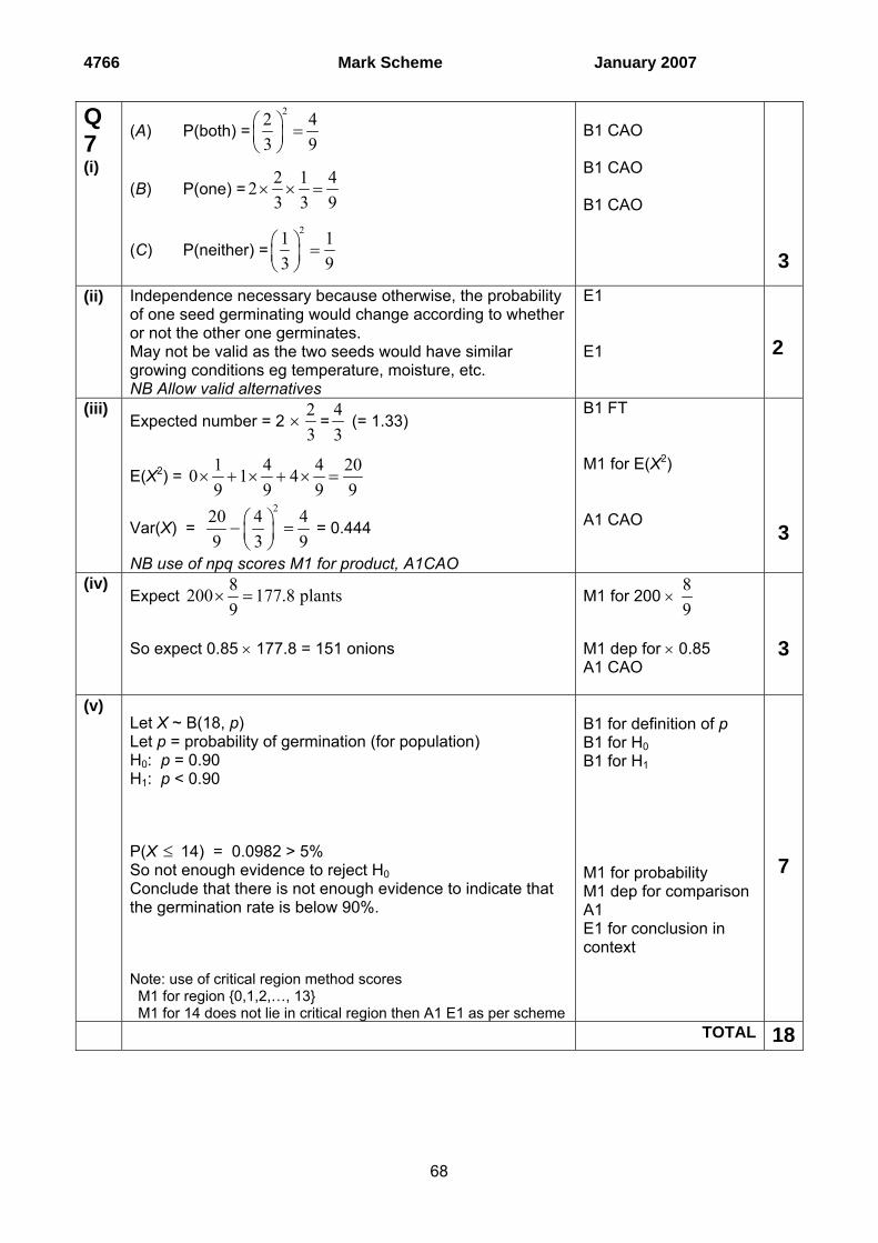
Q7 (i)

(A) P(both) =22 4

3 9⎛ ⎞ =⎜ ⎟⎝ ⎠

(B) P(one) =2 1 423 3 9

× × =

(C) P(neither) =21 1

3 9⎛ ⎞ =⎜ ⎟⎝ ⎠

B1 CAO B1 CAO B1 CAO

3 (ii) Independence necessary because otherwise, the probability

of one seed germinating would change according to whether or not the other one germinates. May not be valid as the two seeds would have similar growing conditions eg temperature, moisture, etc. NB Allow valid alternatives

E1 E1

2

(iii) Expected number = 2 ×

23

=43

(= 1.33)

E(X2) = 1 4 4 200 1 49 9 9 9

× + × + × =

Var(X) = 220 4 4

9 3 9⎛ ⎞− =⎜ ⎟⎝ ⎠

= 0.444

NB use of npq scores M1 for product, A1CAO

B1 FT M1 for E(X2) A1 CAO

3

(iv) Expect

8200 177.8 plants9

× =

So expect 0.85 × 177.8 = 151 onions

M1 for 200 × 89

M1 dep for × 0.85 A1 CAO

3

(v) Let X ~ B(18, p) Let p = probability of germination (for population) H0: p = 0.90 H1: p < 0.90

P(X ≤ 14) = 0.0982 > 5% So not enough evidence to reject H0 Conclude that there is not enough evidence to indicate that the germination rate is below 90%.

Note: use of critical region method scores M1 for region {0,1,2,…, 13} M1 for 14 does not lie in critical region then A1 E1 as per scheme

B1 for definition of p B1 for H0 B1 for H1 M1 for probability M1 dep for comparison A1 E1 for conclusion in context

7

TOTAL 18

Report on the units taken in January 2007

4766 - Statistics 1 General Comments

The paper attracted a fairly wide range of responses, although there were relatively few scripts with either exceptionally high or exceptionally low scores. However candidates did seem to perform at a somewhat lower level than in recent sessions. There was no evidence to suggest that candidates had insufficient time to attempt all questions, apart from those who chose very long winded methods in more than one question. Answers were often well presented but a good number of candidates do not appreciate the implications of using rounded answers in subsequent calculations. Most candidates gave good answers to and were able to earn substantial marks from Questions 1i, 2, 3, 4, and parts of 6 and 7. Question 5 was not well answered; as was reported last summer, candidates were again evidently unclear about how to manipulate probabilities in a Venn diagram and many scored at best 3 out of 8 marks. The performance on question 6 (i) – (iii) was also variable, with many candidates making errors in accurately reading the graph scales and in calculating outliers. Several parts of Question 7 were not well answered. Many candidates are still not meeting the requirement to define p in words in the context of questions on hypothesis testing and many candidates are also using point probabilities rather than tail probabilities. Comments on Individual Questions Section A 1 Carbon dioxide emissions; mean, median, midrange and comments.

(i) The mean and median were almost always correct but the midrange was

confused with the range or IQR. Many candidates calculated (max-min)/2 = 8.3 instead of (max + min)/2 = 14.5.

(ii) Despite the question saying ‘for these data’, most comments did not relate specifically to the data, but were general in nature. Examiners were looking for two aspects here: the suitability of each measure of central tendency (i.e. good, poor, useful, etc) and how each measure was or was not influenced by the outlier of 22.8. Many candidates thought that the midrange was a measure of spread in the data. Others felt that the mean and/or midrange were good measures ‘because they detected outliers’. Relatively few convincing responses were seen.

2 Absentees; vertical line chart, mean and root mean squared deviation, calculation of new mean and rmsd.

(i) The vertical line chart was almost without exception correctly drawn, with only a tiny minority failing to label the axes.

(ii) The mean and rmsd were generally tackled well; the main errors seen were failure to take the square root: using an (n – 1) divisor in the rmsd instead of n, dividing by 30 (the number of pupils in the class) or dividing by 21 (from 0+1+2+3+4+5+6) instead of dividing by 50 (the number of days the data were collected over).

29

Report on the units taken in January 2007 (iii) All that was required here was to be aware that ‘new mean = 30 – original mean’

and ‘new rmsd = original rmsd’. Unfortunately very few candidates recognised the transformation x → 30 – x , and instead most produced inordinately long solutions by re-calculating, often going wrong in the process. The fact that only 2 marks were available should have alerted candidates that this did not warrant a further 2 pages of calculations.

3 Travel times; histogram and skewness.

(i) There were many very good responses to this question with full marks often achieved for the whole question. Some candidates who favoured the frequency per 5 minutes or frequency per 10 minutes approach failed to label the vertical axis of the histogram as such but instead simply used a label of ‘frequency density’, thus losing a mark. This label only gains credit when the candidate is using frequency per unit x value. Some of the weaker candidates used non-linear scales on the horizontal axis or labelled the axis with a series of inequalities ( 0 ≤ t <5, 5 ≤ t < 10, etc) rather than the correct linear scale. Only a small minority drew a frequency diagram.

(ii) Almost all candidates recognised the positive skewness for the shape of the distribution.

4 Dice; evaluating k; calculation of E(X), probability.

(i) Most candidates correctly found k = 1/36 although there were a few sightings of 1/35 or 1/37.

(ii) The expectation E(X) was almost always found correctly but there were many candidates who then went on to calculate E(X) / n, for some value of n, usually with n = 6 or n = 21.

(iii) Many candidates used the previous probabilities instead of 1/6, 1/6, 1/6. A significant minority could not identify the 6 ways of getting a total of 16, often only coming up with 2 ways or even 12 ways. Numbers that did not add up to 16 were sometimes seen, especially (4, 4, 4).

5 Wearing a tie or jacket, conditional probability, Venn diagram, probability calculations.

(i) Many candidates were unable to correctly deal with the conditional probability aspect of this question and instead of the required 0.4 × 0.3 = 0.12 in part (i), answers of 0.08 or 0.06 from 0.4 × 0.2 or 0.3 × 0.2 respectively were often seen.

(ii) Disappointingly, the vast majority of candidates produced an incorrect Venn diagram with the 0.4 placed inside the ‘jacket circle’ and the 0.2 placed inside the ‘tie circle’ instead of 0.28 and 0.08 respectively. In many cases the sum of the probabilities in the diagram was not one and probabilities were sometimes omitted. This is a relatively straightforward concept, but centres would be advised to deal very carefully with it when preparing candidates as they seem to have a great deal of difficulty with it. Such errors in the Venn diagram usually make it impossible to allow follow through marks in the next part of the question and so candidates lose a significant number of marks. There have now been 3 questions on Venn diagrams and probability in recent examinations but this remains an area where centres need to improve candidates’ understanding of the concepts and their labelling of diagrams.

30

Report on the units taken in January 2007 (iii) All sorts of errors were seen in here, but in (B) a common misconception was 1 –

answer (A). Section B 6) Birth weights; Cumulative frequency, median, IQR, outliers, percentiles,

binomial distribution, expected value.

(i) Many correct answers were seen although a substantial number of candidates were unable to read the scales accurately in order to find the median or quartiles. The most common error was the belief that 1 small square on the vertical scale was 10 instead of 20, thus leading to half the correct number of outliers in (ii). In view of the fact that these topics are examined at Intermediate Tier GCSE, significant penalties were imposed on candidates who did not read the scales correctly.

(ii) The definition of an outlier still remains unclear for a large number of candidates, with many thinking it is defined as median ± 1.5 IQR, or UQ + 2IQR, LQ - 2IQR or UQ + IQR, LQ – IQR or median ± 2 IQR instead of the correct LQ -1.5 IQR, UQ + 1.5 IQR.

(iii) The comments about outliers were often vague. The fact that in such a large data set a considerable number of genuine data values were likely to lie outside the limits was rarely mentioned. Equally only a few candidates made a reference to either premature or overweight babies or mentioned the relevance of the purpose for which the data was being used (eg health care provision).

(iv) The 10th percentile was very often correct although occasionally 2,500 or 550 were seen instead of 2600.

(v) This was usually very well answered with only a few candidates attempting incorrectly to use binomial tables by approximating 0.12 as 0.1. In fact most candidates seemed happier with this AS work than with the GCSE work earlier in the question. In part (B) the most common errors were 1 – [ P(0) + P(1) ] or 1 – [ P(1) + P(2)] instead of the correct 1 – [ P(0) + P(1) + P(2)].

(vi) Nearly all candidates found 100 × answer (v) (B) but occasionally the 100 was replaced by 17.

7) Germination and growth of onion seeds; binomial distribution, independence, calculation of E(X) and Var(X), expected frequency, hypothesis test on the binomial distribution.

(i) This was often correct but failure to multiply by 2 in (B) sometimes resulted in an answer of 2/9.

(ii) Many candidates gave good explanations here, although some failed to mention that lack of independence would mean that the probability of one event would be altered by the occurrence of the other event. It was very pleasing to see some candidates state that independence is a required condition for the use of the binomial distribution.

(iii) Most candidates calculated both expectation and variance correctly, although some inaccuracy was seen when candidates used decimal probabilities.

(iv) There was a great deal of confusion between ‘the number of seeds’ and ‘the

number of pairs of seeds’ with many halving when they should not have. Some 31

Report on the units taken in January 2007

only considered the pairs where both germinate, with 113.33 being a common wrong answer, for which some credit was awarded.

(v) It is pleasing to note that many candidates stated their hypotheses in symbolic form. However, as in previous papers, very few candidates defined the parameter ‘p’. Previous reports have referred to the importance of this matter. There are three marks available for the correct statement of hypotheses, including the definition of the p. Many candidates correctly evaluated P(X ≤ 14) = 0.0982 as the tail probability but some then made an erroneous statement along the lines of ‘0.0982 is not in the critical region at the 5% significance level’. It is important for centres to stress to candidates that the critical region contains only x-values and NOT p –values. However a pleasing number of candidates did explicitly show a correct comparison of 0.0982 with 0.05. Overall the work on hypothesis testing is slowly improving year by year but there are still too many candidates who base their arguments on point probabilities instead of tail probabilities.

32