adfa, p. 1, 2015.

© Springer-Verlag Berlin Heidelberg 2015

Adaptive UKF-SLAM based on Magnetic Gradient In-

version Method for Underwater Navigation

Meng Wu1*

, Jian Yao1

1School of Remote Sensing and Information Engineering, Wuhan University, Wuhan

430079, P.R. China

*E-mail: wumenghust911@gmail.com

ABSTRACT. Consider the two characteristics: (1) Simultaneous loca-

lization and mapping (SLAM) is a popular algorithm for autonom-

ous underwater vehicle, but visual SLAM is significantly influenced

by weak illumination. (2)Geomagnetism-aided navigation and gravi-

ty-aided navigation are equally important methods in the field of

vehicle navigation, but both are affected heavily by time-varying

noises and terrain fluctuations. However, magnetic gradient vector

can avoid the influence of time-varying noises, and is less affected

by terrain fluctuations. To this end, we propose an adaptive SLAM-

based magnetic gradient aided navigation with the following advan-

tages: (1) Adaptive SLAM is an efficient way to deal with uncertain-

ty of the measurement model. (2) Magnetic gradient inversion equa-

tion is a good alternative to be used as measurement equation in vis-

ual SLAM-denied environment. Experimental results show that our

proposed method is an effective solution, combining magnetic gra-

dient information with SLAM.

Keywords: Adaptive SLAM; Magnetic gradient vector; Magnetic gra-dient inversion equation.

Introduction

The simultaneous localization and mapping (SLAM) algorithm was first proposed

by Smith and Cheeseman in 1988 to provide localization and map building for

mobile vehicles, and first used for an unmanned underwater vehicle (UUV) navi-

gation in September 1997 in a collaborative project between the Naval Undersea

Warfare Center (NUWC) and Groupe d’Etudes Sous-Marines de l’Atlantique

(GESMA). The objective of using SLAM was to get a UUV starting in an un-

known location and without previous knowledge of the environment, to build a

map via its onboard sensors and then use the same map to compute the vehicle’s

location. In general, SLAM is widely used in visual navigation because vision is

the richest source of information from our environment [1][3]. The visual SLAM

techniques can be classified into using stereo camera [4][5] and monocular cam-

era [6-9].

From [2], it is clear that visual SLAM has its disadvantages in mobile vehicle,

which is affected greatly by illumination and camera pose. If a camera is in an

environment with poor illumination, visual signals cannot be obtained exactly to

be used as landmarks in visual SLAM, and a large measurement bias from a cam-

era cannot guarantee that the unscented Kalman filter (UKF)-SLAM has a good

convergence [16]. Finally, the estimated location cannot be accurate enough. In

particular, in the underwater environment, visual signals from stereo cameras are

easily distracted by weak illumination, which brings large measurement errors

into UKF-SLAM. Compared with the visual SLAM method, geophysical naviga-

tion approach is less affected by weak illumination, and is more suitable for the

autonomous underwater vehicle to acquire navigation updates by surfacing or

nearly surfacing [10][11]. Therefore, SLAM based on geophysical information is

an alternative in cases of visual signal drop-off. Liu et al. introduced a kind of

SLAM-based geomagnetic aided inertial navigation method to improve the accu-

racy of navigation and localization system [12]. Wang et al. combine geomagnetic

navigation algorithm together with SLAM to realize an autonomous navigation

system [13].

In the field of underwater object detection based on magnetic gradient tensor, Yu

Huang et al. proposed a localization method combined with magnetic gradient

tensor and draft depth [17]. Hao yan-ling et al. put forward an existing solution,

where the geomagnetic anomaly is inversed a magnetic dipole target and the rela-

tive position of the vehicle is determined by magnetic magnitude and gradients of

targets [18].

Considering various kinds of time-varying noises and terrain fluctuations, and

especially given that the variations in gravity or geomagnetism are insufficient in

some areas, we add magnetic gradient information into SLAM to improve the

accuracy of UKF-SLAM. In our method, the magnetic gradient values of land-

marks are measured by seven magnetometers which are installed on an underwa-

ter vehicle. According to magnetic gradient values, and combining a method from

[18][19], it is easy to obtain a relative position between a landmark and underwa-

ter vehicle. Then, an adaptive UKF is combined with SLAM to find a series of

optimal estimations for the underwater vehicle in different discrete times. Accord-

ing to such estimations, the vehicle can navigate itself without any reference maps.

This paper is organized as follows. In Section 2, the state and measurement mod-

els of a navigation system are introduced and analyzed. In section 3, the adaptive

UKF-SLAM algorithm is presented. In Section 4, experiment and stimulation

results are discussed. Conclusions and future work are summarized in Section 5.

1 Introduction of State and Measurement Equations

1.1 Introduction of State Equation

System state equation can be described in a kind of vehicle kinematics which is

given in the below form:

1

1

1

1

1 1

1

1

1

( 1) ( )

cos sin

sin cos

,

t t t t tt

t t t t tt

t t t

t t

t t t t t t

t t

t t

t t

i t i t

t

x u T v Tx

y u T v Ty

z z T

rT

X u X u n u n

v v

r r

P P

X

it[ , , , ], , , , ,

T

t t t t t t t tx y z u v r P

(1)

Whereit

[ , , , ], , , , ,T

t t t t t t t t tPX x y z u v r includes the position and heading of

underwater vehicle and the coordinates of a landmark ( itp ). , , ,t t t t

u v r are the

line velocity and angle velocity of the underwater vehicle and T is the sample

time. tn is system noise with covariance matrix given by R.

T

ttjjt jt

t t

E R

E

qq nn

qn

(2)

In the underwater environment, the method in [14] is a good solution to calculate

relative distance and orientation between a landmark and underwater vehicle.

The coordinates of a landmark is as follows:

itit

ityp x

(3)

Where itx and ity stand for the ith

landmark’s position information at the time t

in the direction of x and y, respectively. In general, the position of a static land-

mark varies minimally in the different time t

,( )1 1, 2, ,i t it ip p p i N (4)

1.2 Introduction of Measurement Equation

Ferromagnetic objects can cause geomagnetic anomaly and they are usually

treated as underwater magnetic targets which are only several hundreds nano-

Tesla [17]. When an underwater magnetic target is far from an underwater vehicle,

the target can be treated as a magnetic dipole and described as follows [17-19]:

5 3

3

4

Y ZxX Y Z

Bm r r m

r r

e e er

(5)

Where denotes susceptibility of the medium and r denotes position vector of

measuring point P (X, Y, and Z). m denotes target magnetic moment vector,

whose components are xm , ym , and zm , respectively [17][19]. Based on the

equations deduced from [17][19], magnetic gradient components, the relative

localization between an underwater magnetic target and underwater vehicle can

be expressed as Eqs. (6)(7)(8):

22

2 2 22 2 2

7

2 222 2 2

7

2 22 2

7

22 2 2

7

5

3 3 3

3 3 3

3 3

5

5 5 5

5 5 5

5 5 5

5 5

3

4

3

4

3

4

3

4

3

4

x

y

zy

xz

z

x y z

x y z

x y

y z

x

xy

xy

B

B

zB

zB

B

y

m

m

x

x y zm m ma

X

x y zy ym m mb

Y

c a b

y xm x md

X

z ym me

Y

z rf

X

y z

x x xr r r

r

r r r

r

xr r

r

r r

r

2 2

7

5 5 yz xyzmzxm mr

r

(6)

2 2

222

2

22 2

2

6 5 4 3 2 1

6 5 4 3 2 1 0

2 2

6

22 2

5

2 2

4

2

3

2 2 2

2

1

0

2

2

2 2

2 2

2 4 7 6

4

2 4 7 6

2 2

0

a b a b def

d a b a b d

a b a b a b a b edf

d a b fd

a b a b b a a b edff

d a b a b fd e

d

k k k k k kA A A A A A

A

feA

fd eA

A

A

A

A

A

d e

d e

e

2

2 2a b a b edff

(7)

2

2

2 2 2

1

1

3

d a b kq

ek f

z

ak d q f dk b q e fk e q c

x kq z

y q z

k

k

(8)

To get the values A in equation (7), it is necessary to measure magnetic gra-

dients (a, b, d, e, f), according to the method in [18][19], seven single-axis magne-

tometer configuration is as the simplest scheme of measuring magnetic gradient

tensor. After obtaining parameters A , the six-order Eq. (7) can be calculated to

get the value of k, then, k is substituted into Eq. (8) to calculate q. Finally, the

relative position ( z , y , x ) of an underwater magnetic landmark which is

away from underwater vehicle can be calculated. The below equation is served as

the general measurement equation.

k1t h

tZ x

(9)

k is an additive, zero-mean Gaussian noise and observation tZ is a function h of

the current state corrupted by additive Gaussian noise k with covariance kQ .

2 2 2

22 2

,

1

3

,

h

y

t

z

ak d q f dk b q e fk e q c

x kq z

y q z

R x z yx z

x

(10)

2 Adaptive UKF-SLAM

A block diagram of adaptive UKF-SLAM based on magnetic gradient algorithm

is shown in Fig. 1. According to the method mentioned in [19], the relative posi-

tions between landmarks and underwater vehicle can be calculated by magnetic

gradient inversion method. The gyroscope and accelerometer provide the state

information of underwater vehicle. Based on the state and measurement equations,

adaptive UKF-SLAM is used to update the state of this underwater vehicle navi-

gation system. Then the underwater vehicle adopts the positions of landmarks and

state of its movement along a definite trajectory to locate itself and build a real

environmental map simultaneously.

Fig. 1. The block diagram of Magnetic gradient navigation system based on adaptive UKF-

SLAM

A wealth of literature exists on the UKF and SLAM algorithms. Here, we simply

present the modified adaptive UKF equation as follows for the sake of brevity:

Step (1): Initialization

0 0

0 0 0 0 0

[ ]

[( )( ) ]T

w E w

P E w w w w

(11)

Step (2): Calculation of sigma points with corresponding weights

0

( )

0

( ) 2

0

( ) ( )

( )

( ) ( ( ) ) 1, ...,

( ) ( ( ) ) 1, ..., 2

/( )

/( ) (1 )

1/{2( )} 1, ..., 2

a a

t t

a a a

t i t t i

a a a

t i t t i L

m

c

m c

i i

x

x L P i L

x L P i L L

W L

W L

W W L i L

(12)

Step (3): Time update

1|

2

( )

1| 1|

0

2

( )

1| 1| 1| 1| 1|

0

1| 1|

2

( )

1| 1|

0

( ) [( ) , ( ) ]

( )

[( ) ][( ) ]

( ) [( ) ]

ˆ ( )

a x w

t t i t i t i

L

a m a

t t i t t i

i

L

a c a a a a T

t t i t t i t t t t i t t

i

x

t t i t t i

L

m

t t i t t i

i

x W

P W x x

y H

y W y

(13)

Step (4): Measurement update

1| 1|

1| 1|

1| 1|

2( )

1| 1|

0

2( )

1| 1| 1| 1|

0

( 1| )( )

1

1

0

ˆ

ˆ

ˆ

1

ˆ[( ) ][( ) ]

[( ) ][( ) ]

( )

1

t t t t

t t t t

t t t t

T

T

La c T

z z i t i t t t i t t

i

La c x a T

x z i t t i t t t t i t t

i

t t i t t i

a

t z z

tt

tt

t

tt

t

t

z

z

z

P W z z z

P W x z

z

tr P

v

v v

v v

1| 1| 1| 1|

1| 1| 1|

1

1

1 1| 1 1 1|

1 1 1

ˆ

( )

( )

t t t t t t t t

t t t t t t

a a

t x z z z

a a

t t t t t t t

a a a T

t t z z t

t

z

P P

x x z

P P P

(14)

In Eq. (14), the parameter (forgotten parameter) and t are adopted to im-

prove the robustness of UKF and keep the measurement covariance matrix of

UKF to be definitely positive. In particular, because a conventional UKF does not

have the adaptive ability to respond to changes in the noise statistics, which lead

to large estimation errors and cause divergence in the case of time-varying noise

statistics, however, and t can correct measurement error covariance, adjust

the filter gain matrix 1t , and suppress filter divergence. It enhances the fast-

tracking capability of the filter. Such parameters are good for the UKF to be con-

verging in various measurement noises and outliers.

Step (5)

In this paper, the state vector consists of the underwater vehicle’s pose, orienta-

tion, and the positions of M landmarks[1][2][5]

1

it

it

/

| |

| |

it yx

[ , , , , , , , ]

k Mk

TT

T

T T T T

LR L LR

k k T

t t t t t t t tRk

T

L

k k k k

k k k k

RR RL

RL LL

P P Px

P

x y z u v rx

P P

x

P P

P P

x

(15)

Where |RRk kP denotes error covariance matrix only associated with the underwater

vehicle’s state estimate; |RLk kP is the cross-covariance matrix between underwa-

ter vehicle and landmark states; and |LLk kP is the map covariance matrix only as-

sociated with underwater landmark state estimates. As the underwater vehicle is

moving, new landmarks are observed and must be added to the stored maps, as a

result, the state vector and covariance matrix are extended with the new observa-

tion z and its covariance Q. [1][5][6]:

| |

| |

0

0

0 0

aug

k k k k

T

aug k k k k

RR RL

RL LL

xX

z

P P

P P P

Q

(16)

Step (6)

Because within the adaptive UKF framework, both the landmark location esti-

mates and landmark observations are assumed to have Gaussian uncertainty, any

given observation might correspond to any landmark. However, to reject unlikely

associations, only landmarks within a reasonable neighbourhood of an observa-

tion should be considered. Association validation is usually performed in observa-

tion space, and a validation gate defines the maximum permissible discrepancy

between a measurement tZ and a predicted observation 1|ˆ

t tz .

In the paper, the normalised innovation squared (NIS) is used as data association

method. Given an observation innovation 1| 1|

ˆ( )t t t i t tzzv

with covariance ma-

trix tS , the NIS is defined as

1T

t t t tM Sv v

(17)

A gate named is applied as a maximum NIS threshold tM . In the paper,

the gate 6.0 will accept 95% of correct association, as 95% of the 2

distribu-

tion mass lies between 0 and 6.0.

3 Simulation and Experimental Results

In the simulation, we assumed that the state covariance kR and measurement

covariance kQ are Gaussian White noises. In practice, magnetometers are high-

accuracy measurement sensors, and measurement covariance kQ is not necessary

to be set as a big value. The system state of underwater vehicle is assumed to be

stable and the system covariance kR is also a small value. Parameters are shown

in Table.1.

Table.1. Parameters of the Adaptive-UKF-SLAM based on Magnetic Gradient

Information

Fig.2. Localization errors of adaptive UKF-SLAM based on magnetic gradient

inversion method

From Fig.2, the red and blue curves denote X and Y localization errors, respec-

tively. It is clearly seen that the localization errors converge to zero soon. The

fluctuations of the curves show that magnetic gradient inversion method is af-

fected by the accuracy of magnetometers. If magnetometers are not accurate

enough to measure magnetic gradient tensors, the magnetic gradient inversion

method cannot calculate the accurate relative position between a landmark and

Initial Parameters Values

0x ( m ) 100~150

0y ( m ) 300

0z (°) 0

0 (°) 0.5

0u (m/s) 25

0v (m/s) 30

0r (°/s) 15

0 (°/s) 35

kR (2E )

410

kQ (2E )

210

xm 106

2A m

ym 2X105

2A m

zm 105

2A m

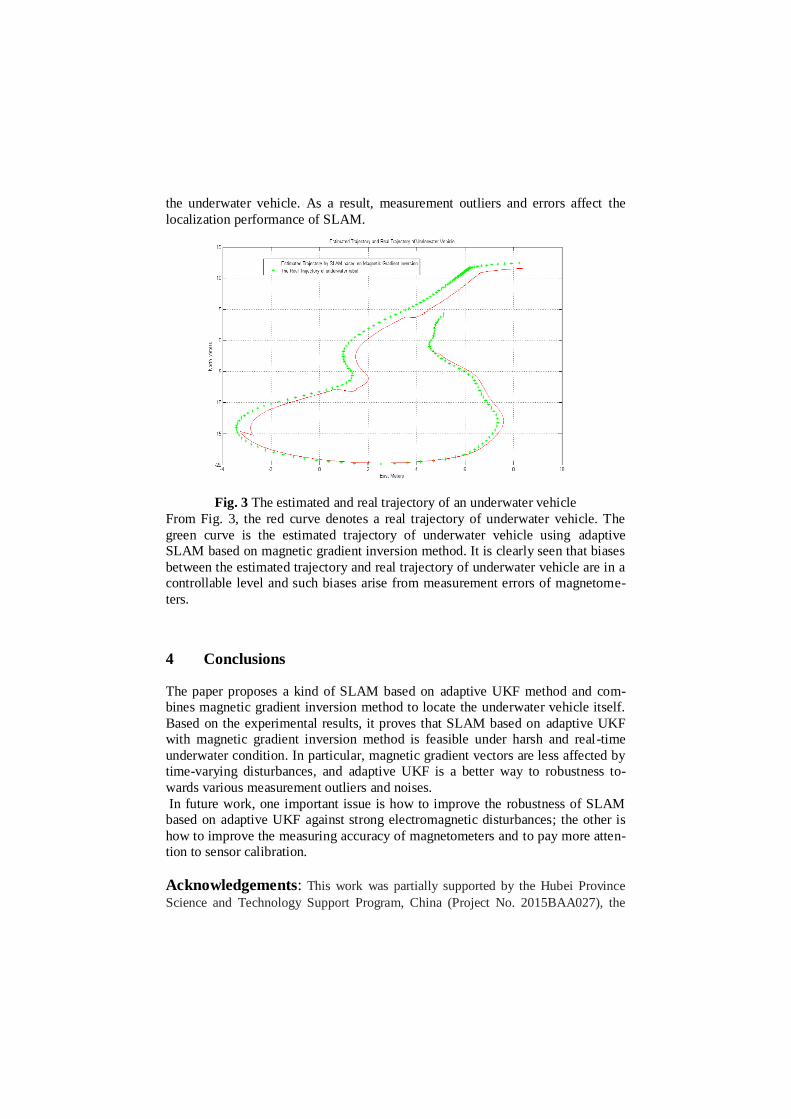
the underwater vehicle. As a result, measurement outliers and errors affect the

localization performance of SLAM.

Fig. 3 The estimated and real trajectory of an underwater vehicle

From Fig. 3, the red curve denotes a real trajectory of underwater vehicle. The

green curve is the estimated trajectory of underwater vehicle using adaptive

SLAM based on magnetic gradient inversion method. It is clearly seen that biases

between the estimated trajectory and real trajectory of underwater vehicle are in a

controllable level and such biases arise from measurement errors of magnetome-

ters.

4 Conclusions

The paper proposes a kind of SLAM based on adaptive UKF method and com-

bines magnetic gradient inversion method to locate the underwater vehicle itself.

Based on the experimental results, it proves that SLAM based on adaptive UKF

with magnetic gradient inversion method is feasible under harsh and real-time

underwater condition. In particular, magnetic gradient vectors are less affected by

time-varying disturbances, and adaptive UKF is a better way to robustness to-

wards various measurement outliers and noises.

In future work, one important issue is how to improve the robustness of SLAM

based on adaptive UKF against strong electromagnetic disturbances; the other is

how to improve the measuring accuracy of magnetometers and to pay more atten-

tion to sensor calibration.

Acknowledgements: This work was partially supported by the Hubei Province

Science and Technology Support Program, China (Project No. 2015BAA027), the

Jiangsu Province Science and Technology Support Program, China (Project No.

BE2014866), and the South Wisdom Valley Innovative Research Team Program.

Reference

1. H. Durrant-Whyte and T. Bailey, “Simultaneous localization and mapping (SLAM): part I,”

IEEE Robotics and Automation Magazine, vol. 13, no. 2, 99-108 (2006).

2. T. Bailey and H. Durrant-Whyte, “Simultaneous localization and mapping (SLAM): part II,”

IEEE Robotics and Automation Magazine, vol. 13, no. 3, 108-117 (2006).

3.Wang Fei, Cui Jin-Qiang, Chen Ben-Mei, Lee Tong H, “A Comprehensive UAV Indoor Navi-

gation System Based on Vision Optical Flow and Laser Fast SLAM.” ACTA AUTOMATICA

SINICA, Vol.39, No.11, 1890-1900 (2013).

4. R. Sim, P. Elinas, M. Griffin, and J.J. Little, “Vision-based SLAM using the Rao-

Blackwellised particle filter”, In IJCAI Workshop on Reasoning with Uncertainty in Vehicleics

(RUR), 2005.

5. A.J. Davision, I. Reid, N. Molton, and O. Stasse, “MonSLAM: Real-time single camera

SLAM”, IEEE Transactions on Pattern Analysis and Machine Intelligence, vol. 29, No.6, 1052-

1067 (2007).

6. A. Davison, “Real-time simultaneous localization and mapping with a single camera.” in

Proc. International Conference on Computer Vision, Nice, (2003).

7. T. Bailey, “Constraint initialization for bearing only slam,” IEEE Int. Conf. on Vehicleics and

Automation, ICRA, Taipei, Taiwan, 1966-1971 (2005).

8. Sunhyo Kim and Se-Young Oh, “Slam in indoor environments using omni-directional vertic-

al and horizontal line features”, Journal of Intelligent and Vehicleics Systems, vol.51, no.1, 31-

43 (2008).

9. Young-Ho Choi and Se-Young Oh, “Grid-based visual slam in complex environments”,

Journal of Intelligent and Vehicleics Systems, vol. 50, no.3, 241-255(2007).

10. Zheng, H., Wang, H., Wu, L., Chai, H., Wang, Y. “Simulation Research on Gravity-

Geomagnetism Combined Aided Underwater Navigation,” Royal Institute of Navigation, vol.

66, No. 1, 83-98 (2013).

11. Wu, L., Tian, X., Ma, H. and Tian, J.W, “Underwater Object Detection Based on Gravity

Gradient,” IEEE Geoscience and Remote Sensing Letters, Vol. 7, No. 2, 362-365 (2010).

12. Liu Ming, Wang Hai-Jun, Jiang Yan-Song, “System Modeling of SLAM-based

Geomagnetic Aided Inertial Navigation,” Aviation Precision Manufacturing Technology, vol.

47, No. 6, 13-16 (2011).

13. Shi-cheng Wang, da-wei Sun, Jin-Sheng, Zhang, Li-hua, Chen, “Research on Geomagnet-

ism Navigation and Localization Based on SLAM,” Fire Control & Command Control, vol. 35,

no.12, 35-37 (2010).

14.Lin Wu, Xin Tian and Jie Ma et al, “Underwater Object Detection Based on Gravity Gra-

dient,” IEEE Geoscience and Remote Sensing Letters, vol. 7, no.20, 362-365 (2010).

15. S. Julier, J. Uhlmann, and H. F. Durrant-Whyte, “A new method for the nonlinear transfor-

mation of means and covariance in filters and estimators,” IEEE Transactions on Automatic

Control, vol. 45, no.3, 477-482 (2000).

16. S.J. Julier and J.K. Uhlmann, “Unscented filtering and nonlinear estimation,” Proceedings

of the IEEE, vol. 92, no.3, 401-422 (2004).

17. Yu Huang, Li-Hua Wu, and Feng Sun “Underwater Continuous Localization Based on

Magnetic Dipole Target Using Magnetic Gradient Tensor and Draft Depth, “IEEE Geosci.

Remote Sens.Lett.vol.11,no.1, 178-180 (2014).

18. Hao yan-ling, Zhao ya-feng, Hu jun-feng “Preliminary analysis on the application of geo-

magnetic field matching in underwater vehicle navigation, “Progress in Geophysics. Vol.18, 64-

67 (2008).

19. Yu Huang, Sun Feng, Hao Yan-ling “Simplest magnetometer configuration scheme to

measure magnetic field gradient tensor, “Proceedings of the 2010 IEEE International Confe-

rence on Mechatronics and Automation. Vol.5, 1426-1430 (2010).