Adaptive Range Oversampling to Achieve Faster Scanning on

Adaptive Range Oversampling to Achieve Faster Scanning on the National WeatherRadar Testbed Phased-Array Radar

CHRISTOPHER D. CURTIS AND SEBASTIAN M. TORRES

Cooperative Institute for Mesoscale Meteorological Studies, University of Oklahoma, and

NOAA/OAR/National Severe Storms Laboratory, Norman, Oklahoma

(Manuscript received 7 December 2010, in final form 8 July 2011)

ABSTRACT

This paper describes a real-time implementation of adaptive range oversampling processing on the Na-

tional Weather Radar Testbed phased-array radar. It is demonstrated that, compared to conventional

matched-filter processing, range oversampling can be used to reduce scan update times by a factor of 2 while

producing meteorological data with similar quality. Adaptive range oversampling uses moment-specific

transformations to minimize the variance of meteorological variable estimates. An efficient algorithm is in-

troduced that allows for seamless integration with other signal processing functions and reduces the com-

putational burden. Through signal processing, a new dimension is added to the traditional trade-off triangle

that includes the variance of estimates, spatial coverage, and update time. That is, by trading an increase in

computational complexity, data with higher temporal resolution can be collected and the variance of esti-

mates can be improved without affecting the spatial coverage.

1. Introduction

Range oversampling followed with a whitening (or

decorrelation) transformation was originally developed

(Torres 2001) with the goal of improving the precision of

spectral moment and polarimetric variable estimates on

pulsed Doppler weather radars. Range oversampling

provides more samples for the estimation of meteorolog-

ical variables; these samples can be transformed (de-

correlated) and efficiently used to reduce the variance of

estimates and/or reduce the required observation times

(dwell times). Theoretical and simulation studies dem-

onstrating the advantages of these techniques (Torres

and Zrnic 2003a,b) have been successfully verified on

weather data collected with experimental setups and

offline signal processing (Ivic et al. 2003b; Torres and Ivic

2005; Choudhury and Chandrasekar 2007; Hefner and

Chandrasekar 2008). However, a real-time implemen-

tation of range oversampling processing on weather ra-

dars has not been reported to date. Although appealing,

a real-time implementation of range oversampling pro-

cessing may be feasible only on signal processing systems

based on modern hardware because of the significantly

higher demand for computational power. In this work, we

report on a recent real-time implementation of range

oversampling techniques that is computationally efficient

and leads to faster collection times with little or no sac-

rifice in data quality.

The need for faster collection times to improve the

depiction and understanding of fast-evolving hazardous

weather phenomena using radar was recognized over

three decades ago (e.g., Miller and Kropfli 1980; Carbone

et al. 1985) and has inspired many radar research and

demonstration projects (e.g., Wilson et al. 1984; Lin et al.

1986; Qiu and Xu 1996; Wurman 2002; Bluestein and

Wakimoto 2003; Zrnic et al. 2007; Heinselman et al. 2008;

McLaughlin et al. 2009; Bluestein et al. 2010; Kumjian

et al. 2010; Yussouf and Stensrud 2010). Since 2004,

scientists at the National Severe Storms Laboratory

(NSSL) have been exploring the high-temporal-resolution

weather-scanning capabilities of a 10-cm-wavelength,

agile-beam, phased-array radar. Located in Norman,

Oklahoma, this system is referred to as the National

Weather Radar Testbed (NWRT). The interested reader

is referred to Zrnic et al. (2007) and Heinselman and

Torres (2011) for in-depth technical descriptions of the

NWRT hardware and software, respectively. The NWRT

is part of the broader multifunction phased-array radar

(MPAR) initiative where the use of a single radar system

to perform both weather and aircraft surveillance functions

Corresponding author address: Christopher Curtis, 120 David

L. Boren Blvd., National Weather Center, Norman, OK 73072.

E-mail: [email protected]

VOLUME 28 J O U R N A L O F A T M O S P H E R I C A N D O C E A N I C T E C H N O L O G Y DECEMBER 2011

DOI: 10.1175/JTECH-D-10-05042.1

� 2011 American Meteorological Society 1581Unauthenticated | Downloaded 03/15/22 01:46 AM UTC

is being investigated (Weber et al. 2007; National

Academies Press 2008).

A key capability of phased-array radar technology

is the high-temporal-resolution sampling that can be

achieved through electronic beam steering. Electronic

beam steering enables focused observations of different

volumetric regions without the delays that are typically

associated with mechanically scanned radar beams.

However, electronic beam steering does not solve the

fundamental scanning trade-off between spatial sampling,

update time, and estimate variance.1 It is through signal

processing that range oversampling techniques add a new

dimension to this fundamental trade-off. That is, range

oversampling can be exploited to reduce dwell times (i.e.,

faster scanning) without degrading the variance or spatial

coverage of meteorological variable estimates.

Even though range oversampling techniques are suitable

for radars with reflector antennas, such as the Weather

Surveillance Radar-1988 Doppler (WSR-88D), electron-

ically steered phased-array radars are an ideal platform

for operational implementation. This is particularly true

if the goal is to reduce update times because phased-

array radars have no beam smearing or mechanical in-

ertia; thus, they impose no limitations on the radar beam

scanning speed. The NWRT obviously meets these crite-

ria, and its digital receiver collects range-oversampled data

by default (i.e., it samples at a 60-m spacing with a 240-m

pulse). Additionally, the NWRT signal processing cluster

is a distributed computing platform, which has more than

enough computational power to handle the additional

complexity demanded by range oversampling processing.

Motivated by the need for high-temporal resolution

data, range oversampling has been running operationally

on the NWRT since the spring of 2010. An adaptive al-

gorithm was designed to select processing transfor-

mations that lead to lower variances of meteorological

variable estimates for varying conditions. The algorithm

was tailored for efficiency to ensure compatibility with

other required signal processing functions and to mini-

mize the increased requirements for computational

power. The real-time implementation of adaptive range

oversampling, which is the focus of this work, has led to

further reductions of scan update times (up to 2 times)

on the NWRT with little or no loss of data quality.

The rest of the paper is organized as follows. Section 2

reviews the theory behind range oversampling process-

ing and motivates the need for an adaptive algorithm.

Section 3 describes the real-time implementation of

adaptive range oversampling processing on the NWRT.

Specifically addressed are the increased computational

complexity and the interaction with other signal processing

functions. The final section describes the modification of

scanning strategies that led to a reduction of update times

by exploiting range oversampling processing. The per-

formance improvements are illustrated on weather data

collected with the NWRT.

2. The path to adaptive pseudowhitening

Whereas conventional sampling of weather radar

signals (V) occurs at a rate of t21, where t is the duration

of the transmitted pulse, range oversampling by a factor

of L entails acquiring time series data at increased rates

so that L complex samples are collected during the time

t. Thus, range oversampling provides more samples with-

out increasing the dwell time. As mentioned before,

oversampling in range is feasible with modern commercial

single-board digital receivers (Ivic et al. 2003a). For ex-

ample, oversampled data are readily available on radar

systems that employ software-based digital matched filters,

such as the NWRT. On systems that rely on hardware-

based digital matched filters, such as the WSR-88D, the

hardware has to be reprogrammed to provide oversampled

data. Two methods for processing range-oversampled sig-

nals are described next: conventional digital matched-filter

processing and range oversampling processing. The sec-

tion on range oversampling processing is further divided

to show the progression from the whitening transfor-

mation to the currently implemented adaptive pseudo-

whitening approach.

a. Digital matched-filter processing

A digital matched filter performs coherent averaging

of the range-oversampled data from which autocovar-

iances are estimated. Herein, meteorological variable

estimates obtained from these autocovariances are re-

ferred to as matched-filter-based (MFB) estimates. For

an M-pulse dwell and given range resolution cell the

corresponding M matched-filtered samples y are ob-

tained as

y 5 hV, (1)

where h is the 1 3 L digital matched-filter vector, and V

is the L 3 M complex-valued matrix of oversampled

time series data. For convenience, we express V 5

(V0, V

1, . . . , V

M21), where Vm are L 3 1 column vectors of

range-oversampled signals at sample time m (m 5 0,

1, . . . , M 2 1). That is, Vm

5 [V(0, m), V(1, m), . . . ,V(L 2

1, m)]T, where the superscript T denotes matrix

1 Beam multiplexing (Yu et al. 2007) is purposely ignored in this

discussion because its complex sampling renders it incompatible

with other signal processing techniques, such as traditional ground

clutter filtering.

1582 J O U R N A L O F A T M O S P H E R I C A N D O C E A N I C T E C H N O L O G Y VOLUME 28

Unauthenticated | Downloaded 03/15/22 01:46 AM UTC

transposition, and V(l, m) is the signal at the over-

sampled range index l (l 5 0, 1, . . . , L 2 1) and sample

time m. The digital matched filter that maximizes the

signal-to-noise ratio (SNR) of the random signal V is

given by the eigenvector corresponding to the largest

eigenvalue of the normalized range correlation matrix

CV(Chiuppesi et al. 1980). The normalized range–

correlation matrix can be obtained from the modified

pulse, which depends on the transmitter pulse envelope and

the receiver impulse response (Torres and Zrnic 2003a).

b. Range oversampling processing

In contrast to the digital matched filter, range over-

sampling processing performs incoherent averaging of

transformed range-oversampled data. Transformed sam-

ples are used to compute autocovariance estimates for

each oversampled range gate (there are L range gates in

each range resolution cell). These autocovariances are

averaged in blocks of L estimates from which the me-

teorological variables are computed. Transformed over-

sampled signals at a given range resolution cell are

obtained as

X 5 WV, (2)

where W is the transformation matrix and X is the

transformed time series matrix with the same structure

as V. In general, W can be any L 3 L complex-valued

matrix that satisfies the ‘‘power-preserving criterion’’

tr(W*CVWT) 5 L, (3)

where tr(�) is the matrix trace operation, the superscript

* denotes complex conjugation, and CV

is the normal-

ized range–correlation matrix.

Estimates obtained from range oversampling process-

ing exhibit lower variances than their MFB counterparts,

particularly at high SNR. The variance reduction fac-

tor (VRF), defined as the ratio of MFB and range over-

sampling estimate variances, is useful to quantify the

performance of different range oversampling processing

transformations. Its value at high SNR, which is denoted

by VRF‘, represents the performance of an oversampling

processing transformation in a noise-free environment.

1) WHITENING TRANSFORMATION

A special case of W is the whitening transformation

(Torres and Zrnic 2003a) given by W 5 H21, where H is

the matrix square root of CV , that is, CV 5 H*HT. Herein,

meteorological variable estimates obtained from whit-

ened signals are referred to as whitening transformation–

based (WTB) estimates. It can be demonstrated that a

whitening transformation produces the maximum VRF‘

(Torres and Zrnic 2003a). However, a whitening trans-

formation also increases the noise power in the trans-

formed oversampled signal because the noise becomes

colored.

The noise-enhancement factor (NEF) is defined as the

ratio of the post- to pretransformation noise powers, and

it can be expressed in terms of the transformation matrix

as [cf. (12) of Torres and Zrnic 2003a]

NEF 5 tr(W*WT)/L. (4)

The large noise-enhancement factor of the whitening

transformation is its main drawback; at low SNR, WTB

estimates exhibit larger variances than their MFB coun-

terparts. This effect can be quantified in a more mean-

ingful way by the crossover SNR (SNRc), which is defined

as the SNR at which the variance of estimates obtained

with range oversampling and digital matched-filter pro-

cessing are the same (Torres and Zrnic 2003a). Only at

SNRs above SNRc do estimates from range oversampling

processing have a lower variance than those from matched-

filter processing.

The effectiveness of range oversampling transforma-

tions below and above the SNRc suggests a straightfor-

ward means to mitigate noise enhancement effects. As

suggested by Torres and Zrnic (2003a), a simple adap-

tive technique can use an estimate of the SNR to select

the better processing option based on a priori knowl-

edge of SNRc. That is, range oversampling processing is

used at SNRs above SNRc, and matched-filtering pro-

cessing otherwise. Hence, the higher the SNRc, the nar-

rower the range of SNRs for which range oversampling

processing adds any value.

2) FIXED PSEUDOWHITENING TRANSFORMATION

As mentioned before, WTB processing achieves max-

imum variance reduction at high SNR but results in the

largest noise enhancement, that is, the highest SNRc.

Unfortunately, if using the simple adaptive algorithm based

on SNRc described above, then the range of effectiveness

for whitening is limited. To mitigate this limitation, pseu-

dowhitening (or partial whitening) transformations were

recommended by Torres et al. (2004a) as a means to trade

less noise enhancement (i.e., a lower SNRc) for a smaller

variance reduction factor at high SNR.

In the general framework of pseudowhitening pro-

cessing, the transformation matrix is defined as (Torres

et al. 2004a)

W 5 gSþP*T, (5)

where g is the transformation gain, S1 is a diagonal real-

valued matrix, and P is a unitary matrix from the singular

DECEMBER 2011 C U R T I S A N D T O R R E S 1583


value decomposition (SVD) of H (defined above as the

matrix square root of CV

). From the SVD of H,

H 5 PSQ*T, P and Q are unitary matrices and S is a di-

agonal matrix with the singular values of H, sl (l 5 0,

1, . . . , L 2 1). The transformation gain g can be calcu-

lated in terms of S and S1 in order to satisfy (3) [see Eq.

(16) in Torres et al. 2004a] as

g 5

ffiffiffiffiffiffiffiffiffiffiffiffiffiffiffiffiffiffiffiffiffiffiffiffiffiL

tr[(S1)2S2]

s. (6)

The nonzero entries of S1 along its main diagonal s1l

determine the type of pseudowhitening transformation.

For example, W in (5) becomes a whitening trans-

formation if s1l 5 s21

l . Alternatively, pseudowhitening

with a ‘‘sharpening’’ filter is obtained when s1l 5

sl[as2l 1 (1 2 a)]21, where a is the sharpening parame-

ter that controls the degree of pseudowhitening (Torres

et al. 2004a). As a varies from 0 to 1, W ranges from nearly

equivalent to a matched filter to a whitening trans-

formation. Herein, meteorological variables obtained us-

ing a fixed pseudowhitening transformation are referred

to as pseudowhitening transformation–based (PTB) es-

timates. With this formulation, the NEF defined in (4)

becomes

NEF 5g2

Ltr[(S1)2]. (7)

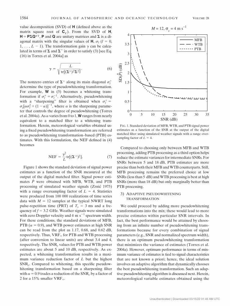
Figure 1 shows the standard deviation of signal power

estimates as a function of the SNR measured at the

output of the digital matched filter. Signal power esti-

mates P were obtained with MFB, WTB, and PTB

processing of simulated weather signals (Zrnic 1975)

with a range oversampling factor of L 5 4. Statistics

were produced from 100 000 realizations of time series

data with M 5 12 samples at the typical NWRT long

pulse-repetition time (PRT) of Ts 5 3 ms and a fre-

quency of f 5 3.2 GHz. Weather signals were simulated

with zero Doppler velocity and 4 m s21 spectrum width.

For these conditions, the standard deviations of MFB,

PTB (a 5 0.9), and WTB power estimates at high SNR

can be read from the plot as 1.17, 0.68, and 0.62 dB,

respectively. Thus, VRF‘ for PTB and WTB processing

(after conversion to linear units) are about 3.4 and 4,

respectively. The SNRc values for PTB and WTB power

estimates are about 5 and 10 dB, respectively. As ex-

pected, a whitening transformation results in a maxi-

mum variance reduction factor of L but the highest

SNRc. Compared to whitening, this specific pseudow-

hitening transformation based on a sharpening filter

with a 5 0.9 trades a reduction of the SNRc by a factor of

2 for a 15% smaller VRF‘.

Compared to choosing only between MFB and WTB

processing, adding PTB processing as a third option helps

reduce the estimate variances for intermediate SNRs. For

SNRs between 5 and 18 dB, PTB estimates are more

precise than both their MFB and WTB counterparts. Still,

MFB processing remains the preferred choice at low

SNRs (less than 5 dB) and WTB processing is best at high

SNRs (more than 18 dB) but only marginally better than

PTB processing.

3) ADAPTIVE PSEUDOWHITENING

TRANSFORMATION

We could proceed by adding more pseudowhitening

transformations into the mix; these would lead to more

precise estimates within particular SNR intervals. In

fact, the best performance would be attained by choos-

ing from an infinite number of pseudowhitening trans-

formations because for every combination of signal

parameters (e.g., SNR and normalized spectrum width),

there is an optimum pseudowhitening transformation

that minimizes the variance of estimates (Torres et al.

2004a). However, optimum performance in terms of min-

imum variance of estimates is tied to signal characteristics

that are not known a priori; hence, the ideal solution

involves an adaptive algorithm that dynamically chooses

the best pseudowhitening transformation. Such an adap-

tive pseudowhitening algorithm is discussed next. Herein,

meteorological variable estimates obtained using the

FIG. 1. Standard deviation of MFB, WTB, and PTB signal power

estimates as a function of the SNR at the output of the digital

matched filter using simulated weather signals with a range over-

sampling factor of L 5 4.



optimum and adaptive pseudowhitening transfor-

mations are referred to as optimum pseudowhitening

transformation–based (OPTB) and adaptive pseudo-

whitening transformation–based (APTB) estimates, re-

spectively.

The adaptive pseudowhitening algorithm starts with

the previously mentioned optimum pseudowhitening

transformation that minimizes the variance of meteo-

rological variable estimates. An expression for the var-

iance of the estimator of a particular spectral moment u

can be computed using Eq. (28) from Torres et al.

(2004a),

Var(u) 5 D[Atr(C2X

S) 1 Btr(CX

S

CXN

) 1 Ctr(C2X

N)],

(8)

where A, B, C, and D are moment-specific constants that

depend on the SNR at the output of the digital receiver

(SNR0) and the normalized spectrum width (svn). The

CXS

and CXN

matrices are normalized range–correlation

matrices of the transformed signal, and noise compo-

nents of CV and can be computed in terms of W and H

as CXS5 W*CVWT 5 W*H*HTWT and CXN

5 W*WT

(Torres et al. 2004a). This assumes that the signal and

noise components of V are uncorrelated and the noise is

white. On the NWRT, signal power (S), mean Doppler

velocity (y), and spectrum width (sy) are estimated using

classical autocovariance processing based on lag-0 and

lag-1 autocovariance estimates (Doviak and Zrnic 1993).

The variance expression in (8) is exact for the signal power,

but is an approximation based on perturbation analyses for

the Doppler velocity and spectrum width (Torres and

Zrnic 2003b). For these variables, the approximations

should be sufficiently accurate even though the resulting

transformation may be slightly suboptimal. The values of

the constants A, B, C, and D are given in Table 1 for the

three previously mentioned spectral moment estimators.

To find the optimal pseudowhitening transformation

for a particular variable, the variance expression in (8) is

minimized as described in Torres et al. (2004a). This

leads to an expression for the transformation [cf. (32) in

Torres et al. 2004a] given in terms of the s1l by

s1l 5

slffiffiffiffiffiffiffiffiffiffiffiffiffiffiffiffiffiffiffiffiffiffiffiffiffiffiffiffiffiffiffiffiffiffiffiffiAs4

l 1 Bs2l 1 C

q , (9)

where sl are the singular values of H. Note that the

scaling factor D at the beginning of the generalized var-

iance expression does not appear in the expression for the

optimum pseudowhitening transformation. The optimum

pseudowhitening transformation is only optimum when

SNR and svn are known exactly, but these values are not

known a priori. In contrast, adaptive pseudowhitening

uses estimates of SNR0 and svn to find moment-specific

values of A, B, and C needed in (9). We will show that this

leads to a nearly optimal transformation that can be im-

plemented in real time.

The first step in adaptive pseudowhitening is to estimate

SNR0 and svn. For a straightforward implementation,

MFB estimates of SNR0 and svn are computed from

matched-filtered samples using the digital matched filter

in (1). Because different estimates may be obtained for

different range resolution cells, and (9) is specific to each

meteorological variable, a new transformation needs to be

computed for each spectral moment and each range res-

olution cell. That is, the MFB estimates of SNR0 and svn

are used to calculate moment-specific values of A, B, and

C, which are substituted into (9) to find S1. Then, at each

range resolution cell, a moment-specific transformation W

is formed using (5). Finally, a transformed signal matrix X

is computed for each meteorological variable, which can

be used to produce estimates.

Figure 2 illustrates the performance of APTB estimates

of signal power compared to MFB, WTB, PTB, and

OPTB estimates as a function of the MFB SNR using

100 000 realizations of simulated weather signals with

a range oversampling factor of L 5 4. OPTB estimates

are included as a reference; they are only available in

a simulation environment because they depend on the

precise knowledge of signal parameters. Both plots use

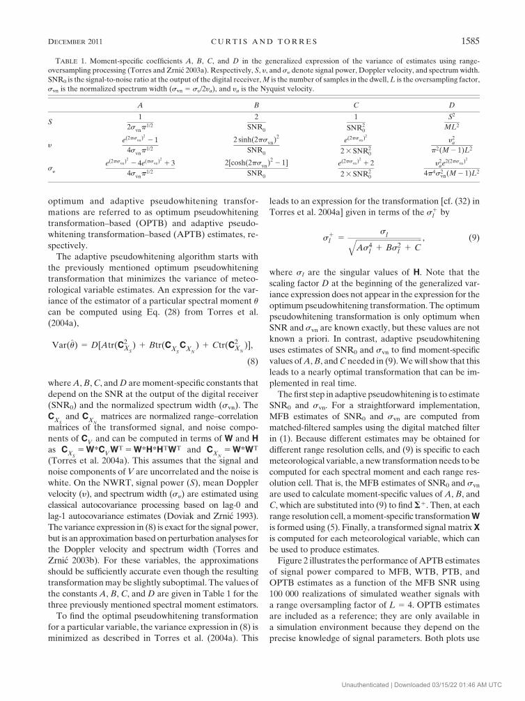
TABLE 1. Moment-specific coefficients A, B, C, and D in the generalized expression of the variance of estimates using range-

oversampling processing (Torres and Zrnic 2003a). Respectively, S, y, and sy denote signal power, Doppler velocity, and spectrum width.

SNR0 is the signal-to-noise ratio at the output of the digital receiver, M is the number of samples in the dwell, L is the oversampling factor,

svn is the normalized spectrum width (svn 5 sy/2ya), and ya is the Nyquist velocity.

A B C D

S1

2svnp1/2

2

SNR0

1

SNR20

S2

ML2

ye(2psvn)2

2 1

4svn

p1/2

2 sinh(2psvn)2

SNR0

e(2psvn)2

2 3 SNR20

y2a

p2(M 2 1)L2

sy

e(2psvn)2

2 4e(psvn)2

1 3

4svnp1/2

2[cosh(2psvn

)22 1]

SNR0

e(2psvn)2

1 2

2 3 SNR20

y2ae2(2psvn)2

4p4s2vn(M 2 1)L2



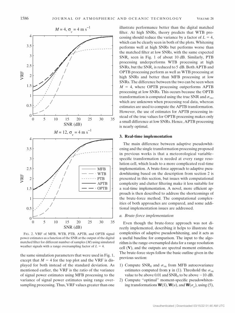
the same simulation parameters that were used in Fig. 1,

except that M 5 4 for the top plot and the VRF is dis-

played for both instead of the standard deviation. As

mentioned earlier, the VRF is the ratio of the variance

of signal power estimates using MFB processing to the

variance of signal power estimates using range over-

sampling processing. Thus, VRF values greater than one

illustrate performance better than the digital matched

filter. At high SNRs, theory predicts that WTB pro-

cessing should reduce the variance by a factor of L 5 4,

which can be clearly seen in both of the plots. Whitening

performs well at high SNRs but performs worse than

the matched filter at low SNRs, with the same expected

SNRc seen in Fig. 1 of about 10 dB. Similarly, PTB

processing underperforms WTB processing at high

SNRs, but the SNRc is reduced to 5 dB. Both APTB and

OPTB processing perform as well as WTB processing at

high SNRs and better than MFB processing at low

SNRs. The difference between the two can be seen when

M 5 4, where OPTB processing outperforms APTB

processing at low SNRs. This occurs because the OPTB

transformation is computed using the true SNR and svn,

which are unknown when processing real data, whereas

estimates are used to compute the APTB transformation.

However, the use of estimates for APTB processing in-

stead of the true values for OPTB processing makes only

a small difference at low SNRs. Hence, APTB processing

is nearly optimal.

3. Real-time implementation

The main difference between adaptive pseudowhit-

ening and the single transformation processing proposed

in previous works is that a meteorological variable–

specific transformation is needed at every range reso-

lution cell, which leads to a more complicated real-time

implementation. A brute-force approach to adaptive pseu-

dowhitening based on the description from section 2 is

presented in this section, but issues with computational

complexity and clutter filtering make it less suitable for

a real-time implementation. A novel, more efficient ap-

proach is then described to address the shortcomings of

the brute-force method. The computational complex-

ities of both approaches are compared, and some addi-

tional implementation issues are addressed.

a. Brute-force implementation

Even though the brute-force approach was not di-

rectly implemented, describing it helps to illustrate the

complexities of adaptive pseudowhitening, and it acts as

a useful baseline for comparison. The input to the algo-

rithm is the range-oversampled data for a range resolution

cell (V), and the outputs are spectral moment estimates.

The brute-force steps follow the basic outline given in the

previous section:

1) Compute SNR0 and svn from MFB autocovariance

estimates computed from y in (1). Threshold the svn

value to be above 0.01 and SNR0 to be above 210 dB.

2) Compute ‘‘optimal’’ moment-specific pseudowhiten-

ing transformations W(S), W(y), and W(sy), using (5),

FIG. 2. VRF of MFB, WTB, PTB, APTB, and OPTB signal

power estimates as a function of the SNR at the output of the digital

matched filter for different number of samples (M) using simulated

weather signals with a range oversampling factor of L 5 4.



(6), and (9) for power, velocity, and spectrum width

estimates, respectively, where W(u) denotes the trans-

formation specific to the spectral moment u [as de-

fined in (8)].

3) Transform the original time series matrix V using the

computed moment-specific transformations to produce

time series matrices X(S), X(y), and X(sy) using (2).

4) For each required lag-k autocovariance estimate,

compute L range-oversampled moment-specific au-

tocovariances from the corresponding transformed

time series matrices R(l)

X(u)(k) 5 (M 2 jkj)21�M2jkj21

m50

X*(u)(l, m)X(u)(l, m 1 k). Required autocovarian-

ces are lag 0 from X(S) for power, lag 1 from X(y)

for velocity, and lags 0 and 1 from X(sy) for spectrum

width.

5) Compute the required autocovariance estimates

RX(S)

(0), RX(y)

(1), RX(s

y)(0), and R

X(sy)(1) by aver-

aging the corresponding L range-oversampled auto-

covariance estimates from step 4.

6) Compute APTB moment estimates from the spectral

moment–specific averaged autocovariances.

The first step adds more computational complexity be-

cause MFB data need to be produced from V using a digital

matched filter as described in (1). The thresholding of svn is

necessary to avoid an increase in the variance of all APTB

estimators resulting from the large errors of the spectrum

width estimator at very narrow spectrum widths. Similarly,

thresholding SNR0 avoids issues with unreasonably small

SNR0 values because of estimation error.

The key part of the brute-force approach that in-

creases computational complexity is step 3. There is a

direct computational effect from having a separate ma-

trix of time series data for each meteorological variable

and indirect effects associated with ground clutter fil-

tering and other ancillary signal processing functions. It

is these indirect effects that may be the most costly be-

cause, in some cases, ground clutter filtering could use

more floating point operations than all of the other

processing steps combined. The major problem is that

the brute-force approach can lead to ground clutter fil-

tering of all three matrices of transformed time series

data and the MFB data instead of only filtering V. An

alternative is to use a ground clutter filter that outputs

a filtered version of V that can then be transformed with

moment-specific transformations. This would require

either additional computations when using frequency-

domain filters2 or the use of time-domain filters, which

may not always be feasible. The preferred approach is to

find a way to transform V in such a way that ground

clutter filtering only needs to be applied once and any

type of filter can be used.

b. Efficient implementation

The novel idea that leads to an efficient real-time im-

plementation is to split up the transformation into two

distinct steps. From (5), the first step is the unitary matrix

given by P*T, and the second step is a weighting made up

of the gain g and the diagonal matrix S1. The unitary

matrix is the same for all of the transformations, so V can

be multiplied by P*T to give a common partially trans-

formed time series matrix ~X 5 P*TV. The weighting gS1

can then be computed for each meteorological variable

and applied separately. If this weighting were applied to

the partially transformed time series data, the ground

clutter filter would still need to produce a moment-

specific filtered version of the time series matrix ~X sim-

ilar to the brute-force approach. The alternative is to

apply the weighting step to the autocovariances; this al-

lows nearly any type of filter to be used, including those

that produce filtered autocovariances from the Doppler

spectrum instead of filtered time series data. That is, the

lag-k autocovariance estimate RX

(k) from fully trans-

formed data can be computed as the weighted average of

the L lag-k autocovariance estimates R(l)~X (k) from par-

tially transformed data,

RX(k) 5 �L21

l50dlR

(l)~X (k), (10)

where d 5 (d0, d1, . . . , dL21) is the length L weight vector.

A derivation of the equivalence between the two-step

efficient implementation and the brute-force approach

given in (10) and the relationship between d and gS1 can

be found in appendix A.

In addition to the advantages for computing the re-

quired autocovariances, the two-step application of the

moment-specific adaptive pseudowhitening transforma-

tion allows the ground clutter filter to be applied only

once, and any filter can be used, including those that

produce filtered autocovariances. A further benefit of the

efficient implementation concerns matched-filtered data.

Both approaches need matched-filtered data in order to

estimate SNR0 and svn, but for the efficient implemen-

tation, the matched-filtered data are already provided as

one of the autocovariances computed from the partially

transformed data. This will be explored in more detail as

the steps for the efficient implementation are described.

The steps for the efficient implementation are similar

to the brute-force approach, but additional improvements

simplify the algorithm. For example, with the efficient

2 In this scenario, conversion back to the time domain after the

application of a frequency-domain filter would require L additional

Fourier transforms and a way to reconstruct the missing infor-

mation from the filtered spectral components.



implementation, the two-step process for computing W

using a Cholesky decomposition and an SVD is replaced

with a single eigendecomposition. The efficient imple-

mentation starts from the normalized range–correlation

matrix CV . An eigendecomposition of the Hermitian ma-

trix CV is utilized such that CV 5 U*LUT, where U is the

matrix of eigenvectors and L is the diagonal matrix of ei-

genvalues with l0 $ l1 $ � � � $ lL21 $ 0. From the

Cholesky decomposition of CV

5 H*HT and the singular

value decomposition of H 5 PSQ*T, it can easily be

shown that U is equal to P (up to multiplication by unit

length complex scalars), and also that L 5 S2. Next, the

elements of the weight vector d can be obtained directly

from the eigenvalues of CV . As shown in appendix A,

dl 5 gl1l , where g is a power-preserving factor and l1

l

are the diagonal entries of L15 (S1)2. Based on the

expression for s1l given in (9), l1

l can be computed as

l1l 5 (sl

1 )25

ll

Al2l 1 Bll 1 C

, (11)

where the moment-specific A, B, and C values depend

on the estimates of SNR0 and svn computed from the

matched-filtered autocovariances. The power-preserving

factor g can then be computed using the eigenvalues and

the equation for g given in (6) as

g 5g2

L5 [tr(L1L)]21 5 �

L

l51ll

1 ll

0@

1A21

. (12)

From these expressions, the moment-specific weight

vectors d(S), d(y), and d(sy) can be obtained. The last

step is to show how the matched-filtered covariances can

be computed.

The digital matched filter was described in section 2

as a scaled version of the eigenvector corresponding

to the maximum eigenvalue of the normalized range–

correlation matrix CV . The U (or P) matrix contains the

eigenvectors, and the first eigenvector corresponds to

the largest eigenvalue. Thus, the first row of ~X is the un-

scaled matched-filtered time series data. If the L auto-

covariances are computed from ~X, then R(0)~X (k) (obtained

from the first row of ~X) is the unscaled, lag-k, matched-

filtered autocovariance. The proper scaling factor can be

found by treating the matched filter as a pseudowhitening

transformation, such that the first row of the transformed

data X is y from (1) and the other rows are zeros. This is

equivalent to selecting a transformation matrix with

s10 5 1 and s1

l 5 0 for l 5 1, 2, . . . , L 2 1. With this setup

and using the fact that l1l 5 (s l

1)2, it is easy to see from

(12) that the only nonzero element of the weight vector

d is d0 5 gl10 5 l21

0 ; thus, R(0)~X (k)/l0 is the appropriately

scaled matched-filtered autocovariance.

With all of the machinery in place, the steps of the ef-

ficient adaptive pseudowhitening algorithm are given next.

As with the brute-force approach, the input to the algo-

rithm is the range-oversampled data for a range resolution

cell (V), and the outputs are spectral moment estimates.

1) Compute the partially transformed matrix of time

series data ~X 5 U*TV, using the U computed from the

eigendecomposition of CV .

2) For each required lag-k autocovariance estimate,

compute L range-oversampled autocovariances

R(l)~X (k) from the partially transformed data. Required

autocovariances are lags 0 and 1 from ~X.

3) Compute the MFB estimates of SNR0 and svn from

R(0)~X (k)/l

0. Threshold the svn value to be above 0.01

and SNR0 to be above 210 dB.

4) Calculate the nearly optimum moment-specific

weight vectors d(S), d(y), and d(sy) using dl(u) 5

g(u)l1l (u), (11), and (12).

5) Compute the required autocovariance estimates RX(S)

(0), RX(y)

(1), RX(s

y)(0), and R

X(sy)(1) from R

(l)~X (0),

R(l)~X

(1), and the weight vectors from step 4 as shown in

(10).

6) Compute APTB spectral moment estimates from the

moment-specific averaged autocovariances.

The largest difference between the efficient implementa-

tion and the brute-force approach comes in the first few

steps. The data are partially transformed in step 1, and

any ground clutter filtering can be done between steps 1

and 2 instead of after the moment-specific transformations

that are used in the brute-force approach. This greatly

simplifies the ground clutter filtering process both in

terms of computational complexity and the types of fil-

ters that can be effectively utilized. In step 5, the rest of

the transformation is applied using the weight vectors

computed in step 4.

To summarize, the efficient implementation simplifies the

ground clutter filtering process and allows nearly any type

of filter to be used, which can reduce the computational

complexity significantly. The already filtered MFB data are

computed as a by-product of the partial transformation,

which is simpler than computing it separately. Our tests

show that the efficient implementation takes about 4 times

as many computations as digital matched filtering, assum-

ing L 5 4, while the brute-force implementation takes

about 12 times as many computations. This factor of 3 in

computational savings is in addition to any savings from

ground clutter filtering. A more detailed analysis of the

computational complexity can be found in appendix B.

c. Additional implementation issues

The basic steps for performing adaptive pseudowhit-

ening processing have been presented, but there are



a couple of additional issues that need to be addressed

for a complete implementation. The first is the effect of

these transformations on the noise. The algorithm shows

how the autocovariances are computed, but the appropriate

noise value needs to be subtracted from the lag-0 autoco-

variance estimate, or total power, in order to calculate the

signal power that is needed in the reflectivity computation.

The noise power needs to be adjusted using the NEF from

section 2. Although this was introduced as a noise en-

hancement factor, the factor can be less than 1 and can

increase or decrease the noise power depending on the

transformation. Based on (7) and using eigenvalues instead

of singular values, the moment-specific noise enhancement

factor NEF(u) can be computed for each weight vector as

NEF(u) 5 �L21

l50dl(u). (13)

In other words, the NEF is just the sum of the elements

of the weight vector. For the MFB case, this reduces to

a moment-independent NEF 5 l210 . For the APTB case,

the signal power can be computed as S 5 RX(S)

(0) 2

NEF(S)N, where N is the noise power at the output of

the digital receiver and NEF(S) is the signal power–specific

noise enhancement factor.

The last issue is data censoring (or thresholding). Data

censoring is a data quality issue whereby only data from

significant weather returns are utilized (e.g., displayed and

sent to algorithms) and data from noise-like returns are

not. A common way to censor weather radar data is to use

an SNR threshold. Data corresponding to signals above

a particular SNR threshold are treated as significant, and

data below the threshold are treated either as non-

significant or noise. For adaptive pseudowhitening, this is

complicated by the fact that the noise powers are different

for each range resolution cell, and the corresponding SNR

threshold should be adjusted because of the lower vari-

ance of APTB estimates. For our implementation, we

chose a simple approach and used the SNR computed

from the MFB data and a fixed threshold. This censors the

data in the same way as the matched-filter approach, but

the estimates that are designated as significant will often

have better quality than the ones computed with the MFB

data. By taking advantage of the improved estimates from

the APTB processing, it may be possible to preserve more

data that are considered significant, but this requires ad-

ditional research that is beyond the scope of this work.

4. Real data from the NWRT

In spring 2010, the adaptive pseudowhitening algorithm

described in the previous section was implemented for

real-time operation on the NWRT. The NWRT digital

signal processor is a Linux-based distributed-computing

system in which a cluster of multiple commercial off-the-

shelf dual-processor nodes (based on dual-core 3-GHz

Intel Xeon processors) communicate via a high-speed

interconnect. All signal processing functions are imple-

mented in software using the concept of processing modes

and processing blocks, which maximizes code reusability

and leads to a rapid development cycle (Heinselman and

Torres 2011). As stated in the introduction, range over-

sampling techniques can be used to reduce either the

variance of estimates or the required observation times.

In this section, we use data collected by the NWRT to

demonstrate how adaptive pseudowhitening combined

with the proper scanning strategy can achieve both

faster updates and improved data quality with no loss of

coverage. Data are processed to illustrate and compare

the performance improvement that was realized after

operational NWRT scanning strategies were modified to

use adaptive pseudowhitening.

For this example, we will use one of the scanning strat-

egies that was developed for the spring 2010 experiments

using conventional matched-filter processing and was

later modified to exploit the real-time implementation

of adaptive pseudowhitening. The scanning strategy was

designed to provide optimized sampling in elevation and

azimuth as proposed by Brown et al. (2000) for the WSR-

88D. The strategy performs a sequence of elevation scans

at 22 unique constant elevations (from 0.58 to 538). For

each elevation scan, the azimuth is step-scanned to cover

a 908 azimuthal sector with 109 beams that are spaced at

half-beamwidth increments.3 The PRTs were designed

so that their corresponding unambiguous ranges are

long enough to sample storms with heights up to 18 km

above ground level. ‘‘Split cuts’’ (Torres et al. 2004b) are

employed at the lower elevation angles (10 elevations

below 68) where long PRTs are needed to meet coverage

requirements. At each beam, data collected with a long

PRT are used to compute reflectivity estimates with no

range ambiguity, and data collected with a short PRT are

used to compute Doppler velocity and spectrum width

estimates on a larger Nyquist cointerval. These may be

ambiguous in range but are ‘‘range unfolded’’ using the

reflectivity from the long-PRT data. The number of

pulses per dwell (beam) depends on the PRT(s) at each

elevation angle and is chosen such that the data meet WSR-

88D operational standards for data quality (NOAA 2006).

For the original NWRT scanning strategy, the total number

of beams (2398) and dwell times (determined by the

3 Beam spacing as a function of beamwidth results in irregular

sampling because the beamwidth of phased-array antennas in-

creases as the beam is steered away from boresight.



specific PRTs and number of samples) provide a base-

line update time of 118.6 s for the entire sector.

On 2 April 2010, the scanning strategy described above

was used on the NWRT to sample a severe storm event

southeast of Norman. Figure 3 shows plan-position in-

dicator (PPI) displays of reflectivity (left panels) and

Doppler velocity (right panels) fields at ;1054 UTC.

Data shown in this figure correspond to the lowest ele-

vation scan at an elevation of 0.58. At this elevation, 16

samples using the long PRT (3 ms) and 64 samples using

the short PRT (0.8 ms) are collected at each range res-

olution volume. The total dwell time for each beam is

99.2 ms and 10.8 s for the entire elevation scan. The top

and middle panels in Fig. 3 correspond to fields obtained

with adaptive pseudowhitening and digital matched-

filter processing, respectively. Both sets of fields were

obtained using the same time series data and the same

ancillary processing functions described by Torres et al.

(2010), including the novel clutter environment analysis

using adaptive processing (CLEAN-AP) algorithm for

detection and filtering ground clutter (Warde and

Torres 2010) and data censoring. The CLEAN-AP al-

gorithm works well with the efficient implementation

because it outputs filtered autocovariances. The panels

at the bottom of the figure were obtained with adaptive

pseudowhitening processing using simulated shorter dwells

that match the modified scanning strategy parameters.

The scan time reduction is achieved by collecting only 12

samples with the long PRT and 26 samples with the short

PRT. For this example, shorter dwell times are simulated

by processing a contiguous subset of the data collected

originally at each beam. For the lowest elevation scan, the

total dwell time at each beam is 56.8 ms and 6.2 s for the

entire elevation scan (;43% shorter than with full-length

dwells).

The top and middle panels of Fig. 3 are useful to qual-

itatively assess the performance of adaptive pseudo-

whitening processing compared to the standard digital

matched-filter processing. The smoother texture of re-

flectivity and Doppler velocity fields on the same sam-

pling grid (range and azimuthal spacing) is an indication

that, as expected, the variance of APTB estimates is

smaller than their MFB counterparts when using the

same dwell times. Alternatively, comparing the middle

and bottom panels of Fig. 3 illustrates the improvements

that are realized after the scanning strategy was modi-

fied to account for the reduced variances from adaptive

pseudowhitening. These images depict the benefit of using

adaptive pseudowhitening to reduce update times. Al-

though data in the bottom panels could have been col-

lected in 57% of the original time (if a modified scanning

strategy were employed), a texture comparison reveals

a small improvement in data quality. Similar dwell-time

reductions were applied to all the elevation scans of the

scanning strategy, with the greatest time savings attained

at the upper elevations (above 68) where only a single

PRT per elevation scan is used. Compared to the original

scanning strategy with MFB processing, the modified

scanning strategy with APTB processing results in a 46%

shorter update time (63.9 s) with little or no loss in data

quality and no change in spatial sampling.

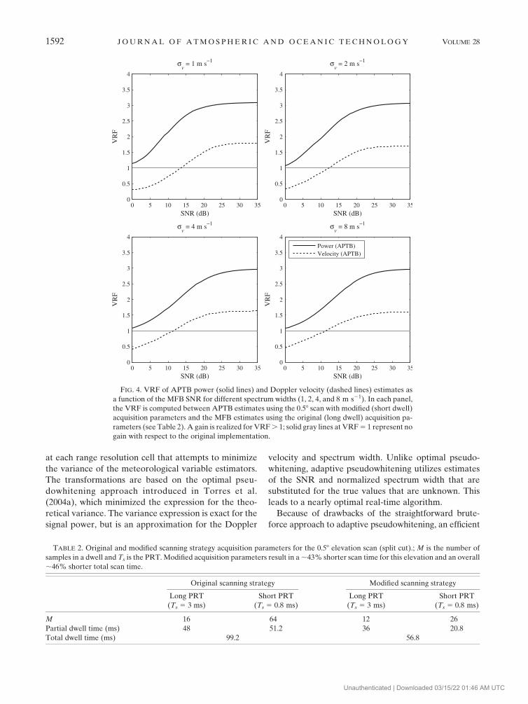
Simulations were conducted to quantitatively evalu-

ate the performance improvement that is realized when

using the modified scanning strategy in conjunction with

adaptive pseudowhitening. Figure 4 shows the variance

reduction factor of APTB power and Doppler velocity

estimates as a function of the MFB SNR for different

spectrum widths. Simulations were run for the same

acquisition parameters used in the 0.58 elevation scan of

the original and modified scanning strategies (Table 2)

and statistics were computed from 100 000 realizations.

The VRF was computed between APTB estimates with

the modified acquisition parameters and MFB estimates

with the original acquisition parameters. Although the

total number of samples was reduced by about half, the

performance of APTB power estimates using the mod-

ified scanning parameters is always better than using

original scan parameters and MFB processing in the range

of SNRs and spectrum widths depicted in Fig. 4. The trend

of the variance reduction curves toward smaller SNRs

would indicate crossover points at negative SNRs. How-

ever, this is not relevant because only significant power

data (SNR . 2 dB) are used in displays and algorithms.

On the other hand, APTB Doppler velocity estimates

using modified scan settings are only better than the

original data for SNRs above 11.3–13.5 dB, depending

on the spectrum width. For SNRs less than 11.3–13.5 dB

that are also larger than the significant-return SNR

threshold for Doppler velocity of 3.5 dB, the new pro-

cessing and acquisition parameters could result in a vari-

ance increase of up to 2 times (an ;40% increase in

standard deviation). However, the advantages of higher

temporal data resolution and by-and-large improved

data quality obtained with the modified scanning strat-

egy outweigh the performance degradation of Doppler

velocity estimates at low SNRs.

5. Conclusions

An efficient real-time implementation of adaptive pseu-

dowhitening was employed on the NWRT showing that

update times could be reduced by about a factor of 2

compared to conventional matched-filter processing with

improved data quality under most conditions. Adaptive

pseudowhitening addresses the limitations of whitening at

low SNRs by choosing a moment-specific transformation



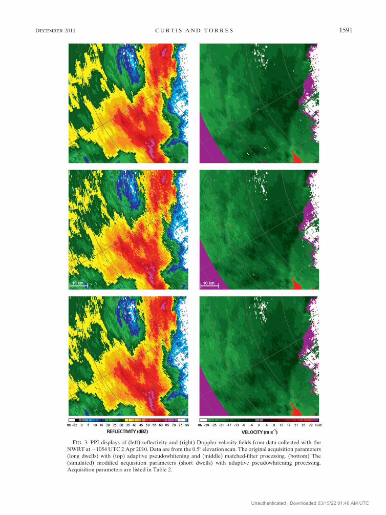
FIG. 3. PPI displays of (left) reflectivity and (right) Doppler velocity fields from data collected with the

NWRT at ;1054 UTC 2 Apr 2010. Data are from the 0.58 elevation scan. The original acquisition parameters

(long dwells) with (top) adaptive pseudowhitening and (middle) matched-filter processing. (bottom) The

(simulated) modified acquisition parameters (short dwells) with adaptive pseudowhitening processing.

Acquisition parameters are listed in Table 2.



at each range resolution cell that attempts to minimize

the variance of the meteorological variable estimators.

The transformations are based on the optimal pseu-

dowhitening approach introduced in Torres et al.

(2004a), which minimized the expression for the theo-

retical variance. The variance expression is exact for the

signal power, but is an approximation for the Doppler

velocity and spectrum width. Unlike optimal pseudo-

whitening, adaptive pseudowhitening utilizes estimates

of the SNR and normalized spectrum width that are

substituted for the true values that are unknown. This

leads to a nearly optimal real-time algorithm.

Because of drawbacks of the straightforward brute-

force approach to adaptive pseudowhitening, an efficient

TABLE 2. Original and modified scanning strategy acquisition parameters for the 0.58 elevation scan (split cut).; M is the number of

samples in a dwell and Ts is the PRT. Modified acquisition parameters result in a ;43% shorter scan time for this elevation and an overall

;46% shorter total scan time.

Original scanning strategy Modified scanning strategy

Long PRT

(Ts 5 3 ms)

Short PRT

(Ts 5 0.8 ms)

Long PRT

(Ts 5 3 ms)

Short PRT

(Ts 5 0.8 ms)

M 16 64 12 26

Partial dwell time (ms) 48 51.2 36 20.8

Total dwell time (ms) 99.2 56.8

FIG. 4. VRF of APTB power (solid lines) and Doppler velocity (dashed lines) estimates as

a function of the MFB SNR for different spectrum widths (1, 2, 4, and 8 m s21). In each panel,

the VRF is computed between APTB estimates using the 0.58 scan with modified (short dwell)

acquisition parameters and the MFB estimates using the original (long dwell) acquisition pa-

rameters (see Table 2). A gain is realized for VRF . 1; solid gray lines at VRF 5 1 represent no

gain with respect to the original implementation.



algorithm was introduced that reduces the computational

complexity by a factor of 3 (in the NWRT implementa-

tion) along with some other benefits. The main additional

benefit is the improvement to the ground clutter filtering

process. By splitting the pseudowhitening transformation

into two parts, the time series data are only filtered once.

In contrast, when using the brute-force approach, either

the time series data need to be filtered for each meteo-

rological variable or a very specific type of ground clutter

filter needs to be used to produce filtered times series

data. This greatly limits the types of filters that can be

applied. In addition to more flexibility in ground clutter

filtering, the efficient implementation also produces

digital matched-filtered time series data as a by-product

of the two-part transformation approach. Although the

efficient implementation greatly improves on the brute-

force approach, the computational requirements are still

increased by approximately the oversampling factor

compared to digital matched-filter processing. Even

though this is a significant increase in computational

complexity, the distributed computing platform utilized

for the NWRT signal processor allows for this efficient

real-time algorithm to be implemented.

To take advantage of the real-time implementation,

scanning strategies were modified to reduce scan update

times by about a factor of 2. The improvements realized

by these modified strategies were illustrated in section 4

using weather data from the NWRT. The modified scan-

ning strategy parameters were selected with the primary

goal of obtaining faster updates with overall comparable

data quality. Simulations show that these modified strat-

egies combined with adaptive pseudowhitening lead to

signal power estimates that are always better than matched-

filter processing and yield only slightly degraded perfor-

mance for Doppler velocity estimates at low SNRs. If the

velocity estimates need to be improved in this SNR range,

longer update times could be traded for further variance

reduction. For example, the dwell times of the modified

scanning strategy could be increased until the variance of

velocity estimates using adaptive pseudowhitening pro-

cessing equals that of the matched filter with the original

scanning strategy parameters at the usual SNR threshold

of 3.5 dB. Nevertheless, in most cases, the advantages of

higher temporal resolution and better performance at

medium and high SNRs should outweigh the decreased

performance at low SNR values.

In the future, this technique could be applied to other

radar systems, both those using phased-array antennas

and those using reflector antennas (e.g., the WSR-88D).

Additionally, this work should be able to be easily ex-

tended to the estimation of dual-polarization variables

(Torres and Zrnic 2003b; Torres and Ivic 2005). Through

signal processing, adaptive pseudowhitening adds a new

dimension to the traditional trade-off triangle, which in-

cludes variance of estimates, spatial coverage, and update

times. By increasing the computational complexity, it is

possible to both decrease the update times and improve

the variance of estimates without affecting the spatial

coverage.

Acknowledgments. The authors thank the anonymous

reviewers, Dick Doviak, and Igor Ivic for providing

comments to improve the manuscript and also the team

of engineers and software developers at NSSL that made

the real-time implementation of this technique on the

NWRT possible. Funding was provided by NOAA/

Office of Oceanic and Atmospheric Research under

NOAA-University of Oklahoma Cooperative Agreement

NA17RJ1227, U.S. Department of Commerce.

APPENDIX A

Equivalence of Brute-Force and Efficient AdaptiveRange Oversampling Implementations

Let V be the L 3 M complex-valued matrix of over-

sampled time series data, where L is the oversampling

factor and M is the number of samples along the sample

time. This matrix can be written as V 5 (V0, V1, . . . ,

VM21), where the Vm are L 3 1 column vectors of range-

oversampled signals at sample time m. Transformed

oversampled signals are obtained as X 5 WV, where W is

the transformation matrix and X is the transformed time

series matrix with the same structure as V. A partial

transformation of V is defined as ~X 5 P*TV, where P is

a unitary matrix from the decomposition of W as W 5

gS1P*T, where g is the transformation gain and S1 is

a diagonal real-valued matrix.

To see the equivalence between the two-step efficient

implementation and the brute-force approach, the auto-

covariances calculated from the transformed matrix X

can be shown to be identical to appropriately weighting

the L autocovariances computed from the rows of the

partially transformed matrix ~X. As described in steps 4

and 5 of the brute-force approach given in section 3, the

lag-k autocovariance estimate is obtained as the average

of the L range-oversampled autocovariances computed

from the rows of X; that is,

RX(k) 51

L�L21

l50R

(l)

X (k)

51

L�L21

l50

1

M 2 jkj �M2jkj21

m50X*(l, m)X(l, m 1 k)

24

35.

(A1)



This equation can be written in vector form by switching

the summation order, combining the constants, and

expressing the length L columns of X as Xm

5 WVm

,

where m represents sample time as

RX(k) 51

(M 2 jkj)L�

M2jkj21

m50�L21

l50X*(l, m)X(l, m 1 k)

51

(M 2 jkj)L�

M2jkj21

m50Xm*

TXm1k. (A2)

Substituting the expressions for Xm given previously and

the expression for W from (5), the summation can be

rewritten as a weighted dot product,

RX(k) 51

(M 2 jkj)L�

M2jkj21

m50(Vm*

TgPS1)(S1P*TgVm1k)

51

(M2 jkj) �M2jkj21

m50(P*TVm)*T

(gS1)2

L(P*TVm1k).

(A3)

The vectors in the summation are the partially trans-

formed columns of ~X, where ~Xm 5 P*TVm, and the

middle expression of the summation is a diagonal matrix

D 5 gL15 (gS1)2/L, which weights the dot product,

where g 5 g2/L and L1 5 (S1)2. This alternate formu-

lation of the diagonal weighting matrix D in terms of

eigenvalues instead of singular values simplifies the

steps of the efficient implementation. With these defi-

nitions the previous equation becomes

RX(k) 51

(M 2 jkj) �M2jkj21

m50Xm*

TD ~Xm1k. (A4)

The final step is to replace the weighting from the di-

agonal matrix D with an additional summation using

a new length L weight vector d 5 (d0, d1, . . . , dL21),

where dl 5 gl1l , and l1

l is the lth element of the diagonal

matrix L1. This notation for the l1l was chosen because

just as S1 is based on the singular values of H; the di-

agonal matrix L1, and thus the l1l , are based on the ei-

genvalues of CV . After replacing the diagonal weighting

matrix D with the new weight vector d, the autocovar-

iance of X can be written as a double summation similar

to the first step in (A2),

RX(k) 51

M 2 jkj �M2jkj21

m50�L21

l50dl

~X*(l, m) ~X(l, m 1 k).

(A5)

Because d does not depend on M, the double summation

can be rearranged as

RX(k) 5 �L21

l50dl

1

M 2 jkj �M2jkj21

m50

~X*(l, m) ~X(l, m 1 k)

24

35.

(A6)

The final step shows that the autocovariance from X can

be expressed as a weighted sum of L range-oversampled

autocovariance estimates R(l)~X (k), computed from ~X as

RX(k) 5 �L21

l50dlR

(l)~X (k). (A7)

This provides flexibility in computing moment-specific

autocovariances by using appropriate choices for the

weight vector d.

APPENDIX B

Computational Complexity of Adaptive RangeOversampling

In this appendix, the computational complexity of adap-

tive range oversampling using the efficient implementation

is compared to that of the brute-force implementation and

digital matched-filter processing. The following algorithm

analyses are not tied to any specific signal processing ar-

chitecture or clock rate; only the computationally expen-

sive steps are considered to approximately measure the

relative complexity of the different implementations.

Assume that a total of E meteorological variable es-

timates are computed from an L 3 M matrix of range-

oversampled data, where M is the number of samples

along sample time and L is the oversampling factor. For

example, E 5 3 for a typical single-polarization radar

(i.e., required variables are signal power, Doppler ve-

locity, and spectrum width), and E 5 6 for a dual-

polarization radar using the simultaneous transmission

and reception mode (i.e., required variables are those

for a single-polarization radar plus differential reflec-

tivity, differential phase, and magnitude of the cross-

correlation coefficient). The number of meteorological

variables may vary from the typical values depending on

the radar mode (e.g., E 5 1 for the surveillance mode,

whereby only signal power is needed) or depending on

specific processing functions [e.g., E . 3 when employing

multiple spectrum-width estimators as part of the hybrid

spectrum-width estimator developed by Meymaris et al.

(2009)]. In general, each of these meteorological vari-

ables is computed as a function of one or more



covariance estimates (e.g., the Doppler velocity is

a function of the lag-1 autocovariance estimate, and the

spectrum width is a function of both lag-0 and lag-1 au-

tocovariance estimates). Let Ctotal be the total number of

covariance estimates and Clags be the total number of

unique covariance lags needed to compute the E mete-

orological variables For example, for the NWRT PAR

implementation Ctotal 5 4 (i.e., lag 0 for signal power, lag

1 for Doppler velocity, and lags 0 and 1 for spectrum

width) and Clags 5 2 (i.e., lags 0 and 1 for the three

spectral moments). For a more general result, the com-

putational complexity of the different implementations

will be expressed as a function of L, M, E, Ctotal, and Clags.

In the brute-force implementation described in sec-

tion 3, the computationally expensive steps are (a) digital

matched filtering (step 1), (b) oversampled data trans-

formations (step 3), (c) ground clutter filtering, and (d)

oversampled covariance computations (step 4). Note that

because the meteorological variable estimation process is

common to all implementations, it is excluded from the

analysis. The digital matched filter in Eq. (1) requires

(L 2 1)M complex additions and LM complex multi-

plications. Each of the required E oversampled data

transformations [see Eq. (2)] requires L(L 2 1)M com-

plex additions and L2M complex multiplications. Ground

clutter filtering is common to all implementations (but

with varying degrees of computational complexity) and

will be addressed later. Finally, each of the L oversampled

covariance estimates requires M 2 k 2 1 complex addi-

tions and M 2 k complex multiplications, where k is the

covariance lag. Because M � k, these numbers can be

approximated by M. For the implementation on the

NWRT PAR, two autocovariance estimates at lag-0 (k 5

0) and two at lag-1 (k 5 1) are needed. The total number

of complex additions and complex multiplications ex-

cluding ground clutter filtering are listed in Table B1.

In the efficient implementation, computationally ex-

pensive steps are (a) oversampled data transformation

(step 1), (b) ground clutter filtering, and (c) autocovar-

iance estimations (step 2). Basic operations in steps a, b,

and c of the efficient implementation require the same

number of computations as steps b, c, and d of the

brute-force implementation, respectively. However, in

the efficient implementation the operations in steps

a and b are done only once and the operations in step c

are done once for each unique autocovariance lag. For

the implementation on the NWRT PAR, lag-0 (k 5 0)

and lag-1 (k 5 1) autocovariance estimates are needed.

Complex additions and complex multiplications are to-

taled in Table B1.

The computationally expensive steps of conventional

digital matched-filter processing are (a) digital matched

filtering, (b) ground clutter filtering, and (c) autocovar-

iance estimations. Basic operations in steps a, b, and c

require the same number of computations as steps a, c,

and d of the brute-force implementation, respectively.

However, for digital matched-filter processing the op-

erations in step b are done only once and the operations

in step c are done once for each unique autocovariance

lag. The total number of complex additions and complex

multiplications for digital matched-filter processing are

also listed in Table B1 as a reference.

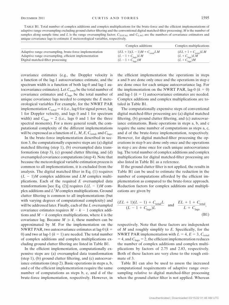
If the ground clutter filter is not applied, the results in

Table B1 can be used to estimate the reduction in the

number of computations afforded by the efficient im-

plementation as compared to the brute-force approach.

Reduction factors for complex additions and multipli-

cations are given by

(EL 1 1)(L 2 1) 1 CtotalL

(L 2 1 1 Clags)Land

EL 1 1 1 Ctotal

L 1 Clags

,

(B1)

respectively. Note that these factors are independent

of M and roughly simplify to E. Specifically, for the

NWRT PAR implementation with L 5 4, E 5 3, Ctotal

5 4, and Clags 5 2, the efficient implementation reduces

the number of complex additions and complex multi-

plications by factors of 2.75 and 2.83, respectively.

Both of these factors are very close to the rough esti-

mate of 3.

Table B1 can also be used to assess the increased

computational requirements of adaptive range over-

sampling relative to digital matched-filter processing

when the ground clutter filter is not applied. Whereas

TABLE B1. Total number of complex additions and complex multiplications for the brute-force and the efficient implementations of

adaptive range oversampling excluding ground clutter filtering and the conventional digital matched-filter processing; M is the number of

samples along sample time and L is the range oversampling factor; CTOTAL and CLAG are the numbers of covariance estimators and

unique covariance lags to estimate E meteorological variables, respectively.

Complex additions Complex multiplications

Adaptive range oversampling, brute-force implementation (EL 1 1)(L 2 1)M 1 CtotalLM (EL 1 1 1 Ctotal)LM

Adaptive range oversampling, efficient implementation (L 2 1 1 Clags)LM (L 1 Clags)LM

Digital matched-filter processing (L 2 1 1 Clags

)M (L 1 Clags

)M



the brute-force implementation of adaptive range over-

sampling requires EL times more complex operations

than digital matched-filter processing (12 times more for

the NWRT implementation), the efficient implementa-

tion only requires an L-fold increase (4 times more for the

NWRT implementation).

The computational complexity of the ground clutter

filter depends on the specific technique; but it can be

argued that it outweighs that of the transformation and

estimation steps described above. In fact, the mere esti-

mation of the Doppler spectrum using the periodogram

estimator has a computational complexity of O(M logM)

(in big-O notation), and this must be done once for digital

matched-filter processing but L times for each trans-

formed oversampled set for either implementation of

adaptive range oversampling. Thus, without including any

of the additional filtering operations, the number of com-

plex operations for ground clutter filtering dominates

compared to the other steps. Hence, it can be used solely

as a measure of the computational complexity for the dif-

ferent implementations. Because a spectral ground clutter

filterB1 has to be applied to E sets of transformed over-

sampled data in the brute-force implementation, it takes

E times more complex operations to filter the ground

clutter with the brute-force implementation than with the

efficient implementation where the filter is applied to one

set of transformed oversampled data, and EL times more

compared to digital matched-filter processing where the

filter is applied just once.

In summary, whether the ground clutter filter is applied

or not, the efficient implementation increases the com-

putations by a factor of L compared to digital matched-

filter processing, but reduces the number of computations

by roughly a factor of E compared to the brute-force

approach.

REFERENCES

Bluestein, H. B., and R. M. Wakimoto, 2003: Mobile radar obser-

vations of severe convective storms. Radar and Atmospheric

Science: A Collection of Essays in Honor of David Atlas,

Meteor. Monogr., No. 52, Amer. Meteor. Soc., 105–138.

——, M. M. French, I. PopStefanija, R. T. Bluth, and J. B. Knorr,

2010: A mobile, phased-array Doppler radar for the study of

severe convective storms: The MWR-05XP. Bull. Amer. Me-

teor. Soc., 91, 579–600.

Brown, R. A., V. T. Wood, and D. Sirmans, 2000: Improved WSR-

88D scanning strategies for convective storms. Wea. Fore-

casting, 15, 208–220.

Carbone, R. E., M. J. Carpenter, and C. D. Burghart, 1985: Doppler

radar sampling limitations in convective storms. J. Atmos.

Oceanic Technol., 2, 357–361.

Chiuppesi, F., G. Galati, and P. Lombardi, 1980: Optimisation of

rejection filters. IEE Proc. F Commun. Radar Signal Process.,

127 (5), 354–360.

Choudhury, S., and V. Chandrasekar, 2007: Wideband reception

and processing for dual-polarization radars with dual trans-

mitters. J. Atmos. Oceanic Technol., 24, 95–101.

Doviak, R. J., and D. S. Zrnic, 1993: Doppler Radar and Weather

Observations. 2nd ed. Academic Press, 562 pp.

Hefner, E., and V. Chandrasekar, 2008: Whitening dual-polarized

weather radar signals with a Hermitian transformation. IEEE

Trans. Geosci. Remote Sens., 46, 2357–2364.

Heinselman, P., and S. Torres, 2011: High-temporal resolution

capabilities of the National Weather Radar Testbed phased-

array radar. J. Appl. Meteor. Climatol., 50, 579–593.

——, D. L. Priegnitz, K. L. Manross, T. M. Smith, and R. W.

Adams, 2008: Rapid sampling of severe storms by the National

Weather Radar Testbed Phased Array Radar. Wea. Fore-

casting, 23, 808–824.

Ivic, I., A. Zahrai, and D. Zrnic, 2003a: Digital IF receiver—

Capabilities, tests, and evaluation. Preprints, 31th Conf. on

Radar Meteorology, Seattle, WA, Amer. Meteor. Soc., 9B.3.

[Available online at http://ams.confex.com/ams/pdfpapers/

64211.pdf.]

——, D. Zrnic, and S. Torres, 2003b: Whitening in range to improve

weather radar spectral moment estimates. Part II: Experimen-

tal evaluation. J. Atmos. Oceanic Technol., 20, 1449–1459.

Kumjian, M. R., A. V. Ryzhkov, V. M. Melnikov, and T. J. Schuur,

2010: Rapid-scan super-resolution observations of a cyclic

supercell with a dual-polarization WSR-88D. Mon. Wea. Rev.,

138, 3762–3786.

Lin, Y. J., T. C. Wang, and J. H. Lin, 1986: Pressure and temperature

perturbations within a squall-line thunderstorm derived from

SESAME dual-Doppler data. J. Atmos. Sci., 43, 2302–2327.

McLaughlin, D., and Coauthors, 2009: Short-wavelength technol-

ogy and the potential for distributed networks of small radar

systems. Bull. Amer. Meteor. Soc., 90, 1797–1817.

Meymaris, G., J. Williams, and J. Hubbert, 2009: Performance of a

proposed hybrid spectrum width estimator for the NEXRAD

ORDA. Preprints, 25th Conf. on Interactive Information and

Processing Systems (IIPS) for Meteorology, Oceanography,

and Hydrology, Phoenix, AZ, Amer. Meteor. Soc., 11B.1.

[Available online at http://ams.confex.com/ams/pdfpapers/

145958.pdf.]

Miller, L. J., and R. A. Kropfli, 1980: Part II: Experimental design

and processes. Bull. Amer. Meteor. Soc., 61, 1173–1177.

National Academies Press, 2008: Evaluation of the Multifunction

Phased Array Radar Planning Process. National Research

Council, 92 pp.

NOAA, 2006: Doppler radar meteorological observations. Part C:

WSR-88D products and algorithms. Office of the Federal Co-

ordinator for Meteorological Services and Supporting Research,

Federal Meteorological Handbook 11, FCH-H11C-2006, 23 pp.

Qiu, C.-J., and Q. Xu, 1996: Least squares retrieval of microburst

winds from single-Doppler radar data. Mon. Wea. Rev., 124,

1132–1144.

Siggia, A., and J. Passarelli, 2004: Gaussian model adaptive pro-

cessing (GMAP) for improved ground clutter cancellation and

moment calculation. Proc. Third European Conf. on Radar in

Meteorology and Hydrology, Visby, Gotland, Sweden, ERAD,

67–73.

B1 Spectral ground clutter filters are common on modern oper-

ational radars. For example, the WSR-88D uses the GMAP filter

(Siggia and Passarelli 2004), whereas the NWRT PAR uses the

CLEAN-AP algorithm (Warde and Torres 2010).



Torres, S., 2001: Estimation of Doppler and polarimetric variables

for weather radars. Ph.D. dissertation, University of Oklahoma,

158 pp.

——, and D. Zrnic, 2003a: Whitening in range to improve weather

radar spectral moment estimates. Part I: Formulation and

simulation. J. Atmos. Oceanic Technol., 20, 1433–1448.

——, and ——, 2003b: Whitening of signals in range to improve

estimates of polarimetric variables. J. Atmos. Oceanic Tech-

nol., 20, 1776–1789.

——, and I. Ivic, 2005: Demonstration of range oversampling

techniques on the WSR-88D. Preprints, 32nd Int. Conf. on

Radar Meteorology, Albuquerque, NM, Amer. Meteor. Soc.,

4R.5. [Available online at http://ams.confex.com/ams/pdfpapers/

96151.pdf.]

——, C. Curtis, and J. R. Cruz, 2004a: Pseudowhitening of weather

radar signals to improve spectral moment and polarimetric

variable estimates at low signal-to-noise. IEEE Trans. Geosci.

Remote Sens., 42, 941–949.

——, Y. Dubel, and D. Zrnic, 2004b: Design, implementation, and

demonstration of a staggered PRT algorithm for the WSR-

88D. J. Atmos. Oceanic Technol., 21, 1389–1399.

——, C. Curtis, I. Ivic, D. Warde, E. Forren, J. Thompson,

D. Priegnitz, and R. Adams, 2010: Update on signal processing

upgrades for the National Weather Radar Testbed. Preprints,

26th Int. Conf. on Interactive Information and Processing

Systems (IIPS) for Meteorology, Oceanography, and Hydrol-

ogy, Atlanta, GA, Amer. Meteor. Soc., 14B.2. [Available

online at http://ams.confex.com/ams/pdfpapers/163745.pdf.]

Warde, D., and S. Torres, 2010: Automated real-time mitigation of

ground clutter contamination for Doppler weather radars.

Preprints, Sixth European Conf. on Radar Meteorology and

Hydrology (ERAD), Sibiu, Romania, Romanian National Me-

teorological Administration, P2.10. [Available online at http://

www.erad2010.org/pdf/POSTER/02_Advances/10_ERAD2010_

0349_s.pdf.]

Weber, M. E., J. Y. N. Cho, J. S. Herd, J. M. Flavin, W. E. Benner,

and G. S. Torok, 2007: The next-generation multimission U.S.

surveillance radar network. Bull. Amer. Meteor. Soc., 88,

1739–1751.

Wilson, J. W., R. D. Roberts, C. Kessinger, and J. McCarthy, 1984:

Microburst wind structure and evaluation of Doppler radar for

airport wind shear detection. J. Climate Appl. Meteor., 23,

898–915.

Wurman, J., 2002: The multiple-vortex structure of a tornado. Wea.

Forecasting, 17, 473–505.

Yu, T.-Y., M. B. Orescanin, C. D. Curtis, D. S. Zrnic, and D. E.

Forsyth, 2007: Beam multiplexing using the phased-array

weather radar. J. Atmos. Oceanic Technol., 24, 616–626.

Yussouf, N., and D. J. Stensrud, 2010: Impact of phased-array radar

observations over a short assimilation period: Observing sys-

tem simulation experiments using an ensemble Kalman filter.

Mon. Wea. Rev., 138, 517–538.

Zrnic, D. S., 1975: Simulation of weatherlike Doppler spectra and

signals. J. Appl. Meteor., 14, 619–620.

——, and Coauthors, 2007: Agile beam phased array radar for

weather observations. Bull. Amer. Meteor. Soc., 88, 1753–1766.



Documents

Adaptive Range Oversampling to Achieve Faster Scanning on