Adaptive Learning For Mobile Network Management … Learning For Mobile Network Management ... Adaptive Learning For Mobile Network Management ... BTS Base Transceiver Station

Aalto University

School of Science

Degree Programme in Computer, Communication, and Information Science

Binda Pandey

Adaptive Learning For Mobile NetworkManagement

Master’s ThesisEspoo, November 2, 2016

Supervisor: Docent Tomi Janhunen, Aalto UniversityAdvisor: Jussi Rintanen D.Sc. (Tech.)

Aalto UniversitySchool of ScienceDegree Programme in Computer, Communication, and Infor-mation Science

ABSTRACT OFMASTER’S THESIS

Author: Binda Pandey

Title:Adaptive Learning For Mobile Network Management

Date: November 2, 2016 Pages: vii + 54

Major: Computer Science Code: SCI3042

Supervisor: Docent Tomi Janhunen

Advisor: Jussi Rintanen D.Sc. (Tech.)

There is an increasing demand for better mobile and network services in current4G and upcoming 5G networks. As a result, mobile network operators are findingdifficulties to meet the challenging requirements and are compelled to explorebetter ways for enhancing the network capacity, improving the coverage, as wellas lowering their expenditures. 5G networks can have a very high number of basestations, and it costs time and money to configure all of them optimally by humanoperators. Therefore, the current network operations management practice willnot be able to handle the network in the future. Hence, there will be a need forautomation in order to make the network adaptive to the changing environment.

In this thesis, we present a method based on Reinforcement Learning for au-tomating parts of the management of mobile networks. We define a learningalgorithm, based on Q-learning, that controls the parameters of base stationsaccording to the changing environment and maximizes the quality of service formobile devices. The learning algorithm chooses the best policy for providing op-timal coverage and capacity in the network. We discuss different methods fortaking actions, scoring them, and abstracting the networks’ state.

The learning algorithm is tested against a simulated LTE network and the resultsare compared against a base-line model, which is a fixed-TXP model with nocontrol. We do the experiments based on above-mentioned strategies and comparethem in order to evaluate their impact on learning.

Keywords: Mobile Networks, Reinforcement Learning, Q-learning, Net-work Management, Artificial Intelligence, Intelligent Control

Language: English

ii

Acknowledgements

I would like to express my deep gratitude to my supervisor Docent TomiJanhunen and my advisor Dr. Jussi Rintanen for giving me this opportunityto work in a challenging yet an interesting project that I present here inmy thesis. I would like to thank Tomi for his moral support, guidance andproviding the proper environment that helps me in writing this thesis in time.

I also would like to thank Jussi for his immense help and support. Hehas helped me greatly with the implementation part of this project by pro-viding ideas and correcting my mistakes. Moreover, I would appreciate himfor providing his valuable time in examining my thesis drafts regularly andcarefully that has helped me a lot to carry out my thesis work.

I further wish to extend my gratitude to Dr. Vilho Raisanen and JuhaNiiranen from Nokia Bell Labs for their collaboration and for defining theproblem in the mobile networks which has been the motivation for this work.Vilho has provided the concept of the simulated network and also designeda mini-simulator that has helped a lot for the early design of our algorithm.Moreover, he has given his valuable time by running all the experiments intheir simulated network and giving some feedback on them as well. I wouldalso like to thank Juha for running some simulations and providing ideas onthe working nature of the simulator.

Apart from this, I am grateful to the technical staff at the Departmentof Computer Science for their assistance and support. I also would like tothank Aalto University for providing computational resources.

Finally, I wish to thank all of my friends who have supported me in anyway during this tenure.

Espoo, November 2, 2016

Binda Pandey

iii

Abbreviations and Acronyms

1G First Generation2G Second Generation3G Third Generation3GPP 3rd Generation Partnership Project4G Fourth Generation5G Fifth GenerationANR Automatic Neighbor RelationsAI Artificial IntelligenceBTS Base Transceiver StationCAPEX Capital ExpenditureCCO Coverage and Capacity OptimizationCM Configuration ManagementCQI Channel Quality IndicatorDSM Dynamic Spectrum ManagementDSP Digital Signal ProcessingEDGE Enhanced Data Rates for GSM EvolutionFM Fault ManagementGSM Global System for Mobile CommunicationsICIC Inter-Cell Interference CoordinationIOT Internet of ThingsKPI Key Performance IndicatorLTE Long Term EvolutionM2M Machine to Machine CommunicationsMLB Mobility Load BalancingMMS Multimedia MessageMRO Mobility Robustness OptimizationNE Network ElementNGMN Next Generation Mobile NetworkNMS Network Management SystemOAM Operation and Maintenance

iv

OMC Operation and Maintenance CentreOPEX Operational ExpenditurePCI Physical Cell IDPM Performance ManagementPOMDP Partially Observable Markov Decision ProcessQoS Quality of ServiceRET Remote Electrical TiltRL Reinforcement LearningRLF Radio Link FailureSNR Signal to Noise RatioSON Self Organizing NetworkTD Temporal DifferenceTXP Transmission PowerUE User EquipmentUMTS Universal Mobile Telecommunications System

v

Contents

Abbreviations and Acronyms iv

1 Introduction 11.1 Structure of the Thesis . . . . . . . . . . . . . . . . . . . . . . 3

2 Background 42.1 Network Management . . . . . . . . . . . . . . . . . . . . . . 52.2 Network Data . . . . . . . . . . . . . . . . . . . . . . . . . . . 52.3 History of Mobile Telecommunication System . . . . . . . . . 6

2.3.1 From 1G to 3G . . . . . . . . . . . . . . . . . . . . . . 62.3.2 LTE and Self Organizing Network . . . . . . . . . . . . 7

2.4 Need for Intelligent Automation . . . . . . . . . . . . . . . . . 82.5 Related Work on Automation of Network Management . . . . 9

3 Reinforcement Learning 103.1 Introduction . . . . . . . . . . . . . . . . . . . . . . . . . . . . 103.2 Elements of Reinforcement Learning . . . . . . . . . . . . . . 123.3 Q-Learning . . . . . . . . . . . . . . . . . . . . . . . . . . . . 133.4 Types of Reinforcement Learning . . . . . . . . . . . . . . . . 143.5 Reinforcement Learning in Network Management . . . . . . . 16

4 Learning Algorithm for Adaptive Networks 184.1 The Learning Algorithm . . . . . . . . . . . . . . . . . . . . . 194.2 State Space . . . . . . . . . . . . . . . . . . . . . . . . . . . . 204.3 Abstraction of the State Space . . . . . . . . . . . . . . . . . . 21

4.3.1 Partitioning the CQI Classes into Components . . . . . 224.3.2 Abstracting Values for the Components . . . . . . . . . 23

4.4 Actions . . . . . . . . . . . . . . . . . . . . . . . . . . . . . . 264.5 Learning Rate . . . . . . . . . . . . . . . . . . . . . . . . . . . 264.6 Scoring Function for States and Abstract States . . . . . . . . 28

4.6.1 Unabstracted Score . . . . . . . . . . . . . . . . . . . . 28

vi

4.6.2 Abstracted Score . . . . . . . . . . . . . . . . . . . . . 304.7 Rewards for Actions . . . . . . . . . . . . . . . . . . . . . . . 314.8 Q-Value Updates . . . . . . . . . . . . . . . . . . . . . . . . . 32

4.8.1 Choice of γ . . . . . . . . . . . . . . . . . . . . . . . . 33

5 Experiments and Results 345.1 Setting . . . . . . . . . . . . . . . . . . . . . . . . . . . . . . . 345.2 Experiments . . . . . . . . . . . . . . . . . . . . . . . . . . . . 36

5.2.1 Base-Line Model . . . . . . . . . . . . . . . . . . . . . 365.2.2 Different Number of Abstract Values . . . . . . . . . . 365.2.3 Different Numbers of Components . . . . . . . . . . . . 405.2.4 Weight Vectors and Randomization in Choosing Actions 41

5.3 Result Analysis . . . . . . . . . . . . . . . . . . . . . . . . . . 44

6 Discussion 456.1 Factors Affecting Learning . . . . . . . . . . . . . . . . . . . . 456.2 Possible Variations and Prospects for Future Work . . . . . . 46

7 Conclusions 48

vii

Chapter 1

Introduction

In the past few years, there has been a rapid increase in the number of mobilesubscribers as well as in the use of new data services such as social networking,video streaming, and so on in mobile telecommunications networks. More-over, recent technologies, such as smartphones and tablets have powerfulprocessors and support high-end multimedia applications. In addition, theconcept of Machine to Machine (M2M) communications is emerging rapidlydue to automation and Internet of Things (IOT). These all have caused themobile data traffic to grow exponentially [16] and hence there is a high de-mand for enhancing the network capacity and improving Quality of Service(QoS).

This leads to the advent of Long Term Evolution (LTE) in the hope ofachieving the strong requirements posed by the current situation in cellularnetworks as well as getting the cost per bit down [16, 40]. LTE refers to thelatest standard for high-speed wireless data communication networks which iscapable of increasing the network capacity and speed using new digital signalprocessing techniques (DSP). However, handling the larger data volume inLTE in different cell contexts is a real challenge for network management.The number of base stations will increase and the effort of maintaining themincreases as well. Moreover, most of the network management functions suchas network planning, configuration, management, healing, and optimizationrequire substantial work effort and high cost, both on capital investment andoperational expenditures (CAPEX and OPEX) [16, 40], and handling suchfunctions manually is all the more difficult. Apart from that, manual effortis time-consuming and prone to errors. Thus, manual configuration of eachnetwork element becomes gradually impossible with the growing number ofnetwork elements. Hence, there is a need for automation of these tasks sothat the network operation expenses get minimized and Quality of Service(QoS) gets improved in terms of connection reliability, data bandwidth, and

1

CHAPTER 1. INTRODUCTION 2

latency.Recently, an emerging concept called Self Organizing Network (SON) is

being introduced to address these challenges in current 4G and upcoming 5Gnetworks. SON aims at increased automation of network operations in orderto utilize network resources in an optimized way. Currently, SON consists ofnumerous functions for automatic configuration, optimization, and healingof mobile networks [33]. These functions are implementations of use casesand implementing numerous use cases is a cumbersome job. A more pressingproblem, however, is tailoring the the behavior of existing SON functiontypes to different cell contexts and coordinating their behavior. Furthermore,global optimization of network is futile, as the situation changes continuouslyand it is hence better to perform localized optimizations to address specificissues. Therefore, the future goal is to introduce an automated networkmanagement function which can learn from data and adapt.

In this thesis, we are investigating adaptive methods for cellular networkmanagement at the level of base stations. In particular, the work attemptsto find methods for learning useful management policies for SON functionssuch as adjusting the main transmission parameters of base station antennas,primarily transmission power and antenna tilt. We adopt the framework ofreinforcement learning [38] and use the independent learning approach wherethe network parameters of base stations are adjusted independently withoutglobally optimizing the parameters of all base stations jointly. The approachignores the network parameters of other base stations. The reason behindchoosing the independent approach instead of joint learning is due to the goodscalability of independent learning. There is a large number of base stationsand optimizing each of their parameters will result in very large state spacesif the situation of other base stations is also considered when adjusting theparameters of one. On the other hand, the state space is manageable if thelearning is independent.

The state space of mobile networks has an astronomical size, but can besignificantly reduced by abstraction. Hence, one of the goals of this thesis isto design abstraction methods which accurately abstract the network state.We provide various ways of abstracting the given network state and comparethem. Our further aim is to define methods for scoring actions in terms theirimpact on QoS and examine their effects on learning. In addition, we evaluatedifferent exploration/exploitation policies in choosing the best settings in thenetwork and perform experiments based on them as well.

CHAPTER 1. INTRODUCTION 3

1.1 Structure of the Thesis

The structure of the thesis is as follows. In Chapter 2 we give an overview ofmobile networks and network parameters. Here, we focus on current prac-tices for network management. Further, we discuss the difficulties of thecurrent approaches to the management of the current 4G and upcoming 5Gnetworks and conclude the chapter by showing that there is a need for anautomated approach for the efficient management of the networks. In Chap-ter 3 we present the theory behind reinforcement learning in detail. Weexplain essential elements of reinforcement learning and its types and focuson Q-learning. In Chapter 4 we present our learning algorithm designedfor network management including abstraction methods, scoring functions,and exploration and exploitation policies. In Chapter 5 we study the perfor-mance of the methods of Chapter 4. In Chapter 6 we discuss issues relatedto our learning method and also provide possible extensions for future work.We finally give a brief summary of the whole thesis work and make someconcluding remarks.

Chapter 2

Background

A mobile network [12] is a wireless communication network which providesradio coverage to large geographical areas. A mobile network user can con-nect his or her mobile terminal, such as a mobile phone or a tablet, to thenetwork and move within the service area without losing the connection tothe network. The continuous coverage is provided by placing base transceiverstations (BTS) at various locations throughout the geographical area of thenetwork. Each base station contains one or more antennas which providecoverage to a limited area, called a cell. Figure 2.1 shows a typical layout ofbase stations covering a part of the mobile network.

There are several types of cells, based on their size and capacity. They areMacrocells, Microcells, Picocells, and Femtocells. Macrocells provide a widerange of coverage and are found in rural areas or highways. Microcells areof a size of few hundred metres and are suitable for densely populated urbanareas. Picocells are used for smaller areas such as offices or shopping centers.Finally, femtocells cover the smallest area and are installed in homes.

Figure 2.1: Typical layout of a base station

4

CHAPTER 2. BACKGROUND 5

2.1 Network Management

A mobile network is run by a network operator and the network operationsare operated through a centralized Operation, Administration, and Main-tenance (OAM) architecture. The key element of OAM is Operation andMaintenance Centre (OMC) which is responsible for monitoring the network,configuring the network parameters, and optimizing the network behavior.Network Management System (NMS) is the main part of OMC that oper-ates the network. The operator can monitor and access the network elements(NEs) by using a software system called NMS. The network management in-cludes a larger set of functions which are included in following functionalareas [17, 25].

• Fault management (FM) provides information on the status of the net-work. Any malfunctions in the network component are detected andtransferred to NMS so that technicians can repair them.

• Configuration management (CM) functions deal with network config-uration parameters such as frequency plans and handover algorithmswhich are directed from NMS to all NEs.

• Performance management (PM) is responsible for monitoring networkperformance. The data from all network elements is collected by theNMS for further processing and analysis.

• Security management is responsible for handling security measures,such as system logs and access control.

2.2 Network Data

Network elements produce PM and FM data (measurement and alarms)whereas CM data are typically created by NMS (including SON functions).NMS collects these data for further analysis. These data can be dividedinto three categories, system configuration data, system parameter data, anddynamic data [17]. System configuration data tells about the configurationand organization of the network such as BTS locations and transmissionnetwork topology. These types of data are highly persistent and are not usu-ally modified once the network is deployed. System parameter data definesthe way the system functions are implemented and operated within the net-work. Examples of such data include antenna transmitter output power and


BTS threshold for the maximum number of accepted simultaneous connec-tions. These parameters can be either modified by the network operator orby autonomous processes according to the changes in the traffic conditions.Finally, dynamic data consists of the measurement values and statistical timeseries, alarms, and other events. These data describe the dynamic use of thenetwork and its functions [17].

The system parameter data is handled by configuration managementfunctions. Parameter changes are defined in the NMS and then deployedto NEs. The events occurring in various NEs are counted and recorded dur-ing the operation of the network, thereby generating counters [25]. Timeframes like 15 minutes, one hour, or one day, are used in the counting formanagement purposes. These counter values are analyzed in order to gaininformation on the network performance. However, the number of countersis huge and it becomes a complex task and impractical to use all of them.Therefore, they are usually aggregated to higher level variables called KeyPerformance Indicators (KPI) [39]. These KPI will provide an overview ofthe cell states in the mobile network.

In this work, we concentrate on Radio Link Failure (RLF) and ChannelQuality Indicator (CQI). RLF event occurs when a terminal loses its connec-tion to the network. A terminal frequently sends a CQI report to the BTS[12]. CQI reports indicate maximum data rates that the terminals can reach.

2.3 History of Mobile Telecommunication Sys-

tem

2.3.1 From 1G to 3G

First generation systems [12] were based on analog communication techniquesintroduced in the early 1980s. The networks had very large cells and the ra-dio spectrum was not used efficiently. Thus, the capacity of the networkwas comparatively small. After a decade, these systems were replaced by2G digital telecommunications which were more efficient in the use of theradio spectrum. 2G technologies were originally designed for voice and werelater enhanced to support data services such as text messages, picture mes-sages, and multimedia messages (MMS). The most popular 2G system wasthe Global System for Mobile Communications (GSM). With the increasein the data rates over the Internet, 3G systems were introduced using tech-niques such as Enhanced Data Rates for GSM Evolution (EDGE) to fa-cilitate growth, increase bandwidth, and support more diverse applications.


The most dominant 3G system is the Universal Mobile TelecommunicationSystem (UMTS).

2.3.2 LTE and Self Organizing Network

Mobile data traffic started to increase dramatically due to the introductionof new technologies such as Apple’s iPhone and Google’s Android operatingsystem for mobile phones. These smartphones support many mobile appli-cations that require Internet with higher data rates [12]. The problem withdata growth in 3G is too high cost per bit. Hence, there was an urgent needto upgrade the network. Thus, the concept of LTE was introduced. LTE isa 4G communication standard which evolved from the 3G technology and isan enhancement of UMTS (Universal Mobile Telecommunication Systems).LTE is faster than UMTS (one of the 3G systems) and thus supports fea-tures such as a high data rate, low transmission latency, lower cost per bit,and packet optimized radio access networks [3, 16]. LTE also provides muchgreater spectral efficiency than the most advanced 3G networks.

However, the configuration of cells for large data volumes becomes prob-lematic in LTE. The configuration, planning, and optimization of networkelements are done by human operators and this becomes infeasible with theincrease in the number of base stations. Thus, the concept of Self OrganizingNetworks (SON) becomes an integrated part of LTE which aims at reducingexpenses by automating the network operations. SON has a self-organizingcapability that enables the network to configure itself, thereby reducing thecomplexity, cost, and time. SON consists of a set of functions which aredefined by the 3rd Generation Partnership Project (3GPP) and the NextGeneration Mobile Network (NGMN) alliance [24] and, can be categorizedinto three functional areas.

• Self-Configuration is the process of providing ”plug and play” function-ality in network elements which minimizes the human intervention inthe overall installation process when new components are added into anetwork. It involves several distinct functions such as automatic soft-ware management, physical cell ID configuration (PCI) and automaticneighbor relations (ANR) [33]. Self configuration should take care ofthe tasks such as bringing new NEs or NE parts, automatic connectiv-ity setup between the NE and the OAM system, as well as automaticconfiguration of BTS radio parameters.

• Self-optimization functions aim at maintaining the quality and per-formance of the network with minimum manual intervention. These


functions analyze the performance of network elements and automat-ically trigger optimal actions. Automatic neighbor relations (ANR),inter-cell interference coordination (ICIC), mobility load balancing op-timization (MLB), and mobility robustness optimization (MRO) aresome of the important self-optimization SON functions [33]. ANR isused both in self-configuration and optimization. Neighbor relationsneed to be set up during the configuration of each NE. In addition,they need to be maintained during run time because of the change incoverage areas and handover behavior.

• Self-healing functions aim at detecting malfunctions and resolve or mit-igate them, thereby reducing maintenance costs [33].

Network coverage and capacity is one of the important objectives in mo-bile networks and is also the main focus of this thesis. This objective isachieved by one of the important SON functions called Coverage and Ca-pacity Optimization (CCO) [24]. The coverage and capacity of a cell mayvary due to changes in the environment. The changes can be due to season,such as trees in full leaf during summer, heavy snowfall during winter, orman-made changes in the environment. The requirements in coverage andcapacity may also change due to variations in traffic distribution, for exam-ple in city centre during rush hour. CCO adjusts the transmission powerand antenna tilt to avoid any gaps in coverage. However, unnecessary over-lapping between cells might lead to interference. Therefore, CCO needs toadjust the transmission parameters so that the coverage is good as well asthe interference is minimized [16].

SON functions reduce human effort in managing a network. However,interference between these functions may lead to coordination problems [24,34]. For example, a conflict occurs when two instances of a CCO functionchange the parameters of two neighboring sectors simultaneously [24].

Individual SON functions perform well in separation. However, in jointoperation, the impact on the network performance is not always the best. Tomitigate such coordination problems, the dependencies among SON functionshave to be reduced. But, it becomes infeasible to fix all possible conflictsmanually as the number of SON functions increases.

2.4 Need for Intelligent Automation

As discussed above, the SON functions are capable of optimizing and main-taining the mobile network. In the existing system, human operators defineall the objectives in the form of parameters and policies for configuring the


behavior of SON functions. These parameters and policies depend on thenetwork environment and the technical properties of the network. SON usesthe rule set defined by human operators and has difficulties in adapting thechanging network on its own. New rules need to be defined to cope up withevery specific network state which is not feasible as the network grows large.In addition, optimizing the configurations for many cells having differentcharacteristics (different numbers of users, different data usage patterns) isanother problem and demands more manpower. The future networks adapt-ing 5G technology will be highly dynamic and will have frequent changesin the operational context. Therefore, SON functions need to be highly in-telligent and possibly automated so that the cells can adjust their settingson their own according to the changing environment. Thus, AI technologiesand machine learning need to be adapted to make the SON functions moreintelligent and less dependent on human operators [16].

2.5 Related Work on Automation of Network

Management

Much research has been done regarding the automation of mobile networks.In [40], an automated method was proposed to deal with self-healing func-tions. The method had two main steps: detection and diagnosis. Detectionof an anomaly was done by monitoring the performance indicators (KPI) andcomparing them to their usual behavior. In diagnosis, the reports of previousfault cases were looked up and best matching root causes were identified.

Raisanen et al. [10] have presented a demonstrator system that is capableof detecting network failures and recovering from them automatically. Theydefined two steps to solve this task : anomaly analysis and recovery analysis.In anomaly analysis, abnormal cells were detected by using user measurementreports. Data mining approach (k-nearest neighbor) was used to classify acell as normal or abnormal. In the second stage, solutions are proposed basedon an anomaly report. They used a case based reasoning algorithm to selectthe best recovery actions.

Chapter 3

Reinforcement Learning

3.1 Introduction

Reinforcement learning [38] is a form of machine learning where an agentlearns to interact with an unknown environment in order to maximize itsnumerical reward. The reward is the feedback obtained from the environ-ment whenever an action is taken. The agent learns to act and optimize itsbehavior from the feedback obtained from its actions [21]. That means, forthe first time, if an agent takes an action and receives a bad response forit from the environment, then from the next time onwards it learns not tochoose the same action in that state. For example, a child who is burned byfire will learn not to go near fire.

Figure 3.1 is a general architecture of RL that depicts agent-environmentinteraction. The agent takes an action that changes the state of the environ-ment. Subsequently, the environment gives feedback in the form of a reward.The reward can either be positive or negative. It is a continuous processwhere an agent receives a new state (st) and reward (rt) for each time step tand gradually learns to take the best action (at). The utility of the agent isdefined by the reward function, and the agent must learn to act to maximizethe expected reward.

10

CHAPTER 3. REINFORCEMENT LEARNING 11

Figure 3.1: Agent-Environment Interface in Reinforcement learning

Reinforcement learning is different from supervised learning. Supervisedlearning is learning from examples where the examples and the associatedfeedback are provided by experts. However, in reinforcement learning theagent is not trained with training examples and hence is not explicitly toldabout the difference between good and bad actions. By good actions, wemean the actions that lead to high rewards in the long run and by badactions, we mean the actions that lead to negative rewards or costs. Hence,the objective of reinforcement learning is to make the agent intelligent sothat it can discover the best actions from its own experience. In order toachieve this, the agent should learn to recognize good and bad actions bytrial and error. The next important thing about choosing actions is that, inmany cases some actions give a high immediate reward but in the long run,fail to maximize the long term reward. But, the objective of reinforcementlearning is always about choosing the actions that maximize the long termreward. Some examples of reinforcement learning are the following.

• When learning to crawl, any forward motion can be considered a posi-tive reward [36].

• In a chess game, when you checkmate the opponent, then it is a goodaction, and being checkmated by the opponent indicates something badhas happened and your chance of losing the game is high.

• The N-arm bandit problem [23] is a reinforcement learning problem.Here, the player has n arms to pull and receives initially an unknownand possibly stochastic payout. Hence, the player has to learn to choosethe arm that has the highest payouts.


The state space and actions in reinforcement learning are known whereastransition probabilities between states and the reward function are unknown.

3.2 Elements of Reinforcement Learning

There are four main components in reinforcement learning. They are a policy,a reward function, a value function and a model of the environment [38].

Policy Policy is stochastic mapping from states to actions. In RL, thelearning behavior is determined by the agent’s chosen policy. Agent observesthe state and chooses an action accordingly. Policy can be a simple functionor a lookup table in some cases or it may involve a extensive computation inothers.

Reward Function The reward function is a mapping of the state of theenvironment to a numerical value. The function should distinguish betweengood and bad events for the agent. It indicates the immediate reward foractions.

Value function Reward function gives immediate payoff for a givenstate and hence is not sufficient for decision making in the long term. Hence,value function which gives long-term payoff of a state comes into play. Astate with low reward can still have a high value because it could be followedby other states that yield high rewards.

Model This is an optional element in reinforcement learning. One canfirst learn the transition probabilities among all the states and the rewardfunction for each of the states, and this information can be used to build anexplicit model of the system. Such models can be used for planning wherethe future situations are taken into account while deciding any actions incurrent situation [38]. Methods like dynamic programming [4, 5] are used inmodel-based systems in order to learn optimal value functions and to findoptimal policies from them [31]. There are many other model-free (direct)learning techniques such as Q-learning [47] and TD(λ)-methods [38] whichlearn the state value function (or the Q-value function) directly (without theneed of any explicit model) and obtain an optimal policy.

Both model-based and model-free RL methods have their own pros andcons depending on the type of problem. Atkeson et al. [2] compared model-based and model-free learning on a simple task called pendulum swing up


and observed that model-based learning is more efficient. Similarly, Wiering[49] has used a model-based RL algorithm on traffic light control. He useda model-based technique for estimating cumulative waiting time of cars. Onthe other hand, research with model-free RL techniques has also been done.Lauer and Riedmiller [26] have proposed a model-free distributed Q-learningalgorithm in cooperative multi-agent systems to find optimal policies. Sim-ilarly, Littman [29] has provided a Q-learning method for finding optimalpolicies in mutliplayer games such as soccer. Other research on model-freeQ-learning technique includes [22, 41].

We will be using the model-free technique for mobile network managementproblem and will be focusing on Q-learning only.

3.3 Q-Learning

Q-learning [47] is a widely used model-free reinforcement learning techniquewhere the Q-value of each action a in a given state s in maintained in atable. In other words, it learns the action-value function which gives theexpected utility of taking an action in a given state and thereafter follow-ing the best policy. The convergence of Q-learning to the optimum action-values has been proved under certain assumptions [46]. The values for eachstate and action are updated every time by an update function. Hence,the learning is on-line and there is no need for an explicit transition model.The general procedure for Q-learning techniques is given as Algorithm 1.

Algorithm 1: Q-learning

1 Initialize Q(s,a) with some arbitrary value (for example, 0).2 Let the current state of an agent be s.3 while True do4 a←− Action chosen by agent at time t derived from the Q-value

table.5 Action a takes the system to a state s′ and receives a reward r.6 Update Q(s, a) according to r.7 s←− s′

The learning algorithm has to try out all possible alternatives infinitelyoften in order to converge to the optimal policy. This involves both ex-ploration and exploitation [38]. However, maintaining the balance betweenexploration and exploitation is a challenging task in reinforcement learning.Exploitation means taking an action that seems best according to the already


acquired information, whereas exploration means trying out new things inthe hope of finding better actions. In order to maximize the reward, theagent has to exploit and choose the best action it knows so far. However,this does not guarantee the optimality of the solution in the long run becausethe chosen actions may not be the best ones, and there can be other unex-plored actions which can give better long-term reward [44, 45]. Therefore,exploration is important where the agent takes a risk to try out new thingswith the objective of learning. There is always a general conflict betweenlearning and obtaining high rewards. For this reason, initially there is a lowweight on obtaining high rewards, and this weight is increased later when thebest actions are known better. That means, in general, one should learn fora while by exploring different actions, and after certain stage one can exploitthe information that was learned.

There are many approaches defined to balance between exploitation andexploration. One straightforward and successful approach is ε-greedy [47].In this method, the parameter ε determines the randomness in action selec-tions and controls the amount of exploration [45]. Usually the range of ε isbetween 0 and 1. The agent chooses the best action with probability 1- ε,and otherwise, it chooses the actions at random. There are other explorationmethods that use counters [43], confidence bounds [19, 20], model learning[9], soft-max policies [31]. Among them, ε-greedy approach is a widely usedmethod and one of the reasons behind it is because memorization of explo-ration specific data is not required [44, 45]. However, choosing a good valuefor ε can be a challenging task [45].

More information regarding exploration and exploitation schemes can befound in [42].

3.4 Types of Reinforcement Learning

Two types of reinforcement learning can be distinguished based on the num-ber of agents single-agent learning and multi-agent learning [31]. Single-agentlearning is a very simple form of learning where there is a presence of onlyone agent and the environment remains stationary. The agent optimizes itsbehavior by choosing actions that maximize the reward. The idea behindmulti-agent learning is the same as single-agent except that there are severalagents interacting with the environment as well as communicating with eachother.

Learning in the multi-agent framework is more difficult than the single-agent environment. Unlike in single-agent learning, the reward in multi-agentlearning is based on the combined actions of agents. So, choosing the best


joint action for obtaining the best reward is difficult and it takes a long timefor learning to converge.

Consider an example from [11] shown in Table 3.1. There are two agentsand each of them has a choice of two actions. Agent 1 has actions a0 anda1 and Agent 2 has actions b0 and b1. The reward depends on the decisionsmade by both agents. The best rewards are obtained when agent 1 takesaction a1 and agent 2 takes action b1. But, during learning phase, agent 1 isuncertain about choosing action a1 because it could get better reward witha0, if agent 2 takes action b0 instead of b1. Hence, learning in the multi-agentframework is difficult as each agent, very often, ignores the decision of otheragents. A strong coordination among the agents need to be built to get thebest rewards.

a0 a1b0 5 0b1 0 10

Table 3.1: A two-player game. Actions a0 and a1 belong to Agent 1 and actionsb0 and b1 belong to Agent 2.

There are two forms of multi-agent learning based on how the agent in-teracts. They are independent (centralized) learning and joint (distributed)learning [11, 48].

Independent Learning Agents in independent learning are unawareof the existence of other agents or they ignore the impact of the other agents’behavior on their rewards [11]. Thus, learning for each agent is same assingle-agent learning. Each agent chooses its own actions and optimizes itsbehavior based on the rewards obtained from those actions.

Joint Learning Unlike in independent learning, each agent in jointlearning cares about the presence of other agents and shares informationamong each other, and receives a joint reward from joint actions. In otherwords, the focus of agents is on maximizing joint reward instead of maximiz-ing their individual reward.

Tan [41] suggested three different ways of agent cooperation in multi-agent RL and presented case studies for each of these approaches. In thefirst approach, agents can communicate with each other by sharing immediateinformation such as sensation and rewards. In the second, agents share the


past experiences (that others may not have experienced yet) in the form ofepisodes which is the triples consisting of sequence of a state, an action, anda reward. In the third, agents share learned policies. The results show thatcooperative learning is faster and the convergence is quicker compared toindependent learning. However, state spaces in cooperative learning are verylarge and the communication costs are high. Therefore, there is a trade-offbetween the performance and cost when cooperative learning is used.

Weiss [48] studied coordination among agents in multi-agent learning andproposed learning algorithms that make the agents act concurrently. Hestudied reinforcement learning in a setting where only one agent gets toperform and action, and all agents have to compete to get the right to bethat agent.

Wiering [49] proposed a multi-agent model-based RL method for a trafficlight control to optimize the driving policies of cars. He considered threedifferent RL designs for using current information about the state of othertraffic lights. In the first one, only local information is used to compute wait-ing time of each car. The second one used global information for computingwaiting times for the first car in the queue and local information for othercars. The third one used global information for all cars. The RL designswere compared against non-adaptable traffic light controller and the resultsshowed that the RL designs perform better. Furthermore, the performanceof each design depends on the number of cars added at each time step.

Lauer and Riedmiller [26] used a model in which multiple agents learn apolicy independently of other agents, all trying to maximize a shared rewardfunction. This work has the interesting aspect that, similarly to the cellularnetwork management problem, the agents’ goal is to maximize the overalljoint reward at the cost of their own private reward (which are a componentof the joint reward).

3.5 Reinforcement Learning in Network Man-

agement

Reinforcement learning and related techniques have earlier been used in themanagement of mobile networks. Razavi et al. [35] combined reinforcementlearning with fuzzy logic to control antenna tilt in LTE networks. The controlof a base station antenna is represented as rules with a fuzzy condition.The state space is abstracted according to qualitative parameter values, andreinforcement learning associates the best possible action with each rule. Inthis work, a global (rather than a distributed/decentralized) policy is learned,


and the feasibility of the approach is demonstrated with a model that has 7base stations with 3 antennas for each.

Bennis et al. [7] applied decentralized RL to channel selection and powercontrol of networks of micro, femto, and pico cells. The algorithm jointlyestimates the long-term utilities of femtocells and optimizes their strategies.

Bennis and Niyato [6] proposed a distributed Q-learning algorithm formanaging interference between macrocells and femtocells as well as amongneighboring femtocells. The algorithm was effective in self-organization offemtocells where each femtocell learns from the local environment and wasable to make decisions on their own. Moreover, the learning algorithm wasable to reduce interference towards the macrocell as well as manage interfer-ence among the femtocells.

Bernardo et al. [8] studied the feasibility of RL-based framework for Dy-namic Spectrum Management (DSM). The proposed framework was success-ful in performing spectrum assignment per cell dynamically in radio accessnetworks. In addition, RL algorithm stands out the best to balance betweenspectral efficiency and QoS compared to other strategies of spectrum assign-ment.

Lee et al. [27] proposed a Q-learning based approach for autonomic re-configuration of wireless mesh networks with the objective of improving thenetwork performance. Each network node in the system was able to learn agood policy in the changing environment and improve the quality of packetdelivery ratio.

Other research on network management using RL can be found in [15,28, 32].

Chapter 4

Learning Algorithm for AdaptiveNetworks

The mobile network management problem, deciding about the configurationof antenna parameters such as transmission power and antenna tilt, can beviewed as a reinforcement learning problem in which the quality-of-service ofmobile devices, in the range of the base station, is viewed as the reinforcementsignal. There are many configuration parameters, and in this work we havechosen parameters relevant to CCO SON use case. The main reason behindusing the RL approach is that, in this problem, we do not know the rewardassociated with each action in advance and hence cannot decide immediatelythe best settings for each cell. Additionally, the situation in the networkis dynamic and one-time optimization of the system is not possible evenin principle, rather one needs to optimize continuously as situation evolves.Therefore, we need to try out various possibilities of changing the networkparameters. The decisions on choosing the best action are gradually improvedby utilizing the feedback obtained from earlier decisions. The feedback in thenetwork management can be the QoS measured in terms of better connectionquality, for example. However, this application —network management—has several features that differ from the most commonly used reinforcementlearning methods.

Distributed RL The size of joint state space is NM where N is the numberof states per base station and M is the number of base stations. Due tothis large state space, the use of policies that map the joint state spaceof all base stations to a control action is infeasible. Distributed andmulti-agent variants of reinforcement learning [48] seem a better matchfor the network management application rather than doing single-agentRL with the whole network.

18

CHAPTER 4. LEARNING ALGORITHM FORADAPTIVE NETWORKS 19

State-space structure The state space with respect to the effects of pos-sible control actions is simple: for the current state of the system (i.e.,the mobile terminals and their usage status with respect to each basestation), the antenna configuration (i.e., transmission power and tilt)can be changed from any control state to any other in one step. Thusone of the main difficulties in reinforcement learning in general, thepotentially very long action sequences needed to get from one state toanother, leading to slow learning of optimal policies, is not present inthis application.

Reward function vs. observations The reward function coincides withthe observation function. The management objective is to maximizethe QoS measures, and the QoS measures are what is observed whenmaking management decisions.

We consider a basic Q-learning style algorithm adapted to the specificfeatures of the network management problem.

4.1 The Learning Algorithm

The learning algorithm for adjusting the network parameters consists of statespace, abstraction function, scoring function and exploration/exploitationpolicy. Each of these is explained thoroughly in this chapter.

We have a high number of base stations and the learning algorithm opti-mizes the network parameters of each of these independently. Each antennaof a base station, corresponding to a cell, has its own parameters to adjust,and we control the Transmission Power (TXP) of each antenna so that themeasure for overall connection quality improves. However, too high TXPcauses interference between base stations, and too low TXP weakens connec-tion to mobile terminals. Therefore, the algorithm has to find an optimalsolution to balance between the interference and connection quality. Thealgorithm starts from some initial TXP settings which are defined by thenetwork operator. The network generates a state vector called CQI, thatsummarizes the connection quality of the mobile terminals in the range ofthe base stations. This vector is already a rough abstraction of the reality ofthe network. However, identifying these vectors with the states for our learn-ing algorithm will result in a very large state space. Therefore, we apply anabstraction method which maps the values in the CQI vector to fewer values.The final state for each cell is then given by the current TXP setting andan abstracted CQI vector. The algorithm then explores a new action withsome randomization, or in other words, it changes the TXP values for each


cell and waits for the results from the network based on the changes. A newstate is reached due to the effect of the chosen setting. We then compute ascore for this new state from the CQI vector. Finally, the Q-value table forcurrent state-action pair is updated using the score of the new state. Theprocess continues and repeats the same procedure indefinitely. In the sim-ulated environment, the process can be stopped after a certain number ofiterations. However, one needs to run the algorithm for many iterations sothat the learning converges.

Algorithm 2 presents the multi-agent and independent learning algorithm,with subprocedures being explained later in more detail.

Algorithm 2: Learning Algorithm

1 counter = 12 while True do3 for cell do4 s = getstate(cell)5 %Explore action (TXP changes)%6 if randomnumber < explorationrate(counter) then7 action[cell] = arg maxa∈actionsQ

cell[s, a]8 else9 action[cell] = randomly chosen action.

10 %The network continues to run with new TXP settingsand produces new CQI vectors%

11 for cell do12 s′ = getstate(cell)13 reward = score(s′.CQI)14 Qcell[s, action[cell]] = γ×Qcell[s, action[cell]] + (1−γ)× reward15 counter = counter + 1

4.2 State Space

The current TXP value and connection quality of the terminals (based onthe TXP and the physical state of the surroundings of the base station) arethe relevant features of the network that define its state. The CQI vector,which is obtained frequently from network, gives the quality measure forall the terminals. Hence, we initially define the unabstracted states of thesystem which is composed of the TXP value and the CQI vector and laterabstract these states. We term these TXP values as the control state of the


system. Since we know the terminals’ situation in every cell of the network,we compute the state of each of these cells independently.

The size of the Q-value table depends on the size of state space. Ourstates are the composition of TXP values and CQI vectors. Consider 5 controlstates, e.g. five different levels of transmission power, and 100 different valuesin CQI vector. Assume that the size of a CQI vector is 15. Then, the sizeof state space will be 5 × 10015. This gives the size of Q-value table as5 × 10015 × 5, since we need to store values for each state-action pair. Thesize of both state space and Q-value table is huge in real networks as theyhave more transmission values and different values in the CQI vector. Hence,in order to keep the size of Q-value table manageable, we need to define away of abstracting the state.

4.3 Abstraction of the State Space

In reinforcement learning, the environment is described as a set of states andthe agent learns to act optimally with the unknown environment. However,learning a good policy becomes difficult when the number of states growsexponentially. The increase in the problem parameters requires more memoryand computation time [37]. Therefore, it can be necessary to abstract theenvironment states in order to reduce the state space size and speed uplearning.

The problem of large state spaces is very common in many applicationdomains and many methods have emerged to reduce the size of state space.There are some methods which consider the subset of state components froma set of candidate abstractions as the best abstraction [14]. In such methods,the size of abstracted state space is exponentially smaller than the unab-stracted state space [14]. Seijen et al. [37] have proposed a dynamic way ofabstracting the states where the agent switches among the different abstrac-tions during the learning in order to define the state accurately. Wiering [49]has also used some abstraction to reduce the states in the traffic light con-trol application. Razavi et al. [35] abstract the state space according to thequalitative parameter values (e.g. ”low” and ”high”). In some applications,state abstraction also means eliminating some of the irrelevant features in anoptimal way [1].

In our case, the states are defined by the composition of the TXP valueand the CQI vector. The CQI vector is a collection of classes and thereare values in these classes which indicate the terminals’ connection quality.The values in the lower CQI classes indicate terminals with poor connectionwhereas the values in the higher classes indicate terminals with good con-


nection. The number of such CQI classes, holding the information about theterminals, is large and considering all the classes leads to very large statespaces which slows down the learning process. Therefore, there is a need forsome kind of abstraction in this application as well. We define an abstractionfunction which will use values of all the CQI classes and map them to a smallnumber of values.

We divide the whole abstraction process into two steps. The first stepinvolves merging the CQI classes into a smaller number of components, andin the second step, we apply the abstraction function that will map the valuesof each component to a single abstracted value. Below we explain both thesesteps in detail.

4.3.1 Partitioning the CQI Classes into Components

The CQI vector is composed of CQI bins/classes and a particular CQI classrepresents the number of terminals belonging to the CQI class within themeasurement period. We first partition this vector into components. Thedivision of CQI classes into a fixed number of components is based on the hi-erarchy of these CQI classes. As mentioned above, the lower columns/classesrepresent poor connection and as the classes go up the connection quality im-proves. Initially, we divide the CQI vector into three components and laterwill also consider more components. The three components can be termedas poorconnection, goodconnection and excellentconnection. Deciding theboundary for the component classification is one of the important tasks here.Therefore, we experimented by changing the boundaries of components andlater fix the one that results in better performance. Initially, we divided theCQI classes into equal size. However, the movement of terminals from goodclasses to excellent classes was not clearly visible because the boundary wastoo far to the right. Thus, later we changed the border among them andkept fewer classes in the bad component by changing the boundary and keptmore classes in the excellent component. The justification for choosing suchboundaries is that it better splits the set of terminals, and the scoring ofnetwork states looks at how many terminals are Good and how many areExcellent. Essentially, an implicit objective is to move terminals from Badand Good to Excellent, and if the boundary is too far to the right, it is onlypossible to move very few terminals, and if almost all terminals are good allthe time, their moving to the right is not visible to the learning method.

In addition, we did the experiments with more components (four andeight) and compared their effect on the performance of the learning algo-rithm.


4.3.2 Abstracting Values for the Components

The components obtained from the first phase are then mapped to a smallnumber of values, for example in the range from 0 to 3. We will be exper-imenting with different ways of abstracting the CQI vectors and see theirimpact on learning. The important question here is how the components aremapped to one specific value.

In order to distinguish among several abstracted values, we define athreshold value for each component that will separate one abstracted valuefrom another. Initially, we make a guess to define the threshold values. Ifover 60 percent of the terminals of the base station belong to a component,the value for the component is 3. Between 40 and 60, the value is 2, between20 and 40 it is 1, and below 20 it is 0. We run some simulations based on theseguesses. Further, we analyze the results from these simulations in order toknow the range of the percentage of terminals connected to each component.Algorithm 3 explains the process of deriving the threshold values.

Algorithm 3: Deriving threshold values

1 Input : m and n are integers such that m ≥ 1 and n ≥ 22 Initialize C[i] which is a multi set that contains values for each

component i.3 C[i] = {}4 for each CQI vector encountered so far do5 Divide the CQI vector into m components.6 Compute the percentage P of terminals connected to each

component i.7 C[i] = C[i] ∪ {P}8 end9 Sort values in C[i] in ascending order.

10 Divide the values in C[i] into n parts. This will give a range of valuesfor each abstracted value and the boundaries of these range of valuesare used as threshold to distinguish among abstracted values.

Derivation Here is a formulation of deriving the threshold that willmake the things clearer. Consider, we have some k simulation steps fromrandom assignment of threshold values. Assume, we now want to performa new test with m components and n abstracted values. So, we use theseprevious k simulation results to define the threshold values in our new ex-periments. We compute the percentage of terminals in each component per


simulation and sort them in ascending order. That will give the vectorsas follows: c1 = [x1, x2, ....., xk], c2 = [y1, y2, ....., yk],...., cm = [z1, z2, ....., zk].Now, the values in each component are evenly split into number of abstractedvalues. Here, we split into n parts. Since the division is equal, the size foreach abstracted value will be p =

⌈k/n

⌉. So, for c1, we obtained the values

for each abstracted value as follows. absvalue1 = [x1, x2, ..., xp], absvalue2 =[xp+1, xp+2, ..., x2×p],......., absvaluen = [xn×(p+1), xn×(p+2), ..., xk]. Division forother components is made in the same way. Now, the range of values be-longing to an abstracted value will define the threshold. So, in this scenario,for c1, if the percentage of terminals is less than xp, then c1 is mapped toabsvalue1. Similarly, if the percentage of terminals is greater than or equalto xp and less than x2×p, then it is mapped to absvalue2 and so on for othercases as well. Table 4.1 illustrates the derivation where we have three com-ponents and each component can be mapped to three different abstractedvalues.

Hence, in this way, we obtained threshold values for each componentand this will determine the abstracted values. This method of thresholdderivation is appropriate because from the past simulations we can learn theaverage distribution of terminals in each class and hence this will help toabstract network state in new simulations. One can frequently update thesethreshold values by learning more from past simulations as well.

Component 1 Component 2 Component 3Value 1 0.15, 0.1561,..... 0.46, 0.477,..... 0.28, 0.29.....Value 2 0.17, 0.1753,..... 0.496, 0.5004,..... 0.32, 0.329,.....Value 3 0.18,0.195,..... 0.5121, 0.52,..... 0.35, 0.359,.....

Table 4.1: Threshold value derivation

We have explained the process of abstraction function in detail and nowwill give an example. Consider 16 CQI classes and let the observation timeperiod be t. Assume (v0, v1, v2, v3, v4, v5, v6, v7, v8, v9, v10, v11, v12,v13, v14, v15) is a vector for a cell obtained by observing CQI values. Now,these vectors are divided into three components, for example of equal size.That means, the values v0, v1, v2, v3, v4 represent the first component whereterminals have a poor connection, v4, v5, v6, v7, v8, v9 represent the secondcomponent where terminals have a good connection, and remaining vectors


Figure 4.1: Abstracting Connection State

represent the third component where terminals have an excellent connection.Each of these components is then mapped to a value in the range of 0 to 3.The combination of these mapped values will then give the abstracted state.

Figure 4.1 illustrates the abstraction process. In this diagram, the CQIvector is divided into three components and each of these components ismapped to one of the four values. Abstraction has reduced the numberof states: considering 4 values, the abstraction will result in only 64 states,whereas without abstraction there are 100015 states. In the figure, we assumethere are 15 CQI classes and each class can have 1000 different values, theneach different value in a class indicates a unique state.

The complete state space is the combination of the control state of thesystem and the abstracted CQI vector. In the above example, if we consider20.0, 24.0, 30.0, 27.0 as possible TXP values and 0, 1, and 3 representsthe abstracted values then (20.0, [0, 1, 1]), (24.0, [0, 1, 3]) are the states of thesystem.

The level of abstraction of the CQI vector can be either high (coarse) orlow (fine). Coarse abstraction means either the CQI classes are partitionedinto a smaller number of components or the components are mapped to fewabstracted values. On the contrary, fine abstraction means the CQI classesare partitioned into more components or the components are mapped tomore values. As a result, fine abstraction will increase the combination ofthe abstracted values, thereby increases the size of state space. Hence, there


is a trade-off between the level of abstraction and quality of control: Fineabstraction allows more fine-grained distinctions between physical states, andhence better choice of control actions. However, it also increases the numberof states that need to be considered, which slows both computations and therate of learning.

4.4 Actions

The actions represent the changes in the control state. After the control stateis changed, a new state can be observed. For example, if the current stateis (20.0, [val1, val2, val2]), then increasing the transmission power by 2.0 canbe one of the actions that leads to a new state, (22.0, [val1, val3, val2]).

4.5 Learning Rate

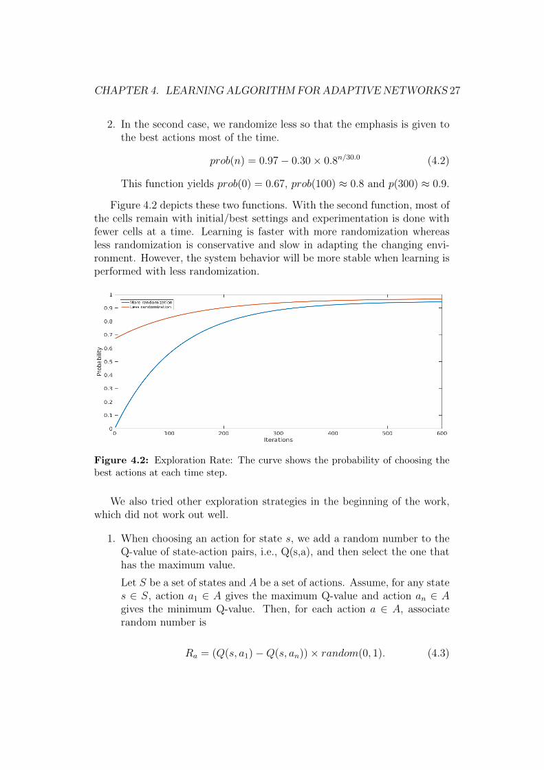
In this section, we discuss the exploration and exploitation policy used inour learning algorithm. In mobile network management, our main objectiveis to improve the connection quality of mobile terminals and this is knownfrom the CQI vector. Hence, the objective here is to move the terminalsfrom lower CQI classes to higher classes. In reinforcement learning, we havethe choice between taking the best action (according to current information)and maximizing future rewards, and learning more by taking an action witha lower value. Thus, we define an exploration rate in such a way that thealgorithm will have a chance to explore more in the beginning and later itcan focus on maximizing the reward. Hence, according to this explorationfunction, the probability of choosing the best action increases gradually overtime. To be able to adapt to a changing network environment, other actionsthan the best one have to be tried occasionally as well. We experimented withtwo different exploration functions based on the degree of randomization.

1. In the first function, the probability of choosing the best action outrightis zero in the beginning and later it increases. Equation 4.1 is one ofthe ways of defining the exploration function.

prob(n) = 0.95− 0.95× 0.7n/40.0 (4.1)

Here, n is the counter for time step. This function yields prob(0) = 0,prob(100) ≈ 0.5 and p(300) ≈ 0.9.


2. In the second case, we randomize less so that the emphasis is given tothe best actions most of the time.

prob(n) = 0.97− 0.30× 0.8n/30.0 (4.2)

This function yields prob(0) = 0.67, prob(100) ≈ 0.8 and p(300) ≈ 0.9.

Figure 4.2 depicts these two functions. With the second function, most ofthe cells remain with initial/best settings and experimentation is done withfewer cells at a time. Learning is faster with more randomization whereasless randomization is conservative and slow in adapting the changing envi-ronment. However, the system behavior will be more stable when learning isperformed with less randomization.

Figure 4.2: Exploration Rate: The curve shows the probability of choosing thebest actions at each time step.

We also tried other exploration strategies in the beginning of the work,which did not work out well.

1. When choosing an action for state s, we add a random number to theQ-value of state-action pairs, i.e., Q(s,a), and then select the one thathas the maximum value.

Let S be a set of states and A be a set of actions. Assume, for any states ∈ S, action a1 ∈ A gives the maximum Q-value and action an ∈ Agives the minimum Q-value. Then, for each action a ∈ A, associaterandom number is

Ra = (Q(s, a1)−Q(s, an))× random(0, 1). (4.3)


Here, random(0, 1) returns a real number from the range 0 and 1.Then, the best action a ∈ A for state s is the one that maximizesRa +Q(s, a), i.e.,

argmaxa∈A(Q(s, a) +Ra). (4.4)

2. Actions that currently look better are chosen with a higher probability.Algorithm 4 formalizes this method.

Algorithm 4: Exploration

1 r = random()2 if r < thresholdvalue1 then3 Choose best action4 else if thresholdvalue1 ≤ r ≤ thresholdvalue2 then5 Choose second best action6 else7 Choose third best action

4.6 Scoring Function for States and Abstract

States

In order to know how good or bad an action is, we need to map the feedbackgiven by the environment to real values. This mapping is defined by a func-tion which we call a scoring function. The scoring function computes a scorefor each state where the state is only a CQI vector and it does not includethe control part. We design the function in such a way that if a successorstate has a better quality of service then the score is higher. Improving theconnection quality of the terminals is more important in lower classes. Thisis because the terminals in higher classes are already in a good state. Hencethe score function is designed accordingly: Moving a terminal from a poorconnection to a good connection improves the score more than moving fromgood to excellent.

We present two different methods for computing the score.

4.6.1 Unabstracted Score

In this case, the scoring function uses the unabstracted CQI vector where thevalues of each CQI class are considered separately. We first define a weight


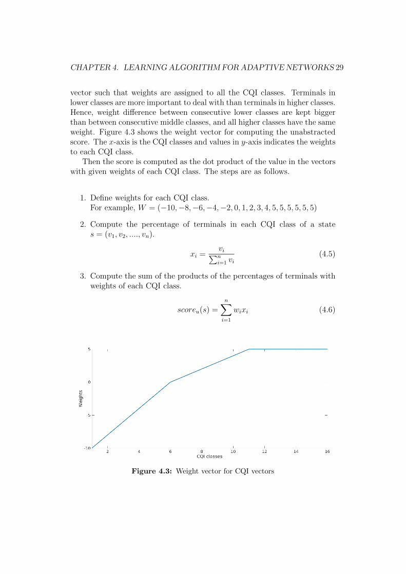
vector such that weights are assigned to all the CQI classes. Terminals inlower classes are more important to deal with than terminals in higher classes.Hence, weight difference between consecutive lower classes are kept biggerthan between consecutive middle classes, and all higher classes have the sameweight. Figure 4.3 shows the weight vector for computing the unabstractedscore. The x-axis is the CQI classes and values in y-axis indicates the weightsto each CQI class.

Then the score is computed as the dot product of the value in the vectorswith given weights of each CQI class. The steps are as follows.

1. Define weights for each CQI class.For example, W = (−10,−8,−6,−4,−2, 0, 1, 2, 3, 4, 5, 5, 5, 5, 5, 5)

2. Compute the percentage of terminals in each CQI class of a states = (v1, v2, ...., vn).

xi =vi∑ni=1 vi

(4.5)

3. Compute the sum of the products of the percentages of terminals withweights of each CQI class.

scoreu(s) =n∑

i=1

wixi (4.6)

Figure 4.3: Weight vector for CQI vectors


4.6.2 Abstracted Score

We also define the score on the basis of abstraction mentioned in Section 4.3.The reason behind using this approach is that it enables to handle all stateabstraction at one point in the interface between learning algorithm and thenetwork. Since, the abstracted states are defined from the CQI vector, scorecan be given directly to abstracted states rather than individual CQI classeswhich prevents multi-processing of the CQI vector. Here, we first definea weight for each CQI component instead of all the CQI classes as in theunabstracted case. Next, the abstracted value of each component is mappedto a real value. Finally, we sum the product of weights with the mappedvalue.

Initially, we chose a linear weight vector to compute the abstracted score.Later, we derived weights as the mean of weights from the unabstractedweight vector which gives the weight vector in piecewise linear form. Forexample, if the number of components is three, then the weight of the firstcomponent is the average value of weights of classes belonging to the firstcomponent. We experimented with both linear and non-linear weight vectorsand the results of comparisons can be found in the experimental part of thisthesis. Figure 4.4 shows the two types of weight vectors used for computingthe abstracted score. Here, we assume that there are eight components intotal and the numbers in y-axis represent the weights of each component.

Figure 4.4: Weight vectors for abstracted states

Equations 4.7 and 4.8 represent the two different scoring functions withlinear and non-linear weights respectively. Here, W1 is a vector of linearweights and W2 is a vector of non-linear weights. The lengths of both ofthese vectors are equal to the number of components. Here, s is a CQI


vector and abstract(s) returns real numbers for abstracted values of the CQIvector.

scorea1(s) = W1 · abstract(s) (4.7)

scorea2(s) = W2 · abstract(s) (4.8)

Example: Assume the CQI classes are divided into three components,poorConnection, goodConnection, and excConnection and each of these com-ponents is mapped to values val1, val2, and val3. Assume the weights areassigned in a linear fashion to the components and if val1 is mapped to 0,val2 to 1, and val3 to 2, then the scoring function in this scenario is,score = 1× poorConnection+ 2× goodConnection+ 3× excConnection= 1× val1 + 2× val2 + 3× val3 = 1× 0 + 2× 1 + 3× 2 = 8.

Mapping from abstracted value The abstracted value is mapped toa real number which is then used in the scoring function to compute the score.In our experiments, we initially mapped these abstracted values in a linearfashion in all the components. Later, we used the proportion of terminalsfalling in the range of each abstracted value. So, the same abstracted value,for example, val1 in the bad component is different than the val1 in theexcellent component and mapping to same real value may not provide abetter estimation of score. To derive the appropriate value we follow theprocess of threshold derivation explained in Subsection 4.3.2 where we havea range of real values for each abstracted value and the median of the rangeof the values is used as the mapping value for score computation. We carriedout the experiments both with linear mapped values and median values andcomparisons will be carried out in the experimental section.

4.7 Rewards for Actions

Given an action a that takes a state s to a new state s′, the reward for theaction a can either be the score of new state s′ or the difference between thescore of successor state s′ and current state s. We used both unabstractedand abstracted scoring functions to compute the reward for actions.

Equation 4.9 defines the reward computed using the score of unabstractedstate. In this case, the reward is the score of new state s′.

Ru(s, s′) = scoreu(s′) (4.9)


Equation 4.10 defines the reward which is also obtained using unab-stracted score, but in this case the reward is the difference between thescore of the successor state s′ and the current state s. In this case, the un-abstracted score is computed for each CQI vector and the reward is the dif-ference of scores of current CQI vector and the previous CQI vector. Hence,if the score is better in current situation than in the previous situation thenthe reward will be positive and otherwise it is negative.

Rdu(s, s′) = scoreu(s′)− scoreu(s) (4.10)

Further, the reward defined by Equation 4.11 is based on the abstractedscore of new state s′ and in this case the scoring function uses linear weightvectors.

Ra1(s, s′) = scorea1(s

′) (4.11)

Equation 4.12 defines another way of computing reward where the ab-stracted score is obtained using non-linear weights.

Ra2(s, s′) = scorea2(s

′) (4.12)

4.8 Q-Value Updates

The next important part of the learning algorithm is updating the Q-valuetable. The Q-value update for each state-action pair (s, a) is defined byEquation 4.13 where the current state is s and taking action a leads to a newstate s′:

Q′(s, a) := γ ×Q(s, a) + (1− γ)×R(s, s′). (4.13)

Here, γ is a constant determining the speed of learning, i.e., the impact ofnew information on Q(s, a) value typically in the range 0.95 < γ < 1. Thereward for action a when it changes the state from s to s′ is R(s, s′), and thepossible ways of computing it were just discussed in Section 4.7.

The update function is simpler than in standard Q-learning because futurerewards do not need to be considered, due to the simple structure of the statespace. Future rewards only depend on the respective future actions, not onthe current action.


4.8.1 Choice of γ

Deciding the value of γ is another important task in the Q-learning algorithm.If γ is constant, then either learning is too slow initially or there is too muchnoise in the Q-values. Hence, in order to make its value dynamic, we countthe number of times the state-action pair appears in the learning process anddefine γ as

γ = 1− 1

min(count(s, a), 100). (4.14)

Here, s is a state and a is an action. So, if a state-action pair appears for thefirst time, then the value of γ is 0 and later the value of γ increases. Thisway the Q-values initially change quickly and after several learning steps thechange will be slower. Figure 4.5 shows γ as a function of count(s, a).

Figure 4.5: Curve showing γ

Chapter 5

Experiments and Results

In this chapter, we study the applicability of our methods by performingexperiments and we try to answer the following questions.

1. How much does learning improve network performance?

2. What kind of abstraction of states is best?

3. How randomization in action selection affects learning?

5.1 Setting

We used a software simulator for mobile networks that was developed byNokia to carry out the experiments. This simulated network consists of 12LTE macro cell base stations and 32 cells in total. We used about 2000terminals moving at random around the simulation area which is an urbanarea in central Helsinki. The network structure and positioning of the cells isshown in the screen-shot in Figure 5.1. The simulator at first runs with initialtransmission settings and it produces the data such as CQI and RLF valuesin every 15 minutes interval of time and the parameter changes are madeafter each measurement round. The CQI vectors produced by the simulatorhad 16 classes.

34

CHAPTER 5. EXPERIMENTS AND RESULTS 35

Figure 5.1: A screen-shot of the LTE network simulator

The initial TXP value for all cells is 40.0. We defined three actions,increment TXP value, decrement TXP value, and no change. Initially, wetried to increase and decrease the TXP by a small value, for example 1 or2. However, the impact of such small TXP changes had negligible impact onnetwork performance. Moreover, too small changes in the TXP values wouldincrease the size of state space. For example, if the range of TXP value isbetween 0 to 40 then changing the value by 1 would generate 40 differentTXP values and each is consider as a unique state. On the other hand, toobig change will make the network unstable. Hence, we decided to changethe value by 4 after some experimentation. This defines the action space as{−4, 0, 4}.

The minimum and maximum TXP values for each cell were also fixedto constant values 0.0 and 40.0, respectively. The switching from one TXPstate to another should remain within these minimum and maximum values.

The whole learning algorithm was developed as a Python program. Wehad a separate class for reading and processing the data produced by thesimulator, and writing the TXP changes in the format so that the simulatorcan read the changes. In addition, the important components of the learningalgorithm such as abstraction, exploration, and Q-value update are imple-mented by separate procedures. The whole code is of around 1100 lines. Thesimulator produces the data after every 15 minutes of interval and hence, thealgorithm needs to wait unless it gets a data based on new TXP changes.


Due to this, running the algorithm for further simulations takes more time.

5.2 Experiments

We performed around 500 simulations for each experiment, and producedresults with all versions of the scoring function. We experimented with thefollowing aspects of the learning algorithm.

• Different levels of abstraction

• Different ways of computing scores

• Variations in exploration policy

• Linear and non-linear weight vectors for computing scores

Basically, we classified the experiments into two categories. The firstcategory involves the experiments performed by changing the number of ab-stracted values (to which each component are mapped to) and the secondone involves the experiments with different number of components.

5.2.1 Base-Line Model

In our base-line model, the base stations’ antenna configuration settings re-main unchanged. We used TXP = 40.0 for all base stations which wassuggested by Nokia as it seems reasonable settings for the base-line model.We tried with other TXP values (30.0 and 25.0) as well but the results arebetter with TXP value, 40.0.

5.2.2 Different Number of Abstract Values

We ran the RL-algorithm with two, three, four, six, and eight abstractedvalues keeping the number of components constant in all cases. We used allthe three reward functions (Ru, Rd

u, and Ra1) for this comparison. Figures5.2, 5.3, and 5.4 show scores during the learning process where the rewardwas computed using the functions Ru, Rd

u, and Ra1 , respectively. In all threeapproaches, the score is increasing and improves on the base-line model. InRd

u , learning with 8 abstracted values is performing well; in Ru, both 3 and8 abstracted values look better, and in Ra1 , the difference is not clear. Weanticipate that this is due to the noise in simulation and also partly due tothe randomization in choosing the actions.


Most of the curves in all three figures initially go down for a certainperiod of time. This is due to the randomization used in exploration. Hence,initially the score decreases, and once the algorithm learns, it starts to selectthe best action with high probability. A more conservative learning strategywith less randomization would avoid this dip in the connection quality.

Figure 5.2: Scores based on different numbers of abstract values with rewardfunction Ru

Figure 5.3: Scores based on different numbers of abstract values with rewardfunction Rd

u


Figure 5.4: Scores based on different numbers of abstract values with rewardfunction Ra1

Figures 5.5 and 5.6 show terminals’ behavior in some of the CQI classeswhen the learning was performed with unabstracted reward, Ru and Rd

u,respectively whereas Figure 5.7 show terminals’ behavior when the learningwas performed with abstracted reward Ra1 . Classes 2 and 3 in Figure 5.5 arelower classes with poor connection quality and there is a slight decrease inthe number of terminals. On the other hand, classes 9, 10, 11, 12 are higherclasses where the number of terminals is increasing. The situation is similarin other two figures as well. Thus, we can say that the terminals are movingfrom lower classes to higher classes thereby the improving the connectionquality.


Figure 5.5: Change in terminals’ behavior for a selection of CQI classes withreward function Ru

Figure 5.6: Change in terminals’ behavior for a selection of CQI classes withreward function Rd

u


Figure 5.7: Change in terminal’s behavior for a selection of CQI classes withreward function Ra1

5.2.3 Different Numbers of Components

We also experimented with different numbers of components. Figure 5.8shows the score when the abstracted states have two, three, four, and eightcomponents.

Figure 5.8: Score based on different numbers of components with reward functionRa1


The score curve for 8-components is an anomaly since the scores are belowthe base-line model. We are not sure about the reasons for this but we thinkthat this is due to the very large Q-value table which leads to very slowlearning. Here, it is also difficult to say what number of components is thebest as the scores for all of them (except 8-components) are similar.

The class-wise plots with different numbers of components are shown inFigure 5.9. As before, the numbers of terminals are decreasing in lower classesand increasing in higher classes. Learning with 2 components performs well.However, the score curve from Figure 5.8 shows that all scores based on two,three and four components yield similar improvement.

Figure 5.9: Change in terminals’ behavior for a selection of CQI classes withreward function Ra1 . Comparisons are based on different number of components.

5.2.4 Weight Vectors and Randomization in ChoosingActions

In all the above experiments, there is more randomization in choosing thebest action in the beginning. In addition, we used linear weights and linearvalues for computing the abstracted score. Later, we changed the weightvector and used less randomization in choosing the action and experimentedwith reward function Ra2 . In addition, we used non-linear numbers for eachabstracted value while computing the score. Due to less randomization,


the algorithm takes better actions with high probability. Figure 5.10 showsthe scores between the older (Version 1) and newer version (Version 2) of8-components where version 2 has better performance .

Figure 5.10: Scores for the two versions with reward functions Ra1 and Ra2 using8 components

Figure 5.11 shows the terminals’ behavior in two different versions of 8components. The newer version is a bit smoother and better than the olderversion.

Figure 5.11: Class-wise comparisons between the two versions with reward func-tions Ra1 and Ra2 using 8 components


Figures 5.12 and 5.13 show scores for the two cases using 4 values and 3values, respectively.

The main difference between these two versions can be seen in the begin-ning of learning. In the older version, the score curve initially goes down, butin the newer version, this is no longer the case. In Figures 5.10, 5.12, and5.13, the scores for the newer versions start increasing from the beginning incontrast with the older version. This is due to less randomization in choosingthe action. However, learning for both cases is similar afterward.

Figure 5.12: Scores for the two versions with reward functions Ra1 and Ra2 using4 abstracted values

Figure 5.13: Scores for the two versions with reward functions Ra1 and Ra2 using3 abstracted values


5.3 Result Analysis

The curves from most of the experiments are highly fluctuating. This fluc-tuation is due to the noise in the simulation. In addition, the noise is due tothe randomization in choosing TXP settings.

Nevertheless, there is an improvement in the score function in most of ourexperiments which means that the algorithm is gradually finding and usingbetter settings. Moreover, the class-wise plots also show that the terminalsare moving from lower quality classes to higher quality classes. But, on theother hand, the terminals’ behavior does not change much with the base-line model and the experiments show that the RL algorithm is doing better.Hence, in reference to our first question, posted in the beginning of thechapter, learning is effective and the performance of the network is improved.

Furthermore, the results with different levels of abstraction have similarimprovements, and it is difficult to answer our second question and say whichamong them is the best abstraction. Nevertheless, if the algorithm is car-ried out for longer interval then it may be possible to distinguish the bestabstraction.

Our third question was about the randomization in action selection andfrom the results, we found that the change in the degree of randomizationof action selection will change the learning behavior. Hence the performanceof learning will increase if action selection and other learning parameters aredefined in a clever way.

To summarize, we meet our objective of improving the connection qual-ity of terminals and the results answer our questions we had prior to theexperiment.

Chapter 6

Discussion

In Chapter 4 we explained a learning algorithm for configuring the parametersof base stations. In this chapter, we will discuss what are the issues with ourlearning method and how one could deal with these issues in the future. Wewill also discuss other possible extensions and variations that can be done.

6.1 Factors Affecting Learning

The algorithm we used for the thesis work is a basic one and it focused onadjusting TXP settings according to the changing environment. The resultsin the previous chapter showed that the learning algorithm is effective andoutperforms the base-line model. Some of the important factors that affectthe learning are as follows.

Method of abstraction The design space of abstractions is large and con-sists of multiple orthogonal choices such as partitioning CQI vectorand threshold values in abstraction of the partitions of the CQI vectoraccording to the values in the vector components.

Score Computation The next important component in our learning algo-rithm is the scoring function. We defined weights for each CQI classin order to compute the score of states. Terminals in lower classes aremore important in improving network behavior, thus we defined theweight vector accordingly. Other weight vectors could be suggestedby network operators, for example if the connection quality could bequantified in financial terms.

Randomization and Learning Rate The randomization in choosing ac-tions plays another important role in learning. More randomization

45

CHAPTER 6. DISCUSSION 46

means lower rewards in the beginning which may cost more to the sys-tem at the initial stages, but in the long run, the algorithm increasesrewards. On the other hand, less randomization could perform well inthe beginning but with slower learning. Therefore, finding a balancebetween the randomization in choosing actions and the cost considera-tion is an important issue. In addition, tuning the learning parametersis equally important. Learning parameters can be adjusted accordingto what is the expected timescale of changes in the network environ-ment or usage patterns. For example, a low learning rate would adaptto changes that take place over months, and a high learning rate wouldcorrespond to changes over days or weeks.

6.2 Possible Variations and Prospects for Fu-

ture Work

There is room for improvement within our learning algorithm and manypossible variations can be integrated as well. Below we discuss some otherpossible approaches and extensions that can be useful in the learning process.

Joint/Cooperative Apart from a limited form of independent learn-ing, we also tried to perform joint learning by considering the control stateof neighboring cells. We include the TXP values of neighboring cells in thestate space and the actions are taken based on the joint reward. However, themethod is not scalable and results in very large state spaces as the numberof parameters increased when the parameters of other base stations are alsoconsidered. Moreover, the scores we obtained from joint learning were similarto the one from independent learning. However, one can still integrate theparameters of few neighboring cells to define the state space in a clever wayso that there is a balance between state space size and learning performance.There are some scenarios where such joint learning approach can be useful.For example, if a cell in then network is dead (switched off), its neighboringcells can adjust their parameters to reconnect terminals previously connectedto the now inactive base station. Furthermore, the problem of interferenceamong the cells in the network can be better solved when the neighboringcells are taken into account when defining the state space.

Partial Observability The algorithm considered in this thesis workviews the network management problem as a fully observable problem. How-ever, in the mobile network, part of the current state of the system (location

CHAPTER 6. DISCUSSION 47

and movement of mobile terminals) is not directly observable. Standard RLmethods assume full observability. So our method essentially views a par-tially observable problem as fully observable. The implications of this forthe learning approach need to be evaluated thoroughly. Consider a base sta-tion changing its antenna settings to achieve better QoS. The learned policypredicts a certain improvement, but the reality may differ from this, and ifQoS actually got worse, the next action could be to restore the antenna set-tings, leading back to the starting state. With standard fully-observable RLmethods this leads to oscillation between two control states, because noth-ing is remembered from the previous state of the system. The underlyingproblem is that the RL method views the system as fully observable withpartial observability inaccurately (incorrectly) represented as nondetermin-ism/stochasticity of the control actions. In the (inaccurate) fully observablerepresentation it makes sense to repeatedly try and fail with the control ac-tion that seemingly would (at least sometimes) lead to the better antenna set-tings, whereas with the (more accurate) partially observable model it wouldbe recognized that the state of the system differs from the prediction, andthat the system state is not precisely captured by the observations alone. Ex-tensions of RL methods to partial observability have been proposed before.Jaakkola et al. [18] handled learning with partial observability by evaluatingPOMDP policy candidates with a Monte-Carlo simulation. Crites and Barto[13] apply RL to elevator control, a problem that has features not addressedby basic RL methods, including partial observability and multiple agents.

Increased complexity brought in by partial observability decreases thescalability of the learning methods, which is why finding a balance betweenaccuracy of the models and the computational scalability becomes an im-portant issue and this can be one of the extensions of the algorithm in thefuture.

Possible extension with current learning approach Apart fromre-designing the algorithm, one could also do a simple extension in the cur-rent approach. In this work, the learning algorithm only takes the TXPsettings for defining the state and actions, but one could also integrate othernetwork parameters such as antenna tilt to the definition of the state spaceand actions. Integrating more parameters will better distinguish the state ofthe network but on the other hand, will increase the size of state space andthe Q-value table. As a result, learning process slows down. Similarly, onecould integrate RLF (Radio Link Failures) values in the algorithm with theobjective of decreasing the number of lost connections.

Chapter 7

Conclusions

Mobile data traffic is expected to grow more than 500-fold between 2010 and2020 [30]. Due to this, the upcoming 5G networks will have high demandsin terms of speed and connection quality. In addition, there will be a lotmore cells in 5G due to adoption of small cells technology. As a result,manual configuration of the network becomes infeasible and there will bea need for an automated approach so that the network can adapt itself tothe highly changing environment. We presented a multi-agent reinforcementlearning method that automates a part of network management in an efficientway and mitigates the complexity of managing the network in the future.Reinforcement learning is an approach to adaptive control in which learningand control processes are interleaved.

We defined the learning algorithm based on the Q-learning framework.The proposed algorithm views the network as a fully observable system withstochastic transitions from one state to another. The algorithm is composedof components such as state abstraction, exploration policy, and scoring func-tion. The network parameters and the status of the terminals indicate thestate of each cell in the network. However, considering all such informationwill result in very large state spaces. Therefore, we abstracted the state spaceto make it manageable. We used CQI vectors, which summarize terminals’connection quality, for defining the state space, and our abstraction methodinvolves partitioning the CQI vector and mapping each partition into a value.Next, we defined the exploration function so that the algorithm randomizesmore in the beginning of learning.

In reinforcement learning, the agent learns from the feedback of the envi-ronment. We considered three different ways of computing scoring functionswhich represent the feedback. The scores are based on the unabstracted andabstracted CQI vector. In addition, we defined a weight vector for both theCQI vector and its abstracted form.

48

CHAPTER 7. CONCLUSIONS 49

We performed experiments with different methods of score computationby varying the abstracted values, components, and exploration strategies.All our experiments are conducted in a simulated environment. The resultsshow that the learning is effective and performs better than the base-linemodel. The scores are increasing as well as there is an improvement in theconnection quality of the terminals.

In this work, we used the learning algorithm to adjust the TXP values ofthe base stations. Nevertheless, one can also adjust other network parameterssuch as antenna tilt and integrate other key performance indicators such asRLF using the same approach. Apart from this, there is room for extensionin many possible ways in the future. Learning with partial observability,cooperative learning that considers the neighboring base stations are someof the possible approaches that can be implemented in the near future andwe hope the integration of these extensions in our current approach help tosolve the network management problem even more effectively.

Bibliography

[1] Andre, D., and Russell, S. J. State abstraction for programmablereinforcement learning agents. In AAAI/IAAI (2002), pp. 119–125.

[2] Atkeson, C. G., and Santamaria, J. C. A comparison of directand model-based reinforcement learning. In In International Conferenceon Robotics and Automation (1997), IEEE Press, pp. 3557–3564.

[3] Baker, M., Sesia, S., and Toufik, I. LTE-The UMTS Long TermEvolution From Theory to Practice. Chichester: John Wiley & Sons,2011.

[4] Barto, A. G., Bradtke, S. J., and Singh, S. P. Learning toact using real-time dynamic programming. Artificial Intelligence 72, 1(1995), 81–138.

[5] Bellman, R. E. Adaptive control processes: a guided tour. PrincetonUniversity Press, 2015.

[6] Bennis, M., and Niyato, D. A Q-learning based approach to inter-ference avoidance in self-organized femtocell networks. In GLOBECOMWorkshops (GC Wkshps), 2010 IEEE (2010), pp. 706–710.

[7] Bennis, M., Perlaza, S. M., Blasco, P., Han, Z., and Poor,H. V. Self-organization in small cell networks: A reinforcement learn-ing approach. Wireless Communications, IEEE Transactions on 12, 7(2013), 3202–3212.

[8] Bernardo, F., Agustı, R., Perez-Romero, J., and Sallent,O. Distributed spectrum management based on reinforcement learning.In Cognitive Radio Oriented Wireless Networks and Communications,2009. CROWNCOM’09. (2009), pp. 1–6.

50

BIBLIOGRAPHY 51

[9] Brafman, R. I., and Tennenholtz, M. R-max - A general poly-nomial time algorithm for near-optimal reinforcement learning. Journalof Machine Learning Research 3, Oct (2002), 213–231.

[10] Chernogorov, F., Repo, I., Raisanen, V., Nihtila, T., andKurjenniemi, J. Cognitive self-healing system for future mobile net-works. In Wireless Communications and Mobile Computing Conference(IWCMC) (2015), IEEE, pp. 628–633.

[11] Claus, C., and Boutilier, C. The dynamics of reinforcement learn-ing in cooperative multiagent systems. In AAAI/IAAI (1998), pp. 746–752.

[12] Cox, C. An introduction to LTE: LTE, LTE-advanced, SAE and 4Gmobile communications. John Wiley & Sons, 2012.

[13] Crites, R., and Barto, A. Improving elevator performance usingreinforcement learning. In Advances in Neural Information ProcessingSystems 8 (1996), pp. 1017–1023.

[14] Diuk, C., Li, L., and Leffler, B. R. The adaptive k-meteorologistsproblem and its application to structure learning and feature selection inreinforcement learning. In Proceedings of the 26th Annual InternationalConference on Machine Learning (2009), ACM, pp. 249–256.

[15] Galindo-Serrano, A., Giupponi, L., and Auer, G. Distributedfemto-to-macro interference management in multiuser ofdma networks.In Proc. of IEEE 73rd Vehicular Technology Conference (VTC2011-Spring), Workshop on Broadband Femtocell Technologies, Budapest,Hungary (2011), pp. 15–18.

[16] Hamalainen, S., Sanneck, H., and Sartori, C. LTE self-organising networks (SON): network management automation for op-erational efficiency. John Wiley & Sons, 2012.

[17] Hatonen, K. Data mining for telecommunications network log analy-sis. Department of Computer Science, series of publications A, reportA-2009-1. University of Helsinki, 2009.

[18] Jaakkola, T., Singh, S. P., and Jordan, M. I. Reinforcementlearning algorithm for partially observable Markov decision problems.Proceedings of the Advances in Neural Information Processing Systems(1995), 345–352.

BIBLIOGRAPHY 52

[19] Jaksch, T., Ortner, R., and Auer, P. Near-optimal regret boundsfor reinforcement learning. Journal of Machine Learning Research 11,Apr (2010), 1563–1600.

[20] Kaelbling, L. P. Learning in embedded systems. The MIT Press,1993.

[21] Kaelbling, L. P., Littman, M. L., and Moore, A. W. Rein-forcement learning: A survey. Journal of Artificial Intelligence Research4 (1996), 237–285.

[22] Kapetanakis, S., and Kudenko, D. Reinforcement learning of coor-dination in cooperative multi-agent systems. AAAI/IAAI 2002 (2002),326–331.

[23] Katehakis, M. N., and Veinott Jr, A. F. The multi-armed banditproblem: decomposition and computation. Mathematics of OperationsResearch 12, 2 (1987), 262–268.

[24] Kemptner, T., and Tsvetkov, B. T. LTE SON-Function Coordi-nation Concept. Network 101 (2013).

[25] Kumpulainen, P. Anomaly detection for communication networkmonitoring applications. Tampere University of Technology. Publica-tion; 1192 (2014).

[26] Lauer, M., and Riedmiller, M. An algorithm for distributed rein-forcement learning in cooperative multi-agent systems. In Proceedings ofthe Seventeenth International Conference on Machine Learning (2000),pp. 535–542.

[27] Lee, M., Marconett, D., Ye, X., and Yoo, S. B. Cognitivenetwork management with reinforcement learning for wireless mesh net-works. In International Workshop on IP Operations and Management(2007), Springer, pp. 168–179.

[28] Li, H. Multi-agent Q-learning of channel selection in multi-user cogni-tive radio systems: a two by two case. In Systems, Man and Cybernet-ics, 2009. SMC 2009. IEEE International Conference on (2009), IEEE,pp. 1893–1898.

[29] Littman, M. L. Markov games as a framework for multi-agent rein-forcement learning. In Proceedings of the Eleventh International Con-ference on Machine Learning (1994), vol. 157, pp. 157–163.

BIBLIOGRAPHY 53

[30] Nakamura, T., Nagata, S., Benjebbour, A., Kishiyama, Y.,Hai, T., Xiaodong, S., Ning, Y., and Nan, L. Trends in smallcell enhancements in LTE advanced. IEEE Communications Magazine51, 2 (2013), 98–105.

[31] Neto, G. From single-agent to multi-agent reinforcement learning:Foundational concepts and methods. Technical report, Learning TheoryCourse, Instituto de Sistemas e Robotica, Instituto Superior Tecnico,Lisbon, 2005.

[32] Niyato, D., and Hossain, E. Dynamics of network selection in het-erogeneous wireless networks: an evolutionary game approach. IEEEtransactions on vehicular technology 58, 4 (2009), 2008–2017.

[33] Østerbø, O., and Grøndalen, O. Benefits of self-organizing net-works (SON) for mobile operators. Journal of Computer Networks andCommunications 2012 (2012).

[34] Raisanen, V., and Tang, H. Knowledge modeling for conflict detec-tion in self-organized networks. In Mobile Networks and Management.Springer, 2011, pp. 107–119.

[35] Razavi, R., Klein, S., and Claussen, H. Self-optimization of ca-pacity and coverage in LTE networks using a fuzzy reinforcement learn-ing approach. In Personal Indoor and Mobile Radio Communications(PIMRC), 2010 IEEE 21st International Symposium on (2010), IEEE,pp. 1865–1870.

[36] Russell, S., and Norvig, P. Artificial Intelligence: A Modern Ap-proach. Prentice Hall Press, 2009.

[37] Seijen, H., Whiteson, S., and Kester, L. Efficient abstractionselection in reinforcement learning. Computational Intelligence 30, 4(2014), 657–699.

[38] Sutton, R. S., and Barto, A. G. Reinforcement learning: Anintroduction. MIT Press, 1998.

[39] Suutarinen, J. Performance measurements of GSM base station sys-tem. Licentiate’s thesis, Tampere University of Technology, Finland(1994).

[40] Szilagyi, P., and Novaczki, S. An automatic detection and diagno-sis framework for mobile communication systems. Network and ServiceManagement, IEEE Transactions on 9, 2 (2012), 184–197.

BIBLIOGRAPHY 54

[41] Tan, M. Multi-agent reinforcement learning: Independent vs. cooper-ative agents. In Proceedings of the Tenth International Conference onMachine Learning (1993), pp. 330–337.

[42] Thrun, S. The role of exploration in learning control. In Handbook forIntelligent Control: Neural, Fuzzy and Adaptive Approaches, D. Whiteand D. Sofge, Eds. Van Nostrand Reinhold, 1992.

[43] Thrun, S. B. Efficient exploration in reinforcement learning. Technicalreport CMU-CS-9 2-102, Carnegie Mellon University, 1992.

[44] Tokic, M. Adaptive ε-greedy exploration in reinforcement learningbased on value differences. In Annual Conference on Artificial Intelli-gence (2010), Springer, pp. 203–210.

[45] Tokic, M., and Palm, G. Value-difference based exploration: Adap-tive control between epsilon-greedy and softmax. In KI (2011), Springer,pp. 335–346.

[46] Watkins, C. J., and Dayan, P. Q-learning. Machine Learning 8,3-4 (1992), 279–292.

[47] Watkins, C. J. C. H. Learning from delayed rewards. PhD thesis,University of Cambridge, England, 1989.

[48] Weiß, G. Distributed reinforcement learning. Robotics and Au-tonomous Systems 15 (1995), 135–142.

[49] Wiering, M. Multi-agent reinforcement learning for traffic light con-trol. In ICML (2000), pp. 1151–1158.

Documents

Adaptive Learning For Mobile Network Management … Learning For Mobile Network Management ... Adaptive Learning For Mobile Network Management ... BTS Base Transceiver Station