U.S. Fish & Wildlife Service

Adaptive HarvestManagement2015 Hunting Season

AdaptiveHarvestManagement2015 Hunting Season

PREFACE

The process of setting waterfowl hunting regulations is conducted annually in the United States (Blohm 1989).This process involves a number of meetings where the status of waterfowl is reviewed by the agencies re-sponsible for setting hunting regulations. In addition, the U.S. Fish and Wildlife Service (USFWS) publishesproposed regulations in the Federal Register to allow public comment. This document is part of a series ofreports intended to support development of harvest regulations for the 2015 hunting season. Specifically, thisreport is intended to provide waterfowl managers and the public with information about the use of adaptiveharvest management (AHM) for setting waterfowl hunting regulations in the United States. This reportprovides the most current data, analyses, and decision-making protocols. However, adaptive management isa dynamic process and some information presented in this report will differ from that in previous reports.

Citation: U.S. Fish and Wildlife Service. 2015. Adaptive Harvest Management: 2015 Hunting Sea-son. U.S. Department of Interior, Washington, D.C. 63 pp. Available online at http://www.fws.gov/birds/

management/adaptive-harvest-management/publications-and-reports.php

ACKNOWLEDGMENTS

A Harvest Management Working Group (HMWG) comprised of representatives from the USFWS, theU.S. Geological Survey (USGS), the Canadian Wildlife Service (CWS), and the four Flyway Councils (Ap-pendix A) was established in 1992 to review the scientific basis for managing waterfowl harvests. Theworking group, supported by technical experts from the waterfowl management and research communities,subsequently proposed a framework for adaptive harvest management, which was first implemented in 1995.The USFWS expresses its gratitude to the HMWG and to the many other individuals, organizations, andagencies that have contributed to the development and implementation of AHM.

This report was prepared by the USFWS Division of Migratory Bird Management. G. S. Boomer andG. S. Zimmerman were the principal authors. Individuals that provided essential information or otherwiseassisted with report preparation included: P. Devers, N. Zimpfer, T. Sanders, S. Chandler, and M. Gendron.Comments regarding this document should be sent to the Chief, Division of Migratory Bird Management,U.S. Fish & Wildlife Service Headquarters, MS: MB, 5275 Leesburg Pike, Falls Church, VA 22041-3803.

We are grateful for the continuing technical support from our USGS colleagues: F. A. Johnson, M. C. Runge,and J. A. Royle, and acknowledge that information provided by USGS in this report has not received theDirector’s approval and, as such, is provisional and subject to revision.

Cover art: 2014 Federal Duck stamp artist Jennifer Miller’s painting of a pair of ruddy ducks (Oxyurajamaicensis).

2

TABLE OF CONTENTS1 EXECUTIVE SUMMARY 6

2 BACKGROUND 8

3 MALLARD STOCKS AND FLYWAY MANAGEMENT 9

4 MALLARD POPULATION DYNAMICS 104.1 Mid-continent Stock . . . . . . . . . . . . . . . . . . . . . . . . . . . . . . . . . . . . . . . . . 104.2 Eastern Stock . . . . . . . . . . . . . . . . . . . . . . . . . . . . . . . . . . . . . . . . . . . . . 124.3 Western Stock . . . . . . . . . . . . . . . . . . . . . . . . . . . . . . . . . . . . . . . . . . . . 12

5 HARVEST-MANAGEMENT OBJECTIVES 14

6 REGULATORY ALTERNATIVES 156.1 Evolution of Alternatives . . . . . . . . . . . . . . . . . . . . . . . . . . . . . . . . . . . . . . 156.2 Regulation-Specific Harvest Rates . . . . . . . . . . . . . . . . . . . . . . . . . . . . . . . . . 16

7 OPTIMAL REGULATORY STRATEGIES 18

8 APPLICATION OF AHM CONCEPTS TO OTHER STOCKS 208.1 American Black Duck . . . . . . . . . . . . . . . . . . . . . . . . . . . . . . . . . . . . . . . . 208.2 Northern Pintails . . . . . . . . . . . . . . . . . . . . . . . . . . . . . . . . . . . . . . . . . . . 228.3 Scaup . . . . . . . . . . . . . . . . . . . . . . . . . . . . . . . . . . . . . . . . . . . . . . . . . 25

9 EMERGING ISSUES IN AHM 26

LITERATURE CITED 28

Appendix A Harvest Management Working Group Members 31

Appendix B 2016 Harvest Management Working Group Priorities 34

Appendix C Mid-continent Mallard Models 35

Appendix D Eastern Mallard Models 39

Appendix E Western Mallard Models 43

Appendix F Modeling Mallard Harvest Rates 49

Appendix G Northern Pintail Models 54

Appendix H Scaup Model 59

3

LIST OF FIGURES1 Survey areas currently assigned to the mid-continent, eastern, and western stocks of mallards

for the purposes of AHM. . . . . . . . . . . . . . . . . . . . . . . . . . . . . . . . . . . . . . . 102 Population estimates of mid-continent mallards observed in the WBPHS (strata: 13–18, 20–50,

and 75–77) and the Great Lakes region (Michigan, Minnesota, and Wisconsin) from 1992 to2015. . . . . . . . . . . . . . . . . . . . . . . . . . . . . . . . . . . . . . . . . . . . . . . . . . . 11

3 Top panel: population estimates of mid-continent mallards observed in the WBPHS comparedto mid-continent mallard model set predictions (weighted average based on 2015 model weightupdates) from 1996 to 2015. Bottom panel: mid-continent mallard model weights (SaRw = ad-ditive mortality and weakly density-dependent reproduction, ScRw = compensatory mortalityand weakly density-dependent reproduction, SaRs = additive mortality and strongly density-dependent reproduction, ScRs = compensatory mortality and strongly density-dependent re-production). . . . . . . . . . . . . . . . . . . . . . . . . . . . . . . . . . . . . . . . . . . . . . . 11

4 Population estimates of eastern mallards observed in the northeastern states (AFBWS) andin southern Ontario and Quebec (WBPHS strata 51–54 and 56) from 1990 to 2015. . . . . . . 12

5 Top panel: population estimates of eastern mallards observed in the WBPHS and the AFBWScompared to eastern mallard model set predictions (weighted average based on 2015 modelweight updates) from 2003 to 2015. Error bars represent 95% confidence intervals. Modelweights were not updated in 2013–14. Bottom panel: eastern mallard model weights (SaRw =additive mortality and weakly density-dependent reproduction, ScRw = compensatory mor-tality and weakly density-dependent reproduction, SaRs = additive mortality and stronglydensity-dependent reproduction, ScRs = compensatory mortality and strongly density-dependentreproduction). . . . . . . . . . . . . . . . . . . . . . . . . . . . . . . . . . . . . . . . . . . . . . 13

6 Population estimates of western mallards observed in Alaska (WBPHS strata 1–12) and California-Oregon (state surveys) combined from 1992 to 2015. . . . . . . . . . . . . . . . . . . . . . . . 14

7 Functional form of the harvest parity constraint designed to allocate allowable black duckharvest equally between the U.S. and Canada. Where p is the proportion of harvest allocatedto one country, and u is the utility of a specific combination of country-specific harvest optionsin achieving the objective of black duck adaptive harvest management. . . . . . . . . . . . . . 21

8 Predictive harvest rate distributions for adult male black ducks expected under the applicationof the 2015-2016 regulatory alternatives in Canada (left) and the U.S. (right). . . . . . . . . . 22

G.1 Harvest yield curves resulting from an equilibrium analysis of the northern pintail model setbased on 2015 model weights. . . . . . . . . . . . . . . . . . . . . . . . . . . . . . . . . . . . . 58

4

LIST OF TABLES1 Regulatory alternatives for the 2015 duck-hunting season. . . . . . . . . . . . . . . . . . . . . 162 Predictions of harvest rates of adult, male, mid-continent, eastern, and western mallards ex-

pected with application of the 2015 regulatory alternatives in the Mississippi and Central,Atlantic, and Pacific Flyways. . . . . . . . . . . . . . . . . . . . . . . . . . . . . . . . . . . . . 17

3 Optimal regulatory strategy for the Mississippi and Central Flyways for the 2015 hunting season. 194 Optimal regulatory strategy for the Atlantic Flyway for the 2015 hunting season. . . . . . . . 195 Optimal regulatory strategy for the Pacific Flyway for the 2015 hunting season. . . . . . . . . 206 Black duck optimal regulatory strategies for Canada and the United States for the 2015 hunting

season. . . . . . . . . . . . . . . . . . . . . . . . . . . . . . . . . . . . . . . . . . . . . . . . . . 237 Substitution rules in the Central and Mississippi Flyways for joint implementation of northern

pintail and mallard harvest strategies. . . . . . . . . . . . . . . . . . . . . . . . . . . . . . . . 248 Northern pintail optimal regulatory strategy for all 4 Flyways for the 2015 hunting season. . . 259 Scaup regulatory alternatives corresponding to the restrictive, moderate, and liberal packages. 2610 Optimal scaup harvest levels and corresponding breeding population sizes for the 2015 hunting

season. . . . . . . . . . . . . . . . . . . . . . . . . . . . . . . . . . . . . . . . . . . . . . . . . . 27C.1 Estimates (N) and associated standard errors (SE) of mid-continent mallards (in millions) ob-

served in the WBPHS (strata 13–18, 20–50, and 75–77) and the Great Lakes region (Michigan,Minnesota, and Wisconsin) from 1992 to 2015. . . . . . . . . . . . . . . . . . . . . . . . . . . 35

D.1 Estimates (N) and associated standard errors (SE) of eastern mallards (in millions) observedin the northeastern U.S. (AFBWS) and southern Ontario and Quebec (WBPHS strata 51–54and 56) from 1990 to 2015. . . . . . . . . . . . . . . . . . . . . . . . . . . . . . . . . . . . . . 39

E.1 Estimates (N) and associated standard errors (SE) of western mallards (in millions) observedin Alaska (WBPHS strata 1–12) from 1990 to 2015 and California-Oregon (state surveys)combined from 1992 to 2015. . . . . . . . . . . . . . . . . . . . . . . . . . . . . . . . . . . . . 43

E.2 Estimates of model parameters resulting from fitting a discrete logistic model with MCMC toa time-series of estimated population sizes and harvest rates of mallards breeding in Alaskafrom 1992 to 2014. . . . . . . . . . . . . . . . . . . . . . . . . . . . . . . . . . . . . . . . . . . 47

E.3 Estimates of model parameters resulting from fitting a discrete logistic model with MCMC toa time-series of estimated population sizes and harvest rates of mallards breeding in Californiaand Oregon from 1992 to 2014. . . . . . . . . . . . . . . . . . . . . . . . . . . . . . . . . . . . 48

F.1 Parameter estimates for predicting mid-continent mallard harvest rates resulting from a hier-archical, Bayesian analysis of mid-continent mallard banding and recovery information from1998 to 2014. . . . . . . . . . . . . . . . . . . . . . . . . . . . . . . . . . . . . . . . . . . . . . 50

F.2 Parameter estimates for predicting eastern mallard harvest rates resulting from a hierarchical,Bayesian analysis of eastern mallard banding and recovery information from 2002 to 2014. . . 52

F.3 Parameter estimates for predicting western mallard harvest rates resulting from a hierarchical,Bayesian analysis of western mallard banding and recovery information from 2008 to 2014. . . 53

G.1 Total pintail harvest expected from the set of regulatory alternatives specified for each Flywayunder the northern pintail adaptive harvest management protocol. . . . . . . . . . . . . . . . 56

H.1 Model parameter estimates resulting from a Bayesian analysis of scaup breeding population,harvest, and banding information from 1974 to 2014. . . . . . . . . . . . . . . . . . . . . . . . 62

5

1 EXECUTIVE SUMMARY

In 1995 the U.S. Fish and Wildlife Service (USFWS) implemented the Adaptive Harvest Management (AHM)program for setting duck hunting regulations in the United States. The AHM approach provides a frameworkfor making objective decisions in the face of incomplete knowledge concerning waterfowl population dynamicsand regulatory impacts.

The AHM protocol is based on the population dynamics and status of three mallard (Anas platyrhynchos)stocks. Mid-continent mallards are defined as those breeding in the Waterfowl Breeding Population andHabitat Survey (WBPHS) strata 13–18, 20–50, and 75–77 plus mallards breeding in the states of Michigan,Minnesota, and Wisconsin (state surveys). The prescribed regulatory alternative for the Mississippi andCentral Flyways depends exclusively on the status of these mallards. Eastern mallards are defined as thosebreeding in WBPHS strata 51–54 and 56 and breeding in the states of Virginia northward into New Hampshire(Atlantic Flyway Breeding Waterfowl Survey [AFBWS]). The regulatory choice for the Atlantic Flywaydepends exclusively on the status of these mallards. Western mallards are defined as those birds breeding inWBPHS strata 1–12 (hereafter Alaska) and those birds breeding in the states of California and Oregon (statesurveys). The regulatory choice for the Pacific Flyway depends exclusively on the status of these mallards.

Mallard population models are based on the best available information and account for uncertainty in popula-tion dynamics and the impact of harvest. Model-specific weights reflect the relative confidence in alternativehypotheses and are updated annually using comparisons of predicted to observed population sizes. For mid-continent mallards, current model weights favor the weakly density-dependent reproductive hypothesis (99%)and the additive-mortality hypothesis (70%). For eastern mallards, current model weights favor the weaklydensity-dependent reproductive hypothesis (73%) and the additive-mortality hypothesis (76%). Unlike mid-continent and eastern mallards, we consider a single functional form to predict western mallard populationdynamics but consider a wide range of parameter values each weighted relative to the support from the data.

For the 2015 hunting season, the USFWS is considering the same regulatory alternatives as last year. Thenature of the restrictive, moderate, and liberal alternatives has remained essentially unchanged since 1997,except that extended framework dates have been offered in the moderate and liberal alternatives since 2002.Harvest rates associated with each of the regulatory alternatives have been updated based on preseasonband-recovery data. The expected harvest rates of adult males under liberal hunting seasons are 0.11 (SD =0.02), 0.14 (SD = 0.04), and 0.12 (SD = 0.03) for mid-continent, eastern, and western mallards, respectively.

Optimal regulatory strategies for the 2015 hunting season were calculated using: (1) harvest-managementobjectives specific to each mallard stock; (2) the 2015 regulatory alternatives; and (3) current populationmodels. Based on this year’s survey results of 11.79 million mid-continent mallards, 4.15 million ponds inPrairie Canada, 0.73 million eastern mallards, and 0.73 million western mallards observed in Alaska (0.47million) and California-Oregon (0.26 million), the optimal choice for all four flyways is the liberal regulatoryalternative.

AHM concepts and tools have been successfully applied toward the development of formal adaptive harvestmanagement protocols that inform American black duck (Anas rubripes), northern pintail (Anas acuta), andscaup (Aythya affinis, A. marila) harvest decisions.

For black ducks, the optimal country-specific regulatory strategies for the 2015 hunting season were calculatedin September 2014 using: (1) an objective to achieve 98% of long-term cumulative harvest, (2) current country-specific black duck regulatory alternatives, and (3) current parameter estimates and model weights. Basedon the 2014 survey results of 0.62 million breeding black ducks and 0.45 million breeding mallards in the coresurvey area, the optimal regulatory choices are the liberal regulatory alternative in Canada and the restrictiveregulatory alternative in the U.S.

For pintails, optimal regulatory strategies for the 2015 hunting season were calculated using: (1) an objectiveof maximizing long-term cumulative harvest, including a closed-season constraint of 1.75 million birds, (2)current pintail regulatory alternatives, and (3) current population models and their relative weights. Based

6

on this year’s survey results of 3.04 million pintails observed at a mean latitude of 55.9 degrees, the optimalregulatory choice for all four Flyways is the liberal regulatory alternative with a 2-bird daily bag limit.

For scaup, optimal regulatory strategies for the 2015 hunting season were calculated using: (1) an objective toachieve 95% of long term cumulative harvest, (2) current scaup regulatory alternatives, and (3) updated modelparameters and weights. Based on this year’s survey results of 4.40 million scaup, the optimal regulatorychoice for all four Flyways is the moderate regulatory alternative.

7

2 BACKGROUND

The annual process of setting duck-hunting regulations in the United States is based on a system of resourcemonitoring, data analyses, and rule-making (Blohm 1989). Each year, monitoring activities such as aerialsurveys and hunter questionnaires provide information on population size, habitat conditions, and harvestlevels. Data collected from this monitoring program are analyzed each year, and proposals for duck-huntingregulations are developed by the Flyway Councils, States, and USFWS. After extensive public review, theUSFWS announces regulatory guidelines within which States can set their hunting seasons.

In 1995, the USFWS adopted the concept of adaptive resource management (Walters 1986) for regulatingduck harvests in the United States. This approach explicitly recognizes that the consequences of huntingregulations cannot be predicted with certainty and provides a framework for making objective decisions inthe face of that uncertainty (Williams and Johnson 1995). Inherent in the adaptive approach is an awarenessthat management performance can be maximized only if regulatory effects can be predicted reliably. Thus,adaptive management relies on an iterative cycle of monitoring, assessment, and decision-making to clarifythe relationships among hunting regulations, harvests, and waterfowl abundance.

In regulating waterfowl harvests, managers face four fundamental sources of uncertainty (Nichols et al. 1995a,Johnson et al. 1996, Williams et al. 1996):

(1) environmental variation – the temporal and spatial variation in weather conditions and other keyfeatures of waterfowl habitat; an example is the annual change in the number of ponds in the PrairiePothole Region, where water conditions influence duck reproductive success;

(2) partial controllability – the ability of managers to control harvest only within limits; the harvest resultingfrom a particular set of hunting regulations cannot be predicted with certainty because of variation inweather conditions, timing of migration, hunter effort, and other factors;

(3) partial observability – the ability to estimate key population attributes (e.g., population size, reproduc-tive rate, harvest) only within the precision afforded by extant monitoring programs; and

(4) structural uncertainty – an incomplete understanding of biological processes; a familiar example isthe long-standing debate about whether harvest is additive to other sources of mortality or whetherpopulations compensate for hunting losses through reduced natural mortality. Structural uncertaintyincreases contentiousness in the decision-making process and decreases the extent to which managerscan meet long-term conservation goals.

AHM was developed as a systematic process for dealing objectively with these uncertainties. The key com-ponents of AHM include (Johnson et al. 1993, Williams and Johnson 1995):

(1) a limited number of regulatory alternatives, which describe Flyway-specific season lengths, bag limits,and framework dates;

(2) a set of population models describing various hypotheses about the effects of harvest and environmentalfactors on waterfowl abundance;

(3) a measure of reliability (probability or “weight”) for each population model; and

(4) a mathematical description of the objective(s) of harvest management (i.e., an “objective function”),by which alternative regulatory strategies can be compared.

These components are used in a stochastic optimization procedure to derive a regulatory strategy. A regula-tory strategy specifies the optimal regulatory choice, with respect to the stated management objectives, foreach possible combination of breeding population size, environmental conditions, and model weights (Johnsonet al. 1997). The setting of annual hunting regulations then involves an iterative process:

8

(1) each year, an optimal regulatory choice is identified based on resource and environmental conditions,and on current model weights;

(2) after the regulatory decision is made, model-specific predictions for subsequent breeding population sizeare determined;

(3) when monitoring data become available, model weights are increased to the extent that observations ofpopulation size agree with predictions, and decreased to the extent that they disagree; and

(4) the new model weights are used to start another iteration of the process.

By iteratively updating model weights and optimizing regulatory choices, the process should eventuallyidentify which model is the best overall predictor of changes in population abundance. The process is optimalin the sense that it provides the regulatory choice each year necessary to maximize management performance.It is adaptive in the sense that the harvest strategy evolves to account for new knowledge generated by acomparison of predicted and observed population sizes.

3 MALLARD STOCKS AND FLYWAY MANAGEMENT

Since its inception AHM has focused on the population dynamics and harvest potential of mallards, espe-cially those breeding in mid-continent North America. Mallards constitute a large portion of the total U.S.duck harvest, and traditionally have been a reliable indicator of the status of many other species. Geo-graphic differences in the reproduction, mortality, and migrations of mallard stocks suggest that there maybe corresponding differences in optimal levels of sport harvest. The ability to regulate harvests of mallardsoriginating from various breeding areas is complicated, however, by the fact that a large degree of mixingoccurs during the hunting season. The challenge for managers, then, is to vary hunting regulations amongFlyways in a manner that recognizes each Flyway’s unique breeding-ground derivation of mallards. Of course,no Flyway receives mallards exclusively from one breeding area; therefore, Flyway-specific harvest strategiesideally should account for multiple breeding stocks that are exposed to a common harvest.

The optimization procedures used in AHM can account for breeding populations of mallards beyond the mid-continent region, and for the manner in which these ducks distribute themselves among the Flyways during thehunting season. An optimal approach would allow for Flyway-specific regulatory strategies, which representan average of the optimal harvest strategies for each contributing breeding stock weighted by the relativesize of each stock in the fall flight. This joint optimization of multiple mallard stocks requires: (1) modelsof population dynamics for all recognized stocks of mallards; (2) an objective function that accounts forharvest-management goals for all mallard stocks in the aggregate; and (3) decision rules allowing Flyway-specific regulatory choices. At present, however, a joint optimization of western, mid-continent, and easternstocks is not feasible due to computational hurdles. However, our preliminary analyses suggest that the lackof a joint optimization does not result in a significant decrease in performance.

Currently, three stocks of mallards are officially recognized for the purposes of AHM (Figure 1). We use aconstrained approach to the optimization of these stocks’ harvest, in which the Atlantic Flyway regulatorystrategy is based exclusively on the status of eastern mallards, the regulatory strategy for the Mississippiand Central Flyways is based exclusively on the status of mid-continent mallards, and the Pacific Flywayregulatory strategy is based exclusively on the status of western mallards.

9

Figure 1 – Survey areas currently assigned to the mid-continent, eastern, and western stocks of mallards for thepurposes of AHM.

4 MALLARD POPULATION DYNAMICS

4.1 Mid-continent Stock

Mid-continent mallards are defined as those breeding in WBPHS strata 13–18, 20–50, and 75–77, and inthe Great Lakes region (Michigan, Minnesota, and Wisconsin; see Figure 1). Estimates of the size of thispopulation are available since 1992, and have varied from 6.3 to 11.8 million (Table C.1, Figure 2). Es-timated breeding-population size in 2015 was 11.79 million (SE = 0.36 million), including 11.17 million(SE = 0.36 million) from the WBPHS and 0.62 million (SE = 0.05 million) from the Great Lakes region.

Details describing the set of population models for mid-continent mallards are provided in Appendix C.The set consists of four alternatives, formed by the combination of two survival hypotheses (additive vs.compensatory hunting mortality) and two reproductive hypotheses (strongly vs. weakly density dependent).Relative weights for the alternative models of mid-continent mallards changed little until all models under-predicted the change in population size from 1998 to 1999, perhaps indicating there is a significant factoraffecting population dynamics that is absent from all four models (Figure 3). Updated model weights suggest apreference for the additive-mortality models (70%) over those describing hunting mortality as compensatory(30%). For most of the time frame, model weights have strongly favored the weakly density-dependentreproductive models over the strongly density-dependent ones, with current model weights of 99% and 1%,respectively. The reader is cautioned, however, that models can sometimes make reliable predictions ofpopulation size for reasons having little to do with the biological hypotheses expressed therein (Johnson et al.2002b).

10

46

810

12

Year

●●

●

●●

●

●

●

●

●●

●

●

●

●

●

●

●●

●

● ●●

●

●

TotalWBPHS

Pop

ulat

ion

Siz

e (m

illio

ns)

1995 2000 2005 2010 2015

0.6

0.8

1.0

1.2

YearYear

Great Lakes

Figure 2 – Population estimates of mid-continent mallards observed in the WBPHS (strata: 13–18, 20–50,and 75–77) and the Great Lakes region (Michigan, Minnesota, and Wisconsin) from 1992 to 2015. Error barsrepresent one standard error.

67

89

1012

Year

Pop

ulat

ion

Siz

e (m

illio

ns)

●●

●

●

●

●

●●

●

●

●

●

●

●

●●

●

● ●●

●

●●

●

●

●

●

●

●

●

● ●

●

●

●

● ●

●

●●

●

●

●

ObservedPredicted

1995 2000 2005 2010 2015

0.0

0.2

0.4

0.6

Year

Mod

el W

eigh

ts

● ● ● ●

● ● ● ●● ● ● ● ● ● ● ● ● ●

● ● ●

●

SaRwScRwSaRsScRs

Year

Figure 3 – Top panel: population estimates of mid-continent mallards observed in the WBPHS compared tomid-continent mallard model set predictions (weighted average based on 2015 model weight updates) from 1996to 2015. Error bars represent 95% confidence intervals. Bottom panel: mid-continent mallard model weights(SaRw = additive mortality and weakly density-dependent reproduction, ScRw = compensatory mortality andweakly density-dependent reproduction, SaRs = additive mortality and strongly density-dependent reproduction,ScRs = compensatory mortality and strongly density-dependent reproduction). Model weights were assumed tobe equal in 1995.

11

4.2 Eastern Stock

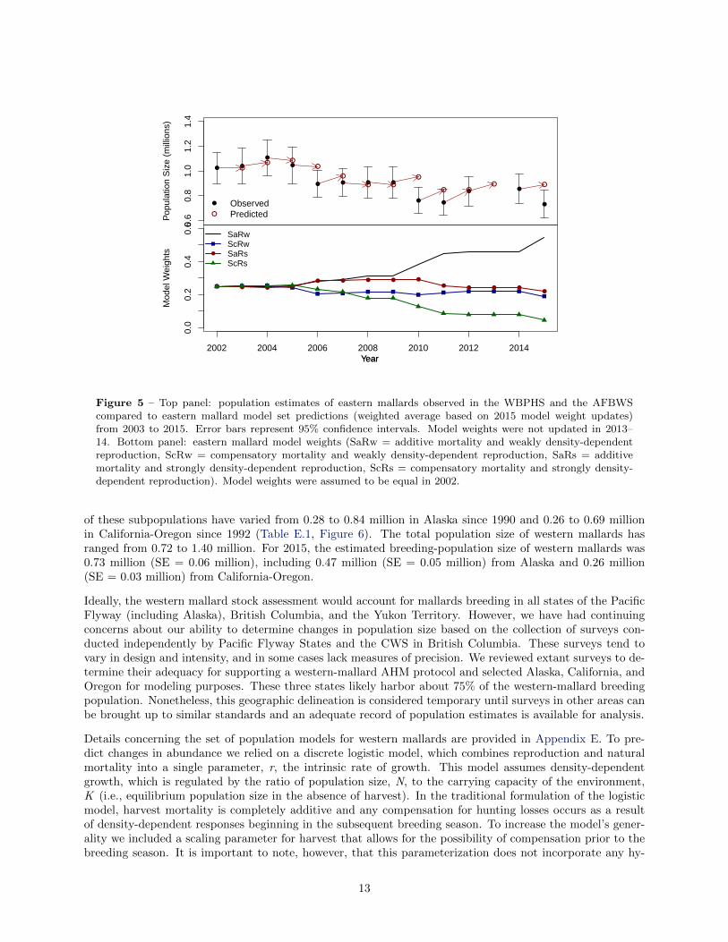
Eastern mallards are defined as those breeding in southern Ontario and Quebec (WBPHS strata 51–54 and56) and in the northeastern U.S.(AFBWS; Heusmann and Sauer 2000, see Figure 1). Estimates of populationsize have varied from 0.73 to 1.1 million since 1990, with the majority of the population accounted for in thenortheastern U.S.(Table D.1, Figure 4). For 2015, the estimated breeding-population size of eastern mallardswas 0.73 million (SE = 0.06 million), including 0.19 million (SE = 0.03 million) from the WBPHS and 0.54million (SE = 0.05 million) from the northeastern U.S.

During the spring of 2013, mechanical problems and corresponding safety concerns with USFWS planeslimited survey coverage of the eastern survey strata in the WBPHS (for more details see U.S. Fish andWildlife Service 2013). Because a 2013 population estimate for the eastern mallard stock was unavailable, welast updated eastern mallard model weights in 2012. As a result, the 2015 model weight updates were basedon this year’s observed BPOP, model predictions based on last year’s observed BPOP, and the 2012 modelweights.

Details describing the population models used for eastern mallard AHM are provided in Appendix D. The setconsists of four alternatives, formed by the combination of two reproductive hypotheses (strongly vs. weaklydensity dependent) and two survival hypotheses (additive vs. compensatory hunting mortality). Modelweights for the eastern mallard model set were computed with a retrospective assessment of relative modelperformance based on the most reliable harvest rate information available from 2002 through 2011. The2015 model weight updates calculated with the eastern mallard model set suggest support for the weaklydensity-dependent reproductive hypothesis 73% and the additive harvest mortality hypothesis 76% (Figure 5).

1990 1995 2000 2005 2010 2015

0.0

0.2

0.4

0.6

0.8

1.0

1.2

1.4

Year

Pop

ulat

ion

Siz

e (m

illio

ns)

●●

●●

●●

●

●

●

●

●

● ●

● ● ●

●●

●●

●●

● ●●

●

TotalAFBWSWBPHS

Figure 4 – Population estimates of eastern mallards observed in the northeastern states (AFBWS) and insouthern Ontario and Quebec (WBPHS strata 51–54 and 56) from 1990 to 2015. In 2013, population estimateswere only available for the northeastern states (AFBWS). Error bars represent one standard error.

4.3 Western Stock

Western mallards consist of 2 substocks and are defined as those birds breeding in Alaska (WBPHS strata1–12) and those birds breeding in California and Oregon (state surveys; see Figure 1). Estimates of the size

12

0.6

0.8

1.0

1.2

1.4

Year

Pop

ulat

ion

Siz

e (m

illio

ns)

● ●

●

●

● ● ● ●

● ●

● ●

●

●● ●

●

●

● ●

●

● ●● ●

●

●

ObservedPredicted

2002 2004 2006 2008 2010 2012 2014

0.0

0.2

0.4

0.6

Year

Mod

el W

eigh

ts

● ● ● ●● ● ● ● ●

● ● ● ●●

●

SaRwScRwSaRsScRs

YearYear

Figure 5 – Top panel: population estimates of eastern mallards observed in the WBPHS and the AFBWScompared to eastern mallard model set predictions (weighted average based on 2015 model weight updates)from 2003 to 2015. Error bars represent 95% confidence intervals. Model weights were not updated in 2013–14. Bottom panel: eastern mallard model weights (SaRw = additive mortality and weakly density-dependentreproduction, ScRw = compensatory mortality and weakly density-dependent reproduction, SaRs = additivemortality and strongly density-dependent reproduction, ScRs = compensatory mortality and strongly density-dependent reproduction). Model weights were assumed to be equal in 2002.

of these subpopulations have varied from 0.28 to 0.84 million in Alaska since 1990 and 0.26 to 0.69 millionin California-Oregon since 1992 (Table E.1, Figure 6). The total population size of western mallards hasranged from 0.72 to 1.40 million. For 2015, the estimated breeding-population size of western mallards was0.73 million (SE = 0.06 million), including 0.47 million (SE = 0.05 million) from Alaska and 0.26 million(SE = 0.03 million) from California-Oregon.

Ideally, the western mallard stock assessment would account for mallards breeding in all states of the PacificFlyway (including Alaska), British Columbia, and the Yukon Territory. However, we have had continuingconcerns about our ability to determine changes in population size based on the collection of surveys con-ducted independently by Pacific Flyway States and the CWS in British Columbia. These surveys tend tovary in design and intensity, and in some cases lack measures of precision. We reviewed extant surveys to de-termine their adequacy for supporting a western-mallard AHM protocol and selected Alaska, California, andOregon for modeling purposes. These three states likely harbor about 75% of the western-mallard breedingpopulation. Nonetheless, this geographic delineation is considered temporary until surveys in other areas canbe brought up to similar standards and an adequate record of population estimates is available for analysis.

Details concerning the set of population models for western mallards are provided in Appendix E. To pre-dict changes in abundance we relied on a discrete logistic model, which combines reproduction and naturalmortality into a single parameter, r, the intrinsic rate of growth. This model assumes density-dependentgrowth, which is regulated by the ratio of population size, N, to the carrying capacity of the environment,K (i.e., equilibrium population size in the absence of harvest). In the traditional formulation of the logisticmodel, harvest mortality is completely additive and any compensation for hunting losses occurs as a resultof density-dependent responses beginning in the subsequent breeding season. To increase the model’s gener-ality we included a scaling parameter for harvest that allows for the possibility of compensation prior to thebreeding season. It is important to note, however, that this parameterization does not incorporate any hy-

13

1995 2000 2005 2010 2015

0.0

0.5

1.0

1.5

Year

Pop

ulat

ion

Siz

e (m

illio

ns)

●

●

●

● ●

●

●

●●

●●

●●

●

●

●●

●

●

●

●

●

●●

●

TotalAKCA−OR

Figure 6 – Population estimates of western mallards observed in Alaska (WBPHS strata 1–12) and California-Oregon (state surveys) combined from 1992 to 2015. Error bars represent one standard error.

pothesized mechanism for harvest compensation and, therefore, must be interpreted cautiously. We modeledAlaska mallards independently of those in California and Oregon because of differing population trajectories(see Figure 6) and substantial differences in the distribution of band recoveries.

We used Bayesian estimation methods in combination with a state-space model that accounts explicitly forboth process and observation error in breeding population size (Meyer and Millar 1999). Breeding populationestimates of mallards in Alaska are available since 1955, but we had to limit the time series to 1990–2014because of changes in survey methodology and insufficient band-recovery data. The logistic model and associ-ated posterior parameter estimates provided a reasonable fit to the observed time series of Alaska populationestimates. The estimated median carrying capacity was 1.00 million and the intrinsic rate of growth was 0.29.The posterior median estimate of the scaling parameter was 1.28, suggesting that harvest mortality may beadditive. Breeding population and harvest-rate data were available for California-Oregon mallards for theperiod 1992–2014. The logistic model also provided a reasonable fit to these data. The estimated mediancarrying capacity was 0.58 million, and the intrinsic rate of growth was 0.26. The posterior median estimateof the scaling parameter was 0.52, suggesting that harvest mortality may be partially compensatory.

The AHM protocol for western mallards is structured similarly to that used for eastern mallards, in which anoptimal harvest strategy is based on the status of a single breeding stock and harvest regulations in a singleflyway. Although the contribution of mid-continent mallards to the Pacific Flyway harvest is significant, webelieve an independent harvest strategy for western mallards poses little risk to the mid-continent stock.Further analyses will be needed to confirm this conclusion, and to better understand the potential effect ofmid-continent mallard status on sustainable hunting opportunities in the Pacific Flyway.

5 HARVEST-MANAGEMENT OBJECTIVES

The basic harvest-management objective for mid-continent mallards is to maximize cumulative harvest overthe long term, which inherently requires perpetuation of a viable population. Moreover, this objective is

14

constrained to avoid regulations that could be expected to result in a subsequent population size below thegoal of the North American Waterfowl Management Plan (NAWMP). According to this constraint, the valueof harvest decreases proportionally as the difference between the goal and expected population size increases.This balance of harvest and population objectives results in a regulatory strategy that is more conservativethan that for maximizing long-term harvest, but more liberal than a strategy to attain the NAWMP goal(regardless of effects on hunting opportunity). The current objective for mid-continent mallards uses apopulation goal of 8.5 million birds, which consists of 7.9 million mallards from the WBPHS (strata 13–18,20–50, and 75–77) corresponding to the mallard population goal in the 1998 update of the NAWMP (less theportion of the mallard goal comprised of birds breeding in Alaska) and a goal of 0.6 million for the combinedstates of Michigan, Minnesota, and Wisconsin.

For eastern and western mallards, there is no NAWMP goal or other established target for desired populationsize. Accordingly, the management objective for eastern and western mallards is to maximize long-termcumulative (i.e., sustainable) harvest.

6 REGULATORY ALTERNATIVES

6.1 Evolution of Alternatives

When AHM was first implemented in 1995, three regulatory alternatives characterized as liberal, moderate,and restrictive were defined based on regulations used during 1979–84, 1985–87, and 1988–93, respectively.These regulatory alternatives also were considered for the 1996 hunting season. In 1997, the regulatoryalternatives were modified to include: (1) the addition of a very-restrictive alternative; (2) additional daysand a higher duck bag limit in the moderate and liberal alternatives; and (3) an increase in the bag limit ofhen mallards in the moderate and liberal alternatives. In 2002, the USFWS further modified the moderateand liberal alternatives to include extensions of approximately one week in both the opening and closingframework dates.

In 2003, the very-restrictive alternative was eliminated at the request of the Flyway Councils. Expectedharvest rates under the very-restrictive alternative did not differ significantly from those under the restrictivealternative, and the very-restrictive alternative was expected to be prescribed for <5% of all hunting seasons.Also in 2003, at the request of the Flyway Councils the USFWS agreed to exclude closed duck-hunting seasonsfrom the AHM protocol when the population size of mid-continent mallards (as defined in 2003: WBPHSstrata 1–18, 20–50, and 75–77 plus the Great Lakes region) was≥5.5 million. Based on our original assessment,closed hunting seasons did not appear to be necessary from the perspective of sustainable harvesting whenthe mid-continent mallard population exceeded this level. The impact of maintaining open seasons above thislevel also appeared negligible for other mid-continent duck species, as based on population models developedby Johnson (2003).

In 2008, the mid-continent mallard stock was redefined to exclude mallards breeding in Alaska, necessitatinga re-scaling of the closed-season constraint. Initially, we attempted to adjust the original 5.5 million closurethreshold by subtracting out the 1985 Alaska breeding population estimate, which was the year upon whichthe original closed season constraint was based. Our initial re-scaling resulted in a new threshold equal to5.25 million. Simulations based on optimal policies using this revised closed season constraint suggested thatthe Mississippi and Central Flyways would experience a 70% increase in the frequency of closed seasons. Atthat time, we agreed to consider alternative re-scalings in order to minimize the effects on the mid-continentmallard strategy and account for the increase in mean breeding population sizes in Alaska over the pastseveral decades. Based on this assessment, we recommended a revised closed season constraint of 4.75 millionwhich resulted in a strategy performance equivalent to the performance expected prior to the re-definition ofthe mid-continent mallard stock. Because the performance of the revised strategy is essentially unchangedfrom the original strategy, we believe it will have no greater impact on other duck stocks in the Mississippiand Central Flyways. However, complete- or partial-season closures for particular species or populations

15

could still be deemed necessary in some situations regardless of the status of mid-continent mallards. Detailsof the regulatory alternatives for each Flyway are provided in Table 1.

6.2 Regulation-Specific Harvest Rates

Harvest rates of mallards associated with each of the open-season regulatory alternatives were initially pre-dicted using harvest-rate estimates from 1979–84, which were adjusted to reflect current hunter numbers andcontemporary specifications of season lengths and bag limits. In the case of closed seasons in the U.S., weassumed rates of harvest would be similar to those observed in Canada during 1988–93, which was a periodof restrictive regulations both in Canada and the U.S. All harvest-rate predictions were based only in part onband-recovery data, and relied heavily on models of hunting effort and success derived from hunter surveys(Appendix C in U.S. Fish and Wildlife Service 2002). As such, these predictions had large sampling variancesand their accuracy was uncertain.

In 2002, we began relying on Bayesian statistical methods for improving regulation-specific predictions ofharvest rates, including predictions of the effects of framework-date extensions. Essentially, the idea is touse existing (prior) information to develop initial harvest-rate predictions (as above), to make regulatorydecisions based on those predictions, and then to observe realized harvest rates. Those observed harvestrates, in turn, are treated as new sources of information for calculating updated (posterior) predictions.Bayesian methods are attractive because they provide a quantitative, formal, and an intuitive approach toadaptive management.

Annual harvest rate estimates for each mallard stock are updated with band-recovery information from acooperative banding program between the USFWS, CWS, along with state, provincial, and other participating

Table 1 – Regulatory alternatives for the 2015 duck-hunting season.

Flyway

Regulation Atlantica Mississippi Centralb Pacificc

Shooting Hours one-half hour before sunrise to sunset

Framework Dates

Restrictive Oct 1–Jan 20 Saturday nearest Oct 1 to the Sunday nearest Jan 20

ModerateSaturday nearest September 24 to the last Sunday in January

Liberal

Season Length (days)

Restrictive 30 30 39 60

Moderate 45 45 60 86

Liberal 60 60 74 107

Bag Limit (total / mallard / hen mallard)

Restrictive 3 / 3 / 1 3 / 2 / 1 3 / 3 / 1 4 / 3 / 1

Moderate 6 / 4 / 2 6 / 4 / 1 6 / 5 / 1 7 / 5 / 2

Liberal 6 / 4 / 2 6 / 4 / 2 6 / 5 / 2 7 / 7 / 2

a The states of Maine, Massachusetts, Connecticut, Pennsylvania, New Jersey, Maryland, Delaware, WestVirginia, Virginia, and North Carolina are permitted to exclude Sundays, which are closed to hunting, fromtheir total allotment of season days.

b The High Plains Mallard Management Unit is allowed 12, 23, and 23 extra days in the restrictive, moderate,and liberal alternatives, respectively.

c The Columbia Basin Mallard Management Unit is allowed seven extra days in the restrictive and moderatealternatives.

16

partners. Recovery rate estimates from these data are adjusted with reporting rate probabilities resultingfrom a recent reward band study from 2002 to 2010 (Boomer et al. 2013). For mid-continent mallards, wehave empirical estimates of harvest rate from the recent period of liberal hunting regulations (1998–2014).Bayesian methods allow us to combine these estimates with our prior predictions to provide updated estimatesof harvest rates expected under the liberal regulatory alternative. Moreover, in the absence of experience(so far) with the restrictive and moderate regulatory alternatives, we reasoned that our initial predictions ofharvest rates associated with those alternatives should be re-scaled based on a comparison of predicted andobserved harvest rates under the liberal regulatory alternative. In other words, if observed harvest rates underthe liberal alternative were 10% less than predicted, then we might also expect that the mean harvest rateunder the moderate alternative would be 10% less than predicted. The appropriate scaling factors currentlyare based exclusively on prior beliefs about differences in mean harvest rate among regulatory alternatives, butthey will be updated once we have experience with something other than the liberal alternative. A detaileddescription of the analytical framework for modeling mallard harvest rates is provided in Appendix F.

Our models of regulation-specific harvest rates also allow for the marginal effect of framework-date extensionsin the moderate and liberal alternatives. A previous analysis by the U.S. Fish and Wildlife Service (2001)suggested that implementation of framework-date extensions might be expected to increase the harvest rate ofmid-continent mallards by about 15%, or in absolute terms by about 0.02 (SD = 0.01). Based on the observedharvest rates during the 2002–2014 hunting seasons, the updated (posterior) estimate of the marginal changein harvest rate attributable to the framework-date extension is 0.006 (SD = 0.007). The estimated effect ofthe framework-date extension has been to increase harvest rate of mid-continent mallards by about 5% overwhat would otherwise be expected in the liberal alternative. However, the reader is strongly cautioned thatreliable inference about the marginal effect of framework-date extensions ultimately depends on a rigorousexperimental design (including controls and random application of treatments).

Current predictions of harvest rates of adult-male mid-continent mallards associated with each of the regu-latory alternatives are provided in Table 2. Predictions of harvest rates for the other age and sex cohorts arebased on the historical ratios of cohort-specific harvest rates to adult-male rates (Runge et al. 2002). Theseratios are considered fixed at their long-term averages and are 1.5407, 0.7191, and 1.1175 for young males,adult females, and young females, respectively. We make the simplifying assumption that the harvest ratesof mid-continent mallards depend solely on the regulatory choice in the Mississippi and Central Flyways.

The predicted harvest rates of eastern mallards are updated in the same fashion as that for mid-continentmallards based on preseason banding conducted in eastern Canada and the northeastern U.S.(Appendix F).Like mid-continent mallards, harvest rates of age and sex cohorts other than adult male mallards are basedon constant rates of differential vulnerability as derived from band-recovery data. For eastern mallards, theseconstants are 1.1534, 1.3306, and 1.5090 for adult females, young males, and young females, respectively(Johnson et al. 2002a). Regulation-specific predictions of harvest rates of adult-male eastern mallards areprovided in Table 2.

In contrast to mid-continent mallards, framework-date extensions were expected to increase the harvest rateof eastern mallards by only about 5% (U.S. Fish and Wildlife Service 2001), or in absolute terms by about

Table 2 – Predictions of harvest rates of adult, male, mid-continent, eastern, and western mallards expectedwith application of the 2015 regulatory alternatives in the Mississippi and Central, Atlantic, and Pacific Flyways.

Mid-continent Eastern Western

Regulatory Alternative Mean SD Mean SD Mean SD

Closed (U.S.) 0.0088 0.0020 0.0792 0.0232 0.0082 0.0182

Restrictive 0.0552 0.0129 0.1063 0.0389 0.0619 0.0173

Moderate 0.0977 0.0215 0.1313 0.0472 0.1034 0.0286

Liberal 0.1139 0.0179 0.1416 0.0360 0.1228 0.0288

17

0.01 (SD = 0.01). Based on the observed harvest rates during the 2002–2014 hunting seasons, the updated(posterior) estimate of the marginal change in harvest rate attributable to the framework-date extension is0.002 (SD = 0.009). The estimated effect of the framework-date extension has been to increase harvest rateof eastern mallards by about 1.3% over what would otherwise be expected in the liberal alternative.

Based on available estimates of harvest rates of mallards banded in California and Oregon during 1990–1995and 2002–2007, there was no apparent relationship between harvest rate and regulatory changes in the PacificFlyway. This is unusual given our ability to document such a relationship in other mallard stocks and in otherspecies. We note, however, that the period 2002–2007 was comprised of both stable and liberal regulationsand harvest rate estimates were based solely on reward bands. Regulations were relatively restrictive duringmost of the earlier period and harvest rates were estimated based on standard bands using reporting ratesestimated from reward banding during 1987–1988. Additionally, 1993–1995 were transition years in whichfull-address and toll-free bands were being introduced and information to assess their reporting rates (andtheir effects on reporting rates of standard bands) is limited. Thus, the two periods in which we wish tocompare harvest rates are characterized not only by changes in regulations, but also in estimation methods.

Consequently, we lack a sound empirical basis for predicting harvest rates of western mallards associatedwith current regulatory alternatives in the Pacific Flyway. In 2009, we began using Bayesian statisticalmethods for improving regulation-specific predictions of harvest rates (see Appendix F). The methodology isanalogous to that currently in use for mid-continent and eastern mallards except that the marginal effect offramework date extensions in moderate and liberal alternatives is inestimable because there are no data priorto implementation of extensions. In 2008, we specified prior regulation-specific harvest rates of 0.01, 0.06, 0.09,and 0.11 with associated standard deviations of 0.003, 0.02, 0.03, and 0.03 for the closed, restrictive, moderate,and liberal alternatives, respectively. The prior for the liberal regulation was then updated in 2011 with aharvest rate of 0.12 and standard deviation of 0.04. The harvest rates for the liberal alternative were based onempirical estimates realized under the current liberal alternative during 2002–2007 and determined from adult-male mallards banded with reward bands and standard bands adjusted for band reporting rates in Californiaand Oregon. Harvest rates for the moderate and restrictive alternatives were based on the proportional (0.85and 0.51) difference in harvest rates expected for mid-continent mallards under the respective alternatives.And finally, harvest rate for the closed alternative was based on what we might realize with a closed season inthe U.S.(including Alaska) and a very restrictive season in Canada, similar to that for mid-continent mallards.A relatively large standard deviation (CV = 0.3) was chosen to reflect greater uncertainty about the meansthan that for mid-continent mallards (CV = 0.2). Current predictions of harvest rates of adult-male westernmallards associated with each regulatory alternative are provided in Table 2.

7 OPTIMAL REGULATORY STRATEGIES

Using stochastic dynamic programming (Lubow 1995, Johnson and Williams 1999), we calculated the optimalregulatory strategy for the Mississippi and Central Flyways based on: (1) the 2015 regulatory alternatives,including the closed-season constraint; (2) current population models and associated weights for mid-continentmallards; and (3) the dual objectives of maximizing long-term cumulative harvest and achieving a populationgoal of 8.5 million mid-continent mallards. The resulting regulatory strategy (Table 3) is similar to that usedlast year. Note that prescriptions for closed seasons in this strategy represent resource conditions that areinsufficient to support one of the current regulatory alternatives, given current harvest-management objectivesand constraints. However, closed seasons under all of these conditions are not necessarily required for long-term resource protection, and simply reflect the NAWMP population goal and the nature of the currentregulatory alternatives. Assuming that regulatory choices adhered to this strategy (and that current modelweights accurately reflect population dynamics), breeding-population size would be expected to average 7.39million (SD = 1.99 million). Based on an estimated population size of 11.79 million mid-continent mallardsand 4.15 million ponds in Prairie Canada, the optimal choice for the Mississippi and Central Flyways in 2015is the liberal regulatory alternative.

We calculated the optimal regulatory strategy for the Atlantic Flyway based on: (1) the 2015 regulatory

18

Table 3 – Optimal regulatory strategya for the Mississippi and Central Flyways for the 2015 hunting season.This strategy is based on current regulatory alternatives (including the closed-season constraint), mid-continentmallard models and weights, and the dual objectives of maximizing long-term cumulative harvest and achievinga population goal of 8.5 million mallards. The shaded cell indicates the regulatory prescription for 2015.

Pondsc

BPOPb 1.5 2.0 2.5 3.0 3.5 4.0 4.5 5.0 5.5 6.0

≤4.5 C C C C C C C C C C

4.75–6.25 R R R R R R R R R R

6.5 R R R R R R R R R M

6.75 R R R R R R R R M M

7 R R R R R R M M M L

7.25 R R R R M M L L L L

7.5 R R M M M L L L L L

7.75 R M M L L L L L L L

8.0 M M L L L L L L L L

≥8.25 L L L L L L L L L L

a C = closed season, R = restrictive, M = moderate, L = liberal.b Mallard breeding population size (in millions) in the WBPHS (strata 13–18, 20–50, 75–77) and Michigan, Minnesota, andWisconsin.

c Ponds (in millions) in Prairie Canada in May.

alternatives; (2) the eastern mallard population models and current model weights; and (3) an objective tomaximize long-term cumulative harvest. The resulting strategy suggests liberal regulations for all populationsizes of record, and is characterized by a lack of intermediate regulations (Table 4). We simulated theuse of this regulatory strategy to determine expected performance characteristics. Assuming that harvestmanagement adhered to this strategy (and that 2015 model weights accurately reflect population dynamics),breeding-population size would be expected to average 1.01 million (SD = 0.31 million). Based on anestimated breeding population size of 0.73 million mallards, the optimal choice for the Atlantic Flyway in2015 is the liberal regulatory alternative.

We calculated the optimal regulatory strategy for the Pacific Flyway based on: (1) the 2015 regulatoryalternatives, (2) current (1990–2014) population models and parameter estimates, and (3) an objective tomaximize long-term cumulative harvest (Table 5). We simulated the use of this regulatory strategy todetermine expected performance characteristics. Assuming that harvest management adhered to this strategy

Table 4 – Optimal regulatory strategya for the Atlantic Flyway for the 2015 hunting season. This strategy isbased on current regulatory alternatives, eastern mallard models and 2015 model weights, and an objective tomaximize long-term cumulative harvest. The shaded cell indicates the regulatory prescription for 2015.

Mallardsb Regulation

≤0.300 C

0.375 R

≥0.400 L

a C = closed season, R = restrictive, L = liberal.b Estimated number of mallards (in millions) in eastern Canada (WBPHS strata 51–54, 56) and the northeasternU.S. (AFBWS).

19

(and that current model parameters accurately reflect population dynamics), breeding-population size wouldbe expected to average 0.96 million (SD = 0.24 million) in Alaska and 0.44 million (SD = 0.03 million) inCalifornia-Oregon. Based on an estimated breeding population size of 0.47 million mallards in Alaska and0.26 million in California-Oregon, the optimal choice for the Pacific Flyway in 2015 is the liberal regulatoryalternative (see Table 5).

Table 5 – Optimal regulatory strategya for the Pacific Flyway for the 2015 hunting season. This strategy isbased on the 2015 regulatory alternatives, current (1990–2014) western mallard population models and parameterestimates, and an objective to maximize long-term cumulative harvest. The shaded cell indicates the regulatoryprescription for 2015.

Alaska BPOPb

CA–OR BPOPb 0 0.05 0.1 0.15 0.2 0.25 0.3 0.35 0.4 0.45 ≥0.5

0 C C C C C C C R L L L

0.05 C C C C C C C C C C C

0.1 C C C C C C C C C R L

0.15 M C C C C C C R L L L

0.2 L C C C C C M L L L L

0.25 L C C C C M L L L L L

0.3 L C C C L L L L L L L

0.35 L C C M L L L L L L L

0.4 L C M L L L L L L L L

0.45 L M L L L L L L L L L

0.5 L M L L L L L L L L L

≥0.55 L L L L L L L L L L L

a C = closed season, R = restrictive, M = moderate, L = liberal.b Estimated number of mallards (in millions) for Alaska (WBPHS strata 1–12) and in California-Oregon.

8 APPLICATION OF AHM CONCEPTS TO OTHER STOCKS

The USFWS is working to apply the principles and tools of AHM to improve decision-making for severalother stocks of waterfowl. Below, we provide the 2015 AHM updates that are currently informing Americanblack duck, northern pintail, and scaup harvest management decisions.

8.1 American Black Duck

Federal, state, and provincial agencies in the U.S. and Canada agreed that an international harvest strategyfor black ducks is needed because the resource is valued by both countries and both countries have theability to influence the resource through harvest. The partners also agreed a harvest strategy should bedeveloped with an AHM approach based on the integrated breeding-ground survey data (Zimmerman et al.2012, U.S. Fish and Wildlife Service 2013). Finally, the strategy should also provide a formal approach todetermining appropriate harvest levels and fair allocation of the harvest between countries (Conroy 2010).

The overall goals of the Black Duck International Harvest strategy include:

(1) maintain a black duck population that meets legal mandates and provides consumptive and non-consumptive use commensurate with habitat carrying capacity;

20

(2) maintain societal values associated with the hunting tradition; and

(3) maintain equitable access to the black duck resource in Canada and the U.S.

The objectives of the harvest strategy are to achieve 98% of the long-term cumulative harvest and to sharethe allocated harvest (i.e., parity) equitably between countries. Historically, the realized allocation of harvestbetween Canada and the U.S. has ranged from 40% to 60% in either country. Recognizing the historicalallocation and acknowledging incomplete control over harvest, parity is achieved through a constraint whichdiscounts combinations of country-specific harvest rates that are expected to result in allocation of harvestthat is >50% in one country. The constraint applies a mild penalty on country-specific harvest optionsthat result in one country receiving >50% but <60% of the harvest allocation and a stronger discount oncombinations resulting in one country receiving >60% of the harvest allocation (Figure 7). The goals andobjectives of the black duck AHM framework were developed through a formal consultation process withrepresentatives from the Canadian Wildlife Service, U.S. Fish and Wildlife Service, Atlantic Flyway Counciland Mississippi Flyway Council.

Country-specific harvest opportunities were determined from a set of expected harvest rate distributions de-fined as regulatory packages. Initially, Canada developed 4 regulatory packages (liberal, moderate, restrictiveand closed) and the U.S. developed 3 (moderate, restrictive, closed), with the Canadian moderate and U.S.restrictive packages defined as 1990–2010 harvest levels (Figure 8). Due to the limited changes in black duckhunting regulations in either country since 1984 specific regulatory frameworks are not currently availablefor restrictive package in Canada or the a moderate package in the U.S. Therefore, the Canadian restrictivepackage is designed to achieve a 30% reduction in mean harvest rate over the 1990-2010 mean harvest rate.Similarly, the moderate packages in the U.S., is designed to achieve a 30% increase in mean harvest rate overthe 1990–2010 mean harvest rate. The closed package would require either country to prohibit black duckharvest. Canada and the U.S. will determine, independently, appropriate regulations designed to achievetheir prescribed harvest targets as identified under the regulatory packages. Regulations will vary indepen-dently between countries based on the status of the population and optimal strategy as determined throughthe AHM protocol.

Figure 7 – Functional form of the harvest parity constraint designed to allocate allowable black duck harvestequally between the U.S. and Canada. Where p is the proportion of harvest allocated to one country, and u isthe utility of a specific combination of country-specific harvest options in achieving the objective of black duckadaptive harvest management.

21

The AHM model is based on spring breeding-ground abundance as estimated by the integrated EasternWaterfowl Survey from the core survey area. The core survey area is comprised of USFWS survey strata 51,52, 63, 64, 66, 67, 68, 70, 71, and 72. The American black duck population measure is based on “indicatedpairs”, defined as 1 individual observed equals 1 indicated pair whereas a group of 2 is assumed to represent1.5 indicated pairs. Fall age ratios are estimated using harvest age ratios derived from the USFWS and CWSparts collection surveys, adjusted for differential vulnerability. Age- and sex-specific harvest rates are basedon direct recoveries of black ducks banded in Canada, 1961–2006, adjusted by country- and band inscription-specific reporting rates. Direct and indirect band recoveries of adult and juvenile male and female black ducksbanded in Canada, 1961–2006, were used to estimate age- and sex-specific annual survival rates.

The black duck AHM framework is based on two hypotheses regarding black duck population ecology. Thefirst hypothesis states that black duck population growth is limited by competition with mallards duringthe breeding season. The second hypothesis states that black duck population growth is limited by harvestbecause hunting mortality is additive to natural mortality. The current AHM framework incorporates each ofthese hypotheses into a single parametric (i.e., regression) model. Estimates of each parameter (i.e., mallardcompetition and additive hunting mortality) are updated over time to provide additional evidence about eachhypothesis.

Optimal country-specific regulatory strategies for the 2015-2016 hunting season were calculated using: (1) theblack duck harvest objective (98% of long-term cumulative harvest); (2) 2015-2016 country specific regulatoryalternatives (Figure 8); (3) current parameter estimates for mallard competition and additive mortality; and(4) 2014 estimates of 0.62 million breeding black ducks and 0.45 million breeding mallards in the core surveyarea. The optimal regulatory choices are the liberal package in Canada and restrictive package in the U.S(Table 6).

8.2 Northern Pintails

In 2010, the Flyway Councils and the USFWS established an adaptive framework to inform northern pintailharvest management decisions. The current protocol is based on: (1) an explicit harvest management ob-jective; (2) regulatory alternatives that do not admit partial seasons or 3-bird daily bag limits; (3) a formaloptimization process using stochastic dynamic programming (Lubow 1995, Johnson and Williams 1999); (4)

Figure 8 – Predictive harvest rate distributions for adult male black ducks expected under the application ofthe 2015-2016 regulatory alternatives in Canada (left) and the U.S. (right).

22

Table 6 – Black duck optimal regulatory strategiesa for Canada and the United States for the 2015 huntingseason. This strategy is based on current regulatory alternatives, black duck model, and the objective of achieving98% long-term cumulative harvest and to share the allocated harvest (i.e., parity) equitably between countries.The shaded cell indicates the regulatory prescription for each country in 2015.

Canada MALLb

ABDUb 0 50 100 150 200 250 300 350 400 450 500 550 600 650 700 750 800 850 900

200 C C C C C C C C C C C C C C C C C C C

250 M M M C C C C C C C C C C C C C C C C

300 M M M M M M C C C C C C C C C C C C C

350 M M M M M M M M M M C C C C C C C C M

400 L L L M M M M M M M M M M M M M M M M

450 L L L M M M M M M M M M M M M M M M M

500 L L L L L L M M M M M M M M M M M M M

550 L L L L L L L L M M M M M M M M M M M

600 L L L L L L L L L L L M M M M M M M M

650 L L L L L L L L L L L L L L M M M M L

700 L L L L L L L L L L L L L L L M L L L

750 L L L L L L L L L L L L L L L L L L L

800 L L L L L L L L L L L L L L L L L L L

850 L L L L L L L L L L L L L L L L L L L

900 L L L L L L L L L L L L L L L L L L L

United States MALLb

ABDUb 0 50 100 150 200 250 300 350 400 450 500 550 600 650 700 750 800 850 900

200 C C C C C C C C C C C C C C C C C C C

250 R R R C C C C C C C C C C C C C C C C

300 R R R R R R C C C C C C C C C C C C C

350 R R R R R R R R R R C C C C C C C C R

400 R R R R R R R R R R R R R R R R R R R

450 M R R R R R R R R R R R R R R R R R R

500 M M R R R R R R R R R R R R R R R R R

550 M M M R R R R R R R R R R R R R R R R

600 M M M M R R R R R R R R R R R R R R R

650 M M M M M M M R R R R R R R R R R R R

700 M M M M M M M M R R R R R R R R R R R

750 M M M M M M M M R R R R R R R R R R R

800 M M M M M M M M M R R R R R R R R R R

850 M M M M M M M M M M M M M R R R R R R

900 M M M M M M M M M M M M M R R R R R R

a C = closed season, R = restrictive, M = moderate, L = liberal.b Mallard and black duck breeding population sizes (in thousands).

harvest allocation on a national rather than Flyway-by-Flyway basis, with no explicit attempt to achievea particular allocation of harvest among Flyways; and (5) current system models. Details describing thehistorical development of the technical and policy elements of the northern pintail adaptive managementframework can be found in the northern pintail harvest strategy document (U.S. Fish and Wildlife Service2010).

The harvest-management objective for the northern pintail population is to maximize long-term cumulativeharvest, which inherently requires perpetuation of a viable population. This objective is specified under a con-straint that provides for an open hunting season when the observed breeding population is above 1.75 million

23

birds (based on the lowest observed breeding population size since 1985 of 1.79 million birds in 2002). Thesingle objective and constraint, in conjunction with the regulatory alternatives were determined after an inten-sive consultation process with the waterfowl management community. The resulting management objectiveserves to integrate and balance multiple competing objectives for pintail harvest management, including min-imizing closed seasons, eliminating partial seasons (shorter pintail season within the general duck season),maximizing seasons with liberal season length and greater than 1-bird daily bag limit, and minimizing largechanges in regulations.

The adaptive management protocol considers a range of regulatory alternatives for pintail harvest manage-ment that includes a closed season, 1-bird daily bag limit, or 2-bird daily bag limit. The maximum pintailseason length depends on the general duck season framework (characterized as liberal, moderate, or restric-tive and varying by Flyway) specified by mallard AHM. An optimal pintail regulation is calculated under theassumption of a liberal mallard season length in all Flyways. However, if the season length of the general duckseason determined by mallard AHM is less than liberal in any of the Flyways, then an appropriate pintaildaily bag limit would be substituted for that Flyway. Thus, a shorter season length dictated by mallardAHM would result in an equivalent season length for pintails, but with increased bag limit if the expectedharvest remained within allowable limits.

Regulatory substitution rules have been developed for the Central and Mississippi Flyways, where the generalduck season length is driven by the mid-continent mallard AHM protocol (Table 7). These substitutions weredetermined by finding a pintail daily bag limit whose expected harvest was less than or equal to that called forunder the national recommendation. Thus, if the national pintail harvest strategy called for a liberal 2-birdbag limit, but the mid-continent mallard season length was moderate, the recommended pintail regulationfor the Central and Mississippi Flyways would be moderate in length with a 3-bird bag limit. Becauseseason lengths more restrictive than liberal are expected infrequently in the Atlantic and Pacific Flywaysunder current eastern and western mallard AHM strategies, substitution rules have not yet been developedfor these Flyways. If shorter season lengths were called for in the Pacific or Atlantic Flyway, then similarrules would be specified for these flyways and used to identify the appropriate substitution. In all cases, asubstitution produces a lower expected harvest than the harvest allowed under the pintail strategy.

Table 7 – Substitution rules in the Central and Mississippi Flyways for joint implementation of northern pintailand mallard harvest strategies. The mid-continent mallard AHM strategy stipulates the maximum season lengthfor pintails in the Central and Mississippi Flyways. The substitutions are used when the mid-continent mallardseason length is less than liberal. For example, if the pintail strategy calls for a liberal season length with a2-bird bag, but the mid-continent mallard strategy calls for a restrictive season length, the recommended pintailregulation for the Central and Mississippi Flyways would be restrictive in length with a 3-bird bag limit.

Pintail Mid-continent mallard AHM season length

Regulation Closed Restrictive Moderate Liberal

Closed Closed Closed Closed Closed

Liberal 1 Closed Restrictive 3 Moderate 3 Liberal 1

Liberal 2 Closed Restrictive 3 Moderate 3 Liberal 2

The current AHM protocol for pintails considers two population models. Each model represents an alternativehypothesis about the effect of harvest on population dynamics: one in which harvest is additive to naturalmortality, and another in which harvest is compensatory to natural mortality. The compensatory modelassumes that the mechanism for compensation is density-dependent post-harvest (winter) survival. Themodels differ only in how they incorporate the winter survival rate. In the additive model, winter survivalrate is a constant, whereas winter survival is density-dependent in the compensatory model. A completedescription of the model set used to predict pintail population change can be found in Appendix G. Modelweights for the pintail model set have been updated annually since 2007 by comparing model predictions withobserved survey results. As of 2015, model weights favor the hypothesis that harvest mortality is additive(58%).

24

Northern pintail optimal regulatory strategies for the 2015 hunting season were calculated using: (1) pintailharvest-management objectives; (2) the 2015 regulatory alternatives; and (3) current population models andmodel weights. Based on this year’s survey results of 3.04 million birds observed at a mean latitude of 55.9degrees, the optimal regulatory choice for all four flyways is the liberal regulatory alternative with a 2-birdbag (Table 8).

Table 8 – Northern pintail optimal regulatory strategya for all 4 Flyways for the 2015 hunting season. Thisstrategy is based on current regulatory alternatives, northern pintail models and weights, and the objective ofmaximizing long-term cumulative harvest constrained to provide for an open hunting season when the observedbreeding population is above 1.75 million birds. The shaded cell indicates the regulatory prescription for 2015.

Mean latitudec

BPOPb 52.0 52.5 53.0 53.5 54.0 54.5 55.0 55.5 56.0 56.5 57.0

≤ 1.6 C C C C C C C C C C C

1.8 L1 L1 L1 L1 L1 L1 L1 L1 L1 L1 L1

2.0 L1 L1 L1 L1 L1 L1 L1 L1 L1 L1 L1

2.2 L1 L1 L1 L1 L1 L1 L1 L1 L1 L1 L1

2.4 L2 L2 L2 L2 L2 L2 L2 L2 L2 L2 L2

≥ 2.6 L2 L2 L2 L2 L2 L2 L2 L2 L2 L2 L2

a C = closed season, L1 = liberal season with 1-bird bag, L2 = liberal season with 2-bird bag.b Observed northern pintail breeding population size (in millions) from the WBPHS (strata 1–50, 75–77).c Mean latitude (in degrees) is the average latitude of the WBPHS strata weighted by population size.

8.3 Scaup

The USFWS implemented an AHM decision-making framework to inform scaup harvest regulations in 2008(Boomer and Johnson 2007). Initial scaup regulatory alternatives associated with restrictive, moderate, andliberal packages were developed based on a simulation of an optimal policy derived under an objective toachieve 95% of the long-term cumulative harvest (Boomer et al. 2007). This objective resulted in a strategyless sensitive to small changes in population size compared to a strategy derived under an objective toachieve 100% of long-term cumulative harvest and allowed for some harvest opportunity at relatively lowpopulation sizes. The USFWS worked with the Flyways to specify Flyway-specific regulatory alternativesto achieve the allowable harvest thresholds corresponding to each package. At this time, the USFWS alsoagreed to consider “hybrid season” options that would be available to all Flyways for the restrictive andmoderate packages. Hybrid seasons allow daily bag limits to vary for certain continuous portions of the scaupseason length. In 2008, restrictive, moderate, and liberal scaup regulatory alternatives were defined andimplemented in all four Flyways. Subsequent feedback from the Flyways led the USFWS to further clarifycriteria associated with the establishment of “hybrid seasons” and to allow additional modifications of thealternatives for each Flyway resulting in updated regulatory alternatives that were adopted in 2009. Becauseof the considerable uncertainty involved with predicting scaup harvest, the USFWS and the Flyways agreedto keep these packages in place for at least 3 years. In 2013, the moderate packages for the Mississippi andCentral Flyways were modified to include a 3 bird bag (Table 9).

The scaup harvest strategy prescribes optimal harvest levels rather than regulatory packages. The predictedharvest levels associated with the scaup regulatory alternatives adopted for each Flyway were based on rela-tively crude predictions from harvest models developed in Boomer et al. (2007) or alternative harvest modelsproposed by the Flyways. In addition, the current scaup regulatory packages were developed under theassumption of a liberal AHM framework. We have not yet determined how changes in the overall AHMframeworks will affect the scaup decision-making framework. As we gain experience with scaup regulatory

25

Table 9 – Scaup regulatory alternativesa corresponding to the restrictive, moderate, and liberal packages.

Package Atlantic Mississippi Central Pacific

Restrictive 20(2)/40(1)H 45(2)/15(1)H 39(2)/35(1)H 86(2)

Moderate 60(2) 60(3) 74(3) 86(3)

Liberal 60(4) 60(4) 74(6) 107(7)

a Season length in days (bag limit); these alternatives assume an overall liberal AHM framework as determined by thestatus of mallards.

H Multiple day and bag limit combinations refer to hybrid seasons which allow for different bag limits over a continuousseason length.

alternatives, we will evaluate the harvest predictions corresponding to the Flyway-specific regulatory alterna-tives with the ultimate goal being to use regulatory packages, as opposed to harvest, as the control variablein deriving future scaup harvest policies.

The lack of scaup demographic information over a sufficient time frame and at a continental scale precludesthe use of a traditional balance equation to represent scaup population and harvest dynamics. As a result, weused a discrete-time, stochastic, logistic-growth population model to represent changes in scaup abundance,while explicitly accounting for scaling issues associated with the monitoring data. Details describing themodeling and assessment framework that has been developed for scaup can be found in Appendix H and inBoomer and Johnson (2007).

For 2015, we updated the scaup assessment based on the current model formulation and data extending from1974 through 2014. As in past analyses, the state space formulation and Bayesian analysis framework providedreasonable fits to the observed breeding population and total harvest estimates with realistic measures ofvariation. The posterior mean estimate of the intrinsic rate of increase (r) is 0.15 while the posterior meanestimate of the carrying capacity (K ) is 8.36 million birds. The posterior mean estimate of the scalingparameter (q) is 0.66, ranging between 0.59 and 0.74 with 95% probability.

We calculated an optimal harvest policy for scaup based on: (1) a control variable of total harvest (U.S.andCanada combined), (2) current population model and updated parameter estimates, and (3) an objectiveto achieve 95% of the long-term cumulative harvest. We simulated the use of this regulatory strategy todetermine expected performance characteristics. Assuming that harvest management adhered to this strat-egy (and that current model parameters accurately reflect population dynamics), breeding-population sizewould be expected to average 4.70 million (SD = 0.78 million). With an estimated breeding populationsize of 4.40 million scaup, the optimal harvest level for scaup is 0.35 million (Table 10). Based on the har-vest thresholds specified in Boomer et al. (2007), this year’s optimal harvest corresponds to the moderateregulatory alternative.

9 EMERGING ISSUES IN AHM

The HMWG has completed the extensive assessment work evaluating the harvest management implicationsassociated with changes in the timing of regulatory decisions specified in the Final 2013 Supplemental En-vironmental Impact Statement (SEIS) on the Issuance of Annual Regulations Permitting the Hunting ofMigratory Birds (U.S. Department of the Interior 2013). Changes in optimization procedures and AHM pro-tocols necessary for the implementation of the preferred alternative specified by the SEIS are not expectedto result in substantive changes in expected AHM performance (Boomer et al. 2015). The shift in decisiontiming will occur in the Fall of 2015 when the regulations for the 2016 harvest season will be determined.

Learning occurs passively with current AHM protocols as annual comparisons of model predictions to ob-servations from monitoring programs are used to update model weights and relative beliefs about system

26

Table 10 – Optimal scaup harvest levels (observed scale in millions) and corresponding breeding population sizes(in millions) for the 2015 hunting season. This strategy is based on the current scaup population model, and anobjective to maximize 95% of long-term cumulative harvest. The shaded cell indicates the optimal harvest levelfor 2015 which corresponds to the moderate regulatory alternative.

BPOP Optimal Harvest

0.0–1.8 0

2.0–2.2 0.05

2.4–2.6 0.10

2.8–3.0 0.15

3.2–3.4 0.20

3.6–3.8 0.25

4.0 0.30

4.2–4.4 0.35

4.6 0.40

4.8 0.45

5.0–5.2 0.50

5.4 0.55

responses to management (Johnson et al. 2002b) or as model parameters are updated based on an assessmentof the most recent monitoring data (Boomer and Johnson 2007, Johnson et al. 2007). However, learning canalso occur as decision-making frameworks are evaluated to determine if objectives are being achieved, havechanged, or if other aspects of the decision problem are adequately being addressed. Often the feedback re-sulting from this process results in a form of “double-loop” learning (Lee 1993) that offers the opportunity toadapt decision-making frameworks in response to a shifting decision context, novel or emerging managementalternatives, or a need to revise assumptions and models that may perform poorly or need to account fornew information. Adaptive management depends on this iterative process to ensure that decision-makingprotocols remain relevant in evolving biological and social systems. Throughout each Flyway, substantialprogress has been made to outline the important issues that must be considered in the revision of each AHMprotocol. This work has resulted in discussions of the key policy elements of each AHM framework that willbe used to guide the biological assessments and technical work associated with revisions to AHM models.

In addition, the HMWG has been discussing the technical challenges involved with dealing with large-scalehabitat and environmental change on the decision-making frameworks used to inform waterfowl harvestmanagement. We anticipate that large-scale system change will exacerbate most forms of uncertainty thataffect waterfowl AHM, but we believe that the elements of the current AHM framework provide the necessarystructure for coping with these changing systems (Nichols et al. 2011).

In response to these large-scale issues, the HMWG has been focusing efforts on the evolving needs of AHMand the role of the working group in planning for and executing the double-loop learning phase of AHM. Atits most recent meeting, the HMWG prioritized the technical work for the upcoming 2016–2017 regulationscycle, focusing on the revisions to mallard AHM frameworks (Appendix B).

27

LITERATURE CITEDAnderson, D. R., and K. P. Burnham. 1976. Population ecology of the mallard. VI. The effect of exploitationon survival. U.S. Fish and Wildlife Service Resource Publication. 128. 66pp.

Blohm, R. J. 1989. Introduction to harvest – understanding surveys and season setting. Proceedings of theInternational Waterfowl Symposium 6:118–133.

Blohm, R. J., R. E. Reynolds, J. P. Bladen, J. D. Nichols, J. E. Hines, K. P. Pollock, and R. T. Eberhardt.1987. Mallard mortality rates on key breeding and wintering areas. Transactions of the North AmericanWildilfe and Resources Conference 52:246–263.

Boomer, G. S., and F. A. Johnson. 2007. A proposed assessment and decision-making frameworkto inform scaup harvest management. Unpublished Report. U.S. Fish and Wildlife Service, Laurel,MD. 26pp. URL http://www.fws.gov/migratorybirds/NewReportsPublications/SpecialTopics/BySpecies/

SCAUP2007Report.pdf.

Boomer, G. S., F. A. Johnson, M. D. Koneff, T. A. Sanders, and R. E. Trost. 2007. A process to determinescaup regulatory alternatives. Unpublished Scoping Document. U.S. Fish and Wildlife Service, Laurel,MD. 20pp. URL http://www.fws.gov/migratorybirds/NewReportsPublications/SpecialTopics/BySpecies/

scaup_regs_scoping_draftVI.pdf.

Boomer, G. S., F. A. Johnson, and G. S. Zimmerman. 2015. Adaptive harvest management: adjust-ments for SEIS 2013. U. S. Department of Interior, Washington, D. C. 21pp. URL http://www.fws.gov/

migratorybirds/pdf/management/AHM/SEIS&AHMReportFinal.pdf.

Boomer, G. S., G. S. Zimmerman, P. R. Garrettson, M. D. Koneff, T. A. Sanders, K. D. Magruder, andJ. A. Royle. 2013. Band reporting probabilities for mallards recovered in the United States and Canada.Journal of Wildlife Management 77:1059–1066.

Brooks, S. P., and A. Gelman. 1998. Alternative methods for monitoring convergence of iterative simulations.Journal of Computational and Graphical Statistics 7:434–455.

Burnham, K. P., G. C. White, and D. R. Anderson. 1984. Estimating the effect of hunting on annual survivalrates of adult mallards. Journal of Wildlife Management 48:350–361.

Conroy, M. J. 2010. Technical support for adaptive harvest management for American black ducks. Unpub-lished Final Report. Cooperative Fish and Wildlife Research Unit, U.S. Geological Survey, Warnell Schoolof Forestry and Natural Resources, University of Georgia, Athens, GA.

Henny, C. J., and K. P. Burnham. 1976. A reward band study of mallards to estimate reporting rates.Journal of Wildlife Management 40:1–14.

Heusmann, H. W., and J. R. Sauer. 2000. The northeastern states’ waterfowl breeding population survey.Wildlife Society Bulletin 28:355–364.

Hodges, J. L., J. G. King, B. Conant, and H. A. Hanson. 1996. Aerial surveys of waterbirds in Alaska1975–94: population trends and observer variability. National Biological Service, U.S. Department of theInterior Information and Technology Report 4, Washington, D.C.

Johnson, F. A. 2003. Population dynamics of ducks other than mallards in mid-continent North America.Draft. U.S. Fish and Wildlife Service, U.S. Department of the Interior, Washington, D.C. 15pp.

Johnson, F. A., G. S. Boomer, and T. A. Sanders. 2007. A proposed protocol for the adaptive harvestmanagement of mallards breeding in Western North America. Unpublished Report. U.S. Fish and WildlifeService, Laurel, MD. 33pp.

28

Johnson, F. A., J. A. Dubovsky, M. C. Runge, and D. R. Eggeman. 2002a. A revised protocol for the adaptiveharvest management of eastern mallards. U.S. Fish and Wildlife Service, U.S. Department of the InteriorTechnical report, Washington, D.C. URL http://www.fws.gov/migratorybirds/NewReportsPublications/

AHM/Year2002/emal-ahm-2002.pdf.

Johnson, F. A., W. L. Kendall, and J. A. Dubovsky. 2002b. Conditions and limitations on learning in theadaptive management of mallard harvests. Wildlife Society Bulletin 30:176–185.

Johnson, F. A., C. T. Moore, W. L. Kendall, J. A. Dubovsky, D. F. Caithamer, J. Kelley, J. R., and B. K.Williams. 1997. Uncertainty and the management of mallard harvests. Journal of Wildlife Management61:202–216.

Johnson, F. A., and B. K. Williams. 1999. Protocol and practice in the adaptive management of waterfowlharvests. Conservation Ecology 3:8. URL http://www.consecol.org/vol3/iss1/art8.

Johnson, F. A., B. K. Williams, J. D. Nichols, J. E. Hines, W. L. Kendall, G. W. Smith, and D. F. Caithamer.1993. Developing an adaptive management strategy for harvesting waterfowl in North America. Transac-tions of the North American Wildlife and Natural Resources Conference 58:565–583.

Johnson, F. A., B. K. Williams, and P. R. Schmidt. 1996. Adaptive decision-making in waterfowl harvestand habitat management. Proceedings of the International Waterfowl Symposium 7:26–33.

Lee, K. N. 1993. Compass and Gyroscope: Integrating Science and Politics for the Environment. IslandPress, Washington, D.C.

Lubow, B. C. 1995. SDP: Generalized software for solving stochastic dynamic optimization problems. WildlifeSociety Bulletin 23:738–742.

Meyer, R., and R. B. Millar. 1999. BUGS in Bayesian stock assessments. Canadian Journal of Fisheries andAquatic Sciences 56:10078–1086.

Millar, R. B., and R. Meyer. 2000. Non-linear state space modeling of fisheries biomass dynamics by usingMetropolis-Hastings within Gibbs sampling. Applied Statistics 49:327–342.

Nichols, J. D., F. A. Johnson, and B. K. Williams. 1995a. Managing North American waterfowl in the faceof uncertainty. Annual Review of Ecology and Systematics 26:177–199.

Nichols, J. D., M. D. Koneff, P. J. Heglund, M. G. Knutson, M. E. Seamans, J. E. Lyons, J. M. Morton,M. T. Jones, G. S. Boomer, and B. K. Williams. 2011. Climate change, uncertainty, and natural resourcemanagement. Journal of Wildlife Management 75:6–18.

Nichols, J. D., R. E. Reynolds, R. J. Blohm, R. E. Trost, J. E. Hines, and J. P. Bladen. 1995b. Geographicvariation in band reporting rates for mallards based on reward banding. Journal of Wildlife Management59:697–708.

Runge, M. C. 2007. Northern pintail harvest strategy: development of a compensatory model. UnpublishedReport. U.S. Geological Survey, Patuxent Wildlife Research Center, Laurel, MD.

Runge, M. C., and G. S. Boomer. 2005. Population dynamics and harvest management of the continentalnorthern pintail population. Unpublished Report. U.S. Geological Survey, Patuxent Wildlife Research Cen-ter, Laurel, MD. 42pp. URL http://www.fws.gov/migratorybirds/NewReportsPublications/AHM/Year2005/

NOPI%202005%20Report%202.pdf.

Runge, M. C., F. A. Johnson, J. A. Dubovsky, W. L. Kendall, J. Lawrence, and J. Gammonley. 2002. Arevised protocol for the adaptive harvest management of mid-continent mallards. U.S. Fish and WildlifeService, U.S. Department of the Interior Technical report, Washington, D.C. URL http://www.fws.gov/

migratorybirds/NewReportsPublications/AHM/Year2002/MCMrevise2002.pdf.

Schaefer, M. B. 1954. Some aspects of the dynamics of populations important to the management ofcommercial marine fisheries. Bulletin of the Inter-American Tropical Tuna Commission 1:25–56.

29

Smith, G. W. 1995. A critical review of the aerial and ground surveys of breeding waterfowl in North America.National Biological Service, U.S. Department of the Interior Biological Science Report 5, Washington, D.C.

Spiegelhalter, D. J., A. Thomas, N. Best, and D. Lunn. 2003. WinBUGS 1.4 User manual. MRC BiostatisticsUnit, Institues of Public Health, Cambridge, UK.

U.S. Department of the Interior. 2013. Final Supplemental Environmental Impact Statement: Issuanceof Annual Regulations Permitting the Hunting of Migratory Birds. U.S. Fish and Wildlife Ser-vice, Washington, D.C. 418pp. URL https://www.federalregister.gov/articles/2013/05/31/2013-12443/

final-supplemental-environmental-impact-statement-on-the-issuance-of-annual-regulations-permitting.

U.S. Fish and Wildlife Service. 2000. Adaptive harvest management: 2000 duck hunting sea-son. U.S. Department of Interior, Washington, D.C. 43pp. URL http://www.fws.gov/migratorybirds/

NewReportsPublications/AHM/Year2000/ahm2000.pdf.

U.S. Fish and Wildlife Service. 2001. Framework-date extensions for duck hunting in the United States:projected impacts & coping with uncertainty. U.S. Department of Interior, Washington, D.C. 8pp. URLhttp://www.fws.gov/migratorybirds/NewReportsPublications/AHM/Year2001/fwassess.PDF.

U.S. Fish and Wildlife Service. 2002. Adaptive harvest management: 2002 duck hunting sea-son. U.S. Department of Interior, Washington, D.C. 34pp. URL http://www.fws.gov/migratorybirds/

NewReportsPublications/AHM/Year2002/2002-AHM-report.pdf.

U.S. Fish and Wildlife Service. 2010. Northern Pintail Harvest Strategy. U.S. Department of Interior, Wash-ington, D.C. 20pp. URL http://www.fws.gov/migratorybirds/NewReportsPublications/SpecialTopics/

BySpecies/Nopi%20Harvest%20Strategy%202010%20Final.pdf.

U.S. Fish and Wildlife Service. 2011. Adaptive harvest management: 2011 duck hunting sea-son. U.S. Department of Interior, Washington, D.C. 59pp. URL http://www.fws.gov/migratorybirds/

NewReportsPublications/AHM/Year2011/ahmreport2011.pdf.

U.S. Fish and Wildlife Service. 2013. Waterfowl population status, 2013. U.S. Department of Interior,Washington, D.C. URL http://www.fws.gov/migratorybirds/NewReportsPublications/PopulationStatus/

Waterfowl/StatusReport2013_final.pdf.

Walters, C. 1986. Adaptive Management of Renewable Resources. Macmillian, New York.

Williams, B. K., and F. A. Johnson. 1995. Adaptive management and the regulation of waterfowl harvests.Wildlife Society Bulletin 23:430–436.

Williams, B. K., F. A. Johnson, and K. Wilkins. 1996. Uncertainty and the adaptive management of waterfowlharvests. Journal of Wildlife Management 60:223–232.

Zimmerman, G. S., J. R. Sauer, W. A. Link, and M. Otto. 2012. Composite analysis of black duck breedingpopulation surveys in eastern North America. Journal of Wildlife Management 76:1165–1176.

30

Appendix A Harvest Management Working Group Members

This list includes only permanent members of the Harvest Management Working Group. Not listed here arenumerous persons from federal and state agencies that assist the Working Group on an ad-hoc basis.

Coordinator:

Scott Boomer

U.S. Fish & Wildlife Service

11510 American Holly Drive

Laurel, Maryland 20708-4017

phone: 301-497-5684; fax: 301-497-5871

e-mail: scott boomer@fws.gov

USFWS Representatives:

Nanette Seto (Region 1) Greg Hughes (Region 2)

U.S. Fish & Wildlife Service U.S. Fish & Wildlife Service

911 NE 11TH Avenue 500 Gold SW - 8th Floor

Portland, OR 97232-4181 Albuquerque, NM 87103

phone: 503 231-6159 phone: 505-248-6639

fax: 503 231-2019 fax: 505-248-7885

e-mail: nanette seto@fws.gov e-mail: greg hughes@fws.gov

Tom Cooper (Region 3) Laurel Barnhill (Region 4)

U.S. Fish & Wildlife Service U.S. Fish & Wildlife Service

5600 American Blvd West 1875 Century Blvd.

Bloomington, MN 55437-1458 Atlanta, GA 30345

phone: 612-713-5101 phone: 404-679-7188

fax: 612-713-5393 fax: 404 679-4180

e-mail: tom cooper@fws.gov e-mail:laurel barnhill@fws.gov

Pam Toschik (Region 5) Casey Stemler (Region 6)

U.S. Fish & Wildlife Service U.S. Fish & Wildlife Service

300 Westgate Center Drive P.O. Box 25486-DFC

Hadley, MA 01035-9589 Denver, CO 80225-0486

phone: 413-253-8610 phone: 303-236-4412

fax: 413-253-8293 fax: 303-236-8680

e-mail:pam toschik@fws.gov e-mail:casey stemler@fws.gov

Eric Taylor (Region 7) Eric Davis (Region 8)

U.S. Fish & Wildlife Service U.S. Fish & Wildlife Service

1011 East Tudor Road 2800 Cottage Way, W-2606

Anchorage, AK 99503-6119 Sacramento, CA 95825

phone: 907-786-3446 phone: 916-414-6464

31

fax: 907-786-3641 fax: 916-414-6486

e-mail: eric taylor@fws.gov e-mail: eric davis@fws.gov

Khristi Wilkins (Region 9) Ken Richkus (Region 9)

U.S. Fish & Wildlife Service U.S. Fish & Wildlife Service

10815 Loblolly Pine Drive 11510 American Holly Drive

Laurel, Maryland 20708-4028 Laurel, Maryland 20708-4017

phone: 301-497-5557 phone: 301-497-5994

fax: 301-497-5581 fax: 301-497-5871

e-mail: khristi wilkins@fws.gov e-mail: ken richkus@fws.gov

Paul Padding (Region 9) Jim Kelley (Region 9)

U.S. Fish & Wildlife Service U.S. Fish & Wildlife Service

11510 American Holly Drive 5600 American Blvd., West, Suite 950

Laurel, MD 20708 Bloomington, MN 55437-1458

phone: 301-497-5851 phone: 612-713-5409

fax: 301-497-5885 fax: 612-713-5424

e-mail: paul padding@fws.gov e-mail: james r kelley@fws.gov

Jim Dubovsky (Region 9) Todd Sanders (Region 9)

U.S. Fish & Wildlife Service U.S. Fish & Wildlife Service

755 Parfet Street, Suite 235 1211 SE Cardinal Court, Suite 100

Lakewood, CO 80215 Vancouver, WA 98683

phone: 303-275-2386 phone: 360-604-2562

fax: 303-275-2384 fax: 360-604-2505

e-mail: james dubovsky@fws.gov e-mail: todd sanders@fws.gov

Canadian Wildlife Service Representatives:

Vacant Joel Ingram

Canadian Wildlife Service Canadian Wildlife Service

Suite 150, 123 Main Street

Winnipeg, MB R3C 4W2, Canada

phone: phone: 204-984-6670

fax: fax: 204-983-5248

e-mail: e-mail: joel.ingram@ec.gc.ca

Flyway Council Representatives:

Min Huang (Atlantic Flyway) Greg Balkcom (Atlantic Flyway)

CT Dept. of Environmental Protection GA Dept. of Natural Resources

Franklin Wildlife Mgmt. Area 1014 Martin Luther King Blvd.

391 Route 32 North Franklin, CT 06254 Fort Valley, GA 31030

phone: 860-642-6528 phone: 478-825-6354

fax: 860-642-7964 fax: 478-825-6421

32

e-mail: min.huang@po.state.ct.us e-mail:greg.balkcom@dnr.state.ga.us

Larry Reynolds (Mississippi Flyway) Adam Phelps (Mississippi Flyway)

LA Dept. of Wildlife & Fisheries Indiana Division of Fish and Wildlife

P.O. Box 98000 553 E. Miller Drive

Baton Rouge, LA 70898-9000, USA Bloomington, IN 47401

phone: 225-765-0456 phone: 812-334-1137

fax: 225-763-5456 fax: 812-339-4807

e-mail: lreynolds@wlf.state.la.us e-mail: APhelps@dnr.IN.gov

Vacant (Central Flyway) Mark Vrtiska (Central Flyway)

Nebraska Game and Parks Commission

P.O. Box 30370 2200 North 33𝑟𝑑 Street

Lincoln, NE 68503-1417

phone: phone: 402-471-5437

fax: fax: 402-471-5528

e-mail: email: mark.vrtiska@nebraska.gov

Dan Rosenberg (Pacific Flyway) Jeff Knetter (Pacific Flyway)

California Department of Fish and Wildlife Idaho Dept. of Fish and Game

1812 9th St. Suite 300 600 Walnut Street, P.O. Box 25

Sacramento, CA 95814 Boise, ID 83707

phone: 916-445-3717 phone: 208-287-2747

fax: 916-445-4048 fax: 208-334-2114

e-mail: mweaver@dfg.ca.gov e-mail: jknetter@idfg.idaho.gov

USGS Scientists:

Fred Johnson (USGS) Mike Runge (USGS)

Southeast Ecological Science Center Patuxent Wildlife Research Center

U.S. Geological Survey U.S. Geological Survey

P.O. Box 110485 Gainesville, FL 32611 12100 Beech Forest Rd. Laurel, MD 20708

phone: 352-392-5075 phone: 301-497-5748

fax: 352-846-0841 fax: 301-497-5545

e-mail: fjohnson@usgs.gov e-mail: mrunge@usgs.gov

33

Appendix B

2016 Harvest Management Working Group Priorities

Priority rankings and project leads identified for the technical work proposed at the 2014 Harvest ManagementWorking Group meeting.

Highest Priorities (Urgent and Important)

∙ Adaptive Harvest Management Revisions (aka, Double-looping)

· Multi-stock management (Atlantic Flyway, PHAB, HMWG)

· Mid-continent mallard (Mississippi and Central Flyways, PHAB, others...)

· Western mallard(Pacific Flyway, PHAB, others...)

· Consideration of NAWMP objectives for waterfowl management (HDWG, Flyway Councils, FWS,NAWMP Interim Integration Committee, Joint Technical Committee, others...)

∙ Re-invigorate institutional support for AHM (PHAB, and HMWG Communications Team)

Long-range Priorities (Non-urgent, but Very Important)

∙ Time dependent optimal solutions to address system change (Scott Boomer, Fred Johnson, Mike Runge)

· Habitat change

· Hunter dynamics

· Climate change

∙ Northern pintail AHM Revision (Double-looping) (Pacific Flyway, PHAB, others...)

Additional Priorities

∙ Sea duck harvest potential assessment (Seaduck Joint Venture, HMWG)

∙ Waterfowl harvest potential assessment (PHAB, Tech Sections, others...)

34

Appendix C Mid-continent Mallard Models

In 1995, we developed population models to predict changes in mid-continent mallards based on the traditionalsurvey area which includes individuals from Alaska (Johnson et al. 1997). In 1997, we added mallards fromthe Great Lakes region (Michigan, Minnesota, and Wisconsin) to the mid-continent mallard stock, assumingtheir population dynamics were equivalent. In 2002, we made extensive revisions to the set of alternativemodels describing the population dynamics of mid-continent mallards (Runge et al. 2002, U.S. Fish andWildlife Service 2002). In 2008, we redefined the population of mid-continent mallards (Table 1) to accountfor the removal of Alaskan birds (WBPHS strata 1–12) that are now considered to be in the western mallardstock and have subsequently rescaled the model set accordingly.

Mid-continent Mallard Breeding Population Estimates

Table C.1 – Estimates (N) and associated standard errors (SE) of mid-continent mallards (in millions) ob-served in the WBPHS (strata 13–18, 20–50, and 75–77) and the Great Lakes region (Michigan, Minnesota, andWisconsin) from 1992 to 2015.

WBPHS area Great Lakes region Total

Year N SE N SE N SE

1992 5.6304 0.2379 0.9964 0.1178 6.6267 0.2654

1993 5.4253 0.2068 0.9176 0.0827 6.3429 0.2227

1994 6.6292 0.2803 1.1304 0.1153 7.7596 0.3031

1995 7.7452 0.2793 1.0857 0.1323 8.8309 0.3090

1996 7.4193 0.2593 1.0074 0.0991 8.4267 0.2776

1997 9.3554 0.3041 1.0777 0.1140 10.4332 0.3248

1998 8.8041 0.2940 1.0783 0.1172 9.8825 0.3165

1999 10.0926 0.3374 1.0309 0.1282 11.1236 0.3610

2000 8.6999 0.2855 1.1993 0.1221 9.8992 0.3105

2001 7.1857 0.2204 0.8282 0.0718 8.0139 0.2318

2002 6.8364 0.2412 1.0684 0.0883 7.9047 0.2569

2003 7.1062 0.2589 0.8407 0.0647 7.9470 0.2668

2004 6.6142 0.2746 0.9465 0.0915 7.5607 0.2895

2005 6.0521 0.2754 0.8138 0.0677 6.8660 0.2836

2006 6.7607 0.2187 0.6249 0.0577 7.3856 0.2262

2007 7.7258 0.2805 0.7904 0.0752 8.5162 0.2904

2008 7.1914 0.2525 0.6865 0.0550 7.8779 0.2584

2009 8.0094 0.2442 0.6958 0.0625 8.7052 0.2521

2010 7.8246 0.2799 0.7793 0.0714 8.6039 0.2889

2011 8.7668 0.2650 0.7298 0.0720 9.4965 0.2746

2012 10.0959 0.3199 0.8612 0.1769 10.9571 0.3655

2013 10.0335 0.3586 0.7628 0.0744 10.7963 0.3662

2014 10.3989 0.3429 0.6459 0.0681 11.0448 0.3496

2015 11.1724 0.3582 0.6202 0.0514 11.7926 0.3619

35

Model Structure

Collectively, the models express uncertainty (or disagreement) about whether harvest is an additive or com-pensatory form of mortality (Burnham et al. 1984), and whether the reproductive process is weakly or stronglydensity-dependent (i.e., the degree to which reproductive rates decline with increasing population size).

All population models for mid-continent mallards share a common “balance equation” to predict changes inbreeding-population size as a function of annual survival and reproductive rates:

𝑁𝑡+1 = 𝑁𝑡 (𝑚𝑆𝑡,𝐴𝑀 + (1−𝑚)(𝑆𝑡,𝐴𝐹 +𝑅𝑡(𝑆𝑡,𝐽𝐹 + 𝑆𝑡,𝐽𝑀𝜑𝑠𝑢𝑚𝐹 /𝜑𝑠𝑢𝑚𝑀 )))

where:

N=breeding population size,

m = proportion of males in the breeding population,

𝑆𝐴𝑀 , 𝑆𝐴𝐹 , 𝑆𝐽𝐹 , and 𝑆𝐽𝑀 = survival rates of adult males, adult females, young females, and youngmales, respectively,

R = reproductive rate, defined as the fall age ratio of females,

𝜑𝑠𝑢𝑚𝐹 /𝜑𝑠𝑢𝑚𝑀 = the ratio of female (F ) to male (M ) summer survival, and t = year.

We assumed that m and 𝜑𝑠𝑢𝑚𝐹 /𝜑𝑠𝑢𝑚𝑀 are fixed and known. We also assumed, based in part on informationprovided by Blohm et al. (1987), the ratio of female to male summer survival was equivalent to the ratio ofannual survival rates in the absence of harvest. Based on this assumption, we estimated 𝜑𝑠𝑢𝑚𝐹 /𝜑𝑠𝑢𝑚𝑀 = 0.897.To estimate m we expressed the balance equation in matrix form:

[𝑁𝑡+1,𝐴𝑀

𝑁𝑡+1,𝐴𝐹

]=

[𝑆𝐴𝑀 𝑅𝑆𝐽𝑀𝜑

𝑠𝑢𝑚𝐹 /𝜑𝑠𝑢𝑚𝑀

0 𝑆𝐴𝐹 +𝑅𝑆𝐽𝐹

] [𝑁𝑡,𝐴𝑀

𝑁𝑡,𝐴𝐹

]

and substituted the constant ratio of summer survival and means of estimated survival and reproductiverates. The right eigenvector of the transition matrix is the stable sex structure that the breeding populationeventually would attain with these constant demographic rates. This eigenvector yielded an estimate ofm = 0.5246.

Using estimates of annual survival and reproductive rates, the balance equation for mid-continent mallardsover-predicted observed population sizes by 11.0% on average. The source of the bias is unknown, so wemodified the balance equation to eliminate the bias by adjusting both survival and reproductive rates:

𝑁𝑡+1 = 𝛾𝑆𝑁𝑡 (𝑚𝑆𝑡,𝑎𝑚 + (1−𝑚) (𝑆𝑡,𝐴𝐹 + 𝛾𝑅𝑅𝑡 (𝑆𝑡,𝐽𝐹 + 𝑆𝑡,𝐽𝑀𝜑𝑠𝑢𝑚𝐹 /𝜑𝑠𝑢𝑚𝑀 )))

where 𝛾 denotes the bias-correction factors for survival (S), and reproduction (R). We used a least squaresapproach to estimate 𝛾𝑆 = 0.9407 and 𝛾𝑅 = 0.8647.

Survival Process

We considered two alternative hypotheses for the relationship between annual survival and harvest rates. Forboth models, we assumed that survival in the absence of harvest was the same for adults and young of thesame sex. In the model where harvest mortality is additive to natural mortality:

𝑆𝑡,𝑠𝑒𝑥,𝑎𝑔𝑒 = 𝑆𝐴0,𝑠𝑒𝑥(1−𝐾𝑡,𝑠𝑒𝑥,𝑎𝑔𝑒)

36

and in the model where changes in natural mortality compensate for harvest losses (up to some threshold):

𝑆𝑡,𝑠𝑒𝑥,𝑎𝑔𝑒 =

{𝑠𝐶0,𝑠𝑒𝑥 𝑖𝑓 𝐾𝑡,𝑠𝑒𝑥,𝑎𝑔𝑒 ≤ 1− 𝑠𝐶0,𝑠𝑒𝑥

1−𝐾𝑡,𝑠𝑒𝑥,𝑎𝑔𝑒 𝑖𝑓 𝐾𝑡,𝑠𝑒𝑥,𝑎𝑔𝑒 > 1− 𝑠𝐶0,𝑠𝑒𝑥

where 𝑠0 = survival in the absence of harvest under the additive (A) or compensatory (C ) model, and K =harvest rate adjusted for crippling loss (20%, Anderson and Burnham 1976). We averaged estimates of 𝑠0across banding reference areas by weighting by breeding-population size. For the additive model, 𝑠0 = 0.7896and 0.6886 for males and females, respectively. For the compensatory model, 𝑠0 = 0.6467 and 0.5965 formales and females, respectively. These estimates may seem counterintuitive because survival in the absenceof harvest should be the same for both models. However, estimating a common (but still sex-specific) 𝑠0for both models leads to alternative models that do not fit available band-recovery data equally well. Moreimportantly, it suggests that the greatest uncertainty about survival rates is when harvest rate is within therealm of experience. By allowing 𝑠0 to differ between additive and compensatory models, we acknowledgethat the greatest uncertainty about survival rate is its value in the absence of harvest (i.e., where we have noexperience).

Reproductive Process

Annual reproductive rates were estimated from age ratios in the harvest of females, corrected using a constantestimate of differential vulnerability. Predictor variables were the number of ponds in May in Prairie Canada(P, in millions) and the size of the breeding population (N, in millions). We estimated the best-fitting linearmodel, and then calculated the 80% confidence ellipsoid for all model parameters. We chose the two pointson this ellipsoid with the largest and smallest values for the effect of breeding-population size, and generateda weakly density-dependent model:

𝑅𝑡 = 0.7166 + 0.1083𝑃𝑡 − 0.0373𝑁𝑡

and a strongly density-dependent model:

𝑅𝑡 = 1.1390 + 0.1376𝑃𝑡 − 0.1131𝑁𝑡

Predicted recruitment was then rescaled to reflect the current definition of mid-continent mallards which nowexcludes birds from Alaska but includes mallards observed in the Great Lakes region.

Pond Dynamics

Wemodeled annual variation in Canadian pond numbers as a first-order autoregressive process. The estimatedmodel was:

𝑃𝑡+1 = 2.2127 + 0.3420𝑃𝑡 + 𝜀𝑡

where ponds are in millions and 𝜀𝑡 is normally distributed with mean = 0 and variance = 1.2567.

37

Variance of Prediction Errors

Using the balance equation and sub-models described above, predictions of breeding-population size in yeart+1 depend only on specification of population size, pond numbers, and harvest rate in year t. For the periodin which comparisons were possible, we compared these predictions with observed population sizes.

We estimated the prediction-error variance by setting:

𝑒𝑡 = ln(𝑁𝑜𝑏𝑠

𝑡

)− ln (𝑁𝑝𝑟𝑒

𝑡 )

𝑒𝑡 ∼ 𝑁(0, 𝜎2

)𝜎2 =

∑𝑡

[ln(𝑁𝑜𝑏𝑠

𝑡

)− ln (𝑁𝑝𝑟𝑒

𝑡 )]2/(𝑛− 1)

where 𝑁𝑜𝑏𝑠 and 𝑁𝑝𝑟𝑒 are observed and predicted population sizes (in millions), respectively, and n = thenumber of years being compared. We were concerned about a variance estimate that was too small, eitherby chance or because the number of years in which comparisons were possible was small. Therefore, wecalculated the upper 80% confidence limit for 𝜎2 based on a Chi-squared distribution for each combinationof the alternative survival and reproductive sub-models, and then averaged them. The final estimate of 𝜎2

was 0.0280, equivalent to a coefficient of variation of about 16.85%.

Model Implications

The population model with additive hunting mortality and weakly density-dependent recruitment (SaRw)leads to the most conservative harvest strategy, whereas the model with compensatory hunting mortalityand strongly density-dependent recruitment (ScRs) leads to the most liberal strategy. The other two models(SaRs and ScRw) lead to strategies that are intermediate between these extremes. Under the models withcompensatory hunting mortality (ScRs and ScRw), the optimal strategy is to have a liberal regulation re-gardless of population size or number of ponds because at harvest rates achieved under the liberal alternative,harvest has no effect on population size. Under the strongly density-dependent model (ScRs), the densitydependence regulates the population and keeps it within narrow bounds. Under the weakly density dependentmodel (ScRw), the density-dependence does not exert as strong a regulatory effect, and the population sizefluctuates more.

Model Weights

Model weights are calculated as Bayesian probabilities, reflecting the relative ability of the individual alter-native models to predict observed changes in population size. The Bayesian probability for each model is afunction of the models previous (or prior) weight and the likelihood of the observed population size underthat model. We used Bayes’ theorem to calculate model weights from a comparison of predicted and observedpopulation sizes for the years 1996–2015, starting with equal model weights in 1995.

38

Appendix D Eastern Mallard Models

Eastern mallard population dynamics are represented by 4 alternative models that combine two mortality(additive versus compensatory) and two reproductive (strong or weak density dependent) hypotheses. Eachbalance equation also includes a bias-correction term applied to the reproductive sub-models.

Eastern Mallard Breeding Population Estimates

Table D.1 – Estimates (N) and associated standard errors (SE) of eastern mallards (in millions) observed inthe northeastern U.S. (AFBWS) and southern Ontario and Quebec (WBPHS strata 51–54 and 56) from 1990 to2015.

AFBWS WBPHS Total

Year N SE N SE N SE

1990 0.6651 0.0783 0.1907 0.0472 0.8558 0.0914

1991 0.7792 0.0883 0.1528 0.0337 0.9320 0.0945

1992 0.5622 0.0479 0.3203 0.0530 0.8825 0.0715

1993 0.6866 0.0499 0.2921 0.0482 0.9786 0.0694

1994 0.8563 0.0628 0.2195 0.0282 1.0758 0.0688

1995 0.8641 0.0704 0.1844 0.0400 1.0486 0.0810

1996 0.8486 0.0611 0.2831 0.0557 1.1317 0.0826

1997 0.7952 0.0496 0.2121 0.0396 1.0073 0.0634

1998 0.7752 0.0497 0.2638 0.0672 1.0390 0.0836

1999 0.8800 0.0602 0.2125 0.0369 1.0924 0.0706

2000 0.7626 0.0487 0.1323 0.0264 0.8948 0.0554

2001 0.8094 0.0516 0.2002 0.0356 1.0097 0.0627

2002 0.8335 0.0562 0.1915 0.0319 1.0250 0.0647

2003 0.7319 0.0470 0.3083 0.0554 1.0402 0.0726

2004 0.8066 0.0517 0.3015 0.0533 1.1081 0.0743

2005 0.7536 0.0536 0.2934 0.0531 1.0470 0.0755

2006 0.7214 0.0476 0.1740 0.0284 0.8954 0.0555

2007 0.6876 0.0467 0.2193 0.0336 0.9069 0.0576

2008 0.6191 0.0407 0.1960 0.0300 0.8151 0.0505

2009 0.6668 0.0457 0.2411 0.0434 0.9078 0.0630

2010 0.6517 0.0491 0.1100 0.0205 0.7617 0.0532

2011 0.5861 0.0416 0.1599 0.0343 0.7460 0.0539

2012 0.6126 0.0458 0.2251 0.0399 0.8376 0.0608

2013 0.6042 0.0428 NAa NA NA NA

2014 0.6346 0.0489 0.2208 0.0366 0.8554 0.0611

2015 0.5401 0.0455 0.1915 0.0341 0.7316 0.0569

a Estimates for southern Ontario and Quebec (WBPHS strata 51–54 and 56) were not available in 2013.

39

Model Structure

As with mid-continent mallards, all population models for eastern mallards share a common balance equationto predict changes in breeding-population size as a function of annual survival and reproductive rates:

𝑁𝑡+1 = 𝑁𝑡

((𝑝𝑆𝑎𝑚

𝑡 ) +((1− 𝑝)𝑆𝑎𝑓

𝑡

)+ (𝑝 (𝐴𝑚

𝑡 /𝑑)𝑆𝑦𝑚𝑡 ) +

(𝑝 (𝐴𝑚

𝑡 /𝑑)𝜓𝑆𝑦𝑓𝑡

))where:

N = breeding-population size,

p = proportion of males in the breeding population,

𝑆𝑎𝑚, 𝑆𝑎𝑓 , 𝑆𝑦𝑚, and 𝑆𝑦𝑓 = survival rates of adult males, adult females, young males, and youngfemales, respectively,

𝐴𝑚 = ratio of young males to adult males in the harvest,

d = ratio of young male to adult male direct recovery rates,

𝜓 = the ratio of male to female summer survival, and t = year.

In this balance equation, we assume that p, d, and 𝜓 are fixed and known. The parameter 𝜓 is necessary toaccount for the difference in anniversary date between the breeding-population survey (May) and the survivaland reproductive rate estimates (August). This model also assumes that the sex ratio of fledged young is1:1; hence 𝐴𝑚/𝑑 appears twice in the balance equation. We estimated 𝑑 = 1.043 as the median ratio ofyoung:adult male band-recovery rates in those states from which wing receipts were obtained. We estimated𝜓 = 1.216 by regressing through the origin estimates of male survival against female survival in the absenceof harvest, assuming that differences in natural mortality between males and females occur principally insummer. To estimate p, we used a population projection matrix of the form:

[𝑀𝑡+1

𝐹𝑡+1

]=

[𝑆𝑎𝑚 + (𝐴𝑚/𝑑)𝑆𝑦𝑚 0

(𝐴𝑚/𝑑)𝜓𝑆𝑦𝑓 𝑆𝑎𝑓

] [𝑀𝑡

𝐹𝑡

]

where M and F are the relative number of males and females in the breeding populations, respectively. Toparameterize the projection matrix we used average annual survival rate and age ratio estimates, and theestimates of d and 𝜓 provided above. The right eigenvector of the projection matrix is the stable proportionof males and females the breeding population eventually would attain in the face of constant demographicrates. This eigenvector yielded an estimate of 𝑝 = 0.544.

During the 2002 eastern mallard model set revision, bias-correction terms for the eastern mallard balanceequation assumed that any bias resided solely in survival rates:

𝑁𝑡+1 = 𝑁𝑡𝜔(𝑝𝑆𝑎𝑚

𝑡 +((1− 𝑝)𝑆𝑎𝑓

𝑡

)+ (𝑝 (𝐴𝑚

𝑡 /𝑑)𝑆𝑦𝑚𝑡 ) +

(𝑝 (𝐴𝑚

𝑡 /𝑑)𝜓𝑆𝑦𝑓𝑡

))(where 𝜔 is the bias-correction factor for survival rates), or solely in reproductive rates:

𝑁𝑡+1 = 𝑁𝑡

(𝑝𝑆𝑎𝑚

𝑡 +((1− 𝑝)𝑆𝑎𝑓

𝑡

)+ (𝑝𝛼 (𝐴𝑚

𝑡 /𝑑)𝑆𝑦𝑚𝑡 ) +

(𝑝𝛼 (𝐴𝑚

𝑡 /𝑑)𝜓𝑆𝑦𝑓𝑡

))(where 𝛼 is the bias-correction factor for reproductive rates). These analyses resulted in least squares esti-mates of 𝜔 = 0.836 and 𝛼 = 0.701, suggesting a positive bias in survival or reproductive rates. The 2011updates of eastern mallard model weights indicated strong support for models that account for bias in eastern

40

mallard demographic parameters; models without bias-corrections for survival or recruitment accumulatedweights of approximately zero (U.S. Fish and Wildlife Service 2011). To simplify the updated model set, weeliminated the no-bias and survival bias models. Although, the predictions from the recruitment and survivalbias-corrected sub models did not differ substantially, models that included bias in recruitment had slightlyhigher weights. Consequently, we retained the bias-correction term for recruitment in the eastern mallardmodel set.

Survival Process

During the eastern mallard model assessment, it was noted that observed survival rates of eastern mallardsvaried from year to year, but did not display an obvious trend, while harvest rates have generally declined since2002 (U.S. Fish and Wildlife Service 2011). Given the uncertainty in predicting eastern mallard survival ratesfrom an additive harvest mortality model, we chose to include an alternative survival model that representscompensatory harvest mortality. For both models, we assumed that survival in the absence of harvest wasthe same for adults and young of the same sex. In the model where harvest mortality is additive to naturalmortality:

𝑆𝑡,𝑠𝑒𝑥,𝑎𝑔𝑒 = 𝑆𝐴0,𝑠𝑒𝑥(1−𝐾𝑡,𝑠𝑒𝑥,𝑎𝑔𝑒)

and in the model where changes in natural mortality compensate for harvest losses (up to some threshold):

𝑆𝑡,𝑠𝑒𝑥,𝑎𝑔𝑒 =

{𝑠𝐶0,𝑠𝑒𝑥 𝑖𝑓 𝐾𝑡,𝑠𝑒𝑥,𝑎𝑔𝑒 ≤ 1− 𝑠𝐶0,𝑠𝑒𝑥

1−𝐾𝑡,𝑠𝑒𝑥,𝑎𝑔𝑒 𝑖𝑓 𝐾𝑡,𝑠𝑒𝑥,𝑎𝑔𝑒 > 1− 𝑠𝐶0,𝑠𝑒𝑥

where 𝑠0 = survival in the absence of harvest under the additive (A) or compensatory (C ) model, and K =harvest rate adjusted for crippling loss (20%, Anderson and Burnham 1976).

Because we did not have current estimates to parameterize the compensatory relationship between kill ratesand annual survival for eastern mallards, we chose to use the mid-continent mallard compensatory survivalparameters scaled to observed eastern mallard survival estimates. Mid-continent mallard additive survivalparameters are approximately 7.5% higher than male and 14% higher than female eastern mallard estimates.To make the mid-continent compensatory parameters comparable to eastern mallards, we scaled the mid-continent mallard compensatory survival parameters by the same amount. Therefore, the compensatorymodel parameters (𝑠𝐶0,𝑠𝑒𝑥) for midcontinent mallards were scaled from 0.6467 to 0.5985 for males and from0.5965 to 0.5154 for females for use in the eastern mallard model set. We used the same parameter values forthe additive harvest mortality model (𝑠𝐴0,𝑠𝑒𝑥 = 0.7307 for males and 0.5950 for females)that were estimatedfor the 2002 revision.

Reproductive Process

As with survival, annual reproductive rates must be predicted in advance of setting regulations. We reliedon the apparent relationship between breeding-population size and reproductive rates:

𝑅𝑡 = 𝑎𝑒𝑏𝑁𝑡

where 𝑅𝑡 is the reproductive rate (i.e., 𝐴𝑚𝑡 /𝑑), 𝑁𝑡 is breeding-population size in millions, and a and b are

model parameters. The least-squares parameter estimates were 𝑎 = 2.508 and 𝑏 = −0.875. Because of boththe importance and uncertainty of the relationship between population size and reproduction, we specifiedtwo alternative models in which the slope (b) was fixed at the least-squares estimate ± one standard error,and in which the intercepts (a) were subsequently re-estimated. This provided alternative hypotheses ofstrongly density-dependent (𝑎 = 4.154, 𝑏 = −1.377) and weakly density-dependent reproduction (𝑎 = 1.518,𝑏 = −0.373).

41

Variance of Prediction Errors

Using the balance equations and sub-models provided above, predictions of breeding-population size in yeart+1 depend only on the specification of a regulatory alternative and on an estimate of population size inyear t. We were interested in how well these predictions corresponded with observed population sizes. Inmaking these comparisons, we were primarily concerned with how well the bias-corrected balance equationsand reproductive and survival sub-models performed. Rather than use regulations as model inputs, we usedestimates of harvest rates for the period in which reliable estimates of harvest rates were available (2002–2011).

We estimated the prediction-error variance by setting:

𝑒𝑡 = ln(𝑁𝑜𝑏𝑠

𝑡

)− ln (𝑁𝑝𝑟𝑒

𝑡 )

then assuming 𝑒𝑡 ∼ 𝑁(0, 𝜎2

)and estimating ��2 =

∑𝑡

[ln(𝑁𝑜𝑏𝑠

𝑡

)− ln (𝑁𝑝𝑟𝑒

𝑡 )]2/(𝑛− 1)

where 𝑁𝑜𝑏𝑠 and 𝑁𝑝𝑟𝑒 are observed and predicted population sizes (in millions), respectively, and n = 9. Wewere concerned about a variance estimate that was too small, either by chance or because the number ofyears in which comparisons were possible was small. Therefore, we calculated the upper 80% confidence limitfor 𝜎2 based on a Chi-squared distribution for each combination of the alternative survival and reproductivesub-models, and then averaged them. The final estimate of 𝜎2 was 0.0483, equivalent to a coefficient ofvariation of about 22%.

Model Implications

The population model with additive hunting mortality and weakly density-dependent recruitment (SaRw)leads to the most conservative harvest strategy, whereas the model with compensatory hunting mortalityand strongly density-dependent recruitment (ScRs) leads to the most liberal strategy. The other two models(SaRs and ScRw) lead to strategies that are intermediate between these extremes. Under the models withcompensatory hunting mortality (ScRs and ScRw), the optimal strategy is to have a liberal regulation regard-less of population size because at harvest rates achieved under the liberal alternative, harvest has no effecton population size. Under the strongly density-dependent model (ScRs), the density dependence regulatesthe population and keeps it within narrow bounds. Under the weakly density dependent model (ScRw),density-dependence does not exert as strong a regulatory effect, and the population size fluctuates more.

Model Weights

We used Bayes’ theorem to calculate model weights from a comparison of predicted and observed populationsizes for the years 2003–2015. We calculated weights for the alternative models based on an assumptionof equal model weights in 2002 (the last year data was used to develop most model components) and onestimates of year-specific harvest rates (Appendix F).

42

Appendix E Western Mallard Models

In contrast to mid-continent and eastern mallards, we did not model changes in population size for both theAlaska and California-Oregon stocks of western mallards as an explicit function of survival and reproductiverate estimates (which in turn may be functions of harvest and environmental covariates). We believed thisso-called “balance-equation approach” was not viable for western mallards because of insufficient banding inAlaska to estimate survival rates, and because of the difficulty in estimating stock-specific fall age ratios froma sample of wings derived from a mix of breeding stocks.

Western Mallard Breeding Population Estimates

Table E.1 – Estimates (N) and associated standard errors (SE) of western mallards (in millions) observed inAlaska (WBPHS strata 1–12) from 1990 to 2015 and California-Oregon (state surveys) combined from 1992 to2015.

Alaska California-Oregona Total

Year N SE N SE N SE

1990 0.3669 0.037 NA NA NA NA

1991 0.3853 0.0363 NA NA NA NA

1992 0.3457 0.0387 0.4696 0.0604 0.8153 0.0718

1993 0.283 0.0295 0.4509 0.0509 0.7339 0.0588

1994 0.3509 0.0371 0.4281 0.0425 0.779 0.0564

1995 0.5242 0.068 0.446 0.0427 0.9702 0.0803

1996 0.522 0.0436 0.6389 0.0802 1.1609 0.0912

1997 0.5842 0.052 0.6325 0.1043 1.2167 0.1166

1998 0.8362 0.0673 0.4788 0.0489 1.3151 0.0832

1999 0.7131 0.0696 0.6857 0.1066 1.3987 0.1273

2000 0.7703 0.0522 0.4584 0.0532 1.2287 0.0745

2001 0.7183 0.0541 0.388 0.045 1.1063 0.0704

2002 0.6673 0.0507 0.3698 0.0327 1.0371 0.0603

2003 0.8435 0.0668 0.4261 0.0501 1.2696 0.0835

2004 0.8111 0.0639 0.3449 0.0352 1.156 0.0729

2005 0.7031 0.0547 0.392 0.0474 1.0951 0.0724

2006 0.5158 0.0469 0.4805 0.0576 0.9964 0.0743

2007 0.5815 0.0551 0.4808 0.0546 1.0623 0.0775

2008 0.5324 0.0468 0.3725 0.0478 0.9049 0.0669

2009 0.503 0.0449 0.3746 0.0639 0.8775 0.0781

2010 0.6056 0.0531 0.4347 0.0557 1.0402 0.0769

2011 0.4158 0.0388 0.3763 0.0452 0.7921 0.0596

2012 0.5056 0.0511 0.4759 0.055 0.9814 0.0751

2013 0.3384 0.0382 0.383 0.0527 0.7214 0.0651

2014 0.5009 0.0574 0.3239 0.0553 0.8248 0.0797

2015 0.4709 0.0509 0.2612 0.0295 0.7321 0.0588

a Historical breeding population estimates for Oregon were updated in 2014.

43

Model Structure

To evaluate western mallard population dynamics, we used a discrete logistic model (Schaefer 1954), whichcombines reproduction and natural mortality into a single parameter r, the intrinsic rate of growth. Themodel assumes density-dependent growth, which is regulated by the ratio of population size, N, to thecarrying capacity of the environment, K (i.e., equilibrium population size in the absence of harvest). Inthe traditional formulation, harvest mortality is additive to other sources of mortality, but compensation forhunting losses can occur through subsequent increases in production. However, we parameterized the modelin a way that also allows for compensation of harvest mortality between the hunting and breeding seasons.It is important to note that compensation modeled in this way is purely phenomenological, in the sensethat there is no explicit ecological mechanism for compensation (e.g., density-dependent mortality after thehunting season). The basic model for both the Alaska and California-Oregon stocks has the form:

𝑁𝑡+1 =

[𝑁𝑡 +𝑁𝑡𝑟

(1− 𝑁𝑡

𝐾

)](1− 𝛼𝑡)

where,

𝛼𝑡 = 𝑑ℎ𝐴𝑀𝑡

and where t = year, ℎ𝐴𝑀 = the harvest rate of adult males, and d = a scaling factor. The scaling factor isused to account for a combination of unobservable effects, including un-retrieved harvest (i.e., crippling loss),differential harvest mortality of cohorts other than adult males, and for the possibility that some harvestmortality may not affect subsequent breeding-population size (i.e., the compensatory mortality hypothesis).

Estimation Framework

We used Bayesian estimation methods in combination with a state-space model that accounts explicitly forboth process and observation error in breeding population size. This combination of methods is becomingwidely used in natural resource modeling, in part because it facilitates the fitting of non-linear models thatmay have non-normal errors (Meyer and Millar 1999). The Bayesian approach also provides a natural andintuitive way to portray uncertainty, allows one to incorporate prior information about model parameters,and permits the updating of parameter estimates as further information becomes available.

We first scaled N by K as recommended by Meyer and Millar (1999), and assumed that process errors werelog-normally distributed with mean 0 and variance 𝜎2. Thus, the process model had the form:

𝑃𝑡 = 𝑁𝑡/𝐾𝑡

log(𝑃𝑡) = log([𝑃𝑡−1 + 𝑃𝑡−1𝑟 (1− 𝑃𝑡−1)]

(1− 𝑑ℎ𝐴𝑀

𝑡−1

))+ 𝑒𝑡

where,

𝑒𝑡 ∼ 𝑁(0, 𝜎2)

The observation model related the unknown population sizes (𝑃𝑡𝐾) to the population sizes (𝑁𝑡) estimatedfrom the breeding-population surveys in Alaska and California-Oregon. We assumed that the observationprocess yielded additive, normally distributed errors, which were represented by:

44

𝑁𝑡 = 𝑃𝑡𝐾 + 𝜀𝐵𝑃𝑂𝑃𝑡 ,

where,

𝜀𝐵𝑃𝑂𝑃𝑡 ∼ 𝑁(0, 𝜎2

𝐵𝑃𝑂𝑃 ).

permitting us to estimate the process error, which reflects the inability of the model to completely describechanges in population size. The process error reflects the combined effect of misspecification of an appropriatemodel form, as well as any un-modeled environmental drivers. We initially examined a number of possibleenvironmental covariates, including the Palmer Drought Index in California and Oregon, spring temperaturein Alaska, and the El Nino Southern Oscillation Index (http://www.cdc.noaa.gov/people/klaus.wolter/MEI/mei.html). While the estimated effects of these covariates on r or K were generally what one would expect,they were never of sufficient magnitude to have a meaningful effect on optimal harvest strategies. We thereforechose not to further pursue an investigation of environmental covariates, and posited that the process errorwas a sufficient surrogate for these un-modeled effects. Parameterization of the models also required measuresof harvest rate. Beginning in 2002, harvest rates of adult males were estimated directly from the recovery ofreward bands. Prior to 1993, we used direct recoveries of standard bands, corrected for band-reporting ratesprovided by Nichols et al. (1995b). We also used the band-reporting rates provided by Nichols et al. (1995b)for estimating harvest rates in 1994 and 1995, except that we inflated the reporting rates of full-addressand toll-free bands based on an unpublished analysis by Clint Moore and Jim Nichols (Patuxent WildlifeResearch Center). We were unwilling to estimate harvest rates for the years 1996–2001 because of suspected,but unknown, increases in the reporting rates of all bands. For simplicity, harvest rate estimates were treatedas known values in our analysis, although future analyses might benefit from an appropriate observationmodel for these data.

In a Bayesian analysis, one is interested in making probabilistic statements about the model parameters(𝜃), conditioned on the observed data. Thus, we are interested in evaluating 𝑃 (𝜃|𝑑𝑎𝑡𝑎), which requiresthe specification of prior distributions for all model parameters and unobserved system states (𝜃) and thesampling distribution (likelihood) of the observed data 𝑃 (𝑑𝑎𝑡𝑎|𝜃). Using Bayes theorem, we can representthe posterior probability distribution of model parameters, conditioned on the data, as:

𝑃 (𝜃|𝑑𝑎𝑡𝑎) ∝ 𝑃 (𝜃)× 𝑃 (𝑑𝑎𝑡𝑎|𝜃)

Accordingly, we specified prior distributions for model parameters r, K, d, and 𝑃0, which is the initialpopulation size relative to carrying capacity. For both stocks, we specified the following prior distributionsfor r, d, and 𝜎2:

𝑟 ∼ 𝐿𝑜𝑔𝑛𝑜𝑟𝑚𝑎𝑙(−1.0397, 0.69315)

𝑑 ∼ 𝑈𝑛𝑖𝑓𝑜𝑟𝑚(0, 2)

𝜎2 ∼ 𝐼𝑛𝑣𝑒𝑟𝑠𝑒− 𝑔𝑎𝑚𝑚𝑎(0.001, 0.001)

The prior distribution for r is centered at 0.35, which we believe to be a reasonable value for mallards based onlife-history characteristics and estimates for other avian species. Yet the distribution also admits considerableuncertainty as to the value of r within what we believe to be realistic biological bounds. As for the harvest-ratescalar, we would expect 𝑑 ≥ 1 under the additive hypothesis and 𝑑 < 1 under the compensatory hypothesis.As we had no data to specify an informative prior distribution, we specified a vague prior in which d couldtake on a wide range of values with equal probability. We used a traditional, uninformative prior distributionfor 𝜎2. Prior distributions for K and 𝑃0 were stock-specific and are described in the following sections.

45

We used the public-domain software JAGS (https://sourceforge.net/projects/mcmc-jags) to derive samplesfrom the joint posterior distribution of model parameters via Markov-Chain Monte Carlo (MCMC) simula-tions. We obtained 800,000 samples from the joint posterior distribution, discarded the first 700,000, andthen thinned the remainder by 50, resulting in a sample of 2,000 for each of 5 chains, or 10,000 total samples.

Alaska mallards

Data selection—Breeding population estimates of mallards in Alaska (and the Old Crow Flats in Yukon)are available since 1955 in WBPHS strata 1–12 (Smith 1995). However, a change in survey aircraft in 1977instantaneously increased the detectability of waterfowl, and thus population estimates (Hodges et al. 1996).Moreover, there was a rapid increase in average annual temperature in Alaska at the same time, apparentlytied to changes in the frequency and intensity of El Nino events (http://www.cdc.noaa.gov/people/klaus.wolter/MEI/mei.html). This confounding of changes in climate and survey methods led us to truncate theyears 1955–1977 from the time series of population estimates.

Modeling of the Alaska stock also depended on the availability of harvest-rate estimates derived from band-recovery data. Unfortunately, sufficient numbers of mallards were not banded in Alaska prior to 1990. Asearch for covariates that would have allowed us to make harvest-rate predictions for years in which band-recovery data were not available was not fruitful, and we were thus forced to further restrict the time seriesto 1990 and later. Even so, harvest rate estimates were not available for the years 1996–2001 and 2014because of unknown changes in band-reporting rates or lack of banding data. Because available estimates ofharvest rate showed no apparent variation over time, we simply used the mean and standard deviation of theavailable estimates and generated independent samples of predictions for the missing years based on a logittransformation and an assumption of normality:

𝑙𝑛

(ℎ𝑡

1− ℎ𝑡

)∼ 𝑁𝑜𝑟𝑚𝑎𝑙(−2.4129, 0.0847) for t = 1996–2001 and 2014.

Prior distributions for K and 𝑃0—We believed that sufficient information was available to use mildly informa-tive priors for K and 𝑃0. In recent years the Alaska stock has contained approximately 0.8 million mallards.If harvest rates have been comparable to that necessary to achieve maximum sustained yield (MSY) underthe logistic model (i.e., r/2), then we would expect 𝐾 ≈ 1.6 million. On the other hand, if harvest rateshave been less than those associated with MSY, then we would expect 𝐾 < 1.6 million. Because we believedit was not likely that harvest rates were > 𝑟/2, we believed the likely range of K to be 0.8–1.6 million. Wetherefore specified a prior distribution that had a mean of 1.4 million, but had a sufficiently large varianceto admit a wide range of possible values:

𝐾 ∼ 𝐿𝑜𝑔𝑛𝑜𝑟𝑚𝑎𝑙(0.13035, 0.41224)

Extending this line of reasoning, we specified a prior distribution that assumed the estimated population sizeof approximately 0.4 million at the start of the time-series (i.e., 1990) was 20–60% of K. Thus on a log scale:

𝑃𝑜 ∼ 𝑈𝑛𝑖𝑓𝑜𝑟𝑚(−1.6094,−0.5108)

Parameter estimates—The logistic model and associated posterior parameter estimates provided a reasonablefit to the observed time-series of population estimates. The posterior means of K and r were similar to theirpriors, although their variances were considerably smaller (Table E.2). However, the posterior distribution ofd was essentially the same as its prior, reflecting the absence of information in the data necessary to reliablyestimate this parameter.

46

Table E.2 – Estimates of model parameters resulting from fitting a discrete logistic model with MCMC to atime-series of estimated population sizes and harvest rates of mallards breeding in Alaska from 1992 to 2014.

Parameter Mean SD 2.5% CIa Median 97.5% CI

K 1.066 0.307 0.637 1.003 1.808

𝑃0 0.363 0.099 0.209 0.353 0.569

d 1.222 0.515 0.162 1.283 1.970

r 0.303 0.126 0.092 0.292 0.577

𝜎2 0.025 0.012 0.010 0.023 0.055

a CI = credible interval.

California-Oregon mallards

Data selection—Breeding-population estimates of mallards in California are available starting in 1992, butnot until 1994 in Oregon. Also, Oregon did not conduct a survey in 2001. To avoid truncating the timeseries, we used the admittedly weak relationship (P = 0.04) between California-Oregon population estimatesto predict population sizes in Oregon in 1992, 1993, and 2001. The fitted linear model was:

𝑁𝑂𝑅𝑡 = 53489 + 0.1071(𝑁𝐶𝐴

𝑡 )

To derive realistic standard errors, we assumed that the predictions had the same mean coefficient of variationas the years when surveys were conducted (n = 20, CV = 0.087). The estimated sizes and variances of theCalifornia-Oregon stock were calculated by simply summing the state-specific estimates.

We pooled banding and recovery data for the California-Oregon stock and estimated harvest rates in thesame manner as that for Alaska mallards. Although banded sample sizes were sufficient in all years, harvestrates could not be estimated for the years 1996–2001 because of unknown changes in band-reporting rates.As with Alaska, available estimates of harvest rate showed no apparent trend over time, and we simply usedthe mean and standard deviation of the available estimates and generated independent samples of predictionsfor the missing years based on a logit transformation and an assumption of normality:

𝑙𝑛

(ℎ𝑡

1− ℎ𝑡

)∼ 𝑁𝑜𝑟𝑚𝑎𝑙(−1.9413, 0.0346) for t = 1996–2001

Prior distributions for K and 𝑃0—Unlike the Alaska stock, the California-Oregon population has been rela-tively stable with a mean of 0.48 million mallards. We believed K should be in the range 0.48–0.96 million,assuming the logistic model and that harvest rates were ≤ 𝑟/2. We therefore specified a prior distributionon K that had a mean of 0.7 million, but with a variance sufficiently large to admit a wide range of possiblevalues:

𝐾 ∼ 𝐿𝑜𝑔𝑛𝑜𝑟𝑚𝑎𝑙(−0.5628, 0.41224)

The estimated size of the California-Oregon stock was 0.48 million at the start of the time-series (i.e., 1992).We used a similar line of reasoning as that for Alaska for specifying a prior distribution 𝑃0, positing thatinitial population size was 40-100% of K. Thus on a log scale:

𝑃𝑜 ∼ 𝑈𝑛𝑖𝑓𝑜𝑟𝑚(−0.9163, 0.0)

47

Parameter estimates—The logistic model and associated posterior parameter estimates provided a reasonablefit to the observed time series of population estimates. The posterior means of K and r were similar to theirpriors, although the variances were considerably smaller (Table E.3). Interestingly, the posterior mean of dwas < 1, suggestive of a compensatory response to harvest; however the standard deviation of the estimatewas large, with the upper 95% credibility limit > 1.

Table E.3 – Estimates of model parameters resulting from fitting a discrete logistic model with MCMC to atime-series of estimated population sizes and harvest rates of mallards breeding in California and Oregon from1992 to 2014.

Parameter Mean SD 2.5% CIa Median 97.5% CI

K 0.632 0.173 0.428 0.583 1.086

𝑃0 0.751 0.161 0.429 0.771 0.989

d 0.589 0.390 0.045 0.515 1.520

r 0.314 0.215 0.064 0.261 0.859

𝜎2 0.010 0.009 0.001 0.007 0.033

a CI = credible interval.

For each western mallard substock, we further summarized the simulation results for r, K, and the scalingfactor d to admit parametric uncertainty with a formal correlation structure within the optimization procedureused to calculate the harvest strategy. We first defined a joint distribution for 3 discrete outcomes for each ofthe 3 population parameters. We used the 30 and 70 percent quantiles for each parameter as the cut pointsto define three bins for which to discretize 3 values of each posterior distribution. We then determined thefrequency of occurrence of each of the 27 possible combinations of each parameter value falling within the 3bins from the MCMC simulation results. These frequencies were then assigned parameter values based onthe midpoint of bin ranges (15, 50, 85 percent quantiles) to specify the joint distribution of the populationparameter values used in the optimization.

48

Appendix F Modeling Mallard Harvest Rates

Mid-continent

We modeled harvest rates of mid-continent mallards within a Bayesian hierarchical framework. We developeda set of models to predict harvest rates under each regulatory alternative as a function of the harvest ratesobserved under the liberal alternative, using historical information. We modeled the probability of regulation-specific harvest rates (h) based on normal distributions with the following parameterizations:

Closed: 𝑝(ℎ𝐶) ∼ 𝑁(𝜇𝐶 , 𝜈2𝐶)

Restrictive: 𝑝(ℎ𝑅) ∼ 𝑁(𝜇𝑅, 𝜈2𝑅)

Moderate: 𝑝(ℎ𝑀 ) ∼ 𝑁(𝜇𝑀 , 𝜈2𝑀 )

Liberal: 𝑝(ℎ𝐿) ∼ 𝑁(𝜇𝐿, 𝜈2𝐿)

For the restrictive and moderate alternatives we introduced the parameter 𝛾 to represent the relative differencebetween the harvest rate observed under the liberal alternative and the moderate or restrictive alternatives.Based on this parameterization, we are making use of the information that has been gained (under the liberalalternative) and are modeling harvest rates for the restrictive and moderate alternatives as a function ofthe mean harvest rate observed under the liberal alternative. For the harvest-rate distributions assumedunder the restrictive and moderate regulatory alternatives, we specified that 𝛾𝑅 and 𝛾𝑀 are equal to theprior estimates of the predicted mean harvest rates under the restrictive and moderate alternatives dividedby the prior estimates of the predicted mean harvest rates observed under the liberal alternative. Thus,these parameters act to scale the mean of the restrictive and moderate distributions in relation to the meanharvest rate observed under the liberal regulatory alternative. We also considered the marginal effect offramework-date extensions under the moderate and liberal alternatives by including the parameter 𝛿𝑓 .

To update the probability distributions of harvest rates realized under each regulatory alternative, we firstneeded to specify a prior probability distribution for each of the model parameters. These distributionsrepresent prior beliefs regarding the relationship between each regulatory alternative and the expected harvestrates. We used a normal distribution to represent the mean and a scaled inverse-chi-square distribution torepresent the variance of the normal distribution of the likelihood. For the mean (𝜇) of each harvest-ratedistribution associated with each regulatory alternative, we use the predicted mean harvest rates provided in(U.S. Fish and Wildlife Service 2000, 13–14), assuming uniformity of regulatory prescriptions across flyways.We set prior values of each standard deviation (𝜈) equal to 20% of the mean (CV = 0.2) based on an analysisby Johnson et al. (1997). We then specified the following prior distributions and parameter values under eachregulatory package:

Closed (in U.S. only):

𝑝(𝜇𝐶) ∼ 𝑁(0.0088, 0.0018

2

6

)𝑝(𝜈2𝐶) ∼ 𝑆𝑐𝑎𝑙𝑒𝑑 𝐼𝑛𝑣 − 𝜒2(6, 0.00182)

These closed-season parameter values are based on observed harvest rates in Canada during the 1988–93seasons, which was a period of restrictive regulations in both Canada and the United States.

For the restrictive and moderate alternatives, we specified that the standard error of the normal distributionof the scaling parameter is based on a coefficient of variation for the mean equal to 0.3. The scale parameterof the inverse-chi-square distribution was set equal to the standard deviation of the harvest rate mean underthe restrictive and moderate regulation alternatives (i.e., CV = 0.2).

49

Restrictive:

𝑝(𝛾𝑅) ∼ 𝑁(0.51, 0.15

2

6

)𝑝(𝜈2𝑅) ∼ 𝑆𝑐𝑎𝑙𝑒𝑑 𝐼𝑛𝑣 − 𝜒2(6, 0.01332)

Moderate:

𝑝(𝛾𝑀 ) ∼ 𝑁(0.85, 0.26

2

6

)𝑝(𝜈2𝑟 ) ∼ 𝑆𝑐𝑎𝑙𝑒𝑑 𝐼𝑛𝑣 − 𝜒2(6, 0.02232)

Liberal:

𝑝(𝜇𝐿) ∼ 𝑁(0.1305, 0.0261

2

6

)𝑝(𝜈2𝑅) ∼ 𝑆𝑐𝑎𝑙𝑒𝑑 𝐼𝑛𝑣 − 𝜒2(6, 0.02612)

The prior distribution for the marginal effect of the framework-date extension was specified as:

𝑝(𝛿𝑓 ) ∼ 𝑁(0.02, 0.012

)The prior distributions were multiplied by the likelihood functions based on the last 16 years of data underliberal regulations, and the resulting posterior distributions were evaluated with Markov Chain Monte Carlosimulation. Posterior estimates of model parameters and of annual harvest rates are provided in Table F.1.

Table F.1 – Parameter estimates for predicting mid-continent mallard harvest rates resulting from a hierarchical,Bayesian analysis of mid-continent mallard banding and recovery information from 1998 to 2014.

Parameter Estimate SD Parameter Estimate SD

𝜇𝐶 0.0088 0.0022 ℎ1998 0.1020 0.0068

𝜈𝐶 0.0020 0.0005 ℎ1999 0.0981 0.0070

𝛾𝑅 0.5097 0.0610 ℎ2000 0.1239 0.0082

𝜈𝑅 0.0129 0.0033 ℎ2001 0.0924 0.0086

𝛾𝑀 0.8489 0.1069 ℎ2002 0.1217 0.0042

𝜈𝑀 0.0215 0.0054 ℎ2003 0.1105 0.0041

𝜇𝐿 0.1082 0.0061 ℎ2004 0.1298 0.0048

𝜈𝐿 0.0179 0.0028 ℎ2005 0.1150 0.0053

𝛿𝑓 0.0057 0.0066 ℎ2006 0.1031 0.0042

ℎ2007 0.1129 0.0041

ℎ2008 0.1182 0.0043

ℎ2009 0.1010 0.0036

ℎ2010 0.1106 0.0049

ℎ2011 0.0964 0.0059

ℎ2012 0.1022 0.0049

ℎ2013 0.1051 0.0051

ℎ2014 0.1077 0.0061

50

Eastern

We modeled harvest rates of eastern mallards using the same parameterizations as those for mid-continentmallards:

Closed: 𝑝(ℎ𝐶) ∼ 𝑁(𝜇𝐶 , 𝜈2𝐶)

Restrictive: 𝑝(ℎ𝑅) ∼ 𝑁(𝛾𝑅𝜇𝐿, 𝜈2𝑅)

Moderate: 𝑝(ℎ𝑀 ) ∼ 𝑁(𝛾𝑀𝜇𝐿 + 𝛿𝑓 , 𝜈2𝑀 )

Liberal: 𝑝(ℎ𝐿) ∼ 𝑁(𝜇𝐿 + 𝛿𝑓 , 𝜈2𝐿)

We set prior values of each standard deviation (𝜈) equal to 30% of the mean (CV = 0.3) to account foradditional variation due to changes in regulations in the other Flyways and their unpredictable effects on theharvest rates of eastern mallards. We then specified the following prior distribution and parameter values forthe liberal regulatory alternative:

Closed (in US only):

𝑝(𝜇𝐶) ∼ 𝑁(0.08, 0.024

2

6

)𝑝(𝜈2𝐶) ∼ 𝑆𝑐𝑎𝑙𝑒𝑑 𝐼𝑛𝑣 − 𝜒2(6, 0.0242)

Restrictive:

𝑝(𝛾𝑅) ∼ 𝑁(0.76, 0.228

2

6

)𝑝(𝜈2𝑅) ∼ 𝑆𝑐𝑎𝑙𝑒𝑑 𝐼𝑛𝑣 − 𝜒2(6, 0.04042)

Moderate:

𝑝(𝛾𝑀 ) ∼ 𝑁(0.92, 0.28

2

6

)𝑝(𝜈2𝑅) ∼ 𝑆𝑐𝑎𝑙𝑒𝑑 𝐼𝑛𝑣 − 𝜒2(6, 0.04882)

Liberal:

𝑝(𝜇𝐿) ∼ 𝑁(0.1771, 0.0531

2

6

)𝑝(𝜈2𝑅) ∼ 𝑆𝑐𝑎𝑙𝑒𝑑 𝐼𝑛𝑣 − 𝜒2(6, 0.05312)

A previous analysis suggested that the effect of the framework-date extension on eastern mallards wouldbe of lower magnitude and more variable than on mid-continent mallards (U.S. Fish and Wildlife Service2000). Therefore, we specified the following prior distribution for the marginal effect of the framework-dateextension for eastern mallards as:

𝑝(𝛿𝑓 ) ∼ 𝑁(0.01, 0.012

)The prior distributions were multiplied by the likelihood functions based on the last 12 years of data underliberal regulations, and the resulting posterior distributions were evaluated with Markov Chain Monte Carlosimulation. Posterior estimates of model parameters and of annual harvest rates are provided in Table F.2.

Western

We modeled harvest rates of western mallards using a similar parameterization as that used for mid-continentand eastern mallards. However, we did not explicitly model the effect of the framework date extension because

51

Table F.2 – Parameter estimates for predicting eastern mallard harvest rates resulting from a hierarchical,Bayesian analysis of eastern mallard banding and recovery information from 2002 to 2014.

Parameter Estimate SD Parameter Estimate SD

𝜇𝐶 0.0792 0.0252 ℎ2002 0.1468 0.0119

𝜈𝐶 0.0232 0.0058 ℎ2003 0.1114 0.0097

𝛾𝑅 0.7588 0.0940 ℎ2004 0.1354 0.0114

𝜈𝑅 0.0389 0.0097 ℎ2005 0.1469 0.0123

𝛾𝑀 0.9227 0.1134 ℎ2006 0.1270 0.0107

𝜈𝑀 0.0472 0.0117 ℎ2007 0.1226 0.0116

𝜇𝐿 0.1397 0.0121 ℎ2008 0.1363 0.0103

𝜈𝐿 0.0360 0.0059 ℎ2009 0.1384 0.0111

𝛿𝑓 0.0019 0.0094 ℎ2010 0.1314 0.0117

ℎ2011 0.1117 0.0091

ℎ2012 0.1320 0.0107

ℎ2013 0.1505 0.0111

ℎ2014 0.1463 0.0105

we did not use data observed prior to when framework date extensions were available. In the western mallardparameterization, the effect of the framework date extensions are implicit in the expected mean harvest rateexpected under the liberal regulatory option.

Closed: 𝑝(ℎ𝐶) ∼ 𝑁(𝜇𝐶 , 𝜈2𝐶)

Restrictive: 𝑝(ℎ𝑅) ∼ 𝑁(𝛾𝑅𝜇𝐿, 𝜈2𝑅)

Moderate: 𝑝(ℎ𝑀 ) ∼ 𝑁(𝛾𝑀𝜇𝐿, 𝜈2𝑀 )

Liberal: 𝑝(ℎ𝐿) ∼ 𝑁(𝜇𝐿, 𝜈2𝐿)

We set prior values of each standard deviation (𝜈) equal to 30% of the mean (CV = 0.3) to account foradditional variation due to changes in regulations in the other Flyways and their unpredictable effects on theharvest rates of western mallards. We then specified the following prior distribution and parameter valuesfor the liberal regulatory alternative:

Closed (in US only):

𝑝(𝜇𝐶) ∼ 𝑁(0.0088, 0.00264

2

6

)𝑝(𝜈2𝐶) ∼ 𝑆𝑐𝑎𝑙𝑒𝑑 𝐼𝑛𝑣 − 𝜒2(6, 0.002642)

Restrictive:

𝑝(𝛾𝑅) ∼ 𝑁(0.51, 0.153

2

6

)𝑝(𝜈2𝑅) ∼ 𝑆𝑐𝑎𝑙𝑒𝑑 𝐼𝑛𝑣 − 𝜒2(6, 0.018672)

52

Moderate:

𝑝(𝛾𝑀 ) ∼ 𝑁(0.85, 0.255

2

6

)𝑝(𝜈2𝑅) ∼ 𝑆𝑐𝑎𝑙𝑒𝑑 𝐼𝑛𝑣 − 𝜒2(6, 0, 0.031122)

Liberal:

𝑝(𝜇𝐿) ∼ 𝑁(0.1220, 0.03661

2

6

)𝑝(𝜈2𝑅) ∼ 𝑆𝑐𝑎𝑙𝑒𝑑 𝐼𝑛𝑣 − 𝜒2(6, 0.036612)

The prior distributions were multiplied by the likelihood functions based on the last 6 years of data underliberal regulations, and the resulting posterior distributions were evaluated with Markov Chain Monte Carlosimulation. Posterior estimates of model parameters and of annual harvest rates are provided Table F.3.

Table F.3 – Parameter estimates for predicting western mallard harvest rates resulting from a hierarchical,Bayesian analysis of western mallard banding and recovery information from 2008 to 2014.

Parameter Estimate SD Parameter Estimate SD

𝜇𝐶 0.0082 0.0189 ℎ2008 0.1360 0.0074

𝜈𝐶 0.0182 0.0046 ℎ2009 0.1314 0.0066

𝛾𝑅 0.5064 0.0610 ℎ2010 0.1334 0.0070

𝜈𝑅 0.0173 0.0044 ℎ2011 0.1069 0.0060

𝛾𝑀 0.8464 0.1062 ℎ2012 0.1234 0.0058

𝜈𝑀 0.0286 0.0071 ℎ2013 0.0876 0.0050

𝜇𝐿 0.1228 0.0088 ℎ2014 0.1438 0.0081

𝜈𝐿 0.0288 0.0055

53

Appendix G Northern Pintail Models

The Flyway Councils have long identified the northern pintail as a high-priority species for inclusion in theAHM process. In 2010, the USFWS and Flyway Councils adopted an adaptive management framework toinform northern pintail harvest management. A detailed progress report that describes the evolution of thepintail harvest strategy is available online (http://www.fws.gov/migratorybirds/NewsPublicationsReports.html). The northern pintail adaptive harvest management protocol considers two population models thatrepresent alternative hypotheses about the effect of harvest on population dynamics: one in which harvestis additive to natural mortality, and another in which harvest is compensatory to natural mortality. Wedescribe the technical details of the northern pintail model set below.

Latitude Bias Correction Model

Northern pintails tend to settle on breeding territories farther north during years when the prairies are dry andfarther south during wet years. When pintails settle farther north, a smaller proportion are counted duringthe Waterfowl Breeding Population and Habitat Survey (WBPHS strata: 1–50, 75–77), thus the populationestimate is biased low in comparison to years when the birds settle farther south. This phenomenon maybe a result of decreased detectability of pintails during surveys in northern latitudes compared to southernlatitudes or because birds settle in regions not covered by the survey. Runge and Boomer (2005) developedan empirical relationship to correct the observed breeding population estimates for this bias. Based on thisapproach, the latitude-adjusted breeding population size (𝑐𝐵𝑃𝑂𝑃𝑡) in year t, can be calculated with

𝑐𝐵𝑃𝑂𝑃𝑡 = 𝑒𝑙𝑛(𝑜𝐵𝑃𝑂𝑃𝑡)+ 0.741(𝑚𝐿𝐴𝑇𝑡 − 51.68)

where 𝑜𝐵𝑃𝑂𝑃𝑡 is the observed breeding population size in year t and 𝑚𝐿𝐴𝑇𝑡 is the mean latitude of theobserved breeding population in year t. The mean latitude of the pintail breeding population distributionis based on the geographical centroid of each stratum in the traditional survey area (WBPHS strata: 1–50,75–77). In year t, we calculate a mean latitude (𝑚𝐿𝐴𝑇𝑡) weighted by the population estimates from eachstrata with

𝑚𝐿𝐴𝑇𝑡 =∑𝑗

[𝐿𝑎𝑡𝑗(𝑜𝐵𝑃𝑂𝑃𝑡,𝑗/𝑜𝐵𝑃𝑂𝑃𝑡)]

where 𝐿𝑎𝑡𝑗 is the latitude of survey stratum j.

Population Models

Two population models are considered: one in which harvest is additive to natural mortality, and another inwhich harvest is compensatory to natural mortality. The models differ in how they handle the winter survivalrate. In the additive model, winter survival rate is a constant, whereas winter survival is density-dependentin the compensatory model.

For the additive harvest mortality model, the latitude-adjusted population size (𝑐𝐵𝑃𝑂𝑃 ) in year 𝑡 + 1, iscalculated with

𝑐𝐵𝑃𝑂𝑃𝑡+1 =

(𝑐𝐵𝑃𝑂𝑃𝑡𝑠𝑠

(1 + 𝛾𝑅𝑅𝑡

)− 𝐻𝑡

(1− 𝑐)

)𝑠𝑤

54

where 𝑐𝐵𝑃𝑂𝑃𝑡 is the latitude-adjusted breeding population size in year t, 𝑠𝑠 and 𝑠𝑤 are the summer andwinter survival rates, respectively, 𝛾𝑅 is a bias-correction constant for the age-ratio, c is the crippling lossrate, 𝑅𝑡 is the predicted age-ratio, and 𝐻𝑡 is the predicted continental harvest. The model uses the followingconstants: 𝑠𝑠 = 0.70, 𝑠𝑤 = 0.93, 𝛾𝑅 = 0.8, and 𝑐 = 0.20.

The compensatory harvest mortality model serves as a hypothesis that stands in contrast to the additiveharvest mortality model, positing a strong but realistic degree of compensation. The compensatory modelassumes that the mechanism for compensation is density-dependent post-harvest (winter) survival (Runge2007). The form is a logistic relationship between winter survival and post-harvest population size, withthe relationship anchored around the historic mean values for each variable. For the compensatory model,predicted winter survival rate in year t (𝑠𝑡) is calculated as

𝑠𝑡 = 𝑠0 + (𝑠1 − 𝑠0)[1 + 𝑒−(𝑎+ 𝑏(𝑃𝑡 −𝑃 ))

]−1

,

where 𝑠1 (upper asymptote) is 1.0, 𝑠0 (lower asymptote) is 0.7, b (slope term) is -1.0, 𝑃𝑡 is the post-harvestpopulation size in year t (expressed in millions), 𝑃 is the mean post-harvest population size (4.295 millionfrom 1974 through 2005), and

𝑎 = logit

(𝑠− 𝑠0𝑠1 − 𝑠0

)or

𝑎 = log

(𝑠− 𝑠0𝑠1 − 𝑠0

)− log

{1−

(𝑠− 𝑠0𝑠1 − 𝑠0

)},

where 𝑠 is 0.93 (mean winter survival rate).

Age Ratio Submodel

Recruitment (��) in year t is measured by the vulnerability-adjusted, female age-ratio in the fall populationand is predicted as

𝑅𝑡 = 𝑒(7.6048− 0.13183𝑚𝐿𝐴𝑇𝑡 − 0.09212𝑐𝐵𝑃𝑂𝑃𝑡)

where 𝑚𝐿𝐴𝑇𝑡 is the mean latitude of the observed breeding population in year t and 𝑐𝐵𝑃𝑂𝑃𝑡 is the latitude-adjusted breeding population in year t (expressed in millions).

Harvest Submodel

Predicted continental harvest (��) in year t is calculated with

��𝑡 = 𝐻𝑃𝐹 +𝐻𝐶𝐹 +𝐻𝑀𝐹 +𝐻𝐴𝐹 +𝐻𝐴𝐾𝐶𝑎𝑛

where 𝐻𝑃𝐹 , 𝐻𝐶𝐹 , 𝐻𝑀𝐹 , and 𝐻𝐴𝐹 are the predicted harvest in the Pacific, Central, Mississippi, and AtlanticFlyways, respectively. The expected harvest from Alaska and Canada 𝐻𝐴𝐾𝐶𝑎𝑛 is assumed fixed and equalto 67,000 birds. Flyway specific harvest predictions are calculated with

55

Table G.1 – Total pintail harvest expected from the set of regulatory alternatives specified for each Flywayunder the northern pintail adaptive harvest management protocol.

Pacific Central Total

Atlantic Mississippi Harvest

Closed Closed 67,000

Liberal 1 Closed 278,000

Liberal 1 Restrictive 3 410,000

Liberal 1 Moderate 3 523,000

Liberal 1 Liberal 1 569,000

Liberal 2 Closed 357,000

Liberal 2 Restrictive 3 490,000

Liberal 2 Moderate 3 603,000

Liberal 2 Liberal 2 672,000

𝐻𝑃𝐹 = −12051.41 + 1160.960𝑑𝑎𝑦𝑠+ 73911.49𝑏𝑎𝑔

𝐻𝐶𝐹 = −95245.20 + 2946.285𝑑𝑎𝑦𝑠+ 15228.03𝑏𝑎𝑔 + 23136.04𝑠𝑖𝑠

𝐻𝑀𝐹 = −59083.66 + 3413.49𝑑𝑎𝑦𝑠+ 7911.95𝑏𝑎𝑔 + 59510.10𝑠𝑖𝑠

𝐻𝑃𝐹 = −2403.06 + 360.950𝑑𝑎𝑦𝑠+ 5494.00𝑏𝑎𝑔

where 𝑑𝑎𝑦𝑠 is the season length, 𝑏𝑎𝑔 is the daily bag limit, and 𝑠𝑖𝑠 is an indicator variable with value equal to0 (full season equal to length from general duck season) or 1 (restrictive season within the liberal or moderateregulatory alternative for general duck season, i.e., partial season). Each regulatory combination of bag limitand season length has an associated predicted pintail harvest (Table G.1).

Model Weights

The relative degree of confidence that we have in the additive or compensatory mortality hypothesis can berepresented with model weights that are updated annually from a comparison of model specific predictionsand observed population sizes. For the period 1974–2014, the subsequent year’s breeding population size (onthe latitude-adjusted scale) was predicted with both the additive and compensatory models, and comparedto the observed breeding population size (on the latitude-adjusted scale). The mean-squared error of thepredictions from the additive model (𝑀𝑆𝐸𝑎𝑑𝑑) was calculated as:

𝑀𝑆𝐸𝑎𝑑𝑑 =1

(𝑡− 1975) + 1

𝑡∑𝑡=1975

(𝑐𝐵𝑃𝑂𝑃𝑡 − 𝑐𝐵𝑃𝑂𝑃 𝑎𝑑𝑑

𝑡

)2,

and the mean-squared error of the predictions from the compensatory model were calculated in a similarmanner.

We calculated model weights for the additive and compensatory model as a function of their relative mean-squared errors. The model weight for the additive model (𝑊𝑎𝑑𝑑) was determined by

56

𝑊𝑎𝑑𝑑 =

1

𝑀𝑆𝐸𝑎𝑑𝑑

1

𝑀𝑆𝐸𝑎𝑑𝑑+

1

𝑀𝑆𝐸𝑐𝑜𝑚𝑝

The model weight for the compensatory model was found in a corresponding manner, or by subtracting theadditive model weight from 1.0. As of 2015, the compensatory model did not fit the historic data as wellas the additive model; the model weights were 0.576 for the additive model and 0.424 for the compensatorymodel.

Equilibrium Conditions

Equilibrium analyses of the additive model suggest a carrying capacity of 7.32 million (on the latitude-adjusted scale), maximum sustained yield (MSY) of 444,000 at an equilibrium population size of 3.34 million,and harvest rate of 10.7% (Runge and Boomer 2005). The yield curve resulting from the compensatory modelis significantly skewed compared to the additive model (Figure G.1). Compared to the additive model, thecompensatory model results in a lower carrying capacity (4.67 million), a higher MSY (560 thousand) at alower equilibrium population size (3.00 million), and a higher maximum harvest rate (14.8%).

The average model, based on 2015 model weights, produces a yield curve that is intermediate between theadditive and compensatory models. An equilibrium analysis of the weighted model results in carrying capacity,MSY, equilibrium population size at MSY, and maximum harvest rate that are intermediate between theadditive and compensatory model results (5.46 million, 492 thousand, 3.11 million, and 12.6% respectively).

57

0 2 4 6 8

0.0

0.1

0.2

0.3

0.4

0.5

0.6

0.7

Latitude−adjusted BPOP(in millions)

Ann

ual h

arve

st (

in m

illio

ns)

Additive ModelCompensatory ModelWeighted Model

Figure G.1 – Harvest yield curves resulting from an equilibrium analysis of the northern pintail model set basedon 2015 model weights.

58

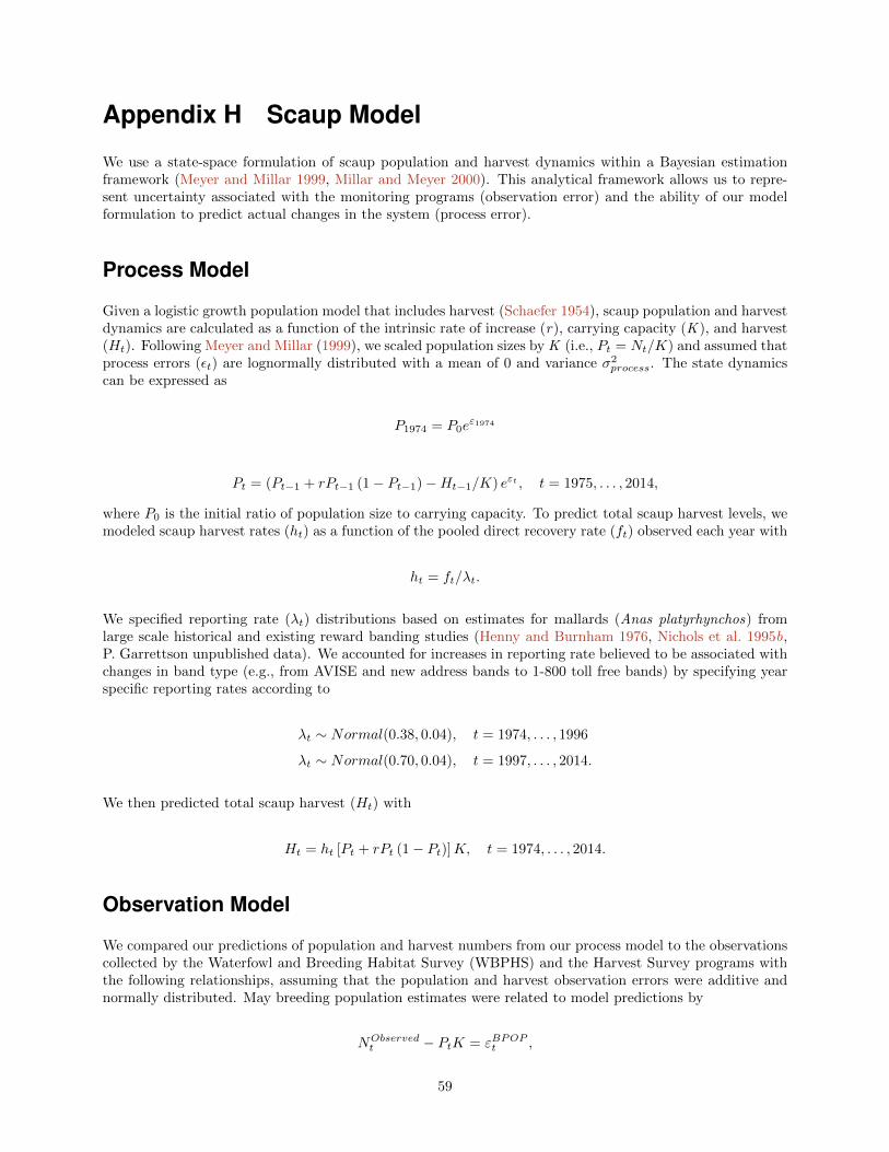
Appendix H Scaup Model

We use a state-space formulation of scaup population and harvest dynamics within a Bayesian estimationframework (Meyer and Millar 1999, Millar and Meyer 2000). This analytical framework allows us to repre-sent uncertainty associated with the monitoring programs (observation error) and the ability of our modelformulation to predict actual changes in the system (process error).

Process Model

Given a logistic growth population model that includes harvest (Schaefer 1954), scaup population and harvestdynamics are calculated as a function of the intrinsic rate of increase (r), carrying capacity (K ), and harvest(𝐻𝑡). Following Meyer and Millar (1999), we scaled population sizes by K (i.e., 𝑃𝑡 = 𝑁𝑡/𝐾) and assumed thatprocess errors (𝜖𝑡) are lognormally distributed with a mean of 0 and variance 𝜎2

𝑝𝑟𝑜𝑐𝑒𝑠𝑠. The state dynamicscan be expressed as

𝑃1974 = 𝑃0𝑒𝜀1974

𝑃𝑡 = (𝑃𝑡−1 + 𝑟𝑃𝑡−1 (1− 𝑃𝑡−1)−𝐻𝑡−1/𝐾) 𝑒𝜀𝑡 , 𝑡 = 1975, . . . , 2014,

where 𝑃0 is the initial ratio of population size to carrying capacity. To predict total scaup harvest levels, wemodeled scaup harvest rates (ℎ𝑡) as a function of the pooled direct recovery rate (𝑓𝑡) observed each year with

ℎ𝑡 = 𝑓𝑡/𝜆𝑡.

We specified reporting rate (𝜆𝑡) distributions based on estimates for mallards (Anas platyrhynchos) fromlarge scale historical and existing reward banding studies (Henny and Burnham 1976, Nichols et al. 1995b,P. Garrettson unpublished data). We accounted for increases in reporting rate believed to be associated withchanges in band type (e.g., from AVISE and new address bands to 1-800 toll free bands) by specifying yearspecific reporting rates according to

𝜆𝑡 ∼ 𝑁𝑜𝑟𝑚𝑎𝑙(0.38, 0.04), 𝑡 = 1974, . . . , 1996

𝜆𝑡 ∼ 𝑁𝑜𝑟𝑚𝑎𝑙(0.70, 0.04), 𝑡 = 1997, . . . , 2014.

We then predicted total scaup harvest (𝐻𝑡) with

𝐻𝑡 = ℎ𝑡 [𝑃𝑡 + 𝑟𝑃𝑡 (1− 𝑃𝑡)]𝐾, 𝑡 = 1974, . . . , 2014.

Observation Model

We compared our predictions of population and harvest numbers from our process model to the observationscollected by the Waterfowl and Breeding Habitat Survey (WBPHS) and the Harvest Survey programs withthe following relationships, assuming that the population and harvest observation errors were additive andnormally distributed. May breeding population estimates were related to model predictions by

𝑁𝑂𝑏𝑠𝑒𝑟𝑣𝑒𝑑𝑡 − 𝑃𝑡𝐾 = 𝜀𝐵𝑃𝑂𝑃

𝑡 ,

59

where

𝜀𝐵𝑃𝑂𝑃𝑡 ∼ 𝑁(0, 𝜎2

𝑡,𝐵𝑃𝑂𝑃 ), 𝑡 = 1974, . . . , 2014,

where 𝜎2𝑡,𝐵𝑃𝑂𝑃 is specified each year with the BPOP variance estimates from the WBPHS.

We adjusted our harvest predictions to the observed harvest data estimates with a scaling parameter (q)according to

𝐻𝑂𝑏𝑠𝑒𝑟𝑣𝑒𝑑𝑡 − (ℎ𝑡 [𝑃𝑡 + 𝑟𝑃𝑡 (1− 𝑃𝑡)]𝐾) /𝑞 = 𝜀𝐻𝑡 , 𝑡 = 1974, . . . , 2014,

where,

𝜀𝐻𝑡 ∼ 𝑁(0, 𝜎2𝑡,𝐻𝑎𝑟𝑣𝑒𝑠𝑡).

We assumed that appropriate measures of the harvest observation error 𝜎2𝑡,𝐻𝑎𝑟𝑣𝑒𝑠𝑡 could be approximated by

assuming a coefficient of variation for each annual harvest estimate equal to 0.15 (Paul Padding pers. comm.).The final component of the likelihood included the year specific direct recovery rates that were representedby the rate parameter (𝑓𝑡) of a Binomial distribution indexed by the total number of birds banded preseasonand estimated with,

𝑓𝑡 = 𝑚𝑡/𝑀𝑡,

𝑚𝑡 ∼ 𝐵𝑖𝑛𝑜𝑚𝑖𝑎𝑙(𝑀𝑡, 𝑓𝑡)

where 𝑚𝑡 is the total number of scaup banded preseason in year t and recovered during the hunting seasonin year t and 𝑀𝑡 is the total number of scaup banded preseason in year t.

Bayesian Analysis

Following Meyer and Millar (1999), we developed a fully conditional joint probability model, by first proposingprior distributions for all model parameters and unobserved system states and secondly by developing a fullyconditional likelihood for each sampling distribution.

Prior Distributions

For this analysis, a joint prior distribution is required because the unknown system states P are assumed tobe conditionally independent (Meyer and Millar 1999). This leads to the following joint prior distribution forthe model parameters and unobserved system states

𝑃 (𝑟,𝐾, 𝑞, 𝑓𝑡, 𝜆𝑡, 𝜎2𝑃𝑟𝑜𝑐𝑒𝑠𝑠, 𝑃0, 𝑃1,...,𝑇 ) =

𝑝(𝑟)𝑝(𝐾)𝑝(𝑞)𝑝(𝑓𝑡)𝑝(𝜆𝑡)𝑝(𝜎2𝑃𝑟𝑜𝑐𝑒𝑠𝑠)𝑝(𝑃0)𝑝(𝑃1|𝑃0, 𝜎

2𝑃𝑟𝑜𝑐𝑒𝑠𝑠)

×𝑛∏

𝑡=2

𝑝(𝑃𝑡|𝑃𝑡−1, 𝑟,𝐾, 𝑓𝑡−1, 𝜆𝑡−1, 𝜎2𝑃𝑟𝑜𝑐𝑒𝑠𝑠)

In general, we chose non-informative priors to represent the uncertainty we have in specifying the value ofthe parameters used in our assessment. However, we were required to use existing information to specify

60

informative priors for the initial ratio of population size to carrying capacity (𝑃0) as well as the reportingrate values (𝜆𝑡) specified above that were used to adjust the direct recovery rate estimates to harvest rates.

We specified that the value of 𝑃0, ranged from the population size at maximum sustained yield (𝑃0 =𝑁𝑀𝑆𝑌 /𝐾 = (𝐾/2)/𝐾 = 0.5) to the carrying capacity (𝑃0 = 𝑁/𝐾 = 1), using a uniform distribution on thelog scale to represent this range of values. We assumed that the exploitation experienced at this populationstate was somewhere on the right-hand shoulder of a sustained yield curve (i.e., between MSY and K ). Giventhat we have very little evidence to suggest that historical scaup harvest levels were limiting scaup populationgrowth, this seems like a reasonable prior distribution.

We used non-informative prior distributions to represent the variance and scaling terms, while the priors forthe population parameters r and K were chosen to be vague but within biological bounds. These distributionswere specified according to

𝑃0 ∼ 𝑈𝑛𝑖𝑓𝑜𝑟𝑚(𝑙𝑛(0.5), 0),

𝐾 ∼ 𝐿𝑜𝑔𝑛𝑜𝑟𝑚𝑎𝑙(2.17, 0.667),

𝑟 ∼ 𝑈𝑛𝑖𝑓𝑜𝑟𝑚(0.00001, 2),

𝑓𝑡 ∼ 𝐵𝑒𝑡𝑎(0.5, 0.5),

𝑞 ∼ 𝑈𝑛𝑖𝑓𝑜𝑟𝑚(0.0, 2),

𝜎2𝑃𝑟𝑜𝑐𝑒𝑠𝑠 ∼ 𝐼𝑛𝑣𝑒𝑟𝑠𝑒 𝐺𝑎𝑚𝑚𝑎(0.001, 0.001).

Likelihood

We related the observed population, total harvest estimates, and observed direct recoveries to the modelparameters and unobserved system states with the following likelihood function:

𝑃 (𝑁1,...,𝑇 , 𝐻1,...,𝑇 ,𝑚1,...,𝑇𝑀1,...,𝑇 |𝑟,𝐾, 𝑓𝑡, 𝜆𝑡, 𝑞, 𝜎2𝑃𝑟𝑜𝑐𝑒𝑠𝑠, 𝜎

2𝐻𝑎𝑟𝑣𝑒𝑠𝑡, 𝑃1,...,𝑇 ) =

×𝑇∏

𝑡=1

𝑝(𝑁𝑡|𝑃𝑡,𝐾, 𝜎2𝐵𝑃𝑂𝑃 )×

𝑇∏𝑡=1

𝑝(𝐻𝑡|𝑃𝑡, 𝑟,𝐾, 𝑞, 𝑓𝑡, 𝜆𝑡, 𝜎2𝐻𝑎𝑟𝑣𝑒𝑠𝑡)

×𝑇∏

𝑡=1

𝑝(𝑚𝑡|𝑀𝑡, 𝑓𝑡)

Posterior Evaluation

Using Bayes theorem we then specified a posterior distribution for the fully conditional joint probabilitydistribution of the parameters given the observed information according to

𝑃 (𝑟,𝐾, 𝑞, 𝑓𝑡, 𝜆𝑡, 𝜎2𝑃𝑟𝑜𝑐𝑒𝑠𝑠, 𝑃0, 𝑃1,...,𝑇 |𝑁1,...,𝑇 , 𝐻1,...,𝑇 ,𝑚1,...,𝑇 ,𝑀1,...,𝑇 ) ∝

𝑝(𝑟)𝑝(𝐾)𝑝(𝑞)𝑝(𝑓𝑡)𝑝(𝜆𝑡)𝑝(𝜎2𝑃𝑟𝑜𝑐𝑒𝑠𝑠)𝑝(𝑃0)𝑝(𝑃1|𝑃0, 𝜎

2𝑃𝑟𝑜𝑐𝑒𝑠𝑠)

×𝑛∏

𝑡=2

𝑝(𝑃𝑡|𝑃𝑡−1, 𝑟,𝐾, 𝑓𝑡−1, 𝜆𝑡−1, 𝜎2𝑃𝑟𝑜𝑐𝑒𝑠𝑠)×

𝑇∏𝑡=1

𝑝(𝑁𝑡|𝑃𝑡,𝐾, 𝜎2𝐵𝑃𝑂𝑃 )

×𝑇∏

𝑡=1

𝑝(𝐻𝑡|𝑃𝑡, 𝑟,𝐾, 𝑞, 𝑓𝑡, 𝜆𝑡, 𝜎2𝐻𝑎𝑟𝑣𝑒𝑠𝑡)×

𝑇∏𝑡=1

𝑝(𝑚𝑡|𝑀𝑡, 𝑓𝑡)

61

Table H.1 – Model parameter estimates resulting from a Bayesian analysis of scaup breeding population, harvest,and banding information from 1974 to 2014.

Parameter Mean SD 2.5% CI Median 97.5% CI

r 0.1464 0.0536 0.0648 0.1387 0.2724

K 8.3649 1.6674 6.0000 8.0410 12.1602

𝜎2 0.0077 0.0033 0.0030 0.0071 0.0157

q 0.6575 0.0384 0.5862 0.6562 0.7365

We used Markov Chain Monte Carlo (MCMC) methods to evaluate the posterior distribution using WinBUGS(Spiegelhalter et al. 2003). We randomly generated initial values and simulated 5 independent chains eachwith 1,000,000 iterations. We discarded the first half of the simulation and thinned each chain by 250, yieldinga sample of 10,000 points. We calculated Gelman-Rubin statistics (Brooks and Gelman 1998) to monitor forlack of convergence. The state space formulation and Bayesian analysis framework provided reasonable fitsto the observed breeding population and total harvest estimates with realistic measures of variation. The2014 posterior estimates of model parameters based on data from 1974 to 2014 are provided in Table H.1.

We further summarized the simulation results for r, K, and the scaling parameter q to admit parametricuncertainty with a formal correlation structure within the optimization procedure used to calculate theharvest strategy. We first defined a joint distribution for 3 discrete outcomes for each of the 3 populationparameters. We used the 30 and 70 percent quantiles for each parameter as the cut points to define threebins for which to discretize 3 values of each posterior distribution. We then determined the frequency ofoccurrence of each of the 27 possible combinations of each parameter value falling within the 3 bins from theMCMC simulation results. These frequencies were then assigned parameter values based on the midpoint ofthe bin ranges (15, 50, 85 percent quantiles) to specify the joint distribution of the population parametervalues used in the optimization.

62

Division of Migratory Bird Management11510 American Holly Dr.Laurel, MD 20708-4016

U.S. Fish & Wildlife Servicehttp://www.fws.gov

For state transfer relay serviceTTY/Voice: 711