Embed Size (px)
Citation preview
ADAPTATION PLANNING UNDER CLIMATE CHANGE
UNCERTAINTY
Using Multi-Criteria Robust Decision Analysis in a Water Resource
System
Lan Ngoc Hoang
Submitted in accordance with the requirements for the degree of
DPhil in Environmental Science
The University of Leeds
School of Earth and Environment
Sustainability Research Institute
July 2013
- ii -
The candidate confirms that the work submitted is her own and that appropriate
credit has been given where reference has been made to the work of others.
This copy has been supplied on the understanding that it is copyright material and
that no quotation from the thesis may be published without proper
acknowledgement.
The right of Lan Ngoc Hoang to be identified as Author of this work has been
asserted by her in accordance with the Copyright, Designs and Patents Act 1988.
© 2013 The University of Leeds and Lan Ngoc Hoang
- iii -
I would like to express my sincere gratitude to my supervisors Professor Suraje Dessai and
Professor Nigel Wright for the continuous support of my Ph.D study and research, for their
patience, motivation, enthusiasm, and immense knowledge. Their guidance helped me in all
the time of research and writing of this thesis. I would also like to thank Associate Professor
Richard Brazier for his continued advice. The good advice and support of the ARCC-
WATER project members has been invaluable to me, for which I am extremely thankful. I
am most grateful to Dr Steven Wade at HR Wallingford Ltd. and Dr Marek Makowski for
providing me with the basis of my modelling work during my research visit to HR
Wallingford Ltd. and the International Institute of Applied System Analysis. A special
thank to Dr Mike Packman (Southern Water Ltd.), Dr Doug Hunt, Mr Dan Wykeham and
Dr Geoff Darch from Atkins Ltd. for giving me insightful advice, as well as providing the
much needed data and information for my case study.
I would like to acknowledge the financial, academic and technical support of the
Engineering and Physical Sciences Research Council, the ARCC-WATER Project, the
University of Leeds, the University of Exeter and the International Institute of Applied
System Analysis. Other funding for workshop participation from the NCAR Advanced
Study Program, the EQUIP project and the EASY-ECO project is also acknowledged.
I am thankful for and would like to acknowledge many others who helped me along the
way: my parents and my sister Dzung, who proofread this thesis; and my friends and
colleagues at Leeds University and the International Institute of Applied System Analysis
for bouncing ideas and sharing the journey with me. Other thanks go to my friends Steve
Orchard, Tuan Thi, Tuan Anh Tran, Diu Nguyen and Hung Bui for offering casual chit chat
about the research and other irrelevant gossip.
For any errors or inadequacies that may remain in this work, of course, the responsibility is
entirely my own.
Acknowledgements
- iv -
This project explores the uncertainty factors in drought planning for a water resource zone in
Sussex. Nine planning options from the 2009 Sussex Water Resource Management Plan were
assessed using four climate products: the 2009 UK Climate Projections Change Factors, the
Spatial Coherent Projections, the 11 runs of the HadRM3 regional climate model and their
subsequent downscaling by the Future Flows Project. The varying drought statistics from these
four climate products reflect post-processing uncertainty - the uncertainty stemming from the
process of converting original climate model outputs into products of different formats, variables
and temporal/spatial scales. Overall, the study has integrated a cascade analysis of climate
uncertainty, climate post-processing uncertainty, hydrological uncertainty, water resource model
uncertainty and demand uncertainty on water resource planning. The study combines Robust
Optimisation, Decision-Scaling and Robust Decision Making into Robust Decision Analysis, a
decision making framework for dynamic adaptation pathways in response to different levels of
uncertainty and risk averseness. Post-processing uncertainty is the dominate uncertainty until
2030s; 2050s is then dominated by demand and socio-economic uncertainty. The most severe
droughts within the Spatial Coherent Projections and the 2009 UK Climate Projection products
are variations of the 1975-1976 and the 1988-1989 droughts, two of the worst historic droughts
currently used as the design events for drought planning in Sussex. The system appears to be
robust to variations of these past droughts. Yet, under different sequences of droughts from the
HadRM3 and Future Flows products, the system demonstrated frequent supply failures in the
2050s, unless water demand is maintained at the 2007 level or lower. While operational costs in
the 2030s are generally within the region of 4 to 5 million GBP per year, those in the 2050s
Market Forces jumped to the region of 5 to 15 million GBP per year and with supply deficit
from 0 to 1100 Ml/year. When demand grows by 35% from the 2007 baseline level, universal
metering becomes a key option. Despite climate post-processing uncertainty, the main hotspots
of water deficits remains similar across the climate products and are driven by network bottle-
necks and the continually high dependence of the system on water sources around the Hardham
area. The study also indicates that inter-regional transfers might not be as reliable as assumed.
Keywords: water resource planning, robust decision analysis, multi-criteria, adaptation, climate
products
Abstract
- v -
Acknowledgements ................................................................................................... iii
Abstract ..................................................................................................................... iv
Table of Contents ...................................................................................................... v
List of Tables ............................................................................................................. x
List of Figures ........................................................................................................... xi
List of Key Abbreviations ..................................................................................... xvii
Chapter 1. INTRODUCTION .......................................................................... 1
1.1. WHAT ARE THE KEY FACTORS TO ADAPTATION SUCCESS? ................................................................................................ 2
1.1.1. Why adapt and what is adaptation success? ............................ 2
1.1.2. Robustness, resilience and vulnerability: why are they relevant to the issue of adaptation .................................................... 4
1.2. RESEARCH QUESTIONS, AIMS AND OBJECTIVES ........................ 6
1.3. THESIS OUTLINE ................................................................................... 7
Chapter 2. LITERATURE REVIEW .............................................................. 9
2.1. INTRODUCTION .................................................................................... 9
2.2. WHY ROBUST WATER RESOURCES SYSTEMS ARE NEEDED IN A CHANGING CLIMATE? ............................................. 10
2.2.1. Water resources planning as a decision analysis problem .......................................................................................... 10
2.2.2. Towards robust water resources system in a changing climate: What is lacking? ............................................................... 12
2.3. UNCERTAINTY MANAGEMENT IN WATER RESOURCES PLANNING AND RELATED FIELD ................................................... 14
2.3.1. Robustness in adaptation decisions ....................................... 14
2.3.2. Robustness in water resources planning ............................... 17
2.3.2.1. Robust optimisation ........................................................ 17
2.3.2.2. Real Options Analysis .................................................... 18
2.3.2.3. Info-gap decision theory ................................................. 20
2.3.2.4. Robust Decision Making ................................................ 22
2.4. ROBUST DECISION ANALYSIS IN A COMPLEMENTARY FRAMEWORK ....................................................................................... 25
2.4.1. Adaptation decision: option robustness and system robustness ....................................................................................... 25
Table of Contents
- vi -
2.4.2. Comparison of methodologies .............................................. 26
2.4.3. A framework linking the robustness concepts ...................... 28
Chapter 3. METHODOLOGY ....................................................................... 33
3.1. LINKING AND INTEGRATING UNCERTAINTY ............................. 33
3.1.1. ‘Top-down’ and ‘bottom-up’ approaches ............................. 33
3.1.2. Bridging approaches: the challenge ...................................... 37
3.2. THE ROBUST DECISION ANALYSIS FRAMEWORK ..................... 39
3.2.1. Aims and objectives .............................................................. 39
3.2.2. Structure ................................................................................ 41
3.2.3. Data structure ........................................................................ 45
3.3. CONCLUSION ....................................................................................... 48
Chapter 4. CASE STUDY DESCRIPTION .................................................. 50
4.1. WATER RESOURCE MANAGEMENT IN ENGLAND AND WALES ................................................................................................... 50
4.1.1. A brief description ................................................................. 50
4.1.2. Planning decision cycles and decision variables ................... 54
4.1.3. Drought planning approaches ................................................ 58
4.2. THE CASE STUDY AREA .................................................................... 60
4.2.1. Water resources and water management of Sussex .............. 60
4.2.2. Main requirements of adaptation: perspectives of the decision makers .............................................................................. 65
4.3. APPLICATION OF THE FRAMEWORK ............................................. 67
4.3.1. Climate uncertainty ............................................................... 67
4.3.2. Hydrological data and model ................................................ 69
4.3.3. Demand modelling ................................................................ 69
4.3.4. Water resource modelling and option analysis ..................... 70
4.3.5. Robust decision analysis ....................................................... 71
4.4. CONCLUSION ....................................................................................... 72
Chapter 5. CLIMATE UNCERTAINTY ...................................................... 74
5.1. INTRODUCTION ................................................................................... 74
5.2. METHODOLOGY .................................................................................. 77
5.2.1. Emission scenarios and climate projections .......................... 77
5.2.2. Drought Indices ..................................................................... 83
5.2.2.1. A brief review of drought indices ................................... 83
5.2.2.2. The Standardised Precipitation Index ............................. 85
- vii -
5.2.2.3. The Standardised Precipitation Evapotranspiration Index ...................................................................................... 86
5.2.3. Data and methods .................................................................. 88
5.2.4. Historic data .......................................................................... 89
5.2.5. Potential evapotranspiration calculation ............................... 90
5.3. RESULTS AND DISCUSSION ............................................................. 92
5.3.1. Potential Evapotranspiration ................................................. 92
5.3.2. Analysis of the climate products ........................................... 95
5.3.2.1. Comparison with observations ....................................... 95
5.3.2.2. UKCP09 and SCP: spatial coherence of climate data97
5.3.2.3. SPI versus SPEI: a comparison of the two indices ....... 101
5.3.2.4. SPI and SPEI-based drought frequency analysis .......... 105
5.4. CONCLUSIONS ................................................................................... 113
Chapter 6. HYDROLOGICAL UNCERTAINTY ..................................... 115
6.1. INTRODUCTION ................................................................................ 115
6.2. METHODOLOGY ................................................................................ 117
6.2.1. The CATCHMOD hydrologic model ................................. 117
6.2.2. The GLUE methodology and Sobol sensitivity analysis .... 120
6.2.2.1. The GLUE methodology .............................................. 121
6.2.2.2. Sobol Sensitivity Analysis ............................................ 123
6.2.2.3. Input data ...................................................................... 124
6.2.2.4. Experimental design ..................................................... 127
6.2.2.5. The efficiency criteria................................................... 128
6.3. RESULTS AND DISCUSSION ........................................................... 128
6.3.1. The effect of soil storage on flows: Comparison of observation and SPEI ................................................................... 128
6.3.2. The ranging low flows of the ‘behavioural’ group ............. 130
6.3.1. Sobol analysis of parameter influences ............................... 139
6.3.1.1. 1959-2004 historic flow analysis.................................. 139
6.3.1.2. Low flow indicators: .................................................... 140
6.3.1.3. Nash value .................................................................... 142
6.3.1.4. The influence of the initial conditions .......................... 145
6.3.2. Future Flows analysis on parameter influences .................. 145
6.3.2.1. Low flows ..................................................................... 145
6.3.2.2. High flows .................................................................... 147
- viii -
6.4. CONCLUSION ..................................................................................... 148
Chapter 7. VULNERABILITY ANALYSIS USING WATER RESOURCE MODELS ............................................................................... 150
7.1. INTRODUCTION ................................................................................. 150
7.2. METHODOLOGY ................................................................................ 152
7.2.1. The scenarios ....................................................................... 152
7.2.2. Climate scenarios ................................................................ 153
7.2.3. Socio-economic scenarios ................................................... 153
7.2.4. Water resource models ........................................................ 159
7.2.4.1. The reference model ..................................................... 159
7.2.4.2. The VB.NET Simulation Model ................................... 160
7.2.4.3. The GAMS Optimisation Model .................................. 161
7.2.4.4. Comparison of the three models ................................... 163
7.3. RESULTS AND DISCUSSION ........................................................... 165
7.3.1. Comparison of the simulation and the optimisation model against the reference model ............................................... 165
7.3.2. Simulation model results ..................................................... 170
7.3.3. Optimisation Model Results ................................................ 173
7.3.4. Vulnerable areas .................................................................. 175
7.3.5. Most severe droughts in each climate product .................... 179
7.4. CONCLUSION ..................................................................................... 181
Chapter 8. WATER RESOURCE PLANNING UNDER UNCERTAINTY .......................................................................................... 183
8.1. INTRODUCTION ................................................................................. 183
8.2. METHODOLOGY ................................................................................ 186
8.2.1. Problem formulation ........................................................... 186
8.2.2. Core model specification ..................................................... 186
8.2.3. Strategy representation ........................................................ 187
8.2.4. Criteria ................................................................................. 192
8.2.5. Scenarios ............................................................................. 193
8.2.6. Robust Decision Analysis using the Simulation Model ...... 193
8.3. RESULTS AND DISCUSSION ........................................................... 194
8.3.1. Option Selection .................................................................. 194
8.3.2. Deficit Analysis ................................................................... 214
8.3.3. Robust Options Analysis ..................................................... 219
8.4. CONCLUSION ..................................................................................... 227
- ix -
Chapter 9. ROBUST ADAPTATION PATHWAY ANALYSIS- A DISCUSSION ............................................................................................... 230
9.1. REVISITING ROBUSTNESS IN THE SUSSEX CONTEXT ............ 230
9.1.1. Comparison of the robustness frameworks ......................... 230
9.1.2. Adaptation Robustness Analysis ......................................... 232
9.1.2.1. Robustness to climate uncertainty and water resource uncertainty ............................................................ 232
9.1.2.2. Robustness to inflow changes ...................................... 235
9.1.2.3. Robustness to Demand Changes .................................. 241
9.1.2.4. Robustness to different supply reliability ..................... 243
9.1.2.5. Robustness to adaptation plan switching ...................... 245
9.2. FACTORS TO ADAPTATION SUCCESS- A WIDER CONTEXT ............................................................................................ 250
Chapter 10. CONCLUSIONS AND RECOMMENDATIONS FOR RESEARCH ................................................................................................. 254
10.1. REVIEW OF RESEARCH AIMS AND SUPPORTING FINDINGS ............................................................................................ 254
10.1.1. Review different definitions and approaches of the concept of robustness in water resource planning: ...................... 254
10.1.2. Conduct a case study in south-east England that incorporates the main aspects of the robustness concept: ............ 255
10.1.3. Use robust decision making to demonstrate how the uncertainty components could affect the performance of adaptation options: ....................................................................... 257
10.1.4. Key findings ........................................................................ 258
10.1.5. Limitations .......................................................................... 259
10.2. IMPLICATIONS FOR ADAPTATION POLICY AND PRACTICE ........................................................................................... 260
10.3. RECOMMENDATION FOR FURTHER RESEARCH ...................... 262
List of References .................................................................................................. 263
Appendix A-Model Descriptions .......................................................................... 279
Appendix B-Model Parameters ........................................................................... 287
Appendix C-The worst droughts according to each climate product in Brighton and Worthing ............................................................................... 289
Glossary .................................................................................................................. 291
- x -
Table 1-1 Definitions of adaptation characteristics in Adger et al. (2005), Smit et al. (2000) ................................................................................................ 3
Table 2-1 Comparative analysis of robustness measure and approaches (the classical robustness refers to Hashimoto et al., 1982) ..................................... 27
Table 4-1 Descriptions of drought permits and drought orders. Modified from: Department of Environment (2011) ................................................................. 53
Table 4-2 Sources of uncertainty for headroom calculation. .................................... 58
Table 4-3 Extracted survey results on managers’ perceptions of global warming scenarios by Subak (2000) ................................................................ 59
Table 5-1 Summary of the climate products used in the study ................................. 81
Table 5-2 Characteristics of some drought indices. Source: Byun and Wilhite (1999) ............................................................................................................... 85
Table 5-3 Classification of droughts according to SPI values. Source: McKee et al. (1993) ...................................................................................................... 86
Table 5-4 Summary of available historic data .......................................................... 89
Table 6-1 CATCHMOD parameters and the sampling range ................................. 125
Table 6-2 Original CATCHMOD parameters and contributing zone characterisation .............................................................................................. 126
Table 6-3 Sobol sensitivity indices of the 10 most influential parameters or interactions on the corresponding criteria. ..................................................... 139
Table 6-4 Sobol sensitivity indices of the 10 most influential CATCHMOD parameters or interactions on the low flow of the FF climate product. ......... 146
Table 6-5 Sobol sensitivity indices of the 10 most influential CATCHMOD parameters or interactions on the high flows of the FF climate product. ....... 147
Table 7-1 Supply cost of source nodes in the Sussex Optimisation Model ............ 162
Table 7-2 Comparison of the three water resource models ..................................... 164
Table 7-3 Contributing factors to the reduction and increase of supply deficit in each model ................................................................................................. 169
Table 7-4 Sussex drought year-Optimisation Model .............................................. 180
Table 7-5 Sussex drought year-Simulation Model .................................................. 180
Table 8-1 List of single options selected from Southern Water’s 2009 Water Resource Management Plan (Southern Water, 2009b) and used in the Optimisation Model ....................................................................................... 189
Table 8-2 Unique combinations of the options. 0 denotes not selecting any option. ............................................................................................................. 197
Table 9-1 Potential impact of climate change on groundwater by 2025. ................ 244
List of Tables
- xi -
Figure 2.1 Real Option of managed flood probability with time. ............................. 19
Figure 2.2 Robustness and Opportuneness Curve (Ben-Haim) and robustness curve of a case study of levee raise (Hine and Hall, 2010). ............................. 22
Figure 2.3 Steps in a robust decision making analysis.............................................. 23
Figure 2.4 Framework of adaptive strategy as implemented iteratively in the model. ............................................................................................................... 24
Figure 2.5 Analysis of scenarios, in which the open diamond ones are vulnerable circumstances (Lempert and Groves, 2010) .................................. 25
Figure 2.6 Information representation based on level of confidence ........................ 29
Figure 2.7 Map of methodologies along the uncertainty axis of modelling inputs ................................................................................................................ 29
Figure 2.8 Framework for selecting a robust decision method ................................. 30
Figure 3.1 Comparative diagrams of traditional ‘top-down’ and two ‘bottom-up’ approaches- adapted and combined from Brown et al. (2011) and Lempert and Groves (2010) ............................................................................. 35
Figure 3.2 Factors influencing water transition pathways. Adapted from Foxon et al. (2010) ...................................................................................................... 36
Figure 3.3 The uncertainty cascade (Wilby and Dessai, 2010)................................. 38
Figure 3.4 Proposed Robust Decision Analysis framework ..................................... 42
Figure 3.5 Schematic of the framework .................................................................... 47
Figure 3.6 Schematic of how the adaptation pathway is constructed based on modelling results .............................................................................................. 48
Figure 4.1 Water management framework in England and Wales ........................... 54
Figure 4.2 Schematic of a capacity-expansion problem. Source:Luss (1982) .......... 56
Figure 4.3 The relationship between headroom, demand and supply in the supply demand balance (Environment Agency, 2012). ................................... 57
Figure 4.4 Map of the study area. ............................................................................. 61
Figure 4.5 Geological map of the study area. ........................................................... 62
Figure 4.6 Groundwater abstraction map of the study area. Source: British Geological Survey ............................................................................................ 63
Figure 4.7 Map of metered and un-metered area in the study area ........................... 64
Figure 4.8 Example of UKCP09 and Future Flow data resolution. .......................... 68
Figure 4.9 Uncertainty factors in the study ............................................................... 72
List of Figures
- xii -
Figure 5.1 The nesting RCM approach, in which a RCM is nested in a GCM to provide climate projections of higher spatial resolution. Source: Giorgi (2008) .................................................................................................... 78
Figure 5.2 Schematic of how the climate products are related ................................. 82
Figure 5.3 Time periods of interest in the study ....................................................... 83
Figure 5.4 L-moment ratio diagram for the 1961-1990 baseline of Observed, RCM and FF time series of monthly data. ....................................................... 88
Figure 5.5 Catchments in the study area and available historic dataset .................... 89
Figure 5.6 Comparison of two historic datasets ........................................................ 90
Figure 5.7 Graph of MORECS PET versus FAO-56 Penmann-Monteith PET ........ 92
Figure 5.8 Comparison of temperature-based PET formulae against MORECS PET data ........................................................................................................... 93
Figure 5.9 Comparison of observed rainfall with simulated rainfall from two climate products (RCM and FF) for different time periods (1970s, 1980s and 1990s) for the River Rother catchment. .................................................... 96
Figure 5.10 Standardised Precipitation Index (SPI) for multiple timescales (3, 6, 12 and 24 months) for two climate products (RCM and FF) and observations over the period 1961-1990. ......................................................... 97
Figure 5.11 Comparison of the monthly rainfall change factors of UKCP09 (10,000 blue dots) and SCP (11 red dots) in the grid cell 1704 for the 2020s Mid-Emission climate scenario ............................................................. 98
Figure 5.12 Comparison of precipitation change factors (5) in various SCP grid cells in 2050s ............................................................................................ 99
Figure 5.13 Correlation analysis of monthly rainfall received by the Rother catchment and the Weirwood catchment shows a consistent linear trend across time. ..................................................................................................... 100
Figure 5.14 SPI and SPEI values of the 1914-2006 historic period. ....................... 102
Figure 5.15 Average 3-month SPI changes across time periods based on the 1961-1990 baseline ........................................................................................ 104
Figure 5.16 Average 3-month SPEI changes across time periods based on the corresponding 1961-1990 baseline. ............................................................... 105
Figure 5.17 Average annual frequency (in percentage) of SPI-based moderate drought in different time periods (pre-1961, 1961-90, 2020s, 2030s and 2050s) according to different products (Observations, RCM, FF, SCP, UCKP09) for multiple drought durations (3, 6, 9, 12, 24,36) ........................ 107
Figure 5.18 The annual frequency of SPI-based severe drought risks in different time periods according to different data sources ............................. 108
Figure 5.19 The annual frequency of SPI-based extreme drought risks in different time periods according to different data sources ............................. 109
Figure 5.20 Average Frequency of Moderate Droughts according to the SPEI index on different time scale .......................................................................... 109
- xiii -
Figure 5.21 Average Frequency of Severe Droughts according to the SPEI index on different time scale .......................................................................... 110
Figure 5.22 Average Frequency of Extreme Droughts according to the SPEI index on different time scale .......................................................................... 111
Figure 6.1 Schematic of the CATCHMOD model. Source: Wilby (2005) ............. 118
Figure 6.2 Graph of one-month, two-month, three-month and six-month SPEI versus Rother observed monthly flows (1990-2004) from January to December (right axis). ................................................................................... 129
Figure 6.3 The ranging low flows in the behavioural group ................................... 131
Figure 6.4 Graph of Nash coefficient versus log Nash of the Sample 2 ................. 132
Figure 6.5 Changes of Q90, Q95, Q99 and Q99.99 compared to the 1961-1990 period in the FF climate product. ................................................................... 133
Figure 6.6 Changes of Q90, Q95, Q99 and Q99.99 compared to the 1961-1990 period in the RCM climate product ............................................................... 134
Figure 6.7 Box plots showing the changing trend of flow quantiles (Ml/day) from the historic period to 2020s, 2030s, and 2050s as projected by the four climate products. .................................................................................... 137
Figure 6.8 A closer look at the different projections in low flow quantiles with the additional data of the observed 1990-2005 flows for comparison. .......... 138
Figure 6.9 Graph of the standardized Cq versus the lowest total 7-day flows in six contributing zones. ................................................................................... 141
Figure 6.10 Graph of the standardized Cq versus the log Nash value. ................... 142
Figure 6.11 Contour plot of the influence of the interaction of Phi2 and Cq2 on the overall Nash value. .............................................................................. 144
Figure 7.1 Four UK Future Scenarios for 2020s. .................................................... 155
Figure 7.2 The 2030s four EA scenarios. ................................................................ 156
Figure 7.3 The four demand scenarios of the Environment Agency in England and Wales, modified after Environment Agency (2008) ............................... 157
Figure 7.4 Weekly Demand Profile of Sussex water resource system in the 2020s based on 1995 demand data from Southern Water .............................. 158
Figure 7.5 Weekly Demand of the Sussex water resource system from 2007 to 2050s .............................................................................................................. 159
Figure 7.6 Schematic of the Sussex Simulation Model .......................................... 161
Figure 7.7 Schematic of the Sussex Optimisation Model ....................................... 163
Figure 7.8 Simulated Weirwood reservoir state from 1888 to 2005 ....................... 165
Figure 7.9 Comparison plot of Aquator versus the Optimisation model without Weirwood Reservoir Control Curve .............................................................. 166
Figure 7.10 Aquator versus the Optimisation Model with an all-time implementation of the control curve .............................................................. 167
Figure 7.11 Comparison of the stated Aquator AMP4 control curve versus the actual minimum reservoir state in the run ...................................................... 168
- xiv -
Figure 7.12 Comparison of Aquator versus the optimisation model if the control curve is only applied during high flows ............................................. 169
Figure 7.13 Average annual supply deficit in Sussex North, Sussex Worthing and Sussex Brighton in the 2020s, 2030s and the 2050s time period according to different climate products. ......................................................... 171
Figure 7.14 (Clockwise from top left) ..................................................................... 173
Figure 7.15 Sussex supply deficit over time periods .............................................. 174
Figure 7.16 Sussex environmental deficits (7.16a) and pumping cost (7.16b) over time periods ............................................................................................ 175
Figure 7.17 Deficit locations in the 2020s .............................................................. 176
Figure 7.18 Deficit locations in the 2030s .............................................................. 176
Figure 7.19 Deficit locations in the 2050s Innovation scenario .............................. 177
Figure 7.20 Deficit locations in the 2050s Market Forces scenario ........................ 178
Figure 7.21 Deficit locations in the 2050s Local Resilience scenario .................... 178
Figure 7.22 Deficit locations in the 2050s Sustainable Behaviour scenario ........... 179
Figure 8.1 Schematic of the Sussex Optimisation Model with available water planning options ............................................................................................. 191
Figure 8.2 Supply deficit without options, in the Base Case scenarios, with headroom Demand (5% increase from the Base Case demand), and with headroom Demand and 5% groundwater reduction due to outages ............... 195
Figure 8.3 Average annual cost of maintain low supply deficits in the water resource system in Sussex .............................................................................. 196
Figure 8.4 Selection frequency graph of the option portfolio in 2020s. ................. 200
Figure 8.5 Frequency of usage of each option overall in 2020s.............................. 201
Figure 8.6 Three-dimensional plot of Environmental Deficit versus Pumping Cost and Supply-Demand Deficit in 2020s for the UKCP09 product ........... 202
Figure 8.7 Frequency graph of the option portfolio in 2030s ................................. 203
Figure 8.8 Overall frequency of usage for the selected option in 2030s ................. 204
Figure 8.9 Comparison of option preference under the climate conditions of the RCM and the FF product for the 2030s .................................................... 205
Figure 8.10 Frequency graph of the option portfolio in 2050s under the Innovation socio-economic scenario .............................................................. 206
Figure 8.11 Option usage frequency under 2050s Innovation ................................ 207
Figure 8.12 Frequency graph of the option portfolio in 2050s under the Market Forces scenario ............................................................................................... 208
Figure 8.13 Option usage frequency under 2050s Market Forces .......................... 209
Figure 8.14 Frequency graph of the option portfolio in 2050s under the Local Resilience scenario ......................................................................................... 209
Figure 8.15 Option usage frequency under 2050s Local Resilience ....................... 210
- xv -
Figure 8.16 Frequency graph of the option portfolio in 2050s under the Sustainable Behaviour scenario ..................................................................... 210
Figure 8.17 Option usage frequency under 2050s Sustainable Behaviour ............. 211
Figure 8.18 3D plot of Environmental Deficit versus Pumping Cost and Supply-Demand Deficit in 2030s for the UKCP09 product .......................... 212
Figure 8.19 3D plot of Environmental Deficit versus Pumping Cost and Supply-Demand Deficit in 2050s Market Forces for the UKCP09 product ........................................................................................................... 213
Figure 8.20 Deficit locations in 2020s .................................................................... 215
Figure 8.21 Deficit locations in 2030s .................................................................... 216
Figure 8.22 Deficit locations in 2050s Innovation .................................................. 216
Figure 8.23 Deficit locations in 2050s Market Forces ............................................ 217
Figure 8.24 Deficit locations in 2050s Local Resilience ........................................ 218
Figure 8.25 Deficit locations in 2050s Sustainable Behaviour ............................... 218
Figure 8.26 Average annual supply deficit in the 2020s. ........................................ 220
Figure 8.27 Average annual supply cost in the 2020s. ........................................... 220
Figure 8.28 Average annual supply deficit in the 2030s. The % Frequency colour gradient shows how often the option was selected in the Optimisation Model, such that the option in red was the dominant option of the Optimisation Model. ............................................................................ 222
Figure 8.29 Average annual supply deficit in the 2050s under the Innovation socio-economic scenario ................................................................................ 223
Figure 8.30 Average annual supply deficit in the 2050s under the Sustainable Behaviour socio-economic scenario. The % Frequency colour gradient shows how often the option was selected in the Optimisation Model, such that the option in red was the dominant option of the Optimisation Model. ............................................................................................................ 223
Figure 8.31 Average annual supply deficit in the 2050s under the Local Resilience socio-economic scenario. ............................................................. 224
Figure 8.32 Average annual supply deficit in the 2050s under the Market Forces socio-economic scenario. ................................................................... 226
Figure 8.33 Average annual supply cost in the 2050s under the Market Forces socio-economic scenario. ............................................................................... 227
Figure 9.1 Graph of Q90-Operational Cost-Supply Deficit of the Sussex water resource system under different climate products and headroom uncertainty for the 2020s ............................................................................... 238
Figure 9.2 Graph of Q90-Operational Cost-Supply Deficit of the Sussex water resource system under UKCP09 for the 2020s, 2030s and 2050s Market Forces ............................................................................................................. 240
Figure 9.3 Graph of the changing overall average annual supply deficit as water demand deviates from the 2007 level................................................... 242

- xvi -
Figure 9.4 The ranging performance of each portfolio under different level of alpha ............................................................................................................... 243
Figure 9.5 The most robust adaptation pathways to cope with drought risks projected by FF .............................................................................................. 248
Figure 9.6 Available adaptation pathways to maintain water supply-demand deficit to under 150 Ml/year in all scenarios. ................................................. 249
- xvii -
AMP Asset Management Plan
ASR Aquifer Storage Recharge
AQUASIM Aqua Simulation Model
CAPEX One-off capital investment cost
CATCHMOD Catchment Model
CC Consumer Council
CCDEW The Climate Change and Demand for Water
CEH Centre for Ecology and Hydrology
DEFRA The Department for Environment, Food and Rural
Affairs
Dos Deployable Outputs
DP The Direct Percolation
EA The Environment Agency for England and Wales
FF
FAO
Future Flow
Food and Agriculture Organisation
FRS Family Resource Survey
GAMS Generalised Algebraic Modelling Software
GCMs Global Climate Models
GLUE The Generalised Likelihood Uncertainty Estimation
GW Groundwater
HadRM3 Hadley Centre Regional Climate Model
I Innovation
IPCC The Intergovernmental Panel for Climate Change
IRAS Interactive River-Aquifer Simulation
List of Key Abbreviations

- xviii -
LP/DP Linear or Dynamic programming
LR Local Resilience
MF Market Forces
MOREC The Meteorological Office Rainfall and Evaporation
Calculation system
MOSES The Meteorological Office Surface Exchange Scheme
MRF Minimum Residual Flow
MRFWW Weirwood Minimal Residual Flow
MRSE The Mean Squared Residual of Errors
MSE The Mean Squared Errors
NPV Net Present Value
OFWAT The Water Services Regulation Authority
OPEX Operational cost
PCC Per Capita Consumption
PDSI Palmer Drought Severity Index
PET
PPE
Potential Evapotranspiration
Perturbed Physics Ensembles
Q90 The 90th percentile of daily flows
RCM Regional Climate Model
RDM Robust Decision Making
SAI Standardised Anomaly Index
SB Sustainable Behaviour
SCPs
SDB
The Spatially Coherent Projections
Supply Demand Balance
SEW South East Water
SPEI The Standardised Precipitation- Evapotranspiration
Index
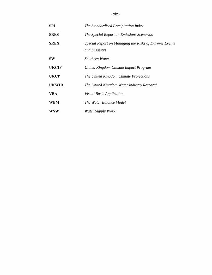
- xix -
SPI The Standardised Precipitation Index
SRES The Special Report on Emissions Scenarios
SREX Special Report on Managing the Risks of Extreme Events
and Disasters
SW Southern Water
UKCIP United Kingdom Climate Impact Program
UKCP The United Kingdom Climate Projections
UKWIR The United Kingdom Water Industry Research
VBA Visual Basic Application
WBM The Water Balance Model
WSW Water Supply Work

Page 1
Chapter 1. INTRODUCTION
Climate change and its subsequent impacts on water resources can affect many
aspects of society and the environment. This is not new. Many early human
civilisations started and revolved around rivers such as the Nile, the Tigris-
Euphrates, the Indus and the Yellow River; many more flourished or failed due to
their capacity to manage and share these water resources (Sadoff and Grey, 2002).
The potential changes in water availability have become a problem for water
management and decision making across both spatial and temporal scales.
Adaptation has become one of the major strategies to cope with climate change.
While adapting to natural changes has been an integral part of the human activities,
the advent of climate change and its impacts can potentially require unprecedented
and widespread adjustments. The last three decades have witnessed a remarkable but
gradual shift in our attitude to the risks of climate change and their subsequent
impacts. Back in 1977, the US Panel on Water and Climate (1977) asserted only a
“small probability of a change in regional climate so abrupt, widespread, severe,
and statistically unambiguous that current water resource design practices need or
should be radically altered...”. Mitigation was viewed as the main response and the
risk was not considered to be pressing for immediate actions. Thirty years later,
numerous studies indicated that we are indeed living in a changing climate (Parry et
al., 2007; Bellard et al., 2012; Doney et al., 2012; Arnell and Gosling, 2013).
Adaptation appears to be an inevitable option due to the level of uncertainty
surrounding the change (Salinger, 2005; Moreira et al., 2007). Hallegatte et al.
(2012) described this level of uncertainty as deep uncertainty, “a situation in which
analysts do not know or cannot agree on (1) models that relate key forces that shape
the future, (2) probability distributions of key variables and parameters in these
models, and/or (3) the value of alternative outcomes” [p.2].
Uncertainty persists from climate projections to subsequent ‘knock-on’ effects on
the ecosystem, the hydrosphere, biosphere and the human societies. In the face of
Page 2
such explosion of uncertainty (Wilby and Dessai), there have been concerns about
the inadequacy of the current water management practices regarding water supply
reliability, flood risk, health, energy and aquatic ecosystems (Kundzewicz et al.,
2008; Minville et al., 2010). The need to move away from the status quo, to adapt
and revisit management policies, as such, is urgent and challenging (Fankhauser et
al., 1999; Adger, 2003; Stern, 2007).
1.1.WHAT ARE THE KEY FACTORS TO ADAPTATION SUCCESS?
1.1.1. Why adapt and what is adaptation success?
Yet, what constitutes adaptation and the factors of adaptation success are still far
from clear. In the context of the water industry, these issues represent major
challenges in current and future planning. Smithers and Smit (1997) have shown
several conceptual foundations of adaptation. Ecological adaptation refers to the
reactive responses and genetic evolution of a species. On the contrary, adaptation in
social sciences emphasises planning and decision making that go beyond species
survival. This study follows the adaptation definition of The Intergovernmental
Panel for Climate Change (IPCC)’s Special Report on Managing the Risks of
Extreme Events and Disasters (SREX), which defines adaptation as adjustments in
human systems to changes in climatic stimuli (Field et al., 2012). Translating these
types of adaptation into the climate change context, adaptation has been classified
into three categories: autonomous (passive and spontaneous adaptation to existing
changes), planned (based on an awareness of historic or near-future changes),
anticipatory (actions before observed impacts of changes) (proactive adaptation)
(McCarthy, 2001). Adaptation can further be described as a process of moving from
sustaining status quo (resilience) to incremental change (transition) and paradigm
shift (transformation) (Pelling, 2011). Smit et al. (2000), meanwhile, characterised
adaptation by the goals (adapt to what?), the actors (who or what adapts) and the
process (how it occurs).
The focus of adaptation is also increasingly placed on enhancing adaptive capacity
instead of specific adaptation measures (Smit and Pilifosova, 2003). Adaptation
Page 3
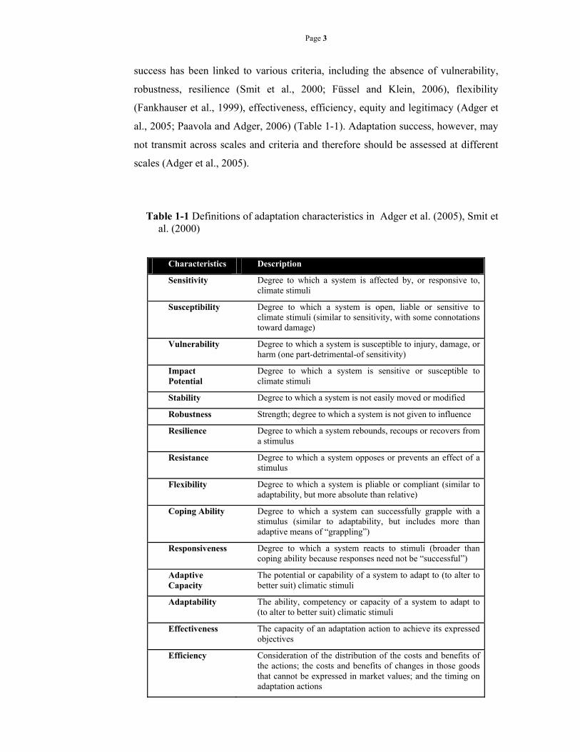
success has been linked to various criteria, including the absence of vulnerability,
robustness, resilience (Smit et al., 2000; Füssel and Klein, 2006), flexibility
(Fankhauser et al., 1999), effectiveness, efficiency, equity and legitimacy (Adger et
al., 2005; Paavola and Adger, 2006) (Table 1-1). Adaptation success, however, may
not transmit across scales and criteria and therefore should be assessed at different
scales (Adger et al., 2005).
Table 1-1 Definitions of adaptation characteristics in Adger et al. (2005), Smit et al. (2000)
Characteristics Description
Sensitivity Degree to which a system is affected by, or responsive to, climate stimuli
Susceptibility Degree to which a system is open, liable or sensitive to climate stimuli (similar to sensitivity, with some connotations toward damage)
Vulnerability Degree to which a system is susceptible to injury, damage, or harm (one part-detrimental-of sensitivity)
Impact Potential
Degree to which a system is sensitive or susceptible to climate stimuli
Stability Degree to which a system is not easily moved or modified
Robustness Strength; degree to which a system is not given to influence
Resilience Degree to which a system rebounds, recoups or recovers from a stimulus
Resistance Degree to which a system opposes or prevents an effect of a stimulus
Flexibility Degree to which a system is pliable or compliant (similar to adaptability, but more absolute than relative)
Coping Ability Degree to which a system can successfully grapple with a stimulus (similar to adaptability, but includes more than adaptive means of “grappling”)
Responsiveness Degree to which a system reacts to stimuli (broader than coping ability because responses need not be “successful”)
Adaptive Capacity
The potential or capability of a system to adapt to (to alter to better suit) climatic stimuli
Adaptability The ability, competency or capacity of a system to adapt to (to alter to better suit) climatic stimuli
Effectiveness The capacity of an adaptation action to achieve its expressed objectives
Efficiency Consideration of the distribution of the costs and benefits of the actions; the costs and benefits of changes in those goods that cannot be expressed in market values; and the timing on adaptation actions
Page 4
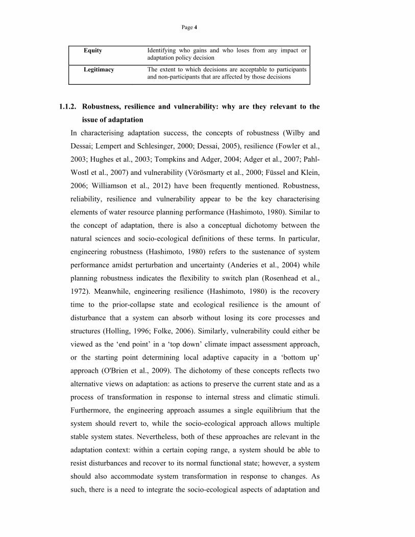
Equity Identifying who gains and who loses from any impact or adaptation policy decision
Legitimacy The extent to which decisions are acceptable to participants and non-participants that are affected by those decisions
1.1.2. Robustness, resilience and vulnerability: why are they relevant to the
issue of adaptation
In characterising adaptation success, the concepts of robustness (Wilby and
Dessai; Lempert and Schlesinger, 2000; Dessai, 2005), resilience (Fowler et al.,
2003; Hughes et al., 2003; Tompkins and Adger, 2004; Adger et al., 2007; Pahl-
Wostl et al., 2007) and vulnerability (Vörösmarty et al., 2000; Füssel and Klein,
2006; Williamson et al., 2012) have been frequently mentioned. Robustness,
reliability, resilience and vulnerability appear to be the key characterising
elements of water resource planning performance (Hashimoto, 1980). Similar to
the concept of adaptation, there is also a conceptual dichotomy between the
natural sciences and socio-ecological definitions of these terms. In particular,
engineering robustness (Hashimoto, 1980) refers to the sustenance of system
performance amidst perturbation and uncertainty (Anderies et al., 2004) while
planning robustness indicates the flexibility to switch plan (Rosenhead et al.,
1972). Meanwhile, engineering resilience (Hashimoto, 1980) is the recovery
time to the prior-collapse state and ecological resilience is the amount of
disturbance that a system can absorb without losing its core processes and
structures (Holling, 1996; Folke, 2006). Similarly, vulnerability could either be
viewed as the ‘end point’ in a ‘top down’ climate impact assessment approach,
or the starting point determining local adaptive capacity in a ‘bottom up’
approach (O'Brien et al., 2009). The dichotomy of these concepts reflects two
alternative views on adaptation: as actions to preserve the current state and as a
process of transformation in response to internal stress and climatic stimuli.
Furthermore, the engineering approach assumes a single equilibrium that the
system should revert to, while the socio-ecological approach allows multiple
stable system states. Nevertheless, both of these approaches are relevant in the
adaptation context: within a certain coping range, a system should be able to
resist disturbances and recover to its normal functional state; however, a system
should also accommodate system transformation in response to changes. As
such, there is a need to integrate the socio-ecological aspects of adaptation and
Page 5
its characteristics into the engineering approach. This study acknowledges both
sides of these concepts and defines the overall robustness as the system capacity
to resist disturbances while maintaining planning flexibility amidst uncertainty.
Resilience is defined as the capacity to regain system functions after disturbance
and vulnerability is the risk of system collapses due to both climatic stimuli and
internal system attributes.
In the face of uncertainty, robustness is a highly relevant concept to adaptation
in water resource planning. The practice of water resource planning has long
relied on the natural water balance and the seasonal cycle of water supply. Yet, a
non-stationary climate requires fundamental revision and renovation of such
practice (Milly et al., 2008). Climate uncertainty appears to be the dominant
uncertainty factor on hydrological response (Arnell, 1999b; Wilby, 2005; Kay et
al., 2009), although the effects are likely to be catchment-dependent (Boorman
and Sefton, 1997).The effects of climate change on water resources are evident
in various catchments and water systems (Leavesley, 1994; Vörösmarty et al.,
2000; Werritty, 2002; Brekke et al., 2004; Wilby et al., 2006; Dessai and Hulme,
2007; Fowler et al., 2007). Water resource systems are sensitive to changes in
both moderate and extreme climate variation (Němec and Schaake, 1982).
Therefore the impacts of these changes on the systems and the decision making
process should be considered.
Nevertheless, integrated studies on how climate uncertainty propagates from the
climate projections to the decision making scale, especially when coupled with
hydrological and socio-economic uncertainty, are sparse. Some examples of
studies within that stream include Dessai and Hulme (2007), Lopez et al.
(2009a), Ranger et al. (2010) , Darch et al. (2011) and Matrosov et al. (2012). To
date, there have been few studies that demonstrate the uncertainty the decision
makers face, in particular with regards to different climate information from
different sources and how selecting the information might affect their decisions.
This issue is vital and relevant to decision making in practice. Furthermore,
water resource planning also needs to consider other stressors such as demand
growth and its associating potential risks. The direct effects of climate change
Page 6
such as the exacerbation of droughts and floods could further interact with
existing demand pressure and lead to other indirect effects of excessive
groundwater abstraction and extra demand pressure (IPCC, 2007). As such, there
is a need for an integrated assessment that includes the relevant uncertainty
factors, analyses their influences on the planning process and identifies potential
robust strategies under such uncertainty.
1.2. RESEARCH QUESTIONS, AIMS AND OBJECTIVES
Further research into how climate uncertainty could affect adaptation decisions
is important and essential. Practitioners such as water managers are currently
incorporating complex climate projections into decision making and need to
consider the role of uncertainty in robust adaptation decisions. Yet climate
projections are subject to deep uncertainties and such uncertainties could cascade
into water resource planning. Furthermore, the overall implications of climate
changes are intertwined with intricate socio-economic changes, leading to even
more uncertain conditions. The research therefore addresses two key questions:
i) How does climate uncertainty in conjunction with impact modelling and
socio-economic uncertainty affect drought planning decisions in water resource
systems?
ii) Can the different criteria to robustness in adaptation decision be integrated
and analysed to inform robust adaptation planning?
The study aims to explore the components in the uncertainty cascade from
climate projections, hydrological modelling, water resource modelling and
option identification. It limits its scope to climate change impacts on surface
water and focuses on the water quantity aspect of drought planning. The
objectives of the research are to:
i) Review different definitions and approaches of the concept of robustness
in water resource planning: different approaches and definitions of robustness
can guide the adaptation decisions towards different goals. This objective
addresses the different underlying ideology of each approach and constructs a
framework that engages the role of each approach.
Page 7
ii) Construct a methodology and water resource models for a case study in
south-east England that incorporates the main aspects of the robustness
concept: The case study serves as an example of how robust adaptation
decisions can be identified in practice. Furthermore it demonstrates how real-life
decision making could incorporate climate change uncertainty along with socio-
economic uncertainty.
iii) Use robust decision making to demonstrate how the uncertainty
components could affect the performance of adaptation options: While being
designed under the robustness framework, adaptation options could still be
susceptible to changes in assumptions and uncertainty bounds. This explores the
varying robustness of adaptation options under different factors and levels of
uncertainty.
1.3.THESIS OUTLINE
Chapter 2 Literature Review reviews the key approaches to robustness and
their associated criteria. It compares and contrasts Robust Optimisation, Real
Option analysis, Info-gap Decision Theory and Robust Decision Making. It also
presents a linking decision framework that emphasises the utility of these
methodologies in reiterative planning cycles.
Chapter 3 Methodology describes the study framework to analyse uncertainty
propagation and potential adaptation pathways that balance vulnerability and
financial costs. It links elements of the uncertainty cascade and combines multi-
criteria analysis with scenario planning to assess the overall impacts of
uncertainty on drought planning options.
Chapter 4 Study Area describes the study area and adaptation context in
details. It highlights the local relevant features to adaptation and outlines the
steps of the subsequent assessments in Chapter 5 to Chapter 8.
Chapter 5 Climate Uncertainty explains the key characteristics of four climate
products: the original Regional Climate Model HadRM3 ensembles, their
downscaled projections produced by the Future Flows project, the UK Climate
Program Spatial Coherent Projections (SCP) and the 2009 UK Climate
Page 8
Projections (UKCP09) full set of 10,000 realisations. It analyses two uncertainty
factors: the climate uncertainty represented by each of these products, and the
uncertainty from the post-processing procedure that produces these products.
Chapter 6 Hydrological Uncertainty compares the climate uncertainty with the
Generalised Likelihood Uncertainty Estimation (GLUE) of hydrological
uncertainty. The chapter also employs Sobol-sensitivity analysis to explore
parameter interaction under different flow conditions.
Chapter 7 Vulnerability Analysis examines the capacity of the current water
resource system to cope with projected future changes in the 2020s, 2030s and
2050s. Considered uncertainty factors include climate uncertainty, post-
processing uncertainty and socio-economic uncertainty. The chapter uses a
simulation model and an optimisation model to produce vulnerability results as
well as identify the severe drought years in each climate product.
Chapter 8 Option Analysis continues to assess the coping capacity of the
system and potential options under deep uncertainty. The Chapter uses the
Optimisation Model to identify packages of robust measures and the Simulation
Model to test their performance under all planning scenarios. It also explores the
cascaded uncertainty from the climate component and the different impacts
projections due to using different climate products.
Chapter 9 Robust Adaptation Pathway Discussion revisits the aspects of
robustness discussed in Chapter 2 and connects the findings with that theoretical
framework. It analyses the robustness of the case study system to climate
uncertainty, post-processing uncertainty, changing inflows, varying supply
reliability and alternative socio-economic scenarios. It also assesses the system
under the lens of planning robustness and plan switches. Finally it examines the
assumptions and social uncertainty that could not be included in the modelling
process.
Chapter 10 Conclusion summarises the all findings in views of the objectives
laid out at the onset of the thesis. It reviews remaining limitations and presents
recommendations for further research.
Page 9
2.1.INTRODUCTION
A certain amount of climate change is now unavoidable and requires timely
adaptation decisions in water resource planning. Yet, projections of local climate
change impacts are plagued with substantial unknowns, which make anticipatory
adaptation difficult. As the climate is shifting, so are stream flows, occurrence of
extreme events, and subsequently, the practice of water modelling and management
(Arnell et al., 2001; Milly et al., 2008; Hirschboeck, 2009; Lins and Cohn, 2011;
Peel and Blöschl, 2011). While non-stationarity in the climate and particularly the
hydrological cycle is not essentially a new issue, climate change impacts emphasise
the need to reconsider and incorporate principles of risk aversion and adaptation into
water resources systems (Lins and Cohn, 2011). The risk introduced by climate
change impacts has a wide range and high level of uncertainty, which frequently
prompts the term “deep uncertainty” (Lempert and Groves, 2010). By definition,
uncertainty is imprecise knowledge about the probability, distribution of events and
the magnitude of their consequences on vulnerable receptors (Knight, 1921). Deep
uncertainty, a subcategory, lies at the fuzzier end of uncertainty, where the direction
and magnitude of changes are completely unknown (Bammer and Smithson, 2008).
The capacity to maintain performance amidst uncertainty (also known as robustness)
(Lempert and Schlesinger, 2000; Dessai, 2005) and the ability to absorb such
disturbance (resilience) (Janssen and Anderies, 2007; Ben-Tal et al., 2009) has thus
been increasingly used to assess water-resource systems.
Despite its analytical importance, robustness and its attributes have not been
consistently defined in the literature of water resource planning. This ambiguity in
terminology has been noticed in various documents concerning climate change
impacts. For instance, in response to the 2006 draft report on climate decision
making by the US Climate Change Science Program (Bertsimas et al., 2010), the
Chapter 2. LITERATURE REVIEW
Page 10
review committee of the US National Research Council found the concept of
robustness “insufficiently defined” (Ben-Tal and Nemirovski, 2002). Similarly, the
Water Resources Planning Guideline by the Environment Agency for England and
Wales (Environment Agency, 2012) stated robustness as a key requirement, yet,
without any formal definition of the term.
The various definitions of “robustness” in current water resources planning can
often be traced back to operational research, managerial science, statistics and
control theory. These alternative paradigms underline various aspects and
underlying philosophies which may or may not have been translated into water
resource planning. In order to conceptualise the linkages and contrasts of these
paradigms, this chapter presents a framework linking and highlighting the utility of
these concepts for adaptation to climate change.
2.2.WHY ROBUST WATER RESOURCES SYSTEMS ARE NEEDED IN A
CHANGING CLIMATE?
2.2.1. Water resources planning as a decision analysis problem
Water resource planning relies on the knowledge of water allocation over space and
time. Water plans are often formulated as an optimisation problem, constrained by
water availability and cost (Fiering, 1976). This approach maps the field into the
domain of linear and dynamic programming, similar to what Bellman (1956)
described as a decision under uncertainty. Most often, options are characterised as
discrete solutions that entail one single action, such as to build a reservoir, to reduce
leakage or to enhance the capacity of the water distribution network. When several
options are employed in a plan, they are termed a portfolio of options, which also
details the sequence of option implementation. Decision options in water resource
planning largely reflect optimisation strategies toward designed conditions. For
instance, the water system might be designed to cope with the worst historic
droughts or floods (worst-case scenarios), on average flow conditions, or so that
systems regain their pre-disaster performance within a certain period.
Page 11
Whilst decision theories have been of assistance to water resources planning,
particularly in the face of uncertainty, many of their key assumptions are not
necessarily applicable in the context of deep uncertainty. Many traditional decision
theories originated from betting games and function with the ideology of finding an
optimal solution (Pahl-Wostl, 2002). Meanwhile, adaptation often emphasizes
flexibility and a satisfactory level of system performance rather than solely an
optimal behaviour of the system (Fankhauser et al., 1999). In some cases, water
managers might apply hedging rules and devise the reservoir operation rules based
on optimisation search techniques and assumptions of shortage probability (Shiau
and Lee, 2005; Tu et al., 2008).
However, water resource planning is fundamentally a risk-averse industry,
particularly when such hedging strategies may be prone to failure if the operating
conditions deviate from the design conditions. Risk averse behaviour is typically
the case when rewards for correct decisions are far less than punishment for system
failures, similar to what Bell (1982) explained in his “regret theory” or minimax
principle, in which people minimise the potential for loss (Morgenstern and Von
Neumann, 1947; Parmigiani and Inoue, 2009). It appears that with highly risky
activities, decision-making gravitates towards reducing the risk of wrong decision
rather than outcome optimisation (Maguire and Albright, 2005). Various studies in
decision theory and behavioural research have examined and attempted to
prescriptively correct this “bias” (Von Winterfeldt and Edwards, 1986; Bell et al.,
1988).
On the other hand, other decision theories stem from the recognition that such risk-
averse behaviour in order to be safeguarded against risks and uncertainty is a
legitimate choice. One of the earliest theories proposed was from Herbert Simon
(1979), who uses “satisficing”, the notion of non-optimal but acceptable solutions,
as an objective instead of utility functions and the “prospect theory” of Kahneman
and Tversky (1979), who argue that decision makers base their decision on marginal
gains and losses of each decision implementation to reach an acceptable level of
utility. Alternatively, Rosenhead et al. (1972) constructed an approach that values
the number of choices remaining after each decision compared with the number
Page 12
available at the prior-decision stage as a robustness criteria. Such an approach is
often termed a “robust option”, or a safe option under most circumstances being
considered. The utility optimisation literature also uses this term to refer to an
optimal option, such as one selected from Monte-Carlo sampling.
2.2.2. Towards robust water resources system in a changing climate: What is
lacking?
Yet, as the climate is shifting, these future conditions become dynamic and
uncertain. In most cases, there are uncertainties involved in the decision making
process, not only in climate projections but also within hydrological and socio-
economic ones (Kjeldsen and Rosbjerg, 2004; New et al., 2007; Stainforth et al.,
2007b). The practice of option appraisal based on the status quo is now required to
evolve with the system and its operating conditions. Adaptation responses in the
face of uncertainty are grouped by Walker et al. (2013) into resistance (worst-case
planning), resilience (recovery-based planning), static robustness (wide-range
planning) and dynamic robustness (flexibility-based planning). The concept of
robustness, as an enhancement to existing decision analysis, is important in
formulating option selections and adaptation scenarios. Furthermore, it is also a key
concept to systems under multiple types of disturbance and uncertainty, as robust
options for particular types of disturbances may leave the system vulnerable to other
types of disturbances, thus exacerbating these vulnerabilities (Janssen and Anderies,
2007).
Hitherto, current guidelines and requirements of robust adaptation options in water
planning often stress static robustness; for instance, the guideline on water
management plans in England and Wales (Environment Agency, 2012) requires
water companies to demonstrate the feasibility and performance of their plans and
options over the period of next 25-years without the need to analyse system
flexibility via option switching. Consequently, legislation and institutional changes
are needed to facilitate the adoption of criteria concerning option flexibility. The
current literature on water resources planning also displays an emphasis on static
robustness, namely by ensuring the option is sound cost and performance wise
(Lempert et al., 2003; Hine and Hall, 2010).
Page 13
On the other hand, adaptation revolving around flexible pathways and diversifying
strategies prevails in managerial and adaptation-based literature (Smit and
Pilifosova, 2003) which recognises the importance of enhancing choices and general
societal resistance to climate change. Concerning climate risk in water resources
planning, soft strategies, which are flexible and reversible, rank high in the
adaptation agenda (Hallegatte, 2009). These soft solutions enhance the complete
supply/demand integrated system capacity to absorb and to cope with socio-
economic shock cascading from climatic disturbance (Nowotny, 1999; Nowotny,
2003). While traditional emphasis has been on the supply and engineering side, there
has been a gradual recognition of the need to include cultural and socioeconomic
interactions. These interactions can be powerful in driving the demand side and
dictating the efficiency of supply options. Given the current level of uncertainties,
adaptation strategies have moved toward capacity strengthening rather than optimal
decision making (Smit and Pilifosova, 2003; Wilby et al., 2009). This paradigm shift
leads to a move from top-down to more adaptive management approaches in the
planning process (Ingram et al., 1984; Gleick, 2000; Pahl-Wostl, 2007; Van der
Brugge and Van Raak, 2007). Combining both of these stances, Wilby and Dessai ()
emphasised options improving scientific and climate risk information as well as
other water management practices; they further proposed a framework of robust and
‘low regret’ adaptation by testing both hard engineering solutions and soft solutions
against climate impact models, technical feasibility and socio-economic
acceptability.
In the context of water resources planning in England and Wales there are several
aspects hampering robust planning. As an adaptation decision is shaped by risk
information and management responses, the constraints exist at both sides.
Regarding the former, risk of source shortages and outages from extreme events and
climate change remain highly uncertain; many water companies still have to rely on
the observed historic time series rather than climate projections. While climatic
uncertainty is significant and largely dominates other factors (Wilby and Harris,
2006), much climate impact information is not provided on a relevant spatial and
temporal scale. Furthermore, there is institutional hindrance to incorporate the
Page 14
information in the decision making process (Rayner et al., 2006). Regarding water
demand information, there is insufficient water demand data due to the low
percentage of households being metered; this leads to coarse resolution in demand
projections, and subsequently, the tendency to instead rely on supply management.
Moreover, modern water managers are often required to accommodate a wide and
often competing range of needs and requirements from stakeholders (Naiman et al.,
2002; Poff et al., 2003). Recent implementations of legislation further increase the
complexity of the picture. For instance, enhancing environmental standards for
water and wastewater can potentially lead to higher carbon emissions, both of which
have compliance requirements (Chartered Institution of Water and Environmental
Management, 2010). Planned water resource management strategies are often
vulnerable to uncertainties in the hydro-climatic cycle and socio-economic changes.
While policy guidelines have started to introduce and require the inclusion of
uncertainty analysis in the decision making process (Commission, 2000; Water
Framework Directive, 2000; Environment Agency, 2008), such implementation is
still at an early stage. These contexts call for a change in institutional setting and
water management practice that can facilitate adaptation planning regarding climate
change impacts. In terms of methodology, these impediments highlight the need of
new or combined methodologies that can implement key aspects of the robustness
concept and address the multi-faceted, multi-attribute decision making process in
selecting robust water resources strategies.
2.3.UNCERTAINTY MANAGEMENT IN WATER RESOURCES
PLANNING AND RELATED FIELD
2.3.1. Robustness in adaptation decisions
The idea of robustness is not new. Two parallel interpretations of the concept,
robustness to evidence and robustness to future change, have long been used in
statistical analysis and managerial science as criteria for sound decisions. In an
adaptation context, they can subsequently be translated into two definitions of
adaptation robustness i) given the current evidence and its likely changes in the
future, the option will remain sound and feasible (Fiering, 1976; Kadane, 1984;
Page 15
Stainforth et al., 2007a; Fox et al., 2009), or ii) the option is kept flexible to enables
subsequent switching in the next decision sequence (Rosenhead et al., 1972;
Nowotny, 2003; Hirschboeck, 2009; Peel and Blöschl, 2011). Paradoxically, these
two criteria propose opposing definitions of a robust decision: the former requires a
static option that can withstand uncertainty while the latter keeps changing options
to accommodate new conditions.
With time, robustness has constantly been reinvented to incorporate new approaches
and thus, frequently merged with the concept of resilience and flexibility
(Kundzewicz and Kindler, 1995; Srdjevic et al., 2004). Yet, the dichotomy of the
term remains: in robust control theory, a system is robust if system components are
unchanged despite model uncertainty (Roseta-Palma and Xepapadeas, 2004; Funke
and Paetz, 2011); meanwhile, a social-ecological systems perspective (Anderies et
al., 2004; Janssen and Anderies, 2007) emphasises adaptation, in which the system
may shifts to a new state of equilibrium after disturbances. With regards to water
resource planning, both are useful concepts that reflect different approaches to
enhance system resistance to uncertainty. The former appears to be more relevant to
the physical side of water resource systems and the latter more aligned with social
and ecological responses. For instance, a robust supply system should operate close
to its designed performance, but robust demand management policies should
promote sustainable water consumption behaviour that is adaptive to different levels
of risks.
An application of the robustness concept in a climate change adaptation context
highlights the need to expand and enhance the concept, in terms of ensuring the
performance of the system against multiple sources of disturbances that may arise
from multiple plausible scenarios. Classical decision analysis is largely based on a
single probabilistic description of the system while climate sciences and subsequent
adaptation plans often need to consider multiple scenarios and ensembles of climate
change projections. This wider range of possible futures prompts the scenario-based
approach of system and option robustness under multiple plausible futures (Lempert
and Collins, 2007).
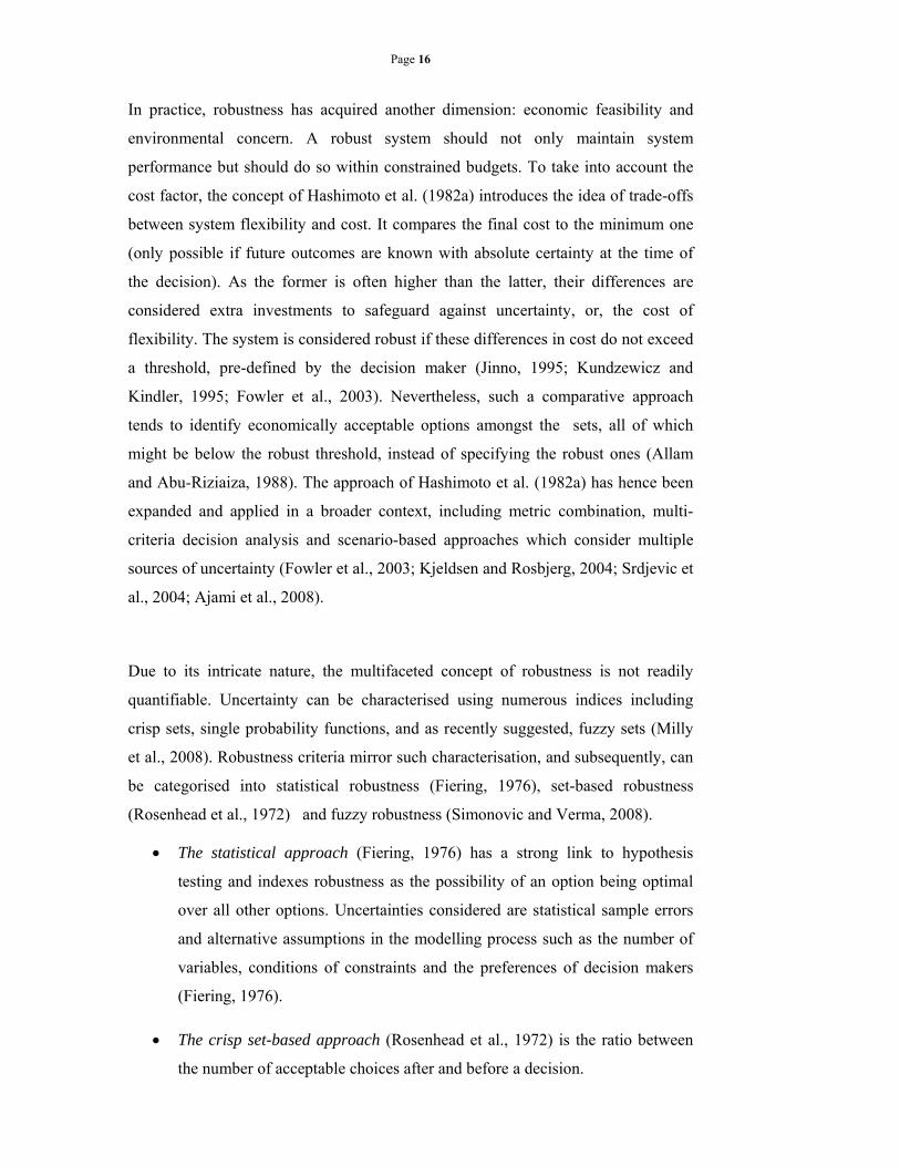
Page 16
In practice, robustness has acquired another dimension: economic feasibility and
environmental concern. A robust system should not only maintain system
performance but should do so within constrained budgets. To take into account the
cost factor, the concept of Hashimoto et al. (1982a) introduces the idea of trade-offs
between system flexibility and cost. It compares the final cost to the minimum one
(only possible if future outcomes are known with absolute certainty at the time of
the decision). As the former is often higher than the latter, their differences are
considered extra investments to safeguard against uncertainty, or, the cost of
flexibility. The system is considered robust if these differences in cost do not exceed
a threshold, pre-defined by the decision maker (Jinno, 1995; Kundzewicz and
Kindler, 1995; Fowler et al., 2003). Nevertheless, such a comparative approach
tends to identify economically acceptable options amongst the sets, all of which
might be below the robust threshold, instead of specifying the robust ones (Allam
and Abu-Riziaiza, 1988). The approach of Hashimoto et al. (1982a) has hence been
expanded and applied in a broader context, including metric combination, multi-
criteria decision analysis and scenario-based approaches which consider multiple
sources of uncertainty (Fowler et al., 2003; Kjeldsen and Rosbjerg, 2004; Srdjevic et
al., 2004; Ajami et al., 2008).
Due to its intricate nature, the multifaceted concept of robustness is not readily
quantifiable. Uncertainty can be characterised using numerous indices including
crisp sets, single probability functions, and as recently suggested, fuzzy sets (Milly
et al., 2008). Robustness criteria mirror such characterisation, and subsequently, can
be categorised into statistical robustness (Fiering, 1976), set-based robustness
(Rosenhead et al., 1972) and fuzzy robustness (Simonovic and Verma, 2008).
The statistical approach (Fiering, 1976) has a strong link to hypothesis
testing and indexes robustness as the possibility of an option being optimal
over all other options. Uncertainties considered are statistical sample errors
and alternative assumptions in the modelling process such as the number of
variables, conditions of constraints and the preferences of decision makers
(Fiering, 1976).
The crisp set-based approach (Rosenhead et al., 1972) is the ratio between
the number of acceptable choices after and before a decision.
Page 17
The fuzzy set approach (El-Baroudy and Simonovic, 2004) compares the risk
of system failure after and before a decision by examining the overlapping
region between the operating system state (e.g. water supplies) and the
failure region (or region of high risks) (El-Baroudy and Simonovic, 2004).
True to their predecessors, the current interpretations of robustness emphasise the
reliability of options and flexibility of the whole system. The following section
outlines several approaches that follow this chain of thought.
This approach arguably dominates the water resource research literature (Ray et al.;
Watkins and McKinney, 1995; Goodwin and Wright, 2001; Chung et al., 2009) and
combines the approaches of robust statistics, robust control theory, machine learning
and robust linear and convex optimisation (Ben-Tal et al., 2009). This set-based and
deterministic approach mainly deals with bounded uncertainty, that is, unknown
distributions of uncertainty but (assumed to be) known intervals containing the value
of interest (Olston and Mackinlay, 2002). Water planning issues are formulated as
linear or dynamic programming (LP/DP) optimisation problems under sets of soft
and hard constraints. The optimisation model has to satisfy all hard constraints; it
can violate soft constraints but would be penalised in the objective function. The
solutions selected can either be feasible or optimal, meaning they satisfy the
constraints or are the best option within the considered uncertainty domain (Ben-Tal
et al., 2009). Robust optimisation explicitly explores the link between the geometry
of uncertainty and robust options. In order for the optimisation to be meaningful, the
set of feasible solutions is often required to be convex. The characterisation of the
uncertainty set U can be further specified to encompass specific uncertainty of
perturbation, probabilistic distributions, or relaxed-representation of normal
distributions (the ellipsoidal set) of the coefficient sets.
In the context of water resources research, this methodology has been applied on
both investment and operational decisions (Ray et al.; Watkins and McKinney,
2.3.2. Robustness in water resources planning
2.3.2.1.Robust optimisation
Page 18
1995; Watkins Jr, 1997). Robust options contain robust optimal and robust feasible
options, selected by specifying constraints such as minimal cost and feasible system
reliability (Watkins Jr, 1997). The method offers flexibility in incorporating multi-
criteria analysis but can potentially be computationally demanding, due to its highly
structured and detailed uncertainty characterisations (Ben-Tal and Nemirovski,
2002). The method is most employed to explore alternative input data and model
parameters, uncertainties of which arise from system disturbance and future
changes.
Real options analysis is a decision technique that focuses explicitly on the sequential
nature of decision making. It concerns future options and actively plans for the
prospect of new options. While not referring directly to the concept of robustness,
the method relies on analysis of flexibility and costs of options, and thus can be seen
as a more extended and comprehensive analysis compared to the approach of
Hashimoto et al. (1982a). In more recent studies, the approach has been analysed in
the context of robust decision analysis (Mahnovski, 2006) and climate risk
management (Beare, 2007). The methodology quantifies the cost and added value of
flexibility based on net present values (NPVs). Originally coined by Myer (1984),
the term “real option” was used in finance theory to include the opportunity cost of
options and to value the cost of flexibility (Watkins Jr, 1997; Wang and De
Neufville, 2004). In its original form, the method was used to determine whether to
invest now or wait. When translated into a water resource-planning context, the
method is used to select discrete decisions and the time of action. For instance,
Gersonius et al. (2010) employ real option analysis to decide a feasible option for
sequential levee enhancement. Assuming that option effectiveness will decline with
time, the study investigated various scenarios of option implementation and their
associating cost and performance. As a result, the design was kept flexible to allow
switching to new options when new information becomes available in the next
planning window (Figure 2.1).
2.3.2.2.Real Options Analysis
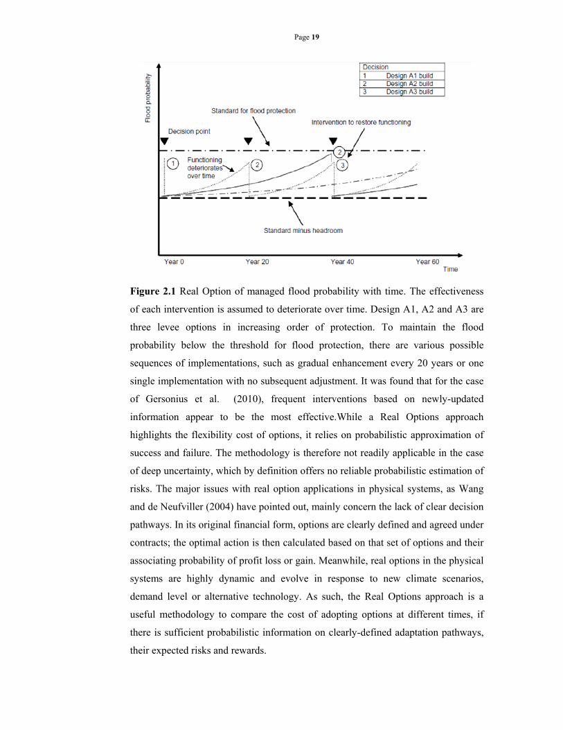
Page 19
Figure 2.1 Real Option of managed flood probability with time. The effectiveness
of each intervention is assumed to deteriorate over time. Design A1, A2 and A3 are
three levee options in increasing order of protection. To maintain the flood
probability below the threshold for flood protection, there are various possible
sequences of implementations, such as gradual enhancement every 20 years or one
single implementation with no subsequent adjustment. It was found that for the case
of Gersonius et al. (2010), frequent interventions based on newly-updated
information appear to be the most effective.While a Real Options approach
highlights the flexibility cost of options, it relies on probabilistic approximation of
success and failure. The methodology is therefore not readily applicable in the case
of deep uncertainty, which by definition offers no reliable probabilistic estimation of
risks. The major issues with real option applications in physical systems, as Wang
and de Neufviller (2004) have pointed out, mainly concern the lack of clear decision
pathways. In its original financial form, options are clearly defined and agreed under
contracts; the optimal action is then calculated based on that set of options and their
associating probability of profit loss or gain. Meanwhile, real options in the physical
systems are highly dynamic and evolve in response to new climate scenarios,
demand level or alternative technology. As such, the Real Options approach is a
useful methodology to compare the cost of adopting options at different times, if
there is sufficient probabilistic information on clearly-defined adaptation pathways,
their expected risks and rewards.
Page 20
2.3.2.3.Info-gap decision theory
The info-gap approach iteratively investigates system performance as system
parameters or descriptions deviate from “best estimates”, provided by expert
judgment or nominal description (Ben-Haim, 2001; Hall, 2003). This reliance on
central tendency is in line with certain practice observed in various decision makers
(Keeney and Raiffa, 1993), who may be more experienced and ready to start the
analysis with central tendency rather than with uncertainty boundaries (Ben-Haim,
2001; Kriegler et al., 2009). The procedure of info-gap starts by determining the
system equation, which describes the linkage among major system components. This
nominal model is an approximation of an actual function of system state
r(x,t,w), which remains unknown. An info-gap uncertainty model:
, ̌ , , : | , , ̃ , , | , 0
Equation 2.1
is developed as a set of function values around the nominal function with α being the
uncertainty parameter. This set is then expanded to explore the ability of
management options that govern the system to meet a certain performance criteria as
uncertainty grows. In info-gap decision theory, “robustness” (the ability to withstand
pernicious change-as defined by the theory) and “opportuness” (the potential for
propitious outcomes) are assessed in reference to the potential deviation from the
“best estimates”. Robustness is displayed and analysed in the form of a robustness
function, which indicates “the greatest level of uncertainty at which failure cannot
occur” (Ben-Haim, 2006). Opportuneness is displayed and analysed in an opposite
function that reveals the lowest level of uncertainty that offers windfall gain. Thus,
the robustness and opportunity of each option can be evaluated and ranked based on
the preference of decision makers, with the general aims being options with high
robustness and low opportuness:
max :
(robustness)
Equation 2.2
min :
(opportuneness)
Equation 2.3
Page 21
As the method uses an uncertainty threshold α to define the domain in which an
option is robust, the uncertainty model used in Info-Gap has to be convex, that is,
the set of models with a smaller deviation α1 should be contained within that of
deviation α2 if α1<α2. While such an assumption might be self-evident in certain
systems (Beven, 2008), there is a need to investigate further specific behaviours of
water planning systems and options, particularly in the case of interactions within
sets of options.
In practice, Hine and Hall (2010) applied Info-gap decision theory on flood
mitigation options to consider the timing, value and uncertainty robustness of each
option (Figure 2.2). If a preference reversal occurs, decision-makers may trade
higher performance for resistance to uncertainty. This graphic portrayal allows
decision makers to adjust their performance criteria and in this sense Info-Gap
theory dispels two forms of determinacy: a pre-determined probability distribution
of potential outcomes and pre-determined performance criteria to be met. In climate
change adaptation studies, Info-Gap theory can assess the varying outcomes due to
changes of model parameters, structures or future scenarios that deviate from the
current state or the “best estimate” scenario of the future (Milly et al., 2008).
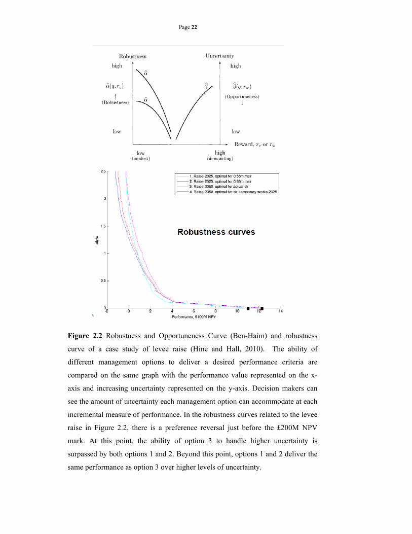
Page 22
Figure 2.2 Robustness and Opportuneness Curve (Ben-Haim) and robustness
curve of a case study of levee raise (Hine and Hall, 2010). The ability of
different management options to deliver a desired performance criteria are
compared on the same graph with the performance value represented on the x-
axis and increasing uncertainty represented on the y-axis. Decision makers can
see the amount of uncertainty each management option can accommodate at each
incremental measure of performance. In the robustness curves related to the levee
raise in Figure 2.2, there is a preference reversal just before the £200M NPV
mark. At this point, the ability of option 3 to handle higher uncertainty is
surpassed by both options 1 and 2. Beyond this point, options 1 and 2 deliver the
same performance as option 3 over higher levels of uncertainty.
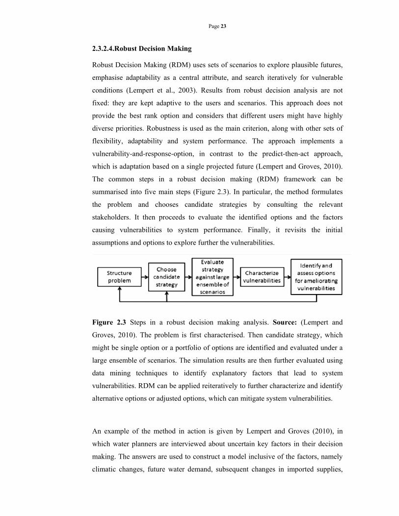
Page 23
Robust Decision Making (RDM) uses sets of scenarios to explore plausible futures,
emphasise adaptability as a central attribute, and search iteratively for vulnerable
conditions (Lempert et al., 2003). Results from robust decision analysis are not
fixed: they are kept adaptive to the users and scenarios. This approach does not
provide the best rank option and considers that different users might have highly
diverse priorities. Robustness is used as the main criterion, along with other sets of
flexibility, adaptability and system performance. The approach implements a
vulnerability-and-response-option, in contrast to the predict-then-act approach,
which is adaptation based on a single projected future (Lempert and Groves, 2010).
The common steps in a robust decision making (RDM) framework can be
summarised into five main steps (Figure 2.3). In particular, the method formulates
the problem and chooses candidate strategies by consulting the relevant
stakeholders. It then proceeds to evaluate the identified options and the factors
causing vulnerabilities to system performance. Finally, it revisits the initial
assumptions and options to explore further the vulnerabilities.
Figure 2.3 Steps in a robust decision making analysis. Source: (Lempert and
Groves, 2010). The problem is first characterised. Then candidate strategy, which
might be single option or a portfolio of options are identified and evaluated under a
large ensemble of scenarios. The simulation results are then further evaluated using
data mining techniques to identify explanatory factors that lead to system
vulnerabilities. RDM can be applied reiteratively to further characterize and identify
alternative options or adjusted options, which can mitigate system vulnerabilities.
An example of the method in action is given by Lempert and Groves (2010), in
which water planners are interviewed about uncertain key factors in their decision
making. The answers are used to construct a model inclusive of the factors, namely
climatic changes, future water demand, subsequent changes in imported supplies,
2.3.2.4.Robust Decision Making
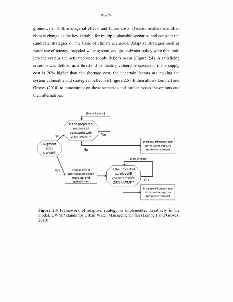
Page 24
groundwater shift, managerial effects and future costs. Decision-makers identified
climate change as the key variable for multiple plausible scenarios and consider the
candidate strategies on the basis of climate scenarios. Adaptive strategies such as
water-use efficiency, recycled-water system, and groundwater policy were then built
into the system and activated once supply deficits occur (Figure 2.4). A satisficing
criterion was defined as a threshold to identify vulnerable scenarios: if the supply
cost is 20% higher than the shortage cost, the uncertain factors are making the
system vulnerable and strategies ineffective (Figure 2.5). It then allows Lempert and
Groves (2010) to concentrate on these scenarios and further assess the options and
their alternatives.
Figure 2.4 Framework of adaptive strategy as implemented iteratively in the model. UWMP stands for Urban Water Management Plan (Lempert and Groves, 2010)
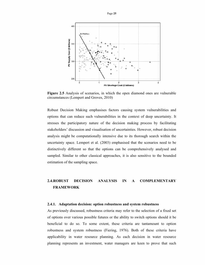
Page 25
Figure 2.5 Analysis of scenarios, in which the open diamond ones are vulnerable circumstances (Lempert and Groves, 2010)
Robust Decision Making emphasises factors causing system vulnerabilities and
options that can reduce such vulnerabilities in the context of deep uncertainty. It
stresses the participatory nature of the decision making process by facilitating
stakeholders’ discussion and visualisation of uncertainties. However, robust decision
analysis might be computationally intensive due to its thorough search within the
uncertainty space. Lempert et al. (2003) emphasised that the scenarios need to be
distinctively different so that the options can be comprehensively analysed and
sampled. Similar to other classical approaches, it is also sensitive to the bounded
estimation of the sampling space.
2.4.ROBUST DECISION ANALYSIS IN A COMPLEMENTARY
FRAMEWORK
2.4.1. Adaptation decision: option robustness and system robustness
As previously discussed, robustness criteria may refer to the selection of a fixed set
of options over various possible futures or the ability to switch options should it be
beneficial to do so. To some extent, these criteria are tantamount to option
robustness and system robustness (Fiering, 1976). Both of these criteria have
applicability in water resource planning. As each decision in water resource
planning represents an investment, water managers are keen to prove that such
Page 26
investment is worthwhile and the option is robust, particularly when the capital and
operation cost are high. Infrastructure options such as reservoir, nevertheless,
require a significant amount of time and effort in preparing proposals, impact
assessments and preparation. A reservoir’s capacity, operation rules and expected
operation duration are largely determined by initial infrastructure design; switching
away from initial designs at a later stage may become costly. While option
robustness ensures that the decision remains correct within a wide range of futures,
there is a risk of mal-adaptation due to possible lack of system flexibility. In that
context, system robustness becomes relevant. Climate change scenarios introduce a
wide and complex range of possible futures for water systems to adapt to,
subsequently make adaptive and robust options difficult to achieve. If adaptation
methods are flexible and non-capital intensive, future option switching or system
enhancement will be more readily implemented.
The comparison highlights the diversity of uncertainty tackled and robustness
criteria in various methodologies. As Table 2.1 depicts, these methods may concern
the range of options before and after a decision (fuzzy robustness), trade-offs
between performance, flexibility and cost (classical robustness and real options),
likelihood of option optimality (statistical robustness, robust optimisation), overall
vulnerabilities to changes in system estimates/characterisation (info-gap decision
theory), or inherent vulnerable components of the system itself. These methods
differ significantly in uncertainty characterisation: the group of Classical
Robustness, Statistical Robustness, and Real Options use a single probabilistic
description; Fuzzy Robustness use fuzzy logic while Info-gap Decision Theory and
RDM are scenario-based.
The main objectives of the methodologies are one of the main foci of this chapter.
Classical robustness and statistical robustness both emphasise the low possibility of
the conclusion being wrong based on reliable probability estimations of the system
and system responses. Meanwhile, fuzzy robustness relaxes the requirement for
probability estimations and allows buffer conditions between system failure and
2.4.2. Comparison of methodologies
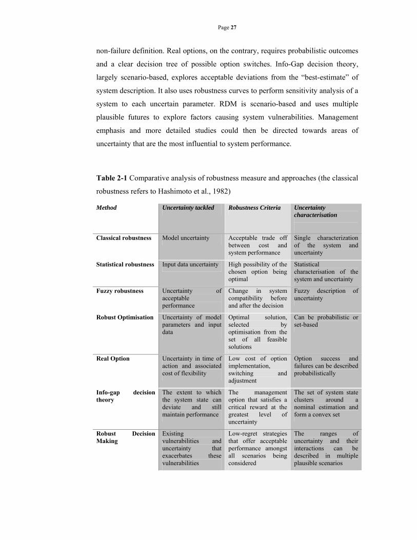
Page 27
non-failure definition. Real options, on the contrary, requires probabilistic outcomes
and a clear decision tree of possible option switches. Info-Gap decision theory,
largely scenario-based, explores acceptable deviations from the “best-estimate” of
system description. It also uses robustness curves to perform sensitivity analysis of a
system to each uncertain parameter. RDM is scenario-based and uses multiple
plausible futures to explore factors causing system vulnerabilities. Management
emphasis and more detailed studies could then be directed towards areas of
uncertainty that are the most influential to system performance.
Table 2-1 Comparative analysis of robustness measure and approaches (the classical
robustness refers to Hashimoto et al., 1982)
Method Uncertainty tackled Robustness Criteria Uncertainty characterisation
Classical robustness Model uncertainty Acceptable trade off between cost and system performance
Single characterization of the system and uncertainty
Statistical robustness Input data uncertainty High possibility of the chosen option being optimal
Statistical characterisation of the system and uncertainty
Fuzzy robustness Uncertainty of acceptable performance
Change in system compatibility before and after the decision
Fuzzy description of uncertainty
Robust Optimisation Uncertainty of model parameters and input data
Optimal solution, selected by optimisation from the set of all feasible solutions
Can be probabilistic or set-based
Real Option Uncertainty in time of action and associated cost of flexibility
Low cost of option implementation, switching and adjustment
Option success and failures can be described probabilistically
Info-gap decision theory
The extent to which the system state can deviate and still maintain performance
The management option that satisfies a critical reward at the greatest level of uncertainty
The set of system state clusters around a nominal estimation and form a convex set
Robust Decision Making
Existing vulnerabilities and uncertainty that exacerbates these vulnerabilities
Low-regret strategies that offer acceptable performance amongst all scenarios being considered
The ranges of uncertainty and their interactions can be described in multiple plausible scenarios
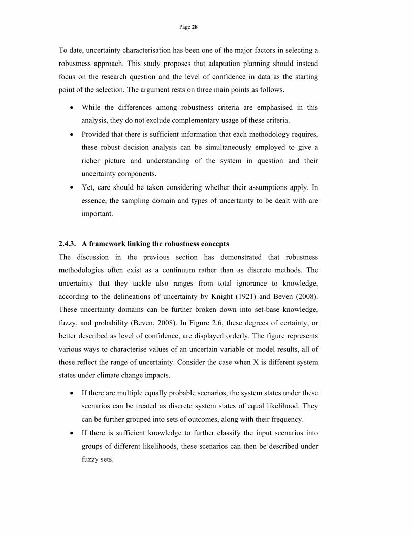
Page 28
To date, uncertainty characterisation has been one of the major factors in selecting a
robustness approach. This study proposes that adaptation planning should instead
focus on the research question and the level of confidence in data as the starting
point of the selection. The argument rests on three main points as follows.
While the differences among robustness criteria are emphasised in this
analysis, they do not exclude complementary usage of these criteria.
Provided that there is sufficient information that each methodology requires,
these robust decision analysis can be simultaneously employed to give a
richer picture and understanding of the system in question and their
uncertainty components.
Yet, care should be taken considering whether their assumptions apply. In
essence, the sampling domain and types of uncertainty to be dealt with are
important.
2.4.3. A framework linking the robustness concepts
The discussion in the previous section has demonstrated that robustness
methodologies often exist as a continuum rather than as discrete methods. The
uncertainty that they tackle also ranges from total ignorance to knowledge,
according to the delineations of uncertainty by Knight (1921) and Beven (2008).
These uncertainty domains can be further broken down into set-base knowledge,
fuzzy, and probability (Beven, 2008). In Figure 2.6, these degrees of certainty, or
better described as level of confidence, are displayed orderly. The figure represents
various ways to characterise values of an uncertain variable or model results, all of
those reflect the range of uncertainty. Consider the case when X is different system
states under climate change impacts.
If there are multiple equally probable scenarios, the system states under these
scenarios can be treated as discrete system states of equal likelihood. They
can be further grouped into sets of outcomes, along with their frequency.
If there is sufficient knowledge to further classify the input scenarios into
groups of different likelihoods, these scenarios can then be described under
fuzzy sets.
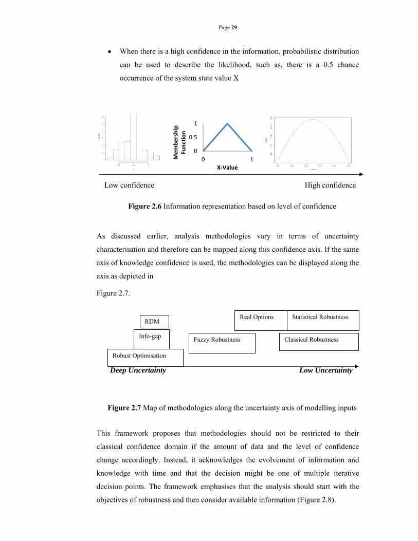
Page 29
When there is a high confidence in the information, probabilistic distribution
can be used to describe the likelihood, such as, there is a 0.5 chance
occurrence of the system state value X
Low confidence High confidence
Figure 2.6 Information representation based on level of confidence
As discussed earlier, analysis methodologies vary in terms of uncertainty
characterisation and therefore can be mapped along this confidence axis. If the same
axis of knowledge confidence is used, the methodologies can be displayed along the
axis as depicted in
Figure 2.7.
Deep Uncertainty Low Uncertainty
Figure 2.7 Map of methodologies along the uncertainty axis of modelling inputs
This framework proposes that methodologies should not be restricted to their
classical confidence domain if the amount of data and the level of confidence
change accordingly. Instead, it acknowledges the evolvement of information and
knowledge with time and that the decision might be one of multiple iterative
decision points. The framework emphasises that the analysis should start with the
objectives of robustness and then consider available information (Figure 2.8).
0
0.5
1
0 1Membership
Function
X‐Value
Classical Robustness
Real Options
Info-gap
RDM
Fuzzy Robustness
Robust Optimisation
Statistical Robustness
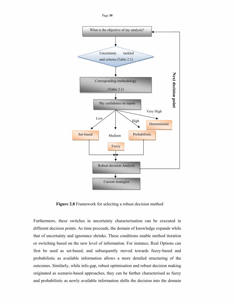
Page 30
Figure 2.8 Framework for selecting a robust decision method
Furthermore, these switches in uncertainty characterisation can be executed in
different decision points. As time proceeds, the domain of knowledge expands while
that of uncertainty and ignorance shrinks. These conditions enable method iteration
or switching based on the new level of information. For instance, Real Options can
first be used as set-based, and subsequently moved towards fuzzy-based and
probabilistic as available information allows a more detailed structuring of the
outcomes. Similarly, while info-gap, robust optimisation and robust decision making
originated as scenario-based approaches, they can be further characterised as fuzzy
and probabilistic as newly available information shifts the decision into the domain
What is the objective of my analysis?
Uncertainty tackled
and criteria (Table 2.1)
Corresponding methodology
(Table 2.1)
My confidence on inputs
High Low
Medium Probabilistic
Fuzzy
Set-based
Robust decision Analysis
Current strategies
Next d
ecision p
oint
Very High
Deterministic
Page 31
of less deep uncertainty. As such, at each new decision point, the user can choose to
reiterate their previous methodology or adopt a new method to suit their current
level of uncertainty. The shift will also reflect their priority of which kind of
uncertainty to explore (refer to Table 2-1).
2.5.CONCLUSION
This chapter has reviewed various robust decision methodologies and their
associated criteria. It demonstrates that each of these methods follows different
underlying assumptions and characterizes different uncertainty types and levels.
Recent robustness criteria stem from classical groups of statistical-base, rough set-
base or fuzzy-based concept. Such diversion in uncertainty descriptions have been
captured in Table 2-1 and Figure 2.4, in which the type of uncertainty
characterisation and the evolution of uncertainty level are illustrated. The classical
robustness emphasises trade-offs between cost and system performance, and at the
same time requires low-regret for the selected decision. Fuzzy robustness is an
extension of classical set-based robustness, with the improvements being the usage
of likelihood/membership function and a more flexible definition of system failures.
Robust optimisation formulates the issue as an optimisation problem under set of
hard and soft constraints, the solutions of which are deemed robust feasible and
robust optimal solutions. Real option analysis offers a comprehensive analysis of the
cost of flexibility, with the limitation being its adherence to probabilistic
assumptions. Info-gap Decision Theory focuses on strategies that can achieve the
lowest critical performance over the highest level of deviation from the central
tendency, or “best-estimate”, while RDM targets factors causing vulnerabilities in
the system in question. Overall, the differences in assumptions and methods of these
approaches do not exclude their complementary deployment. Furthermore, such
deployment can be beneficial as it allows deeper understanding of the system and
adaptation options.
It is also recognised that robustness can refer to option robustness or system
robustness. The former emphasises the superiority of the chosen option across a
Page 32
wide range of scenarios while the latter puts more weight on option switching. It
might be possible to have a robust option that does not reduce the possibility of
option switching or retrofitting. However, in long-term decisions, system robustness
should be prioritised to avoid to mal-adaptation and costly lock-in. It is thus
suggested that legislation frameworks and guidelines to the water industry should
place more emphasis on system robustness and flexibility. The paper illustrates that
water planning should select acceptable options that satisfy the robustness criteria
rather than optimal options which might be susceptible to greater uncertainty.
Finally, the chapter presents a decision framework linking robustness methodologies
based on their classical definition and uncertainty characterisation. The framework
emphasises the utility of methodologies by choosing their objectives as the starting
point. It also expands the methodologies into uncertainty domains that are not
covered in the original methodology description, thus enhances their usage under
other levels of uncertainty. The framework considers decision making as a dynamic
process, in which knowledge changes with time and decisions can be revisited in
future planning cycles. Overall, the framework helps to clearly define the objective
of various robust decision methodologies and structurally tackle uncertainty attached
in planning decisions. This framework helps compare and contrast the related
methodologies to distinguish existing robustness approaches. This literature review-
based framework therefore highlights the principles of robustness that will be the
basis for the Methodology chapter, which targets key features of the robustness
concept in a multi-criteria robust decision making context.

Page 33
33
Chapter 3. METHODOLOGY
This chapter presents the analysis framework used in this study. The framework is a
systematic process that links and analyses component uncertainty of climate-related
planning decisions. The chapter focuses on the main structure and linking logic amongst
the components; Chapters 5, 6, 7 and 8 will further explain specific treatments of each
uncertainty component. Section 3.1 first starts with a brief overview of current
uncertainty assessment frameworks and their drawbacks. Section 3.2 then proceeds to
describe the aims, structure and key points of the framework proposed and used in this
study. The chapter concludes with the specific structure and a flow chart of the
methodology, which are summarised in Section 3.3 that also serves as a roadmap of
subsequent chapters.
3.1.LINKING AND INTEGRATING UNCERTAINTY
3.1.1. ‘Top-down’ and ‘bottom-up’ approaches
As Chapter 2 illustrates, methodologies of uncertainty assessment are scattered in
various research literatures, from mathematics and operational research to climate
impact studies. In climate adaptation policy, frameworks linking these methodologies
often either starts from the climate end or the decision end, described as the ‘top-down’
and ‘bottom-up’ approaches (Dessai and Hulme, 2004). The ‘top-down’ approach, as
suggested by the Intergovernmental Panel for Climate Change (IPCC), designs
adaptation policy to alleviate the vulnerabilities exposed by climate uncertainty (Wilby
and Dessai). Meanwhile, the ‘bottom-up’ approach constructs policy based on the
available adaptive capacity and resources- the limiting factors of possible adaptation
actions (Smit and Wandel, 2006). These two complementary approaches answer two
Page 34
34
different questions: the former targets the climate uncertainty envelope while the latter
tackles the social adaptive boundary.
Tying together the impact and response end, both of these approaches provide the
context and scenarios for adaptation policy analysis. While traditionally, policy analysis
has considered multiple scenarios and contexts, the inherent uncertainty in climate
change impacts rapidly expands future projections into thousands of scenarios and
possibilities. This high level of uncertainty requires a move from scenario-based to risk-
based approaches (Jones, 2001; Klinke and Renn, 2002; Keller et al., 2005; Cowell et
al., 2006). These risk-based approaches are naturally closer to the ‘bottom-up’ approach
than the ‘top-down’ one, as vulnerability is context and system-dependent. They focus
on impact-scale vulnerabilities and decision-relevant conditions, for instance rainfall
and temperature patterns that lead to crop failures, water deficit or ecosystem damages
(Risbey, 1998; Liverman, 1999; Lempert and Groves, 2010; Prudhomme et al., 2010;
Brown et al., 2011; Brown et al., 2012). These conditions are then used to analyse either
key risks projected in the climate model outputs (Brown et al., 2012), or possible
enhancements of the area’s current coping capacity (Yohe and Tol, 2002; Füssel and
Klein, 2006; Thomalla et al., 2006; Füssel, 2007).
The basic structures of selected methodologies are depicted in Figure 3.1. The
traditional ‘top-down’ starts from the global or regional climate models, which output
data spatially as square grid boxes of 50x50 to 300x300 km2. Since this scale is too
coarse for most study areas, the data often require further modelling or statistical
analysis. These ‘downscaled’ climate projections then provide input data for the impact
models, which generate scenarios for vulnerability analysis. In contrast, the ‘bottom-up’
Robust Decision Making (RDM) and Decision-Scaling start from the options (Lempert
and Groves, 2010).
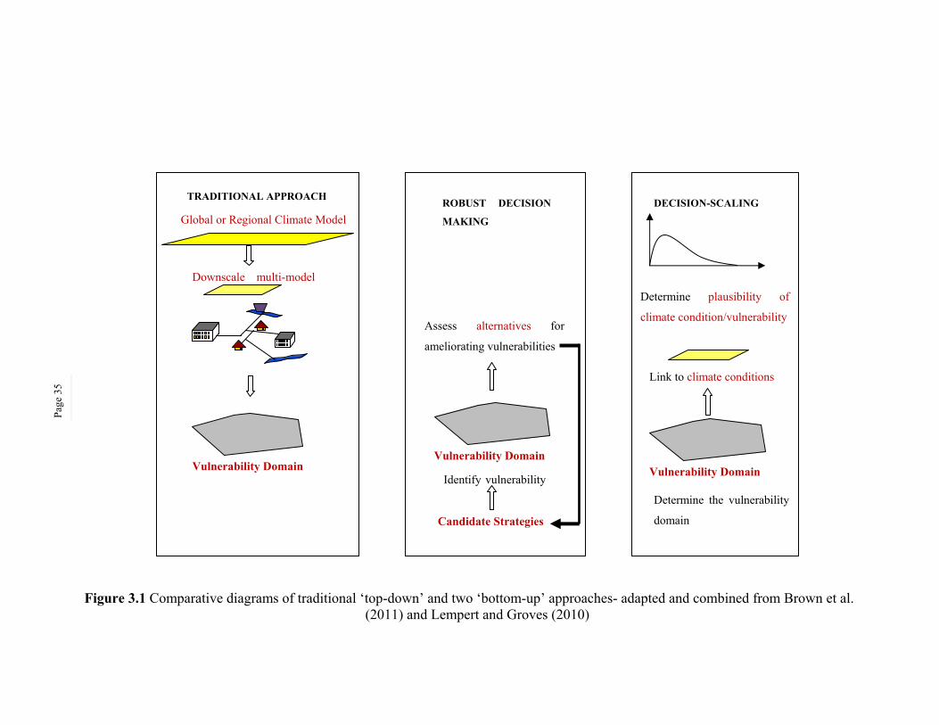
Pag
e 35
Figure 3.1 Comparative diagrams of traditional ‘top-down’ and two ‘bottom-up’ approaches- adapted and combined from Brown et al. (2011) and Lempert and Groves (2010)
Link to climate conditions
Determine plausibility of
climate condition/vulnerability
DECISION-SCALING
Find
whether
system is
vulnerable
for these
Downscale multi-model
Generate a
few water
supply
Global or Regional Climate Model
Vulnerability Domain
TRADITIONAL APPROACH
Assess alternatives for
ameliorating vulnerabilities
Identify vulnerability
Candidate Strategies
ROBUST DECISION
MAKING
Vulnerability Domain
Determine the vulnerability
domain
Vulnerability Domain
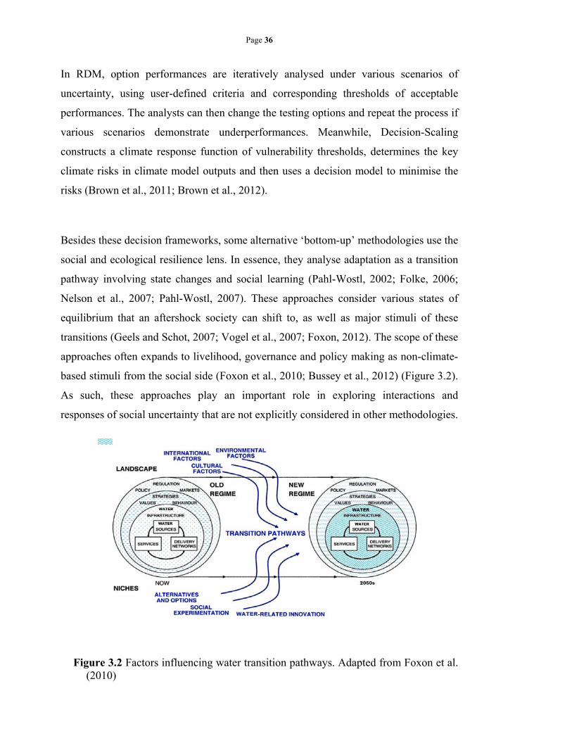
Page 36
In RDM, option performances are iteratively analysed under various scenarios of
uncertainty, using user-defined criteria and corresponding thresholds of acceptable
performances. The analysts can then change the testing options and repeat the process if
various scenarios demonstrate underperformances. Meanwhile, Decision-Scaling
constructs a climate response function of vulnerability thresholds, determines the key
climate risks in climate model outputs and then uses a decision model to minimise the
risks (Brown et al., 2011; Brown et al., 2012).
Besides these decision frameworks, some alternative ‘bottom-up’ methodologies use the
social and ecological resilience lens. In essence, they analyse adaptation as a transition
pathway involving state changes and social learning (Pahl-Wostl, 2002; Folke, 2006;
Nelson et al., 2007; Pahl-Wostl, 2007). These approaches consider various states of
equilibrium that an aftershock society can shift to, as well as major stimuli of these
transitions (Geels and Schot, 2007; Vogel et al., 2007; Foxon, 2012). The scope of these
approaches often expands to livelihood, governance and policy making as non-climate-
based stimuli from the social side (Foxon et al., 2010; Bussey et al., 2012) (Figure 3.2).
As such, these approaches play an important role in exploring interactions and
responses of social uncertainty that are not explicitly considered in other methodologies.
Figure 3.2 Factors influencing water transition pathways. Adapted from Foxon et al. (2010)
Page 37
3.1.2. Bridging approaches: the challenge
Using only the ‘top-down’ or ‘bottom-up’ approach poses problems but bridging these
two approaches is challenging. Focus on either the former or the latter can distract or
misinform decision makers. ‘Top-down’ presents an overwhelming level of uncertainty
in climate projections, many of which are not decision-relevant or highly uncertain on
the impact scale. Meanwhile, ‘bottom-up’ presents a danger of exclusively relying and
focusing on ‘known’ or experienced risks. There exist very few frameworks that can
comprehensively and integrate risk analysis from both ends (Brown et al., 2012)
because of four characteristics of the current approaches.
Firstly, uncertainty at either end is essentially different in forms and governing regimes.
The top-down uncertainty, coming from physical climate models, is often quantified
and shown as projections; meanwhile, adaptation responses are qualitative, fluid and
context-dependent. In linking climate and social impacts, qualitative uncertainty is often
considered in a separate framework, thus impedes the integrated nature of the
uncertainty assessment.
Secondly, both physical and social vulnerability often revolve around the concept of
limits and thresholds, a degree of changes that leads to critical transitions or state shifts
(Pittock and Jones, 2000; Brown et al., 2011). Yet, crossing a threshold does not
automatically prompt adaptation and such thresholds are often hard to determine (Adger
et al., 2009). Responses can also vary widely from a behavioural basis (Grothmann and
Patt, 2005), as risk tolerance differs from individual to individual due to attitudes,
perceptions and decision-making positions (Thompson et al., 1990; Thompson, 2003).
Communication of risk is also a key issue: individuals not only react differently to risks
but also to different visualisation of the same risk (Gettinger et al., 2012).
Thirdly, adaptation responses exhibit non-linear patterns and may evolve to new
information, risks, shocks and surprises. Yet the current approaches largely lack
analysis of multi-state shifts and responses to climate change. This missing aspect is
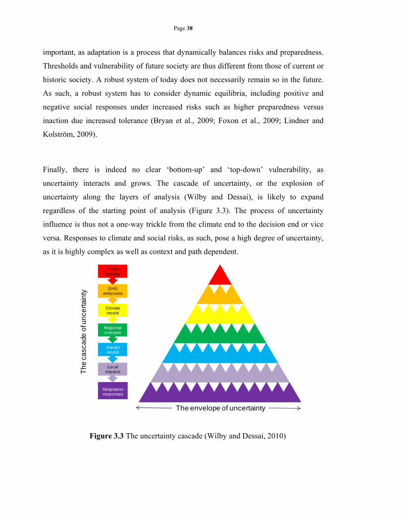
Page 38
important, as adaptation is a process that dynamically balances risks and preparedness.
Thresholds and vulnerability of future society are thus different from those of current or
historic society. A robust system of today does not necessarily remain so in the future.
As such, a robust system has to consider dynamic equilibria, including positive and
negative social responses under increased risks such as higher preparedness versus
inaction due increased tolerance (Bryan et al., 2009; Foxon et al., 2009; Lindner and
Kolström, 2009).
Finally, there is indeed no clear ‘bottom-up’ and ‘top-down’ vulnerability, as
uncertainty interacts and grows. The cascade of uncertainty, or the explosion of
uncertainty along the layers of analysis (Wilby and Dessai), is likely to expand
regardless of the starting point of analysis (Figure 3.3). The process of uncertainty
influence is thus not a one-way trickle from the climate end to the decision end or vice
versa. Responses to climate and social risks, as such, pose a high degree of uncertainty,
as it is highly complex as well as context and path dependent.
Figure 3.3 The uncertainty cascade (Wilby and Dessai, 2010)
Future society
GHG emissions
Climate model
Regional scenario
Impact model
Local impacts
Adaptation responses
The envelope of uncertainty
The
ca
scad
e of
un
cert
aint
y
Page 39
These methodological difficulties translate to the applied side of the decision making
process. In the face of uncertainty, responses to risks include delaying action until
uncertainty is reduced and mal-adaptation- where actions further weaken the coping
capacity (Adger, 2000; Barnett and O’Neill, 2010). Initial adaptive responses might
shift to mal-adaptation and disintegrating trust when the climate risks increase
(Niemeyer et al., 2005). Yet , water planning in practice still shows a high dependency
on historic trends and extreme events (Subak, 2000). Complex decision making tools do
not necessarily help alleviate this state: decision makers may respond sceptically or
become unsure of how to interpret options and projections (Lempert et al., 2003). An
integrated framework of adaptation thus has to efficiently connect uncertainty factors
while additionally informing and interacting with the decision makers on key
information (Jones, 2001).
To sum up, the current lack of an integrated approach in climate impact research results
from inherent differences of uncertainty from the decision and the impact end, problems
in defining adaptation thresholds, and the lack of multistate response analysis. Yet,
‘bottom-up’ and ‘top-down’ uncertainties are linked and a truly connected approach
should include the same key uncertainty regardless of its starting point. These
challenges thus call for an integrated methodology that recognises the changing nature
of adaptation decision making and with less emphasis on the ‘top-down’-‘bottom-up’
diversion.
3.2.THE ROBUST DECISION ANALYSIS FRAMEWORK
3.2.1. Aims and objectives
In dealing with the challenges mentioned above, this study puts forward a framework
that blends relevant uncertainty managements and embraces the changing nature of
adaptation decisions. The scope of the framework is to tackle integrated uncertainty in
drought planning decisions under a changing climate. This framework assists decision
Page 40
makers in identifying potential pathways that can reduce financial costs and
vulnerability to climate risks. The main objectives of the framework is therefore
To improve computational efficiency of RDM by combining with Robust
Optimisation.
To make decision makers aware of potential trade-offs and uncertainty in
adaptation decisions
To facilitate decision making via multi-criteria risk visualisation, so that
decision makers can choose options that match their initial criteria or accept a
certain risk level given the uncertainty
To analyse temporal adaptation pathways that prepare the present water system
for climate risks in 2020s, 2030s and 2050s
The uncertainty considered includes climatic, hydrological and water resources
uncertainty. Main methodologies in this study include scenario planning, multi-criteria
analysis and robust decision making. Three main features characterise the framework.
Firstly, the framework integrates various uncertainty factors that are linked by the
‘knock-on’ effects of climate change impacts. Secondly, it couples multi-criteria
analysis and scenario planning to explore the potential impacts of combined uncertainty.
The framework combines Robust Optimisation and RDM. It improves the
computational effort compared to RDM and provides comparison on sub-optimal
options compared to Robust Optimisation. Thirdly, the framework allows decision-
makers to change their criteria and criteria priorities in response to updated information
or interactions with impact projections. The framework, in support of the study
objectives, aims to transform adaptation decision making from being solution and
problem-oriented into option-oriented. In doing so, it acknowledges that problem
definition and solution selection rest with the decision makers, thus changing in time
and from stakeholder to stakeholder. To facilitate changing objectives and perspectives,
options are interactively displayed for analysis. Through the framework, decision
makers can rethink their adaptation decisions in light of updated information or changes
in their adaptation preferences. The framework, however, does not indicate which
options the decision maker should choose. Its objective is to help the decision makers
analyse and possibly revise choices with an awareness of probable consequences.
Page 41
3.2.2. Structure
This study proposes a study framework that does not revolve around the ‘top-down’ and
‘bottom-up’ debate. It combines simulation with optimisation to improve the efficiency
of option selection. Figure 3.4 presents the steps and characteristics of this framework.
As discussed, it is difficult, even unattainable to comprehensively bridge the physical
and social uncertainty. The proposed framework instead focuses on adaptation
decisions, the outcome of both ‘top-down’ and ‘bottom-up’ vulnerabilities. A robust
decision needs to link physical components and possible patterns of social responses to
climate change, thus has to compromise the vast uncertainties in climate projections and
the specific focus of adaptation at the local scale. In the framework, vulnerabilities are
not characterised as black-or-white boundaries that either trigger failures or require
adaptation. Rather, it is framed as areas of unsatisfactory states or deep uncertainty,
two conditions that the decision makers may want to avoid. The unsatisfactory state
occurs when the system displays characteristics outside of the decision makers’ desired
range; meanwhile, deeply uncertain system is a configuration that might work for only a
few amongst the wide range of possible scenarios.
More importantly, the framework revolves around the interactive and shifting
adaptation preferences, thus makes space for risk negotiation, in which decision makers
either seek additional option(s) to achieve their current risk preference, or accept
another level of risk. This risk acceptance is not tantamount to inaction or non-
adaptation. In many cases, the marginal cost of being insured for a high risk level is
much higher than the marginal benefits; in other cases, there is no option that can
achieve the desired safety level. By being aware of the risk and taking alternative
actions to deal with the risk, decision makers are arguably better informed and more
active in the decision-making process. Furthermore, this interactive step enhances
decision makers’ involvement in choosing the level of risk and adaptation actions. The
framework stresses that decision makers should not feel overwhelmed, outsmarted or
deluded by the complex models in the analysis. Making the decision makers central also
motivates them to feedback on the model performance or explore ‘top-down’ risk
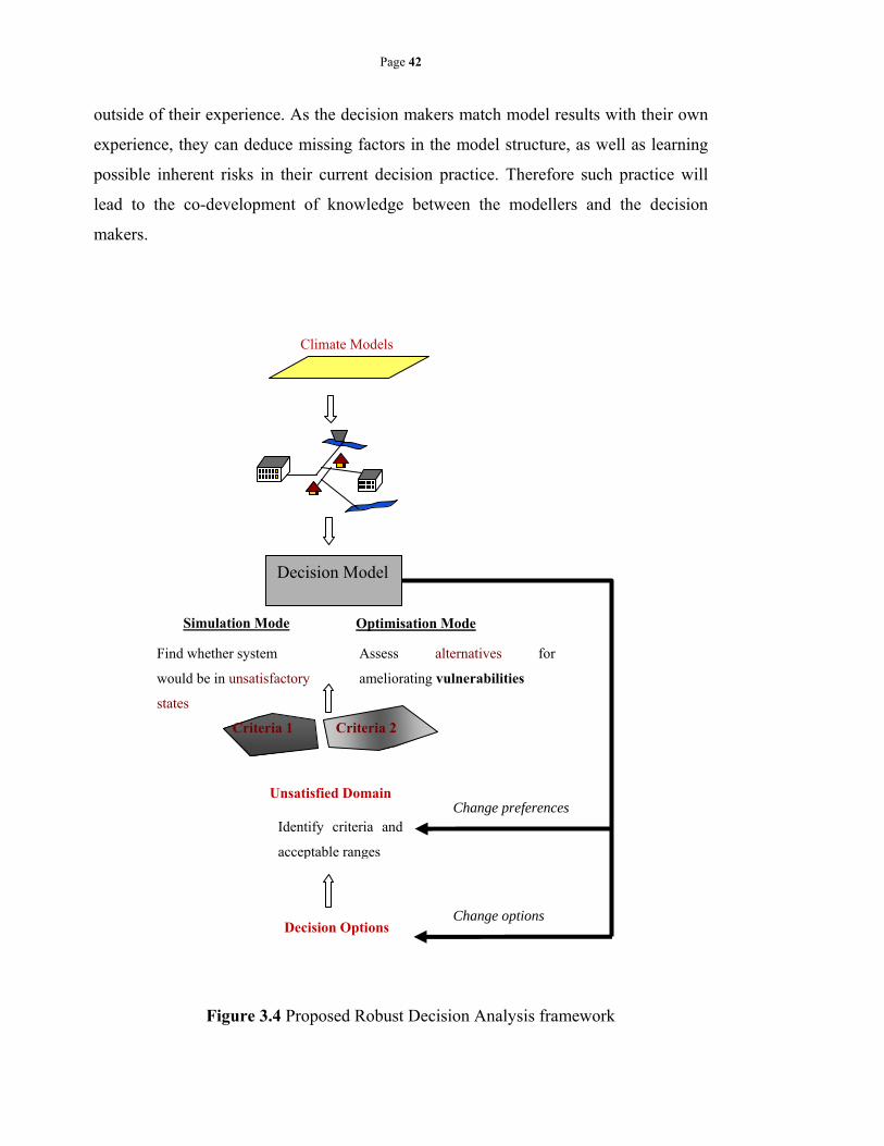
Page 42
outside of their experience. As the decision makers match model results with their own
experience, they can deduce missing factors in the model structure, as well as learning
possible inherent risks in their current decision practice. Therefore such practice will
lead to the co-development of knowledge between the modellers and the decision
makers.
Figure 3.4 Proposed Robust Decision Analysis framework
+
Criteria 1 Criteria 2
Identify criteria and
acceptable ranges
Decision Options
Unsatisfied Domain
Climate Models
Change preferences
Change options
Assess alternatives for
ameliorating vulnerabilities
Find whether system
would be in unsatisfactory
states
Decision Model
Simulation Mode Optimisation Mode
Page 43
In order to address these key points, the proposed framework utilises relevant features
of decision support frameworks mentioned in Section 3.1. In particular, it inherits the
iterative approach of RDM and the efficient and decision-oriented aspects of Decision-
Scaling. The framework differs from Robust Decision Making in two aspects:
Capacity to change criteria and risk acceptance range: In RDM, if the
decision makers are not satisfied with the option performance, they could
further explore other options but could not change their stated decision
thresholds. Robust Decision Analysis instead offers the decision makers two
choices of changing options or their acceptable risk levels. The decision makers
could then investigate the performance of the new options and/or the
consequence of changing the acceptable risk levels.
The optimisation step which preselects potential options: RDM presents a
framework that engages decision makers to iteratively analyse option by option.
Meanwhile, Robust Decision Analysis analyses all available options and their
combinations, therefore could present each option performance in reference to
other options. This process of identifying potential robust options is useful
when the number of options is large and option performance varies greatly
under different climate and water demand scenarios.
Furthermore, it has also improved the Decision-Scaling method in two aspects:
Dynamic sensitive conditions: The iterative structure of Robust Decision
Analysis allows revisiting and adjusting the thresholds of sensitive conditions
(the critical climate conditions influencing planning decisions). Therefore, in
contrast to the static sensitive conditions of Decision-Scaling, the sensitive
conditions of Robust Decision Analysis can be changed in response to new
information from each of the iterations. In essence, the decision makers can
assess whether their planning options and response thresholds have sufficiently
mitigated the risks, and explore other options or thresholds for planning
decisions. Moreover, the discussion regarding threshold and option adjustments
can potentially facilitate communication amongst stakeholders and expose their
different risk averseness. This participatory agreement on the acceptable risk
level is important, as it may lead to further understanding of potential risks each
Page 44
threshold poses for different stakeholders and their acceptability of these risk
levels.
Analysis of option capacity both under perfect information and deep
uncertainty: Decision-Scaling provides the decision makers with the optimal
decisions in different climate conditions. However, it does not identify the
overall risks to the system, given the full set of climate projections. Meanwhile,
Robust Decision Analysis presents individual and overall option performance
under no uncertainty (optimisation mode) and deep uncertainty (simulation
mode). The former mode, similar to Decision-Scaling, identifies the optimal
decision in each scenario and reduces the computational effort compared to
brute force option analysis. The simulation results additionally provide option
performance under uncertainty. It therefore compares not only option capacity,
but also the level of uncertainty at which an option can operate. Under
uncertainty, option performance is determined by various factors, such as
proximity to the shortage hotspots and the lead time for an option to take effect.
Therefore an optimal option for forecasted droughts might be different from
optimal options for sudden drought onset. With Robust Decision Analysis,
decision makers can further consider trade-offs between the general capacity of
options and their ability to perform under uncertainty.
Compared to both Robust Decision Making and Decision-Scaling, the framework also
bears several other minor differences. Firstly, the framework differs in its vulnerability
representation. Both RDM and Decision-Scaling use discrete thresholds, which imply
abrupt decision switches once the thresholds are crossed. Meanwhile, the framework, as
discussed above, considers decisions driven by a continuous range of conditions. It
therefore does not automatically assess the appropriateness of options in the adaptation
plans; but instead let the decision makers compare option costs and performance and
decide on options that match their risk tolerance. Secondly the framework explicitly
emphasises the multi-criteria aspect in its analysis and visualisation. While various
methodologies rely on the aggregated weighted sum of normalised criteria, the
framework utilises an integrated methodology that analyse criteria as independent
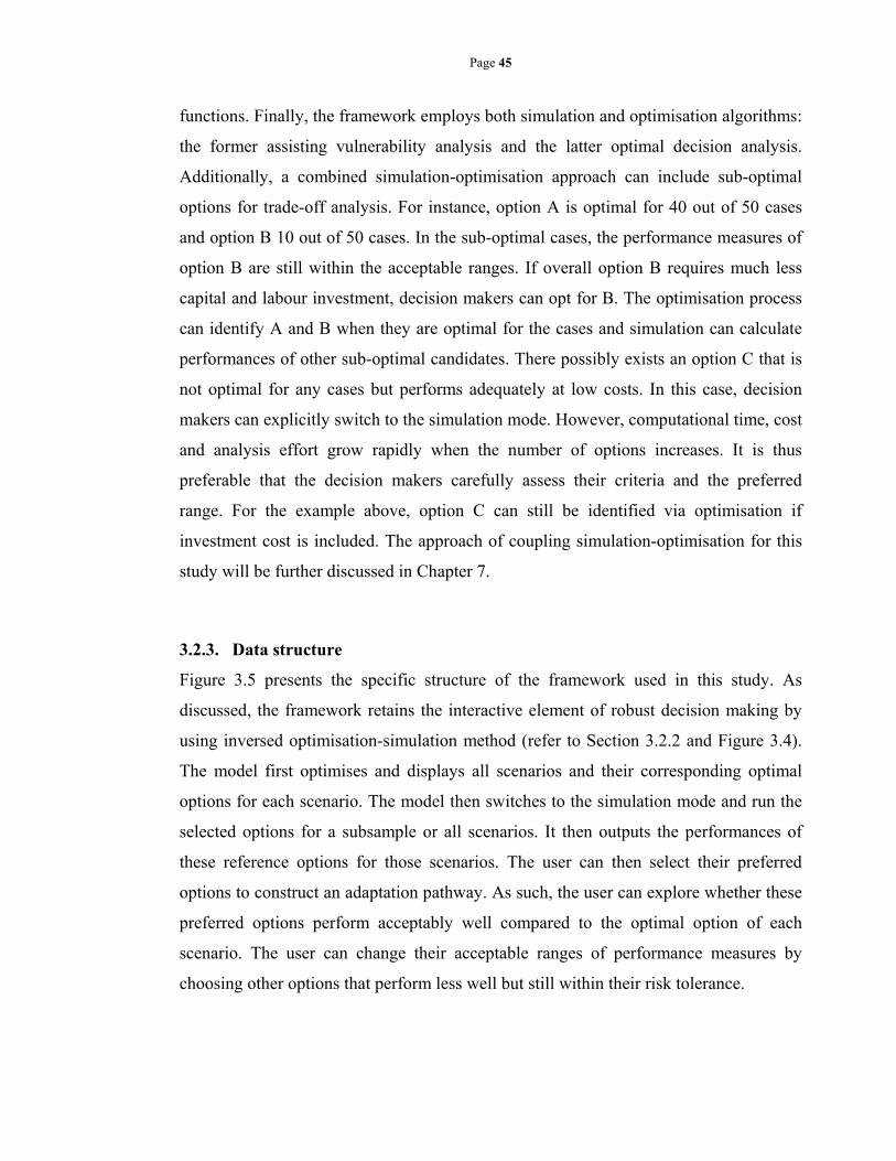
Page 45
functions. Finally, the framework employs both simulation and optimisation algorithms:
the former assisting vulnerability analysis and the latter optimal decision analysis.
Additionally, a combined simulation-optimisation approach can include sub-optimal
options for trade-off analysis. For instance, option A is optimal for 40 out of 50 cases
and option B 10 out of 50 cases. In the sub-optimal cases, the performance measures of
option B are still within the acceptable ranges. If overall option B requires much less
capital and labour investment, decision makers can opt for B. The optimisation process
can identify A and B when they are optimal for the cases and simulation can calculate
performances of other sub-optimal candidates. There possibly exists an option C that is
not optimal for any cases but performs adequately at low costs. In this case, decision
makers can explicitly switch to the simulation mode. However, computational time, cost
and analysis effort grow rapidly when the number of options increases. It is thus
preferable that the decision makers carefully assess their criteria and the preferred
range. For the example above, option C can still be identified via optimisation if
investment cost is included. The approach of coupling simulation-optimisation for this
study will be further discussed in Chapter 7.
3.2.3. Data structure
Figure 3.5 presents the specific structure of the framework used in this study. As
discussed, the framework retains the interactive element of robust decision making by
using inversed optimisation-simulation method (refer to Section 3.2.2 and Figure 3.4).
The model first optimises and displays all scenarios and their corresponding optimal
options for each scenario. The model then switches to the simulation mode and run the
selected options for a subsample or all scenarios. It then outputs the performances of
these reference options for those scenarios. The user can then select their preferred
options to construct an adaptation pathway. As such, the user can explore whether these
preferred options perform acceptably well compared to the optimal option of each
scenario. The user can change their acceptable ranges of performance measures by
choosing other options that perform less well but still within their risk tolerance.
Page 46
The framework follows the triggering of climate impacts on the natural system, from
changes in rainfall and evapotranspiration to changes in flow regimes and extreme
events. It then explores how changing surface water resources will affect possible water
management via a water resource model, which generate the water supply and demand
balance. Deep uncertainties in climate projections and hydrological model
parameterisation are represented in different climatic inputs and hydrological model
structures. Furthermore, probable climate effects on demand are also considered, along
with demand trends based on socio-economic projections. The process is repeated for
each time period of 2020s, 2030s and 2050s (Figure 3.6), so that for each of these time
slices, decision makers have several options that they can use to construct alternative
adaptation pathways. The study analyses the necessity and performance of options in
three time periods (2020s, 2030s, and 2050s). It uses a three-step process of
vulnerability identification, robust optimisation to identify potential robust options and
cross-checking the results on a larger set of scenarios using the simulation model. In
each of these time periods, multi-criteria optimization is used to measure how portfolios
of options help keep water deficit, adverse environmental impacts and financial cost at
an acceptably low level. These option sets, when being considered along with their
capital investment cost, provide useful information on possible adaptation pathways
that the decision makers can choose. In essence, the decision makers may first decide on
their acceptable level of risk and their financial budget; they then select planning
options that satisfy their acceptable risks and costs, and finally construct a pathway of
how such options will be implemented in the planning cycles. As such, the framework
could assist the decision makers in exploring possible portfolios of options and option
performance under uncertainty, and subsequently identifying potential adaptation
pathways that suit the users’ risk averseness.

Figure 3.5 Schematic of the framework
Criteria
Decision
Mak
ers
Criteria
Preferences
Iterative
Process Robust Options Vulnerability-induced conditions
Hydrological Model
CATCHMOD
MCA Simulation-Optimisation
WATER RESOURCE MODEL
Linear-scaled
Demand
Climate-influenced
Demand
CLIMATE
Dem
and
pro
ject
ion
s
UKCP09 Change Factors Future Flows
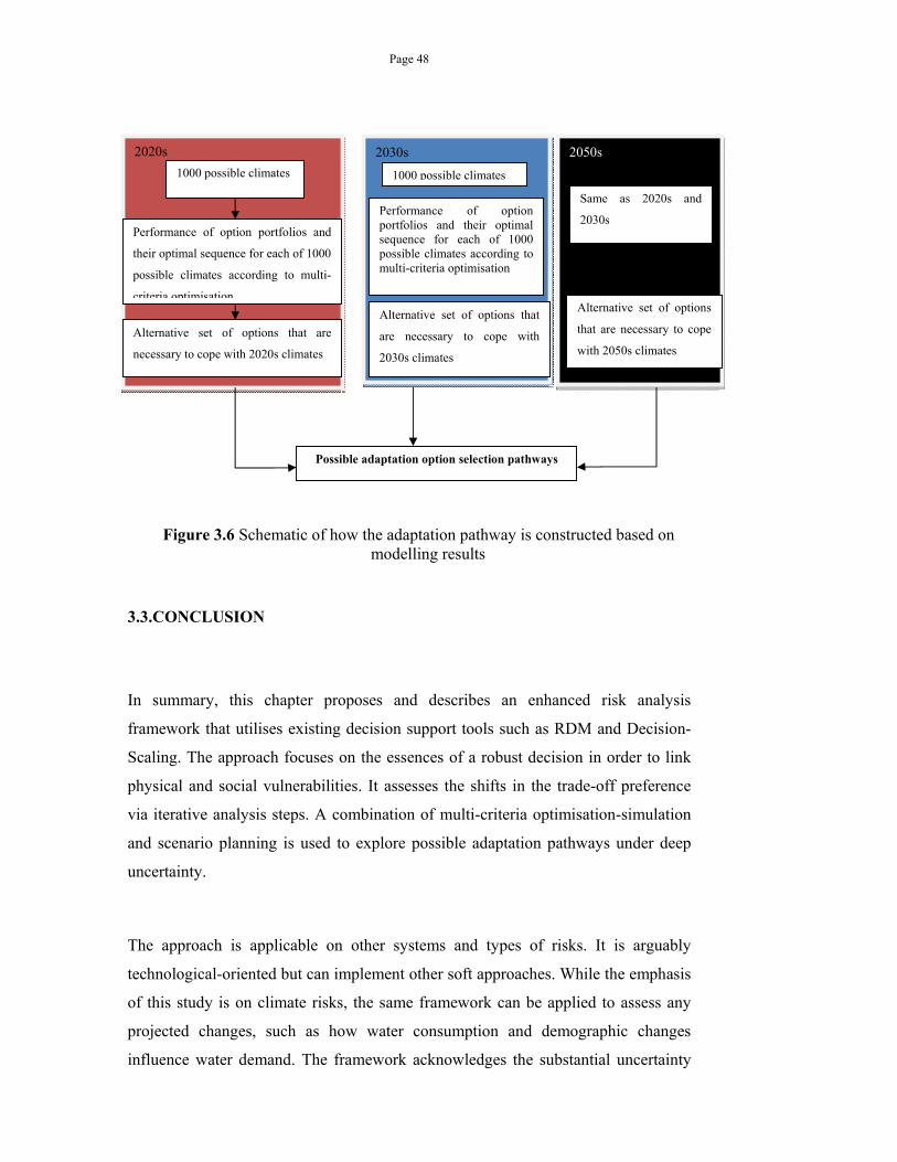
Page 48
Figure 3.6 Schematic of how the adaptation pathway is constructed based on modelling results
3.3.CONCLUSION
In summary, this chapter proposes and describes an enhanced risk analysis
framework that utilises existing decision support tools such as RDM and Decision-
Scaling. The approach focuses on the essences of a robust decision in order to link
physical and social vulnerabilities. It assesses the shifts in the trade-off preference
via iterative analysis steps. A combination of multi-criteria optimisation-simulation
and scenario planning is used to explore possible adaptation pathways under deep
uncertainty.
The approach is applicable on other systems and types of risks. It is arguably
technological-oriented but can implement other soft approaches. While the emphasis
of this study is on climate risks, the same framework can be applied to assess any
projected changes, such as how water consumption and demographic changes
influence water demand. The framework acknowledges the substantial uncertainty
S=3 available
options
2050s
2030s
Alternative set of options
that are necessary to cope
with 2050s climates
Alternative set of options that
are necessary to cope with
2030s climates
2020s
1000 possible climates
Performance of option portfolios and
their optimal sequence for each of 1000
possible climates according to multi-
criteria optimisation
Alternative set of options that are
necessary to cope with 2020s climates
Possible adaptation option selection pathways
Same as 2020s and
2030s Performance of option portfolios and their optimal sequence for each of 1000 possible climates according to multi-criteria optimisation
1000 possible climates

Page 49
from policy drivers. However, it is outside the scope of this study to deal explicitly
with this uncertainty factor. The framework does not deal with un-quantified risks,
but can potentially use qualitative risks as an extra context for analysing governance
and policy influences.
Page 50
Chapter 4. CASE STUDY DESCRIPTION
This chapter describes the chosen study area and how the methodology in Chapter 3
is applied to the case study. The study area is located in the southeast of England, an
area that has been susceptible to the past droughts of 1975-1976, 1995 and the recent
2010-2012 drought (Wigley and Atkinson, 1977; Hopkins, 1978; Marsh and Turton,
1996; Subak, 2000; Marsh et al., 2007; Kendon et al., 2013). Using a spatially
coherent stochastic model of monthly rainfall for the southeast, Duan et al. (2012)
has shown that some of these past droughts may recur in this region. Another study
also demonstrated that the region would require a net water supply increase of 441
Ml/day by 2035, 188 Ml/d of which due to potential climate change impacts (Water
Resources in the South East Group, 2010). Medd and Chappells (2007) further
asserted that such risk posed a key challenge in building resilience in water
management, since the current approach is fragmented and mainly employs
engineering measures to ensure supply. To highlight the main challenges in drought
planning and the requirements of adaptation decisions, Section 4.1 first describes
how water resource management in England and Wales operates; this description
helps identify the key decision makers and the major considerations of planning
decisions. This decision making process sets the scene for adaptation planning.
Based on analyses of the adaptation needs, Section 4.2 and 4.3 then explains how
the framework in Chapter 3 will be applied specifically for the study area, with
regard to climate uncertainty, hydrological uncertainty, demand uncertainty and
water resource uncertainty.
4.1.WATER RESOURCE MANAGEMENT IN ENGLAND AND WALES
Water management in England and Wales is a combination of private operation and
central regulation. On an operational level, the companies are privately owned and
largely responsible for their day-to-day business. On a planning level, water
4.1.1. A brief description
Page 51
companies are under the auspice of major regulating authorities: the Department for
Environment, Food and Rural Affairs (DEFRA), the Water Services Regulation
Authority (OFWAT) and the Environment Agency for England and Wales (EA)
(Arnell and Charlton, 2009). The EA and OFWAT evaluate the planning of the
water companies every five years via two planning reports (Southern Water, 2009b;
Southern Water, 2009a; Environment Agency, 2012). The first report is the water
resource management plan, which details how the companies will maintain a healthy
water supply-demand balance during the next 25 years. The second one, the business
plan, outlines how the companies will manage their revenue in the next five years.
Additionally the company annually reports its supply and financial performance,
along with an environmental impact assessment, to the Water Service Regulation
Authority. The business plan, the water resource management plan and monitoring
data are assessed in conjunction. In essence, the water resource management plan
details the need of infrastructure investments; this need then justifies the changes of
water price in the business plan. If the regulating authority does not approve the
proposed strategies in the water resource management plan, they can require the
company to either revise the plan or adjust the business plan accordingly. These
plans also form an important basis to assess the annual monitoring data, as the water
companies often use the demand projections in the water management plan as the
real demand in water shortage analysis.
Aside from these general planning documents, the companies have to consider other
risk-specific planning and relevant authorities. For instance, the Climate Change Act
2008 addresses climate change risks and the adaptation options (Planning & Climate
Change Coalition, 2010); the Flood and Water Management Act 2010 requires local
authorities to prepare flood risk management strategy and options to alter risks.
Drought wise, the company is required to maintain a Drought Contingency Plan,
which stipulates drought triggers and actions in the event of droughts. This plan does
not have a periodic review; it is amended every time the national policies are
revised. The Drought Plan and the Drought Direction 2011 also specifies several
types of emergency drought responses such as restrictions on water use and extra
supply options (Environment Agency, 2011). Water restrictions at the lowest level
are often termed as ‘hosepipe bans’ due to its restriction on 11 hosepipe-related uses.
Page 52
The Water Resources Act 1991, and later the Environment Act 1995 and the Water
Act 2003 set out three additional responses of water companies or Environment
Agency in the event of droughts (Department of Environment, 2011).
These three measures are described in Table 4-1 and include drought permit,
ordinary drought order and emergency drought order. Drought permits allow water
companies to take additional water from specified sources and place restriction on
their current sources. Ordinary drought orders let water companies restrict the non-
essential use of water while emergency drought orders, also termed ‘standpipes’,
further restrict water uses and let water companies provide water to the users via
standpipes or water tanks. The water companies use the frequency of these hosepipe
bans, such as 1 in 10 or 20 years, as a measure of their ‘level of service’. This level
of service is also mentioned in the corresponding water resource management plan,
as most water companies aim to maintain a certain level of service.
As such, water management in a water resource zone consists of four main actors,
three of them are: the water company that operates in the region, the environmental
regulator (the Environment Agency for England and Wales) and an economic
regulator (the Water Service Regulation Authority; Oftwat) (Arnell and Delaney,
2006; Sharp, 2006). The planning strategies are also subject to public consultation,
which engages the customers, arguably the fourth main actor. Figure 4.1
demonstrates the dynamics of decision making at such scale. The water company
interacts with the regulators regarding complying with legislation requirements,
preparing their long term plans as well as seeking approvals for drought responses.
Additionally neighbouring companies are also an important actor regarding water
transfer agreements. Furthermore, the company maintains relations with other
groups such as Natural England, river trusts, and other stakeholder groups.
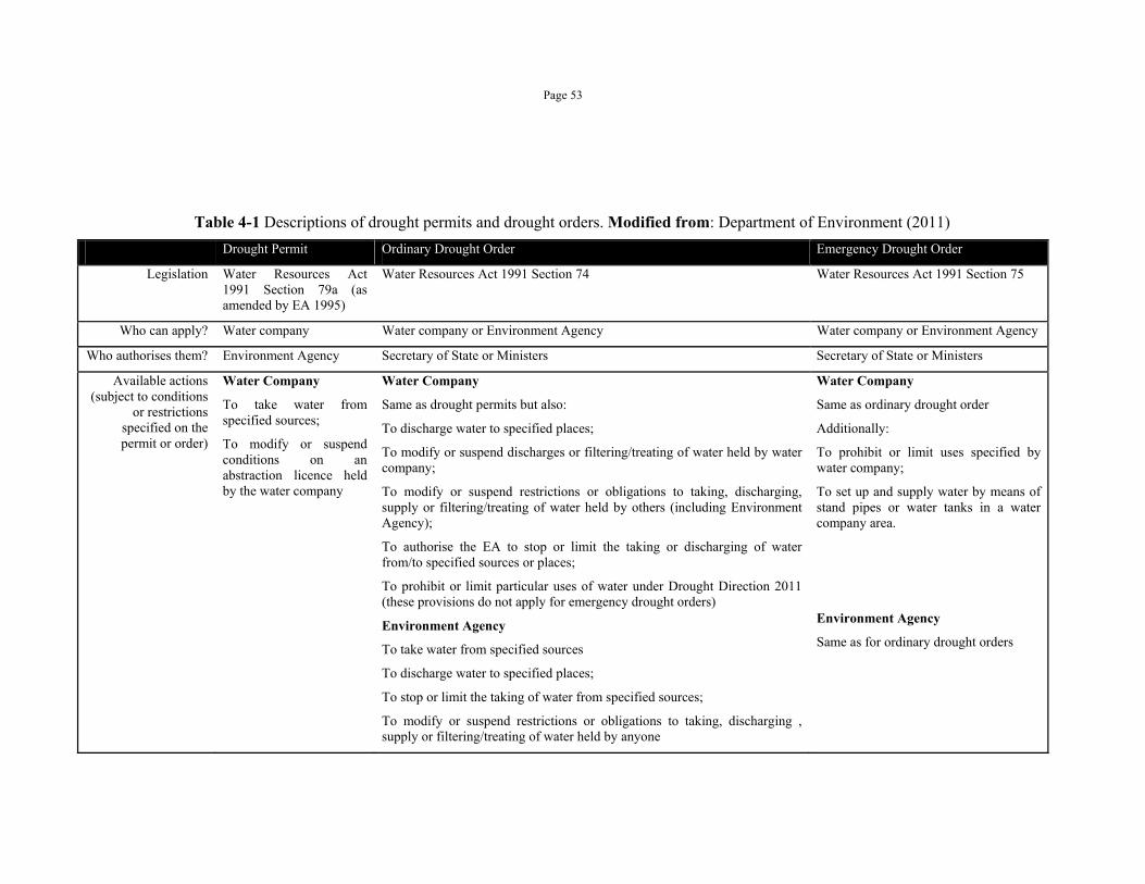
Page 53
Table 4-1 Descriptions of drought permits and drought orders. Modified from: Department of Environment (2011)
Drought Permit Ordinary Drought Order Emergency Drought Order
Legislation Water Resources Act 1991 Section 79a (as amended by EA 1995)
Water Resources Act 1991 Section 74 Water Resources Act 1991 Section 75
Who can apply? Water company Water company or Environment Agency Water company or Environment Agency
Who authorises them? Environment Agency Secretary of State or Ministers Secretary of State or Ministers
Available actions (subject to conditions
or restrictions specified on the permit or order)
Water Company
To take water from specified sources;
To modify or suspend conditions on an abstraction licence held by the water company
Water Company
Same as drought permits but also:
To discharge water to specified places;
To modify or suspend discharges or filtering/treating of water held by water company;
To modify or suspend restrictions or obligations to taking, discharging, supply or filtering/treating of water held by others (including Environment Agency);
To authorise the EA to stop or limit the taking or discharging of water from/to specified sources or places;
To prohibit or limit particular uses of water under Drought Direction 2011 (these provisions do not apply for emergency drought orders)
Environment Agency
To take water from specified sources
To discharge water to specified places;
To stop or limit the taking of water from specified sources;
To modify or suspend restrictions or obligations to taking, discharging , supply or filtering/treating of water held by anyone
Water Company
Same as ordinary drought order
Additionally:
To prohibit or limit uses specified by water company;
To set up and supply water by means of stand pipes or water tanks in a water company area.
Environment Agency
Same as for ordinary drought orders

Page 54
Figure 4.1 Water management framework in England and Wales
4.1.2. Planning decision cycles and decision variables
The structure of water management in England and Wales greatly affects the
decision making process of water companies (Cashman and Lewis, 2007). Overall, a
water company often focuses on strategic decisions proposed in the water resource
management and the business plan. There are two reasons for this focus: firstly,
most operational rules are determined at this level; secondly, regulators’ approvals
or objections at this level may determine the available planning options and the
implementation timeline, subsequently affect everyday operations and long-term
options. Indeed, the company controls and may vary its operations, but often follows
the strategies laid out in the two plans, particularly the short-term business plan.
As water companies are private but heavily regulated firms, their planning decisions
have to balance profit making and the quality of their water services (Helm and
Rajah, 1994; Ogden and Watson, 1999; Parker, 1999). While this balancing
requirement also exists for other industries, for the water industry the requirement is
implemented via the close supervision from the regulators (Saal and Parker, 2000).
This supervision ensures that the company does not abuse its position to make profit
at the expenses of the customers and the environment. Often, a private firm can
make money via selling a sufficient number of products and/or setting the price
higher than the cost. Since the water companies operate on water, a limited resource,
Cost-Benefit and Risk analysis
OFWAT-Financial and Performance
Regulator
Environment Agency for
England and Wales-
Environment Regulator
Water company Neighbour companies Water customers
Strategic Operational
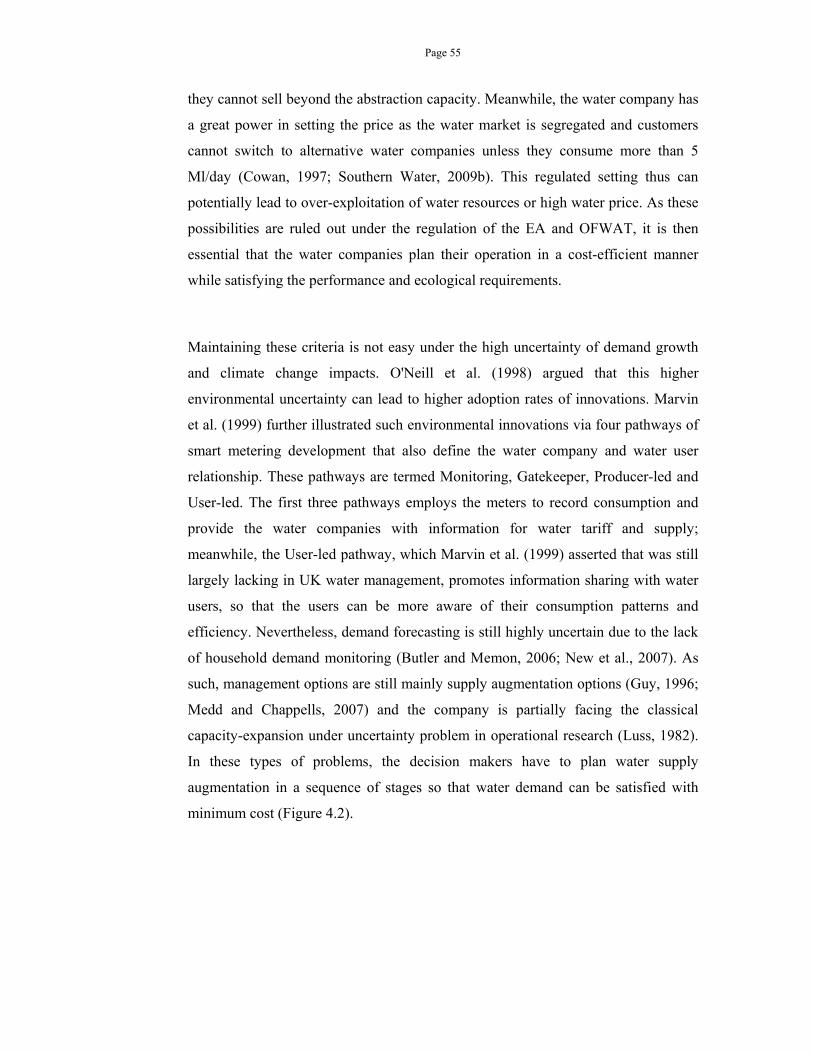
Page 55
they cannot sell beyond the abstraction capacity. Meanwhile, the water company has
a great power in setting the price as the water market is segregated and customers
cannot switch to alternative water companies unless they consume more than 5
Ml/day (Cowan, 1997; Southern Water, 2009b). This regulated setting thus can
potentially lead to over-exploitation of water resources or high water price. As these
possibilities are ruled out under the regulation of the EA and OFWAT, it is then
essential that the water companies plan their operation in a cost-efficient manner
while satisfying the performance and ecological requirements.
Maintaining these criteria is not easy under the high uncertainty of demand growth
and climate change impacts. O'Neill et al. (1998) argued that this higher
environmental uncertainty can lead to higher adoption rates of innovations. Marvin
et al. (1999) further illustrated such environmental innovations via four pathways of
smart metering development that also define the water company and water user
relationship. These pathways are termed Monitoring, Gatekeeper, Producer-led and
User-led. The first three pathways employs the meters to record consumption and
provide the water companies with information for water tariff and supply;
meanwhile, the User-led pathway, which Marvin et al. (1999) asserted that was still
largely lacking in UK water management, promotes information sharing with water
users, so that the users can be more aware of their consumption patterns and
efficiency. Nevertheless, demand forecasting is still highly uncertain due to the lack
of household demand monitoring (Butler and Memon, 2006; New et al., 2007). As
such, management options are still mainly supply augmentation options (Guy, 1996;
Medd and Chappells, 2007) and the company is partially facing the classical
capacity-expansion under uncertainty problem in operational research (Luss, 1982).
In these types of problems, the decision makers have to plan water supply
augmentation in a sequence of stages so that water demand can be satisfied with
minimum cost (Figure 4.2).
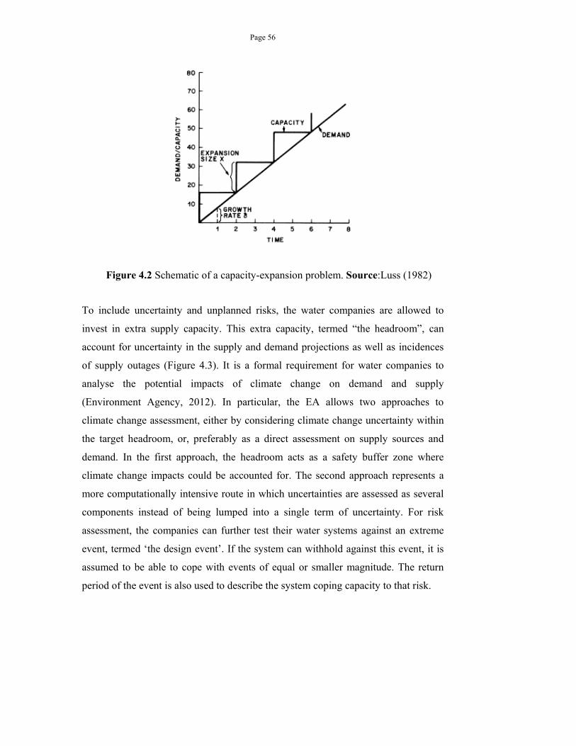
Page 56
Figure 4.2 Schematic of a capacity-expansion problem. Source:Luss (1982)
To include uncertainty and unplanned risks, the water companies are allowed to
invest in extra supply capacity. This extra capacity, termed “the headroom”, can
account for uncertainty in the supply and demand projections as well as incidences
of supply outages (Figure 4.3). It is a formal requirement for water companies to
analyse the potential impacts of climate change on demand and supply
(Environment Agency, 2012). In particular, the EA allows two approaches to
climate change assessment, either by considering climate change uncertainty within
the target headroom, or, preferably as a direct assessment on supply sources and
demand. In the first approach, the headroom acts as a safety buffer zone where
climate change impacts could be accounted for. The second approach represents a
more computationally intensive route in which uncertainties are assessed as several
components instead of being lumped into a single term of uncertainty. For risk
assessment, the companies can further test their water systems against an extreme
event, termed ‘the design event’. If the system can withhold against this event, it is
assumed to be able to cope with events of equal or smaller magnitude. The return
period of the event is also used to describe the system coping capacity to that risk.
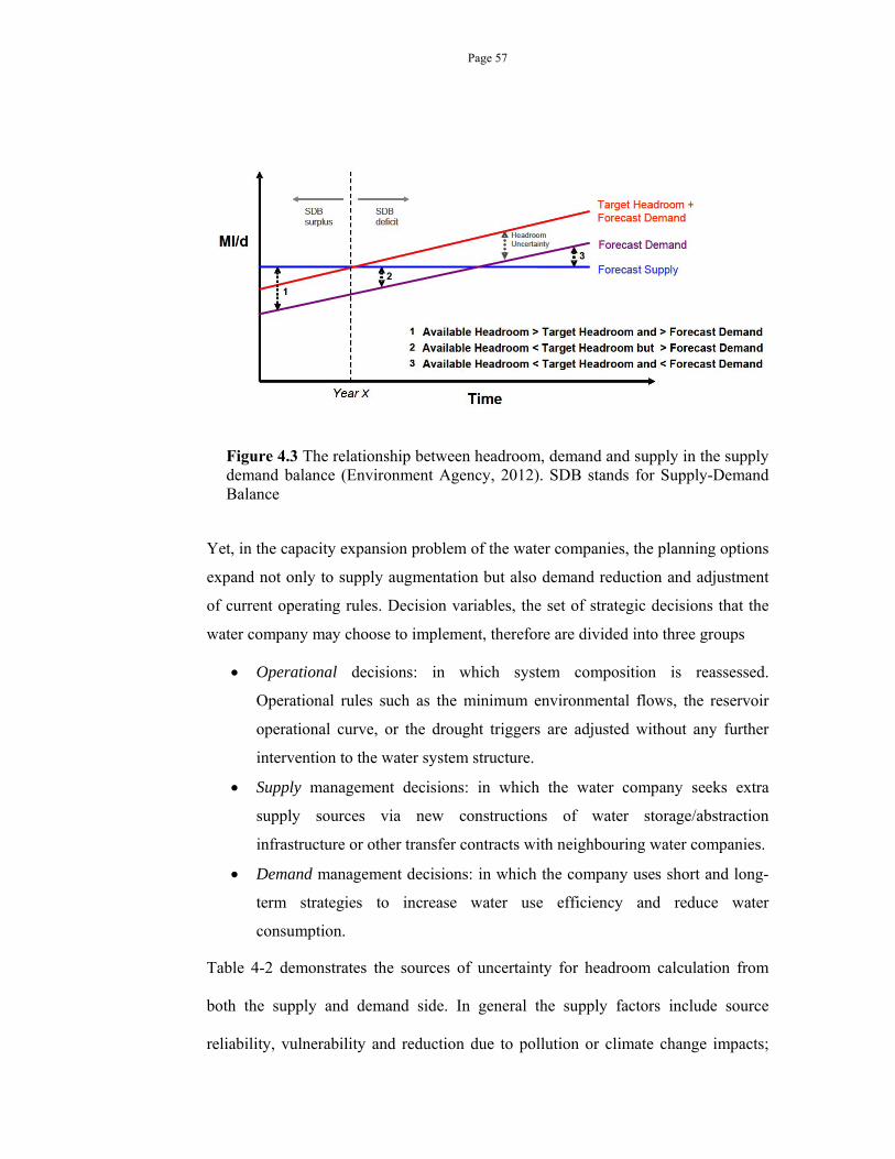
Page 57
Figure 4.3 The relationship between headroom, demand and supply in the supply demand balance (Environment Agency, 2012). SDB stands for Supply-Demand Balance
Yet, in the capacity expansion problem of the water companies, the planning options
expand not only to supply augmentation but also demand reduction and adjustment
of current operating rules. Decision variables, the set of strategic decisions that the
water company may choose to implement, therefore are divided into three groups
Operational decisions: in which system composition is reassessed.
Operational rules such as the minimum environmental flows, the reservoir
operational curve, or the drought triggers are adjusted without any further
intervention to the water system structure.
Supply management decisions: in which the water company seeks extra
supply sources via new constructions of water storage/abstraction
infrastructure or other transfer contracts with neighbouring water companies.
Demand management decisions: in which the company uses short and long-
term strategies to increase water use efficiency and reduce water
consumption.
Table 4-2 demonstrates the sources of uncertainty for headroom calculation from
both the supply and demand side. In general the supply factors include source
reliability, vulnerability and reduction due to pollution or climate change impacts;
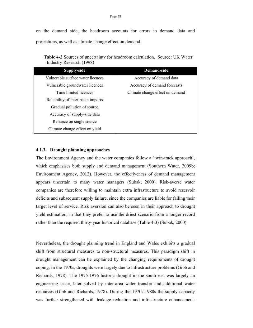
Page 58
on the demand side, the headroom accounts for errors in demand data and
projections, as well as climate change effect on demand.
Table 4-2 Sources of uncertainty for headroom calculation. Source: UK Water Industry Research (1998)
Supply-side Demand-side
Vulnerable surface water licences
Vulnerable groundwater licences
Time limited licences
Reliability of inter-basin imports
Gradual pollution of source
Accuracy of supply-side data
Reliance on single source
Climate change effect on yield
Accuracy of demand data
Accuracy of demand forecasts
Climate change effect on demand
4.1.3. Drought planning approaches
The Environment Agency and the water companies follow a ‘twin-track approach’,
which emphasises both supply and demand management (Southern Water, 2009b;
Environment Agency, 2012). However, the effectiveness of demand management
appears uncertain to many water managers (Subak, 2000). Risk-averse water
companies are therefore willing to maintain extra infrastructure to avoid reservoir
deficits and subsequent supply failure, since the companies are liable for failing their
target level of service. Risk aversion can also be seen in their approach to drought
yield estimation, in that they prefer to use the driest scenario from a longer record
rather than the required thirty-year historical database (Table 4-3) (Subak, 2000).
Nevertheless, the drought planning trend in England and Wales exhibits a gradual
shift from structural measures to non-structural measures. This paradigm shift in
drought management can be explained by the changing requirements of drought
coping. In the 1970s, droughts were largely due to infrastructure problems (Gibb and
Richards, 1978). The 1975-1976 historic drought in the south-east was largely an
engineering issue, later solved by inter-area water transfer and additional water
resources (Gibb and Richards, 1978). During the 1970s-1980s the supply capacity
was further strengthened with leakage reduction and infrastructure enhancement.
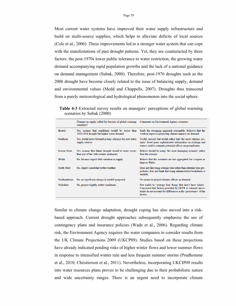
Page 59
Most current water systems have improved their water supply infrastructure and
build on multi-source supplies, which helps to alleviate deficits of local sources
(Cole et al., 2006). These improvements led to a stronger water system that can cope
with the manifestations of past drought patterns. Yet, they are counteracted by three
factors: the post-1970s lower public tolerance to water restriction, the growing water
demand accompanying rapid population growths and the lack of a national guidance
on demand management (Subak, 2000). Therefore, post-1976 droughts such as the
2006 drought have become closely related to the issue of balancing supply, demand
and environmental values (Medd and Chappells, 2007). Droughts thus transcend
from a purely meteorological and hydrological phenomenon into the social sphere.
Table 4-3 Extracted survey results on managers’ perceptions of global warming scenarios by Subak (2000)
Similar to climate change adaptation, drought coping has also moved into a risk-
based approach. Current drought approaches subsequently emphasise the use of
contingency plans and insurance policies (Wade et al., 2006). Regarding climate
risk, the Environment Agency requires the water companies to consider results from
the UK Climate Projections 2009 (UKCP09). Studies based on these projections
have already indicated pending risks of higher winter flows and lower summer flows
in response to intensified winter rain and less frequent summer storms (Prudhomme
et al., 2010; Christierson et al., 2011). Nevertheless, incorporating UKCIP09 results
into water resources plans proves to be challenging due to their probabilistic nature
and wide uncertainty ranges. There is an urgent need to incorporate climate
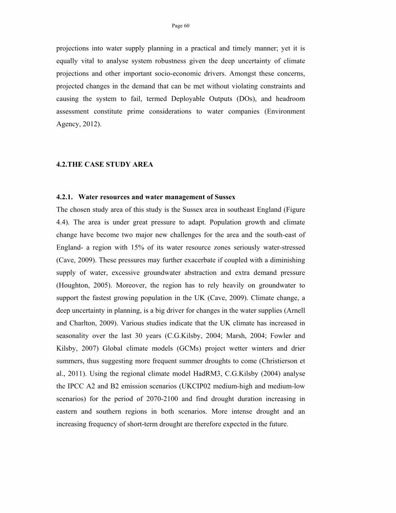
Page 60
projections into water supply planning in a practical and timely manner; yet it is
equally vital to analyse system robustness given the deep uncertainty of climate
projections and other important socio-economic drivers. Amongst these concerns,
projected changes in the demand that can be met without violating constraints and
causing the system to fail, termed Deployable Outputs (DOs), and headroom
assessment constitute prime considerations to water companies (Environment
Agency, 2012).
4.2.THE CASE STUDY AREA
4.2.1. Water resources and water management of Sussex
The chosen study area of this study is the Sussex area in southeast England (Figure
4.4). The area is under great pressure to adapt. Population growth and climate
change have become two major new challenges for the area and the south-east of
England- a region with 15% of its water resource zones seriously water-stressed
(Cave, 2009). These pressures may further exacerbate if coupled with a diminishing
supply of water, excessive groundwater abstraction and extra demand pressure
(Houghton, 2005). Moreover, the region has to rely heavily on groundwater to
support the fastest growing population in the UK (Cave, 2009). Climate change, a
deep uncertainty in planning, is a big driver for changes in the water supplies (Arnell
and Charlton, 2009). Various studies indicate that the UK climate has increased in
seasonality over the last 30 years (C.G.Kilsby, 2004; Marsh, 2004; Fowler and
Kilsby, 2007) Global climate models (GCMs) project wetter winters and drier
summers, thus suggesting more frequent summer droughts to come (Christierson et
al., 2011). Using the regional climate model HadRM3, C.G.Kilsby (2004) analyse
the IPCC A2 and B2 emission scenarios (UKCIP02 medium-high and medium-low
scenarios) for the period of 2070-2100 and find drought duration increasing in
eastern and southern regions in both scenarios. More intense drought and an
increasing frequency of short-term drought are therefore expected in the future.
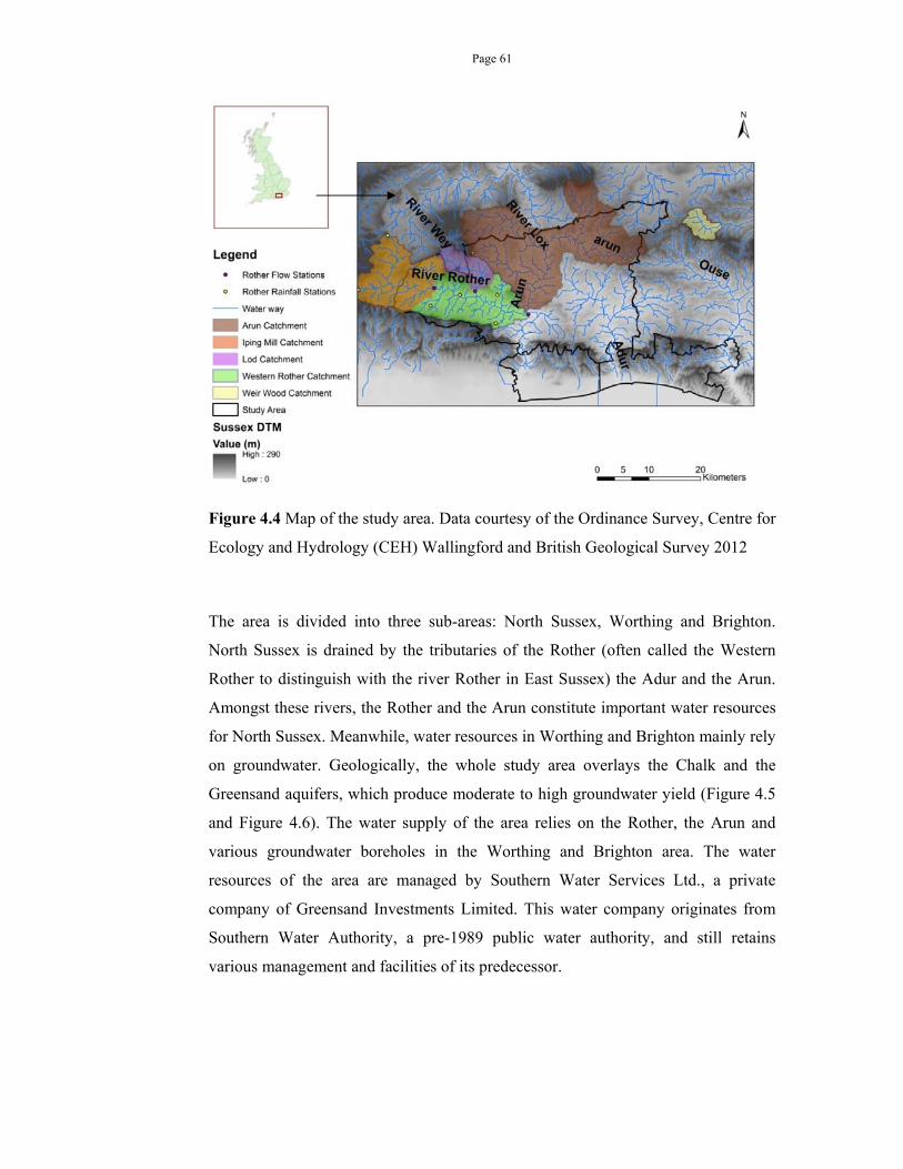
Page 61
Figure 4.4 Map of the study area. Data courtesy of the Ordinance Survey, Centre for
Ecology and Hydrology (CEH) Wallingford and British Geological Survey 2012
The area is divided into three sub-areas: North Sussex, Worthing and Brighton.
North Sussex is drained by the tributaries of the Rother (often called the Western
Rother to distinguish with the river Rother in East Sussex) the Adur and the Arun.
Amongst these rivers, the Rother and the Arun constitute important water resources
for North Sussex. Meanwhile, water resources in Worthing and Brighton mainly rely
on groundwater. Geologically, the whole study area overlays the Chalk and the
Greensand aquifers, which produce moderate to high groundwater yield (Figure 4.5
and Figure 4.6). The water supply of the area relies on the Rother, the Arun and
various groundwater boreholes in the Worthing and Brighton area. The water
resources of the area are managed by Southern Water Services Ltd., a private
company of Greensand Investments Limited. This water company originates from
Southern Water Authority, a pre-1989 public water authority, and still retains
various management and facilities of its predecessor.
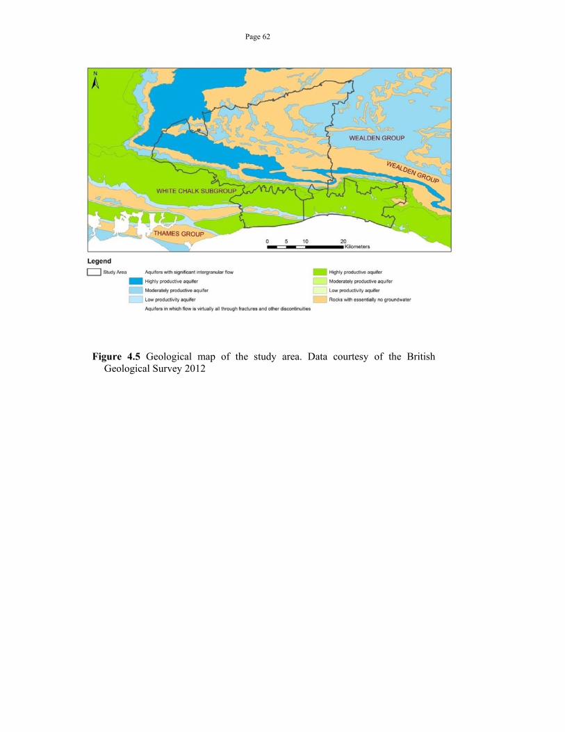
Page 62
Figure 4.5 Geological map of the study area. Data courtesy of the British Geological Survey 2012
Page 63
Figure 4.6 Groundwater abstraction map of the study area. Source: British Geological Survey
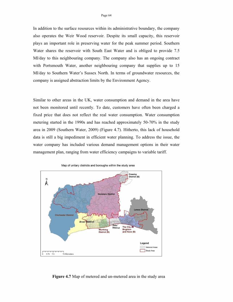
Page 64
In addition to the surface resources within its administrative boundary, the company
also operates the Weir Wood reservoir. Despite its small capacity, this reservoir
plays an important role in preserving water for the peak summer period. Southern
Water shares the reservoir with South East Water and is obliged to provide 7.5
Ml/day to this neighbouring company. The company also has an ongoing contract
with Portsmouth Water, another neighbouring company that supplies up to 15
Ml/day to Southern Water’s Sussex North. In terms of groundwater resources, the
company is assigned abstraction limits by the Environment Agency.
Similar to other areas in the UK, water consumption and demand in the area have
not been monitored until recently. To date, customers have often been charged a
fixed price that does not reflect the real water consumption. Water consumption
metering started in the 1990s and has reached approximately 50-70% in the study
area in 2009 (Southern Water, 2009) (Figure 4.7). Hitherto, this lack of household
data is still a big impediment in efficient water planning. To address the issue, the
water company has included various demand management options in their water
management plan, ranging from water efficiency campaigns to variable tariff.
Figure 4.7 Map of metered and un-metered area in the study area
Page 65
From a planning decision perspective, the company plans its strategies, also viewed
as decision variables in decision analysis, via the water resource plans. Its reservoirs
operate based on control curves, which dictate when water is stored or released.
These control curves are reviewed at the same time as the production plans. For
groundwater, as it is difficult to project groundwater sources at the moment, the
sustainable available groundwater abstraction is determined as the amount available
under the worst drought during 1920 to 1921 in Kent. Operational rules are reviewed
as follows:
Monthly for normal period
If there are impending droughts: fortnightly review
Once drought starts: weekly review
In extreme droughts: daily
For strategic planning, there are the Drought Plan and Water Resource Management
Plan. The Water Resource Management Plan makes long-term decisions that
maintain the targeted level of service. During the drought period, as described in
Section 4.1, response actions could include hosepipe bans, non-essential bans and
standpipe.
4.2.2. Main requirements of adaptation: perspectives of the decision makers
Several meetings have been held between Southern Water and the researcher to
clarify view points and address adaptation needs. The company recognises droughts
as a serious risk in the study area and targets this issue in their adaptation planning.
The EA made clear in their Water Resource Guideline (Environment Agency, 2012)
that robustness and reliability are key criteria in assessing the water resource
systems. The current approach of Southern Water emphasises a resilient and flexible
water resource system, based on information and modelling work accumulated from
the previous planning cycles. In addressing robustness, the company aims that their
options are not only tested against historical droughts but also on synthetic events
based on past droughts. In terms of resilience, it tries to maintain the targeted level
of service of 1-in-10-year hosepipe ban against the severity of the worst historic
drought 1921-1922. The company viewed a resilient option as an option that can
accommodate droughts up to the design drought event. In its definitions, there is a
Page 66
significant overlap between the concept of robustness and resilience. Its approach is
strongly risk and frequency-based. It specifically analyses the level of service in
conjunction with the Deployable Output, the maximum supply that does not damage
the water sources and the environment. Via this analysis, the company can assess the
maximum sustainable level of Deployable Output that does not affect the sources
and worsen the targeted level of service. The company also highlighted the
importance of an outage plan, since supply outages in stressed periods might have a
significant impact. Compound risks are also a vital factor. For instance, a
combination of groundwater droughts and sudden flash floods can severely affect
water supply, as the groundwater sources are depleted and the surface water requires
substantial turbidity treatment. While maintaining the use of hosepipe bans and the
Drought Plan, the company tries to not rely on drought permits, or in other words
achieving robustness based on permits, as frequent applications for permits are
penalised by the EA. Furthermore, the average time to obtain a drought permit is
three months and thus it is highly uncertain whether that permit is still needed once
granted.
In terms of demand management, the water company has attempted to apply data
mining techniques, such as Artificial Neural Network, to analyse demand patterns.
This approach is limited by data availability, since most available demand data is at
a macro scale (bulk consumption) and the current available approach is micro-
component based. Nevertheless, the company gradually possesses more data on
demand patterns and behaviour with roughly ten years of data since metering started
in 2000. The current measuring regime, however, reads the meters every six months
(and not on the same day for the whole area). Due to this lack of daily household
demand data, the company has introduced smart meters which will facilitate more
advanced demand modelling. Even so, research based on smart metering data is only
feasible after three to four years when sufficient data have been accumulated. To
date, most of the work yields limited forecasting power; demand projections are
instead based on assumptions on per-capita consumption, the number of households
and demographic trends. Similar to supply analysis, the company is using
deterministic demand models but aims to shift to stochastic models. The company
also remains cautious in demand option analysis, as water efficiency might have
Page 67
been brought down by stealth water efficiency (more efficient white good such as
dishwasher and washing machine) and the effect of seasonal tariff is still uncertain.
4.3.APPLICATION OF THE FRAMEWORK
The Sussex area is suitable for a case study because: the decision makers advocate
the concept of robustness and resilience; they specify key requirements of their
adaptation decision; and relevant data are available for the region. The study thus
applies the conceptual framework described in Chapter 3 based on minimising
operational cost, supply deficit and environmental flow deficits, the three criteria
identified by the decision makers. As the company emphasises the need for robust,
resilient and flexible drought planning, the robust decision making framework has
been designed to consider the key uncertainties in climate projections and
hydrological modelling, while addressing changing water demand. The aim of
applying the framework on the case study was to tackle the uncertainty cascade and
address the adaptation needs of the decision makers.
This section outlines the data to be used in the framework. More details on the data
and how they are used in each analysis component will be provided in the
corresponding chapters. The framework, as presented in Chapter 3, addresses
climate, hydrological and demand uncertainty and linked by the water resource-
decision analysis model. Each component of the whole framework is outlined as
follows
4.3.1. Climate uncertainty
The chosen climate projections for the study area are based on the results of the
Hadley Centre Regional Climate Model HadRM3 climate model (hereby also
termed the RCM in general), a regional climate model of the Hadley Centre
produced by the UK Meteorological Office. The chosen emission scenario is the
Medium Emission Scenario. The model outputs exist in several forms, such as
10,000 Change Factors of the 2009 UK Climate Projections (UKCP09), the original
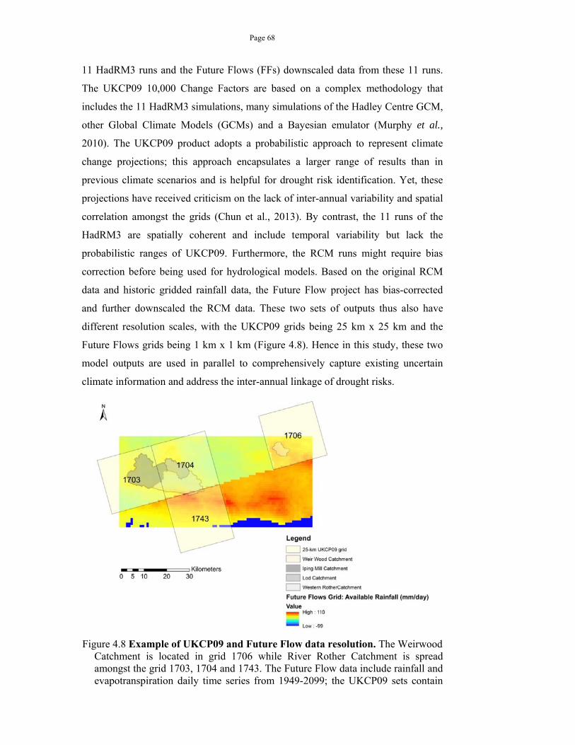
Page 68
11 HadRM3 runs and the Future Flows (FFs) downscaled data from these 11 runs.
The UKCP09 10,000 Change Factors are based on a complex methodology that
includes the 11 HadRM3 simulations, many simulations of the Hadley Centre GCM,
other Global Climate Models (GCMs) and a Bayesian emulator (Murphy et al.,
2010). The UKCP09 product adopts a probabilistic approach to represent climate
change projections; this approach encapsulates a larger range of results than in
previous climate scenarios and is helpful for drought risk identification. Yet, these
projections have received criticism on the lack of inter-annual variability and spatial
correlation amongst the grids (Chun et al., 2013). By contrast, the 11 runs of the
HadRM3 are spatially coherent and include temporal variability but lack the
probabilistic ranges of UKCP09. Furthermore, the RCM runs might require bias
correction before being used for hydrological models. Based on the original RCM
data and historic gridded rainfall data, the Future Flow project has bias-corrected
and further downscaled the RCM data. These two sets of outputs thus also have
different resolution scales, with the UKCP09 grids being 25 km x 25 km and the
Future Flows grids being 1 km x 1 km (Figure 4.8). Hence in this study, these two
model outputs are used in parallel to comprehensively capture existing uncertain
climate information and address the inter-annual linkage of drought risks.
Figure 4.8 Example of UKCP09 and Future Flow data resolution. The Weirwood Catchment is located in grid 1706 while River Rother Catchment is spread amongst the grid 1703, 1704 and 1743. The Future Flow data include rainfall and evapotranspiration daily time series from 1949-2099; the UKCP09 sets contain
Page 69
the mean change factors that can be applied on the historic 1961-1990 baseline time series to present future tri-decadal, such as the 2020s, 2030s and the 2050s. The future flow rainfall presented in this figure is the axfq0 RCM (1 of the 11 runs) run for the 1st November 2099.
4.3.2. Hydrological data and model
The hydrological model used in this study is the Catchment Model (CATCHMOD),
a hydrological model used by the Environment Agency and several water
companies. The model uses rainfall and evapotranspiration (PET) inputs to simulate
surface, subsurface flows and groundwater level. The model represents a catchment
as one reservoir, parameters of which present geology, land use and drainage
characteristics of the catchment. The water company has been using the model in
various submissions of its water management plan. During previous preparation
work for the water management plans, the parameters of the model have been
calibrated and validated based on the 1990-2005 historic flows of the river Rother
and the Weir Wood Reservoir. The calibration period was the 1990-1999 period and
the validation period was the 2000-2004 period. In this study, these sets of
parameters are used along with recalibration using other periods and calibration
criteria. This comparison explores structural uncertainty and parameter uncertainty
of the hydrological component.
4.3.3. Demand modelling
In the demand modelling component, the demand projections of Southern Water for
2020s and 2030s are used. For 2050s, the study uses the four EA socio-economic
demand scenarios, which project water demand based on different governance and
societal structures (Environment Agency, 2008). More details about the demand
scenarios will be provided in Chapter 7. Of these scenarios, the Uncontrolled
Demand is the most severe scenario that includes substantial population growth and
increasing water consumption. In other scenarios, water demand grows or slightly
reduces due to innovation in technology and reduced water consumption per capita.
The Southern Water and the EA water demand projections were scaled from the
1995 demand profile using a scaling factor, the ratio between the annual average
demand of the projected period and the annual average demand of 1995. This
scaling process thus preserves the daily pattern of the demand fluctuation and
mimics demand changes over the year.
Page 70
4.3.4. Water resource modelling and option analysis
In the current practice of Southern Water, water resource modelling and option
appraisal are separate. The water resource modelling software the company uses,
Aquator, is a water resource model that can simulate and optimise the water supply-
demand balance at a daily time step. At the current setting, the model is mostly run
in the simulation mode, with optimisation being applied to certain bi-directional
links of the network. The Sussex Aquator model presents the water system as a
network of links and nodes. Groundwater supply is fixed and based on the EA’s
abstraction licences. Surface water, however, is varied and based on CATCHMOD
outputs of Rother and Weir Wood flows. The whole 1888-2005 time series, which
include the severe 1921-1922 and 1975-1976 droughts, are used to test the system
performance. Meanwhile, option appraisal is analysed in a separate optimisation
model that selects options based on their average Deployable Output, investment
cost and operational cost.
In this study, the water resource modelling and option appraisal model are
combined. This combination integrates the financial investment and performance
indicator. Without this integration, option appraisal was based on the expected cost
and utility, calculated as
∗ ∗
Equation 4-1
With Coption being the total cost of the option
foption being the frequency of usages
U being the utility, such as the Deployable Output and E(U) is the expected
utility
coption being the cost per unit
By contrast, if the two models are integrated, cost analysis can better reflect option
cost and based on the real utility, such that
Page 71
∗
Equation 4-2
With T being the total simulation time
The latter method thus reduces the uncertainty of using the average utility and
frequency of usages. Combining the two models will help reduce the analysis effort
as climate projections include a large number of cases. The UKCP09 projections
consists of 10,000 realisations for each time period; assessing the average frequency
and usage for each cases will create 10,000 runs for water resource analysis and
10,000 option appraisals. In comparison, a nested approach readily analyses the
options within the runs of water resource analysis and thus eliminate the separate
option appraisal runs. Thirdly, this setting can further facilitate changes in criteria
preferences of the decision makers, such as using average water deficit instead of the
most severe water deficit. When the two models are separated, this change in
references would require re-running the water resource model and the option
appraisal model. Meanwhile, the integrated model requires only one rerun of the
integrated model.
4.3.5. Robust decision analysis
The previous components allow detailed analysis of data uncertainty in climate
modelling, parameter uncertainty in hydrological modelling, and model uncertainty
in demand projection and water resource modelling. Robust Decision Analysis, in
line with the description in Chapter 3, links these components for a comprehensive
analysis. In response to Southern Water’s point on the outage plan, the framework
also includes outage testing, in which supply sources are taken out or reduced to test
system resilience.
All the components, as the contributing factors of the water resource assessment, are
linked. The uncertainty identified in each component is also cascaded into relevant
components, so that their overall contribution can be analysed. The climate
uncertainty component is linked with the hydrological component, thus the
uncertainty in the hydrological outputs will consists of climate uncertainty and
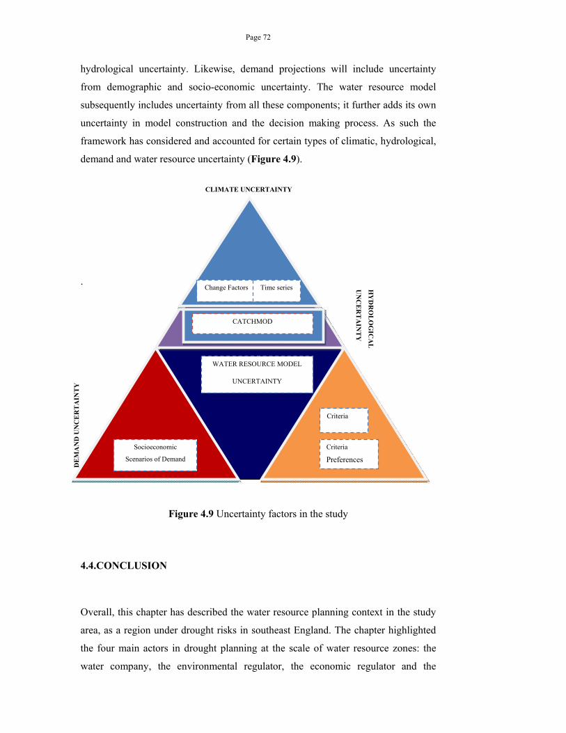
Page 72
hydrological uncertainty. Likewise, demand projections will include uncertainty
from demographic and socio-economic uncertainty. The water resource model
subsequently includes uncertainty from all these components; it further adds its own
uncertainty in model construction and the decision making process. As such the
framework has considered and accounted for certain types of climatic, hydrological,
demand and water resource uncertainty (Figure 4.9).
.
Figure 4.9 Uncertainty factors in the study
4.4.CONCLUSION
Overall, this chapter has described the water resource planning context in the study
area, as a region under drought risks in southeast England. The chapter highlighted
the four main actors in drought planning at the scale of water resource zones: the
water company, the environmental regulator, the economic regulator and the
HY
DR
OL
OG
ICA
L
UN
CE
RT
AIN
TY
CLIMATE UNCERTAINTY
DE
MA
ND
UN
CE
RT
AIN
TY
Change Factors Time series
CATCHMOD
Socioeconomic
Scenarios of Demand
Criteria
Criteria
Preferences
WATER RESOURCE MODEL
UNCERTAINTY
Page 73
customers. Main challenges in drought planning including robust planning amidst
uncertainty, balancing between profit making and environmental services and
constructing adaptation pathways given the drought risks. The chapter has also
outlined the uncertainty factors to be analysed in the next chapters. In essence,
Chapter 5 will focus on climate uncertainty, Chapter 6 on hydrological uncertainty,
Chapter 7 on vulnerability of the Sussex water resource system, Chapter 8 on
planning options and Chapter 9 on an integrated analysis of robust planning. The
chapter also described the study area and its key requirements in adaptation. The
area is divided into three water resource zones, all of which are dependent on
groundwater. Amongst these three areas, the Sussex North has major surface water
sources from the River Rother and the Weirwood Reservoir. The decision makers in
the case study have identified the need to adopt robust and resilient water resource
planning. Based on the adaptation requirements, the Robust Decision Analysis
framework in Chapter 3 has been adapted to consider climate uncertainty,
hydrological uncertainty, socio-economic uncertainty and water resource
uncertainty.
Page 74
Chapter 5. CLIMATE UNCERTAINTY
5.1.INTRODUCTION
The south-east of England has been subject to severe droughts in the past and still
remains vulnerable in the future. Droughts, as a natural phenomenon, have
cascading impacts on the water resources, the ecosystem and the socio-economic
system (Dracup et al., 1980; Wilhite and Glantz, 1985; McKee et al., 1993). As a
meteorological phenomenon, droughts are signified by precipitation deficiency over
an extended period (McMahon and Arenas, 1982). This temporary deficiency may
affect water supply for crops and river flows, thus can also manifest as agricultural
and hydrological droughts. As droughts do not have a clear onset and ending
symptom, it is difficult to identify droughts. Drought types are hence often
recognised based on their impacts; classified into meteorological, agricultural and
hydrological droughts (Dai, 2011). Traditionally, droughts are assumed to first
appear as a meteorological event, when the precipitation does not meet the normal
atmospheric balance. These conditions can dry up the soil (soil moisture droughts),
lead to plant stress (agricultural droughts) and river flow deficiency (hydrological
droughts). The impacts subsequently disrupt the normal operation of the economy
and water management, leading to the corresponding drought types. However, with
the current changing climate and increased natural climate variability (Arnell,
1999b), drought impacts might occur simultaneously, affecting the most vulnerable
system and not in the expected order of meteorological, hydrological and
agricultural droughts. As such, drought planning requires information on how the
risk arises, what the impending changes are, particularly with regard to changes in
climate and local water demand.
Yet, climate change projections are plagued with uncertainty. Uncertainty not only
represents our incomplete knowledge of the climate system, but also characterizes
Page 75
the dynamic Earth system. As climate change assessments involve a chain of general
circulation models (GCMs), regional climate models (RCMs) to impact models, the
uncertainty is set to propagate. The impacts of uncertainty in climate projections can
well be traced in drought prospects (Burke and Brown, 2010; Rahiz and New, 2013),
subsequent flow projections (Wilby, 2005; Feyen and Dankers, 2009), crop yields
(Lobell et al., 2008) and water availability (Fowler et al., 2007; Wade et al., 2013).
On a local scale, the added uncertainty may arise from the downscaling process,
which adjusts the raw projections to better characterize the local climate (Chen et
al., 2011). That wide range of uncertainty further expands when several alternative
climate projections are considered. However, many assessments often focus on one
climate data source.
The term “climate post-processing” is often used to refer to the process of bias
correction or downscaling (Vannitsem, 2011; Imbery et al., 2013). In this study, it is
expanded to all general process of converting climate model outputs into products
and information of different formats, variables and temporal/spatial scales. To date,
studies have demonstrated that post-processing of climate model outputs can adjust
the flood risk represented by the final product. For instance, Cloke et al. (2012) have
shown that certain post-processing of UKCP09 RCMs can increase uncertainty and
further modify the modelled flood risks of the Upper Severn, UK. Kay and Jones
(2012) showed relatively consistent median changes in flood frequency amongst the
UKCP09 change factors, the Weather Generator, and the UKCP09 RCMs data;
nevertheless, due to the data format and the perturbation method, the change factor
format leads to less variability than the time series format of the same climate
information.
These discrepancies may exist beyond projections of flood risk. As a recurring
climate risk, droughts are also subject to the changes indicated in climate projections
(Marsh, 2007). While climate information points toward increasing drought risks in
the future, they show varying degrees of changes that may be indicative of structural
uncertainty and post-processing uncertainty. In particular, the multi-model RCMs of
the PRUDENCE project show an increase of short-term summer droughts and lower
Page 76
risks of prolonged severe droughts, albeit with high uncertainty due to the RCMs’
poor skills in simulating severe events and other uncertainty cascaded from the
driving GCM (Blenkinsop and Fowler, 2007). Using the RCM HadRM3 data from
the UK Meteorological Office, Burke and Brown (2010) could recreate observed
drought events but found that for the 1959-2002 period the model slightly
overestimates drought area while underestimate drought frequency and severity.
Meanwhile, the 1960-2080 UKCP09 data project a lowering mean daily river flows
for all months in the Medway catchment and with climate signals dominating the
hydrological uncertainty (Cloke et al., 2010b). Finally, using the UKCP09 change
factors, (Christierson et al., 2011) show a high likelihood of declining summer flows
in 70 UK-wide catchments in the 2020s with the main uncertainty coming from the
spread in climate projections. These projected reductions and their variation across
climate data sources are critical for water resources planning as they may lead to
different adaptation plans and implementation schedules. As a potential source of
uncertainty, there is a need to examine the post-processing uncertainty in climate
products, particularly for those of the same source but having undergone different
post-processing methods.
As described in Chapter 1, the focus of this thesis is on water resources drought,
defined as a precipitation deficit to the normal functioning of the water system. A
comprehensive analysis of water resources drought requires a conjunctive
assessment of meteorological, hydrological droughts and the demand pattern. Water
resources droughts might originate from insufficient water supply, excessive water
demand or a combination of both. Chapter 5 analyses potential drought patterns
projected by certain climate models and prepare climate projection data for
hydrological and water resource analysis in Chapter 6 and 7. The chapter compares
four climate products to investigate the uncertainty of drought projections. Drought
severity of each decision scenario, calculated in this chapter, will further be linked to
river flow analysis in Chapter 6 and the threshold of decision switching in Chapter
9.
The study is divided into three stages:
Page 77
i) Analysis of suitable evapotranspiration methodologies for the study
ii) Analysis of historic time series and projections of droughts, based on
precipitation
iii) Analysis of historic time series and projections of droughts, based on
precipitation and evapotranspiration
The study uses a baseline period of 1961-1990; time periods of interest are the pre-
1961 period (1914-1961), the 2020s (2010-2039), the 2030s (2020-2049) and the
2050s (2040-2069).
5.2.METHODOLOGY
5.2.1. Emission scenarios and climate projections
Climate projections are usually the product of climate models, which simulate the
Earth’s climate system at various horizontal resolutions (Randall et al., 2007). On a
global scale, the climate change signals are often assessed using Global
Climate/Circulation Models (GCMs). These models divide the Earth into a 100-300
km grid and simulate the climate as the interactions and feedbacks of various
atmospheric, hydrospheric, cryospheric and biospheric processes. GCMs can
evaluate climatic impacts in response to greenhouse gas emissions; past greenhouse
gas emissions are based on historic data, and future emissions are often based on the
alternative storylines and scenario families of the Special Report on Emissions
Scenarios (SRES) (Nakicenovic et al., 2000). These storylines and scenario families
project a probable future world, its economy and global population state; each of
these families implies a different level of emission, and ultimately, a different level
of climate change. Yet, the GCM results lack the fine resolution needed in various
climate impacts and adaptation studies. There are two methods to downscale the
GCM results: statistical downscaling, which relates the GCM and the regional
climate using historical observations; and dynamical downscaling, which uses
Regional Climate Models (RCMs). In the UK, one of the main RCMs is the Hadley
Centre’s HadRM3 regional climate model, a nested regional climate model using
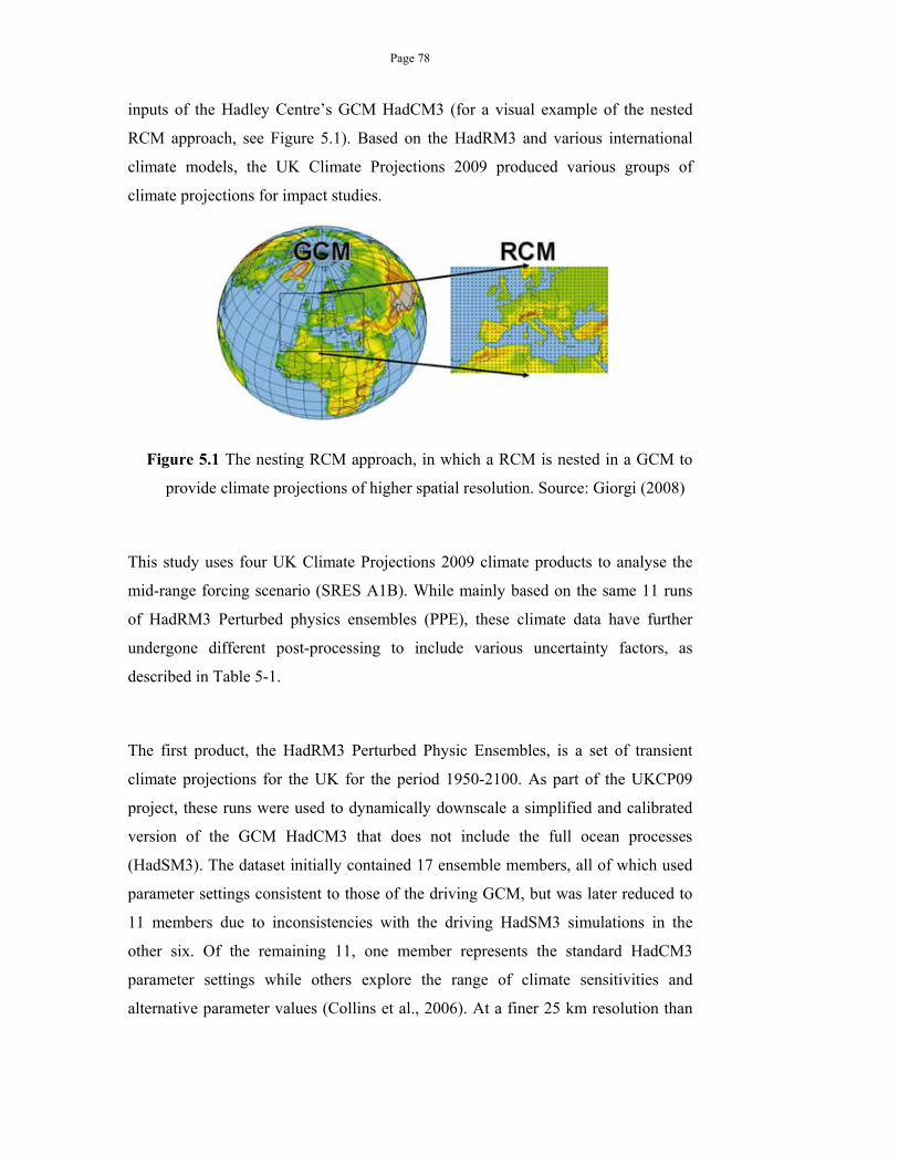
Page 78
inputs of the Hadley Centre’s GCM HadCM3 (for a visual example of the nested
RCM approach, see Figure 5.1). Based on the HadRM3 and various international
climate models, the UK Climate Projections 2009 produced various groups of
climate projections for impact studies.
Figure 5.1 The nesting RCM approach, in which a RCM is nested in a GCM to
provide climate projections of higher spatial resolution. Source: Giorgi (2008)
This study uses four UK Climate Projections 2009 climate products to analyse the
mid-range forcing scenario (SRES A1B). While mainly based on the same 11 runs
of HadRM3 Perturbed physics ensembles (PPE), these climate data have further
undergone different post-processing to include various uncertainty factors, as
described in Table 5-1.
The first product, the HadRM3 Perturbed Physic Ensembles, is a set of transient
climate projections for the UK for the period 1950-2100. As part of the UKCP09
project, these runs were used to dynamically downscale a simplified and calibrated
version of the GCM HadCM3 that does not include the full ocean processes
(HadSM3). The dataset initially contained 17 ensemble members, all of which used
parameter settings consistent to those of the driving GCM, but was later reduced to
11 members due to inconsistencies with the driving HadSM3 simulations in the
other six. Of the remaining 11, one member represents the standard HadCM3
parameter settings while others explore the range of climate sensitivities and
alternative parameter values (Collins et al., 2006). At a finer 25 km resolution than
Page 79
the GCM, the RCM runs use the GCM atmospheric dynamical and physical
processes; their boundary conditions come from the corresponding runs amongst 17
HadSM3 members, such as using the HadSM3 simulated time series of temperature
and wind. Therefore, they can further include regional physical processes but still
largely inherit the uncertainty from their driving GCM. They explore uncertainties in
the effects of varying regional physical processes, such as the effects of mountains,
coastlines and varying land surface properties.
The second product, the Spatially Coherent Projections (SCP), is close to the 11
RCM runs but has undergone additional post-processing to include a wider set of
uncertainties. As the HadRM3-PPE data only contains 11 members, they do not
sufficiently sample the uncertainty space that was probabilistically explored in the
fourth product: the UKCP09 Change Factors. In essence, the original RCMs did not
fully explore the uncertainty in global temperature from emission scenarios, carbon
cycle, sulphur cycle and ocean physics. In order to represent the spread that the
UKCP09 Change Factors consider, these RCM members were linearly scaled by
coefficients. These coefficients are representative of the global temperature changes
in the 10,000 Simple Climate Models that produced the UKCP09 dataset. The
results were analyzed for coefficient sets that best match UKCP09 data in terms of
winter and summer changes in temperature and precipitation for all 25 km grid
boxes over the UK for the period 2070–2099. Therefore, the SCPs can be considered
modified RCM runs that expand the uncertainty ranges to resemble those of
UKCP09, but bear the same limitations of RCMs, such as not including the
possibility of a mild increase in summer rainfall in Southern England (Sexton et al.,
2010).
The third product, the downscaled RCMs from the Future Flows project has an
increased spatial resolution compared to the other products. In particular, it is a
downscaled version of the 25-km- gridded RCMs into corresponding time series of 1
km grid boxes. Temporally, the original RCM data were statistically modified to
match the observations of the same decades within the 1950-2000 period. Spatially,
they are downscaled to reproduce the heterogeneity pattern of precipitation at the 1
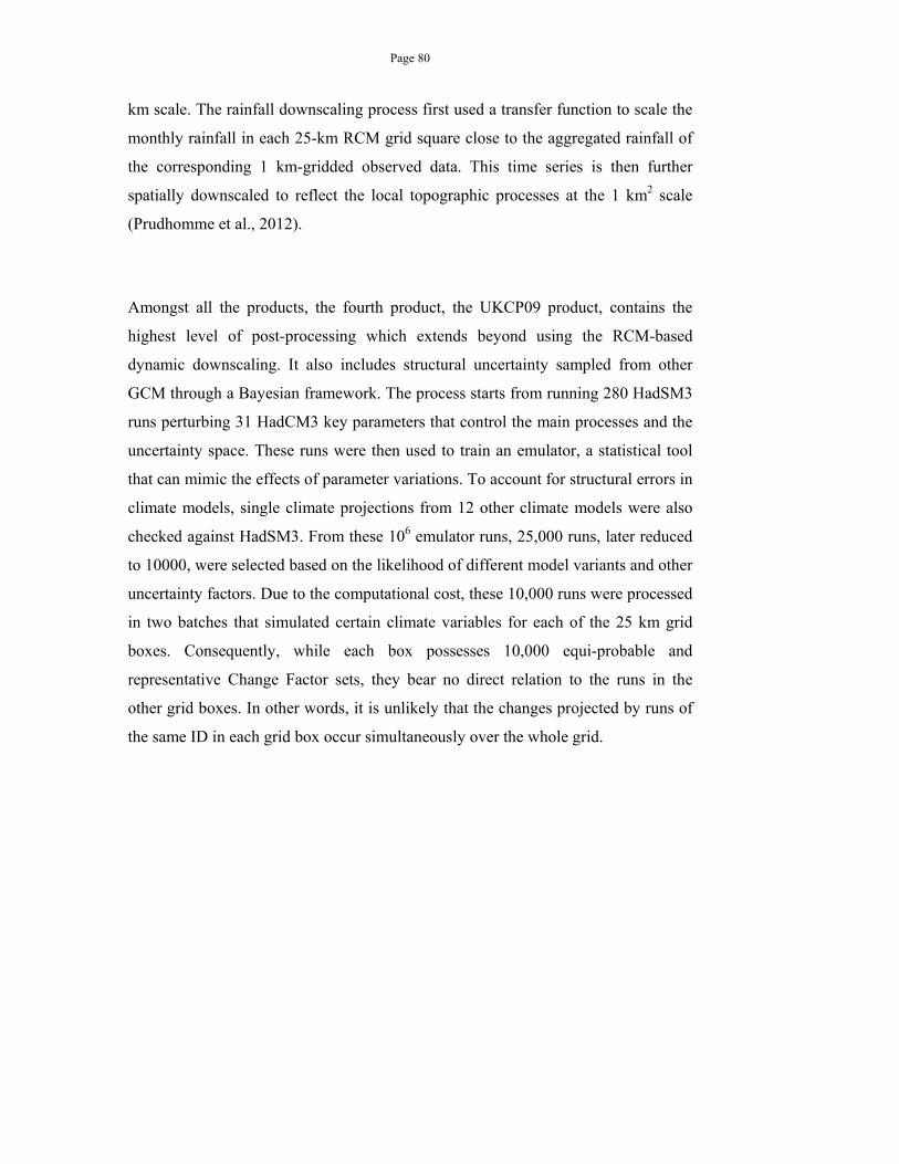
Page 80
km scale. The rainfall downscaling process first used a transfer function to scale the
monthly rainfall in each 25-km RCM grid square close to the aggregated rainfall of
the corresponding 1 km-gridded observed data. This time series is then further
spatially downscaled to reflect the local topographic processes at the 1 km2 scale
(Prudhomme et al., 2012).
Amongst all the products, the fourth product, the UKCP09 product, contains the
highest level of post-processing which extends beyond using the RCM-based
dynamic downscaling. It also includes structural uncertainty sampled from other
GCM through a Bayesian framework. The process starts from running 280 HadSM3
runs perturbing 31 HadCM3 key parameters that control the main processes and the
uncertainty space. These runs were then used to train an emulator, a statistical tool
that can mimic the effects of parameter variations. To account for structural errors in
climate models, single climate projections from 12 other climate models were also
checked against HadSM3. From these 106 emulator runs, 25,000 runs, later reduced
to 10000, were selected based on the likelihood of different model variants and other
uncertainty factors. Due to the computational cost, these 10,000 runs were processed
in two batches that simulated certain climate variables for each of the 25 km grid
boxes. Consequently, while each box possesses 10,000 equi-probable and
representative Change Factor sets, they bear no direct relation to the runs in the
other grid boxes. In other words, it is unlikely that the changes projected by runs of
the same ID in each grid box occur simultaneously over the whole grid.
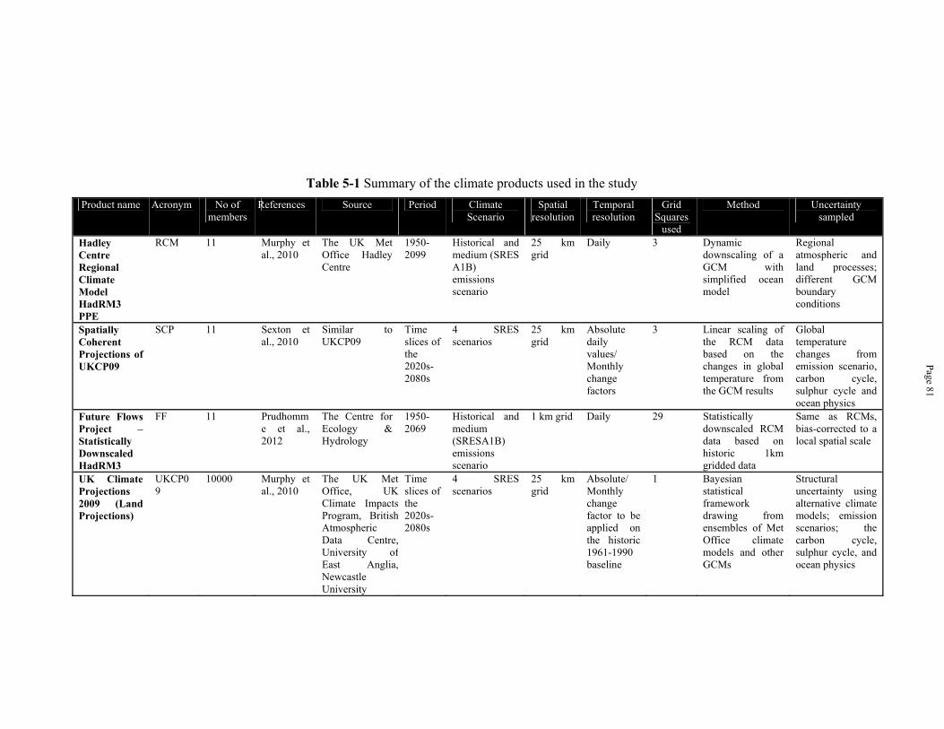
Page 81
Table 5-1 Summary of the climate products used in the study
Product name Acronym No of members
References Source Period Climate Scenario
Spatial resolution
Temporal resolution
Grid Squares
used
Method Uncertainty sampled
Hadley Centre Regional Climate Model HadRM3 PPE
RCM 11 Murphy et al., 2010
The UK Met Office Hadley Centre
1950-2099
Historical and medium (SRES A1B) emissions scenario
25 km grid
Daily 3 Dynamic downscaling of a GCM with simplified ocean model
Regional atmospheric and land processes; different GCM boundary conditions
Spatially Coherent Projections of UKCP09
SCP 11 Sexton et al., 2010
Similar to UKCP09
Time slices of the 2020s-2080s
4 SRES scenarios
25 km grid
Absolute daily values/ Monthly change factors
3 Linear scaling of the RCM data based on the changes in global temperature from the GCM results
Global temperature changes from emission scenario, carbon cycle, sulphur cycle and ocean physics
Future Flows Project – Statistically Downscaled HadRM3
FF 11 Prudhomme et al., 2012
The Centre for Ecology & Hydrology
1950-2069
Historical and medium (SRESA1B) emissions scenario
1 km grid Daily 29 Statistically downscaled RCM data based on historic 1km gridded data
Same as RCMs, bias-corrected to a local spatial scale
UK Climate Projections 2009 (Land Projections)
UKCP09
10000 Murphy et al., 2010
The UK Met Office, UK Climate Impacts Program, British Atmospheric Data Centre, University of East Anglia, Newcastle University
Time slices of the 2020s-2080s
4 SRES scenarios
25 km grid
Absolute/ Monthly change factor to be applied on the historic 1961-1990 baseline
1 Bayesian statistical framework drawing from ensembles of Met Office climate models and other GCMs
Structural uncertainty using alternative climate models; emission scenarios; the carbon cycle, sulphur cycle, and ocean physics
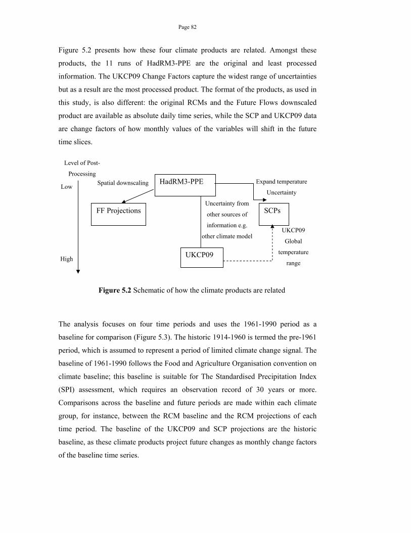
Page 82
Figure 5.2 presents how these four climate products are related. Amongst these
products, the 11 runs of HadRM3-PPE are the original and least processed
information. The UKCP09 Change Factors capture the widest range of uncertainties
but as a result are the most processed product. The format of the products, as used in
this study, is also different: the original RCMs and the Future Flows downscaled
product are available as absolute daily time series, while the SCP and UKCP09 data
are change factors of how monthly values of the variables will shift in the future
time slices.
Figure 5.2 Schematic of how the climate products are related
The analysis focuses on four time periods and uses the 1961-1990 period as a
baseline for comparison (Figure 5.3). The historic 1914-1960 is termed the pre-1961
period, which is assumed to represent a period of limited climate change signal. The
baseline of 1961-1990 follows the Food and Agriculture Organisation convention on
climate baseline; this baseline is suitable for The Standardised Precipitation Index
(SPI) assessment, which requires an observation record of 30 years or more.
Comparisons across the baseline and future periods are made within each climate
group, for instance, between the RCM baseline and the RCM projections of each
time period. The baseline of the UKCP09 and SCP projections are the historic
baseline, as these climate products project future changes as monthly change factors
of the baseline time series.
HadRM3-PPE
FF Projections
Spatial downscaling Expand temperature
Uncertainty
SCPs Uncertainty from
other sources of
information e.g.
other climate model
UKCP09
UKCP09
Global
temperature
range
Level of Post-
Processing
Low
High
Page 83
Figure 5.3 Time periods of interest in the study
5.2.2. Drought Indices
5.2.2.1.A brief review of drought indices
While most major drought indices recognise droughts as a prolonged period of
abnormal dryness, they use different indicators such as rainfall, river flows and soil
moisture deficits (Alley, 1984; Byun and Wilhite, 1999; Keyantash and Dracup,
2002; Morid et al., 2006; Smakhtin and Hughes, 2007). Major drought indices
include the Percent of Normal, Palmer Drought Severity Index (Palmer, 1965),
Standardised Precipitation Index (McKee et al., 1993; McKee et al., 1995), deciles
(Gibbons et al., 2008; Mpelasoka et al., 2008), Standardised Anomaly Index (Katz
and Glantz, 1986), the Effective Drought Index (Byun and Wilhite, 1999) and crop
moisture index (Palmer, 1968), as summarised by Table 5-2.
These indices indicate droughts as a cumulative deviation from the baseline period;
the deviation can be presented as an absolute value, a ratio of the standard deviation
or its rank in the total distribution. For instance, Effective Drought Index (EDI) is
the needed precipitation to counteract the accumulated deficit since drought onset
(Byun and Wilhite, 1996) while Palmer Drought Severity Index (PDSI) is a soil
moisture/water balance model that cumulatively measures surface water balance,
thus capable of indicating meteorological and hydrological droughts (Palmer, 1965;
Alley, 1985; Quiring and Papakryiakou, 2003). Palmer Drought Severity Index
1914-1960
2040-2069
2010-2039
1961-1990
2020-2049
Pre-1961
Baseline
The 2020s
The 2030s
The 2050s
Page 84
(PDSI), Standardised Precipitation Index (SPI), and Standardised Anomaly Index
(SAI) all standardise the baseline, thus facilitate comparison drought incidences
amongst different locations and periods. Various comparative studies show that
preferences and performance of drought indices vary: PDSI is popular in the US,
where it was derived; the decile index performs well for highly variable climate like
Australia and South Africa (Mpelasoka et al., 2008); while SPI may be comparable
to PDSI and river flows over various sites in the world (Guttman, 1998).
For the UK, Drought Severity Index (DSI) has been frequently used for studies
concerning drought spatial pattern (Phillips and McGregor, 1998; Fowler et al.,
2003; Rahiz and New, 2013) as well as a drought trigger for drought contingency
measures (Prudhomme et al., 2003; Southern Water, 2013). Meanwhile, SPI has
been used to assess pan-European drought incidences (Lloyd-Hughes and Saunders,
2002), Spain (Vicente-Serrano et al., 2010) and the UK (Vidal and Wade, 2009).
The analyses on UK droughts have revealed that drought occurrences, particularly in
the south-east, cluster spatially and temporally. As such, they pose great challenges
to water resource management that has to consider the risk of regional water supply
deficit spanning a prolonged period. Studies on future drought projections based on
both SPI and DSI (Blenkinsop and Fowler, 2007; Vidal and Wade, 2009) generally
indicate GCM as a major source of uncertainty, and that drought risk will gradually
increase particularly with regards to short and intense droughts of three to six
months.
As the next chapter will analyse hydrological droughts via a hydrological model,
this study focuses on meteorological drought analysis. The Standardised
Precipitation Index and the Standardised Precipitation-Evapotranspiration Index are
chosen as drought indices due to their robust capacity to identify droughts, their
simple data requirement and their ability to indicate droughts at various timescales.
The analysis will also link to hydrological and water management droughts assessed
in Chapter 6 to Chapter 9.
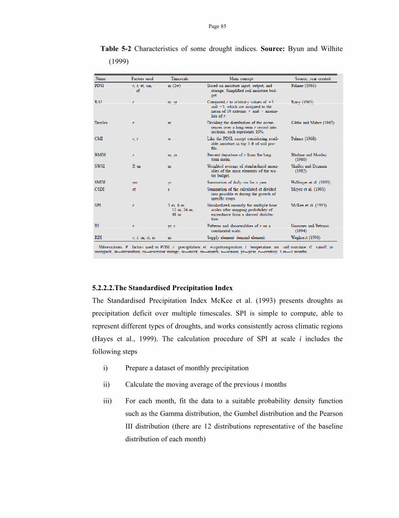
Page 85
Table 5-2 Characteristics of some drought indices. Source: Byun and Wilhite
(1999)
5.2.2.2.The Standardised Precipitation Index
The Standardised Precipitation Index McKee et al. (1993) presents droughts as
precipitation deficit over multiple timescales. SPI is simple to compute, able to
represent different types of droughts, and works consistently across climatic regions
(Hayes et al., 1999). The calculation procedure of SPI at scale i includes the
following steps
i) Prepare a dataset of monthly precipitation
ii) Calculate the moving average of the previous i months
iii) For each month, fit the data to a suitable probability density function
such as the Gamma distribution, the Gumbel distribution and the Pearson
III distribution (there are 12 distributions representative of the baseline
distribution of each month)
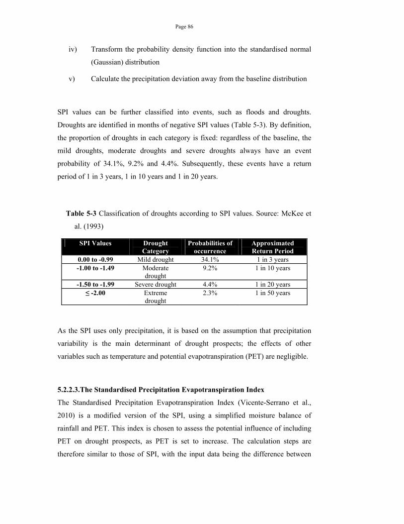
Page 86
iv) Transform the probability density function into the standardised normal
(Gaussian) distribution
v) Calculate the precipitation deviation away from the baseline distribution
SPI values can be further classified into events, such as floods and droughts.
Droughts are identified in months of negative SPI values (Table 5-3). By definition,
the proportion of droughts in each category is fixed: regardless of the baseline, the
mild droughts, moderate droughts and severe droughts always have an event
probability of 34.1%, 9.2% and 4.4%. Subsequently, these events have a return
period of 1 in 3 years, 1 in 10 years and 1 in 20 years.
Table 5-3 Classification of droughts according to SPI values. Source: McKee et
al. (1993)
SPI Values Drought Category
Probabilities of occurrence
Approximated Return Period
0.00 to -0.99 Mild drought 34.1% 1 in 3 years -1.00 to -1.49 Moderate
drought 9.2% 1 in 10 years
-1.50 to -1.99 Severe drought 4.4% 1 in 20 years ≤ -2.00 Extreme
drought 2.3% 1 in 50 years
As the SPI uses only precipitation, it is based on the assumption that precipitation
variability is the main determinant of drought prospects; the effects of other
variables such as temperature and potential evapotranspiration (PET) are negligible.
5.2.2.3.The Standardised Precipitation Evapotranspiration Index
The Standardised Precipitation Evapotranspiration Index (Vicente-Serrano et al.,
2010) is a modified version of the SPI, using a simplified moisture balance of
rainfall and PET. This index is chosen to assess the potential influence of including
PET on drought prospects, as PET is set to increase. The calculation steps are
therefore similar to those of SPI, with the input data being the difference between

Page 87
rainfall and PET. Drought categories are also kept the same as in Table 5-2. Similar
to SPI, the calculation procedure of SPEI at scale i includes the following steps:
i) Prepare a dataset of monthly precipitation subtracted by monthly PET
ii) Calculate the moving average of the previous i months
iii) For each month, fit the data to a suitable probability density function
such as the Gamma distribution, the log-normal distribution, the Gumbel
distribution and the Pearson III distribution (there are 12 distributions
representative of the baseline distribution of each month)
iv) Transform the probability density function into the standardised normal
(Gaussian) distribution
v) Calculate the precipitation deviation away from the baseline distribution
To identify a suitable probability distribution for SPEI fitting, Vicente-Serrano et al.
(2010) have used the L-moment ratio diagrams by Hosking (1990). “L” denotes
Linear and the L-moment is linear combinations of order statistics. It is computed as
the ratio of L skewness τ3 and L kurtosis τ4, which measures how skew to the left or
right and how peaky the shape of the distribution is. As the ratio of these measures
characterise different probabilistic distributions, they can be used to analyse whether
the empirical data are close any of these distributions in terms of the L-moment ratio
(Hosking, 1990). The diagram as such shows each group of distributions in
conjunction to the L-moment ratio of the empirical data.
Figure 5.4 demonstrates the L-moment ratio diagrams of the RCM, FF and Observed
monthly water balance data (which is monthly rainfall subtracted by monthly PET)
in comparison to the Generalised Logistic distributions (GLO), the Generalised
Extreme Value distributions (GEV), the Generalised Pareto distribution (GPA), the
Generalised Normal distribution (GNO) and the PearsonIII distribution (PE3). In
essence, the L-moment ratios were calculated for each month of the baseline 1961-
1990 time series of the observed data, the FF and the RCM product. Each month of a
time series is represented by an L-moment ratio, therefore becomes a point in the
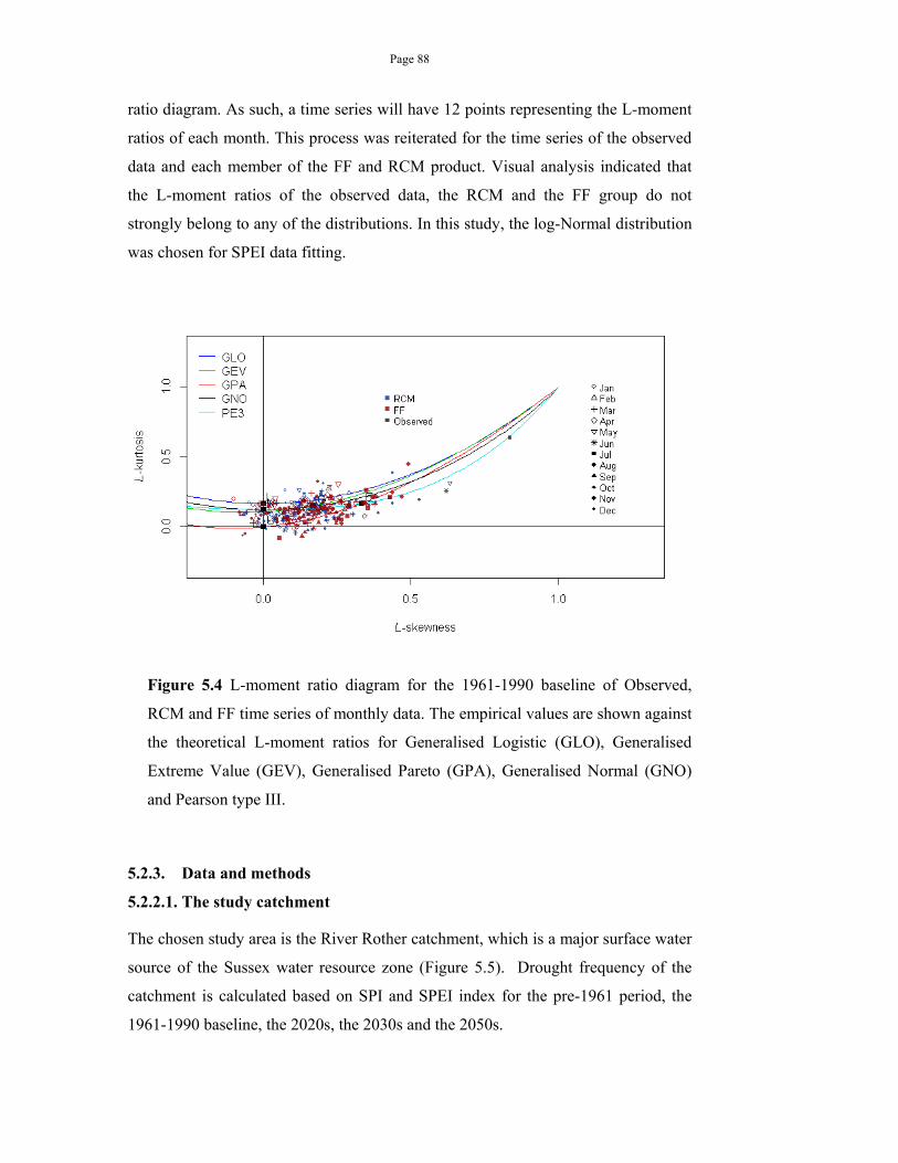
Page 88
ratio diagram. As such, a time series will have 12 points representing the L-moment
ratios of each month. This process was reiterated for the time series of the observed
data and each member of the FF and RCM product. Visual analysis indicated that
the L-moment ratios of the observed data, the RCM and the FF group do not
strongly belong to any of the distributions. In this study, the log-Normal distribution
was chosen for SPEI data fitting.
Figure 5.4 L-moment ratio diagram for the 1961-1990 baseline of Observed,
RCM and FF time series of monthly data. The empirical values are shown against
the theoretical L-moment ratios for Generalised Logistic (GLO), Generalised
Extreme Value (GEV), Generalised Pareto (GPA), Generalised Normal (GNO)
and Pearson type III.
5.2.3. Data and methods
5.2.2.1. The study catchment
The chosen study area is the River Rother catchment, which is a major surface water
source of the Sussex water resource zone (Figure 5.5). Drought frequency of the
catchment is calculated based on SPI and SPEI index for the pre-1961 period, the
1961-1990 baseline, the 2020s, the 2030s and the 2050s.
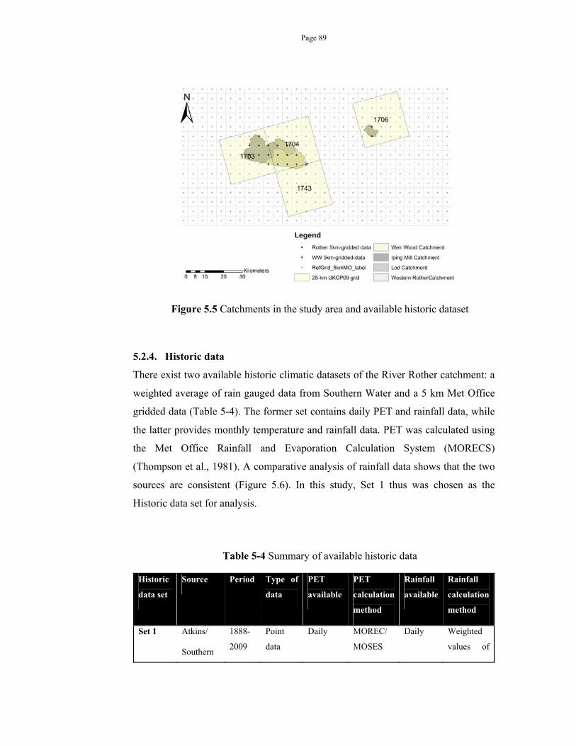
Page 89
Figure 5.5 Catchments in the study area and available historic dataset
5.2.4. Historic data
There exist two available historic climatic datasets of the River Rother catchment: a
weighted average of rain gauged data from Southern Water and a 5 km Met Office
gridded data (Table 5-4). The former set contains daily PET and rainfall data, while
the latter provides monthly temperature and rainfall data. PET was calculated using
the Met Office Rainfall and Evaporation Calculation System (MORECS)
(Thompson et al., 1981). A comparative analysis of rainfall data shows that the two
sources are consistent (Figure 5.6). In this study, Set 1 thus was chosen as the
Historic data set for analysis.
Table 5-4 Summary of available historic data
Historic
data set
Source Period Type of
data
PET
available
PET
calculation
method
Rainfall
available
Rainfall
calculation
method
Set 1 Atkins/
Southern
1888-
2009
Point
data
Daily MOREC/
MOSES
Daily Weighted
values of
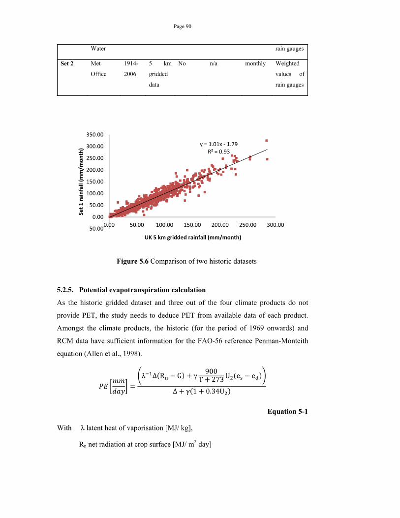
Page 90
Water rain gauges
Set 2 Met
Office
1914-
2006
5 km
gridded
data
No n/a monthly Weighted
values of
rain gauges
Figure 5.6 Comparison of two historic datasets
5.2.5. Potential evapotranspiration calculation
As the historic gridded dataset and three out of the four climate products do not
provide PET, the study needs to deduce PET from available data of each product.
Amongst the climate products, the historic (for the period of 1969 onwards) and
RCM data have sufficient information for the FAO-56 reference Penman-Monteith
equation (Allen et al., 1998).
λ Δ R G γ 900T 273U e e
Δ γ 1 0.34U
Equation 5-1
With λ latent heat of vaporisation [MJ/ kg],
Rn net radiation at crop surface [MJ/ m2 day]
y = 1.01x ‐ 1.79R² = 0.93
‐50.00
0.00
50.00
100.00
150.00
200.00
250.00
300.00
350.00
0.00 50.00 100.00 150.00 200.00 250.00 300.00
Set 1 rainfall (m
m/m
onth)
UK 5 km gridded rainfall (mm/month)
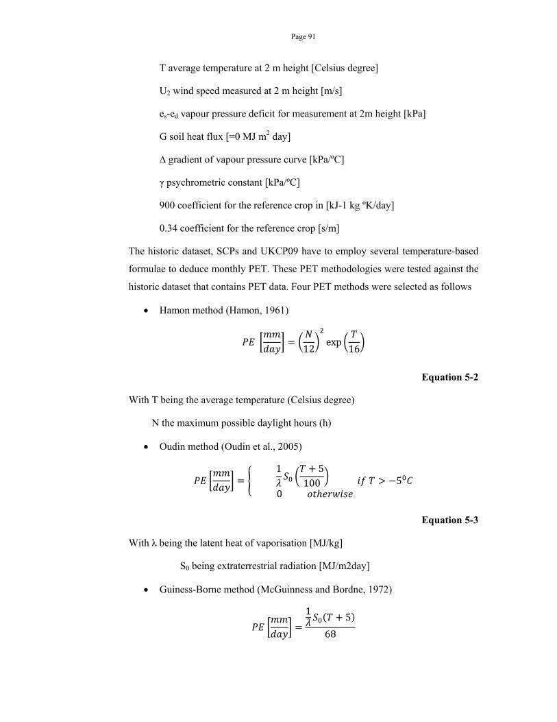
Page 91
T average temperature at 2 m height [Celsius degree]
U2 wind speed measured at 2 m height [m/s]
es-ed vapour pressure deficit for measurement at 2m height [kPa]
G soil heat flux [=0 MJ m2 day]
∆ gradient of vapour pressure curve [kPa/ºC]
γ psychrometric constant [kPa/ºC]
900 coefficient for the reference crop in [kJ-1 kg ºK/day]
0.34 coefficient for the reference crop [s/m]
The historic dataset, SCPs and UKCP09 have to employ several temperature-based
formulae to deduce monthly PET. These PET methodologies were tested against the
historic dataset that contains PET data. Four PET methods were selected as follows
Hamon method (Hamon, 1961)
12
exp16
Equation 5-2
With T being the average temperature (Celsius degree)
N the maximum possible daylight hours (h)
Oudin method (Oudin et al., 2005)
1 5100
0 5
Equation 5-3
With λ being the latent heat of vaporisation [MJ/kg]
S0 being extraterrestrial radiation [MJ/m2day]
Guiness-Borne method (McGuinness and Bordne, 1972)
15
68
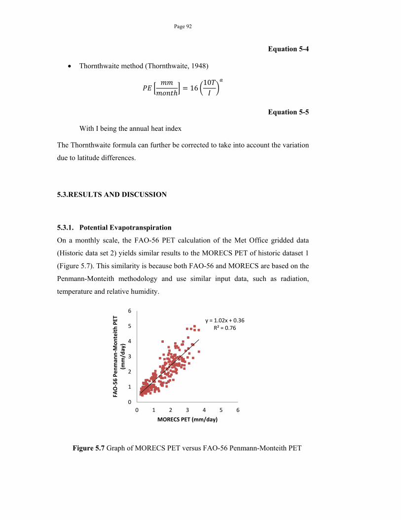
Page 92
Equation 5-4
Thornthwaite method (Thornthwaite, 1948)
1610
Equation 5-5
With I being the annual heat index
The Thornthwaite formula can further be corrected to take into account the variation
due to latitude differences.
5.3.RESULTS AND DISCUSSION
5.3.1. Potential Evapotranspiration
On a monthly scale, the FAO-56 PET calculation of the Met Office gridded data
(Historic data set 2) yields similar results to the MORECS PET of historic dataset 1
(Figure 5.7). This similarity is because both FAO-56 and MORECS are based on the
Penmann-Monteith methodology and use similar input data, such as radiation,
temperature and relative humidity.
Figure 5.7 Graph of MORECS PET versus FAO-56 Penmann-Monteith PET
y = 1.02x + 0.36R² = 0.76
0
1
2
3
4
5
6
0 1 2 3 4 5 6
FAO‐56 Penman
n‐M
onteith PET
(m
m/day)
MORECS PET (mm/day)
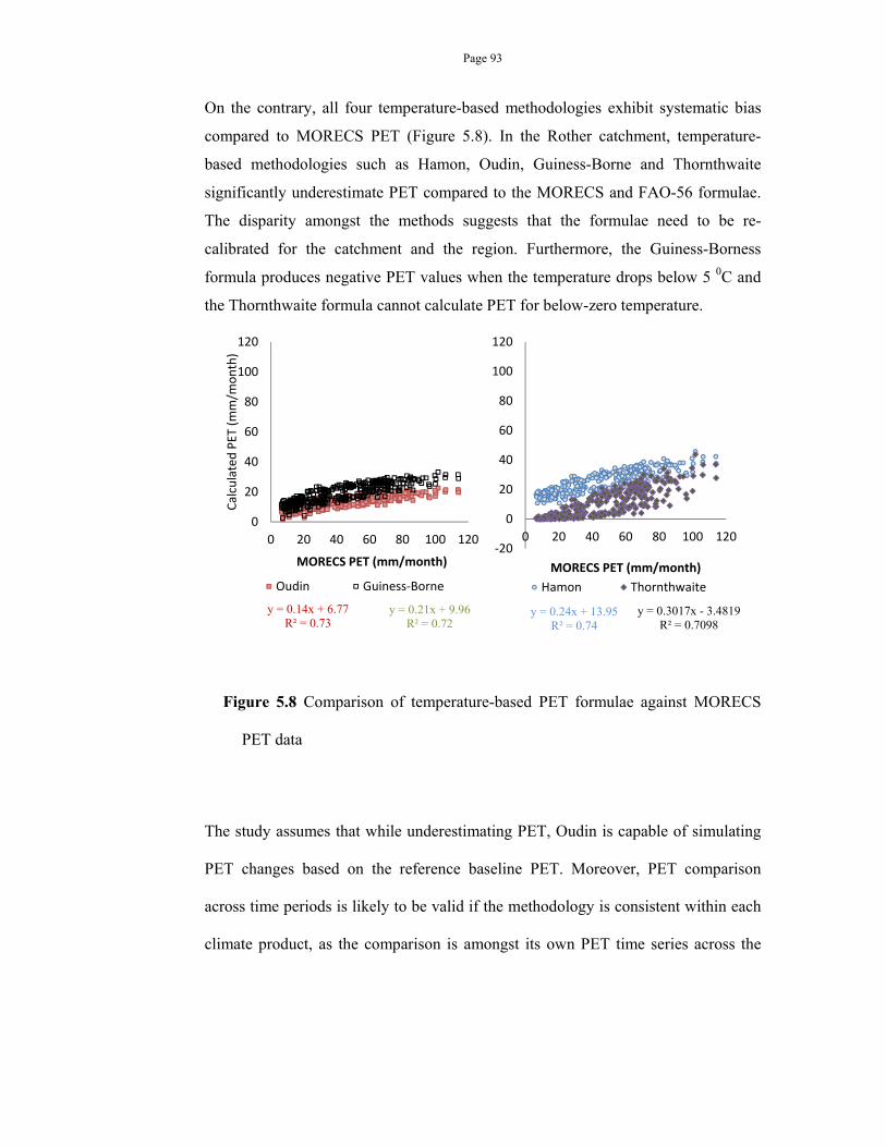
Page 93
On the contrary, all four temperature-based methodologies exhibit systematic bias
compared to MORECS PET (Figure 5.8). In the Rother catchment, temperature-
based methodologies such as Hamon, Oudin, Guiness-Borne and Thornthwaite
significantly underestimate PET compared to the MORECS and FAO-56 formulae.
The disparity amongst the methods suggests that the formulae need to be re-
calibrated for the catchment and the region. Furthermore, the Guiness-Borness
formula produces negative PET values when the temperature drops below 5 0C and
the Thornthwaite formula cannot calculate PET for below-zero temperature.
Figure 5.8 Comparison of temperature-based PET formulae against MORECS
PET data
The study assumes that while underestimating PET, Oudin is capable of simulating
PET changes based on the reference baseline PET. Moreover, PET comparison
across time periods is likely to be valid if the methodology is consistent within each
climate product, as the comparison is amongst its own PET time series across the
y = 0.14x + 6.77R² = 0.73
y = 0.21x + 9.96R² = 0.72
0
20
40
60
80
100
120
0 20 40 60 80 100 120
Calculated PET (mm/m
onth)
MORECS PET (mm/month)
Oudin Guiness‐Borne
y = 0.24x + 13.95R² = 0.74
y = 0.3017x - 3.4819R² = 0.7098
‐20
0
20
40
60
80
100
120
0 20 40 60 80 100 120
MORECS PET (mm/month)
Hamon Thornthwaite
Page 94
time periods. For each climate product, the PET methodologies are thus selected as
follows
RCM data: The FAO-56 Penmann Monteith method was selected, since the
projections provide sufficient input data for the method.
FF data: PET is readily provided in the product. This product uses the FAO-
56 Penmann Monteith to calculate PET.
Historic observed data, UKCP09 and SCP: Amongst the PET
methodologies, the Oudin method was selected, since it can work over a
wide range of temperature and has a simple mathematical form for potential
recalibration. In this study, such calibration was not conducted due to the
time constraints. However, potential PET underestimation was
acknowledged and taken into consideration in the analysis. While it is
preferable to use the Oudin method across all of the three dataset, the
analysis on historic data shows that the Oudin equation significantly
underestimates PET. Thus the MORECS historic PET was chosen as the
historic baseline PET, in order to reflect the true historic balance between
rainfall and PET. PET changes due to increased temperature was then
simulated using the Oudin equation. In essence, the Oudin equation assumes
that PET changes with T as follows
1 5100
0 5
Equation 5-6
With λ being the latent heat of vaporization [MJ/kg]
Page 95
S0 being extraterrestrial radiation [MJ/m2day]
Assuming that S0 and λ remain constant and all PE for temperature below -5 0C are
0, an increased PE due to increase temperature can be written as
1 5100
0
5
Equation 5-7
If we divide the first equation by the second equation, it follows that
5
5 5
As Tchange=T(1+CF)
1 5
0 5 5 >-5
Equation 5-8
The formula does not work in the case of T< -5, as PE=0, it follows that PEchange=0
regardless of Tchange. However, the monthly temperature time series of the Rother
catchment does not contain any value below this threshold; the consideration of this
case was thus avoided.
5.3.2. Analysis of the climate products
5.3.2.1.Comparison with observations
Two of the climate products (RCM and FF) were compared with past observations
(Figure 5.9). Within the historic period of 1961-1990, the RCM runs already exhibit
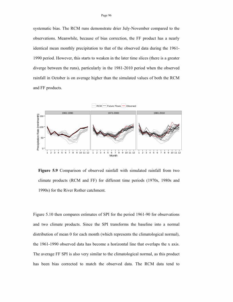
Page 96
systematic bias. The RCM runs demonstrate drier July-November compared to the
observations. Meanwhile, because of bias correction, the FF product has a nearly
identical mean monthly precipitation to that of the observed data during the 1961-
1990 period. However, this starts to weaken in the later time slices (there is a greater
diverge between the runs), particularly in the 1981-2010 period when the observed
rainfall in October is on average higher than the simulated values of both the RCM
and FF products.
Figure 5.9 Comparison of observed rainfall with simulated rainfall from two
climate products (RCM and FF) for different time periods (1970s, 1980s and
1990s) for the River Rother catchment.
Figure 5.10 then compares estimates of SPI for the period 1961-90 for observations
and two climate products. Since the SPI transforms the baseline into a normal
distribution of mean 0 for each month (which represents the climatological normal),
the 1961-1990 observed data has become a horizontal line that overlaps the x axis.
The average FF SPI is also very similar to the climatological normal, as this product
has been bias corrected to match the observed data. The RCM data tend to
1961-1990 1971-2000 1981-2010
0
50
100
150
1 2 3 4 5 6 7 8 9 10 11 12 1 2 3 4 5 6 7 8 9 10 11 12 1 2 3 4 5 6 7 8 9 10 11 12Month
Pre
cipi
tatio
n R
ate
(m
m/m
onth
)
RCM Future Flows Observed
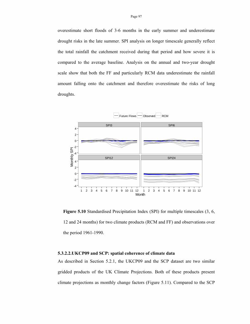
Page 97
overestimate short floods of 3-6 months in the early summer and underestimate
drought risks in the late summer. SPI analysis on longer timescale generally reflect
the total rainfall the catchment received during that period and how severe it is
compared to the average baseline. Analysis on the annual and two-year drought
scale show that both the FF and particularly RCM data underestimate the rainfall
amount falling onto the catchment and therefore overestimate the risks of long
droughts.
Figure 5.10 Standardised Precipitation Index (SPI) for multiple timescales (3, 6,
12 and 24 months) for two climate products (RCM and FF) and observations over
the period 1961-1990.
5.3.2.2.UKCP09 and SCP: spatial coherence of climate data
As described in Section 5.2.1, the UKCP09 and the SCP dataset are two similar
gridded products of the UK Climate Projections. Both of these products present
climate projections as monthly change factors (Figure 5.11). Compared to the SCP
SPI3 SPI6
SPI12 SPI24
-4
-2
0
2
4
-4
-2
0
2
4
1 2 3 4 5 6 7 8 9 10 11 12 1 2 3 4 5 6 7 8 9 10 11 12Month
Mo
nth
ly S
PI
Future Flows Observed RCM
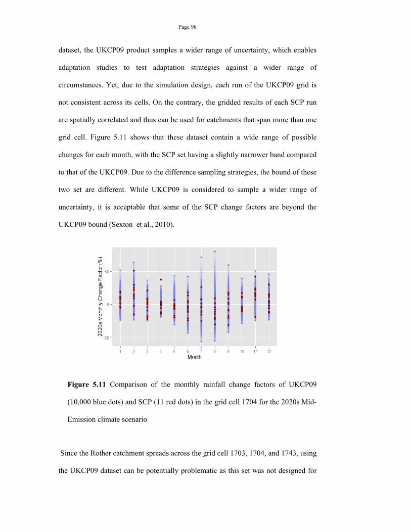
Page 98
dataset, the UKCP09 product samples a wider range of uncertainty, which enables
adaptation studies to test adaptation strategies against a wider range of
circumstances. Yet, due to the simulation design, each run of the UKCP09 grid is
not consistent across its cells. On the contrary, the gridded results of each SCP run
are spatially correlated and thus can be used for catchments that span more than one
grid cell. Figure 5.11 shows that these dataset contain a wide range of possible
changes for each month, with the SCP set having a slightly narrower band compared
to that of the UKCP09. Due to the difference sampling strategies, the bound of these
two set are different. While UKCP09 is considered to sample a wider range of
uncertainty, it is acceptable that some of the SCP change factors are beyond the
UKCP09 bound (Sexton et al., 2010).
Figure 5.11 Comparison of the monthly rainfall change factors of UKCP09
(10,000 blue dots) and SCP (11 red dots) in the grid cell 1704 for the 2020s Mid-
Emission climate scenario
Since the Rother catchment spreads across the grid cell 1703, 1704, and 1743, using
the UKCP09 dataset can be potentially problematic as this set was not designed for
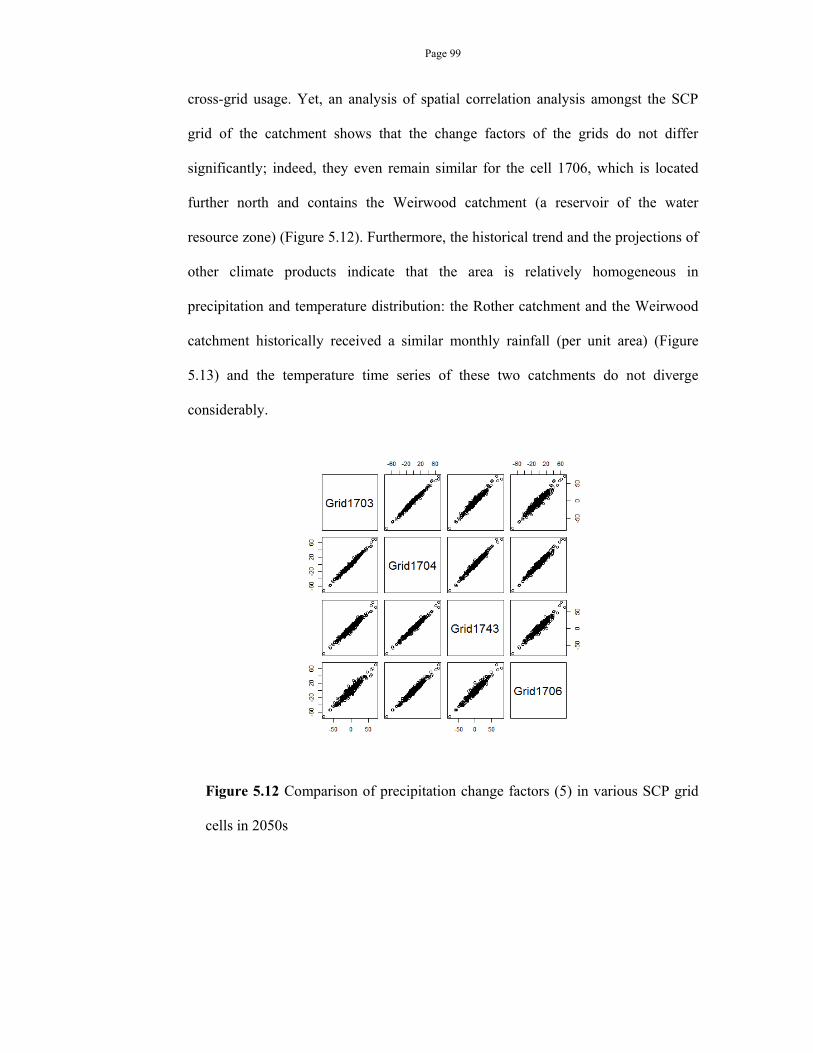
Page 99
cross-grid usage. Yet, an analysis of spatial correlation analysis amongst the SCP
grid of the catchment shows that the change factors of the grids do not differ
significantly; indeed, they even remain similar for the cell 1706, which is located
further north and contains the Weirwood catchment (a reservoir of the water
resource zone) (Figure 5.12). Furthermore, the historical trend and the projections of
other climate products indicate that the area is relatively homogeneous in
precipitation and temperature distribution: the Rother catchment and the Weirwood
catchment historically received a similar monthly rainfall (per unit area) (Figure
5.13) and the temperature time series of these two catchments do not diverge
considerably.
Figure 5.12 Comparison of precipitation change factors (5) in various SCP grid
cells in 2050s
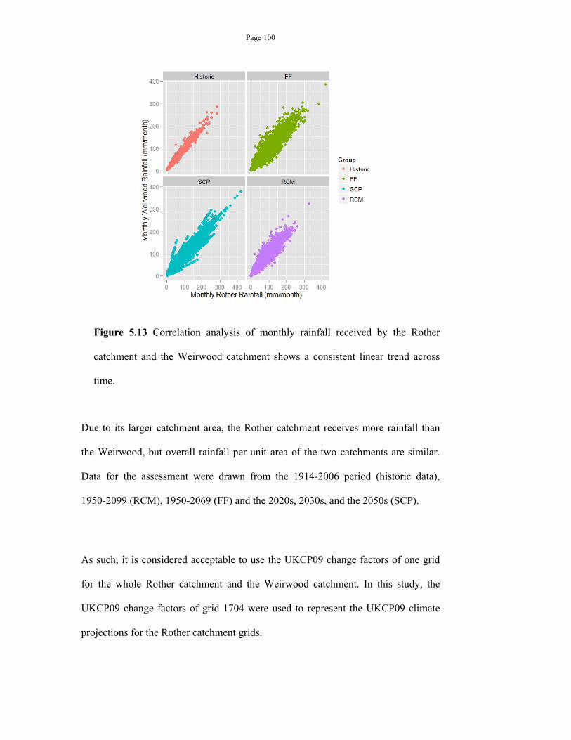
Page 100
Figure 5.13 Correlation analysis of monthly rainfall received by the Rother
catchment and the Weirwood catchment shows a consistent linear trend across
time.
Due to its larger catchment area, the Rother catchment receives more rainfall than
the Weirwood, but overall rainfall per unit area of the two catchments are similar.
Data for the assessment were drawn from the 1914-2006 period (historic data),
1950-2099 (RCM), 1950-2069 (FF) and the 2020s, 2030s, and the 2050s (SCP).
As such, it is considered acceptable to use the UKCP09 change factors of one grid
for the whole Rother catchment and the Weirwood catchment. In this study, the
UKCP09 change factors of grid 1704 were used to represent the UKCP09 climate
projections for the Rother catchment grids.
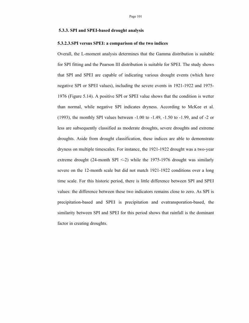
Page 101
5.3.3. SPI and SPEI-based drought analysis
5.3.2.3.SPI versus SPEI: a comparison of the two indices
Overall, the L-moment analysis determines that the Gamma distribution is suitable
for SPI fitting and the Pearson III distribution is suitable for SPEI. The study shows
that SPI and SPEI are capable of indicating various drought events (which have
negative SPI or SPEI values), including the severe events in 1921-1922 and 1975-
1976 (Figure 5.14). A positive SPI or SPEI value shows that the condition is wetter
than normal, while negative SPI indicates dryness. According to McKee et al.
(1993), the monthly SPI values between -1.00 to -1.49, -1.50 to -1.99, and of -2 or
less are subsequently classified as moderate droughts, severe droughts and extreme
droughts. Aside from drought classification, these indices are able to demonstrate
dryness on multiple timescales. For instance, the 1921-1922 drought was a two-year
extreme drought (24-month SPI <-2) while the 1975-1976 drought was similarly
severe on the 12-month scale but did not match 1921-1922 conditions over a long
time scale. For this historic period, there is little difference between SPI and SPEI
values: the difference between these two indicators remains close to zero. As SPI is
precipitation-based and SPEI is precipitation and evatransporation-based, the
similarity between SPI and SPEI for this period shows that rainfall is the dominant
factor in creating droughts.
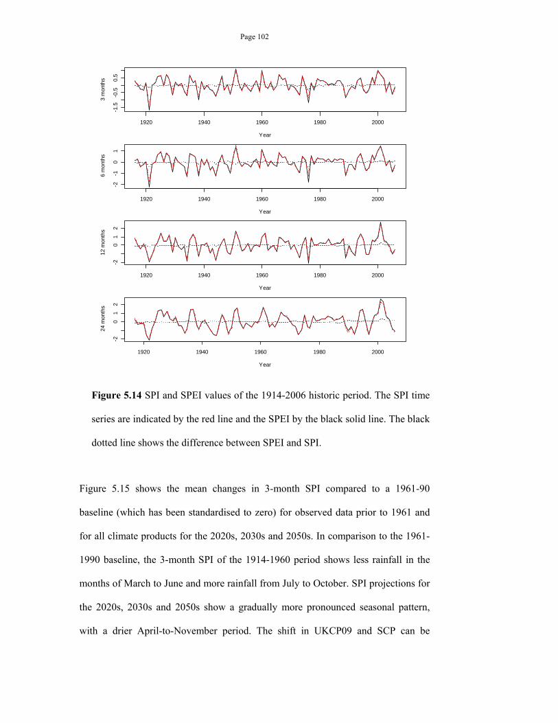
Page 102
Figure 5.14 SPI and SPEI values of the 1914-2006 historic period. The SPI time
series are indicated by the red line and the SPEI by the black solid line. The black
dotted line shows the difference between SPEI and SPI.
Figure 5.15 shows the mean changes in 3-month SPI compared to a 1961-90
baseline (which has been standardised to zero) for observed data prior to 1961 and
for all climate products for the 2020s, 2030s and 2050s. In comparison to the 1961-
1990 baseline, the 3-month SPI of the 1914-1960 period shows less rainfall in the
months of March to June and more rainfall from July to October. SPI projections for
the 2020s, 2030s and 2050s show a gradually more pronounced seasonal pattern,
with a drier April-to-November period. The shift in UKCP09 and SCP can be
1920 1940 1960 1980 2000-1
.5-0
.50.
5
Year
3 m
onth
s
1920 1940 1960 1980 2000
-2-1
01
Year
6 m
onth
s
1920 1940 1960 1980 2000
-20
12
Year
12
mon
ths
1920 1940 1960 1980 2000
-20
12
Year
24
mon
ths
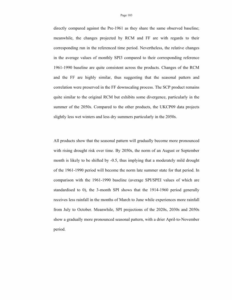
Page 103
directly compared against the Pre-1961 as they share the same observed baseline;
meanwhile, the changes projected by RCM and FF are with regards to their
corresponding run in the referenced time period. Nevertheless, the relative changes
in the average values of monthly SPI3 compared to their corresponding reference
1961-1990 baseline are quite consistent across the products. Changes of the RCM
and the FF are highly similar, thus suggesting that the seasonal pattern and
correlation were preserved in the FF downscaling process. The SCP product remains
quite similar to the original RCM but exhibits some divergence, particularly in the
summer of the 2050s. Compared to the other products, the UKCP09 data projects
slightly less wet winters and less dry summers particularly in the 2050s.
All products show that the seasonal pattern will gradually become more pronounced
with rising drought risk over time. By 2050s, the norm of an August or September
month is likely to be shifted by -0.5, thus implying that a moderately mild drought
of the 1961-1990 period will become the norm late summer state for that period. In
comparison with the 1961-1990 baseline (average SPI/SPEI values of which are
standardised to 0), the 3-month SPI shows that the 1914-1960 period generally
receives less rainfall in the months of March to June while experiences more rainfall
from July to October. Meanwhile, SPI projections of the 2020s, 2030s and 2050s
show a gradually more pronounced seasonal pattern, with a drier April-to-November
period.
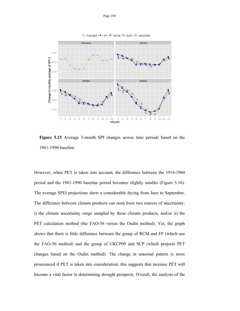
Page 104
Figure 5.15 Average 3-month SPI changes across time periods based on the
1961-1990 baseline
However, when PET is taken into account, the difference between the 1914-1960
period and the 1961-1990 baseline period becomes slightly smaller (Figure 5.16).
The average SPEI projections show a considerable drying from June to September.
The difference between climate products can stem from two sources of uncertainty:
i) the climate uncertainty range sampled by these climate products, and/or ii) the
PET calculation method (the FAO-56 versus the Oudin method). Yet, the graph
shows that there is little difference between the group of RCM and FF (which use
the FAO-56 method) and the group of UKCP09 and SCP (which projects PET
changes based on the Oudin method). The change in seasonal pattern is more
pronounced if PET is taken into consideration; this suggests that increase PET will
become a vital factor in determining drought prospects. Overall, the analysis of the
Historic 2020s
2030s 2050s
-0.5
0.0
0.5
-0.5
0.0
0.5
1 2 3 4 5 6 7 8 9 10 11 12 1 2 3 4 5 6 7 8 9 10 11 12Month
Change in
month
ly a
vera
ge o
f SP
I 3
Pre1961 FF RCM SCP UKCP09
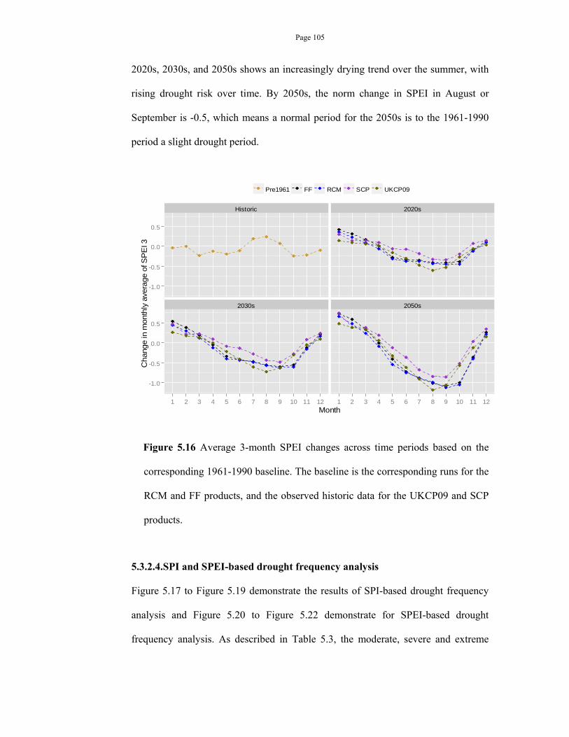
Page 105
2020s, 2030s, and 2050s shows an increasingly drying trend over the summer, with
rising drought risk over time. By 2050s, the norm change in SPEI in August or
September is -0.5, which means a normal period for the 2050s is to the 1961-1990
period a slight drought period.
Figure 5.16 Average 3-month SPEI changes across time periods based on the
corresponding 1961-1990 baseline. The baseline is the corresponding runs for the
RCM and FF products, and the observed historic data for the UKCP09 and SCP
products.
5.3.2.4.SPI and SPEI-based drought frequency analysis
Figure 5.17 to Figure 5.19 demonstrate the results of SPI-based drought frequency
analysis and Figure 5.20 to Figure 5.22 demonstrate for SPEI-based drought
frequency analysis. As described in Table 5.3, the moderate, severe and extreme
Historic 2020s
2030s 2050s
-1.0
-0.5
0.0
0.5
-1.0
-0.5
0.0
0.5
1 2 3 4 5 6 7 8 9 10 11 12 1 2 3 4 5 6 7 8 9 10 11 12Month
Change in
month
ly a
vera
ge o
f SP
EI 3
Pre1961 FF RCM SCP UKCP09
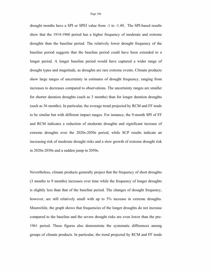
Page 106
drought months have a SPI or SPEI value from -1 to -1.49, The SPI-based results
show that the 1914-1960 period has a higher frequency of moderate and extreme
droughts than the baseline period. The relatively lower drought frequency of the
baseline period suggests that the baseline period could have been extended to a
longer period. A longer baseline period would have captured a wider range of
drought types and magnitude, as droughts are rare extreme events. Climate products
show large ranges of uncertainty in estimates of drought frequency, ranging from
increases to decreases compared to observations. The uncertainty ranges are smaller
for shorter duration droughts (such as 3 months) than for longer duration droughts
(such as 36 months). In particular, the average trend projected by RCM and FF tends
to be similar but with different impact ranges. For instance, the 9-month SPI of FF
and RCM indicates a reduction of moderate droughts and significant increase of
extreme droughts over the 2020s-2050s period, while SCP results indicate an
increasing risk of moderate drought risks and a slow growth of extreme drought risk
in 2020s-2030s and a sudden jump in 2050s.
Nevertheless, climate products generally project that the frequency of short droughts
(3 months to 9 months) increases over time while the frequency of longer droughts
is slightly less than that of the baseline period. The changes of drought frequency,
however, are still relatively small with up to 5% increase in extreme droughts.
Meanwhile, the graph shows that frequencies of the longer droughts do not increase
compared to the baseline and the severe drought risks are even lower than the pre-
1961 period. These figures also demonstrate the systematic differences among
groups of climate products. In particular, the trend projected by RCM and FF tends
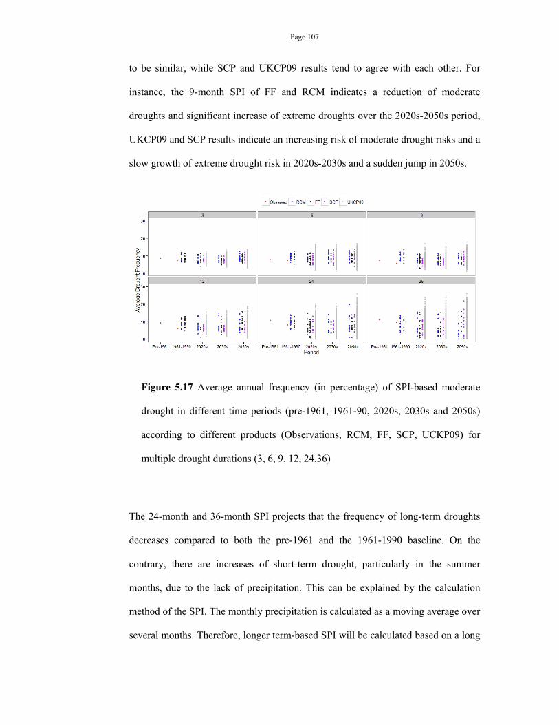
Page 107
to be similar, while SCP and UKCP09 results tend to agree with each other. For
instance, the 9-month SPI of FF and RCM indicates a reduction of moderate
droughts and significant increase of extreme droughts over the 2020s-2050s period,
UKCP09 and SCP results indicate an increasing risk of moderate drought risks and a
slow growth of extreme drought risk in 2020s-2030s and a sudden jump in 2050s.
Figure 5.17 Average annual frequency (in percentage) of SPI-based moderate
drought in different time periods (pre-1961, 1961-90, 2020s, 2030s and 2050s)
according to different products (Observations, RCM, FF, SCP, UCKP09) for
multiple drought durations (3, 6, 9, 12, 24,36)
The 24-month and 36-month SPI projects that the frequency of long-term droughts
decreases compared to both the pre-1961 and the 1961-1990 baseline. On the
contrary, there are increases of short-term drought, particularly in the summer
months, due to the lack of precipitation. This can be explained by the calculation
method of the SPI. The monthly precipitation is calculated as a moving average over
several months. Therefore, longer term-based SPI will be calculated based on a long
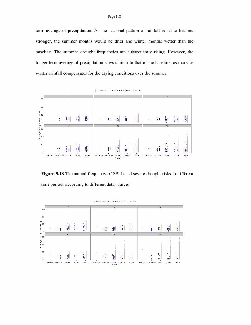
Page 108
term average of precipitation. As the seasonal pattern of rainfall is set to become
stronger, the summer months would be drier and winter months wetter than the
baseline. The summer drought frequencies are subsequently rising. However, the
longer term average of precipitation stays similar to that of the baseline, as increase
winter rainfall compensates for the drying conditions over the summer.
Figure 5.18 The annual frequency of SPI-based severe drought risks in different
time periods according to different data sources
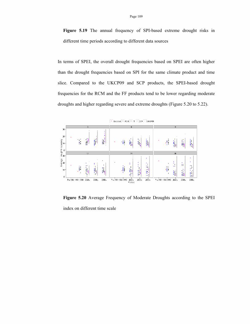
Page 109
Figure 5.19 The annual frequency of SPI-based extreme drought risks in
different time periods according to different data sources
In terms of SPEI, the overall drought frequencies based on SPEI are often higher
than the drought frequencies based on SPI for the same climate product and time
slice. Compared to the UKCP09 and SCP products, the SPEI-based drought
frequencies for the RCM and the FF products tend to be lower regarding moderate
droughts and higher regarding severe and extreme droughts (Figure 5.20 to 5.22).
Figure 5.20 Average Frequency of Moderate Droughts according to the SPEI
index on different time scale
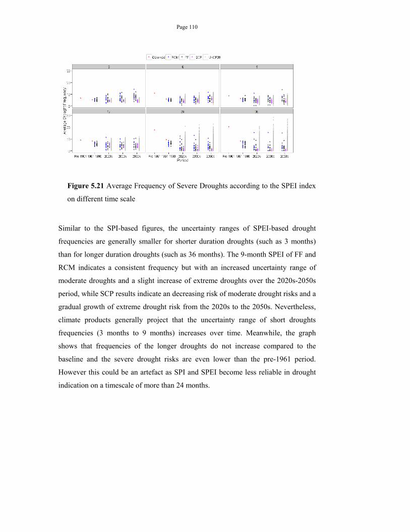
Page 110
Figure 5.21 Average Frequency of Severe Droughts according to the SPEI index
on different time scale
Similar to the SPI-based figures, the uncertainty ranges of SPEI-based drought
frequencies are generally smaller for shorter duration droughts (such as 3 months)
than for longer duration droughts (such as 36 months). The 9-month SPEI of FF and
RCM indicates a consistent frequency but with an increased uncertainty range of
moderate droughts and a slight increase of extreme droughts over the 2020s-2050s
period, while SCP results indicate an decreasing risk of moderate drought risks and a
gradual growth of extreme drought risk from the 2020s to the 2050s. Nevertheless,
climate products generally project that the uncertainty range of short droughts
frequencies (3 months to 9 months) increases over time. Meanwhile, the graph
shows that frequencies of the longer droughts do not increase compared to the
baseline and the severe drought risks are even lower than the pre-1961 period.
However this could be an artefact as SPI and SPEI become less reliable in drought
indication on a timescale of more than 24 months.
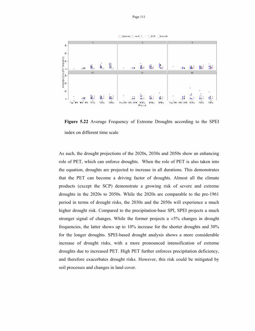
Page 111
Figure 5.22 Average Frequency of Extreme Droughts according to the SPEI
index on different time scale
As such, the drought projections of the 2020s, 2030s and 2050s show an enhancing
role of PET, which can enforce droughts. When the role of PET is also taken into
the equation, droughts are projected to increase in all durations. This demonstrates
that the PET can become a driving factor of droughts. Almost all the climate
products (except the SCP) demonstrate a growing risk of severe and extreme
droughts in the 2020s to 2050s. While the 2020s are comparable to the pre-1961
period in terms of drought risks, the 2030s and the 2050s will experience a much
higher drought risk. Compared to the precipitation-base SPI, SPEI projects a much
stronger signal of changes. While the former projects a ±5% changes in drought
frequencies, the latter shows up to 10% increase for the shorter droughts and 30%
for the longer droughts. SPEI-based drought analysis shows a more considerable
increase of drought risks, with a more pronounced intensification of extreme
droughts due to increased PET. High PET further enforces precipitation deficiency,
and therefore exacerbates drought risks. However, this risk could be mitigated by
soil processes and changes in land cover.
Page 112
The index of SPEI also demonstrates structural uncertainty amongst the climate
products, with RCM projecting a relatively higher drought risk compared to FF,
UKCP09 and SCP. On the contrary, FF, a bias-corrected product of RCM, shows a
slightly lower change in drought frequencies. The risk and uncertainty envelope of
extreme droughts appear to increase over time, with the 2020s period having similar
drought frequencies to those of the 1914-1960 period. However, natural climate
variability may still dominate the 2020s and 2030s, as Kendon et al. (2008) has
shown that climate change signals can only be inferred with more than three 30-year
projection periods. With SPEI, the systematic differences among the climate
products persist. These differences might stem from three factors:
The difference in sampled uncertainty of each climate product (as described
in Table 5.1)
The difference in the post-processing approach, such as bias correction,
downscaling and resampling
The difference PET calculation approaches, as the PETs of RCM and FF are
Penmann-Monteith-based while PET changes of UKCP09 and SCP are
Oudin-based
Natural variability
Amongst all the considered climate products, SCP seems to consistently project the
lowest change of drought risks while RCM produces the highest. It is noted that
while RCM was known to significantly overestimate the drying condition, such bias
was to an extent compensated by comparing changes within the same RCM runs. As
such, although the historic RCM baseline (1961-1990) is drier than the observation
data, the RCM future changes of drought risks is calculated based on the RCM
baseline.
Finally, while the structural difference of the climate products are likely to cause the
dissimilar drought projections, the results show that using different PET formulation
within each climate product might affect the overall assessment. It should be noted
Page 113
that the Oudin formula was empirically derived from observations, which might not
be similar to the conditions of the future climate. PET calculation for climate change
therefore requires careful reconsideration if used beyond the calibrated range of
climate. This is particularly the case of climate change studies, as the physical
processes presented by the empirical equation might change, making the formula
unsuitable. Furthermore, performance of empirical equations might shift in an
unexpected way if the equations are used outside their calibration range. If the
formula is to be use, it needs readjustment and recalibration, ideally using historic
observations similar to the projected climate.
5.4.CONCLUSIONS
This chapter has applied two drought indices to analyse the drought pattern of
historic periods and drought prospects in the 2010-2069 period. The study considers
four UKCP-related climate products, which sample various uncertainty factors. Due
to the lack of data inputs, two of these climate products do not supply PET values;
consequently, the study also investigates various temperature-based PET methods.
Overall, all the PET methods being considered underestimate PET if compared to
the Penman-Monteith-based formulation. The Oudin method was chosen due to its
simplicity and non-intensive data requirement. The monthly projected changes in
drought frequency across these climate products did not show any bias introduced
by using different PET methodology, as comparisons were made within each group
of the climate products.
However, the annual statistic of drought frequencies shows a structural difference
among the groups of climate products. This difference exists for both the
precipitation-based SPI and the compound index SPEI. The differences in drought
prospects according to these products are therefore due to inherent structural
difference in the models and scaling process, although differences in SPEI statistics
might also be the contribution of different PET equations. Drought analysis suggests
that apart from a higher risk of rain deficiency, higher PET is increasingly an
Page 114
additional risk that exacerbates drought situation. Both SPI and SPEI exhibits
increased frequency of severe and extreme droughts over the 2020s, 2030s and
2050s period.
Some of the projected drought frequencies are comparable to the pre-1961 period,
thus suggest that the 1961-1990 period perhaps does not capture a wide range of
drought conditions. As SPI and SPEI use this baseline to represent normal
conditions, using a longer baseline might potentially lead to a fairer assessment of
future droughts in comparison to historic droughts, such as to the worst drought of
1921-1922. Finally, the analysis shows that for the study area and a nearby
catchment, the change factors of mean precipitation and temperature are highly
spatially correlated. This correlation enables the study to use the UKCP09 product,
which is not spatially coherent. However, the closely spatial correlation of change
factors implies that drought risks build cumulatively not only over time but also over
space, as droughts spread to the whole region.
Page 115
Chapter 6. HYDROLOGICAL UNCERTAINTY
6.1.INTRODUCTION
Hydrological uncertainty has long been an important factor in water resource decision
making (Wood, 1978). Coupled with climate change uncertainty, it can further widen
the uncertain conditions for adaptation strategies. Hydrological uncertainty, including
model structure, model parameters and natural variability, has been analysed in
comparison with uncertainty from emission scenarios, Global Climate Model structure
and downscaling methods (Boorman and Sefton, 1997; Fowler et al., 2007; Maurer,
2007; Kay et al., 2009). Wilby (2005) has shown that for sub-annual flow statistics,
hydrological parameterisation uncertainty could be a major determining factor along
with the uncertainty of the emission scenario; however it plays a limited role in
determining the variations in annual mean flow quantiles. Meanwhile, following a
conventional approach of cascading from Emission Scenario and Global Circulation
Model to different downscaling approach and bias correction to hydrological models,
Gädeke et al. (2013) and Chen et al. (2011) found that hydrological uncertainty could
expand the uncertainty ranges; the largest source of uncertainty, however, is the choice
of dynamic versus statistical downscaling approaches.
Regarding hydrological uncertainty, Brigode et al. (2013) demonstrated that selecting
the optimal parameter set via a calibration period could bias the future hydrological
projections towards flows under the climate characteristics of the calibration period.
Yet, the relative magnitudes of climate uncertainty and hydrological uncertainty vary
from catchment to catchment, and as such need to be analysed in the case study.
Page 116
In the previous chapter, it has been shown that the four climate products of interest
(UKCP09, SCP, the original runs of HadRM3 and their downscaled product done by the
Future Flow project) project different changes in drought frequency for the 2020s,
2030s and 2050s. As such, apart from the climate uncertainty within each product, there
is a post-processing uncertainty of the climate products. This post-processing
uncertainty is of importance. They imply that the decision makers not only have to deal
with the exploding uncertainty of translating climate projections into possible impacts,
but also face uncertainty in choosing which product to use. In that context, the aim of
this chapter is to further assess the uncertainty of climate projections when coupled with
hydrological uncertainty. The chapter has three specific objectives as follow:
To link meteorological droughts, as indicated by SPEI, with hydrological
droughts indicated by low flows. As SPEI is a simple water balance model with
no soil storage, a comparison between SPEI and the low flows will explore the
role of soil storage in the catchment.
To employ the Generalised Likelihood Uncertainty Estimation (GLUE)
framework to explore the uncertainty of possible model parameterisation. GLUE
differs from the classical calibration process in that it produces an ensemble of
acceptable model characterisation rather than a single optimal one. As such, it
enhances the likelihood of capturing future catchment behaviours under natural
variability and climate change impacts.
To use sensitivity analysis to assess the influence of parameter values on the
calibration criteria and low flows in the calibration period and in the future time
slices. This assessment will give more insight into inherent differences within
the alternative parameterisation of GLUE and how these differences will project
into the future. The knowledge of the dominant parameters under the projected
conditions will facilitate future monitoring of changes and re-calibration of the
hydrological model.
Section 6.2 will present the hydrological model CATCHMOD and two methodologies
used in the study: the Generalised Likelihood Uncertainty Estimation method and Sobol

Page 117
Global Sensitivity Analysis. Section 6.3 then analyses the results regarding the
influence of model parameters and the interactions of climate uncertainty, post-
processing uncertainty and hydrological uncertainty. The chapter concludes with
Section 6.4, which summarises the key findings.
6.2.METHODOLOGY
6.2.1. The CATCHMOD hydrologic model
The Catchment Modelling model CATCHMOD is a water balance model initially
designed for the Thames Basin (Wilby et al., 1994). The schematic of the model is
presented in Figure 6.1. In contrast to the simple PET-rainfall balance of the SPEI
index, water balance models such as CATCHMOD take into account water storages and
percolation capacity of the soil. These are important factors in deciding catchment
responses to rainfall events, as water can be retained in the subsurface zone, the
underlying aquifers and at bank side storages, which then slowly release water even
when the rain has ceased. The catchment model can consist of one or several
contributing zones, each having the same model structure but with a different parameter
set representing the zone attributes. The total catchment flows are then the sum of all
contributing flows at the same time step.
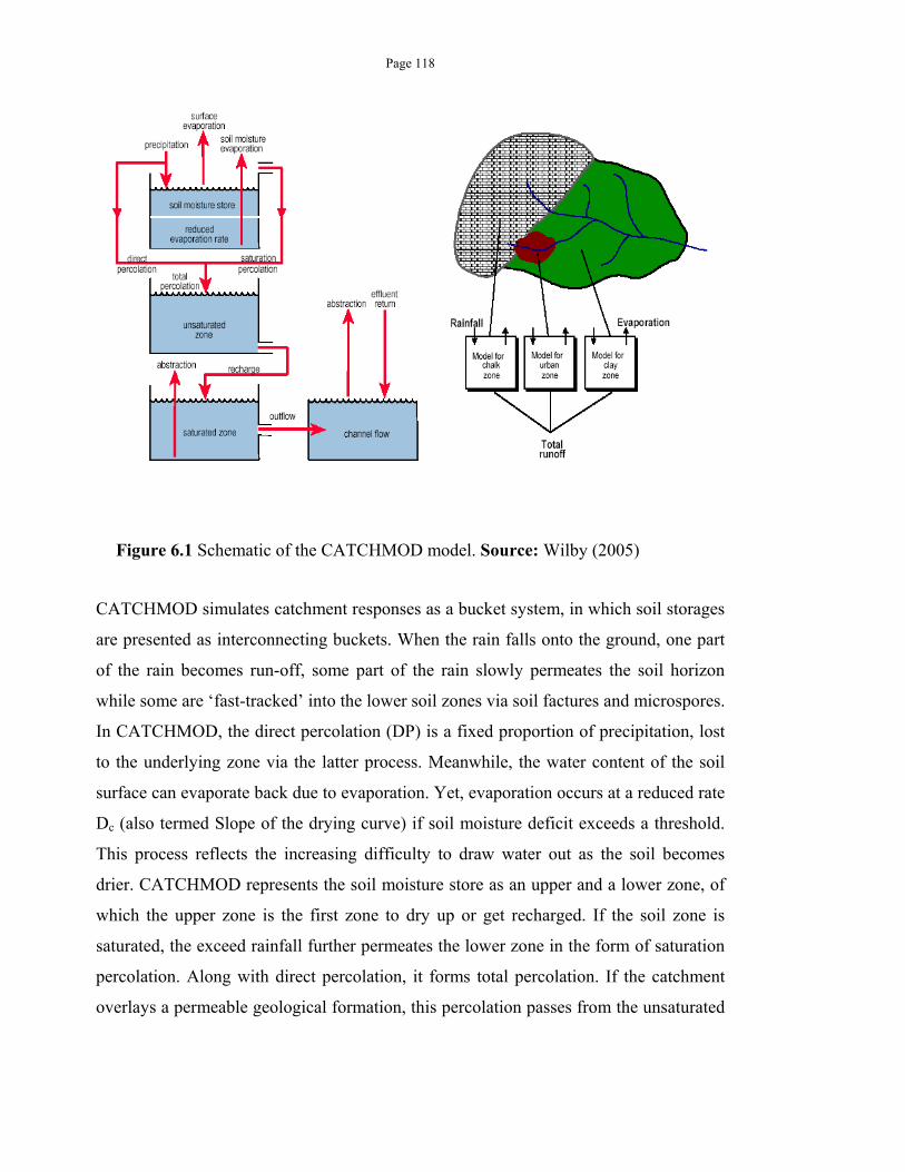
Page 118
Figure 6.1 Schematic of the CATCHMOD model. Source: Wilby (2005)
CATCHMOD simulates catchment responses as a bucket system, in which soil storages
are presented as interconnecting buckets. When the rain falls onto the ground, one part
of the rain becomes run-off, some part of the rain slowly permeates the soil horizon
while some are ‘fast-tracked’ into the lower soil zones via soil factures and microspores.
In CATCHMOD, the direct percolation (DP) is a fixed proportion of precipitation, lost
to the underlying zone via the latter process. Meanwhile, the water content of the soil
surface can evaporate back due to evaporation. Yet, evaporation occurs at a reduced rate
Dc (also termed Slope of the drying curve) if soil moisture deficit exceeds a threshold.
This process reflects the increasing difficulty to draw water out as the soil becomes
drier. CATCHMOD represents the soil moisture store as an upper and a lower zone, of
which the upper zone is the first zone to dry up or get recharged. If the soil zone is
saturated, the exceed rainfall further permeates the lower zone in the form of saturation
percolation. Along with direct percolation, it forms total percolation. If the catchment
overlays a permeable geological formation, this percolation passes from the unsaturated
Page 119
zone to the saturated zone and eventually becomes the base flow. This base flow is
released at a non-linear rate back to the flows. Apart from the natural hydrological
cycle, the water balance can be influenced by surface and groundwater abstraction, as
well as effluent return and discharge from irrigation. These influences are directly
subtracted or added at the relevant component, such as at the base flow or surface flow
calculation. For more information on model equation, please refer to Greenfield (1984),
Wilby et al. (1994) and Wilby and Harris (2006).
As such, there are two main differences of CATCHMOD flows compared to the SPEI
model. In CATCHMOD, when rainfall exceeds PET, this excess does not directly turn
into flows but some will be absorbed into the ground. While this process reduces the
direct runoff, it is partially offset by the subsurface and base flow contribution.
Therefore, a water balance model like CATCHMOD will have more ‘memory’ of the
previous catchment states than the SPEI model of the same time step resolution. For
instance, when PET is higher than rainfall, the SPEI model will result in no flows;
meanwhile, CATCHMOD can still simulate subsurface flows originating from the past
rainfall events.
In this study, this CATCHMOD model was chosen to represent the hydrological cycle
of the Rother Basin, which has been described in Chapter 4. The catchment model is
divided into six contributing areas representing the responses of different geological
structures. This setting is based on the VBA Excel-based CATCHMOD model used by
Southern Water and Atkins Consultants Ltd. Previous work of Southern Water and
Atkins have identified certain parameter sets that perform well under the calibration
period of 1990-1999 and the validation period of the 2000-2004 periods (Atkins Ltd.,
2009). Model performances were assessed using the Nash-Sutcliffe coefficient, the R2
and the mean squared residual of errors (MRSE). The Nash-Sutcliffe criterion is
essentially R2, but tends to -∞ when the total residual error of the observation and the
simulated values is worse than the total residual errors of the observations and their
Page 120
mean. Meanwhile R2 is a piecewise linear function that is identical to the Nash-Sutcliffe
coefficient in the positive zone and becomes 0 once the calculation returns negative
values. Hoang et al. (2012) reassessed these criteria and found that while these criteria
can indicate good model performance, each of these criteria orientates towards a
different model behaviour. For instance, a model with a small mean residual error tends
to have a good agreement in the large flows at the expense of the low flow errors, as an
error in the high flows is often much larger and affect the MSE more than a lower error
in the low flows. Meanwhile, the R2 criterion, the square of the correlation between the
observed flows and the simulated flows, tends to be more consistent in calibrating the
low flow and the high flow period since each residual error is scaled proportionally to
the observation. Nevertheless, both criteria are biased towards calibrating the high flow
periods, as a good performance in this region can still significantly compensate poor
performance elsewhere. In order to further enhance calibration in the low flow period,
the study additionally employs the Nash-Sutcliffe criterion of the base-10 logarithm of
the flows. For the purpose of the study, the VB.NET CATCHMOD model was
translated into the Fortran90 language, which gives a faster performance as required for
the number of runs. These VB.NET and Fortran90 versions were tested and yielded
similar results to the 6th significant number for flows in m3/s.
6.2.2. The GLUE methodology and Sobol sensitivity analysis
Uncertainty and sensitivity analysis are two closely intertwined fields. The former field
focuses on the uncertainty components of input data, the conceptual model and the
parameter values; the latter provides useful methodologies to analyse how the variations
in the model parameters can lead to changes in the outputs. In this study, two specific
methods of uncertainty and sensitivity analysis were combined to explore the
contribution of hydrological model parameterization to flow projections. Both of these
methodologies are Monte Carlo-based and require many model runs; an efficient
experimental design to conduct both of these analyses is therefore essential.
Page 121
6.2.2.1.The GLUE methodology
The Generalised Likelihood Uncertainty Estimation (GLUE) methodology (Beven and
Binley, 1992) uses a Monte Carlo sample of model parameters; it assumes the
likelihood of model acceptability to be equivalent to the goodness-of-fit measure. This
methodology emphasises that different model structures and parameterisation can
produce an acceptable model performance (equifinality). It thus moves away from the
traditional model calibration and validation process of selecting one optimal parameter
set towards a new framework. This framework uses an ensemble of model structures
and/or parameterization of satisfactory performance. The model ensemble is often
termed the ‘behavioural’ group and is selected based on a user-defined goodness-of-fit
threshold.
The outcome of GLUE is therefore several alternative representation of the catchment,
instead of an optimal parameter set such as the outcome of the classical model
validation process. The inclusion of several parameter sets thus is more likely to capture
the process under different conditions. For hydrological models, using GLUE produces
several parameter sets that capture the varying flow conditions, in contrast to the
dilemma of choosing an optimal parameter set; this is particularly beneficial if the
model parameter sets are not consistently optimal across different calibration periods or
criteria (Freer et al., 1996). Under a changing climate and hydrological regime, using
GLUE is valuable since the inclusion of more parameter sets might increase the
possibility of the model being able to perform despite these changes.
Yet, in such cases, the use of GLUE may also raise certain issues. Firstly, while distinct
parameter sets may produce converging results in the calibration period; under a
different time period and conditions, simulation results of such sets may diverge and
thus project different possibility of changes. If in the calibration period such differences
can be crosschecked with the observed flows, in the future there is not yet any data to
validate the ‘goodness-of-fit’ of these projections. While the variations in the GLUE
Page 122
projections, termed the ‘equifinality’ uncertainty (Beven and Freer, 2001; Beven, 2006),
are often assessed as a total term, there is a need to test whether distinct trends exist
within the overall equifinality uncertainty. Secondly, the future influence and the
interactions of the ‘behavioural’ parameter sets on the model outputs might be different
from the calibration period, thus affecting the overall likelihood of approximating the
true catchment behaviour. For instance, assuming a ‘behavioural’ CATCHMOD
parameter set was selected due to its capacity to simulate flows in intense convective
storms; the parameter set has a small direct percolation rate that is representative of the
soil condition in the calibration period. However if a drier condition would dominate the
future period, the soil then develops more cracks and macropores and thus facilitates
more direct percolation. As such, the parameter set is no longer representative of the
catchment conditions and will produce errors in the flow projections.
A closer inspection highlights a common issue of these two concerns. To date, many
principles in hydrology studies are based on the assumption of a single stable
equilibrium state, which the term ‘equifinality’ seems to suggest. This assumption is
evident in the common usage of a ‘warm-up’ period, in which a model is run for a
certain period to reduce the uncertainty due to different initial conditions. Yet, Peterson
et al. (2012) has shown that with the same parameter set, different initial conditions can
lead to multiple steady states in several hydrological systems. This thus demonstrates
the sensitivity of model and possibly catchment behaviour under different starting
conditions. In the case of the GLUE ensembles, considering that the ensemble consists
of different parameter sets, which subsequently produce different starting conditions in
each time step, these differences can cumulatively lead to totally different catchment
behaviours in the future projections. Furthermore, even within the calibration period,
their similar and ‘behavioural’ goodness-of-fit does not indicate that the sets represent
the same catchment response. Several works on GLUE (Wilby, 2005; Cloke et al.,
2012) have demonstrated that model performance changes seasonally, thus suggest that
some of the model is only representative of a certain condition and period. There
Page 123
subsequently exists a need to further inspect the group of ‘behavioural’ models to
analyse the alternative states that they represent.
6.2.2.2. Sobol Sensitivity Analysis
Consequently, it is essential to conduct sensitivity analysis in order to understand the
interactions and influence of the parameters on model performance and outputs. In the
calibration period, sensitivity analysis will contribute towards understanding how
different parameter sets converge to similar outcomes. For the future period, it provides
hints of which parameters may become more influential; additionally, knowledge of the
sensitive parameters will allow further monitoring of the changing conditions. Such
assessment may shed light on the possible causes and the implications of such changes.
In this study, the Sobol’s global sensitivity analysis method (Sobol', 1990; Sobol, 1993)
was chosen, with the scope of the analysis being the influence of a single parameter and
the combined influence of each parameter pairs. Similar to GLUE, Sobol is a global
sampling scheme to avoid oversampling around local minima or maxima. The Sobol
methodology assumes that the total variance of the model output is contributed by the
variance due to each single parameter (such as Vi, Vj, and Vk with i, j and k being the
corresponding parameters) and the interactions amongst the parameters (denoted Vij,
Vijk). Mathematically, if the input parameters are independent, this variance
decomposition can be presented as
Σ Σ Σ Σ Σ Σ ⋯ , ,…,
Equation 6.1
The Sobol Sensitivity indices are the ratio of the variance of each component and the
total variance. As such, dividing both sides by V, Equation 6.1 becomes
1 Σ Σ Σ Σ Σ Σ ⋯ , ,…,
Equation 6.2
The number of the parameters considered in each sensitivity index is termed the order
of the index. For instance, the first-order sensitivity index Si denotes the sensitivity of
Page 124
the output to changes in input i while the second-order Sij is the sensitivity due to the
interaction of input i and j. The total effect of a parameter i, the sum of all sensitivity
indices concerning i, is termed the total effect Ti. Often, these indices are not
analytically derived due to model complexity; the concerning indices are subsequently
approximated via a Monte Carlo sample of the model runs. To date, there have been
several proposed calculation methods, such as Saltelli (2002), Sobol et al. (2007) and
Jansen (1999). As the formulation varies, the specific required number of samples also
vary. The Sobol' (1990) scheme requires two equal-sized sets of independent samples
X1 and X2 in order to calculate the first-order indices. Assume that k parameters are
considered, each sample set will have the size of k x N with N being the sample size.
For a parameter i, the variance that i contributes to the model output can be estimated
by comparing model outputs of X1 and the same outputs when values of the parameter i
are replaced by the X2 values. While Saltelli et al. (2010) have summarised and
proposed a less computationally expensive sampling and calculation design, those
formulae only estimate the first and total sensitivity index. Therefore, in this study, the
classical Sobol’s method was selected. The study used the R sensitivity package (Pujol
et al., 2013) which includes the Sobol (1993)’s method. In order to enhance the sample,
the Latin Hypercube sampling technique was further used. This method ensures that the
sample is more evenly distributed across the equal-probability sampling grid (Saltelli et
al., 2000). In this study, parameter sampling and subsequent sensitivity analysis was
conducted using R while the model ran in Fortran90.
6.2.3. Experimental Design and Input Data
Model parameters: The sampling parameters include five soil moisture storage
parameters, two catchment storage parameters and two initial conditions of the
CATCHMOD model (Table 6-1).
6.2.2.3.Input data
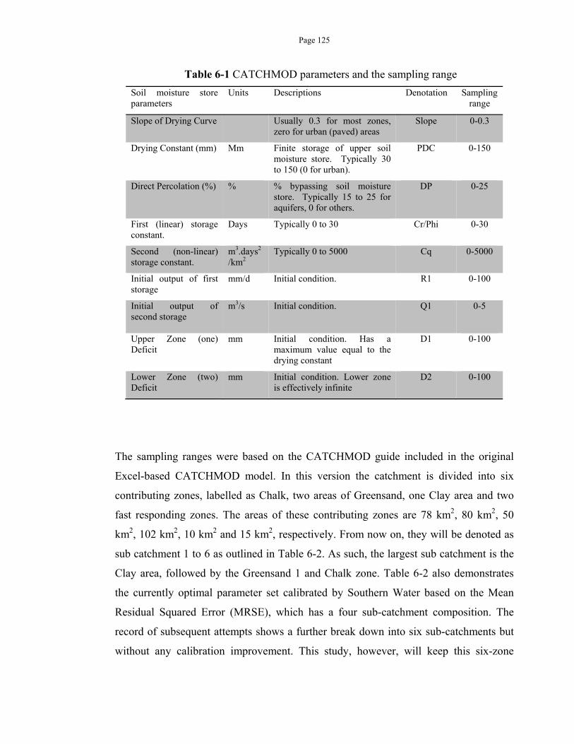
Page 125
Table 6-1 CATCHMOD parameters and the sampling range
Soil moisture store parameters
Units Descriptions Denotation Sampling range
Slope of Drying Curve Usually 0.3 for most zones, zero for urban (paved) areas
Slope 0-0.3
Drying Constant (mm) Mm Finite storage of upper soil moisture store. Typically 30 to 150 (0 for urban).
PDC 0-150
Direct Percolation (%) % % bypassing soil moisture store. Typically 15 to 25 for aquifers, 0 for others.
DP 0-25
First (linear) storage constant.
Days Typically 0 to 30 Cr/Phi 0-30
Second (non-linear) storage constant.
m3.days2
/km2 Typically 0 to 5000 Cq 0-5000
Initial output of first storage
mm/d Initial condition. R1 0-100
Initial output of second storage
m3/s Initial condition. Q1 0-5
Upper Zone (one) Deficit
mm Initial condition. Has a maximum value equal to the drying constant
D1 0-100
Lower Zone (two) Deficit
mm Initial condition. Lower zone is effectively infinite
D2 0-100
The sampling ranges were based on the CATCHMOD guide included in the original
Excel-based CATCHMOD model. In this version the catchment is divided into six
contributing zones, labelled as Chalk, two areas of Greensand, one Clay area and two
fast responding zones. The areas of these contributing zones are 78 km2, 80 km2, 50
km2, 102 km2, 10 km2 and 15 km2, respectively. From now on, they will be denoted as
sub catchment 1 to 6 as outlined in Table 6-2. As such, the largest sub catchment is the
Clay area, followed by the Greensand 1 and Chalk zone. Table 6-2 also demonstrates
the currently optimal parameter set calibrated by Southern Water based on the Mean
Residual Squared Error (MRSE), which has a four sub-catchment composition. The
record of subsequent attempts shows a further break down into six sub-catchments but
without any calibration improvement. This study, however, will keep this six-zone
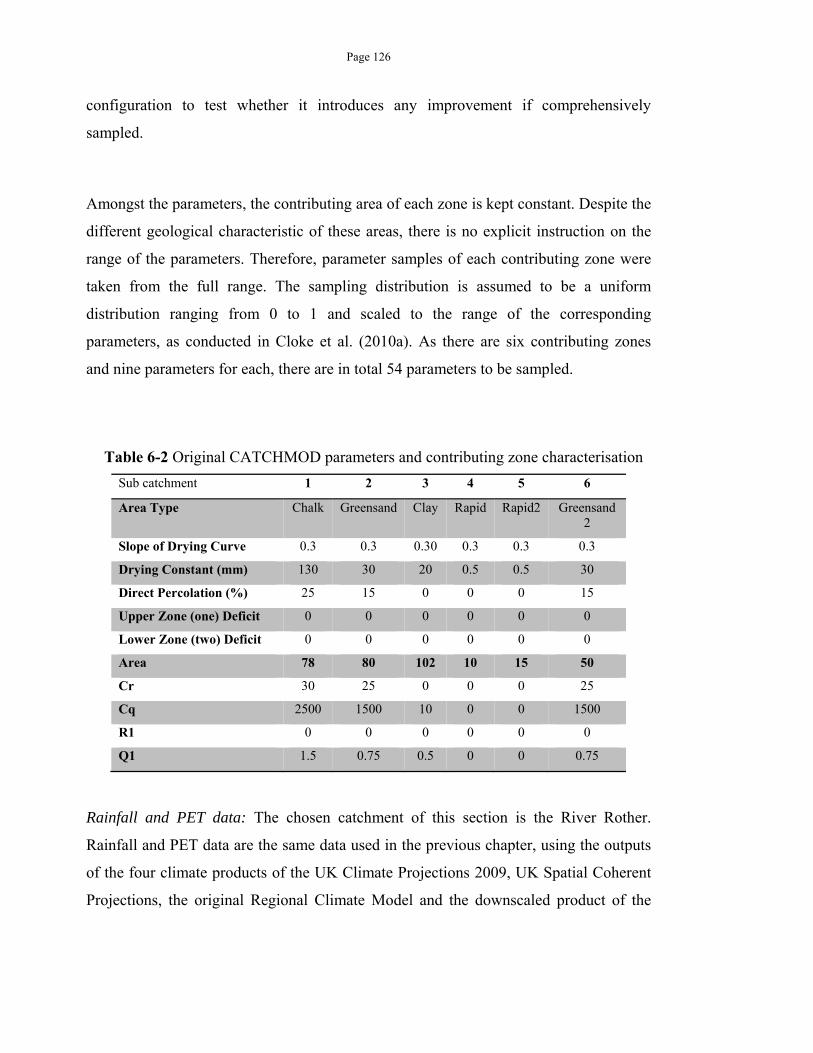
Page 126
configuration to test whether it introduces any improvement if comprehensively
sampled.
Amongst the parameters, the contributing area of each zone is kept constant. Despite the
different geological characteristic of these areas, there is no explicit instruction on the
range of the parameters. Therefore, parameter samples of each contributing zone were
taken from the full range. The sampling distribution is assumed to be a uniform
distribution ranging from 0 to 1 and scaled to the range of the corresponding
parameters, as conducted in Cloke et al. (2010a). As there are six contributing zones
and nine parameters for each, there are in total 54 parameters to be sampled.
Table 6-2 Original CATCHMOD parameters and contributing zone characterisation
Sub catchment 1 2 3 4 5 6
Area Type Chalk Greensand Clay Rapid Rapid2 Greensand 2
Slope of Drying Curve 0.3 0.3 0.30 0.3 0.3 0.3
Drying Constant (mm) 130 30 20 0.5 0.5 30
Direct Percolation (%) 25 15 0 0 0 15
Upper Zone (one) Deficit 0 0 0 0 0 0
Lower Zone (two) Deficit 0 0 0 0 0 0
Area 78 80 102 10 15 50
Cr 30 25 0 0 0 25
Cq 2500 1500 10 0 0 1500
R1 0 0 0 0 0 0
Q1 1.5 0.75 0.5 0 0 0.75
Rainfall and PET data: The chosen catchment of this section is the River Rother.
Rainfall and PET data are the same data used in the previous chapter, using the outputs
of the four climate products of the UK Climate Projections 2009, UK Spatial Coherent
Projections, the original Regional Climate Model and the downscaled product of the
Page 127
Future Flows Project. The assessed time periods are the historic period of 1961-1990,
the 2020s, 2030s and the 2050s.
6.2.2.4.Experimental design
The study uses two sampling sets to investigate the parameters
Sample 1-GLUE based analysis: 500,000 CATCHMOD runs using randomly
generated parameters were tested against two model settings: one with only one
contributing zone and another using the original structure of six contributing zones. The
purpose of this sampling scheme is to identify the ‘behavioural’ group of parameters
and conduct a preliminary assessment of parameter influences on model performance.
Sample 2-Sobol based analysis: 148,600 CATCHMOD parameter sets were
constructed from two Latin Hypercube sample sets X1 and X2. These 148,600 sets
enable the estimation of Sobol sensitivity indices up to the second order. Each set
consists of 100 sets of values for the 54 parameters. The Sobol test set was constructed
by iteratively replacing one or two vectors of X2 by the corresponding vectors of X1.
The comparison between model outputs of X1, X2 and the adjusted X2 can produce an
estimation of the first and second order sensitivity indices of each parameter. It should
be noted that this experimental design only enables an estimation of the indices. As
such, the larger number of samples contained in X1 and X2, the more reliable the
estimations are. Yet, due to time and computational constraints, the number of sampling
sets in X1 and X2 were kept at 100; the weak estimation power was partly compensated
by using the Latin hypercube sampling and 100 bootstrapping scheme. Yet, there is still
an uncertainty in these estimations.
Due to the large number of sets and computation constraints, it was not possible to run
either the 500,000 or 148,600 set on all the climate products. The Future Flows product
was thus chosen as the testing product of Sobol sensitivity indices. For all other sets, the
behavioural sets of Sample 1, which are less time and computational extensive than the
full 500,000 runs, were used.
Page 128
6.2.2.5.The efficiency criteria
In this study, the Nash-Sutcliffe coefficient of daily flows and the base 10 logarithm of
the daily flows were used. Additionally, the lowest total 7-day flows and the highest one
were also considered in order to further assess the influence of parameter values on the
flow projections.
In the historic period of both the GLUE and the Sobol experiment, the calibration
period is the 1990-2004 period. In the future period, as there is no historic flow, only
the lowest and the highest total 7-day flows are calculated over the whole period.
6.3.RESULTS AND DISCUSSION
6.3.1. The effect of soil storage on flows: Comparison of observation and SPEI
As previously discussed, SPEI is based on a simple water balance model of
precipitation subtracting potential evaporation. In reality, not all potential evaporation
can become actual evaporation. The catchment also responds more slowly than the
SPEI model, due to the effect of flow retention in soil storages. While not considering
the effect of soil storage, SPEI can have some ‘memory’ of previous month if calculated
on a longer period. As SPEI is calculated as a moving average over that period, the two-
month SPEI, for instance, can be affected by the rainfall-PET balance in the previous
month. Therefore, SPEI can reflect to a certain extent the retention effect, in a similar
manner that the autoregressive model considers the lagging effect of the past events.
Yet, that lagging effect is not uniform over the year. Figure 6.2 demonstrates that while
the correlation between SPEI and the actual flows are strong in the wet season, that
correlation is much weaker during the drier months of May to August.
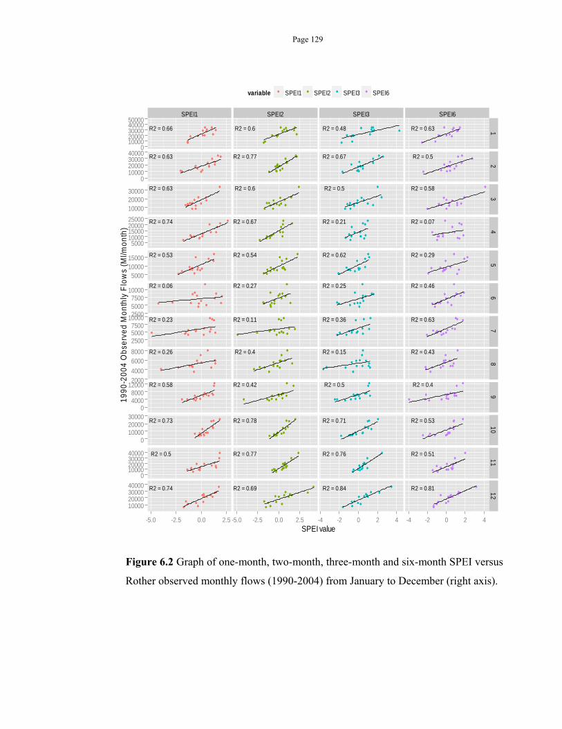
Page 129
Figure 6.2 Graph of one-month, two-month, three-month and six-month SPEI versus
Rother observed monthly flows (1990-2004) from January to December (right axis).
SPEI1 SPEI2 SPEI3 SPEI6
R2 = 0.66
R2 = 0.63
R2 = 0.63
R2 = 0.74
R2 = 0.53
R2 = 0.06
R2 = 0.23
R2 = 0.26
R2 = 0.58
R2 = 0.73
R2 = 0.5
R2 = 0.74
R2 = 0.6
R2 = 0.77
R2 = 0.6
R2 = 0.67
R2 = 0.54
R2 = 0.27
R2 = 0.11
R2 = 0.4
R2 = 0.42
R2 = 0.78
R2 = 0.77
R2 = 0.69
R2 = 0.48
R2 = 0.67
R2 = 0.5
R2 = 0.21
R2 = 0.62
R2 = 0.25
R2 = 0.36
R2 = 0.15
R2 = 0.5
R2 = 0.71
R2 = 0.76
R2 = 0.84
R2 = 0.63
R2 = 0.5
R2 = 0.58
R2 = 0.07
R2 = 0.29
R2 = 0.46
R2 = 0.63
R2 = 0.43
R2 = 0.4
R2 = 0.53
R2 = 0.51
R2 = 0.81
01000020000300004000050000
010000200003000040000
100002000030000
500010000150002000025000
50001000015000
250050007500
10000
250050007500
10000
20004000
60008000
040008000
12000
0100002000030000
010000200003000040000
10000200003000040000
12
34
56
78
910
1112
-5.0 -2.5 0.0 2.5 -5.0 -2.5 0.0 2.5 -4 -2 0 2 4 -4 -2 0 2 4SPEI value
199
0-2
00
4 O
bse
rve
d M
on
thly
Flo
ws
(Ml/m
onth
)
variable SPEI1 SPEI2 SPEI3 SPEI6
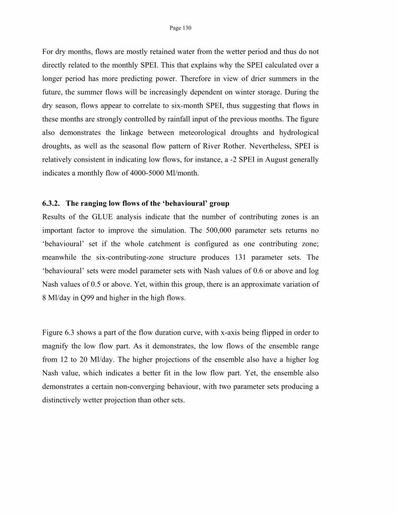
Page 130
For dry months, flows are mostly retained water from the wetter period and thus do not
directly related to the monthly SPEI. This that explains why the SPEI calculated over a
longer period has more predicting power. Therefore in view of drier summers in the
future, the summer flows will be increasingly dependent on winter storage. During the
dry season, flows appear to correlate to six-month SPEI, thus suggesting that flows in
these months are strongly controlled by rainfall input of the previous months. The figure
also demonstrates the linkage between meteorological droughts and hydrological
droughts, as well as the seasonal flow pattern of River Rother. Nevertheless, SPEI is
relatively consistent in indicating low flows, for instance, a -2 SPEI in August generally
indicates a monthly flow of 4000-5000 Ml/month.
6.3.2. The ranging low flows of the ‘behavioural’ group
Results of the GLUE analysis indicate that the number of contributing zones is an
important factor to improve the simulation. The 500,000 parameter sets returns no
‘behavioural’ set if the whole catchment is configured as one contributing zone;
meanwhile the six-contributing-zone structure produces 131 parameter sets. The
‘behavioural’ sets were model parameter sets with Nash values of 0.6 or above and log
Nash values of 0.5 or above. Yet, within this group, there is an approximate variation of
8 Ml/day in Q99 and higher in the high flows.
Figure 6.3 shows a part of the flow duration curve, with x-axis being flipped in order to
magnify the low flow part. As it demonstrates, the low flows of the ensemble range
from 12 to 20 Ml/day. The higher projections of the ensemble also have a higher log
Nash value, which indicates a better fit in the low flow part. Yet, the ensemble also
demonstrates a certain non-converging behaviour, with two parameter sets producing a
distinctively wetter projection than other sets.
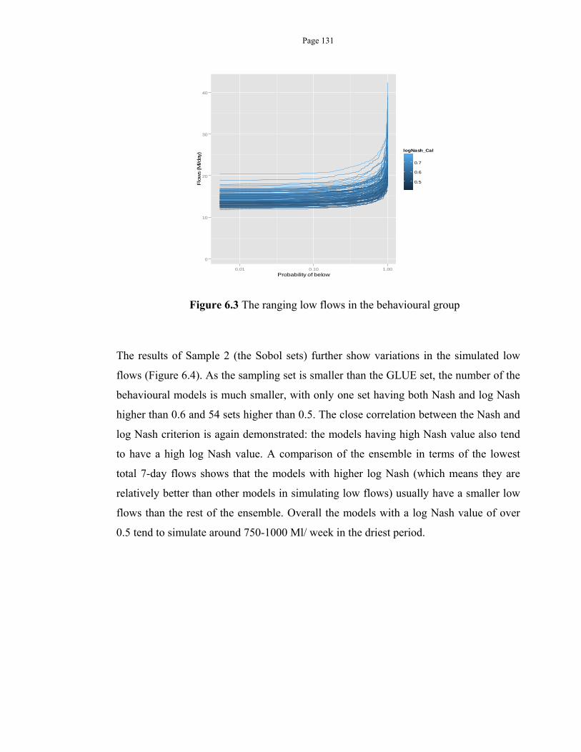
Page 131
Figure 6.3 The ranging low flows in the behavioural group
The results of Sample 2 (the Sobol sets) further show variations in the simulated low
flows (Figure 6.4). As the sampling set is smaller than the GLUE set, the number of the
behavioural models is much smaller, with only one set having both Nash and log Nash
higher than 0.6 and 54 sets higher than 0.5. The close correlation between the Nash and
log Nash criterion is again demonstrated: the models having high Nash value also tend
to have a high log Nash value. A comparison of the ensemble in terms of the lowest
total 7-day flows shows that the models with higher log Nash (which means they are
relatively better than other models in simulating low flows) usually have a smaller low
flows than the rest of the ensemble. Overall the models with a log Nash value of over
0.5 tend to simulate around 750-1000 Ml/ week in the driest period.
0
10
20
30
40
0.01 0.10 1.00Probability of below
Flo
ws
(Ml/d
ay)
0.5
0.6
0.7
logNash_Cal
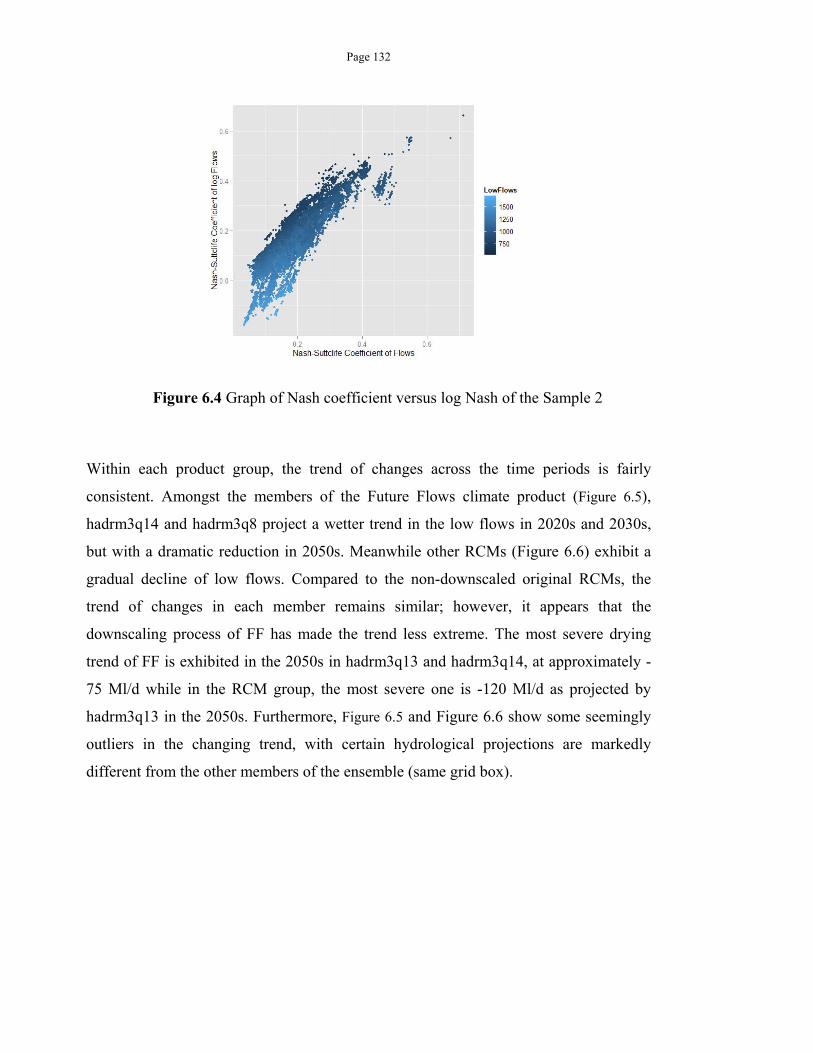
Page 132
Figure 6.4 Graph of Nash coefficient versus log Nash of the Sample 2
Within each product group, the trend of changes across the time periods is fairly
consistent. Amongst the members of the Future Flows climate product (Figure 6.5),
hadrm3q14 and hadrm3q8 project a wetter trend in the low flows in 2020s and 2030s,
but with a dramatic reduction in 2050s. Meanwhile other RCMs (Figure 6.6) exhibit a
gradual decline of low flows. Compared to the non-downscaled original RCMs, the
trend of changes in each member remains similar; however, it appears that the
downscaling process of FF has made the trend less extreme. The most severe drying
trend of FF is exhibited in the 2050s in hadrm3q13 and hadrm3q14, at approximately -
75 Ml/d while in the RCM group, the most severe one is -120 Ml/d as projected by
hadrm3q13 in the 2050s. Furthermore, Figure 6.5 and Figure 6.6 show some seemingly
outliers in the changing trend, with certain hydrological projections are markedly
different from the other members of the ensemble (same grid box).
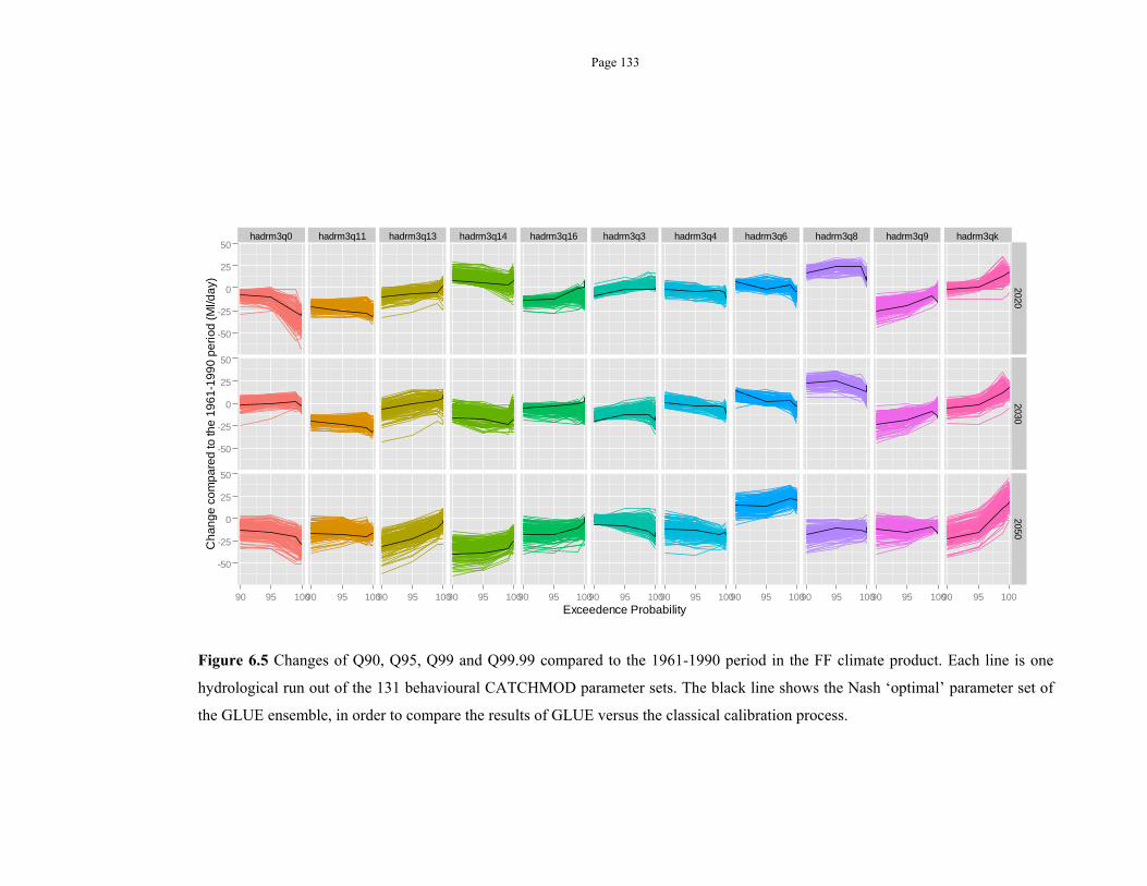
Page 133
Figure 6.5 Changes of Q90, Q95, Q99 and Q99.99 compared to the 1961-1990 period in the FF climate product. Each line is one
hydrological run out of the 131 behavioural CATCHMOD parameter sets. The black line shows the Nash ‘optimal’ parameter set of
the GLUE ensemble, in order to compare the results of GLUE versus the classical calibration process.
hadrm3q0 hadrm3q11 hadrm3q13 hadrm3q14 hadrm3q16 hadrm3q3 hadrm3q4 hadrm3q6 hadrm3q8 hadrm3q9 hadrm3qk
-50
-25
0
25
50
-50
-25
0
25
50
-50
-25
0
25
50
20202030
2050
90 95 10090 95 10090 95 10090 95 10090 95 10090 95 10090 95 10090 95 10090 95 10090 95 10090 95 100Exceedence Probability
Ch
ang
e c
om
pa
red
to th
e 19
61
-19
90
pe
riod
(M
l/da
y)
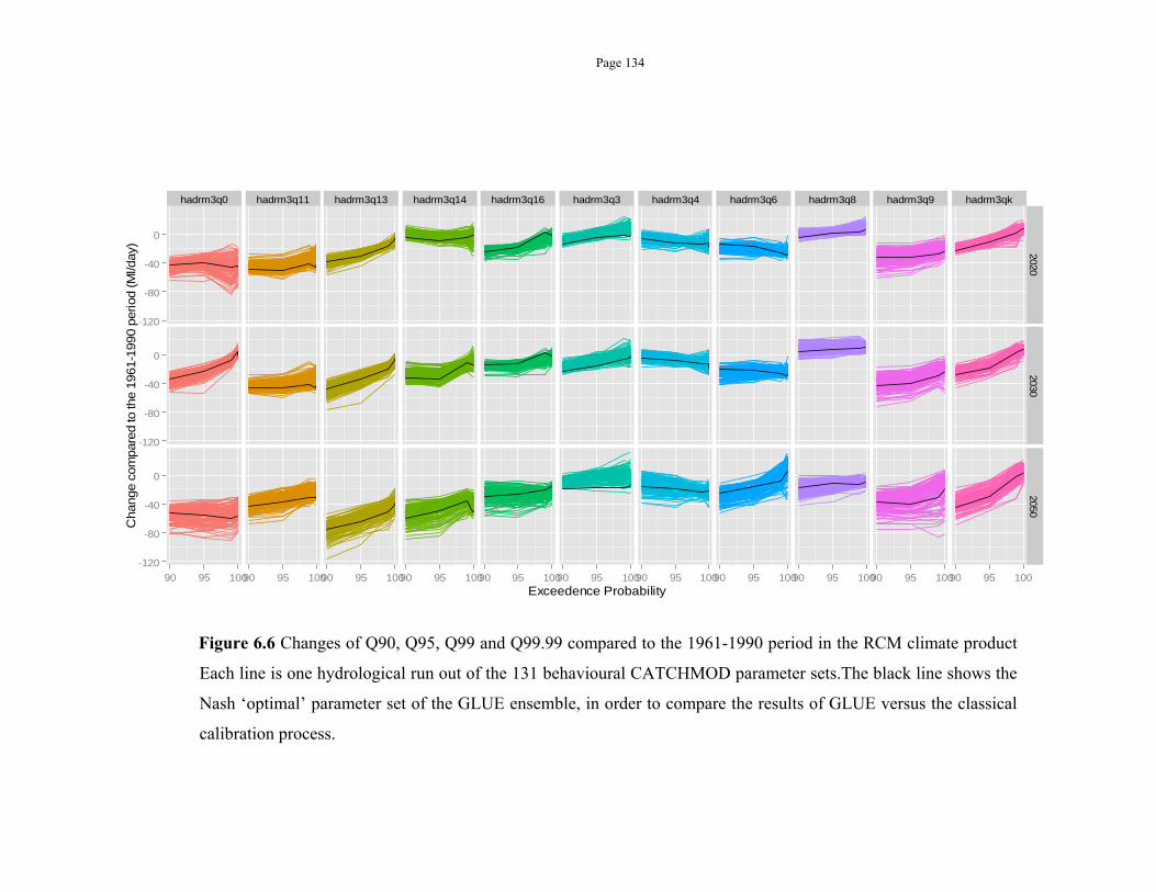
Page 134
Figure 6.6 Changes of Q90, Q95, Q99 and Q99.99 compared to the 1961-1990 period in the RCM climate product
Each line is one hydrological run out of the 131 behavioural CATCHMOD parameter sets.The black line shows the
Nash ‘optimal’ parameter set of the GLUE ensemble, in order to compare the results of GLUE versus the classical
calibration process.
hadrm3q0 hadrm3q11 hadrm3q13 hadrm3q14 hadrm3q16 hadrm3q3 hadrm3q4 hadrm3q6 hadrm3q8 hadrm3q9 hadrm3qk
-120
-80
-40
0
-120
-80
-40
0
-120
-80
-40
0
20202030
2050
90 95 10090 95 10090 95 10090 95 10090 95 10090 95 10090 95 10090 95 10090 95 10090 95 10090 95 100Exceedence Probability
Change c
om
par
ed to
the 1
961-1
990 p
eriod
(M
l/day)
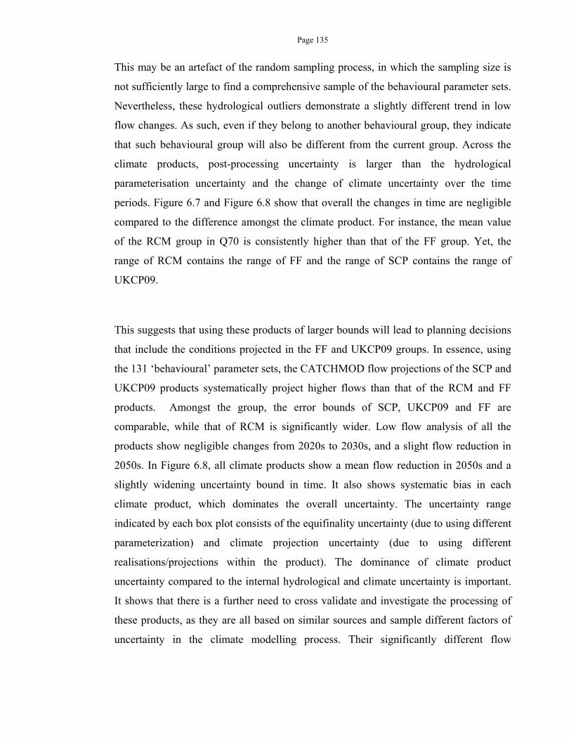
Page 135
This may be an artefact of the random sampling process, in which the sampling size is
not sufficiently large to find a comprehensive sample of the behavioural parameter sets.
Nevertheless, these hydrological outliers demonstrate a slightly different trend in low
flow changes. As such, even if they belong to another behavioural group, they indicate
that such behavioural group will also be different from the current group. Across the
climate products, post-processing uncertainty is larger than the hydrological
parameterisation uncertainty and the change of climate uncertainty over the time
periods. Figure 6.7 and Figure 6.8 show that overall the changes in time are negligible
compared to the difference amongst the climate product. For instance, the mean value
of the RCM group in Q70 is consistently higher than that of the FF group. Yet, the
range of RCM contains the range of FF and the range of SCP contains the range of
UKCP09.
This suggests that using these products of larger bounds will lead to planning decisions
that include the conditions projected in the FF and UKCP09 groups. In essence, using
the 131 ‘behavioural’ parameter sets, the CATCHMOD flow projections of the SCP and
UKCP09 products systematically project higher flows than that of the RCM and FF
products. Amongst the group, the error bounds of SCP, UKCP09 and FF are
comparable, while that of RCM is significantly wider. Low flow analysis of all the
products show negligible changes from 2020s to 2030s, and a slight flow reduction in
2050s. In Figure 6.8, all climate products show a mean flow reduction in 2050s and a
slightly widening uncertainty bound in time. It also shows systematic bias in each
climate product, which dominates the overall uncertainty. The uncertainty range
indicated by each box plot consists of the equifinality uncertainty (due to using different
parameterization) and climate projection uncertainty (due to using different
realisations/projections within the product). The dominance of climate product
uncertainty compared to the internal hydrological and climate uncertainty is important.
It shows that there is a further need to cross validate and investigate the processing of
these products, as they are all based on similar sources and sample different factors of
uncertainty in the climate modelling process. Their significantly different flow

Page 136
projections imply that such uncertainty may further cascade down the modelling
process and may lead to different adaptation and planning decision depending on which
climate product is employed. To date, all of these products have been used in adaptation
studies, with the SCP and UKCP09 being used for water resource plans in England and
Wales, the RCM being used for several climate change research studies and the FF
projections used to assess climate risks in key catchments.
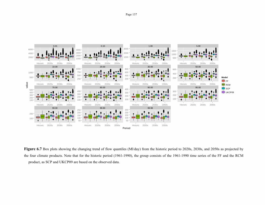
Page 137
Figure 6.7 Box plots showing the changing trend of flow quantiles (Ml/day) from the historic period to 2020s, 2030s, and 2050s as projected by
the four climate products. Note that for the historic period (1961-1990), the group consists of the 1961-1990 time series of the FF and the RCM
product, as SCP and UKCP09 are based on the observed data.
0.01 0.10 1.00 5.00
10.00 20.00 30.00 50.00
70.00 80.00 90.00 95.00
99.00 99.90 99.98
2000
4000
6000
1000200030004000
1000
2000
3000
500
1000
1500
500
1000
250
500
750
1000
200
400
600
800
200
400
600
100200300400500
100200300400
100
200
300
400
100
200
300
100
200
50100150200250
50100150200250
Historic 2020s 2030s 2050s Historic 2020s 2030s 2050s Historic 2020s 2030s 2050s Historic 2020s 2030s 2050s
Historic 2020s 2030s 2050s Historic 2020s 2030s 2050s Historic 2020s 2030s 2050s Historic 2020s 2030s 2050s
Historic 2020s 2030s 2050s Historic 2020s 2030s 2050s Historic 2020s 2030s 2050s Historic 2020s 2030s 2050s
Historic 2020s 2030s 2050s Historic 2020s 2030s 2050s Historic 2020s 2030s 2050sPeriod
valu
e
Model
FF
RCM
SCP
UKCP09
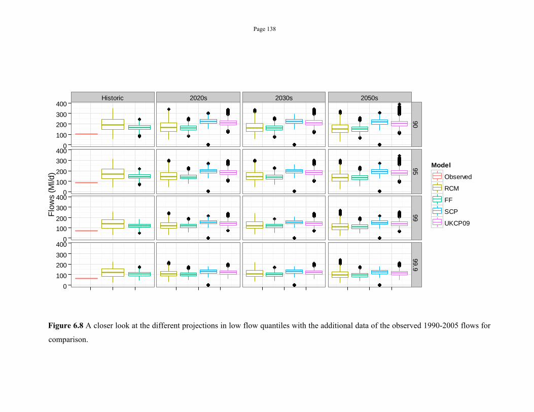
Page 138
Figure 6.8 A closer look at the different projections in low flow quantiles with the additional data of the observed 1990-2005 flows for
comparison.
Historic 2020s 2030s 2050s
0
100
200
300
400
0
100
200
300
400
0
100
200
300
400
0
100
200
300
400
9095
9999.9
1
Flo
ws
(Ml/d
)
Model
Observed
RCM
FF
SCP
UKCP09
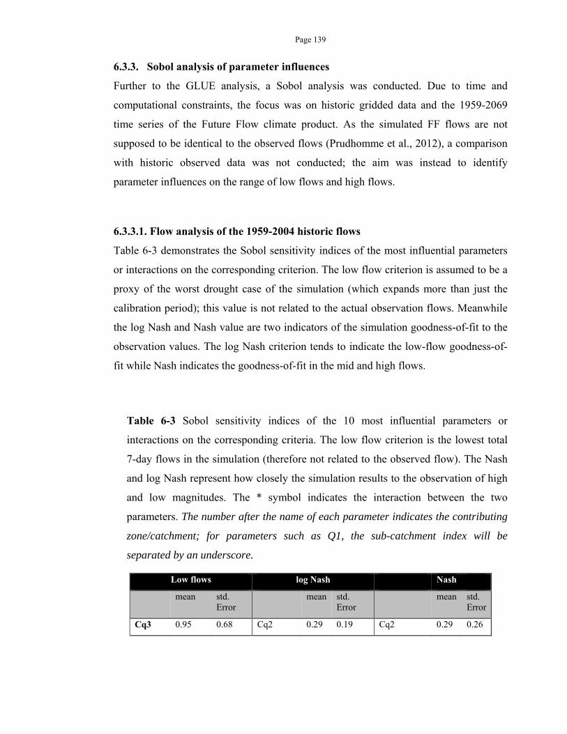
Page 139
6.3.3. Sobol analysis of parameter influences
Further to the GLUE analysis, a Sobol analysis was conducted. Due to time and
computational constraints, the focus was on historic gridded data and the 1959-2069
time series of the Future Flow climate product. As the simulated FF flows are not
supposed to be identical to the observed flows (Prudhomme et al., 2012), a comparison
with historic observed data was not conducted; the aim was instead to identify
parameter influences on the range of low flows and high flows.
6.3.3.1. Flow analysis of the 1959-2004 historic flows
Table 6-3 demonstrates the Sobol sensitivity indices of the most influential parameters
or interactions on the corresponding criterion. The low flow criterion is assumed to be a
proxy of the worst drought case of the simulation (which expands more than just the
calibration period); this value is not related to the actual observation flows. Meanwhile
the log Nash and Nash value are two indicators of the simulation goodness-of-fit to the
observation values. The log Nash criterion tends to indicate the low-flow goodness-of-
fit while Nash indicates the goodness-of-fit in the mid and high flows.
Table 6-3 Sobol sensitivity indices of the 10 most influential parameters or
interactions on the corresponding criteria. The low flow criterion is the lowest total
7-day flows in the simulation (therefore not related to the observed flow). The Nash
and log Nash represent how closely the simulation results to the observation of high
and low magnitudes. The * symbol indicates the interaction between the two
parameters. The number after the name of each parameter indicates the contributing
zone/catchment; for parameters such as Q1, the sub-catchment index will be
separated by an underscore.
Low flows log Nash Nash
mean std. Error
mean std. Error
mean std. Error
Cq3 0.95 0.68 Cq2 0.29 0.19 Cq2 0.29 0.26

Page 140
Cq1 0.86 0.96 Cq3 0.22 0.23 Phi2*Cq2 0.23 0.46
Cq2 0.86 0.92 Cq1 0.18 0.21 Phi1*Cq1 0.22 0.32
Cq6 0.74 0.93 Cq6 0.08 0.20 Cq3 0.14 0.41
Slope1 0.70 1.03 Phi1*Cq1 0.07 0.21 Cq1*Cq2 0.08 0.33
Pdc1 0.70 1.01 Phi6 0.06 0.20 Cq1*Cq3 0.07 0.35
Pdc6 0.69 1.03 Pdc3 0.05 0.19 Cq2*Cq6 0.07 0.35
Pdc3 0.69 0.96 Phi1 0.05 0.19 Phi2 0.07 0.32
Phi2 0.68 1.01 Phi2 0.04 0.20 Pdc6*Cq6 0.06 0.34
Cq5 0.67 1.00 Cq4 0.03 0.19 Slope6*Cq6 0.06 0.33
6.3.3.2.Low flow indicators
Analysis on the historic flows of 1959-2004 show that both the lowest total 7-day flows
and the log Nash value are strongly controlled by the non-linear storage constant of the
1st, 2nd and the 3rd contributing zone, the three largest zones of the catchment (Figure 6.9
and Figure 9.10). The figures show a positive relation between Cq and 7-day low flows
and a negative relation between Cq and log-Nash. Therefore, the higher Cq is, the
wetter the simulation is. As the actual driest flow in the catchment tends toward the dry
case of approximate 700-1000 Ml/week, small Cq values lead to a better low flow fit.
The dominance of Cq during the low flow periods can be explained by the soil function
that the parameter represents: the base flow release rate. Low flows often occur in
prolonged periods of limited rainfall and/or excessive evaporation. In such
circumstances, the upper soil storage and the unsaturated zone are often dry and can
contribute little to the underlying storages. This thus explains the limited role of the
parameters representing those processes. On the contrary, base flow is a significant
contributor to river flows when other sources wane. As the correlation analysis between
SPEI and observed flows has shown, flows in the dry period are weakly dependent on
the actual rainfall and PET balance of that month. During these periods, flows rely on
soil storages, which were accumulated in the previous rainfall events. As such, a model

Page 141
with a larger value of Cq, implying a higher releasing rate, will contribute to higher
flows. Furthermore, Cq is the releasing rate per km2; consequently, the total release
volume would be the product of the unit releasing rate and the area of the contributing
zone. As such, sub catchment area and the value of Cq are two important factors
deciding the overall flows. This influence is evident in
Figure 6.10, in which low flows increase when the value of Cq increases, particularly in
the large sub-catchment. The controlling role of Cq on log Nash value also indicates
that this is an important parameter in calibrating low flows.
Figure 6.9 Graph of the standardized Cq versus the lowest total 7-day flows in six contributing zones. As can be seen, Cq3 shows a less noisy correlation between the low flows and the Cq3 value.
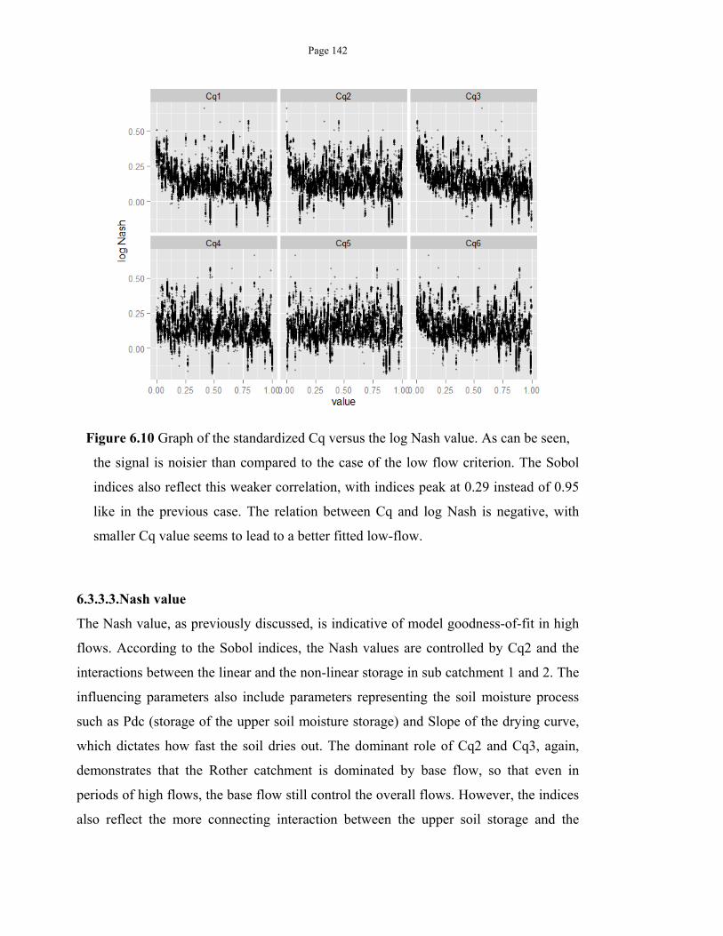
Page 142
Figure 6.10 Graph of the standardized Cq versus the log Nash value. As can be seen,
the signal is noisier than compared to the case of the low flow criterion. The Sobol
indices also reflect this weaker correlation, with indices peak at 0.29 instead of 0.95
like in the previous case. The relation between Cq and log Nash is negative, with
smaller Cq value seems to lead to a better fitted low-flow.
6.3.3.3.Nash value
The Nash value, as previously discussed, is indicative of model goodness-of-fit in high
flows. According to the Sobol indices, the Nash values are controlled by Cq2 and the
interactions between the linear and the non-linear storage in sub catchment 1 and 2. The
influencing parameters also include parameters representing the soil moisture process
such as Pdc (storage of the upper soil moisture storage) and Slope of the drying curve,
which dictates how fast the soil dries out. The dominant role of Cq2 and Cq3, again,
demonstrates that the Rother catchment is dominated by base flow, so that even in
periods of high flows, the base flow still control the overall flows. However, the indices
also reflect the more connecting interaction between the upper soil storage and the
Page 143
underlying storages in such wet periods. In essence, the influence of Cq2 and Phi2, the
unsaturated zone that receives percolation from the soil moisture store and direct
rainfall, shows the direct contribution of rainfall events. The analysis also implies the
need to obtain both acceptable Phi and Cq values, as well as a well-fitted Cq values
across the contributing zones in order to correctly reflect the catchment processes in
high flows. Figure 6.11 shows that while the Cq2 and Phi2 interaction has a strong
influence on the Nash criterion, that influence is not monotonous. As can be seen, there
are pockets of local minima and maxima. This further affirms the need to conduct a
global sampling on the parameter sets, since acceptable parameter combinations can
exist in various place in the sampling space.
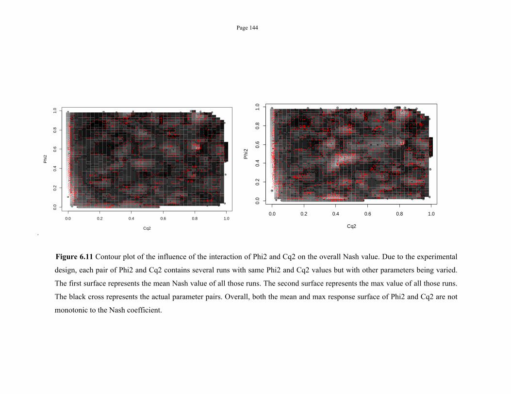
Page 144
.
Figure 6.11 Contour plot of the influence of the interaction of Phi2 and Cq2 on the overall Nash value. Due to the experimental
design, each pair of Phi2 and Cq2 contains several runs with same Phi2 and Cq2 values but with other parameters being varied.
The first surface represents the mean Nash value of all those runs. The second surface represents the max value of all those runs.
The black cross represents the actual parameter pairs. Overall, both the mean and max response surface of Phi2 and Cq2 are not
monotonic to the Nash coefficient.
0.0 0.2 0.4 0.6 0.8 1.0
0.0
0.2
0.4
0.6
0.8
1.0
Cq2
Ph
i2
0.0 0.2 0.4 0.6 0.8 1.0
0.0
0.2
0.4
0.6
0.8
1.0
Cq2
Ph
i2
Page 145
6.3.3.4.The influence of the initial conditions
Regarding the influence of the initial conditions on the simulation, Table 6-3 Sobol
sensitivity indices of the 10 most influential parameters or interactions on the
corresponding criteria. does not indicate any initial condition parameters as an
influencing factor. Upon a close inspection of the whole parameter list, the initial
condition parameter D1, Q1 and R1 appear to have certain influence on the 7-day low
flows but not on the criteria of log Nash and Nash. This can be explained by the
difference between the two groups of criteria. In the case of log Nash and Nash,
regardless of the initial conditions, there likely exists a parameter set that can
compensate the dryness or wetness of the initial conditions and slowly mitigate the
effect. Furthermore, the calibration period is from 1990 to 2004, while the model starts
from 1959. Over time, the effect of the initial conditions are likely to be dampened by
the influence of other parameters; however if the calibration period has been closer to
the starting time step, the influence of the initial conditions will grow. Meanwhile, the
low flow period can occur in any time step of the simulation. Therefore, while the initial
conditions are not the dominant factor, drier initial conditions once coupled with small
catchment storage can lead to a lower 7-day flow than in the case of wetter initial
conditions.
6.3.4. Future Flows analysis on parameter influences
6.3.4.1.Low flows
In the FF climate product, the non-linear storage constant Cq of catchment 1 and 3, the
slope of drying curve of catchment 1 and the linear storage constant Pdc of the
catchments are among the ten most influential factors on low flow simulation (Table
6-4).
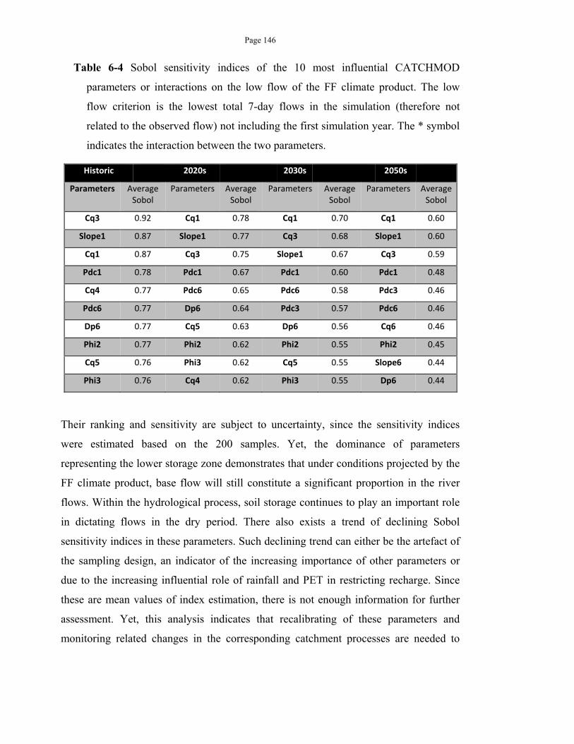
Page 146
Table 6-4 Sobol sensitivity indices of the 10 most influential CATCHMOD
parameters or interactions on the low flow of the FF climate product. The low
flow criterion is the lowest total 7-day flows in the simulation (therefore not
related to the observed flow) not including the first simulation year. The * symbol
indicates the interaction between the two parameters.
Historic 2020s 2030s 2050s
Parameters Average Sobol
Parameters Average Sobol
Parameters Average Sobol
Parameters Average Sobol
Cq3 0.92 Cq1 0.78 Cq1 0.70 Cq1 0.60
Slope1 0.87 Slope1 0.77 Cq3 0.68 Slope1 0.60
Cq1 0.87 Cq3 0.75 Slope1 0.67 Cq3 0.59
Pdc1 0.78 Pdc1 0.67 Pdc1 0.60 Pdc1 0.48
Cq4 0.77 Pdc6 0.65 Pdc6 0.58 Pdc3 0.46
Pdc6 0.77 Dp6 0.64 Pdc3 0.57 Pdc6 0.46
Dp6 0.77 Cq5 0.63 Dp6 0.56 Cq6 0.46
Phi2 0.77 Phi2 0.62 Phi2 0.55 Phi2 0.45
Cq5 0.76 Phi3 0.62 Cq5 0.55 Slope6 0.44
Phi3 0.76 Cq4 0.62 Phi3 0.55 Dp6 0.44
Their ranking and sensitivity are subject to uncertainty, since the sensitivity indices
were estimated based on the 200 samples. Yet, the dominance of parameters
representing the lower storage zone demonstrates that under conditions projected by the
FF climate product, base flow will still constitute a significant proportion in the river
flows. Within the hydrological process, soil storage continues to play an important role
in dictating flows in the dry period. There also exists a trend of declining Sobol
sensitivity indices in these parameters. Such declining trend can either be the artefact of
the sampling design, an indicator of the increasing importance of other parameters or
due to the increasing influential role of rainfall and PET in restricting recharge. Since
these are mean values of index estimation, there is not enough information for further
assessment. Yet, this analysis indicates that recalibrating of these parameters and
monitoring related changes in the corresponding catchment processes are needed to
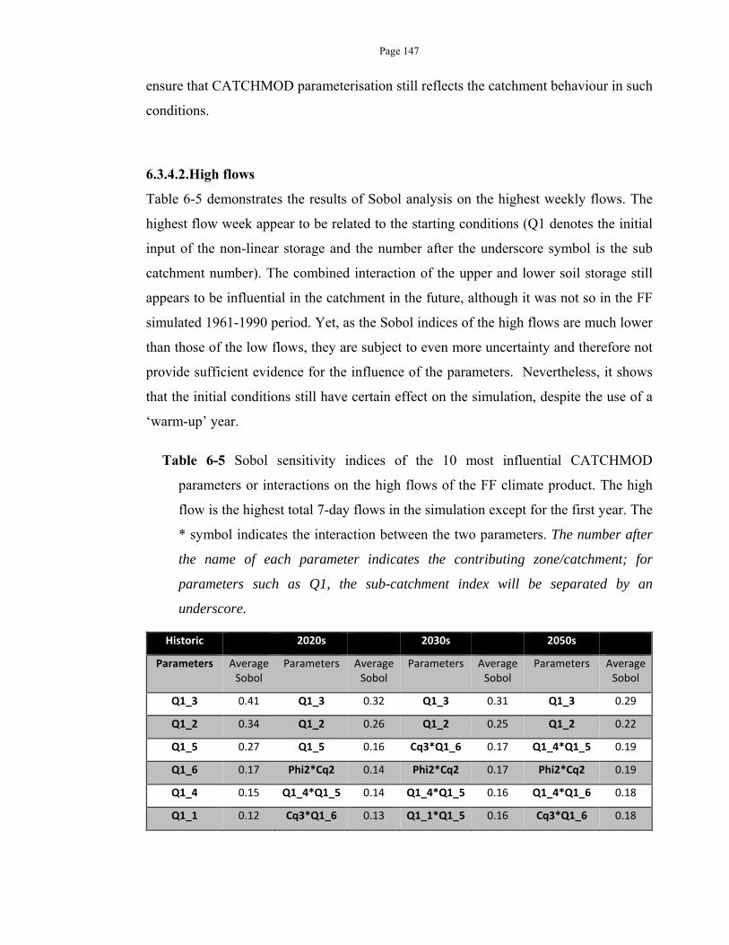
Page 147
ensure that CATCHMOD parameterisation still reflects the catchment behaviour in such
conditions.
6.3.4.2.High flows
Table 6-5 demonstrates the results of Sobol analysis on the highest weekly flows. The
highest flow week appear to be related to the starting conditions (Q1 denotes the initial
input of the non-linear storage and the number after the underscore symbol is the sub
catchment number). The combined interaction of the upper and lower soil storage still
appears to be influential in the catchment in the future, although it was not so in the FF
simulated 1961-1990 period. Yet, as the Sobol indices of the high flows are much lower
than those of the low flows, they are subject to even more uncertainty and therefore not
provide sufficient evidence for the influence of the parameters. Nevertheless, it shows
that the initial conditions still have certain effect on the simulation, despite the use of a
‘warm-up’ year.
Table 6-5 Sobol sensitivity indices of the 10 most influential CATCHMOD
parameters or interactions on the high flows of the FF climate product. The high
flow is the highest total 7-day flows in the simulation except for the first year. The
* symbol indicates the interaction between the two parameters. The number after
the name of each parameter indicates the contributing zone/catchment; for
parameters such as Q1, the sub-catchment index will be separated by an
underscore.
Historic 2020s 2030s 2050s
Parameters Average Sobol
Parameters Average Sobol
Parameters Average Sobol
Parameters Average Sobol
Q1_3 0.41 Q1_3 0.32 Q1_3 0.31 Q1_3 0.29
Q1_2 0.34 Q1_2 0.26 Q1_2 0.25 Q1_2 0.22
Q1_5 0.27 Q1_5 0.16 Cq3*Q1_6 0.17 Q1_4*Q1_5 0.19
Q1_6 0.17 Phi2*Cq2 0.14 Phi2*Cq2 0.17 Phi2*Cq2 0.19
Q1_4 0.15 Q1_4*Q1_5 0.14 Q1_4*Q1_5 0.16 Q1_4*Q1_6 0.18
Q1_1 0.12 Cq3*Q1_6 0.13 Q1_1*Q1_5 0.16 Cq3*Q1_6 0.18
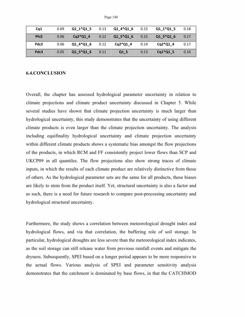
Page 148
Cq1 0.09 Q1_1*Q1_5 0.13 Q1_4*Q1_6 0.15 Q1_1*Q1_5 0.18
Phi2 0.06 Cq2*Q1_4 0.12 Q1_5*Q1_6 0.15 Q1_5*Q1_6 0.17
Pdc2 0.06 Q1_4*Q1_6 0.12 Cq2*Q1_4 0.14 Cq2*Q1_4 0.17
Pdc3 0.05 Q1_5*Q1_6 0.11 Q1_5 0.13 Cq1*Q1_5 0.16
6.4.CONCLUSION
Overall, the chapter has assessed hydrological parameter uncertainty in relation to
climate projections and climate product uncertainty discussed in Chapter 5. While
several studies have shown that climate projection uncertainty is much larger than
hydrological uncertainty, this study demonstrates that the uncertainty of using different
climate products is even larger than the climate projection uncertainty. The analysis
including equifinality hydrological uncertainty and climate projection uncertainty
within different climate products shows a systematic bias amongst the flow projections
of the products, in which RCM and FF consistently project lower flows than SCP and
UKCP09 in all quantiles. The flow projections also show strong traces of climate
inputs, in which the results of each climate product are relatively distinctive from those
of others. As the hydrological parameter sets are the same for all products, these biases
are likely to stem from the product itself. Yet, structural uncertainty is also a factor and
as such, there is a need for future research to compare post-processing uncertainty and
hydrological structural uncertainty.
Furthermore, the study shows a correlation between meteorological drought index and
hydrological flows, and via that correlation, the buffering role of soil storage. In
particular, hydrological droughts are less severe than the meteorological index indicates,
as the soil storage can still release water from previous rainfall events and mitigate the
dryness. Subsequently, SPEI based on a longer period appears to be more responsive to
the actual flows. Various analysis of SPEI and parameter sensitivity analysis
demonstrates that the catchment is dominated by base flows, in that the CATCHMOD
Page 149
parameter representing the base flow influences on both the low flow and high flow
process. The Sobol sensitivity analysis of the historic data shows the dominant role of
base flow not only in dry periods, when this is the main contribution of the river flows,
but also in wetter periods when there are flows from the surface process and additional
contribution of the upper storage. In the wetter period, the interaction of the connecting
linear and non-linear storage also becomes important, as it represents the recharge from
the storm. As such, in CATCHMOD hydrological modelling, the non-linear storage
parameter Cq is important for model calibration in the low flow part and both Cq and
Phi are important in the high flow part.
The Sobol analysis on the FF simulated flows of the 1961-1990, the 2020s, the 2030s
and the 2050s periods shows that the base flow is still a controlling factor of low flows
in the future. Meanwhile the Sobol indices of high flows project a much weaker
influencing power of these parameters, but indicate that initial conditions can influence
the high flows. While this specific observation needs more research and assessment for
a comprehensive conclusion, it shows that there is a need to analyse the converging and
diverging pattern of acceptable model parameterisation, as well as the importance of the
starting conditions in hydrological modelling. The converging models in the calibration
period may diverge if models are used outside their calibration conditions; this can
become another uncertainty in the uncertainty cascade. Chapter 7 will continue the
cascade of uncertainty from hydrological onto the water resource scale. Since post-
processing uncertainty is still the dominant factor compared to hydrological uncertain
and climate uncertainty, the focus will remain on this component, with the additional
integration of water demand uncertainty and water resource model uncertainty.
Page 150
Chapter 7. VULNERABILITY ANALYSIS USING WATER RESOURCE
MODELS
7.1.INTRODUCTION
Under the pressure of population growth and climate change impacts, water resource
vulnerability has manifested across scales and locations (Gan, 2000; Alcamo and
Henrichs, 2002; Jain et al., 2002; Oki and Kanae, 2006). Vulnerability has been
analysed using different indices to reflect the key aspects of the water system. At the
global scale, Vörösmarty et al. (2000) has used the Water Balance Model (WBM) to
show a pandemic increase of water scarcity under the 2020s projections of the Canadian
Climate Centre general circulation model CGCM1 and Hadley Centre circulation model
HadCM2. Vulnerability is represented by the ratio of water use/withdrawal to water
discharge, with the 0.2-0.4 interval representing medium to high stress and the above-
0.4 open interval representing severe stress. Similarly, Arnell (1999a) used the same
index with an additional category of 0.1-0.2 representing low vulnerability of global
water resources. Using these indices, he showed an increasing risk of global water stress
from the 2020s to the 2030s under both HadCM2 and HadCM3 climate projections.
Yet, the results for the 2050s were inconsistent between the two models: water stress
would be reduced under the HadCM2 projections but increase under the HadCM3
projections (Arnell, 1999a). Other studies define vulnerability as the likely magnitude
of failure, in essence followed the definition by Hashimoto et al. (1982b), to
demonstrate the increasing vulnerability of water resources to droughts. Fowler et al.
(2003) used the maximum supply-demand deficit as the criterion of failure to show that
water resources in Yorkshire, England would likely be vulnerable to severe drought
events by 2080. Lopez et al. (2009a), likewise, looked at the fraction of supply failures
Page 151
within two climate ensembles to analyse climate change impacts on water resource
management in south west England.
Vulnerability analysis is vital in efficient adaptation, particularly under the deep
uncertainty of climate change impacts. As briefly outlined in Chapter 1 and discussed in
Chapter 3, vulnerability is a key concept in both the ‘top-down’ and ‘bottom-up’
approach in climate impact assessments. Its roles and definitions also highlight the
ideological dichotomy between these approaches. To the ‘top-down’ cascade of climate
impacts, vulnerability is the undesirable system states due to climate change impacts,
and therefore is the end point of the assessment. On the contrary, ‘bottom-up’
vulnerability is the inherent system constraints that restrict climate adaptation, and
subsequently the starting point of the assessment. Vulnerability is defined by Kelly and
Adger (2000) as “the capacity of individuals and social groups to respond to, that is, to
cope with, recover from or adapt to, any external stress”. As such, vulnerability is also
closely aligned to the coping capacity and adaptation needs of a system. Yet, a final
adaptation decision may also require trade-offs amongst vulnerability, reliability and
resilience (Moy et al., 1986). Furthermore, such vulnerability and adaptation assessment
should not stop at climate risks, as the final risks are influenced by other processes
(Dessai et al., 2009), the decision context (Adger et al., 2007) and the modelling choices
(Wilby, 2005). Even with accurate climate information, its cascade impacts on river
flows and socio-economic responses will further generate deep uncertainty that requires
robust decision making (Dessai et al., 2009).
The previous chapters have considered uncertainty from post-processing of the climate
products and alternative parameterisation of hydrological models. This chapter
continues that cascade of uncertainty onto the water resource scale. The main
uncertainty component to be considered in this chapter is water resource model and
demand uncertainty. In particular, hydrological flows from the different climate product
are fed into two water resource models to analyse the vulnerability of the study area
Page 152
under alternative climate and socio-economic scenarios. The main aim of the chapter is
to determine potential supply deficit in the study area if no adaptation is made. Section
7.2 will describe the methodology used in the vulnerability assessment, including the
incorporation of the uncertainty factors and the water resource models. Section 7.3
presents the results and a discussion of the results. Section 7.4 then summarises the key
vulnerabilities of the Sussex water resource system and the influence of the uncertainty
factors on adaptation needs.
7.2.METHODOLOGY
7.2.1. The scenarios
As a methodology for decision making under deep uncertainty, a key attribute of robust
decision making is vulnerability assessment under a wide range of scenarios (Groves et
al., 2008; Lempert and Groves, 2010). Scenarios are highly useful to inform decision
making under uncertainty since they could provide multiple descriptions of potential
future conditions under a wide range of socio-economic and biophysical factors (Parson
et al., 2007; Weaver et al., 2013). The scenario approach includes the normative
scenario approaches (back casting), which explore the drivers to alternative future
states, and the exploratory scenario approaches, which construct alternative plausible
representations of the future to test robust strategies (Berkhout et al., 2002). The
terminologies concerning scenarios in the study follow the exploratory approaches, in
particular that of Downing et al. (2003), which defines scenarios as “plausible,
internally consistent descriptions on possible futures”. Scenarios can further be
categorised into main uncertainty or influencing factors, such as climate scenarios and
socio-economic scenarios. Downing et al. (2003) also used “climate scenarios” for
probable future climatic conditions and “socio-economic scenarios” for social,
economic and political futures. The scenarios for this study combine climate uncertainty
from four different climate products over the time periods of 2020s, 2030s and 2050s.
Furthermore, the study considers other potential water demand changes due to the
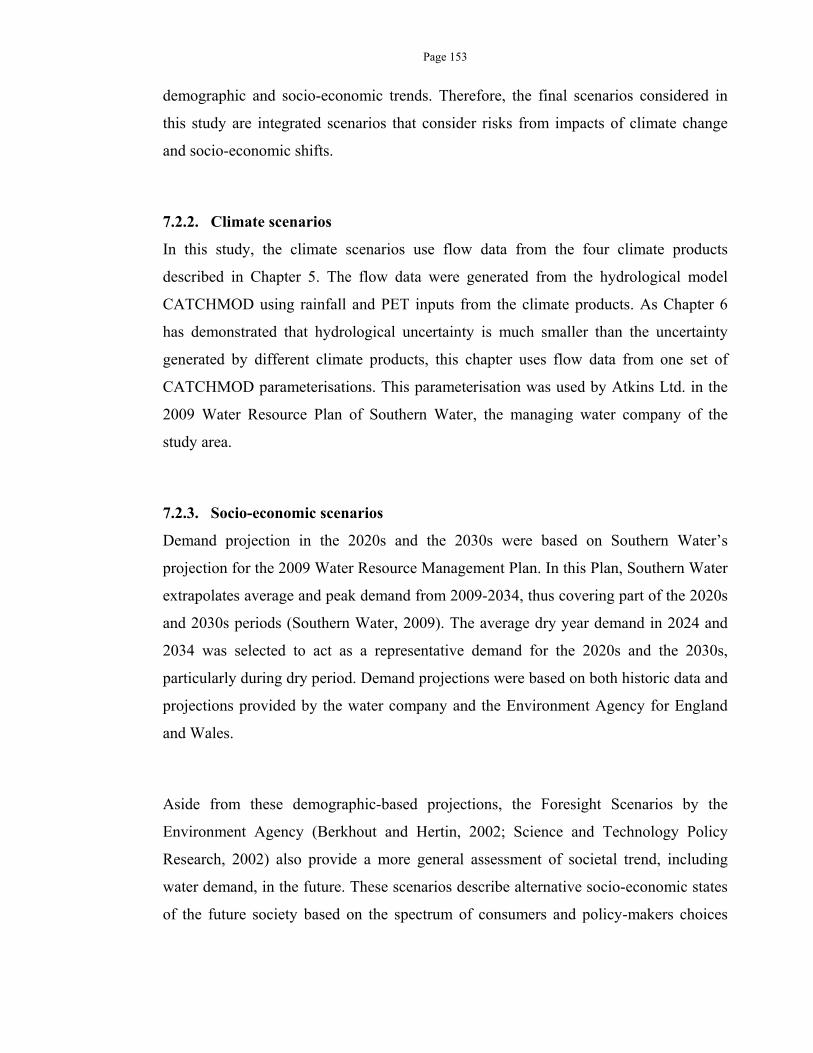
Page 153
demographic and socio-economic trends. Therefore, the final scenarios considered in
this study are integrated scenarios that consider risks from impacts of climate change
and socio-economic shifts.
7.2.2. Climate scenarios
In this study, the climate scenarios use flow data from the four climate products
described in Chapter 5. The flow data were generated from the hydrological model
CATCHMOD using rainfall and PET inputs from the climate products. As Chapter 6
has demonstrated that hydrological uncertainty is much smaller than the uncertainty
generated by different climate products, this chapter uses flow data from one set of
CATCHMOD parameterisations. This parameterisation was used by Atkins Ltd. in the
2009 Water Resource Plan of Southern Water, the managing water company of the
study area.
7.2.3. Socio-economic scenarios
Demand projection in the 2020s and the 2030s were based on Southern Water’s
projection for the 2009 Water Resource Management Plan. In this Plan, Southern Water
extrapolates average and peak demand from 2009-2034, thus covering part of the 2020s
and 2030s periods (Southern Water, 2009). The average dry year demand in 2024 and
2034 was selected to act as a representative demand for the 2020s and the 2030s,
particularly during dry period. Demand projections were based on both historic data and
projections provided by the water company and the Environment Agency for England
and Wales.
Aside from these demographic-based projections, the Foresight Scenarios by the
Environment Agency (Berkhout and Hertin, 2002; Science and Technology Policy
Research, 2002) also provide a more general assessment of societal trend, including
water demand, in the future. These scenarios describe alternative socio-economic states
of the future society based on the spectrum of consumers and policy-makers choices
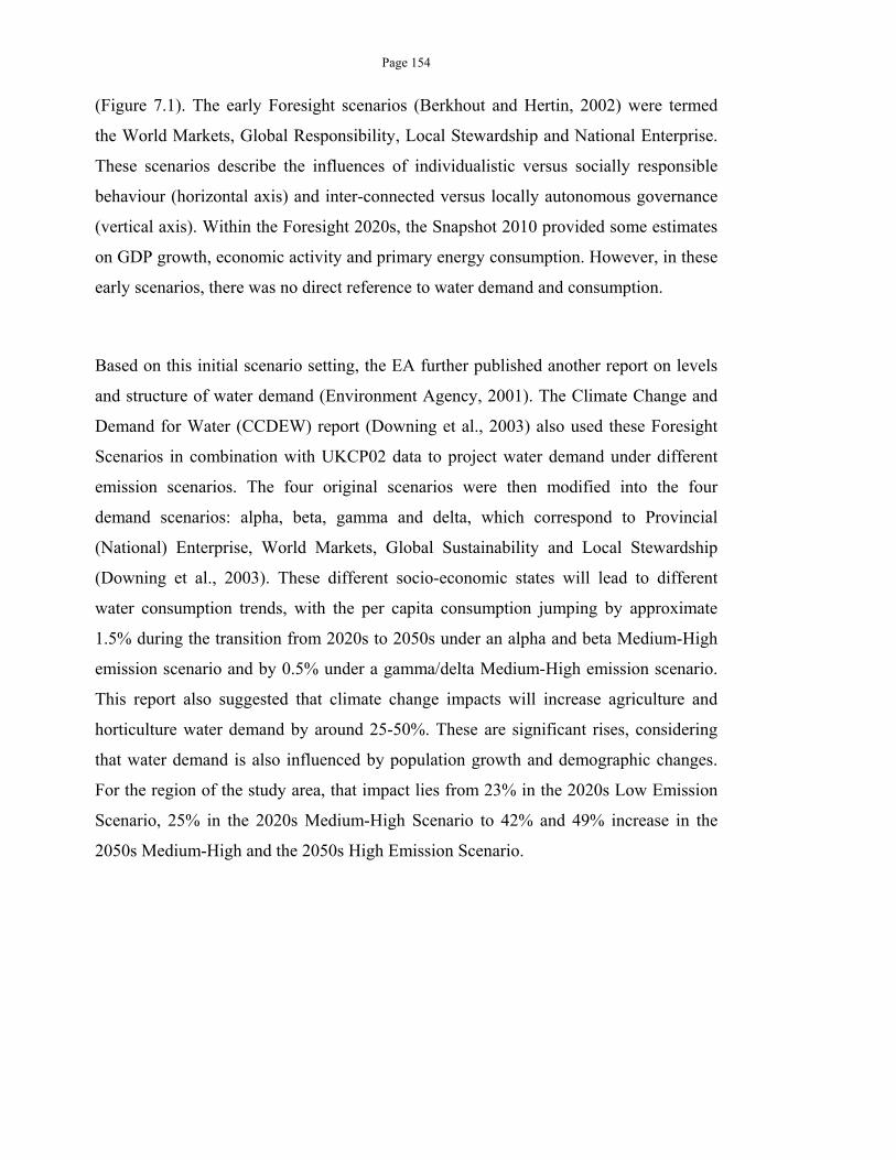
Page 154
(Figure 7.1). The early Foresight scenarios (Berkhout and Hertin, 2002) were termed
the World Markets, Global Responsibility, Local Stewardship and National Enterprise.
These scenarios describe the influences of individualistic versus socially responsible
behaviour (horizontal axis) and inter-connected versus locally autonomous governance
(vertical axis). Within the Foresight 2020s, the Snapshot 2010 provided some estimates
on GDP growth, economic activity and primary energy consumption. However, in these
early scenarios, there was no direct reference to water demand and consumption.
Based on this initial scenario setting, the EA further published another report on levels
and structure of water demand (Environment Agency, 2001). The Climate Change and
Demand for Water (CCDEW) report (Downing et al., 2003) also used these Foresight
Scenarios in combination with UKCP02 data to project water demand under different
emission scenarios. The four original scenarios were then modified into the four
demand scenarios: alpha, beta, gamma and delta, which correspond to Provincial
(National) Enterprise, World Markets, Global Sustainability and Local Stewardship
(Downing et al., 2003). These different socio-economic states will lead to different
water consumption trends, with the per capita consumption jumping by approximate
1.5% during the transition from 2020s to 2050s under an alpha and beta Medium-High
emission scenario and by 0.5% under a gamma/delta Medium-High emission scenario.
This report also suggested that climate change impacts will increase agriculture and
horticulture water demand by around 25-50%. These are significant rises, considering
that water demand is also influenced by population growth and demographic changes.
For the region of the study area, that impact lies from 23% in the 2020s Low Emission
Scenario, 25% in the 2020s Medium-High Scenario to 42% and 49% increase in the
2050s Medium-High and the 2050s High Emission Scenario.
Page 155
Figure 7.1 Four UK Future Scenarios for 2020s. Source: Science and Technology Policy Research (2002)
These storylines were further revisited and modified in the EA Scenarios for the 2030s
and the 2050s. While the consumer attitude spectrum was slightly modified to reflect
more closely the varying degrees of sustainability awareness, the governance axis was
phrased explicitly into sustainability versus short-term socio-economic concerns instead
of local versus globalised governance such as in the previous version. These scenarios,
however, did not come with any assessment on water demand trends, all four scenarios
share the same assumption of average per-capita water consumption of 153 l/d/capita
and the different water consumption patterns in each scenario were described
qualitatively. Figure 7.2 presents this version of the four 2030s Future Scenarios in a
similar position to the 2020s scenarios. The 2030s scenarios appear to partially correlate
to the SRES and the Foresight set (Burdett et al., 2006), in particular A1.-
Jeopardy/Alchemy-World Markets; A2-Local Stewardship-Survivor; B1-
Restoration/Alchemy-Global Sustainability; and B2-Local Stewardship-
Survivor/Alchemy.
Page 156
Figure 7.2 The 2030s four EA scenarios. Source: Burdett et al. (2006)
Finally, the newer Environment Agency projects demonstrate demand shifts for the
2050s under four scenarios, termed Sustainable Behaviour, Innovation, Local Resilience
and Market Forces. Each of these scenarios reflects a different mode of governance and
consumption (Environment Agency, 2008) (Figure 7.3). In essence, the projected
change is as follows:
Innovation (I): Total Demand reduces by 4%, water per capita consumption
(pcc) 125 l/d/capita. The responsibility to find adaptation strategies lies with the
government and scientist; demand reduction is due to sustainability-led
governance and technological innovation.
Market Forces (MF): Total Demand increases by 35%, pcc 165 l/d/capita.
Water demand is driven by the market trend, focusing on cost optimisation and
growth.
Local Resilience (LR): Total Demand increases by 8%; pcc is 140 l/d/capita.
People realise the need for demand reduction and take actions towards it. Their
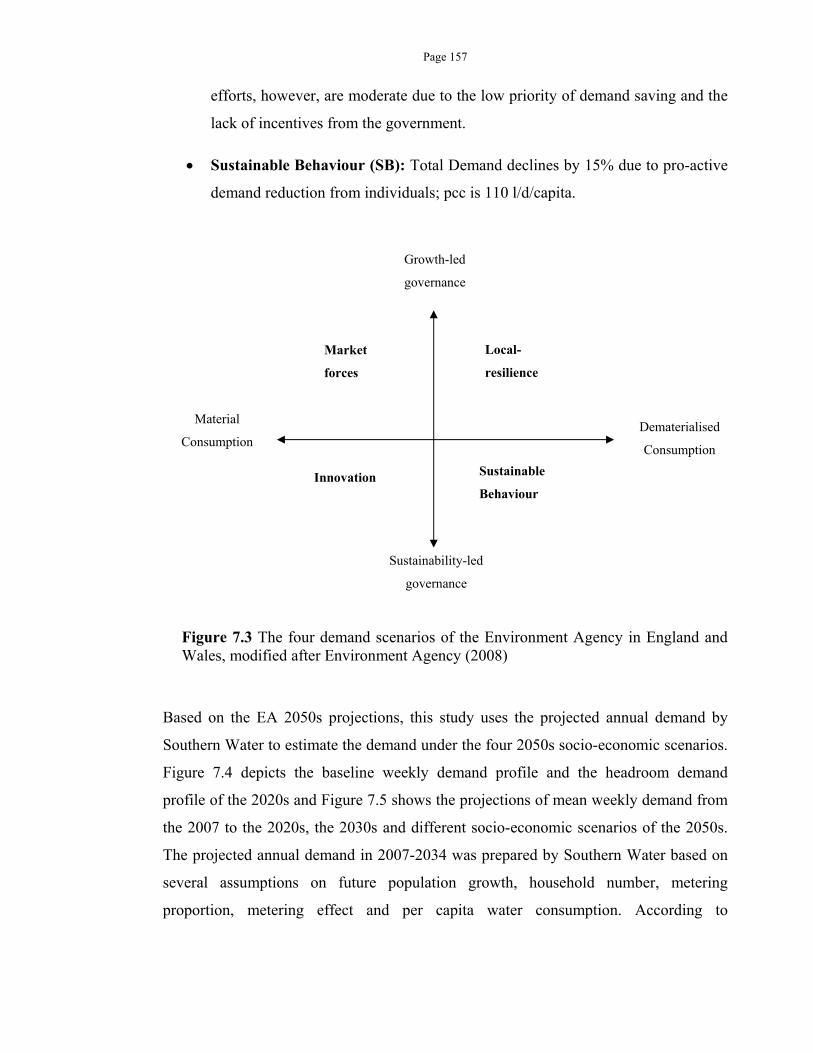
Page 157
efforts, however, are moderate due to the low priority of demand saving and the
lack of incentives from the government.
Sustainable Behaviour (SB): Total Demand declines by 15% due to pro-active
demand reduction from individuals; pcc is 110 l/d/capita.
Figure 7.3 The four demand scenarios of the Environment Agency in England and Wales, modified after Environment Agency (2008)
Based on the EA 2050s projections, this study uses the projected annual demand by
Southern Water to estimate the demand under the four 2050s socio-economic scenarios.
Figure 7.4 depicts the baseline weekly demand profile and the headroom demand
profile of the 2020s and Figure 7.5 shows the projections of mean weekly demand from
the 2007 to the 2020s, the 2030s and different socio-economic scenarios of the 2050s.
The projected annual demand in 2007-2034 was prepared by Southern Water based on
several assumptions on future population growth, household number, metering
proportion, metering effect and per capita water consumption. According to
Dematerialised
Consumption
Sustainable
Behaviour Innovation
Local-
resilience
Market
forces
Growth-led
governance
Material
Consumption
Sustainability-led
governance
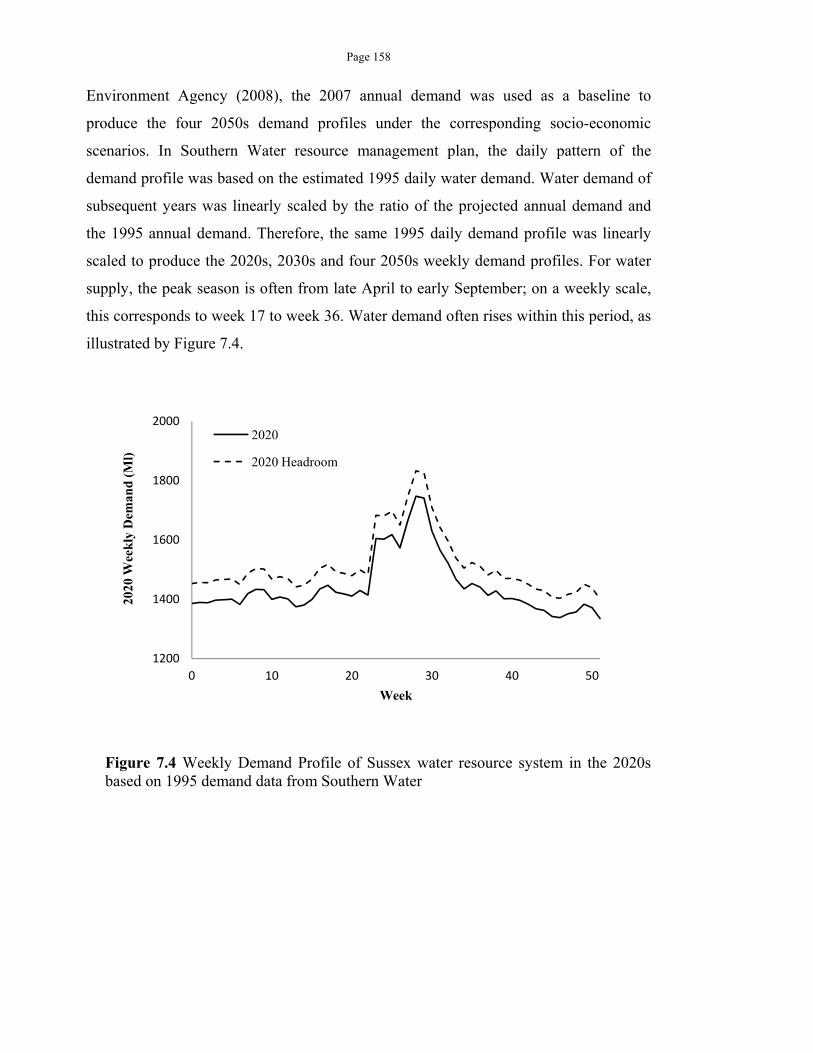
Page 158
Environment Agency (2008), the 2007 annual demand was used as a baseline to
produce the four 2050s demand profiles under the corresponding socio-economic
scenarios. In Southern Water resource management plan, the daily pattern of the
demand profile was based on the estimated 1995 daily water demand. Water demand of
subsequent years was linearly scaled by the ratio of the projected annual demand and
the 1995 annual demand. Therefore, the same 1995 daily demand profile was linearly
scaled to produce the 2020s, 2030s and four 2050s weekly demand profiles. For water
supply, the peak season is often from late April to early September; on a weekly scale,
this corresponds to week 17 to week 36. Water demand often rises within this period, as
illustrated by Figure 7.4.
Figure 7.4 Weekly Demand Profile of Sussex water resource system in the 2020s based on 1995 demand data from Southern Water
1200
1400
1600
1800
2000
0 10 20 30 40 50
2020
Wee
kly
Dem
and
(M
l)
Week
2020
2020 Headroom
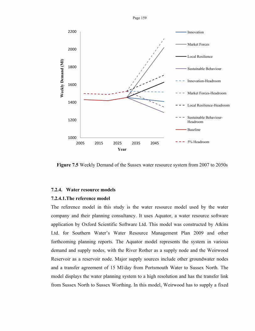
Page 159
Figure 7.5 Weekly Demand of the Sussex water resource system from 2007 to 2050s
7.2.4. Water resource models
7.2.4.1.The reference model
The reference model in this study is the water resource model used by the water
company and their planning consultancy. It uses Aquator, a water resource software
application by Oxford Scientific Software Ltd. This model was constructed by Atkins
Ltd. for Southern Water’s Water Resource Management Plan 2009 and other
forthcoming planning reports. The Aquator model represents the system in various
demand and supply nodes, with the River Rother as a supply node and the Weirwood
Reservoir as a reservoir node. Major supply sources include other groundwater nodes
and a transfer agreement of 15 Ml/day from Portsmouth Water to Sussex North. The
model displays the water planning system to a high resolution and has the transfer link
from Sussex North to Sussex Worthing. In this model, Weirwood has to supply a fixed
1000
1200
1400
1600
1800
2000
2200
2005 2015 2025 2035 2045
Wee
kly
Dem
and
(M
l)
Year
Innovation
Market Forces
Local Resilience
Sustainable Behaviour
Innovation-Headroom
Market Forces-Headroom
Local Resilience-Headroom
Sustainable Behaviour-Headroom
Baseline
5% Headroom
Page 160
amount to South East Water before it can input water into other sources. Network
analysis also shows that Weirwood can only input water into two nodes, the rest of the
region being supplied by other sources. The demand profile used in the Aquator model
was constructed by Atkins based on the same 1995 regional demand profile; water
demand at individual nodes can vary slightly but overall sum up to the total regional
demand profile on a daily scale. For a schematic of the model, please refer to Appendix
A.
7.2.4.2.The VB.NET Simulation Model
This model was coded in VB.NET based on an Excel-based model by Wade (2005).
Model parameters include the supply and demand capacity/profile of each node, the
transfer capacity of each link, reservoir storage, reservoir operational curve and
reservoir pumping capacity. The model consists of the River Rother, Weirwood,
Hardham groundwater, other groundwater sources and transfer to and from other water
companies (South East Water and Portsmouth Water). The model can use time series
for groundwater sources and demand profile. All the demand nodes in each water
resource zone were congregated into one to two regional demand nodes (Figure 7.6).
These regional demands were constructed by summing the relevant individual demand
profiles of the AQUATOR. Like the AQUATOR model, the groundwater nodes are
subject to daily and annual licenses. This model simplifies the AQUATOR model to the
scale of water resource zones, with each zone consisting of major proxy nodes instead
of individual AQUATOR nodes. In particular, the Sussex North supply still includes the
supply nods of Portsmouth, Hardham Groundwater, River Rother and Weirwood
Reservoir. The link constraint representing the treatment capacity of the Hardham
Water Supply Work (WSW) is included in the model; other transfer constrains within
smaller demand nodes, however, does not present since these nodes have been
aggregated into a single node. The supply from the Weirwood Reservoir is restricted by
its pumping capacity of 21.8 Ml/day. Overall the demand for the Sussex North area is
represented by the Sussex Demand node, the transfer agreement from Weirwood
Reservoir is represented by the South East Water Transfer node. Similarly, the
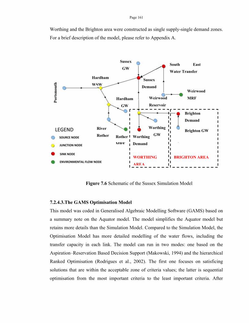
Page 161
Worthing and the Brighton area were constructed as single supply-single demand zones.
For a brief description of the model, please refer to Appendix A.
Figure 7.6 Schematic of the Sussex Simulation Model
7.2.4.3.The GAMS Optimisation Model
This model was coded in Generalised Algebraic Modelling Software (GAMS) based on
a summary note on the Aquator model. The model simplifies the Aquator model but
retains more details than the Simulation Model. Compared to the Simulation Model, the
Optimisation Model has more detailed modelling of the water flows, including the
transfer capacity in each link. The model can run in two modes: one based on the
Aspiration–Reservation Based Decision Support (Makowski, 1994) and the hierarchical
Ranked Optimisation (Rodrigues et al., 2002). The first one focuses on satisficing
solutions that are within the acceptable zone of criteria values; the latter is sequential
optimisation from the most important criteria to the least important criteria. After
Por
tsm
outh
Sussex
GWSouth East
Water Transfer
Weirwood
MRF Weirwood
Reservoir
River
Rother Rother
MRF
Hardham
GW
Hardham
WSW
Worthing
GW Worthing
Demand
WORTHING
AREA
Brighton
Demand
Brighton GW
BRIGHTON AREA
Sussex
Demand
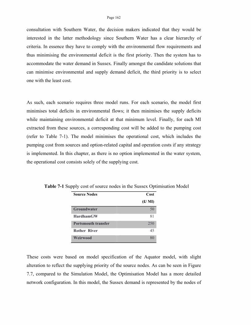
Page 162
consultation with Southern Water, the decision makers indicated that they would be
interested in the latter methodology since Southern Water has a clear hierarchy of
criteria. In essence they have to comply with the environmental flow requirements and
thus minimising the environmental deficit is the first priority. Then the system has to
accommodate the water demand in Sussex. Finally amongst the candidate solutions that
can minimise environmental and supply demand deficit, the third priority is to select
one with the least cost.
As such, each scenario requires three model runs. For each scenario, the model first
minimises total deficits in environmental flows; it then minimises the supply deficits
while maintaining environmental deficit at that minimum level. Finally, for each Ml
extracted from these sources, a corresponding cost will be added to the pumping cost
(refer to Table 7-1). The model minimises the operational cost, which includes the
pumping cost from sources and option-related capital and operation costs if any strategy
is implemented. In this chapter, as there is no option implemented in the water system,
the operational cost consists solely of the supplying cost.
Table 7-1 Supply cost of source nodes in the Sussex Optimisation Model
Source Nodes Cost
(£/ Ml)
Groundwater 50
HardhamGW 81
Portsmouth transfer 250
Rother River 45
Weirwood 80
These costs were based on model specification of the Aquator model, with slight
alteration to reflect the supplying priority of the source nodes. As can be seen in Figure
7.7, compared to the Simulation Model, the Optimisation Model has a more detailed
network configuration. In this model, the Sussex demand is represented by the nodes of
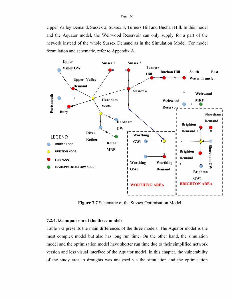
Page 163
Upper Valley Demand, Sussex 2, Sussex 3, Turners Hill and Buchan Hill. In this model
and the Aquator model, the Weirwood Reservoir can only supply for a part of the
network instead of the whole Sussex Demand as in the Simulation Model. For model
formulation and schematic, refer to Appendix A.
Figure 7.7 Schematic of the Sussex Optimisation Model
7.2.4.4.Comparison of the three models
Table 7-2 presents the main differences of the three models. The Aquator model is the
most complex model but also has long run time. On the other hand, the simulation
model and the optimisation model have shorter run time due to their simplified network
version and less visual interface of the Aquator model. In this chapter, the vulnerability
of the study area to droughts was analysed via the simulation and the optimisation
Weirwood
Reservoir
Brighton
Demand
2
Hardham
WSW
Bury
Brighton
Demand 1
Hardham
GWRiver
Rother
Por
tsm
outh
Sussex 4
Upper Valley
Demand
Worthing
GW2
Worthing
Demand
Sh
oreham
GW
Brighton
GW1
Weirwood
MRF
Shoreham
Demand
South East
Water Transfer
Buchan Hill Turners
Hill
Sussex 3 Sussex 2 Upper
Valley GW
BRIGHTON AREA
WORTHING AREA
Worthing
GW1 Rother
MRF
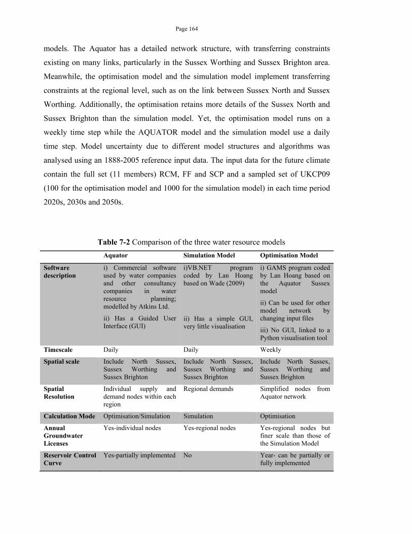
Page 164
models. The Aquator has a detailed network structure, with transferring constraints
existing on many links, particularly in the Sussex Worthing and Sussex Brighton area.
Meanwhile, the optimisation model and the simulation model implement transferring
constraints at the regional level, such as on the link between Sussex North and Sussex
Worthing. Additionally, the optimisation retains more details of the Sussex North and
Sussex Brighton than the simulation model. Yet, the optimisation model runs on a
weekly time step while the AQUATOR model and the simulation model use a daily
time step. Model uncertainty due to different model structures and algorithms was
analysed using an 1888-2005 reference input data. The input data for the future climate
contain the full set (11 members) RCM, FF and SCP and a sampled set of UKCP09
(100 for the optimisation model and 1000 for the simulation model) in each time period
2020s, 2030s and 2050s.
Table 7-2 Comparison of the three water resource models
Aquator Simulation Model Optimisation Model
Software description
i) Commercial software used by water companies and other consultancy companies in water resource planning; modelled by Atkins Ltd.
ii) Has a Guided User Interface (GUI)
i)VB.NET program coded by Lan Hoang based on Wade (2009)
ii) Has a simple GUI, very little visualisation
i) GAMS program coded by Lan Hoang based on the Aquator Sussex model
ii) Can be used for other model network by changing input files
iii) No GUI, linked to a Python visualisation tool
Timescale Daily Daily Weekly
Spatial scale Include North Sussex, Sussex Worthing and Sussex Brighton
Include North Sussex, Sussex Worthing and Sussex Brighton
Include North Sussex, Sussex Worthing and Sussex Brighton
Spatial Resolution
Individual supply and demand nodes within each region
Regional demands Simplified nodes from Aquator network
Calculation Mode Optimisation/Simulation Simulation Optimisation
Annual Groundwater Licenses
Yes-individual nodes Yes-regional nodes Yes-regional nodes but finer scale than those of the Simulation Model
Reservoir Control Curve
Yes-partially implemented No Year- can be partially or fully implemented
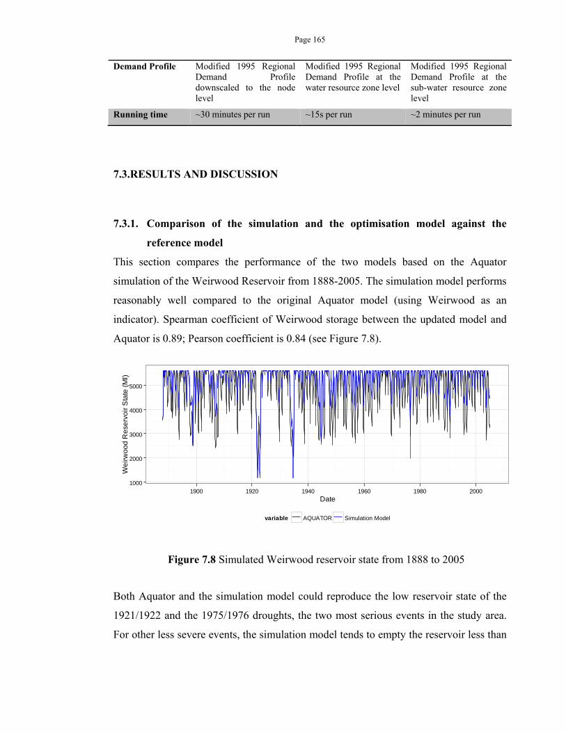
Page 165
Demand Profile Modified 1995 Regional Demand Profile downscaled to the node level
Modified 1995 Regional Demand Profile at the water resource zone level
Modified 1995 Regional Demand Profile at the sub-water resource zone level
Running time ~30 minutes per run ~15s per run ~2 minutes per run
7.3.RESULTS AND DISCUSSION
7.3.1. Comparison of the simulation and the optimisation model against the
reference model
This section compares the performance of the two models based on the Aquator
simulation of the Weirwood Reservoir from 1888-2005. The simulation model performs
reasonably well compared to the original Aquator model (using Weirwood as an
indicator). Spearman coefficient of Weirwood storage between the updated model and
Aquator is 0.89; Pearson coefficient is 0.84 (see Figure 7.8).
Figure 7.8 Simulated Weirwood reservoir state from 1888 to 2005
Both Aquator and the simulation model could reproduce the low reservoir state of the
1921/1922 and the 1975/1976 droughts, the two most serious events in the study area.
For other less severe events, the simulation model tends to empty the reservoir less than
1000
2000
3000
4000
5000
1900 1920 1940 1960 1980 2000Date
We
irw
oo
d R
ese
rvo
ir S
tate
(M
l)
variable AQUATOR Simulation Model
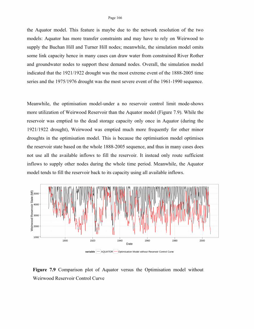
Page 166
the Aquator model. This feature is maybe due to the network resolution of the two
models: Aquator has more transfer constraints and may have to rely on Weirwood to
supply the Buchan Hill and Turner Hill nodes; meanwhile, the simulation model omits
some link capacity hence in many cases can draw water from constrained River Rother
and groundwater nodes to support these demand nodes. Overall, the simulation model
indicated that the 1921/1922 drought was the most extreme event of the 1888-2005 time
series and the 1975/1976 drought was the most severe event of the 1961-1990 sequence.
Meanwhile, the optimisation model-under a no reservoir control limit mode-shows
more utilization of Weirwood Reservoir than the Aquator model (Figure 7.9). While the
reservoir was emptied to the dead storage capacity only once in Aquator (during the
1921/1922 drought), Weirwood was emptied much more frequently for other minor
droughts in the optimisation model. This is because the optimisation model optimises
the reservoir state based on the whole 1888-2005 sequence, and thus in many cases does
not use all the available inflows to fill the reservoir. It instead only route sufficient
inflows to supply other nodes during the whole time period. Meanwhile, the Aquator
model tends to fill the reservoir back to its capacity using all available inflows.
Figure 7.9 Comparison plot of Aquator versus the Optimisation model without
Weirwood Reservoir Control Curve
1000
2000
3000
4000
5000
1900 1920 1940 1960 1980 2000Date
We
irw
oo
d R
ese
rvo
ir S
tate
(M
l)
variable AQUATOR Optimisation Model without Reservoir Control Curve
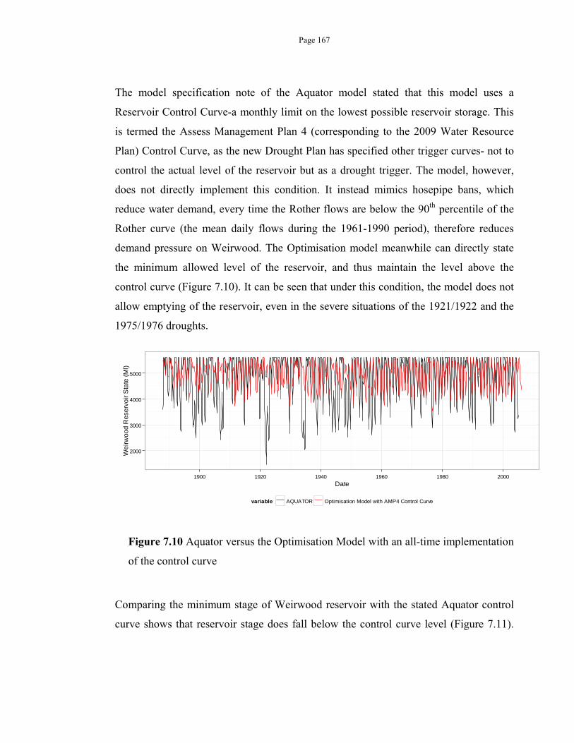
Page 167
The model specification note of the Aquator model stated that this model uses a
Reservoir Control Curve-a monthly limit on the lowest possible reservoir storage. This
is termed the Assess Management Plan 4 (corresponding to the 2009 Water Resource
Plan) Control Curve, as the new Drought Plan has specified other trigger curves- not to
control the actual level of the reservoir but as a drought trigger. The model, however,
does not directly implement this condition. It instead mimics hosepipe bans, which
reduce water demand, every time the Rother flows are below the 90th percentile of the
Rother curve (the mean daily flows during the 1961-1990 period), therefore reduces
demand pressure on Weirwood. The Optimisation model meanwhile can directly state
the minimum allowed level of the reservoir, and thus maintain the level above the
control curve (Figure 7.10). It can be seen that under this condition, the model does not
allow emptying of the reservoir, even in the severe situations of the 1921/1922 and the
1975/1976 droughts.
Figure 7.10 Aquator versus the Optimisation Model with an all-time implementation
of the control curve
Comparing the minimum stage of Weirwood reservoir with the stated Aquator control
curve shows that reservoir stage does fall below the control curve level (Figure 7.11).
2000
3000
4000
5000
1900 1920 1940 1960 1980 2000Date
Wei
rwo
od
Re
serv
oir
Sta
te (
Ml)
variable AQUATOR Optimisation Model with AMP4 Control Curve
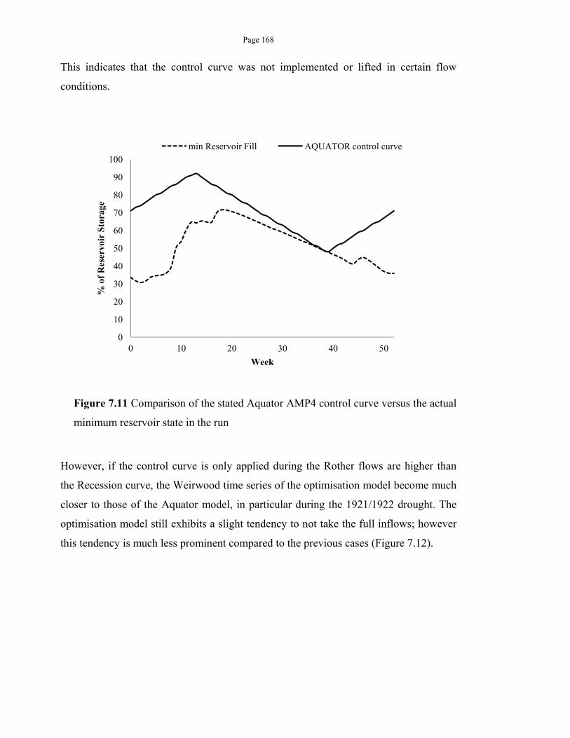
Page 168
This indicates that the control curve was not implemented or lifted in certain flow
conditions.
Figure 7.11 Comparison of the stated Aquator AMP4 control curve versus the actual
minimum reservoir state in the run
However, if the control curve is only applied during the Rother flows are higher than
the Recession curve, the Weirwood time series of the optimisation model become much
closer to those of the Aquator model, in particular during the 1921/1922 drought. The
optimisation model still exhibits a slight tendency to not take the full inflows; however
this tendency is much less prominent compared to the previous cases (Figure 7.12).
0
10
20
30
40
50
60
70
80
90
100
0 10 20 30 40 50
% o
f R
eser
voir
Sto
rage
Week
min Reservoir Fill AQUATOR control curve
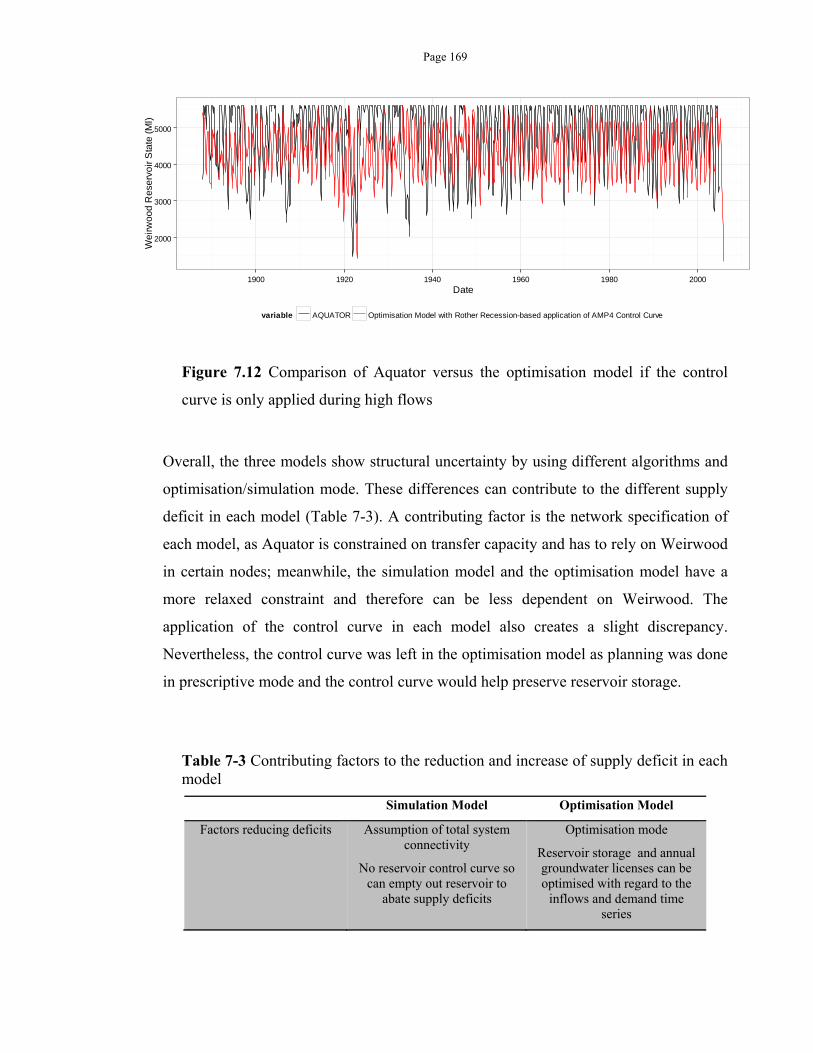
Page 169
Figure 7.12 Comparison of Aquator versus the optimisation model if the control
curve is only applied during high flows
Overall, the three models show structural uncertainty by using different algorithms and
optimisation/simulation mode. These differences can contribute to the different supply
deficit in each model (Table 7-3). A contributing factor is the network specification of
each model, as Aquator is constrained on transfer capacity and has to rely on Weirwood
in certain nodes; meanwhile, the simulation model and the optimisation model have a
more relaxed constraint and therefore can be less dependent on Weirwood. The
application of the control curve in each model also creates a slight discrepancy.
Nevertheless, the control curve was left in the optimisation model as planning was done
in prescriptive mode and the control curve would help preserve reservoir storage.
Table 7-3 Contributing factors to the reduction and increase of supply deficit in each model
Simulation Model Optimisation Model
Factors reducing deficits Assumption of total system connectivity
No reservoir control curve so can empty out reservoir to
abate supply deficits
Optimisation mode
Reservoir storage and annual groundwater licenses can be optimised with regard to the
inflows and demand time series
2000
3000
4000
5000
1900 1920 1940 1960 1980 2000Date
We
irw
oo
d R
ese
rvo
ir S
tate
(M
l)
variable AQUATOR Optimisation Model with Rother Recession-based application of AMP4 Control Curve
Page 170
Coarse time step
Factors increasing deficits Simulation mode
Daily time step-can be subject to severe shortage at a daily
time scale
Constraints on link capacity
Reservoir control curve can prevent water release
The optimisation and the simulation model were then used to further analyse the
vulnerability under changing climate and water demand, according to the four climate
products. The Aquator model was not used due to its time and computational
requirements. Results from the optimisation and the simulation model were then
compared to indicate any possible structure uncertainty and the range of climate and
demand risks to the study area.
7.3.2. Simulation model results
The simulation model confirms that the water system is sensitive to drought conditions
of the 1975-1976 and 1921-1922. If tested against the whole time series from 1888-
2005, the drought period that brought the worst supply deficit were the 1921-1922
period. Otherwise, for a shortened time series of 1961 onwards, the 1975-1976 was the
most serious drought. Model results using the four climate products again confirm the
high level of uncertainty on possible impacts (Figure 7.13). In essence, the RCM and FF
time series pose a higher risk of supply deficit than the SCP and the UKCP09 groups.
While being significantly drier than the FF group in terms of rainfall (refer to Chapter
5), the RCM time series create a similar risk level to FF. The UKCP09 product, due to
its wide range Bayesian probabilistic scenarios, projects a wide range of possible deficit
prospects but not to the risk level of the FF and the RCM groups.
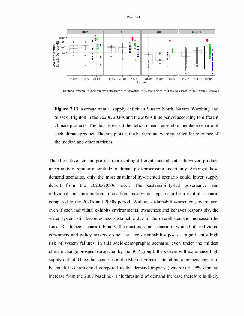
Page 171
Figure 7.13 Average annual supply deficit in Sussex North, Sussex Worthing and
Sussex Brighton in the 2020s, 2030s and the 2050s time period according to different
climate products. The dots represent the deficit in each ensemble member/scenario of
each climate product. The box plots at the background were provided for reference of
the median and other statistics.
The alternative demand profiles representing different societal states, however, produce
uncertainty of similar magnitude to climate post-processing uncertainty. Amongst these
demand scenarios, only the most sustainability-oriented scenario could lower supply
deficit from the 2020s/2030s level. The sustainability-led governance and
individualistic consumption, Innovation, meanwhile appears to be a neutral scenario
compared to the 2020s and 2030s period. Without sustainability-oriented governance,
even if each individual exhibits environmental awareness and behaves responsibly, the
water system still becomes less sustainable due to the overall demand increases (the
Local Resilience scenario). Finally, the most extreme scenario in which both individual
consumers and policy makers do not care for sustainability poses a significantly high
risk of system failures. In this socio-demographic scenario, even under the mildest
climate change prospect (projected by the SCP group), the system will experience high
supply deficit. Once the society is at the Market Forces state, climate impacts appear to
be much less influential compared to the demand impacts (which is a 35% demand
increase from the 2007 baseline). This threshold of demand increase therefore is likely
RCM FF SCP UKCP09
10
100
1000
5000
2020s 2030s 2050s 2020s 2030s 2050s 2020s 2030s 2050s 2020s 2030s 2050sPeriod
Ave
rag
e A
nn
ua
l S
up
ply
De
ficit
(Ml)
Demand Profiles Southern Water Basecase Innovation Market Forces Local Resilience Sustainable Behaviour
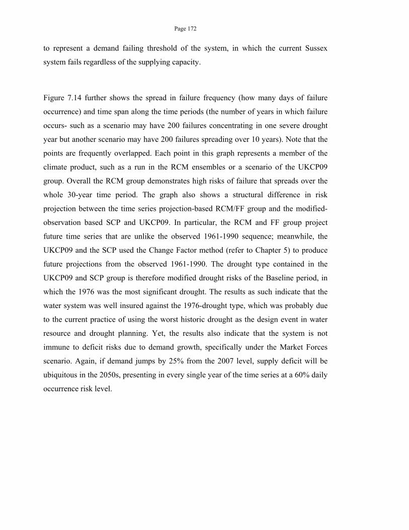
Page 172
to represent a demand failing threshold of the system, in which the current Sussex
system fails regardless of the supplying capacity.
Figure 7.14 further shows the spread in failure frequency (how many days of failure
occurrence) and time span along the time periods (the number of years in which failure
occurs- such as a scenario may have 200 failures concentrating in one severe drought
year but another scenario may have 200 failures spreading over 10 years). Note that the
points are frequently overlapped. Each point in this graph represents a member of the
climate product, such as a run in the RCM ensembles or a scenario of the UKCP09
group. Overall the RCM group demonstrates high risks of failure that spreads over the
whole 30-year time period. The graph also shows a structural difference in risk
projection between the time series projection-based RCM/FF group and the modified-
observation based SCP and UKCP09. In particular, the RCM and FF group project
future time series that are unlike the observed 1961-1990 sequence; meanwhile, the
UKCP09 and the SCP used the Change Factor method (refer to Chapter 5) to produce
future projections from the observed 1961-1990. The drought type contained in the
UKCP09 and SCP group is therefore modified drought risks of the Baseline period, in
which the 1976 was the most significant drought. The results as such indicate that the
water system was well insured against the 1976-drought type, which was probably due
to the current practice of using the worst historic drought as the design event in water
resource and drought planning. Yet, the results also indicate that the system is not
immune to deficit risks due to demand growth, specifically under the Market Forces
scenario. Again, if demand jumps by 25% from the 2007 level, supply deficit will be
ubiquitous in the 2050s, presenting in every single year of the time series at a 60% daily
occurrence risk level.
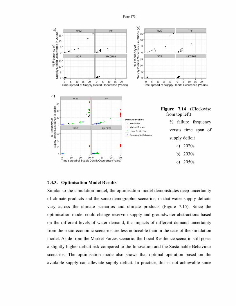
Page 173
Figure 7.14 (Clockwise from top left)
% failure frequency
versus time span of
supply deficit
a) 2020s
b) 2030s
c) 2050s
7.3.3. Optimisation Model Results
Similar to the simulation model, the optimisation model demonstrates deep uncertainty
of climate products and the socio-demographic scenarios, in that water supply deficits
vary across the climate scenarios and climate products (Figure 7.15). Since the
optimisation model could change reservoir supply and groundwater abstractions based
on the different levels of water demand, the impacts of different demand uncertainty
from the socio-economic scenarios are less noticeable than in the case of the simulation
model. Aside from the Market Forces scenario, the Local Resilience scenario still poses
a slightly higher deficit risk compared to the Innovation and the Sustainable Behaviour
scenarios. The optimisation mode also shows that optimal operation based on the
available supply can alleviate supply deficit. In practice, this is not achievable since
RCM FF
SCP UKCP09
0
5
10
15
0
5
10
15
0 5 10 15 20 0 5 10 15 20Time spread of Supply Decifit Occurence (Years)
% F
requ
ency
of
Supply
Defic
it O
ccurr
ence
in 2
020
s RCM FF
SCP UKCP09
0
5
10
15
0
5
10
15
0 5 10 15 20 0 5 10 15 20Time spread of Supply Decifit Occurence (Years)
% F
req
ue
ncy
of
Su
pp
ly D
efic
it O
ccu
rre
nce
in 2
03
0s
RCM FF
SCP UKCP09
0
20
40
60
0
20
40
60
0 10 20 30 0 10 20 30Time spread of Supply Decifit Occurence (Years)
% F
requ
enc
y of
S
upply
Defic
it O
ccurr
enc
e in
205
0s
Demand Profiles
Innovation
Market Forces
Local Resilience
Sustainable Behaviour
a) b)
c)
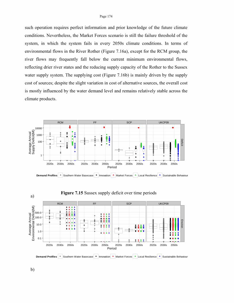
Page 174
such operation requires perfect information and prior knowledge of the future climate
conditions. Nevertheless, the Market Forces scenario is still the failure threshold of the
system, in which the system fails in every 2050s climate conditions. In terms of
environmental flows in the River Rother (Figure 7.16a), except for the RCM group, the
river flows may frequently fall below the current minimum environmental flows,
reflecting drier river states and the reducing supply capacity of the Rother to the Sussex
water supply system. The supplying cost (Figure 7.16b) is mainly driven by the supply
cost of sources; despite the slight variation in cost of alternative sources, the overall cost
is mostly influenced by the water demand level and remains relatively stable across the
climate products.
Figure 7.15 Sussex supply deficit over time periods
RCM FF SCP UKCP09
1
100
1000
10000
Deficit
2020s 2030s 2050s 2020s 2030s 2050s 2020s 2030s 2050s 2020s 2030s 2050sPeriod
Ave
rag
e A
nn
ua
l S
up
ply
De
ficit(
Ml)
Demand Profiles Southern Water Basecase Innovation Market Forces Local Resilience Sustainable Behaviour
RCM FF SCP UKCP09
0.1
1.0
10.0
100.0
500.0
Environ
2020s 2030s 2050s 2020s 2030s 2050s 2020s 2030s 2050s 2020s 2030s 2050sPeriod
Ave
rag
e A
nn
ua
l E
nvi
ron
me
nta
l De
ficit(
Ml)
Demand Profiles Southern Water Basecase Innovation Market Forces Local Resilience Sustainable Behaviour
a)
b)
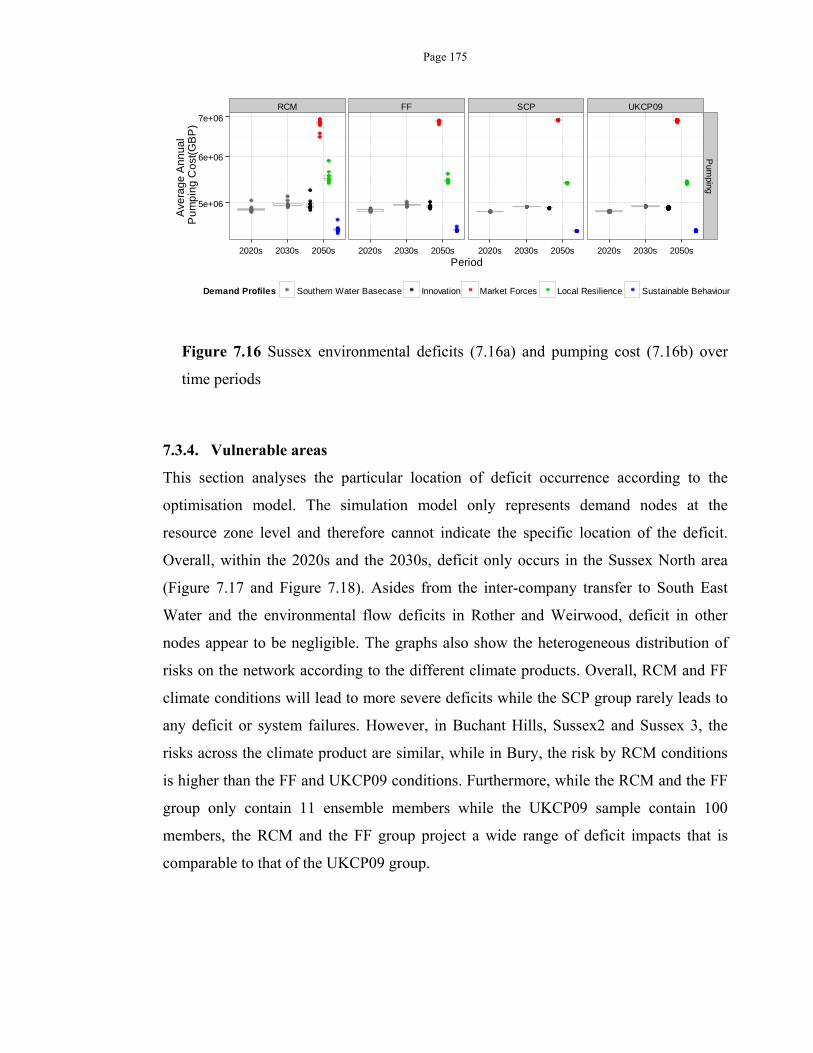
Page 175
Figure 7.16 Sussex environmental deficits (7.16a) and pumping cost (7.16b) over
time periods
7.3.4. Vulnerable areas
This section analyses the particular location of deficit occurrence according to the
optimisation model. The simulation model only represents demand nodes at the
resource zone level and therefore cannot indicate the specific location of the deficit.
Overall, within the 2020s and the 2030s, deficit only occurs in the Sussex North area
(Figure 7.17 and Figure 7.18). Asides from the inter-company transfer to South East
Water and the environmental flow deficits in Rother and Weirwood, deficit in other
nodes appear to be negligible. The graphs also show the heterogeneous distribution of
risks on the network according to the different climate products. Overall, RCM and FF
climate conditions will lead to more severe deficits while the SCP group rarely leads to
any deficit or system failures. However, in Buchant Hills, Sussex2 and Sussex 3, the
risks across the climate product are similar, while in Bury, the risk by RCM conditions
is higher than the FF and UKCP09 conditions. Furthermore, while the RCM and the FF
group only contain 11 ensemble members while the UKCP09 sample contain 100
members, the RCM and the FF group project a wide range of deficit impacts that is
comparable to that of the UKCP09 group.
RCM FF SCP UKCP09
5e+06
6e+06
7e+06
Pum
ping
2020s 2030s 2050s 2020s 2030s 2050s 2020s 2030s 2050s 2020s 2030s 2050sPeriod
Ave
rag
e A
nn
ua
l P
um
pin
g C
ost
(GB
P)
Demand Profiles Southern Water Basecase Innovation Market Forces Local Resilience Sustainable Behaviour
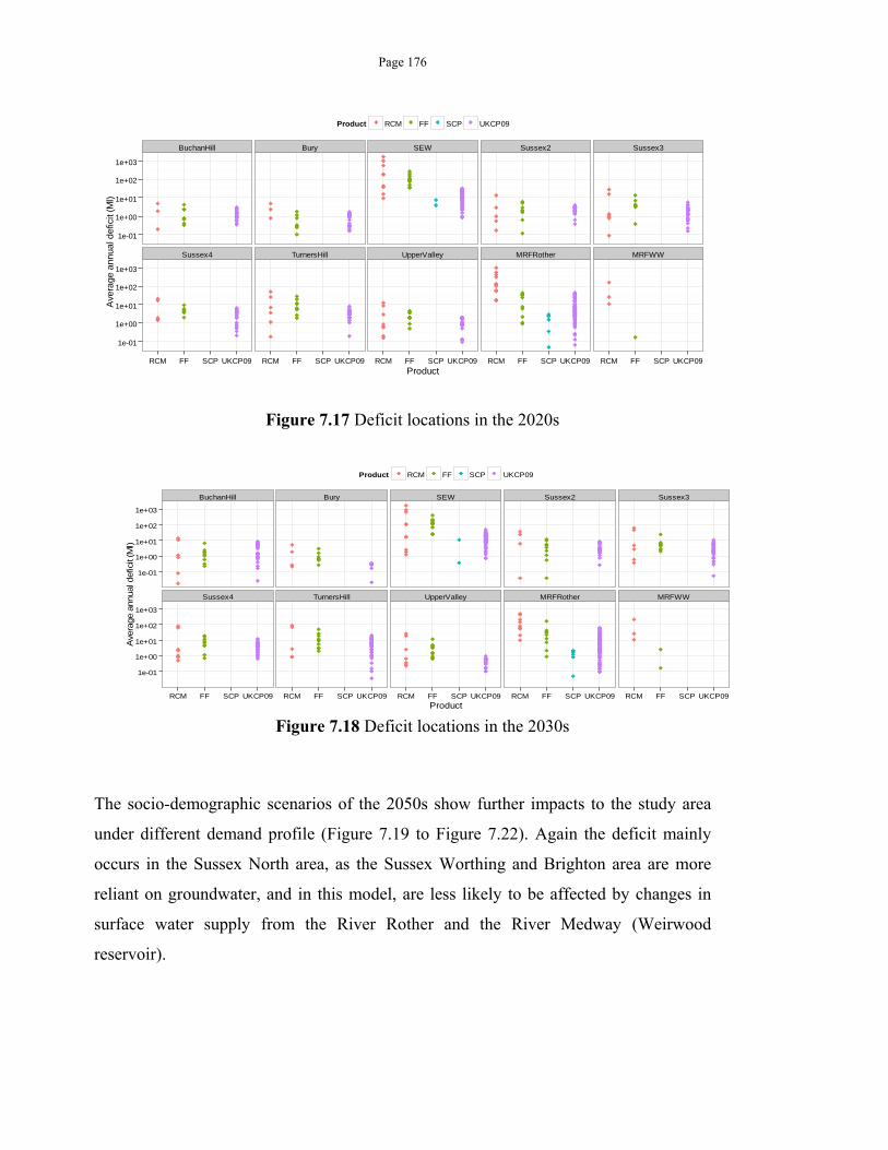
Page 176
Figure 7.17 Deficit locations in the 2020s
Figure 7.18 Deficit locations in the 2030s
The socio-demographic scenarios of the 2050s show further impacts to the study area
under different demand profile (Figure 7.19 to Figure 7.22). Again the deficit mainly
occurs in the Sussex North area, as the Sussex Worthing and Brighton area are more
reliant on groundwater, and in this model, are less likely to be affected by changes in
surface water supply from the River Rother and the River Medway (Weirwood
reservoir).
BuchanHill Bury SEW Sussex2 Sussex3
Sussex4 TurnersHill UpperValley MRFRother MRFWW
1e-01
1e+00
1e+01
1e+02
1e+03
1e-01
1e+00
1e+01
1e+02
1e+03
RCM FF SCP UKCP09 RCM FF SCP UKCP09 RCM FF SCP UKCP09 RCM FF SCP UKCP09 RCM FF SCP UKCP09Product
Ave
rage a
nnua
l defic
it (M
l)
Product RCM FF SCP UKCP09
BuchanHill Bury SEW Sussex2 Sussex3
Sussex4 TurnersHill UpperValley MRFRother MRFWW
1e-01
1e+00
1e+01
1e+02
1e+03
1e-01
1e+00
1e+01
1e+02
1e+03
RCM FF SCP UKCP09 RCM FF SCP UKCP09 RCM FF SCP UKCP09 RCM FF SCP UKCP09 RCM FF SCP UKCP09Product
Ave
rage a
nnual d
efic
it (M
l)
Product RCM FF SCP UKCP09
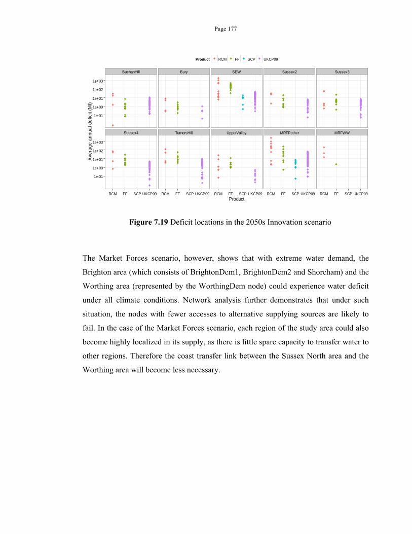
Page 177
Figure 7.19 Deficit locations in the 2050s Innovation scenario
The Market Forces scenario, however, shows that with extreme water demand, the
Brighton area (which consists of BrightonDem1, BrightonDem2 and Shoreham) and the
Worthing area (represented by the WorthingDem node) could experience water deficit
under all climate conditions. Network analysis further demonstrates that under such
situation, the nodes with fewer accesses to alternative supplying sources are likely to
fail. In the case of the Market Forces scenario, each region of the study area could also
become highly localized in its supply, as there is little spare capacity to transfer water to
other regions. Therefore the coast transfer link between the Sussex North area and the
Worthing area will become less necessary.
BuchanHill Bury SEW Sussex2 Sussex3
Sussex4 TurnersHill UpperValley MRFRother MRFWW
1e-01
1e+00
1e+01
1e+02
1e+03
1e-01
1e+00
1e+01
1e+02
1e+03
RCM FF SCP UKCP09 RCM FF SCP UKCP09 RCM FF SCP UKCP09 RCM FF SCP UKCP09 RCM FF SCP UKCP09Product
Ave
rag
e a
nn
ua
l de
ficit
(Ml)
Product RCM FF SCP UKCP09
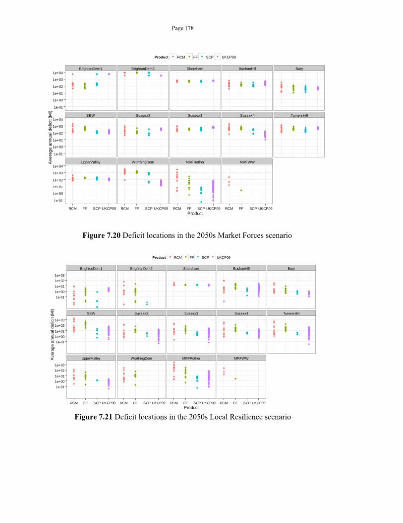
Page 178
Figure 7.20 Deficit locations in the 2050s Market Forces scenario
Figure 7.21 Deficit locations in the 2050s Local Resilience scenario
BrightonDem1 BrightonDem2 Shoreham BuchanHill Bury
SEW Sussex2 Sussex3 Sussex4 TurnersHill
UpperValley WorthingDem MRFRother MRFWW
1e-01
1e+00
1e+01
1e+02
1e+03
1e+04
1e-01
1e+00
1e+01
1e+02
1e+03
1e+04
1e-01
1e+00
1e+01
1e+02
1e+03
1e+04
RCM FF SCP UKCP09 RCM FF SCP UKCP09 RCM FF SCP UKCP09 RCM FF SCP UKCP09Product
Ave
rag
e a
nnu
al d
efic
it (M
l)
Product RCM FF SCP UKCP09
BrightonDem1 BrightonDem2 Shoreham BuchanHill Bury
SEW Sussex2 Sussex3 Sussex4 TurnersHill
UpperValley WorthingDem MRFRother MRFWW
1e-01
1e+00
1e+01
1e+02
1e+03
1e-01
1e+00
1e+01
1e+02
1e+03
1e-01
1e+00
1e+01
1e+02
1e+03
RCM FF SCP UKCP09 RCM FF SCP UKCP09 RCM FF SCP UKCP09 RCM FF SCP UKCP09Product
Ave
rag
e a
nn
ua
l de
ficit
(Ml)
Product RCM FF SCP UKCP09
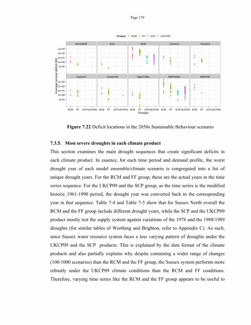
Page 179
Figure 7.22 Deficit locations in the 2050s Sustainable Behaviour scenario
7.3.5. Most severe droughts in each climate product
This section examines the main drought sequences that create significant deficits in
each climate product. In essence, for each time period and demand profile, the worst
drought year of each model ensemble/climate scenario is congregated into a list of
unique drought years. For the RCM and FF group, these are the actual years in the time
series sequence. For the UKCP09 and the SCP group, as the time series is the modified
historic 1961-1990 period, the drought year was converted back to the corresponding
year in that sequence. Table 7-4 and Table 7-5 show that for Sussex North overall the
RCM and the FF group include different drought years, while the SCP and the UKCP09
product mostly test the supply system against variations of the 1976 and the 1988/1989
droughts (for similar tables of Worthing and Brighton, refer to Appendix C). As such,
since Sussex water resource system faces a less varying pattern of droughts under the
UKCP09 and the SCP products. This is explained by the data format of the climate
products and also partially explains why despite containing a wider range of changes
(100/1000 scenarios) than the RCM and the FF group, the Sussex system performs more
robustly under the UKCP09 climate conditions than the RCM and FF conditions.
Therefore, varying time series like the RCM and the FF group appears to be useful to
BuchanHill Bury SEW Sussex2 Sussex3
Sussex4 TurnersHill UpperValley MRFRother MRFWW
1e-01
1e+00
1e+01
1e+02
1e+03
1e-01
1e+00
1e+01
1e+02
1e+03
RCM FF SCPUKCP09 RCM FF SCPUKCP09 RCM FF SCPUKCP09 RCM FF SCPUKCP09 RCM FF SCPUKCP09Product
Ave
rag
e a
nnu
al d
efic
it (M
l)
Product RCM FF SCP UKCP09
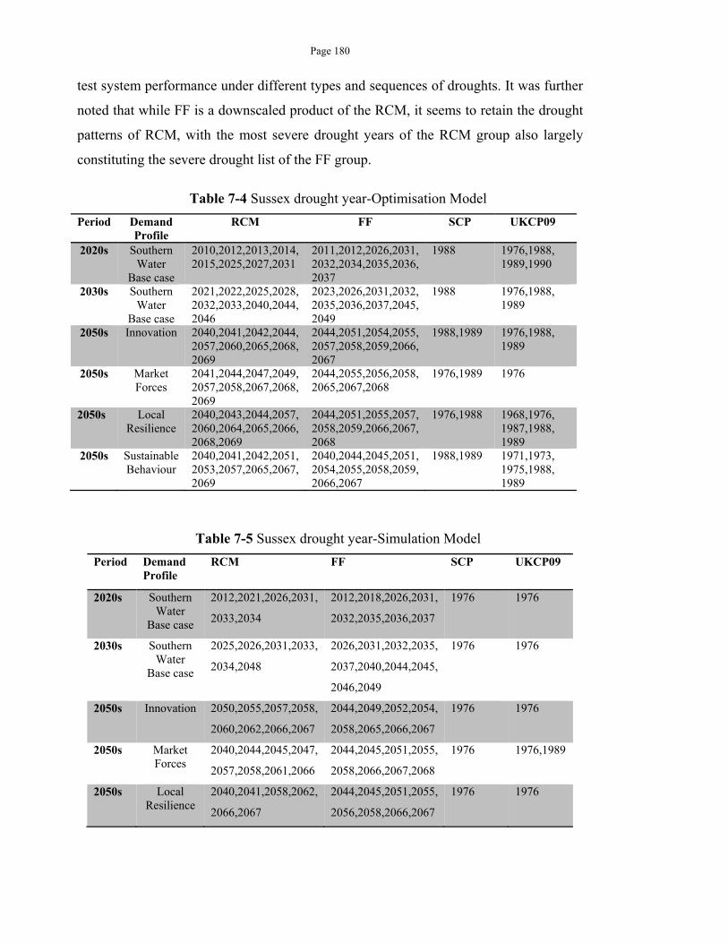
Page 180
test system performance under different types and sequences of droughts. It was further
noted that while FF is a downscaled product of the RCM, it seems to retain the drought
patterns of RCM, with the most severe drought years of the RCM group also largely
constituting the severe drought list of the FF group.
Table 7-4 Sussex drought year-Optimisation Model
Period Demand Profile
RCM FF SCP UKCP09
2020s Southern Water
Base case
2010,2012,2013,2014, 2015,2025,2027,2031
2011,2012,2026,2031, 2032,2034,2035,2036, 2037
1988
1976,1988, 1989,1990
2030s Southern Water
Base case
2021,2022,2025,2028, 2032,2033,2040,2044, 2046
2023,2026,2031,2032, 2035,2036,2037,2045, 2049
1988
1976,1988, 1989
2050s Innovation 2040,2041,2042,2044, 2057,2060,2065,2068, 2069
2044,2051,2054,2055, 2057,2058,2059,2066, 2067
1988,1989
1976,1988, 1989
2050s Market Forces
2041,2044,2047,2049, 2057,2058,2067,2068, 2069
2044,2055,2056,2058, 2065,2067,2068
1976,1989
1976
2050s Local Resilience
2040,2043,2044,2057, 2060,2064,2065,2066, 2068,2069
2044,2051,2055,2057, 2058,2059,2066,2067, 2068
1976,1988
1968,1976, 1987,1988, 1989
2050s Sustainable Behaviour
2040,2041,2042,2051, 2053,2057,2065,2067, 2069
2040,2044,2045,2051, 2054,2055,2058,2059, 2066,2067
1988,1989
1971,1973, 1975,1988, 1989
Table 7-5 Sussex drought year-Simulation Model
Period Demand Profile
RCM FF SCP UKCP09
2020s Southern Water
Base case
2012,2021,2026,2031,
2033,2034
2012,2018,2026,2031,
2032,2035,2036,2037
1976 1976
2030s Southern Water
Base case
2025,2026,2031,2033,
2034,2048
2026,2031,2032,2035,
2037,2040,2044,2045,
2046,2049
1976 1976
2050s Innovation 2050,2055,2057,2058,
2060,2062,2066,2067
2044,2049,2052,2054,
2058,2065,2066,2067
1976 1976
2050s Market Forces
2040,2044,2045,2047,
2057,2058,2061,2066
2044,2045,2051,2055,
2058,2066,2067,2068
1976 1976,1989
2050s Local Resilience
2040,2041,2058,2062,
2066,2067
2044,2045,2051,2055,
2056,2058,2066,2067
1976 1976
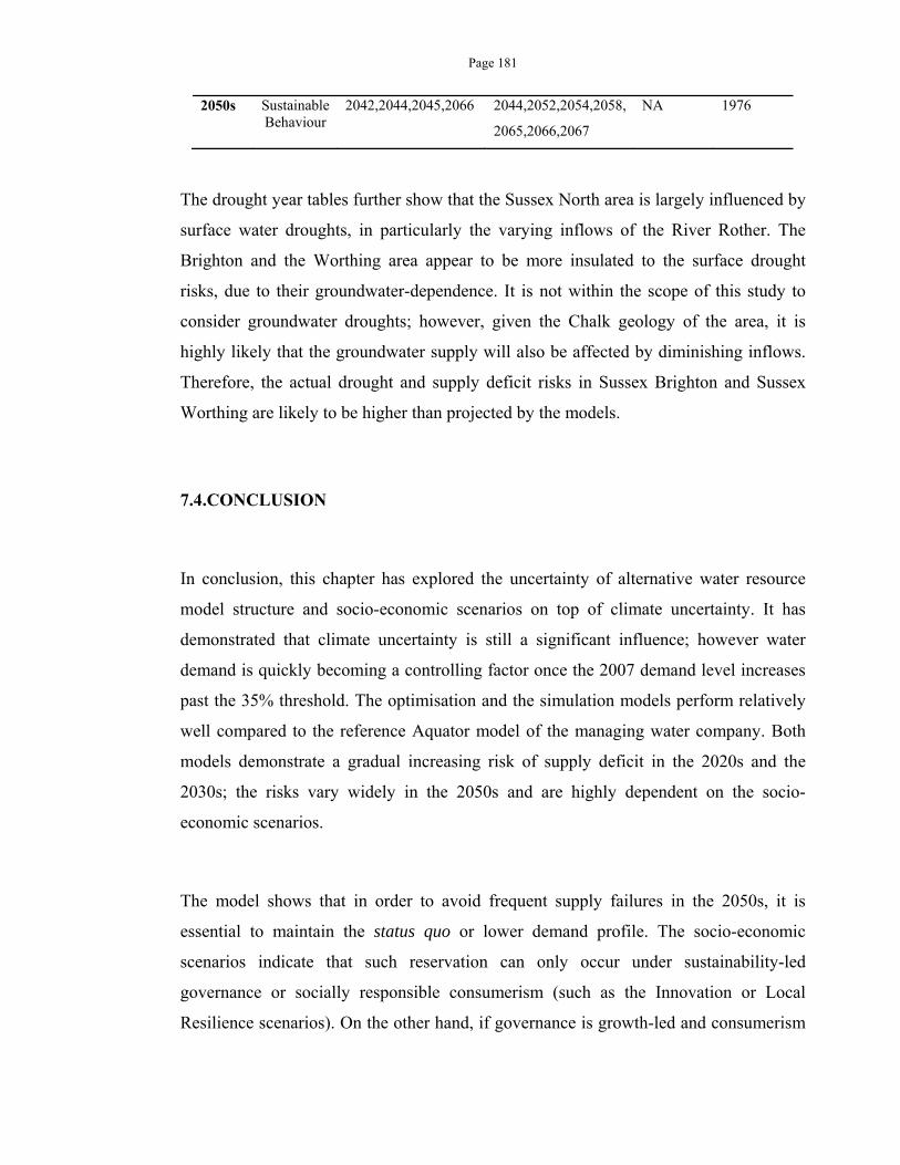
Page 181
2050s Sustainable Behaviour
2042,2044,2045,2066 2044,2052,2054,2058,
2065,2066,2067
NA 1976
The drought year tables further show that the Sussex North area is largely influenced by
surface water droughts, in particularly the varying inflows of the River Rother. The
Brighton and the Worthing area appear to be more insulated to the surface drought
risks, due to their groundwater-dependence. It is not within the scope of this study to
consider groundwater droughts; however, given the Chalk geology of the area, it is
highly likely that the groundwater supply will also be affected by diminishing inflows.
Therefore, the actual drought and supply deficit risks in Sussex Brighton and Sussex
Worthing are likely to be higher than projected by the models.
7.4.CONCLUSION
In conclusion, this chapter has explored the uncertainty of alternative water resource
model structure and socio-economic scenarios on top of climate uncertainty. It has
demonstrated that climate uncertainty is still a significant influence; however water
demand is quickly becoming a controlling factor once the 2007 demand level increases
past the 35% threshold. The optimisation and the simulation models perform relatively
well compared to the reference Aquator model of the managing water company. Both
models demonstrate a gradual increasing risk of supply deficit in the 2020s and the
2030s; the risks vary widely in the 2050s and are highly dependent on the socio-
economic scenarios.
The model shows that in order to avoid frequent supply failures in the 2050s, it is
essential to maintain the status quo or lower demand profile. The socio-economic
scenarios indicate that such reservation can only occur under sustainability-led
governance or socially responsible consumerism (such as the Innovation or Local
Resilience scenarios). On the other hand, if governance is growth-led and consumerism
Page 182
is individualistic, the system will face significantly high risks of water supply deficit to
all the areas. The models do not consider groundwater drought risks, which may affect
the groundwater-dependent Brighton and Worthing areas. Thus the future failure risks
are mainly distributed within the Sussex North area, with the exception of the Market
Forces scenario. However, given the Chalk geology of the area, it is likely that Brighton
and Worthing will experience supply deficit during prolonged surface water droughts.
Finally, the cross-climate product analysis shows that the Sussex system is relatively
robust under different variations of the 1975/1976 and the 1988/1989 droughts, possibly
due to the usage of these historic event as the design event of drought planning. The
system, however, is less immune to other, potentially new, sequence of droughts as
projected in the RCM and the FF group. While the FF group is a downscaled and bias-
corrected product of the RCM ensembles, its impacts on water deficits are quite similar
to the RCM groups, which are much drier time series. The system is overall sensitive to
the actual sequence of droughts and the low flow levels. It is therefore suggested that
while UKCP09 contains the most wide ranging climatic conditions and possible
changes, the actual historic-based application of the product limits its utility in testing
system robustness. Therefore, aside from exploring alternative scenarios (as suggested
in the Robust Decision Making framework), time series with diverse patterns are highly
useful to test the system against surprise, particularly with regard to climate risks.
Page 183
Chapter 8. WATER RESOURCE PLANNING UNDER UNCERTAINTY
8.1.INTRODUCTION
In the previous chapter, the vulnerability of the study area was explored under different
demand and climate scenarios. Overall the area appears to be under various stresses, of
which climate uncertainty and demand uncertainty are two influential ones. This chapter
proceeds by analysing selected planning options of the area, and whether those options
can accommodate the water demand of the area. It continues to follow the cascade of
uncertainty as explored in previous chapters by using the four climate products as the
inputs of a water resource planning system. Additionally, for the 2050s, it considers
four alternative socio-economic scenarios leading to different levels of water demand.
The chapter will mainly focus on the technical aspects of Decision Support System for
decisions under uncertainty; further implications of the results on policy and
adaptability of water resources planning to new patterns of risks will be discussed in
detail in Chapter 9. First, Section 8.2 will describe the options and how they are
analysed in the optimisation model. Second, Section 8.3 then presents and discusses the
results, with in-depth analysis of the delivery network and the effectiveness of options
in reducing supply vulnerability.
Planning decisions under the deep uncertainty of climate change and demand
uncertainty is highly difficult. Arnell and Delaney (2006) outlined this adaptation
process by four key points: impact awareness and concern, adaptation strategy, option
selection and the influence of changes in the organisation characteristics, the regulation
and the market on these factors. In the context of the UK, as described in Chapter 4, it
involves revising a 25-year water resource plan, revised every five years. The focus of
the plan, as typical of planning problems, does not only revolve just around the climate
impacts; rather, it has to deal with a combination of stressors including water demand
Page 184
growth, supply reliability and the other socio-economic changes. Indeed, water demand
management one of the core elements for water management to test the system
robustness and reliability (Baumann et al., 1997; Butler and Memon, 2006). For water
management in England and Wales, the headroom concept, the extra water supply
capacity to accommodate unplanned demand, is often used in these plans to ensure
system reliability and robustness. Based on these projected demand profiles, the water
companies analyse their available options and select options to consider for the future.
Apart from the UKCP02 and subsequently UKCP09 climate product, other products
such as the Weather Generator, multi-model ensembles and Future Flows have also
been used for risk analysis (Fowler et al., 2003; Christensen and Lettenmaier, 2006;
Wilby and Harris, 2006; Fowler et al., 2007; Lopez et al., 2009b; Prudhomme and
Davies, 2009). Many studies treat adaptation of the water planning system as a case of
capacity expansion that accommodate the most likely projected demand (Jenkins et al.,
2004; O’Hara and Georgakakos, 2008). Others like Lempert and Schlesinger (2000) and
Wilby and Dessai () criticised this ‘predict-then-act’ approach and advocated a robust
adaptation approach which considers all possible uncertainty and imaginable futures.
There have been various methods of constructing the scenarios and time series. Lempert
and Groves (2010) have used qualitatively different scenarios to test the robustness of
water planning options under deep uncertainty. Paton et al. (2013) employed stochastic
rainfall time series constructed from historical records while Manning et al. (2009) used
the Bayesian statistical approach to construct the probability distribution of local
climate change which provide the Thames catchment rainfall-runoff model with inputs
to simulate future water abstraction availability. Yet, while the probabilistic approach
can facilitate a risk-based assessment framework, New et al. (2007) argued that climate
risks will change over time; similarly, Hall et al. (2007) stated that probabilistic climate
scenarios may misrepresent uncertainty.
In terms of model choices, both optimization and simulation models have been used,
such as AQUASIM (Huggenberger et al., 2013), IRAS (Matrosov et al., 2013),
Watersim (Gober et al., 2010), Watercress (Paton et al., 2013). As discussed in Chapter
3, water resource planning can be formulated as a decision analysis problem in which
Page 185
the outcomes are selected on an optimisation or a satisficing basis. Alternatively,
strategies can be selected via the use of simulation models, which follow operating rules
specified by the users. These simulation models will then test the system and various
strategies under the scenarios; via those tests, the users can analyse system performance
based on their criteria and decide on the planning strategies. For adaptation under
uncertainty, both the optimisation and the simulation approaches have been used to
identify system vulnerability and robust strategies under varying conditions. The
number of simulations tends to grow larger with the complexity of the model; on the
other hand, the number of optimisation runs does not grow at the same order but the
searching time may be prolonged due to the increasingly complexity of the response
surface. Kasprzyk et al. (2012) further combined Sobol’s variance decomposition with
multi-objective evolutionary algorithms to generate the testing scenario and analyse
system robustness. Meanwhile Matrosov et al. (2011) used a simulation model to test
the conjunctive use of the Thames water resource system and Matrosov et al. (2013)
compared an optimised plan with a Robust Decision Making plan to highlight the
differences of these two approaches. However, to date, option analysis in water
management and planning in England and Wales is still often separated from water
resource modelling. Instead, the options are selected in a separate investment model
which considers the average contribution to supply, financial investment and
operational cost as well as the implementation duration. An integrated investment-water
resource model is necessary since the actual supply of the option or demand reduction
effects are dependent on the water supply network, as well as the nature of the supply
deficits.
Based on that context, this chapter presents an example of using the optimisation model
to select options based on the criteria of maintaining the minimum environmental flows
and abating supply deficits with minimum operational cost. Firstly, Section 8.2
describes how the planning options were implemented in the simulation and
optimisation model described in Chapter 7. It then outlines the planning options
considered in the study and criteria for planning success. Secondly, Section 8.3 presents
the option selected by the optimisation model, their comparative performance by the
Page 186
simulation model and the remaining vulnerability of the Sussex area under these plans.
Section 8.4 then concludes with key points and results of the chapter.
8.2.METHODOLOGY
8.2.1. Problem formulation
In order to construct a Decision Support System for the study area, the problem is
formulated as planning for a water supply network under climate change impacts. Due
to changes in surface inflows, the region has to invest on strategies that augment supply,
reduce demand or enhance transferring capacity. The study uses the optimisation model,
a mathematical model which minimizes three criteria: total deficit in demand nodes,
total deficit in environmental flows and the total financial cost of maintaining the best-
possible water supply-demand balance. The problem is formulated as a mixed integer
linear programming problem, with core decision variables of interest being binary
variables that represents whether a strategy should be implemented or not.
The model is divided into two parts: a core model that represents physical relations
between variables and a preferential model that searches for solutions based on the
criterion preferences.
8.2.2. Core model specification
A core model usually contains given parameters, state variables, decision variables and
constraints. In this study, as the focus is on a water supply network, the core model
takes the form of a flow network that delivers water from sources to sinks. The model is
formulated as a linear programming of which decision variables are not related via
multiplication or division. For specific equations of the model, please refer to Appendix
A.
Page 187
8.2.3. Strategy representation
Planning strategies are represented as binary decision variable Xi (t) that will take the
value of 1 if implemented during the time step t and 0 otherwise. Once implemented,
the binary variable Use(Xi,t) presents whether the strategy is actually used, for instance
in a time step if a desalination plant may have been implemented but does not supply
water to the network, it will have XDesal=1 and Use(XDesal)=0. Effects of the strategy
onto the network include supply augmentation, demand reduction and changes on
transfer capacity. Furthermore, options can be mutually exclusive, such as the
implementation of one option will exclude another option, or have interactive effects.
Decision variables that can provide additional supply are modelled as a fictional source
that is not connected to other sources if the strategy is not implemented. This setup also
allows calculating the real usage of the option (e.g. the supply provided by the decision
variable and the frequency of source usage). Based on Southern Water 2009 Water
Resource Management Plan, nine potential strategies were included in the model (Table
8-1). Strategies are characterized into non-permanent and permanent options: the former
can be turned off once not needed (such as hosepipe ban measures) while the latter
remains in place once implemented and incurs fixed operational cost even when they
are not used. Strategies are also grouped into groups of mutually exclusive options.
Hosepipe bans are governed by the rainfall-based SPI12. In essence, the model can
choose to implement hosepipe ban up to 10% of the whole time series in time steps with
SPI12 < -1.8. This condition was based on the Drought Plan of the study area (Southern
Water, 2013).
Taking supply from supply nodes would incur a pumping cost, as described in Chapter
7. The cost is different for each source, which reflects their priority of abstraction and
the actual financial cost. To avoid double counting, the pumping cost is only accounted
in the immediate links to the source. Overall, surface water from River Rother would be
the first supply source, followed by other groundwater (except Hardham) sources. Note
that this is not the accurate pumping price; it was constructed to be similar to the real
cost, but also the pumping priority of the source nodes. With nodes and links that can be
modified by the Decision Variables, the cost includes additional operational cost
Page 188
(OPEX) of the implemented strategies. Once an option is implemented, the cost also
includes a one-off capital investment cost (CAPEX). All the pumping cost, OPEX and
CAPEX are adjusted using a discount rate based on the Treasury Green book (Her
Majesty’s Treasury, 2013) of 5%. As such, the same amount of money in a later time
step will have a lower cost than it is in an earlier time step.
1
Equation 8-1
in which n is the year of the time series, NPV is the Net Present Value and p is the
discount rate
Therefore, the model will implement and activate strategies as later as possible, unless
to mitigate deficits.
As described in Chapter 4, the study area consists of Sussex North, Sussex Worthing
and Sussex Brighton. It has two inter-company water transfers: Southern Water
provides South East Water with 5.4 Ml/day from the Weirwood Reservoir for and can
receive up to 15 Ml/d from Portsmouth Water to the Hardham WSW. The V6
bidirectional link between Sussex North and Sussex Worthing can transfer up to 15
Ml/d in either direction while the Rockroad link from Worthing to Brighton can
distribute up to 7 Ml/d. Under situation of water shortages, the available supply
therefore can be transferred between Worthing and Sussex North, as well as from either
of these zones to Brighton.
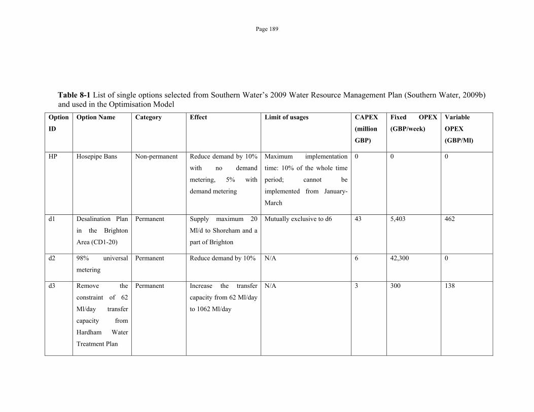
Page 189
Table 8-1 List of single options selected from Southern Water’s 2009 Water Resource Management Plan (Southern Water, 2009b) and used in the Optimisation Model
Option
ID
Option Name Category Effect Limit of usages CAPEX
(million
GBP)
Fixed OPEX
(GBP/week)
Variable
OPEX
(GBP/Ml)
HP Hosepipe Bans Non-permanent Reduce demand by 10%
with no demand
metering, 5% with
demand metering
Maximum implementation
time: 10% of the whole time
period; cannot be
implemented from January-
March
0 0 0
d1 Desalination Plan
in the Brighton
Area (CD1-20)
Permanent Supply maximum 20
Ml/d to Shoreham and a
part of Brighton
Mutually exclusive to d6 43 5,403 462
d2 98% universal
metering
Permanent Reduce demand by 10% N/A 6 42,300 0
d3 Remove the
constraint of 62
Ml/day transfer
capacity from
Hardham Water
Treatment Plan
Permanent Increase the transfer
capacity from 62 Ml/day
to 1062 Ml/day
N/A 3 300 138
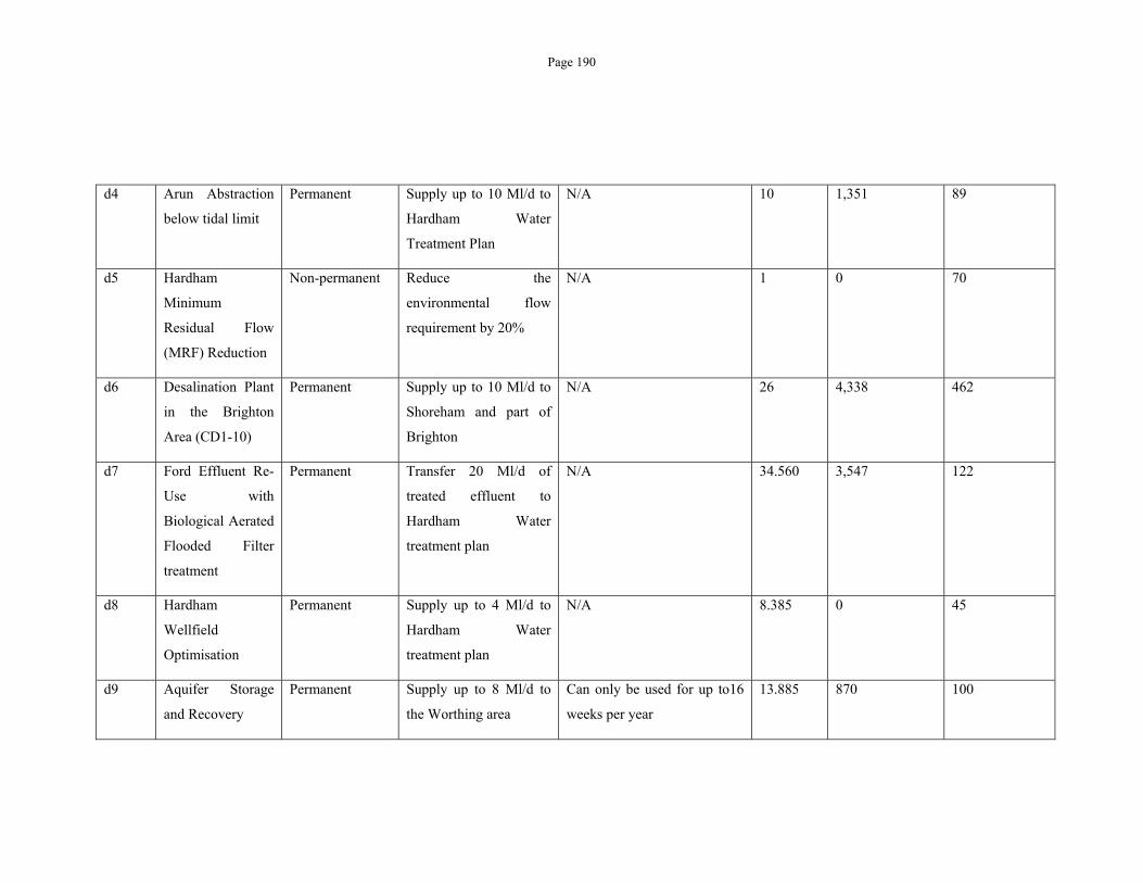
Page 190
d4 Arun Abstraction
below tidal limit
Permanent Supply up to 10 Ml/d to
Hardham Water
Treatment Plan
N/A 10 1,351 89
d5 Hardham
Minimum
Residual Flow
(MRF) Reduction
Non-permanent Reduce the
environmental flow
requirement by 20%
N/A 1 0 70
d6 Desalination Plant
in the Brighton
Area (CD1-10)
Permanent Supply up to 10 Ml/d to
Shoreham and part of
Brighton
N/A 26 4,338 462
d7 Ford Effluent Re-
Use with
Biological Aerated
Flooded Filter
treatment
Permanent Transfer 20 Ml/d of
treated effluent to
Hardham Water
treatment plan
N/A 34.560 3,547 122
d8 Hardham
Wellfield
Optimisation
Permanent Supply up to 4 Ml/d to
Hardham Water
treatment plan
N/A 8.385 0 45
d9 Aquifer Storage
and Recovery
Permanent Supply up to 8 Ml/d to
the Worthing area
Can only be used for up to16
weeks per year
13.885 870 100
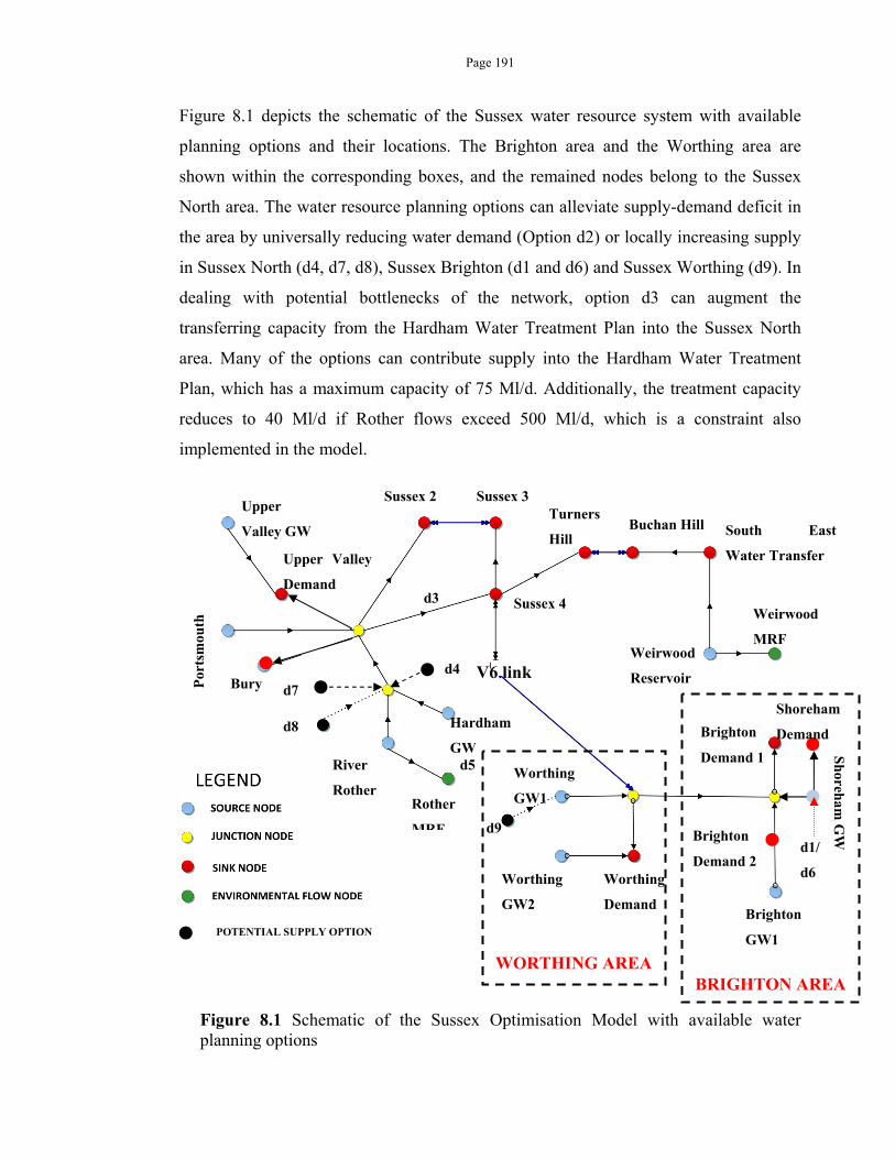
Page 191
Figure 8.1 depicts the schematic of the Sussex water resource system with available
planning options and their locations. The Brighton area and the Worthing area are
shown within the corresponding boxes, and the remained nodes belong to the Sussex
North area. The water resource planning options can alleviate supply-demand deficit in
the area by universally reducing water demand (Option d2) or locally increasing supply
in Sussex North (d4, d7, d8), Sussex Brighton (d1 and d6) and Sussex Worthing (d9). In
dealing with potential bottlenecks of the network, option d3 can augment the
transferring capacity from the Hardham Water Treatment Plan into the Sussex North
area. Many of the options can contribute supply into the Hardham Water Treatment
Plan, which has a maximum capacity of 75 Ml/d. Additionally, the treatment capacity
reduces to 40 Ml/d if Rother flows exceed 500 Ml/d, which is a constraint also
implemented in the model.
Figure 8.1 Schematic of the Sussex Optimisation Model with available water planning options
d1/
d6
d3
d4
d8
d7
Weirwood
Reservoir
Weirwood
MRF
South East
Water Transfer
Brighton
GW1
Sh
oreham
GW
Worthing
Demand
Worthing
GW2
Worthing
GW1
d9
Upper
Valley GW
Upper Valley
Demand
Sussex 2 Sussex 3
Sussex 4
Por
tsm
outh
Rother
MRF
River
Rother
Hardham
GWd5
Brighton
Demand 2
Brighton
Demand 1
Turners
Hill Buchan Hill
Bury
Shoreham
Demand
WORTHING AREA
BRIGHTON AREA
V6 link
POTENTIAL SUPPLY OPTION
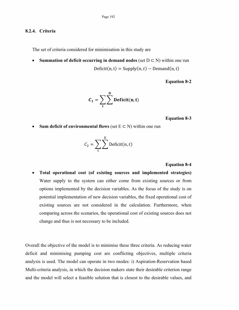
Page 192
8.2.4. Criteria
The set of criteria considered for minimisation in this study are
Summation of deficit occurring in demand nodes (set D ⊂ N) within one run
De icit n, t Supply , Demand n, t
Equation 8-2
,
Equation 8-3
Sum deficit of environmental flows (set E ⊂ N) within one run
De icit ,
Equation 8-4
Total operational cost (of existing sources and implemented strategies)
Water supply to the system can either come from existing sources or from
options implemented by the decision variables. As the focus of the study is on
potential implementation of new decision variables, the fixed operational cost of
existing sources are not considered in the calculation. Furthermore, when
comparing across the scenarios, the operational cost of existing sources does not
change and thus is not necessary to be included.
Overall the objective of the model is to minimise these three criteria. As reducing water
deficit and minimising pumping cost are conflicting objectives, multiple criteria
analysis is used. The model can operate in two modes: i) Aspiration-Reservation based
Multi-criteria analysis, in which the decision makers state their desirable criterion range
and the model will select a feasible solution that is closest to the desirable values, and
Page 193
ii) Ranked Optimisation, in which the model optimises from the most prioritised
criterion to other criteria. As described in Chapter 7, expert judgement by relevant
decision makers indicated a preference for the latter method. Therefore this chapter
continued to use the second mode to select the preferred planning option for each
scenario. In particular, the model first minimises possible environmental flow deficits,
then reruns with that minimum value to search for the minimum possible demand
deficits. It is thus a process of selecting from multiple options with the minimum
environment flow deficits, then choosing amongst them for ones with the minimum
demand deficit and then selecting the one with the least cost. Finally the model searches
for a solution with minimum overall cost while maintaining that minimum deficits on
environmental flows and demand.
8.2.5. Scenarios
The scenarios follow those of Chapter 7, which uses four different climate products and
socio-economic scenarios from Southern Water and the EA. Additionally, for each
scenario, the testing set will include a headroom demand uncertainty, in which non-
environmental demand is increased by 5%, and a headroom demand-groundwater
outage uncertainty, in which the demand is at the headroom level and groundwater
supply is reduced by 5% due to outages.
8.2.6. Robust Decision Analysis using the Simulation Model
Due to the time and computational constraints, the study could not use the Simulation
Model to analyse the 512 possible sets of options. Therefore, the Optimisation Model
was used to reduce the number of options. In this step, all options selected by the
Optimisation Model in the 2020s, 2030s and 2050s for each demand scenario will be
rerun by the Simulation Model. This produces a basis for comparison of sub-optimal
options overall, to identify the other potentially robust packages of options that can
satisfy the acceptable level of cost and supply deficit. Analysis of the whole packages
rather than selecting the optimal option for the majority of scenarios will reduce the
Page 194
risks of selecting non-robust options. This approach has been described in more detail in
Chapter 3, in particular Section 3.2.
8.3.RESULTS AND DISCUSSION
8.3.1. Option Selection
The results show that using the potential options under optimisation, the system can
successfully cope with the demand increase. Since none of the options can augment the
environmental flows, the values of the environmental flows remain the same as in
Chapter 7 (refer to Figure 7.16a). In terms of deficit, Figure 8.2 depicts that under the
Base case, supply deficit of even the most extreme 2050s socio-economic scenario- the
Market Forces scenario-still remains similar to that of other 2050s demand scenarios.
The major variation of average annual deficit occurs across different climate products,
and as such depicts that climate post-processing is the major uncertainty factor in the
uncertainty cascade under the Base Case socio-economic scenario.
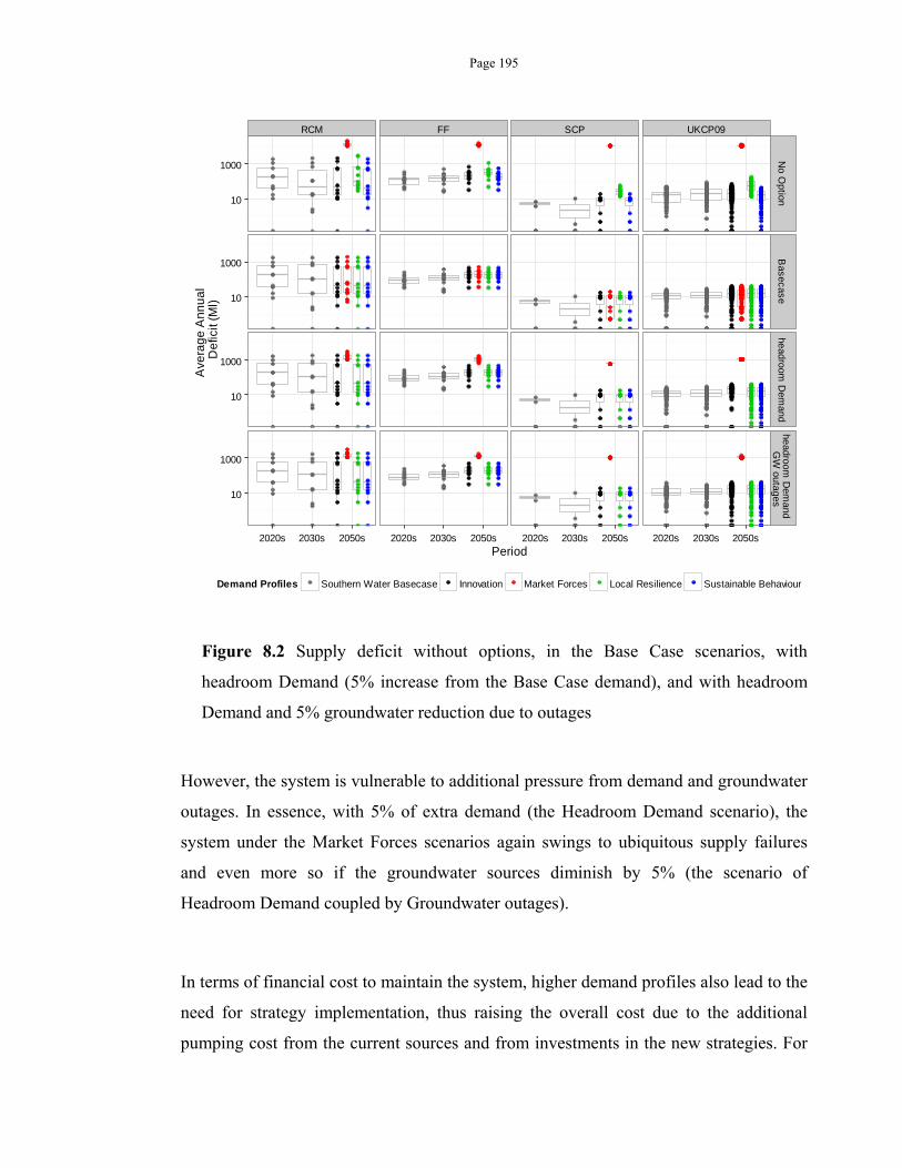
Page 195
Figure 8.2 Supply deficit without options, in the Base Case scenarios, with
headroom Demand (5% increase from the Base Case demand), and with headroom
Demand and 5% groundwater reduction due to outages
However, the system is vulnerable to additional pressure from demand and groundwater
outages. In essence, with 5% of extra demand (the Headroom Demand scenario), the
system under the Market Forces scenarios again swings to ubiquitous supply failures
and even more so if the groundwater sources diminish by 5% (the scenario of
Headroom Demand coupled by Groundwater outages).
In terms of financial cost to maintain the system, higher demand profiles also lead to the
need for strategy implementation, thus raising the overall cost due to the additional
pumping cost from the current sources and from investments in the new strategies. For
RCM FF SCP UKCP09
10
1000
10
1000
10
1000
10
1000
No O
ptionB
asecaseheadroom
Dem
andheadroom
Dem
and G
W outages
2020s 2030s 2050s 2020s 2030s 2050s 2020s 2030s 2050s 2020s 2030s 2050sPeriod
Ave
rag
e A
nn
ua
l D
efic
it (M
l)
Demand Profiles Southern Water Basecase Innovation Market Forces Local Resilience Sustainable Behaviour
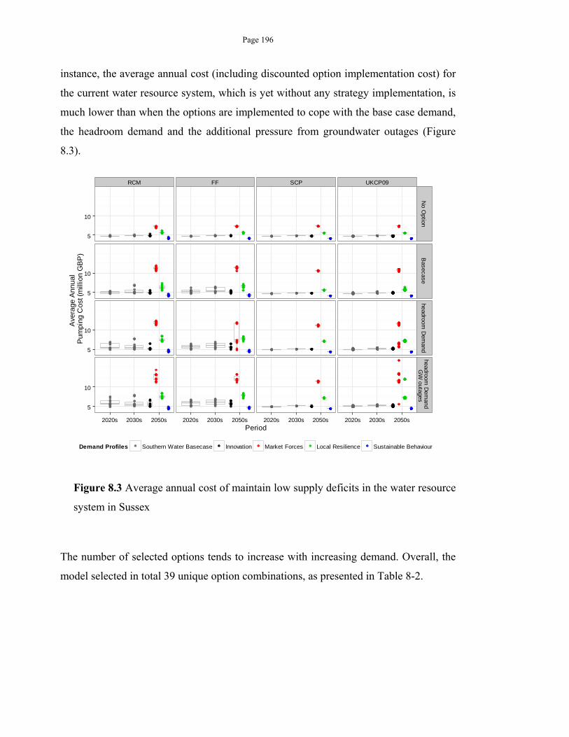
Page 196
instance, the average annual cost (including discounted option implementation cost) for
the current water resource system, which is yet without any strategy implementation, is
much lower than when the options are implemented to cope with the base case demand,
the headroom demand and the additional pressure from groundwater outages (Figure
8.3).
Figure 8.3 Average annual cost of maintain low supply deficits in the water resource
system in Sussex
The number of selected options tends to increase with increasing demand. Overall, the
model selected in total 39 unique option combinations, as presented in Table 8-2.
RCM FF SCP UKCP09
5
10
5
10
5
10
5
10
No O
ptionB
asecaseheadroom
Dem
andheadroom
Dem
and G
W outages
2020s 2030s 2050s 2020s 2030s 2050s 2020s 2030s 2050s 2020s 2030s 2050sPeriod
Ave
rage
Annual
Pum
ping
Cos
t (m
illio
n G
BP
)
Demand Profiles Southern Water Basecase Innovation Market Forces Local Resilience Sustainable Behaviour
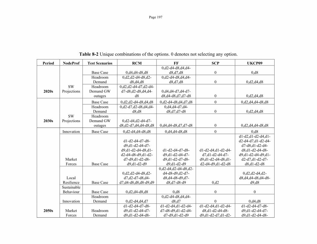
Page 197
Table 8-2 Unique combinations of the options. 0 denotes not selecting any option.
Period NodeProf Test Scenarios RCM FF SCP UKCP09
2020s
SW Projections
Base Case 0,d4,d4-d8,d8 0,d2-d4-d8,d4,d4-
d8,d7,d8 0 0,d8 Headroom Demand
0,d2,d2-d4-d8,d2-d8,d4,d8
0,d2-d4-d8,d4,d4-d8,d7,d8 0 0,d2,d4,d8
Headroom Demand GW
outages
0,d2,d2-d4-d7,d2-d4-d7-d8,d2-d8,d4,d4-
d8 0,d4,d4-d7,d4-d7-d8,d4-d8,d7,d7-d8 0 0,d2,d4,d8
2030s
SW Projections
Base Case 0,d2,d2-d4-d8,d4,d8 0,d2-d4-d8,d4,d7,d8 0 0,d2,d4,d4-d8,d8 Headroom Demand
0,d2-d7,d2-d8,d4,d4-d8,d8
0,d4,d4-d7,d4-d8,d7,d7-d8 0 0,d2,d4,d8
Headroom Demand GW
outages 0,d2-d4,d2-d4-d7-
d8,d2-d7,d4,d4-d8,d8 0,d4,d4-d8,d7,d7-d8 0 0,d2,d4,d4-d8,d8
2050s
Innovation Base Case 0,d2-d4,d4-d8,d8 0,d4,d4-d8,d8 0 0,d8
Market Forces Base Case
d1-d2-d4-d7-d8-d9,d1-d2-d4-d7-
d9,d1-d2-d4-d8,d1-d2-d4-d8-d9,d1-d2-
d7-d9,d1-d2-d8-d9,d1-d2-d9
d1-d2-d4-d7-d8-d9,d1-d2-d4-d7-d9,d1-d2-d7-d8-
d9,d1-d2-d9
d1-d2-d4,d1-d2-d4-d7,d1-d2-d4-d7-
d9,d1-d2-d4-d8,d1-d2-d4-d9,d1-d2-d8
d1-d2,d1-d2-d4,d1-d2-d4-d7,d1-d2-d4-
d7-d8,d1-d2-d4-d8,d1-d2-d4-d8-
d9,d1-d2-d4-d9,d1-d2-d7,d1-d2-d7-
d8,d1-d2-d8
Local Resilience Base Case
0,d2,d2-d4-d8,d2-d7,d2-d7-d8,d4-
d7,d4-d8,d8,d8-d9,d9
0,d2-d4,d2-d4-d8,d2-d4-d8-d9,d2-d7-d8,d4-d8-d9,d7-
d8,d7-d8-d9 0,d2
0,d2,d2-d4,d2-d8,d4,d4-d8,d4-d8-
d9,d8 Sustainable Behaviour Base Case 0,d2,d4-d8,d8 0,d8 0 0
Innovation Headroom Demand 0,d2-d4,d4,d7
0,d2-d4-d8,d4,d4-d8,d7 0 0,d4,d8
Market Forces
Headroom Demand
d1-d2-d4-d7-d8-d9,d1-d2-d4-d7-d9,d1-d2-d4-d8-
d1-d2-d4,d1-d2-d4-d7-d8-d9,d1-d2-d4-
d7-d9,d1-d2-d9
d1-d2-d4,d1-d2-d4-d8,d1-d2-d4-d8-
d9,d1-d2-d7,d1-d2-
d1-d2-d4-d7-d8-d9,d1-d2-d4-d7-d9,d1-d2-d4-d8-
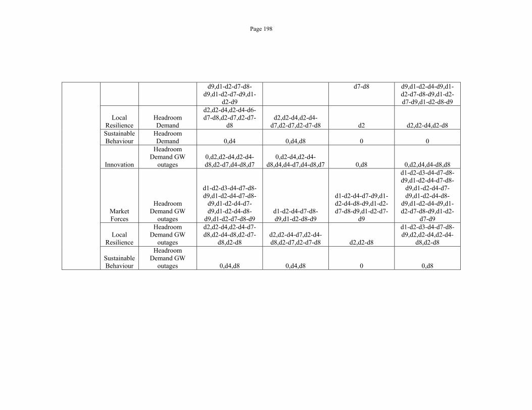
Page 198
d9,d1-d2-d7-d8-d9,d1-d2-d7-d9,d1-
d2-d9
d7-d8 d9,d1-d2-d4-d9,d1-d2-d7-d8-d9,d1-d2-d7-d9,d1-d2-d8-d9
Local Resilience
Headroom Demand
d2,d2-d4,d2-d4-d6-d7-d8,d2-d7,d2-d7-
d8 d2,d2-d4,d2-d4-
d7,d2-d7,d2-d7-d8 d2 d2,d2-d4,d2-d8 Sustainable Behaviour
Headroom Demand 0,d4 0,d4,d8 0 0
Innovation
Headroom Demand GW
outages 0,d2,d2-d4,d2-d4-d8,d2-d7,d4-d8,d7
0,d2-d4,d2-d4-d8,d4,d4-d7,d4-d8,d7 0,d8 0,d2,d4,d4-d8,d8
Market Forces
Headroom Demand GW
outages
d1-d2-d3-d4-d7-d8-d9,d1-d2-d4-d7-d8-
d9,d1-d2-d4-d7-d9,d1-d2-d4-d8-
d9,d1-d2-d7-d8-d9 d1-d2-d4-d7-d8-d9,d1-d2-d8-d9
d1-d2-d4-d7-d9,d1-d2-d4-d8-d9,d1-d2-d7-d8-d9,d1-d2-d7-
d9
d1-d2-d3-d4-d7-d8-d9,d1-d2-d4-d7-d8-
d9,d1-d2-d4-d7-d9,d1-d2-d4-d8-
d9,d1-d2-d4-d9,d1-d2-d7-d8-d9,d1-d2-
d7-d9
Local Resilience
Headroom Demand GW
outages
d2,d2-d4,d2-d4-d7-d8,d2-d4-d8,d2-d7-
d8,d2-d8 d2,d2-d4-d7,d2-d4-d8,d2-d7,d2-d7-d8 d2,d2-d8
d1-d2-d3-d4-d7-d8-d9,d2,d2-d4,d2-d4-
d8,d2-d8
Sustainable Behaviour
Headroom Demand GW
outages 0,d4,d8 0,d4,d8 0 0,d8
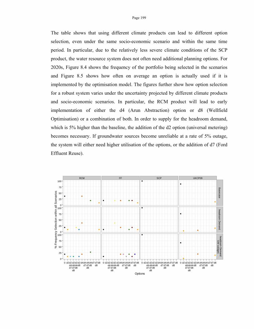
Page 199
The table shows that using different climate products can lead to different option
selection, even under the same socio-economic scenario and within the same time
period. In particular, due to the relatively less severe climate conditions of the SCP
product, the water resource system does not often need additional planning options. For
2020s, Figure 8.4 shows the frequency of the portfolio being selected in the scenarios
and Figure 8.5 shows how often on average an option is actually used if it is
implemented by the optimisation model. The figures further show how option selection
for a robust system varies under the uncertainty projected by different climate products
and socio-economic scenarios. In particular, the RCM product will lead to early
implementation of either the d4 (Arun Abstraction) option or d8 (Wellfield
Optimisation) or a combination of both. In order to supply for the headroom demand,
which is 5% higher than the baseline, the addition of the d2 option (universal metering)
becomes necessary. If groundwater sources become unreliable at a rate of 5% outage,
the system will either need higher utilisation of the options, or the addition of d7 (Ford
Effluent Reuse).
RCM FF SCP UKCP09
0
25
50
75
100
0
25
50
75
100
0
25
50
75
100
Basecase
headroom D
emand
headroom D
emand
GW
outages
0 d2d2d4d7
d2d4d7d8
d2d4d8
d2d8
d4d4d7
d4d7d8
d4d8
d7d7d8
d8 0 d2d2d4d7
d2d4d7d8
d2d4d8
d2d8
d4d4d7
d4d7d8
d4d8
d7d7d8
d8 0 d2d2d4d7
d2d4d7d8
d2d4d8
d2d8
d4d4d7
d4d7d8
d4d8
d7d7d8
d8 0 d2d2d4d7
d2d4d7d8
d2d4d8
d2d8
d4d4d7
d4d7d8
d4d8
d7d7d8
d8
Options
% F
requ
enc
y S
ele
ctio
n w
ithin
all
Sce
nar
ios
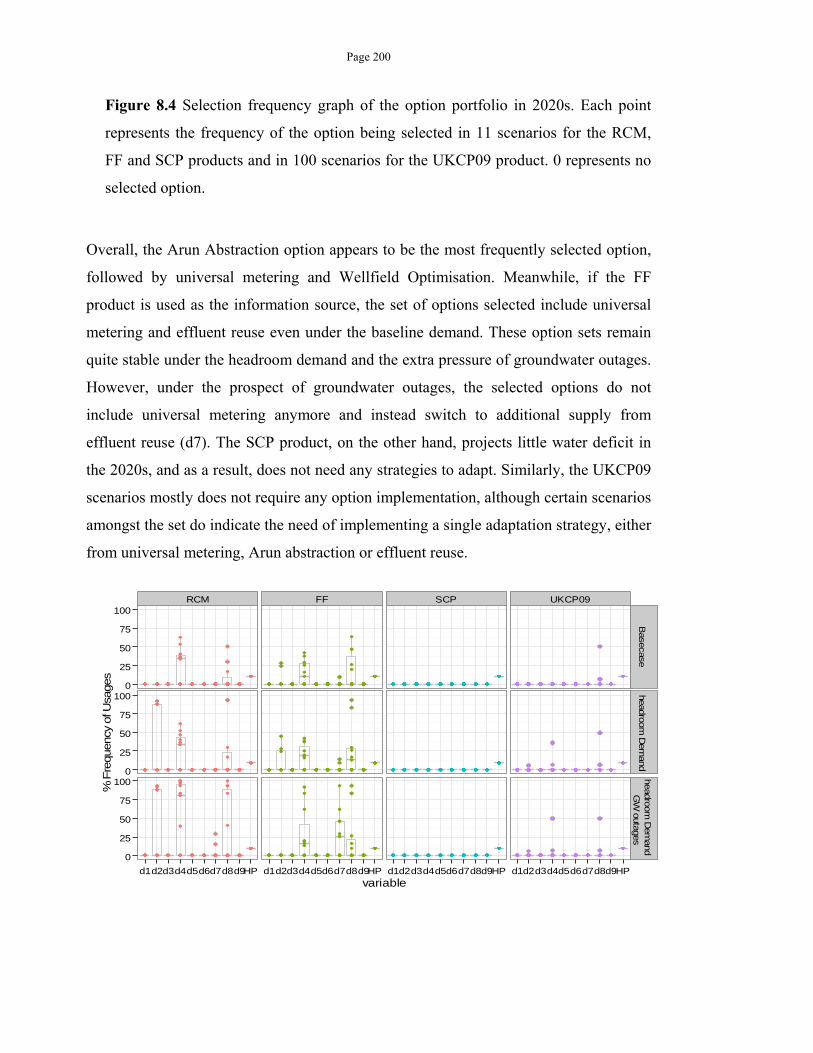
Page 200
Figure 8.4 Selection frequency graph of the option portfolio in 2020s. Each point
represents the frequency of the option being selected in 11 scenarios for the RCM,
FF and SCP products and in 100 scenarios for the UKCP09 product. 0 represents no
selected option.
Overall, the Arun Abstraction option appears to be the most frequently selected option,
followed by universal metering and Wellfield Optimisation. Meanwhile, if the FF
product is used as the information source, the set of options selected include universal
metering and effluent reuse even under the baseline demand. These option sets remain
quite stable under the headroom demand and the extra pressure of groundwater outages.
However, under the prospect of groundwater outages, the selected options do not
include universal metering anymore and instead switch to additional supply from
effluent reuse (d7). The SCP product, on the other hand, projects little water deficit in
the 2020s, and as a result, does not need any strategies to adapt. Similarly, the UKCP09
scenarios mostly does not require any option implementation, although certain scenarios
amongst the set do indicate the need of implementing a single adaptation strategy, either
from universal metering, Arun abstraction or effluent reuse.
RCM FF SCP UKCP09
0
25
50
75
100
0
25
50
75
100
0
25
50
75
100
Basecase
headroom D
emand
headroom D
emand
GW
outages
d1d2d3d4d5d6d7d8d9HP d1d2d3d4d5d6d7d8d9HP d1d2d3d4d5d6d7d8d9HP d1d2d3d4d5d6d7d8d9HPvariable
% F
requency
of U
sages
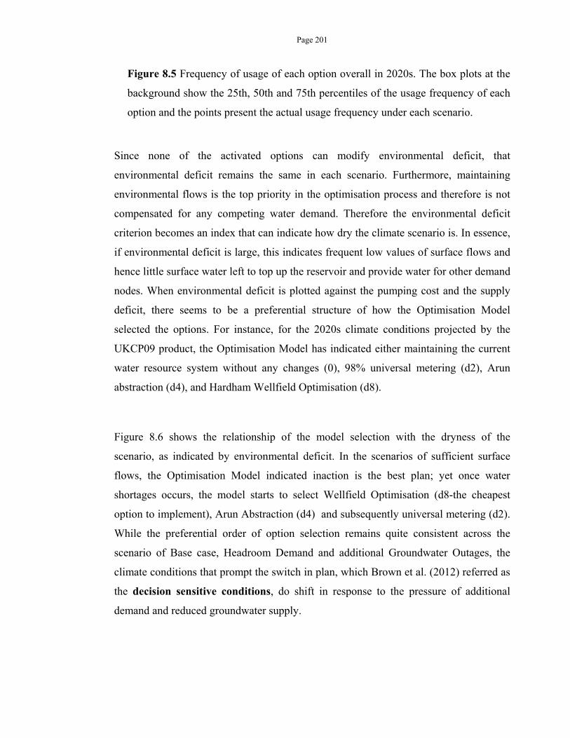
Page 201
Figure 8.5 Frequency of usage of each option overall in 2020s. The box plots at the
background show the 25th, 50th and 75th percentiles of the usage frequency of each
option and the points present the actual usage frequency under each scenario.
Since none of the activated options can modify environmental deficit, that
environmental deficit remains the same in each scenario. Furthermore, maintaining
environmental flows is the top priority in the optimisation process and therefore is not
compensated for any competing water demand. Therefore the environmental deficit
criterion becomes an index that can indicate how dry the climate scenario is. In essence,
if environmental deficit is large, this indicates frequent low values of surface flows and
hence little surface water left to top up the reservoir and provide water for other demand
nodes. When environmental deficit is plotted against the pumping cost and the supply
deficit, there seems to be a preferential structure of how the Optimisation Model
selected the options. For instance, for the 2020s climate conditions projected by the
UKCP09 product, the Optimisation Model has indicated either maintaining the current
water resource system without any changes (0), 98% universal metering (d2), Arun
abstraction (d4), and Hardham Wellfield Optimisation (d8).
Figure 8.6 shows the relationship of the model selection with the dryness of the
scenario, as indicated by environmental deficit. In the scenarios of sufficient surface
flows, the Optimisation Model indicated inaction is the best plan; yet once water
shortages occurs, the model starts to select Wellfield Optimisation (d8-the cheapest
option to implement), Arun Abstraction (d4) and subsequently universal metering (d2).
While the preferential order of option selection remains quite consistent across the
scenario of Base case, Headroom Demand and additional Groundwater Outages, the
climate conditions that prompt the switch in plan, which Brown et al. (2012) referred as
the decision sensitive conditions, do shift in response to the pressure of additional
demand and reduced groundwater supply.
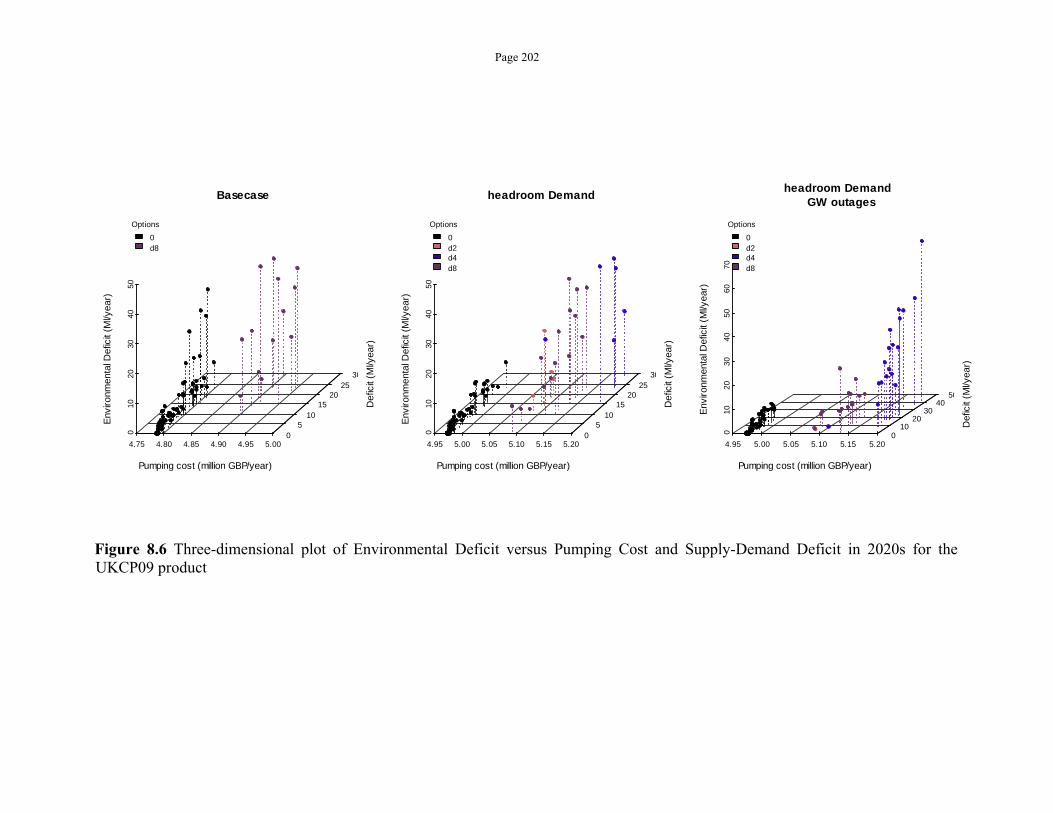
Page 202
Figure 8.6 Three-dimensional plot of Environmental Deficit versus Pumping Cost and Supply-Demand Deficit in 2020s for the UKCP09 product
Basecase
4.75 4.80 4.85 4.90 4.95 5.00
010
20
3040
50
0 5
1015
2025
30
Pumping cost (million GBP/year)
Def
icit
(Ml/y
ear)
Env
ironm
enta
l Def
icit
(Ml/y
ear)
Options
0d8
headroom Demand
4.95 5.00 5.05 5.10 5.15 5.20
010
20
3040
50
0 5
1015
2025
30
Pumping cost (million GBP/year)
Def
icit
(Ml/y
ear)
Env
ironm
enta
l Def
icit
(Ml/y
ear)
Options
0d2d4d8
headroom Demand GW outages
4.95 5.00 5.05 5.10 5.15 5.20
010
2030
4050
6070
010
2030
4050
Pumping cost (million GBP/year)
Def
icit
(Ml/y
ear)
Env
ironm
enta
l Def
icit
(Ml/y
ear)
Options
0d2d4d8
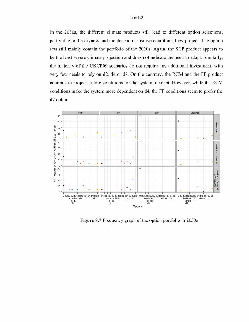
Page 203
In the 2030s, the different climate products still lead to different option selections,
partly due to the dryness and the decision sensitive conditions they project. The option
sets still mainly contain the portfolio of the 2020s. Again, the SCP product appears to
be the least severe climate projection and does not indicate the need to adapt. Similarly,
the majority of the UKCP09 scenarios do not require any additional investment, with
very few needs to rely on d2, d4 or d8. On the contrary, the RCM and the FF product
continue to project testing conditions for the system to adapt. However, while the RCM
conditions make the system more dependent on d4, the FF conditions seem to prefer the
d7 option.
Figure 8.7 Frequency graph of the option portfolio in 2030s
RCM FF SCP UKCP09
0
25
50
75
100
0
25
50
75
100
0
25
50
75
100
Basecase
headroom D
emand
headroom D
emand
GW
outages
0 d2d2d4
d2d4d7d8
d2d4d8
d2d7
d2d8
d4 d4d7
d4d8
d7d7d8
d8 0 d2d2d4
d2d4d7d8
d2d4d8
d2d7
d2d8
d4d4d7
d4d8
d7d7d8
d8 0 d2d2d4
d2d4d7d8
d2d4d8
d2d7
d2d8
d4 d4d7
d4d8
d7d7d8
d8 0 d2 d2d4
d2d4d7d8
d2d4d8
d2d7
d2d8
d4d4d7
d4d8
d7d7d8
d8
Options
% F
req
uen
cy S
ele
ctio
n w
ithin
all
Sce
nar
ios
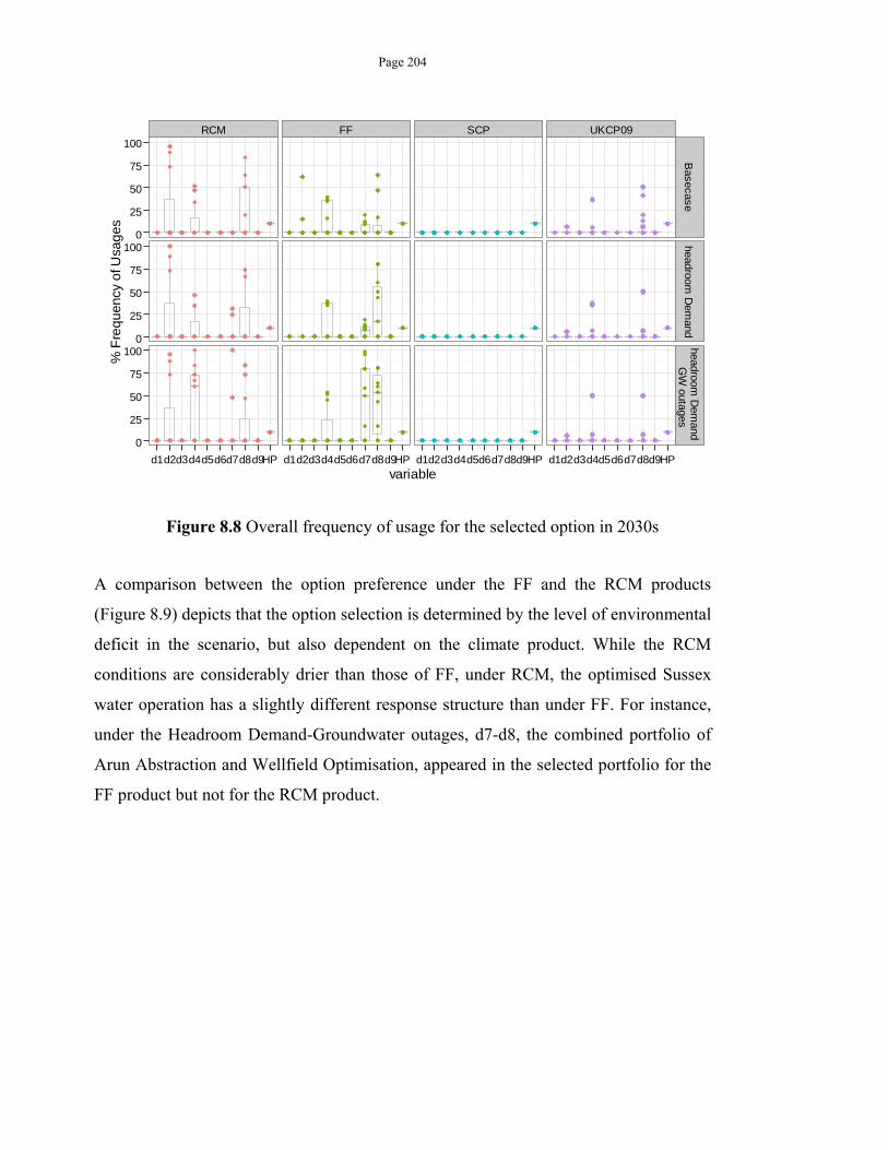
Page 204
Figure 8.8 Overall frequency of usage for the selected option in 2030s
A comparison between the option preference under the FF and the RCM products
(Figure 8.9) depicts that the option selection is determined by the level of environmental
deficit in the scenario, but also dependent on the climate product. While the RCM
conditions are considerably drier than those of FF, under RCM, the optimised Sussex
water operation has a slightly different response structure than under FF. For instance,
under the Headroom Demand-Groundwater outages, d7-d8, the combined portfolio of
Arun Abstraction and Wellfield Optimisation, appeared in the selected portfolio for the
FF product but not for the RCM product.
RCM FF SCP UKCP09
0
25
50
75
100
0
25
50
75
100
0
25
50
75
100
Basecase
headroom D
emand
headroom D
emand
GW
outages
d1d2d3d4d5d6d7d8d9HP d1d2d3d4d5d6d7d8d9HP d1d2d3d4d5d6d7d8d9HP d1d2d3d4d5d6d7d8d9HPvariable
% F
req
uency
of U
sag
es
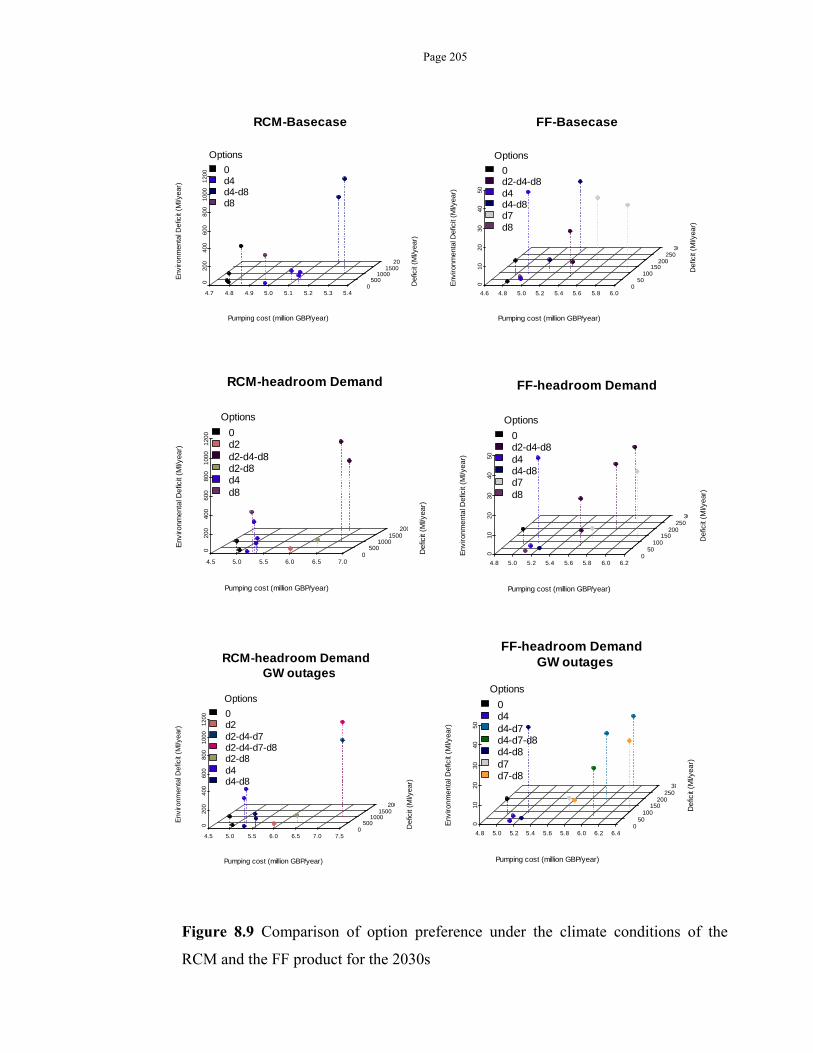
Page 205
Figure 8.9 Comparison of option preference under the climate conditions of the
RCM and the FF product for the 2030s
RCM-Basecase
4.7 4.8 4.9 5.0 5.1 5.2 5.3 5.4
0
200
400
600
800
1000
1200
0 500
10001500
20
Pumping cost (million GBP/year)
Def
icit
(Ml/y
ear)
Env
ironm
enta
l Def
icit
(Ml/y
ear)
Options
0d4d4-d8d8
FF-Basecase
4.6 4.8 5.0 5.2 5.4 5.6 5.8 6.0
010
2030
4050
0 50
100150
200250
30
Pumping cost (million GBP/year)
Def
icit
(Ml/y
ear)
Env
ironm
enta
l Def
icit
(Ml/y
ear)
Options
0d2-d4-d8d4d4-d8d7d8
RCM-headroom Demand
4.5 5.0 5.5 6.0 6.5 7.0
0
200
400
600
800
1000
1200
0 500
10001500
200
Pumping cost (million GBP/year)
Def
icit
(Ml/y
ear)
Env
ironm
enta
l Def
icit
(Ml/y
ear)
Options
0d2d2-d4-d8d2-d8d4d8
FF-headroom Demand
4.8 5.0 5.2 5.4 5.6 5.8 6.0 6.2
010
20
30
4050
0 50
100150
200250
30
Pumping cost (million GBP/year)
Def
icit
(Ml/y
ear)
Env
ironm
enta
l Def
icit
(Ml/y
ear)
Options
0d2-d4-d8d4d4-d8d7d8
RCM-headroom Demand GW outages
4.5 5.0 5.5 6.0 6.5 7.0 7.5
0
200
400
600
800
1000
1200
0 500
10001500
200
Pumping cost (million GBP/year)
Def
icit
(Ml/y
ear)
Env
ironm
enta
l Def
icit
(Ml/y
ear)
Options
0d2d2-d4-d7d2-d4-d7-d8d2-d8d4d4-d8
FF-headroom Demand GW outages
4.8 5.0 5.2 5.4 5.6 5.8 6.0 6.2 6.4
010
2030
4050
0 50
100150
200250
30
Pumping cost (million GBP/year)
Def
icit
(Ml/y
ear)
Env
ironm
enta
l Def
icit
(Ml/y
ear)
Options
0d4d4-d7d4-d7-d8d4-d8d7d7-d8
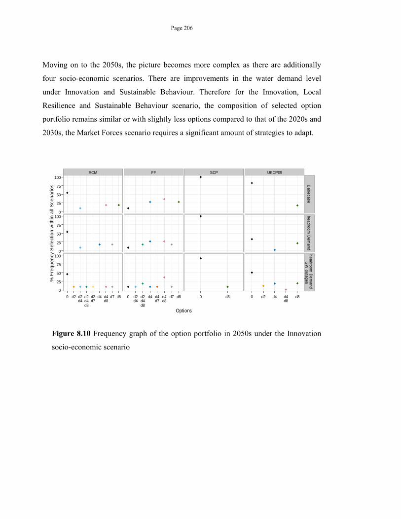
Page 206
Moving on to the 2050s, the picture becomes more complex as there are additionally
four socio-economic scenarios. There are improvements in the water demand level
under Innovation and Sustainable Behaviour. Therefore for the Innovation, Local
Resilience and Sustainable Behaviour scenario, the composition of selected option
portfolio remains similar or with slightly less options compared to that of the 2020s and
2030s, the Market Forces scenario requires a significant amount of strategies to adapt.
Figure 8.10 Frequency graph of the option portfolio in 2050s under the Innovation
socio-economic scenario
RCM FF SCP UKCP09
0
25
50
75
100
0
25
50
75
100
0
25
50
75
100
Basecase
headroom D
emand
headroom D
emand
GW
outages
0 d2 d2d4
d2d4d8
d2d7
d4 d4d8
d7 d8 0 d2d4
d2d4d8
d4 d4d7
d4d8
d7 d8 0 d8 0 d2 d4 d4d8
d8
Options
% F
req
ue
ncy
Se
lect
ion
with
in a
ll S
cen
ari
os
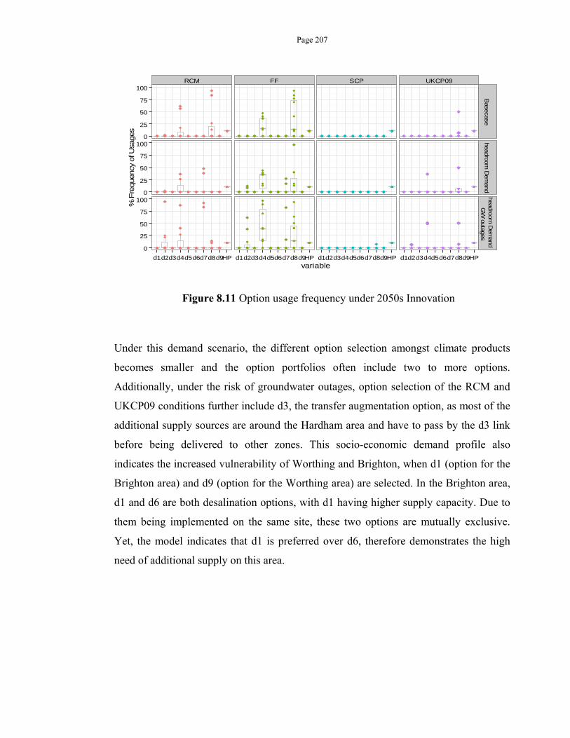
Page 207
Figure 8.11 Option usage frequency under 2050s Innovation
Under this demand scenario, the different option selection amongst climate products
becomes smaller and the option portfolios often include two to more options.
Additionally, under the risk of groundwater outages, option selection of the RCM and
UKCP09 conditions further include d3, the transfer augmentation option, as most of the
additional supply sources are around the Hardham area and have to pass by the d3 link
before being delivered to other zones. This socio-economic demand profile also
indicates the increased vulnerability of Worthing and Brighton, when d1 (option for the
Brighton area) and d9 (option for the Worthing area) are selected. In the Brighton area,
d1 and d6 are both desalination options, with d1 having higher supply capacity. Due to
them being implemented on the same site, these two options are mutually exclusive.
Yet, the model indicates that d1 is preferred over d6, therefore demonstrates the high
need of additional supply on this area.
RCM FF SCP UKCP09
0
25
50
75
100
0
25
50
75
100
0
25
50
75
100
Basecase
headroom D
emand
headroom D
emand
GW
outages
d1d2d3d4d5d6d7d8d9HP d1d2d3d4d5d6d7d8d9HP d1d2d3d4d5d6d7d8d9HP d1d2d3d4d5d6d7d8d9HPvariable
% F
requ
ency
of U
sage
s
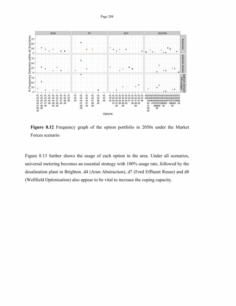
Page 208
Figure 8.12 Frequency graph of the option portfolio in 2050s under the Market
Forces scenario
Figure 8.13 further shows the usage of each option in the area. Under all scenarios,
universal metering becomes an essential strategy with 100% usage rate, followed by the
desalination plant in Brighton. d4 (Arun Abstraction), d7 (Ford Effluent Reuse) and d8
(Wellfield Optimisation) also appear to be vital to increase the coping capacity.
RCM FF SCP UKCP09
0
25
50
75
0
25
50
75
0
25
50
75
Basecase
headroom D
emand
eadroom D
emand
GW
outages
d1d2d3d4d7d8d9
d1d2d4d7d8d9
d1d2d4d7d9
d1d2d4d8
d1d2d4d8d9
d1d2d7d8d9
d1d2d7d9
d1d2d8d9
d1d2d9
d1d2d4
d1d2d4d7d8d9
d1d2d4d7d9
d1d2d7d8d9
d1d2d8d9
d1d2d9
d1d2d4
d1d2d4d7
d1d2d4d7d9
d1d2d4d8
d1d2d4d8d9
d1d2d4d9
d1d2d7
d1d2d7d8
d1d2d7d8d9
d1d2d7d9
d1d2d8
d1d2
d1d2d3d4d7d8d9
d1d2d4
d1d2d4d7
d1d2d4d7d8
d1d2d4d7d8d9
d1d2d4d7d9
d1d2d4d8
d1d2d4d8d9
d1d2d4d9
d1d2d7
d1d2d7d8
d1d2d7d8d9
d1d2d7d9
d1d2d8
d1d2d8d9
Options
% F
req
ue
ncy
Se
lect
ion
with
in a
ll S
cen
ari
os
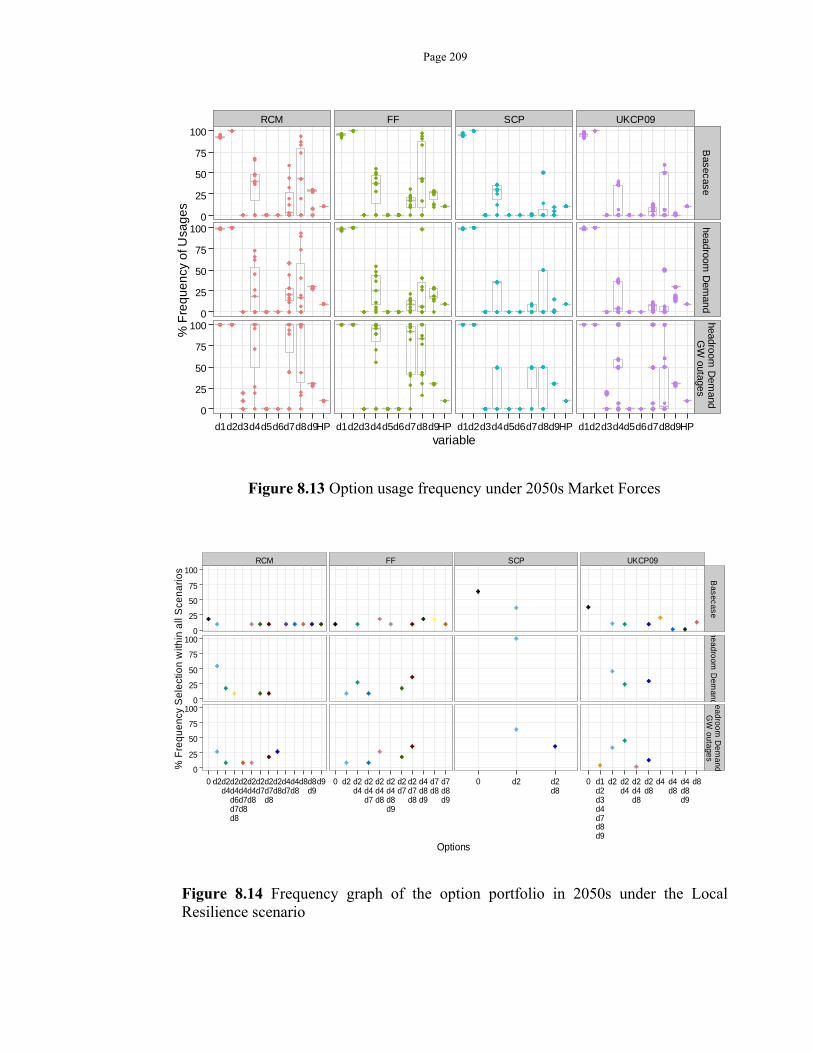
Page 209
Figure 8.13 Option usage frequency under 2050s Market Forces
Figure 8.14 Frequency graph of the option portfolio in 2050s under the Local Resilience scenario
RCM FF SCP UKCP09
0
25
50
75
100
0
25
50
75
100
0
25
50
75
100
Basecase
headroom D
emand
headroom D
emand
GW
outages
d1d2d3d4d5d6d7d8d9HP d1d2d3d4d5d6d7d8d9HP d1d2d3d4d5d6d7d8d9HP d1d2d3d4d5d6d7d8d9HPvariable
% F
req
uen
cy o
f Usa
ge
s
RCM FF SCP UKCP09
0
25
50
75
100
0
25
50
75
100
0
25
50
75
100
Basecase
headroom D
emand
eadroom D
emand
GW
outages
0 d2d2d4
d2d4d6d7d8
d2d4d7d8
d2d4d8
d2d7
d2d7d8
d2d8
d4d7
d4d8
d8d8d9
d9 0 d2 d2d4
d2d4d7
d2d4d8
d2d4d8d9
d2d7
d2d7d8
d4d8d9
d7d8
d7d8d9
0 d2 d2d8
0 d1d2d3d4d7d8d9
d2 d2d4
d2d4d8
d2d8
d4 d4d8
d4d8d9
d8
Options
% F
req
uen
cy S
ele
ctio
n w
ithin
all
Sce
nari
os
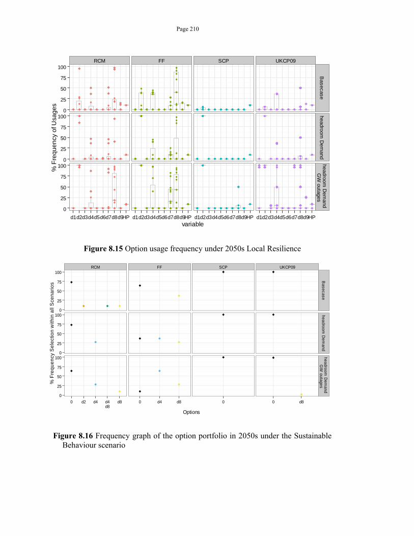
Page 210
Figure 8.15 Option usage frequency under 2050s Local Resilience
Figure 8.16 Frequency graph of the option portfolio in 2050s under the Sustainable Behaviour scenario
RCM FF SCP UKCP09
0
25
50
75
100
0
25
50
75
100
0
25
50
75
100
Basecase
headroom D
emand
headroom D
emand
GW
outages
d1d2d3d4d5d6d7d8d9HP d1d2d3d4d5d6d7d8d9HP d1d2d3d4d5d6d7d8d9HP d1d2d3d4d5d6d7d8d9HPvariable
% F
req
ue
ncy
of U
sag
es
RCM FF SCP UKCP09
0
25
50
75
100
0
25
50
75
100
0
25
50
75
100
Basecase
headroom D
emand
headroom D
emand
GW
outages
0 d2 d4 d4d8
d8 0 d4 d8 0 0 d8
Options
% F
req
ue
ncy
Se
lect
ion
with
in a
ll S
cen
ari
os
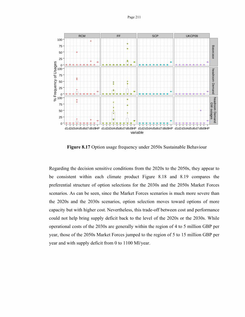
Page 211
Figure 8.17 Option usage frequency under 2050s Sustainable Behaviour
Regarding the decision sensitive conditions from the 2020s to the 2050s, they appear to
be consistent within each climate product Figure 8.18 and 8.19 compares the
preferential structure of option selections for the 2030s and the 2050s Market Forces
scenarios. As can be seen, since the Market Forces scenarios is much more severe than
the 2020s and the 2030s scenarios, option selection moves toward options of more
capacity but with higher cost. Nevertheless, this trade-off between cost and performance
could not help bring supply deficit back to the level of the 2020s or the 2030s. While
operational costs of the 2030s are generally within the region of 4 to 5 million GBP per
year, those of the 2050s Market Forces jumped to the region of 5 to 15 million GBP per
year and with supply deficit from 0 to 1100 Ml/year.
RCM FF SCP UKCP09
0
25
50
75
100
0
25
50
75
100
0
25
50
75
100
Basecase
headroom D
emand
headroom D
emand
GW
outages
d1d2d3d4d5d6d7d8d9HP d1d2d3d4d5d6d7d8d9HP d1d2d3d4d5d6d7d8d9HP d1d2d3d4d5d6d7d8d9HPvariable
% F
req
ue
ncy
of U
sag
es
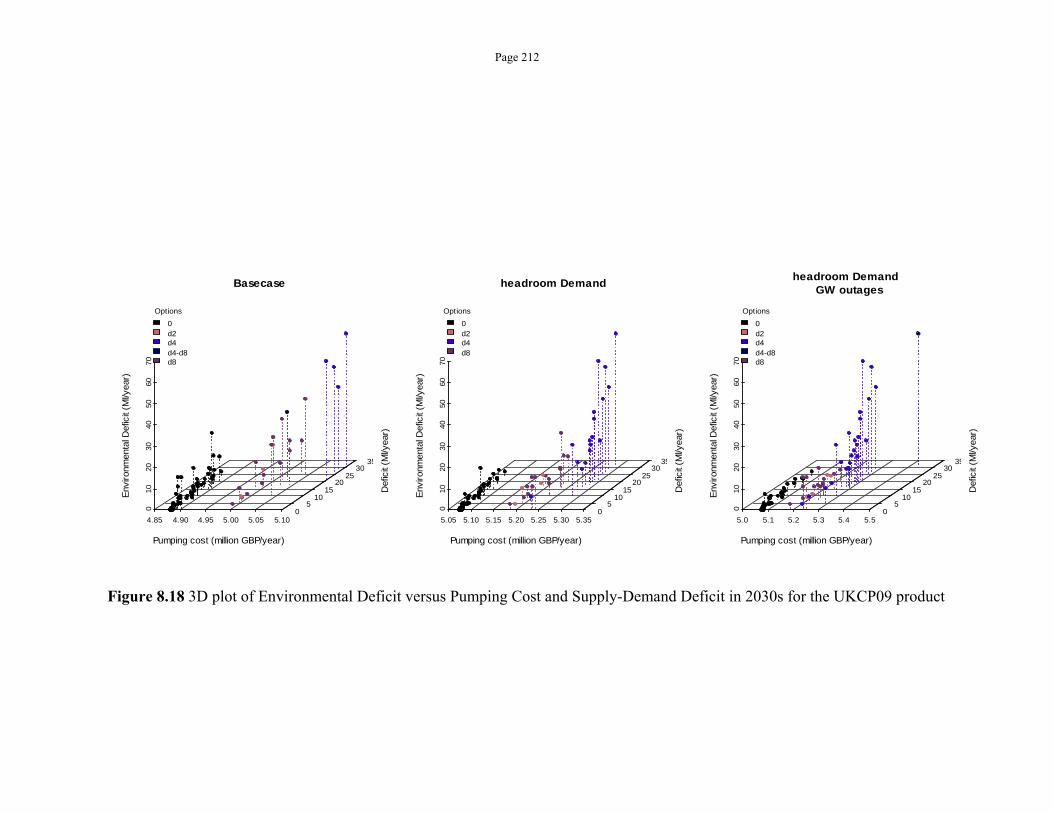
Page 212
Figure 8.18 3D plot of Environmental Deficit versus Pumping Cost and Supply-Demand Deficit in 2030s for the UKCP09 product
Basecase
4.85 4.90 4.95 5.00 5.05 5.10
010
2030
4050
6070
0 5
1015
2025
3035
Pumping cost (million GBP/year)
Def
icit
(Ml/y
ear)
Env
ironm
enta
l Def
icit
(Ml/y
ear)
Options
0d2d4d4-d8d8
headroom Demand
5.05 5.10 5.15 5.20 5.25 5.30 5.35
010
2030
4050
6070
0 5
1015
2025
3035
Pumping cost (million GBP/year)
Def
icit
(Ml/y
ear)
Env
ironm
enta
l Def
icit
(Ml/y
ear)
Options
0d2d4d8
headroom Demand GW outages
5.0 5.1 5.2 5.3 5.4 5.5
010
2030
4050
6070
0 5
1015
2025
3035
Pumping cost (million GBP/year)
Def
icit
(Ml/y
ear)
Env
ironm
enta
l Def
icit
(Ml/y
ear)
Options
0d2d4d4-d8d8
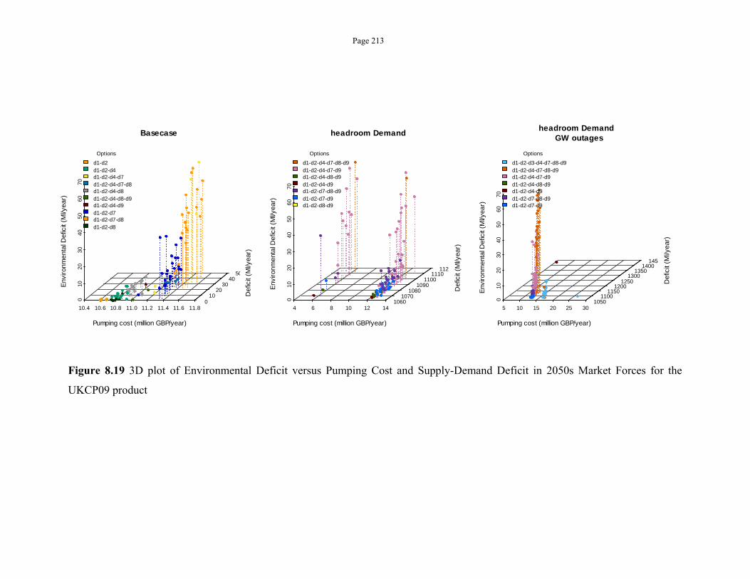
Page 213
Figure 8.19 3D plot of Environmental Deficit versus Pumping Cost and Supply-Demand Deficit in 2050s Market Forces for the
UKCP09 product
Basecase
10.4 10.6 10.8 11.0 11.2 11.4 11.6 11.8
010
20
3040
50
6070
010
2030
4050
Pumping cost (million GBP/year)
Def
icit
(Ml/y
ear)
Env
ironm
enta
l Def
icit
(Ml/y
ear)
Options
d1-d2d1-d2-d4d1-d2-d4-d7d1-d2-d4-d7-d8d1-d2-d4-d8d1-d2-d4-d8-d9d1-d2-d4-d9d1-d2-d7d1-d2-d7-d8d1-d2-d8
headroom Demand
4 6 8 10 12 14
01
020
3040
506
070
10601070
10801090
11001110
1120
Pumping cost (million GBP/year)
Def
icit
(Ml/y
ear)
Env
ironm
enta
l Def
icit
(Ml/y
ear)
Options
d1-d2-d4-d7-d8-d9d1-d2-d4-d7-d9d1-d2-d4-d8-d9d1-d2-d4-d9d1-d2-d7-d8-d9d1-d2-d7-d9d1-d2-d8-d9
headroom Demand GW outages
5 10 15 20 25 30
01
020
3040
50
6070
10501100
11501200
12501300
13501400
1450
Pumping cost (million GBP/year)
Def
icit
(Ml/y
ear)
Env
ironm
enta
l Def
icit
(Ml/y
ear)
Options
d1-d2-d3-d4-d7-d8-d9d1-d2-d4-d7-d8-d9d1-d2-d4-d7-d9d1-d2-d4-d8-d9d1-d2-d4-d9d1-d2-d7-d8-d9d1-d2-d7-d9
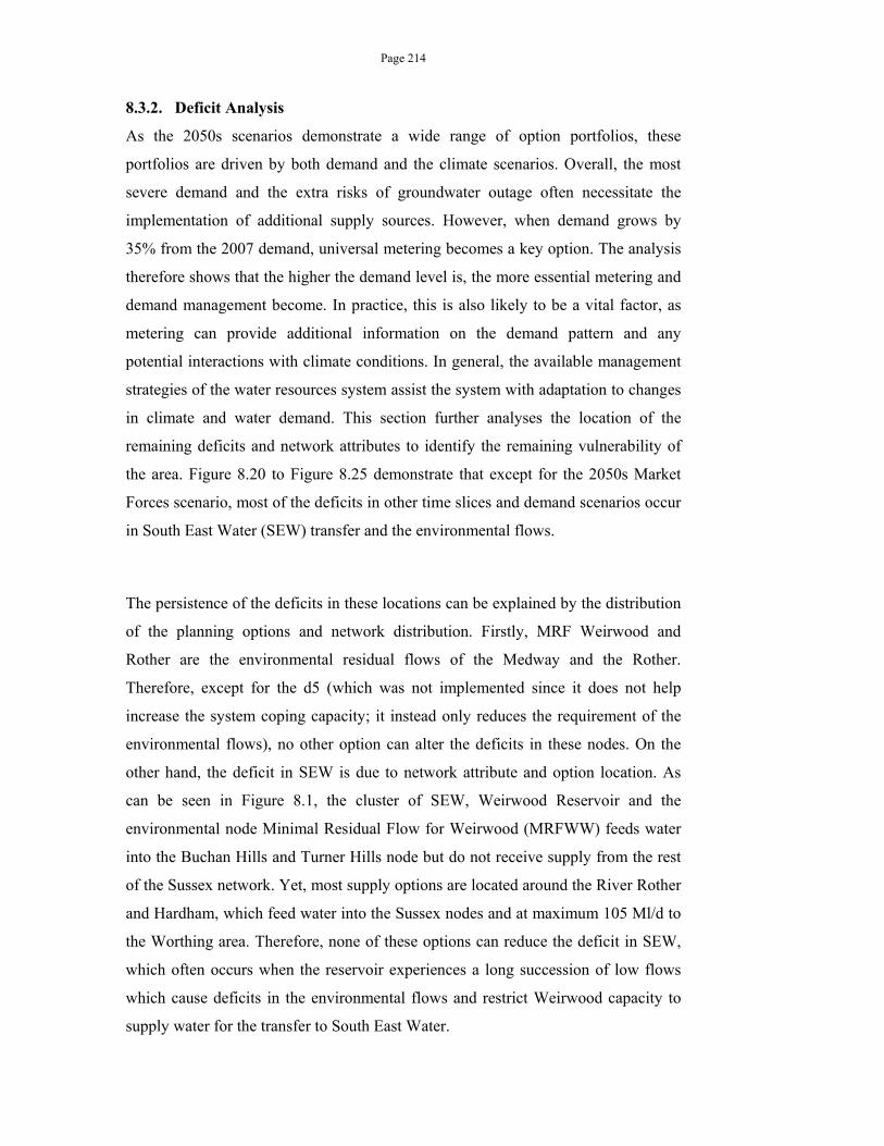
Page 214
8.3.2. Deficit Analysis
As the 2050s scenarios demonstrate a wide range of option portfolios, these
portfolios are driven by both demand and the climate scenarios. Overall, the most
severe demand and the extra risks of groundwater outage often necessitate the
implementation of additional supply sources. However, when demand grows by
35% from the 2007 demand, universal metering becomes a key option. The analysis
therefore shows that the higher the demand level is, the more essential metering and
demand management become. In practice, this is also likely to be a vital factor, as
metering can provide additional information on the demand pattern and any
potential interactions with climate conditions. In general, the available management
strategies of the water resources system assist the system with adaptation to changes
in climate and water demand. This section further analyses the location of the
remaining deficits and network attributes to identify the remaining vulnerability of
the area. Figure 8.20 to Figure 8.25 demonstrate that except for the 2050s Market
Forces scenario, most of the deficits in other time slices and demand scenarios occur
in South East Water (SEW) transfer and the environmental flows.
The persistence of the deficits in these locations can be explained by the distribution
of the planning options and network distribution. Firstly, MRF Weirwood and
Rother are the environmental residual flows of the Medway and the Rother.
Therefore, except for the d5 (which was not implemented since it does not help
increase the system coping capacity; it instead only reduces the requirement of the
environmental flows), no other option can alter the deficits in these nodes. On the
other hand, the deficit in SEW is due to network attribute and option location. As
can be seen in Figure 8.1, the cluster of SEW, Weirwood Reservoir and the
environmental node Minimal Residual Flow for Weirwood (MRFWW) feeds water
into the Buchan Hills and Turner Hills node but do not receive supply from the rest
of the Sussex network. Yet, most supply options are located around the River Rother
and Hardham, which feed water into the Sussex nodes and at maximum 105 Ml/d to
the Worthing area. Therefore, none of these options can reduce the deficit in SEW,
which often occurs when the reservoir experiences a long succession of low flows
which cause deficits in the environmental flows and restrict Weirwood capacity to
supply water for the transfer to South East Water.
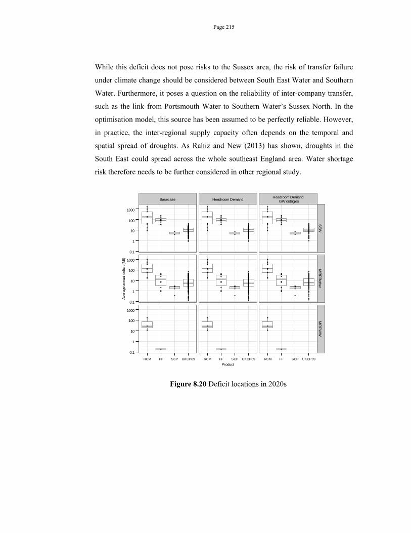
Page 215
While this deficit does not pose risks to the Sussex area, the risk of transfer failure
under climate change should be considered between South East Water and Southern
Water. Furthermore, it poses a question on the reliability of inter-company transfer,
such as the link from Portsmouth Water to Southern Water’s Sussex North. In the
optimisation model, this source has been assumed to be perfectly reliable. However,
in practice, the inter-regional supply capacity often depends on the temporal and
spatial spread of droughts. As Rahiz and New (2013) has shown, droughts in the
South East could spread across the whole southeast England area. Water shortage
risk therefore needs to be further considered in other regional study.
Figure 8.20 Deficit locations in 2020s
Basecase Headroom DemandHeadroom Demand
GW outages
0.1
1
10
100
1000
0.1
1
10
100
1000
0.1
1
10
100
1000
SE
WM
RF
Rother
MR
FW
W
RCM FF SCP UKCP09 RCM FF SCP UKCP09 RCM FF SCP UKCP09
Product
Ave
rage
ann
ual d
efic
it (M
l)
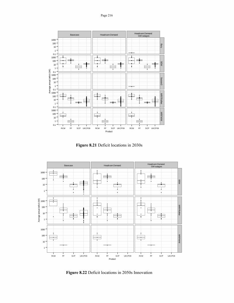
Page 216
Figure 8.21 Deficit locations in 2030s
Figure 8.22 Deficit locations in 2050s Innovation
Basecase Headroom DemandHeadroom Demand
GW outages
0.1
1
10
100
1000
0.1
1
10
100
1000
0.1
1
10
100
1000
0.1
1
10
100
1000
0.1
1
10
100
1000
Bury
SE
WS
ussex3M
RF
Rother
MR
FW
W
RCM FF SCP UKCP09 RCM FF SCP UKCP09 RCM FF SCP UKCP09
Product
Ave
rage
ann
ual d
efic
it (M
l)
Basecase Headroom DemandHeadroom Demand
GW outages
1
10
100
1000
1
10
100
1000
1
10
100
1000
SE
WM
RF
Rother
MR
FW
W
RCM FF SCP UKCP09 RCM FF SCP UKCP09 RCM FF SCP UKCP09
Product
Ave
rage
ann
ual d
efic
it (M
l)
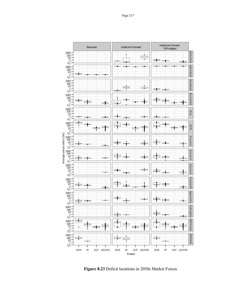
Page 217
Figure 8.23 Deficit locations in 2050s Market Forces
Basecase Headroom DemandHeadroom Demand
GW outages
0.11
10100
1000
0.11
10100
1000
0.11
10100
1000
0.11
10100
1000
0.11
10100
1000
0.11
10100
1000
0.11
10100
1000
0.11
10100
1000
0.11
10100
1000
0.11
10100
1000
0.11
10100
1000
0.11
10100
1000
0.11
10100
1000
0.11
10100
1000
righ
ton
De
mrig
hto
nD
em
Sh
ore
ha
mB
uc
ha
nH
illB
ury
SE
WS
us
se
x2
Su
ss
ex
3S
us
se
x4
Tu
rne
rsH
illU
pp
erV
alle
yWo
rthin
gD
em
MR
FR
oth
er
MR
FW
W
RCM FF SCP UKCP09 RCM FF SCP UKCP09 RCM FF SCP UKCP09
Product
Ave
rage
ann
ual d
efic
it (M
l)
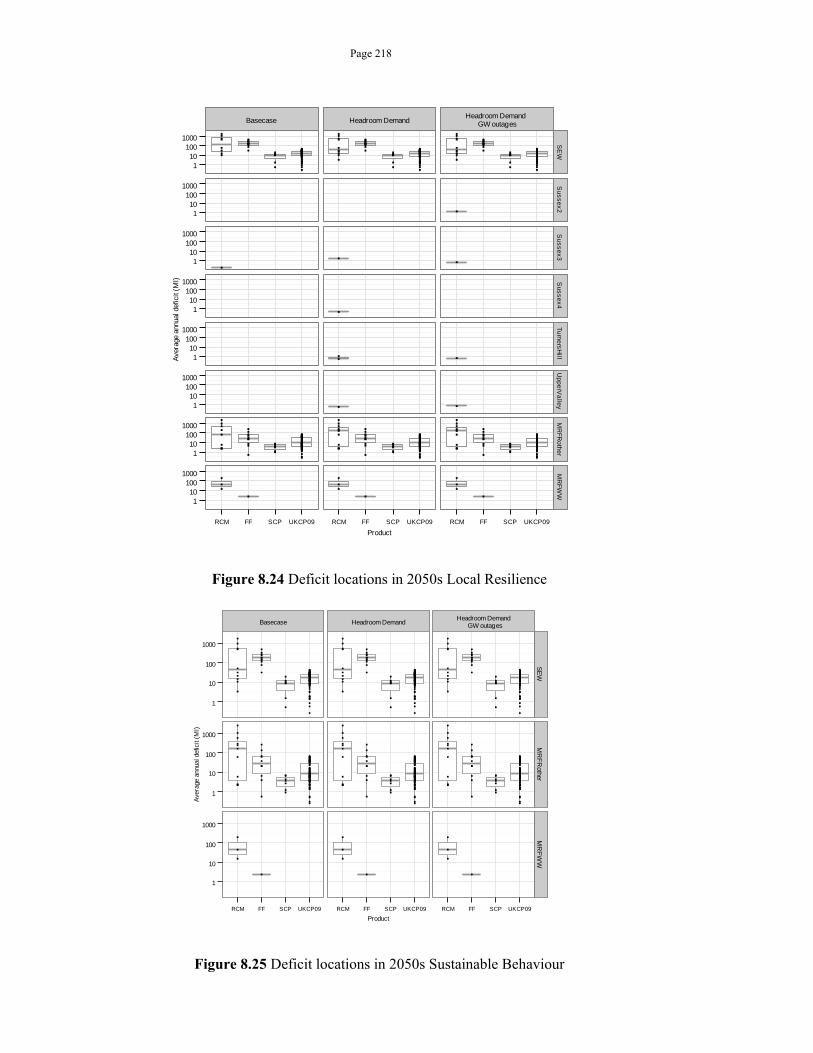
Page 218
Figure 8.24 Deficit locations in 2050s Local Resilience
Figure 8.25 Deficit locations in 2050s Sustainable Behaviour
Basecase Headroom DemandHeadroom Demand
GW outages
110
1001000
110
1001000
110
1001000
110
1001000
110
1001000
110
1001000
110
1001000
110
1001000
SE
WS
us
se
x2
Su
ss
ex
3S
us
se
x4
Tu
rne
rsH
illU
pp
erV
alle
yM
RF
Ro
the
rM
RF
WW
RCM FF SCP UKCP09 RCM FF SCP UKCP09 RCM FF SCP UKCP09
Product
Ave
rage
ann
ual d
efic
it (M
l)
Basecase Headroom DemandHeadroom Demand
GW outages
1
10
100
1000
1
10
100
1000
1
10
100
1000
SE
WM
RF
Rother
MR
FW
W
RCM FF SCP UKCP09 RCM FF SCP UKCP09 RCM FF SCP UKCP09
Product
Ave
rage
ann
ual d
efic
it (M
l)
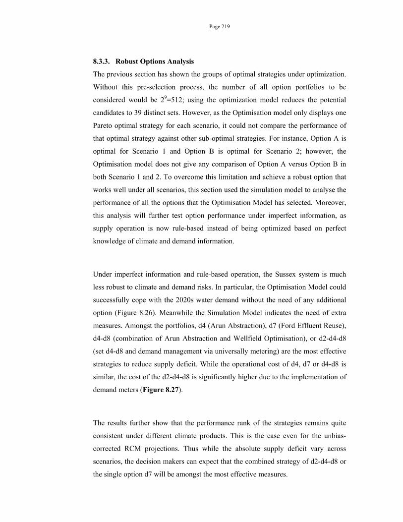
Page 219
8.3.3. Robust Options Analysis
The previous section has shown the groups of optimal strategies under optimization.
Without this pre-selection process, the number of all option portfolios to be
considered would be 29=512; using the optimization model reduces the potential
candidates to 39 distinct sets. However, as the Optimisation model only displays one
Pareto optimal strategy for each scenario, it could not compare the performance of
that optimal strategy against other sub-optimal strategies. For instance, Option A is
optimal for Scenario 1 and Option B is optimal for Scenario 2; however, the
Optimisation model does not give any comparison of Option A versus Option B in
both Scenario 1 and 2. To overcome this limitation and achieve a robust option that
works well under all scenarios, this section used the simulation model to analyse the
performance of all the options that the Optimisation Model has selected. Moreover,
this analysis will further test option performance under imperfect information, as
supply operation is now rule-based instead of being optimized based on perfect
knowledge of climate and demand information.
Under imperfect information and rule-based operation, the Sussex system is much
less robust to climate and demand risks. In particular, the Optimisation Model could
successfully cope with the 2020s water demand without the need of any additional
option (Figure 8.26). Meanwhile the Simulation Model indicates the need of extra
measures. Amongst the portfolios, d4 (Arun Abstraction), d7 (Ford Effluent Reuse),
d4-d8 (combination of Arun Abstraction and Wellfield Optimisation), or d2-d4-d8
(set d4-d8 and demand management via universally metering) are the most effective
strategies to reduce supply deficit. While the operational cost of d4, d7 or d4-d8 is
similar, the cost of the d2-d4-d8 is significantly higher due to the implementation of
demand meters (Figure 8.27).
The results further show that the performance rank of the strategies remains quite
consistent under different climate products. This is the case even for the unbias-
corrected RCM projections. Thus while the absolute supply deficit vary across
scenarios, the decision makers can expect that the combined strategy of d2-d4-d8 or
the single option d7 will be amongst the most effective measures.
Page 220
Figure 8.26 Average annual supply deficit in the 2020s. The % Frequency colour
gradient shows how often the option was selected in the Optimisation Model,
such that the option in red was the dominant option of the Optimisation Model.
Figure 8.27 Average annual supply cost in the 2020s. The % Frequency colour
gradient shows how often the option was selected in the Optimisation Model,
such that the option in red was the dominant option of the Optimisation Model.
Basecase headroom Demand headroom Demand GW outages
0
500
1000
0
100
200
300
0
10
20
0
25
50
75
100
RC
MF
FS
CP
UK
CP
09
0 d4 d7 d8 d4d8
d2d4d8
0 d4 d7 d8 d4d8
d2d4d8
0 d4 d7 d8 d4d8
d2d4d8
Option
20
20
Ave
rag
e A
nn
ua
l De
ficit
(Ml)
0
25
50
75
100Frequency
Basecase headroom Demand headroom Demand GW outages
1.5
2.0
2.5
3.0
3.5
1.5
2.0
2.5
3.0
3.5
1.5
2.0
2.5
3.0
3.5
1.5
2.0
2.5
3.0
3.5
RC
MF
FS
CP
UK
CP
09
0 d4 d7 d8 d4d8
d2d4d8
0 d4 d7 d8 d4d8
d2d4d8
0 d4 d7 d8 d4d8
d2d4d8
Option
205
0 A
vera
ge
an
nua
l sup
ply
and
ope
ratio
na
l cos
t (m
illio
n G
BP
)
0
25
50
75
100Frequency

Page 221
In other words, the post-processing uncertainty in climate projections is a significant
uncertainty factor in determining the climate change impacts; however, in terms of
decision making, this uncertainty do not play a major role and the preferential
ranking of the options is still preserved. While both have similar mean effect, effect
variation (represented by the span of the box plot) of the former is smaller than that
of the latter; yet, d2-d4-d8 is significantly more expensive to implement and operate
than d7.
Overall, the Simulation Model indicates that all the measures could restrict supply
deficit to under 150 Ml/year; however the particular selection will be dependent on
the financial budget and the risk averseness level of the decision maker. The results
also highlight the impacts of scenario variation to option selection. Under the time
series-based RCM and FF products, the selected optimal options vary in response to
the decision sensitive conditions and the dryness of the scenario. Meanwhile, the
Change Factor-based SCP and UKCP09 have a strong dominant option for 2020s
and 2030s. However, the dominance of the inaction strategy (0) under the SCP and
UKCP09 product could also be due to their relatively less severe climate conditions,
compared to the RCM and FF products.
Considering the 2030s, the situation and the options remain similar to those of the
2020s. d7 and the portfolio d2-d4-d8 are still the best performing and least varying
strategies (Figure 8.28). Again, the adaptation choice depends on the decision
maker’s preference on the operational and investment cost, as well as the supply
safety margin of the option. However, the need to adapt is not yet pressing, and in
various scenarios, the system can still supply sufficiently deficit using the existing
sources.
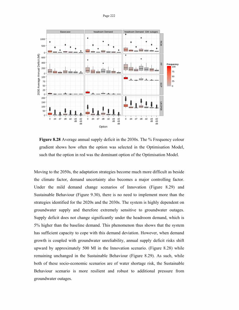
Page 222
Figure 8.28 Average annual supply deficit in the 2030s. The % Frequency colour
gradient shows how often the option was selected in the Optimisation Model,
such that the option in red was the dominant option of the Optimisation Model.
Moving to the 2050s, the adaptation strategies become much more difficult as beside
the climate factor, demand uncertainty also becomes a major controlling factor.
Under the mild demand change scenarios of Innovation (Figure 8.29) and
Sustainable Behaviour (Figure 9.30), there is no need to implement more than the
strategies identified for the 2020s and the 2030s. The system is highly dependent on
groundwater supply and therefore extremely sensitive to groundwater outages.
Supply deficit does not change significantly under the headroom demand, which is
5% higher than the baseline demand. This phenomenon thus shows that the system
has sufficient capacity to cope with this demand deviation. However, when demand
growth is coupled with groundwater unreliability, annual supply deficit risks shift
upward by approximately 500 Ml in the Innovation scenario. (Figure 8.28) while
remaining unchanged in the Sustainable Behaviour (Figure 8.29). As such, while
both of these socio-economic scenarios are of water shortage risk, the Sustainable
Behaviour scenario is more resilient and robust to additional pressure from
groundwater outages.
Basecase headroom Demand headroom Demand GW outages
0
500
1000
0
200
400
600
0
25
50
75
100
0
50
100
150
200
RC
MF
FS
CP
UK
CP
09
0 d4 d7 d8 d2 d4d8
d2d4d8
0 d4 d7 d8 d2 d4d8
d2d4d8
0 d4 d7 d8 d2 d4d8
d2d4d8
Option
203
0 A
vera
ge
An
nual
De
ficit
(Ml)
0
25
50
75
100Frequency
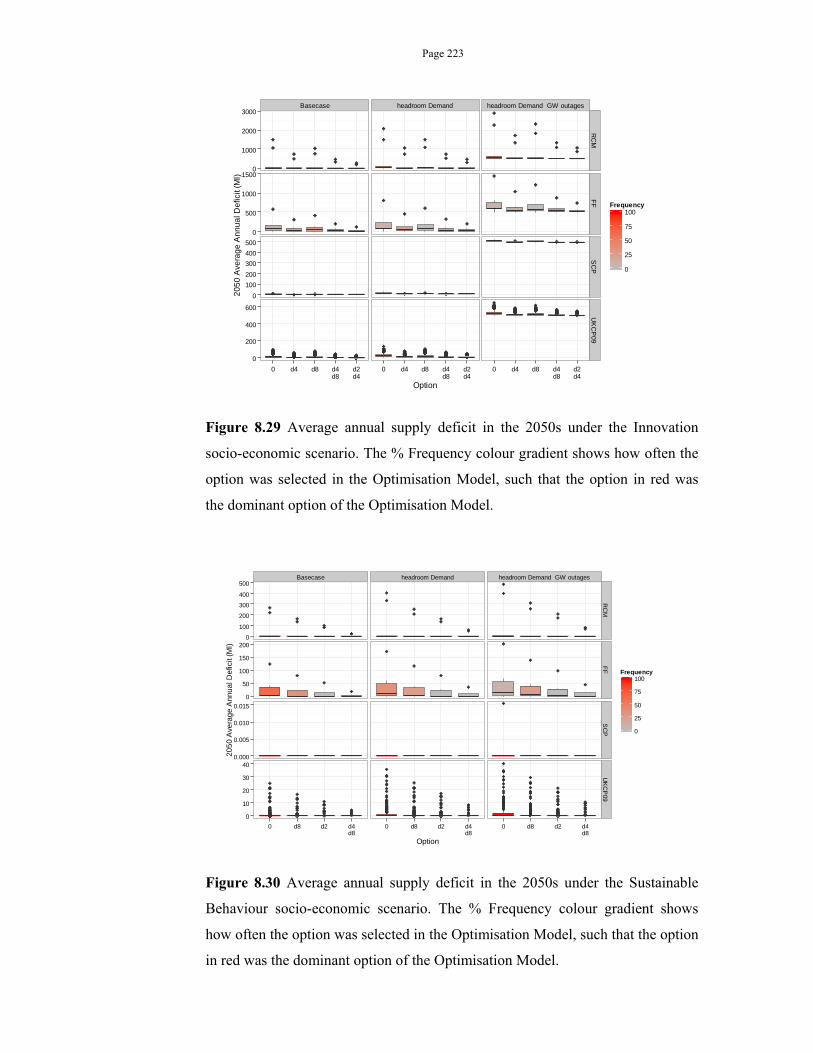
Page 223
Figure 8.29 Average annual supply deficit in the 2050s under the Innovation
socio-economic scenario. The % Frequency colour gradient shows how often the
option was selected in the Optimisation Model, such that the option in red was
the dominant option of the Optimisation Model.
Figure 8.30 Average annual supply deficit in the 2050s under the Sustainable
Behaviour socio-economic scenario. The % Frequency colour gradient shows
how often the option was selected in the Optimisation Model, such that the option
in red was the dominant option of the Optimisation Model.
Basecase headroom Demand headroom Demand GW outages
0
1000
2000
3000
0
500
1000
1500
0
100
200
300
400
500
0
200
400
600
RC
MF
FS
CP
UK
CP
09
0 d4 d8 d4d8
d2d4
0 d4 d8 d4d8
d2d4
0 d4 d8 d4d8
d2d4
Option
205
0 A
vera
ge
An
nua
l Def
icit
(Ml)
0
25
50
75
100Frequency
Basecase headroom Demand headroom Demand GW outages
0
100
200
300
400
500
0
50
100
150
200
0.000
0.005
0.010
0.015
0
10
20
30
40
RC
MF
FS
CP
UK
CP
09
0 d8 d2 d4d8
0 d8 d2 d4d8
0 d8 d2 d4d8
Option
20
50
Ave
rag
e A
nn
ua
l De
ficit
(Ml)
0
25
50
75
100Frequency
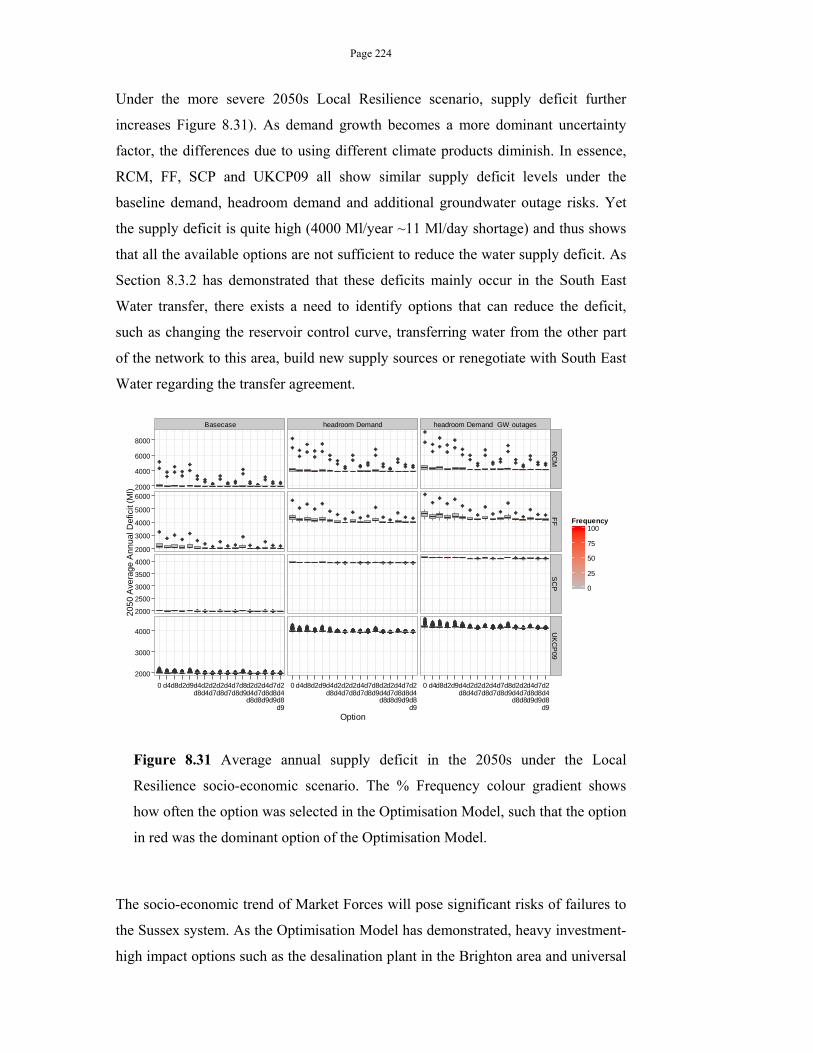
Page 224
Under the more severe 2050s Local Resilience scenario, supply deficit further
increases Figure 8.31). As demand growth becomes a more dominant uncertainty
factor, the differences due to using different climate products diminish. In essence,
RCM, FF, SCP and UKCP09 all show similar supply deficit levels under the
baseline demand, headroom demand and additional groundwater outage risks. Yet
the supply deficit is quite high (4000 Ml/year ~11 Ml/day shortage) and thus shows
that all the available options are not sufficient to reduce the water supply deficit. As
Section 8.3.2 has demonstrated that these deficits mainly occur in the South East
Water transfer, there exists a need to identify options that can reduce the deficit,
such as changing the reservoir control curve, transferring water from the other part
of the network to this area, build new supply sources or renegotiate with South East
Water regarding the transfer agreement.
Figure 8.31 Average annual supply deficit in the 2050s under the Local
Resilience socio-economic scenario. The % Frequency colour gradient shows
how often the option was selected in the Optimisation Model, such that the option
in red was the dominant option of the Optimisation Model.
The socio-economic trend of Market Forces will pose significant risks of failures to
the Sussex system. As the Optimisation Model has demonstrated, heavy investment-
high impact options such as the desalination plant in the Brighton area and universal
Basecase headroom Demand headroom Demand GW outages
2000
4000
6000
8000
2000
3000
4000
5000
6000
2000
2500
3000
3500
4000
2000
3000
4000
RC
MF
FS
CP
UK
CP
09
0 d4d8d2d9d4d8
d2d4
d2d7
d2d8
d4d7
d7d8
d8d9
d2d4d8
d2d7d8
d4d8d9
d7d8d9
d2d4d8d9
0 d4d8d2d9d4d8
d2d4
d2d7
d2d8
d4d7
d7d8
d8d9
d2d4d8
d2d7d8
d4d8d9
d7d8d9
d2d4d8d9
0 d4d8d2d9d4d8
d2d4
d2d7
d2d8
d4d7
d7d8
d8d9
d2d4d8
d2d7d8
d4d8d9
d7d8d9
d2d4d8d9
Option
20
50
Ave
rag
e A
nn
ua
l De
ficit
(Ml)
0
25
50
75
100Frequency
Page 225
metering in the whole area become necessary. Under the 2050 Market Forces
scenarios, the single options are not adequate to abate supply shortages;
consequently all the selected sets contain at least two options (Figure 8.32). While
offering more coping capacity to drought risks, the combined options are often
expensive and the operation cost of the system increases with the addition of each
option (Figure 8.33). Under a 5% increase from the baseline demand, the overall
supply deficit increases; however when groundwater supply reduces, the system
suffers less deficit shortages overall; however analysis on each water resource area
shows that this reduction is due to a smaller overall deficit in Worthing and
Brighton; however, the failure frequencies increase in all of these areas.
Furthermore, while total deficit reduces in Worthing and Brighton, groundwater
outages lead to higher supply deficit and supply failure frequency in Sussex North.
While there is a close link between magnitude and frequency of failures, these
changes show that groundwater outage risks affect not only the magnitude of
failures but also their frequency; furthermore, they show that the level of risks can
change differently in each resource area in response to the same risk factor. Under
the same socio-economic scenario, optimised planning options selected for the RCM
and the FF products often have higher supply capacity, added by demand reduction
via metering. This is because the RCM and the FF products project a higher level of
water shortage due to the diminishing of surface flows in River Rother and River
Medway (which feeds the Weirwood Reservoir).
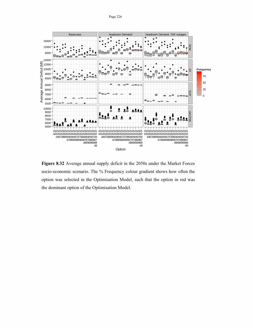
Page 226
Figure 8.32 Average annual supply deficit in the 2050s under the Market Forces
socio-economic scenario. The % Frequency colour gradient shows how often the
option was selected in the Optimisation Model, such that the option in red was
the dominant option of the Optimisation Model.
Basecase headroom Demand headroom Demand GW outages
8000
12000
16000
6000
8000
10000
12000
14000
5000
6000
7000
8000
9000
50006000700080009000
10000
RC
MF
FS
CP
UK
CP
09
d1d2
d1d2d4
d1d2d7
d1d2d8
d1d2d9
d1d2d4d7
d1d2d4d8
d1d2d4d9
d1d2d7d8
d1d2d7d9
d1d2d8d9
d1d2d4d7d8
d1d2d4d7d9
d1d2d4d8d9
d1d2d7d8d9
d1d2d4d7d8d9
d1d2
d1d2d4
d1d2d7
d1d2d8
d1d2d9
d1d2d4d7
d1d2d4d8
d1d2d4d9
d1d2d7d8
d1d2d7d9
d1d2d8d9
d1d2d4d7d8
d1d2d4d7d9
d1d2d4d8d9
d1d2d7d8d9
d1d2d4d7d8d9
d1d2
d1d2d4
d1d2d7
d1d2d8
d1d2d9
d1d2d4d7
d1d2d4d8
d1d2d4d9
d1d2d7d8
d1d2d7d9
d1d2d8d9
d1d2d4d7d8
d1d2d4d7d9
d1d2d4d8d9
d1d2d7d8d9
d1d2d4d7d8d9
Option
Ave
rag
e A
nn
ua
l De
ficit
(Ml)
0
25
50
75
Frequency
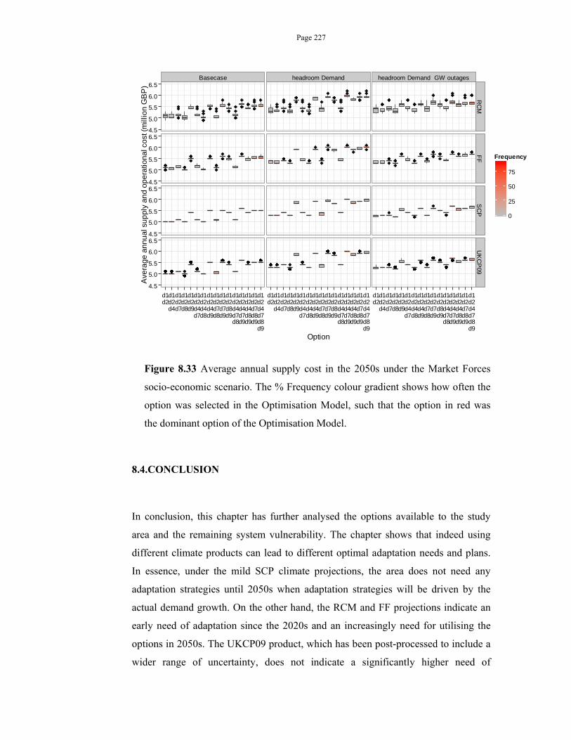
Page 227
Figure 8.33 Average annual supply cost in the 2050s under the Market Forces
socio-economic scenario. The % Frequency colour gradient shows how often the
option was selected in the Optimisation Model, such that the option in red was
the dominant option of the Optimisation Model.
8.4.CONCLUSION
In conclusion, this chapter has further analysed the options available to the study
area and the remaining system vulnerability. The chapter shows that indeed using
different climate products can lead to different optimal adaptation needs and plans.
In essence, under the mild SCP climate projections, the area does not need any
adaptation strategies until 2050s when adaptation strategies will be driven by the
actual demand growth. On the other hand, the RCM and FF projections indicate an
early need of adaptation since the 2020s and an increasingly need for utilising the
options in 2050s. The UKCP09 product, which has been post-processed to include a
wider range of uncertainty, does not indicate a significantly higher need of
Basecase headroom Demand headroom Demand GW outages
4.5
5.0
5.5
6.0
6.5
4.5
5.0
5.5
6.0
6.5
4.5
5.0
5.5
6.0
6.5
4.5
5.0
5.5
6.0
6.5
RC
MF
FS
CP
UK
CP
09
d1d2
d1d2d4
d1d2d7
d1d2d8
d1d2d9
d1d2d4d7
d1d2d4d8
d1d2d4d9
d1d2d7d8
d1d2d7d9
d1d2d8d9
d1d2d4d7d8
d1d2d4d7d9
d1d2d4d8d9
d1d2d7d8d9
d1d2d4d7d8d9
d1d2
d1d2d4
d1d2d7
d1d2d8
d1d2d9
d1d2d4d7
d1d2d4d8
d1d2d4d9
d1d2d7d8
d1d2d7d9
d1d2d8d9
d1d2d4d7d8
d1d2d4d7d9
d1d2d4d8d9
d1d2d7d8d9
d1d2d4d7d8d9
d1d2
d1d2d4
d1d2d7
d1d2d8
d1d2d9
d1d2d4d7
d1d2d4d8
d1d2d4d9
d1d2d7d8
d1d2d7d9
d1d2d8d9
d1d2d4d7d8
d1d2d4d7d9
d1d2d4d8d9
d1d2d7d8d9
d1d2d4d7d8d9
Option
Ave
rag
e a
nn
ua
l su
pp
ly a
nd
op
era
tion
al c
ost
(m
illio
n G
BP
)
0
25
50
75
Frequency
Page 228
adaptation. Indeed, the system appears to be robust under the SCP and UKCP09
conditions and with little need of additional supply or demand measure. Yet, the
system is much less robust under FF and RCM and needs the assistance of at least
universal demand metering, Arun abstraction or Ford effluent reuse. The 2020s and
2030s are still dominated by climate uncertainty, with options selected mainly due to
the different climate sources and the projected climate condition in that specific
scenario. In the 2050s, such influence interacts and is influenced by demand
uncertainty, with demand and climate uncertainty being two major controlling
factors in the Innovation, Local Resilience and Sustainable Behaviour scenarios.
However, once demand grows past the 35% threshold from the 2007 baseline
demand, it becomes the most important factor on system vulnerability and which
adaptation strategies to be selected. The extreme demand profile leads to the key
role of universal metering, desalination plant in Brighton and the combination of
Arun Abstraction, Ford effluent reuse and Wellfield optimisation in the Sussex
North area. For certain ensembles of the RCM and FF products, as well as certain
scenarios of the UKCP09 product, additional measures such as transfer
augmentation and aquifer storage and recovery in Worthing are also indicated.
Yet, the simulation model depicts a much more fragile and responsive water
resource system. In order to reduce supply deficit, the decision maker will need to
consider Arun Abstraction, Ford Effluent Reuse or a combination of Arun
Abstraction, Wellfield Optimisation and optimal demand metering. As these choices
perform quite similarly in the 2020s and the 2030s, the choice depends on the
preference of the decision makers, such as the preferred safety margin and the
financial budget. Nevertheless, the performance ranks of the options do not change
even if different climate products are used. Even with the un-bias corrected RCM
projections, the ranking is quite similar to the much more processed UKCP09. It
thus shows that while climate uncertainty dominates the uncertainty space, an
effective adaptation decision may largely reflect the local vulnerability rather than
explicitly relying on the climate products. Yet, the more robust decisions are, the
higher the operation and investment cost. Since the climate product is essential to
determine the level of supply deficit, it is essential for selecting which level of
robustness the decision makers should aim for.
Page 229
Overall, the sets of options are sufficient to reduce the area’s vulnerability under
optimization but not under simulation. The remaining deficits in transferring to
South East Water and in fulfilling the environmental flow requirements are inherent
to the Sussex delivery network attributes. In particular, there is no option that can
influence environmental flows, and the location of the transferring SEW node does
not allow for receiving water supply from other parts of the network. While this
SEW deficit does not pose direct risks to the Sussex network, it indicates that
Southern Water and South East Water need to revise their transfer agreement in
view of future climate risks. Besides, it also demonstrates that inter-regional
transfers may not be as robust as assumed. In this study, the Portsmouth transfer was
assumed to be perfectly reliable; however, its reliability in practice is dependent on
the drought extent and the supplying capacity of Portsmouth water under droughts.
Therefore, the study indicates a need for future research on inter-regional drought
risks and water operation.
Page 230
Chapter 9. ROBUST ADAPTATION PATHWAY ANALYSIS- A
DISCUSSION
9.1.REVISITING ROBUSTNESS IN THE SUSSEX CONTEXT
9.1.1. Comparison of the robustness frameworks
The previous chapters have demonstrated the cascade of uncertainty from climate
change information to the water resource planning stage. Overall, climate post-
processing and demand scenarios are two controlling uncertainty factors of the water
supply deficit level; however, the location and the level of system vulnerability are
determined by the attributes of the water delivery network and the available options.
This section revisits the concepts and frameworks of robustness as discussed in
Chapter 2; based on the results of the previous chapters, it analyses these aspects of
robustness in the context of the Sussex water resource system. It focuses on option
robustness and system robustness, which emphasise the coping range of an option
versus the overall system.
As reviewed in Chapter 2, robustness approaches in water resource planning
includes robust optimisation, real option analysis, info-gap decision theory and
robust decision making. Overall, they deviate from the traditional model of relying
on a single scenario or distribution of outcomes. Furthermore, they emphasize the
multi-source and multi-impact nature of uncertainty. Classical engineering and
statistical robustness aims to maximize the possibility of the chosen option being the
optimal strategy under imperfect information. Another robustness measure, the crisp
set approach (Rosenhead et al., 1972), meanwhile considers the number of pathways
before and after implementing a decision. As such, an option that strengthen the
supplying capacity of the system but rules out the implementation of other strategies
is considered robust by the engineering approach but not so by the crisp set
approach.
Page 231
Both of these aspects are relevant to adaptation decisions as such decisions should
cope with the present risks but also accommodate potential system transitions in the
face of uncertainty and future risks. As a combined extension of these approaches,
the Real Option approach considers the whole adaptation process as a decision tree
from which decision makers can consider trade-offs between the least-cost pathways
versus the flexibility to adapt. Meanwhile, the Info-gap Decision Theory and the
Robust Decision Making approaches focus on the uncertainty element. The former
looks at possible levels of deviation from the ‘best estimates’, in this case the
projections of climate conditions and water demand level, and gauge the option
performance against its working uncertainty zone (Korteling et al., 2013). For
instance under perfect information, option A is the optimal least-cost option;
however its performance quickly deteriorates if demand increases by 5%;
meanwhile a suboptimal option B could continue maintaining its performance up to
a demand grow by 10%. Under the Info-gap approach, option B would be identified
as a robust option instead of the option A.
Finally, the Robust Decision Making approach is distinctive compared to other
approaches due to its emphasis on vulnerability assessment. Similar to the Info-Gap
Decision Theory Approach, it considers the effectiveness of options under deep
uncertainty in the form of different scenarios. In particular, the decision makers can
state a performance threshold level above which the system is considered to be
vulnerable and the options ineffective. Additional options or alternatives are then
identified and assessed toward the goal of obtaining a satisfactory level of system
performance. For example, the decision makers may want their water system to have
no system failure under 80% of the scenarios; nevertheless under the current system,
30% of the scenarios experience system failure. The analysis then focuses on these
30% of scenarios and identifies strategies that can reduce failures to a 20% level.
Within the context of the Sussex case study, certain aspects of these robustness
approaches have been implemented in the analysis. The study combines the Robust
Optimisation approach and the Robust Decision Making approach to identify both
the optimal and the satisficing options. Moreover such a hybrid approach would help
reduce the number of option combinations (29 =512) to be considered in the Robust
Page 232
Decision Making step. The Optimisation process (Chapter 8) has produced a set of
39 option portfolios for Robust Decision Analysis. Also, instead of iteratively
consulting the decision makers on their criterion threshold, the model proceeded to
compute different criterion values using different option portfolio. As such, the
decision makers can be aware of the full range of the option performance, as well as
the associated cost. With the classical Robust Decision Making approach, the
decision maker focuses on their current preference, with this improvised approach,
they can consider changing their preference level.
In terms of constructing the demand and supply scenarios, the approach also enables
a partial application of Info-Gap Decision Analysis. Specifically for the 2050s
period, the baseline and the headroom Demand (5% increase compared to the
baseline) in the four scaling levels of the 2007 demand (namely -4%, 35%, 8% and -
15%) can represent deviations from the 2007 demand state and possible option
portfolios that work well under these ranges of deviation. Finally, by considering the
common options amongst the time periods of 2020s, 2030s and 2050s, the decision
makers can consider potential implementation pathways that balance between
drought risk reduction and system flexibility. The analysis is thus not restricted by
any pre-determined preference of robustness level and can accommodate the
decision makers’ changes in risk averseness.
9.1.2. Adaptation Robustness Analysis
9.1.2.1.Robustness to climate uncertainty and water resource uncertainty
The challenge of a changing climate is one of the key tests for adaptation decisions.
Under deep uncertainty of climate change impacts, the Sussex water resource system
has to address potential risks from drier summers and more variability in water
supplies. Overall, the Sussex system is relatively robust to the past drought patterns
but performs poorly under new drought sequences as projected by the FF ensembles.
As such, there is also an uncertainty due to climate products, in this case the
different post-processed products of the HadRM3 runs. The impacts projected by
various climate models and their ensemble members are quite diverse as illustrated
in Chapter 5. Four climate products have been considered: the original HadRM3, the
bias-corrected and downscaled RCMs from the Future Flows (FF) project, the
Page 233
Spatial Coherent Projections and the original UKCP09 change factors from the Land
Projections. They all originated from the HadRM3 projections and have undergone
different types and level of processing, and thus include different additional
uncertainty factors. Three of these products, the FF group, the SCP and the UKCP09
product, have been used in various climate impact studies for droughts and floods in
the UK. The original RCMs, meanwhile, are less used in its original form without
further bias correction in the projections or subsequent impact results. These four
different products point towards a general climate trend: compared to the 1961-1990
baseline, the period of April to September will become drier while the remaining
months will become wetter. This change in seasonal pattern is more pronounced if
the increasing trend of PET is included in the analysis. These climatic changes
subsequently affect the stream flows, in particularly the River Rother-the main
surface water source of the Sussex area. Analysis on the low flows of the River
Rother and the correlation between the observed flows and the drought indicator
SPEI shows that under dry conditions, the summer flows become strongly dependent
on the winter rainfall (refer back to Figure 6.2). As such, the Sussex water resource
system needs to plan for the diminishing summer supply. The risk from diminishing
summer supply can be abated to a certain extent by the increase in winter flows;
nevertheless the risks remain since the annual water balance is generally lower than
that of the 1961-1990 baseline period.
Aside from the climate uncertainty that these products represent, there also exists
post-processing uncertainty from different sources of information, even within the
1961-1990 baseline period. This bias was partially accounted for by comparing the
projections of each product against the baseline of the same product. Amongst the
climate products, the 10,000 realisations of the UKCP09 product demonstrate a
wider range of drought frequencies than the other 11-member products. The SCP
product, despite being described as the closest to the UKCP09 product, projects a
smaller span of drought frequencies and depending on the drought types, is within a
comparable range to the frequency ranges of the RCM and FF group. Yet, when this
post-processing uncertainty trickles down the uncertainty cascade, the UKCP09
product does not necessarily represent the most challenging conditions to the Sussex
water resource system. The vulnerability analysis in Chapter 7 shows that amongst
Page 234
the products, the Future Flows conditions exert a higher risk of supply and
environmental flow deficits compared to the UKCP09 conditions. This result was
cross-validated by both the Simulation Model and Optimisation Model of the area.
In particular, the Sussex water system appears to be robust to variations of the
droughts in the 1961-1990 periods, such as those projected by the SCP and the
UKCP09 group. While the UKCP09 and the SCP products represent climate change
impacts, they still revolve around the pattern of past droughts, in particularly the
droughts within the 1961-1990 baseline because they only provide monthly tri-
decadal changes. Both the Optimisation Model and the Simulation model
demonstrate that the most severe droughts within the SCP and the UKCP09 products
are the 1975-1976 and the 1988-1989 droughts. These are also the most serious
droughts within the 1961-1990 observed period in the Sussex area. The worst
historic event in 1921-1922 did not fall within the baseline. This robustness to past
droughts was achieved due to the current drought planning practice of the water
companies in England and Wales. In many cases, the drought plan and adaptation
decisions have been based on the worst historic droughts. Yet, when operating under
a different sequence of droughts as projected by the FF time series, the Sussex water
system is much less robust. The post-processing uncertainty also dominates
hydrological flows: even with various hydrological model parameterisations, the
flow projections are still markedly different amongst the climate products. While
these climate products do not change the ranks of performance of the adaptation
strategies in simulated results, they might lead to different preferential pathways
under optimisation. The climate products can greatly affect the level of adaptation
needs. Under the mild changes that the SCP product project, decision makers can
opt for low cost, low impact and a gradual adaptation pathway. On the other hand,
responses to higher drought risks of the FF information will require compound
supply and demand options that also incur high investment cost. As such, the post-
processing uncertainty is a major uncertainty factor in determining the adaptation
plan and pathways.
The post-processing uncertainty is also visible at the water resource model level.
The Optimisation Model considers system operation under perfect information,
while the Simulation Model demonstrates the actual risks under partial or uncertain
Page 235
information. For instance, the Optimisation Model calculates the storage of the
Weirwood Reservoir and uses groundwater licenses according to the impending
demand and supply. Therefore it can proactively plan the amount of water to be
stored in the Reservoir, as well as reserve groundwater in views of a drought.
Meanwhile the Simulation Model is rule-based and extracts the supply sources
based on the demand. Due to the difference between optimisation and simulation,
adaptation results under simulation are sensitive to the level of risks, in this case
diminishing supply due to the changes in surface flows. Therefore adaptation
planning using simulation is sensitive to climate uncertainty. Meanwhile,
optimisation can better accommodate changes in water shortage risks, but as a
consequent of these changes opts for different preferred adaptation plans.
Consequently, adaptation planning using optimisation is sensitive to both climate
uncertainty and post-processing uncertainty. Consequently, the Sussex system
appears much less robust under simulation than optimisation. In practice, as climate
uncertainty constitutes a major factor in adaptation decisions, the perfect
information state such as projected in the Optimisation Model cannot be achieved.
The system in practice is likely to be a combination of both the Optimisation Model
and the Simulation Model, as the operation of the water system could be modified
rather than fully rule-based.
9.1.2.2.Robustness to inflow changes
Overall, the Sussex system still shows a dependence on the River Rother flows and
the supply capacity is still affected by low flows. Figure 9.1 shows the 90th
percentile of daily flows (also termed Q90) (as assessed in Chapter 6) of each
scenario versus its corresponding supply deficit and operational (reported in Chapter
7 and 8). It can be seen that a scenario with a low Q90 flows tends to have higher
supply deficit than a scenario with higher Q90. This correlation is evident in the
UKCP09 group which due to its large number of 1000 realisations could highlight
the relationship between low flows and supply deficits. Chapter 8 has demonstrated
that except for the Market Forces scenario, the deficits mainly occur in the Sussex
North area, particularly in the transfer from Weirwood Reservoir to South East
Water. This deficit in the transfer cannot be alleviated by the adaptation strategies
since they are located around the Rother area and do not contribute towards the
Page 236
South East Water transfer. Therefore, this vulnerability can only be targeted by
changing the operation of Weirwood or re-negotiate the transfer agreement with
South East Water. Besides, demand management options can also be employed to
reduce the water shortage risks, particularly in dry scenarios and drought periods.
While the adaptation options can modify this relationship, the system remains
vulnerable under the dry scenarios. In essence, scenarios with Q90 being less than
100 Ml/day are likely to experience on average an annual supply deficit of 100 Ml
or more. These deficits originate from three vulnerability factors: the strong reliance
of the Sussex supply system on the River Rother, bottle-necks in the system due to
transfer capacity constraints, and the spatial distribution of the current options.
Comparison based on Figure 9.1 and 9.2 also show that the operational cost remains
fairly stable for each portfolio, therefore the chosen adaptation plan might determine
the future operational cost. They further highlight the comparative performance of
the portfolio, for instance for the 2030s, option d2 and d2-d4-d8 are expensive
options that could significantly reduce the supply deficit. However, they are of
significantly higher cost compared to other potential options. In essence, for the
2030s Base case, the d4 options could achieve a similar level of supply deficit at a
much lower cost.
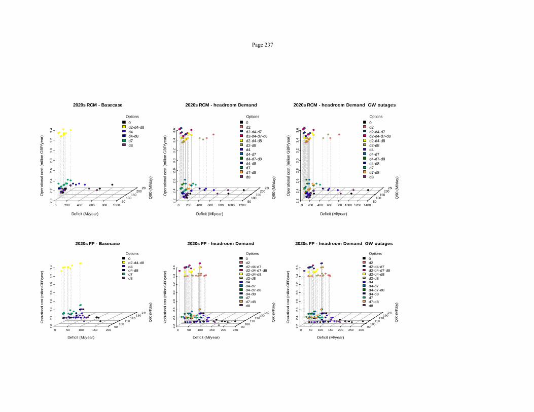
Page 237
2020s RCM - Basecase
0 200 400 600 800 1000
2.0
2.2
2.4
2.6
2.8
3.0
3.2
3.4
50100
150200
250
Deficit (Ml/year)
Q90
(M
l/day
)
Ope
ratio
nal c
ost (
milli
on G
BP
/yea
r)
Options
0d2-d4-d8d4d4-d8d7d8
2020s RCM - headroom Demand
0 200 400 600 800 1000 1200
2.2
2.4
2.6
2.8
3.0
3.2
3.4
3.6
50100
150200
250
Deficit (Ml/year)
Q90
(M
l/day
)
Ope
ratio
nal c
ost (
milli
on G
BP
/yea
r)
Options
0d2d2-d4-d7d2-d4-d7-d8d2-d4-d8d2-d8d4d4-d7d4-d7-d8d4-d8d7d7-d8d8
2020s RCM - headroom Demand GW outages
0 200 400 600 800 1000 1200 1400
2.2
2.4
2.6
2.8
3.0
3.2
3.4
3.6
50100
150200
250
Deficit (Ml/year)
Q90
(M
l/day
)
Ope
ratio
nal c
ost (
milli
on G
BP
/yea
r)
Options
0d2d2-d4-d7d2-d4-d7-d8d2-d4-d8d2-d8d4d4-d7d4-d7-d8d4-d8d7d7-d8d8
2020s FF - Basecase
0 50 100 150 200
2.0
2.2
2.4
2.6
2.8
3.0
3.2
3.4
90100
110120
130140
Deficit (Ml/year)
Q90
(M
l/day
)
Ope
ratio
nal c
ost (
milli
on G
BP/y
ear)
Options
0d2-d4-d8d4d4-d8d7d8
2020s FF - headroom Demand
0 50 100 150 200 250
2.2
2.4
2.6
2.8
3.0
3.2
3.4
3.6
90100
110120
130140
Deficit (Ml/year)
Q90
(M
l/day
)
Ope
ratio
nal c
ost (
milli
on G
BP/y
ear)
Options
0d2d2-d4-d7d2-d4-d7-d8d2-d4-d8d2-d8d4d4-d7d4-d7-d8d4-d8d7d7-d8d8
2020s FF - headroom Demand GW outages
0 50 100 150 200 250 300
2.2
2.4
2.6
2.8
3.0
3.2
3.4
3.6
90100
110120
130140
Deficit (Ml/year)
Q90
(M
l/day
)
Ope
ratio
nal c
ost (
milli
on G
BP/y
ear)
Options
0d2d2-d4-d7d2-d4-d7-d8d2-d4-d8d2-d8d4d4-d7d4-d7-d8d4-d8d7d7-d8d8
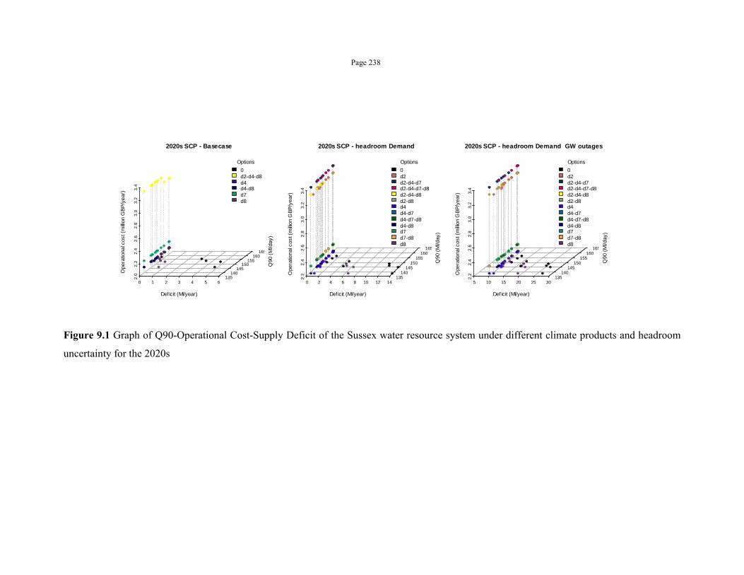
Page 238
Figure 9.1 Graph of Q90-Operational Cost-Supply Deficit of the Sussex water resource system under different climate products and headroom
uncertainty for the 2020s
2020s SCP - Basecase
0 1 2 3 4 5 6
2.0
2.2
2.4
2.6
2.8
3.0
3.2
3.4
135140
145150
155160
165
Deficit (Ml/year)
Q90
(M
l/day
)
Ope
ratio
nal c
ost (
milli
on G
BP
/yea
r)
Options
0d2-d4-d8d4d4-d8d7d8
2020s SCP - headroom Demand
0 2 4 6 8 10 12 14
2.2
2.4
2.6
2.8
3.0
3.2
3.4
135140
145150
155160
165
Deficit (Ml/year)
Q90
(M
l/day
)
Ope
ratio
nal c
ost (
milli
on G
BP
/yea
r)
Options
0d2d2-d4-d7d2-d4-d7-d8d2-d4-d8d2-d8d4d4-d7d4-d7-d8d4-d8d7d7-d8d8
2020s SCP - headroom Demand GW outages
5 10 15 20 25 30
2.2
2.4
2.6
2.8
3.0
3.2
3.4
135140
145150
155160
165
Deficit (Ml/year)
Q90
(M
l/day
)
Ope
ratio
nal c
ost (
milli
on G
BP
/yea
r)
Options
0d2d2-d4-d7d2-d4-d7-d8d2-d4-d8d2-d8d4d4-d7d4-d7-d8d4-d8d7d7-d8d8
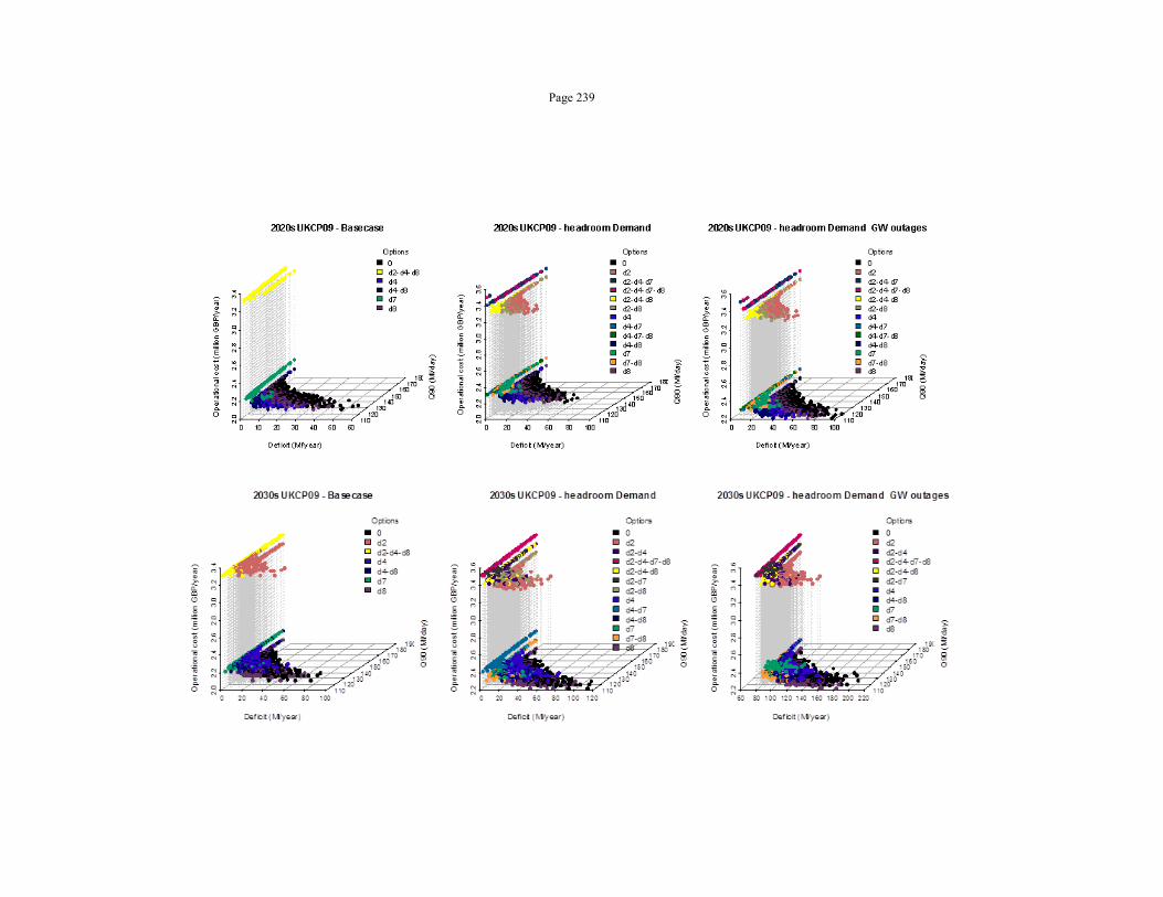
Page 239
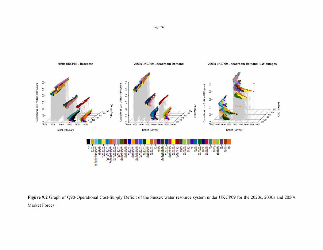
Page 240
Figure 9.2 Graph of Q90-Operational Cost-Supply Deficit of the Sussex water resource system under UKCP09 for the 2020s, 2030s and 2050s
Market Forces
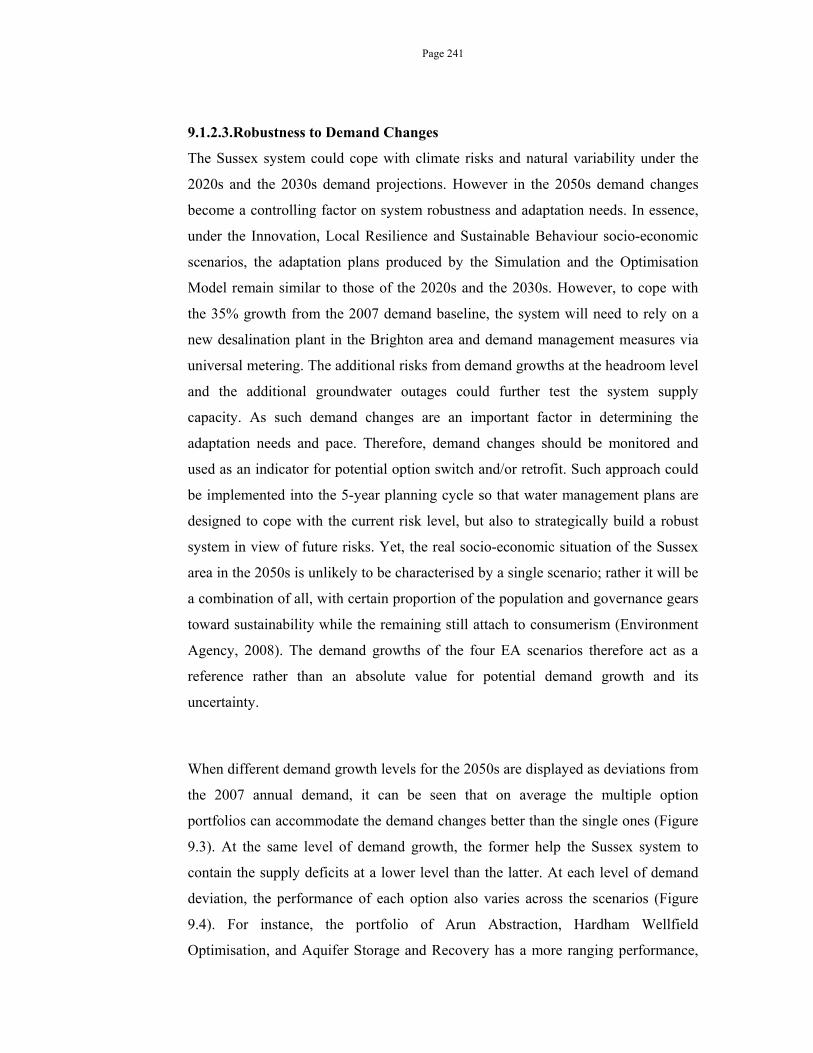
Page 241
9.1.2.3.Robustness to Demand Changes
The Sussex system could cope with climate risks and natural variability under the
2020s and the 2030s demand projections. However in the 2050s demand changes
become a controlling factor on system robustness and adaptation needs. In essence,
under the Innovation, Local Resilience and Sustainable Behaviour socio-economic
scenarios, the adaptation plans produced by the Simulation and the Optimisation
Model remain similar to those of the 2020s and the 2030s. However, to cope with
the 35% growth from the 2007 demand baseline, the system will need to rely on a
new desalination plant in the Brighton area and demand management measures via
universal metering. The additional risks from demand growths at the headroom level
and the additional groundwater outages could further test the system supply
capacity. As such demand changes are an important factor in determining the
adaptation needs and pace. Therefore, demand changes should be monitored and
used as an indicator for potential option switch and/or retrofit. Such approach could
be implemented into the 5-year planning cycle so that water management plans are
designed to cope with the current risk level, but also to strategically build a robust
system in view of future risks. Yet, the real socio-economic situation of the Sussex
area in the 2050s is unlikely to be characterised by a single scenario; rather it will be
a combination of all, with certain proportion of the population and governance gears
toward sustainability while the remaining still attach to consumerism (Environment
Agency, 2008). The demand growths of the four EA scenarios therefore act as a
reference rather than an absolute value for potential demand growth and its
uncertainty.
When different demand growth levels for the 2050s are displayed as deviations from
the 2007 annual demand, it can be seen that on average the multiple option
portfolios can accommodate the demand changes better than the single ones (Figure
9.3). At the same level of demand growth, the former help the Sussex system to
contain the supply deficits at a lower level than the latter. At each level of demand
deviation, the performance of each option also varies across the scenarios (Figure
9.4). For instance, the portfolio of Arun Abstraction, Hardham Wellfield
Optimisation, and Aquifer Storage and Recovery has a more ranging performance,
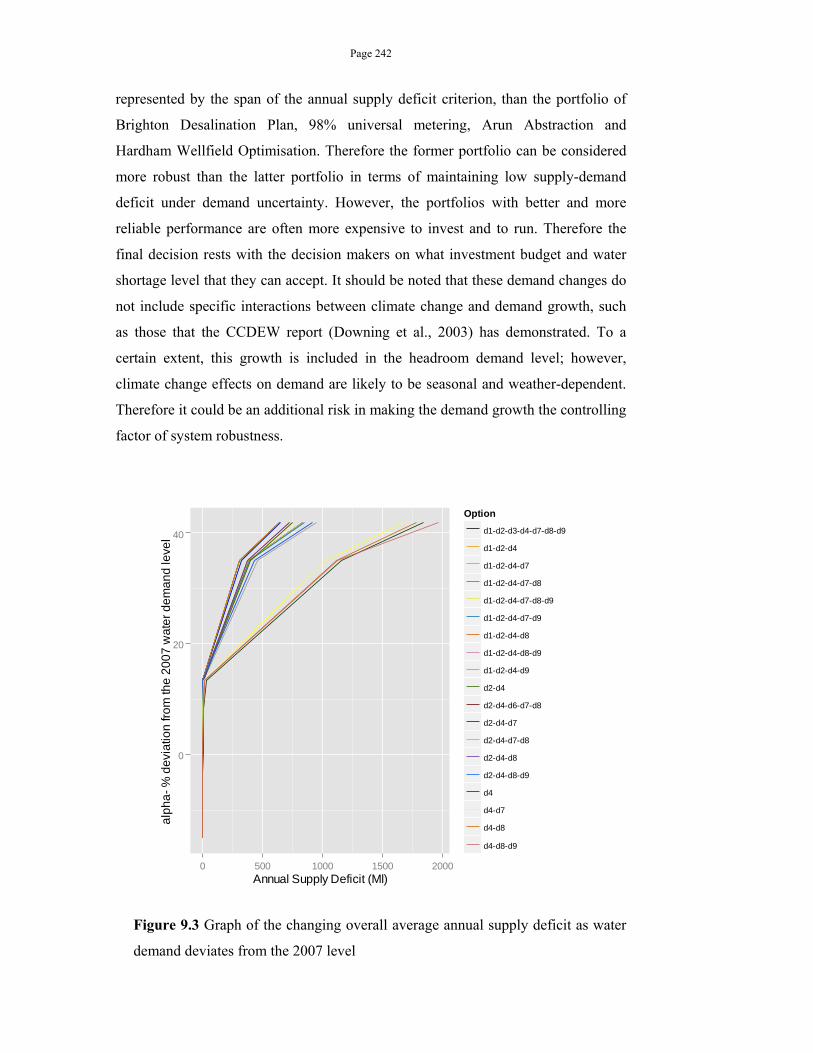
Page 242
represented by the span of the annual supply deficit criterion, than the portfolio of
Brighton Desalination Plan, 98% universal metering, Arun Abstraction and
Hardham Wellfield Optimisation. Therefore the former portfolio can be considered
more robust than the latter portfolio in terms of maintaining low supply-demand
deficit under demand uncertainty. However, the portfolios with better and more
reliable performance are often more expensive to invest and to run. Therefore the
final decision rests with the decision makers on what investment budget and water
shortage level that they can accept. It should be noted that these demand changes do
not include specific interactions between climate change and demand growth, such
as those that the CCDEW report (Downing et al., 2003) has demonstrated. To a
certain extent, this growth is included in the headroom demand level; however,
climate change effects on demand are likely to be seasonal and weather-dependent.
Therefore it could be an additional risk in making the demand growth the controlling
factor of system robustness.
Figure 9.3 Graph of the changing overall average annual supply deficit as water
demand deviates from the 2007 level
0
20
40
0 500 1000 1500 2000Annual Supply Deficit (Ml)
alp
ha-
% d
evia
tion
from
the
20
07
wat
er
dem
and
leve
l
Option
d1-d2-d3-d4-d7-d8-d9
d1-d2-d4
d1-d2-d4-d7
d1-d2-d4-d7-d8
d1-d2-d4-d7-d8-d9
d1-d2-d4-d7-d9
d1-d2-d4-d8
d1-d2-d4-d8-d9
d1-d2-d4-d9
d2-d4
d2-d4-d6-d7-d8
d2-d4-d7
d2-d4-d7-d8
d2-d4-d8
d2-d4-d8-d9
d4
d4-d7
d4-d8
d4-d8-d9
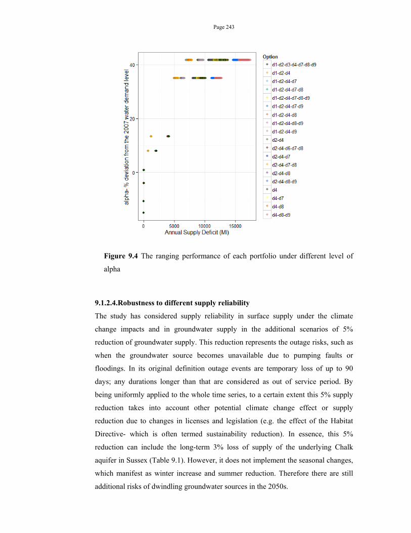
Page 243
Figure 9.4 The ranging performance of each portfolio under different level of
alpha
9.1.2.4.Robustness to different supply reliability
The study has considered supply reliability in surface supply under the climate
change impacts and in groundwater supply in the additional scenarios of 5%
reduction of groundwater supply. This reduction represents the outage risks, such as
when the groundwater source becomes unavailable due to pumping faults or
floodings. In its original definition outage events are temporary loss of up to 90
days; any durations longer than that are considered as out of service period. By
being uniformly applied to the whole time series, to a certain extent this 5% supply
reduction takes into account other potential climate change effect or supply
reduction due to changes in licenses and legislation (e.g. the effect of the Habitat
Directive- which is often termed sustainability reduction). In essence, this 5%
reduction can include the long-term 3% loss of supply of the underlying Chalk
aquifer in Sussex (Table 9.1). However, it does not implement the seasonal changes,
which manifest as winter increase and summer reduction. Therefore there are still
additional risks of dwindling groundwater sources in the 2050s.

Page 244
Table 9-1 Potential impact of climate change on groundwater by 2025. Source: Environment Agency (2009)
Overall, the modelling results in Chapter 7 and 8 show that groundwater outages do
not pose a significant risk to the Sussex area at the 2020s and 2030s water demand
level. Nevertheless it becomes a major constraint in the Market Forces 2050s since
both the Sussex Worthing and Sussex Brighton are highly dependent on
groundwater, the source of approximately 70% of their current water supply. Under
the 2020s and the 2030s situations, these groundwater sources can accommodate the
water demand, but the 2050s Market Forces level requires the need of additional
supplies from desalination. Under high demand level and groundwater outages, the
constraints on transfer capacity between Sussex North and Sussex Worthing as well
as between Sussex Worthing and Sussex Brighton can also lead to system collapse.
As most of the adaptation strategies rely on the Rother area, transferring water from
this area towards other resource zones will become a key need for future adaptation
plan. Moreover their total supply inputs are restricted by the treatment capacity of
the Hardham Water Treatment plan, which can sufficiently be reduced during
floods. Therefore, the system is at risks not only during prolonged droughts, but also
during floods. Asides from the d3 option, which enhance the transfer from the
Rother area to the Weirwood and Worthing area, the system might need further
transfer enhancement to abate the risk of demand growth and groundwater outages.
Consequently, in order to be robust to the varying reliability level of supply sources,
the system needs to implement other options than the nine options being considered
in this study, so that it can successfully cope with outages in the Worthing and
Brighton area. In this study, the transfer between Portsmouth Water and Sussex
North was assumed to be perfectly reliable. Nevertheless, water transfer amongst
water companies could still be under the threats of prolonged regional droughts. In
Page 245
the Sussex area, the transfer from Weirwood Reservoir to South East Water has been
shown to be highly susceptible to drought risks. The potential risks of transfer
failures thus should be considered in adaptation plans and further analysed in a
wider regional context.
9.1.2.5.Robustness to adaptation plan switching
Due to the richness of options, the Sussex supply system can be gradually enhanced
in its coping capacity; therefore it can accommodate the flexibility aspect of the
robustness concept. The options identified in Chapter 8 enable several adaptation
pathways. These pathways are dependent on the budget and risk averseness of the
decision makers, as well as the climate product that the plan is based on. In the
2020s, single-option plan such as universal metering (d2), smart operation of an
existing supply source (d8-Wellfield Optimisation), Arun Abstraction (d4), Ford
Effluent Reuse (d7) or a combination of d2-d4-d8 or d4-d7-d8 could enhance the
robustness of the Sussex resource system.
In practice, since the publication of the 2009 Water Resource Management Plan
(Southern Water, 2009b), the company has implemented option d4, thus orientates
the adaptation plan towards option portfolios involving the Arun Abstraction.
Therefore the company can choose to rely on d4 or additionally implement universal
metering, Wellfield Optimisation or Ford Effluent Reuse. As the adaptation needs in
the 2030s do not differ substantively to the 2020s, the decision makers can choose to
enhance their 2020s options or extend from the single or double option into a
portfolio of three options. In the 2050s, the adaptation pathways would depend on
the level of demand growth. Under the Innovation and Sustainable Behaviour
scenario, the Sussex system can still rely on its 2020s and 2030s composition. As the
Sustainable Behaviour scenario projects a lower demand level than the 2020s and
2030s, the system can even revert back to just using Wellfield Optimisation or Arun
Abstraction.
On the other hand, under the Local Resilience scenario, the system is likely in need
of additional options that have not been selected in the 2030s. To accommodate this
Page 246
8% demand growth, depending on the climate scenario, the Sussex system relies on
universal metering to reduce demand, Arun Abstraction, Ford Effluent Reuse and
additionally the Aquifer Storage Recharge in Worthing (d9). While this d9 option is
not selected in all the scenarios of UKCP09 or FF, its occurrence indicates potential
risks of shortages in Worthing that have activated the option. Overall the common
portfolios in the Local Resilience scenario should contain two or more options.
Universal metering starts to appear as a key option under this socio-economic
scenario. In contrast to other socio-economic scenarios, the Market Forces scenario
projects a steep increase in water demand and prompts the implementation of all
available adaptation options. In particular, under this scenario, universal metering
and desalination become the core strategy that occurs in every adaptation plan.
Aside from these two options, the system also needs addition implementation of d4,
d7 and d8. D4 and d7 tend to not overlap in the medium impact portfolio; these
plans often include either d4 or d7. Under headroom demand and groundwater
outage risks, the whole option set is often selected. Out of the two desalination
options for Brighton (d1 and d6), the higher capacity design were selected by the
Optimisation Model due to the severity of water shortages. As d1 and d6 are
mutually exclusive, the d6 option was not featured in the adaptation plan for the
Market Force 2050 scenarios. Overall, the potential adaptation plans across the
2020s, 2030s and 2050s period show that the Sussex system can accommodate
flexibility in their planning.
As an example, Figure 9.5 and Figure 9.6 demonstrate the potential adaptation
pathways under climate risks projected by the FF product under different demand
profiles, namely baseline demand, headroom demand and headroom demand with
groundwater outage risks. In particular, Figure 9.5 shows the most robust options,
selected as the options with the smallest worst-case scenario deficit. If there is more
than one option that can achieve that level, the selected option is the option with the
lowest investment cost. On the other hand, Figure 9.6 shows other available options
that could keep the maximum water deficit under 150 Ml/year. A comparison
between the two figures show that the most robust option is not always needed to
obtain this level of performance. Under baseline demand, while the combo of d2-d4-
d8 is the best available option for the 2020s, it is not strictly needed for the deficit
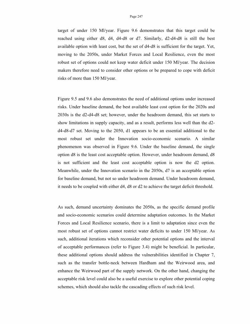
Page 247
target of under 150 Ml/year. Figure 9.6 demonstrates that this target could be
reached using either d8, d4, d4-d8 or d7. Similarly, d2-d4-d8 is still the best
available option with least cost, but the set of d4-d8 is sufficient for the target. Yet,
moving to the 2050s, under Market Forces and Local Resilience, even the most
robust set of options could not keep water deficit under 150 Ml/year. The decision
makers therefore need to consider other options or be prepared to cope with deficit
risks of more than 150 Ml/year.
Figure 9.5 and 9.6 also demonstrates the need of additional options under increased
risks. Under baseline demand, the best available least cost option for the 2020s and
2030s is the d2-d4-d8 set; however, under the headroom demand, this set starts to
show limitations in supply capacity, and as a result, performs less well than the d2-
d4-d8-d7 set. Moving to the 2050, d1 appears to be an essential additional to the
most robust set under the Innovation socio-economic scenario. A similar
phenomenon was observed in Figure 9.6. Under the baseline demand, the single
option d8 is the least cost acceptable option. However, under headroom demand, d8
is not sufficient and the least cost acceptable option is now the d2 option.
Meanwhile, under the Innovation scenario in the 2050s, d7 is an acceptable option
for baseline demand, but not so under headroom demand. Under headroom demand,
it needs to be coupled with either d4, d8 or d2 to achieve the target deficit threshold.
As such, demand uncertainty dominates the 2050s, as the specific demand profile
and socio-economic scenarios could determine adaptation outcomes. In the Market
Forces and Local Resilience scenario, there is a limit to adaptation since even the
most robust set of options cannot restrict water deficits to under 150 Ml/year. As
such, additional iterations which reconsider other potential options and the interval
of acceptable performances (refer to Figure 3.4) might be beneficial. In particular,
these additional options should address the vulnerabilities identified in Chapter 7,
such as the transfer bottle-neck between Hardham and the Weirwood area, and
enhance the Weirwood part of the supply network. On the other hand, changing the
acceptable risk level could also be a useful exercise to explore other potential coping
schemes, which should also tackle the cascading effects of such risk level.

Page 248
Figure 9.5 The most robust adaptation pathways to cope with drought risks
projected by FF. The interchange sign indicates when an option joins the portfolio.
d1
MarketForces
SustainableBehaviour
Innovation
d9
d7
d2d4d8
2020
LocalResilience
2030 2050
Co
st
d1Local
Resilience
MarketForces
SustainableBehaviour
Innovation
d9
d7
d2d4d8
d3
2020 2030 2050
Cost
Headroom Demand and Groundwater Outage Risk
Headroom Demand
Baseline Demand
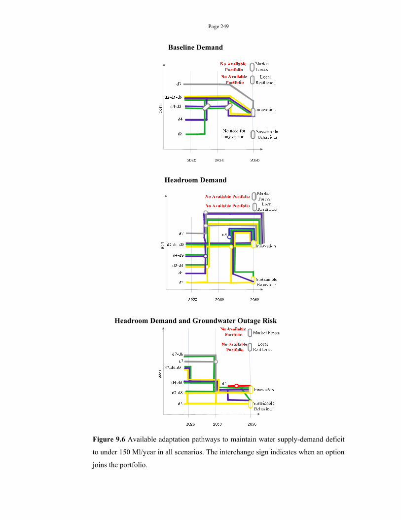
Page 249
Figure 9.6 Available adaptation pathways to maintain water supply-demand deficit
to under 150 Ml/year in all scenarios. The interchange sign indicates when an option
joins the portfolio.
Baseline Demand
Headroom Demand
Headroom Demand and Groundwater Outage Risk
Page 250
9.2.FACTORS TO ADAPTATION SUCCESS- A WIDER CONTEXT
The last section has presented robust decision analysis for the Sussex area in a
modelling context. This section subsequently aims to discuss the adaptation
decisions in a wider context, including the underlying assumptions in the modelling
process. Via an integrated assessment of the uncertainty cascade, the study has
demonstrated that the Sussex water resource system can become robust via a flexible
and sequential implementation of options. However it still remains susceptible to
potential risks from post-processing uncertainty, demand uncertainty and source
reliability uncertainty. A key feature of the current Sussex system as well as of the
future plans is the high dependency on the Rother area. Nevertheless all the supply
options in the Hardham area has to route via the Hardham Water Treatment plan,
which is still restricted by the 75 Ml/d treatment capacity. This vulnerability factor
has not yet been addressed in the current adaptation plan. Moreover the spatial
concentration of the options around this area can place additional strains on the links
and network in the Rother area. Under such strains, the link failure and leakages can
be a key impediment to adaptation success. Finally, while being presented as distinct
options in the plan, these options are still likely to connect hydrologically. In a wider
context, the area shares the Chalk aquifer with other water companies, who are also
extracting water from the rivers and the aquifer. The River Rother is quite well
connected to the underlying aquifer, and therefore its base flow can potentially be
affected by activities in its proximity or within the same aquifer. As such, the
adaptation plan should also consider other options that are located elsewhere and can
diversify the supply to the system.
Aside from the supply augmentation option, the system can also rely on demand
management to reduce the dependency on the supply side. In this study demand
management has been considered in the form of universal metering that is assumed
to reduce the demand level by 10%. However, the prospect of that reduction level is
far from clear. Until 2003, the metering statistic was only 28% and most of the
demand data was based on supply and leakage estimation. As both demand data and
leakages were estimated, they are highly unreliable. As the current metering
proportion stands at 50-70%, the new demand data have been rapidly accumulated.
Page 251
However the lack of long demand records still impedes research on the demand
pattern associating with different household demography, weather signals and
demand management measures. Deep uncertainty still plagues demand projections.
An OFWAT report in 2007 cited a UK Water Industry Research (UKWIR) study
stating that socio-economic and climate factors determine 60% of the variation in
pcc and the remaining 40% could not be explained. It was speculated to be due to
other factors, including the different pcc accounting methodologies used by
companies and data error of the demographic variable.
The current level of per capita water consumption in the Sussex area is
approximately 150 l/p/d on average and via metering is hoped to reduce to the 136
l/p/d level. The basis of the universal metering option has relied on the assumption
of reducing consumption if the users are metered and charged. Additionally
metering data will help water companies to identify the leakage locations and further
eliminate this loss. In comparison to the 2050s socio-economic scenarios, the
Innovation scenario assumes a pcc of 125 l/p/d, the Market Forces 165 l/p/d, Local
Resilience 140 l/p/d and the Sustainable Behaviour 110 l/p/d. If these assumptions
hold, universal metering could help shape the 2050s toward the Innovation or the
Local Resilience scenario. However a robust adaptation plan should not assume and
rely on automatic demand reduction via metering. There is uncertainty surrounding
whether that phenomenon of demand reduction is wide spread or can sustain over
time. In reviewing past changes, Sharp (2006) has shown literature supporting this
assumption (Baker and Toft, 2003; Jeffrey and Gearey, 2006) but also warned that
the effect varies with different groups of water users and can result in different
response pattern; domestic customers are also less likely to change their
consumption amount than commercial customers (Achttienribbe (1998) in Sharp,
2007).
An EA report on household water metering has also found price elasticity, the
changes in consumption due to 1% changes in price, of -0.14% in South East
England. The assessment by Herrington (2005) estimated a higher reduction of -0.20
to -0.25 over the summer. Based on these figures, the 10% demand reduction in the
d2 option will require a 4%-9% increase in price. While this change is comparable
Page 252
to the past price trend, its effects should be considered in a wider context of how the
consumers of different cohort will respond. According to the Consumer Council for
Water (2010), in 2009 a household in the South East spent on average £5.94 per
week and for 11.9% households, that constituted more than 3% of their expense.
Another survey by the Family Resource Survey, a survey on 25000 samples in the
UK, estimates that the average spending on water accounted for 1.8% with and 2%
without water meters of net household income. Therefore the changes in water price
and tariff should be considered with regard to its socio-economic effects. As pcc is
determined by consumption behaviour, changes in consumption at the micro level
should also be considered and accommodated. The Family Resource Survey also
shows that the household size and composition can also affect the water bills and
water pcc. With similar demographic structure, a larger household tends to have
higher water bills than a smaller household; however the average pcc of the larger
household is often less than that of the smaller one. As future household size,
demographic structure and household numbers will also affect the pcc and the
overall metered water demand, there is a need to further incorporate demand
uncertainty into future assessments.
Finally a robust adaptation decision should go beyond least-cost planning and is not
restricted by the analysis boundary. As demonstrated in Chapter 8 and Section 9.1,
both Arun Abstraction and Ford Effluent Reuse are two strong candidates for the
adaptation plan. The Arun Abstraction option was more often selected due to their
smaller investment and operational cost. Yet, in a wider context, the Ford Effluent
Reuse can offer additional benefit since it treats and recycles the effluents. It does
not extract additional water from the supply and instead increase efficiency of water
usage. It also reduces the need of large-scale infrastructures. As many water
companies now manage both water supply and effluences, the overall benefit can
outweigh the financial cost. Such added benefits however were not considered in
this study due to its focus on water supply. The adaptation pathways in this study are
likely to represent interests to cope with water supply shortages due to drought risks.
This scope while helps focus the study, may potentially affect the adaptation
capacity to other elements such as floods, water quality and the ecosystems.
Therefore robust adaptation decision making should take a holistic approach that

Page 253
integrate aspects of risks and vulnerability to the system, in order to find an
adaptation pathway that considers and accommodates all the key risks.
Page 254
Chapter 10. CONCLUSIONS AND RECOMMENDATIONS FOR
RESEARCH
At the onset of the study, the research has specified two research questions regarding
the roles of climate uncertainty in drought planning decisions and whether the
different aspects of robust decision analysis can be implemented in such assessment.
This chapter outlines the key findings, implications and recommendations arising
from the research with reference to the research aims and objectives in Chapter 1. It
summarises the results of the integrated uncertainty assessment in this study,
implications for robust adaptation decision making within the scope of the study and
beyond, as well as discussing the limitation of the research and recommendations for
future research.
10.1.REVIEW OF RESEARCH AIMS AND SUPPORTING FINDINGS
As specified in Chapter 1, the study aims to explore the components in the
uncertainty cascade from climate projections, hydrological modelling, water
resource modelling and option identification. The scope is strategy assessment of a
drought planning case study in Sussex, southeast England. The focus is uncertainty
in climate change impacts on surface water quantity and how it interacts with
hydrological modelling and socio-economic uncertainty. The research follows three
specific objectives that will be reviewed and assessed in Section 10.1.1 to 10.1.3.
10.1.1. Review different definitions and approaches of the concept of robustness
in water resource planning:
Chapter 2 has discussed the option robustness and the system robustness definition
and the approaches each group contains. In terms of characterising robustness, there
are the statistical approach, which focuses on options with the highest possibility of
being the optimal given the uncertainty; the crisp set-based approach, which
considers the number of available options before and after the decision; and the
Page 255
fuzzy set approach, which compares the system failure risks before and after a
decision. Robustness approaches in water resource planning include methodologies
as follow
Robust optimisation often treats adaptation as capacity expansion under
uncertainty, so that the system has sufficient supply capacity for projected
demand given the projected climate change impacts on water resources.
Real Option Analysis focuses on the sequential decision making given the
future options and uncertainty. The methodology emphasizes the opportunity
cost of option implementation at different decision points. For instance, it
examines the comparative Net Present Value of implementing option A at
year 1 versus year 5, and whether that decision will exclude other adaptation
pathways.
Info-gap Decision Theory explores the deterioration of strategy
performance if the climate conditions and water demand deviate from the
base case design. A robust info-gap strategy would be able to maintain its
performance to the largest bound of deviation compared to other options.
Robust Decision Making focuses on characterizing vulnerabilities of the
system under a large ensembles of scenarios and interacts with the decision
makers to identify and assess options for vulnerability reduction
These four approaches have been applied to planning problems in water resource
management. Yet, they are often applied separately. Chapter 2 has subsequently
proposed a framework that allows switching amongst the methodology depending
on the decision objectives and level of uncertainty. Chapter 7, 8 and 9 then further
engaged aspects of these approaches, by employing robust optimization and robust
decision making to identify packages of options and vulnerabilities of the Sussex
water resource system.
10.1.2. Conduct a case study in south-east England that incorporates the main
aspects of the robustness concept:
Chapter 4 to 9 have presented a case study of robust adaptation in planning practice.
The study area is the Sussex area and the scope is robust adaptation for the 2020s,
2030s and 2050s. Each of these periods was considered as a 30-year period, namely
2010-1039, 2020-2049, and 2040-2059. Aside from climate uncertainty, the study
Page 256
has integrated uncertainty from hydrological modelling, socio-economic scenarios
and water resource modelling. The climate uncertainty was represented by scenarios
and projections from different products of the Regional Climate Model HadRM3,
namely the original ensembles, the downscaled and bias-corrected ensemble from
the Future Flows project, the Spatial Coherent Projections and 1000 Latin
Hypercube samples of the UK Climate Projections UKCP09 10000 realisation. The
socio-economic scenarios for the 2050s were produced by the Environment Agency
in England and Wales and contained four scenarios, namely the Innovation, Market
Forces, Local Resilience and Sustainable Behaviour scenarios.
Overall the Sussex water supply system is susceptible to water shortage. The risks
are mild in the 2020s and 2030s, but can be significantly high under the Market
Forces scenario in the 2050s. The vulnerability mainly comes from the delivery
network attributes such as the location of major supply sources and transfer
constraints and the lack of alternative supply in certain demand nodes. Chapter 9 has
further shown that the vulnerability is strongly dependent on demand scenarios and
flow conditions. In particular, without adaptation, a 35% demand increase from the
2007 baseline will pose extreme challenges to the system and threaten a complete
supply collapse. Meanwhile Q90 low flows in the River Rother, Sussex’s major
supply source, of approximately 100 Ml/d could start to trigger water shortages in
the scenario or ensemble. Yet, the adaptation process in Sussex water management
could accommodate both aspects of the robustness concept, as well as
complementary implement different robust decision approaches.
In this study, the Robust Optimisation method was employed to identify the optimal
option set in 133 scenarios in each time slice (100 UKCP09 scenarios, 11 RCM
ensemble members, 11 FF ensemble members and 11 SCP scenarios). A Sussex
simulation model is then used to test these options under all scenarios, in essence
testing the performance of optimal options in single scenarios on the full set.
Therefore, the analysis could analyse potential ‘satisficing’ factor when an option is
not optimal in all scenarios but performs acceptably well in the sub-optimal cases to
become the robust strategy. The optimisation process was done with the objectives
being minimising environmental flow deficit, minimizing water supply deficit and
minimising the system operation and investment cost.
Page 257
The study did not indicate a specific robust measure as the recommended adaptation
plan for Sussex; instead, it presents the options along with their performance and
costs for the decision makers to select. In general, the compound options are often
more effective than single options in abating supply deficit; however, they also
entail a higher cost, which requires careful sequential planning based on system
vulnerability in the 2020s, 2030s and 2050s. Robust decision analysis in the study
indicates that the Sussex supply system can sufficiently provide water for the Sussex
North, Sussex Worthing and Sussex Brighton area in the 2020s and 2030s. The risk
of water shortage is low and can be remediated by single options of Arun
Abstraction, Ford Effluent Reuse, universal metering and Wellfield Optimisation. In
the 2050s, the Innovation and Sustainable Behaviour socio-economic scenarios still
maintain the low risks and the Sussex system can retain the composition of the
2020s and 2030s. Nevertheless, under the 8% and 35% demand growth of the Local
Resilience and Market Forces, the system will be likely under risks and need
additional strategy. Depending on the acceptable shortage risks, the system might
need to include any optimal option that it has not implemented in the 2020s and
2030s. Flexibility, or planning robustness, could be achieved since adaptation
strategies could be incrementally built over the time periods, by moving from single
option to option portfolios. Yet, the study has also shown that the current options are
not sufficiently robust under the Local Resilience and Market Forces socio-
economic scenarios. Therefore, new options aside from the current options and new
potential acceptable risk levels should be further explored.
10.1.3. Use robust decision making to demonstrate how the uncertainty
components could affect the performance of adaptation options:
Amongst the uncertainty factors investigated, demand uncertainty, climate
uncertainty and post-processing uncertainty appear to be the controlling factor. The
2020s and 2030s is dominated by climate uncertainty and climate post-processing
uncertainty. In essence, climate uncertainty in each climate product leads to the
varying performance of adaptation options. This uncertainty dominates hydrological
uncertainty of the hydrological model CATCHMOD. However, post-processing
uncertainty is also a major uncertainty element and overall could change the
preferential adaptation pathways. Under the SCP product, there is little need for the
Page 258
system to adapt to climate change impacts. Meanwhile, the FF and UKCP09 both
require incremental adaptation plans in the 2020s, 2030s and 2050s. Since the RCM
projects much drier conditions, it leads to more extreme plans and require more
strategies than other climate products; however, RCM is often not used without bias-
correction in impact studies and therefore was included only for reference in this
study. The RCM product, however, could indicate the preferential order of
adaptation options, and therefore can be used instead of other climate products if the
objective is option comparison. Moving to the 2050s, demand uncertainty becomes
the major controlling factor of adaptation options. While information and climate
uncertainty are still exhibited in the scenarios, the level of demand is the key
influence of the overall adaptation plan. Moreover, it can also affect the adaptation
pathways from the 2020s to the 2050s. In particular, under the Innovation and
Sustainable Behaviour scenarios, the adaptation pathways will mainly be single or
double options and the decision makers can rely on short-term planning or reactive
adaptation. Meanwhile, under the significant risk and requirements to adapt in the
Local Resilience and Market Forces, adaptation pathways will need to be planned
well in advance, adaptively adjusted. Under these cases, decision makers will need
to focus on system vulnerability and system renovation. Monitoring key indicators
of climate change impacts and demand growth, such as the Q90 flows and the level
of annual water demand, could also help identify potential intervention points of
option switching.
10.1.4. Key findings
The key findings of this study include
A new methodology of robust decision analysis that combines Robust
Optimisation and Robust Decision Making to include dynamic risk
preferences and the comparative option performances under certainty and
uncertainty
A case study that integrates a cascade analysis of the climate uncertainty,
climate post-processing uncertainty, hydrological uncertainty, water resource
model uncertainty and demand uncertainty on water resource planning
The recognition that climate post-processing uncertainty, in addition to other
uncertainty mentioned in the literature, can also affect the adaptation plan:

Page 259
This uncertainty has been shown to dominate other types of uncertainty for
this particular case study
An analysis that shows that vulnerability is dependent on the local conditions
and the planning option: in the Sussex case study, despite the climate post-
processing uncertainty of different climate products, main vulnerability of
the system remains similar. The vulnerability is due to the high dependence
of the system on the water sources around the Hardham area and the limited
access of these sources from other areas. Since the options are also mostly
located around this area, the Sussex water resource system remains
vulnerable in terms of maintaining the transfer agreement between Southern
Water and South East Water
A demonstration of different decision sensitive conditions that prompt option
selection under different level of water shortage: These sensitive conditions
can potentially help the decision makers to construct their adaptation plans
and pathways
10.1.5. Limitations
The study has to a great extent achieved its aims and objectives. Yet there are
several limitations remaining. Firstly, the study has not integrated hydrological
uncertainty into the final adaptation decision analysis. While climate uncertainty
dominates hydrological uncertainty overall, there is still a need to further integrate
hydrological uncertainty in future research. Secondly, the study could also further be
improved by reducing the difference in network configuration in the optimization
and the simulation model. In essence if the simulation model can accommodate a
higher resolution of the Sussex network, further comparative results on
vulnerability, particularly the vulnerability hotspot in the network, could be
conducted. Thirdly, the study has not explicitly included climate change uncertainty
in groundwater supply and demand patterns. Finally, the options considered in this
study mainly are mainly constituted of supply option. The study therefore would
benefit from an expansion of available options, in particular demand options that
engage water efficiency and rainwater harvesting.
Page 260
10.2.IMPLICATIONS FOR ADAPTATION POLICY AND PRACTICE
The study has several implications for adaptation policy and practice. Firstly, it
demonstrates that various aspects of the robustness paradigm could be implemented
in practice. The options considered in this study are management options considered
by Southern Water in their option appraisal. The study has therefore identified
robust and transformable options and pathways for the Sussex system that along
with the current planning practice, can contribute toward low vulnerability and
robust adaptation of the Sussex water resource system. Furthermore, it has
demonstrated key vulnerabilities and vulnerability threshold of the area that can help
decision makers to monitor potential need to adapt and address the issues. Overall
the study has indicated Arun Abstraction, Ford Effluent Reuse and universal
metering as core options for the adaptation plans and pathways to accumulate from.
It has also demonstrated that vulnerability is largely determined at the local level, in
this case due to the network attribute of the supply system.
In terms of practice, the study has indicated the needs to further implement demand
management and revisit assumptions regarding these measures. In terms of
methodology, the study has proposed an integrated modelling framework of robust
decision making for a large set of options. In practice, water companies often have
to consider various strategies in parallel and the original Robust Decision Making
requires a significant of model runs under such circumstance. For instance, the nine
management options of this study would have constitute 29 sets of options without a
pre-selection process; once coupled with the 1000 climate scenarios, 4 demand
profiles and 3 headroom uncertainty (the base case demand, the headroom demand
of 5% increase and the headroom demand associating with 5% groundwater
reduction), the high number of scenarios is exceedingly time and computationally
expensive. By using robust optimization to reduce the set to 39 feasible cases, the
approach shortened the simulation and analysis time to an acceptable scale to water
companies. This approach in essence will reduce the model runtime to nearly a day,
and thus, can be employed in real water planning practice. Furthermore, the study
has shown a combination of analysis originating from real option, info-gap and
Page 261
robust decision making. It therefore demonstrates their complementary application
despite their seemingly parallel ideologies.
Yet, the challenge of decision making under deep uncertainty remains. While the
study could integrate the different uncertainty components in a research study, a
similar analysis in practice is significantly time demanding, particularly when the
number of planning options explodes. Such analysis faces the challenges of
converting different climate data formats and resolutions into data that is relevant to
a water resource scale, constructing or adjusting the relevant hydrological and water
resource model, analysing the amount of data and interpreting the different
dimensions of uncertainty interactions. Therefore, in order to encourage robust
adaptation in practice, changes should be made to make data from the different
climate products readily available in an accessible and consistent format. There is
also a need for decision support tools that could integrate the uncertainty and present
the outcomes in informative visualisation and presentation.
Finally, the study has presented decision making in a holistic context, where climate
uncertainty is only one of the controlling factors of adaptation. Yet, it has shown that
with the current available climate products, adaptation pathways and decisions can
be strongly influenced by the uncertainty due to different levels of post-processing
from the same climate model results. This implies that water managers still face high
uncertainty in practice regarding which climate products to use. As demonstrated,
the UKCP09 group, while includes the highest factors of uncertainty, appears
moderately inadequate to test the system. In essence, the change factor method that
both the UKCP09 and SCP product use to project changes make the testing time
scenarios become variations of the 1961-1990 historic time series. Since hitherto
water companies still use that historic period and beyond (some even to the late
1880s), the UKCP09 and SCP essentially test water planning against the same
sequence and patterns of droughts. Meanwhile, the time series-based FF and RCM
project a wide variation of drought events and therefore present more adaptation
challenges to the system. As such, even the choice of climate product could
potentially influence the overall robustness of the system.
Page 262
10.3.RECOMMENDATION FOR FURTHER RESEARCH
As discussed before, the study still includes several limitations that can be addressed
in future research. There is a further need for holistic robust analysis approach that
incorporates climate change impacts on water demand and groundwater. That
holism should not be restricted to the modelling paradigm, but also to a bigger
picture. Various uncertainty factors such as changing behaviour and water
consumption pattern due to changes in water availability and cultural/social value
are not quantifiable and need to be considered in parallel to the modelling process.
Therefore, the study could be coupled with a qualitative assessment of vulnerability
from the perspective of relevant stakeholders for a combined modelling-social
science assessment. Such assessment will also be able to engage a wide group of
perspectives and opinions and expand the adaptation objectives beyond flows and
operational cost. Examples of additional objectives could be ecosystem services,
integrated management, risk distribution amongst the stakeholders and catchment
restoration.
Another direction of further research is the further integration of the simulation and
optimization process to reduce structure uncertainty. The model could be
constructed with internal simulation and optimization mode for a consistent network
and constraint configuration. Regarding the integrated approach of different robust
decision methods, the model can further extend the number of scenarios, such as a
bigger sample of UKCP09, to enable real option analysis along with info-gap and
RDM. Demand uncertainty and climate uncertainty could also be stochastically
generated in the simulation for a bigger set of scenarios.
Finally, future projects can investigate the nexus of resilience, robustness and
vulnerability under uncertainty. They can expand the scope to the factors
constituting adaptation success, as discussed in Chapter 1, and further identify how
uncertainty could affect these attributes and their roles.
Page 263
List of References
ACHTTIENRIBBE, G. 1998. Water price, price elasticity and the demand for drinking
water. Aqua, 47, 196-198. ADGER, N. W., ARNELL, N. W. & TOMPKINS, E. L. 2005. Successful adaptation to
climate change across scales. Global Environmental Change Part A, 15, 77-86. ADGER, W., DESSAI, S., GOULDEN, M., HULME, M., LORENZONI, I., NELSON, D.,
NAESS, L., WOLF, J. & WREFORD, A. 2009. Are there social limits to adaptation to climate change? Climatic Change, 93, 335-354.
ADGER, W. N. 2000. Social and ecological resilience: are they related? Progress in human geography, 24, 347-364.
ADGER, W. N. 2003. Social capital, collective action, and adaptation to climate change. Economic geography, 79, 387-404.
ADGER, W. N., AGRAWALA, S., MIRZA, M. M. Q., CONDE, C., O’BRIEN, K., PULHIN, J., PULWARTY, R., SMIT, B. & TAKAHASHI, K. 2007. Assessment of adaptation practices, options, constraints and capacity. Climate change, 717-743.
AJAMI, N. K., HORNBERGER, G. M. & SUNDING, D. L. 2008. Sustainable water resource management under hydrological uncertainty. Water Resour. Res, 44, 10.
ALCAMO, J. & HENRICHS, T. 2002. Critical regions: A model-based estimation of world water resources sensitive to global changes. Aquatic Sciences, 64, 352-362.
ALLAM, M. N. & ABU-RIZIAIZA, O. S. 1988. Quantification of robustness in water resource systems. Water Resources Management, 2, 231-243.
ALLEN, R. G., PEREIRA, L. S., RAES, D. & SMITH, M. 1998. Crop evapotranspiration-Guidelines for computing crop water requirements-FAO Irrigation and drainage paper 56. FAO, Rome, 300, 6541.
ALLEY, W. M. 1984. The Palmer drought severity index: limitations and assumptions. Journal of climate and applied meteorology, 23, 1100-1109.
ALLEY, W. M. 1985. THE PALMER DROUGHT SEVERITY INDEX AS A MEASURE OF HYDROLOGIC DROUGHT1. JAWRA Journal of the American Water Resources Association, 21, 105-114.
ANDERIES, J. M., JANSSEN, M. A. & OSTROM, E. 2004. A framework to analyze the robustness of social-ecological systems from an institutional perspective. Ecology and Society, 9, 18.
ARNELL, N. & CHARLTON, M. Adapting to the effects of climate change on water supply reliability. 2008.
ARNELL, N. & DELANEY, E. 2006. Adapting to climate change: public water supply in England and Wales. Climatic Change, 78, 227-255.
ARNELL, N., LIU, C., COMPAGNUCCI, R., DA CUNHA, L., HANAKI, K., HOWE, C., MAILU, G., SHIKLOMANOV, I., STAKHIV, E. & DOELL, P. 2001. Hydrology and water resources. Climate Change 2001: Impacts, Adaptation, and Vulnerability., 191-234.
ARNELL, N. W. 1999a. Climate change and global water resources. Global Environmental Change, 9, Supplement 1, S31-S49.
ARNELL, N. W. 1999b. The effect of climate change on hydrological regimes in Europe: a continental perspective. Global environmental change, 9, 5-23.
ARNELL, N. W. & CHARLTON, M. B. 2009. Adapting to the effects of climate change on water supply reliability. Adapting to climate change: thresholds, values, governance. Cambridge University Press, Cambridge.
ARNELL, N. W. & GOSLING, S. N. 2013. The impacts of climate change on river flow regimes at the global scale. Journal of Hydrology.
ATKINS LTD. 2009. Note on hydrological modelling.
Page 264
BAKER, W. & TOFT, S. 2003. A Framework Methodology for Estimating the Impact of Household Metering on Consumption, UKWIR.
BAMMER, G. & SMITHSON, M. 2008. Uncertainty and risk: multidisciplinary perspectives, Earthscan/James & James.
BARNETT, J. & O’NEILL, S. 2010. Maladaptation. Global Environmental Change, 20, 211-213.
BAUMANN, D. D., BOLAND, J. J. & HANEMANN, M. W. 1997. Urban water demand management and planning.
BEARE, D. S., AND SZAKIEL, S 2007. Managing Climate Risks – the role and value of real
options In: KULASIRI, L. O. A. D. (ed.) MODSIM 2007 International Congress on Modelling and Simulation. Modelling and Simulation Society of Australia and New Zealand, December 2007.
BELL, D., RAIFFA, H. & TVERSKY, A. 1988. Decision making: Descriptive, normative, and prescriptive interactions, Cambridge Univ Pr.
BELL, D. E. 1982. Regret in Decision Making under Uncertainty. Operations Research, 30, 961-981.
BELLARD, C., BERTELSMEIER, C., LEADLEY, P., THUILLER, W. & COURCHAMP, F. 2012. Impacts of climate change on the future of biodiversity. Ecology letters, 15, 365-377.
BELLMAN, R. 1956. Minimisation problem. Bull. Amer. Math. Soc, 62, 270. BEN-HAIM, Y. 2001. Information-gap decision theory: decisions under severe uncertainty,
Academic Pr. BEN-HAIM, Y. 2006. Info-gap decision theory: decisions under severe uncertainty,
Academic Press. BEN-TAL, A., EL GHAOUI, L. & NEMIROVSKI , A. S. 2009. Robust optimization,
Princeton Univ Pr. BEN-TAL, A. & NEMIROVSKI, A. 2002. Robust optimization – methodology and
applications. Mathematical Programming, 92, 453-480. BERKHOUT, F. & HERTIN, J. 2002. Foresight futures scenarios: developing and applying
a participative strategic planning tool. Greener Management International, 37-52. BERKHOUT, F., HERTIN, J. & JORDAN, A. 2002. Socio-economic futures in climate
change impact assessment: using scenarios as ‘learning machines’. Global Environmental Change, 12, 83-95.
BERTSIMAS, D., BROWN, D. B. & CARAMANIS, C. 2010. Theory and applications of robust optimization. Arxiv preprint arXiv:1010.5445.
BEVEN, K. 2006. A manifesto for the equifinality thesis. Journal of Hydrology, 320, 18-36. BEVEN, K. 2008. Environmental modelling: an uncertain future?, Taylor & Francis. BEVEN, K. & BINLEY, A. 1992. The future of distributed models: model calibration and
uncertainty prediction. Hydrological processes, 6, 279-298. BEVEN, K. & FREER, J. 2001. Equifinality, data assimilation, and uncertainty estimation
in mechanistic modelling of complex environmental systems using the GLUE methodology. Journal of hydrology, 249, 11-29.
BHALME, H. N. & MOOLEY, D. A. 1980. Large-scale droughts/floods and monsoon circulation. Monthly Weather Review, 108, 1197-1211.
BLENKINSOP, S. & FOWLER, H. 2007. Changes in European drought characteristics projected by the PRUDENCE regional climate models. International Journal of Climatology, 27, 1595-1610.
BOORMAN, D. B. & SEFTON, C. 1997. Recognising the uncertainty in the quantification of the effects of climate change on hydrological response. Climatic Change, 35, 415-434.
BREKKE, L. D., MILLER, N. L., BASHFORD, K. E., QUINN, N. W. & DRACUP, J. A. 2004. CLIMATE CHANGE IMPACTS UNCERTAINTY FOR WATER RESOURCES IN THE SAN JOAQUIN RIVER BASIN, CALIFORNIA1. JAWRA Journal of the American Water Resources Association, 40, 149-164.
Page 265
BRIGODE, P., OUDIN, L. & PERRIN, C. 2013. Hydrological model parameter instability: A source of additional uncertainty in estimating the hydrological impacts of climate change? Journal of Hydrology, 476, 410-425.
BROWN, C., GHILE, Y., LAVERTY, M. & LI, K. 2012. Decision scaling: Linking bottom-up vulnerability analysis with climate projections in the water sector. Water Resources Research, 48, W09537.
BROWN, C., WERICK, W., LEGER, W. & FAY, D. 2011. A Decision‐Analytic approach to managing climate risks: Application to the upper great Lakes1. JAWRA Journal of the American Water Resources Association, 47, 524-534.
BRYAN, E., DERESSA, T. T., GBETIBOUO, G. A. & RINGLER, C. 2009. Adaptation to climate change in Ethiopia and South Africa: options and constraints. environmental science & policy, 12, 413-426.
BURDETT, L., COOKSEY, E., CHRISTIE , I., WEHRMMEY, I., CHENOWETH, J. & CLIFT, R. 2006. Environment Agency scenarios 2030. Environment Agency, Bristol.
BURKE, E. J. & BROWN, S. J. 2010. Regional drought over the UK and changes in the future. Journal of Hydrology, 394, 471-485.
BUSSEY, M., CARTER, R., KEYS, N., CARTER, J., MANGOYANA, R., MATTHEWS, J., NASH, D., OLIVER, J., RICHARDS, R. & ROIKO, A. 2012. Framing adaptive capacity through a history–futures lens: Lessons from the South East Queensland Climate Adaptation Research Initiative. Futures, 44, 385-397.
BUTLER, D. & MEMON, F. A. 2006. Water demand management, International Water Assn.
BYUN, H.-R. & WILHITE, D. A. 1996. Daily quantification of drought severity and duration. Journal of Climate, 5, 1181-1201.
BYUN, H.-R. & WILHITE, D. A. 1999. Objective quantification of drought severity and duration. Journal of Climate, 12, 2747-2756.
C.G.KILSBY, H. J. F. A. 2004. Future increases in UK water resource drought projected by a regional climate model. In: B. WEBB, N. A., C. ONOF, N. MACINTYRE, R. GURNEY, C. KIRBY (ed.) Hydrology: Science and Practice for the 21st Century. Volume 1. . Proceedings of the British Hydrological Society International Conference, Imperial College.
CASHMAN, A. & LEWIS, L. 2007. Topping up or watering down? Sustainable development in the privatized UK water industry. Business Strategy and the Environment, 16, 93-105.
CAVE, M. 2009. Independent Review of Competition and Innovation in Water Markets: Final report.
CHARTERED INSTITUTION OF WATER AND ENVIRONMENTAL MANAGEMENT 2010. Regulation for a Sustainable Water Industry
A positive vision for the future water industry in England and Wales. CHEN, J., BRISSETTE, F. P. & LECONTE, R. 2011. Uncertainty of downscaling method
in quantifying the impact of climate change on hydrology. Journal of Hydrology, 401, 190-202.
CHRISTENSEN, N. & LETTENMAIER, D. 2006. A multimodel ensemble approach to assessment of climate change impacts on the hydrology and water resources of the Colorado River basin. Hydrology and Earth System Sciences Discussions Discussions, 3, 3727-3770.
CHRISTIERSON, B., VIDAL, J. P. & WADE, S. D. 2011. Using UKCP09 probabilistic climate information for UK water resource planning. Journal of Hydrology.
CHUN, K., WHEATER, H. & ONOF, C. 2013. Comparison of drought projections using two UK weather generators. Hydrological Sciences Journal, 1-15.
CHUNG, G., LANSEY, K. & BAYRAKSAN, G. 2009. Reliable water supply system design under uncertainty. Environmental Modelling & Software, 24, 449-462.
CLOKE, H., JEFFERS, C., WETTERHALL, F., BYRNE, T., LOWE, J. & PAPPENBERGER, F. 2010a. Climate impacts on river flow: projections for the
Page 266
Medway catchment, UK, with UKCP09 and CATCHMOD. Hydrological Processes.
CLOKE, H. L., JEFFERS, C., WETTERHALL, F., BYRNE, T., LOWE, J. & PAPPENBERGER, F. 2010b. Climate impacts on river flow: projections for the Medway catchment, UK, with UKCP09 and CATCHMOD. Hydrological Processes.
CLOKE, H. L., WETTERHALL, F., HE, Y., FREER, J. E. & PAPPENBERGER, F. 2012. Modelling climate impact on floods with ensemble climate projections. Quarterly Journal of the Royal Meteorological Society.
COLE, G. A., MARSH, T. J. & WALLINGFORD, U. 2006. An historical analysis of drought in England and Wales. IAHS publication, 308, 483.
COLLINS, M., BOOTH, B. B., HARRIS, G. R., MURPHY, J. M., SEXTON, D. M. & WEBB, M. J. 2006. Towards quantifying uncertainty in transient climate change. Climate Dynamics, 27, 127-147.
COMMISSION, E. 2000. The European Climate Change Programme. CONSUMER COUNCIL FOR WATER 2010. Annual Tracking Survey 2009 Report by
FDS International. COWAN, S. 1997. Competition in the water industry. Oxford review of economic policy,
13, 83-92. COWELL, P. J., THOM, B. G., JONES, R. A., EVERTS, C. H. & SIMANOVIC, D. 2006.
Management of uncertainty in predicting climate-change impacts on beaches. Journal of Coastal Research, 232-245.
DAI, A. 2011. Drought under global warming: a review. Wiley Interdisciplinary Reviews: Climate Change, 2, 45-65.
DARCH, G., ARKELL, B. & TRADEWELL, J. 2011. Water resource planning under climate uncertainty in London. Atkins Report (Reference 5103993/73/DG/035) for the Adaptation Sub-Committee and Thames Water. Atkins, Epsom.
DEPARTMENT OF ENVIRONMENT, F. A. R. A. 2011. Drought permits and drought orders. London: Water Supply and Regulation Division.
DESSAI, S. 2005. Robust adaptation decisions amid climate change uncertainties. PhD, University of East Anglia.
DESSAI, S. & HULME, M. 2004. Does climate adaptation policy need probabilities? Climate Policy, 4, 107-128.
DESSAI, S. & HULME, M. 2007. Assessing the robustness of adaptation decisions to climate change uncertainties: A case study on water resources management in the East of England. Global Environmental Change, 17, 59-72.
DESSAI, S., HULME, M., LEMPERT, R. & PIELKE JR, R. 2009. Climate prediction: a limit to adaptation? In: ADGER, W. N., LORENZONI, I. & O'BRIEN, K. L. (eds.) Adapting to Climate Change: Thresholds, values, Governance. Cambridge University Press.
DONEY, S. C., RUCKELSHAUS, M., DUFFY, J. E., BARRY, J. P., CHAN, F., ENGLISH, C. A., GALINDO, H. M., GREBMEIER, J. M., HOLLOWED, A. B. & KNOWLTON, N. 2012. Climate change impacts on marine ecosystems. Marine Science, 4.
DOWNING, T., BUTTERFIELD, R., EDMONDS, B., KNOX, J. W., MOSS, S., PIPER, B. & WEATHERHEAD, E. 2003. CCDeW: Climate Change and Demand for Water.
DRACUP, J. A., LEE, K. S. & PAULSON JR, E. G. 1980. On the definition of droughts. Water Resources Research, 16, 297-302.
DUAN, J., MCINTYRE, N. & ONOF, C. 2012. A rainfall model for drought risk analysis in south-east UK. Proceedings of the ICE - Water Management.
EL-BAROUDY, I. & SIMONOVIC, S. P. 2004. Fuzzy criteria for the evaluation of water resource systems performance. Water Resour. Res., 40, W10503.
ENVIRONMENT AGENCY 2001. Water Resources for the Future: National Report. Bristol, UK: Environment Agency.
Page 267
ENVIRONMENT AGENCY 2008. Water: Planning ahead for an uncertain future-Water in the 2050s. Bristol, UK: Environmental Agency.
ENVIRONMENT AGENCY 2009. Water for people and the environment: Water Resources Strategy for England and Wales.
ENVIRONMENT AGENCY 2011. Water Company Drought Plan Guideline. Bristol: Environment Agency.
ENVIRONMENT AGENCY, O., DEFRA AND THE WELSH GOVERNMENT 2012. Water resources planning guidelines
The technical methods and instructions. FANKHAUSER, S., SMITH, J. B. & TOL, R. S. J. 1999. Weathering climate change: some
simple rules to guide adaptation decisions. Ecological Economics, 30, 67-78. FEYEN, L. & DANKERS, R. 2009. Impact of global warming on streamflow drought in
Europe. Journal of Geophysical Research, 114, D17116. FIELD, C. B., BARROS, V., STOCKER, T. F., QIN, D., DOKKEN, D., EBI, K.,
MASTRANDREA, M., MACH, K., PLATTNER, G. & ALLEN, S. 2012. Managing the risks of extreme events and disasters to advance climate change adaptation, Cambridge University Press Cambridge.
FIERING, M. 1976. Role of Systems Analysis in Water Program Development, The. Natural Resources Journal, 16, 759-771.
FOLKE, C. 2006. Resilience: The emergence of a perspective for social–ecological systems analyses. Global Environmental Change, 16, 253-267.
FOWLER, H., BLENKINSOP, S. & TEBALDI, C. 2007. Linking climate change modelling to impacts studies: recent advances in downscaling techniques for hydrological modelling. International Journal of Climatology, 27, 1547-1578.
FOWLER, H. & KILSBY, C. 2007. Using regional climate model data to simulate historical and future river flows in northwest England. Climatic Change, 80, 337-367.
FOWLER, H., KILSBY, C. & O’CONNELL, P. 2003. Modeling the impacts of climatic change and variability on the reliability, resilience, and vulnerability of a water resource system. Water Resources Research, 39, 1222.
FOX, C., MCINTOSH, B. S. & JEFFREY, P. 2009. Classifying households for water demand forecasting using physical property characteristics. Land Use Policy, 26, 558-568.
FOXON, T. J. 2012. Transition pathways for a UK low carbon electricity future. Energy Policy.
FOXON, T. J., HAMMOND, G. P. & PEARSON, P. J. 2010. Developing transition pathways for a low carbon electricity system in the UK. Technological Forecasting and Social Change, 77, 1203-1213.
FOXON, T. J., REED, M. S. & STRINGER, L. C. 2009. Governing long‐term social–ecological change: what can the adaptive management and transition management approaches learn from each other? Environmental Policy and Governance, 19, 3-20.
FREER, J., BEVEN, K. & AMBROISE, B. 1996. Bayesian estimation of uncertainty in runoff prediction and the value of data: An application of the GLUE approach. Water Resources Research, 32, 2161-2173.
FUNKE, M. & PAETZ, M. 2011. Environmental policy under model uncertainty: a robust optimal control approach. Climatic Change, 107, 225-239.
FÜSSEL, H.-M. 2007. Vulnerability: a generally applicable conceptual framework for climate change research. Global Environmental Change, 17, 155-167.
FÜSSEL, H.-M. & KLEIN, R. J. 2006. Climate change vulnerability assessments: an evolution of conceptual thinking. Climatic Change, 75, 301-329.
GÄDEKE, A., HÖLZEL, H., KOCH, H., POHLE, I. & GRÜNEWALD, U. 2013. Analysis of uncertainties in the hydrological response of a model‐based climate change impact assessment in a subcatchment of the Spree River, Germany. Hydrological Processes.
Page 268
GAN, T. Y. 2000. Reducing vulnerability of water resources of Canadian prairies to potential droughts and possible climatic warming. Water Resources Management, 14, 111-135.
GEELS, F. W. & SCHOT, J. 2007. Typology of sociotechnical transition pathways. Research policy, 36, 399-417.
GERSONIUS, B., ASHLEY, R., PATHIRANA, A. & ZEVENBERGEN, C. 2010. Managing the flooding system's resiliency to climate change. Proceedings of the ICE-Engineering Sustainability, 163, 15-23.
GETTINGER, J., KIESLING, E., STUMMER, C. & VETSCHERA, R. 2012. A comparison of representations for discrete multi-criteria decision problems. Decision Support Systems.
GIBB, O. & RICHARDS, H. 1978. Planning for development of groundwater and surface water resources. Proceedings of the Royal Society of London. A. Mathematical and Physical Sciences, 363, 109-130.
GIBBONS, P., ZAMMIT, C., YOUNGENTOB, K., POSSINGHAM, H., LINDENMAYER, D., BEKESSY, S., BURGMAN, M., COLYVAN, M., CONSIDINE, M. & FELTON, A. 2008. Some practical suggestions for improving engagement between researchers and policy-makers in natural resource management. Ecological Management & Restoration, 9, 182-186.
GIBBS, W. & MAHER, J. 1967. Rainfall deciles as drought indicators. Commonwealth of Australia, Bureau of Meteorology, Melbourne. Bulletin.
GIORGI, F. 2008. Regionalization of climate change information for impact assessment and adaptation. Bulletin of the World Meteorological Organization, 57, 86-92.
GLEICK, P. 2000. A Look at Twenty-first Century Water Resources Development. Water International, 25, 127-138.
GOBER, P., KIRKWOOD, C., BALLING, R., ELLIS, A. & DEITRICK, S. 2010. Water Planning Under Climatic Uncertainty in Phoenix: Why We Need a New Paradigm. Annals of the Association of American Geographers, 100, 356-372.
GOMMES, R. & PETRASSI, F. 1994. Rainfall variability and drought in Sub-Saharan Africa since 1960. FAO Agrometeorology Series Working Paper.
GOODWIN, P. & WRIGHT, G. 2001. Enhancing Strategy Evaluation in Scenario Planning: a Role for Decision Analysis. Journal of Management Studies, 38, 1-16.
GREENFIELD, B. 1984. The Thames water catchment model. Unpublished Report, Technology and Development Division, Thames Water, UK.
GROTHMANN, T. & PATT, A. 2005. Adaptive capacity and human cognition: the process of individual adaptation to climate change. Global Environmental Change, 15, 199-213.
GROVES, D., YATES, D. & TEBALDI, C. 2008. Developing and applying uncertain global climate change projections for regional water management planning. Water Resour Res, 44.
GUTTMAN, N. B. 1998. Comparing the palmer drought index and the standardized precipitation index1. JAWRA Journal of the American Water Resources Association, 34, 113-121.
GUY, S. 1996. Managing water stress: the logic of demand side infrastructure planning. Journal of Environmental Planning and Management, 39, 123-130.
HALL, J., FU, G. & LAWRY, J. 2007. Imprecise probabilities of climate change: aggregation of fuzzy scenarios and model uncertainties. Climatic Change, 81, 265-281.
HALL, W. 2003. Handling uncertainty in the hydroinformatic process. Journal of Hydroinformatics, 5, 215-232.
HALLEGATTE, S. 2009. Strategies to adapt to an uncertain climate change. Global Environmental Change, 19, 240-247.
HALLEGATTE, S., SHAH, A., BROWN, C., LEMPERT, R. & GILL, S. 2012. Investment decision making under deep uncertainty--application to climate change. World Bank Policy Research Working Paper.
Page 269
HAMON, W. R. Estimating potential evapotranspiration. Proc. Amer. Soc. civ. Engrs, 1961. 107-120.
HASHIMOTO, T. 1980. Robustness, Reliability, Resilience and Vulnerability Criteria for Planning Water Resources Systems. PhD Thesis, May 1980. 125 p, 19 Fig, 10 Tab, 53 Ref, 4 Append. University Microfilms International, Ann Arbor, MI.
HASHIMOTO, T., LOUCKS, D. P. & STEDINGER, J. R. 1982a. Robustness of Water Resources Systems. Water Resources Research, 18, 21-26.
HASHIMOTO, T., STEDINGER, J. R. & LOUCKS, D. P. 1982b. Reliability, resiliency, and vulnerability criteria for water resource system performance evaluation. Water Resources Research, 18, 14-20.
HELM, D. & RAJAH, N. 1994. Water Regulation: The Periodic Review. Fiscal Studies, 15, 74-94.
HER MAJESTY’S TREASURY 2013. The Green Book: appraisal and evaluation in central government: Treasury guidance, Stationery Office.
HERRINGTON, P. 2005. Critical review of relevant research concerning the effects of charging and collection methods on water demand, different customer groups and debt. .
HINE, D. & HALL, J. W. 2010. Information gap analysis of flood model uncertainties and regional frequency analysis. Water Resour. Res., 46, W01514.
HIRSCHBOECK, K. K. 2009. Future Hydroclimatology and theResearch Challenges of a Post-Stationary World. Journal of Contemporary Water Research & Education, 142, 4-9.
HOANG, L., DESSAI, S. & BRAZIER, R. 2012. Uncertainty Analysis of an Integrated Water System in Southern England: Exploring Physical and Socio-economic Uncertainties. 2012 International Congress on Environmental Modelling and Software. Leipzig.
HOLLING, C. 1996. Engineering resilience versus ecological resilience. Foundations of Ecological Resilience, 51-66.
HOLLINGER, S., ISARD, S. & WELFORD, M. A new soil moisture drought index for predicting crop yields. Preprints, Eighth Conference on Applied Climatology, 1993. 187-190.
HOPKINS, B. 1978. The effects of the 1976 drought on chalk grassland in Sussex, England. Biological Conservation, 14, 1-12.
HOSKING, J. R. 1990. L-moments: analysis and estimation of distributions using linear combinations of order statistics. Journal of the Royal Statistical Society. Series B (Methodological), 105-124.
HOUGHTON, J. 2005. Global warming. Reports on Progress in Physics, 68, 1343. HUGGENBERGER, P., EPTING, J. & SCHEIDLER, S. 2013. Concepts for the sustainable
management of multi-scale flow systems: the groundwater system within the Laufen Basin, Switzerland. Environmental Earth Sciences, 1-17.
HUGHES, T. P., BAIRD, A. H., BELLWOOD, D. R., CARD, M., CONNOLLY, S. R., FOLKE, C., GROSBERG, R., HOEGH-GULDBERG, O., JACKSON, J. & KLEYPAS, J. 2003. Climate change, human impacts, and the resilience of coral reefs. science, 301, 929-933.
IMBERY, F., PLAGEMANN, S. & NAMYSLO, J. 2013. Processing and analysing an ensemble of climate projections for the joint research project KLIWAS. Advances in Science and Research, 10, 91-98.
INGRAM, H., MANN, D., WEATHERFORD, G. & CORTNER, H. 1984. Guidelines for improved institutional analysis in water resources planning. Water Resources Research, 20, 323-334.
IPCC 2007. Climate change 2007: impacts, adaptation and vulnerability. Cambridge University Press Cambridge.
JAIN, S., WOODHOUSE, C. A. & HOERLING, M. P. 2002. Multidecadal streamflow regimes in the interior western United States: Implications for the vulnerability of water resources. Geophysical Research Letters, 29, 32-1-32-4.
Page 270
JANSEN, M. J. 1999. Analysis of variance designs for model output. Computer Physics Communications, 117, 35-43.
JANSSEN, M. A. & ANDERIES, J. M. 2007. Robustness trade-offs in social-ecological systems. International journal of the commons, 1, 43-66.
JEFFREY, P. & GEAREY, M. 2006. Consumer reactions to water conservation policy instruments. Water Demand Management, 305, 330.
JENKINS, M. W., LUND, J. R., HOWITT, R. E., DRAPER, A. J., MSANGI, S. M., TANAKA, S. K., RITZEMA, R. S. & MARQUES, G. F. 2004. Optimization of California's water supply system: Results and insights. Journal of Water Resources Planning and Management, 130, 271-280.
JINNO, K. 1995. Risk Assessment of a Water Supply System during Drought. International Journal of Water Resources Development, 11, 185 - 204.
JONES, R. 2001. An Environmental Risk Assessment/Management Framework for Climate Change Impact Assessments. Natural Hazards, 23, 197-230.
KADANE, J. 1984. Robustness of Bayesian analyses, North Holland. KAHNEMAN, D. & TVERSKY, A. 1979. Prospect Theory: An Analysis of Decision under
Risk. Econometrica, 47, 263-291. KASPRZYK, J. R., REED, P. M., CHARACKLIS, G. W. & KIRSCH, B. R. 2012. Many-
objective de Novo water supply portfolio planning under deep uncertainty. Environmental Modelling & Software, 34, 87-104.
KATZ, R. W. & GLANTZ, M. H. 1986. Anatomy of a rainfall index. Monthly Weather Review, 114, 764-771.
KAY, A., DAVIES, H., BELL, V. & JONES, R. 2009. Comparison of uncertainty sources for climate change impacts: flood frequency in England. Climatic Change, 92, 41-63.
KAY, A. & JONES, D. 2012. Transient changes in flood frequency and timing in Britain under potential projections of climate change. International Journal of Climatology, 32, 489-502.
KEENEY, R. & RAIFFA, H. 1993. Decisions with multiple objectives: Preferences and value tradeoffs, Cambridge Univ Pr.
KELLER, K., HALL, M., KIM, S.-R., BRADFORD, D. F. & OPPENHEIMER, M. 2005. Avoiding dangerous anthropogenic interference with the climate system. Climatic Change, 73, 227-238.
KELLY, P. M. & ADGER, W. N. 2000. Theory and Practice in Assessing Vulnerability to Climate Change andFacilitating Adaptation. Climatic Change, 47, 325-352.
KENDON, E. J., ROWELL, D. P., JONES, R. G. & BUONOMO, E. 2008. Robustness of future changes in local precipitation extremes. Journal of Climate, 21, 4280-4297.
KENDON, M., MARSH, T. & PARRY, S. 2013. The 2010–2012 drought in England and Wales. Weather, 68, 88-95.
KEYANTASH, J. & DRACUP, J. A. 2002. The quantification of drought: an evaluation of drought indices. Bulletin of the American Meteorological Society, 83, 1167-1180.
KJELDSEN, T. R. & ROSBJERG, D. 2004. Choice of reliability, resilience and vulnerability estimators for risk assessments of water resources systems. Hydrological Sciences Journal, 49, 755-768.
KLINKE, A. & RENN, O. 2002. A New Approach to Risk Evaluation and Management: Risk‐Based, Precaution‐Based, and Discourse‐Based Strategies1. Risk analysis, 22, 1071-1094.
KNIGHT, F. 1921. Risk, Uncertainty and Profit. Boston and New York: Houghton Mifflin. KORTELING, B., DESSAI, S. & KAPELAN, Z. 2013. Using information-gap decision
theory for water resources planning under severe uncertainty. Water Resources Management, 27, 1149-1172.
KRIEGLER, E., HALL, J., HELD, H., DAWSON, R. & SCHELLNHUBER, H. 2009. Imprecise probability assessment of tipping points in the climate system. Proceedings of the National Academy of Sciences, 106, 5041.
Page 271
KUNDZEWICZ, Z., MATA, L., ARNELL, N. W., DÖLL, P., JIMENEZ, B., MILLER, K., OKI, T., ŞEN, Z. & SHIKLOMANOV, I. 2008. The implications of projected climate change for freshwater resources and their management.
KUNDZEWICZ, Z. W. & KINDLER, J. 1995. Multiple criteria for evaluation of reliability aspects of water resource systems. IAHS Publications-Series of Proceedings and Reports-Intern Assoc Hydrological Sciences, 231, 217-224.
LEAVESLEY, G. 1994. Modeling the effects of climate change on water resources-a review. Climatic Change, 28, 159-177.
LEMPERT, R. & GROVES, D. 2010. Identifying and evaluating robust adaptive policy responses to climate change for water management agencies in the American West. Technological Forecasting and Social Change.
LEMPERT, R., POPPER, S. & BANKES, S. 2003. Shaping the next one hundred years: New methods for quantitative, long-term policy analysis, Rand Corp.
LEMPERT, R. J. & COLLINS, M. T. 2007. Managing the Risk of Uncertain Threshold Responses: Comparison of Robust, Optimum, and Precautionary Approaches. Risk Analysis, 27, 1009-1026.
LEMPERT, R. J. & SCHLESINGER, M. E. 2000. Robust Strategies for Abating Climate Change. Climatic Change, 45, 387-401.
LINDNER, M. & KOLSTRÖM, M. A review of measures to adapt to climate change in forests of EU countries. IOP Conference Series: Earth and Environmental Science, 2009. IOP Publishing, 382007.
LINS, H. F. & COHN, T. A. 2011. Stationarity: Wanted Dead or Alive?1. JAWRA Journal of the American Water Resources Association, 47, 475-480.
LIVERMAN, D. M. 1999. Vulnerability and adaptation to drought in Mexico. Nat. Resources J., 39, 99.
LLOYD-HUGHES, B. & SAUNDERS, M. A. 2002. A drought climatology for Europe. International Journal of Climatology, 22, 1571-1592.
LOBELL, D. B., BURKE, M. B., TEBALDI, C., MASTRANDREA, M. D., FALCON, W. P. & NAYLOR, R. L. 2008. Prioritizing climate change adaptation needs for food security in 2030. Science, 319, 607-610.
LOPEZ, A., FUNG, F., NEW, M., WATTS, G., WESTON, A. & WILBY, R. 2009a. From climate model ensembles to climate change impacts and adaptation: A case study of water resource management in the southwest of England. Water Resources Research, 45, W08419.
LOPEZ, A., FUNG, F., NEW, M., WATTS, G., WESTON, A. & WILBY, R. L. 2009b. From climate model ensembles to climate change impacts and adaptation: A case study of water resource management in the southwest of England. Water Resources Research, 45, W08419-W08419.
LUSS, H. 1982. Operations research and capacity expansion problems: A survey. Operations Research, 30, 907-947.
MAGUIRE, L. & ALBRIGHT, E. 2005. Can behavioral decision theory explain risk-averse fire management decisions? Forest Ecology and Management, 211, 47-58.
MAHNOVSKI, S. 2006. Robust decisions and deep uncertainty: An application of real options to public and private investment in hydrogen and fuel cell technologies.
MAKOWSKI, M. Methodology and a modular tool for multiple criteria analysis of LP models. 1994. Citeseer.
MANNING, L., HALL, J., FOWLER, H., KILSBY, C. & TEBALDI, C. 2009. Using probabilistic climate change information from a multimodel ensemble for water resources assessment. Water Resources Research, 45, W11411.
MARSH, T. 2007. Droughts of the Past-a Preliminary Examination. CIWEM Conference-"Drought Ahead".
MARSH, T., COLE, G. & WILBY, R. 2007. Major droughts in England and Wales, 1800-2006. Weather, 62, 87-93.
MARSH, T. & TURTON, P. 1996. The 1995 drought—a water resources perspective. Weather, 51, 46-53.
Page 272
MARSH, T. J. 2004. The UK Drought of 2003-An Overview (extended version of paper in Weather, 59. No.8, 224-230). Wallingford: Centre for Ecology and Hydrology.
MARVIN, S., CHAPPELLS, H. & GUY, S. 1999. Pathways of smart metering development: shaping environmental innovation. Computers, Environment and Urban Systems, 23, 109-126.
MATROSOV, E. S., HAROU, J. J. & LOUCKS, D. P. 2011. A computationally efficient open-source water resource system simulator–Application to London and the Thames Basin. Environmental Modelling & Software, 26, 1599-1610.
MATROSOV, E. S., PADULA, S. & HAROU, J. J. 2012. Selecting Portfolios of Water Supply and Demand Management Strategies Under Uncertainty—Contrasting Economic Optimisation and ‘Robust Decision Making’ Approaches. Water Resources Management, 27, 1123-1148.
MATROSOV, E. S., PADULA, S. & HAROU, J. J. 2013. Selecting Portfolios of Water Supply and Demand Management Strategies Under Uncertainty—Contrasting Economic Optimisation and ‘Robust Decision Making’Approaches. Water Resources Management, 27, 1123-1148.
MAURER, E. 2007. Uncertainty in hydrologic impacts of climate change in the Sierra Nevada, California, under two emissions scenarios. Climatic Change, 82, 309-325.
MCCARTHY, J. 2001. Climate change 2001: impacts, adaptation, and vulnerability: contribution of Working Group II to the third assessment report of the Intergovernmental Panel on Climate Change, Cambridge Univ Pr.
MCGUINNESS, J. L. & BORDNE, E. F. 1972. A comparison of lysimeter-derived potential evapotranspiration with computed values, US Dept. of Agriculture.
MCKEE, T. B., DOESKEN, N. J. & KLEIST, J. The relationship of drought frequency and duration to time scales. Proceedings of the 8th Conference on Applied Climatology, 1993. American Meteorological Society Boston, MA, 179-183.
MCKEE, T. B., DOESKEN, N. J. & KLEIST, J. Drought monitoring with multiple time scales. Ninth Conference on Applied Climatology. American Meteorological Society, Boston, 1995.
MCMAHON, T. & ARENAS, A. D. 1982. Methods of computation of low streamflow, Unesco.
MEDD, W. & CHAPPELLS, H. 2007. Drought, demand and the scale of resilience: challenges for interdisciplinarity in practice. Interdisciplinary Science Reviews, 32, 233-248.
MEYER, S. & HUBBARD, K. Extending the crop-specific drought index to soybean. Preprints, Ninth Conference on Applied Climatology, 1995. 233-236.
MILLY, P. C. D., BETANCOURT, J., FALKENMARK, M., HIRSCH, R. M., KUNDZEWICZ, Z. W., LETTENMAIER, D. P. & STOUFFER, R. J. 2008. Stationarity Is Dead: Whither Water Management? Science, 319, 573-574.
MINVILLE, M., BRISSETTE, F. & LECONTE, R. 2010. Impacts and Uncertainty of Climate Change on Water Resource Management of the Peribonka River System (Canada). Journal of Water Resources Planning and Management-Asce, 136, 376-385.
MOREIRA, E. E., PAULO, A. A. & PEREIRA, L. S. 2007. Is Drought Occurrence And Severity Increasing Due to Climate Change? Analysing Drought Class Transitions With Loglinear Models. Methods and Tools for Drought Analysis and Management.
MORGENSTERN, O. & VON NEUMANN, J. 1947. Theory of games and economic behavior, Princeton University Press Princeton, NJ.
MORID, S., SMAKHTIN, V. & MOGHADDASI, M. 2006. Comparison of seven meteorological indices for drought monitoring in Iran. International Journal of Climatology, 26, 971-985.
MOY, W. S., COHON, J. L. & REVELLE, C. S. 1986. A programming model for analysis of the reliability, resilience, and vulnerability of a water supply reservoir. Water Resources Research, 22, 489-498.
Page 273
MPELASOKA, F., HENNESSY, K., JONES, R. & BATES, B. 2008. Comparison of suitable drought indices for climate change impacts assessment over Australia towards resource management. International Journal of Climatology, 28, 1283-1292.
MYERS, S. C. 1984. Finance Theory and Financial Strategy. Interfaces, 14, 126-137. NAIMAN, R. J., BUNN, S. E., NILSSON, C., PETTS, G. E., PINAY, G. & THOMPSON,
L. C. 2002. Legitimizing Fluvial Ecosystems as Users of Water: An Overview. Environmental Management, 30, 455-467.
NAKICENOVIC, N., ALCAMO, J., DAVIS, G., DE VRIES, B., FENHANN, J., GAFFIN, S., GREGORY, K., GRUBLER, A., JUNG, T. Y. & KRAM, T. 2000. Special report on emissions scenarios: a special report of Working Group III of the Intergovernmental Panel on Climate Change. Pacific Northwest National Laboratory, Richland, WA (US), Environmental Molecular Sciences Laboratory (US).
NELSON, D. R., ADGER, W. N. & BROWN, K. 2007. Adaptation to environmental change: contributions of a resilience framework. Annu. Rev. Environ. Resour., 32, 395-419.
NĚMEC, J. & SCHAAKE, J. 1982. Sensitivity of water resource systems to climate variation. Hydrological Sciences Journal, 27, 327-343.
NEW, M., LOPEZ, A., DESSAI, S. & WILBY, R. 2007. Challenges in using probabilistic climate change information for impact assessments: an example from the water sector. Philosophical Transactions of the Royal Society A: Mathematical, Physical and Engineering Sciences, 365, 2117.
NIEMEYER, S., PETTS, J. & HOBSON, K. 2005. Rapid climate change and society: assessing responses and thresholds. Risk Analysis, 25, 1443-1456.
NOWOTNY, H. 1999. The need for socially robust knowledge. TA-Datenbank-Nachrichten, 8, 12-16.
NOWOTNY, H. 2003. Re-thinking science: From reliable knowledge to socially robust knowledge. Entangled histories and negotiated universals: centers and peripheries in a changing world, 14.
O'BRIEN, K. L., ERIKSEN, S., SCHJOLDEN, A. & NYGAARD, L. 2009. What’s in a word? Conflicting interpretations of vulnerability in climate change research.
O'NEILL, H. M., POUDER, R. W. & BUCHHOLTZ, A. K. 1998. Patterns in the diffusion of strategies across organizations: insights from the innovation diffusion literature. Academy of Management Review, 23, 98-114.
O’HARA, J. K. & GEORGAKAKOS, K. P. 2008. Quantifying the urban water supply impacts of climate change. Water Resources Management, 22, 1477-1497.
OGDEN, S. & WATSON, R. 1999. Corporate Performance and Stakeholder Management: Balancing Shareholder and Customer Interests in the U.K. Privatized Water Industry. The Academy of Management Journal, 42, 526-538.
OKI, T. & KANAE, S. 2006. Global hydrological cycles and world water resources. science, 313, 1068-1072.
OLSTON, C. & MACKINLAY, J. D. Visualizing data with bounded uncertainty. 2002. IEEE, 37-40.
OUDIN, L., HERVIEU, F., MICHEL, C., PERRIN, C., ANDRÉASSIAN, V., ANCTIL, F. & LOUMAGNE, C. 2005. Which potential evapotranspiration input for a lumped rainfall–runoff model?: Part 2—Towards a simple and efficient potential evapotranspiration model for rainfall–runoff modelling. Journal of Hydrology, 303, 290-306.
PAAVOLA, J. & ADGER, W. N. 2006. Fair adaptation to climate change. Ecological Economics, 56, 594-609.
PAHL-WOSTL, C. 2002. Towards sustainability in the water sector – The importance of human actors and processes of social learning. Aquatic Sciences - Research Across Boundaries, 64, 394-411.
Page 274
PAHL-WOSTL, C. 2007. Transitions towards adaptive management of water facing climate and global change. Water Resources Management, 21, 49-62.
PAHL-WOSTL, C., SENDZIMIR, J., JEFFREY, P., AERTS, J., BERKAMP, G. & CROSS, K. 2007. Managing change toward adaptive water management through social learning. Ecology and Society, 12, 30.
PALMER, W. C. 1965. Meteorological drought, US Department of Commerce, Weather Bureau Washington, DC, USA.
PALMER, W. C. 1968. Keeping track of crop moisture conditions, nationwide: The new crop moisture index.
PANEL ON WATER AND CLIMATE, G. S. C. 1977. Climate, Climatic Change, and Water Supply. Geophysics Research Board, National Research Council.
PARKER, D. 1999. Regulation of privatised public utilities in the UK: performance and governance. International Journal of Public Sector Management, 12, 213-236.
PARMIGIANI, G. & INOUE, L. 2009. Decision theory: principles and approaches. PARRY, M. L., CANZIANI, O., PALUTIKOF, J., VAN DER LINDEN, P. & HANSON,
C. 2007. Climate Change 2007: Impacts, Adaptation and Vulnerability: Working Group I Contribution to the Fourth Assessment Report of the IPCC, Cambridge University Press.
PARSON, E., BURKETT, V., FISHER-VANDEN, K., KEITH, D., MEARNS, L., PITCHER, H., ROSENZWEIG, C. & WEBSTER, M. 2007. Global-change scenarios: their development and use. US Department of Energy Publications, 7.
PATON, F., MAIER, H. & DANDY, G. 2013. Relative magnitudes of sources of uncertainty in assessing climate change impacts on water supply security for the Southern Adelaide water supply system. Water Resources Research.
PEEL, M. C. & BLÖSCHL, G. 2011. Hydrological modelling in a changing world. Progress in Physical Geography, 35, 249-261.
PELLING, M. 2011. Adaptation to climate change: from resilience to transformation, Taylor & Francis US.
PETERSON, T., WESTERN, A. & ARGENT, R. 2012. Analytical methods for ecosystem resilience: A hydrological investigation. Water Resources Research, 48, W10531.
PHILLIPS, I. D. & MCGREGOR, G. R. 1998. The utility of a drought index for assessing the drought hazard in Devon and Cornwall, South West England. Meteorological Applications, 5, 359-372.
PITTOCK, A. & JONES, R. 2000. Adaptation to what and why? Environmental Monitoring and Assessment, 61, 9-35.
PLANNING & CLIMATE CHANGE COALITION 2010. Planning for climate change-Guidance and model policies for local authorities.
POFF, N., ALLAN, J., PALMER, M., HART, D., RICHTER, B., ARTHINGTON, A., ROGERS, K., MEYER, J. & STANFORD, J. 2003. River flows and water wars: emerging science for environmental decision making. Frontiers in Ecology and the Environment, 1, 298-306.
PRUDHOMME, C. & DAVIES, H. 2009. Assessing uncertainties in climate change impact analyses on the river flow regimes in the UK. Part 2: future climate. Climatic Change, 93, 197-222.
PRUDHOMME, C., FARQUHARSON, F., AGENCY, E., ECOLOGY, C. F. & HYDROLOGY 2003. Probability distributions for long period rainfall: a scoping study, Environment Agency.
PRUDHOMME, C., WILBY, R. L., CROOKS, S., KAY, A. L. & REYNARD, N. S. 2010. Scenario-neutral approach to climate change impact studies: Application to flood risk. Journal of Hydrology, 390, 198-209.
PRUDHOMME, C., YOUNG, A., WATTS, G., HAXTON, T., CROOKS, S., WILLIAMSON, J., DAVIES, H., DADSON, S. & ALLEN, S. 2012. The drying up of Britain? A national estimate of changes in seasonal river flows from 11 Regional Climate Model simulations. Hydrological Processes, 26, 1115-1118.
PUJOL , G., IOOSS, B. & JANON, A. 2013. R package 'sensitivity'. Version 1.7. CRAN.
Page 275
QUIRING, S. M. & PAPAKRYIAKOU, T. N. 2003. An evaluation of agricultural drought indices for the Canadian prairies. Agricultural and Forest Meteorology, 118, 49-62.
RAHIZ, M. & NEW, M. 2013. 21st Century Drought Scenarios for the UK. Water Resources Management, 27, 1039-1061.
RANDALL, D. A., WOOD, R. A., BONY, S., COLMAN, R., FICHEFET, T., FYFE, J., KATTSOV, V., PITMAN, A., SHUKLA, J. & SRINIVASAN, J. 2007. Climate models and their evaluation. Climate change, 323.
RANGER, N., MILLNER, A., DIETZ, S., FANKHAUSER, S., LOPEZ, A. & RUTA, G. 2010. Adaptation in the UK: a decision-making process, Environment Agency.
RAY, P., VOGEL, R. & WATKINS, D. Robust Optimization Using a Variety of Performance Indices. ASCE, 4710-4719.
RAYNER, N., BROHAN, P., PARKER, D., FOLLAND, C., KENNEDY, J., VANICEK, M., ANSELL, T. & TETT, S. 2006. Improved analyses of changes and uncertainties in sea surface temperature measured in situ since the mid-nineteenth century: The HadSST2 dataset. Journal of Climate, 19, 446-469.
RISBEY, J. S. 1998. Sensitivities of water supply planning decisions to streamflow and climate scenario uncertainties. Water Policy, 1, 321-340.
RODRIGUES, H., GUEDES, J. M. & BENDSOE, M. 2002. Hierarchical optimization of material and structure. Structural and Multidisciplinary Optimization, 24, 1-10.
ROSENHEAD, J., ELTON, M. & GUPTA, S. K. 1972. Robustness and Optimality as Criteria for Strategic Decisions. Operational Research Quarterly (1970-1977), 23, 413-431.
ROSETA-PALMA, C. & XEPAPADEAS, A. 2004. Robust Control in Water Management. Journal of Risk and Uncertainty, 29, 21-34.
SAAL, D. S. & PARKER, D. 2000. The impact of privatization and regulation on the water and sewerage industry in England and Wales: a translog cost function model. Managerial and Decision Economics, 21, 253-268.
SADOFF, C. W. & GREY, D. 2002. Beyond the river: the benefits of cooperation on international rivers. Water policy, 4, 389-403.
SALINGER, M. 2005. Climate Variability and Change: Past, Present and Future – An Overview. Climatic Change, 70, 9-29.
SALTELLI, A. 2002. Making best use of model evaluations to compute sensitivity indices. Computer Physics Communications, 145, 280-297.
SALTELLI, A., ANNONI, P., AZZINI, I., CAMPOLONGO, F., RATTO, M. & TARANTOLA, S. 2010. Variance based sensitivity analysis of model output. Design and estimator for the total sensitivity index. Computer Physics Communications, 181, 259-270.
SALTELLI, A., CHAN, K. & SCOTT, E. M. 2000. Sensitivity analysis, Wiley New York. SCIENCE AND TECHNOLOGY POLICY RESEARCH 2002. Foresight Futures: 2020
revised scenarios and guidance. SPRU, University of Sussex, Brighton, UK. SEXTON , M. H. D., HARRIS, G. & MURPHY, J. 2010. UKCP09: Spatially coherent
projections. UKCP09 additional product. SHARP, L. 2006. Water demand management in England and Wales: Constructions of the
domestic water user. Journal of Environmental Planning and Management, 49, 869-889.
SHIAU, J. T. & LEE, H. C. 2005. Derivation of Optimal Hedging Rules for a Water-supply Reservoir through Compromise Programming. Water Resources Management, 19, 111-132.
SIMON, H. 1979. Rational decision making in business organizations. The American economic review, 69, 493-513.
SIMONOVIC, S. P. & VERMA, R. 2008. A new methodology for water resources multicriteria decision making under uncertainty. Physics and Chemistry of the Earth, Parts A/B/C, 33, 322-329.
Page 276
SMAKHTIN, V. & HUGHES, D. 2007. Automated estimation and analyses of meteorological drought characteristics from monthly rainfall data. Environmental Modelling & Software, 22, 880-890.
SMIT, B., BURTON, I., KLEIN, R. J. & WANDEL, J. 2000. An anatomy of adaptation to climate change and variability, Springer.
SMIT, B. & PILIFOSOVA, O. 2003. From adaptation to adaptive capacity and vulnerability reduction. Climate change, adaptive capacity and development, 9-28.
SMIT, B. & WANDEL, J. 2006. Adaptation, adaptive capacity and vulnerability. Global environmental change, 16, 282-292.
SMITHERS, J. & SMIT, B. 1997. Human adaptation to climatic variability and change. Global Environmental Change, 7, 129-146.
SOBOL', I. Y. M. 1990. On sensitivity estimation for nonlinear mathematical models. Matematicheskoe Modelirovanie, 2, 112-118.
SOBOL, I., TARANTOLA, S., GATELLI, D., KUCHERENKO, S. & MAUNTZ, W. 2007. Estimating the approximation error when fixing unessential factors in global sensitivity analysis. Reliability Engineering & System Safety, 92, 957-960.
SOBOL, I. M. 1993. Sensitivity estimates for nonlinear mathematical models. Mathematical Modelling and Computational Experiments, 1, 407-414.
SOUTHERN WATER 2009a. Business Plan 2010-2015: Balancing the needs of customers in a changing environment.
SOUTHERN WATER 2009b. Water Resources Management Plan. SOUTHERN WATER 2013. Drought Plan. SRDJEVIC, B., MEDEIROS, Y. D. P. & FARIA, A. S. 2004. An Objective Multi-Criteria
Evaluation of Water Management Scenarios. Water Resources Management, 18, 35-54.
STAINFORTH, D., ALLEN, M., TREDGER, E. & SMITH, L. A. 2007a. Confidence, uncertainty and decision-support relevance in climate predictions. Philosophical Transactions of the Royal Society A: Mathematical, Physical and Engineering Sciences, 365, 2145.
STAINFORTH, D. A., DOWNING, T. E., WASHINGTON, R., LOPEZ, A. & NEW, M. 2007b. Issues in the interpretation of climate model ensembles to inform decisions. Philosophical Transactions of the Royal Society A: Mathematical, Physical and Engineering Sciences, 365, 2163.
STERN, N. 2007. The Economics of Climate Change: The Stern Review, Cambridge, Cambridge University Press.
SUBAK, S. 2000. Climate Change Adaptation in the U.K. Water Industry: Managers' Persceptions of Past Variability and Future Scenarios. Water Resources Management, 14, 137-156.
THOMALLA, F., DOWNING, T., SPANGER‐SIEGFRIED, E., HAN, G. & ROCKSTRÖM, J. 2006. Reducing hazard vulnerability: towards a common approach between disaster risk reduction and climate adaptation. Disasters, 30, 39-48.
THOMPSON, M. 2003. Cultural theory, climate change and clumsiness. Economic and Political Weekly, 5107-5112.
THOMPSON, M., ELLIS, R., WILDAVSKY, A. B. & THOMPSON, M. 1990. Cultural theory, Westview Press Boulder.
THOMPSON, N., BARRIE, I., AYLES, M. & BRITAIN, G. 1981. The Meteorological Office rainfall and evaporation calculation system: MORECS (July 1981), Meteorological Office.
THORNTHWAITE, C. W. 1948. An approach toward a rational classification of climate. Geographical review, 38, 55-94.
TOMPKINS, E. L. & ADGER, W. 2004. Does adaptive management of natural resources enhance resilience to climate change? Ecology and society, 9, 10.
Page 277
TU, M.-Y., HSU, N.-S., TSAI, F. T. C. & YEH, W. W. G. 2008. Optimization of Hedging Rules for Reservoir Operations. Journal of Water Resources Planning and Management, 134, 3-13.
UK WATER INDUSTRY RESEARCH 1998. A practical method fo converting uncertainty into headroom. 98/WR/13/1. London: UK water Industry Research Ltd.
VAN DER BRUGGE, R. & VAN RAAK, R. 2007. Facing the adaptive management challenge: insights from transition management. Ecology and Society, 12, 33.
VAN ROOY, M. 1965. A rainfall anomaly index independent of time and space. Notos, 14, 43-48.
VANNITSEM, S. 2011. Bias correction and post-processing under climate change. Nonlin. Processes Geophys., 18, 911-924.
VICENTE-SERRANO, S. M., BEGUERÍA, S. & LÓPEZ-MORENO, J. I. 2010. A multiscalar drought index sensitive to global warming: the standardized precipitation evapotranspiration index. Journal of Climate, 23, 1696-1718.
VIDAL, J. P. & WADE, S. 2009. A multimodel assessment of future climatological droughts in the United Kingdom. International Journal of Climatology, 29, 2056-2071.
VOGEL, C., MOSER, S. C., KASPERSON, R. E. & DABELKO, G. D. 2007. Linking vulnerability, adaptation, and resilience science to practice: Pathways, players, and partnerships. Global Environmental Change, 17, 349-364.
VON WINTERFELDT, D. & EDWARDS, W. 1986. Decision analysis and behavioral research, Cambridge University Press Cambridge.
VÖRÖSMARTY, C. J., GREEN, P., SALISBURY, J. & LAMMERS, R. B. 2000. Global water resources: vulnerability from climate change and population growth. science, 289, 284.
WADE, S. D. 2005. Model Note of the Sussex North Excel Model. WADE, S. D., JONES, P. D. & OSBORN, T. 2006. The impacts of climate change on
severe droughts. Implications for decision making. . Environment Agency. WADE, S. D., RANCE, J. & REYNARD, N. 2013. The UK climate change risk assessment
2012: assessing the impacts on water resources to inform policy makers. Water Resources Management, 27, 1085-1109.
WALKER, W., HAASNOOT, M. & KWAKKEL, J. 2013. Adapt or Perish: A Review of Planning Approaches for Adaptation under Deep Uncertainty. Sustainability, 5, 955-979.
WANG, T. & DE NEUFVILLE, R. Building real options into physical systems with stochastic mixed-integer programming. 8th Real Options Annual International Conference, June 2004 2004 Montreal, Canada. Citeseer.
WATER FRAMEWORK DIRECTIVE 2000. Directive 2000/60. EC of the European Parliament and of the Council of, 23, 1.
WATER RESOURCES IN THE SOUTH EAST GROUP 2010. Progress towards a shared water resources strategy in the South East of England.
WATKINS, D. W. & MCKINNEY, D. C. 1995. Robust optimization for incorporating risk and uncertainty in sustainable water resources planning. IAHS Publications-Series of Proceedings and Reports-Intern Assoc Hydrological Sciences, 231, 225-232.
WATKINS JR, D. W. 1997. Finding robust solutions to water resources problems. Journal of Water Resources Planning and Management, 123, 49.
WEAVER, C. P., LEMPERT, R. J., BROWN, C., HALL, J. A., REVELL, D. & SAREWITZ, D. 2013. Improving the contribution of climate model information to decision making: the value and demands of robust decision frameworks. Wiley Interdisciplinary Reviews: Climate Change, 4, 39-60.
WEGHORST, K. The reclamation drought index: guidelines and practical applications. North American Water and Environment Congress & Destructive Water, 1996. ASCE, 637-642.
Page 278
WERRITTY, A. 2002. Living with uncertainty: climate change, river flows and water resource management in Scotland. The Science of the Total Environment, 294, 29-40.
WIGLEY, T. & ATKINSON, T. 1977. Dry years in south-east England since 1698. WILBY, R. 2005. Uncertainty in water resource model parameters used for climate change
impact assessment. Hydrological Processes, 19, 3201-3219. WILBY, R. & DESSAI, S. Robust adaptation to climate change. Weather, 65, 180-185. WILBY, R., GREENFIELD, B. & GLENNY, C. 1994. A coupled synoptic-hydrological
model for climate change impact assessment. Journal of Hydrology, 153, 265-290. WILBY, R., TRONI, J., BIOT, Y., TEDD, L., HEWITSON, B., SMITH, D. & SUTTON, R.
2009. A review of climate risk information for adaptation and development planning. International Journal of Climatology, 29, 1193-1215.
WILBY, R., WHITEHEAD, P., WADE, A., BUTTERFIELD, D., DAVIS, R. & WATTS, G. 2006. Integrated modelling of climate change impacts on water resources and quality in a lowland catchment: River Kennet, UK. Journal of Hydrology, 330, 204-220.
WILBY, R. L. & HARRIS, I. 2006. A framework for assessing uncertainties in climate change impacts: Low-flow scenarios for the River Thames, UK. Water Resour. Res., 42, W02419.
WILHITE, D. A. & GLANTZ, M. H. 1985. Understanding: the drought phenomenon: the role of definitions. Water international, 10, 111-120.
WILLIAMSON, T., HESSELN, H. & JOHNSTON, M. 2012. Adaptive capacity deficits and adaptive capacity of economic systems in climate change vulnerability assessment. Forest Policy and Economics, 15, 160-166.
WOOD, E. F. 1978. Analyzing hydrologic uncertainty and its impact upon decision making in water resources. Advances in Water Resources, 1, 299-305.
YOHE, G. & TOL, R. S. 2002. Indicators for social and economic coping capacity—moving toward a working definition of adaptive capacity. Global Environmental Change, 12, 25-40.
Page 279
Appendix A-Model Descriptions
A.1. THE OPTIMISATION MODEL
The model consists of two parts: a core model which illustrates physical relations
between variables and a preferential model which assists decision makers in
interactively defining their aspiration and reservation level.
A.1.1. CORE MODEL SPECIFICATION
A core model usually contains given parameters, state variables, decision variables
and constraints. As the focus of this study is on a water supply network, the core
model takes the form of a flow network that delivers water from sources to sinks.
A.1.1.1. Network representation
The network is presented as a network of nodes and arcs. A node can receive
external input I(n,t) from a stream or a groundwater borehole, and/or outputs O(n,t)
to satisfy water demand of a residential area. In each weekly time step t, water
supplied to node n is denoted s(n,t) and water consumed is d(n,t). If the node
represents a reservoir, it will also have a storage capacity ResCap(n) and real time
storage state ResState(n,t) that may change with time.
Nodes are connected by arc which has a transfer capacity LC(n,m). Flow from
node n to node m may vary with time and is denoted f(n,m,t); likewise, f(m,n,t)
represents flow from node m to node n at time t.
A.1.1.2. Strategy representation
A binary decision variable Xi (t) will represent the strategy considered. The
variable will take the value of 1 if implemented and 0 otherwise. For instance, if
decision X1 is not built during time step 0-2, X1(0:2)=0; if it is built and operated at
subsequent time steps, it will take the value of 1 then on.
The variables can adjust external input into node n such that
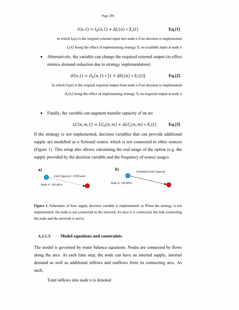
Page 280
, , ∆ ∗ Eq.[1]
In which I0(n) is the original external input into node n if no decision is implemented
being the effect of implementing strategy Xi on available input at node n
Alternatively, the variable can change the required external output (in effect
mimics demand reduction due to strategy implementation)
, , ∗ 1 ∗ Eq.[2]
In which O0(n) is the original required output from node n if no decision is implemented
being the effect of implementing strategy Xi on required output at node n
Finally, the variable can augment transfer capacity of an arc
, , , , ∗ Eq.[3]
If the strategy is not implemented, decision variables that can provide additional
supply are modelled as a fictional source which is not connected to other sources
(Figure 1). This setup also allows calculating the real usage of the option (e.g. the
supply provided by the decision variable and the frequency of source usage).
Figure 1. Schematic of how supply decision variable is implemented: a) When the strategy is not
implemented, the node is not connected to the network; b) once it is connected, the link connecting
the node and the network is active
A.1.1.3. Model equations and constraints
The model is governed by water balance equations. Nodes are connected by flows
along the arcs. At each time step, the node can have an internal supply, internal
demand as well as additional inflows and outflows from its connecting arcs. As
such,
Total inflows into node n is denoted
Link Capacity= 0 Ml/week
Node A: 140 Ml/w
Unlimited Link Capacity
Node A: 140 Ml/w
a) b)
Page 281
, , ,
Eq.[4]
Total outflows from node n is
, , ,
Eq.[5]
At each non-reservoir node, the following flows conservation equation
applies
, , , ,
Eq.[6]
Deficit, if any, is calculated as
, , ,
Eq.[7]
A node cannot supply more than what is available, nor should it get more
water than its need. Moreover, flows are restricted by available transfer
capacities of the arcs. Subsequently, supply, demand and flows at node n is
subject to constraints as follows
, , Eq.[8]
, , Eq.[9]
, , , , Eq.[10]
At a reservoir node, the node has additional storage capacity and the
ResState variable reflects that changing in storage as follows.
, 0
Eq.[11]
Page 282
,
, 1 ,
, ,
Eq.[12]
The node is subject to constraints as follow
,
∗,
100
Eq.[13]
In which minLevel(n,t) is the minimum reservoir fill (%) as required by the reservoir control
curve
The reservoir cannot store more than its capacity (which is the reservoir
total capacity minus its dead volume)
,
Eq.[14]
A.1.1.4. Constraints on decision variables
Once implemented, the permanent decision cannot be reverted
1 Eq.[15]
A.1.2. PREFERENTIAL MODEL AND MULTICRITERIA ANALYSIS
UNDER UNCERTAINTY
A.1.2.1. Technical background
The core model is capable of generating one or many feasible solutions, which
satisfy all specified constraints. Often, decision makers need to select one solution
out of the feasible solution set X. This selection is based on the user’s criteria set
Rn with n being the number of criteria. Hence, each feasible solution will have an
associating vector q(x) that contains the corresponding values of each criterion. A
solution is weakly Pareto-optimal if no other feasible solution has better values of
all criteria. Mathematically, for our minimization problem (deficit in environmental
Page 283
flows, operating cost and supply-demand deficit), a solution is weakly Pareto-
optimal if
∀ :∃ ∈ 1, . . Eq.[16]
Consequently, a Pareto-optimal solution, or an efficient solution, is defined as
∀ 1. .
∃ ∈ 1, . .
Eq.[17]
The aspiration-reservation based decision support method is mainly based on the
set of Pareto optimal points P (or the Pareto frontier). In essence, the method
defines a utopia point qU that contains the best values of each criterion (e.g.
max | ∈ ) and a nadir point qN that contains the worst values of
each criterion (e.g. min | ∈ ). The users can also specify their
preference by identifying an aspiration point , the desired value set of criteria,
and a reservation point , the lower bound of acceptable criterion values. [For a
problem of three minimized criteria, the Pareto front becomes a surface. Include
illustrative figure here]. In this way, the decision makers can specify a range of
criteria values that they are satisfied with. Aspiration-led decision support strives to
find a Pareto-optimal point that is at the specified aspiration level, if attainable, and
closest to the aspiration level if otherwise. In addition, the user can interactively
change their aspiration level to further explore the Pareto-optimal solution under
that specific setting. With each change in aspiration level, the model obtains a new
Pareto-optimal solution by minimizing an achievement scalarising function
, , .
, , max
Eq.[18]
With ∈ being a criteria vector
∈ being an aspiration point
0 being scaling coeffiecients
being a given small positive number, set to 10-4
Page 284
The methodology employed in this study utilizes a modified version of this
achievement scalarising function, as used in Makowski (1994). In essence, strictly
monotone functions ui(.), termed component achievement functions, are introduced
into the achievement scalarising function as follows
, , min , , , ,
Eq.[19]
For minimization problem, Wierzbicki(1986) defines the function ui as
, ,
1,1,
,
Eq.[20]
With
, being given parameters
(Makowski, 1994)Makowski (1994) uses a piece-wise linear, strictly monotone
function that is interactively defined by the user via their specification of the
aspiration and reservation levels ( , ui of which are assigned a value of 1
and 0, respectively. If only the aspiration and reservation are indicated, the
corresponding weight for criterion i to be used in Eq.21 is
1
Eq.[21]
The user may also give additional information on their preference by indicating
extra ui value for other values of criterion i. Therefore, if the component
achievement function of the i-th criterion has pi segments, the function defining ui
in segment ∈ 1, will take the form
, ,
Eq.[22]
given that
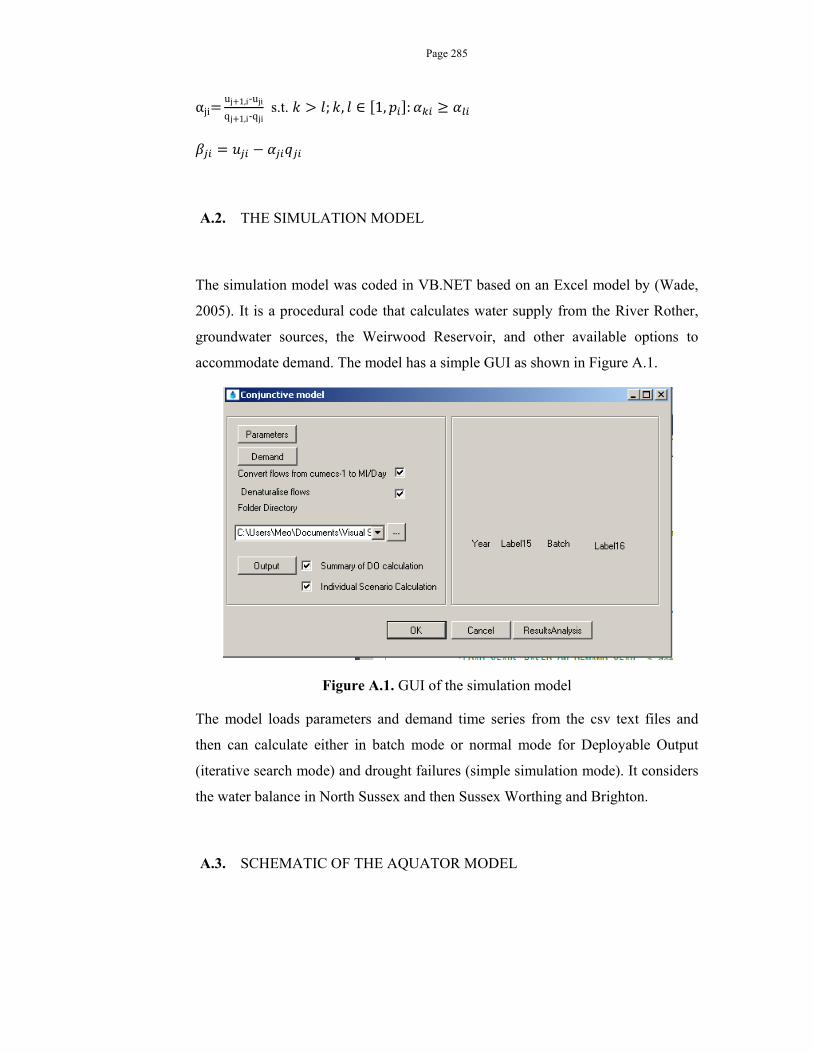
Page 285
αjiuj 1,i‐ujiqj 1,i‐qji
s.t. ; , ∈ 1, :
A.2. THE SIMULATION MODEL
The simulation model was coded in VB.NET based on an Excel model by (Wade,
2005). It is a procedural code that calculates water supply from the River Rother,
groundwater sources, the Weirwood Reservoir, and other available options to
accommodate demand. The model has a simple GUI as shown in Figure A.1.
Figure A.1. GUI of the simulation model
The model loads parameters and demand time series from the csv text files and
then can calculate either in batch mode or normal mode for Deployable Output
(iterative search mode) and drought failures (simple simulation mode). It considers
the water balance in North Sussex and then Sussex Worthing and Brighton.
A.3. SCHEMATIC OF THE AQUATOR MODEL
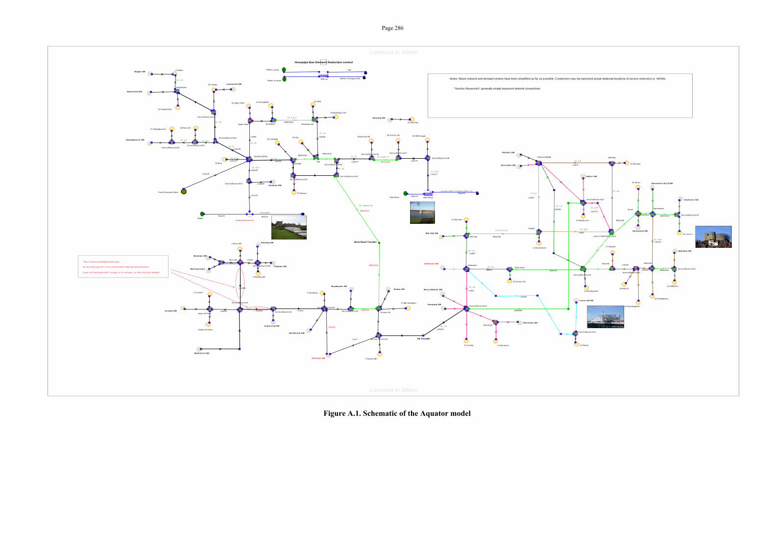
Page 286
Figure A.1. Schematic of the Aquator model
Licenced to Atkins
Licenced to Atkins
FL: 5 & -5
FL: 6.7 & -4.3
FL: 7.9
FL: 9.7
FL: 4.4
FL: 10.2
FL: 8.6
FL: 4.6
FL: 5.5
FL: 21.6FL: 7.4
FL: 10.5
FL: 7.0
Notes: Mains network and demand centres have been simplified as far as possible. Connectors may not represent actual relational locations of service reservoirs or WSWs.
"Service Reservoirs" generally simply represent network connections
FL: 32
FL: 2.7 FL: 62
FL: 25
FL: 9
FL: 4.5FL: 2.5
FL: 2.4
64.36 MRF
FL: 15 and -15
FL: 32 FL: 9 and -17
FL: 21.8
FL: 4.5
FL: 14
FL: 73.5
Summer MRF: 5.5 Winter MRF: 3.5
Hosepipe Ban Demand Reduction control
V6 Transfer
Rock Road Transfer
These 2 links are potentially bi-directional,
Create as bi-directional Links if outages or, for schemes, eg. ASR, need to be modelled
but not used to go north / w est w hen Burpham / Warning Camp operational.
1 Arundel+
2 Batw orth Park+
Arundel GW
Madehurst GW
Link16
3 Perry Hill+
Warning Camp
Burpham GW
Perry Hill
Angmering GW
4 Patching Hill
Link20
Clapham GW
ServiceReservoir3
ServiceReservoir4
5 Worthing+
Northbrook GW
6 High Salvington
Stanhope GW
Broadw ater GW
7 Tenants Hill+
Findon GW
ServiceReservoir5
Link37
Tenants HillBiDiLink3
Service Reservoir9
8 Lancing+
ServiceReservoir10
Link51
Link53
Link55
Shoreham GW
Sompting GW
Shoreham
9 Shoreham+
Mossy Bottom GW
Goldstone GWGoldstone
10 Onslow Rd
Dyke Road
Link67
BiDiLink5
11 Bevendean+
12 Mile Oak+
Mile Oak GW
13 Islingw ord+
Mile Oak
Redhill
BiDiLink6
Patcham GW
Surrenden GW
Patcham Middle
ServiceReservoir10
Link78
Link81
Falmer GW
14 Ditchling Rd+
ServiceReservoir18
Lew es-FalmerWBSs/U13
BiDiLink7
15 Ditchling
Ditchling
BiDiLink9
Link94
16 Marina
ServiceReservoir21
Lew es Rd GW
17 Racehill
Link108
Link110
Racehill
18 Warren
19 Woodingdean+
Balsdean
20 Rottingdean+
ServiceReservoir25
21 Saltdean+
Balsdean GW
BiDiLink12
From Portsmouh Water
22 Sw an
Sw an
New market B,C,D GW
New market
BiDiLink13
Southover GW
24 Lew es+
ServiceReservoir29BiDiLink14
Link128
Batw orth Park
Link129
BiDiLink16
Housedean GW
25 Bury
Hardham WSW
Link133
Hardham GWLink134
Reach1
Link135
Hardham abstraction
Link139
27 Haslingbourne+
ServiceReservoir34
ServiceReservoir35
Haslingbourne GW
Lodsw orth GW28 Vinings
ServiceReservoir36
RotherReach2
29 Petw orth
Knightsf ield
Rotherfield GW
30 Knightsf ield+
Rogate GW31 Rake+
32 Upper Nash
Beedingw ood
33 SWS
34 Beedingw ood+
Star
35 Star
Link159
36 Colstaple
Colstable
37 Wiston+
ServiceReservoir43
ServiceReservoir44
ServiceReservoir45
BiDiLink19BiDiLink20
ServiceReservoir46
38 Buchan Hill
ServiceReservoir47
39 Turners Hill
ServiceReservoir48
40 SEW Supply
Link171
S
Weir WoodWW inflowReach4
Reach5
Link173Link177
Link179Link181
Link184
BiDiLink24Upper Nash
Link190
BiDiLink25
ServiceReservoir50
Link192
41 Itchingf ield+
Itchingf ield
ServiceReservoir52
42 Steyning
Steyning GW
Patching GW
BiDiLink26
ServiceReservoir53
Link197
SC
HPB res
HPBres_topup
Rother In Series
spill
Rother Average prof ile
ServiceReservoir55
Link199
Link201
ServiceReservoir56ServiceReservoir57
Link206
Link207

Page 287
Table B.1. List of link capacity in the Optimisation Model
Parameter Lcap(m,n)/
$ondelim
HardhamWSW UpperValley 63
HardhamWSW Sussex2 175
HardhamWSW Sussex4 434
HardhamWSW Bury 18.9
Portsmouth HardhamWSW 99999
UpperValleyGW UpperValley 99999
HardhamGW Sres53 99999
Sres53 HardhamWSW 514.5
Rother Sres53 99999
Sussex4 BuchanHill 224
Sussex4 TenantsHill 105
TenantsHill Sussex4 105
Sussex2 Sussex3 35
Sussex3 Sussex2 35
Sussex4 Sussex3 98
BuchanHill TurnersHill 119
TurnersHill BuchanHill 63
SEW TurnersHill 99999
Weirwood SEW 152.6
Weirwood MRFWW 99999
Rother MRFRother 99999
TenantsHill BrightonDem1 49
BrightonGW1 BrightonDem1 99999
ShorehamGW Shoreham 99999
ShorehamGW BrightonDem1 99999
BrightonDem2 BrightonDem1 99999
BrightonGW2 BrightonDem2 99999
DesalNode1 ShorehamGW 99999
DesalNode2 ShorehamGW 99999
Arun Sres53 99999
HardhamWSW1 HardhamWSW 99999
HardhamWSW HardhamWSW1 99999
Appendix B-Model Parameters

Page 288
HardhamWSW1 Sussex4 0.0000001
Wellfield Sres53 99999
ASR TenantsHill 99999
Ford Sres53 99999
WorthingGW2 TenantsHill 99999
TenantsHill WorthingDem 99999
WorthingGW1 WorthingDem 99999
$offdelim
/;
Table B.2. Cost Supply in the Optimisation and the Simulation Model
Parameter costSupply(n) / $ondelim BrightonGW1 50 BrightonGW2 50 ShorehamGW 50 HardhamGW 81 Portsmouth 250 Rother 45 UpperValleyGW 50 Weirwood 80 WorthingGW1 50 WorthingGW2 50 $offdelim /;
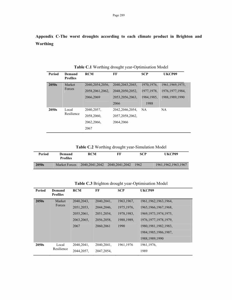
Page 289
Appendix C-The worst droughts according to each climate product in Brighton and
Worthing
Table C.1 Worthing drought year-Optimisation Model
Period Demand Profiles
RCM FF SCP UKCP09
2050s Market Forces
2040,2054,2056,
2058,2061,2062,
2066,2069
2040,2043,2045,
2048,2050,2052,
2053,2056,2063,
2066
1970,1976,
1977,1978,
1984,1985,
1988
1961,1969,1975,
1976,1977,1984,
1988,1989,1990
2050s Local Resilience
2040,2057,
2058,2060,
2062,2066,
2067
2042,2046,2054,
2057,2058,2062,
2064,2066
NA NA
Table C.2 Worthing drought year-Simulation Model
Period Demand Profiles
RCM FF SCP UKCP09
2050s Market Forces 2040,2041,2042 2040,2041,2042 1962 1961,1962,1963,1967
Table C.3 Brighton drought year-Optimisation Model
Period Demand Profiles
RCM FF SCP UKCP09
2050s Market Forces
2040,2043,
2051,2053,
2055,2061,
2063,2065,
2067
2040,2041,
2044,2046,
2051,2054,
2056,2058,
2060,2061
1963,1967,
1975,1976,
1978,1983,
1988,1989,
1990
1961,1962,1963,1964,
1965,1966,1967,1968,
1969,1973,1974,1975,
1976,1977,1978,1979,
1980,1981,1982,1983,
1984,1985,1986,1987,
1988,1989,1990
2050s Local Resilience
2040,2041,
2044,2057,
2040,2041,
2047,2054,
1961,1976 1961,1976,
1989

Page 290
2060,2066,
2067
2057,2058,
2065,2067,
2068
Table C.4 Brighton drought year-Simulation Model
Period Demand Profiles
RCM FF SCP UKCP09
2050s Market Forces
2040 2040 1962 1962
2050s Local Resilience
2040 2040 1961 1961
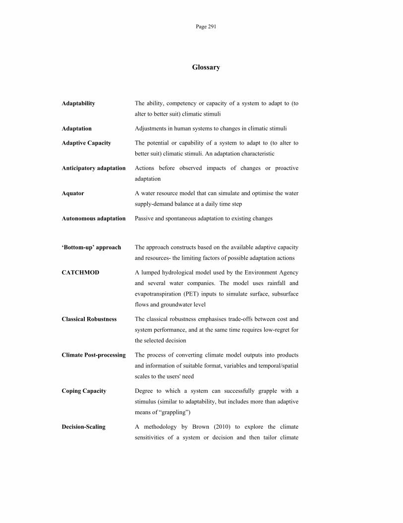
Page 291
Glossary
Adaptability The ability, competency or capacity of a system to adapt to (to
alter to better suit) climatic stimuli
Adaptation Adjustments in human systems to changes in climatic stimuli
Adaptive Capacity The potential or capability of a system to adapt to (to alter to
better suit) climatic stimuli. An adaptation characteristic
Anticipatory adaptation Actions before observed impacts of changes or proactive
adaptation
Aquator A water resource model that can simulate and optimise the water
supply-demand balance at a daily time step
Autonomous adaptation Passive and spontaneous adaptation to existing changes
‘Bottom-up’ approach The approach constructs based on the available adaptive capacity
and resources- the limiting factors of possible adaptation actions
CATCHMOD A lumped hydrological model used by the Environment Agency
and several water companies. The model uses rainfall and
evapotranspiration (PET) inputs to simulate surface, subsurface
flows and groundwater level
Classical Robustness The classical robustness emphasises trade-offs between cost and
system performance, and at the same time requires low-regret for
the selected decision
Climate Post-processing The process of converting climate model outputs into products
and information of suitable format, variables and temporal/spatial
scales to the users' need
Coping Capacity Degree to which a system can successfully grapple with a
stimulus (similar to adaptability, but includes more than adaptive
means of “grappling”)
Decision-Scaling A methodology by Brown (2010) to explore the climate
sensitivities of a system or decision and then tailor climate
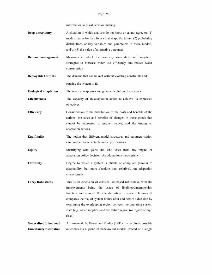
Page 292
information to assist decision making
Deep uncertainty A situation in which analysts do not know or cannot agree on (1)
models that relate key forces that shape the future, (2) probability
distributions of key variables and parameters in these models,
and/or (3) the value of alternative outcomes
Demand management Measures in which the company uses short and long-term
strategies to increase water use efficiency and reduce water
consumption
Deployable Outputs The demand that can be met without violating constraints and
causing the system to fail
Ecological adaptation The reactive responses and genetic evolution of a species
Effectiveness The capacity of an adaptation action to achieve its expressed
objectives
Efficiency Consideration of the distribution of the costs and benefits of the
actions; the costs and benefits of changes in those goods that
cannot be expressed in market values; and the timing on
adaptation actions
Equifinality The notion that different model structures and parameterisation
can produce an acceptable model performance
Equity Identifying who gains and who loses from any impact or
adaptation policy decision. An adaptation characteristic
Flexibility Degree to which a system is pliable or compliant (similar to
adaptability, but more absolute than relative). An adaptation
characteristic
Fuzzy Robustness This is an extension of classical set-based robustness, with the
improvements being the usage of likelihood/membership
function and a more flexible definition of system failures. It
compares the risk of system failure after and before a decision by
examining the overlapping region between the operating system
state (e.g. water supplies) and the failure region (or region of high
risks)
Generalised Likelihood
Uncertainty Estimation
A framework by Beven and Binley (1992) that explores possible
outcomes via a group of behavioural models instead of a single
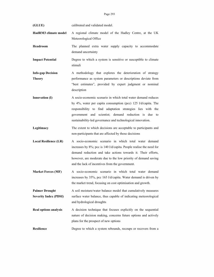
Page 293
(GLUE) calibrated and validated model.
HadRM3 climate model A regional climate model of the Hadley Centre, at the UK
Meteorological Office
Headroom The planned extra water supply capacity to accommodate
demand uncertainty
Impact Potential Degree to which a system is sensitive or susceptible to climate
stimuli
Info-gap Decision
Theory
A methodology that explores the deterioration of strategy
performance as system parameters or descriptions deviate from
“best estimates”, provided by expert judgment or nominal
description
Innovation (I) A socio-economic scenario in which total water demand reduces
by 4%, water per capita consumption (pcc) 125 l/d/capita. The
responsibility to find adaptation strategies lies with the
government and scientist; demand reduction is due to
sustainability-led governance and technological innovation.
Legitimacy The extent to which decisions are acceptable to participants and
non-participants that are affected by those decisions
Local Resilience (LR) A socio-economic scenario in which total water demand
increases by 8%; pcc is 140 l/d/capita. People realise the need for
demand reduction and take actions towards it. Their efforts,
however, are moderate due to the low priority of demand saving
and the lack of incentives from the government.
Market Forces (MF) A socio-economic scenario in which total water demand
increases by 35%, pcc 165 l/d/capita. Water demand is driven by
the market trend, focusing on cost optimisation and growth.
Palmer Drought
Severity Index (PDSI)
A soil moisture/water balance model that cumulatively measures
surface water balance, thus capable of indicating meteorological
and hydrological droughts
Real options analysis A decision technique that focuses explicitly on the sequential
nature of decision making, concerns future options and actively
plans for the prospect of new options
Resilience Degree to which a system rebounds, recoups or recovers from a
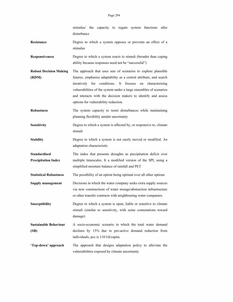
Page 294
stimulus/ the capacity to regain system functions after
disturbance
Resistance Degree to which a system opposes or prevents an effect of a
stimulus
Responsiveness Degree to which a system reacts to stimuli (broader than coping
ability because responses need not be “successful”)
Robust Decision Making
(RDM)
The approach that uses sets of scenarios to explore plausible
futures, emphasise adaptability as a central attribute, and search
iteratively for conditions. It focuses on characterising
vulnerabilities of the system under a large ensembles of scenarios
and interacts with the decision makers to identify and assess
options for vulnerability reduction.
Robustness The system capacity to resist disturbances while maintaining
planning flexibility amidst uncertainty
Sensitivity Degree to which a system is affected by, or responsive to, climate
stimuli
Stability Degree to which a system is not easily moved or modified. An
adaptation characteristic
Standardised
Precipitation Index
The index that presents droughts as precipitation deficit over
multiple timescales. It a modified version of the SPI, using a
simplified moisture balance of rainfall and PET
Statistical Robustness The possibility of an option being optimal over all other options
Supply management Decisions in which the water company seeks extra supply sources
via new constructions of water storage/abstraction infrastructure
or other transfer contracts with neighbouring water companies.
Susceptibility Degree to which a system is open, liable or sensitive to climate
stimuli (similar to sensitivity, with some connotations toward
damage)
Sustainable Behaviour
(SB)
A socio-economic scenario in which the total water demand
declines by 15% due to pro-active demand reduction from
individuals; pcc is 110 l/d/capita.
‘Top-down’ approach The approach that designs adaptation policy to alleviate the
vulnerabilities exposed by climate uncertainty

Page 295
Unsatisfactory State The state occurs when the system displays characteristics outside
of the decision makers’ desired range
Vulnerability Degree to which a system is susceptible to injury, damage, or
harm
Water Resource
Management Plan
The 5-yearly water resource management plan on a 25-year
horizon produced by water companies in England and Wales