Acoustical Measurement of Nonlinear Internal Waves … · Acoustical Measurement of Nonlinear Internal Waves Using the Inverted Echo Sounder QIANG LI AND DAVID M. FARMER Graduate

Acoustical Measurement of Nonlinear Internal Waves Using the InvertedEcho Sounder

QIANG LI AND DAVID M. FARMER

Graduate School of Oceanography, University of Rhode Island, Narragansett, Rhode Island

TIMOTHY F. DUDA

Woods Hole Oceanographic Institution, Woods Hole, Massachusetts

STEVE RAMP

Graduate School of Engineering and Applied Sciences, Naval Postgraduate School, Monterey, California

(Manuscript received 3 July 2008, in final form 5 May 2009)

ABSTRACT

The performance of pressure sensor–equipped inverted echo sounders for monitoring nonlinear internal

waves is examined. The inverted echo sounder measures the round-trip acoustic travel time from the sea floor

to the sea surface and thus acquires vertically integrated information on the thermal structure, from which the

first baroclinic mode of thermocline motion may be inferred. This application of the technology differs from

previous uses in that the wave period (;30 min) is short, requiring a more rapid transmission rate and a

different approach to the analysis. Sources of error affecting instrument performance include tidal effects,

barotropic adjustment to internal waves, ambient acoustic noise, and sea surface roughness. The latter two

effects are explored with a simulation that includes surface wave reconstruction, acoustic scattering based on

the Kirchhoff approximation, wind-generated noise, sound propagation, and the instrument’s signal pro-

cessing circuitry. Bias is introduced as a function of wind speed, but the simulation provides a basis for bias

correction.

The assumption that the waves do not significantly affect the mean stratification allows for a focus on the

dynamic response. Model calculations are compared with observations in the South China Sea by using

nearby temperature measurements to provide a test of instrument performance. After applying corrections

for ambient noise and surface roughness effects, the inverted echo sounder exhibits an RMS variability of

approximately 4 m in the estimated depth of the eigenfunction maximum in the wind speed range 0 # U10 #

10 m s21. This uncertainty may be compared with isopycnal excursions for nonlinear internal waves of 100 m,

showing that the observational approach is effective for measurements of nonlinear internal waves in this

environment.

1. Introduction

Nonlinear internal waves (NLIWs) are widely ob-

served in the ocean, especially in coastal waters (Apel

et al. 2007; Jackson 2007). Among other properties that

have attracted attention over the years is their charac-

teristic shape, which is often associated with a balance

between nonlinearity and dispersion, allowing NLIWs

to propagate great distances with nearly constant char-

acteristics. Recent interest in these waves is motivated

by their roles in energy dissipation and mixing, coastal

biological activities, sediment resuspension, offshore en-

gineering, and underwater acoustics (Duda and Farmer

1998; Apel et al. 2007). The physics of generation and

propagation have been reviewed by several authors

(Apel et al. 2007; Helfrich and Melville 2006), although

many aspects remain poorly understood, motivating de-

velopment of improved observational techniques. The

pressure sensor–equipped inverted echo sounder (PIES)

is a relatively inexpensive and easily deployed instru-

ment that has the potential for effective measurement of

nonlinear internal waves. The concept of inverted echo

Corresponding author address: David M. Farmer, 215 S. Ferry

Rd., Narragansett, RI 02882.

E-mail: [email protected]

2228 J O U R N A L O F A T M O S P H E R I C A N D O C E A N I C T E C H N O L O G Y VOLUME 26

DOI: 10.1175/2009JTECHO652.1

� 2009 American Meteorological Society

Report Documentation Page Form ApprovedOMB No. 0704-0188

Public reporting burden for the collection of information is estimated to average 1 hour per response, including the time for reviewing instructions, searching existing data sources, gathering andmaintaining the data needed, and completing and reviewing the collection of information. Send comments regarding this burden estimate or any other aspect of this collection of information,including suggestions for reducing this burden, to Washington Headquarters Services, Directorate for Information Operations and Reports, 1215 Jefferson Davis Highway, Suite 1204, ArlingtonVA 22202-4302. Respondents should be aware that notwithstanding any other provision of law, no person shall be subject to a penalty for failing to comply with a collection of information if itdoes not display a currently valid OMB control number.

1. REPORT DATE 2009 2. REPORT TYPE

3. DATES COVERED 00-00-2009 to 00-00-2009

4. TITLE AND SUBTITLE Acoustical Measurement of Nonlinear Internal Waves Using the InvertedEcho Sounder

5a. CONTRACT NUMBER

5b. GRANT NUMBER

5c. PROGRAM ELEMENT NUMBER

6. AUTHOR(S) 5d. PROJECT NUMBER

5e. TASK NUMBER

5f. WORK UNIT NUMBER

7. PERFORMING ORGANIZATION NAME(S) AND ADDRESS(ES) Graduate School of Oceanography,University of Rhode Island,Narragansett,RI

8. PERFORMING ORGANIZATIONREPORT NUMBER

9. SPONSORING/MONITORING AGENCY NAME(S) AND ADDRESS(ES) 10. SPONSOR/MONITOR’S ACRONYM(S)

11. SPONSOR/MONITOR’S REPORT NUMBER(S)

12. DISTRIBUTION/AVAILABILITY STATEMENT Approved for public release; distribution unlimited

13. SUPPLEMENTARY NOTES

14. ABSTRACT

15. SUBJECT TERMS

16. SECURITY CLASSIFICATION OF: 17. LIMITATION OF ABSTRACT Same as

Report (SAR)

18. NUMBEROF PAGES

16

19a. NAME OFRESPONSIBLE PERSON

a. REPORT unclassified

b. ABSTRACT unclassified

c. THIS PAGE unclassified

Standard Form 298 (Rev. 8-98) Prescribed by ANSI Std Z39-18

sounders was first developed by Rossby (1969), who

showed that the vertical round-trip travel time of an

acoustic pulse allowed measurement of the variation of

thermal stratification caused by internal tides. They have

been deployed in many areas to study such diverse oce-

anic phenomena as planetary waves, mesoscale eddies,

and large-scale circulation (Watts et al. 2001). Here, we

explore the performance of the instrument, especially

for the study of nonlinear internal waves, using a com-

bination of direct comparisons and model analysis to

reveal the potential and limitations of this measurement

approach.

The acoustic travel time t measured by the inverted

echo sounder is related to the sound speed profile:

t 5 2 3

ð�j

�H

dz

c(z)1 « 5 2 3

ð0

�H

dz

c(z)1 2

�j

c(0)1 «, (1)

where c(z) is the vertical sound speed profile, �j repre-

sents the sea surface elevation caused by low-frequency

barotropic motion such as the tides, H is the instrument

depth, and « represents fluctuations in measured travel

times resulting from variability in scattering of the

acoustic signal by a rough sea surface and effects resulting

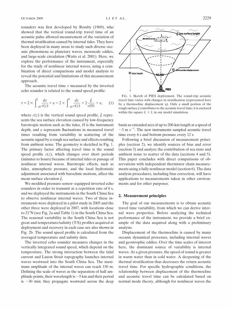
from ambient noise. The geometry is sketched in Fig. 1.

The primary factor affecting travel time is the sound

speed profile c(z), which changes over short periods

(minutes to hours) because of internal tides or passage of

nonlinear internal waves. Barotropic effects, such as

tides, atmospheric pressure, and the local hydrostatic

adjustment associated with baroclinic motions, affect the

mean surface elevation �j.

We modified pressure sensor–equipped inverted echo

sounders in order to transmit at a repetition rate of 6 s,

and we deployed the instruments in the South China Sea

to observe nonlinear internal waves. Two of these in-

struments were deployed in a pilot study in 2005 and the

other three were deployed in 2007, with locations close

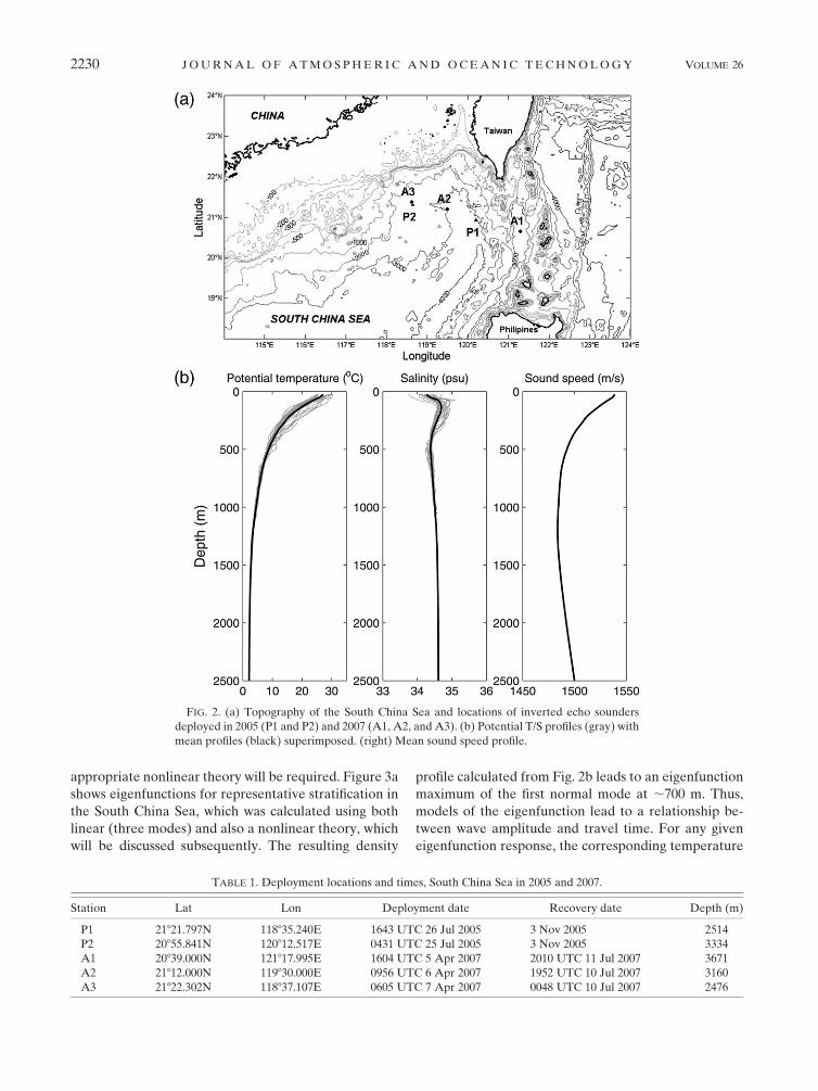
to 218N (see Fig. 2a and Table 1) in the South China Sea.

The seasonal variability in the South China Sea is not

great and temperature/salinity (T/S) profiles acquired at

deployment and recovery in each case are also shown in

Fig. 2b. The sound speed profile is calculated from the

averaged temperature and salinity data.

The inverted echo sounder measures changes in the

vertically integrated sound speed, which depend on the

temperature. The strong interaction between the tidal

current and Luzon Strait topography launches internal

waves westward into the South China Sea. The maxi-

mum amplitude of the internal waves can reach 150 m.

Defining the scale of waves as the separation of half am-

plitude points, their wavelength is ;5 km and their period

is ;30 min; they propagate westward across the deep

basin as extended arcs of up to 200-km length at a speed of

;3 m s21. The new instruments sampled acoustic travel

time every 6 s and bottom pressure every 12 s.

Following a brief discussion of measurement princi-

ples (section 2), we identify sources of bias and error

(section 3) and analyze the contribution of sea state and

ambient noise to scatter of the data (sections 4 and 5).

This paper concludes with direct comparisons of ob-

servations with independent thermistor chain measure-

ments using a fully nonlinear model (section 6). The data

analysis procedures, including bias correction, will have

applications to measurements taken in other environ-

ments and for other purposes.

2. Measurement principles

The goal of our measurements is to obtain acoustic

travel time variability, from which we can derive inter-

nal wave properties. Before analyzing the technical

performance of the instrument, we provide a brief ex-

ample of the data acquired along with a preliminary

analysis.

Displacement of the thermocline is caused by many

oceanic dynamical processes, including internal waves

and geostrophic eddies. Over the time scales of interest

here, the dominant source of variability is internal

waves. At a given pressure, the speed of sound is greater

in warm water than in cold water. A deepening of the

thermal stratification thus decreases the return acoustic

travel time. For specific hydrographic conditions, the

relationship between displacement of the thermocline

and acoustic travel time can be calculated based on

normal mode theory, although for nonlinear waves the

FIG. 1. Sketch of PIES deployment. The round-trip acoustic

travel time varies with changes in stratification (represented here

by a thermocline displacement h). Only a small portion of the

rough surface j contributes to the acoustic travel time; it is enclosed

within the square L 3 L in our model simulation.

OCTOBER 2009 L I E T A L . 2229

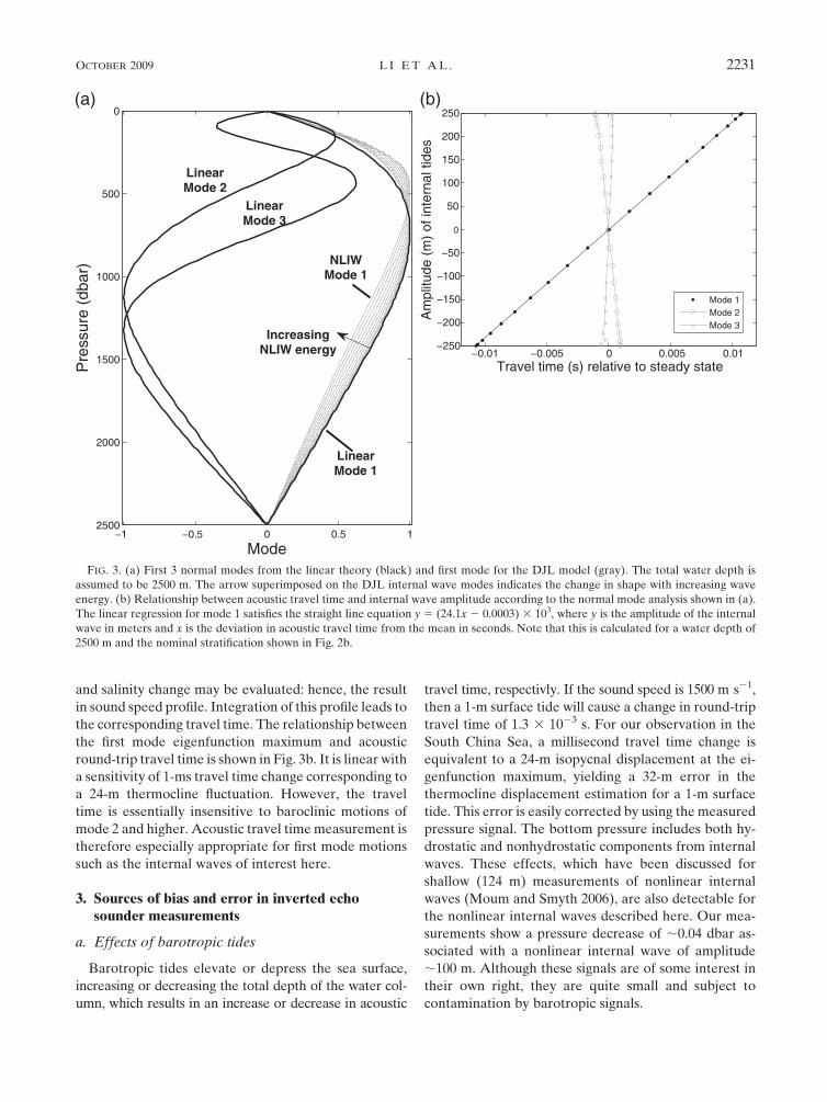
appropriate nonlinear theory will be required. Figure 3a

shows eigenfunctions for representative stratification in

the South China Sea, which was calculated using both

linear (three modes) and also a nonlinear theory, which

will be discussed subsequently. The resulting density

profile calculated from Fig. 2b leads to an eigenfunction

maximum of the first normal mode at ;700 m. Thus,

models of the eigenfunction lead to a relationship be-

tween wave amplitude and travel time. For any given

eigenfunction response, the corresponding temperature

TABLE 1. Deployment locations and times, South China Sea in 2005 and 2007.

Station Lat Lon Deployment date Recovery date Depth (m)

P1 21821.797N 118835.240E 1643 UTC 26 Jul 2005 3 Nov 2005 2514

P2 20855.841N 120812.517E 0431 UTC 25 Jul 2005 3 Nov 2005 3334

A1 20839.000N 121817.995E 1604 UTC 5 Apr 2007 2010 UTC 11 Jul 2007 3671



FIG. 2. (a) Topography of the South China Sea and locations of inverted echo sounders

deployed in 2005 (P1 and P2) and 2007 (A1, A2, and A3). (b) Potential T/S profiles (gray) with

mean profiles (black) superimposed. (right) Mean sound speed profile.


and salinity change may be evaluated: hence, the result

in sound speed profile. Integration of this profile leads to

the corresponding travel time. The relationship between

the first mode eigenfunction maximum and acoustic

round-trip travel time is shown in Fig. 3b. It is linear with

a sensitivity of 1-ms travel time change corresponding to

a 24-m thermocline fluctuation. However, the travel

time is essentially insensitive to baroclinic motions of

mode 2 and higher. Acoustic travel time measurement is

therefore especially appropriate for first mode motions

such as the internal waves of interest here.

3. Sources of bias and error in inverted echosounder measurements

a. Effects of barotropic tides

Barotropic tides elevate or depress the sea surface,

increasing or decreasing the total depth of the water col-

umn, which results in an increase or decrease in acoustic

travel time, respectivly. If the sound speed is 1500 m s21,

then a 1-m surface tide will cause a change in round-trip

travel time of 1.3 3 1023 s. For our observation in the

South China Sea, a millisecond travel time change is

equivalent to a 24-m isopycnal displacement at the ei-

genfunction maximum, yielding a 32-m error in the

thermocline displacement estimation for a 1-m surface

tide. This error is easily corrected by using the measured

pressure signal. The bottom pressure includes both hy-

drostatic and nonhydrostatic components from internal

waves. These effects, which have been discussed for

shallow (124 m) measurements of nonlinear internal

waves (Moum and Smyth 2006), are also detectable for

the nonlinear internal waves described here. Our mea-

surements show a pressure decrease of ;0.04 dbar as-

sociated with a nonlinear internal wave of amplitude

;100 m. Although these signals are of some interest in

their own right, they are quite small and subject to

contamination by barotropic signals.

FIG. 3. (a) First 3 normal modes from the linear theory (black) and first mode for the DJL model (gray). The total water depth is

assumed to be 2500 m. The arrow superimposed on the DJL internal wave modes indicates the change in shape with increasing wave

energy. (b) Relationship between acoustic travel time and internal wave amplitude according to the normal mode analysis shown in (a).

The linear regression for mode 1 satisfies the straight line equation y 5 (24.1x 2 0.0003) 3 103, where y is the amplitude of the internal

wave in meters and x is the deviation in acoustic travel time from the mean in seconds. Note that this is calculated for a water depth of

2500 m and the nominal stratification shown in Fig. 2b.


b. Hydrostatic effects from baroclinic motion(internal tides)

As the thermocline deepens during passage of an in-

ternal wave, the sea surface is elevated to balance the

deceleration. A simple illustration for nonlinear internal

waves is provided by calculating the thermocline dis-

placement h for a wave by using the two-layer Korteweg–

de Vries (KdV) solution:

h(x, t) 5 h0

sech2 x� Vt

D. (2)

The nonlinear velocity V and characteristic width D are

related to the linear wave speed c0 and the amplitude of

the wave h0:

V 5 c0

1ah

0

3and D2 5

12b

ah0

, (3)

where a and b are the nonlinear and dispersion pa-

rameters, respectively, that are determined by the local

stratification. The velocity in the upper layer can be

obtained from the continuity equation with the steady

wave assumption (X 5 x 2 Vt):

u1

5 �V

h1

h. (4)

The surface elevation is then obtained by integrating the

horizontal momentum equation assuming h vanishes at

x / 6‘:

j 5�1

g

ð x

�‘

Du1

Dtdx9 5�1

g

ð j

�‘

(u1� V)

du1

dx9dx9,

5�V2

gh1

1

2

h

h1

1 1

� �h ’ �V2

gh1

h. (5)

Thus, the ratio between the surface elevation and in-

terface depression is ;(V2/gh1), which is primarily de-

termined by the local stratification. This result reduces

to the linear solution j/h 5 Dr/r0 3 h2/(h1 1 h2) if V 5

[Dr/r0 3 gh1h2/(h1 1 h2)]1/2 for h� h1, where h1 and h2

are upper- and lower-layer thicknesses in a two-layer

fluid, Dr is the density difference, and r0 is the mean

density. In the South China Sea, the sea surface eleva-

tion is about 0.18 m for a 100-m thermocline depression

corresponding to a 0.24 3 1023 s increase in travel time.

This is equivalent to the effect of a 6-m isopycnal dis-

placement at the eigenfunction maximum. This modest

(;4%) correction is readily included in calculations of

internal wave properties derived from inverted echo

sounder measurements.

c. Effect of sea state and ambient noise

Additional effects resulting from sea state and ambi-

ent noise are represented by the term « in Eq. (1). From

the measured temperature profiles at station P2, we

found that, in the absence of internal wave packets, the

background internal wave field with period less than

30 min contributes an RMS variability in isotherm dis-

placement maxima of ;3 m. With rising wind speed, the

measurement is simultaneously influenced by the in-

crease in surface roughness and the increase in wind-

generated ambient noise. The joint consequence of these

effects is the primary reason for the scattered distribution

of travel times apparent in Fig. 4. In this section, we seek

to explain this variability. Ambient noise is a passive

variable in this process, which is mainly determined by

wind speed in the frequency band 1–25 kHz (Knudsen

et al. 1948). Acoustic scattering from a rough surface has

been well studied by the acoustic and remote sensing

community. The scattering is determined by the prop-

erties of the acoustic system and by the characteristics of

the rough sea surface. (We note here that effects re-

sulting from advection or refraction of the acoustic pulse

by the current are small. Vertical advection effects are

negligible for the two-way propagation; horizontal shear

effects are governed by the Mach number M ; 1/1500,

and they are also negligible.)

Lord Rayleigh studied the scattering of sound waves

at a sinusoidal boundary (Rayleigh 1877; Beckmann and

Spizzichino 1963; Fortuin 1970). Holford (1981) proposed

an exact solution of the scattering of sound for a sinusoidal

pressure-release surface, although numerical implemen-

tation is difficult. Having solved the problem for a periodic

surface, the result is readily extended to an arbitrary ran-

dom surface via Fourier superposition (Rice 1951). Eckart

(1953) calculated the Helmholtz integral by applying two

boundary conditions: one is the pressure-release surface

and the other is obtained from the method of physical

optics (i.e., the Kirchhoff approximation, which requires

that the normal derivative for the incident and reflected

waves be equal). Clay (1960) compared these theories with

experimental results from Brown and Ricard (1960).

Rayleigh’s method requires the surface slope be suf-

ficiently small. The Kirchhoff approximation is valid

under the restriction that the radius of curvature Rc

obeys the inequality

Rc

$l

p sin3u, (6)

where u is the local grazing angle (i.e., the angle with

respect to the horizon) and l is the wavelength of

the incident waves. To avoid the above restrictions, a

composite-roughness theory was developed (Kur’ynov


1963; McDaniel and Gorman 1983), in which the sea

surface is split into two components: a large-scale and a

small-scale surface, which correspond to the Kirchhoff

and Rayleigh approximations, respectively. McDaniel

(1986) improved this method to reduce dependence on

the scale separation criteria and also showed that, for

large grazing angles (.708), the contribution of the

large-scale surface is dominant. Therefore, for the pre-

sent implementation, the Kirchhoff approximation is

appropriate.

Scattering from resonant subsurface bubbles is an-

other potential source of surface reverberation. The

bubble radius at resonance ar for a 12-kHz acoustic

signal of f 5 12 kHz is ar 5 3.2f 21 5 267 mm. The scat-

tering contribution is determined by bubble density and

distribution, which is also related to the surface wind.

For the acoustic frequency range 3–25 kHz, backscat-

tering at grazing angles above 308 is found to be in

agreement with the predictions of rough surface scat-

tering theory (McDaniel 1993). Very high attenuation

by bubbles can occur sporadically near the surface at

high wind speeds (.10 m s21). Bubbles can also affect

ambient noise. Farmer and Lemon (1984) showed that

at higher frequencies the ocean becomes a quieter place

as the wind increases above about 10 m s21, because the

sound generated by breaking waves is attenuated by

bubble clouds. The effect is modest at 8 kHz but sig-

nificant at 14.5 kHz, which suggests that our 12-kHz

signals will be affected above 10 m s21. At still higher

acoustic frequencies (;100 kHz), bubble densities may

occasionally become so great that they mask the sur-

face from active sonar systems (Farmer et al. 2002) and

show up as increased noise in travel time measurement;

however, at 12 kHz and for wind speeds representative

of most of our data, the primary effect of bubbles is

likely to be to reduce ambient noise in the upper wind

speed range. Bubbles also change the effective sound

speed. However, this is only significant very close to the

sea surface, and it is also intermittent. Taking Terrill and

Melville’s (1997) results as a guide, the effective sound

speed correction of the surface bubble layer at a wind

speed of 10 m s21 will be a maximum, although sporadic,

increase in acoustic travel time of 0.1 ms. This corre-

sponds to an increase of the depth of the eigenfunction

maximum of 2.4 m.

4. Contribution from the sea state

a. Numerical simulation of the transducer

The pressure-equipped inverted echo sounder is

composed of an anchor stand, acoustic release, internal

circuit, and a transducer (ITC-3431C). In the South

China Sea experiment, the instrument was set to trans-

mit an acoustic pulse with a 6 3 1023 s duration. The

carrier frequency of the acoustic pulse is fc 5 12 kHz.

For a nominal sound speed of 1500 m s21 at the source,

the carrier acoustic wavelength is l 5 0.125 m. The

shape of the transducer is a circular piston with radius

a 5 5 cm. In the far field, the acoustic signal can be

computed in cylindrical coordinates (r, u) by the inte-

gration of point sources:

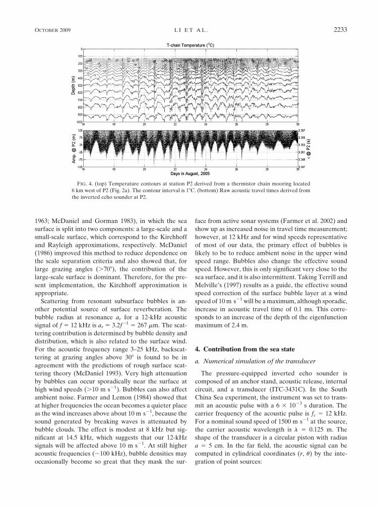
FIG. 4. (top) Temperature contours at station P2 derived from a thermistor chain mooring located

6 km west of P2 (Fig. 2a). The contour interval is 18C. (bottom) Raw acoustic travel times derived from

the inverted echo sounder at P2.


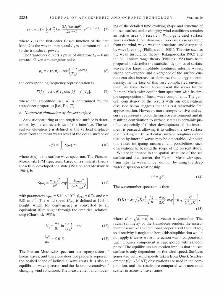
p(r, u, t) 5j

2A

1

a

rka

2J1(ka sinu)

ka sinu

� �ej(2pf

ct�kr), (7)

where J1 is the first-order Bessel function of the first

kind, k is the wavenumber, and A1 is a constant related

to the transducer power.

The transducer directs a pulse of duration T0 5 6 ms

upward. Given a rectangular pulse

p0

5 A(r, u) 3 rectt

T0

� �e j2pf ct, (8)

the corresponding frequency representation is

P( f ) 5 A(r, u)T0

sinc[( f � fc)T

0], (9)

where the amplitude A(r, u) is determined by the

transducer properties [i.e., Eq. (7)].

b. Numerical simulation of the sea surface

Acoustic scattering at the rough sea surface is deter-

mined by the characteristics of the interface. The sea

surface elevation j is defined as the vertical displace-

ment from the mean water level of the ocean surface or

hj2i5ð‘

0

S(v) dv, (10)

where S(v) is the surface wave spectrum. The Pierson–

Moskowitz (PM) spectrum, based on a similarity theory

for a fully developed sea state (Pierson and Moskowitz

1964), is

S(v) 5a

PMg2

v5exp �

bPM

g4

(vU19:5

)4

" #, (11)

with parameters aPM 5 8.10 3 1023, bPM 5 0.74, and g 5

9.81 m s22. The wind speed U19.5 is defined at 19.5-m

height, which for convenience is converted to an

equivalent 10-m height through the empirical relation-

ship (Charnock 1955):

Uz

5u*0.4

lnz

z0

� �and (12)

z0g

u2*

5 0.015. (13)

The Pierson–Moskowitz spectrum is a superposition of

linear waves, and therefore does not properly represent

the peaked shape of individual wave crests. It is also an

equilibrium wave spectrum and thus less representative of

changing wind conditions. The measurement and model-

ing of the detailed time evolving shape and structure of

the sea surface under changing wind conditions remains

an active area of research. Wind-generated surface

waves include three dynamical processes: energy input

from the wind, wave–wave interactions, and dissipation

by wave breaking (Phillips et al. 2001). Theories such as

the weak turbulence theory (Kitaigorodskii 1992) and

the equilibrium range theory (Phillips 1985) have been

proposed to describe the statistical dynamics of surface

waves. For large amplitude nonlinear internal waves,

strong convergence and divergence of the surface cur-

rent can also increase or decrease the energy spectral

density. In the face of this very complicated environ-

ment, we have chosen to represent the waves by the

Pierson–Moskowitz equilibrium spectrum with its sim-

ple superposition of linear wave components. The gen-

eral consistency of the results with our observations

discussed below suggests that this is a reasonable first

approximation. However, more comprehensive and ac-

curate representation of the surface environment and its

resulting contribution to surface scatter is certainly jus-

tified, especially if further development of the instru-

ment is pursued, allowing it to collect the raw surface

scattered signal. In particular, surface roughness mod-

ulation by internal waves may be detectable. Although

this raises intriguing measurement possibilities, such

observations lie beyond the scope of the present study.

We are interested in the spatial structure of the sea

surface and thus convert the Pierson–Moskowitz spec-

trum into the wavenumber domain by using the deep

water dispersion relationship

v2 5 gK. (14)

The wavenumber spectrum is then

W(K) 5 S(ffiffiffiffiffiffiffigK

p)

1

2

ffiffiffiffig

K

r5

aPM

2K3exp �b

PM

g2

U419:5K2

" #,

(15)

where K 5

ffiffiffiffiffiffiffiffiffiffiffiffiffiffiffik2

x 1 k2y

qis the vector wavenumber. The

radial symmetry of the transducer renders the instru-

ment insensitive to directional properties of the surface,

so directivity is neglected here (this simplification would

not apply if wave–wave interaction was incorporated).

Each Fourier component is superposed with random

phase. The equilibrium assumption implies that the sea

surface is only dependent on the wind speed. Surfaces

generated with wind speeds taken from Quick Scatter-

ometer (QuikSCAT) observations are used in the com-

putation, and the results are compared with measured

scatter in acoustic travel times.


c. Numerical simulation of acoustic backscatteringand propagation

The transducer emits a 12-kHz acoustic pulse from the

sea floor (z 5 2H) to the sea surface at z 5 0. For the

purpose of evaluating contributions from ambient noise

and surface roughness, we assume a uniform nominal

sound speed (cs0 5 1500 m s21) in the water column;

specifically, we assume that changes in sound speed

stratification resulting from internal waves are not di-

rectly coupled to the surface scattering problem. When

the sound wave arrives at the sea surface, the amplitude

and phase of the acoustic field can be obtained analyti-

cally, based on the properties of the transducer. Small

incident angle scattering satisfies the Kirchhoff approxi-

mation. With the pressure-release boundary condition,

the sea surface elevation will cause a phase change of the

reflected wave equal to

Du 5 2p2j

l, (16)

with the reflected wave amplitude equal to that of the

incident wave. This phase change is incorporated into

the subsequent acoustic propagation model as the sur-

face boundary condition.

For computational economy, our calculations were

limited to a water depth of H 5 1024 m. Computation

for a depth of 512 m produced essentially the same re-

sults. The instrument threshold is adjusted to detect the

pulse arrival over an initial time step DT 5 3 ms. Thus,

the total duration of the observed signal is much greater

than the short period of useful measurement DT and

allows us to limit the horizontal range of the calculation

domain L accordingly:

L . 2ffiffiffiffiffiffiffiffiffiffiffiffiffiffiffiffiffiffiffiffiffiffiffiffiffiffiffiffiffiffiffiffiffiffiffiffiffiffiffi2c

s0DTH 1 c2

s0DT2q

. (17)

For H 5 1024 m, L . 192 m, the computation domain is

chosen to be 200 m 3 200 m. The grid size of 2048 3 2048

and a vertically integrated step of 4 m are implemented

to control aliasing of the surface. Acoustical signals

propagating beyond this domain are damped. The

transducer is placed in the center of the domain.

Propagation of the acoustic pulse is simulated by using

the parabolic equation (PE). Recently, Duda (2006a,b)

implemented the PE with a wide-angle split-step algo-

rithm (Thomson and Chapman 1983) to study three-

dimensional acoustic propagation. The method relies on

two assumptions: 1) local variations in refractive index

are small and 2) the effective propagation paths are

limited to a narrow aperture. Both requirements are

satisfied in the present application. Given a rotationally

symmetric acoustic field c 5 p(r, z) exp(2jvt) in cylin-

drical coordinates (r, u, z), the pressure resulting from a

point source satisfies the Helmholtz equation

1

r

›

›rr

›p

›r

� �1

›2p

›z21 k2

0n2p 5 0, (18)

where n(r, z) 5 cs0/cs(r, z) is the acoustic refractive in-

dex, which is determined by the ratio of a reference

sound speed cs0 to the sound speed cs of the medium;

k0 5 v/cs0 is the reference wavenumber.

With the transformation

p(r, z) 5u(r, z)ffiffi

rp (19)

and the adoption of two operators

P 5›

›rand Q 5 n2 1 k�2

0

›2

›z2

� �1/2

, (20)

(18) can be transformed into parabolic form

Pu 5 ik0Qu, (21)

which admits numerical solution without iteration. Fi-

nite bandwidth pulses are simulated by using Fourier

synthesis.

d. Estimation of ambient noise and transmission loss

To minimize instrument energy requirements, the

output power of the transducer is set relatively low,

sound pressure level being adjusted from 170 to

200 dB re 1 mPa at 1 m from the transducer, depending

on deployment depth. Ambient noise is closely related

to wind speed in the bandwidth of interest (Knudsen

et al. 1948). The ambient noise level at 12 kHz varies

from 40 to 60 dB re 1 mPa Hz21/2 through the wind speed

range 1–15 m s21 (Wenz 1962). Other unknown noise,

including instrument noise, is estimated to be less than

10 dB re 1 mPa Hz21/2 based on a pilot test. Use of a

narrowband-limited filter in the PIES circuit justifies

representation of the noise by a white Gaussian signal.

The energy loss resulting from scattering and transmis-

sion spreading is given by the PE model. Transmission

loss resulting from absorption is small and ignored

(Urick 1983). We calculate a 10–30-dB difference be-

tween the maximum received pulse level and the noise

level over the wind speed range 1 # U10 # 15 m s21. The

attenuation of 12-kHz noise by bubble clouds at wind

speeds above 10 m s21 was identified in section 3c, but

our data are few and scattered at these wind speeds and

this effect is not explicitly included in the simulation.


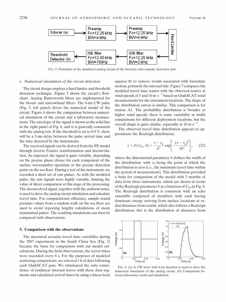
e. Numerical simulation of the circuit detection

The circuit design employs a hard limiter and threshold

detection technique. Figure 5 shows the circuit’s flow-

chart. Analog Butterworth filters are implemented for

the broad- and narrowband filters. The 6-ms CW pulse

(Fig. 5, left panel) drives the numerical model of the

circuit. Figure 6 shows the comparison between numeri-

cal simulation of the circuit and a laboratory measure-

ment. The envelope of the signal is shown as the solid line

in the right panel of Fig. 6, and it is generally consistent

with the analog test. If the threshold is set to 0.9 V, there

will be a 3-ms delay between the pulse arrival time and

the time detected by the instruments.

The received signals can be derived from the PE model

through inverse Fourier transformation and deconvolu-

tion. As expected, the signal is quite variable, depending

on the precise phase choice for each component of the

surface wavenumber spectrum or the precise detection

point on the sea floor. During a test of the instrument, we

recorded a short set of raw pulses. As with the modeled

pulse, the raw signals were highly variable, limiting the

value of direct comparison at this stage of the processing.

The deconvolved signal, together with the ambient noise,

is used to drive the analog circuit simulation and calculate

travel time. For computational efficiency, sample sound

pressure values from a random walk on the sea floor are

used to avoid repeating lengthy calculations of many

transmitted pulses. The resulting simulations can then be

compared with observations.

5. Comparison with the observations

The measured acoustic travel time variability during

the 2007 experiment in the South China Sea (Fig. 2)

became the basis for comparison with our model cal-

culations. During the field observations, the travel times

were recorded every 6 s. For the purposes of modeled

scattering comparisons, we selected 1 h of data following

each QuikSCAT pass. We eliminated the only coinci-

dence of nonlinear internal waves with these data seg-

ments and calculated arrival times by using a linear least

squares fit to remove trends associated with baroclinic

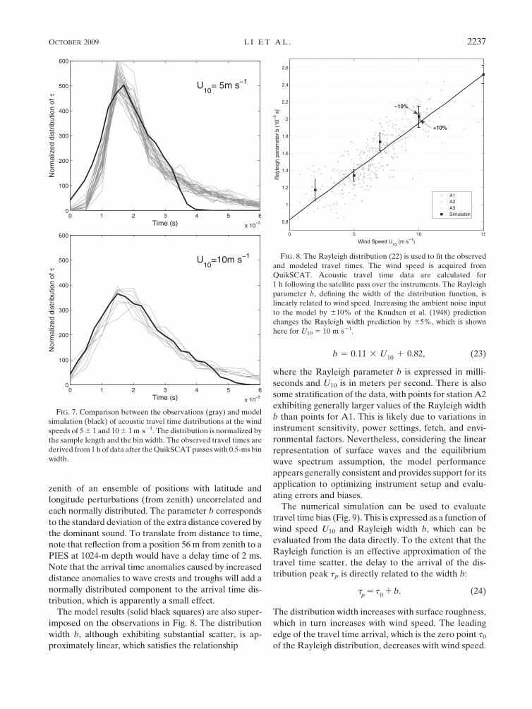
motion, primarily the internal tide. Figure 7 compares the

modeled travel time scatter with the observed scatter at

wind speeds of 5 and 10 m s21 based on QuikSCAT wind

measurements for the instrument locations. The shape of

the distribution curves is similar. This comparison is for

station A1. The probability distribution is broader at

higher wind speeds; there is some variability in width

comparisons for different deployment locations, but the

overall shape is quite similar, especially at 10 m s21.

The observed travel time distribution appears to ap-

proximate the Rayleigh distribution:

y 5 f (tjt0, b) 5

t � t0

b2exp �

(t � t0)2

2b2

" #, (22)

where the dimensional parameter b defines the width of

the distribution, with t0 being the point at which the

distribution is zero (i.e., the minimum travel time within

the period of measurement). This distribution provided

a basis for comparison of the model with 3 months of

data from three instruments, which are shown in terms

of the Rayleigh parameter b as a function of U10 in Fig. 8.

The Rayleigh distribution is consistent with an echo

ensemble composed of members with each having

dominant energy arriving from surface locations at ra-

dial distances from zenith, which also follows a Rayleigh

distribution; this is the distribution of distances from

FIG. 5. Flowchart of the simulated analog circuit of the inverted echo sounder detection unit.

FIG. 6. (a) A CW wave with 6-ms duration is used to drive the

numerical simulation of the analog circuit. (b) Comparison be-

tween laboratory result and simulation.


zenith of an ensemble of positions with latitude and

longitude perturbations (from zenith) uncorrelated and

each normally distributed. The parameter b corresponds

to the standard deviation of the extra distance covered by

the dominant sound. To translate from distance to time,

note that reflection from a position 56 m from zenith to a

PIES at 1024-m depth would have a delay time of 2 ms.

Note that the arrival time anomalies caused by increased

distance anomalies to wave crests and troughs will add a

normally distributed component to the arrival time dis-

tribution, which is apparently a small effect.

The model results (solid black squares) are also super-

imposed on the observations in Fig. 8. The distribution

width b, although exhibiting substantial scatter, is ap-

proximately linear, which satisfies the relationship

b 5 0.11 3 U101 0.82, (23)

where the Rayleigh parameter b is expressed in milli-

seconds and U10 is in meters per second. There is also

some stratification of the data, with points for station A2

exhibiting generally larger values of the Rayleigh width

b than points for A1. This is likely due to variations in

instrument sensitivity, power settings, fetch, and envi-

ronmental factors. Nevertheless, considering the linear

representation of surface waves and the equilibrium

wave spectrum assumption, the model performance

appears generally consistent and provides support for its

application to optimizing instrument setup and evalu-

ating errors and biases.

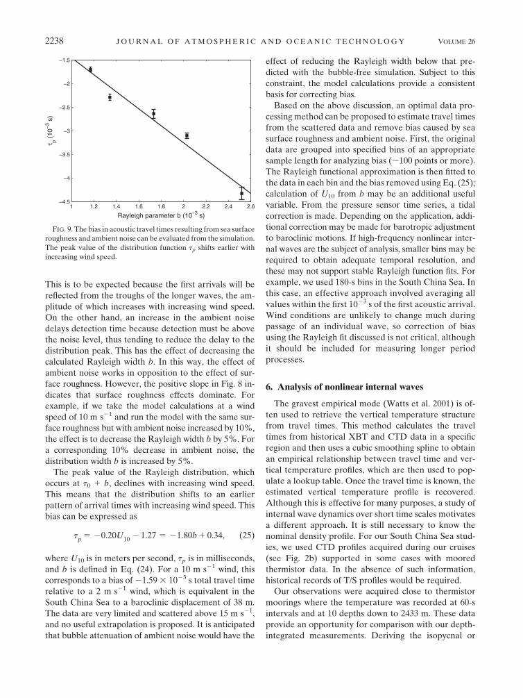
The numerical simulation can be used to evaluate

travel time bias (Fig. 9). This is expressed as a function of

wind speed U10 and Rayleigh width b, which can be

evaluated from the data directly. To the extent that the

Rayleigh function is an effective approximation of the

travel time scatter, the delay to the arrival of the dis-

tribution peak tp is directly related to the width b:

tp

5 t0

1 b. (24)

The distribution width increases with surface roughness,

which in turn increases with wind speed. The leading

edge of the travel time arrival, which is the zero point t0

of the Rayleigh distribution, decreases with wind speed.

FIG. 7. Comparison between the observations (gray) and model

simulation (black) of acoustic travel time distributions at the wind

speeds of 5 6 1 and 10 6 1 m s21. The distribution is normalized by

the sample length and the bin width. The observed travel times are

derived from 1 h of data after the QuikSCAT passes with 0.5-ms bin

width.

FIG. 8. The Rayleigh distribution (22) is used to fit the observed

and modeled travel times. The wind speed is acquired from

QuikSCAT. Acoustic travel time data are calculated for

1 h following the satellite pass over the instruments. The Rayleigh

parameter b, defining the width of the distribution function, is

linearly related to wind speed. Increasing the ambient noise input

to the model by 610% of the Knudsen et al. (1948) prediction

changes the Rayleigh width prediction by 65%, which is shown

here for U10 5 10 m s21.


This is to be expected because the first arrivals will be

reflected from the troughs of the longer waves, the am-

plitude of which increases with increasing wind speed.

On the other hand, an increase in the ambient noise

delays detection time because detection must be above

the noise level, thus tending to reduce the delay to the

distribution peak. This has the effect of decreasing the

calculated Rayleigh width b. In this way, the effect of

ambient noise works in opposition to the effect of sur-

face roughness. However, the positive slope in Fig. 8 in-

dicates that surface roughness effects dominate. For

example, if we take the model calculations at a wind

speed of 10 m s21 and run the model with the same sur-

face roughness but with ambient noise increased by 10%,

the effect is to decrease the Rayleigh width b by 5%. For

a corresponding 10% decrease in ambient noise, the

distribution width b is increased by 5%.

The peak value of the Rayleigh distribution, which

occurs at t0 1 b, declines with increasing wind speed.

This means that the distribution shifts to an earlier

pattern of arrival times with increasing wind speed. This

bias can be expressed as

tp

5 �0.20U10� 1.27 5 �1.80b 1 0.34, (25)

where U10 is in meters per second, tp is in milliseconds,

and b is defined in Eq. (24). For a 10 m s21 wind, this

corresponds to a bias of 21.59 3 1023 s total travel time

relative to a 2 m s21 wind, which is equivalent in the

South China Sea to a baroclinic displacement of 38 m.

The data are very limited and scattered above 15 m s21,

and no useful extrapolation is proposed. It is anticipated

that bubble attenuation of ambient noise would have the

effect of reducing the Rayleigh width below that pre-

dicted with the bubble-free simulation. Subject to this

constraint, the model calculations provide a consistent

basis for correcting bias.

Based on the above discussion, an optimal data pro-

cessing method can be proposed to estimate travel times

from the scattered data and remove bias caused by sea

surface roughness and ambient noise. First, the original

data are grouped into specified bins of an appropriate

sample length for analyzing bias (;100 points or more).

The Rayleigh functional approximation is then fitted to

the data in each bin and the bias removed using Eq. (25);

calculation of U10 from b may be an additional useful

variable. From the pressure sensor time series, a tidal

correction is made. Depending on the application, addi-

tional correction may be made for barotropic adjustment

to baroclinic motions. If high-frequency nonlinear inter-

nal waves are the subject of analysis, smaller bins may be

required to obtain adequate temporal resolution, and

these may not support stable Rayleigh function fits. For

example, we used 180-s bins in the South China Sea. In

this case, an effective approach involved averaging all

values within the first 1023 s of the first acoustic arrival.

Wind conditions are unlikely to change much during

passage of an individual wave, so correction of bias

using the Rayleigh fit discussed is not critical, although

it should be included for measuring longer period

processes.

6. Analysis of nonlinear internal waves

The gravest empirical mode (Watts et al. 2001) is of-

ten used to retrieve the vertical temperature structure

from travel times. This method calculates the travel

times from historical XBT and CTD data in a specific

region and then uses a cubic smoothing spline to obtain

an empirical relationship between travel time and ver-

tical temperature profiles, which are then used to pop-

ulate a lookup table. Once the travel time is known, the

estimated vertical temperature profile is recovered.

Although this is effective for many purposes, a study of

internal wave dynamics over short time scales motivates

a different approach. It is still necessary to know the

nominal density profile. For our South China Sea stud-

ies, we used CTD profiles acquired during our cruises

(see Fig. 2b) supported in some cases with moored

thermistor data. In the absence of such information,

historical records of T/S profiles would be required.

Our observations were acquired close to thermistor

moorings where the temperature was recorded at 60-s

intervals and at 10 depths down to 2433 m. These data

provide an opportunity for comparison with our depth-

integrated measurements. Deriving the isopycnal or

FIG. 9. The bias in acoustic travel times resulting from sea surface

roughness and ambient noise can be evaluated from the simulation.

The peak value of the distribution function tp shifts earlier with

increasing wind speed.


isotherm structure of nonlinear internal waves from

travel times requires an appropriate model. Here, we

illustrate this approach with Long’s (1953) fully non-

linear model, which is based on the Dubriel-Jacotin

(1932) transformation, also called the DJL model. It is

assumed that the lower boundary is a streamline, so

there is no flow separation, that the flow is steady, and

that the conditions far upstream are known (i.e., the

vertical profile of the kinetic energy of the upstreamflow

is known). Under the Dubriel-Jacotin transformation,

the original Boussinesq equations take the form of the

Helmholtz equation (Long 1953; Baines 1995):

=2d 1 k2d 5 0, (26)

where

k2 5N2

U2,(27)

and d(x, z) represents the vertical displacement of the

streamline at (x, z). Also, N and U are the upstream

buoyancy frequency and horizontal velocity, respectively.

The exact solution can be obtained numerically without

restrictions on the degree of nonlinearity or the form of

stratification (Turkington et al. 1991). In contrast to linear

waves, the eigenfunction maximum (Fig. 3) now depends

on amplitude. A corresponding nonlinear eigenvalue or

wave speed is obtained for each wave amplitude.

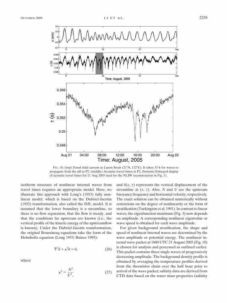
For given background stratification, the shape and

speed of nonlinear internal waves are determined by the

wave amplitude or potential energy. The nonlinear in-

ternal wave packet at 1600 UTC 21 August 2005 (Fig. 10)

is chosen for analysis and processed as outlined earlier.

This packet contains three single waves of progressively

decreasing amplitude. The background density profile is

obtained by averaging the temperature profiles derived

from the thermistor chain over the half hour prior to

arrival of the wave packet; salinity data are derived from

CTD data based on the water mass properties (salinity

FIG. 10. (top) Zonal tidal current at Luzon Strait (218N, 1228E). It takes 33 h for waves to

propagate from the sill to P2. (middle) Acoustic travel times at P2. (bottom) Enlarged display

of acoustic travel times for 21 Aug 2005 used for the NLIW reconstruction in Fig. 11.


variability has a very minor effect on the density profile).

Thus, a lookup table for the nonlinear internal waves

corresponding to a range of different possible energy

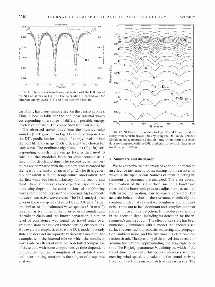
levels is established. The comparison is shown in Fig. 11.

The observed travel times from the inverted echo

sounder (thick gray line in Fig. 11) are superimposed on

the DJL prediction for a range of energy levels to find

the best fit. The energy levels 6, 5, and 4 are chosen for

each wave. The nonlinear eigenfunctions (Fig. 3a) cor-

responding to each fitted energy level is then used to

calculate the modeled isotherm displacement as a

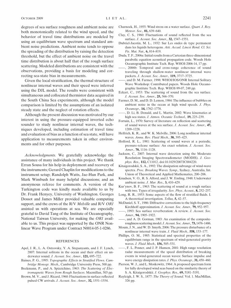
function of depth and time. The reconstructed temper-

atures are compared with the temperatures recorded by

the nearby thermistor chain in Fig. 12. The fit is gener-

ally consistent with the temperature observations for

the first wave but less satisfactory for the second and

third. This discrepancy is to be expected, especially with

increasing depth as the contributions of neighboring

waves combine to increase the isopycnal displacements

between successive wave crests. The DJL analysis also

gives us the wave speeds (3.20, 3.13, and 3.07 m s21) that

are similar to the estimated wave speeds (3.10 m s21)

based on arrival times at the inverted echo sounder and

thermistor chain and the known separation; a similar

level of consistency was found for travel times over

greater distances based on remote sensing observations.

However, it is emphasized that the DJL model is steady

state and does not incorporate variability associated, for

example, with the internal tide on which the nonlinear

waves ride or effects of rotation. A detailed comparison

of these data with more comprehensive time-dependent

models, free of the assumption of an isolated wave

and incorporating rotation, is the subject of a separate

analysis.

7. Summary and discussion

We have shown that the inverted echo sounder can be

an effective instrument for measuring nonlinear internal

waves in the open ocean. Sources of error affecting in-

strument performance are analyzed. The error caused

by elevation of the sea surface, including barotropic

tides and the barotropic pressure adjustment associated

with baroclinic motion, can be easily corrected. The

acoustic behavior due to the sea state, specifically the

combined effect of sea surface roughness and ambient

noise, turns out to be a dominant and complicated error

source in travel time detection. It introduces variability

in the acoustic signal including its detection by the in-

strument’s analog circuit. The effect of sea state has been

numerically simulated with a model that includes sea

surface reconstruction, acoustic scattering and propaga-

tion, ambient noise, and the instrument’s electronic de-

tection circuit. The spreading of the travel time reveals an

asymmetric pattern approximating the Rayleigh func-

tion. The Rayleigh parameter b, defining the width of the

travel time probability distribution, increases with in-

creasing wind speed, equivalent to the sound arriving

from points within a surface patch of increasing size. The

FIG. 11. The acoustic travel times calculated with the DJL model

for NLIWs shown in Fig. 10. The calculation is carried out for

different energy levels (6, 5, and 4) to identify a best fit.

FIG. 12. NLIWs corresponding to Figs. 10 and 11 retrieved di-

rectly from acoustic travel times by using the DJL model (black).

Simultaneous temperature contours (gray) from thermistor chain

data are compared with the DJL predicted isotherm displacements

for the upper 1000 m.


degrees of sea surface roughness and ambient noise are

both monotonically related to the wind speed, and the

behavior of travel time distributions are modeled by

using an equilibrium wave spectrum and standard am-

bient noise predictions. Ambient noise tends to oppose

the spreading of the distribution by raising the detection

threshold, but the effect of ambient noise on the travel

time distribution is about half that of the rough surface

scattering. Modeled distributions are consistent with the

observations, providing a basis for modeling and cor-

recting sea-state bias in measurements.

Given the local stratification, the thermal structure of

nonlinear internal waves and their speed were inferred

using the DJL model. The results were consistent with

simultaneous and collocated thermistor data acquired in

the South China Sea experiments, although the model

comparison is limited by the assumptions of an isolated

steady state and the neglect of rotation effects.

Although the present discussion was motivated by our

interest in using the pressure-equipped inverted echo

sounder to study nonlinear internal waves, the tech-

niques developed, including estimation of travel time

and evaluation of bias as a function of sea state, will have

application to measurements taken in other environ-

ments and for other purposes.

Acknowledgments. We gratefully acknowledge the

assistance of many individuals in this project. We thank

Erran Sousa for his help in deployment and recovery of

the instruments; Gerard Chaplin for modifications to the

instrument setup; Randolph Watts, Jae-Hun Park, and

Mark Wimbush for many helpful discussions; and an

anonymous referee for comments. A version of the

Turkington code was kindly made available to us by

Dr. Frank Henyey, University of Washington. Georges

Dossot and James Miller provided valuable computing

support, and the crews of the R/V Melville and R/V OR1

assisted us with operations at sea. We are especially

grateful to David Tang of the Institute of Oceanography,

National Taiwan University, for making the OR1 avail-

able to us. This project was supported by the ONR Non-

linear Wave Program under Contract N0014-05-1-0286.

REFERENCES

Apel, J. R., L. A. Ostrovsky, Y. A. Stepanyants, and J. F. Lynch,

2007: Internal solitons in the ocean and their effect on un-

derwater sound. J. Acoust. Soc. Amer., 121, 695–722.

Baines, P. G., 1995: Topographic Effects in Stratified Flows. Cam-

bridge Monogr. Mech., Cambridge University Press, 500 pp.

Beckmann, P., and A. Spizzichino, 1963: The Scattering of Elec-

tromagnetic Waves from Rough Surfaces. Macmillan, 503 pp.

Brown, M. V., and J. Ricard, 1960: Fluctuations in surface reflected

pulsed CW arrivals. J. Acoust. Soc. Amer., 32, 1551–1554.

Charnock, H., 1955: Wind stress on a water surface. Quart. J. Roy.

Meteor. Soc., 81, 639–640.

Clay, C. S., 1960: Fluctuations of sound reflected from the sea

surface. J. Acoust. Soc. Amer., 32, 1547–1551.

Dubriel-Jacotin, M. L., 1932: Sur Les ondes de type permanent

dans les liquids heterogens. Atti. Accad. Lincei Rend. Cl. Sci.

Fis. Mat. Nat., 6, 814–819.

Duda, T. F., 2006a: Initial results from a Cartesian three-dimensional

parabolic equation acoustical propagation code. Woods Hole

Oceanographic Institute Tech. Rep. WHOI-2006-14, 17 pp.

——, 2006b: Temporal and cross-range coherence of sound

traveling through shallow-water nonlinear internal wave

packets. J. Acoust. Soc. Amer., 119, 3717–3725.

——, and D. M. Farmer, 1998: WHOI/IOS/ONR Internal Solitary

Wave Workshop: Contributed papers. Woods Hole Oceano-

graphic Institute Tech. Rep. WHOI-99-07, 248 pp.

Eckart, C., 1953: The scattering of sound from the sea surface.

J. Acoust. Soc. Amer., 25, 566–570.

Farmer, D. M., and D. D. Lemon, 1984: The influence of bubbles on

ambient noise in the ocean at high wind speeds. J. Phys.

Oceanogr., 14, 1762–1778.

——, D. Li, B. Donald, and L. Martin, 2002: Wave kinematics at

high sea states. J. Atmos. Oceanic Technol., 19, 225–239.

Fortuin, L., 1970: Survey of literature on reflection and scattering

of sound waves at the sea surface. J. Acoust. Soc. Amer., 47,

1209–1228.

Helfrich, K. R., and W. K. Melville, 2006: Long nonlinear internal

waves. Annu. Rev. Fluid Mech., 38, 395–425.

Holford, R. L., 1981: Scattering of sound waves at a periodic,

pressure-release surface: An exact solution. J. Acoust. Soc.

Amer., 70, 1116–1128.

Jackson, C., 2007: Internal wave detection using the Moderate

Resolution Imaging Spectroradiometer (MODIS). J. Geo-

phys. Res., 112, C11012, doi:10.1029/2007JC004220.

Kitaigorodskii, S. A., 1992: The dissipation subrange of wind-wave

spectra. Proc. Breaking Waves. Symp., Sydney, Australia, Int.

Union of Theoretical and Applied Mathematics, 200–206.

Knudsen, V. O., R. S. Alford, and J. W. Emling, 1948: Underwater

ambient noise. J. Mar. Res., 3, 410–429.

Kur’ynov, B. F., 1963: The scattering of sound at a rough surface

with two. Types of irregularity. Sov. Phys. Acoust., 8, 252–257.

Long, R. R., 1953: Some aspects of the flow of stratified fluids. I.

A theoretical invertigation. Tellus, 5, 42–57.

McDaniel, S. T., 1986: Diffractive corrections to the high-frequency

Kirchhoff approximation. J. Acoust. Soc. Amer., 79, 952–957.

——, 1993: Sea surface reverberation: A review. J. Acoust. Soc.

Amer., 94, 1905–1922.

——, and A. D. Gorman, 1983: An examination of the composite-

roughness scattering model. J. Acoust. Soc. Amer., 73, 1476–1486.

Moum, J. N., and W. D. Smyth, 2006: The pressure disturbance of a

nonlinear internal wave train. J. Fluid Mech., 558, 153–177.

Phillips, O. M., 1985: Statistical and spectral properties of the

equilibrium range in the spectrum of wind-generated gravity

waves. J. Fluid Mech., 156, 505–531.

——, F. L. Posner, and J. P. Hansen, 2001: High range resolution

radar measurements of the speed distribution of breaking

events in wind-generated ocean waves: Surface impulse and

wave energy dissipation rates. J. Phys. Oceanogr., 31, 450–460.

Pierson, W. J., and L. Moskowitz, 1964: A proposed spectrum form

for fully developed wind seas based on the similarity theory of

S. A. Kitaigorodskii. J. Geophys. Res., 69, 5181–5191.

Rayleigh, J. W. S., 1877: The Theory of Sound. Vol. 1. MacMillan,

326 pp.


Rice, S. O., 1951: Reflection of electromagnetic waves from slightly

rough surfaces. Commun. Pure Appl. Math., 4, 351–378.

Rossby, T., 1969: On monitoring depth variations of the main

thermocline acoustically. J. Geophys. Res., 74, 5542–5546.

Terrill, E., and W. K. Melville, 1997: Sound-speed measurements

in the surface-wave layer. J. Acoust. Soc. Amer., 102, 2607–

2625.

Thomson, D. J., and N. R. Chapman, 1983: A wide-angle split-step

algorithm for the parabolic equation. J. Acoust. Soc. Amer., 74,

1848–1854.

Turkington, B., A. Eydeland, and S. Wang, 1991: A computational

method for solitary internal waves in a continuously stratified

fluid. Stud. Appl. Math., 85, 93–127.

Urick, R. J., 1983: Principles of Underwater Sound. McGraw-Hill,

423 pp.

Watts, D. R., C. Sun, and S. Rintoul, 2001: A two-dimensional gravest

empirical mode determined from hydrographic observations in

the Subantarctic Front. J. Phys. Oceanogr., 31, 2186–2209.

Wenz, G. M., 1962: Acoustic ambient noise in the ocean: Spectra

and sources. J. Acoust. Soc. Amer., 34, 1936–1956.


Documents

Acoustical Measurement of Nonlinear Internal Waves … · Acoustical Measurement of Nonlinear Internal Waves Using the Inverted Echo Sounder QIANG LI AND DAVID M. FARMER Graduate