Embed Size (px)
Citation preview
Finance and Economics Discussion SeriesDivisions of Research & Statistics and Monetary Affairs
Federal Reserve Board, Washington, D.C.
Accounting for Productivity Dispersion over the Business Cycle
Robert J. Kurtzman and David Zeke
2016-045
Please cite this paper as:Kurtzman, Robert J., and David Zeke (2016). “Accounting for Productiv-ity Dispersion over the Business Cycle,” Finance and Economics Discussion Se-ries 2016-045. Washington: Board of Governors of the Federal Reserve System,http://dx.doi.org/10.17016/FEDS.2016.045.
NOTE: Staff working papers in the Finance and Economics Discussion Series (FEDS) are preliminarymaterials circulated to stimulate discussion and critical comment. The analysis and conclusions set forthare those of the authors and do not indicate concurrence by other members of the research staff or theBoard of Governors. References in publications to the Finance and Economics Discussion Series (other thanacknowledgement) should be cleared with the author(s) to protect the tentative character of these papers.
Accounting for Productivity Dispersion over theBusiness Cycle ∗
Robert Kurtzman†1 and David Zeke ‡2
1Federal Reserve Board of Governors2University of California, Los Angeles
May 20, 2016
Abstract
This paper presents accounting decompositions of changes in aggregate labor and capitalproductivity. Our simplest decomposition breaks changes in an aggregate productivity ratiointo two components: A mean component, which captures common changes to firm factorproductivity ratios, and a dispersion component, which captures changes in the variance andhigher order moments of their distribution. In standard models with heterogeneous firms andfrictions to firm input decisions, the dispersion component is a function of changes in thesecond and higher moments of the log of marginal revenue factor productivities and reflectschanges in the extent of distortions to firm factor input allocations across firms. We apply ourdecomposition to public firm data from the United States and Japan. We find that the meancomponent is responsible for most of the variation in aggregate productivity over the businesscycle, while the dispersion component plays a modest role.
∗We thank Andy Atkeson, David Baqaee, Brian Cadena, and Pierre-Olivier Weill, and seminar partici-pants at the Spring Midwest Macro Meetings 2015, GCER Conference 2015, WEAI Summer meetings, andEconometric Society World Congress 2015 for their helpful comments and discussions. The views expressedin this paper are solely the responsibility of the authors and should not be interpreted as reflecting the views ofthe Board of Governors of the Federal Reserve System or of anyone else associated with the Federal ReserveSystem.
1 Introduction
What drives changes in aggregate productivity? One explanation that has been widely
used to explain the variation of aggregate productivity over the business cycle or over time
more generally is that frictions to the allocation of labor and capital between firms are time-
varying: Greater frictions to the distribution of capital and labor between firms reduce the
amount of output produced with a given amount of capital and labor and reduce measures
of aggregate productivity.1 This paper presents accounting decompositions of changes in
aggregate labor, capital, and total factor productivity that addresses this economic mecha-
nism, and can help to quantify the extent to which the changing distribution of labor and
capital drive fluctuations in aggregate productivity over time.
The accounting decompositions in this paper rely on the property that aggregate factor
productivity ratios can be expressed as the weighted sum of firm-level productivity ratios.
Our first decomposition splits changes in measures of aggregate factor productivities into
a mean component, changes in the weighted average of log productivities across firms,
and a dispersion component, which captures changes in the higher order moments of the
distribution of productivities across firms.2 The two components add up to the change in
a given aggregate factor productivity ratio. We compute the decomposition separately for
both aggregate labor and capital productivity. Crucially, for the decomposition of aggregate
labor productivity, we require only firm-level panel data on value added and labor, and for
the decomposition of aggregate capital productivity, we require firm-level panel data on
value added and capital.
The allocation of labor and capital may vary across firms not only due to distortions
but for technological reasons as well; the second decomposition allows us to group firms
(by industry or other categorical groups) to address this point. We implement our first
decomposition on each sector, resulting in sectoral mean and dispersion components. We
can then weight each sector’s mean and dispersion components by sectoral factor shares to
obtain aggregate mean and dispersion components. Thus, by an accounting property, the
change in aggregate factor productivities can be decomposed into three components: First,
1This economic mechanism plays a role in driving the dynamics of productivity and other macroeconomicaggregates in a number of recent influential papers, including Arellano et al. (2012), Bloom et al. (2014),Gilchrist et al. (2014), Khan and Thomas (2013), Midrigan and Xu (2014), and Moll (2014), as examples.
2To be precise, the dispersion component can be expressed as a function of the second and higher ordercumulants of the distribution of firm productivity measures, while the mean component is only a function ofthe first cumulant.
2
an aggregated mean component which captures changes in the weighted average of log
factor productivities within sectors. Second, an aggregated dispersion component which
captures changes in the dispersion of log factor productivities across firms within sectors.
Third, a sectoral-share component, which captures the changes in the distribution of inputs
between sectors.
Our decompositions, when applied to aggregate labor or capital productivity, are purely
accounting identities. To combine aggregate capital and labor productivity into a measure
of total factor productivity, we rely on the standard model assumptions that allow us to
compute the Solow residual. We then show that the Solow residual has the nice property
that we can express it as the weighted average of the mean, dispersion, and sectoral-share
components of capital and labor productivity.
Our decompositions are useful tools for researchers testing whether models where fric-
tions to the allocation of labor or capital across firms play a meaningful role in driving
aggregates are consistent with firm level behavior. We present a series of results to demon-
strate this point. In the model of Hsieh and Klenow (2009), we demonstrate how our
decomposition captures changes in the distribution of the log of marginal revenue factor
productivities. We prove that changes in the expected value of the log of marginal revenue
factor productivities, as well as changes in production function coefficients, drive changes
in the mean component of our decompositions. We prove that changes in the second central
moment and all higher order moments of the log of marginal revenue factor productivities
drive changes in the dispersion component of our decompositions.
We then use a more general model of production by heterogeneous firms to demon-
strate how distortions to firm capital and labor decisions are captured in our decomposition.
We demonstrate analytically that the dispersion component of our decomposition captures
changes in productivity due to heterogeneous distortions to firm-level input allocation. The
mean component of our decompositions captures changes in technology or common distor-
tions to firm capital or labor choices. We prove that this general model of production has a
mapping to a large number of macroeconomic models in the literature that utilize frictions
to the allocation of labor or capital across firms to help drive aggregate dynamics.
We compute our decompositions for aggregate labor productivity, capital productivity,
and TFP using firm-level data on U.S. nonfinancial public firms. To see if the results are
consistent for another large, developed nation, we perform a similar analysis for nonfinan-
cial public firms from Japan. The results for the United States and Japan from the second
decomposition applied to labor productivity show that the mean component is highly corre-
3
lated with movements in aggregate labor productivity and are essentially solely responsible
for its cyclical variation. The magnitude of movements in the dispersion component are
small, and the dispersion component has a weak negative correlation with changes in ag-
gregate labor productivity. Our results are different for aggregate capital productivity. The
dispersion component moves much more closely with changes in aggregate capital produc-
tivity, and does play a role in contributing to cyclical variation in aggregate capital produc-
tivity. Our decomposition, when applied to TFP, yields the result that the mean component
is responsible for the vast majority of its cyclical variation, because much of the cyclical
movements in TFP are driven by changes in aggregate labor productivity.
Related Literature The contribution of this paper is to provide accounting decompositions
of aggregate labor and capital productivity, which can be implemented without structural
estimation, and can guide the specification of firm-level frictions to capital and labor allo-
cation in business cycle models. The fact that our decompositions only require measures of
firm-level value added, labor, and capital, and do not require estimation to be computed is
an attractive property, as it implies the use of our decomposition not only avoids potential
biases from estimation, but also means that our decomposition can be computed in both
data and heterogeneous firm models with relative ease. A large number of papers in the
literature work with production environments that map into the class of production envi-
ronments that we rely on to prove how our decomposition maps into models in Section 3.
The general class of models to which our theoretical results apply include the influential
models of Arellano, Bai, and Kehoe (2012), Bloom et al. (2014), Kehrig (2015), and Khan
and Thomas (2013), as only a few recent examples. Thus, the dispersion component of
our decomposition reflects changes in the distribution of distortions to firm input allocation
in such papers. Hence, the role of frictions to firm labor and capital allocation in a large
number of models can be compared to the data through the use of our decomposition. Our
empirical results alone can also help to guide model selection in standard, widely-used pro-
duction environments. In this sense, our decomposition is similar in spirit to Chari, Kehoe,
and McGrattan (2007).
Our paper is also related to a number of recent studies which examine the role of real-
location or allocative efficiency in driving aggregate productivity dynamics. One group of
papers estimate production function coefficients and firm-level total factor productivities to
assess the role of allocative frictions in driving productivity over the business cycle, such
as Oberfield (2013), Osotimehin (2013), and Sandleris and Wright (2014). Our approach
4
differs from this set of the literature in that our decompositions are accounting identities
requiring only measures of firm-level value added, capital, and labor, and thus we do not
require the estimation of production function coefficients. Our method therefore avoids
the potential econometric biases in these estimation procedures (which are discussed in
Appendix C) and can be implemented immediately on a wide array of models and data.
The magnitude of the dispersion component of our decompositions can be viewed as an
approximation to the extent to which allocative efficiency affects aggregate productivity
in such models (we show this in Appendix C). Thus, our decomposition, if applied to the
respective datasets used in these papers, could be used to complement the paper’s struc-
tural approaches and potentially address concerns regarding the assumptions required for
estimation. Another group of papers examine the role of resource reallocation through
the use of aggregate productivity decompositions, such as Foster, Haltiwanger, and Krizan
(2001) and Basu and Fernald (2002). The sectoral share component of our second decom-
position also speaks to the role resource reallocation between sectors can play in driving
productivity dynamics. Differently from these papers, however, the dispersion component
of our decomposition captures the role allocative efficiency plays in driving productivity
dynamics.3 Additionally, our decomposition does not require the estimation of firm-level
TFP.
The rest of the paper proceeds as follows. Section 2 defines the components of our
decompositions for aggregate labor productivity, aggregate capital productivity, and TFP.
Section 3 discusses how shocks to firm-level wedges map into the components of our de-
composition. Section 4 applies our decomposition to data from U.S. and Japanese nonfi-
nancial public firms. Section 5 concludes.
2 Productivity Decompositions
In this section, we first present our decompositions of changes in aggregate labor and
capital productivity, and then we present how to combine these decompositions to perform
decompositions of changes in TFP. Decomposition I breaks changes in the log of each ag-
gregate productivity ratio into a mean and a dispersion component to help identify whether
it is changes in the mean or dispersion of the log of firm-level productivity ratios that are
driving changes in aggregate productivity. Decomposition II allows for groupings of firms
3Alternatively, adjustment costs could generate a dynamically efficient allocation that observationally isconsistent with static misallocation; this point is made in Asker et al. (2014), e.g.
5
(sectors) to each have a mean and a dispersion component, and for the allocation of inputs
between each grouping of firms to change over time. In turn, when analyzing changes in
aggregate productivity, there is also a sectoral-share component, which reflects how input
shares are changing across sectors over time.
2.1 Decomposition I: Mean and Dispersion ComponentsWe start with a static decomposition of aggregate labor productivity. We define L as
aggregate labor and l as firm-level labor. Aggregate labor is the sum of all firm-level labor.
We define K as the aggregate capital stock and k as the firm-level capital stock, where
the aggregate capital stock is the sum of all firm capital stocks. The decomposition below
holds for capital productivity as well, if we substitute K for L and k for l.
We define Y as aggregate output and v as firm value added, where aggregate output is
the sum of all firm-level value added. We have the following identity, which holds at each
time t:
LtYt≡∑i
li,tvi,t
vi,tYt, (1)
where i indexes the set of firms in the economy.
Building on (1), we can now perform a static version of our first decomposition:
log
(LtYt
)=
∑i
log
(li,tvi,t
)vi,tYt︸ ︷︷ ︸
static mean component
+
(log
(∑i
li,tvi,t
vi,tYt
)−∑i
log
(li,tvi,t
)vi,tYt
)︸ ︷︷ ︸
static dispersion component
. (2)
Aggregate labor to output at each time t is now broken into a “mean component,” which
is the weighted average of the log of labor to value added, and a “dispersion component.”
If we treat labor to value added as a random variable with a probability density function
(reflecting the number and size of firms with a given productivity ratio), the dispersion
component takes the form of the log of the expectation of firm-level labor to value-added
ratios less the expectation of the log of firm-level labor to value-added ratios. This term is
always non-negative due to Jensen’s inequality. This measure has useful statistical proper-
ties related to the measure of entropy in Backus, Chernov, and Zin (2014). Assuming some
regularity conditions on the distribution of firm labor to value-added ratios such that the
cumulant generating function exists, the dispersion component captures all higher-order
6
cumulants of the distribution of firm-level labor to value-added ratios.4 This can be inter-
preted as the following: The dispersion component captures the effect of all second and
higher order moments of the distribution of firm labor productivity on aggregate labor pro-
ductivity.
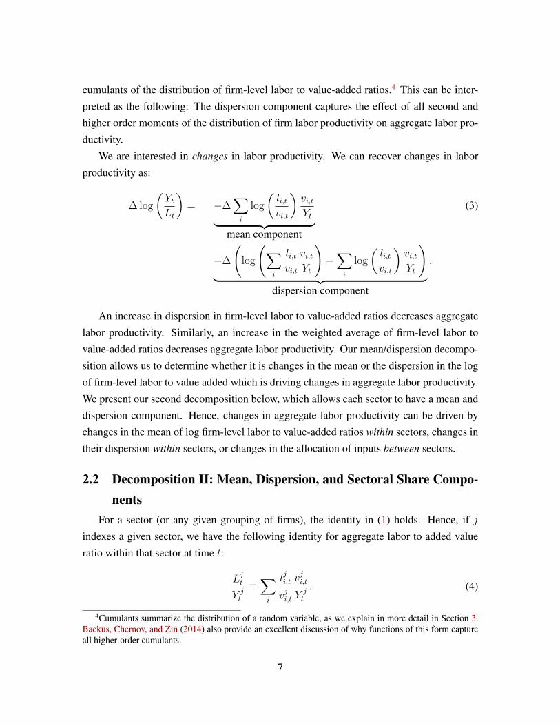
We are interested in changes in labor productivity. We can recover changes in labor
productivity as:
∆ log
(YtLt
)= −∆
∑i
log
(li,tvi,t
)vi,tYt︸ ︷︷ ︸
mean component
(3)
−∆
(log
(∑i
li,tvi,t
vi,tYt
)−∑i
log
(li,tvi,t
)vi,tYt
)︸ ︷︷ ︸
dispersion component
.
An increase in dispersion in firm-level labor to value-added ratios decreases aggregate
labor productivity. Similarly, an increase in the weighted average of firm-level labor to
value-added ratios decreases aggregate labor productivity. Our mean/dispersion decompo-
sition allows us to determine whether it is changes in the mean or the dispersion in the log
of firm-level labor to value added which is driving changes in aggregate labor productivity.
We present our second decomposition below, which allows each sector to have a mean and
dispersion component. Hence, changes in aggregate labor productivity can be driven by
changes in the mean of log firm-level labor to value-added ratios within sectors, changes in
their dispersion within sectors, or changes in the allocation of inputs between sectors.
2.2 Decomposition II: Mean, Dispersion, and Sectoral Share Compo-nents
For a sector (or any given grouping of firms), the identity in (1) holds. Hence, if j
indexes a given sector, we have the following identity for aggregate labor to added value
ratio within that sector at time t:
Ljt
Y jt
≡∑i
lji,t
vji,t
vji,t
Y jt
. (4)
4Cumulants summarize the distribution of a random variable, as we explain in more detail in Section 3.Backus, Chernov, and Zin (2014) also provide an excellent discussion of why functions of this form captureall higher-order cumulants.
7
In turn, for each sector at time t, we can decompose the aggregate labor to added value
ratio within a sector into a mean and dispersion component:
log
(Ljt
Y jt
)=∑i
log
(lji,t
vji,t
)vji,t
Y jt︸ ︷︷ ︸
Mjt
+
(log
(∑i
lji,t
vji,t
vji,t
Y jt
)−∑i
log
(lji,t
vji,t
)vji,t
Y jt
)︸ ︷︷ ︸
Djt
, (5)
where M jt is the static mean component in sector j and Dj
t is the static dispersion compo-
nent in sector j.
By an identity, aggregate labor productivity is equivalent to:
YtLt
=∑j
e−Mjt−D
jtLjtLt. (6)
This implies that aggregate labor productivity can be expressed as an aggregate of sec-
toral mean and dispersion components, weighted by the share of labor allocated to each
sector. Hence, when we look at changes in aggregate labor productivity, we have to ac-
count for the fact that input shares of different sectors can be changing over time. In turn,
we have a third component, which reflects changes in the input share of a given sector,
which we call the sectoral-share component:
log
(YtLtYt−1
Lt−1
)= log
∑
j
(e−M
jt
)Ljt−1
Lt−1∑j
(e−M
jt−1
)Ljt−1
Lt−1
︸ ︷︷ ︸
mean component
+ log
∑j e−Mj
t−DjtLjtLt∑
j e−Mj
t−DjtLjt−1
Lt−1
︸ ︷︷ ︸
sectoral share
+ log
∑j e−Mj
t−DjtLjt−1
Lt−1∑j e−Mj
t−1−Djt−1
Ljt−1
Lt−1
− log
∑
j
(e−M
jt
)Ljt−1
Lt−1∑j
(e−M
jt−1
)Ljt−1
Lt−1
︸ ︷︷ ︸
dispersion component
. (7)
In this decomposition, changes in aggregate labor productivity are broken into three
components. First, a mean component which captures changes in an aggregation of sectoral
mean log labor productivities. Second, a sectoral share component which captures the
effect of the changing allocation of labor between sectors. This second component will be
8
positive if labor is flowing from low labor productivity sectors to high labor productivities
onces. Third, a dispersion component, which captures changes in the dispersion of firm log
labor productivities within sectors.
2.3 Decomposing Changes in TFP using Decomposition IIWe measure TFP, At, as:
At =Yt
Kαt L
1−αt
. (8)
We assume that capital’s share of output, α, is positive. We can thus rewrite (8) as:
log(At) = α log(YtKt
) + (1− α) log(YtLt
). (9)
Taking changes in (9),
∆ log(At) = α∆ log(YtKt
) + (1− α)∆ log(YtLt
). (10)
In (7), we showed that changes in log( YtLt
) can be broken into mean, dispersion, and sectoral-
share components. Denote these components for labor as MLt , D
Lt , and SLt , respectively.
Denote these components for capital as MKt , D
Kt , and SKt , respectively. Hence,
∆ log(YtKt
) = MKt +DK
t + SKt . (11)
In turn, we can rewrite changes in log TFP from (10) as changes in the weighted sum
of the mean components for capital and labor, the dispersion components for capital and
labor, and the sectoral-share components for capital and labor:
∆ log(At) = (αMKt + (1− α)ML
t ) + (αDKt + (1− α)DL
t ) + (αSKt + (1− α)SLt ). (12)
3 Decomposition Applied to Models
In this section, we demonstrate the economics of our decomposition in standard produc-
tion environments. First, in the production environment described by Hsieh and Klenow
(2009), we demonstrate that changes in the production technology, prices, or the expected
value of the log of marginal revenue products of capital will manifest themselves in the
9
mean component of our decomposition. Second, changes in the variance or higher order
moments of the log of marginal revenue products of capital will be reflected in the disper-
sion component of our decomposition.
Building on the above results, we demonstrate in a standard production environment
how the components of our decomposition capture changes in the distribution of distor-
tions to firm labor and capital choices. We find that common changes to the frictions to
input choices facing firms are reflected in movements in the mean component. We also
derive conditions under which distributional changes in such frictions are reflected in the
dispersion component of our decomposition. Such results are derived in a more general
framework than that of Hsieh and Klenow (2009), and we identify a number of relevant
papers that can be mapped into our environment.
Our results are particularly relevant to the literature that studies the role financial fric-
tions play in amplifying movements in aggregates over the business cycle. We analytically
demonstrate how a change in a financial friction in a simple model of production will
present itself as a distortion. We then demonstrate that an increase in the extent to which
this financial friction affects firms will increase the dispersion in wedges.
3.1 Hsieh and Klenow (2009) Production EnvironmentThe model consists of heterogeneous firms that produce differentiated goods. There are
S industries, and the outputs of each industry, YS , are aggregated into a final good (total
output), Y , using Cobb-Douglas technology in a perfectly competitive market. Hence,
aggregate output can be defined as:
Y = ΠSs=1Y
θss , where
S∑s=1
θs = 1. (13)
From standard arguments: PSYS = θsPY , where the price of industry output is Ps and
P is the price of the final good, which is set to be the numeraire.
There areMs firms in a sector s. Industry output, Ys is produced using CES technology:
Ys =
(Ms∑i=1
Yσ−1σ
si
) σσ−1
. (14)
Within an industry, firms are heterogeneous in a few dimensions. First, they vary in
aspects of their physical productivity. Second, they vary in the magnitude of frictions to
10
their labor and capital choices. One can write these two distortions as distortions that
affect the marginal products of labor and capital evenly, which one can write as an output
distortion τY , and distortions that affect the marginal product of capital relative to labor,
which one can write as a capital distortion, τK . Firm i within sector s produces output, Ysi,
from its firm TFP, Asi, capital stock Ksi, and labor Lsi, using the following Cobb-Douglas
technology:
Ysi = AsiKαssi L
1−αssi . (15)
Profits of firm i in sector S are thus:
πsi = (1− τYsi)PsiYsi − wLsi − (1 + τKsi)RKsi. (16)
From standard arguments, in this setup, the marginal revenue product of capital for a
firm, MRPKsi ,∂PsiYsi∂Ksi
, is a function of the rental rate of capital and firm level wedges:
MRPKsi = R1 + τKsi1− τYsi
. (17)
As in Hsieh and Klenow (2009), it is useful to define the marginal product of capital (in
total) for a sector as the following:5
MRPKs ,R∑MS
i=1
1−τYsi1+τKsi
KsiKS
. (18)
For our decomposition, it is also useful to define the weighted average of the log
marginal product of capital for firms in a sector, which is:
LMRPKs ,MS∑i=1
log(R1 + τKsi1− τYsi
)PsiYsiPSYS
. (19)
5There was an error in the specification of this object in the original paper of Hsieh and Klenow (2009).The specification here corresponds to the form in the published corrections.
11
3.1.1 Our Decomposition in this Production Environment
In the environment above, from (18) and (19) and the definition of the marginal revenue
product of capital, our decomposition applied to capital productivity for sector s can be
expressed as the following:
∆ log
(P st Y
st
Kst
)= ∆ log
(1
αs
σ
1− σ
)+ ∆LMRPKs︸ ︷︷ ︸
mean component
+ ∆ log(MRPKs
)−∆LMRPKs︸ ︷︷ ︸
dispersion component
. (20)
We now demonstrate how the changing distribution of marginal productivities are re-
flected in our decomposition by demonstrating which cumulants of the distribution of log
marginal revenue productivities show up in which components of our decomposition. Cu-
mulants are similar to moments; the cumulant-generating function of a random variable
is an alternative specification of a probability distribution, similar to a moment-generating
function. The first cumulant is the expected value of the variable, the second cumulant is
its variance, and the higher order cumulants are polynomial combinations of centralized
moments. Consider the distribution of firm log marginal revenue products of capital, re-
flecting both the mass of firms at a given productivity and their relative output shares (to
be precise, the CDF would be written Gs (X) =∫i∈s 1 (MRPKsi ≤ X) PsiYsi
PSYSdi). Denote
the cumulants of this distribution as κs1, κs2, .... Using properties of the cumulant generating
function, our decomposition can be expressed as the following function of the cumulants
of the distribution of log marginal revenue productivities of capital:6
∆ log
(P st Y
st
Kst
)= ∆ log
(1
αs
σ
1− σ
)+ ∆κs1︸ ︷︷ ︸
mean component
+−∆κs22!
+∆κs33!− ∆κs4
4!+ ...︸ ︷︷ ︸
dispersion component
. (21)
Note that κs1 = LMRPKs is the weighted average of the log of firm marginal revenue
products of capital, while κs2 is the variance of the log of firm marginal revenue prod-
ucts of capital. The mean component captures only changes in technology or LMRPKs.
6See Appendix A for details of this derivation.
12
Changes in the second cumulant (and thus second central moment), or higher order cumu-
lants (and thus all of the remaining higher order moments) of the distribution of the log of
firm marginal revenue products of capital are reflected in the dispersion component of our
decomposition.
Note that if firm marginal revenue products of capital are lognormally distributed, then
only the first two cumulants are non-zero. In that case, our decomposition is isomorphic to a
mean-variance decomposition. Increases in the expected value of the log of firm marginal
revenue productivities are reflected in the mean component of our decomposition, while
the negative effect of the greater variance of the log of firm marginal revenue products is
reflected in the dispersion component of our decomposition. This is apparent if in (21) the
dispersion component is further broken into variance and higher order terms as below:
∆ log
(P st Y
st
Kst
)= ∆ log
(1
αs
σ
1− σ
)+ ∆κs1︸ ︷︷ ︸
mean component
+
variance︷ ︸︸ ︷−∆κs2
2!+
higher-order terms︷ ︸︸ ︷∞∑n=3
(−1)n−1 ∆κsnn!︸ ︷︷ ︸
dispersion component
. (22)
Notice, if we define κL,n as the n′th cumulant of the log of the marginal revenue product
of labor and κK,n as the n′th cumulant of the log of the marginal revenue product of capital,
we can apply our decomposition to changes in TFP using (12):
∆ log (TFPRs) = ∆ log
(σ
1− σα−αss (1− αs)αs−1
)+ (1− αs)∆κsL,1 + αs∆κ
sK,1︸ ︷︷ ︸
mean component
variance︷ ︸︸ ︷−
(1− αs)∆κsL,2 + αs∆κsK,2
2!+
higher-order terms︷ ︸︸ ︷∞∑n=3
(1− αs)∆κsL,n + αs∆κsK,n
(−1)n−1 n!︸ ︷︷ ︸dispersion component
.
(23)
13
3.2 Simple Model of Production and AllocationGiven an increase in the dispersion of wedges likely results in a change in value added
shares, we demonstrate under what conditions we can analytically demonstrate that an
increase in the dispersion of wedges leads to an increase in the dispersion component of
our decomposition. Similarly, we demonstrate under what conditions we can analytically
demonstrate that an increase in the mean of wedges will increase the mean component of
our decomposition, all else equal. We present our results within a similar environment to
Hsieh and Klenow (2009), but more general technology.
As in Hsieh and Klenow (2009), the model consists of heterogeneous firms who pro-
duce differentiated goods, which are aggregated into a final good (total output), but now
with a more general aggregation technology to be described below. Firms are heteroge-
neous in the following dimensions: They vary in aspects of their physical productivity, zit,
and they vary in the magnitude of frictions to their labor and capital choices.
3.2.1 Intermediate Good Firm Technology
Firms are indexed by i and time by t. Firm i at time t produces yi,t units of an intermedi-
ate good using li,t units of homogeneous labor and ki,t units of capital with the production
function yi,t = zi,tlγi,tk
νi,t. Labor and capital are homogeneous, therefore aggregate labor
and capital clearing imply that∫ili,tdi = Lt and
∫iki,tdi = Kt, where Lt and Kt denote
aggregate labor and capital.
3.2.2 Aggregation Technology and Value Added
Total output, Yt, is aggregated from firm output with technology Yt =(∫
iyϕi,tdi
)φ. Note
that this general form nests the two most common final good technologies considered in
the literature as special cases: The CES aggregator and heterogeneous firms producing a
single good. The final good sector is competitive and cost minimizing. Standard arguments
imply the price of each intermediate good, pi,t, is pi,t = Yφ−1φ Pt (yi,t)
ϕ−1, where Pt is the
price of the final good, which we set to be the numeraire. Therefore value added in real
terms, vi,t =pi,tPtyi,t, can be expressed as a function of prices and firm output:
vi,t = Yφ−1φ
t (yi,t)ϕ . (24)
To compute our decomposition, one requires firm-level productivity ratios and firm-
level value-added shares. For a given firm, we can compute a firm-level value-added share
14
as: vi,tYt
.
3.3 The Optimal Allocation of Inputs and the Role of Firm-level WedgesIn this subsection, we solve the optimal allocation of resources in the planner’s problem,
and we demonstrate how firm-specific wedges can distort the allocation of labor and capital
between firms from this allocation.
We show that the optimal allocation of resources in the planner’s problem is such that
all firms have the same productivity ratios. This choice is unique and can be characterized
as a function of the distribution of firm-level TFP, F zt (z). We then show that any allocation
of capital and labor between firms can be expressed as a function of the optimal input
choice and firm-specific wedges. We utilize this final result in the following subsection to
evaluate how shocks to firm-level wedges show up in our decomposition.
3.3.1 Optimal Allocation
We now present a proposition that highlights the known result that for any fixed amount
of total capital and labor, the optimal allocation of resources (to maximize static output)
is such that all firms with identical production function coefficients have the same factor
productivity ratios.
Proposition 1.
(i) Given a fixed amount of total labor and capital, Lt and Kt, the allocation of capital
and labor across firms that maximizes output is such that there are unique optimal
labor and capital productivity ratios, v∗t
l∗tand v∗t
k∗t, which are common among all firms
and only depend on the CDF of firm productivity, F zt (z).
Proof. See Appendix A.
A full (static) planner’s problem maximizing current welfare could be split into two
parts: First, solve for the optimal allocation rule of capital and labor between firms for any
fixed amount of both capital and labor; and second, choose the total amount of capital and
labor to maximize current period utility. Therefore Proposition 1 implies that the allocation
which maximizes static utility is one where firms have constant productivity ratios. We do
not place any restrictions on the level of statically optimal total labor and capital.
15
3.3.2 Firm-Level Wedges
We then use the optimal labor and capital productivity ratios to define firm-level wedges,
defined as the firm productivity ratio, vi,tli,t
or vi,tki,t
, over the optimal productivity ratio, v∗t
l∗tor
v∗tk∗t
. We formally define firm level wedges as:
ωl,i,t ,vi,tli,t
l∗tv∗t, (25)
and
ωk,i,t ,vi,tki,t
k∗tv∗t, (26)
for labor and capital, respectively.
These wedges capture how far a firm’s productivity ratio is from the one that maximizes
welfare in the social planner’s static optimization problem. They also capture aggregate
distortions, which distort every firm’s input decision and change aggregate labor or capital,
as well as changes in the relative distribution of resources between firms.
In the model of Hsieh and Klenow (2009), which is a special case of this production
environment, these wedges can be expressed as functions of the firm-level distortions in
their model, τY si and τKsi. The firm-level wedges are proportional to these distortions:
ωl,i,t ∝ 11−τY si
and ωk,i,t ∝ 1+τKsi1−τY si
.
3.4 Shocks to Firm-level Wedges in our DecompositionsIn this subsection, we illustrate how changes to the distribution of firm-level wedges
are captured in our decomposition and how such changes affect aggregates. The model
of production and allocation (from subsection 3.2) we consider only has a single sector of
production with identical production function coefficients, so we can perform our analysis
using Decomposition I. However, Decomposition II first applies Decomposition I individ-
ually to each sector and then aggregates up the sectoral mean and dispersion components.
Therefore, the way in which our components capture firm-level wedges will be similar for
a multi-sector version of our model with production function coefficients varying across
sectors. We perform our analysis of shocks to firm-level wedges only for Decomposition I
due to the greater tractability and cleaner demonstration of the economics of our decompo-
sition.
We begin without making parametric assumptions on the distribution of wedges. Let
16
Y ∗t
K∗t
denote the undistorted (absent any idiosyncratic or common distortions) aggregate cap-
ital factor productivity ratio. Let Fω,k denote the density function of wedges to firm cap-
ital choices, which reflects both the mass of firms and their relative value added shares.
Formally, this can be expressed as an integral over firms (denoted by i): Fω,k (x) =∫i1(ωk,i≤x)
viYdi. The cumulants of the log of firm-level wedges are denoted as: κk,1,t, κk,2,t,
κk,3,t, et cetera. Cumulants are similar to moments; we discuss their statistical properties in
subsubsection 3.1.1. Our decomposition of changes in aggregate capital productivity can
be expressed as:7
∆ log
(YtKt
)= ∆ log
(Y ∗tK∗t
)+ ∆κk,1,t︸ ︷︷ ︸
mean component
+
variance︷ ︸︸ ︷−∆κk,2,t
2!+
higher-order terms︷ ︸︸ ︷∞∑n=3
(−1)n−1 ∆κk,n,tn!︸ ︷︷ ︸
dispersion component
. (27)
Equation (27) shows that the mean component captures changes in the undistorted pro-
ductivity ratio (capturing changes unrelated to distortions) and changes in the first cumu-
lant (which capture common changes in distortions). Changes in the variance of firm log
wedges (the second cumulant), or any higher moments of their distribution, are reflected in
the dispersion component. Such results easily carry over for labor productivity by replacing
capital for labor in (27).
We can then use (12) to express total factor productivity as a function of undistorted
TFP, TFP ∗t , and the cumulants of wedges to capital and labor:8
∆ log (TFPt) = ∆ log (TFP ∗t ) + α∆κk,1,t + (1− α) ∆κl,1,t︸ ︷︷ ︸mean component
(28)
variance︷ ︸︸ ︷−α∆κk,2,t + (1− α) ∆κl,2,t
2!+
higher-order terms︷ ︸︸ ︷∞∑n=3
α∆κk,n,t + (1− α) ∆κl,n,t
(−1)n−1 n!︸ ︷︷ ︸dispersion component
.
7See Appendix A for details of this derivation.8For this exercise, we make the standard assumption that TFP is measured as TFPt = Yt
Kαt L
1−αt
, where αis constant over time.
17
Equation (28) shows that the mean component captures changes in undistorted TFP and
changes in the first cumulants of log wedges (corresponding to the mean of log wedges).
The dispersion component captures changes in the variance or higher order moments of log
wedges.
In the remainder of this subsection, we present special cases of the results in (27) and
(28). We show how common changes in wedges and changes in technology are reflected in
the mean component of our decomposition. Finally, we show that changes in the variance
and higher-order moments of log wedges are captured in the dispersion component our
decomposition.9
3.4.1 Common Shocks to Distortions
We first show that common changes to distortions are reflected only in the mean compo-
nent of our decomposition. First, consider a shock, ξt+1, that affects firms evenly such that
ωk,t+1 = ξl,t+1ωk,t. This is the sort of shock that would arise, for example, from a distortion
to the rental rate of capital faced by all firms. Below, we show the effect of this shock on
aggregate capital factor productivity and TFP is reflected only in the mean component:
∆log(YtKt
) = log(ξk,t)︸ ︷︷ ︸mean component
,
and
∆log(TFPt) = α log(ξk,t)︸ ︷︷ ︸mean component
.
Only the mean component will change if the economy is hit by no other shocks. Such
results extend to the decomposition of labor productivity when we replace labor for capital.
3.4.2 Shocks to the Variance and Higher-order Moments of Distortions
Note that the second cumulant is the variance of log wedges, while all of the higher
order cumulants can be expressed as polynomial combinations of the second and higher-
order central moments. Therefore (27) and (28) imply that changes in the variance and any
higher-order moments of log wedges are reflected in the dispersion component, without
having to make any parametric assumptions.9These results follow directly from our decomposition and properties of cumulant generating functions;
an outline of their derivation are found in Appendix A.
18
To provide further intuition, we now demonstrate how shocks to the distribution of
wedges are realized in our decomposition under some standard parametric assumptions.
For example, if wedges to capital are lognormally distributed with mean µω,k,t and variance
σ2ω,k,t, then changes in aggregate capital productivity can be decomposed as:
∆ log
(YtKt
)= ∆ log
(Y ∗tK∗t
)+ ∆µω,k,t︸ ︷︷ ︸
mean component
+ −∆σ2
ω,k,t
2︸ ︷︷ ︸dispersion component
.
With the lognormal assumption, only the first and second cumulant exist. A typical way of
adding variation in higher-order central moments (and thus higher-order cumulants) is to
create a mixture of lognormals. If wedges to capital are modeled as a mixture of lognor-
mals, with weights λk,n,t on lognormal distributions with means µk,n,t and variances σ2k,n,t,
then we can express our decomposition as follows:
∆ log
(YtKt
)= ∆ log
(Y ∗tK∗t
)+ ∆
∑n
λk,n,tµk,n,t︸ ︷︷ ︸mean component
−∆∑
n λk,n,tσ2k,n,t
2−∆ log
(∑n
λk,n,te(µk,n,t−
∑j λk,j,tµk,j,t)e
12(σ2
k,n,t−∑j λk,j,tσ
2k,j,t)
)︸ ︷︷ ︸
dispersion component
.
The mean component captures changes in the weighted means of the lognormal distribu-
tions or in the undistorted factor productivity ratio. All other changes in the distributions
will be reflected in the dispersion component. Changes in the variances of the lognor-
mal distributions which make up the mixture will be reflected here, as will higher order
moments. For example, a skewed distribution is often parameterized as a mixture of log-
normals with different means, which will be reflected, via the term e(µk,n,t−∑j λk,j,tµk,j,t), in
the dispersion component. Kurtosis is often often parameterized as a mixture of lognormals
with different variances, which will be reflected, via the term e12(σ2
k,n,t−∑j λk,j,tσ
2k,j,t), in the
dispersion component.
3.5 Mapping to Other ModelsIn this subsection, we show that our model has a mapping to several models of frictions
to the allocation of labor and capital between firms. We then demonstrate how frictions in
19
a simple model of financial frictions would be reflected in wedges, and then discuss how
our decomposition would capture changes in such frictions.
3.5.1 Mapping to Models of Labor or Capital Allocation
Our simple model consists only of a production environment with wedges representing
frictions to the allocation of labor and capital. Therefore, there is a mapping to any model
with a production environment consistent with ours. This includes the models of Khan and
Thomas (2013), Bloom et al. (2014), and Arellano et al. (2012), as well as numerous other
heterogeneous agent models considered in the macroeconomics literature.
We formally show this correspondence by proving that given the production environ-
ment in our model, aggregate output, employment, capital, and the full distribution of out-
put, labor, capital, and technology across firms can be characterized using wedges and
either firm-level technology or output shares for any allocation of labor, capital, and tech-
nological productivity across firms. We denote Gt (z, ωl, ωk) as the joint distribution of
firm technological productivity and firm-level wedges to labor and capital, Jt(vY, ωl, ωk
)as the joint distribution of firm output shares and firm-level wedges to labor and capital,
and Zt =
(∫i
(zϕ( 1
1−νϕ−γϕ)i,t
)di
)φ(1−νϕ−γϕ)
as an index of aggregate productivity. The
following proposition states that this representation can map any resulting allocation of
resources and aggregates using these firm-level wedges:
Proposition 2. The full distribution of labor, capital, and productivity across firms, Ft (z, l, k),
and aggregate output, employment, and capital have a 1-1 mapping with any of the follow-
ing:
(i) Gt (z, ωl, ωk).
(ii) Jt(vY, ωl, ωk
)and a measure of aggregate productivity Zt.10
Proof. See Appendix A.
3.5.2 Mapping to a Model of Financial Frictions
In this subsection, we show that a financial friction in a simple model map can be
redefined as a firm-level wedge. We then discuss how a tightening of the friction in the
model can generate a greater variance of wedges.
10More generally, it can be shown that Jt(vY , ωl, ωk
)together with
(∫zτdF z(z)
), for any τ 6= 0, is
sufficient to characterize output, employment, and capital at both the aggregate and firm level.
20
Consider a simple model where heterogeneous firms produce a homogeneous consump-
tion good with technology yi,t = zi,tlbi,t, where b < 1. In this setting, value added is equiva-
lent to firm output, vi,t = zi,tlbi,t. Households have utility function U (C,L) = C1−σ
1−σ −L1+ν
1+ν
and discount the future at rate β. Production in this simple model is a special case of the
production environment introduced in Subsection 3.2; thus, the planner’s problem states all
firms optimally have the same labor productivity ratios.
The friction in this model is a simple borrowing constraint: Firms have wealth ai,t,
which we consider exogenous for our analysis. Firms must pay their workers at the begin-
ning of the period but only receive cash flows from production at the end. The borrowing
constraint, li,tW ≤ ai,tρ, where W is the wage and ρ is a positive constant, restricts the la-
bor decisions of firms when it binds. Assume firms may also exogenously exit each period
with probability δ.
The optimization problem of firms can be expressed as the following Lagrangian:
L = maxli,t
zi,tlbi,t − li,tW + λi,t (ai,tρ− li,tWt) , (29)
where λi,t is the Lagrange multiplier on the borrowing constraint. The multiplier is 0
if the borrowing constraint does not bind, and positive otherwise. Taking the first-order
conditions of (29) and manipulating the labor-leisure condition allows us to express the
firm’s labor choice as the following:
li,t = z1
1−bi,t b
11−bY
− σ1−b
t L− ν
1−bt (1 + λi,t)
− 11−b . (30)
From (30) we can derive firm-level wedges, ωl,i,t =vi,tli,t
l∗tv∗t
, as a function of aggregates
and the Lagrange multiplier faced by the firm:
log (ωl,i,t) = σlog
(YtY ∗t
)+ νlog
(LtL
∗t
)︸ ︷︷ ︸
Aggregate
+ log (1 + λi,t)︸ ︷︷ ︸FirmSpecific
. (31)
Note that the wedge can be expressed as a function of the distortion of aggregates
from their optimal value (which affect the wage rate) as well as the firm-specific distortion
captured by the Lagrange multiplier in the firm’s problem. We can express the Lagrange
multiplier as the following function of aggregates and each firm’s zi,t and ai,t:
21
log (1 + λi,t) =
0 zi,tbY−bσt L−bνt ab−1
i,t ρb−1 ≤ 1
log(bY −bσt L−bνt zi,ta
b−1i,t ρ
b−1)
zi,tbY−bσt L−bνt ab−1
i,t ρb−1 > 1
. (32)
Note that the only way that there is no heterogeneity in Lagrangian multipliers is either
if (a) the borrowing constraint never binds, or (b) it binds for all firms, but wealth is propor-
tional to productivity (zi,t = a1−bi,t ). This second condition implies no inefficiencies in the
distribution of resources between firms; all inefficiencies arise from the reduced aggregate
demand for labor.
Now consider what a shock to borrowing constraints does. Assume that at time t = 0,
ρ is high enough such that the constraint binds for no firms. Then the mean and variance of
log (1 + λi,0) is 0. A decrease in ρ to the point where the constraint binds for some but not
all firms leads to a rise in both the mean and variance of log (1 + λi,t). At the same time, the
borrowing constraint reduces Yt and Lt, as some firms cannot hire the amount of labor they
would prefer were they unconstrained. Therefore the change to the mean of firm wedges,
log (ωl,i,t), as a result of this shock is ambiguous, as the aggregate component and the mean
of the firm-specific component move in opposite directions. However, the direction of the
change in variance of the firm-level labor wedge is unambiguous, increasing in response to
such a shock.
4 Decomposition Applied to DataIn this section, we apply our decompositions of aggregate productivity described in
Section 2 to data on U.S. public firms and Japanese public firms. In our discussion of the
results applied to U.S. public firms, we also include a comparison of our measures of labor
productivity, capital productivity, and TFP to those from the national income and product
accounts (NIPA). In Appendix B, we describe how we clean our data on U.S. nonfinancial
public firms, and measure the objects of interest.
4.1 Discussion of results — Data from the United StatesFigures 1 and 2 display results of year-over-year changes in aggregate labor productivity
and its components from Decompositions I and II, respectively. From the eye test alone it
should be clear that in the recent recession, aggregate labor productivity and its dispersion
component have a negative correlation, and the mean component is highly correlated with
22
aggregate labor productivity. Figures 3 and 4 further demonstrate this point: Over four
recession periods, the mean component moves closely with aggregate labor productivity.
In Decomposition II, the dispersion component has very little cumulative change over any
of the four episodes in our sample.
Figures 5 and 6 display results from Decompositions I and II of year-over-year changes
in aggregate capital productivity, and tell a different story. The dispersion component is
positively correlated with aggregate capital productivity over the past two business-cycle
episodes. For previous episodes, the mean component moves more closely with aggregate
capital productivity. These results are more starkly apparent in Figures 7 and 8, which show
cumulative changes in aggregate capital productivity and its components from Decompo-
sitions I and II. In the recent episodes, for either decomposition, the dispersion component
moves much more closely with aggregate capital productivity.
As we describe in the previous subsection on measurement, to compute TFP, by the
nature of our assumptions on the production function and values for its coefficients, changes
in labor productivity get more weight (65 percent) than changes in capital productivity (35
percent). Hence, as should be expected, we see that the results for TFP are much more
qualitatively consistent with the results from what drives changes in labor productivity.
This is apparent in the year-over-year changes charts from Decompositions I and II in
Figures 9 and 10, as well as the cumulative changes charts from Decompositions I and II
in Figures 11 and 12.
Table 1 displays correlations between the components of Decomposition II and their
respective aggregates. The results from the figures are further codified in this table. The
correlation between the dispersion component and sectoral share components and labor
productivity are especially striking. Movements in labor productivity are much more cor-
related with the mean of firm-level log labor to value-added ratios than with their disper-
sion. These results are dampened when looking at TFP because capital productivity has a
positive correlation with its dispersion component. However, the relationship between TFP
and its dispersion component is ultimately close to zero.
Our sample represents a significant slice of the U.S. economy; in 2011, it accounted
for over 15 percent of GDP and over 17 million employees. To understand the extent to
which our sample reflects the mechanisms responsible for driving aggregate productivity
changes, we compare the time-series behavior of each aggregate productivity ratio as ag-
gregated from Compustat to that of the respective productivity ratio computed from NIPA.
Figures 16 and 17 show that the time-series properties of TFP computed from both Com-
23
pustat and NIPA are similar both in their cyclical dynamics and long-term trends. These
figures suggest that some of the key forces driving TFP over time are likely present in Com-
pustat data. If there were significant factors driving TFP over the business cycle that existed
only in small, private firms, we would expect systematic differences in the behavior of TFP
and our measure computed from publicly listed firms over time. However, there are some
differences in the measures. TFP from Compustat is more volatile, which is unsurprising
given the documented greater volatility of corporate profits measured with generally ac-
cepted accounting principles (GAAP) than corporate profits as measured in NIPA.11 There
are also some slight timing differences, particularly in the timing of the trough (of TFP) of
the 2007—2009 recession. These timing differences may be due to the reporting dates of
firms in Compustat. However, the measure of TFP for the United States in the Penn World
Tables (8.0) has the trough in 2009, so the timing differences may also be due to some tech-
nical adjustments made in the NIPA aggregation. In Figures 18 and 19, we look at changes
in each productivity ratio and its NIPA equivalent. We see the timing and volatility issues
are present for each productivity ratio separately.
4.2 Discussion of results - Data from JapanIn Figures 13 and 14, we display results from Decompositions I and II of year-over-year
changes in aggregate TFP in Japan. The results from the second decomposition are more
consistent with those from the United States for the recent recession in that the dispersion
component is not correlated with movements in TFP. The results from the first decomposi-
tion, however, show the dispersion component to be more highly correlated with aggregate
TFP over the recent episode. This result is true for labor productivity as well.
5 ConclusionThis paper presents decompositions of changes in aggregate labor productivity, capital
productivity, and TFP. We demonstrate how the dispersion component of our decomposi-
tions reflects changes in the degree to which frictions affect firms in many heterogeneous
firm models that attempt to explain the nature of the business cycle. In turn, computing
the components of our decomposition in data and comparing them to the same metrics in a
given model of the class we consider will help to assess whether such a model is consistent11Hodge (2011) compares the properties of corporate profits computed from the GAAP accounting state-
ments of firms in the S&P 500 index with the corresponding measure from NIPA, finding significantly greatervolatility in the S&P measure.
24
with firm-level behavior. As we demonstrate in this paper, it is not only useful to com-
pute our decompositions on models that have already been solved; one can also compute
our metrics in the data before writing down a model to help motivate which mechanisms
should be key in driving patterns over the business cycle.
Appendix A
Proof for Proposition 1Given the model of production in Subsection 3.2, we can define the following La-
grangian for the social planner to solve supposing she gets to allocate a fixed amount of
labor and capital across firms, which are indexed by i:12
L = maxli,ki
(∫i
(zilγi k
νi )ϕ di
)φ+ λ1
(K −
∫kidi
)+ λ2
(L−
∫lidi
). (33)
We want to show that there exists optimal labor and capital productivity ratios that are
shared by all firms that share the same production function coefficients. From the first-order
conditions of (33):
νϕφY1−φφ
(zilγi k
νi )ϕ
k= λ1, (34)
and
γϕφY1−φφ
(zilγi k
νi )ϕ
l= λ2. (35)
Also, the planner will fully allocate labor and capital to all firms, so:
K =
∫kidi, (36)
and
L =
∫lidi. (37)
12To economize on notation, time subscripts are omitted.
25
With some algebra, it can be shown that:
vi = kiλ1
νϕφ, (38)
and
vi = liλ2
γϕφ. (39)
Hence, summing over i in (38) and (39):
Y = Kλ1
νϕφ, (40)
and
Y = Lλ2
γϕφ. (41)
In turn, from (38) and (40):
Y
K=viki. (42)
Also, from (39) and (41):
Y
L=vili. (43)
In turn, all firms will optimally have the same firm-level capital and labor productivity
ratios.
We can now express optimal productivity ratios v∗
l∗and v∗
k∗as a function of L, K, and
Y ∗.
From the production technology, (42), and (43):
ki = Y−1φ zϕi l
ϕγkϕνi K∗ (F z(z)) , (44)
and
li = Y−1φ zϕi l
ϕγkϕνi K∗ (F z(z)) . (45)
26
Combining the production technology with (44) and (45), along with some algebra, yields:
Y ∗ = LϕφγKφϕν
(∫i
(zϕ( 1
1−νϕ−γϕ)i
)di
)φ(1−νϕ−γϕ)
. (46)
Note that this optimal output is just a function of the distribution of productivity, F z(z),
and total labor and capital.
Thus, we can express the optimal productivity ratios as:
v∗
l∗=Y ∗
L, (47)
and
v∗
k∗=Y ∗
K. (48)
Proof for Proposition 2This proof is done in the following parts:
(i) F (z, l, k) fully characterizes output, employment, and capital.
(ii) F (z, l, k) has a 1-1 mapping with G(z, ωl, ωk).
(iii) G(z, ωl, ωk) has a 1-1 mapping with J( vY, ωl, ωk) and a measure of aggregate pro-
ductivity Z =
(∫i
(zϕ( 1
1−νϕ−γϕ)i
)di
)φ(1−νϕ−γϕ)
.
Part (i): F (z, l, k) fully characterizes output, employment, and capital.
This must be true, by the definition of production technology and the clearing con-
ditions L =∫ldF (z, l, k) and K =
∫kdF (z, l, k). Thus, F (z, l, k) fully characterize
aggregate output, employment, and capital.
Part (ii): F (z, l, k) has a 1-1 mapping with G(z, ωl, ωk).
The portion of the proof has the following parts:
(a) F (z, l, k) has a unique mapping χ1 into G(z, ωl, ωk).
(b) G(z, ωl, ωk) has a unique mapping χ2 into F (z, l, k).
(c) χ2 = χ−11 .
27
F (z, l, k) has a unique mapping χ1 into G(z, ωl, ωk):(24) combined with the production technology gives us vi as a function of only z, l, k:
vi =
(∫zϕlγϕkνϕdF (z, l, k)
)φ−1
zϕi lγϕi kνϕi . (49)
Combining (25), (26), and (49) yields:
ωk (zi, li, ki, F ) =
(∫zϕlγϕkνϕdF (z, l, k)
)φ−1zϕi l
γϕi kνϕi
ki
k∗
v∗, (50)
and
ωl (zi, li, ki, F ) =
(∫zϕlγϕkνϕdF (z, l, k)
)φ−1zϕi l
γϕi kνϕi
li
l∗
v∗. (51)
These equations characterize the wedges implied by a given distribution of capital,
labor, and productivity. We can rearrange (50) and (51) to solve for labor and capital as a
function of wedges:
k (zi, ωl,i, ωk,i, F ) =
((∫zϕlγϕkνϕdF (z, l, k)
)φ−1zϕi(l∗
v∗
)γϕ (k∗v∗
)1−γϕ
(ωl.i)γϕ (ωk,i)
1−γϕ
) 11−γϕ−νϕ
, (52)
and
l (zi, ωl,i, ωk,i, F ) =
((∫zϕlγϕkνϕdF (z, l, k)
)φ−1zϕi(l∗
v∗
)1−νϕ (k∗v∗
)νϕ(ωl,i)
1−νϕ (ωk,i)νϕ
) 11−γϕ−νϕ
. (53)
(52) and (53) allow us to obtain the unique mapping from F to G:
G (z, ωl, ωk) =
∫ z,ωl,ωk
z,ωl,ωk=0
dF (z, l (z, ωl, ωk, F ) , k (z, ωl, ωk, F )) . (54)
G(z, ωl, ωk) has a unique mapping χ2 into F (z, l, k):
28
Combining (50) and (51) allows us to express F (z, l, k) as the following:
F(z, l, k
)=
∫ z,l,k
z,l,k=0
dG (z, ωl (z, l, k, F ) , ωk (z, l, k, F )) . (55)
This expression is not sufficient to characterize F (z, l, k) as a function of G(z, ωl, ωk),
as the functions ωl() and ωk() on the right-hand side depend on the term(∫zϕlγϕkνϕdF (z, l, k)
)φ−1φ . Note that
(∫zϕlγϕkνϕdF (z, l, k)
)φ−1φ = Y
φ−1φ . All we have
to do now is express Y as a function of G. Plugging (52) and (53) into the aggregate
production function yields:
Y =
(k∗v∗
)ϕφν (l∗
v∗
)ϕφγ (∫z
ϕ1−γϕ−νϕ
ωγϕ
1−γϕ−νϕl ω
νϕ1−γϕ−νϕk
dG (z, ωl, ωk)
)φ
1−γϕ−νϕ1−φ(γϕ+νϕ)
.
(56)
Y (G (z, ωl, ωk)) can thus be defined as a function of z and wedges.
(55) and (56) can be combined to obtain the functions ωl (z, l, k, G) and ωk (z, l, k, G).
Thus, we can obtain the unique mapping:
F(z, l, k
)=
∫ z,l,k
z,l,k=0
dG (z, ωl (z, l, k, G) , ωk (z, l, k, G)) . (57)
χ2 = χ−11 :
Combining (54) and (57) yields the result that F (z, l, k) = χ2 (χ1 (F (z, l, k))) for any
F (z, l, k). It follows that χ2 = χ−11 .
Part (iii): Claim: G(z, ωl, ωk) has a 1-1 mapping with J( vY, ωl, ωk) and a measure of
aggregate productivity Z =
(∫i
(zϕ( 1
1−νϕ−γϕ)i
)di
)φ(1−νϕ−γϕ)
.
The portion of the proof has the following parts:
(a) G(z, ωl, ωk) has a unique mapping χ3 into J( vY, ωl, ωk) and pins down Z.
(b) J( vY, ωl, ωk) and Z has a unique mapping χ4 into G(z, ωl, ωk).
(c) χ3 = χ−14 .
29
G(z, ωl, ωk) has a unique mapping χ3 into J( vY, ωl, ωk) and pins down Z:
(49), (52), (53), and (56) can be combined to characterize vY
:
viY
=z
ϕ1−γϕ−νϕi (ωl,i)
−γϕ1−γϕ−νϕ (ωk,i)
−νϕ1−γϕ−νϕ∫
zϕ
1−γϕ−νϕ (ωl)−γϕ
1−γϕ−νϕ (ωk)−νϕ
1−γϕ−νϕ dG(z, ωl, ωk), (58)
and thus express z as a function of vY
, ωl, ωk, and G:
z(viY, ωl,i, ωk,i, G
)= ωγl,iω
νk,i
(viY
∫z
ϕ1−γϕ−νϕ
ωγϕ
1−γϕ−νϕl ω
νϕ1−γϕ−νϕk
dG (z, ωl, ωk)
) 1−γϕ−νϕϕ
.
(59)
(59) can be used to characterize J( vY, ωl, ωk):
J( vY, ωl, ωk
)=
∫ vY,ωl,ωk
vY,ωl,ωk=0
dG(z( vY, ωl, ωk, G
), ωl, ωk
). (60)
G (z, ωl, ωk) trivially maps into a unique Z.
J( vY, ωl, ωk) and Z has a unique mapping χ4 into G(z, ωl, ωk):
(59), rearranged and integrated, yields:
∫z
ϕ1−γϕ−νϕ
ωγϕ
1−γϕ−νϕl ω
νϕ1−γϕ−νϕk
dG (z, ωl, ωk) =Z
1φ(1−νϕ−γϕ)∫ (
vY
)ω
γϕ1−νϕ−γϕl ω
νϕ1−νϕ−γϕk dJ
(vY, ωl, ωk
) .. (61)
Combining (59) and (61) yields:
z(viY, ωl,i, ωk,i, J, Z
)= ωγl,iω
νk,i
viYZ
1φ(1−νϕ−γϕ)∫ (
vY
)ω
γϕ1−νϕ−γϕl ω
νϕ1−νϕ−γϕk dJ
(vY, ωl, ωk
)
1−γϕ−νϕϕ
. (62)
(62) implies that we can express G(z, ωl, ωk) as a function of J( vY, ωl, ωk) and Z:
G (z, ωl, ωk) =
∫ z,ωl,ωk
z,ωl,ωk=0
dJ( vY
(z, ωl, ωk, J, Z) , ωl, ωk
). (63)
30
χ3 = χ−14 :
These two mappings are trivially inverses of each other.
Other Derivations
Decomposition as a Function of Cumulants
Consider the cumulative density function of firm log capital productivity, weighted
by output shares, G (X) =∫i1
(log(viki
)≤ X
)viY
. The mean component expressed
as a function of this distribution is: −∫x−xdG (x), while the dispersion component is:
−(∫
e−xdG (x)−∫−xdG (x)
).
We know, by definition, that the first cumulant can be written as:∫xxdG (x). A prop-
erty of the cumulant generating function is that E [etx] =∑n
t=1 tn κnn!
, which yields:
∫e−xdG (x) =
n∑t=1
(−1)nκnn!
= −κ1 +n∑t=2
(−1)nκnn!.
Therefore the mean component can be written as:
−∫x
−xdG (x) = κ1.
While the dispersion component is:
−(∫
e−xdG (x)−∫−xdG (x)
)= −
(−κ1 +
n∑t=2
(−1)nκnn!
+ κ1
)
= −n∑t=2
(−1)nκnn!
=n∑t=2
(−1)n+1 κnn!.
This means our decomposition can be expressed as:
log
(Y
K
)= κ1︸︷︷︸
Mean Component
+−κ2 +n∑t=3
(−1)n+1 κnn!︸ ︷︷ ︸
Dispersion Component
.
Now note that for any variable of the form zi = c viki
(such as capital wedges or marginal
products in a Hsieh and Klenow case) yields log (zi) = log (c) + log(viki
). Standard
properties of cumulants imply that κ1,z = κ1, vk
+ log (c), and κn,z = κn, vk
for all n > 1.
31
Therefore for such variables, our decomposition implies
log
(Y
K
)= κ1,z − c︸ ︷︷ ︸
Mean Component
+−κ2,z +n∑t=3
(−1)n+1 κn,zn!︸ ︷︷ ︸
Dispersion Component
.
(21) and (27) follow immediately from this derivation.
Our Decomposition for Different Models and Shocks
Common changes in firm revenue products, whether driven by technology or distor-
tions, are reflected only in the mean component of our decomposition. Consider a change
in revenue products such that vi,t+1
ki,t+1= x
vi,tki,t
. Then, our decomposition implies that:
log
(Yt+1
Kt+1
)= −
∫log
(ki,tvi,t
1
x
)vi,tYtdi︸ ︷︷ ︸
mean component
−(log
(∫ki,tvi,t
1
x
vtYi,t
di
)−∫log
(ki,tvi,t
1
x
)vtYtdi
)︸ ︷︷ ︸
dispersion component
= log(x)−∫log
(ki,tvi,t
)vi,tYtdi︸ ︷︷ ︸
mean component
−(log
(∫ki,tvi,t
vtYi,t
di
)−∫log
(ki,tvi,t
)vtYtdi
)︸ ︷︷ ︸
dispersion component
.
The results in subsubsections 3.4.1 immediately follow from the above. The results in
subsubsection 3.4.2 can be derived by using standard formulas for the expectation of log-
normally distributed variables.
Specifically, consider the case where the output-share weighted distribution of wedges
is a mixture of lognormals. The pdf of wedges is thus g (log (ω)) =∑N
n=1 λnφn (log (ω)),
where φn, where φn are normal pdfs and∑
n λn = 1. Note that lognormal wedges is
the special case of this with N = 1. Standard formulas for expectations over lognor-
mal distributions imply that∫log (ω) g (log (ω)) dω =
∑n λnµn and
∫ωtg (log (ω)) dω =∑
n λnetµn+ 1
2t2σ2
n . The results in subsubsection 3.4.2 immediately follow.
Appendix B
Measurement of Objects — Data from the United StatesFor the empirical analysis in Section 4 on U.S. firms, we use annual data on firms that
exist in the Compustat database. We take the following steps, in order. First, firms must
32
be headquartered in the United States and have a U.S. currency code. We then keep only
firms with December fiscal year-ends. We then drop firms if their employment, property,
plant, and equipment — net of depreciation, sales, or our measure of firm-value added —
are missing or negative. We then exclude firms with 4-digit SIC codes between 4000 and
4999, between 6000 and 6999, or greater than 9000, as our model is not representative of
regulated, financial, or public service firms. We then clean the data by winsorizing each
series at the 1st percentile over the entire sample. For our analysis, we lastly only keep data
from 1971 to 2011.
Firm-level value added, firm-level capital stock, and firm-level employment are the
only firm-level objects we need for our decomposition. When computing year-over-year
changes in the components of our decomposition, we also adjust for entry and exit by only
keeping data on firms that exist in consecutive years. In the second decomposition, firms
are grouped into sectors by two-digit SIC codes.
We measure labor as the number of employees reported in Compustat. We measure
capital as the firm’s plant, property, and equipment, adjusted for accumulated depreciation.
The aggregate capital stock is annual, taken from the Penn World Tables. To adjust for
potential changes in the valuation of capital over time, we construct a perpetual inventory
measure of the aggregate capital stock and use the ratio of this measure to the value of the
aggregate capital stock to deflate the firm-level measure of capital. The investment measure
used in the perpetual inventory method is annual gross private domestic investment from
the Bureau of Economic Analysis (BEA). To construct our measure of capital using the
perpetual inventory method (starting from 1959), we use a depreciation rate of 4.64 percent
and growth rate of technology of 1.6 percent, following Chari, Kehoe, and McGrattan
(2007). Our measure is then deflated by the December value of the monthly CPI, which is
CPI for All Urban Consumers, seasonally adjusted, from the Bureau of Labor Statistics.
We create a measure of value added in public firms using income accounting. GDP has
an income equivalent, GDI, which has similar time-series properties. The major compo-
nents of this measure have equivalents to income statement measures that are required on
10-K forms for U.S. public firms. In order of magnitude, GDI is made up of the follow-
ing components: compensation of employees, net operating surplus, consumption of fixed
capital (depreciation), and taxes on production and imports less subsidies. While we do not
observe the taxes or subsidies on production and imports firms pay in our dataset, we do
observe measures of the other three components, all of which make up over 90 percent of
GDI for all years in our sample. We observe labor compensation in Compustat annually.
33
If labor compensation is missing, we replace it with selling, general, and administrative
expenses. We also observe net operating profits before depreciation, which is the sum of
a firm’s net operating surplus and its capital consumption. We define a firm’s contribution
to output as the sum of labor compensation and operating profits before depreciation. In
practice, the BEA uses a similar, more detailed approach, where they use firm tax data to
aggregate up the components of domestic income and make adjustments for differences
between accounting and economic treatment of factors such as capital consumption and
inventory valuation.
To compute TFP, following Chari, Kehoe, and McGrattan (2007), we set capital’s share
of income, α = .35 and back it out from (9). When we compare our measure against
the NIPA-equivalent, we require a NIPA equivalent measure of our value-added measure,
a measure of aggregate labor, and a measure of aggregate capital. To compute our NIPA
equivalent of our pseudo-GDI measure, we use data from NIPA table 1.12 on National
Income by Type of Account. We take compensation of employees (line 2) and subtract
government (line 4), then add to this measure corporate profits with inventory valuation
adjustment and capital consumption adjustment less taxes on corporate income (line 43).
Finally, we add to this measure consumption of fixed capital, which comes from the BEA.
All measures are quarterly, and we only use the fourth-quarter values of these measures.
We put this measure in per-capita terms using population including armed forces overseas.
This measure is mid-period and monthly. We only keep its December value. We then put
this measure in real terms using the CPI measure described in this subsection. Our measure
of the real aggregate capital stock was already described in this subsection. This measure is
also put in per-capita terms. Our measure of aggregate labor is total non-farm employment
and is monthly. We only use the December observation of this variable.
Measurement — Data from JapanOur data on Japanese public firms comes from the Compustat global database, and our
firm-level variables are measured annually. We clean the data as we do for data from the
United States, except we only keep firms with currency codes corresponding to the Japanese
Yen and country headquarter codes corresponding to Japan. Also, the years of our sample
are different: They only cover 2001 to 2011. Consistent with our application to U.S. data,
when computing year-over-year changes in the components of our decomposition, we also
adjust for entry and exit by only keeping data on firms that exist in consecutive years. In
Decomposition II, firms are grouped into sectors by two digit SIC codes
34
As for the U.S. data, we measure firm-level labor as the number of employees reported
and firm-level capital as the firm’s plant, property, and equipment, adjusted for accumulated
depreciation. We deflate the firm-level Japanese capital stock by the U.S. capital deflater.
To put the capital stock in real terms, we deflate it by the OECD’s measure of the quarterly
CPI in Japan. We only keep the fourth-quarter value of this measure.
In a manner consistent with our application to U.S. data, we create a measure of value
added in public firms using income accounting, which is the sum of labor compensation
and operating profits before depreciation. As for the U.S. data, if labor compensation is
missing, we replace it with selling, general, and administrative expenses. We eventually
deflate by the same Japanese CPI measure as for capital. To compute TFP, we again set
α = .35 and back it out from (9).
Appendix C
Our Decomposition in the Context of Other Methodologies
To apply our decomposition to data, one does not need to estimate firm-level TFP or
sectoral production function coefficients. There is already potential for measurement is-
sues biasing the results from our decompositions, as measures of labor, value added, and
capital can all be measured incorrectly. Further, we could be incorrectly grouping firms
with our sectoral definitions. However, it is easy enough to check different measures of
labor, capital, or value added, if available, and see if the results change. Also, one could
add measurement error to firm variables and test the extent to which the results change.
Similarly, one can check the results from our second decomposition on different definitions
of “groupings” or sectors. However, to compute sectoral production function coefficients,
as is commonly done in papers assessing the role of labor and capital allocation on pro-
ductivity over the business cycle, some issues cannot be “checked.” Data from 30 years
prior can be crucial in providing “correct” estimates of sectoral production function coef-
ficients. But what if such data are unavailable to the researcher? In addressing the role of
resource reallocation in productivity dynamics over the business cycle, the literature has
relied on the estimation of these technological measures for all sectors in the economy. In
this section, we will demonstrate how some of the econometric biases associated with such
an approach can lead one to produce quantitatively and qualitatively different results on the
role of allocative efficiency over the business cycle.
35
We first demonstrate the most difficult-to-correct econometric bias associated with mea-
suring production function coefficients, which is the fact that data for the entire sector over
the entire sample are needed to estimate them. We also show that different definitions of
factor prices can crucially affect one’s results. Second, we show that our decomposition can
help to assess the role of resource reallocation in productivity dynamics over the business
cycle. In particular, in a relatively general setting, we demonstrate that the within-industry
component of our decomposition is reflective of within-sector allocative efficiency. Ulti-
mately, this section is meant to demonstrate that our decomposition can, at the very least, be
a useful check on such attempts at measuring the role of resource allocation over the busi-
ness cycle that require estimates of sectoral production function coefficients and firm-level
TFP.
Illustrating issues with identificationIn Figure 15, we demonstrate one possible issue with identification that can severely
change the interpretation of the qualitative and quantitative importance of the role of real-
location over the business cycle. We show that our results change substantially when we
follow a standard procedure and only slightly vary the estimation procedure for production
function coefficients.13 Figure 15 shows the cumulative change in the contribution of al-
locative efficiency to TFP over the recent recession for three different standard “versions”
of estimating production function coefficients.14 We estimate production function coeffi-
cients as the average of the ratio of capital expenditures to labor expenditures, rkwl
, across
firms within a sector over time, where r is the rental rate, k is the capital stock in the firm,
w is the wage, and l is labor utilization in the sector. In Version 1, the baseline version, we
drop all observations before 1972, use capital and labor utilization from our firm-level data,
and estimate the rental rate and wage following Chari, Kehoe, and McGrattan (2007).15
We see that in Version 1 of our estimation of production function coefficients, there
seems to be a decrease in allocative efficiency from pre-recession levels to the trough in13Specifically, we implement the approach of Oberfeld (2013) to measure changes in allocative efficiency
in our sample of U.S. publicly listed firms. This model of production and aggregation is identical to that inHsieh and Klenow (2009). Details of our dataset construction and measurement can be found in section 4and Appendix B. As in Oberfeld (2013) and Hsieh and Klenow (2009), we set the elasticity of substitutionwithin sectors to 3.
14Positive changes indicate an increase in the extent of allocative efficiency.15Following Chari, Kehoe, and McGrattan (2007) entails setting r = α∗ YK and w = (1− α)∗ YL , where α
is defined in the measurement subsection above and come directly from Chari, Kehoe, and McGrattan (2007).Our measures and Y , L, and K are all computed as describe in subsection 5. These measures are computeddifferently from how Y , L, and K are computed in Chari, Kehoe, and McGrattan (2007).
36
2008 to 2009. In Version 2, we take capital, k, and labor expenditures, wl, from the firm-
level data, but still estimate r following Chari, Kehoe, and McGrattan (2007). Estimating
labor expenditures using firm-level data changes the year-over-year behavior of the con-
tribution of allocative efficiency to TFP. In Version 3, we follow the same procedure as in
Version 1 but drop all observations before 1976. In this version, which is only different
from Version 1 in that we assume there is slightly less data available decades prior to the
recession we are examining, we find an increase in allocative efficiency from 2006 to the
trough of the recession. These results demonstrate just one of the potential problems with
identification to which the standard model-based approaches are susceptible, a problem that
can substantially change the qualitative and quantitative implications of the role of reallo-
cation over the business cycle. Other issues with identification remain; another example is
that we find that when we vary the elasticity of substitution across firms between 3 and 10
(standard values used in the literature as noted in Hsieh and Klenow (2009)), the qualitative
and quantitative nature of our results change substantially.
Relation to Models of Allocative EfficiencyThis appendix demonstrates how the dispersion component of our decomposition re-
lates to the aggregate productivity loss suffered from misallocation in a standard static
model of allocative efficiency. We show that the dispersion component directly enters this
loss and discuss the relative magnitude of the the social losses and the dispersion compo-
nents.
We consider the one-sector economy introduced in subsection 3.2, and derive two statis-
tics commonly used as measures of productivity loss due to distortions. First, we derive
the difference between efficient and observed log TFP. This difference may be driven by
misallocation or frictions to the total amount of capital/labor used. Second, we compute
the difference between the log TFP implied by the output-maximizing allocation of the
observed total labor and capital and observed TFP. This difference will be driven only by
misallocation.
37
Difference from Optimal Allocation Note that an analogue (in levels instead of differ-
ences) to (28) yields:
log (TFPt) = log (TFP ∗t ) + ακk,1,t + (1− α)κl,1,t︸ ︷︷ ︸static mean component
(64)
+
variance︷ ︸︸ ︷−ακk,2,t + (1− α)κl,2,t
2!+
higher-order terms︷ ︸︸ ︷∞∑n=3
(−1)n−1 ακk,n,t + (1− α)κl,n,tn!︸ ︷︷ ︸
static dispersion component
,
where κk,n,t, κl,n,t are the cumulants of log wedges in capital and labor to firms productivity
ratios, as defined in subsection 3.3. This implies that we can express the difference between
efficient and realized log TFP as the following:
log (TFP ∗t )− log (TFPt) = −ακk,1,t − (1− α)κl,1,t − αDKt − (1− α) DL
t .
Where DKt and DL
t are the dispersion components of labor and capital in our decomposi-
tion. The first cumulants are the output-share weighted averages of log wedges, and are the
only terms other than the dispersion components to enter these losses.
Total Labor and Capital Fixed Consider a firm optimization problem, with fixed stock
of total capital and labor within the production environment defined in subsection 3.2.
Firms take the wage and rental rate as given, and clearing conditions Kt =∑
i ki,t and
Lt =∑
i li,t are satisfied. Firm labor and capital choices are distorted from their optimal
allocation by θli,t and θki,t, respectively.
maxki,t,li,t
pi,tyi,t − ki,tθki,trt − li,tθli,twt. (65)
The equilibrium decision rules imply that firm marginal revenue products are the following:
vi,tki,t
= θki,trtϕγ
, (66)
and
vi,tli,t
= θli,twtϕφ
. (67)
38
We can then express the losses due to misallocation in this fixed environment as a function
of the rental rate, efficient rental rate, and cumulants of firm-level distortions θki,t and θli,t.16
We derive the following expression for log(
ˆTFP t
)− log (TFPt):
log
(ˆTFP t
TFPt
)= α
(log
(rtrt
)− κk,1,t
)−DK
t ) + (1− α)
(log
(wtwt
)− κl,1,t −DL
t
),
where ˆTFP t is TFP if labor and capital are allocated efficiently but total labor and capital
are fixed at the observed levels, and wt and rt are the wage and rental rate required to keep
total capital and wages fixed if distortions are removed.
References
ARELLANO, C., Y. BAI, AND P. J. KEHOE (2012): “Financial Frictions and Fluctuations
in Volatility,” Working Paper.
ASKER, J., J. DE LOECKER, AND A. COLLARD-WEXLER (2014): “Dynamic Inputs and
Resource (Mis) Allocation,” The Journal of Political Economy, 122, 1013 – 1063.
BACKUS, D., M. CHERNOV, AND S. ZIN (2014): “Sources of Entropy in Representative
Agent Models,” The Journal of Finance, 69, 51–99.
BASU, S. AND J. FERNALD (2002): “Aggregate productivity and aggregate technology,”
European Economic Review.
BASU, S., L. PASCALI, F. SCHIANTARELLI, AND L. SERVEN (2009): “Productivity,
welfare and reallocation: Theory and firm-level evidence,” NBER Working Paper No.
w15579.
BLOOM, N., M. FLOETOTTO, N. JAIMOVICH, I. SPORTA-EKSTEN, AND S. J. TERRY
(2014): “Really Uncertain Business Cycles,” Working Paper.
BUERA, F. J., J. P. KABOSKI, AND Y. SHIN (2011): “Finance and Development: A Tale
of Two Sectors,” American Economic Review, 101, 1964–2002.16These distortions differ only from the wedges defined before in that they are distortions from the input
choices implied by rental rates and wages instead of the efficient allocation.
39
CHARI, V., P. J. KEHOE, AND E. R. MCGRATTAN (2007): “Business Cycle Accounting,”
Econometrica, 75, 781–836.
DAVID, J. M., H. HOPENHAYN, AND V. VENKATESWARAN (2016): “Information, Mis-
allocation and Aggregate Productivity,” The Quarterly Journal of Economics.
FOSTER, L., J. HALTIWANGER, AND C. J. KRIZAN (2001): Aggregate Productivity
Growth. Lessons from Microeconomic Evidence, NBER, 303 – 372.
GILCHRIST, S., J. W. SIM, AND E. ZAKRAJSEK (2014): “Uncertainty, Financial Fric-
tions, and Investment Dynamics,” Working Paper.
HODGE, A. W. (2011): “Comparing NIPA Profits With S&P 500 Profits,” Survey of Cur-
rent Business, 91.
HOPENHAYN, H. (2011): “Firm Microstructure and Aggregate Productivity,” Journal of
Money, Credit and Banking, 43, 111–145.
HSIEH, C.-T. AND P. J. KLENOW (2009): “Misallocation and Manufacturing TFP in
China and India,” The Quarterly Journal of Economics, 124, 1403–1448.
KEHRIG, M. (2015): “The cyclicality of productivity dispersion,” Working Paper.
KHAN, A. AND J. K. THOMAS (2013): “Credit Shocks and Aggregate Fluctuations in
an Economy with Production Heterogeneity,” Journal of Political Economy, 121, 1055–
1107.
MIDRIGAN, V. AND D. Y. XU (2014): “Finance and Misallocation: Evidence from Plant-
Level Data,” American Economic Review, 104, 422–458.
MOLL, B. (2014): “Productivity Losses from Financial Frictions: Can Self-Financing
Undo Capital Misallocation?” American Economic Review.
OBERFELD, E. (2013): “Productivity and misallocation during a crisis: Evidence from the
Chilean crisis of 1982,” Review of Economic Dynamics, 16, 100–119.
OBERFIELD, E. (2013): “Productivity and misallocation during a crisis: Evidence from
the Chilean crisis of 1982,” Review of Economic Dynamics, 16, 100–119.
40
OSOTIMEHIN, S. (2013): “Aggregate Productivity and the Allocation of Resources over
the Business Cycle,” Working Paper.
PETRIN, A. AND J. LEVINSOHN (2012): “Measuring aggregate productivity growth using
plant-level data,” RAND Journal of Economics, 43, 705–725.
RESTUCCIA, D. AND R. ROGERSON (2008): “Policy Distortions and Aggregate Produc-
tivity with Heterogeneous Establishments,” Review of Economic Dynamics, 11, 707–
720.
SANDLERIS, G. AND M. L. J. WRIGHT (2014): “The Costs of Financial Crises: Resource
Misallocation, Productivity and Welfare in the 2001 Argentine Crisis,” The Scandinavian
Journal of Economics, 116, 87–127.
41
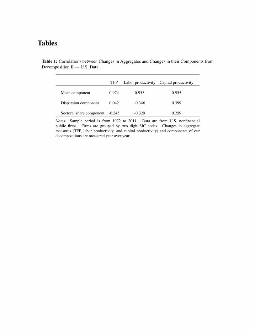
Tables
Table 1: Correlations between Changes in Aggregates and Changes in their Components fromDecomposition II — U.S. Data
TFP Labor productivity Capital productivity
Mean component 0.974 0.955 0.955
Dispersion component 0.042 -0.346 0.399
Sectoral share component -0.245 -0.329 0.259
Notes: Sample period is from 1972 to 2011. Data are from U.S. nonfinancialpublic firms. Firms are grouped by two digit SIC codes. Changes in aggregatemeasures (TFP, labor productivity, and capital productivity) and components of ourdecompositions are measured year over year.
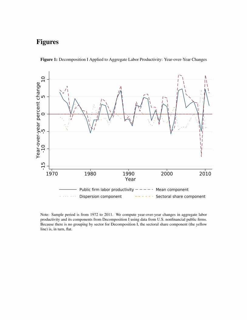
Figures
Figure 1: Decomposition I Applied to Aggregate Labor Productivity: Year-over-Year Changes
-15
-10
-50
510
Year
-ove
r-ye
ar p
erce
nt c
hang
e
1970 1980 1990 2000 2010Year
Public firm labor productivity Mean componentDispersion component Sectoral share component
Note: Sample period is from 1972 to 2011. We compute year-over-year changes in aggregate laborproductivity and its components from Decomposition I using data from U.S. nonfinancial public firms.Because there is no grouping by sector for Decomposition I, the sectoral share component (the yellowline) is, in turn, flat.
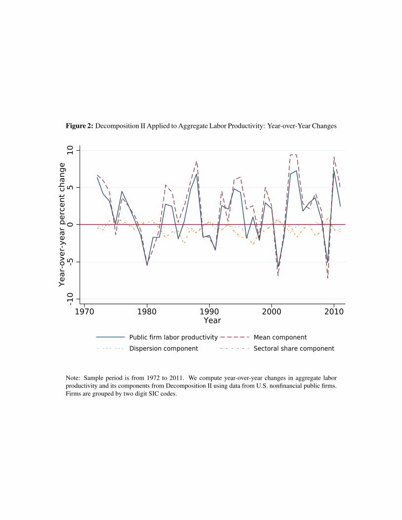
Figure 2: Decomposition II Applied to Aggregate Labor Productivity: Year-over-Year Changes
-10
-50
510
Year
-ove
r-ye
ar p
erce
nt c
hang
e
1970 1980 1990 2000 2010Year
Public firm labor productivity Mean componentDispersion component Sectoral share component
Note: Sample period is from 1972 to 2011. We compute year-over-year changes in aggregate laborproductivity and its components from Decomposition II using data from U.S. nonfinancial public firms.Firms are grouped by two digit SIC codes.
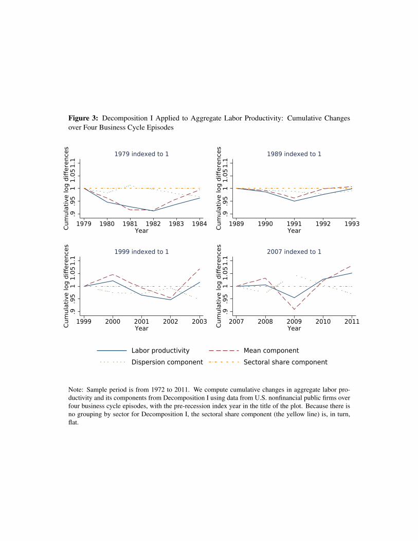
Figure 3: Decomposition I Applied to Aggregate Labor Productivity: Cumulative Changesover Four Business Cycle Episodes
.9.9
51
1.05
1.1
Cum
ulat
ive
log
diff
eren
ces
1979 1980 1981 1982 1983 1984Year
1979 indexed to 1
.9.9
51
1.05
1.1
Cum
ulat
ive
log
diff
eren
ces
1989 1990 1991 1992 1993Year
1989 indexed to 1
.9.9
51
1.05
1.1
Cum
ulat
ive
log
diff
eren
ces
1999 2000 2001 2002 2003Year
1999 indexed to 1
.9.9
51
1.05
1.1
Cum
ulat
ive
log
diff
eren
ces
2007 2008 2009 2010 2011Year
2007 indexed to 1
Labor productivity Mean componentDispersion component Sectoral share component
Note: Sample period is from 1972 to 2011. We compute cumulative changes in aggregate labor pro-ductivity and its components from Decomposition I using data from U.S. nonfinancial public firms overfour business cycle episodes, with the pre-recession index year in the title of the plot. Because there isno grouping by sector for Decomposition I, the sectoral share component (the yellow line) is, in turn,flat.

Figure 4: Decomposition II Applied to Aggregate Labor Productivity: Cumulative Changesover Four Business Cycle Episodes
.9.9
51
1.05
1.1
Cum
ulat
ive
log
diff
eren
ces
1979 1980 1981 1982 1983 1984Year
1979 indexed to 1
.9.9
51
1.05
1.1
Cum
ulat
ive
log
diff
eren
ces
1989 1990 1991 1992 1993Year
1989 indexed to 1
.9.9
51
1.05
1.1
Cum
ulat
ive
log
diff
eren
ces
1999 2000 2001 2002 2003Year
1999 indexed to 1
.9.9
51
1.05
1.1
Cum
ulat
ive
log
diff
eren
ces
2007 2008 2009 2010 2011Year
2007 indexed to 1
Labor productivity Mean componentDispersion component Sectoral share component
Note: Sample period is from 1972 to 2011. We compute cumulative changes in aggregate labor pro-ductivity and its components from Decomposition I using data from U.S. nonfinancial public firms overfour business cycle episodes, with the pre-recession index year in the title of the plot. Firms are groupedby two digit SIC codes.
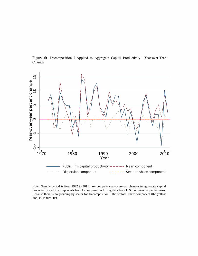
Figure 5: Decomposition I Applied to Aggregate Capital Productivity: Year-over-YearChanges
-10
-50
510
15Ye
ar-o
ver-
year
per
cent
cha
nge
1970 1980 1990 2000 2010Year
Public firm capital productivity Mean componentDispersion component Sectoral share component
Note: Sample period is from 1972 to 2011. We compute year-over-year changes in aggregate capitalproductivity and its components from Decomposition I using data from U.S. nonfinancial public firms.Because there is no grouping by sector for Decomposition I, the sectoral share component (the yellowline) is, in turn, flat.
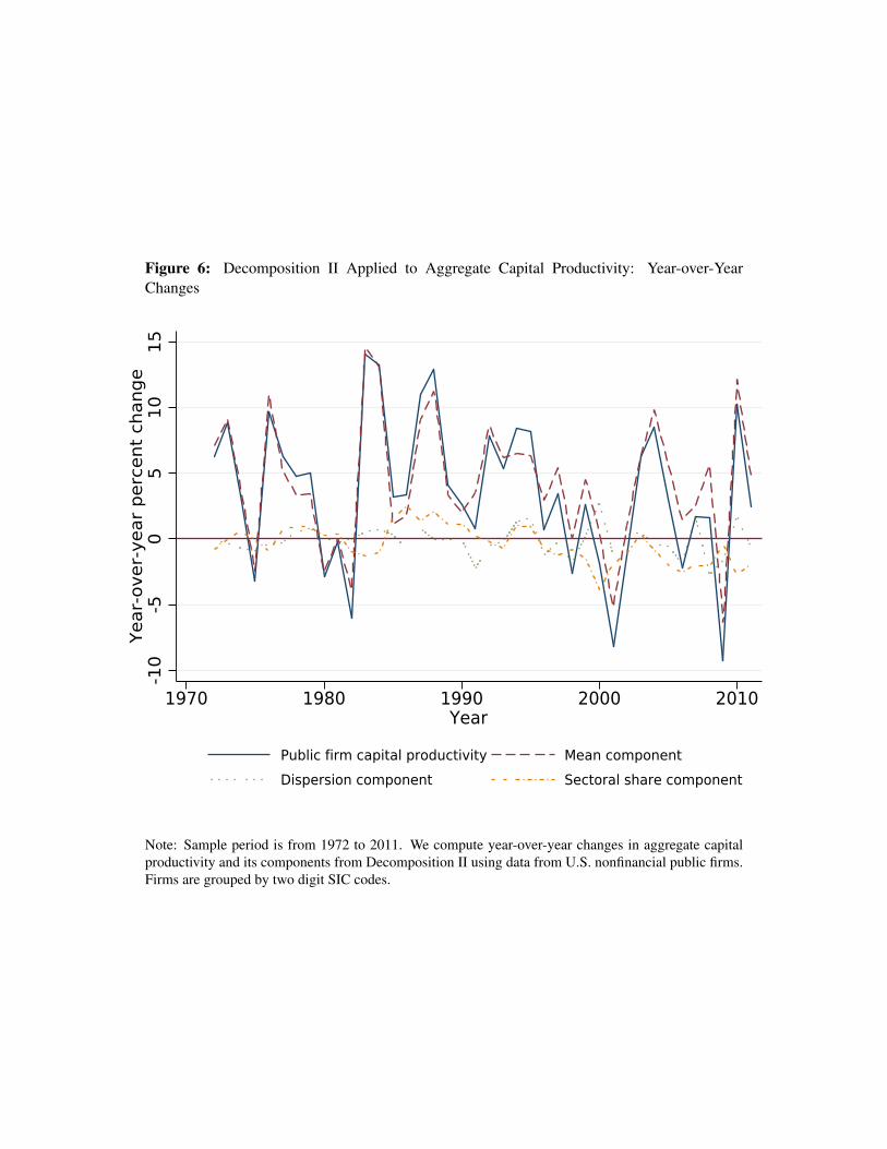
Figure 6: Decomposition II Applied to Aggregate Capital Productivity: Year-over-YearChanges
-10
-50
510
15Ye
ar-o
ver-
year
per
cent
cha
nge
1970 1980 1990 2000 2010Year
Public firm capital productivity Mean componentDispersion component Sectoral share component
Note: Sample period is from 1972 to 2011. We compute year-over-year changes in aggregate capitalproductivity and its components from Decomposition II using data from U.S. nonfinancial public firms.Firms are grouped by two digit SIC codes.
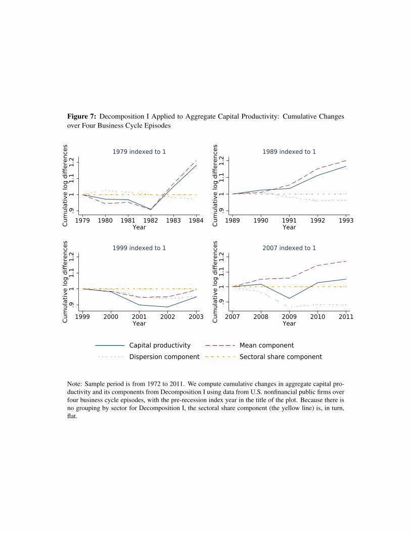
Figure 7: Decomposition I Applied to Aggregate Capital Productivity: Cumulative Changesover Four Business Cycle Episodes
.91
1.1
1.2
Cum
ulat
ive
log
diff
eren
ces
1979 1980 1981 1982 1983 1984Year
1979 indexed to 1
.91
1.1
1.2
Cum
ulat
ive
log
diff
eren
ces
1989 1990 1991 1992 1993Year
1989 indexed to 1
.91
1.1
1.2
Cum
ulat
ive
log
diff
eren
ces
1999 2000 2001 2002 2003Year
1999 indexed to 1
.91
1.1
1.2
Cum
ulat
ive
log
diff
eren
ces
2007 2008 2009 2010 2011Year
2007 indexed to 1
Capital productivity Mean componentDispersion component Sectoral share component
Note: Sample period is from 1972 to 2011. We compute cumulative changes in aggregate capital pro-ductivity and its components from Decomposition I using data from U.S. nonfinancial public firms overfour business cycle episodes, with the pre-recession index year in the title of the plot. Because there isno grouping by sector for Decomposition I, the sectoral share component (the yellow line) is, in turn,flat.
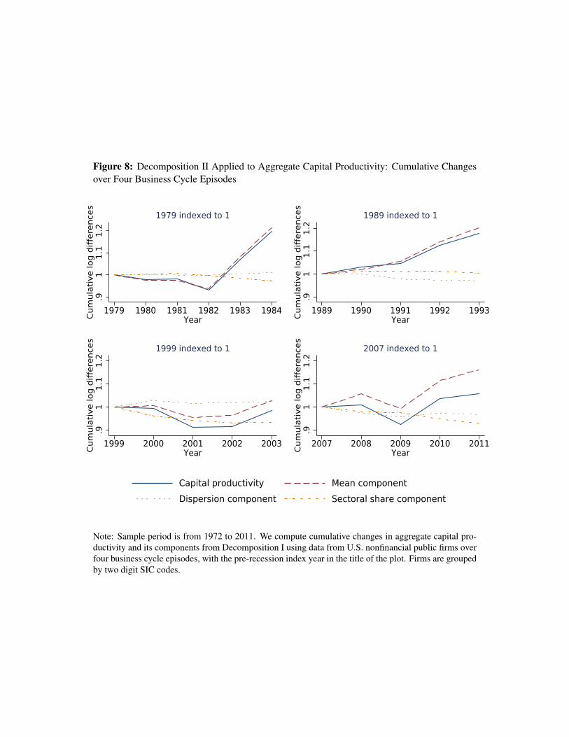
Figure 8: Decomposition II Applied to Aggregate Capital Productivity: Cumulative Changesover Four Business Cycle Episodes
.91
1.1
1.2
Cum
ulat
ive
log
diff
eren
ces
1979 1980 1981 1982 1983 1984Year
1979 indexed to 1
.91
1.1
1.2
Cum
ulat
ive
log
diff
eren
ces
1989 1990 1991 1992 1993Year
1989 indexed to 1
.91
1.1
1.2
Cum
ulat
ive
log
diff
eren
ces
1999 2000 2001 2002 2003Year
1999 indexed to 1
.91
1.1
1.2
Cum
ulat
ive
log
diff
eren
ces
2007 2008 2009 2010 2011Year
2007 indexed to 1
Capital productivity Mean componentDispersion component Sectoral share component
Note: Sample period is from 1972 to 2011. We compute cumulative changes in aggregate capital pro-ductivity and its components from Decomposition I using data from U.S. nonfinancial public firms overfour business cycle episodes, with the pre-recession index year in the title of the plot. Firms are groupedby two digit SIC codes.
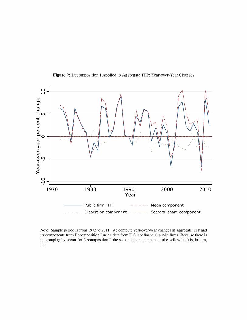
Figure 9: Decomposition I Applied to Aggregate TFP: Year-over-Year Changes
-10
-50
510
Year
-ove
r-ye
ar p
erce
nt c
hang
e
1970 1980 1990 2000 2010Year
Public firm TFP Mean componentDispersion component Sectoral share component
Note: Sample period is from 1972 to 2011. We compute year-over-year changes in aggregate TFP andits components from Decomposition I using data from U.S. nonfinancial public firms. Because there isno grouping by sector for Decomposition I, the sectoral share component (the yellow line) is, in turn,flat.
Figure 10: Decomposition II Applied to Aggregate TFP: Year-over-Year Changes
-50
510
Year
-ove
r-ye
ar p
erce
nt c
hang
e
1970 1980 1990 2000 2010Year
Public firm TFP Mean componentDispersion component Sectoral share component
Note: Sample period is from 1972 to 2011. We compute year-over-year changes in aggregate TFP and itscomponents from Decomposition II using data from U.S. nonfinancial public firms. Firms are groupedby two digit SIC codes.
Figure 11: Decomposition I Applied to Aggregate TFP: Cumulative Changes over Four Busi-ness Cycle Episodes
.9.9
51
1.05
1.1
Cum
ulat
ive
log
diff
eren
ces
1979 1980 1981 1982 1983 1984Year
1979 indexed to 1
.9.9
51
1.05
1.1
Cum
ulat
ive
log
diff
eren
ces
1989 1990 1991 1992 1993Year
1989 indexed to 1
.9.9
51
1.05
1.1
Cum
ulat
ive
log
diff
eren
ces
1999 2000 2001 2002 2003Year
1999 indexed to 1
.9.9
51
1.05
1.1
Cum
ulat
ive
log
diff
eren
ces
2007 2008 2009 2010 2011Year
2007 indexed to 1
TFP Mean componentDispersion component Sectoral share component
Note: Sample period is from 1972 to 2011. We compute cumulative changes in aggregate TFP and itscomponents from Decomposition I using data from U.S. nonfinancial public firms over four businesscycle episodes, with the pre-recession index year in the title of the plot. Because there is no grouping bysector for Decomposition I, the sectoral share component (the yellow line) is, in turn, flat.
Figure 12: Decomposition II Applied to Aggregate TFP: Cumulative Changes over Four Busi-ness Cycle Episodes
.9.9
51
1.05
1.1
Cum
ulat
ive
log
diff
eren
ces
1979 1980 1981 1982 1983 1984Year
1979 indexed to 1
.9.9
51
1.05
1.1
Cum
ulat
ive
log
diff
eren
ces
1989 1990 1991 1992 1993Year
1989 indexed to 1
.9.9
51
1.05
1.1
Cum
ulat
ive
log
diff
eren
ces
1999 2000 2001 2002 2003Year
1999 indexed to 1
.9.9
51
1.05
1.1
Cum
ulat
ive
log
diff
eren
ces
2007 2008 2009 2010 2011Year
2007 indexed to 1
TFP Mean componentDispersion component Sectoral share component
Note: Sample period is from 1972 to 2011. We compute cumulative changes in aggregate TFP and itscomponents from Decomposition I using data from U.S. nonfinancial public firms over four businesscycle episodes, with the pre-recession index year in the title of the plot. Firms are grouped by two digitSIC codes.
Figure 13: Decomposition I Applied to Aggregate TFP: Year-over-Year Changes
-10
-50
510
Year
-ove
r-ye
ar p
erce
nt c
hang
e
2000 2005 2010Year
Public firm TFP Mean componentDispersion component Sectoral share component
Note: Sample period is from 1972 to 2011. We compute year-over-year changes in aggregate TFP andits components from Decomposition I using data from Japanese nonfinancial public firms. Because thereis no grouping by sector for Decomposition I, the sectoral share component (the yellow line) is, in turn,flat.
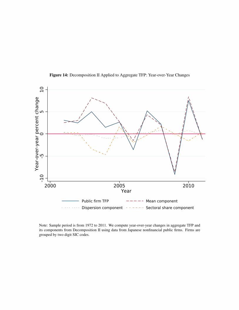
Figure 14: Decomposition II Applied to Aggregate TFP: Year-over-Year Changes
-10
-50
510
Year
-ove
r-ye
ar p
erce
nt c
hang
e
2000 2005 2010Year
Public firm TFP Mean componentDispersion component Sectoral share component
Note: Sample period is from 1972 to 2011. We compute year-over-year changes in aggregate TFP andits components from Decomposition II using data from Japanese nonfinancial public firms. Firms aregrouped by two digit SIC codes.
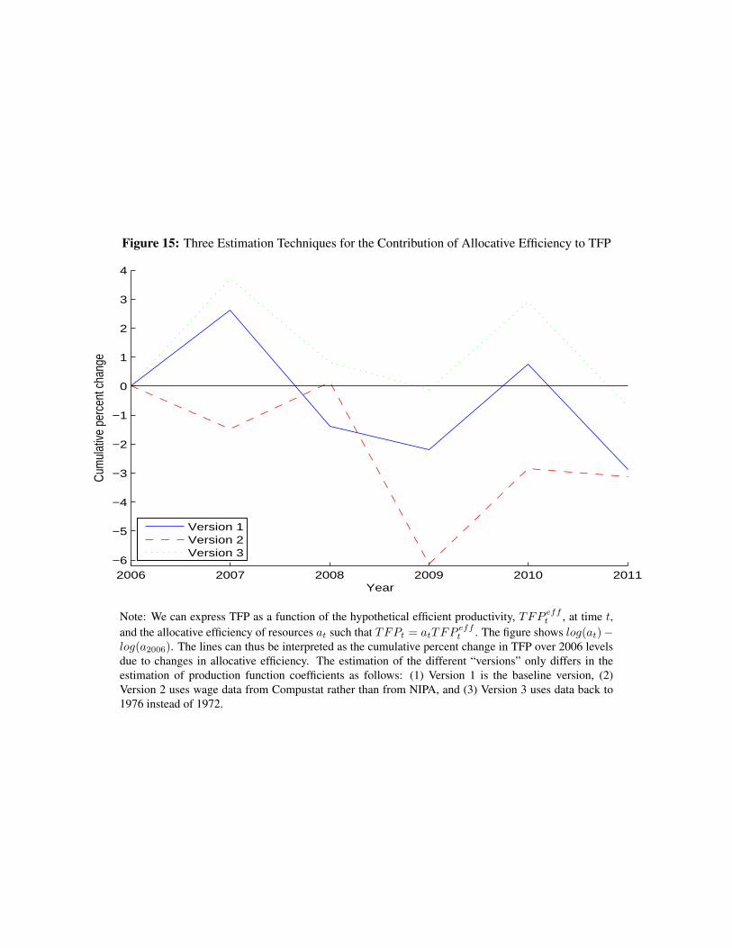
Figure 15: Three Estimation Techniques for the Contribution of Allocative Efficiency to TFP
2006 2007 2008 2009 2010 2011−6
−5
−4
−3
−2
−1
0
1
2
3
4
Year
Cum
ulat
ive
perc
ent c
hang
e
Version 1Version 2Version 3
Note: We can express TFP as a function of the hypothetical efficient productivity, TFP efft , at time t,and the allocative efficiency of resources at such that TFPt = atTFP
efft . The figure shows log(at)−
log(a2006). The lines can thus be interpreted as the cumulative percent change in TFP over 2006 levelsdue to changes in allocative efficiency. The estimation of the different “versions” only differs in theestimation of production function coefficients as follows: (1) Version 1 is the baseline version, (2)Version 2 uses wage data from Compustat rather than from NIPA, and (3) Version 3 uses data back to1976 instead of 1972.
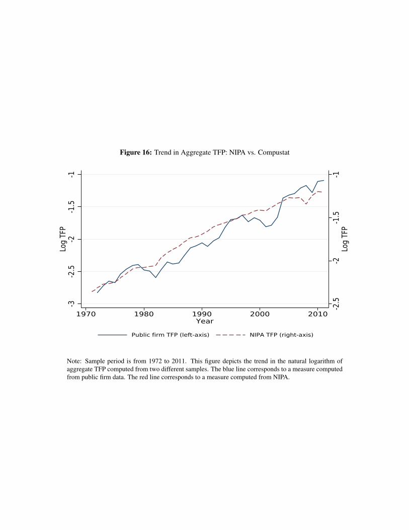
Figure 16: Trend in Aggregate TFP: NIPA vs. Compustat
-2.5
-2-1
.5-1
Log
TFP
-3-2
.5-2
-1.5
-1Lo
g TF
P
1970 1980 1990 2000 2010Year
Public firm TFP (left-axis) NIPA TFP (right-axis)
Note: Sample period is from 1972 to 2011. This figure depicts the trend in the natural logarithm ofaggregate TFP computed from two different samples. The blue line corresponds to a measure computedfrom public firm data. The red line corresponds to a measure computed from NIPA.
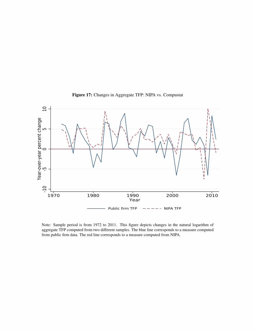
Figure 17: Changes in Aggregate TFP: NIPA vs. Compustat
-10
-50
510
Year
-ove
r-yea
r per
cent
cha
nge
1970 1980 1990 2000 2010Year
Public firm TFP NIPA TFP
Note: Sample period is from 1972 to 2011. This figure depicts changes in the natural logarithm ofaggregate TFP computed from two different samples. The blue line corresponds to a measure computedfrom public firm data. The red line corresponds to a measure computed from NIPA.
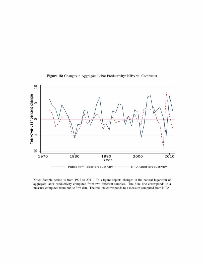
Figure 18: Changes in Aggregate Labor Productivity: NIPA vs. Compustat
-10
-50
510
Year
-ove
r-yea
r per
cent
cha
nge
1970 1980 1990 2000 2010Year
Public firm labor productivity NIPA labor productivity
Note: Sample period is from 1972 to 2011. This figure depicts changes in the natural logarithm ofaggregate labor productivity computed from two different samples. The blue line corresponds to ameasure computed from public firm data. The red line corresponds to a measure computed from NIPA.
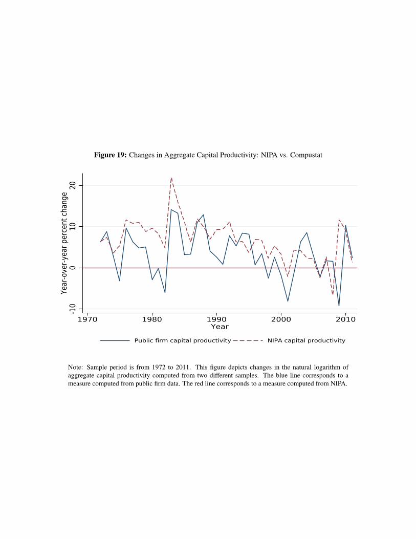
Figure 19: Changes in Aggregate Capital Productivity: NIPA vs. Compustat
-10
010
20Ye
ar-o
ver-y
ear p
erce
nt c
hang
e
1970 1980 1990 2000 2010Year
Public firm capital productivity NIPA capital productivity
Note: Sample period is from 1972 to 2011. This figure depicts changes in the natural logarithm ofaggregate capital productivity computed from two different samples. The blue line corresponds to ameasure computed from public firm data. The red line corresponds to a measure computed from NIPA.