Embed Size (px)
Citation preview

Access Control in XML PDMS Query Answering
by
Shuan Wang
B.Sc., Beijing Normal University, P.R. China, 2001M.Sc., Peking University, P.R. China, 2004
A THESIS SUBMITTED IN PARTIAL FULFILMENT OFTHE REQUIREMENTS FOR THE DEGREE OF
Master of Science
in
The Faculty of Graduate Studies
(Computer Science)
The University Of British Columbia
February 14, 2007
c© Shuan Wang 2007
Abstract
Peer data management system (PDMS) is a decentralized system, in which each
peer is autonomous and has its own schema and database. With the help of
pairwise schema mapping built between any two relevant peers, a query at one
peer can be rewritten and broadcast to the whole PDMS. Then answers from
multiple peers are returned to the querying peer. In our thesis, we exploit
the access control issues in the query-answering process of the XML PDMS.
We propose a formal syntax for access control policy (ACP) to specify the
fine-grained access control privileges on peers’ local XML database. We also
design several query-answering algorithms that aim to handle access control
in the PDMS, define the algorithm properties of Information Leakage Free and
Completeness, and analyze every designed query-answering algorithm on the two
properties. A comprehensive cost model, which consists of the major tasks and
primitive operations, is proposed by us to assess the query-answering algorithms.
We implement the designed query-answering algorithms, compare their running
time, and test the scalability in different facets.
ii
Table of Contents
Abstract . . . . . . . . . . . . . . . . . . . . . . . . . . . . . . . . . . . ii
Table of Contents . . . . . . . . . . . . . . . . . . . . . . . . . . . . . . iii
List of Tables . . . . . . . . . . . . . . . . . . . . . . . . . . . . . . . . vi
List of Figures . . . . . . . . . . . . . . . . . . . . . . . . . . . . . . . . vii
Acknowledgements . . . . . . . . . . . . . . . . . . . . . . . . . . . . . ix
1 Introduction . . . . . . . . . . . . . . . . . . . . . . . . . . . . . . . 1
1.1 Background . . . . . . . . . . . . . . . . . . . . . . . . . . . . . . 1
1.2 Motivation and Challenges . . . . . . . . . . . . . . . . . . . . . . 4
1.3 Problem Statement . . . . . . . . . . . . . . . . . . . . . . . . . . 6
1.4 Contributions . . . . . . . . . . . . . . . . . . . . . . . . . . . . . 7
1.5 Thesis Outline . . . . . . . . . . . . . . . . . . . . . . . . . . . . 7
2 Related Work . . . . . . . . . . . . . . . . . . . . . . . . . . . . . . . 9
2.1 Peer Data Management System (PDMS) . . . . . . . . . . . . . . 9
2.2 Query Containment . . . . . . . . . . . . . . . . . . . . . . . . . 12
2.3 Access Control on XML Documents . . . . . . . . . . . . . . . . 14
3 Access Control in XML PDMS . . . . . . . . . . . . . . . . . . . 16
3.1 The Problem in General . . . . . . . . . . . . . . . . . . . . . . . 16
3.1.1 General Sense of Information Leakage and Completeness . 17
3.1.2 General Methods of Access Control . . . . . . . . . . . . . 17
3.1.3 Example . . . . . . . . . . . . . . . . . . . . . . . . . . . . 19
3.2 Access Control Policy (ACP) Formal Definition . . . . . . . . . . 20
3.3 PDMS Scenarios with ACP Examples . . . . . . . . . . . . . . . 22
3.4 Semantics of PDMS Query-Answering under ACPs . . . . . . . . 28
iii
Table of Contents
4 Strategies and Options for the Query-Answering Process . . . 30
4.1 Intuition . . . . . . . . . . . . . . . . . . . . . . . . . . . . . . . . 30
4.2 Formal Definitions for Strategy and Option . . . . . . . . . . . . 32
4.3 Basic Assumptions . . . . . . . . . . . . . . . . . . . . . . . . . . 33
4.4 Strategies and Options Designed . . . . . . . . . . . . . . . . . . 35
5 Information Leakage and Completeness for (S,O) Pairs . . . . 40
5.1 Information Leakage (IL) . . . . . . . . . . . . . . . . . . . . . . 40
5.1.1 Definitions . . . . . . . . . . . . . . . . . . . . . . . . . . 40
5.1.2 The Sufficient and Necessary Condition for IL-Free . . . . 42
5.1.3 IL-Free Analysis for all (S,O) pairs . . . . . . . . . . . . . 43
5.2 Completeness . . . . . . . . . . . . . . . . . . . . . . . . . . . . . 46
5.2.1 Definitions . . . . . . . . . . . . . . . . . . . . . . . . . . 46
5.2.2 The Sufficient and Necessary Condition for Completeness 48
5.2.3 Completeness Analysis for all (S,O) pairs . . . . . . . . . 50
6 Cost Analysis for (S,O) pairs . . . . . . . . . . . . . . . . . . . . . 54
6.1 The Cost Model . . . . . . . . . . . . . . . . . . . . . . . . . . . 54
6.2 Cost Analysis Result . . . . . . . . . . . . . . . . . . . . . . . . . 59
6.2.1 Query Transmitting Cost . . . . . . . . . . . . . . . . . . 60
6.2.2 Query Rewriting Cost . . . . . . . . . . . . . . . . . . . . 60
6.2.3 ACP Evaluation Cost . . . . . . . . . . . . . . . . . . . . 61
6.2.4 Answer Routing Cost . . . . . . . . . . . . . . . . . . . . 62
6.2.5 ACP Distributing Cost . . . . . . . . . . . . . . . . . . . 64
6.2.6 Annotating Cost . . . . . . . . . . . . . . . . . . . . . . . 65
6.2.7 Annotation Shipping Cost . . . . . . . . . . . . . . . . . . 66
6.3 Hypothesis for Best (S,O) pairs . . . . . . . . . . . . . . . . . . . 67
7 Algorithm Details . . . . . . . . . . . . . . . . . . . . . . . . . . . . 69
7.1 Algorithm for Query-Rewriting in light of ACPs . . . . . . . . . 69
7.1.1 Algorithm Description . . . . . . . . . . . . . . . . . . . . 69
7.1.2 Example . . . . . . . . . . . . . . . . . . . . . . . . . . . . 70
7.2 Algorithms for O3 . . . . . . . . . . . . . . . . . . . . . . . . . . 75
7.2.1 Safe-Peer-List Finding Algorithm . . . . . . . . . . . . . . 75
7.2.2 Answer Routing Algorithm . . . . . . . . . . . . . . . . . 76
7.3 Algorithms for Option 5 . . . . . . . . . . . . . . . . . . . . . . . 80
7.3.1 Partitioning Semantics and Methodologies . . . . . . . . . 80
iv
Table of Contents
7.3.2 Data-level Partitioning Algorithm . . . . . . . . . . . . . 81
7.3.3 Schema-level Partitioning Algorithm . . . . . . . . . . . . 82
8 Experimental Study . . . . . . . . . . . . . . . . . . . . . . . . . . . 86
8.1 Experimental Settings and Implementation . . . . . . . . . . . . 86
8.2 (S, O) Pair Comparison and Analysis . . . . . . . . . . . . . . . . 87
8.3 Scalability Results and Analysis . . . . . . . . . . . . . . . . . . . 91
9 Conclusions and Future Work . . . . . . . . . . . . . . . . . . . . 97
Bibliography . . . . . . . . . . . . . . . . . . . . . . . . . . . . . . . . . 99
v
List of Tables
5.1 IL-free Result Matrix . . . . . . . . . . . . . . . . . . . . . . . . . 43
5.2 Completeness II Result Matrix . . . . . . . . . . . . . . . . . . . 50
6.1 Query Transmitting Cost (unit: query-hop) . . . . . . . . . . . . 60
6.2 Query Rewriting Cost (unit: qrewrite-acp) . . . . . . . . . . . . . 61
6.3 ACP Evaluation Cost (unit: acp-eval) . . . . . . . . . . . . . . . 61
6.4 Answer Routing Cost (unit: tuple-hop) . . . . . . . . . . . . . . . 63
6.5 ACP Distributing Cost (unit: acp-hop) . . . . . . . . . . . . . . . 64
6.6 Annotating Cost (unit: annot-update) . . . . . . . . . . . . . . . 65
6.7 Annotation Shipping Cost (unit: annot-hop) . . . . . . . . . . . 66
vi
List of Figures
1.1 A Simple PDMS Example . . . . . . . . . . . . . . . . . . . . . . 2
1.2 Motivation Example for Access Control in an XML PDMS . . . . 5
2.1 Data Integration System Example . . . . . . . . . . . . . . . . . 10
2.2 PDMS Example . . . . . . . . . . . . . . . . . . . . . . . . . . . . 10
3.1 Example for General Methods of Access Control . . . . . . . . . 19
3.2 Hospital PDMS Example . . . . . . . . . . . . . . . . . . . . . . 22
3.3 Conference Example . . . . . . . . . . . . . . . . . . . . . . . . . 24
3.4 Company Management PDMS Example . . . . . . . . . . . . . . 26
3.5 Example for Semantics of PDMS Query Answering under ACPs . 29
5.1 Problem in Completeness I (Ideal Completeness) . . . . . . . . . 47
7.1 Query-Rewriting in light of ACP Algorithm . . . . . . . . . . . . 71
7.2 Example for Safe-Peer-List Finding Algorithm . . . . . . . . . . . 75
7.3 Safe-Peer-List Finding Algorithm . . . . . . . . . . . . . . . . . . 77
7.4 Example for O3 Answer Routing Algorithm . . . . . . . . . . . . 78
7.5 O3 Answer Routing Algorithm . . . . . . . . . . . . . . . . . . . 79
7.6 Answer Partitioning Semantics . . . . . . . . . . . . . . . . . . . 80
7.7 Data-level Partitioning Algorithm . . . . . . . . . . . . . . . . . . 83
7.8 Schema-level Partitioning Algorithm . . . . . . . . . . . . . . . . 85
8.1 Running Time Comparison of (S, O) Pairs, in case of Large Net-
work Latency . . . . . . . . . . . . . . . . . . . . . . . . . . . . . 89
8.2 Running Time Comparison of (S, O) Pairs, in case of Small Net-
work Latency . . . . . . . . . . . . . . . . . . . . . . . . . . . . . 90
8.3 Running Time Comparison of (S, O) Pairs. Under this experi-
ment setting, the PDMS topology and ACP distribution benefit
O3 finding a short answer-routing path, but doesn’t benefit O2A. 92
vii
List of Figures
8.4 the Running Time of the Query-Answering Process V.S. the Database
Size of the Target Peer for Each Compared (S, O) Pair. The net-
work latency is 100 ms. . . . . . . . . . . . . . . . . . . . . . . . 93
8.5 the Running Time of the Query-Answering Process V.S. the Database
Size of the Target Peer for (S1, O1). The network latency is 1000
ms. . . . . . . . . . . . . . . . . . . . . . . . . . . . . . . . . . . . 94
8.6 the Running Time of the Query-Answering Process V.S. the Num-
ber of ACPs per Peer for Each Compared (S, O) Pair . . . . . . . 95
8.7 the Running Time of the Query-Answering Process V.S. the Num-
ber of ACPs per Peer for (S1, O1), with the Network Latency of
0 ms, 100 ms and 200 ms Separately . . . . . . . . . . . . . . . . 95
8.8 the Running Time of the Query-Answering Process V.S. the Length
of the Longest Path from Source Peer to Target Peer for (S1, O1).
The experiment is done for both a PDMS with 20 peers and a
PDMS with 30 peers. . . . . . . . . . . . . . . . . . . . . . . . . . 96
viii
Acknowledgements
I would like to thank all the people who gave me support and help throughout
my degree.
First of all, I would like to thank my supervisors, Professor Laks V.S. Lak-
shmanan and Professor Rachel Pottinger, for their patient guidance and en-
couragement in my research work at UBC. Laks introduced me into the area
of access control in XML PDMS, and taught me the approaches how to ex-
plore unknown questions and study them clearly. Rachel brought forth many
insightful ideas in our group discussion, guided my experiment study, and paid
great effort in modifying my thesis. They both helped me a lot in improving
my communication skills.
Second, I would like to thank Professor Alan Wagner for dedicating his time
and effort in reviewing my thesis.
Third, many thanks to all my colleges and friends for their friendly support,
especially to Jian Xu, Jie Zhao, Shaofeng Bu, Wendy Wang, Suling Yang, Xi-
aodong Zhou, Terence Ho. Thanks a lot to Holly Kwan for her kind help in my
everyday life as our lab secretary.
Last but certainly not least, I would like to thank my families for their
endless love and firm support.
ix
Chapter 1
Introduction
The peer data management system (PDMS) is emerging as a flexible distributed
data management architecture. Moreover, with the significant increase of web
data, XML is now used as the underlying data model of peers in a PDMS.
However, the existing PDMS research has paid little attention to the access
control requirement in each peer for its database, which might greatly affect
the query-answering process in a PDMS. The access control issues in an XML
PDMS will be explored in our thesis.
In this chapter, we first introduce the background knowledge of PDMS,
XML, and XML queries (Section 1.1), then motivate our work by a concrete
example (Section 1.2). Section 1.3 concisely states the access control problem
in an XML PMDS. Our main contributions are summarized in Section 1.4.
1.1 Background
In this section, we introduce the background knowledge of our work: peer data
management systems, XML and XML queries.
A peer data management system (PDMS) is a distributed database man-
agement system based on a peer-to-peer architecture. Each node in a PDMS is
called a peer. A peer is autonomous, has its own database and schema. A peer
can join and leave the PDMS dynamically. Unlike the data integration system,
there is no server playing the central-control role in a PDMS. If two peers are
considered to be similar, one of their administrators builds a mapping between
the database schemas of the two peers. Such peers are called acquaintances.
Thus, the topology of a PDMS is an arbitrary connected graph, in which each
edge is such a pairwise mapping. A query can be put forth at any peer. The
query is first evaluated at the peer’s local database, then it is passed to each of
its acquaintances. When the query is passed to each acquaintance, the mapping
is used to translate the query into a new query over the acquaintance’s schema.
Similarly, it is then passed to all acquaintances of all those acquaintances and
1

Chapter 1. Introduction
thus broadcast to the whole PDMS. Finally the answers at every relevant peer
is returned to the querying peer.
Figure 1.1: A Simple PDMS Example
As an illustration, Figure 1.1 shows a simple PDMS with four peers: Van-
couver General Hospital, Montreal General Hospital, Boston General Hospital,
and Toronto General Hospital. In this example, Toronto General Hospital is an
acquaintance of Boston General Hospital, so a mapping is built from Toronto
General Hospital Schema to Boston General Hospital Schema (the mapping is
denoted by an arrow from Toronto General Hospital Schema to Boston General
Hospital Schema). Similarly, other pairwise mapping are built between peers.
When a query Q is put forth at Toronto General Hospital, it is first evaluated
locally. Then Q is rewritten into Q′ according to the mapping from Toronto
General Hospital Schema to Boston General Hospital Schema. Q′ is sent to
Boston General Hospital and evaluated there. The answer of Q′ is routed back
to Toronto General Hospital. By this way, rewritten queries are broadcast in
the whole PDMS, and the answer from each hospital is returned to Toronto
General Hospital.
XML (eXtensible Markup Language) currently is the W3C recommendation
for publishing electronic data on the web. Nowadays, it is the de facto standard
for web documents and data storage. An XML document is plain text inter-
leaved with some markup, which divides the document content into character
data, container elements, and attributes of the elements. There is one and only
one root element in an XML document. Sub-elements are embedded within
an element. Thus, an XML document is modeled as a tree structure, in which
each node is an element or a character string. Normally, an XML document is
2
Chapter 1. Introduction
accompanied with an XML Schema, which fully specifies the structure and data
type information for this document. Therefore, XML can be used as databases
for peers in a PDMS. Mappings are built between schemas of XML databases
residing on acquaintances.
The standard query form for XML databases is XQuery. XPath is the main
functional structure of XQuery, and it is the syntax to accurately address parts
of an XML document. An XPath is a path expression for a sequence of steps
from one node to another node. In each step, there are three components: (1)
axis specifier: ‘/’ denotes child, ‘//’ denotes descendant, ‘@’ denotes attribute,
etc; (2) node test: ‘comment()’ denotes a comment node, ‘text()’ denotes the
text value of a node, etc; (3) predicate: a mathematic expression put in a square
bracket as a filter. Predefined operators can also be used in XPath, such as ‘|’
denoting the union of two node sets. As the first example, the XPath expres-
sion “publication//paper/*[@id=‘001’]” selects the element, whatever its name
(‘*’), if its id attribute value of ‘001’, who is a child (‘/’) of a paper element that
itself is a descendant (‘//’) of a publication element. As a more concrete ex-
ample, the Xpath expression “publication//paper[/author/text()=‘Rachel Pot-
tinger’]” selects the paper element, if it is a descendant (‘//’) of a publication
element and has an author child element (‘/’) whose text content (‘text()’) is
Rachel Pottinger. This Xpath expression retrieves the full paper list for Rachel
Pottinger. XPath queries can be categorized into several fragments according
to whether including ‘/’, ‘//’, ‘[ ]’,‘*’, ‘|’, Schema or DTD (another type of
XML schema). In this thesis, we concentrate on the XPath fragment
only with ‘/’, ‘//’, ‘[ ]’. For instance, our second XPath example “publi-
cation//paper[/author/text()=‘Rachel Pottinger’]” belongs to this XPath frag-
ment.
The tree pattern is the key construct for modeling XPath. A tree pattern
includes two components: (1) a tree, in which the nodes are labeled with vari-
ables, (2) a set of formulas, which are constraints on the tree nodes and their
properties (i.e. tags, attributes, contents). The tree has two types of edges: pc
(parent-child) edges and ad (ancestor-descendant) edges, which correspond to
‘/’ and ‘//’ in XPath.
3
Chapter 1. Introduction
1.2 Motivation and Challenges
As a flexible data management environment, a peer data management system is
suitable for many applications, such as the public medical institutions, the inter-
national company management, and the insurance system, etc. For example, a
public medical institution environment may consist of several hospitals, health-
care centers, the Ministry of Health, and emergency units. Each institution is
independent, has its own database and share the data across the web. Quite
often these institutions need to collaborate. For instance, when a patient is
transferred between hospitals, the patient’s medical history needs to be shared.
Probably there is no global schema for all the hospitals, so a data integration
system does not help. A PDMS is useful at this time. With the help of the
pairwise schema mapping, the patient’s illness history can be easily transferred
from one hospital to another one. Furthermore, a query asking for one patient’s
information can be put forth at a peer and broadcast in the whole PDMS, and
results will be retrieved from every relevant peer.
Although the existing PDMS projects [13, 35, 37, 40] can handle the prob-
lems of schema mapping and query rewriting, they do not effectively take into
account the access control requirements of peers, i.e., all the data on each peer
is public for other peers. This is not true for a realistic application. Because
a peer is autonomous, it has the requirement to define access control privileges
on its database, i.e., which peers have the right to access a specific part of its
database. For example, a hospital may only allow other hospitals to access the
illness history of a patient, but forbid any institution to access the personal
information of a patient. Such access control requirements are so common in
today’s database management systems that they should not be ignored in a
realistic PDMS. When access control exists in a PDMS, security problems will
arise. The existing query-answering algorithm does not work well in this case.
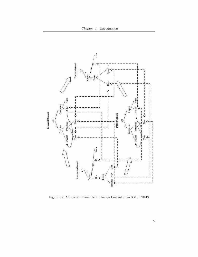
Let us observe a concrete example. It is shown in Figure 1.2. There are
four peers in the XML PDMS: Vancouver General Hospital, Montreal General
Hospital, Boston General Hospital and Toronto General Hospital. The schemas
for their XML databases are shown in the figure. The pairwise mappings of
their schemas are denoted by dash arrows. For simplicity, we call the four
peers Vancouver General Hospital, Montreal General Hospital, Toronto General
Hospital and Boston General Hospital separately as ‘vg’, ‘mg’, ‘tg’ and ‘bg’. And
the database residing on each peer is ‘vg.xml’ for ‘vg’, ‘mg.xml’ for ‘mg’, ‘tg.xml’
for ‘tg’, ‘bg.xml’ for ‘bg’. The possible message routing paths are denoted by
4
Chapter 1. Introduction
Figure 1.2: Motivation Example for Access Control in an XML PDMS
5

Chapter 1. Introduction
bold arrows.
Suppose a query “retrieve the illness history of Mary Smith” is put forth at
’vg’, rewritten according to schema mappings, and broadcast to the PDMS. Let
us treat ‘tg’ as the current answering peer. The rewritten query is evaluated on
‘tg.xml’ to get the ‘Event’ elements for Mary Smith. If ‘tg’ does not specify any
access control on its database, i.e. any peer can access all the data of ‘tg.xml’,
the answer can be routed back to ‘vg’ via either the path “tg → mg → vg” or
the path “tg → bg → vg”. This is the existing query-answering algorithm. The
case with access control may be different. Suppose in our scenario, ‘mg’ and
‘tg’ do not have a collaboration relationship such that ‘tg’ specifies the access
control of forbidding ‘mg’ to access any information on it. Thus, the answer for
the query “retrieve the illness history of Mary Smith” at ‘tg’ can not be routed
via the path “tg → mg → vg”. Otherwise, information leakage will arise, i.e.,
‘mg’ will see data that it is forbidden to access by ‘tg’. The answer can only
be routed via the path “tg → bg → vg”. From this example, we see that the
access control requirements of peers affect the PDMS query-answering process.
Furthermore, access control on a peer database can be more fine-grained and
complicated than the previous example, especially when XML is the data model.
What is the impact of access control on the PDMS query-answering process is
still unknown according to existing research work.
The major challenges we are faced with in a XML PDMS with access control
include: (1) How can we specify the access control requirement for a peer’s
XML database, which is fine-grained and expressive enough? (2) What is the
semantics of PMDS query-answering with access control? (3) What kind of
algorithms can be used for the PDMS query-answering process? (4) What is
the security property of these algorithms? (5) How to build a rational cost
model and assess the algorithms using this model? All these challenges will be
tackled in this thesis.
1.3 Problem Statement
A peer in a realistic peer data management system probably has access control
requirement on its own database. Therefore, a precise syntax for specifying
a access control requirement is necessary for an XML PDMS. Furthermore,
in a PDMS with access control, a naive query-answering algorithm no longer
works in terms of the security issue. Thus, new query-answering algorithms
6
Chapter 1. Introduction
need to be designed, theoretically ensuring no information leakage and other
good properties. A cost model is also required to assess any query-answering
algorithm for an XML PDMS.
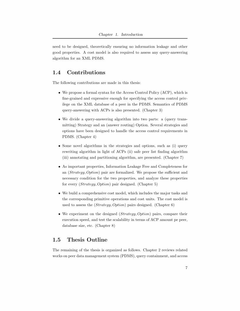
1.4 Contributions
The following contributions are made in this thesis:
• We propose a formal syntax for the Access Control Policy (ACP), which is
fine-grained and expressive enough for specifying the access control priv-
ilege on the XML database of a peer in the PDMS. Semantics of PDMS
query-answering with ACPs is also presented. (Chapter 3)
• We divide a query-answering algorithm into two parts: a (query trans-
mitting) Strategy and an (answer routing) Option. Several strategies and
options have been designed to handle the access control requirements in
PDMS. (Chapter 4)
• Some novel algorithms in the strategies and options, such as (i) query
rewriting algorithm in light of ACPs (ii) safe peer list finding algorithm
(iii) annotating and partitioning algorithm, are presented. (Chapter 7)
• As important properties, Information Leakage Free and Completeness for
an (Strategy, Option) pair are formalized. We propose the sufficient and
necessary condition for the two properties, and analyze these properties
for every (Strategy, Option) pair designed. (Chapter 5)
• We build a comprehensive cost model, which includes the major tasks and
the corresponding primitive operations and cost units. The cost model is
used to assess the (Strategy, Option) pairs designed. (Chapter 6)
• We experiment on the designed (Strategy, Option) pairs, compare their
execution speed, and test the scalability in terms of ACP amount pe peer,
database size, etc. (Chapter 8)
1.5 Thesis Outline
The remaining of the thesis is organized as follows. Chapter 2 reviews related
works on peer data management system (PDMS), query containment, and access
7
Chapter 1. Introduction
control on XML documents. In Chapter 3, we present the general access control
problem in the XML PDMS, the formal definition of Access Control Policy
(ACP), and the semantics of PDMS query-answering with ACPs. In Chapter 4,
we divide a query-answering algorithm into two parts – a strategy and an option.
Several strategies and options, which can handle access control, are also designed
there. Chapter 5 presents the formal definitions of IL-free and completeness, the
sufficient and necessary condition for each of them, and the analysis result for all
(Strategy, Option) pairs designed. In Chapter 6, we propose a comprehensive
cost model that is used to assess all (Strategy, Option) pairs. In Chapter 7,
some novel algorithms adopted in our strategies and options are elaborated
and illustrated in detail. Chapter 8 is the experimental study for algorithm
comparison, algorithm scalability, etc. Finally, our conclusions are stated in
Chapter 9, along with the future work.
8
Chapter 2
Related Work
As described in Chapter 1, the work of the thesis concentrates on the access
control scheme of the XML peer data management system. Peer data man-
agement system (PDMS) is the network environment we are working in; access
control is the main issue we are researching on; and query containment is a
necessary theoretical tool to design the query writing algorithm in the PDMS
query-answering process and to ensure the algorithm correctness.
Therefore, in this chapter we will summarize the previous research work on
peer data management system (Section 2.1), query containment (Section 2.2)
and access control on local XML documents (Section 2.3).
2.1 Peer Data Management System (PDMS)
Data integration systems have been researched and adopted in academia and
industry for a long time [5, 8, 16, 22, 28, 29, 30, 31]. They work well for sharing
information in a specific domain. However, data integration is faced with a big
problem: it requires to predefine a mediated schema before all nodes can share
information. Thus the mediated schema has become a bottleneck in a data
integration system.
Recently, the idea of a peer data management system (PDMS) [23] has
emerged as a step beyond data integration systems. A PDMS is a distributed
database management system based on a peer-to-peer architecture. In such
a system, each web node is an autonomous peer and has its local database
management system. The PDMS satisfies the need to have a decentralized,
loosely-coupled data management environment, in which any web node can
have different data model and contribute data, schema or mappings among
schemas. Unlike data integration systems, a PDMS does not require a central
control server or a global schema. Instead, mappings are constructed between
the schemas of any two related peers.
A simple example can help to understand the difference between data in-
9
Chapter 2. Related Work
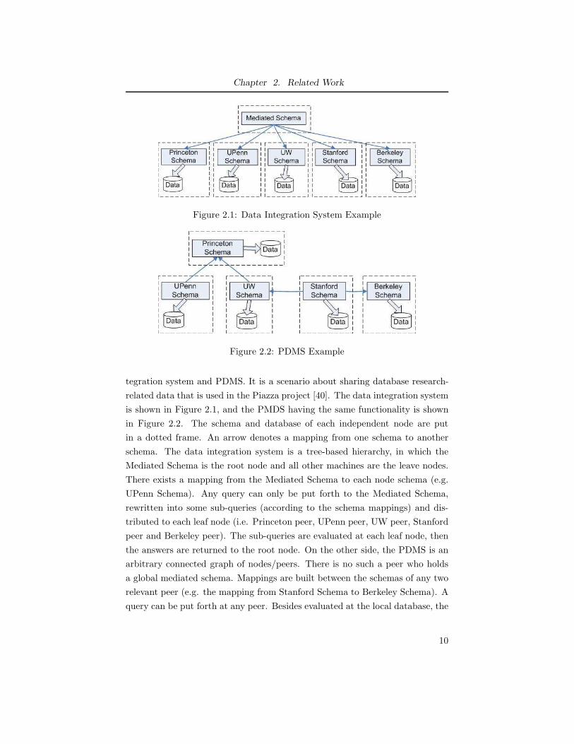
Figure 2.1: Data Integration System Example
Figure 2.2: PDMS Example
tegration system and PDMS. It is a scenario about sharing database research-
related data that is used in the Piazza project [40]. The data integration system
is shown in Figure 2.1, and the PMDS having the same functionality is shown
in Figure 2.2. The schema and database of each independent node are put
in a dotted frame. An arrow denotes a mapping from one schema to another
schema. The data integration system is a tree-based hierarchy, in which the
Mediated Schema is the root node and all other machines are the leave nodes.
There exists a mapping from the Mediated Schema to each node schema (e.g.
UPenn Schema). Any query can only be put forth to the Mediated Schema,
rewritten into some sub-queries (according to the schema mappings) and dis-
tributed to each leaf node (i.e. Princeton peer, UPenn peer, UW peer, Stanford
peer and Berkeley peer). The sub-queries are evaluated at each leaf node, then
the answers are returned to the root node. On the other side, the PDMS is an
arbitrary connected graph of nodes/peers. There is no such a peer who holds
a global mediated schema. Mappings are built between the schemas of any two
relevant peer (e.g. the mapping from Stanford Schema to Berkeley Schema). A
query can be put forth at any peer. Besides evaluated at the local database, the
10
Chapter 2. Related Work
query is rewritten into new queries with the help of the schema mappings and
broadcast in the PDMS. Answers from every peer will be returned to the query-
ing peer. For example, if a query Q is put forth at Stanford peer, Q is firstly
evaluated at Stanford Database. Meanwhile, Q is rewritten into Q′ according to
the mapping from Stanford Schema to Berkeley Schema, sent to Berkeley peer
and evaluated there. Q is also rewritten into Q′′ and sent to UW peer. By this
way, the original query Q is broadcast in the whole PDMS. All answers will be
returned to Stanford peer in the end.
In the following, We will analyze some important PDMS projets.
Piazza [23, 24, 40] is a classic PDMS using XML as the peer data model. Be-
cause each peer may have a different schema, Piazza provides a pairwise schema
mapping language similar to XQuery[12] and a query reformation algorithm
for rewriting queries between peers. Piazza recognizes and motivates the access
control as an important problem for a PDMS, but the only solution to the prob-
lem is a description of general plans to use encryption to enforce security. The
details of this approach were left as future work.
The Hyperion project [37] is relational database-based PDMS. Hyperion
builds and manages the mapping tables between peers at run time. And both
schema-level and data-level mappings are supported. Hyperion’s emphasis is
query answering among heterogenous peers, and it doesn’t address access control
or security issues.
HePToX [13] is a PDMS prototype using XML as peers’ underlying databases.
Peers are heterogenous. HePToX emphasizes on semi-automatically generating
Datalog-like mapping rules and the efficient query translation algorithm. Access
control issue is not considered in HePToX.
PeerDB [35] is an interesting system. The underlying database for each
peer is a relational database system. However, there is no mapping between
peer schemas. Instead, PeerDB uses the Information Retrieval (IR) technique
to retrieve answers from different peers. Thus, PeerDB is a combination of
database and IR systems. No access control issue is discussed in PeerDB.
As a conclusion, we see that the existing typical PDMS systems have not
studied the access control problem, although some of them have recognized it
as an important issue for a realistic PDMS. That is the work we will exploit in
this thesis.
11
Chapter 2. Related Work
2.2 Query Containment
As we mentioned at the beginning of this chapter, query containment will be
used as a theoretical tool to design our query rewriting algorithm in the PDMS
query-answering process. Intuitively speaking, when a query Q is rewritten into
a new query Q′ in light of an access control rule R, it must ensure that the
answer of Q′ is contained by both the answer of Q and the answer of R. That
is why query containment is important for our work.
Query containment problem was firstly exploited for conjunctive queries.
Conjunctive Query (CQ) is put forth by A.K. Chandra and P.M. Merlin [15]. A
Conjunctive Query is defined as a datalog rule H ← G1, ..., Gn, where H is
the head, the right side hand is the body and Gi(i = 1..n) are relations, which
are referred to as subgoals. The answer for a conjunctive query Q evaluated on
a relational database D is denoted as Q(D). In more details, Q(D) is the set
of the head got by performing a possible value substitution for variables in Q,
where the substitution turns every subgoal of Q’s body into a tuple in D.
Example 2.1 p(X, Y ) ← a(X, W ), b(W, Z), c(Z, Y ) is a conjunctive query Q.
Specifically, it states the following. The body describes the relations a, b, and
c. The re-use of variables indicates that the values must be the same. So the
body specifies that the second attribute of a must equal the first attribute of b,
and that the second attribute of b must equal the first attribute of c. For each
set of tuples that satisfy the body requirement, the head is instantiated. In this
case, a new tuple of relation p is created, and the attributes of p are given the
values of X and Y from the body. E.g., given a database D, there are three
relational tables a, b and c in it. In a, there is one tuple (x1, w1); In b, there
is one tuple (w1, z1); In c, there is one tuple (z1, y1). Then for the substitution
{X = x1, Y = y1, Z = z1, W = w1}, each subgoal in the body of Q is a tuple in
the database D. Thus, the instantiated head p(x1, y1) is in Q(D).
Give the definition of CQ and the meaning of a CQ evaluated on a database,
CQ Containment can be defined as:
Let Q1 and Q2 be two CQs. Q1 ⊆ Q2 iff ∀ database D: Q1(D) ⊆
Q2(D).
There are two classic approaches to test CQ containment: (1) containment
mapping, (2)canonical database. Containment Mapping can be defined as:
12
Chapter 2. Related Work
Q1 and Q2 are CQs, where Q1 : head1 ← sg1, ..., sgk and Q2 :
head2 ← SG1, ..., SGm. Then a containment mapping is a function
µ : vars(Q2) → vars(Q1) such that (1) µ(head2) = head1, (2)
∀i : µ(SGi) = sgj , for some j.
If Q1 and Q2 are CQs, then Q1 ⊆ Q2 iff ∃ a containment mapping µ : vars(Q2)→
vars(Q1).
Example 2.2 We have two CQ’s: Q1 : p(X, Z) ← a(X, W ), b(W, Z) and
Q2 : p(X, Z) ← a(X, W ), b(Y, Z). There exists a mapping µ from vars(Q2)
to vars(Q1): W → W , X → X, Y → W , Z → Z. µ makes the mapped
head of Q2 as p(X, Z), which equals the head of Q1. For Q2’s subgoals, we see
that µ(a(X, W )) = a(X, W ), which is a subgoal in Q1’s body, and µ(b(Y, Z)) =
b(W, Z), which is a subgoal in Q1’s body. Thus µ is a containment mapping
from Q2 to Q1, then Q1 ⊆ Q2.
Canonical Database method is to build a small number of databases D1,
..., Dn, such that Q1 ⊆ Q2 iff Q1(Di) ⊆ Q2(Di), where i = 1, ..., n. This method
is not used in our work, so we do not illustrate it here. For more details, please
refer to [41].
The CQ containment problem has been recognized as NP-complete in [15].
Much attention have been devoted to finding special classes of queries that ad-
mit polynomial time algorithms for containment and minimization[6, 7, 11, 17,
26, 27, 43].
With the popularity of XML query applications, query containment research
expands from CQs to XML queries. XQuery [12] is recognized as the XML
query standard. But it provides too many supportive structures, such as the
FLWOR expressions and constructors. To avoid being distracted by these sup-
portive structures, researchers have concentrated on XPath and its equivalent
representation Tree Pattern, which is the main functional structure of XQuery.
The concept and approaches for CQ containment have evolved to the work for
containment of XPath queries (or tree patterns). The difference of XPath con-
tainment from CQ containment is that the query structures are trees and the
queries may have recursions.
The semantics of XPath containment is exactly the same as that of CQ con-
tainment. Existing approaches for checking CQ containment work for XPath
query containment as well, but after some extension. The canonical model
13
Chapter 2. Related Work
(database) technique [19, 32, 33], the homomorphism (containment mapping)
technique [9, 20, 33, 36, 42] are widely used in the complexity analysis and al-
gorithm design of XPath containment. For example, homomorphism is formally
redefined for tree pattern containment in [20]:
“A homomorphism h from a pattern q to a pattern p is a total
mapping from the nodes of q to the nodes of p such that: (1) h pre-
serves node types (i.e. ∀u ∈ Nq : λq(u) 6=′ ∗′ ⇒ λq(u) = λp(h(u)),
where u is a node in q, Nq is the node set of q, and λ() is the func-
tion to find a node tag.); (2) h preserves structural relationships (i.e.
whenever v is a child (resp. descendant) of u in q, h(v) is a child
(resp. descendant) of h(u) in p).”
Checking query containment for many XPath fragments has been verified
to be extremely hard. Fortunately, for some XPath fragments we can still find
polynomial time algorithms. All the complexity results for containment of dif-
ferent XPath fragments are summarized in [38]. As mentioned in Section 1.1,
in the thesis we deal with an XPath fragment only with ‘/’, ‘//’, ‘[ ]’, which is
shown in [38] to have a polynomial time algorithm for finding a query contain-
ment. Most XPath expressions in usual XML queries fall into this fragment and
it is a good start for us to design algorithms for this XPath fragment.
2.3 Access Control on XML Documents
Access control in an XML PDMS is the main problem we are working on. It is
necessary for us to analyze the existing approaches for securing XML documents.
With the development of web-based applications, XML has become the de
facto standard of semi-structured data representation. It provides an easy way
to publish information. Selective distribution and sharing of XML documents
requires enforcement of access control. This ensures that specific information is
accessible only to authorized entities or roles.
Different access control approaches for local XML documents have been pro-
posed. Among them, access control policy model is widely recognized as an
expressive, fine-grained method. An Access Control Policy is a rule defined
to permit or deny the use of some objects/elements in an XML document by a
subject/user.
XACML[39] presents an XML schema for specifying access control policies
on XML documents. However, it is very complicated and even requires a spe-
14
Chapter 2. Related Work
cific processing model to interpret the access control policies. Paper [25] defines
an access control language using the concept of role, which is an abstract repre-
sentation of a set of privileges and could be assigned to users. It supports both
read/write and positive/negative policies. Paper [21] formalizes access control
policies in a SQL security model compatible manner, but it doesn’t support
negative policies. For all these work, the permission/prohibition on an element
is automatically propagated to its subelements. The above work concentrate on
the formal expression of an access control policy, not on its usage.
Access control policies can also be manipulated in different ways. The
method of [18] is view-based. It allows the definition and enforcement of ac-
cess control directly on XML documents, then produces a separate view on the
document for each user. The method of [10, 34] are encryption-based. They de-
fine a formal syntax of access control policies for XML documents, and encrypt
different portions of the same document according to different encryption keys.
Then various users can use their own encryption keys to get the desired portion
of the same encrypted document. Paper [14] is the first step to handle query-
ing XML data in light of access control policies. Its access control policies are
XML-compatible. But only very simple XQuries can be transformed to directly
incorporate restrictions of access control policies on XQuery variables.
In later chapters, we will see that our access control policy model supports
both read/write and positive/negative privileges, and it plays an important role
in the query rewriting algorithm.
15
Chapter 3
Access Control in XML
PDMS
In Section 2.3, we have summarized the work of access control on local XML
documents. However, the existing research work does not reveal what problems
will arise in a PDMS, where access control on distributed XML data sources are
required.
In Section 3.1, we describe a general view of the access control problems in
a PDMS. Then we concentrate on our solution – Access Control Policy (ACP)
in the XML PDMS. We present the ACP formal syntax in Section 3.2, the ACP
examples in Section 3.3, and the semantics of PDMS query answering under
ACPs in Section 3.4.
3.1 The Problem in General
Access control and its subsequent problems arise not only in local XML docu-
ments, but in peer data management systems. As the owner of a database, a
peer is not always ready to publish all its data for any other peer. Peers need to
control their data in fine-granularity, i.e., which part of data can be accessible
by which peers.
When access control exists in peers of a PDMS, some problems will arise.
In Section 3.1.1 we will present the general sense of two important problems in
access control: information leakage and answer completeness.
There are multiple methods that can be used to enforce access control. Dif-
ferent possibilities have different characteristics. In Section 3.1.2, we analyze a
few typical methods. In Section 3.1.3, we use an example to illustrate what the
differences are in these methods.
16
Chapter 3. Access Control in XML PDMS
3.1.1 General Sense of Information Leakage and
Completeness
Generally speaking, information leakage means that some protected data are
accessed by unauthorized subjects. Given certain access control requirements
in a PDMS, information leakage must be avoided. It is the basic security issue for
a PDMS. Information leakage in a PDMS mainly include the following aspects:
• in the query-answering process, an answer tuple is routed to a peer, who
is not authorized to see this tuple according to any access control rule;
• some data is malevolently exposed to peer p1 by peer p2, even p1 is not
authorized to see these data by access control rules of the original data
owner;
• access control instances are improperly distributed to unauthorized peers.
The first aspect is our focus, which can be effectively avoided by a well
designed query-answering algorithm. The other two aspects are not issues that
can be solved at an algorithm level. So they will not be in the scope of our
work.
Completeness refers to the answer completeness. After a query is put forth
by a peer in a PDMS, completeness refers to that the maximum answer set
will be retrieved. Given enough time, network bandwidth and powerful local
computation capability, we expect the requesting peer can get back the theo-
retically maximum answer set. A good query-answering algorithm for a PDMS
can ensure the maximum and sound answer set to return.
3.1.2 General Methods of Access Control
Now we have a general idea about access control. We need to know more about
how access control can be enforced in a PDMS. Let us briefly study the general
methods that can be used in the PDMS access control.
(1) Encryption vs. No Encryption
When the intermediate answer is routed back to the source peer, the system
must ensure no information leakage in this process. To ensure that there is no
information leakage, either encryption or non-encryption method can be used.
Using the encryption method means to encrypt the answer at the target peer,
and decrypt the answer when it arrives at the source peer. Using the non-
encryption method means to route the original answer from the target peer to
17
Chapter 3. Access Control in XML PDMS
the source peer via a selected path (maybe answer transformations are needed
during the process), while ensuring that every peer in the path have right to
access the answer.
Using the encryption method, the answer can be routed along any path.
Its overhead is that the answer needs to be encrypted at the target peer and
decrypted at the source peer. Furthermore, the target peer needs to know who
is the source peer for each incoming query, such that the decryption key can
be distributed. Using the non-encryption method, there is no overhead caused
by the encryption and decryption, but there exists a risk of information leakage
and if steps are taken to reduce it, the returned answer set may be incomplete.
Thus, the answer routing algorithm should be carefully designed.
In a PDMS, any peer can be a source peer or a target peer, so the aforemen-
tioned decryption key distribution in the encryption method is a heavy burden.
Moreover, because of scheme heterogeneity, when an answer set is routed among
peers, it is decrypted and rewritten adhering to the database schema of each
passing peer, and then encrypted for routing to the next peer. That means, de-
cryption and encryption are needed at each routing peer. This is another heavy
burden. Thus, in the thesis we concentrate on query-answering algorithms with-
out encryption.
(2) Evaluating vs. Rewriting
How is a query handled and computed in a PDMS with access control?
There are two different methods: evaluating and rewriting. Evaluating a query
means passing along a query as initially written (presumably along with some
annotation of what the passing peers are), and then the target peer that is
returning the answer is responsible for extracting only the tuples that are rel-
evant according to the access control requirements. Rewriting a query means
taking the query along the way and changing the query at each peer such that
it adheres to the access control requirements for the peer.
Using evaluating, the query is enforced with access control rules once at the
target peer. But it requires to keep record of all peers along a query transmitting
path. Using rewriting, the query is enforced with access control rules at every
peer along the query transmitting path. Rewriting requires all access control
rules have been distributed to peers where they are needed.
18
Chapter 3. Access Control in XML PDMS
Figure 3.1: Example for General Methods of Access Control
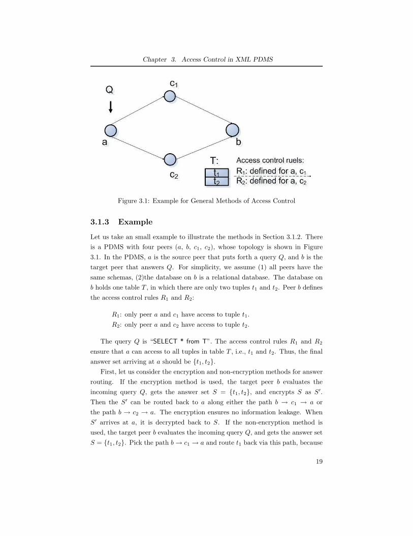
3.1.3 Example
Let us take an small example to illustrate the methods in Section 3.1.2. There
is a PDMS with four peers (a, b, c1, c2), whose topology is shown in Figure
3.1. In the PDMS, a is the source peer that puts forth a query Q, and b is the
target peer that answers Q. For simplicity, we assume (1) all peers have the
same schemas, (2)the database on b is a relational database. The database on
b holds one table T , in which there are only two tuples t1 and t2. Peer b defines
the access control rules R1 and R2:
R1: only peer a and c1 have access to tuple t1.
R2: only peer a and c2 have access to tuple t2.
The query Q is “SELECT * from T”. The access control rules R1 and R2
ensure that a can access to all tuples in table T , i.e., t1 and t2. Thus, the final
answer set arriving at a should be {t1, t2}.
First, let us consider the encryption and non-encryption methods for answer
routing. If the encryption method is used, the target peer b evaluates the
incoming query Q, gets the answer set S = {t1, t2}, and encrypts S as S′.
Then the S′ can be routed back to a along either the path b → c1 → a or
the path b → c2 → a. The encryption ensures no information leakage. When
S′ arrives at a, it is decrypted back to S. If the non-encryption method is
used, the target peer b evaluates the incoming query Q, and gets the answer set
S = {t1, t2}. Pick the path b→ c1 → a and route t1 back via this path, because
19
Chapter 3. Access Control in XML PDMS
peer c1 just has access to t1 (according to R1) but no access to t2. Similarly,
pick the path b→ c2 → a and route t2 back via this path, because peer c2 just
has access to t2 (according to R2) but no access to t1.
Secondly, let us consider the evaluating and rewriting methods. Suppose we
use the non-encryption answer routing method and route the computed answer
backtracking the query incoming path. Consider the path a → c1 → b. If the
evaluating method is used, the query Q is routed along a→ c1 → b as initially
rewritten, keeping an annotation of all passing peers {a, c1}. When Q arrives
at b, b notices the annotation {a, c1} and uses the relevant access control rules
R1 and R2 to rewrite Q into Q′. The answer is evaluated from Q′ and routed
back along b → c1 → a. If the rewriting method is used, we must make sure
that R1 has been distributed to a and c1, and R2 has been distributed to a and
c2. Consider the path a → c1 → b. The query Q is first rewritten into Q′ at a
according to rules R1 and R2, which ensures the answer of Q′ can be accessed
by a. Next, when Q′ arrives at c1, it is rewritten into Q′′ according to R1, which
ensures the answer of Q′′ can be accessed by c1. Thus Q′′, which will finally
arrive at b, ensures its answer can be accessed by both a and c1. After Q′′ is
computed at b, the answer can be safely routed back to a via b→ c1 → a.
3.2 Access Control Policy (ACP) Formal
Definition
Having a general idea about the access control problems in a PDMS, we will
take the first step into our own solution.
As shown in Chapter 2, access control policy (ACP) is a flexible, expressive
and fine-grained approach. Once specified, ACPs are platform-independent and
can be easily transformed and distributed in a PDMS environment. Thus our
work adopts ACP as the access control model for peer databases. Our whole
access control scheme is based on such an ACP model.
Let us propose the ACP formal definition and syntax for the XML PDMS:
Definition 3.1 (Access Control Policy (ACP)) An access control policy ACP
is defined in the following form: +/ − R(u, x) ← SLA(target, u), q(x). Such a
policy defines that a set of peers u has read access to some target data elements
x under the restrictions of service level agreement SLA(target, u) and object
constraint q(x).
20
Chapter 3. Access Control in XML PDMS
• +/- denotes authorize/deny access.
• R denotes that it is a READ ACP. That means, the authorized peers will
have the READ privilege of the target data elements.
• u denotes the set of subject/user/role, which are the identifiers of users in
the system and often refer to peers.
• x denotes the set of target data elements. Here we define target schema
as the data schema on which the ACP has effect. Target data elements
are some elements in the data schema, which are those elements that the
ACP is allowing or denying access to.
• target refers to the target peer, who is the owner of the target schema.
• SLA(target, u) denotes a predicate that tests the role of the peers, i.e.
whether peers u have a service level agreement with the target peer. If u
satisfies SLA(target, u), u will have the access privilege defined by this
ACP.
• q(x) is the DB predicate or value constraints, which expresses the con-
straints on the target XML document. q(x) can be a conjunction of atoms.
An atom can be a variable binding, a relational expression of equality or
inequality. However, the expression of q(x) doesn’t mean these constraints
only have the domain of the target elements x, normally they are the con-
straints on all related elements. In this abstract expression, we don’t treat
x as the domain of q(x).
• The authorize/deny access on an element x is automatically propagated
to its subelements. We believe it makes sense to be consistent with the
semantics of XQuery answers.
• Similarly, we use W (u, x) to denote a WRITE/EDIT ACP. That means,
the authorized peers will have the WRITE privilege of the target data ele-
ments.
Without any specification, the strength of SLA(target, u) in an ACP may
become boundless. We place a limit on what SLA(target, u) can contribute:
SLA(target, u) only checks the agreement relationship between peers, i.e. which
peers are authorized the privilege on target database by this ACP. In some
cases, an ACP needs to match the peer’s ID with an element value in the target
21
Chapter 3. Access Control in XML PDMS
database. For example, assume there is an element in the database of my peer
about the visitor’s ID. My peer defines an ACP that only the classmate peers
have access to my database information. The ACP needs a way to compare the
visitor peer’s ID with the element value in my database. In our ACP syntax,
we use a function compatible(x, y) to deal with the match of a peer ID and an
element value in the target database. The basic ACP structure and use of the
SLA(target, u) and compatible(x, y) functions are illustrated in the examples
of next section.
3.3 PDMS Scenarios with ACP Examples
In the previous section, we introduced the formal syntax of an ACP. In this
section we illustrate it with some concrete PDMS scenarios and ACP instances.
The examples show that the ACP syntax is XPath-based and XQuery-compatible.
It makes a good basis for our later XML query rewriting algorithm.
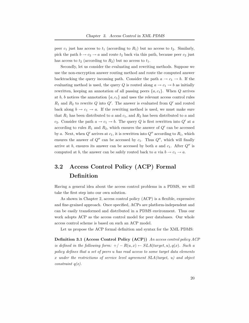
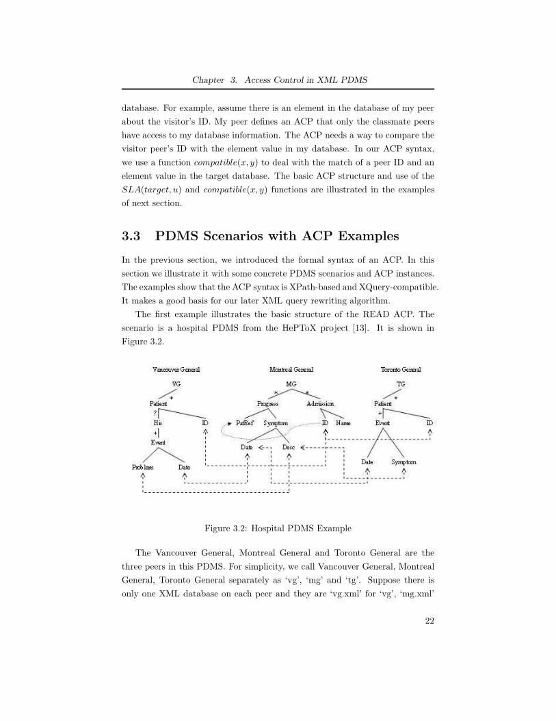
The first example illustrates the basic structure of the READ ACP. The
scenario is a hospital PDMS from the HePToX project [13]. It is shown in
Figure 3.2.
Figure 3.2: Hospital PDMS Example
The Vancouver General, Montreal General and Toronto General are the
three peers in this PDMS. For simplicity, we call Vancouver General, Montreal
General, Toronto General separately as ‘vg’, ‘mg’ and ‘tg’. Suppose there is
only one XML database on each peer and they are ‘vg.xml’ for ‘vg’, ‘mg.xml’
22
Chapter 3. Access Control in XML PDMS
for ‘mg’, ‘tg.xml’ for ‘tg’.
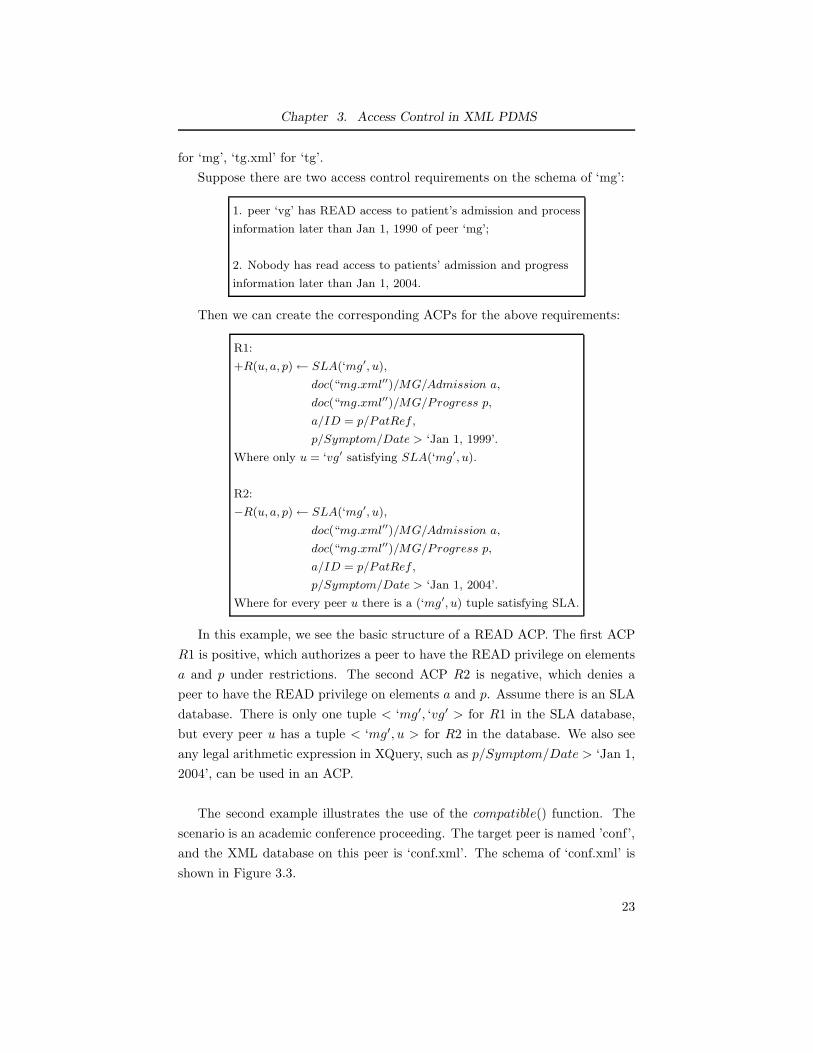
Suppose there are two access control requirements on the schema of ‘mg’:
1. peer ‘vg’ has READ access to patient’s admission and process
information later than Jan 1, 1990 of peer ‘mg’;
2. Nobody has read access to patients’ admission and progress
information later than Jan 1, 2004.
Then we can create the corresponding ACPs for the above requirements:
R1:
+R(u, a, p)← SLA(‘mg′, u),
doc(“mg.xml′′)/MG/Admission a,
doc(“mg.xml′′)/MG/Progress p,
a/ID = p/PatRef ,
p/Symptom/Date > ‘Jan 1, 1999’.
Where only u = ‘vg′ satisfying SLA(‘mg′, u).
R2:
−R(u, a, p)← SLA(‘mg′, u),
doc(“mg.xml′′)/MG/Admission a,
doc(“mg.xml′′)/MG/Progress p,
a/ID = p/PatRef ,
p/Symptom/Date > ‘Jan 1, 2004’.
Where for every peer u there is a (‘mg′, u) tuple satisfying SLA.
In this example, we see the basic structure of a READ ACP. The first ACP
R1 is positive, which authorizes a peer to have the READ privilege on elements
a and p under restrictions. The second ACP R2 is negative, which denies a
peer to have the READ privilege on elements a and p. Assume there is an SLA
database. There is only one tuple < ‘mg′, ‘vg′ > for R1 in the SLA database,
but every peer u has a tuple < ‘mg′, u > for R2 in the database. We also see
any legal arithmetic expression in XQuery, such as p/Symptom/Date > ‘Jan 1,
2004’, can be used in an ACP.
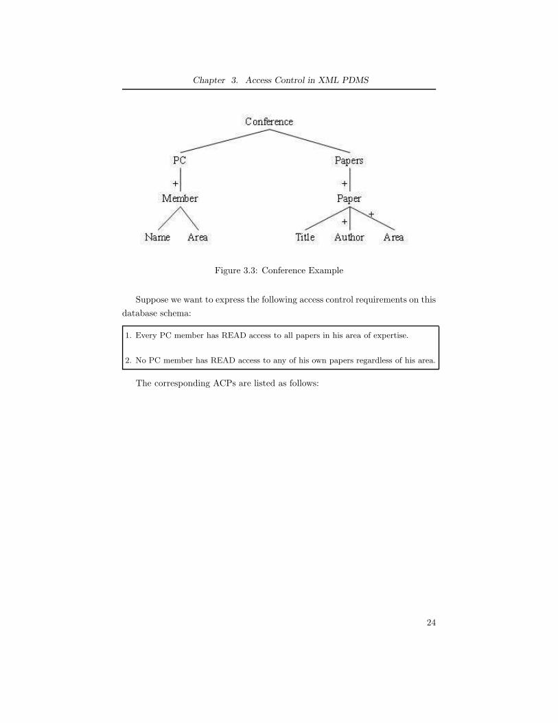
The second example illustrates the use of the compatible() function. The
scenario is an academic conference proceeding. The target peer is named ’conf’,
and the XML database on this peer is ‘conf.xml’. The schema of ‘conf.xml’ is
shown in Figure 3.3.
23
Chapter 3. Access Control in XML PDMS
Figure 3.3: Conference Example
Suppose we want to express the following access control requirements on this
database schema:
1. Every PC member has READ access to all papers in his area of expertise.
2. No PC member has READ access to any of his own papers regardless of his area.
The corresponding ACPs are listed as follows:
24
Chapter 3. Access Control in XML PDMS
R1:
+R(u, p)← SLA(′conf ′, u),
doc(“conf.xml′′)/PC/Member pm,
doc(“conf.xml′′)/Papers/paper p,
compatible(u, pm/Name),
pm/Area = p/Area.
Where SLA(‘conf ′, u) defines the membership relation of any user
for the conference, the function compatible() checks matching of
a peer ID u and a PC member’s name.
R2:
−R(u, p)← SLA(′conf ′, u),
doc(“conf.xml′′)/PC/Member pm,
doc(“conf.xml′′)/Papers/paper p,
p/Author pa,
pa = pm/Name,
compatible(u, pm/Name).
Where SLA(‘conf ′, u) defines the membership relation of any user for
the conference, compatible() checks matching of a peer ID u and a
PC member’s name.
In this example, we see the use of the function compatible(). As described
in Section 3.2, the function compatible() checks to see if a peer ID matches an
element in the target database.
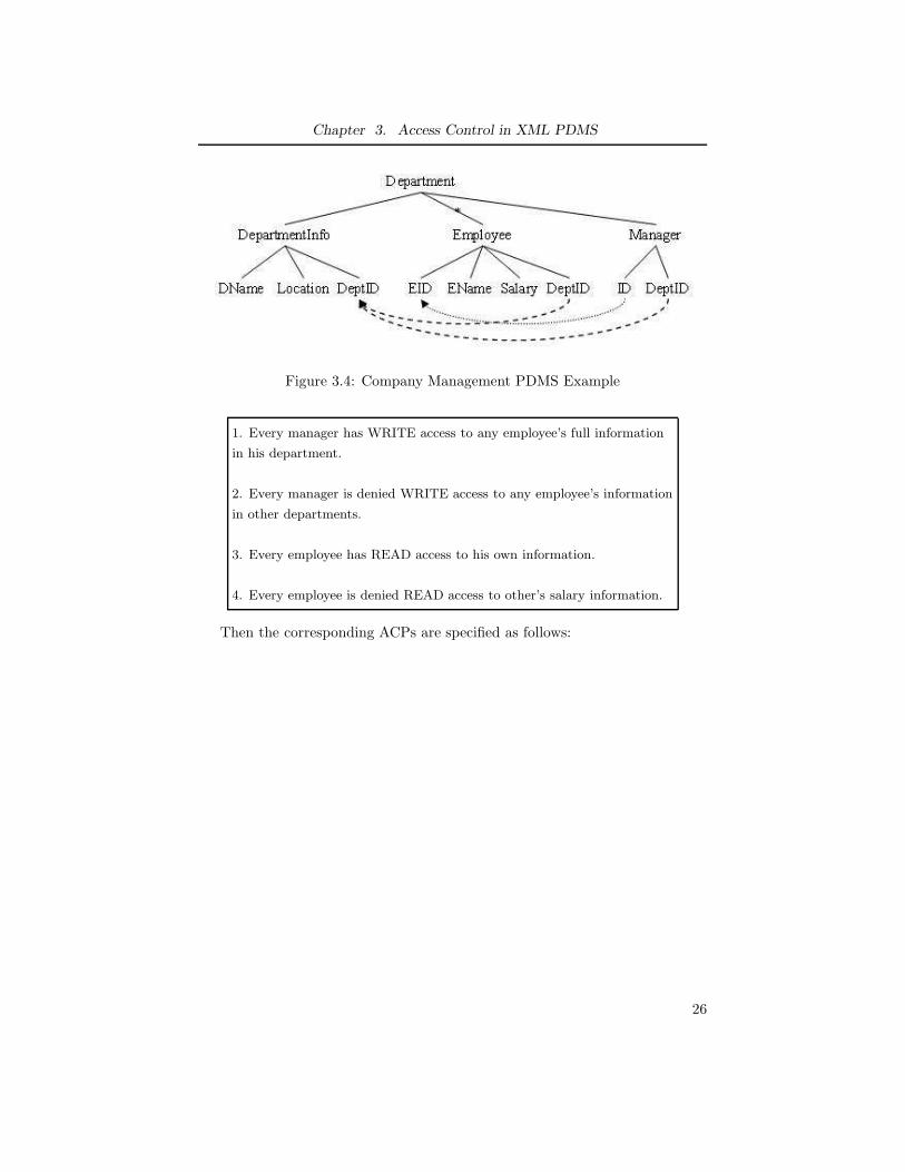
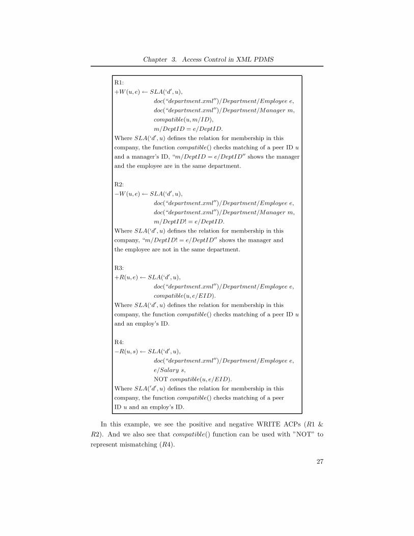
The third example illustrates the WRITE ACP and the negative use of the
compatible() function. The scenario is a company management PDMS. This
company has several departments. Each department server is a autonomous
peer. Each department has a manager and some employees. (The manager is
also an employee.) The database schema for one department peer is shown in
Figure 3.4:
We name the peer in the figure as ‘d’, its XML database as ‘department.xml’.
Suppose we need to express the following access control requirements on the
schema of ‘d’:
25
Chapter 3. Access Control in XML PDMS
Figure 3.4: Company Management PDMS Example
1. Every manager has WRITE access to any employee’s full information
in his department.
2. Every manager is denied WRITE access to any employee’s information
in other departments.
3. Every employee has READ access to his own information.
4. Every employee is denied READ access to other’s salary information.
Then the corresponding ACPs are specified as follows:
26
Chapter 3. Access Control in XML PDMS
R1:
+W (u, e)← SLA(‘d′, u),
doc(“department.xml′′)/Department/Employee e,
doc(“department.xml′′)/Department/Manager m,
compatible(u,m/ID),
m/DeptID = e/DeptID.
Where SLA(‘d′, u) defines the relation for membership in this
company, the function compatible() checks matching of a peer ID u
and a manager’s ID, “m/DeptID = e/DeptID′′ shows the manager
and the employee are in the same department.
R2:
−W (u, e)← SLA(‘d′, u),
doc(“department.xml′′)/Department/Employee e,
doc(“department.xml′′)/Department/Manager m,
m/DeptID! = e/DeptID.
Where SLA(‘d′, u) defines the relation for membership in this
company, “m/DeptID! = e/DeptID′′ shows the manager and
the employee are not in the same department.
R3:
+R(u, e)← SLA(‘d′, u),
doc(“department.xml′′)/Department/Employee e,
compatible(u, e/EID).
Where SLA(‘d′, u) defines the relation for membership in this
company, the function compatible() checks matching of a peer ID u
and an employ’s ID.
R4:
−R(u, s)← SLA(‘d′, u),
doc(“department.xml′′)/Department/Employee e,
e/Salary s,
NOT compatible(u, e/EID).
Where SLA(′d′, u) defines the relation for membership in this
company, the function compatible() checks matching of a peer
ID u and an employ’s ID.
In this example, we see the positive and negative WRITE ACPs (R1 &
R2). And we also see that compatible() function can be used with ”NOT” to
represent mismatching (R4).
27
Chapter 3. Access Control in XML PDMS
3.4 Semantics of PDMS Query-Answering
under ACPs
Given that all ACPs are specified and distributed as needed, what is the answer
semantics of the PDMS query-answering? More specifically, what kind of answer
do we expect to get after a query is put forth at a peer in a PDMS? In this
section, we will formalize the semantics of PDMS query answering under ACPs.
The access control issue is orthogonal to the issue of schema heterogeneity.
Thus, to simplify the problem, we assume that all peers use the same schema.
This allows us to tackle access control without adding in the complications of
schema heterogeneity. We leave the addition of schema heterogeneity to the
problem as future work. Besides, we do not distinguish a peer with a requester.
Several requesters may put queries on a peer to the whole PDMS. We assume
all queries are put forth by a same peer. This simplification will help us to see
the nature of the semantics problem.
Firstly let us start with the answer semantics of a PDMS without access
control. Given a PDMS with n peers (p1, p2,..., pn), each peer has a local
database DBpi (i = 1..n). In a practical PDMS, there may be some peers who
are virtual nodes and do not have a local database. However, this case is not
considered here. Suppose a query Q is put on p1. The full answer set returned
at p1 is the union of the answer set from every peer. For each peer pi(i = 1..n),
the partial answer set is Q(DBpi) (i = 1..n). Thus, the semantics of answer
returned by the PDMS is⋃
i Q(DBpi) (i = 1..n).
Next let us add the factor of access control. Let AVp1(DBpi
) be the access
view for peer p1 on peer pi’s database, which holds for a centralized system
using any access control policy model. For each peer pi (i = 1..n), the answer
that p1 has the permission to see on DBpiis Q(AVp1
(DBpi)). Thus, naively,
one might expect the full answer returned to p1 to be⋃
i Q(AVp1(DBpi
)), where
i = 1..n. But it is not correct. Because any answer tuple needs to be routed
from the answering peer pi to p1 via some other peers. It must ensure that an
answer tuple can be accessed by every peer along the routing path. Consider
this problem in another way: when a query is transmitted from p1 to pi, the
query will pass via some other peers, and these peers will add access control
constraints on the access view of pi to make the final answer set smaller than
Q(AVp1(DBpi
)).
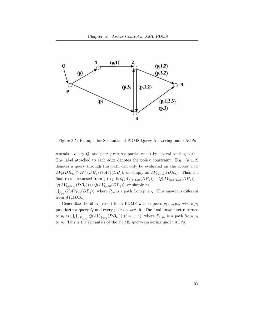
Consider the following example. Figure 3.5 is a PDMS topology. Suppose
28
Chapter 3. Access Control in XML PDMS
Figure 3.5: Example for Semantics of PDMS Query Answering under ACPs
p sends a query Q, and peer q returns partial result by several routing paths.
The label attached to each edge denotes the policy constraint. E.g. (p, 1, 2)
denotes a query through this path can only be evaluated on the access view
AVp(DBq) ∩ AV1(DBq) ∩ AV2(DBq), or simply as AV(p,1,2)(DBq). Thus the
final result returned from q to p is Q(AV(p,1,2)(DBq)) ∪Q(AV(p,1,2,3)(DBq)) ∪
Q(AV(p,3,2)(DBq)) ∪Q(AV(p,3)(DBq)), or simply as⋃
PpqQ(AVPpq
(DBq)), where Ppq is a path from p to q. This answer is different
from AVp(DBq).
Generalize the above result for a PDMS with n peers p1, ..., pn, where p1
puts forth a query Q and every peer answers it. The final answer set returned
to p1 is⋃
i
⋃Pp1pi
Q(AVPp1pi(DBpi
)) (i = 1..n), where Pp1piis a path from p1
to pi. This is the semantics of the PDMS query-answering under ACPs.
29
Chapter 4
Strategies and Options for
the Query-Answering
Process
Chapter 3 presented the syntax of the access control policy and showed that it is
expressive enough to specify fine-grained access control on peers’ local database.
But we have not described how to enforce ACPs, or say, how ACPs are used in
the PDMS query answering process.
Intuitively, a query-answering process can be clearly divided into two parts:
query transmitting and answer routing. Thus we separate a query-answering al-
gorithm into two parts: a (query transmitting) strategy and an (answer routing)
option.
Study on the general methods for access control (Section 3.1.2) inspires our
designing strategies and options. In this chapter, we present the intuition (Sec-
tion 4.1) and formal definitions of a strategy and an option (Section 4.2), then
describe the basic assumptions (Section 4.3) and our designed strategies and
options that make use of access control polices (Section 4.4).
4.1 Intuition
The security problem arising in a PDMS concentrates on the query-answering
process. Such a query-answering process is under the control of a distributed,
runtime algorithm. The algorithm distributes the query or its rewritten form
from the source peer to many target peers and retrieves answers from these
target peers to the source peer. The example used in Section 3.1.3 is helpful for
illustrating the problem. Please refer to Figure 3.1. The example setting is ex-
actly the same, including the topology, peers, ACPs, query, and so on. Assume
a non-encryption query-answering algorithm controls the query-answering pro-
30
Chapter 4. Strategies and Options for the Query-Answering Process
cess of the PDMS. When a query Q is put forth at peer a, the query-answering
algorithm transmits Q via every path from peer a to peer b, and for each path
Q is rewritten to a new query according to relevant ACPs. Let the rewritten
query via path a → c1 → b be Q′, the rewritten query via path a→ c2 → b be
Q′′. Then the answer set for Q′ is {t1}, and the answer set for Q′′ is {t2}. If the
query-answering algorithm routes {t1} back to a via b → c2 → a, the informa-
tion leakage arises. Because peer c2 is not authorized to access t1 by any ACP.
Thus, to ensure no information leakage, the query-answering algorithm must
route {t1} back to a via b → c1 → a. Likely, the query-answering algorithm
must route {t2} back to a via b→ c2 → a.
To study the problem, we concentrate on the basic building block: trans-
mitting a query asked by a single source peer to a single target peer, and then
routing the answer set from that target peer back to the source peer. When a
query Q is posed at a source peer c, the answer set for Q from any target peer
containing relevant data needs to be computed and routed to c, modulo ACPs.
Thus, the overall problem is built up on basis of the simpler problem of single
source peer and single target peer.
The above pair-wise idea makes clear the building block of the query-answering
algorithm. Next, let us consider the query-answering process for a pair of given
source peer and target peer. The process can be clearly divided into two se-
quential, non-overlapping parts:
I. query transmitting: informally speaking, transmitting the rewritten
queries of the original query from the source peer to the target peer via
some paths;
II. answer routing: informally speaking, routing back the set of answer
tuples from the target peer to the source peer via some paths.
From now on, we call an algorithm handling Part I as Query Transmitting
Strategy, or Strategy ; and an algorithm handling Part II as Answer Routing
Option, or Option. Then a distributed query-answering algorithm is composed
of a Strategy and an Option. We will use a (Strategy, Option) pair to denote
a query-answering algorithm, simply as an (S, O) pair. The properties of an
(S, O) pair are those of the corresponding query-answering algorithm.
31
Chapter 4. Strategies and Options for the Query-Answering Process
4.2 Formal Definitions for Strategy and Option
In this section, we will present the formal definitions for a Strategy and an
Option. First of all, we define some terminology, which will be widely used in
later discussion:
• ACP of x for y: x’s definition of what y can have access to x’s data, where
x and y are both peers
• associated peer c of ACP A: peer c is defined in ACP A to access some
data of another peer
• V : a set of peers in a graph
• a: the source peer
• b: the target peer
• D: a database
• Db: the database residing on b
• Q: a query
• Q(D): the database to hold the answer of evaluating Q on D.
• t: an (answer) tuple in some Q(D). Here the word ”tuple” refers to the
building block of Q(D). For example, if D is a relational database and Q
is a SQL query, t is a tuple in the relation Q(D); if D is an XML database
and Q is an XQuery, t is an XML subtree or a combination of variable
values.
• pL(D): a new database, which defines part of database D that can be
accessed for all peers in the set L. If L contains just one peer c, pL(D)
can be simply written as pc(D) instead of p{c}(D).
• P : a path (sometimes it also refers to the set of all peers in a path if
there is no ambiguity). Note that throughout we assume that any path
conforms to the given topology.
• Pa→b: a path from a to b
• Pa→b: the set of all paths from a to b
32
Chapter 4. Strategies and Options for the Query-Answering Process
The formal definitions for Strategy and Option that are used to transmit
queries and answers over a single source peer and target peer set are shown in
Definition 4.1 and 4.2. As mentioned in the previous section, this is the building
block of the general case of one source peer and many target peers.
Definition 4.1 (Strategy) Given source peer a, target peer b, query Q, choose
a set of paths from a to b, and ∀ such path: transmit some rewritten query Q′
to b.
Definition 4.2 (Option) Given source peer a, target peer b, query Q, a set of
tuples S at b, choose a set of paths Pb→V from b to V , where V is a set of peers,
and send each tuple t ∈ S down 0 or more paths ∈ Pb→V .
These definitions are at an abstract level. Note that “choose a set of paths”
refers to the fact that the strategy or option will decide which paths the query
or tuples will be sent down and does not reply that the path will be chosen
apriori. The combination of a strategy and an option decides the distributed,
runtime features of the query-answering process in a PDMS. Because there is
little complication for query evaluation (i.e. generating answer tuples at the
target peer), it is regarded as a separate phase between a Strategy and an
Option, and not included in either of them.
4.3 Basic Assumptions
To evaluate the approach, we created a number of general strategies and options.
These strategies and options cover quite a broad spectrum, so we believe that
most other strategies and options are variants of them. In this section, we
propose a few important assumptions, which build the basis for our strategies
and options.
1. Databases residing on all peers have the same schema. Although
this assumption is not true for a realistic PDMS, schema heterogeneity
will not affect the essence of security problem. Query rewriting or data
transformation among different schemas is orthogonal to access control.
This assumption simplifies the linguistic expressions, and allows us to
concentrate on security issues in the query-answering process. So in later
discussion, we ignore the query rewriting only with respect to schema het-
erogeneity. We leave the addition of schema heterogeneity to the problem
as future work.
33
Chapter 4. Strategies and Options for the Query-Answering Process
2. When a query Q is transmitted along a path P , P is noted for Q.
Assume there is a trivial way to record passing peer ID’s with the routed
query Q. It is handy and costs little. We ignore the cost of this task in
later discussion.
3. Peers don’t collude with each other. In other words, peers will not
viciously share information to seek unauthorized data. Given peers c1, c2,
c3, tuple t ∈ Dc1, and c2 has got t from c1, which is authorized by c1’s
ACPs. Then c2 can not share t with c3 unless c2 have enough knowledge
(annotations, ACPs) from c1 to verify c3’s right to access t. Else we call
it an illegal behavior. We don’t consider such illegal behaviors, even when
we discuss information leakage in Section 5.1.
4. Assume a tuple t can be accessed by peer c1 and has been routed
to c1. t can be distributed from peer c1 to another peer c2, only if
c1 has sufficient witness from t’s source peer s, on whose database
t is computed. That means, even c1 has the right to access t, it doesn’t
have the right to willfully distribute t. The concrete cases we are concerned
include: (1) c1 must respect t’s annotation. More specifically, if t has been
routed to c1 together with its annotation At (the set of safe peer ID’s),
c1 obeys t’s annotation only to share it with peers d ∈ At. (2) c1 must
have all ACPs of s for c2 to determine if c2 can access t. The precondition
for this assumption is: each peer behaves legally according to the query-
answering algorithm and trusts data from other peers. More specifically,
if peer c1 receives tuple t, c1 trusts any information about t received from
other peers.
5. Let A1 be an ACP of the target peer b for peer c1. If A1 is
required for rewriting a query Q at c1, A1 must have been dis-
tributed to c1 in a safe way. According to the definition, Strategy is
a runtime algorithm. Distributing ACPs to requiring peers is the prepa-
ration for a strategy. Although we don’t consider how to perform this
work in a strategy, it is indeed a precondition of a strategy. Later we
will elaborate on this task and count in its cost in the cost model and in
(Strategy, Option) pairs’ costs.
6. Let A1 be an ACP of the target peer b for peer c1. Assume c1
and c2 are adjacent peers in the P2P network, and c2 attempts to
route an answer tuple t to c1. If A1 is required at c2 to determine
34
Chapter 4. Strategies and Options for the Query-Answering Process
whether c1 has access to tuple t, A1 must have been distributed
to c2 in a safe way. One might think it is risky to distribute the ACP
A1 for peer c1 to peer c2, which will cause information leakage. But in
fact it is safe on condition of Assumption 3 and Assumption 4. Under
Assumption 3 and 4, even c2 knows ACP A1, there is no way for c2 to
get illegal data from c1. Because c1 will use ACPs of target peer b for
c2 to determine whether send b’s data to c2. According to the definition,
an option is a runtime algorithm. Distributing ACPs to requiring peers
is just the preparation for an option. We don’t consider how to conduct
it in an option. But later we will elaborate on this task and count in the
cost of it in our cost model and in (Strategy, Option) pairs’ costs.
Without special claim, Assumption 1 to 4 hold for any strategy and option.
Assumption 5 and 6 hold when the “if” conditions are met.
4.4 Strategies and Options Designed
In this section, we will present the strategies and options we designed. The
terminology for these strategies and options is listed at the beginning of Section
4.2. The basic assumptions are listed in Section 4.3.
The following are the strategies we worked out, which make use of ACPs.
We use S1 to S4 to denote them.
S1 Proactive Rewriting: Assumption 5 holds. ∀ path P ∈ Pa→b, S1 trans-
mits Q along P by: at each peer c ∈ P , when the query, thus far Q′, is
transmitted to it, it transmits Q′′ to the next peer in P , where Q′′ = Q′
rewritten to adhere to ACPs of b for c.
S2 Lazy Rewriting – Dumb: For one path P ∈ Pa→b, S2 transmits Q via
P . When Q is transmitted at b, Q is rewritten into Q′ = Q rewritten to
adhere to ACPs of b for all peers in the PDMS.
S3 Lazy Rewriting – Path: ∀ path P ∈ Pa→b, S3 transmits Q via P . When
Q is transmitted at b, Q is rewritten into Q′ = Q rewritten to adhere to
ACPs of b for all peers in P .
S4 Jobless: ∀ path P ∈ Pa→b, S4 just transmits Q via P .
35
Chapter 4. Strategies and Options for the Query-Answering Process
In order to make Si (i=1..4) work well, there are necessary obligations for
peers in the PDMS:
• For S1, ∀ peer c (except the target peer b): c use all ACPs of b for c to
correctly rewrite the received query Q′ into the new query Q′′ ∧ c route
Q′′ to the next peer.
• For S2 and S3, ∀ peer c (except the target peer b): c forwards the received
query Q to the next peer. For the target peer b: b correctly rewrites the
received query using required ACPs.
• For S4, ∀ peer c (except the target peer b): c forwards the received query
Q to the next peer.
The following are the options we designed, which make use of ACPs. We
use O1 to O6 to denote them.
O1 Whole – Backtracking: Given target peer b, database D at b, query Q
that has been transmitted at b via some path P ∈ Pa→b, Q and P have
been chosen by some strategy. Q(D) is regared at b as the answer set.
Annotate answer set Q(D) with path P . At each peer c ∈ P , c routes
Q(D) to the previous peer in P until c = a.
O2A Whole – Sub1: Given target peer b, database D at b, query Q that has
been transmitted at b via some path P ∈ Pa→b , Q and P have been
chosen by some strategy. pP (Q(D)) ⊆ Q(D) is regarded as the answer set
at b. Annotate answer set with path P . Choose a path P ′ s.t. P ′ ∈ Pb→a
∧ P ′ ⊆ P . Route pP (Q(D) down P ′.
O2B Whole – Sub2: Given target peer b, database D at b, query Q that has
been transmitted at b via some path P ∈ Pa→b , Q and P have been
chosen by some strategy. Q(D) is regarded as the returned answer set at
b. Annotate answer set with path P . Choose a path P ′ s.t. P ′ ∈ Pb→a ∧
P ′ ⊆ P . Route Q(D) down P ′.
O3 Whole – Target Annotating: Given target peer b, database D at b,
query Q that has been transmitted at b via some path P ∈ Pa→b , Q
and P have been chosen by some strategy. The returned answer set at
b is A = pP (Q(D)) ⊆ Q(D). Use ACPs of b to decide the safe peer list
36
Chapter 4. Strategies and Options for the Query-Answering Process
L = {c|pc(A) = A}. Annotate the answer set A with L. Choose a path
P ′ s.t. P ′ ∈ Pb→a ∧ P ′ ⊆ L. Route A× {L} down P ′.
O4A Whole – Dynamic Routing: Assumption 6 holds. Given target peer b,
database D at b, query Q that has been transmitted at b via some path
P ∈ Pa→b, Q and P have been chosen by some strategy. The returned
answer set at b is A = pP (Q(D)) ⊆ Q(D). ∀ peer c that received A: c
routes A to peer d if pd(A) = A, until A arrives at a.
O4B Whole – Dynamic Routing: Assumption 6 holds. Given target peer b,
database D at b, query Q that has been transmitted at b via some path
P ∈ Pa→b, Q and P have been chosen by some strategy. The returned
answer set at b is A = pP (Q(D)) ∪ S, where S is the set of supporting
elements. ∀ peer c that received A: c routes A to peer d if pd(A) = A,
until A arrives at a.
O5 Partition – Target: Given target peer b, database D at b, query Q at b,
Q has been chosen by some strategy. Q(D) is regarded as the answer set.
(1) Partition Q(D) as follows: let the partition K = K1, ..., Kn, where
n⋃
i=1
Ki = Q(D) ∧Ki ∩Kj = ∅(i 6= j)
∀Ki (i = 1..n), use ACPs of b to compute its annotation Li, where Li =
{c|pc(Ki) = Ki}
(2) ∀Ki(i = 1..n): if Ki ×{Li} arrives at peer c, c routes Ki ×{Li} to all
its neighbors d, where d ∈ Li.
O6A Dynamic Routing: Assumption 6 holds. Given target peer b, database
D at b, query Q at b, Q has been chosen by some strategy. The returned
answer set at b is Q(D). Let c be a peer who receives a subset K ⊆ Q(D).
∀c ∀ its neighbor d: c routes pd(K) to d. Notice: all parts sent by c to its
neighbors may not be disjointed.
O6B Dynamic Routing: Assumption 6 holds. Given target peer b, database
D at b, query Q at b, Q has been chosen by some strategy. The returned
answer set at b is A = Q(D)∪S, where S is the set of supporting elements.
Let c be a peer who receives a subset K ⊆ A. ∀c ∀ its neighbor d: c routes
pd(K) to d. Notice: all parts sent by c to its neighbors may not be
disjointed.
37
Chapter 4. Strategies and Options for the Query-Answering Process
In O4B and O6B, there is a new concept “supporting element”. Supporting
elements refer to the elements that should be projected out in the answer tuples
but are needed for later usage, especially as filters of ACPs to determine the
safe peers. In O4B and O6B, without help of tuple annotations, it is necessary
to keep supporting elements within the answer tuples during the answer routing
process.
In O5, the notation “Ki × {Li}” is mainly intended for logical correctness.
It doesn’t necessarily mean to attach each answer tuple t in Ki with Li. An
implementation for O5, which factors away the common repeating Li for all
the tuples in a set Ki, is entirely consistent with this notation. Likewise the
explanation works for “A× {L}” in O3.
In order to make Oi (i=1..6) work well, there are necessary obligations for
peers in the PDMS:
• For O1, ∀ peer c (except the source peer a) who receives/has an answer
set Q(D): c correctly routes Q(D) to the previous peer in path P . The
target peer b correctly annotates the answer set Q(D) with the path P .
• For O2A and O2B , ∀ peer c1 (except the source peer a) who receives/has
an answer set: c1 correctly routes the answer set to a peer c2 ∈ P . The
target peer b correctly annotates the answer set with the path P .
• For O3, ∀ peer c1 (except the source peer a) who receives/has an answer
set: c1 correctly routes the answer set to a peer c2 ∈ L. The target peer
b correctly annotates the answer set with the list L.
• For O4A and O4B , ∀ peer c1 (except the source peer a) who receives/has
an answer set: c1 uses all related ACPs to correctly find a safe peer c2 for
the answer set, and routes the answer set to c2.
• For O5, ∀ peer c1 (except the source peer a) who recieves/has a partition
Ki: c1 correctly routes Ki ∪ Li to a peer c2 ∈ Li. The target peer b cor-
rectly partitions Q(D) and annotates each partition Ki with an annotation
Li.
• For O6A and O6B , ∀ peer c (except the source peer a) who recieves/has a
partition K, ∀ peer d who is adjacent to peer c: c uses all related ACPs
to correctly compute and route pd(K) to peer d.
38

Chapter 4. Strategies and Options for the Query-Answering Process
The combination of any strategy and any option in this section forms a full
query-answering algorithm in a PDMS. In the next chapter, we will analyze the
information leakage and completeness properties of each (S, O) pair.
39
Chapter 5
Information Leakage and
Completeness for (S,O)
Pairs
The properties of a query-answering algorithm in a PDMS are those of an (S, O)
pair. Information leakage and completeness (of the answer) are among the most
important properties for an (S, O) pair.
In Section 5.1, we present the definition of information leakage (IL), the
sufficient and necessary condition for IL-free, then analyze the IL-free property
for all (S, O) pairs; in Section 5.2, we present the definition, the sufficient and
necessary condition for completeness, then analyze the completeness property
for all (S, O) pairs.
5.1 Information Leakage (IL)
The general sense of information leakage has been given in Section 3.1.1: some
protected data are accessed by unauthorized subjects. Information leakage for
a PDMS query-answering algorithm will be formally defined and studied in this
section.
5.1.1 Definitions
Avoiding information leakage is an important security issue in the PDMS query-
answering process. The information leakage we are concerned with concen-
trates on the query-answering process. Informally speaking, during the query-
answering process under control of an (S, O) pair, if peer c happens to receive
tuple t but isn’t authorized access to t, information leakage arises. Because
which peer to receive a tuple is determined by an (S, O) pair, we regard infor-
40
Chapter 5. Information Leakage and Completeness for (S,O) Pairs
mation leakage (or no information leakage) as a runtime property of an (S, O)
pair. Now let us make a formal definition for information leakage.
Definition 5.1 (Information Leakage (IL)) Given source peer a, target peer
b, database D at b, query Q, (S, O) has information leakage iff (i) ∃ path Pa→b
from a to b, Pa→b is chosen by S: S will send Q′ to b through Pa→b (S defines
the rewritten query Q′ from Q), (ii) ∃ a tuple t ∈ Q′(D), (iii) ∃ path Pb→x from
b to peer x, Pb→x is chosen by O: O will send t down that path ∧ ∃ c on that
path s.t. t /∈ pc(D). (S, O) is IL-free iff it has no information leakage, ∀ a, b,
Q.
IL-free is defined as the negation of Information Leakage in the above defi-
nition. For clarity, we reword the IL-free definition as follows:
Definition 5.2 (IL-Free) Given source peer a, target peer b, database D at
b, query Q, (S, O) has no information leakage iff (i) ∀ path Pa→b from a to b,
which is chosen by S: S will send Q′ to b through Pa→b (S defines the rewritten
query Q′ from Q), (ii) ∀ tuple t ∈ Q′(D), (iii) ∀ path Pb→x from b to peer x,
Pb→x is chosen by O: O will send t down that path ∧ ∀ c on that path s.t.
t ∈ pc(D). (S, O) is IL-Free iff it has no information leakage, ∀ a, b, Q.
The expression “t ∈ pc(D)” in the above definition needs to be explained. As
mentioned in Section 4.2, “pc(D)” denotes the part of database D that can be
accessed by peer c. Thus, “t ∈ pc(D)” means “tuple t is computed from D and
can be accessed by peer c”. From the viewpoint of schema, t and D have different
schemas and they are not comparable. Nevertheless, from the viewpoint of
information containment, t is contained in D. Since we are discussing IL-Free
in terms of information containment, we accept the expression “t ∈ pc(D)”.
Another similar expression is “Q(D) ⊆ D”. Given specific schemas of Q(D) and
D, there is no reason to say Q(D) ⊆ D. But from the viewpoint of information
containment, we accept “Q(D) ⊆ D” as a fact.
The above discussion is based on Assumption 3 & 4 of Section 4.3. We
don’t discuss the cases violating these assumptions. Furthermore, we assume no
caching here. As a common approach to accelerate the query-answering process,
caching is useful and worth noting. Nevertheless, as a supportive approach for
query-answering, caching is not in the central place. A system works smoothly
without caching. So at this moment we omit caching. We leave the security
problems involved in caching as future work.
41
Chapter 5. Information Leakage and Completeness for (S,O) Pairs
5.1.2 The Sufficient and Necessary Condition for IL-Free
IL-free is a security property for an (S, O) pair. However, we cannot expect to
use the IL-free definition to check if an (S, O) pair is IL-free. First, because
the IL-free definition is based on execution, you would need to run (S, O) on all
possible source peers, target peers, queries, query routing paths, etc. Secondly,
the IL-free definition has a tuple-based granularity, which is far different from
the description of a strategy or an option. So we need a general condition that
can be directly applied to the description of any (S, O) pair and check if it is
IL-free.
The following ideas are illuminating for finding such a condition:
• By the definitions of strategy and option, the answer tuples are computed
only at the target peer, and no more tuples are created in the answer
routing process. The option O determines whether to send an existing
tuple to a peer, but cannot create a new tuple and send it to a peer. Thus,
if peer c0 has an answer set T and option O will route the set T ′ from
peer c0 to its neighbor c, it must have T ′ ⊆ T .
• By the definition of IL-free, if the option O sends a tuple t to some peer c,
c must have access to t. In other words, O will send to c only the tuples
that c has access to.
Based on the above observation, we propose the sufficient & necessary
condition (SNC) for an arbitrary (S, O) pair to be IL-free.
SNC: For an (S, O) pair, ∀ source peer a, ∀ target peer b, ∀ query Q at a, ∀
peer c0, ∀ neighbors c of c0: c0 has answer set T and routes set T ′ ⊆ T to
c −→ T ′ ⊆ pc(T ).
Proof:
1. SNC is Sufficient. We shall show if (S, O) satisfies SNC, it also satisfies
the IL-free definition. Assume (S, O) satisfies SNC. Given source peer a, target
peer b, database D at b, query Q at a, rewritten query Q′ of Q at b, peer c0,
c0’s neighbor c, let the answer set at peer c0 be T and the set sent to peer c
be T ′ ⊆ T . By SNC, we know T ′ ⊆ pc(T ). Let an arbitrary tuple t ∈ T ′.
Since T ′ ⊆ pc(T ), it follows t ∈ pc(T ). By the definition of Strategy and
Option, we can infer T ⊆ Q′(D). Since we also have the fact Q′(D) ⊆ D in
sense of information containment, it follows T ⊆ D. Applying exactly the same
restriction pc() to both sides of this term, we get pc(T ) ⊆ pc(D). Since we
42
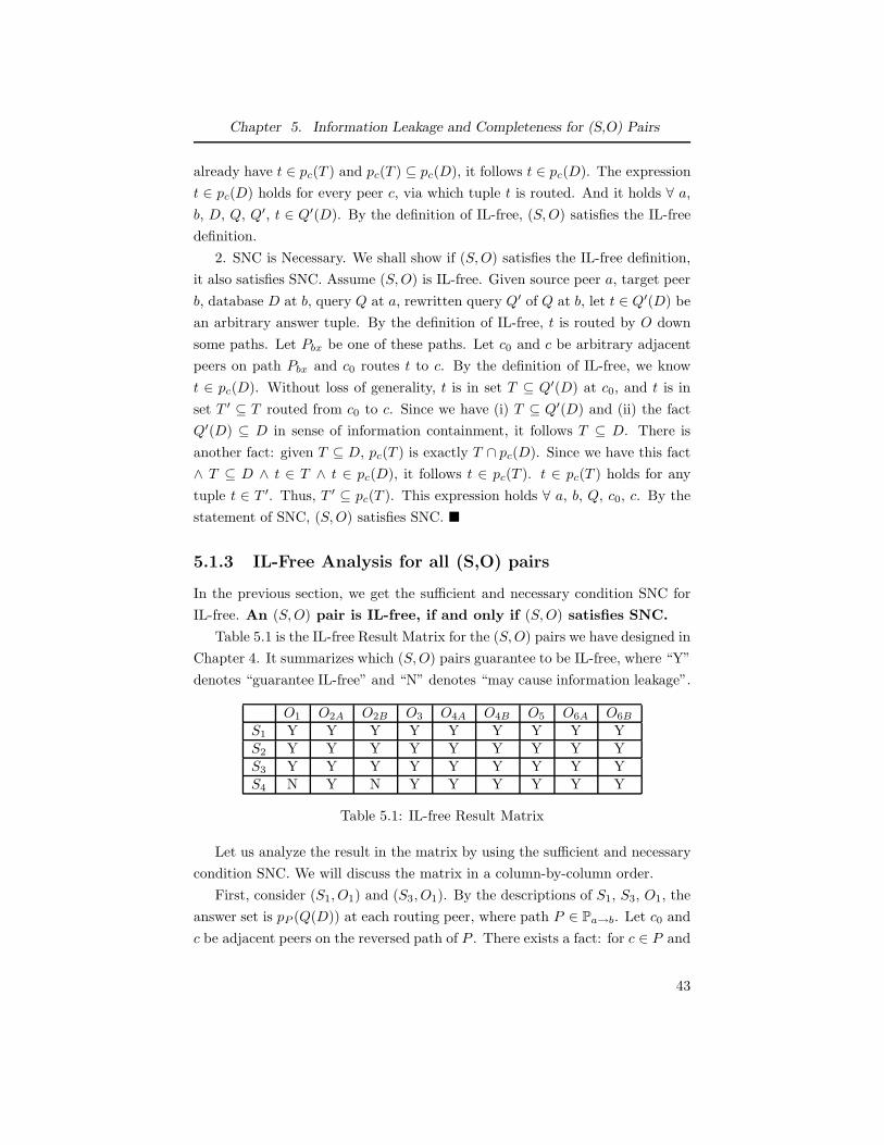
Chapter 5. Information Leakage and Completeness for (S,O) Pairs
already have t ∈ pc(T ) and pc(T ) ⊆ pc(D), it follows t ∈ pc(D). The expression
t ∈ pc(D) holds for every peer c, via which tuple t is routed. And it holds ∀ a,
b, D, Q, Q′, t ∈ Q′(D). By the definition of IL-free, (S, O) satisfies the IL-free
definition.
2. SNC is Necessary. We shall show if (S, O) satisfies the IL-free definition,
it also satisfies SNC. Assume (S, O) is IL-free. Given source peer a, target peer
b, database D at b, query Q at a, rewritten query Q′ of Q at b, let t ∈ Q′(D) be
an arbitrary answer tuple. By the definition of IL-free, t is routed by O down
some paths. Let Pbx be one of these paths. Let c0 and c be arbitrary adjacent
peers on path Pbx and c0 routes t to c. By the definition of IL-free, we know
t ∈ pc(D). Without loss of generality, t is in set T ⊆ Q′(D) at c0, and t is in
set T ′ ⊆ T routed from c0 to c. Since we have (i) T ⊆ Q′(D) and (ii) the fact
Q′(D) ⊆ D in sense of information containment, it follows T ⊆ D. There is
another fact: given T ⊆ D, pc(T ) is exactly T ∩ pc(D). Since we have this fact
∧ T ⊆ D ∧ t ∈ T ∧ t ∈ pc(D), it follows t ∈ pc(T ). t ∈ pc(T ) holds for any
tuple t ∈ T ′. Thus, T ′ ⊆ pc(T ). This expression holds ∀ a, b, Q, c0, c. By the
statement of SNC, (S, O) satisfies SNC. �
5.1.3 IL-Free Analysis for all (S,O) pairs
In the previous section, we get the sufficient and necessary condition SNC for
IL-free. An (S, O) pair is IL-free, if and only if (S, O) satisfies SNC.
Table 5.1 is the IL-free Result Matrix for the (S, O) pairs we have designed in
Chapter 4. It summarizes which (S, O) pairs guarantee to be IL-free, where “Y”
denotes “guarantee IL-free” and “N” denotes “may cause information leakage”.
O1 O2A O2B O3 O4A O4B O5 O6A O6B
S1 Y Y Y Y Y Y Y Y YS2 Y Y Y Y Y Y Y Y YS3 Y Y Y Y Y Y Y Y YS4 N Y N Y Y Y Y Y Y
Table 5.1: IL-free Result Matrix
Let us analyze the result in the matrix by using the sufficient and necessary
condition SNC. We will discuss the matrix in a column-by-column order.
First, consider (S1, O1) and (S3, O1). By the descriptions of S1, S3, O1, the
answer set is pP (Q(D)) at each routing peer, where path P ∈ Pa→b. Let c0 and
c be adjacent peers on the reversed path of P . There exists a fact: for c ∈ P and
43
Chapter 5. Information Leakage and Completeness for (S,O) Pairs
tuple set X , pP (X) = pc(pP (X)). Replacing X by Q(D) in the previous term,
we get pP (Q(D)) = pc(pP (Q(D))). Therefore, pP (Q(D)) ⊆ pc(pP (Q(D))).
Since (i) pP (Q(D)) ⊆ pc(pP (Q(D))) and (ii) by O1, peer c0 has answer set
pP (Q(D)) and routes exactly pP (Q(D)) to c, we see that (S1, O1) and (S3, O1)
satisfy SNC.
Let us consider (S2, O1). By S2 and O1, the answer set is pA(Q(D)) at
each routing peer, where A is the set of all peers in the P2P system. Let a
path P ∈ Pa→b, c0 and c be adjacent peers on the reversed path of P . There
exists a fact: for c ∈ P and tuple set X , pA(X) = pc(pA(X)). Replacing X by
Q(D) in this term, we get pA(Q(D)) = pc(pA(Q(D))). Therefore, pA(Q(D)) ⊆
pc(pA(Q(D))). Since (i) pA(Q(D)) ⊆ pc(pA(Q(D))) and (ii) by O1, peer c0 has
answer set pA(Q(D)) and routes exactly pA(Q(D)) to c, we see that (S2, O1)
satisfies SNC.
Let us consider (S4, O1). By S4 and O1, the answer set is Q(D) at each
routing peer. Let a path P ∈ Pa→b, c0 and c be adjacent peers on the reversed
path of P . By O1, c0 has the answer set Q(D) and routes exactly Q(D) to
c. However, there is no guarantee Q(D) ⊆ pc(Q(D)). That is to say, (S4, O1)
doesn’t satisfy SNC.
Let us consider (Si, O2A) (i = 1, 3, 4). By Si (i = 1, 3, 4) and O2A, the
answer set is pP (Q(D)) at each routing peer, where path P ∈ Pa→b. Let c0 and
c be adjacent peers on the returning path P ′. By O2A, we know P ′ ⊆ P . Thus,
c ∈ P . There exists a fact: for c ∈ P and tuple set X , pP (X) = pc(pP (X)).
Since we already have c ∈ P , replace X by Q(D) in the previous term, then get
pP (Q(D)) = pc(pP (Q(D))). Therefore, pP (Q(D)) ⊆ pc(pP (Q(D))). Since (i)
pP (Q(D)) ⊆ pc(pP (Q(D))) and (ii) by O2A, peer c0 has answer set pP (Q(D))
and routes exactly pP (Q(D)) to c, we see that (S1, O2A) (i = 1, 3, 4) satisfies
SNC.
Let us consider (S2, O2A). By S2 and O2A, the answer set is pA(Q(D))
at each routing peer, where A is the set of all peers in the P2P system. Let
c0 and c be adjacent peers on a returning path P ′. Since A is the set of all
peers in the P2P system, it follows c ∈ A. There exists a fact: for c ∈ A
and tuple set X , pA(X) = pc(pA(X)). Replacing X by Q(D) in this term, we
get pA(Q(D)) = pc(pA(Q(D))). Therefore, pA(Q(D)) ⊆ pc(pA(Q(D))). Since
(i) pA(Q(D)) ⊆ pc(pA(Q(D))) and (ii) by S2 and O2A, peer c0 has answer set
pA(Q(D)) and routes exactly pA(Q(D)) to c, we see that (S2, O2A) satisfies
SNC.
Let us consider (Si, O2B) (i = 1, 3). Analyzing the case exactly as (Si, O2A)
44
Chapter 5. Information Leakage and Completeness for (S,O) Pairs
(i = 1, 3, 4), we will get that (Si, O2B) (i = 1, 3) satisfies SNC.
Let us consider (S2, O2B). Analyzing the case exactly as (S2, O2A), we will
get that (S2, O2B) satisfies SNC.
Let us consider (S4, O2B). By S4 and O2B, the answer set is Q(D) at each
routing peer. Let c0 and c be adjacent peers on a returning path P ′. By O2B ,
c0 has the answer set Q(D) and routes exactly Q(D) to c. However, there is no
guarantee Q(D) ⊆ pc(Q(D)). Thus, (S4, O2B) doesn’t satisfy SNC.
Let us consider (Si, O3) (i = 1, 3, 4). By Si (i = 1, 3, 4) and O3, the an-
swer set is pP (Q(D)) at each routing peer, where path P ∈ Pa→b. Let c0
and c be adjacent peers on the returning path P ′. By O3, we know P ′ ⊆ L
and L = {c|pc(pP (Q(D))) = pP (Q(D))}. Since c ∈ P ′ ∧ P ′ ⊆ L ∧ L =
{c|pc(pP (Q(D))) = pP (Q(D))}, it follows pc(pP (Q(D))) = pP (Q(D)). There-
fore, pP (Q(D)) ⊆ pc(pP (Q(D))). Since (i) pP (Q(D)) ⊆ pc(pP (Q(D))) and (ii)
by O3, peer c0 has answer set pP (Q(D)) and routes exactly pP (Q(D)) to c, we
see that (S1, O3) (i = 1, 3, 4) satisfies SNC.
Let us consider (S2, O3). The analysis is almost the same as (Si, O3) (i =
1, 3, 4). The only difference is: the answer set is pA(Q(D)) at each routing peer,
where A is the set of all peers in the P2P system. We will get that (S2, O3)
satisfies SNC.
Let us consider (Si, O4A) (i = 1..4) and (Si, O4B) (i = 1..4). By O4A or O4B ,
the answer set is always some A at each routing peer. Let c0 and c be adjacent
peers on a returning path. By O4A or O4B , we know pc(A) = A. Therefore,
A ⊆ pc(A). Since (i) A ⊆ pc(A), (ii) by O4A or O4B, peer c0 has answer set
A and routes exactly A to c, we see that (Si, O4A) (i = 1..4) and (Si, O4B)
(i = 1..4) satisfy SNC.
Let us consider (Si, O5) (i = 1..4). By O5, the answer set is divided into
several partitions Ki (i = 1..n). Let Li be Ki’s annotation, c0 and c be adjacent
peers on a path to route Ki back. Since by O5 we know that Li = {c|pc(Ki) =
Ki} ∧ peer c ∈ Li, it follows pc(Ki) = Ki. Then Ki ⊆ pc(Ki). Since (i)
Ki ⊆ pc(Ki), (ii) by O5, peer c0 has answer set Ki and routes exactly Ki to c,
we see that (Si, O5) (i = 1..4) satisfies SNC.
Last, let us consider (Si, O6A) (i = 1..4) and (Si, O6B) (i = 1..4). Let c0
and c be adjacent peers on a returning path, K be the answer set that c0 has,
K ′ be the set that c0 routes to c. By O6A or O6B, we know K ′ = pc(K). Then
K ′ ⊆ pc(K). Thus, (Si, O6A) (i = 1..4) and (Si, O6B) (i = 1..4) satisfy SNC.
45
Chapter 5. Information Leakage and Completeness for (S,O) Pairs
5.2 Completeness
The general sense of completeness has been given in Section 3.1.1. It will be
formally defined and studied in this section.
5.2.1 Definitions
Given the source peer a, target peer b, and query Q at a, the answer set A
arriving at peer a may be different for different (S, O) pairs. The set A is
expected to be maximized, or Complete. Because the returned answer set A is
largely decided by the query-answering algorithm, the completeness is expected
to be a property of an (S, O) pair.
To define completeness, we need to make the following assumptions:
• As the property of an (S, O) pair, completeness is independent of
the query Q at source peer a. In other words, the completeness of the
answer set is not query-sensitive. If an (S, O) pair has the completeness
property, it ensures the completeness of the returned answer set for every
query Q.
• As the property of an (S, O) pair, completeness is independent
of the source peer a, the target peer b, and the database D at
b. Whatever a, b or D is, the completeness means that the corresponding
maximum answer set A should be retrieved from b to a. The completeness
of the answer set is independent of the source peer and target peer, given
an (S, O) pair.
Firstly, let us define the Ideal Completeness:
Definition 5.3 (Completeness I (Ideal Completeness)) Given source peer
a, target peer b, database D at b, query Q at a, (S, O) is complete for (a, b, Q)
iff: ∀ tuple t ∈ pa(Q(D)), ∃ path P from a to b ∧ ∃ path P ′ from b to a, S
sends Q′ to b ∧ t ∈ Q′(D) ∧ O sends t to a via P ′ ∧ t ∈ pc(D), ∀ peer c on P ′.
(S, O) is complete iff it is complete for (a, b, Q), ∀ a, b, Q.
The Ideal Completeness definition implies “maximal completeness based on
soundness”. In other words, it is the completeness on the condition of no infor-
mation leakage. Because the condition “t ∈ pc(D), ∀ peer c on P ′” in the above
definition ensures no information leakage. However, the Ideal Completeness
depends on the network topology and the target peer’s ACPs for other peers.
46
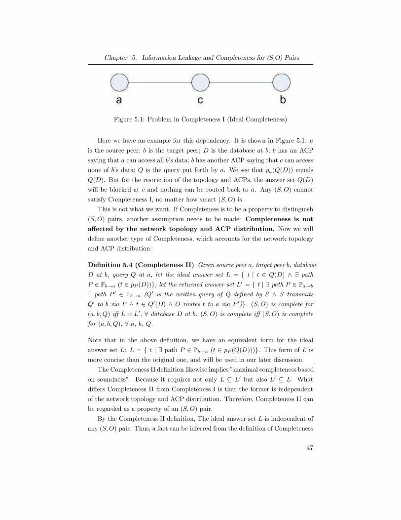
Chapter 5. Information Leakage and Completeness for (S,O) Pairs
Figure 5.1: Problem in Completeness I (Ideal Completeness)
Here we have an example for this dependency. It is shown in Figure 5.1: a
is the source peer; b is the target peer; D is the database at b; b has an ACP
saying that a can access all b’s data; b has another ACP saying that c can access
none of b’s data; Q is the query put forth by a. We see that pa(Q(D)) equals
Q(D). But for the restriction of the topology and ACPs, the answer set Q(D)
will be blocked at c and nothing can be routed back to a. Any (S, O) cannot
satisfy Completeness I, no matter how smart (S, O) is.
This is not what we want. If Completeness is to be a property to distinguish
(S, O) pairs, another assumption needs to be made: Completeness is not
affected by the network topology and ACP distribution. Now we will
define another type of Completeness, which accounts for the network topology
and ACP distribution:
Definition 5.4 (Completeness II) Given source peer a, target peer b, database
D at b, query Q at a, let the ideal answer set L = { t | t ∈ Q(D) ∧ ∃ path
P ∈ Pb→a (t ∈ pP (D))}; let the returned answer set L′ = { t | ∃ path P ∈ Pa→b
∃ path P ′ ∈ Pb→a (Q′ is the written query of Q defined by S ∧ S transmits
Q′ to b via P ∧ t ∈ Q′(D) ∧ O routes t to a via P ′)}. (S, O) is complete for
(a, b, Q) iff L = L′, ∀ database D at b. (S, O) is complete iff (S, O) is complete
for (a, b, Q), ∀ a, b, Q.
Note that in the above definition, we have an equivalent form for the ideal
answer set L: L = { t | ∃ path P ∈ Pb→a (t ∈ pP (Q(D)))}. This form of L is
more concise than the original one, and will be used in our later discussion.
The Completeness II definition likewise implies ”maximal completeness based
on soundness”. Because it requires not only L ⊆ L′ but also L′ ⊆ L. What
differs Completeness II from Completeness I is that the former is independent
of the network topology and ACP distribution. Therefore, Completeness II can
be regarded as a property of an (S, O) pair.
By the Completeness II definition, The ideal answer set L is independent of
any (S, O) pair. Thus, a fact can be inferred from the definition of Completeness
47
Chapter 5. Information Leakage and Completeness for (S,O) Pairs
II:
Given the PDMS topology, the query Q, the source peer a, the target
peer b and its database D. Assume (Si, Oi) and (Sj , Oj) both satisfy
Completeness II. Let Li be the returned answer set of (Si, Oi), and
Lj be the returned answer set of (Sj , Oj), where the returned answer
set is defined as L′ in the Completeness II definition. Then we have
Li = Lj.
The proof for this fact is trivial. Let L be the ideal answer set as defined
in Completeness II. By the definition of Completeness II, we know Li = L and
Lj = L. Therefore, we have Li = Lj .
Because Completeness II allows us to account for the conditions imposed
by the topology, throughout this thesis we consider Completeness II when we
consider completeness.
5.2.2 The Sufficient and Necessary Condition for
Completeness
We cannot expect to use the definition of Completeness II (as defined in the
previous section) to check if an (S, O) pair satisfies Completeness II. First, L′
in the Completeness II definition has an execution manner, you have to run
(S, O) on all possible source peers, target peers, queries, query routing paths,
etc. Secondly, both L and L′ have the tuple-based granularity, which is far
away from the description of a specific strategy or a specific option. So there is
a need for a condition that can be easily applied to the description of any (S, O)
pair and check if it satisfies Completeness II. Since (i) the ideal answer set L is
independent of any (S, O), (ii) L has an equivalent form as we pointed out after
the Completeness II definition, we get the following sufficient and necessary
condition for checking if an (S, O) pair satisfies Completeness II.
SNC: For an (S, O) pair, ∀ source peer a, ∀ target peer b and its database D,
∀ query Q at a: the returned answer set L′ at a is
⋃
P∈Pa→b
pP (Q(D)).
Proof:
48
Chapter 5. Information Leakage and Completeness for (S,O) Pairs
Before proving that SNC is a sufficient and necessary condition, we need
some preparation work.
(i) The fact is: if there is a path P ∈ Pb→a, there must be a path P ′ ∈ Pa→b,
where P ′ is the reversed sequence of P . By this fact, if P and P ′ are treated
as sets of peers, we have P = P ′. Therefore, for any Q(D) and P , pP (Q(D)) =
pP ′(Q(D)).
(ii) By the definitions of set and set union, we have
⋃
P∈Pa→b
pP (Q(D)) = {t|∃pathP ∈ Pa→b(t ∈ pP (Q(D)))}.
Since we have (i) and (ii), it follows that
⋃
P∈Pa→b
pP (Q(D)) = {t|∃pathP ∈ Pb→a(t ∈ pP (Q(D)))}.
Next, let us prove that SNC is a sufficient and necessary condition for Com-
pleteness II.
1. SNC is Sufficient. We need to show if (S, O) satisfies SNC, it also satisfies
Completeness II. Assume (S, O) satisfies SNC. Given source peer a, target peer
b, database D at b, query Q at a, let L′ be the answer set at a that (S, O)
returns. By SNC, we know
L′ =⋃
P∈Pa→b
pP (Q(D)).
Since we also have
⋃
P∈Pa→b
pP (Q(D)) = {t|∃pathP ∈ Pb→a(t ∈ pP (Q(D)))},
it follows L′ = {t|∃pathP ∈ Pb→a(t ∈ pP (Q(D)))}. By the definition of Com-
pleteness II, the ideal answer set L = {t|∃pathP ∈ Pb→a(t ∈ pP (Q(D)))}.
Since L′ = {t|∃pathP ∈ Pb→a(t ∈ pP (Q(D)))} and L = {t|∃pathP ∈ Pb→a(t ∈
pP (Q(D)))}, it follows L = L′. The term L = L′ holds ∀ a, b, Q. By the
definition of Completeness II, we see that (S, O) satisfies Completeness II.
2. SNC is Necessary. We need to show if (S, O) satisfies Completeness II, it
also satisfies SNC. Assume (S, O) satisfies Completeness II. Given source peer
a, target peer b, database D at b, query Q at a, let L be the ideal answer
set, and L′ be the answer set at a that (S, O) returns. By the definition of
49
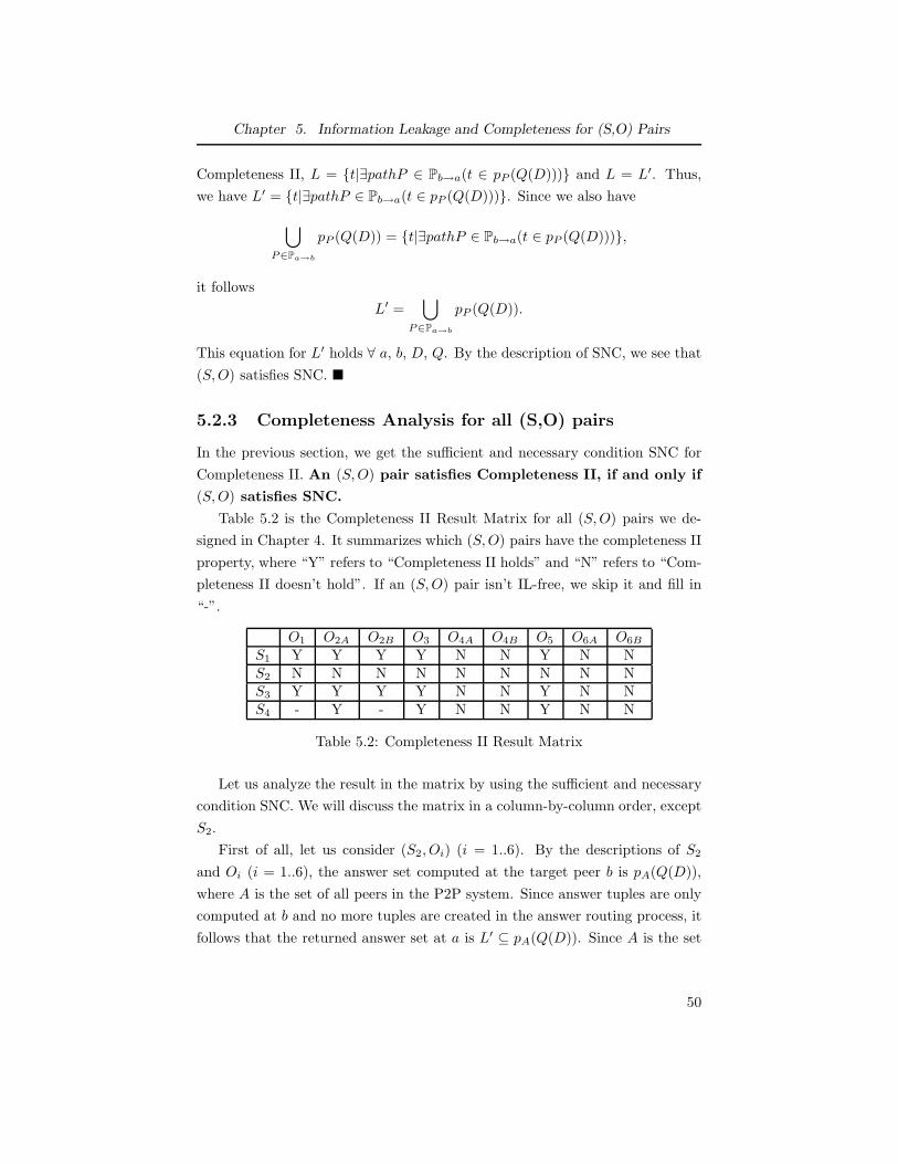
Chapter 5. Information Leakage and Completeness for (S,O) Pairs
Completeness II, L = {t|∃pathP ∈ Pb→a(t ∈ pP (Q(D)))} and L = L′. Thus,
we have L′ = {t|∃pathP ∈ Pb→a(t ∈ pP (Q(D)))}. Since we also have
⋃
P∈Pa→b
pP (Q(D)) = {t|∃pathP ∈ Pb→a(t ∈ pP (Q(D)))},
it follows
L′ =⋃
P∈Pa→b
pP (Q(D)).
This equation for L′ holds ∀ a, b, D, Q. By the description of SNC, we see that
(S, O) satisfies SNC. �
5.2.3 Completeness Analysis for all (S,O) pairs
In the previous section, we get the sufficient and necessary condition SNC for
Completeness II. An (S, O) pair satisfies Completeness II, if and only if
(S, O) satisfies SNC.
Table 5.2 is the Completeness II Result Matrix for all (S, O) pairs we de-
signed in Chapter 4. It summarizes which (S, O) pairs have the completeness II
property, where “Y” refers to “Completeness II holds” and “N” refers to “Com-
pleteness II doesn’t hold”. If an (S, O) pair isn’t IL-free, we skip it and fill in
“-”.
O1 O2A O2B O3 O4A O4B O5 O6A O6B
S1 Y Y Y Y N N Y N NS2 N N N N N N N N NS3 Y Y Y Y N N Y N NS4 - Y - Y N N Y N N
Table 5.2: Completeness II Result Matrix
Let us analyze the result in the matrix by using the sufficient and necessary
condition SNC. We will discuss the matrix in a column-by-column order, except
S2.
First of all, let us consider (S2, Oi) (i = 1..6). By the descriptions of S2
and Oi (i = 1..6), the answer set computed at the target peer b is pA(Q(D)),
where A is the set of all peers in the P2P system. Since answer tuples are only
computed at b and no more tuples are created in the answer routing process, it
follows that the returned answer set at a is L′ ⊆ pA(Q(D)). Since A is the set
50
Chapter 5. Information Leakage and Completeness for (S,O) Pairs
of all peers in the PDMS, normally we have
pA(Q(D)) ⊂⋃
P∈Pa→b
pP (Q(D)).
Since L′ ⊆ pA(Q(D)) and
pA(Q(D)) ⊂⋃
P∈Pa→b
pP (Q(D)),
it follows
L′ ⊂⋃
P∈Pa→b
pP (Q(D)).
Therefore, (S2, Oi) (i = 1..6) doesn’t satisfy SNC.
Let us consider (S1, O1) and (S3, O1). By the descriptions of S1, S3 and
O1, ∀ path P ∈ Pa→b: the answer set at b is pP (Q(D)). Then by O1, ∀ path
P ∈ Pa→b: the answer set pP (Q(D)) is routed at a via the reversed path of P .
Thus, the returned answer set L′ at a is
⋃
P∈Pa→b
pP (Q(D)).
Therefore, (S1, O1) and (S3, O1) satisfy SNC.
Let us consider (Si, O2A) (i = 1, 3, 4). By the descriptions of Si (i = 1, 3, 4)
and O2A, ∀ path P ∈ Pa→b: the answer set at b is pP (Q(D)). Then by O2A,
∀ path P ∈ Pa→b: the answer set pP (Q(D)) is routed at a via some path P ′,
where P ′ ∈ Pb→a ∧ P ′ ⊆ P . Thus, the returned answer set L′ at a is
⋃
P∈Pa→b
pP (Q(D)).
Therefore, (Si, O2A) (i = 1, 3, 4) satisfy SNC.
Let us consider (Si, O2B) (i = 1, 3). Analyzing the case exactly as (Si, O2A)
(i = 1, 3, 4), we will get that (Si, O2B) (i = 1, 3) satisfies SNC.
Let us consider (Si, O3) (i = 1, 3, 4). By the descriptions of Si (i = 1, 3, 4)
and O3, ∀ path P ∈ Pa→b: the answer set at b is pP (Q(D)), annotated with a
safe peer list L. Then by O3, ∀ path P ∈ Pa→b: the answer set pP (Q(D)) is
routed at a via some path P ′, where P ′ ∈ Pb→a ∧ P ′ ⊆ L. (Hint: In the worst
case, P ′ could be the reversed path of P , because P ⊆ L. ) Thus, the returned
51
Chapter 5. Information Leakage and Completeness for (S,O) Pairs
answer set L′ at a is ⋃
P∈Pa→b
pP (Q(D)).
Therefore, (Si, O3) (i = 1, 3, 4) satisfy SNC.
Let us consider (Si, O4A) (i = 1, 3, 4). By the descriptions of Si (i = 1, 3, 4)
and O4A, ∀ path P ∈ Pa→b: the answer set at b is pP (Q(D)). By O4A, ∀ path
P ∈ Pa→b: the answer set pP (Q(D)) is routed to peer d if pd(pP (Q(D))) =
pP (Q(D)). However, without the help of tuple annotations and supporting
elements, the answer set pP (Q(D)) might be blocked during the routing process.
Thus, the returned answer set at a might be
L′ ⊂⋃
P∈Pa→b
pP (Q(D)).
Therefore, (Si, O4A) (i = 1, 3, 4) doesn’t satisfy SNC.
Let us consider (Si, O4B) (i = 1, 3, 4). The analysis is similar with that
of (Si, O4A) (i = 1, 3, 4). The only difference is as follows. By O4B , ∀ path
P ∈ Pa→b: the answer set pP (Q(D)) ∪ S might be blocked at some peer c,
where S per se cannot be safely accessed by c. Therefore, (Si, O4B) (i = 1, 3, 4)
doesn’t satisfy SNC.
Let us consider (Si, O5) (i = 1, 3). By the descriptions of Si (i = 1, 3) and
O5, ∀ path P ∈ Pa→b: the answer set at b is pP (Q(D)). Then by O5, ∀ path
P ∈ Pa→b: the answer set pP (Q(D)) is partitioned and routed back at a via
some paths. (Hint: In the worst case, pP (Q(D)) cannot be partitioned and is
routed back to a via the reversed path of P .) Thus, the returned answer set L′
at a is ⋃
P∈Pa→b
pP (Q(D)).
Therefore, (Si, O5) (i = 1, 3) satisfy SNC.
Let us consider (S4, O5). By the descriptions of S4 and O5, ∀ path P ∈ Pa→b:
the answer set at b is Q(D). By O5, Q(D) is partitioned and routed. Notice that
only the subset pP (Q(D)) is possible to be routed back to a, where P ∈ Pa→b.
Thus, the returned answer set L′ at a is
⋃
P∈Pa→b
pP (Q(D)).
Therefore, (S4, O5) satisfies SNC.
52
Chapter 5. Information Leakage and Completeness for (S,O) Pairs
Let us consider (Si, O6A) (i = 1, 3). By the descriptions of Si (i = 1, 3)
and O6A, ∀ path P ∈ Pa→b: the answer set at b is pP (Q(D)). By O6A, ∀ path
P ∈ Pa→b: peer c, who has the subset K ⊆ pP (Q(D)), routes pd(K) to peer d.
However, without the help of tuple annotations and supporting elements, some
answer tuples in pP (Q(D)) might be blocked/lost during the routing process.
Thus, the returned answer set at a might be
L′ ⊂⋃
P∈Pa→b
pP (Q(D)).
Therefore, (Si, O6A) (i = 1, 3) doesn’t satisfy SNC.
Let us consider (S4, O6A). By the descriptions of S4 and O6A, ∀ path P ∈
Pa→b: the answer set at b is Q(D). However, by O6A, the problem of no tuple
annotations and no supporting elements still exists. Some answer tuples might
be blocked during the routing process. Therefore, (S4, O6A) doesn’t satisfy SNC.
Let us consider (Si, O6B) (i = 1, 3, 4). It is similar to the case of (Si, O6A)
(i = 1, 3, 4). Even with help of supporting elements, O6B might block/lost
some answer tuples during the routing process, if the supporting elements per
se cannot be safely accessed by a routing peer. Therefore, (Si, O6B) (i = 1, 3, 4)
doesn’t satisfy SNC.
53
Chapter 6
Cost Analysis for (S,O)
pairs
Thus far, we presented the designed strategies and options in Chapter 4, and
the IL-free and Completeness property analysis for all (S, O) pairs in Chapter
5. But the cost related to each (S, O) pair has not been studied.
In this chapter, we build the cost model for an (S, O) pair (Section 6.1),
conduct the cost analysis for all (S, O) pairs (Section 6.2), and compare the
analysis to hypothesize which (S, O) pairs perform the best under which condi-
tions (Section 6.3).
6.1 The Cost Model
A cost model estimates the cost of the query-answering process in a PDMS, in
control of an (S, O) pair. The following are the assumptions for the cost model:
• We only consider the cost for given one source peer and one
target peer. The cost estimation can be extended to a general case with
one source peer and multiple target peers.
• We assume that databases residing on all peers have the same
schema. As mentioned in Section 3.4, the access control issue is or-
thogonal to the issue of schema heterogeneity. Tackling query-answering
among different peer schemas is the main task of previous research work
in PDMSs (Section 2.1), which is beyond the scope of the thesis.
• In the cost model, we do not count in the cost of Answer Gen-
erating, which is the cost for the target peer to compute answer tuples
for a query upon its local database. The reason of not including the cost
lies in that (1) this cost is mandatory for every (S, O) pair, and the costs
54
Chapter 6. Cost Analysis for (S,O) pairs
are similar and nondistinctive, (2) answer generating is a local task, whose
time cost is fairly low comparing to those of the networking transaction.
Under the above assumptions, there are several major tasks in the query
answering process of a PDMS:
• Query Transmitting: transmit a query Q from the source peer a to the
target peer b.
• Query Rewriting: rewrite a query Q using ACPs when it is transmitted
from the source peer a to the target peer b.
• ACP Evaluation: use ACPs to determine if a peer has access to certain
answer tuples.
• Answer Routing: ship answer tuples back to the source peer a.
• ACP Distributing: distribute ACPs from the target peer b to other ap-
propriate peers.
• Annotating: associate every partition of the answer tuples with a specific
annotation.
• Annotation Shipping: ship annotations together with the “pure” answer
tuples back to the source peer a.
Now let us identify the primitive operations and the corresponding cost
unit for each task. In order to find reasonable primitive operations and cost
unit for each major task, the following approximation assumptions need to be
made.
Assumption 1: The numbers of constraints in different ACPs do not differ
too much.
Assumption 2: Using each constraint for a query rewriting will cost approx-
imately constant time.
Assumption 3: Using each constraint as a filter to determine whether a peer
has access to an answer tuple will cost approximately constant time.
Assumption 4: In a PDMS, the time to transmit a message between any two
adjacent peers is approximately constant. Thus, it takes approximately
equal time for a small size message to be transmitted between any two
55
Chapter 6. Cost Analysis for (S,O) pairs
adjacent peers. Of course, networking costs do differ, but they are small
enough that the differences are dominated by the other factors.
Assumption 5: The sizes of different answer tuples do not differ too much.
Assumption 6: The sizes of different ACPs do not differ too much.
Assumption 7: The sizes of different annotations do not differ too much.
Assumption 8: An annotation is in the form of a set of peer ID’s. Insert-
ing/deleting an peer ID into/from an annotation costs approximately con-
stant time.
Assumption 9: The sizes of a query and its rewritten forms do not differ too
much.
Assumption 10: An annotation is directly associated and shipped with a set
of tuples. It requires no supportive structure.
Each of the following cost is the time cost for a major task in the query
answering process of a PDMS.
The Query Transmitting Cost refers to the cost of transmitting a query
Q from the source peer a to the target peer b. According to Assumption 4 and
9, it can be inferred that the cost of shipping a query down one network link
is approximately an constant time. “Shipping a query down one network link”
is then the primitive operation. We identify the cost unit as “query-hop”,
which is the charge associated with the primitive operation. Thus the Query
Transmitting Cost can be measured in terms of query-hops.
The Query Rewriting Cost refers to the cost of rewriting a query Q using
ACPs when it is transmitted from the source peer a to the target peer b in
the framework of an (S, O) pair. According to Assumption 1 and 2, it can be
inferred that rewriting query Q using ACP A1 will cost approximately equal
time to that of rewriting query Q using ACP A2, no matter what Q is, or what
A1 and A2 are. So the primitive operation for query rewriting can be regarded
as “rewriting a query using one ACP”. We identify the cost unit as “qrewrite-
acp”, which is the charge associated with the previous primitive operation.
Thus the Query Rewriting Cost can be measured in terms of qrewrite-acps.
E.g. rewriting 1 query using 100 ACPs costs 100 qrewite-acps, which has the
same cost of rewriting 2 queries using 50 ACPs each.
56
Chapter 6. Cost Analysis for (S,O) pairs
The ACP Evaluation refers to using ACPs to determine if a peer is au-
thorized to access certain answer tuples. It happens in two different places: (1)
when certain answer tuples are to be routed from peer c1 to peer c2, related
ACPs are used at c1 to determine if c2 is authorized to access these answer
tuples, (2) ACPs are used as filters at a peer, usually the target peer, to decide
the set of peers that is authorized to access each answer tuple. According to As-
sumption 1 and 3, it can be inferred that evaluating an ACP over a tuple costs
approximately constant time, no matter how the answer tuple looks like. So the
primitive operation for ACP evaluation is “evaluating an ACP over an answer
tuple to decide the related safe peers”. The cost unit is identified as “acp-eval”,
which is the charge associated with the primitive operation. It’s measured on
a per tuple basis. e.g. if we evaluated 1 ACP over 1000 tuples versus 10 ACPs
over 100 tuples each, both cases incur the same cost: 1000 acp-evals. Thus the
ACP Evaluation Cost can be measured in terms of acp-evals.
The Answer Routing Cost refers to the total cost of shipping answer
tuples back to the source peer. According to Assumption 4 and 5, it can be
inferred that the cost of shipping one answer tuple down one network link is
approximately an constant time. “Shipping one answer tuple down one network
link” is then the primitive operation. We identify the cost unit as “tuple-hop”,
which is the charge associated with the previous primitive operation. Thus the
Answer Routing Cost can be measured in terms of tuple-hops. E.g. if 100
tuples are sent down a path of 10 links, the cost is 1000 tuple-hops, which is
also the same charge if 1 tuple is sent down a path of length 1000. Note that
we are considering the amount of work in the network. Actually it is faster to
send 100 tuples down a path of 10 links than to send 1 tuple down a path of
1000 links. The former does the primitive operations in a concurrent way. In
our cost model, we simply sum up all primitive operations as if they are done
sequentially. Likewise, the assumption applies to the Query Transmitting Cost
and the ACP Distributing Cost.
For certain (S, O) pairs, ACPs need to be distributed from the target peer to
other peers. The ACP Distributing Cost refers to such kind of distributing
cost. According to Assumption 4 and 6, it can be inferred that the cost of
shipping one ACP down one network link could be treated as an approximately
constant time. Thus “shipping one ACP down one network link” is the primitive
operation for ACP Distributing Cost. We identify the cost unit as “acp-hop”,
which is the charge associated with the previous primitive operation. So the
ACP Distributing Cost can be measured in terms of acp-hops. E.g. if 100
57
Chapter 6. Cost Analysis for (S,O) pairs
ACPs are sent down a path of 10 links, the cost we charge is 1000 acp-hops,
which is the same cost if 1 ACPs are sent down a path of length 1000.
The Annotating Cost is the cost of associating every partition of the
answer tuples with a specific annotation. As mentioned in Assumption 8, an
annotation is in the form of a set of peer ID’s. Then the task of annotating refers
to the operations of inserting/deleting peer ID’s into/from annotations. The
primitive operation then can be treated as “insert/delete a peer ID into/from an
annotation”. Such an primitive operation is the atomic step for any annotating
algorithm. It works for both tuple-based and partition-based algorithms, i.e.
an algorithm annotating one tuple at a time or an algorithm annotating a set
of tuples at a time. According to Assumption 8, the cost unit is identified
as “annot-update”, which is the charge associated with the aforementioned
primitive operation. So the Annotating Cost can be measured in terms of annot-
updates. E.g. if we insert 4 peer ID’s into an annotation, then delete 2 peer ID’s
from another annotation, the cost we’d charge is 6 annot-updates. Generally
speaking, in a specific annotating algorithm, the task of annotating is often
interleaved with the following tasks:
• answer generating, i.e. computing answer tuples for a query
• ACP evaluation, i.e. using ACPs as filters to decide the peers that have
access to each answer tuple in the answer set
We ignore the cost of answer generating, as mentioned at the beginning of this
section. For ACP evaluation, it is included in the ACP Evaluation Cost.
In some query-answering algorithms, the annotations are routed together
with the answer tuples. This will increase the workload for the whole network.
This cost is called the Annotation Shipping Cost. According to Assumption
4, 7 and 10, it can be inferred that the cost of shipping one annotation down one
network link can be treated as an approximately constant time. Then “shipping
one annotation down one network link” is the primitive operation. The cost unit
is identified as “annot-hop”, which is the charge associated with the primitive
operation. Thus the Annotation Shipping Cost can be measured in terms of
annot-hops. E.g. if 10 annotations are sent down a path of 4 links, the cost
charged is 40 annot-hops, which has the same cost if 2 annotations are sent
down a path of length 20.
Now we have identified the cost unit for each major task in the cost model.
Although these cost units are different from each other, we can certainly find
58
Chapter 6. Cost Analysis for (S,O) pairs
the relationship for some of them. For instance, “tuple-hop”, “acp-hop” and
“annot-hop” are quite similar. The only difference is the size of “cell” to be
shipped. Coefficients can be assigned to illuminate the relationship:
• 1 tuple-hop = c1 · acp-hop
• 1 acp-hop = c2 · annot-hop
where c1 and c2 are application-specific coefficients. With these relationships,
it is possible to sum up the costs of Answer Routing, ACP Distributing and
Annotation Shipping, which helps us to calculate the best/fastest (S, O) pairs.
6.2 Cost Analysis Result
The cost model in Section 6.1 can be used to assess an (S, O) pair. In this
section, we analyze and compare the costs for every (S, O) pair we already
designed. Each cost presented in this section is for ONE query, ONE source
peer, and ONE target peer. Because IL-free and Completeness are necessary
properties for an (S, O) pair, only (S, O) pairs that are both IL-free and complete
are analyzed in this section.
In the results of this section, we sum up the cost of a major task for each
(S, O) pair, as if the primitive operations in this task are done sequentially. But
in a real PMDS, we can pipeline the primitive operations, then a task takes less
time.
For clarity, we define the following terminology, which is used in later dis-
cussion. Given the PDMS topology, all ACPs, the source peer a, the target peer
b:
• The number of all paths from a to b is |Pa→b|;
• Let N0 be the number of all peers in the PDMS;
• Let path Pi ∈ Pa→b (i = 1, .., |Pa→b|), Ni be the number of peers (except
b) in Pi, or the length of Pi;
• When considering only one routing path in Pa→b (e.g. in S2), we will
use the simplified symbols: P denotes the path, N denotes the number of
peers(except b) in P or the length of P ;
• If cj is a peer, let Xj be the number of the target peer b’s ACPs for cj , dj
be the shortest path from the target peer b to cj ;
59
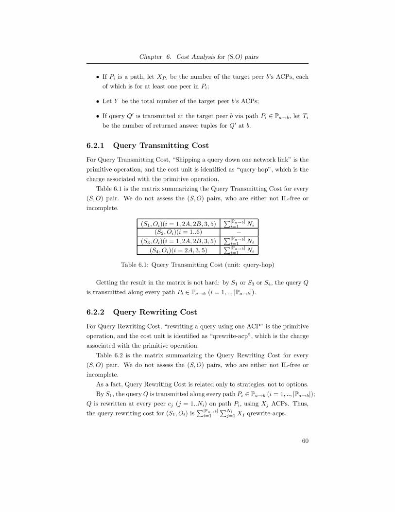
Chapter 6. Cost Analysis for (S,O) pairs
• If Pi is a path, let XPibe the number of the target peer b’s ACPs, each
of which is for at least one peer in Pi;
• Let Y be the total number of the target peer b’s ACPs;
• If query Q′ is transmitted at the target peer b via path Pi ∈ Pa→b, let Ti
be the number of returned answer tuples for Q′ at b.
6.2.1 Query Transmitting Cost
For Query Transmitting Cost, “Shipping a query down one network link” is the
primitive operation, and the cost unit is identified as “query-hop”, which is the
charge associated with the primitive operation.
Table 6.1 is the matrix summarizing the Query Transmitting Cost for every
(S, O) pair. We do not assess the (S, O) pairs, who are either not IL-free or
incomplete.
(S1, Oi)(i = 1, 2A, 2B, 3, 5)∑|Pa→b|
i=1 Ni
(S2, Oi)(i = 1..6) −
(S3, Oi)(i = 1, 2A, 2B, 3, 5)∑|Pa→b|
i=1 Ni
(S4, Oi)(i = 2A, 3, 5)∑|Pa→b|
i=1 Ni
Table 6.1: Query Transmitting Cost (unit: query-hop)
Getting the result in the matrix is not hard: by S1 or S3 or S4, the query Q
is transmitted along every path Pi ∈ Pa→b (i = 1, .., |Pa→b|).
6.2.2 Query Rewriting Cost
For Query Rewriting Cost, “rewriting a query using one ACP” is the primitive
operation, and the cost unit is identified as “qrewrite-acp”, which is the charge
associated with the primitive operation.
Table 6.2 is the matrix summarizing the Query Rewriting Cost for every
(S, O) pair. We do not assess the (S, O) pairs, who are either not IL-free or
incomplete.
As a fact, Query Rewriting Cost is related only to strategies, not to options.
By S1, the query Q is transmitted along every path Pi ∈ Pa→b (i = 1, .., |Pa→b|);
Q is rewritten at every peer cj (j = 1..Ni) on path Pi, using Xj ACPs. Thus,
the query rewriting cost for (S1, Oi) is∑|Pa→b|
i=1
∑Ni
j=1 Xj qrewrite-acps.
60
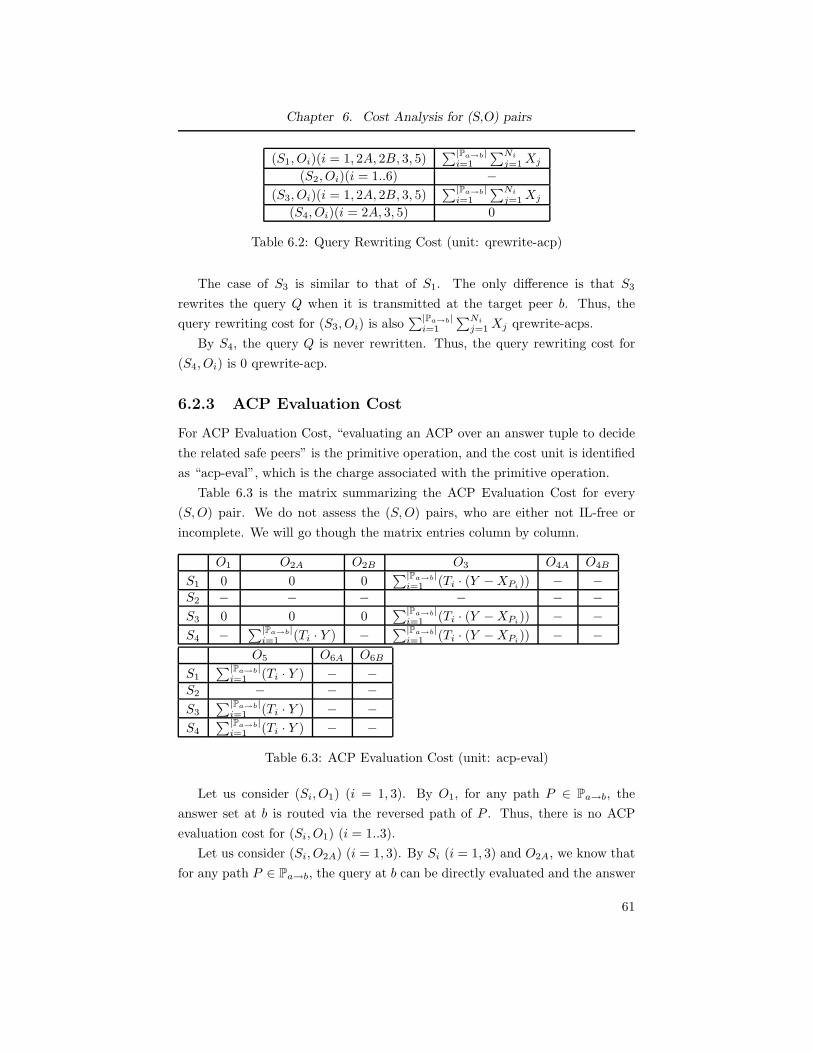
Chapter 6. Cost Analysis for (S,O) pairs
(S1, Oi)(i = 1, 2A, 2B, 3, 5)∑|Pa→b|
i=1
∑Ni
j=1 Xj
(S2, Oi)(i = 1..6) −
(S3, Oi)(i = 1, 2A, 2B, 3, 5)∑|Pa→b|
i=1
∑Ni
j=1 Xj
(S4, Oi)(i = 2A, 3, 5) 0
Table 6.2: Query Rewriting Cost (unit: qrewrite-acp)
The case of S3 is similar to that of S1. The only difference is that S3
rewrites the query Q when it is transmitted at the target peer b. Thus, the
query rewriting cost for (S3, Oi) is also∑|Pa→b|
i=1
∑Ni
j=1 Xj qrewrite-acps.
By S4, the query Q is never rewritten. Thus, the query rewriting cost for
(S4, Oi) is 0 qrewrite-acp.
6.2.3 ACP Evaluation Cost
For ACP Evaluation Cost, “evaluating an ACP over an answer tuple to decide
the related safe peers” is the primitive operation, and the cost unit is identified
as “acp-eval”, which is the charge associated with the primitive operation.
Table 6.3 is the matrix summarizing the ACP Evaluation Cost for every
(S, O) pair. We do not assess the (S, O) pairs, who are either not IL-free or
incomplete. We will go though the matrix entries column by column.
O1 O2A O2B O3 O4A O4B
S1 0 0 0∑|Pa→b|
i=1 (Ti · (Y −XPi)) − −
S2 − − − − − −
S3 0 0 0∑|Pa→b|
i=1 (Ti · (Y −XPi)) − −
S4 −∑|Pa→b|
i=1 (Ti · Y ) −∑|Pa→b|
i=1 (Ti · (Y −XPi)) − −
O5 O6A O6B
S1
∑|Pa→b|i=1 (Ti · Y ) − −
S2 − − −
S3
∑|Pa→b|i=1 (Ti · Y ) − −
S4
∑|Pa→b|i=1 (Ti · Y ) − −
Table 6.3: ACP Evaluation Cost (unit: acp-eval)
Let us consider (Si, O1) (i = 1, 3). By O1, for any path P ∈ Pa→b, the
answer set at b is routed via the reversed path of P . Thus, there is no ACP
evaluation cost for (Si, O1) (i = 1..3).
Let us consider (Si, O2A) (i = 1, 3). By Si (i = 1, 3) and O2A, we know that
for any path P ∈ Pa→b, the query at b can be directly evaluated and the answer
61
Chapter 6. Cost Analysis for (S,O) pairs
set is routed via some path P ′, where P ′ ∈ Pb→a ∧ P ′ ⊆ P . Thus, there is no
ACP evaluation cost for (Si, O2A) (i = 1, 3).
Let us consider (S4, O2A). By S4, for any path P ∈ Pa→b, Q(D) computed
from Q is not exactly pP (Q(D)), which is the answer set O2A will route back.
Thus, O2A needs to evaluate every ACP over every tuple in Q(D) to decide the
returned answer set. Since we know (i) for every path P ∈ Pa→b, the number
of tuples in Q(D) is Ti and (ii) the total number of the target peer’s ACPs is
Y , it follows the ACP evaluation cost is∑|Pa→b|
i=1 (Ti · Y ).
Let us consider (Si, O2B) (i = 1, 3). By O2B , for any path P ∈ Pa→b, the
answer set at b is directly computed by the query Q at b and routed via some
path P ′, where P ′ ∈ Pb→a ∧ P ′ ⊆ P . Thus, there is no ACP evaluation cost
for (Si, O2B) (i = 1, 3).
Let us consider (Si, O3) (i = 1, 3, 4). By O3, for every P ∈ Pa→b, we know (1)
a query Q is transmitted at the target peer b, and the number of answer tuples
is Ti, (2) for each answer tuple t, every ACP of b needs to be evaluated over
t, except the XPiACPs for the peers in Pi (They have been evaluated over t).
Thus, the ACP evaluating cost for (Si, O3) (i = 1, 3, 4) is∑|Pa→b|
i=1 (Ti ·(Y −XPi)).
Let us consider (Si, O5) (i = 1, 3, 4). By O5, we know that for every incoming
path, for every tuple t in the answer set, each ACP of the target peer needs to
be evaluated over t. Thus, the ACP evaluation cost is∑|Pa→b|
i=1 (Ti ·Y ), where Ti
is the number of answer tuples at the target peer and Y is the total number of
the target peer’s ACPs. However, this is the theoretical cost. In practice, the
implementation of O5 may annotate (partition) the answer set before the answer
tuples are computed, and the ACP evaluation cost for (Si, O5) (i = 1, 3, 4) will
decrease dramatically.
6.2.4 Answer Routing Cost
For Answer Routing Cost, “shipping one answer tuple down one network link”
is the primitive operation, and the cost unit is identified as “tuple-hop”, which
is the charge associated with the primitive operation.
Table 6.4 is the matrix summarizing the Answer Routing Cost for every
(S, O) pair. We do not assess the (S, O) pairs, who are either not IL-free or
incomplete. We will go through the matrix entries column by column.
Let us consider (Si, O1) (i = 1, 3). By O1 and Si (i = 1, 3), for any path
Pi ∈ Pa→b, the answer set is returned via the reversed path of Pi. Since the
number of tuples in the answer set is Ti and the length of Pi is Ni, it follows
62
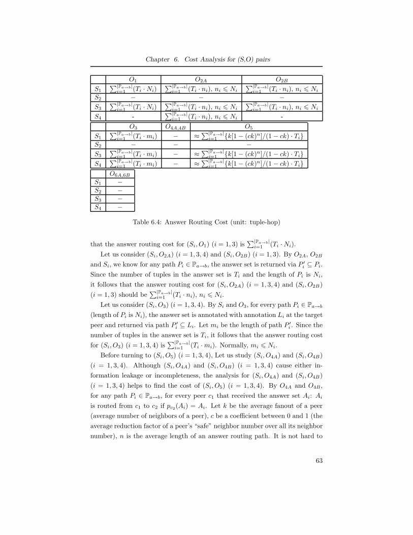
Chapter 6. Cost Analysis for (S,O) pairs
O1 O2A O2B
S1
∑|Pa→b|i=1 (Ti ·Ni)
∑|Pa→b|i=1 (Ti · ni), ni 6 Ni
∑|Pa→b|i=1 (Ti · ni), ni 6 Ni
S2 − − −
S3
∑|Pa→b|i=1 (Ti ·Ni)
∑|Pa→b|i=1 (Ti · ni), ni 6 Ni
∑|Pa→b|i=1 (Ti · ni), ni 6 Ni
S4 -∑|Pa→b|
i=1 (Ti · ni), ni 6 Ni -
O3 O4A,4B O5
S1
∑|Pa→b|i=1 (Ti ·mi) − ≈
∑|Pa→b|i=1 {k[1− (ck)n]/(1− ck) · Ti}
S2 − − −
S3
∑|Pa→b|i=1 (Ti ·mi) − ≈
∑|Pa→b|i=1 {k[1− (ck)n]/(1− ck) · Ti}
S4
∑|Pa→b|i=1 (Ti ·mi) − ≈
∑|Pa→b|i=1 {k[1− (ck)n]/(1− ck) · Ti}
O6A,6B
S1 −S2 −S3 −S4 −
Table 6.4: Answer Routing Cost (unit: tuple-hop)
that the answer routing cost for (Si, O1) (i = 1, 3) is∑|Pa→b|
i=1 (Ti ·Ni).
Let us consider (Si, O2A) (i = 1, 3, 4) and (Si, O2B) (i = 1, 3). By O2A, O2B
and Si, we know for any path Pi ∈ Pa→b, the answer set is returned via P ′i ⊆ Pi.
Since the number of tuples in the answer set is Ti and the length of Pi is Ni,
it follows that the answer routing cost for (Si, O2A) (i = 1, 3, 4) and (Si, O2B)
(i = 1, 3) should be∑|Pa→b|
i=1 (Ti · ni), ni 6 Ni.
Let us consider (Si, O3) (i = 1, 3, 4). By Si and O3, for every path Pi ∈ Pa→b
(length of Pi is Ni), the answer set is annotated with annotation Li at the target
peer and returned via path P ′i ⊆ Li. Let mi be the length of path P ′
i . Since the
number of tuples in the answer set is Ti, it follows that the answer routing cost
for (Si, O3) (i = 1, 3, 4) is∑|Pa→b|
i=1 (Ti ·mi). Normally, mi 6 Ni.
Before turning to (Si, O5) (i = 1, 3, 4), Let us study (Si, O4A) and (Si, O4B)
(i = 1, 3, 4). Although (Si, O4A) and (Si, O4B) (i = 1, 3, 4) cause either in-
formation leakage or incompleteness, the analysis for (Si, O4A) and (Si, O4B)
(i = 1, 3, 4) helps to find the cost of (Si, O5) (i = 1, 3, 4). By O4A and O4B ,
for any path Pi ∈ Pa→b, for every peer c1 that received the answer set Ai: Ai
is routed from c1 to c2 if pc2(Ai) = Ai. Let k be the average fanout of a peer
(average number of neighbors of a peer), c be a coefficient between 0 and 1 (the
average reduction factor of a peer’s “safe” neighbor number over all its neighbor
number), n is the average length of an answer routing path. It is not hard to
63
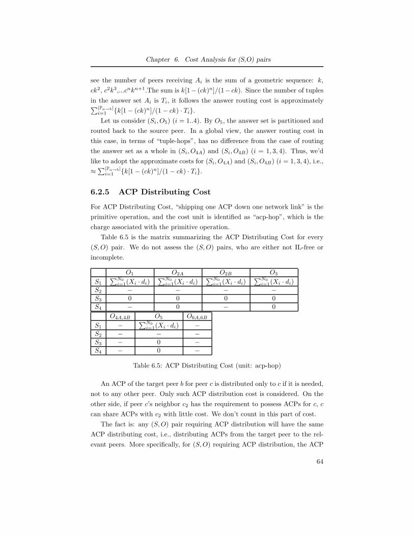
Chapter 6. Cost Analysis for (S,O) pairs
see the number of peers receiving Ai is the sum of a geometric sequence: k,
ck2, c2k3,...cnkn+1.The sum is k[1− (ck)n]/(1− ck). Since the number of tuples
in the answer set Ai is Ti, it follows the answer routing cost is approximately∑|Pa→b|
i=1 {k[1− (ck)n]/(1− ck) · Ti}.
Let us consider (Si, O5) (i = 1..4). By O5, the answer set is partitioned and
routed back to the source peer. In a global view, the answer routing cost in
this case, in terms of “tuple-hops”, has no difference from the case of routing
the answer set as a whole in (Si, O4A) and (Si, O4B) (i = 1, 3, 4). Thus, we’d
like to adopt the approximate costs for (Si, O4A) and (Si, O4B) (i = 1, 3, 4), i.e.,
≈∑|Pa→b|
i=1 {k[1− (ck)n]/(1− ck) · Ti}.
6.2.5 ACP Distributing Cost
For ACP Distributing Cost, “shipping one ACP down one network link” is the
primitive operation, and the cost unit is identified as “acp-hop”, which is the
charge associated with the primitive operation.
Table 6.5 is the matrix summarizing the ACP Distributing Cost for every
(S, O) pair. We do not assess the (S, O) pairs, who are either not IL-free or
incomplete.
O1 O2A O2B O3
S1
∑N0
i=1(Xi · di)∑N0
i=1(Xi · di)∑N0
i=1(Xi · di)∑N0
i=1(Xi · di)S2 − − − −S3 0 0 0 0S4 − 0 − 0
O4A,4B O5 O6A,6B
S1 −∑N0
i=1(Xi · di) −S2 − − −S3 − 0 −S4 − 0 −
Table 6.5: ACP Distributing Cost (unit: acp-hop)
An ACP of the target peer b for peer c is distributed only to c if it is needed,
not to any other peer. Only such ACP distribution cost is considered. On the
other side, if peer c’s neighbor c2 has the requirement to possess ACPs for c, c
can share ACPs with c2 with little cost. We don’t count in this part of cost.
The fact is: any (S, O) pair requiring ACP distribution will have the same
ACP distributing cost, i.e., distributing ACPs from the target peer to the rel-
evant peers. More specifically, for (S, O) requiring ACP distribution, the ACP
64
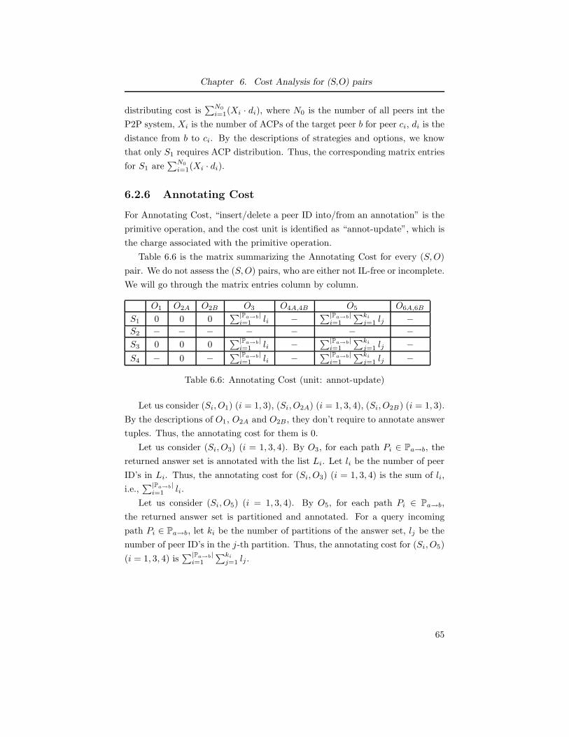
Chapter 6. Cost Analysis for (S,O) pairs
distributing cost is∑N0
i=1(Xi · di), where N0 is the number of all peers int the
P2P system, Xi is the number of ACPs of the target peer b for peer ci, di is the
distance from b to ci. By the descriptions of strategies and options, we know
that only S1 requires ACP distribution. Thus, the corresponding matrix entries
for S1 are∑N0
i=1(Xi · di).
6.2.6 Annotating Cost
For Annotating Cost, “insert/delete a peer ID into/from an annotation” is the
primitive operation, and the cost unit is identified as “annot-update”, which is
the charge associated with the primitive operation.
Table 6.6 is the matrix summarizing the Annotating Cost for every (S, O)
pair. We do not assess the (S, O) pairs, who are either not IL-free or incomplete.
We will go through the matrix entries column by column.
O1 O2A O2B O3 O4A,4B O5 O6A,6B
S1 0 0 0∑|Pa→b|
i=1 li −∑|Pa→b|
i=1
∑ki
j=1 lj −
S2 − − − − − − −
S3 0 0 0∑|Pa→b|
i=1 li −∑|Pa→b|
i=1
∑ki
j=1 lj −
S4 − 0 −∑|Pa→b|
i=1 li −∑|Pa→b|
i=1
∑ki
j=1 lj −
Table 6.6: Annotating Cost (unit: annot-update)
Let us consider (Si, O1) (i = 1, 3), (Si, O2A) (i = 1, 3, 4), (Si, O2B) (i = 1, 3).
By the descriptions of O1, O2A and O2B, they don’t require to annotate answer
tuples. Thus, the annotating cost for them is 0.
Let us consider (Si, O3) (i = 1, 3, 4). By O3, for each path Pi ∈ Pa→b, the
returned answer set is annotated with the list Li. Let li be the number of peer
ID’s in Li. Thus, the annotating cost for (Si, O3) (i = 1, 3, 4) is the sum of li,
i.e.,∑|Pa→b|
i=1 li.
Let us consider (Si, O5) (i = 1, 3, 4). By O5, for each path Pi ∈ Pa→b,
the returned answer set is partitioned and annotated. For a query incoming
path Pi ∈ Pa→b, let ki be the number of partitions of the answer set, lj be the
number of peer ID’s in the j-th partition. Thus, the annotating cost for (Si, O5)
(i = 1, 3, 4) is∑|Pa→b|
i=1
∑ki
j=1 lj .
65
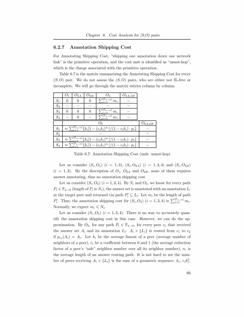
Chapter 6. Cost Analysis for (S,O) pairs
6.2.7 Annotation Shipping Cost
For Annotating Shipping Cost, “shipping one annotation down one network
link” is the primitive operation, and the cost unit is identified as “annot-hop”,
which is the charge associated with the primitive operation.
Table 6.7 is the matrix summarizing the Annotating Shipping Cost for every
(S, O) pair. We do not assess the (S, O) pairs, who are either not IL-free or
incomplete. We will go through the matrix entries column by column.
O1 O2A O2B O3 O4A,4B
S1 0 0 0∑|Pa→b|
i=1 mi −S2 − − − − −
S3 0 0 0∑|Pa→b|
i=1 mi −
S4 − 0 −∑|Pa→b|
i=1 mi −
O5 O6A,6B
S1 ≈∑|Pa→b|
i=1 {ki[1− (ciki)ni ]/(1− ciki) · pi} −
S2 − −
S3 ≈∑|Pa→b|
i=1 {ki[1− (ciki)ni ]/(1− ciki) · pi} −
S4 ≈∑|Pa→b|
i=1 {ki[1− (ciki)ni ]/(1− ciki) · pi} −
Table 6.7: Annotation Shipping Cost (unit: annot-hop)
Let us consider (Si, O1) (i = 1, 3), (Si, O2A) (i = 1, 3, 4) and (Si, O2B)
(i = 1, 3). By the description of O1, O2A and O2B, none of them requires
answer annotating, thus no annotation shipping cost.
Let us consider (Si, O3) (i = 1, 3, 4). By Si and O3, we know for every path
Pi ∈ Pa→b (length of Pi is Ni), the answer set is annotated with an annotation Li
at the target peer and returned via path P ′i ⊆ Li. Let mi be the length of path
P ′i . Thus, the annotation shipping cost for (Si, O3) (i = 1, 3, 4) is
∑|Pa→b|i=1 mi.
Normally, we expect mi 6 Ni.
Let us consider (Si, O5) (i = 1, 3, 4). There is no way to accurately quan-
tify the annotation shipping cost in this case. However, we can do the ap-
proximation. By O5, for any path Pi ∈ Pa→b, for every peer c1 that received
the answer set Ai and its annotation Li: Ai × {Li} is routed from c1 to c2
if pc2(Ai) = Ai. Let ki be the average fanout of a peer (average number of
neighbors of a peer), ci be a coefficient between 0 and 1 (the average reduction
factor of a peer’s “safe” neighbor number over all its neighbor number), ni is
the average length of an answer routing path. It is not hard to see the num-
ber of peers receiving Ai × {Li} is the sum of a geometric sequence: ki, cik2i ,
66
Chapter 6. Cost Analysis for (S,O) pairs
c2i k
3i ,...cni
i kni+1i . The sum is ki[1− (ciki)
ni ]/(1− ciki). Let the number of parti-
tions (annotations) be pi. Thus, the annotation shipping cost is approximately∑|Pa→b|
i=1 {ki[1− (ciki)ni ]/(1− ciki) · pi}.
6.3 Hypothesis for Best (S,O) pairs
Now let us make the hypothesis on which (S, O) pairs are the best in (1) being
IL-free and complete as proved in Chapter 5, (2) fastest one as estimated by
the results in Section 6.2.
First, (S4, O1) and (S4, O2B) are excluded because they are not IL-free.
Besides, (S2, Oj) (j = 1..6), (Si, O4A) (i = 1..4), (Si, O4B) (i = 1..4), (Si, O6A)
(i = 1..4), (Si, O6B) (i = 1..4) are excluded because they are not complete.
Next let us pick out the best (S, O) pairs according to each major cost:
• Query Transmitting Cost is non-discriminative, because this cost for each
(S, O) pair is exactly the same.
• For Query Rewriting Cost, the best (S, O) pairs are (S4, Oi)(i = 2A, 3, 5).
• For ACP Evaluating Cost, the best (S, O) pairs are (S1, Oj) (j = 1, 2A, 2B),
(S3, Oj) (j = 1, 2A, 2B).
• For Answer Routing Cost, the best (S, O) pairs are (Si, O2A) (i = 1, 3, 4)
and (Si, O2B) (i = 1, 3). (Si, O3) (i = 1, 3) cost at the same level of those
best (S, O) pairs.
• For ACP Distributing Cost, the best (S, O) pairs are (S3, Oj)
(j = 1, 2A, 2B, 3, 5) and (S4, Oj) (j = 2A, 3, 5).
• For Annotating Cost, the best (S, O) pairs are (Si, O1) (i = 1, 3), (Si, O2A)
(i = 1, 3, 4) and (Si, O2B) (i = 1, 3).
• For Annotation Shipping Cost, the best (S, O) pairs are (Si, O1) (i = 1, 3),
(Si, O2A) (i = 1, 3, 4) and (Si, O2B) (i = 1, 3).
In the above list, (S3, O2A) and (S3, O2B) are always among the best, except
for the Query Rewriting Cost. As we know, query rewriting is done at peers
locally, and is normally faster than the network transportation, such as query
transmitting and answer routing. Thus, if the local computing speed of peers in
a PDMS is much faster than the network transportation speed, (S3, O2A) and
67
Chapter 6. Cost Analysis for (S,O) pairs
(S3, O2B) perform better than any other (S, O) pair. Notice that when S3 is
used, given source peer a, target peer b, database D at b, query Q that has been
transmitted at b via some path P ∈ Pa→b, we have pP (Q(D)) = Q(D). That
means, (S3, O2A) and (S3, O2B) behave exactly the same. Therefore, if the
local computing speed of peers in a PDMS is much faster than the
network transportation speed, (S3, O2A) is the best (S, O) pair.
Another notable point is: if the local computing speed of peers in a PDMS is
much faster than the network transportation speed, (S3, O2A) may not always be
the best/fastest (S, O) pair. If the local computing speed of peers in a PDMS is
much faster than the network transportation speed, Answer Routing Cost is the
major cost and really matters. From the above bullets, we know that (Si, O3)
(i = 1, 3) perform fairly well at answer routing, though they are not among
the best (S, O) pairs according to most other costs. Given a good PDMS
topology and ACP distribution, (Si, O3) (i = 1, 3) could be the best
(S, O) pairs, even faster than (S3, O2A).
68
Chapter 7
Algorithm Details
We have implemented the strategies and options that can be combined to form
an (S, O) pair being both IL-free and complete. They are S1, S3, S4, O1, O2A,
O2B, O3, and O5. In this chapter, we present the crucial algorithms in these
strategies and options.
7.1 Algorithm for Query-Rewriting in light of
ACPs
By the descriptions of S1 and S3 in Section 4.4, during the query transmitting
process controlled by these two strategies, a query is rewritten into a new query
at some peer to adhere to ACPs defined by the target peer. Therefore, the
algorithm for query-rewriting in light of ACPs plays the central role in S1 and
S3. We present this algorithm in Section 7.1.1, and illustrate it by an example
in Section 7.1.2.
7.1.1 Algorithm Description
Given a query Q and an ACP R, the intuition of the query rewriting algorithm
is to rewrite Q into a new query Q′ such that Q′ satisfies any structure/value
constraint in either Q or R. In another word, for any database, the answer for
Q′ is contained by both the answer for Q and the answer for R, where Q, Q′, R
are treated as tree pattern queries. According to the query containment concept
in Section 2.2, we have Q′ ⊆ Q and Q′ ⊆ R. In our algorithm, the containment
mapping approach is used to ensure these query containment relationships.
First, let us go through some terminology that will be used in the algorithm.
Let Q be a query, R be an ACP. Both Q and R can be expressed as tree pat-
terns. For a tree pattern, there exists an output node that means only instances
corresponding to this output node are returned as the answer set. The output
element in query Q is called return element, and the output element in ACP
69
Chapter 7. Algorithm Details
R is called visible element. There are two types of edges in a tree pattern, i.e.,
pc (parent-child) edge and ad (ancestor-descendant) edge. Secondly, we assume
no more than two nodes in R, or the extension form of R, have the same tag
name. That is the ACP fragment our algorithm currently handles.
The algorithm for Query-Rewriting in light of ACP is shown in Figure 7.1.
Let us explain more on few steps of the algorithm. In step 3 of the algorithm,
it requires that the schema scm is available, at least for all the ancestors and
descendants of visible nodes in TP R. In step 6, it ensures that the nodes in
TP R ext, which are attached with new constraints in step 5 (b), must be in
the range of mapping M . Because the nodes in TP Q ext with the original
constraints are in the domain of M (in fact, every node in TP Q ext is in the
domain of M), thus their mapped nodes in TP R ext to accept these constraints
are in the range of M . So these nodes will not be pruned in step 6 according to
the second condition.
As mentioned earlier, the algorithm ensures Q ⊇ Q′ and R ⊇ Q′. Q ⊇ Q′
because there exists a containment mapping from the tree pattern of Q to the
tree pattern of Q′ (TP R ext), as described in step 5. R ⊇ Q′ because there is
a obvious containment mapping from the tree pattern of R to the tree pattern
of Q′ (TP R ext) since all we’ve done is adding elements to TP R ext.
7.1.2 Example
Let us use an example to illustrate the algorithm in the previous section. In our
example, the output nodes in tree patterns are capitalized.
The database schema scm and the results after each step of the algorithm
are shown in later figures.
After step 1, the corresponding tree patters of given query Q and ACP R are
built. We directly show the tree patterns here, skipping the string expressions
of Q and R.
After step 2, TP R is marked, where marked nodes are tagged with a “*”.
After step 3, TP R is expanded to TP R ext. (Please refer to the schema
scm.)
After step 4, TP Q is expanded to TP Q ext. (Actually nothing changes,
just TP Q has been replicated as TP Q ext.)
Step 5(a) finds the obvious mapping. Because every node in TP Q ext can
be mapped and every edge is preserved. Specially, the “ad” edge “c => b”
in TP Q ext is mapped to a path “c− > g− > f− > b” in TP R ext. The
70
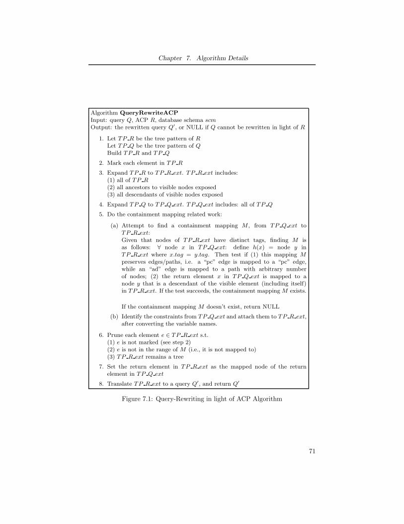
Chapter 7. Algorithm Details
Algorithm QueryRewriteACP
Input: query Q, ACP R, database schema scmOutput: the rewritten query Q′, or NULL if Q cannot be rewritten in light of R
1. Let TP R be the tree pattern of RLet TP Q be the tree pattern of QBuild TP R and TP Q
2. Mark each element in TP R
3. Expand TP R to TP R ext. TP R ext includes:(1) all of TP R(2) all ancestors to visible nodes exposed(3) all descendants of visible nodes exposed
4. Expand TP Q to TP Q ext. TP Q ext includes: all of TP Q
5. Do the containment mapping related work:
(a) Attempt to find a containment mapping M , from TP Q ext toTP R ext:Given that nodes of TP R ext have distinct tags, finding M isas follows: ∀ node x in TP Q ext: define h(x) = node y inTP R ext where x.tag = y.tag. Then test if (1) this mapping Mpreserves edges/paths, i.e. a “pc” edge is mapped to a “pc” edge,while an “ad” edge is mapped to a path with arbitrary numberof nodes; (2) the return element x in TP Q ext is mapped to anode y that is a descendant of the visible element (including itself)in TP R ext. If the test succeeds, the containment mapping M exists.
If the containment mapping M doesn’t exist, return NULL
(b) Identify the constraints from TP Q ext and attach them to TP R ext,after converting the variable names.
6. Prune each element e ∈ TP R ext s.t.(1) e is not marked (see step 2)(2) e is not in the range of M (i.e., it is not mapped to)(3) TP R ext remains a tree
7. Set the return element in TP R ext as the mapped node of the returnelement in TP Q ext
8. Translate TP R ext to a query Q′, and return Q′
Figure 7.1: Query-Rewriting in light of ACP Algorithm
71
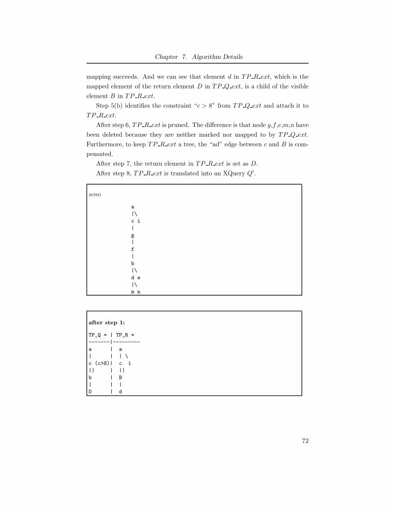
Chapter 7. Algorithm Details
mapping succeeds. And we can see that element d in TP R ext, which is the
mapped element of the return element D in TP Q ext, is a child of the visible
element B in TP R ext.
Step 5(b) identifies the constraint “c > 8” from TP Q ext and attach it to
TP R ext.
After step 6, TP R ext is pruned. The difference is that node g,f ,e,m,n have
been deleted because they are neither marked nor mapped to by TP Q ext.
Furthermore, to keep TP R ext a tree, the “ad” edge between c and B is com-
pensated.
After step 7, the return element in TP R ext is set as D.
After step 8, TP R ext is translated into an XQuery Q′.
scm:
a
|\
c i
|
g
|
f
|
b
|\
d e
|\
m n
after step 1:
TP_Q = | TP_R =
-------|---------
a | a
| | | \
c (c>8)| c i
|| | ||
b | B
| | |
D | d
72
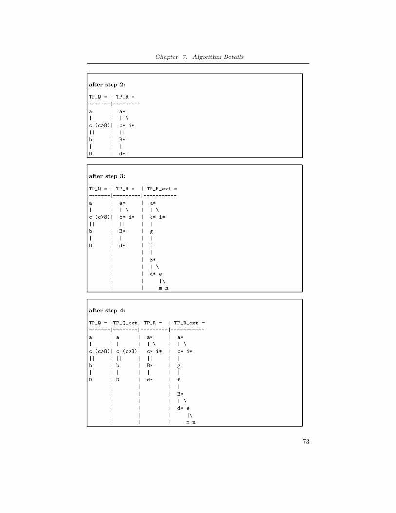
Chapter 7. Algorithm Details
after step 2:
TP_Q = | TP_R =
-------|---------
a | a*
| | | \
c (c>8)| c* i*
|| | ||
b | B*
| | |
D | d*
after step 3:
TP_Q = | TP_R = | TP_R_ext =
-------|---------|-----------
a | a* | a*
| | | \ | | \
c (c>8)| c* i* | c* i*
|| | || | |
b | B* | g
| | | | |
D | d* | f
| | |
| | B*
| | | \
| | d* e
| | |\
| | m n
after step 4:
TP_Q = |TP_Q_ext| TP_R = | TP_R_ext =
-------|--------|---------|-----------
a | a | a* | a*
| | | | | \ | | \
c (c>8)| c (c>8)| c* i* | c* i*
|| | || | || | |
b | b | B* | g
| | | | | | |
D | D | d* | f
| | | |
| | | B*
| | | | \
| | | d* e
| | | |\
| | | m n
73
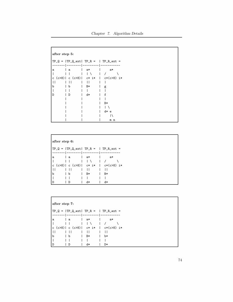
Chapter 7. Algorithm Details
after step 5:
TP_Q = |TP_Q_ext| TP_R = | TP_R_ext =
-------|--------|---------|-----------
a | a | a* | a*
| | | | | \ | / \
c (c>8)| c (c>8)| c* i* | c*(c>8) i*
|| | || | || | |
b | b | B* | g
| | | | | | |
D | D | d* | f
| | | |
| | | B*
| | | | \
| | | d* e
| | | |\
| | | m n
after step 6:
TP_Q = |TP_Q_ext| TP_R = | TP_R_ext =
-------|--------|---------|-----------
a | a | a* | a*
| | | | | \ | / \
c (c>8)| c (c>8)| c* i* | c*(c>8) i*
|| | || | || | ||
b | b | B* | B*
| | | | | | |
D | D | d* | d*
after step 7:
TP_Q = |TP_Q_ext| TP_R = | TP_R_ext =
-------|--------|---------|-----------
a | a | a* | a*
| | | | | \ | / \
c (c>8)| c (c>8)| c* i* | c*(c>8) i*
|| | || | || | ||
b | b | B* | b*
| | | | | | |
D | D | d* | D*
74
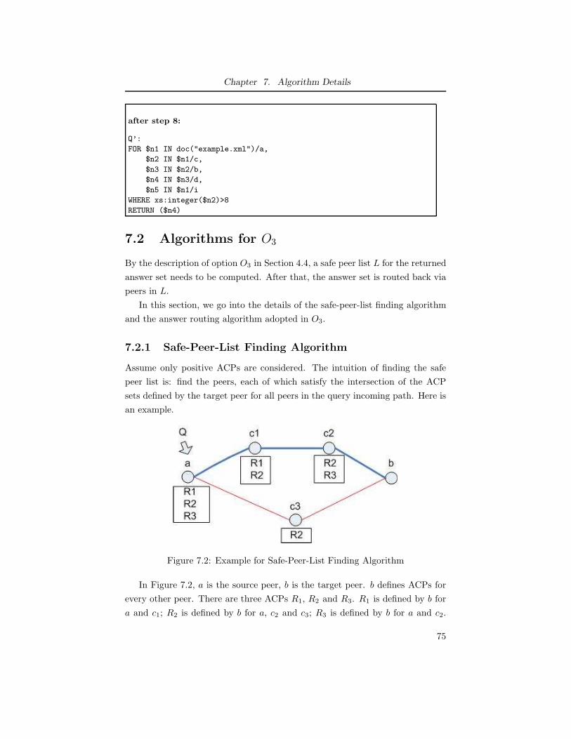
Chapter 7. Algorithm Details
after step 8:
Q’:
FOR $n1 IN doc("example.xml")/a,
$n2 IN $n1/c,
$n3 IN $n2/b,
$n4 IN $n3/d,
$n5 IN $n1/i
WHERE xs:integer($n2)>8
RETURN ($n4)
7.2 Algorithms for O3
By the description of option O3 in Section 4.4, a safe peer list L for the returned
answer set needs to be computed. After that, the answer set is routed back via
peers in L.
In this section, we go into the details of the safe-peer-list finding algorithm
and the answer routing algorithm adopted in O3.
7.2.1 Safe-Peer-List Finding Algorithm
Assume only positive ACPs are considered. The intuition of finding the safe
peer list is: find the peers, each of which satisfy the intersection of the ACP
sets defined by the target peer for all peers in the query incoming path. Here is
an example.
Figure 7.2: Example for Safe-Peer-List Finding Algorithm
In Figure 7.2, a is the source peer, b is the target peer. b defines ACPs for
every other peer. There are three ACPs R1, R2 and R3. R1 is defined by b for
a and c1; R2 is defined by b for a, c2 and c3; R3 is defined by b for a and c2.
75
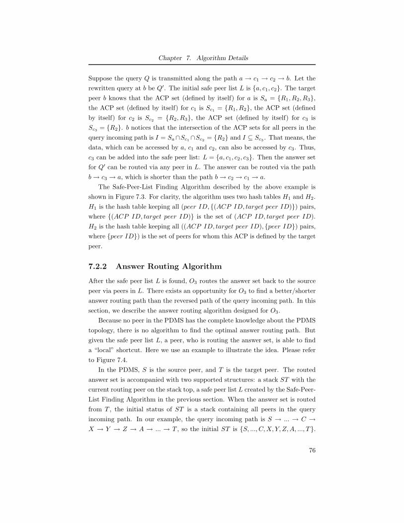
Chapter 7. Algorithm Details
Suppose the query Q is transmitted along the path a → c1 → c2 → b. Let the
rewritten query at b be Q′. The initial safe peer list L is {a, c1, c2}. The target
peer b knows that the ACP set (defined by itself) for a is Sa = {R1, R2, R3},
the ACP set (defined by itself) for c1 is Sc1= {R1, R2}, the ACP set (defined
by itself) for c2 is Sc2= {R2, R3}, the ACP set (defined by itself) for c3 is
Sc3= {R2}. b notices that the intersection of the ACP sets for all peers in the
query incoming path is I = Sa∩Sc1∩Sc2
= {R2} and I ⊆ Sc3. That means, the
data, which can be accessed by a, c1 and c2, can also be accessed by c3. Thus,
c3 can be added into the safe peer list: L = {a, c1, c2, c3}. Then the answer set
for Q′ can be routed via any peer in L. The answer can be routed via the path
b→ c3 → a, which is shorter than the path b→ c2 → c1 → a.
The Safe-Peer-List Finding Algorithm described by the above example is
shown in Figure 7.3. For clarity, the algorithm uses two hash tables H1 and H2.
H1 is the hash table keeping all (peer ID, {(ACP ID, target peer ID)}) pairs,
where {(ACP ID, target peer ID)} is the set of (ACP ID, target peer ID).
H2 is the hash table keeping all ((ACP ID, target peer ID), {peer ID}) pairs,
where {peer ID}) is the set of peers for whom this ACP is defined by the target
peer.
7.2.2 Answer Routing Algorithm
After the safe peer list L is found, O3 routes the answer set back to the source
peer via peers in L. There exists an opportunity for O3 to find a better/shorter
answer routing path than the reversed path of the query incoming path. In this
section, we describe the answer routing algorithm designed for O3.
Because no peer in the PDMS has the complete knowledge about the PDMS
topology, there is no algorithm to find the optimal answer routing path. But
given the safe peer list L, a peer, who is routing the answer set, is able to find
a “local” shortcut. Here we use an example to illustrate the idea. Please refer
to Figure 7.4.
In the PDMS, S is the source peer, and T is the target peer. The routed
answer set is accompanied with two supported structures: a stack ST with the
current routing peer on the stack top, a safe peer list L created by the Safe-Peer-
List Finding Algorithm in the previous section. When the answer set is routed
from T , the initial status of ST is a stack containing all peers in the query
incoming path. In our example, the query incoming path is S → ... → C →
X → Y → Z → A → ... → T , so the initial ST is {S, ..., C, X, Y, Z, A, ..., T}.
76
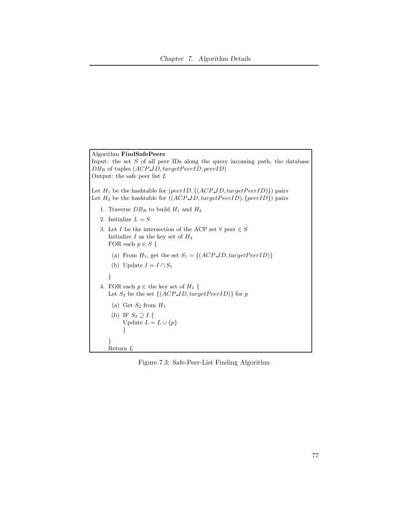
Chapter 7. Algorithm Details
Algorithm FindSafePeers
Input: the set S of all peer IDs along the query incoming path, the databaseDBR of tuples (ACP ID, targetPeerID,peerID)Output: the safe peer list L
Let H1 be the hashtable for (peerID,{(ACP ID, targetPeerID)}) pairsLet H2 be the hashtable for ((ACP ID, targetPeerID),{peerID}) pairs
1. Traverse DBR to build H1 and H2
2. Initialize L = S
3. Let I be the intersection of the ACP set ∀ peer ∈ SInitialize I as the key set of H2
FOR each p ∈ S {
(a) From H1, get the set S1 = {(ACP ID, targetPeerID)}
(b) Update I = I ∩ S1
}
4. FOR each p ∈ the key set of H1 {Let S2 be the set {(ACP ID, targetPeerID)} for p
(a) Get S2 from H1
(b) IF S2 ⊇ I {Update L = L ∪ {p}}
}Return L
Figure 7.3: Safe-Peer-List Finding Algorithm
77
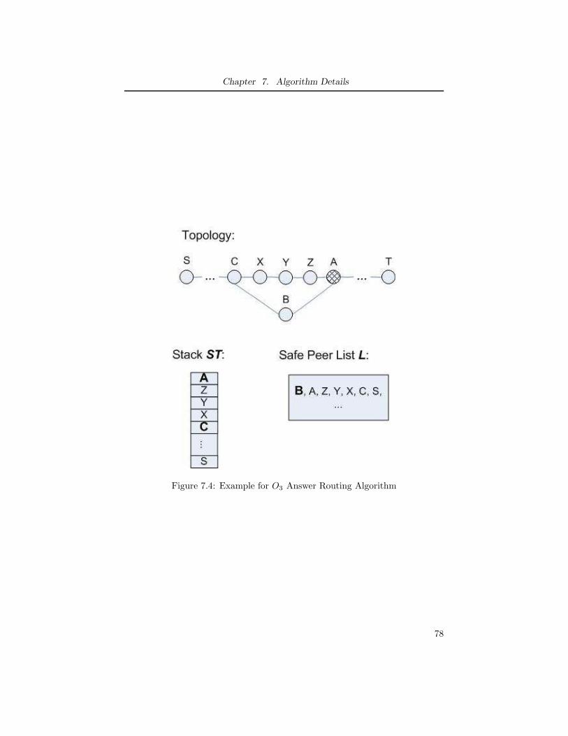
Chapter 7. Algorithm Details
Figure 7.4: Example for O3 Answer Routing Algorithm
78
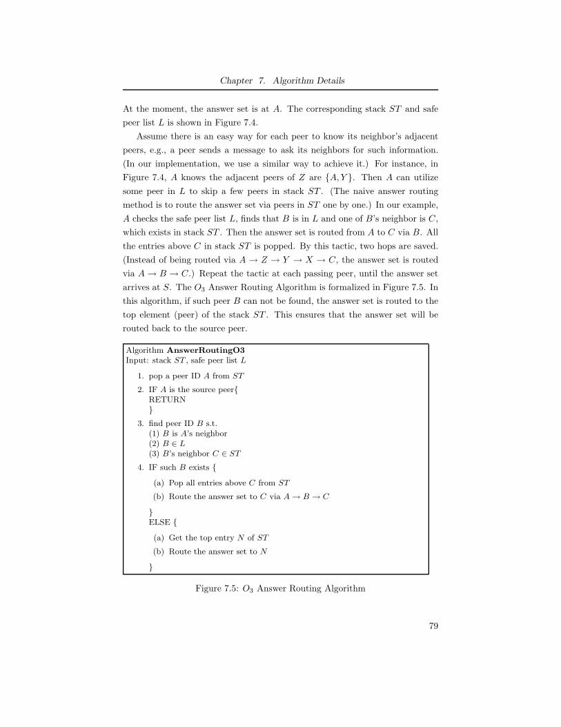
Chapter 7. Algorithm Details
At the moment, the answer set is at A. The corresponding stack ST and safe
peer list L is shown in Figure 7.4.
Assume there is an easy way for each peer to know its neighbor’s adjacent
peers, e.g., a peer sends a message to ask its neighbors for such information.
(In our implementation, we use a similar way to achieve it.) For instance, in
Figure 7.4, A knows the adjacent peers of Z are {A, Y }. Then A can utilize
some peer in L to skip a few peers in stack ST . (The naive answer routing
method is to route the answer set via peers in ST one by one.) In our example,
A checks the safe peer list L, finds that B is in L and one of B’s neighbor is C,
which exists in stack ST . Then the answer set is routed from A to C via B. All
the entries above C in stack ST is popped. By this tactic, two hops are saved.
(Instead of being routed via A → Z → Y → X → C, the answer set is routed
via A→ B → C.) Repeat the tactic at each passing peer, until the answer set
arrives at S. The O3 Answer Routing Algorithm is formalized in Figure 7.5. In
this algorithm, if such peer B can not be found, the answer set is routed to the
top element (peer) of the stack ST . This ensures that the answer set will be
routed back to the source peer.
Algorithm AnswerRoutingO3
Input: stack ST , safe peer list L
1. pop a peer ID A from ST
2. IF A is the source peer{RETURN}
3. find peer ID B s.t.(1) B is A’s neighbor(2) B ∈ L(3) B’s neighbor C ∈ ST
4. IF such B exists {
(a) Pop all entries above C from ST
(b) Route the answer set to C via A→ B → C
}ELSE {
(a) Get the top entry N of ST
(b) Route the answer set to N
}
Figure 7.5: O3 Answer Routing Algorithm
79
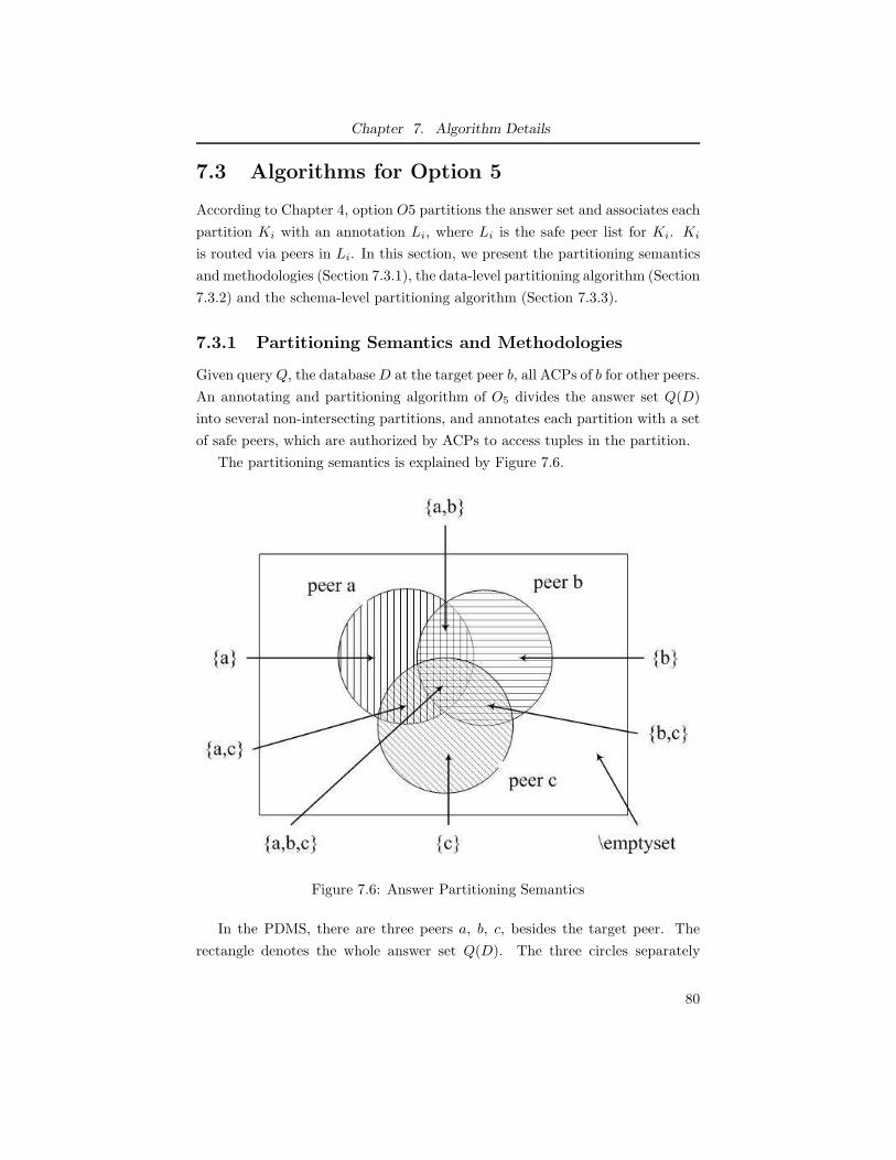
Chapter 7. Algorithm Details
7.3 Algorithms for Option 5
According to Chapter 4, option O5 partitions the answer set and associates each
partition Ki with an annotation Li, where Li is the safe peer list for Ki. Ki
is routed via peers in Li. In this section, we present the partitioning semantics
and methodologies (Section 7.3.1), the data-level partitioning algorithm (Section
7.3.2) and the schema-level partitioning algorithm (Section 7.3.3).
7.3.1 Partitioning Semantics and Methodologies
Given query Q, the database D at the target peer b, all ACPs of b for other peers.
An annotating and partitioning algorithm of O5 divides the answer set Q(D)
into several non-intersecting partitions, and annotates each partition with a set
of safe peers, which are authorized by ACPs to access tuples in the partition.
The partitioning semantics is explained by Figure 7.6.
Figure 7.6: Answer Partitioning Semantics
In the PDMS, there are three peers a, b, c, besides the target peer. The
rectangle denotes the whole answer set Q(D). The three circles separately
80
Chapter 7. Algorithm Details
denote the set of answer tuples that can be accessed by a, b, c, according to the
ACPs defined by the target peer. As we see, the answer set Q(D) is divided
into eight non-intersecting partitions, separately attached with annotations {a},
{b}, {c}, {a, b}, {a, c}, {b, c}, {a, b, c}, ∅. Each partition is maximized and its
annotation set is maximized. More specifically, after partitioning, every answer
tuple t ∈ Q(D) is put into a partition that has an annotation S, such that S is
the maximum set of safe peers for t. This is the semantics for partitioning and
annotating.
There are two possible methods of conducting the annotating and partition-
ing:
Method 1. Interleave ACP checking with evaluation of Q(D). In another
words, whenever computing an answer tuple according to Q and an ACP,
modify this tuple’s annotation. After all tuples have been computed and
annotated, partition them according to their annotations.
Method 2. First evaluate Q(D) and get the answer set. Then find an algo-
rithm for checking all ACPs on all the answer tuples and annotating them.
Finally partition tuples according to their annotations.
Method 2 relies on the supporting elements, which might have been projected
out but are required to be kept in the answer tuples of Q(D). However, Method 1
doesn’t have such a restriction. So we choose to use Method 1 in our partitioning
algorithm.
There are two types of ACPs: data-level and schema-level ACPs. Data-
level ACPs do not affect the schema of answer tuples, which all adhere to the
same schema; while schema-level ACPs will project on some elements and thus
affect the schema of answer tuples. We will work on the data-level partitioning
algorithm in Section 7.3.2 and the schema-level partitioning algorithm in Section
7.3.3.
7.3.2 Data-level Partitioning Algorithm
Assume all ACPs defined by the target peer are data-level ACPs. Then ACPs do
not affect the schema of answer tuples. Therefore, it is easy to check if an answer
tuple exists in an answer set. From this conclusion, the intuition of our data-
level partitioning algorithm is as follows. Initialize the answer set as an empty
set. Each ACP is independently combined with the original query to compute
answer tuples. For each computed answer tuple, check whether it exists in the
81
Chapter 7. Algorithm Details
current answer set. If so, we expand its annotation to include peers associated
with the current ACP; else we add the tuple to the answer set, annotating with
peers associated with the current ACP. After the process, the annotation of each
answer tuple is maximized. Then according to their annotations, the tuples can
be grouped to form proper partitions, which have the same property as Figure
7.6. The Data-level Partitioning Algorithm is shown in Figure 7.7.
In Algorithm DataLevelPartition, step 1 and step 2 are responsible for
computing and annotating answer tuples, step 3 call Procedure Grouping to
form partitions. Procedure Grouping traverses the annotated answer tuples
once and groups them into several partitions. Any tuple t is put into a partition
with the same annotation of t.
7.3.3 Schema-level Partitioning Algorithm
The partitioning algorithm in the previous section can only handle data-level
ACPs. Now let us extend the algorithm to tackle both data-level and schema-
level ACPs.
In order to partition answer tuples in different schemas, we must have a clear
idea on what an answer tuple schema and an answer tuple are. An answer tuple
schema is the schema of an answer tuple. It is a set of attributes. An answer
tuple is a set of attribute values. More specifically, in a relational query, each
answer tuple is a set of table attribute values; in an XQuery, each answer tuple
is a set of user-defined variable values , if not considering result restructuring.
There is a useful relationship between two answer tuples in different schemas.
We define it as a new operator, Tuple Containment :
Definition 7.1 (Tuple Containment) Let T1 be an answer tuple and S1 be
T1’s schema. Given an attribute value v ∈ T1, v.attrS1 is v’s corresponding
attribute ∈ S1. Let T2 be an answer tuple and S2 be T2’s schema. Given an
attribute value v ∈ T2, v.attrS2 is v’s corresponding attribute ∈ S2. T1 is Tuple-
Contained by T2 if and only if ∀v ∈ T1: ∃v ∈ T2 s.t. v.attrS1 = v.attrS2. It
is written as T1 E T2. If T1 E T2 and S1 ⊂ S2, we say T1 is strictly Tuple-
Contained by T2, written as T1 ⊳ T2.
Here is an example for the Tuple Containment. The schema for answer tuple
t is (A1, A3) and t = (′a′1,
′a′3); the schema for answer tuple t′ is (A1, A2, A3)
and t′=(′a′1,
′a′2,
′a′3). According to the tuple containment definition, we have
t ⊳ t′.
82
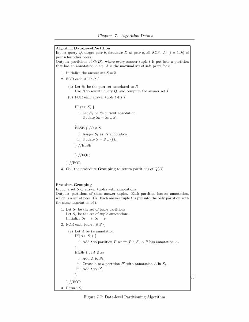
Chapter 7. Algorithm Details
Algorithm DataLevelPartition
Input: query Q, target peer b, database D at peer b, all ACPs Ai (i = 1..k) ofpeer b for other peers.Output: partitions of Q(D), where every answer tuple t is put into a partitionthat has an annotation A s.t. A is the maximal set of safe peers for t.
1. Initialize the answer set S = ∅.
2. FOR each ACP R {
(a) Let S1 be the peer set associated to RUse R to rewrite query Q, and compute the answer set I
(b) FOR each answer tuple t ∈ I {
IF (t ∈ S) {
i. Let S0 be t’s current annotationUpdate S0 = S0 ∪ S1
}ELSE { //t /∈ S
i. Assign S1 as t’s annotation.
ii. Update S = S ∪ {t}.
} //ELSE
} //FOR
} //FOR
3. Call the procedure Grouping to return partitions of Q(D)
Procedure Grouping
Input: a set S of answer tuples with annotationsOutput: partitions of these answer tuples. Each partition has an annotation,which is a set of peer IDs. Each answer tuple t is put into the only partition withthe same annotation of t.
1. Let S1 be the set of tuple partitionsLet S2 be the set of tuple annotationsInitialize S1 = ∅, S2 = ∅
2. FOR each tuple t ∈ S {
(a) Let A be t’s annotationIF(A ∈ S2) {
i. Add t to partition P where P ∈ S1 ∧ P has annotation A.
}ELSE { //A /∈ S2
i. Add A to S2.
ii. Create a new partition P ′ with annotation A in S1.
iii. Add t to P ′.
}
} //FOR
3. Return S1
Figure 7.7: Data-level Partitioning Algorithm
83
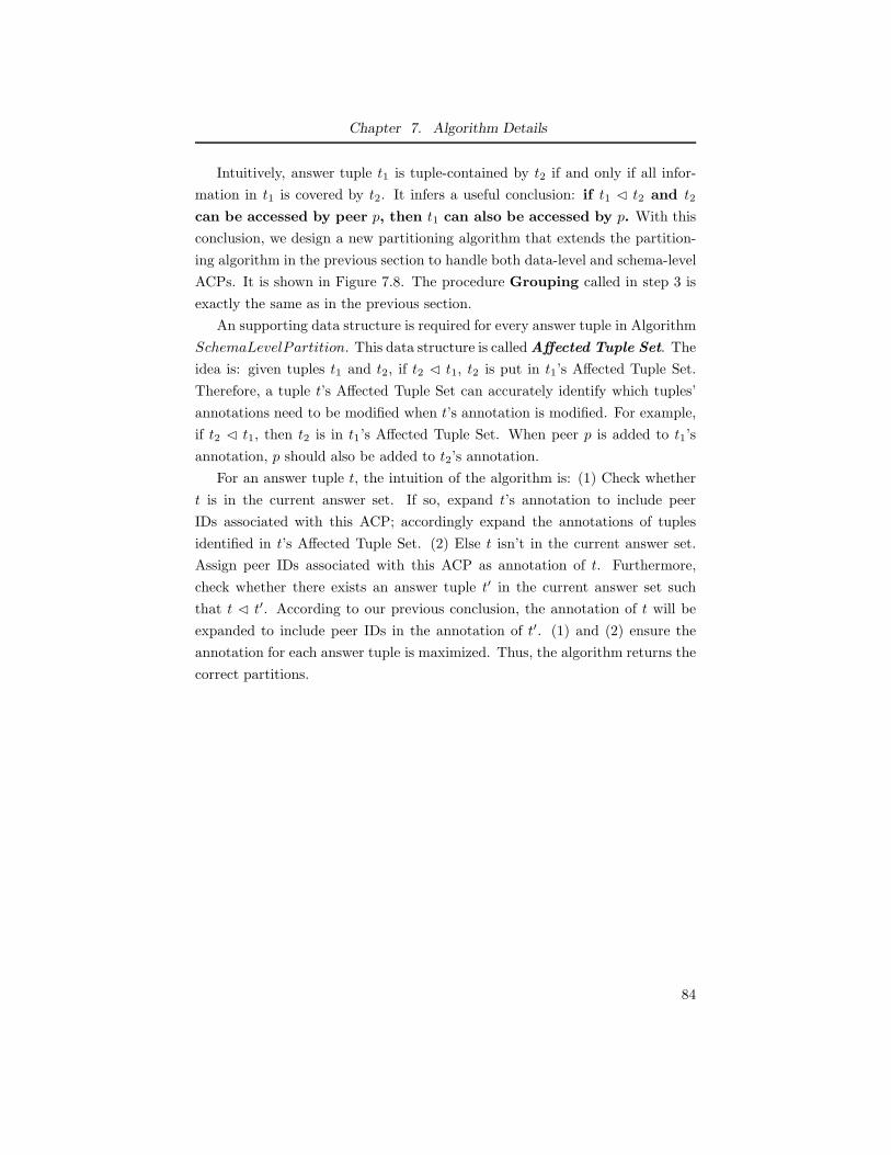
Chapter 7. Algorithm Details
Intuitively, answer tuple t1 is tuple-contained by t2 if and only if all infor-
mation in t1 is covered by t2. It infers a useful conclusion: if t1 ⊳ t2 and t2
can be accessed by peer p, then t1 can also be accessed by p. With this
conclusion, we design a new partitioning algorithm that extends the partition-
ing algorithm in the previous section to handle both data-level and schema-level
ACPs. It is shown in Figure 7.8. The procedure Grouping called in step 3 is
exactly the same as in the previous section.
An supporting data structure is required for every answer tuple in Algorithm
SchemaLevelPartition. This data structure is called Affected Tuple Set. The
idea is: given tuples t1 and t2, if t2 ⊳ t1, t2 is put in t1’s Affected Tuple Set.
Therefore, a tuple t’s Affected Tuple Set can accurately identify which tuples’
annotations need to be modified when t’s annotation is modified. For example,
if t2 ⊳ t1, then t2 is in t1’s Affected Tuple Set. When peer p is added to t1’s
annotation, p should also be added to t2’s annotation.
For an answer tuple t, the intuition of the algorithm is: (1) Check whether
t is in the current answer set. If so, expand t’s annotation to include peer
IDs associated with this ACP; accordingly expand the annotations of tuples
identified in t’s Affected Tuple Set. (2) Else t isn’t in the current answer set.
Assign peer IDs associated with this ACP as annotation of t. Furthermore,
check whether there exists an answer tuple t′ in the current answer set such
that t ⊳ t′. According to our previous conclusion, the annotation of t will be
expanded to include peer IDs in the annotation of t′. (1) and (2) ensure the
annotation for each answer tuple is maximized. Thus, the algorithm returns the
correct partitions.
84
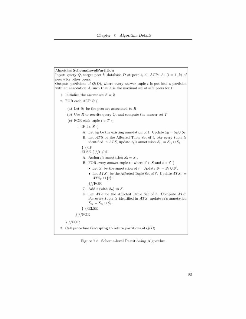
Chapter 7. Algorithm Details
Algorithm SchemaLevelPartition
Input: query Q, target peer b, database D at peer b, all ACPs Ai (i = 1..k) ofpeer b for other peers.Output: partitions of Q(D), where every answer tuple t is put into a partitionwith an annotation A, such that A is the maximal set of safe peers for t.
1. Initialize the answer set S = ∅.
2. FOR each ACP R {
(a) Let S1 be the peer set associated to R
(b) Use R to rewrite query Q, and compute the answer set T
(c) FOR each tuple t ∈ T {
i. IF t ∈ S {
A. Let S0 be the existing annotation of t. Update S0 = S0 ∪S1.
B. Let ATS be the Affected Tuple Set of t. For every tuple t1identified in ATS, update t1’s annotation St1
= St1∪ S1.
} //IFELSE { //t /∈ S
A. Assign t’s annotation S0 = S1.
B. FOR every answer tuple t′, where t′ ∈ S and t ⊳ t′ {
• Let S′ be the annotation of t′. Update S0 = S0 ∪ S′.
• Let ATSt′ be the Affected Tuple Set of t′. Update ATSt′ =ATSt′ ∪ {t}.
}//FOR
C. Add t (with S0) to S.
D. Let ATS be the Affected Tuple Set of t. Compute ATS.For every tuple t1 identified in ATS, update t1’s annotationSt1
= St1∪ S0.
} //ELSE
} //FOR
} //FOR
3. Call procedure Grouping to return partitions of Q(D)
Figure 7.8: Schema-level Partitioning Algorithm
85
Chapter 8
Experimental Study
In Chapter 3, we introduced the information leakage and completeness problems
of the query answering process in a PDMS with access control requirements.
Then in Chapter 4, our solution for the problem was presented: we designed
some strategies and options to handle access control. Furthermore, we built a
cost model to theoretically analyze the cost for each (S, O) pair that ensures IL-
free and completeness in Chapter 6, where a hypothesis for best/fastest (S, O)
pairs are proposed by us.
In this chapter, we use experiments to verify our hypothesis for best (S, O)
pairs, and study the algorithm scalability. Specifically, we describe the experi-
ment implementation in Section 8.1, compare the running time of (S, O) pairs
in Section 8.2, and study the scalability in different facets in Section 8.3.
8.1 Experimental Settings and Implementation
To setup the P2P networking environment, FreePastry [3] is used in our ex-
periment. FreePastry is an open-source P2P overlay network implementation.
It provides an efficient algorithm for message routing, whose complexity is
O(logN), where N is the number of nodes in the network. Moreover, user-
specified applications can be easily integrated with existing FreePastry source
codes. In our experiment, FreePastry version 1.4.4 is used.
As to the emulation test bed, Emulab [2] is adopted in our experiment.
Emulab holds a collection of hundreds of PCs for allocation. For an experiment
at Emulab, the user can freely specify the topology of a network, the type of
PCs in the network, latency, bandwidth, and so on. During the experiment life
cycle, the user has full control on the allocated PCs. Thus, user applications
can be loaded on any PC in the experiment. In our experiment, 47 PCs in
Emulab are required and allocated: 31 of them work as peers in a PDMS, and
the remaining 16 as the delay nodes that controls the networking traffic shaping.
Unless specified otherwise, in later experiments, the network bandwidth is 50
86
Chapter 8. Experimental Study
MB, the latency is 100 ms. The bandwidth is big enough to avoid the bottleneck,
comparing with the size of query/answer messages (at most few KB each). Every
PC allocated has 3.0 GHz 64-bit Xeon processor and 2 GB RAM, with Testbed
version of RedHat Linux 9.0 as the operating system. Our PDMS application
built on FreePastry and the database are loaded on each PC.
To the best of our knowledge, Qizx [4] is the fastest open-source Java XML
query engine. So it is used in our experiment for peers to query their local XML
databases. Qizx supports the standard XQuery language, and also provides
Java APIs to invoke the XQuery engine. In our experiment, Qizx version 1.0 is
used.
In order to make the XML databases on peers general enough, we choose
XMark [1] data generator to randomly create XML data. XMark project pro-
vides a benchmark suite for users. The XMark data generator can produce
random XML documents modeling an auction website. Important structure
features in a typical XML document is included in an XMark-created XML
document. In our experiment, we create several XML databases, whose sizes
range from 10 Mb to 40 Mb.
We manually build the schema for Xmark-created XML databases and a
library of 20 ACPs. We design a topology generator to randomly create the
PDMS topology we need. All the strategies and options, which can be combined
while keeping IL-free and Completeness properties, are implemented. The peer
application, which specifies its strategy and the option, is loaded on each PC
(peer) allocated by Emulab.
Our implementation is written in Java 1.5 to make it cross-platform.
8.2 (S, O) Pair Comparison and Analysis
In this section, we experiment to compare the running time of the query-
answering process controlled by (S, O) pairs that are both IL-free and complete.
The running time here and in the next section is for ONE source peer, ONE
target peer and ONE query, which adheres to the setting of the theoretical
cost analysis for an (S, O) pair (Chapter 6). The first reason lies in that using
the same setting, the experiment result can directly verify our theoretical cost
analysis and hypothesis. The second reason is that the result for one query,
one source peer and one target peer can be extended to a general case with
one query, one source peer and multiple target peers, which doesn’t violate our
87
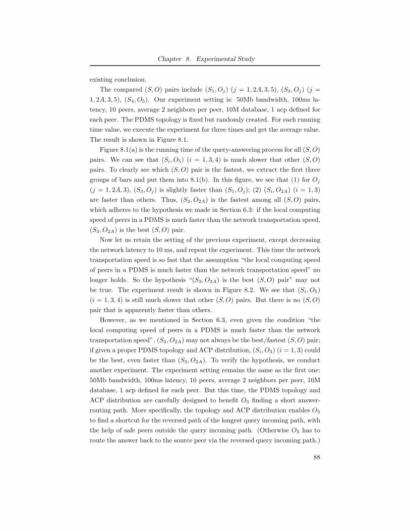
Chapter 8. Experimental Study
existing conclusion.
The compared (S, O) pairs include (S1, Oj) (j = 1, 2A, 3, 5), (S3, Oj) (j =
1, 2A, 3, 5), (S4, O5). Our experiment setting is: 50Mb bandwidth, 100ms la-
tency, 10 peers, average 2 neighbors per peer, 10M database, 1 acp defined for
each peer. The PDMS topology is fixed but randomly created. For each running
time value, we execute the experiment for three times and get the average value.
The result is shown in Figure 8.1.
Figure 8.1(a) is the running time of the query-answering process for all (S, O)
pairs. We can see that (Si, O5) (i = 1, 3, 4) is much slower that other (S, O)
pairs. To clearly see which (S, O) pair is the fastest, we extract the first three
groups of bars and put them into 8.1(b). In this figure, we see that (1) for Oj
(j = 1, 2A, 3), (S3, Oj) is slightly faster than (S1, Oj); (2) (Si, O2A) (i = 1, 3)
are faster than others. Thus, (S3, O2A) is the fastest among all (S, O) pairs,
which adheres to the hypothesis we made in Section 6.3: if the local computing
speed of peers in a PDMS is much faster than the network transportation speed,
(S3, O2A) is the best (S, O) pair.
Now let us retain the setting of the previous experiment, except decreasing
the network latency to 10 ms, and repeat the experiment. This time the network
transportation speed is so fast that the assumption “the local computing speed
of peers in a PDMS is much faster than the network transportation speed” no
longer holds. So the hypothesis “(S3, O2A) is the best (S, O) pair” may not
be true. The experiment result is shown in Figure 8.2. We see that (Si, O5)
(i = 1, 3, 4) is still much slower that other (S, O) pairs. But there is no (S, O)
pair that is apparently faster than others.
However, as we mentioned in Section 6.3, even given the condition “the
local computing speed of peers in a PDMS is much faster than the network
transportation speed”, (S3, O2A) may not always be the best/fastest (S, O) pair;
if given a proper PDMS topology and ACP distribution, (Si, O3) (i = 1, 3) could
be the best, even faster than (S3, O2A). To verify the hypothesis, we conduct
another experiment. The experiment setting remains the same as the first one:
50Mb bandwidth, 100ms latency, 10 peers, average 2 neighbors per peer, 10M
database, 1 acp defined for each peer. But this time, the PDMS topology and
ACP distribution are carefully designed to benefit O3 finding a short answer-
routing path. More specifically, the topology and ACP distribution enables O3
to find a shortcut for the reversed path of the longest query incoming path, with
the help of safe peers outside the query incoming path. (Otherwise O3 has to
route the answer back to the source peer via the reversed query incoming path.)
88
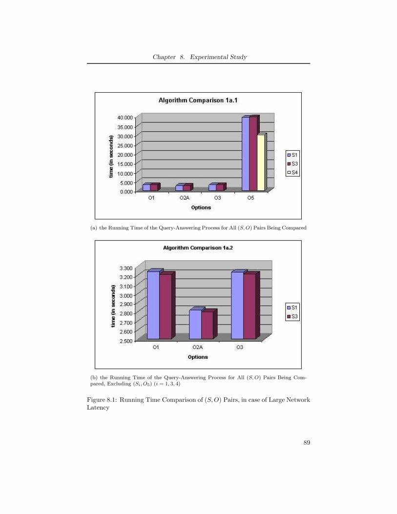
Chapter 8. Experimental Study
(a) the Running Time of the Query-Answering Process for All (S, O) Pairs Being Compared
(b) the Running Time of the Query-Answering Process for All (S, O) Pairs Being Com-pared, Excluding (Si, O5) (i = 1, 3, 4)
Figure 8.1: Running Time Comparison of (S, O) Pairs, in case of Large NetworkLatency
89
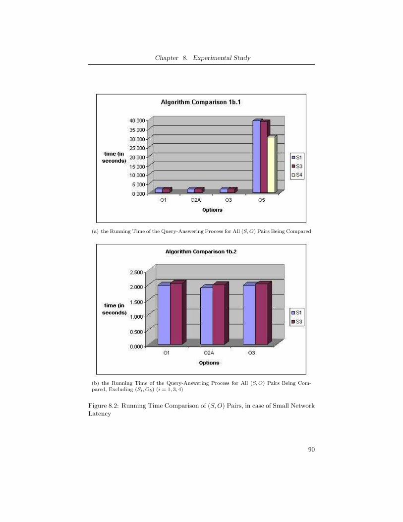
Chapter 8. Experimental Study
(a) the Running Time of the Query-Answering Process for All (S, O) Pairs Being Compared
(b) the Running Time of the Query-Answering Process for All (S, O) Pairs Being Com-pared, Excluding (Si, O5) (i = 1, 3, 4)
Figure 8.2: Running Time Comparison of (S, O) Pairs, in case of Small NetworkLatency
90
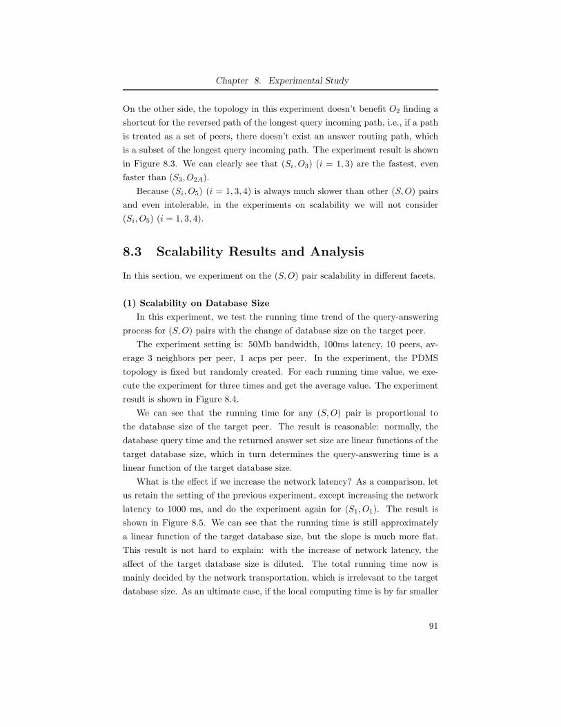
Chapter 8. Experimental Study
On the other side, the topology in this experiment doesn’t benefit O2 finding a
shortcut for the reversed path of the longest query incoming path, i.e., if a path
is treated as a set of peers, there doesn’t exist an answer routing path, which
is a subset of the longest query incoming path. The experiment result is shown
in Figure 8.3. We can clearly see that (Si, O3) (i = 1, 3) are the fastest, even
faster than (S3, O2A).
Because (Si, O5) (i = 1, 3, 4) is always much slower than other (S, O) pairs
and even intolerable, in the experiments on scalability we will not consider
(Si, O5) (i = 1, 3, 4).
8.3 Scalability Results and Analysis
In this section, we experiment on the (S, O) pair scalability in different facets.
(1) Scalability on Database Size
In this experiment, we test the running time trend of the query-answering
process for (S, O) pairs with the change of database size on the target peer.
The experiment setting is: 50Mb bandwidth, 100ms latency, 10 peers, av-
erage 3 neighbors per peer, 1 acps per peer. In the experiment, the PDMS
topology is fixed but randomly created. For each running time value, we exe-
cute the experiment for three times and get the average value. The experiment
result is shown in Figure 8.4.
We can see that the running time for any (S, O) pair is proportional to
the database size of the target peer. The result is reasonable: normally, the
database query time and the returned answer set size are linear functions of the
target database size, which in turn determines the query-answering time is a
linear function of the target database size.
What is the effect if we increase the network latency? As a comparison, let
us retain the setting of the previous experiment, except increasing the network
latency to 1000 ms, and do the experiment again for (S1, O1). The result is
shown in Figure 8.5. We can see that the running time is still approximately
a linear function of the target database size, but the slope is much more flat.
This result is not hard to explain: with the increase of network latency, the
affect of the target database size is diluted. The total running time now is
mainly decided by the network transportation, which is irrelevant to the target
database size. As an ultimate case, if the local computing time is by far smaller
91
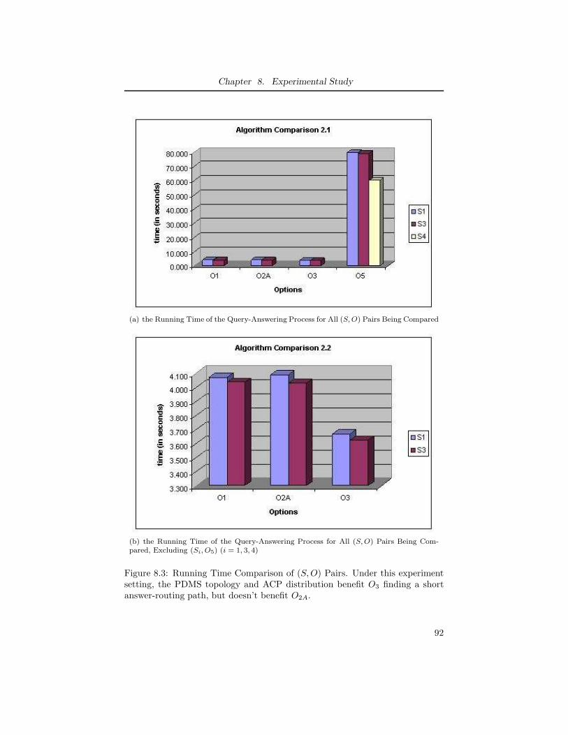
Chapter 8. Experimental Study
(a) the Running Time of the Query-Answering Process for All (S, O) Pairs Being Compared
(b) the Running Time of the Query-Answering Process for All (S, O) Pairs Being Com-pared, Excluding (Si, O5) (i = 1, 3, 4)
Figure 8.3: Running Time Comparison of (S, O) Pairs. Under this experimentsetting, the PDMS topology and ACP distribution benefit O3 finding a shortanswer-routing path, but doesn’t benefit O2A.
92
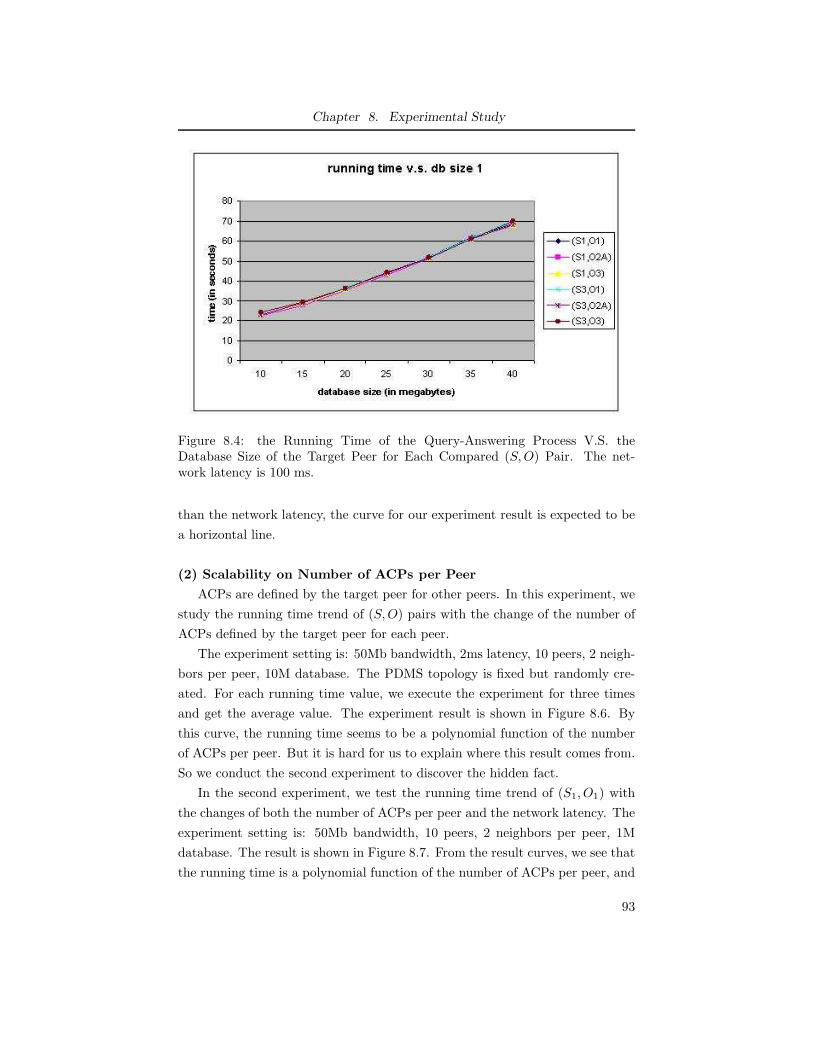
Chapter 8. Experimental Study
Figure 8.4: the Running Time of the Query-Answering Process V.S. theDatabase Size of the Target Peer for Each Compared (S, O) Pair. The net-work latency is 100 ms.
than the network latency, the curve for our experiment result is expected to be
a horizontal line.
(2) Scalability on Number of ACPs per Peer
ACPs are defined by the target peer for other peers. In this experiment, we
study the running time trend of (S, O) pairs with the change of the number of
ACPs defined by the target peer for each peer.
The experiment setting is: 50Mb bandwidth, 2ms latency, 10 peers, 2 neigh-
bors per peer, 10M database. The PDMS topology is fixed but randomly cre-
ated. For each running time value, we execute the experiment for three times
and get the average value. The experiment result is shown in Figure 8.6. By
this curve, the running time seems to be a polynomial function of the number
of ACPs per peer. But it is hard for us to explain where this result comes from.
So we conduct the second experiment to discover the hidden fact.
In the second experiment, we test the running time trend of (S1, O1) with
the changes of both the number of ACPs per peer and the network latency. The
experiment setting is: 50Mb bandwidth, 10 peers, 2 neighbors per peer, 1M
database. The result is shown in Figure 8.7. From the result curves, we see that
the running time is a polynomial function of the number of ACPs per peer, and
93
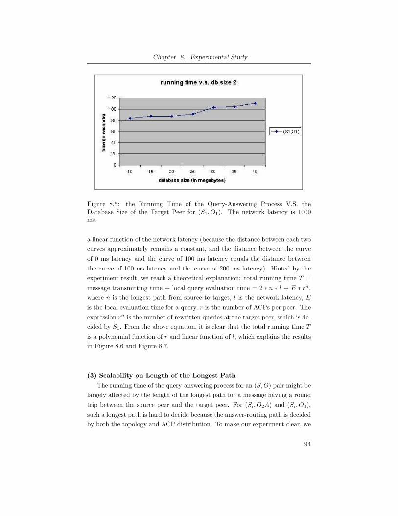
Chapter 8. Experimental Study
Figure 8.5: the Running Time of the Query-Answering Process V.S. theDatabase Size of the Target Peer for (S1, O1). The network latency is 1000ms.
a linear function of the network latency (because the distance between each two
curves approximately remains a constant, and the distance between the curve
of 0 ms latency and the curve of 100 ms latency equals the distance between
the curve of 100 ms latency and the curve of 200 ms latency). Hinted by the
experiment result, we reach a theoretical explanation: total running time T =
message transmitting time + local query evaluation time = 2 ∗ n ∗ l + E ∗ rn,
where n is the longest path from source to target, l is the network latency, E
is the local evaluation time for a query, r is the number of ACPs per peer. The
expression rn is the number of rewritten queries at the target peer, which is de-
cided by S1. From the above equation, it is clear that the total running time T
is a polynomial function of r and linear function of l, which explains the results
in Figure 8.6 and Figure 8.7.
(3) Scalability on Length of the Longest Path
The running time of the query-answering process for an (S, O) pair might be
largely affected by the length of the longest path for a message having a round
trip between the source peer and the target peer. For (Si, O2A) and (Si, O3),
such a longest path is hard to decide because the answer-routing path is decided
by both the topology and ACP distribution. To make our experiment clear, we
94
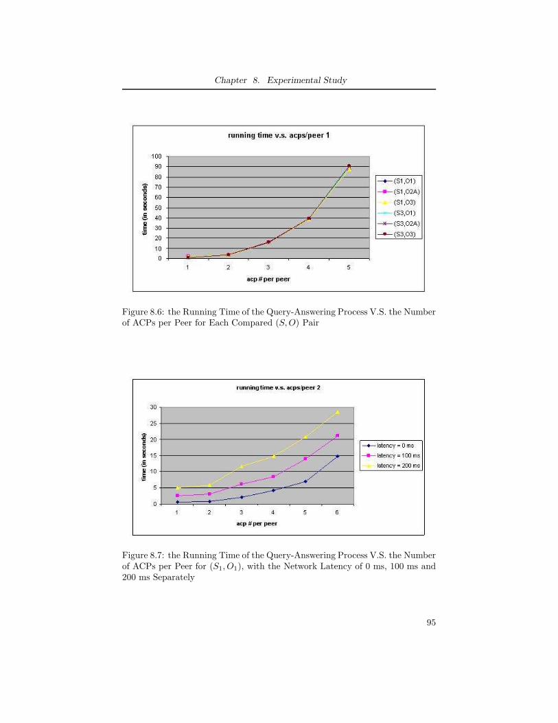
Chapter 8. Experimental Study
Figure 8.6: the Running Time of the Query-Answering Process V.S. the Numberof ACPs per Peer for Each Compared (S, O) Pair
Figure 8.7: the Running Time of the Query-Answering Process V.S. the Numberof ACPs per Peer for (S1, O1), with the Network Latency of 0 ms, 100 ms and200 ms Separately
95
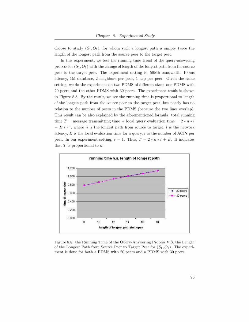
Chapter 8. Experimental Study
choose to study (S1, O1), for whom such a longest path is simply twice the
length of the longest path from the source peer to the target peer.
In this experiment, we test the running time trend of the query-answering
process for (S1, O1) with the change of length of the longest path from the source
peer to the target peer. The experiment setting is: 50Mb bandwidth, 100ms
latency, 1M database, 2 neighbors per peer, 1 acp per peer. Given the same
setting, we do the experiment on two PDMS of different sizes: one PDMS with
20 peers and the other PDMS with 30 peers. The experiment result is shown
in Figure 8.8. By the result, we see the running time is proportional to length
of the longest path from the source peer to the target peer, but nearly has no
relation to the number of peers in the PDMS (because the two lines overlap).
This result can be also explained by the aforementioned formula: total running
time T = message transmitting time + local query evaluation time = 2 ∗ n ∗ l
+ E ∗ rn, where n is the longest path from source to target, l is the network
latency, E is the local evaluation time for a query, r is the number of ACPs per
peer. In our experiment setting, r = 1. Thus, T = 2 ∗ n ∗ l + E. It indicates
that T is proportional to n.
Figure 8.8: the Running Time of the Query-Answering Process V.S. the Lengthof the Longest Path from Source Peer to Target Peer for (S1, O1). The experi-ment is done for both a PDMS with 20 peers and a PDMS with 30 peers.
96
Chapter 9
Conclusions and Future
Work
In this thesis, we have studied the access control issue in the XML peer data
management system. To the best of our knowledge, our work is the first attempt
to systematically analyze the access control problems in the PDMS. Our main
contributions include:
• A formal syntax for the Access Control Policy (ACP) is proposed. The
ACP syntax is fine-grained and expressive enough for specifying the access
control privilege on the XML database of a peer in the PDMS. (Chapter
3)
• We design several (query transmitting) Strategies and (answer routing)
Options, whose combinations form the query-answering algorithms and
can handle the access control requirements in a PMDS. (Chapter 4)
• Some novel algorithms used in the strategies and options, such as (i) query
rewriting algorithm in light of ACPs (ii) safe peer list finding algorithm
(iii) annotating and partitioning algorithm, are designed. (Chapter 7)
• We formalize the definitions for Information Leakage Free and Complete-
ness, which are important properties of an (Strategy, Option) pair. Fur-
thermore, we propose the sufficient and necessary conditions for them, and
analyze every (Strategy, Option) pair designed. (Chapter 5)
• We propose a cost model, which consists of the major tasks and the cor-
responding primitive operations and cost units. All (Strategy, Option)
pairs are assessed by this cost model. (Chapter 6)
• Experiments are conducted on the designed (Strategy, Option) pairs, com-
paring their execution speed and testing the scalability in terms of the tar-
97
Chapter 9. Conclusions and Future Work
get peer database size, ACP amount pe peer, length of the longest path
from the source peer to the target peer. (Chapter 8)
There are some directions that we would like to pursue in our future work:
• In our work we assume that all peers use the same schema, which avoids
adding in the complications of schema heterogeneity. In a realistic PDMS,
the schema heterogeneity will force ACPs to be rewritten if they are dis-
tributed among the PDMS. And the schema heterogeneity may also affect
the query-rewriting in light of ACPs algorithm.
• Caching is not discussed in the thesis. However, as a common approach to
accelerate the query-answering process, caching is worth noting. If caching
is used in a PDMS, we need to be more careful to avoid information
leakage. The IL-free and Completeness definitions in the thesis need to
be modified. And other strategies and options can be designed to utilize
caching.
• Thus far, our algorithm for query-rewriting in light of ACPs can only
handle one fragment of tree patterns, whose corresponding XPath is with
‘/’, ‘//’, ‘[ ]’. And it also requires that nodes of TP R ext have distinct
tags. We would like to remove the restrictions and make the algorithm to
handle more general cases.
98
Bibliography
[1] XMark An XML Benchmark Project, 2003. http://monetdb.cwi.nl/xml/.
[2] Emulab - Network Emulation Testbed, 2006. http://www.emulab.net/.
[3] Pastry: A substrate for peer-to-peer applications, 2006.
http://www.freepastry.org/.
[4] Qizx/open, 2006. http://www.axyana.com/qizxopen/.
[5] S. Adali, K. Candan, Y. Papakonstantinou, and V. Subrahmanian. Query
Caching and Optimization in Distributed Mediator Systems. In Proc. of the
ACM SIGMOD International Conference on Management of Data, 1996.
[6] A. V. Aho, Y. Sagiv, and J. D. Ullman. Efficient Optimization of a Class of
Relational Expressions. ACM Transactions on Database Systems (TODS),
4(4):435–454, 1979.
[7] A. V. Aho, Y. Sagiv, and J. D. Ullman. Equivalence of relational expres-
sions. SIAM Journal on Computing, 8(2):218–246, 1979.
[8] J. L. Ambite, N. Ashish, G. Barish, C. A. Knoblock, S. Minton, P. J.
Modi, I. Muslea, A. Philpot, and S. Tejada. ARIADNE: A System for
Constructing Mediators for Internet Sources (system demonstration). In
Proc. of the ACM SIGMOD International Conference on Management of
Data, 1998.
[9] Sihem Amer-Yahia, SungRan Cho, Laks V. S. Lakshmanan, and Divesh Sri-
vastava. Tree Pattern Query Minimization. The VLDB Journal, 11(4):315–
331, 2002.
[10] Elisa Bertino, Barbara Carminati, and Elena Ferrari. A Temporal Key
Management Scheme for Secure Broadcasting of XML Documents. In Proc.
of the 9th ACM Conference on Computer and Communications Security
(CCS 2002), 2002.
99
Chapter 9. Conclusions and Future Work
[11] J. Biskup, P. Dublish, and Y. Sagiv. Optimization of a subclass of con-
junctive queries. Acta Informatica, 32(1):1–26, 1995.
[12] Scott Boag, Don Chamberlin, Mary F. Fernandez, Daniela Florescu,
Jonathan Robie, and Jerome Simeon. XQuery 1.0: An XML Query Lan-
guage, 2006. http://www.w3.org/TR/xquery/.
[13] Angela Bonifati, Elaine Qing Chang, Laks V.S. Lakshmanan, Terence Ho,
and Rachel Pottinger. HePToX: Marrying XML and Heterogeneity in Your
P2P Databases. In Proc. of the 31st International Conference on Very Large
Databases (VLDB 2005), 2005.
[14] Sabrina De Capitani, Stefania Marrara, and Pierangela Samarati. An Ac-
cess Control Model for Querying XML Data. In Proc. of the 2005 Workshop
on Secure Web Services (SWS 2005), 2005.
[15] Ashok K. Chandra and Philip M. Merlin. Optimal Implementation of Con-
junctive Queries in Relational Data Bases. In Proc. of the 9th annual ACM
Symposium on Theory of Computing (STOC 1977), 1977.
[16] Sudarshan Chawathe, Hector Garcia-Molina, Joachim Hammer, Kelly Ire-
land, Yannis Papakonstantinou, Jeffrey Ullman, and Jennifer Widom.
The TSIMMIS Project: Integration of Heterogeneous Information Sources.
Journal of Intelligent Information Systems, 8(2):117–132, 1997.
[17] Chandra Chekuri and Anand Rajaraman. Conjunctive Query Containment
Revisited. Theoretical Computer Science, 239(2):211–229, 1998.
[18] ERNESTO DAMIANI. A Fine-Grained Access Control System for XML
Documents. ACM Transactions on Information and System Security,
5(2):169–202, 2002.
[19] Xin Dong, Alon Y. Halevy, and Igor Tatarinov. Containment of Nested
XML Queries. In Proc. of the 30th International Conference on Very Large
Databases (VLDB 2004), 2004.
[20] S. Flesca, F. Furfaro, and E. Masciari. On the minimization of Xpath
queries. In Proc. of the 29th International Conference on Very Large
Databases (VLDB 2003), 2003.
[21] Alban Gabillon. A Formal Access Control Model for XML Databases. In
Proc. of the VLDB Workshop on Secure Data Management (SDM), 2005.
100
Chapter 9. Conclusions and Future Work
[22] L. Haas, D. Kossmann, E. Wimmers, and J. Yang. Optimizing Queries
across Diverse Data Sources. In Proc. of the 23rd International Conference
on Very Large Databases (VLDB 1997), 1997.
[23] Alon Y. Halevy, Zachary G. Ives, Jayant Madhavan, Peter Mork, Dan
Suciu, and Igor Tatarinov. The Piazza Peer Data Management System.
IEEE Transactions on Knowledge and Data Engineering, 2004.
[24] Alon Y. Halevy, Zachary G. Ives, Peter Mork, and Igor Tatarinov. Piazza:
Data Management Infrastructure for Semantic Web Applications. In Proc.
of the 12th International World Wide Web Conference (WWW2003), 2003.
[25] C. Ilioudis, G. Pangalos, and A. Vakali. Security model for XML data.
In Proc. of the 2nd International Conference on Internet Computing (IC
2001), 2001.
[26] D.S. Johnson and A.Klug. Optimizing Conjunctive Queries that Contain
Untyped Variables. SIAM Journal on Computing, 12(4):616–640, 1983.
[27] Phokion G. Kolaitis and Moshe Y. Vardi. Conjunctive-Query Contain-
ment and Constraint Satisfaction. In Proc. of the 17th ACM SIGMOD-
SIGACT-SIGART Symposium on Principles of Database Systems (PODS
1998), 1998.
[28] E. Lambrecht, S. Kambhampati, and S. Gnanaprakasam. Optimizing Re-
cursive Information Gathering Plans. In Proc. of the 16th International
Joint Conference on Artificial Intelligence, 1999.
[29] Maurizio Lenzerini. Data Integration: A Theoretical Perspective. In Proc.
of the 21st ACM SIGMOD-SIGACT-SIGART Symposium on Principles of
Database Systems (PODS 2002), 2002.
[30] A. Y. Levy, A. Rajaraman, and J. J. Ordille. Querying Heterogeneous
Information Sources Using Source Descriptions. In Proc. of the 22nd In-
ternational Conference on Very Large Databases (VLDB 1996), 1996.
[31] I. Manolescu, D. Florescu, , and D. Kossmann. Answering XML Queries
over Heterogeneous Data Sources. In Proc. of the 27th International Con-
ference on Very Large Databases (VLDB 2001), 2001.
[32] Gerome Miklau. Research Problems in Secure Data Exchange. Technical
report, University of Washington, March 2004.
101
Chapter 9. Conclusions and Future Work
[33] Gerome Miklau and Dan Suciu. Containment and Equivalence for an XPath
Fragment. In Proc. of the 21st ACM SIGMOD-SIGACT-SIGART Sympo-
sium on Principles of Database Systems (PODS 2002), 2002.
[34] Gerome Miklau and Dan Suciu. Containment and Equivalence for a Frag-
ment of XPath. Journal of the ACM (JACM), 51(1):2–45, 2004.
[35] Wee Siong Ng, Beng Chin Ooi, Kian-Lee Tan, and Aoying Zhou. PeerDB:
A P2P-based System for Distributed Data Sharing. In Proc. of the 19th
International Conference on Data Engineering (ICDE 2003), 2003.
[36] Prakash Ramanan. Efficient Algorithms for Minimizing Tree Pattern
Queries. In Proc. of the ACM SIGMOD International Conference on Man-
agement of Data, 2002.
[37] Patricia Rodrguez-Gianolli, Maddalena Garzetti, Lei Jiang, Anastasios Ke-
mentsietsidis, Iluju Kiringa, Mehedi Masud, Rene J. Miller, and John My-
lopoulos. Data Sharing in the Hyperion Peer Database System. In Proc. of
the 31st International Conference on Very Large Databases (VLDB 2005),
2005.
[38] Thomas Schwentick. XPath Query Containment. SIGMOD Record,
33(1):101–109, 2004.
[39] OASIS Standard. eXtensible Access Control Markup Language (XACML)
Version 1.0, 2003. http://www.oasis-open.org/committees/xacml/.
[40] Igor Tatarinov, Zachary Ives, Jayant Madhavan, Alon Halevy, Dan Suciu,
Nilesh Dalvi, Xin (Luna) Dong, Yana Kadiyska, Gerome Miklau, and Peter
Mork. The Piazza Peer Data Management Project. SIGMOD Record,
32(3):47–52, 2003.
[41] Jeffrey D. Ullman. Principles of Database and Knowlege-Based Systems.
Computer Science Press, 1989.
[42] Peter T. Wood. Minimising Simple XPath Expressions. In Proc. of the 4th
International Workshop on the Web and Databases (WebDB 2001), 2001.
[43] M. Yannakakis. Algorithms for Acyclic Database Schemes. In Proc. of
the 7th International Conference on Very Large Databases (VLDB 1981),
1981.
102


![Current Trends in Information Searching/Query Answering€¦ · Current Trends in Information Searching/Query Answering ... database systems developed at Berkeley. ... [Lennox Berkeley]](https://img.dokumen.tips/doc/110x75/5b4ac5b27f8b9a691e8c6434/current-trends-in-information-searchingquery-answering-current-trends-in-information.jpg)