Accelerating Successive Approximation Algorithm … Tandem Queueing System ... successive approximation, policy iteration, ... Introduction and Thesis Outline 3 2. Successive over

Accelerating Successive Approximation Algorithm viaAction Elimination

by

Nasser Mohammad Ahmad Jaber

A thesis submitted in conformity with the requirementsfor the degree of Doctor of Philosophy

Graduate Department of Mechanical and Industrial EngineeringUniversity of Toronto

Copyright c© 2008 by Nasser Mohammad Ahmad Jaber

Abstract

Accelerating Successive Approximation Algorithm via Action Elimination

Nasser Mohammad Ahmad Jaber

Doctor of Philosophy

Graduate Department of Mechanical and Industrial Engineering

University of Toronto

2008

This research is an effort to improve the performance of successive approximation algo-

rithm with a prime aim of solving finite states and actions, infinite horizon, stationary,

discrete and discounted Markov Decision Processes (MDPs). Successive approximation

is a simple and commonly used method to solve MDPs. Successive approximation often

appears to be intractable for solving large scale MDPs due to its computational complex-

ity. Action elimination, one of the techniques used to accelerate solving MDPs, reduces

the problem size through identifying and eliminating sub-optimal actions. In some cases

successive approximation is terminated when all actions but one per state are eliminated.

The bounds on value functions are the key element in action elimination. New terms

(action gain, action relative gain and action cumulative relative gain) were introduced

to construct tighter bounds on the value functions and to propose an improved action

elimination algorithm.

When span semi-norm is used, we show numerically that the actual convergence of

successive approximation is faster than the known theoretical rate. The absence of easy-

to-compute bounds on the actual convergence rate motivated the current research to try

a heuristic action elimination algorithm. The heuristic utilizes an estimated convergence

rate in the span semi-norm to speed up action elimination. The algorithm demonstrated

exceptional performance in terms of solution optimality and savings in computational

time.

ii

Certain types of structured Markov processes are known to have monotone optimal

policy. Two special action elimination algorithms are proposed in this research to accel-

erate successive approximation for these types of MDPs. The first algorithm uses the

state space partitioning and prioritize iterate values updating in a way that maximizes

temporary elimination of sub-optimal actions based on the policy monotonicity. The

second algorithm is an improved version that includes permanent action elimination to

improve the performance of the algorithm. The performance of the proposed algorithms

are assessed and compared to that of other algorithms. The proposed algorithms demon-

strated outstanding performance in terms of number of iterations and computational time

to converge.

iii

Dedication

To my parents, sister & brothers, and my beloved wife & sons

iv

Acknowledgements

I would like to express my sincere gratitude to my supervisor Professor Chi-Guhn Lee

for his guidance, suggestions and endless patience and support during my research work.

I also thank my thesis supervisory and examination committee, namely, Professors Viliam

Makis, Roy Kwon, Baris Balcioglu and Daniel Frances for their constructive feedback.

I am grateful to The Hashemite University and The University of Toronto for provid-

ing me with the financial support needed to complete my Ph.D. study.

Thanks are extended to my friends Mohammad Alameddine, Mohammad Ahmad,

Mahdi Tajbakhsh, Wahab Ismail, Zhong Ma, Jun Liu and Kevin Ferreira for the friendly

environment and wonderful days we shared together during my study.

Last and foremost, I am deeply grateful to my beloved wife for her continuous en-

couragement and support through my study. I am indebted to my parents, sister and

brothers for their endless care and love

v

Contents

1 Introduction and Thesis Outline 1

1.1 Introduction . . . . . . . . . . . . . . . . . . . . . . . . . . . . . . . . . . 1

1.2 Motivations . . . . . . . . . . . . . . . . . . . . . . . . . . . . . . . . . . 3

1.3 Objectives . . . . . . . . . . . . . . . . . . . . . . . . . . . . . . . . . . . 5

1.4 Methodology . . . . . . . . . . . . . . . . . . . . . . . . . . . . . . . . . 6

1.5 Thesis Outline . . . . . . . . . . . . . . . . . . . . . . . . . . . . . . . . . 8

2 Markov Decision Processes 10

2.1 Introduction . . . . . . . . . . . . . . . . . . . . . . . . . . . . . . . . . . 10

2.2 Successive Approximation . . . . . . . . . . . . . . . . . . . . . . . . . . 11

2.3 Policy Iteration . . . . . . . . . . . . . . . . . . . . . . . . . . . . . . . . 14

2.4 Linear Programming . . . . . . . . . . . . . . . . . . . . . . . . . . . . . 16

2.5 Accelerated Algorithms . . . . . . . . . . . . . . . . . . . . . . . . . . . . 17

2.5.1 Value Iteration Schemes . . . . . . . . . . . . . . . . . . . . . . . 18

2.5.2 Relaxation Approaches . . . . . . . . . . . . . . . . . . . . . . . . 18

2.5.3 Hybrid Approaches . . . . . . . . . . . . . . . . . . . . . . . . . . 19

2.5.4 General Approaches . . . . . . . . . . . . . . . . . . . . . . . . . 20

2.6 Literature Review . . . . . . . . . . . . . . . . . . . . . . . . . . . . . . . 20

3 Improved Action Elimination 25

3.1 Action Elimination . . . . . . . . . . . . . . . . . . . . . . . . . . . . . . 25

vi

3.2 Norms and VI Schemes Performance . . . . . . . . . . . . . . . . . . . . 28

3.3 Action Gain and Action Relative Gain . . . . . . . . . . . . . . . . . . . 29

3.4 Improved Action Elimination Algorithm . . . . . . . . . . . . . . . . . . 31

3.5 Numerical Studies . . . . . . . . . . . . . . . . . . . . . . . . . . . . . . . 35

3.6 Conclusion . . . . . . . . . . . . . . . . . . . . . . . . . . . . . . . . . . . 45

4 Heuristic Action Elimination 46

4.1 Theoretical and Actual Convergence Rates . . . . . . . . . . . . . . . . . 47

4.2 Estimated Convergence Rate . . . . . . . . . . . . . . . . . . . . . . . . . 50

4.3 Heuristic Action Elimination Algorithm . . . . . . . . . . . . . . . . . . . 50


4.5 Conclusion . . . . . . . . . . . . . . . . . . . . . . . . . . . . . . . . . . . 56

5 Action Elimination for Monotone Policy MDPs 57

5.1 Monotone Policy MDPs . . . . . . . . . . . . . . . . . . . . . . . . . . . 57

5.2 Action Elimination for MPMDPs . . . . . . . . . . . . . . . . . . . . . . 59


5.3.1 Case Study . . . . . . . . . . . . . . . . . . . . . . . . . . . . . . 71

5.3.2 Numerical Studies Results . . . . . . . . . . . . . . . . . . . . . . 73

5.4 Conclusion . . . . . . . . . . . . . . . . . . . . . . . . . . . . . . . . . . . 77

6 Conclusions and Future Research 80

6.1 Conclusions . . . . . . . . . . . . . . . . . . . . . . . . . . . . . . . . . . 80

6.2 Contributions . . . . . . . . . . . . . . . . . . . . . . . . . . . . . . . . . 83

6.3 Future Research . . . . . . . . . . . . . . . . . . . . . . . . . . . . . . . . 84

A Numerical Study Results 86

Bibliography 99

vii

List of Tables

3.1 Abbreviations used in numerical studies . . . . . . . . . . . . . . . . . . 36

3.2 Average values for γ . . . . . . . . . . . . . . . . . . . . . . . . . . . . . 40

3.3 Performance of PAE and HAE1 in AN and AT (|S|=100) . . . . . . . . . 41

4.1 Average values for λmax, αmax, γ and the ratio αmax/λγ . . . . . . . . . 49

4.2 comparison of αIn and αIIn . . . . . . . . . . . . . . . . . . . . . . . . . . 51

4.3 Performance evaluation of HAE compared to PAE (|S|=200) . . . . . . . 54

5.1 The sequencing and the search range for the minimizers of the states in

{Ss} . . . . . . . . . . . . . . . . . . . . . . . . . . . . . . . . . . . . . . 62

5.2 Performance results summary (AN) . . . . . . . . . . . . . . . . . . . . . 74

5.3 Performance results summary (AT) . . . . . . . . . . . . . . . . . . . . . 75

A.1 Performance evaluation for PJVI (|S|=100) . . . . . . . . . . . . . . . . . 87

A.2 Performance evaluation for JVI (|S|=100) . . . . . . . . . . . . . . . . . . 88

A.3 Performance evaluation for PGSVI (|S|=100) . . . . . . . . . . . . . . . . 89

A.4 Performance evaluation for GSVI (|S|=100) . . . . . . . . . . . . . . . . 90

A.5 Performance evaluation for PAE and HAE1 (AN and AT)(|S|=100) . . . 91

A.6 Performance evaluation for PAE, HAE2 and IAE (AN) (|S|=200) . . . . 92

A.7 Performance evaluation for PAE, HAE2 and IAE (AT) (|S|=200) . . . . 93

A.8 Performance evaluation for PAE and HAE (AN and AT)(|S|=200) . . . . 94

A.9 Performance evaluation for PJVI, HTAE and MPAE1 (AN) (|S|=35937) 95

viii

A.10 Performance evaluation for PAE, P+HTAE and MPAE2 (AN) (|S|=35937) 96

A.11 Performance evaluation for PJVI, HTAE and MPAE1 (AT ) (|S|=35937) 97

A.12 Performance evaluation for PAE, P+HTAE and MPAE2 (AT ) (|S|=35937) 98

ix

List of Figures

3.1 Flow chart diagram for the IAE algorithm . . . . . . . . . . . . . . . . . 33

3.2 VI schemes performance in AN (λ = 0.80) . . . . . . . . . . . . . . . . . 37

3.3 VI schemes performance in AN (λ = 0.99) . . . . . . . . . . . . . . . . . 38

3.4 VI schemes performance in AT (λ = 0.80) . . . . . . . . . . . . . . . . . 38

3.5 VI schemes performance in AT (λ = 0.99) . . . . . . . . . . . . . . . . . 39

3.6 Performance of PAE and HAE1 in AN (|S| = 100) . . . . . . . . . . . . . 42

3.7 Performance of PAE and HAE1 in AT (|S| = 100) . . . . . . . . . . . . . 43

3.8 Performance of PAE, HAE2 and IAE in AN (|S| = 200) . . . . . . . . . . 44

3.9 Performance of PAE, HAE2 and IAE in AT (|S| = 200) . . . . . . . . . . 44

4.1 Performance of P-AE and H-AE (AN vis TPMS) . . . . . . . . . . . . . 55

4.2 Performance of P-AE and H-AE (AT vis TPMS) . . . . . . . . . . . . . . 55

5.1 Temporary action elimination utilizing monotonicity (1) . . . . . . . . . . 63



5.4 Tandem Queueing System (three queues in series) . . . . . . . . . . . . . 72

5.5 The influence of the parameter b on MPAE1 and MPAE2 (λ = 0.90) . . 76

5.6 The influence of the parameter b on MPAE1 and MPAE2 (λ = 0.97) . . 77

5.7 Performance comparison (AT vis AAPS) (λ = 0.90) . . . . . . . . . . . . 78

5.8 Performance comparison (AT vis AAPS) (λ = 0.97) . . . . . . . . . . . . 78

x

Chapter 1

Introduction and Thesis Outline

1.1 Introduction

Markov chains were introduced by the Russian mathematician A. A. Markov in early

20th century (Puterman, 1994) . Later Markov decision processes (MDPs) were devel-

oped and became an elegant framework for modeling stochastic dynamic programming.

During the last fifty years, huge efforts have been dedicated to investigate and discover

more applications that can be modeled as MDPs. Some of the MDPs applications to

be mentioned are Queueing Systems (Serfozo, 1981; Lu and Serfozo, 1984; Weber,

1987; Yannopoulos and Alfa, 1993 and Chen and Meyn, 1999), Production Planning

(Presman et al., 1995; 2001; Sethi et al., 2000; Haskose et al, 2002 and 2004), Inven-

tory Control (Adachi et al., 1999; Demchenko et al., 2000; Ohno and Ishigaki, 2001;

Fleischmann and Kuik, 2003 and Benjaafar and Elhafsi, 2006), and Maintenance Man-

agement (Derman, 1963; Anderson, 1994; Lam, 1997; Moustafa et al., 2004; Chan et

al., 2006 and Tamura, 2007).

This research will focus on the MDPs as a special methodology for the sequential

decision making, which has been and will continue to be one of the most challenging

research subjects in the area of operations research. Different types of MDPs have been

1

Chapter 1. Introduction and Thesis Outline 2

discussed and analyzed in the literature (White and White, 1989 and Puterman, 1994).

MDPs are classified as stationary (homogeneous) if the transition probabilities, the one

step rewards or costs, and the set of admissible actions for each state do not vary with

time. If any of the previously mentioned elements is a function of time, then the MDP

is classified as non-stationary. The states, the actions and the planning horizon can be

either finite or infinite. The optimization criterion is to maximize (minimize) the expected

total discounted or the expected average long run rewards (costs). If the system under

control is monitored all the time and the actions are taken at the appropriate instance,

then the MDP is said to be continuous; otherwise, it is classified as discrete (Puterman,

1994).

This research is concerned with stationary, finite states and actions, infinite hori-

zon, discrete and discounted MDPs. MDPs of this type are usually solved using one of

three methods: successive approximation, policy iteration, and linear programming. An

overview of these methods will be presented in Chapter 2.

Although MDPs provides a powerful and compact way of modeling complex deci-

sion making problems, its high computational complexity, better known as 88curse of

dimensionality′′, limits its applicability to many practical problems (Puterman, 1994;

Littman et al., 1998; Littman et al., 2000 and de Farias and Roy, 2004). Researchers

have investigated different approaches to solve MDPs faster. Previous research in this

field pursued two main directions; the first worked on accelerating the convergence to the

optimal or ε-optimal solutions while the other sought out approximate solutions.

In their effort to speeds up solving the MDPs, researchers have tried different methods

that can be further classified into four main groups:

1. Improved versions of the recursive equations known as Successive Approximation or

Value Iteration (VI) schemes, namely: Pre-Jacobi VI (PJVI), Jacobi VI (JVI), Pre-

Gauss-Seidel VI (PGSVI), and Gauss-Seidel VI (GSVI) (Blackwelli, 1965; Kushner,

1971; Porteus, 1975; 1978; 1981 and Thomas et al., 1983).


2. Successive over relaxation and extrapolation (Popyack et al., 1979; Thomas et al.,

1983; Herzberg, 1991; 1994 and 1996).

3. Hybrid algorithms where two or more different algorithms are combined to come

up with a new algorithm (Puterman and Shin, 1978; Dembo and Haviv, 1984 and

Herzberg, 1996).

4. General techniques that can accelerate most of the algorithms used to solve MDPs:

Action Elimination (MacQeens, 1967; Porteus, 1971; Hastings and Mello, 1973;

Hubner, 1977; 1980; Koehler, 1981 and Puterman and Shin, 1982), Decomposi-

tion (Ruszczynski, 1997; Madras and Randall, 2002; Abbad and Boustique, 2003

and Umanita, 2006) and State Space Partitioning (Wingate and Seppi, 2003;

Kim and Dean, 2003; Lee and Lau, 2004 and Jin et al., 2007).

In the second direction, researchers have tried different ways to approximate the opti-

mal solution. Aggregation and Disaggregation in the state space were implemented

to find approximate solutions (Haviv, 1987; 1999; Buchholz, 1999; Marek, 2003a and

Marek and Mayer, 2003b). Basis Functions were used to approximate the decision

variables (the value functions) in linear programming models (Schweitzer and Seidmann,

1985; Trick and Zin, 1993; 1997 and de Farias and Roy, 2004).

1.2 Motivations

MDPs provide a framework for modeling stochastic dynamic programming with a broad

range of applications. Despite the advanced computational capabilities in terms of both

machines and software solvers, solving large scale MDPs exactly within reasonable time,

is still a great challenge. Action Elimination (AE) was introduced by MacQueen (1967)

to accelerate successive approximation algorithm when solving discrete and discounted

MDPs. Porteus (1971) introduced new bounds for discounted sequential decision pro-


cesses and suggested AE test similar to MacQueen’s AE test. Hubner (1977) improved

the bound on the convergence rate utilizing delta coefficient (δ) which provides an upper

bound on the sub-radius (modulus of the second largest eigenvalue) of the transition

probability matrix (TPM) (Puterman, 1994). Hubner’s work was the last effort to im-

prove AE for general discounted MDPs. Later, a few AE algorithms were suggested to

accelerate solving special types of MDPs which are not related to this research (Even-Dar

et al., 2006; Kuter and Hu, 2007 and Novoa, 2007).

Based on literature review carried out during this research, the performance of Hub-

ner’s AE algorithm was not tested or compared to other algorithms. Hubner (1977)

assessed the value of δ for some problems discussed in the literature and stated his con-

cerns regarding the effort needed to calculate δ. He suggested using weaker bound (δ′)

which is easier to be calculated than δ . Zobel and Scherer (2005) discussed the ef-

fectiveness of δ and δ′ and they underlined that most likely δ′ = 1 when the TPM is

sparse.

As part of this research, Hubner’s AE algorithm is assessed in comparison to Porteus’

AE algorithm and we found that there is a room for improvement. That is, the current

research is to improve Hubner’s AE algorithm to overcome some of its drawbacks as will

be presented in Chapter 3.

The convergence rate is a key factor in AE where smaller convergence rate provides

tighter bounds and as a result more efficient AE. The convergence rate in the first few

iterations of the successive approximation algorithm is known to be faster than the long

run rate in the supremum norm (sup-norm) (White and Scherer, 1994 and Puterman,

1994). We conducted numerical studies to assess the actual convergence in both sup-

norm and span semi-norm. Motivated by the numerical results in the span semi-norm,

a simple and effective heuristic AE algorithm was suggested and tested as presented in

Chapter 4.


Certain type of structured MDPs, monotone policy MDPs (MPMDPs), are very com-

mon in may applications. Heyman and Sobel (1984) suggested a special successive ap-

proximation algorithm that utilizes the policy monotonicity to eliminate, temporarily,

sub-optimal actions when solving MPMDPs. State space partitioning (Wingate and

Seppi, 2003; Kim and Dean, 2003; Lee and Lau, 2004 and Jin et al., 2007) and states pri-

oritization (Wingate and Seppi, 2005) were used separately to accelerate solving MDPs

in general. This research employed the state space partitioning and prioritize states to be

updated in a way that maximizes temporarily elimination of sub-optimal actions based

on policy monotonicity. Two special AE algorithms are proposed to speedup successive

approximation algorithm when solving MPMDPs. This will be discussed in more details

in Chapter 5.

1.3 Objectives

The prime objective of this research is to improve the performance of the successive

approximation algorithm using AE in solving specific type of MDPs, explicitly the discrete

and discounted, finite states and actions, infinite horizon, and stationary. The following

sub-objectives are set to achieve the prime objective:

Sub-Objective 1 Improve Hubner’s AE algorithm.

Sub-Objective 2 Propose a heuristic algorithm to improve AE and speedup the suc-

cessive approximation algorithm.

Sub-Objective 3 Introduce a special AE algorithm for monotone policy MDPs.


1.4 Methodology

Four different successive approximation schemes (PJVI, JVI, PGSVI and GSVI) and

two stopping criteria (sup-norm and span semi-norm) were discussed in the literature.

The performance of the four schemes was assessed in the sup-norm (Kushner, 1971 and

Thomas et al., 1983), while no performance evaluation has been done with the span semi-

norm. In this research, the performance of the four schemes in both sup-norm and span

semi-norm will be assessed using randomly generated MDPs. The performance measures

will include the number of iterations and the computational time (CPUT) to converge.

This assessment aims at selection of the best performing scheme and norm to be the

successive approximation platform through out this research.

In order to achieve the prime and sub-objectives of this research, the following method-

ology will be developed based on observations through reviewing the literature.

1. To improve the performance of Hubner’s AE algorithm. The literature of AE is

studied and is found to have a room for improvement. New terms are introduced

to drive tighter bounds on the value functions. These bounds are used to improve

Hubner’s AE test. An assessment for the performance of Hubner’s AE algorithm

is conducted in comparison to Porteus’ AE algorithm utilizing randomly generated

problems. The comparison aimed to prevail any hidden drawbacks in Hubner’s al-

gorithm, which will be considered in the development of an improved AE algorithm

to be proposed. Then the proposed algorithm is tested, its performance is compared

to that of Porteus and Hubner using randomly generated MDPs, the comparison

criteria are the number of iterations and CPUT to converge.

2. The convergence rate is a key factor in the action elimination technique. The

known theoretically proved bounds on the convergence rates in sup-norm and span

semi-norm are very harsh especially when the discounted factor is very close to

1. To achieve the second sub-objective through better understanding of the actual


convergence behavior; a numerical studies to assess the actual convergence ratios

of the standard successive approximation (PJVI) algorithm is conducted in both

sup-norm and span semi-norm using randomly generated MDPs. The numerical

results are analyzed to suggest an estimator for the actual convergence rate which

is used to propose heuristic AE algorithm. The proposed AE heuristic utilize the

estimated actual convergence rate to replace the upper bound on the convergence

rate in Porteus’ AE algorithm. The performance of the proposed heuristic is tested

in terms of the optimality of the solution and savings in number of iterations and

CPUT compared to Porteus AE algorithm.

3. To achieve the third sub-objective, two special designed action elimination algo-

rithm that maximizes the temporary action elimination based on policy mono-

tonicity suggested by Heyman and Sobal (1984) is developed utilizing the state

space partitioning and priority rule for selecting the state to be updated. The first

algorithm is a modification of the PJVI algorithm to include state space partition-

ing, priority rule for the states to be updated, and more restrictions on the search

range of the best action for each state. The second algorithm is an improved ver-

sion of the first proposed algorithm that includes permanent AE test. The first

algorithm terminates successfully based on span semi-norm stopping criterion only,

while it is possible for the second algorithm to be terminated due to AE. For the

second algorithm, some verified rules that are used to eliminate sub-optimal ac-

tions permanently based on monotonicity are stated, the optimality of the solution

is confirmed in case that termination is based on AE. The performance of the two

proposed algorithms is assessed and compared to the performance of relevant al-

gorithms in terms of number of iterations and CPUT to converge using randomly

generated MPMDPs.


All numerical studies conducted in this research employed special codes that were

developed by the researcher using C++. The numerical results are presented at the end

of each chapter.

1.5 Thesis Outline

This thesis is organized in six chapters. Chapter 2 briefly introduces MDPs, basic defini-

tions and models formulation, the most common algorithms used to solve MDPs namely:

successive approximation, policy iteration and linear programming. The most common

techniques used to accelerate solving MDPs and literature review of relevant research

work. Chapter 3 provides basic concepts used to improve Hubner’s action elimination

algorithm, the suggested algorithm is described, the results are presented and discussed.

In Chapter 4, theoretical and actual convergence rates in sup-norm and span semi-norm

are defined, an estimated convergence rate is used to introduce a heuristic action elimi-

nation algorithm. The new algorithm is tested and the results are discussed. Chapter 5

reviews basic results concerning structured MDPs that have monotone optimal policies,

two special action elimination algorithms are suggested, assessed and compared to other

algorithms. Chapter 6 concludes main findings and provides directions for future research.

A summary of the content of each chapter is presented next.

Chapter 2. Markov Decision Processes

In this chapter an overview of MDPs as a framework to model and solve stochastic

dynamic programming problems is provided. The main classes of the MDPs studied

in the literature are listed and the problem under consideration is defined. Some basic

concepts that are essential to proceed with this work are discussed. The most popular

algorithms used to solve MDPs, namely: successive approximation, policy iteration and

linear programming are discussed. The problem complexity is highlighted, finally, a


literature review is presented.

Chapter 3. Improved Action Elimination

The most relevant action elimination algorithms are discussed. Basic concepts, such as

norms, bounds, action gain and action relative gain that are used to improve Hubner’s

AE algorithm are defined, the improved algorithm is introduced. The performance of the

new algorithm is assessed, and the numerical studies results are presented and discussed.

Chapter 4. Heuristic Action Elimination

Theoretical and actual convergent rates are discussed, an estimation of the actual con-

vergence rate is used to suggest a heuristic action elimination algorithm. A numerical

studies is conducted to test the performance of the suggested heuristic algorithm in terms

of optimality and savings in the computational efforts.

Chapter 5. Action Elimination for Monotone Policy MDPs

A review of basic results for MPMDPs in the literature is provided. Two special designed

action elimination algorithms for MPMDPs are introduced, the optimality of the solution

is verified, the performance of the new algorithms are tested and compared with other

algorithms, and the numerical results are presented and discussed.

Chapter 6. Conclusions and Future Research

The conclusions are stated and directions for future research in action elimination are

suggested.

Chapter 2

Markov Decision Processes

2.1 Introduction

Markov Decision Processes (MDPs) were developed to be a compact and powerful

tool for modeling stochastic dynamic programming and decision making for different ap-

plications: production planning, inventory control, maintenance management, queueing

systems and many other applications. The ultimate goal for any decision maker is to find

an optimal policy, which is a function that tells what action should be selected when the

system is in any of its possible states. Over the last five decades, different types of MDP

problems have been modeled and analyzed. This research is concerned with specific type

of MDPs, which is the stationary, finite states and actions, infinite horizon, discrete and

discounted MDPs. It is well known that for the expected total discounted MDPs with

moderate conditions, there is always a stationary deterministic policy that is optimal

(White and White, 1989 and Puterman, 1994); therefore, the word 88policy′′ will be used

to refer to stationary deterministic policy. The value function for a state i (ν(i)) is a

function that maps state i to its expected total discounted rewards (costs). The following

equations can be used to characterize the optimal value functions and policy (Puterman,

10

Chapter 2. Markov Decision Processes 11

1994).

ν(i) = maxa∈A(i)

{r(i, a) + λ∑j∈S

P (j|i, a)ν(j)}, ∀i ∈ S. (2.1)

where:

• S is a finite set of all possible states of the system

• A is a finite set of all possible actions to be taken at any state of the system

• A(i) is a subset of A containing all the possible actions to be considered when the

system is in state i ∈ S

• P (j\i, a) is a one-step conditional transition probability from state i to state j when

decision a is selected, a ∈ A(i), i, j ∈ S.∑

j∈S P (j\i, a) = 1, ∀ a ∈ A(i), i ∈ S.

• r(i, a) is a bounded one-step reward if action a is selected in state i, |r(i, a)| ≤M <

∞.

• ν(i) ∈ V , V is the partially ordered and normed linear space of bounded value

functions on S

• λ is a discounting factor, 0 ≤ λ < 1

The most common methods used to solve MDPs are successive approximation, policy

iteration, and linear programming. An overview of these methods is presented in the

following sections.

2.2 Successive Approximation

The successive approximation, known as Value Iteration (VI) algorithm, is one of

the most widely used and simplest algorithms for solving MDPs. Standard VI, referred

to as Pre-Jacobi VI (PJVI), is the simplest VI scheme. Consider return maximization

problem, starting at an arbitrary value functions (ν0 ∈ V ), the iterate values (νn) are


calculated using the following recursive equations (Blackwell, 1965; Kushner, 1971 and

Porteus, 1975)

νn(i) = maxa∈A(i)

{r(i, a) + λ∑j∈S

P (j\i, a)νn−1(j)}, ∀ i ∈ S, n = 1, 2, . . . (2.2)

The algorithm terminates successfully in finite number of iterations (N) based on

sup-norm stopping criteria. The algorithm returns an ε-optimal fixed point (ν∗sup) if

‖νN − νN−1‖ < ε(1− λ)/2λ (2.3)

ν∗sup = νN (2.4)

where ε is a predetermined tolerance, and the sup-norm (‖ ‖) is defined as follows

‖ν‖ = maxi∈S{|ν(i)|} (2.5)

utilizing the ν∗sup, an ε-optimal stationary policy that applies the same decision rule

d∗ε is identified as follows:

d∗ε(i) ∈ arg maxa∈A(i){r(i, a) + λ∑j

P (j\i, a)ν∗sup(j)} (2.6)

Detailed description for the standard value iteration (PJVI) algorithm using the sup-norm

stopping criteria is as follows (Puterman, 1994 and Gosavi, 2003):

Step 1 - Initialization: Set ν0 = 0, specify ε > 0 and set n = 1.

Step 2 - Value improvement: For each i ∈ S, compute νn(i)


{r(i, a) + λ∑j∈S

P (j\i, a)νn−1(j)},∀ i ∈ S.

Step 3 - Test for the stopping criterion: If ‖νn− νn−1‖ < ε(1− λ)/2λ go to step 4;

otherwise, increment n by 1 and return to step 2.

Step 4 - ε-Optimal policy identification and termination: For each i ∈ S


1. Set ν∗sup(i) = νn(i)

2. choose d∗ε(i) such that,


P (j\i, a)ν∗sup(j)}.

3. STOP

The sup-norm decreases slowly as the algorithm approaches the fixed point, the con-

vergence is extremely slow when the discounting factor is very close to one (Harzberg

and Yechiali, 1994). The convergence to the point that satisfies the span semi-norm

stopping criteria (νspan) is often much faster than the convergence to the ν∗sup (Puterman,

1994; Gosavi, 2003 and Zobel and scherer, 2005). Adopting the span semi-norm stopping

criteria the algorithm terminates in finite number of iterations (N) when

sp (νN − νN−1) < ε(1− λ)/λ (2.7)

then

νspan = νN (2.8)

where

sp (ν) = maxi∈S{ν(i)} − min

i∈S{ν(i)} (2.9)

The algorithm returns an ε-optimal fixed point (ν∗span). The relation between νspan and

ν∗span is that

ν∗span = νspan + C · e (2.10)

where e is a vector in which all components equal 1 and C is a constant (Puterman,

1994). C is calculated based on maximum and minimum state gain in the last iteration

(∆maxN (i)) and (∆min

N (i)), respectively, where:

∆maxN = max

i∈S{νN(i)− νN−1(i)} (2.11)

∆minN = min

i∈S{νN(i)− νN−1(i)} (2.12)


C = (∆maxn + ∆min

n )/2(1− λ) (2.13)

Gosavi (2003) suggested utilizing the span semi-norm stopping criterion in the standard

value iteration algorithm as follows:

Step 1 - Initialization: Set ν0 = 0, specify ε > 0, set n = 1.

Step 2 - Value improvement: For each i ∈ S, compute νn(i)


{r(i, a) + λ∑j∈S

P (j\i, a)νn−1(j)},∀ i ∈ S.

Step 3 - Test for stopping criterion: If sp(νn − νn−1) < ε(1 − λ)/λ go to step 4;

otherwise, increment n by 1 and return to step 2.

Step 4 - Optimal policy identification and termination: For each i ∈ S

1. Set ν∗span(i) = νn(i) + (∆maxn + ∆min

n )/2(1− λ),



P (j\i, a)ν∗span(j)}.

3. STOP

2.3 Policy Iteration

The second common algorithm used to solve MDPs is the Policy Iteration (PI) algo-

rithm. Bellman (1957) suggested preliminary version of the PI which is named 88approximation

in policy space′′. Howard (1960) introduced the formal algorithm which is known as PI

for finite states and actions MDPs. Unlike the VI, the output of the PI is an optimal pol-

icy rather than an approximate (ε-optimal) solution. Starting with an arbitrary policy,

PI improves the solution (policy) through applying two alternating steps. The first step

(policy evaluation step) is to get the policy fixed point (νdn), where the value function


νdn(i) is the expected total discounted rewards in an infinite horizon starting in state

i and following decision rule dn. The second step (policy improvement step) is to find

an improved (more greedy) policy with respect to the current value functions. The PI

terminates successfully when the algorithm returns the same policy in two consecutive

iterations. Detailed description of the PI algorithm is as follows (Hartley et al., 1986 and

Puterman, 1994):

Step 1 - Initialization: Set n = 1, and select an arbitrary decision rule d1 ∈ D, where

D is the set of deterministic Markovian decision rules.

Step 2 - Policy evaluation: Obtain νdn by solving

(I − λPdn)νdn = rdn (2.14)

where Pdn and rdn are the transition probability matrix and the one step rewords

under the decision rule dn, respectively.

Step 3 - Policy improvement: Choose dn+1 that satisfy

dn+1 ∈ arg maxd∈D{rd + λPdνdn} (2.15)

setting dn+1 = dn if possible.

Step 4 - Test for optimality: If dn+1 = dn set d∗ = dn and STOP; otherwise incre-

ment n by 1 and return to step 2.

In general, VI is much faster per iteration, while PI find the optimal policy in smaller

number of iterations. Although the number of iterations to find an optimal policy is

not sensitive to the problem size, the performance of the PI deteriorates as the problem

size increases. The computational effort needed to perform the policy evaluation step

increases exponentially in |S|, which is the main drawback in the PI algorithm. The

computational complexity in the policy evaluation step motivated researchers to improve


the performance of the PI algorithm (Puterman and Shin, 1978; Lasserre, 1994; Ng, 1999

and Mrkaic, 2002).

An approximation of νdn can be good enough to provide an improving policy. This

approximation may cause an increase in the number of iterations to converge; this increase

is justified as long as CPUT is reduced. Puterman and Shin (1978) suggested a Modified

Policy Iteration (MPI) algorithm in which the policy evaluation step is modified such that

νdn is approximated through performing a pre-determined number of value improving

step (step 2 in VI algorithm) under the improving policy dn. The numerical results

in Puterman and Shin(1978) demonstrated significant savings in CPUT. Dembo (1984)

used a truncated series to approximate the inverse of (I − λPdn) to solve the system of

linear equations in the policy evaluation step, which leads to reduction in the storage and

computational efforts.

2.4 Linear Programming

Linear programming (LP) is among the common methods used to solve MDPs (Manne,

1960; Derman, 1970 and White, 1994). Although linear programming is well established

and many sophisticated software solvers are available, it has not been proven to be an

efficient algorithm for solving large scale MDPs (Puterman, 1994). The LP approach

involves solving a huge LP model, the number of decision variables and constraints are

equal to the number of the system states |S| and the total number of state-action com-

binations (i, a) for all i ∈ S and a ∈ A(i), respectively. The equivalent LP formulation

for an MDP that maximizes the total expected discounted rewards is as follows:

Minimize∑i∈S

α(i)ν(i)

subjected to

ν(i)− Σj∈SλP (j\i, a)ν(j) ≥ r(i, a), ∀ a ∈ A(i), i ∈ S (2.16)


where α(i), i ∈ S, is a positive scalers which satisfy∑

j∈S α(j) = 1.

Trading optimality for applicability, linear programming was used to solve MDP ap-

proximately. Schweitzer and Seidmann (1985) used basis functions to approximate the

value functions which will be the decision variables in the equivalent LP model. Using

linear superposition of M basis functions reduces the curse of dimensionality in number

of decision variables used from |S| to M , where M � |S|. The number of decision vari-

ables was reduced while the number of constraints remains as is. Trick and Zin(1993)

utilized the basis functions to minimize the curse of dimensionality in number of decision

variables and suggested 88constraint generation′′ technique which starts with a reduced

LP that considers selected constraints. The solution of the reduced LP is used to test

the feasibility of the unselected constraints. If all the constraints are satisfied, then the

solution of the reduced LP is the solution for the original LP as well; otherwise, some

of the violated constraints are to be added to the reduced LP to improve its feasibility.

The new reduced LP is solved; the same procedure is repeated until a feasible solution

is found.

de Farias and Roy (2004) used the basis functions and proposed 88constraint sampling′′

approach to reduce the curse of dimensionality. A reduced LP model that consists of the

objective function and a randomly selected constraints is solved to get an approximate

solution of the original model. The number of selected constraints (sample) depends on

the number of the decision variables used in the reduced LP.

2.5 Accelerated Algorithms

Solving large scale MDPs within reasonable time was and still a great challenge for

the scientists and the operations research community. To overcome computational com-

plexity, researchers have tried different approaches to speedup the solving algorithms, the

main achievements that have been accomplished can be classified into four classes:


2.5.1 Value Iteration Schemes

The PJVI approximates the optimal value functions using equation (2.2)


{r(i, a) + λ∑j∈S

P (j\i, a)νn−1(j)}, ∀ i ∈ S, n = 1, 2, . . . (2.2)

An improved version of the recursive equations known as Pre-Gauss-Seidel VI (PGSVI)

was proposed by Gauss-Seidel (Kusher and Kleinman, 1971)


{ r(i, a) + λ∑j<i

P (j\i, a)νn(j) + λ∑j≥i

P (j\i, a)νn−1(j) }, i ∈ S (2.17)

The main advantage for PGSVI over PJVI is that PGSVI uses the most recent updated

value functions as soon as they are available while PJVI waits until the next iteration

to utilize those updated values. Later both PJVI and PGSVI were improved to be

Jacobi VI (JVI) and Gauss-Seidel VI (GSVI) (Porteus, 1975; Portuse and Totten, 1978

and Harzberg and Yechiali, 1994). The recursive equations for JVI and GSVI are given

below, respectively:


{ [r(i, a) + λ∑j 6=i

P (j\i, a)νn−1(j)] / [1− λP (i\i, a)] }, i ∈ S (2.18)


{ [r(i, a)+λ∑j<i

P (j\i, a)νn(j)+λ∑j>i

P (j\i, a)νn−1(j)] / [1−λP (i\i, a)] }, i ∈ S

(2.19)

JVI and GSVI use the value function νn(i) instead of νn−1(i) when seeking the new

updated value νn(i). The performance of the different VI schemes was assessed and

compared to each other and to other methods in sup-norm (Kusher and Kleinman, 1971;

Harzberg and Yechiali, 1994; 1996 and Zobel and Scherer, 2005)

2.5.2 Relaxation Approaches

The idea of relaxation, known as successive over relaxation (SOR), is to replace the

value functions νn−1 used to evaluate νn by ν that is a linear combination of νn−1(i) and


νn−2(i) (Puterman, 1994)

ν = ωνn−1(i) + (1− ω)νn−2(i) (2.20)

where ω is a relaxation factor, usually 1 < ω < 2. We can think of SOR as a sort

of extrapolation. Kushner and Kleinman (1971) tested accelerating the convergence

of undiscounted MDPs using a constant relaxation factor. Porteus and Totten (1978)

introduced and tested lower bound extrapolations to speedup the convergence of the

discounted MDPs. Porteus and Totten used lower bound on ν∗ to replace νn−1 when

evaluating νn, the lower bound is

νn−1 + λ1∆minn−1/(1− λ1) ≤ ν∗ (2.21)

Popyack et al. (1979) suggested a dynamic relaxation factor, that is a function of

the most recent maximum and minimum state gain, ∆maxn (i) and ∆min

n (i), to speed

up the convergence in the undiscounted Markov or semi-Markov processes. Harzberg

and Yechiali (1991) introduced two new criteria, minimum ratio and minimum variance,

for selecting an adaptive relaxation factor (ARF) when solving undiscounted MDPs.

Harzberg and Yechiali (1994) used the criteria of minimum difference and minimum

variance to get an ARF that accelerates the convergence of the VI algorithm when solving

the MDP based on one-step look-ahead analysis . Later Harzberg and Yechiali (1996)

introduced an ARF based on general look-ahead approach for solving both discounted

and undiscounted MDPs via VI algorithm.

2.5.3 Hybrid Approaches

Some new approaches were introduced as combinations (hybrid) of two or more stan-

dard algorithms. Modified policy iteration (MPI) algorithm, introduced by Puterman

and Shin (1978), is a combination of the policy iteration and the value iteration algo-

rithms. The policy fixed point, which is the output of the policy evaluation steps in PI,


is approximated by performing a pre-determined number of value improving step under

the improved policy.

2.5.4 General Approaches

Some general methods can be used to accelerate the convergence of the algorithms,

examples are: decomposition (Lou and Freidman, 1991; Kushner, 1997; Liu and Sun 2003;

Abbad and Boustique, 2003; Baykal-Gursoy, 2005 and Umanita, 2006), partitioning of

the state space (Wingate, 2003; Kim, 2003; Lee and Lau, 2004 and Jin, 2007) and action

elimination (MacQueen, 1967; Porteus, 1971; Grinold, 1973; Hastings, 1976; Hubner,

1977; 1980; Even-Dar et al. 2006 and Kuter and Hu, 2007).

A large body of literature has been formed on the action elimination as an acceleration

technique for the successive approximation algorithm in solving discounted MDPs. A

literature review of the action elimination technique in solving MDPs is presented in the

following section.

2.6 Literature Review

Action elimination (AE) is among the popular techniques used to accelerate solving

MDPs. The main idea of the AE is to reduce the problem size by eliminating sub-optimal

actions. The concept of AE was introduced by MacQueen (1967), who proposed a simple

action elimination test when solving MDPs via the successive approximation algorithm.

The test utilizes an upper and lower bounds on the optimal value functions to identify

sub-optimal actions that will never be part of an optimal policy. The sub-optimal actions

can be eliminated in all the subsequent iterations without sacrificing the optimality of

the value functions or policy. According to MacQueen (1967), if at any iteration n of

the successive approximation algorithm, the maximum expected value function of the

state i based on action a′ ∈ A(i) (νUn (i, a′)) evaluated using the upper bound on the


value functions (νUn ) is less than the minimum expected value function of the same state

i based on any other action a ∈ A(i) (νLn (i, a)) evaluated using the lower bound on the

value functions, then there is no chance for action a′ to be included in any optimal policy

regardless that action a is an optimal or suboptimal action, where

νUn (i, a′) = r(i, a′) + λ∑j∈S

P (j\i, a′)νUn (j) (2.22)

νLn (i, a) = r(i, a) + λ∑j∈S

P (j\i, a)νLn (j) (2.23)

Porteus (1971) introduced new bounds on value functions for discounted sequential

decision processes that are equivalent to the processes satisfying the contraction and

monotonicity properties discussed in Denardo (1967). These bounds are utilized to sug-

gest AE test similar to MacQueen’s AE test. Hastings and Mello (1973) addressed that

MacQueen and Porteus AE tests required values that are available at the end of each

iteration, so the iterate values need to be stored to perform the AE at the end of each

iteration. Hastings and Mello suggested that a lower bound estimate of the iterate val-

ues can be used to carry out the AE test as soon as the iterate values are available to

eliminate the need for recalculating these values if the storage capacity is not sufficient.

Hastings and Mello (1973) identify action a′ to be sub-optimal if

r(i, a′)+λ∑j∈S

P (j\i, a′)νn−1(j) < νn−1(i)+βn−1∆minn−1/(1−βn−1

)−βi(a′)βn−1∆maxn−1 (2.24)

where:

βi(a) = λ∑j∈S

P (j\i, a) (2.25)

βn−1

= mini,a∈An−1(i)

{βi(a)} (2.26)

βn−1 = maxi,a∈An−1(i)

{βi(a)} (2.27)

a ∈ An(i) ∀ i ∈ S

Grinold (1973) pointed out that MacQueen’s upper and lower bounds on the optimal

value functions can be calculated with a minimal computational effort when solving


the finite states and actions, infinite horizon, discrete and discounted MDPs via linear

programming or policy iteration. According to Grinold (1973), an action a′ is identified

as sub-optimal if

γa′

i < γ∗λ/(1− λ) (2.28)

where:

γa′

i = r(i, a′) + λ∑j∈S

P (j\i, a′)νdn(j)− νdn(i) (2.29)

γ∗ = maxi,a∈A(i)

{γai } (2.30)

In the case of linear programming, the values γai are the reduced profit coefficients and

γ∗ is the maximum reduced profit coefficient. These values are already calculated. For

the case of policy iteration, calculating these values needs a total of (|S| +∑

i∈S An(i))

additions and comparisons (Grinold, 1973).

Hastings (1976) proposed a temporary action elimination test for undiscounted semi-

Markov processes. Actions are eliminated for one or more iterations after which they may

re-enter the set of possible optimal actions, such re-entries will decrease as the algorithm

proceeds and stop before the convergence to the fixed point. According to Hastings

(1976), at the end of iteration n, action a ∈ A(i) will be eliminated for the next (m− n)

iterations if

H(m,n, i, a) = [νn(i)− νn(i, a)]−m−1∑l=n

(∆maxl −∆min

l ) > 0, m > n (2.31)

where

νn(i, a) = r(i, a) +∑j∈S

P (j\i, a)νn−1(j), a ∈ A(i) (2.32)

Hubner (1977) utilized the delta coefficient of the composite transition probability

matrix to drive an upper bound on the convergence rate in the span semi-norm (α).

The derived bound is tighter than the upper bound on the convergence rate in the sup-

norm (λ). Hubner improved MacQueen and Portuse bounds and AE test for the class

of discrete and discounted, finite states and actions, and infinite horizon MDPs. Hubner

AE algorithm will be discussed in details in Chapter 3.


Sadjadi and Bestwik (1979) extended Hastings results for temporary action elimi-

nation test for undiscounted semi-Markov processes and introduced a stage-wise action

elimination algorithm for the discounted semi-Markov (Markov-renewal) processes. The

proposed test eliminates actions for one or more iterations after which they re-enter the

set of admissible actions. Sadjadi identifies action a′ ∈ A(i) to be sub-optimal for state

i ∈ S if

H(m,n, i, a) = [νn(i)− νn(i, a)]−m−1∑l=n

θ(l) > 0, m > n (2.33)

where

θ(n) = max[β∆maxn : β∆max

n ]−min[β∆minn : β∆min

n ] ≥ 0 (2.34)

Koehler (1981) used duality theory and the Perron-Frobenius theorem to propose

new bounds and test, these bounds are applicable when utilizing AE in solving MDPs

via linear programming. Puterman and Shin (1982) proposed bounds and action elimina-

tion procedures, temporary for one iteration or permanent for all subsequent iterations,

when solving the MDPs via policy iteration and modified policy iteration algorithms.

Lasserre (1994) presented two sufficient conditions that can be used for identifying op-

timal and non-optimal actions when solving average cost MDPs via policy iteration or

linear programming.

Even-Dar et al. (2006) suggested a framework that is based on learning to estimate

an upper and lower bounds of the value functions or the Q-function. These estimates are

used to eliminate sub-optimal actions. Also stopping conditions that guarantee approx-

imate optimal policy were derived. Kuter and Hu (2007) utilized the action elimination

to improve the performance of two special MDP planners: the Real Time Dynamic Pro-

gramming algorithm and the Adaptive Multistage sampling algorithm. Kuter and Hu

(2007) implemented a particular state-abstraction formulation of MDP planning prob-

lems to compute bounds on the Q-functions; these bounds were used to reduce the search

during planning.


Based on literature review presented earlier, successive approximation algorithm is

one of the simplest and the most applicable algorithms used for solving MDPs. The

performance of the policy iteration algorithm deteriorates exponentially as problem size

increases due to computational complexity in policy evaluation step. Linear program-

ming has not been proven to be an efficient algorithm for solving large scale discounted

MDPs (Puterman, 1994 and Gosavi, 2003). These points motivated the current research

to consider improving the performance of successive approximation as an approach to ac-

celerate solving MDPs. Different schemes of the VI were introduced and tested, mainly

in the sup-norm (Porteus and Totten, 1978 and Harzberg and Yechiali, 1991). Gosavi

(2003) suggested using the span semi-norm to speed up VI termination. Based on the

literature review conducted during this research, the performance of the successive ap-

proximation schemes: PJVI, JVI, PGSVI and GSVI, has not been evaluated in the span

semi-norm. Therefore, the performance of the VI schemes is assessed in sup-norm and

span semi-norm as presented in Chapter 3.

Action elimination technique has been used to accelerate solving MDPs via succes-

sive approximation. Studying the literature it is found that Hubner’s AE algorithm was

the last piece of work tried to improve the performance of AE when solving general dis-

crete and discounted MDPs via successive approximation, recently research have directed

toward new applications of AE. This research investigates the possibility of any improve-

ment that may open new directions in AE. Most of the AE algorithms discussed in the

literature were tested (Thomas et al., 1983), whereas Hubner’s AE performance was not

tested or compared to other AE algorithms. Hubner (1977) assessed the value of δ for

some problems and stated his concerns regarding the effort needed to calculate δ. In this

research, Hubner’s AE was analyzed and it was found that it has two main drawbacks,

this motivated the current research to improve Hubner’s AE algorithm to overcome some

of its drawbacks as will be presented in Chapter 3.

Chapter 3

Improved Action Elimination

AE technique is used to accelerate solving MDPs; it reduces the problem size through

identifying and eliminating sub-optimal actions. During any iteration of the successive

approximation algorithm, if action a is proved to outperform action a′, where a, a′ ∈ A(i),

then a′ is a sub-optimal action, therefore there is no need to consider a′ when updating

the value functions or policies in the coming iterations. The idea of the AE is very

simple and the efficiency of AE relies on how to identify sub-optimal actions in fewer

iterations with minimum computational effort. This chapter introduces Improved AE

(IAE) algorithm which is an improved version of Hubner’s AE (HAE) algorithm.

3.1 Action Elimination

The AE was introduced by MacQueen (1967) to accelerate successive approximation

algorithm that solves discrete and discounted MDPs. To identify sub-optimal actions

MacQueen proposed a dynamic upper bounds (νUn ) and lower bounds (νLn ) on the optimal

value functions (ν∗). Adopting the notation used in this research, MacQueen’s bounds

are defined in terms of the discounting factor λ, value functions (νn), and the minimum

25

Chapter 3. Improved Action Elimination 26

and maximum state gain (∆minn+1) and (∆max

n+1), as follows

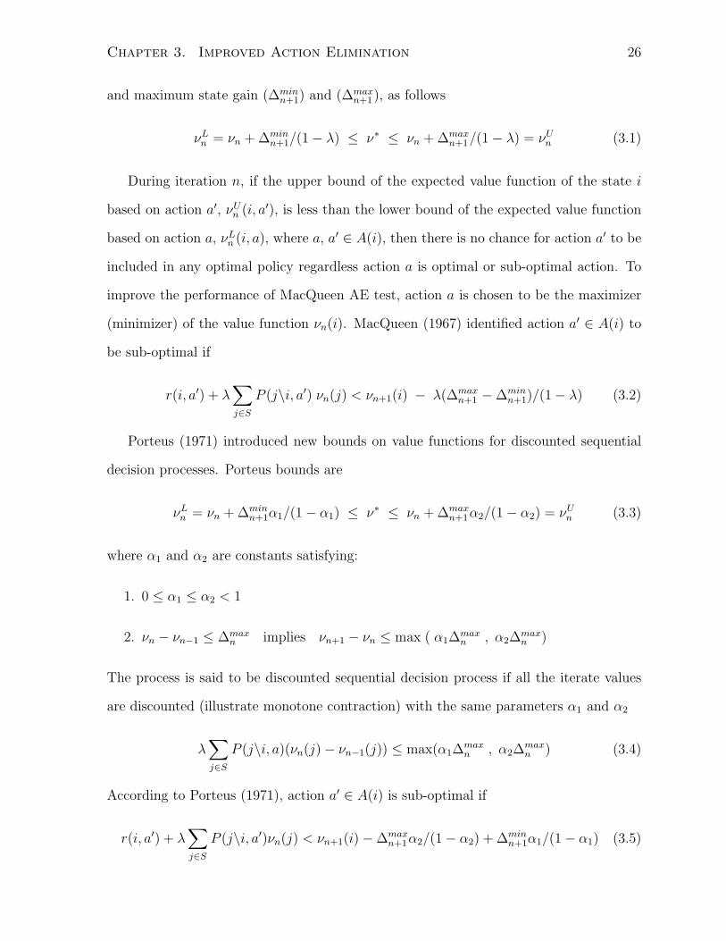
νLn = νn + ∆minn+1/(1− λ) ≤ ν∗ ≤ νn + ∆max

n+1/(1− λ) = νUn (3.1)

During iteration n, if the upper bound of the expected value function of the state i

based on action a′, νUn (i, a′), is less than the lower bound of the expected value function

based on action a, νLn (i, a), where a, a′ ∈ A(i), then there is no chance for action a′ to be

included in any optimal policy regardless action a is optimal or sub-optimal action. To

improve the performance of MacQueen AE test, action a is chosen to be the maximizer

(minimizer) of the value function νn(i). MacQueen (1967) identified action a′ ∈ A(i) to

be sub-optimal if

r(i, a′) + λ∑j∈S

P (j\i, a′) νn(j) < νn+1(i) − λ(∆maxn+1 −∆min

n+1)/(1− λ) (3.2)

Porteus (1971) introduced new bounds on value functions for discounted sequential

decision processes. Porteus bounds are

νLn = νn + ∆minn+1α1/(1− α1) ≤ ν∗ ≤ νn + ∆max

n+1α2/(1− α2) = νUn (3.3)

where α1 and α2 are constants satisfying:

1. 0 ≤ α1 ≤ α2 < 1

2. νn − νn−1 ≤ ∆maxn implies νn+1 − νn ≤ max ( α1∆

maxn , α2∆

maxn )

The process is said to be discounted sequential decision process if all the iterate values

are discounted (illustrate monotone contraction) with the same parameters α1 and α2

λ∑j∈S

P (j\i, a)(νn(j)− νn−1(j)) ≤ max(α1∆maxn , α2∆

maxn ) (3.4)

According to Porteus (1971), action a′ ∈ A(i) is sub-optimal if

r(i, a′) + λ∑j∈S

P (j\i, a′)νn(j) < νn+1(i)−∆maxn+1α2/(1− α2) + ∆min

n+1α1/(1− α1) (3.5)


Hastings and Mello (1973) pointed out that MacQueen’s and Porteus’ tests includes the

terms ∆minn+1 and ∆max

n+1 , which are available at the end of each iteration. Therefore all the

calculated values in the current iteration need to be stored to carry out the elimination

test at the end of each iteration. If the available storage capacity is insufficient these

values need to be recalculated.

Hastings and Mello (1973) suggested using lower and upper bounds on ∆maxn+1 and ∆min

n+1,

respectively, to carry out the AE test as soon as the iterate values are calculated, which

will minimize the storage requirement and eliminates the need to recalculate values. For

the case of stationary, discrete and discounted, finite states and actions, infinite horizon

MDPs, equations (2.24), (2.25) and (2.26) will be reduced to

βi(a) = βn−1

= βn−1 = λ ∀ i ∈ S, a ∈ A(i), n = 1, 2, · · · (3.6)

Hastings’ AE test in (2.23) will be such that action a′ is sub-optimal if

r(i, a′) + λ∑j∈S

P (j\i, a′)νn(j) < νn(i) + λ∆minn /(1− λ)− λ2∆max

n (3.7)

Hubner (1977) improved the upper bound on the convergence rate in the span semi-

norm (α) utilizing the delta coefficient of the composite transition probability matrix (γ),

α ≤ λγ. In addition, Hubner proved that the term λ/(1 − λ) in Porteus test formula

can be replaced by λγ/(1− λγ) or λγi,a/(1− λγ), (Hubner, 1977 and Puterman, 1994),

where:

γ = maxi∈S, a∈A(i), i′∈S, a∈A(i′)

{ 1−∑j∈S

min [ P (j\i, a) , P (j\i′, a) ] } (3.8)

γi,a = maxk∈A(i)

{ 1 −∑j∈S

min [ P (j\i, k) , P (j\i, a) ] } (3.9)

The adaptation of γ and γi,a may improve the AE process by reducing the number of iter-

ations to satisfy the stopping criterion or by eliminating more actions before termination.

Practically, more computational work is needed to calculate and/or update γ and γi,a.

Hubner assessed numerically the value of γ for some tested problems. The performance

of the AE utilizing Hubner’s test was not evaluated. As part of the current research,


numerical studies were conducted to evaluate the effect of γ and γi,a on the performance

of HAE. The results are presented and discussed in section 3.4.

Adopting the AE technique provides an additional stopping criterion that is: if all the

actions are eliminated, except one, for each state i ∈ S, then those remaining actions are

the actions to be selected under the optimal policy. This stopping criterion guarantees

that VI and MPI terminate with an optimal policy instead of ε-optimal policy (Puterman,

1994). In addition, if the desired result is the optimal policy not the optimal value

functions, then termination based on the AE stoping criterion will save the extra effort

and time needed to find the fixed point.

3.2 Norms and VI Schemes Performance

Sup-norm and span semi-norm have been discussed in Chapter 2. Reviewing the

literature, Puterman (1994) (pp. 199) mentioned that convergence to a span fixed point

is often faster than convergence to a norm fixed point for discounted MDPs. Gosavi (2003)

(pp. 180) stated that sometimes the span semi-norm converges much faster than the sup-

norm, then it is a good idea to use the span rather than the sup-norm. Zobel and Scherer

(2005) use the span semi-norm in their numerical studies of the policy convergence when

solving MDPs via successive approximation algorithm. Based on the literature review

conducted during this research, the performance of VI schemes (PJVI, JVI, PGSVI and

GSVI) was not evaluated in the span semi-norm.

In this research, numerical studies are conducted to assess the performance of VI

schemes in both sup-norm and span semi-norm. The main result is that the PJVI al-

gorithm with the span semi-norm stoping criterion demonstrates the best performance

in both the number of iterations and CPUT to converge. Therefor, we will adopt it as

the successive approximation framework for introducing the IAE algorithm, comparing

it with other algorithms, and conducting all the numerical studies.


3.3 Action Gain and Action Relative Gain

New terms, such as action gain, action relative gain and cumulative action relative gain,

are introduced in this research to set the foundation for the improved AE algorithm. For

any action a ∈ A(i), define the gain of action a during iteration n + 1 (AGan+1(i)) such

that:

AGan+1(i) = [ r(i, a)+λ

∑j∈S

P (j\i, a)νn(j) ] − [ r(i, a)+λ∑j∈S

P (j\i, A)νn−1(j) ] (3.10)

Rearrange the terms to get

AGan+1(i) = λ

∑j∈S

P (j\i, a) ∆n(j) (3.11)

AGan+1(i) is a measure of the improvement in the iterate value function based on action

a ∈ A(i) during the iteration n + 1. Define the relative gain of action a compared to

action a (ARGa,an+1(i)), a, a ∈ A(i), such that

ARGa,an+1(i) = AGa

n+1(i)− AGan+1(i) (3.12)

ARGa,an+1(i) measures the difference in the improvement of ν(i, ·) based on the actions

a , a ∈ A(i) during the iteration n + 1. Define the action cumulative relative gain

(ACRGa,an+1(i)) such that

ACRGa,an+1(i) =

∞∑l=1

ARGa,an+l(i) (3.13)

ACRGa,an+1(i) is the cumulative difference in the improvement in ν(i) based on two differ-

ent actions a and a in A(i) starting from iteration n + 1 until convergence to the fixed

point. The following Lemma provides an upper bound on the action cumulative relative

gain. This bound will be essential in deriving the IAE algorithm.

Lemma 3.1: For any stationary discounted MDP, a and a ∈ A(i), i ∈ S and n ≥ 1,

an upper bound of the action cumulative relative gain is such that

ACRGa,an+1(i) ≤ Sn λγ

i,a,a/(1− λ) (3.14)


where:

γi,a,a = 1 −∑j∈S

min [ P (j\i, a) , P (j\i, a) ] (3.15)

Sn = ∆maxn − ∆min

n (3.16)

proof:

By definition

ARGa,an+1(i) = λ

∑j∈S

P (j\i, a) ∆n(j)− λ∑j∈S

P (j\i, a) ∆n(j)

= λ∑j∈S

( P (j\i, a) − min [ P (j\i, a) , P (j\i, a) ] )∆n(j)

−λ∑j∈S

( P (j\i, a) − min [ P (j\i, a) , P (j\i, a) ] )∆n(j)

≤ λ ( 1 −∑j∈S

min [ P (j\i, a) , P (j\i, a) ] )∆maxn

−λ ( 1 −∑j∈S

min [ P (j\i, a) , P (j\i, a) ] )∆minn

= λ γi,a,a ( ∆maxn −∆min

n ) = λ γi,a,a Sn

By definition

ACRGa,an+1(i) =

∞∑l=1

ARGa,an+l(i) ≤ λ γi,a,a

∞∑l=1

Sn+l−1 = λ γi,a,a∞∑l=0

Sn+l

Based on contraction property of the span semi-norm (Theorem 6.6.6 (pp.202) Puterman,

1994)

Sn+l ≤ λlSn, l = 1, 2, · · ·

Then

ACRGa,an+1(i) ≤ λ γi,a,a

∞∑l=0

λlSn = Sn λ γi,a,a/(1− λ) �


3.4 Improved Action Elimination Algorithm

The first objective in this research is to improve the AE for a class of MDPs that have

one discounting factor λ, for which Portues’ discounting factors α1 = α2 = λ. Therefore

MacQueen’s and Porteus’ bounds are identical. Porteus bounds and AE test are reduced

to be:

νLn = νn + ∆minn λ/(1− λ) ≤ ν∗ ≤ νn + ∆max

n λ/(1− λ) = νUn (3.17)

and action a′ ∈ An(i) is sub-optimal if

r(i, a′) + λ∑j∈S

P (j\i, a′)νn(j) < νn+1(i) + Sn+1λ/(1− λ) (3.18)

Where An(i) is the set of non-eliminated actions in state i at the beginning of iteration

n. The main contribution of this chapter is that in the improved AE test stated in

Theorem 3.1 below; the factor γi,a′,a∗n(i) replaces the factor γi,a′ suggested by Hubner

(1977), where a∗n(i) is the maximizing (best) action of state i in iteration n.

Theorem 3.1: For any stationary discounted MDP, if

νn(i) > r(i, a′) + λ∑j∈S

P (j\i, a′)νn−1(j) + Snλγi,a′,a∗n(i)/(1− λ) (3.19)

then the action a′ ∈ An(i) is sub-optimal and can be eliminated from Am(i) ∀ m > n,

where:

γi,a′,a∗n(i) = 1 −

∑j∈S

min [ P (j\i, a′) , P (j\i, a∗n(i)) ] (3.20)

a∗n(i) ∈ arg maxa∈An(i)

{ r(i, a) + λ∑j∈S

P (j\i, a)νn−1(j) } (3.21)

An(i) is the set of non-eliminated actions in state i at the beginning of iteration n.

proof:

By definition

νn(i) = r(i, a∗n(i)) + λ∑j∈S

P (j\i, a∗n(i))νn−1(j)


If

νn(i) > r(i, a′) + λ∑j∈S

P (j\i, a′)νn−1(j) + ACRGa′,a∗n(i)n+1 (i)

then there is no chance for action a′ to outperform action a∗n(i), which means a′ is sub-

optimal action that can be eliminated. Replacing ACRGa′,a∗n(i)n+1 (i) by its upper bound in

Lemma 1, it follows that

νn(i) > r(i, a′) + λ∑j∈S

P (j\i, a′)νn−1(j) + Snλγi,a′,a∗n(i)/(1− λ) �

The suggested terms γi,a′,a∗n(i) have two main advantages compared to Hubner’s terms

γi,a. The first advantage is that γi,a′,a∗n(i) makes the inequality (3.18) easier to be satisfied

and accordingly improves the AE, which is obvious since

γi,a = maxa′∈A(i)

{γi,a′,a} (3.22)

The second advantage is that the computational effort needed to calculate γi,a,a∗n(i) for

all a ∈ An(i) is less than that needed to calculate γi,a. Later, as more actions are

eliminated the term γi,a can be improved (reduced) at a cost of additional computations,

while the terms γi,a′,a∗n(i) do not need updating since there is no room for improvement.

Most likely the new AE test will eliminate sub-optimal actions earlier. Reducing the

computational effort and eliminating sub-optimal actions in fewer iterations will improve

the performance of AE technique and accelerate the successive approximation algorithm

when solving MDPs.

A flow chart diagram for the suggested IAE algorithm is presented in Figure (3.1). As

can be seen the algorithm terminates successfully based on any of two stopping criteria

which ever satisfied first. The IAE algorithm is a modification of the PJVI algorithm,

discussed in Chapter 2, to adopt the new AE test suggested in Theorem 3.1 in this

research. It is anticipated that this algorithm will outperforms Hubner’s AE algorithm

and speeds up the successive approximation algorithm. Following is detailed description

of the IAE algorithm


Figure 3.1: Flow chart diagram for the IAE algorithm


IAE Algorithm:

Step 1. Initialization: Select ν0 ∈ V , specify ε > 0 and set n = 1.

Step 2. Value functions improvement: ∀ i ∈ S, compute νn such that

νn(i) = maxa∈An(i)

{ r(i, a) + λ∑j∈S

P (j\i, a)νn−1(j) },∀ i ∈ S

where An(i) is the set of non-eliminated actions in state i at the beginning of

iteration n, A1(i) = A(i).

Step 3. check for span semi-norm stopping criterion: If Sn < ε (1 − λ)/λ, go to

step 7; otherwise continue to step 4.

Step 4. Action elimination: ∀ i ∈ S, a′ ∈ An(i), if

νn(i) > r(i, a′) + λ∑j∈S

P (j\i, a′)νn−1(j) + Snλγi,a′,a∗n(i)/(1− λ)

then action a′ is sub-optimal action and can be eliminated, where

γi,a′,a∗n(i) = 1−

∑j∈S

min[P (j\i, a∗n(i)), P (j\i, a′)]

a∗n(i) ∈ arg maxa∈An(i)

{r(i, a) + λ∑j∈S

P (j\i, a)νn−1(j)}

Step 5. Check for AE stopping criterion: If |An+1(i)| = 1 for each i ∈ S continue

to step 6; otherwise increment n by 1 and go back to step 2.

Step 6. Optimal policy identification: Set d∗ such that d∗(i) = An+1(i) and STOP.

Step 7. Identifying ε-optimal policy: For each i ∈ S


n )/2(1− λ)


d∗ε(i) ∈ arg maxa∈An(i){r(i, a) + λ∑j

P (j\i, a)ν∗span(j)}.

3. STOP


3.5 Numerical Studies

To validate the direction and the effectiveness of the suggested improvements, different

numerical studies are carried out to:

1. Compare the performance of the successive approximation schemes in both sup-

norm and span semi-norm.

2. Evaluate the effectiveness of the term γ used in Hubner’s bounds and AE test.

3. Compare the performance of Hubner’s, Porteus’s and Improved AE algorithms.

Few points to be mentioned prior to presenting and discussing results of the various

numerical studies:

1. The transition probabilities and the one step rewards in all the tested problems are

randomly generated.

2. In order to avoid reducibility, the TPM for any policy contains an upper and a

lower diagonals with non-zero entries.

3. The tolerance (ε) was fixed, ε = 0.00001, through all numerical studies.

4. Abbreviations used to present results are summarized in Table (3.1)

Random MDPs Generation:

The performance assessment of the proposed algorithms will utilize randomly gener-

ated MDPs as follows:

• The number of non-zero entries in each raw of the transition probability matrix is

selected randomly to be within a range relevant to the TPMS.

• The non-zero entries are generated randomly, normalized and assigned to different

columns (possible next states) randomly.


Table 3.1: Abbreviations used in numerical studies

Abbreviation Parameter Description

N Number of iterations in span semi-norm

AN Average number of iterations in span semi-norm

ND Number of iterations standard deviation in span semi-norm

Nsup Number of iterations in sup-norm

ANsup Average number of iterations in sup-norm

NDsup Number of iterations standard deviation in sup-norm

AT Average CPU time

ANS% Average savings percentage in number of iterations

ATS% Average savings percentage in CPU time

AAPS Average number of admissible actions per state

NFT Number of tested problems with solution different than that in PJVI

• The one step reward (cost) for each state and action is generated randomly to be

within specified rang.

All the random numbers are generated according to the uniform distribution.

Numerical Studies I:

The first group of numerical studies were conducted to assess the performance of the

successive approximation schemes (PJVI, JVI, PGSVI and GSVI) in both the sup-norm

and the span semi-norm. Randomly generated MDPs with: |S| = 100, AAPS = 10,

TPMS = 0.25, 0.50, 0.75, 0.90, 0.95, λ = 0.80, 0.90, 0.95, 0.99. Figures (3.2) and (3.3)

present obtained results in terms of number of iterations to converge for two cases of λ

(0.80 and 0.99), respectively.

For PJVI, it is clear that Nsup is insensitive to TPMS, while it is extremely sensitive

to λ especially when it is close to 1. On the contrary N is more sensitive towered TPMS

compared to λ. In the case of JVI, the Nsup decreases and N increases as TPMS increase,

for PGSVI and GSVI both Nsup and N increases and decreases as TPMS increase, re-


Figure 3.2: VI schemes performance in AN (λ = 0.80)

spectively. Adopting span semi-norm stopping criteria improved the performance of all

the schemes in terms of AN and AT to converge with different extents. The minimum

improvement was in the case of GSVI while the maximum improvement was in the PJVI.

The trends in Nsup and N are identical in Figures (3.2) and (3.3) for λ = 0.80 and 0.99,

respectively. Figures (3.4) and (3.5) present the results in terms of CPUT to converge,

the same behavior of the schemes with respect to TPMS and λ noticed in Figures (3.2)

and (3.3) is repeated in Figures (3.4) and (3.5). All the cases of λ demonstrate the same

behavior with different scale, λ = 0.80 and 0.98 were selected to show the range of the

obtained results in AN and AT. Detailed statistics for the numerical studies results are

presented in Tables A.1, A.2, A.3 and A.4 in the Appendix for PJVI, JVI, PGSVI and

GSVI, respectively.


Figure 3.3: VI schemes performance in AN (λ = 0.99)

Figure 3.4: VI schemes performance in AT (λ = 0.80)


Figure 3.5: VI schemes performance in AT (λ = 0.99)

Based on numerical results presented in Figures (3.2), (3.3), (3.4) and (3.5), it is found

that:

1. The span semi-norm improve the performance of all the successive approximation

schemes in both AN and AT to converge.

2. The PJVI was ranked last in the sup-norm and first in the span semi-norm in both

AN and AT to converge.

Numerical results shows that the PJVI with span semi-norm stopping criterion demon-

strated an exceptional performance in both AN and AT , therefor it will be the successive

approximation framework for introducing the improved AE algorithm, comparing it with

other algorithms and for conducting all the numerical studies.

Numerical Studies II:

To assess the effectiveness of the coefficient γ used by Hubner to improve the perfor-

mance of AE, γ was calculated for 100 randomly generated MDPs for each (TPMS,|S|)

combination, TPMS = 0.98, 0.95, 0.90, 0.75, 0.5 and 0.25, |S| = 100, 200 and 500, and


Table 3.2: Average values for γ

Average γTPMS |S|=100 |S|=200 |S|=500

0.98 1.000 1.000 1.0000.95 1.000 1.000 1.0000.90 1.000 1.000 1.0000.75 0.998 0.987 0.9490.50 0.853 0.814 0.7670.25 0.651 0.614 0.576

AAPS = 10. The average value of the coefficient γ for each setting of TPMS and prob-

lem size are presented in Table (3.2) which demonstrates that γ increases as the TPMS

increase or the problem size decrease. All the tested MDPs with TPMS ≥ 0.90 returns

γ = 1.00. For the case of TPMS = 0.75, the average value of γ was 0.998, 0.987 and 0.949

for |S| = 100, 200 and 500, respectively, which is very close to 1. When γ = 1 Hubner’s

and Portues bounds are identical and will have the same performance in terms of AN ,

while in terms of AT Portues will performs better due to CPUT spent in calculating γ.

Numerical studies were conducted to evaluate the performance of Hubner’s AE (HAE1)

algorithm and to compar it with PAE algorithm. 100 randomly generated MDPs with

|S| = 100 and AAPS = 30 were solved using both PAE and HAE1 for each (λ , TPMS)

combination, λ = 0.80, 0.90, 0.95 and 0.99, TPMS = 0.10, 0.50, 0.80 and 0.90. The

performance is measured in AN and AT which are presented in Table (3.3), detailed

statistics of the numerical studies results are presented in Table A.5 in the Appendix.

The results in Table (3.3) shows zero savings in AN for the cases with TPMS ≥ 0.80,

which is a direct subsequence for the previous result that γ = 1 for these cases. The

maximum ANS% was 26.77% for the case with λ = 0.99 and TPMS = 0.10. 0.99 is the

maximum tested value of λ at which the term λ/(1 − λ) has its maximum value and

Portues’ bounds are very loss deteriorating the performance of PAE algorithm. On the

average, the value of γ decreases as the TPMS decrease, which improves the performance


Table 3.3: Performance of PAE and HAE1 in AN and AT (|S|=100)

PAE HAE1λ TPMS AN AT AN AT ANS% ATH1/ATP

0.8 0.1 4.99 0.009 4.37 19.078 12.42 2119.780.5 5.76 0.01 5.44 16.645 5.56 1664.500.8 7.01 0.011 7.01 0.012 0 1.090.9 8.5 0.013 8.5 0.013 0 1.00

0.9 0.1 5.45 0.01 4.61 19.073 15.41 1907.300.5 6.39 0.011 6.01 16.648 6.10 1513.460.8 8.08 0.014 8.08 0.016 0 1.140.9 9.74 0.015 9.74 0.015 0 1.00

0.95 0.1 5.63 0.011 4.51 19.083 19.89 1734.820.5 6.98 0.012 6.32 16.652 9.455 1387.670.8 9.03 0.015 9.03 0.016 0 1.070.9 11.34 0.018 11.34 0.018 0 1.00

0.99 0.1 6.35 0.013 4.65 19.087 26.77 1468.230.5 7.71 0.015 6.36 16.644 17.50 1109.600.8 10.14 0.018 10.14 0.02 0 1.110.9 13.26 0.024 13.26 0.024 0 1.00

of HAE1 in terms of AN . In terms of CPUT, the results show that HAE1 takes at least

the same time that PAE needs to terminate. It is the same time for the cases with TPMS

= 0.90, for which it will take a very sort time (almost zero) to find the first (i, a) and

(i′, a′) that returns γ = 1. Then HAE1 and PAE tests are identical and the two algorithms

needs the same number of iterations and CPUT to converge. For the cases with TPMS =

0.50 and 0.10, HAE1 will terminates in less number of iterations, unfortunately it needs

mach more time to converge, the AT for HAE1 was more than 1100 folds of that for PAE

for all the tested problems with TPMS ≤ 0.50, for some cases it was up to 2119.74 folds.

This is mainly due to the fact that calculating γ is extremely expensive, it is exponential

in both AAPS and |S|. It requires |S|(|S|+ 1)∑

i∈S∑

j∈S |A(i)||A(j)| compressions and

additions to return γ < 1.

AN versus TPMS has the same pattern for all the values of λ, which is true for AT

versus TPMS as well. As sample, Figures (3.6) and (3.7) show the behavior of AN and


Figure 3.6: Performance of PAE and HAE1 in AN (|S| = 100)

AT versus TPMS for the case of λ = 0.80 and 0.99, respectively.

Numerical Studies III:

In this research, a new AE (IAE) algorithm is introduced. Numerical studies were

conducted to assess and compare the performance of the IAE with other algorithms,

explicitly PAE and a modified version of Hubner’s AE (HAE2) in which the coefficient

γ is dropped. The HAE2 algorithm utilize the following formula to test for AE

νn(i) > r(i, a′) + λ∑j∈S

P (j\i, a′)νn−1(j) + Snλγi,a∗n(i)/(1− λ) (3.23)

A 100 randomly generated MDPs with |S| = 200 and AAPS = 30 for each of the λ

and TPMS combinations, λ = 0.80, 0.90, 0.95 and 0.99, TPMS = 0.10, 0.50, 0.80, 0.90,

0.95 and 0.98, are solved using PAE, HAE2 and IAE. Figures (3.8) and (3.9) show the

behavior of AN versus TPMS and AT versus TPMS for two values of λ (0.80 and 0.99),

respectively. AN versus TPMS and AT versus TPMS has the same trends for each tested

value of λ, the results of the smallest and largest λ are selected to be presented. Detailed

statistics of the numerical studies results AN and AT are presented in Tables A.6 and


Figure 3.7: Performance of PAE and HAE1 in AT (|S| = 100)

A.7 in the Appendix, respectively.

Figure (3.8) shows that the AN of the three algorithms are very close for a fixed

λ. The results in Table A.6 demonstrated that ANIAE < ANHAE1 < ANPAE, which

is an expected result. In terms of AT , although IAE outperformed HAE2 in all the

tested problems, unfortunately, PAE is the best as clearly presented in Figure (3.9). A

hypothesis test is conducted to asses the chance for IAE to perform as good as PAE in

terms of computational time. The hypothesis are set such that:

H0 : µI − µP = 0 (3.24)

H1 : µI − µP > 0 (3.25)

The null hypothesis was rejected with 0.999 confidence level for all the (λ, TPMS)

tested values.


Figure 3.8: Performance of PAE, HAE2 and IAE in AN (|S| = 200)

Figure 3.9: Performance of PAE, HAE2 and IAE in AT (|S| = 200)


3.6 Conclusion

The successive approximation schemes were assessed in both sup-norm and span semi-

norm using randomly generated MDPs with different levels of TPMS and values of λ. The

numerical results obtained shows that the PJVI with span semi-norm stopping criterion

is the best performer in both AN and AT to converge. Therefor, we adopt the PJVI with

the span semi-norm through out this research. The performance of Hubner’s AE (HAE1)

was assessed and compared to Portues’ AE (PAE), the results were disappointing; either

γ = 1 or it is extremely expensive in terms of CPUT to return γ < 1. A modified version

of HAE1 that dropped the coefficient γ to eliminate its computational complexity was

suggested to assess the effectiveness of Hubner’s terms γi,a in comparison with the new

terms γi,a,a∗n(i) used in the improved AE (IAE) algorithm. In terms of AN to converge,

IAE shows the best performance and MAE2 outperformed PAE. In terms of AT , although

HAE2 performed much better than HAE1 and IAE performed better than HAE2, PAE

was the best. However, there is a room for improvement.

As a result of this investigation, it can be said that some more work to minimize

computational effort required to calculate γi,a′,a∗n(i) is needed so that the savings in number

of iterations is reflected as savings in CPUT. For some structured MDPs like queueing

systems, where the set of relevant next states are the same for any state i ∈ S regardless

of the action to be selected; Calculating γi,a′,a∗n(i) will be less expensive. Most likely, the

values of γi,a′,a∗n(i) will be smaller which will improve the performance of the IAE. This

part is left for future research.

Chapter 4

Heuristic Action Elimination

Most exact AE algorithms proposed for discrete and discounted MDPs utilizes the dis-

counting factor λ as an upper bound on the convergence rate (MacQueen, 1967; Porteus,

1971; Grinold, 1973; Hastings and Mello, 1973 and Hastings, 1976). Hubner (1977) sug-

gested using γλ as upper bound on the convergence rate; unfortunately, numerical results

in Chapter 3 demonstrated that Hubner’s bound may not be useful since it is computa-

tionally very expensive to get γ < 1. It is well known that the convergence in the first

few iterations of the successive approximation is much faster than the long run conver-

gence (White and Scherer, 1994 and Puterman, 1994). This motivated current research

to evaluate numerically the behavior of actual convergence in successive approximation in

both sup-norm and span semi-norm. The numerical results demonstrated that the actual

convergence in span semi-norm is faster than the known theoretical rate. The absence of

easy-to-compute bounds on the actual convergence rate motivated the current research

to try a heuristic AE (HAE) algorithm. The heuristic utilizes an estimated convergence

rate seeking speeding up successive approximation and maintaining solution optimality

or ε-optimality.

46

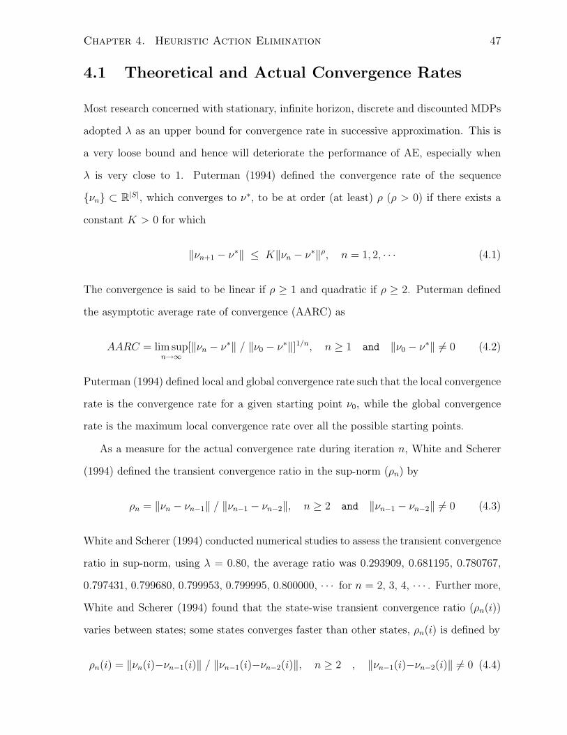
Chapter 4. Heuristic Action Elimination 47

4.1 Theoretical and Actual Convergence Rates

Most research concerned with stationary, infinite horizon, discrete and discounted MDPs

adopted λ as an upper bound for convergence rate in successive approximation. This is

a very loose bound and hence will deteriorate the performance of AE, especially when

λ is very close to 1. Puterman (1994) defined the convergence rate of the sequence

{νn} ⊂ R|S|, which converges to ν∗, to be at order (at least) ρ (ρ > 0) if there exists a

constant K > 0 for which

‖νn+1 − ν∗‖ ≤ K‖νn − ν∗‖ρ, n = 1, 2, · · · (4.1)

The convergence is said to be linear if ρ ≥ 1 and quadratic if ρ ≥ 2. Puterman defined

the asymptotic average rate of convergence (AARC) as

AARC = lim supn→∞

[‖νn − ν∗‖ / ‖ν0 − ν∗‖]1/n, n ≥ 1 and ‖ν0 − ν∗‖ 6= 0 (4.2)

Puterman (1994) defined local and global convergence rate such that the local convergence

rate is the convergence rate for a given starting point ν0, while the global convergence

rate is the maximum local convergence rate over all the possible starting points.

As a measure for the actual convergence rate during iteration n, White and Scherer

(1994) defined the transient convergence ratio in the sup-norm (ρn) by

ρn = ‖νn − νn−1‖ / ‖νn−1 − νn−2‖, n ≥ 2 and ‖νn−1 − νn−2‖ 6= 0 (4.3)

White and Scherer (1994) conducted numerical studies to assess the transient convergence

ratio in sup-norm, using λ = 0.80, the average ratio was 0.293909, 0.681195, 0.780767,

0.797431, 0.799680, 0.799953, 0.799995, 0.800000, · · · for n = 2, 3, 4, · · · . Further more,

White and Scherer (1994) found that the state-wise transient convergence ratio (ρn(i))

varies between states; some states converges faster than other states, ρn(i) is defined by

ρn(i) = ‖νn(i)−νn−1(i)‖ / ‖νn−1(i)−νn−2(i)‖, n ≥ 2 , ‖νn−1(i)−νn−2(i)‖ 6= 0 (4.4)


Following White and Scherer (1994), we define transient and maximum convergence

ratios in the sup-norm, (λn) and (λmax), respectively, such that

λn = ‖νn − νn−1‖ / ‖νn−1 − νn−2‖, 2 ≤ n ≤ N (4.5)

where N is the smallest integer for which ‖νN − νN−1‖ < ε(1− λ)/2λ

λmax = max2≤n≤N

{λn} (4.6)

Similarly, define transient and maximum convergence ratios in the span semi-norm, (αn)

and (αmax), respectively, such that

αn = sp (νn − νn−1) / sp (νn−1 − νn−2), 2 ≤ n ≤ N (4.7)

where N is the smallest integer that satisfy sp (νN − νN−1) < ε(1− λ)/λ

αmax = max2≤n≤N

{αn} (4.8)

Since λ and λγ are upper bounds on the convergence rate in the sup-norm and span

semi-norm, respectively, the following two relations will hold for 2 ≤ n ≤ N

λn ≤ λmax ≤ λ (4.9)

αn ≤ αmax ≤ λγ ≤ λ (4.10)

In order to assess λmax and αmax, numerical studies were conducted. Randomly

generated MDPs with |S| = 200, AAPS = 10, λ = 0.80, 0.90, 0.95 and 0.99, TPMS =

0.25, 0.50, 0.75, 0.90, 0.95 and 0.98, were solved using PJVI. The average λmax, αmax

and γ of 100 problem for each (λ , TPMS) are presented in Table (4.1). The results

demonstrate that λmax = λ for all the tested problems. This result coincides with White

and Scherer (1994) results indicating that there is no room to improve the upper bound

on convergence rate in the sup-norm. Table (4.1) demonstrates that αmax < λγ for all

the tested problems. αmax decreases as the TPMS decreases. The rate at which αmax

decreases is much faster than that of γ; the ratio (αmax/λγ) decreases as TPMS decreases.


Table 4.1: Average values for λmax, αmax, γ and the ratio αmax/λγ

λ TPMS λmax αmax γ αmax/λγ

0.99 0.98 0.990 0.823 1.000 0.831

0.95 0.990 0.479 1.000 0.484

0.90 0.990 0.324 1.000 0.327

0.75 0.990 0.193 0.987 0.198

0.50 0.990 0.125 0.814 0.155

0.25 0.990 0.086 0.614 0.141

0.95 0.98 0.950 0.781 1.000 0.822

0.95 0.950 0.455 1.000 0.479

0.90 0.950 0.308 1.000 0.324

0.75 0.950 0.183 0.989 0.195

0.50 0.950 0.117 0.816 0.151

0.25 0.950 0.085 0.616 0.145

0.90 0.98 0.900 0.741 1.000 0.823

0.95 0.900 0.428 1.000 0.476

0.90 0.900 0.287 1.000 0.319

0.75 0.900 0.177 0.988 0.199

0.50 0.900 0.112 0.816 0.153

0.25 0.900 0.080 0.615 0.145

0.80 0.98 0.800 0.652 1.000 0.815

0.95 0.800 0.381 1.000 0.476

0.90 0.800 0.256 1.000 0.320

0.75 0.800 0.156 0.989 0.197

0.50 0.800 0.100 0.815 0.153

0.25 0.800 0.072 0.616 0.146


4.2 Estimated Convergence Rate

Providing a theoretical upper bound on α that supports the numerical results presented

in Table (4.1) is still a challenge. This motivated a heuristical AE to use a dynamic

estimated convergence rate (αIn). The average of most recent transient convergence ratio

αn and the upper bound λ is used to estimate the convergence rate α which will replace

λ in Porteus AE test.

αIn = (αn + λ)/2 = (λSn−1 + Sn)/2Sn−1 (4.11)

Other estimate, which is a bit more greedy, is

αIIn = λSn−1/((1 + λ)Sn−1 − Sn) (4.12)

Table (4.2) compares αIn and αIIn for different values of αn and λ. It shows that αIIn < αIn

when αn < λ and αIIn = αIn = λ if αn = λ.

The algorithm terminates based on the span semi-norm stopping criterion when SN <

ε(1− λ)/λ, then Sn ≥ ε(1− λ)/λ for all n < N . Combining this fact with the definition

of αIIn provides a lower bound on αIIn

αIIn = λSn−1/((1 + λ)Sn−1 − Sn) ≥ λSn−1/((1 + λ)Sn−1) = λ/(1 + λ) (4.13)

4.3 Heuristic Action Elimination Algorithm

Improving the bound on convergence rate is a very effective approach to improve and

accelerate AE. αIIn provides an estimation of the convergence rate in the span semi-norm

which is less than λ. The IAE algorithm proposed in chapter 3 is modified to adopt

αIIn , the term λγi,a′,a∗

n /(1 − λγ) is replaced with λ/(1 − αn) in the AE test in step 3,

where αn = αIIn . Following is detailed description of the suggested heuristic AE (HAE)

algorithm.


Table 4.2: comparison of αIn and αIIn

λ = 0.90 λ = 0.95 λ = 0.99

α αIn αIIn αIn αIIn αIn αIIn

0.20 0.550 0.529 0.575 0.543 0.595 0.553

0.30 0.600 0.563 0.625 0.576 0.645 0.586

0.40 0.650 0.600 0.675 0.613 0.695 0.623

0.50 0.700 0.643 0.725 0.655 0.745 0.664

0.60 0.750 0.692 0.775 0.704 0.795 0.712

0.70 0.800 0.750 0.825 0.760 0.845 0.767

0.80 0.850 0.818 0.875 0.826 0.895 0.832

0.90 0.900 0.900 0.925 0.905 0.945 0.908

0.91 0.930 0.913 0.950 0.917

0.92 0.935 0.922 0.955 0.925

0.93 0.940 0.931 0.960 0.934

0.94 0.945 0.941 0.965 0.943

0.95 0.950 0.950 0.970 0.952

0.96 0.975 0.961

0.97 0.980 0.971

0.98 0.985 0.980

0.99 0.990 0.990


HAE Algorithm

Step 1. Initialization: Select ν0 ∈ V , specify ε > 0 and set n = 1

Step 2. Value functions improvement: ∀ i ∈ S, a ∈ An(i), compute νn(i) such that

νn(i) = maxa∈An(i)

{ r(i, a) + λ∑j∈S

P (j\i, a)νn−1(j) },∀ i ∈ S

where An(i) is the set of non-eliminated actions in state i at the beginning of

iteration n, A1(i) = A(i).

step 3: Check for span semi-norm stopping criterion: If Sn < ε (1− λ)/λ, go to

step 7; otherwise continue to step 4.

step 4. Action elimination: ∀ i ∈ S, a′ ∈ An(i), if

νn(i) > r(i, a′) + λ∑j∈S

P (j\i, a′)νn−1(j) + Snλ/(1− αn)

then action a′ is a sub-optimal action and must be eliminated, where

αn = λSn−1/((1 + λ)Sn−1 − Sn)

step 5. Check for AE stopping criterion: If |An+1(i)| = 1 ∀ i ∈ S continue to

step 6; otherwise increment n by 1 and go back to step 2.

step 6. Optimal policy identification: Set d∗ such that d∗(i) = An+1(i) and STOP.

Step 7: ε-optimal policy identification: For each iinS

1. Set ν∗span such that ν∗span(i) = νn(i) + (∆maxn + ∆min

n )/2(1− λ), where


d∗ε(i) ∈ arg maxa∈An(i)

{r(i, a) + λ∑j

P (j\i, a)ν∗span(j)}

3. STOP

The HAE algorithm is tested and compared to PAE algorithm, the results are pre-

sented and discussed in the next section.



The performance of the suggested HAE was tested using randomly generated MDPs.

Problems with |S| = 200, AAPS = 20, λ = 0.80, 0.90, 0.95 and 0.99, TPMS = 0.80,

0.90, 0.95 and 0.98, were solved using both PAE and HAE algorithms. The AN and

AT of 1000 tested problems solved for each (λ , TPMS) combination are presented in

Table(4.3). Detailed statistics for the numerical studies results are listed in Table A.8 in

the Appendix. The HAE shows outstanding performance in terms of solution optimality,

it found the optimal policy for all the tested problems. In terms of savings in number of

iterations and CPUT, the ANS% was in the range 10.93% to 60.35% and the ATS% was

in the range of 77.13% to 91.04%. Figures (4.1) and (4.2) compare the performance of

PAE and HAE in terms of AN and AT, respectively.

Numerical results in Table(4.3) demonstrate that αmax < λ/(1 + λ) ≤ αIIn for all the

tested problems with TPMS ≤ 0.95, which may explains the exceptional performance

of the HAE in terms of solution optimality for these cases, however, HAE and PAE

returns the same solution for all the tested problems with TPMS = 0.98. The obtained

results indicate that there is a room for more greedy estimates of α that improve AE and

accelerate successive approximation algorithm, this part is left for future research.


Table 4.3: Performance evaluation of HAE compared to PAE (|S|=200)

PAE HAE

λ TPMS AN AT AN AT ANS% ATP/ATH

0.99 0.98 31.32 0.5147 22.36 0.1165 28.60 4.42

0.95 14.20 0.4617 10.41 0.0808 26.68 5.71

0.9 10.73 0.4707 8.03 0.0734 25.19 6.41

0.8 8.84 0.5071 6.72 0.0691 23.97 7.34

0.5 7.06 0.6136 5.42 0.0666 23.25 9.21

0.1 5.68 0.6846 4.39 0.0634 22.79 10.80

0.95 0.98 24.49 0.4715 20.05 0.1079 18.12 4.37

0.95 12.07 0.4460 9.96 0.0785 17.54 5.68

0.9 9.43 0.4591 7.85 0.0720 16.73 6.38

0.8 7.83 0.4987 6.61 0.0675 15.65 7.38

0.5 6.30 0.6062 5.36 0.0658 15.02 9.22

0.1 5.14 0.6811 4.32 0.0634 16.01 10.75

0.9 0.98 20.73 0.4516 18.03 0.0997 12.99 4.53

0.95 10.97 0.4381 9.55 0.0760 12.94 5.76

0.9 8.71 0.4543 7.62 0.0698 12.52 6.51

0.8 7.32 0.4932 6.45 0.0659 11.92 7.48

0.5 5.92 0.6043 5.23 0.0650 11.68 9.30

0.1 4.90 0.6772 4.28 0.0627 12.71 10.79

0.8 0.98 15.68 0.4307 14.33 0.0870 8.65 4.95

0.95 9.33 0.4287 8.57 0.0712 8.06 6.02

0.9 7.67 0.4482 7.07 0.0661 7.81 6.78

0.8 6.63 0.4896 6.14 0.0631 7.35 7.76

0.5 5.40 0.5994 5.05 0.0632 6.34 9.48

0.1 4.46 0.6680 4.20 0.0609 5.81 10.97


Figure 4.1: Performance of P-AE and H-AE (AN vis TPMS)

Figure 4.2: Performance of P-AE and H-AE (AT vis TPMS)


4.5 Conclusion

The transient and the maximum convergence ratios in both sup-norm and span semi-norm

were defined and tested to measure the actual convergence in successive approximation.

The numerical results demonstrated that the actual maximum convergence ratio in the

sup-norm is equal to λ. For the span semi-norm, the numerical results demonstrated that

the actual maximum convergence ratio is much smaller than the best known upper bound

on the convergence rate α. The lack of easy-to-compute bounds on the actual convergence

rate motivated the current research to try a heuristic AE (HAE) algorithm. The HAE

utilized an estimated convergence rate which accelerated successive approximation up

to 10.97 folds faster than PAE while maintaining solution optimality or ε-optimality.

The obtained results suggest more greedy estimates, this is highly recommended when

time availability is very limited where fast near-optimal solution is much better than late

optimal or ε-optimal solution.

Chapter 5

Action Elimination for Monotone

Policy MDPs

Monotone policy MDPs (MPMDPs) enjoy a nice property which is utilized to improve

the performance of algorithms and techniques used to solve MPMDPs (Heyman and So-

bel, 1984 and Puterman, 1994). The current research proposes state space partitioning

and state prioritization to employ the monotonicity of optimal policy in a way that max-

imizes the elimination of sub-optimal actions to accelerate the successive approximation

algorithm when solving MPMDPs.

5.1 Monotone Policy MDPs

Structured MDPs are discussed in the literature as a special class of MDPs which has

certain properties or characteristics that can be utilized to accelerate solving these MDPs

(Serfozo, 1976; White, 1981; Heyman and Sobel, 1984; Amir and Hadim, 1992; Puter-

man, 1994), MPMDPs are examples of structured MDPs. Many problems are known

to have monotone optimal policy; such problems are very common in queueing systems,

maintenance management and inventory control among other applications. Topkis is one

of the leading researchers in this area (Topkis, 1968; 1978 and 1998). In his Ph.D. dis-

57

Chapter 5. Action Elimination for Monotone Policy MDPs 58

sertation he discussed the optimality of ordered solutions and presented the first general

framework for monotone optimal policies (Topkis, 1968). Serfozo (1981) established the

optimality of monotone policies for special classes of MDPs such as random walks, birth

and death processes and M/M/s queues. Serfozo (1981) shows that, under certain con-

ditions, M/M/s queue with controllable arrival and service rates has monotone optimal

policy. Utilizing monotone policy, the arrival and service rates are non-increasing and

non-decreasing in the queue length, respectively. The existence of monotone hysteretic

optimal policy for M/M/1 queue was discussed in the literature (Lu and Serfozo, 1983;

Hipp and Holzbaur, 1988 and Plum, 1991). Hysteretic policies resist the change of service

rate due to switching costs and such policies decreases the arrival rate and increases the

service rates as the queue length increase. Kitaev and Serfozo (1999) stated the con-

ditions under which M/M/1 queueing system with controlled arrival and service rates

has monotone optimal policy for discounted or average cost criterion; submodularity of

the cost function is the main condition to guarantee the monotonicity of optimal pol-

icy. Veatch (1992) utilized the submodularity to obtain the monotonicity of the optimal

policy for tandem queueing system with controlled service rates.

Heyman and Sobel (1984) provided sufficient conditions under which the recursions

(5.1) and (5.2) have monotone transient and optimal policies.

νn(i, a) = c(i, a) + λ∑j∈S

P (j\i, a)νn−1(j) ∀ i ∈ S, a ∈ A(i) (5.1)

νn(i) = mina∈A(i)

{νn(i, a)} i ∈ S ⊂ I (5.2)

Theorem 8-5 in Heyman and Sobel (1984) stated the conditions under which optimal

policy and transient policies that chose the minimizers in (5.2) are monotone. For the case

of stationary finite states and actions, infinite horizon, discrete and discounted MPMDPs,

Theorem 8-5 in Heyman and Sobel (1984) can be restated, adopting the notation used

in this research, as follows:

If A(i) ⊂ I+ is compact for each i ∈ S, νn(i, ·) is lower semi-continuous for each n ∈ I+,


` is a lattice, ` = {(i, a) : a ∈ A(i)} ⊂ I2, ν0(·) is nondecreasing and bounded below on

S, the minimum in (5.1) is attained for each i ∈ S, and the following assumptions holds

1. c(·, a) is nondecreasing for each a.

2. c(·, ·) is submodular and bounded below.

3. γx(·, ·) is submodular on ` for each x.

4. γx(·, a) is nondecreasing for each x and a.

5. {A(i) : i ∈ S} is contracting and ascending.

then for each n there exists a∗n(·) nondecreasing on S such that

νn(i) = νn(i, a∗n(i)), n ∈ I+, i ∈ S ⊂ I+ (5.3)

where γx(i, a) =∑

j≤x P (j\i, a).

Utilizing the policy monotonicity property, Heyman and Sobel (1984) suggested that

the search for the minimizers in (5.2) can be restricted such that

νn(i) = mina∈A(i),a≥a∗n(i−1)

{νn(i, a)} (5.4)

This restriction is a temporary elimination for all actions a ∈ A(i) such that a < a∗n(i−1).

Puterman (1994) used the temporary AE base on policy monotonicity to improve the

performance of policy iteration algorithm when solving MPMDPs.

5.2 Action Elimination for MPMDPs

Reviewing the literature for AE in MPMDPs, Heyman and Sobel (1984) and Puterman

(1994) are the only research works that considered some sort of AE when solving MP-

MDPs via successive approximation and policy iteration, respectively. A policy is said

to be monotone non-decreasing if

a∗n(i) ≤ a∗n(i+ 1), 1 ≤ i < |S| (5.5)


Monotone property can be utilized to carry out both temporary and permanent elimi-

nation of sub-optimal actions. This part of the current research was motivated by the

observation that if a∗n(i + l), l ≥ 1, is known prior to evaluate νn(i), then the search for

the minimizer a∗n(i) can be more restricted. That is,

νn(i) = mina∈A(i),a∗n(i−1)≤a≤a∗n(i+l)

{νn(i, a)} (5.6)

This can be achieved through dividing the set of states into subsets. A simple partitioning

for the case of one-dimensional state space, S ⊂ I+, is to divide S into K subset as follows,

{S1} = {1, 2, · · · , n1}

{S2} = {n1 + 1, n1 + 2, · · · , n1 + n2}...

{Sk} = {(∑l=k−1

l=1 nl) + 1, (∑l=k−1

l=1 nl) + 2, · · · , (∑l=k−1

l=1 nl) + nk}...

{SK} = {(∑l=K−1

l=1 nl) + 1, (∑l=K−1

l=1 nl) + 2, · · · , (∑l=K−1

l=1 nl) + nK = |S|}

Select {nk} such that n1 = n2 = · · · = nk = · · · = nK , if possible. Choose state 1 and

the largest state in each subset to be included in the set of selected states ({Ss}).

{Ss} = {1, n1, n1 + n2, · · · , |S|} (5.7)

At the beginning of each iteration, the iterate values and the minimizers in equations (5.1)

and (5.2) are updated and identified for the states in {Ss} first, then for the other states.

The iterate values of the states in each subset k, i ∈ {Sk\Ss} are updated sequentially

restricting the search for the minimizer such that

νn(i) = mina∈A(i),a∗n(i−1)≤a≤a∗n(Ss

i ){νn(i, a)} (5.8)

where Ssi is the minimum state in {Ss} such that i < Ssi . To improve the performance, the

monotonicity property is utilized to eliminate more sub-optimal actions when updating

the states in {Ss} by implementing the following prioritization procedure:


I. In the initialization step: Set b ∈ I+ such that AAPS ≤ 2b ≤ 2 AAPS,

K = 2b. Select the states of the set {Ss} such that

{Ss} = {1} ∪ {dl |S|/Ke, l = 1, 2, · · · , K}

The elements of the set {Ss} are sorted in an ascending order.

II. In each iteration: Set a∗n(1) = mina∈A(1){a} and a∗n(|S|) = maxa∈A(|S|){a}. Let

Ssz donate the zth state in the set {Ss}. Update the iterate values and identify

the minimizers for the states in {Ss} according to the prioritization (sequence)

generated by the following loops

for(k = 1; k < b+ 1; k + +)

for(l = 1; l < 2k−1 + 1; l + +)

z = d(|Ss|(2l − 1)/2k)e

z′ = z − 2b−k

z′′ = z + 2b−k

νn(Ssz) = mina∈A(Ss

z),a∗n(Ssz′ )≤a≤a

∗n(Ss

z′′ ){c(Ssz , a) + λ

∑j∈S

P (j\Ssz , a)νn−1(j)} (5.9)

a∗n(Ssz) = max[arg mina∈A(Ss


∗n(Ss

z′′ ){c(Ssz , a) + λ

∑j

P (j\Ssz , a)νn−1(j)}]

(5.10)

To clarify the prioritization procedure consider the following:

• |S| = 160

• AAPS = 20

• b = 4

• |Ss| = 24 + 1 = 17

• {Ss} = { 1, 10, 20, 30, 40, 50, 60, 70, 80, 90, 100, 110, 120, 130, 140, 150, 160 }


Table 5.1: The sequencing and the search range for the minimizers of the states in {Ss}

Seq. k l z′ z z′′ Ssz′ Ssz Ssz′′

1 1 1 1 9 17 1 80 1602 2 1 1 5 9 1 40 803 2 9 13 17 80 120 1604 3 1 1 3 5 1 20 405 2 5 7 9 40 60 806 3 9 11 13 80 100 1207 4 13 15 17 120 140 1608 4 1 1 2 3 1 10 209 2 3 4 5 20 30 4010 3 5 6 7 40 50 6011 4 7 8 9 60 70 8012 5 9 10 11 80 90 10013 6 11 12 13 100 110 12014 7 13 14 15 120 130 14015 8 15 16 17 140 150 160

Table (5.1) presents the sequence and the search range for the minimizers of states in

{Ss}. Figure (5.1) shows the temporary action elimination (AE1) based on identifying

the minimizer (a∗1) of the first updated state (state 80) utilizing policy monotonicity.

In Figure (5.2), AE2 and AE3 indicate the temporary action elimination based on the

minimizers a∗2 and a∗3 of the second and third updated states, states 40 and 120, re-

spectively. AE4, AE5, AE6 and AE7 in Figure (5.3) refers to the temporary eliminated

actions based on the minimizers a∗4, a∗5, a∗6 and a∗7 of states 20, 60, 100 and 140, re-

spectively. The numbers 1, 2, 3, · · · refer to the updated iterates ν(i, a) when searching

for the minimizers of the first, second, third, · · · , updated state. Shadow area refers to

actions that have been eliminated based on the minimizers of previous updated states.

Table (5.1) demonstrates that the iterate values and minimizers for states 1 and |S| will

not be updated or identified like other states in {Ss}, they will be treated like the states,

i ∈ {S\Ss}.


Figure 5.1: Temporary action elimination utilizing monotonicity (1)




Detailed description of the first suggested algorithm, Monotone Policy AE (MPAE1),

which utilizes monotonicity of the minimizers in (5.2) to carry out AE via successive

approximation is as follows:

MPAE1 Algorithm:

Step 1. Initialization: Select ν0 ∈ V , specify ε > 0, set b ∈ I+; AAPS ≤ 2b ≤

2 AAPS, K = 2b. Select the states of the set {Ss} such that

{Ss} = {1} ∪ {dl |S|/Ke : l = 1, 2, · · · , K} ∪ {|S|}

Step 2. Value functions improvement for the states in {Ss}: Assume that a∗n(1) =

mina∈A(1){a} and a∗n(|S|) = maxa∈A(|S|){a}, update the iterate values and identify

the minimizers for the states in {Ss} according to the sequence generated by the

following loops

for(k = 1; k < b+ 1; k + +)


for(l = 1; l < 2k−1 + 1; l + +)

z = d(|Ss|(2l − 1)/2k)e

z′ = z − 2b−k

z′′ = z + 2b−k

νn(Ssz) = mina∈A(Ss


∗n(Ss

z′′ ){c(Ssz , a) + λ

∑j∈S

P (j\Ssz , a)νn−1(j)

a∗n(Ssz) = max[arg mina∈A′n(Ss

z){c(Ssz , a) + λ

∑j

P (j\Ssz , a)νn−1(j)}]

where: Ssz is the zth state in the set {Ss} and A′n(i) ⊆ A(i) is the set of updated

actions in state i during iteration n,.

Step 3. Value functions improvement for the states in {S\Ss}: For all i ∈ {S\Ss}∪

{1, |S|} compute νn(i) and identify a∗n(i) using

νn(i) = mina∈A(i),a∗n(i−1)≤a≤a∗n(Ss

i ){c(i, a) + λ

∑j

P (j\i, a)νn−1(j)}

a∗n(i) = max[arg mina∈A′n(i)

{c(i, a) + λ∑j

P (j\i, a)νn−1(j)}]

where Ssi is the minimum state in {Ss} such that i < Ssi . The search for the

minimizer in states 1 is such that a ∈ A(1), a ≤ a∗n(Ss2) and for j > Ss|Ss|−1 is such

that a ∈ A(j), a∗n(j − 1) ≤ a.

Step 4. Check for span semi-norm stopping criterion: If Sn < ε (1− λ)/λ, go to

step 5; otherwise increment n by 1 and return to step 2.



n )/2(1− λ)

2. Choose d∗ε(i) such that,

d∗ε(i) ∈ arg maxa∈A(i){c(i, a) + λ∑j



3. STOP

The second algorithm, MPAE2, combines the temporary and permanent AE. All

the updated iterate values are tested using PAE. The MPAE2 algorithm terminates

successfully if either the span semi-norm or the AE stopping criterion is satisfied, while

the MPAE1 terminates based on the span semi-norm stopping criterion only. Detailed

description for the MPAE2 is follows:

MPAE2 Algorithm:

Step 1. Initialization: Select ν0 ∈ V , specify ε > 0, set b ∈ I+; AAPS ≤ 2b ≤

2 AAPS, K = 2b. Select the states of the set {Ss} such that

{Ss} = {1} ∪ {dl |S|/Ke : l = 1, 2, · · · , K} ∪ {|S|}

Step 2. Value functions improvement for the states in {Ss}: Assume that a∗n(1) =

mina∈An(1){a} and a∗n(|S|) = maxa∈An(|S|){a}, update the iterate values and identify

the minimizers for the states in {Ss} according to the sequence generated by the

following loops

for(k = 1; k < b+ 1; k + +)

for(l = 1; l < 2k−1 + 1; l + +)

z = d(|Ss|(2l − 1)/2k)e

z′ = z − 2b−k

z′′ = z + 2b−k

νn(Ssz) = mina∈An(Ss


∗n(Ss

z′′ ){c(Ssz , a) + λ

∑j∈S

P (j\Ssz , a)νn−1(j)

a∗n(Ssz) = max[arg mina∈A′n(Ss

z){c(i, a) + λ

∑j

P (j\i, a)νn−1(j)}]

where: An(i) is the set of non-eliminated actions in state i at the beginning of

iteration n, A′n(i) ⊆ An(i) is the set of actions in i that are updated during iteration

n, A1(i) = A(i), Ssz is the zth state in the set {Ss}.


Step 3. Value functions improvement for the states in {S\Ss}: For all i ∈ {S\Ss}∪

{1, |S|} compute νn(i) and identify a∗n(i) using

νn(i) = mina∈An(i),a∗n(i−1)≤a≤a∗n(Ss

i ){c(i, a) + λ

∑j

P (j\i, a)νn−1(j)}

a∗n(Ssz) = max[arg mina∈A′n(i)

{c(i, a) + λ∑j

P (j\i, a)νn−1(j)}]

where Ssi is the minimum state in {Ss} such that i < Ssi . The search for the

minimizer in states 1 is such that a ∈ A(1), a ≤ a∗n(Ss2) and for j > Ss|Ss|−1 is such

that a ∈ A(j), a∗n(j − 1) ≤ a.

Step 4. Check for span semi-norm stopping criterion: If Sn < ε (1− λ)/λ, go to

step 8; otherwise continue with step 5.

Step 5. Action elimination: ∀ i ∈ S, a′ ∈ A′n(i), if

νn(i) > c(i, a′) + λ∑j∈S

P (j\i, a′)νn−1(j) + Snλ/(1− λ)

then action a′ is sub-optimal action and must be eliminated permanently.

Step 6. Check for AE stopping criterion: If |A′′n+1(i)| = 1 for all i ∈ S go to step

7; otherwise, increment n by 1 and return to step 2, where A′′n ⊂ A′n(i) is the set of

updated, tested and non-eliminated actions in state i by the end of iteration n.

Step 7. Optimal policy identification: Set d∗ such that d∗(i) = A′′n(i) and STOP.



n )/2(1− λ)

2. Choose d∗ε(i) such that,

d∗ε(i) ∈ arg maxa∈An(i){c(i, a) + λ∑j


3. STOP


Before presenting the numerical studies results regarding testing and evaluating the

performance of MPAE1 and MPAE2 algorithms, the optimality of the solution (policy)

needs to be discussed. The span semi-norm stopping criterion guarantees ε-optimal value

functions and ε-optimal policy in MPAE1, and in MPAE2 if the span semi-norm stopping

criterion is satisfied first. In case that the MPAE2 is terminated based on the AE stopping

criterion, most of the actions are eliminated temporarily based on monotonicity of the

minimizers. That may provoke doubts regarding the optimality of the solution. Some

rules that are used to eliminate sub-optimal actions permanently based on monotonicity

of the optimal policy are introduced. Proofs are straightforward and not included. These

rules are used to prove Theorem 5.1 which confirms the optimality of the solution when

MPAE2 is terminated based on the AE stopping criterion. Rule 1 states the condition

under which some actions in A(j) are permanently eliminated utilizing the monotonicity

of the optimal policy and the permanent elimination of some actions in A(i), i 6= j, i and

j ∈ S.

Rule 1: If all actions a′ > a (a′ < a), a, a′ ∈ A(i) are permanently eliminated, then

all actions a′ > a (a′ < a), a′ ∈ A(j), j < i (j > i), i and j ∈ S, are sub-optimal and

can be eliminated permanently.

Identifying the optimal action in any state i ∈ S can be utilized to eliminate sub-

optimal actions in other state j ∈ S based on the monotonicity of optimal policy. This

clam is stated in Rule 2.

Rule 2: If the optimal action in state i, a∗(i), is identified through eliminating per-

manently all other actions in A(i), then all actions a′ > a∗(i) (a′ < a∗(i)), a′ ∈ A(j), i

and j ∈ S, are sub-optimal and can be eliminated permanently.

For large scale MPMDPs with relatively small action space, |S| � |A|, it is very

common to have a set of sequential states that have the same minimizer or optimal

action. Rule 3 deal with such situations


Rule 3: If a∗n(i) = a∗n(j), i, j ∈ S, i < j, n = 1, 2, · · · , then for all states l such that

i < l < j, a∗n(i) = a∗n(l) = a∗n(j).

Theorem 5.1 provide the answer for the doubts highlighted regarding the optimality

of the policy identified using MPAE2 algorithm based on AE sopping criterion.

Theorem 5.1: If the action elimination stopping criterion was satisfied utilizing the

MPAE2, then the solution (policy) is guaranteed to be optimal.

Proof:

It is assumed that A(i) = A for all i ∈ S and the MPAE2 algorithm terminates based

on the AE stopping criterion at the end of iteration n. Starting with the states in {Ss},

let zl donate the state in {Ss} with priority l, tracking the proposed sequence to verify

that all the eliminated actions are permanently eliminated, the following is true:

1. a∗(z1) = A′′n(z1), |A′′n(z1)| = 1. All other actions are permanently eliminated using

PAE test in iteration n or in earlier iterations. Optimality of a∗(z1) is guaranteed.

2. a∗(z2) = A′′n(z2), |A′′n(z2)| = 1. All actions a > a∗(z1) are permanently eliminated

using Rule 2. All actions a ≤ a∗(z1) other than a∗(z2) are permanently elimi-

nated using PAE test in iteration n or in earlier iterations. Optimality of a∗(z2) is

guaranteed.

3. a∗(z3) = A′′n(z3), |A′′n(z3)| = 1. All actions a < a∗(z1) are permanently eliminated

using Rule 2. All actions a ≥ a∗(z1) other than a∗(z3) are permanently elimi-

nated using PAE test in iteration n or in earlier iterations. Optimality of a∗(z3) is

guaranteed.

4. The clams in 2 and 3 hold true for all other states in {Ss} considering the appro-

priate states Ssz′ and Ssz′′ , excluding the states 1 and |S|.

For the states in {S\Ss} ∪ {1, |S|} the following is true:

5. a∗(1) = A′′n(1), |A′′n(1)| = 1. All actions a > a∗(Ss2) are permanently eliminated


using Rule 2. All actions a ≤ a∗(Ss2) other than a∗(1) are permanently eliminated

using PAE test in iteration n or in earlier iterations. Optimality of a∗(1) is guar-

anteed.

6. a∗(2) = A′′n(2), |A′′n(2)| = 1. All actions a > a∗(Ss2) are permanently eliminated

using Rule 2. All actions a < a∗(1) are permanently eliminated using Rule 2.All

actions a∗(1) ≤ a ≤ a∗(Ss2) other than a∗(2) are permanently eliminated using PAE

test in iteration n or in earlier iterations. Optimality of a∗(2) is guaranteed.

7. Clam in 6 hold true for all states i in {S\Ss} such that i < SsK considering the

appropriate states Ssi .

8. a∗(SsK + 1) = A′′n(SsK + 1), |A′′n(SsK + 1)| = 1. All actions a ≥ a∗(SsK) other than

a∗(SsK + 1) are permanently eliminated using PAE test in iteration n or in earlier

iterations. Optimality of a∗(SsK + 1) is guaranteed.

9. Clam in 8 hold true for all states SsK + 2 ≤ i ≤ |S|.

To summarize, in case that the MPAE2 is terminated based on AE stopping cri-

terion, i.e. all the updated sub-optimal actions are eliminated permanently using

PAE, then Rule 2 guarantees that all the temporary eliminated actions are sub-

optimal actions and the obtained policy is the optimal policy �


Numerical studies were conducted to assess the performance of the suggested algorithms,

MPAE1 and MPAE2, in comparison with other algorithms, namely: PJVI, Heyman’s,

Porteus’, and a combination of Heyman’s and Porteus’ algorithms. Randomly generated

MPMDPs are solved using six different algorithms, including MPAE1 and MPAE2, these

algorithms are:


1. Standard successive approximation (PJVI) algorithm

2. PJVI utilizing Heyman’s temporary AE (HTAE) algorithm

3. MPAE1 algorithm

4. Porteus AE (PAE) algorithm

5. A combination of PAE and HTAE (P+HTAE) algorithm

6. MPAE2 algorithm

The sequential numbers are used to refer to the performance measures, AN and

AT to converge, of these algorithms. In the case of MPAE1 and MPAE2 their is an

additional number representing the value of the parameter b, for example AN3-2 is the

average number of iterations to converge using MPAE1 algorithm with b = 2. The tested

problems are randomly generated tandem queueing system consisting from three servers

with controlled service rates and three finite capacity queues. The queueing system is

discussed in the next subsection. More details regarding tandem queueing systems are

presented in Ohno and Ichiki, (1986) and Yannopoulos and Alfa, (1993).

5.3.1 Case Study

Consider the queueing system presented in Figure (5.4). The customers arrive according

to Poisson distribution at a rate η, if server 1 is idle the customer will be served immedi-

ately. If the server is busy the customer will wait in the first queue if there is free space;

otherwise, he will be rejected. Upon the service completion by server 1, the customer

moves to the next queue if there is free space; otherwise, he will wait at server 1 who

has become blocked. The same scenario is repeated with server 2 and the third queue.

Upon service completion at server 3 the customer departs the system. The service rate

for servers 1, 2 and 3 is µ1, µ2 and µ3, respectively. The service rate for each server is con-

trolled to be one of a pre-selected discrete rates. The server operating cost is increasing


Figure 5.4: Tandem Queueing System (three queues in series)

in service rate and the waiting cost is increasing in number of customers in the system.

The objective is to find the optimal policy, the service rate for each server in each state,

that minimize the total expected discounted cost including the opportunity cost of the

lost customers.

The maximum capacity for each queue is 32 (including the customer receiving service);

each queue can be in one of 33 different situations, the total number of the system states

is 35937, which is (33)3. States are denoted by (i1, i2, i3), S ⊂ I3, where i1, i2 and i3 are

the number of customers in the first, second and third queue, respectively. The number of

service levels for each server is 2, 3 and 5 (including being idle); then the number of actions

|A| is 8, 27 and 125, respectively. A(i) = A for all i ∈ S. The operating, waiting and lost

customers costs are generated randomly in a way that guarantees the submodularity of

the total cost and the monotonicity of the optimal policies. The transition probabilities

are calculated utilizing time discretization method (Plum, 1991). If the current state is

(i1, i2, i3), the possible next states are:

• (i1 + 1, i2, i3) with probability P1 = hη if i1 < 32 ; otherwise P1 = 0.

• (i1−1, i2 +1, i3) with probability P2 = hµ1 if i1 > 0 and i2 < 32 ; otherwise P2 = 0.

• (i1, i2−1, i3 +1) with probability P3 = hµ2 if i2 > 0 and i3 < 32 ; otherwise P3 = 0.

• (i1, i2, i3 − 1) with probability P4 = hµ3 if i3 > 0 ; otherwise P4 = 0.

• (i1−1, i2, i3 +1) with probability P5 = hµ2 if i1 > 0, i2 = 32 and i3 < 32; otherwise

P5 = 0.


• (i1, i2 − 1, i3) with probability P6 = hµ3 if i2 > 0 and i3 = 32; otherwise P6 = 0.

• (i1 − 1, i2, i3) with probability P7 = hµ3 if i1 > 0, i2 = 32 and i3 = 32; otherwise

P7 = 0.

• (i1, i2, i3) with probability P8 = 1− P1 − P2 − P3 − P4 − P5 − P6 − P7.

where h is a time window, h < min{1/η, 1/µ1, 1/µ2, 1/µ3}, h is short enough so that

the probability of more than one event, customer arrival or service completion, occurring

during this time window is almost zero.

5.3.2 Numerical Studies Results

The tested problems are generated using randomly selected parameters η, µ1, µ2, µ3 and

h. Waiting cost, operating cost and opportunity cost are generated randomly in a way

that guarantees the submodularity of the total cost and the monotonicity of the optimal

policies. 100 MPMDPs were solved for each (λ, AAPS, b) combination, λ = 0.90, 0.95

and 0.97, AAPS = 8, 27 and 125, and b = 1, 2, 3, and 4. The parameter b affects the

performance of MPAE1 and MPAE2 algorithms only. A summary of the performance

measures, AN and AT , are listed in Tables (5.2) and (5.3), respectively. The results in

Table (5.2) demonstrate that the AN for the PJVI, HTAE, MPAE1, PAE and P+HTAE

algorithms are identical indicating that these algorithms terminated based on the span

semi-norm stopping criterion in all the tested problems. While the MPAE2 algorithm

terminated based on the AE stopping criterion in all the tested problems with ANS%

in the range of 60.86% to 67.66%. Detailed statistics for the numerical results for each

algorithm is presented in Tables A.9, A.10, A.11 and A.12 in the Appendix.

Figures (5.5) and (5.6) demonstrate the effect of the parameter b on the performance

of MPAE1 and MPAE2 in terms of AT for λ = 0.90 and 0.97, respectively. MPAE2

outperforms MPAE1 in all the tested problems regardless of the value of the parameter

b. The influence of the parameter b on the MPAE1 algorithm is very clear especially for


Table 5.2: Performance results summary (AN)

λ b AAPS AN1 AN2 AN3 AN4 AN5 AN6 ANS%

0.97 1 8 567.17 567.17 567.17 567.17 567.17 207.01 63.50

27 567.42 567.42 567.42 567.42 567.42 221.32 61.00

125 567.91 567.91 567.91 567.91 567.91 221.47 61.00

0.97 2 8 567.92 567.92 567.92 567.92 567.92 208.12 63.35

27 567.14 567.14 567.14 567.14 567.14 221.47 60.95

125 566.84 566.84 566.84 566.84 566.84 221.34 60.95

0.97 3 8 567.31 567.31 567.31 567.31 567.31 207.02 63.51

27 567.47 567.47 567.47 567.47 567.47 220.68 61.11

125 567.35 567.35 567.35 567.35 567.35 222.07 60.86

0.97 4 8 567.90 567.90 567.90 567.90 567.90 207.66 63.43

27 567.33 567.33 567.33 567.33 567.33 221.87 60.89

125 567.16 567.16 567.16 567.16 567.16 221.50 60.95

0.95 1 8 331.34 331.34 331.34 331.34 331.34 115.36 65.18

27 331.46 331.46 331.46 331.46 331.46 120.27 63.72

125 331.55 331.55 331.55 331.55 331.55 119.99 63.81

0.95 2 8 331.48 331.48 331.48 331.48 331.48 115.51 65.15

27 331.55 331.55 331.55 331.55 331.55 120.26 63.73

125 331.25 331.25 331.25 331.25 331.25 119.78 63.84

0.95 3 8 331.68 331.68 331.68 331.68 331.68 115.49 65.18

27 331.33 331.33 331.33 331.33 331.33 120.00 63.78

125 331.88 331.88 331.88 331.88 331.88 120.34 63.74

0.95 4 8 331.13 331.13 331.13 331.13 331.13 115.25 65.19

27 331.41 331.41 331.41 331.41 331.41 119.96 63.80

125 331.41 331.41 331.41 331.41 331.41 119.91 63.82

0.9 1 8 156.84 156.84 156.84 156.84 156.84 50.77 67.63

27 156.73 156.73 156.73 156.73 156.73 51.63 67.06

125 156.76 156.76 156.76 156.76 156.76 51.71 67.01

0.9 2 8 156.85 156.85 156.85 156.85 156.85 50.72 67.66

27 156.87 156.87 156.87 156.87 156.87 51.69 67.05

125 156.68 156.68 156.68 156.68 156.68 51.55 67.10

0.9 3 8 156.92 156.92 156.92 156.92 156.92 50.91 67.56

27 156.89 156.89 156.89 156.89 156.89 51.77 67.00

125 156.90 156.90 156.90 156.90 156.90 51.85 66.95

0.9 4 8 156.75 156.75 156.75 156.75 156.75 50.73 67.64

27 156.93 156.93 156.93 156.93 156.93 51.93 66.91

125 156.88 156.88 156.88 156.88 156.88 51.76 67.01


Table 5.3: Performance results summary (AT)

λ b AAPS AT1 AT2 AT3 AT4 AT5 AT6

0.97 1 8 23.52 18.08 20.84 22.78 24.24 10.12

27 65.86 44.30 32.91 48.70 42.00 16.98

125 227.10 183.40 70.70 141.34 118.26 34.24

0.97 2 8 23.57 18.02 20.75 22.80 24.25 10.19

27 61.85 43.20 28.89 45.81 40.29 16.90

125 226.67 183.10 48.86 140.87 117.91 34.19

0.97 3 8 23.52 18.02 20.64 22.75 24.23 10.41

27 61.86 43.20 27.54 45.97 40.36 17.08

125 226.78 183.27 45.06 141.19 118.18 34.63

0.97 4 8 23.54 18.03 22.34 22.78 24.26 11.34

27 61.84 43.18 28.97 45.99 40.37 18.20

125 226.83 183.19 45.95 141.01 118.04 35.56

0.95 1 8 13.73 10.52 12.76 13.16 14.14 5.81

27 36.15 25.23 19.26 26.33 23.31 9.29

125 132.57 107.12 41.28 80.19 66.89 18.55

0.95 2 8 13.74 10.53 12.11 13.17 14.15 5.66

27 36.16 25.25 16.89 26.35 23.30 9.18

125 132.25 107.06 28.55 80.07 66.78 18.52

0.95 3 8 13.75 10.54 12.08 13.19 14.16 5.80

27 36.13 25.23 16.09 26.32 23.28 9.30

125 132.67 107.23 26.39 80.33 67.02 18.78

0.95 4 8 13.73 10.52 13.03 13.16 14.13 6.29

27 36.14 25.24 16.93 26.32 23.29 9.85

125 132.31 107.10 26.86 80.15 66.85 19.26

0.9 1 8 6.50 4.99 6.05 6.16 6.69 2.56

27 17.10 11.94 9.10 12.08 10.82 3.98

125 62.66 50.67 19.52 36.17 30.22 8.00

0.9 2 8 6.50 4.99 5.73 6.14 6.69 2.48

27 17.11 11.96 7.99 12.10 10.83 3.95

125 62.64 50.64 13.51 36.11 30.16 7.98

0.9 3 8 6.50 4.99 5.72 6.13 6.69 2.56

27 17.11 11.96 7.62 12.10 10.84 4.01

125 62.71 50.72 12.46 36.24 30.29 8.10

0.9 4 8 6.49 4.98 6.17 6.07 6.68 2.77

27 17.12 11.96 8.02 12.11 10.84 4.26

125 62.69 50.71 12.71 36.22 30.26 8.32


Figure 5.5: The influence of the parameter b on MPAE1 and MPAE2 (λ = 0.90)

large values of AAPS; the MPAE1 terminates faster with larger values of b, while the

effect of b is minimal in the case of MPAE2. For the cases with small values of AAPS

(AAPS = 8) it is better to use small value for the parameter b (b = 1) for both MPAE1

and MPAE2 algorithms. The state space of the tested problems is three dimensional

space; the number of the subsets in the partition (K) is 23b. K = 8, 64, 512 and 4096 for

b = 1, 2, 3 and 4, respectively. In the cases with AAPS = 8, b = 3 and b = 4 provide

a very fine partitioning; all the states in many subsets have the same minimizer. Fine

partitioning consumes more computational effort which is not recommended for MDPs

with small AAPS. Based on the results presented in Figures (5.5) and (5.6), b = 1 is

recommended for both MPAE1 and MPAE2 algorithms. According to the results in

Table (5.3) MPAE1 with b = 3 (AT3-3) and MPAE2 with b = 2 (AT6-2) demonstrate

the best performance and are used to compar the performance of MPAE1 and MPAE2

with the other algorithms.

Figures (5.7) and (5.8) compare the performance of all the algorithms in terms of AT

for λ = 0.90 and 0.97 respectively. MPAE2 outperforms all the algorithms in all the


Figure 5.6: The influence of the parameter b on MPAE1 and MPAE2 (λ = 0.97)

tested problems while MPAE1 outperforms the other algorithms in the cases with AAPS

= 27 and 125. In the case of AAPS = 8, HTAE performers better than MPAE1.

5.4 Conclusion

MDPs with monotone policies are very common in many applications. Two special AE

algorithms that utilize the monotonicity of the policies are introduced to accelerate suc-

cessive approximation algorithm when solving MPMDPs. The first algorithm, MPAE1,

employ the state space partitioning and prioritize updating the iterate values for a se-

lected states subset to utilize the monotonicity property of the minimizers in a way

that maximizes temporary elimination of sub-optimal actions. The algorithm terminates

based on the span semi-norm stopping criterion, so the solutions are guaranteed to be

ε-optimal. The second algorithm, MPAE2, combines Porteus AE, which provides perma-

nent AE, with the temporary AE based on policy monotonicity. Some rules are stated

so that monotonicity can be used to eliminate sub-optimal actions permanently. The


Figure 5.7: Performance comparison (AT vis AAPS) (λ = 0.90)

Figure 5.8: Performance comparison (AT vis AAPS) (λ = 0.97)


MPAE2 terminates utilizing both span semi-norm and AE stopping criterion whichever

is satisfied first. Termination based on AE stopping criterion guarantees an optimal so-

lution; this is proven to be true. The performance of the proposed algorithms is assessed

and compared with other algorithms; MPAE2 was the best while MPAE1 outperformed

the other algorithms included in the comparison with the exception of PAE in the case

of small value of AAPS (AAPS = 8).

Chapter 6

Conclusions and Future Research

6.1 Conclusions

Successive approximation algorithm is one of the simplest and the most applicable algo-

rithm used for solving MDPs. This motivated the current research to consider improving

the performance of successive approximation as an approach to accelerate solving MDPs.

Different schemes of the successive approximation were introduced and tested, mainly in

the sup-norm (Porteus and Totten, 1978 and Harzberg and Yechiali, 1991). Gosavi (2003)

suggested using the span semi-norm to speed up successive approximation termination.

Based on the literature review conducted during this research, the performance of the

successive approximation schemes: PJVI, JVI, PGSVI and GSVI, were not evaluated

in the span semi-norm. As part of the current research, the successive approximation

schemes were assessed and compared in both sup-norm and span semi-norm using ran-

domly generated MDPs with different levels of TPMS and values of λ. The numerical

results obtained shows that the PJVI with span semi-norm stopping criterion is the best

performer in both AN and AT to converge. Therefore, we adopt the PJVI with the span

semi-norm throughout this research.

80

Chapter 6. Conclusions and Future Research 81

Action elimination technique has been used to accelerate successive approximation

algorithm when solving MDPs. Studying the literature, it is found that Hubner’s AE

algorithm was the last piece of work suggested to improve the performance of AE when

solving general discrete and discounted MDPs via successive approximation, recently

research have directed toward new applications of AE. It is noted that Hubner’s AE

performance was not tested or compared to other AE algorithms. In this research, the

performance of Hubner’s AE (HAE1) was assessed and compared to Porteus’ AE (PAE).

The results were disappointing; either γ = 1 or it is computationally very expensive

to get γ < 1. Hubner’s AE was analyzed and found to be inefficient, which motivated

the current research to propose improved version of Hubner’s AE algorithm. A modified

version of HAE1 that dropped the coefficient γ to eliminate its computational complexity

was suggested to assess the effectiveness of Hubner’s terms γi,a in comparison with the

new terms γi,a,a∗−n(i) used in the improved AE (IAE) algorithm. In terms of AN to

converge, IAE shows the best performance and MAE2 outperformed PAE. In terms of

AT , although HAE2 performed much better than HAE1 and IAE performed better than

HAE2, PAE was the best. However, there is a room for improvement.

As a result of this investigation, it can be said that more work is needed to minimize

computational effort required to calculate γi,a′,a∗n(i) so that the savings in number of

iterations is reflected as savings in CPUT. For some structured MDPs like queueing

systems where the set of relevant next states are the same for any state i ∈ S regardless

of the action to be selected, it is less expensive to calculate γi,a′,a∗n(i). Furthermore, the

values of γi,a′,a∗n(i) are most likely smaller, which will improve the performance of the IAE.

This part is left for future research.

Most AE algorithms utilize the discounting factor λ as an upper bound on the con-

vergence rate. Hubner (1977) suggested using γλ as upper bound on the convergence

rate. Unfortunately, numerical results demonstrated that Hubner’s bound may not be

useful since it is computationally very expensive to get γ < 1. It is well known that the


convergence in the first few iterations of the successive approximation is much faster than

the long run convergence. This motivated current research to evaluate numerically the

behavior of actual convergence in successive approximation in both sup-norm and span

semi-norm. The transient and the maximum convergence ratios were defined and tested

in both sup-norm and span semi-norm to measure the actual convergence. The numeri-

cal results demonstrated that the actual maximum convergence ratio in the sup-norm is

equal to λ. For the span semi-norm, the numerical results demonstrated that the actual

maximum convergence ratio is much smaller than the best known upper bound on the

convergence rate α. The lack of easy-to-compute bounds on the actual convergence rate

motivated the current research to propose a heuristic AE (HAE) algorithm. The HAE

utilized an estimated convergence rate which accelerated the successive approximation

up to 10.97 times faster than PAE while maintaining solution optimality or ε-optimality.

The obtained results suggest more greedy estimates. This is highly recommended when

time availability is very limited where fast near-optimal solution is much better than late

optimal or ε-optimal solution.

MPMDPs, which are very common in applications such as inventory, queueing and

maintenance, enjoy a nice property of optimal policy being monotone, which can be uti-

lized to improve the performance of algorithms and techniques used to solve such MDPs.

The current research proposed two special AE algorithms that utilize the monotonicity

of the policies to accelerate successive approximation algorithm when solving MPMDPs.

The first algorithm, MPAE1, employs the state space partitioning and prioritize updating

the iterate values for a selected states subset to utilize the monotonicity property of the

minimizers in a way that maximizes temporary elimination of sub-optimal actions. The

algorithm terminates based on the span semi-norm stopping criterion, so the solutions

are guaranteed to be ε-optimal. The second algorithm, MPAE2, combines Porteus AE,

which provides permanent AE, with the temporary AE based on policy monotonicity.

Some rules are stated so that monotonicity can be used to eliminate sub-optimal actions


permanently. The MPAE2 terminates utilizing both span semi-norm and AE stopping

criterion whichever is satisfied first. Termination based on AE stopping criterion guar-

antees an optimal solution; this is proven to be true. The performance of the proposed

algorithms is assessed and compared with other algorithms; MPAE2 was the best while

MPAE1 outperformed the other algorithms included in the comparison with the exception

of PAE in the case of small value of AAPS (AAPS = 8).

6.2 Contributions

The research contributions can be summarized as follows:

• To improve the performance of Hubner AE algorithm through introducing new

terms, such as action gain, action relative gain and cumulative action relative gain,

which were used to introduce new tighter bounds on the value functions. The new

bounds require less computation compared to Hubner’s bounds. The worst case

scenario for the performance of IAE algorithm in terms of AN to converge is shown

to be as good as that of Hubner.

• To introduce a heuristic algorithm for AE that utilizes the actual convergence ratio

in the successive approximation algorithm in the span semi-norm. A dynamic

average of the actual convergence ratio, based on the value functions calculated in

the last two iterations, and the long run rate is used as an estimate for the actual

convergence rate in the span semi-norm. The numerical results demonstrate an

exceptional performance in terms of solutions optimality and savings in CPUT.

• To introduce and test two AE algorithms that accelerate the successive approx-

imation algorithm when solving MPMDPs. The first one, MPAE1, employs the

state space partitioning and prioritize updating the iterate values in a way that

maximizes temporary elimination of sub-optimal actions. The second algorithm,


MPAE2, combines PAE with the MPAE1. Monotonicity of the policies was used

to eliminate sub-optimal actions permanently. Termination based on AE stopping

criterion guarantees an optimal solution; this was proven to be true. The perfor-

mance of the proposed algorithms is assessed and compared with other algorithms;

MPAE2 was the best performer, while MPAE1 outperformed the other algorithms

included in the comparison with the exception of PAE in the case of small value of

AAPS (AAPS = 8).

6.3 Future Research

Further research can be done to improve the obtained results. The proposed IAE algo-

rithm in Chapter 3 outperformed PAE in terms of AN while PAE outperformed IAE

in terms of AT . This is mainly due to the computational effort needed to calculate the

terms γi,a′,a∗n(i) used in the IAE algorithm. More work is needed to minimize computa-

tional effort required to calculate γi,a′,a∗n(i) so that the savings in number of iterations is

reflected as savings in CPUT. For structured MDPs like queueing systems, where the

set of relevant next states are the same for any state i ∈ S under all actions; calculat-

ing γi,a′,a∗n(i) is less expensive compared to that for randomly generated MDPs. Further

more, most likely the values of γi,a′,a∗n(i) in queueing MDPs will be smaller than those in

randomly generated MDPs. This will improve the performance of the IAE. To assess the

expected improvement and compare the performance of IAE and PAE in such structured

PDPs, more work is required.

The performance of the HAE proposed in Chapter 4 in terms of solution optimality

urges using more greedy estimates. We suggest using weighted average estimate with high

weight for to the actual convergence ratio and low weight for the long run convergence

rate (λ). To investigate the effect of the weights used in the suggested estimator on the

performance of the HAE in terms of optimality and AT to converge, more numerical


studies are required.

The performance of MPAE1 and MPAE2 proposed in Chapter 5 to accelerate the

successive approximation algorithm when solving MPMDPs is affected by the partitioning

of the state space. In the current research, a simple and permanent partitioning was used.

We believe that using dynamic partitioning can improve the performance of both MPAE1

and MPAE2. By using dynamic partitioning, the number of subsets (K) may decreases

as we proceed with the algorithm; that will reduce the computational effort and hence

the CPUT to converge. More work is required to investigate the procedures that can be

utilized to update or generate new partitions, how frequently to update or generate such

partitions, and to assess the effect of using dynamic partitioning on the performance of

MPAE1 and MPAE2.

Appendix A

Numerical Study Results

86

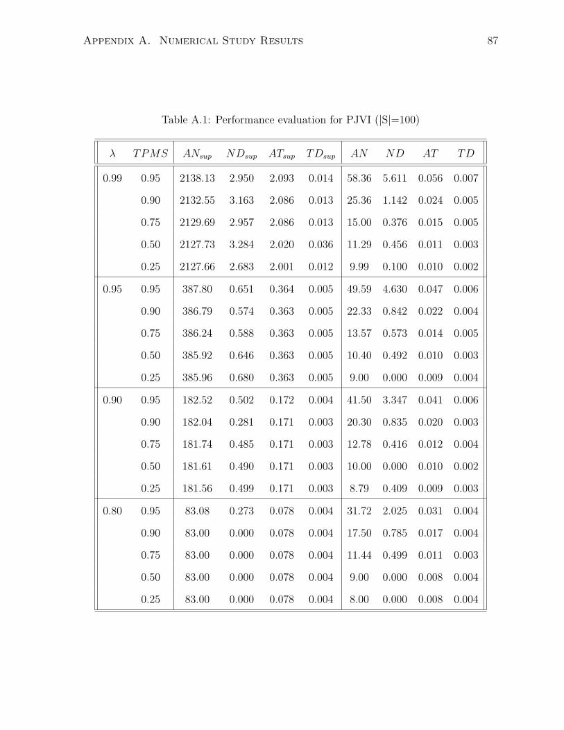
Appendix A. Numerical Study Results 87

Table A.1: Performance evaluation for PJVI (|S|=100)

λ TPMS ANsup NDsup ATsup TDsup AN ND AT TD

0.99 0.95 2138.13 2.950 2.093 0.014 58.36 5.611 0.056 0.007

0.90 2132.55 3.163 2.086 0.013 25.36 1.142 0.024 0.005

0.75 2129.69 2.957 2.086 0.013 15.00 0.376 0.015 0.005

0.50 2127.73 3.284 2.020 0.036 11.29 0.456 0.011 0.003

0.25 2127.66 2.683 2.001 0.012 9.99 0.100 0.010 0.002

0.95 0.95 387.80 0.651 0.364 0.005 49.59 4.630 0.047 0.006

0.90 386.79 0.574 0.363 0.005 22.33 0.842 0.022 0.004

0.75 386.24 0.588 0.363 0.005 13.57 0.573 0.014 0.005

0.50 385.92 0.646 0.363 0.005 10.40 0.492 0.010 0.003

0.25 385.96 0.680 0.363 0.005 9.00 0.000 0.009 0.004

0.90 0.95 182.52 0.502 0.172 0.004 41.50 3.347 0.041 0.006

0.90 182.04 0.281 0.171 0.003 20.30 0.835 0.020 0.003

0.75 181.74 0.485 0.171 0.003 12.78 0.416 0.012 0.004

0.50 181.61 0.490 0.171 0.003 10.00 0.000 0.010 0.002

0.25 181.56 0.499 0.171 0.003 8.79 0.409 0.009 0.003

0.80 0.95 83.08 0.273 0.078 0.004 31.72 2.025 0.031 0.004

0.90 83.00 0.000 0.078 0.004 17.50 0.785 0.017 0.004

0.75 83.00 0.000 0.078 0.004 11.44 0.499 0.011 0.003

0.50 83.00 0.000 0.078 0.004 9.00 0.000 0.008 0.004

0.25 83.00 0.000 0.078 0.004 8.00 0.000 0.008 0.004


Table A.2: Performance evaluation for JVI (|S|=100)


0.99 0.95 1697.210 24.781 1.668 0.026 1287.34 21.635 1.227 0.025

0.90 1924.030 9.481 1.890 0.015 1335.81 11.877 1.275 0.013

0.75 2048.300 4.541 2.015 0.014 1304.30 7.345 1.245 0.012

0.50 2087.070 4.312 1.988 0.036 1248.67 6.572 1.191 0.011

0.25 2100.510 2.922 1.983 0.011 1211.47 4.850 1.162 0.011

0.95 0.95 311.980 4.656 0.295 0.007 254.17 3.942 0.244 0.006

0.90 350.160 1.824 0.331 0.005 262.77 2.534 0.252 0.005

0.75 371.750 0.936 0.351 0.004 255.92 1.529 0.247 0.005

0.50 378.760 0.726 0.358 0.004 245.09 1.349 0.236 0.005

0.25 381.240 0.653 0.359 0.005 237.83 1.120 0.229 0.004

0.90 0.95 147.300 2.263 0.139 0.004 124.43 2.185 0.120 0.004

0.90 165.470 0.915 0.157 0.005 128.51 0.835 0.123 0.005

0.75 175.140 0.493 0.166 0.005 125.06 0.776 0.121 0.003

0.50 178.230 0.423 0.169 0.003 119.75 0.626 0.116 0.005

0.25 179.290 0.456 0.169 0.004 116.11 0.601 0.112 0.004

0.80 0.95 69.000 0.752 0.065 0.005 59.67 0.726 0.057 0.005

0.90 75.920 0.273 0.072 0.004 61.22 0.579 0.059 0.003

0.75 80.040 0.197 0.076 0.005 59.37 0.485 0.058 0.004

0.50 81.510 0.502 0.077 0.005 56.94 0.239 0.056 0.005

0.25 82.000 0.000 0.078 0.004 55.00 0.000 0.053 0.005


Table A.3: Performance evaluation for PGSVI (|S|=100)


0.99 0.95 1321.670 34.282 1.289 0.036 1056.51 28.732 1.001 0.030

0.90 1203.410 21.624 1.173 0.022 957.26 15.797 0.910 0.017

0.75 1140.640 11.147 1.113 0.013 904.90 8.304 0.859 0.011

0.50 1120.150 7.237 1.057 0.019 887.79 6.376 0.844 0.009

0.25 1114.180 4.558 1.042 0.008 882.04 3.869 0.844 0.009

0.95 0.95 242.190 6.356 0.226 0.008 210.00 4.971 0.201 0.007

0.90 221.700 3.786 0.207 0.006 190.85 2.595 0.181 0.004

0.75 209.840 2.242 0.196 0.005 179.53 1.800 0.172 0.005

0.50 206.240 1.256 0.194 0.005 175.67 1.035 0.168 0.004

0.25 204.960 0.887 0.191 0.003 174.73 0.863 0.167 0.005

0.90 0.95 116.670 2.089 0.109 0.004 103.40 2.184 0.099 0.005

0.90 106.100 1.784 0.099 0.004 94.02 1.484 0.090 0.004

0.75 100.090 0.889 0.093 0.005 88.83 0.711 0.085 0.005

0.50 98.380 0.632 0.092 0.004 86.79 0.537 0.084 0.005

0.25 97.810 0.486 0.091 0.003 86.24 0.429 0.083 0.005

0.80 0.95 54.560 1.140 0.051 0.003 50.89 1.004 0.049 0.004

0.90 50.110 0.875 0.047 0.005 45.76 0.653 0.044 0.005

0.75 47.280 0.451 0.043 0.005 43.05 0.435 0.042 0.004

0.50 46.520 0.502 0.044 0.005 42.42 0.496 0.041 0.002

0.25 46.050 0.219 0.043 0.004 42.00 0.000 0.041 0.003


Table A.4: Performance evaluation for GSVI (|S|=100)


0.99 0.95 868.030 32.084 0.852 0.033 715.57 27.258 0.682 0.028

0.90 987.580 21.044 0.970 0.022 796.98 15.284 0.761 0.016

0.75 1056.170 11.250 1.037 0.014 842.29 8.556 0.805 0.011

0.50 1078.040 7.203 1.027 0.020 856.57 6.315 0.819 0.010

0.25 1086.160 4.592 1.025 0.007 861.40 3.921 0.828 0.008

0.95 0.95 162.980 5.698 0.154 0.006 144.14 4.956 0.138 0.006

0.90 183.200 3.706 0.173 0.006 159.46 2.528 0.154 0.005

0.75 194.600 2.265 0.183 0.005 167.58 1.736 0.162 0.005

0.50 198.670 1.173 0.187 0.005 169.63 1.051 0.163 0.005

0.25 199.960 0.887 0.189 0.003 170.76 0.900 0.165 0.005

0.90 0.95 79.340 2.487 0.075 0.005 71.97 2.316 0.070 0.004

0.90 88.360 1.605 0.083 0.005 79.09 1.272 0.077 0.004

0.75 93.050 0.968 0.088 0.004 82.99 0.785 0.081 0.003

0.50 94.920 0.677 0.089 0.004 83.97 0.594 0.081 0.003

0.25 95.480 0.502 0.090 0.002 84.40 0.492 0.082 0.004

0.80 0.95 38.880 1.183 0.037 0.005 37.00 0.910 0.036 0.005

0.90 42.270 0.790 0.040 0.002 38.89 0.680 0.038 0.004

0.75 44.120 0.327 0.042 0.004 40.37 0.485 0.038 0.004

0.50 44.900 0.302 0.042 0.004 41.00 0.000 0.040 0.001

0.25 45.000 0.000 0.042 0.004 41.00 0.000 0.040 0.002


Table A.5: Performance evaluation for PAE and HAE1 (AN and AT)(|S|=100)

λ TPMS ANP NDP ATP TDP ANH1 NDH1 ATH1 TDH1

0.99 0.9 13.26 1.624 0.024 0.005 13.26 1.624 0.024 0.005

0.8 10.14 0.865 0.018 0.004 10.14 0.865 0.018 0.004

0.5 7.71 0.671 0.015 0.005 6.36 0.675 16.644 0.018

0.1 6.35 0.575 0.013 0.005 4.65 0.626 19.087 0.034

0.95 0.9 11.34 0.855 0.018 0.004 11.34 0.855 0.018 0.004

0.8 9.00 0.964 0.015 0.005 9.00 0.964 0.015 0.005

0.5 6.98 0.651 0.012 0.004 6.32 0.665 16.652 0.018

0.1 5.63 0.506 0.011 0.002 4.51 0.502 19.083 0.014

0.9 0.9 9.74 0.645 0.015 0.005 9.74 0.645 0.016 0.005

0.8 8.08 1.051 0.014 0.005 8.08 1.051 0.013 0.004

0.5 6.39 0.723 0.011 0.003 6.00 0.711 16.648 0.020

0.1 5.45 0.557 0.010 0.001 4.61 0.601 19.073 0.015

0.8 0.9 8.50 0.674 0.013 0.005 8.50 0.674 0.013 0.004

0.8 7.00 0.853 0.011 0.003 7.00 0.853 0.011 0.003

0.5 5.76 0.605 0.010 0.002 5.44 0.556 16.645 0.018

0.1 4.99 0.502 0.009 0.004 4.37 0.562 19.078 0.014


Table A.6: Performance evaluation for PAE, HAE2 and IAE (AN) (|S|=200)

λ TPMS ANP NDP ANH2 NDH2 ANI NDI

0.99 0.98 31.85 4.355 31.22 4.338 30.15 4.823

0.95 14.34 1.450 14.23 1.442 14.17 1.483

0.9 10.74 0.881 10.69 0.880 10.56 0.855

0.8 8.87 0.749 8.82 0.751 8.72 0.825

0.5 7.19 0.568 7.02 0.617 6.97 0.511

0.1 6.02 0.448 5.66 0.558 5.59 0.552

0.95 0.98 24.96 3.481 24.37 3.456 23.34 3.376

0.95 12.21 1.229 12.14 1.218 11.91 1.147

0.9 9.45 0.967 9.42 0.967 9.18 0.892

0.8 7.90 0.774 7.86 0.779 7.74 0.661

0.5 6.41 0.557 6.27 0.540 6.20 0.471

0.1 5.39 0.550 5.14 0.405 5.09 0.379

0.9 0.98 21.03 2.877 20.52 2.857 20.28 3.542

0.95 11.03 1.170 10.96 1.166 10.79 1.157

0.9 8.68 0.901 8.64 0.889 8.58 0.855

0.8 7.33 0.720 7.28 0.718 7.24 0.754

0.5 6.06 0.589 5.89 0.632 5.87 0.506

0.1 5.17 0.422 4.91 0.512 4.85 0.479

0.8 0.98 16.22 2.314 15.79 2.286 15.26 2.177

0.95 9.52 1.097 9.45 1.086 9.26 1.122

0.9 7.68 0.857 7.65 0.861 7.55 0.796

0.8 6.64 0.670 6.60 0.667 6.51 0.643

0.5 5.54 0.611 5.40 0.580 5.35 0.520

0.1 4.84 0.491 4.44 0.528 4.38 0.522


Table A.7: Performance evaluation for PAE, HAE2 and IAE (AT) (|S|=200)

λ TPMS ATP TDP ATH2 TDH2 ATI TDI

0.99 0.98 0.140 0.010 0.504 0.010 0.156 0.010

0.95 0.071 0.004 0.455 0.005 0.099 0.004

0.9 0.056 0.005 0.463 0.005 0.085 0.005

0.8 0.048 0.004 0.501 0.005 0.079 0.004

0.5 0.040 0.002 0.607 0.005 0.075 0.005

0.1 0.034 0.005 0.676 0.005 0.068 0.004

0.95 0.98 0.099 0.007 0.463 0.007 0.117 0.007

0.95 0.055 0.005 0.439 0.005 0.085 0.005

0.9 0.045 0.005 0.452 0.005 0.075 0.005

0.8 0.040 0.002 0.492 0.005 0.071 0.004

0.5 0.032 0.004 0.598 0.005 0.067 0.005

0.1 0.029 0.003 0.673 0.006 0.065 0.005

0.9 0.98 0.077 0.005 0.442 0.006 0.100 0.004

0.95 0.047 0.005 0.431 0.005 0.077 0.005

0.9 0.040 0.002 0.448 0.005 0.070 0.004

0.8 0.035 0.005 0.487 0.005 0.067 0.005

0.5 0.030 0.002 0.596 0.005 0.067 0.005

0.1 0.028 0.004 0.669 0.005 0.061 0.004

0.8 0.98 0.057 0.005 0.423 0.005 0.081 0.004

0.95 0.039 0.003 0.423 0.005 0.068 0.005

0.9 0.034 0.005 0.441 0.005 0.065 0.005

0.8 0.031 0.003 0.484 0.005 0.062 0.004

0.5 0.028 0.004 0.593 0.005 0.061 0.004

0.1 0.024 0.005 0.667 0.005 0.058 0.005


Table A.8: Performance evaluation for PAE and HAE (AN and AT)(|S|=200)

λ TPMS ANP NDP ATP TDP ANH NDH ATH TDH

0.99 0.98 31.32 4.35 0.515 0.011 22.36 3.88 0.117 0.007

0.95 14.20 1.37 0.462 0.006 10.41 1.34 0.081 0.004

0.9 10.73 0.90 0.471 0.006 8.03 0.93 0.073 0.005

0.8 8.84 0.73 0.507 0.006 6.72 0.71 0.069 0.004

0.5 7.06 0.63 0.614 0.006 5.42 0.61 0.067 0.005

0.1 5.68 0.55 0.685 0.006 4.39 0.52 0.063 0.005

0.95 0.98 24.49 3.58 0.472 0.008 20.05 3.49 0.108 0.007

0.95 12.07 1.31 0.446 0.006 9.96 1.29 0.079 0.005

0.9 9.43 0.95 0.459 0.006 7.85 0.94 0.072 0.005

0.8 7.83 0.72 0.499 0.006 6.61 0.73 0.068 0.005

0.5 6.30 0.57 0.606 0.006 5.36 0.57 0.066 0.005

0.1 5.14 0.39 0.681 0.006 4.32 0.49 0.063 0.005

0.9 0.98 20.73 2.92 0.452 0.007 18.03 2.86 0.100 0.006

0.95 10.97 1.19 0.438 0.006 9.55 1.18 0.076 0.005

0.9 8.71 0.94 0.454 0.006 7.62 0.95 0.070 0.004

0.8 7.32 0.69 0.493 0.006 6.45 0.71 0.066 0.005

0.5 5.92 0.57 0.604 0.006 5.23 0.53 0.065 0.005

0.1 4.90 0.49 0.677 0.006 4.28 0.48 0.063 0.005

0.8 0.98 15.68 2.06 0.431 0.006 14.33 2.04 0.087 0.005

0.95 9.33 1.08 0.429 0.006 8.57 1.07 0.071 0.004

0.9 7.67 0.85 0.448 0.005 7.07 0.84 0.066 0.005

0.8 6.63 0.73 0.490 0.005 6.14 0.73 0.063 0.005

0.5 5.40 0.57 0.599 0.006 5.05 0.54 0.063 0.005

0.1 4.46 0.54 0.668 0.005 4.20 0.44 0.061 0.003


Table A.9: Performance evaluation for PJVI, HTAE and MPAE1 (AN) (|S|=35937)

λ b AAPS AN1 ND1 AN2 ND2 AN3 ND3

0.97 1 8 567.17 3.43 567.17 3.43 567.17 3.43

27 567.42 3.71 567.42 3.71 567.42 3.71

125 567.91 3.92 567.91 3.92 567.91 3.92

0.97 2 8 567.92 3.33 567.92 3.33 567.92 3.33

27 567.14 3.52 567.14 3.52 567.14 3.52

125 566.84 3.86 566.84 3.86 566.84 3.86

0.97 3 8 567.31 3.86 567.31 3.86 567.31 3.86

27 567.47 3.85 567.47 3.85 567.47 3.85

125 567.35 3.47 567.35 3.47 567.35 3.47

0.97 4 8 567.90 3.42 567.90 3.42 567.90 3.42

27 567.33 3.49 567.33 3.49 567.33 3.49

125 567.16 3.50 567.16 3.50 567.16 3.50

0.95 1 8 331.34 1.84 331.34 1.84 331.34 1.84

27 331.46 2.04 331.46 2.04 331.46 2.04

125 331.55 1.90 331.55 1.90 331.55 1.90

0.95 2 8 331.48 1.97 331.48 1.97 331.48 1.97

27 331.55 2.02 331.55 2.02 331.55 2.02

125 331.25 2.16 331.25 2.16 331.25 2.16

0.95 3 8 331.68 1.85 331.68 1.85 331.68 1.85

27 331.33 1.92 331.33 1.92 331.33 1.92

125 331.88 2.08 331.88 2.08 331.88 2.08

0.95 4 8 331.13 1.99 331.13 1.99 331.13 1.99

27 331.41 2.17 331.41 2.17 331.41 2.17

125 331.41 1.66 331.41 1.66 331.41 1.66

0.9 1 8 156.84 0.87 156.84 0.87 156.84 0.87

27 156.73 0.91 156.73 0.91 156.73 0.91

125 156.76 0.88 156.76 0.88 156.76 0.88

0.9 2 8 156.85 0.87 156.85 0.87 156.85 0.87

27 156.87 0.79 156.87 0.79 156.87 0.79

125 156.68 0.80 156.68 0.80 156.68 0.80

0.9 3 8 156.92 0.81 156.92 0.81 156.92 0.81

27 156.89 0.86 156.89 0.86 156.89 0.86

125 156.90 0.88 156.90 0.88 156.90 0.88

0.9 4 8 156.75 0.85 156.75 0.85 156.75 0.85

27 156.93 0.88 156.93 0.88 156.93 0.88

125 156.88 0.92 156.88 0.92 156.88 0.92


Table A.10: Performance evaluation for PAE, P+HTAE and MPAE2 (AN) (|S|=35937)

λ b AAPS AN4 ND4 AN5 ND5 AN6 ND6

0.97 1 8 567.17 3.43 567.17 3.43 207.01 3.28

27 567.42 3.71 567.42 3.71 221.32 4.94

125 567.91 3.92 567.91 3.92 221.47 5.28

0.97 2 8 567.92 3.33 567.92 3.33 208.12 2.94

27 567.14 3.52 567.14 3.52 221.47 4.86

125 566.84 3.86 566.84 3.86 221.34 5.26

0.97 3 8 567.31 3.86 567.31 3.86 207.02 3.28

27 567.47 3.85 567.47 3.85 220.68 4.90

125 567.35 3.47 567.35 3.47 222.07 5.52

0.97 4 8 567.90 3.42 567.90 3.42 207.66 3.09

27 567.33 3.49 567.33 3.49 221.87 5.70

125 567.16 3.50 567.16 3.50 221.50 5.09

0.95 1 8 331.34 1.84 331.34 1.84 115.36 1.83

27 331.46 2.04 331.46 2.04 120.27 2.44

125 331.55 1.90 331.55 1.90 119.99 2.60

0.95 2 8 331.48 1.97 331.48 1.97 115.51 1.77

27 331.55 2.02 331.55 2.02 120.26 2.40

125 331.25 2.16 331.25 2.16 119.78 2.30

0.95 3 8 331.68 1.85 331.68 1.85 115.49 1.90

27 331.33 1.92 331.33 1.92 120.00 2.26

125 331.88 2.08 331.88 2.08 120.34 2.48

0.95 4 8 331.13 1.99 331.13 1.99 115.25 1.95

27 331.41 2.17 331.41 2.17 119.96 2.59

125 331.41 1.66 331.41 1.66 119.91 2.11

0.9 1 8 156.84 0.87 156.84 0.87 50.77 0.96

27 156.73 0.91 156.73 0.91 51.63 1.02

125 156.76 0.88 156.76 0.88 51.71 1.16

0.9 2 8 156.85 0.87 156.85 0.87 50.72 0.91

27 156.87 0.79 156.87 0.79 51.69 1.01

125 156.68 0.80 156.68 0.80 51.55 0.98

0.9 3 8 156.92 0.81 156.92 0.81 50.91 0.91

27 156.89 0.86 156.89 0.86 51.77 1.00

125 156.90 0.88 156.90 0.88 51.85 1.15

0.9 4 8 156.75 0.85 156.75 0.85 50.73 0.92

27 156.93 0.88 156.93 0.88 51.93 1.05

125 156.88 0.92 156.88 0.92 51.76 1.06


Table A.11: Performance evaluation for PJVI, HTAE and MPAE1 (AT ) (|S|=35937)

λ b AAPS AT1 TD1 AT2 TD2 AT3 TD3

0.97 1 8 23.52 2.29 18.08 0.28 20.84 0.19

27 65.86 2.24 44.30 0.44 32.91 0.45

125 227.10 1.57 183.40 1.27 70.70 0.51

0.97 2 8 23.57 0.25 18.02 0.36 20.75 0.28

27 61.85 1.15 43.20 0.28 28.89 0.19

125 226.67 1.54 183.10 1.25 48.86 0.33

0.97 3 8 23.52 0.26 18.02 0.35 20.64 0.30

27 61.86 1.16 43.20 0.30 27.54 0.21

125 226.78 1.38 183.27 1.13 45.06 0.28

0.97 4 8 23.54 0.25 18.03 0.36 22.34 0.31

27 61.84 1.17 43.18 0.28 28.97 0.20

125 226.83 1.41 183.19 1.13 45.95 0.29

0.95 1 8 13.73 0.15 10.52 0.19 12.76 0.19

27 36.15 0.66 25.23 0.16 19.26 0.15

125 132.57 0.76 107.12 0.62 41.28 0.24

0.95 2 8 13.74 0.16 10.53 0.20 12.11 0.18

27 36.16 0.67 25.25 0.16 16.89 0.11

125 132.25 0.89 107.06 0.71 28.55 0.18

0.95 3 8 13.75 0.15 10.54 0.19 12.08 0.18

27 36.13 0.69 25.23 0.16 16.09 0.11

125 132.67 0.84 107.23 0.68 26.39 0.28

0.95 4 8 13.73 0.15 10.52 0.20 13.03 0.19

27 36.14 0.72 25.24 0.16 16.93 0.14

125 132.31 0.74 107.10 0.53 26.86 0.14

0.9 1 8 6.50 0.08 4.99 0.09 6.05 0.08

27 17.10 0.33 11.94 0.08 9.10 0.07

125 62.66 0.36 50.67 0.28 19.52 0.12

0.9 2 8 6.50 0.08 4.99 0.10 5.73 0.08

27 17.11 0.31 11.96 0.07 7.99 0.06

125 62.64 0.32 50.64 0.26 13.51 0.07

0.9 3 8 6.50 0.08 4.99 0.10 5.72 0.10

27 17.11 0.32 11.96 0.08 7.62 0.05

125 62.71 0.36 50.72 0.29 12.46 0.08

0.9 4 8 6.49 0.07 4.98 0.10 6.17 0.09

27 17.12 0.32 11.96 0.09 8.02 0.06

125 62.69 0.37 50.71 0.30 12.71 0.08


Table A.12: Performance evaluation for PAE, P+HTAE and MPAE2 (AT ) (|S|=35937)

λ b AAPS AT4 TD4 AT5 TD5 AT6 TD6

0.97 1 8 22.78 0.30 24.24 0.13 10.12 0.21

27 48.70 0.93 42.00 0.70 16.98 0.41

125 141.34 1.87 118.26 1.55 34.24 0.82

0.97 2 8 22.80 0.17 24.25 0.27 10.19 0.15

27 45.81 0.42 40.29 0.31 16.90 0.37

125 140.87 1.84 117.91 1.52 34.19 0.81

0.97 3 8 22.75 0.22 24.23 0.27 10.41 0.17

27 45.97 0.49 40.36 0.36 17.08 0.38

125 141.19 1.64 118.18 1.36 34.63 0.85

0.97 4 8 22.78 0.21 24.26 0.25 11.34 0.17

27 45.99 0.45 40.37 0.35 18.20 0.47

125 141.01 1.62 118.04 1.35 35.56 0.81

0.95 1 8 13.16 0.11 14.14 0.15 5.81 0.11

27 26.33 0.27 23.31 0.21 9.29 0.19

125 80.19 0.95 66.89 0.85 18.55 0.40

0.95 2 8 13.17 0.13 14.15 0.15 5.66 0.10

27 26.35 0.26 23.30 0.20 9.18 0.18

125 80.07 0.94 66.78 0.81 18.52 0.35

0.95 3 8 13.19 0.12 14.16 0.16 5.80 0.11

27 26.32 0.24 23.28 0.19 9.30 0.18

125 80.33 0.92 67.02 0.80 18.78 0.39

0.95 4 8 13.16 0.13 14.13 0.15 6.29 0.11

27 26.32 0.28 23.29 0.22 9.85 0.21

125 80.15 0.77 66.85 0.68 19.26 0.34

0.9 1 8 6.16 1.91 6.69 0.07 2.56 0.05

27 12.08 0.12 10.82 0.09 3.98 0.09

125 36.17 0.44 30.22 0.41 8.00 0.18

0.9 2 8 6.14 1.71 6.69 0.07 2.48 0.05

27 12.10 0.11 10.83 0.09 3.95 0.08

125 36.11 0.37 30.16 0.34 7.98 0.15

0.9 3 8 6.13 1.81 6.69 0.07 2.56 0.05

27 12.10 0.12 10.84 0.09 4.01 0.08

125 36.24 0.44 30.29 0.39 8.10 0.18

0.9 4 8 6.07 1.64 6.68 0.08 2.77 0.05

27 12.11 0.12 10.84 0.10 4.26 0.09

125 36.22 0.43 30.26 0.38 8.32 0.18

Bibliography

[1] Abbad, M., and H. Boustique. A Decomposition Algorithm for Limiting Average

Markov Decision Problems. Operations Research Letters , 31:473–476, 2003.

[2] Amir, r., and A. Hadim. Some Structured Dynamic Programs Arising in Economics.

Computers Mathematical Applications, 24:209–218, 1992.

[3] Amir, r., and A. Hadim. Optimal Inventory Control Policy Subject to Different Selling

Prices of Perishable Commodities. International Journal of Production Economics ,

60:389–394, 1999.

[4] Anderson, R. J. Scheduled Maintenance Optimization System. Journal of Aircraft,

31:459–462, 1994.

[5] Bellman, R. E. Dynamic Programming. Princeton University Press, Princeton, NJ,

1957.

[6] Benjaafar, S., and M. Elhafsi. Production and Inventory Control of a Single Product

Assemble-To-Order System With Multiple Customer Classes. Management Science ,

52:1896–1912, 2006.

[7] Blackwell, D. Discounted Dynamic Programming. The Annals of Mathematical Statis-

tics, 36:226–235, 1965.

[8] Buchholz, P. Adaptive Aggregation/Disaggregation Algorithm for Hierarchical

Markovian Models. European Journal of Operational Research , 116:545–564, 1999.

99

Bibliography 100

[9] Chan, F. T. S., S. H. Chung, L. Y. Chan, G. Finke, and M. K. Tiwari. Solving

Distributed FMS Scheduling Problems Subject to Maintenance: Genetic Aalgorithms

Approach. Robotics and Computer-Integrated Manufacturing , 22:493–504, 2006.

[10] Chen, R.-R., and S. Meyn. Value Iteration and Optimization of Multiclass Queueing

Networks. Queueing Systems, 32:65–97, 1999.

[11] de Farias, D. P., and B. Van Roy. On Constraint Sampling in The Linear Program-

ming Approach to Approximate Dynamic Programming. Mathematics of Operations

Research, 29:462–478, 2004.

[12] Dembo, R. S., and M. Haviv. Truncated Policy Iteration Methods. Operations

Research Letters, 3:243–246, 1984.

[13] Demchenko, S. S., A. P. Knopov, and V. A pepelyaev. Optimal Strategies for

Inventory Control Systems with a Convex Cost Function. Cybernetics and Systems

Analysis , 36:891–897, 2000.

[14] Denardo, E. V. Contraction Mappings in The Theory Underlying Dynamic Pro-

gramming. SIAM Review, 9:165–177, 1967.

[15] Derman, C. Optimal Replacement and Maintenance Under Markovian Deterioration

With Probability Bounds on Failure. Management Science, 9:478–481, 1963.

[16] Derman, C. Finite State Markov Decision Processes, Academic Press, 1970.

[17] Even-Dar, E., S. Mannor and Y. Mansour. Action Elimination and Stopping Condi-

tions For The Mmulti-Armed Bandit and Reinforcement Learning Problems. Journal

of Machine Learning Research, 7:1079–1105, 2006.

[18] Fleischmann, M., and R. Kuik. On optimal Inventory Control With Independent

Stochastic Item Returns. European Journal of Operational Research , 151:25–37, 2003.

Bibliography 101

[19] Gosavi, A. Simulation-Based Optimization : Parametric Optimization Techniques

and Reinforcement Learning. Kluwer Academic Publishers, 2003.

[20] Grinold, R. C. Elimination of Supoptimal Actions in Markov Decision Problems.

Operations Research, 21:848–851, 1973.

[21] Hartley, R., A. C. Lavercombe and L. C. Thomas. Computational Comparison of

Policy Iteration Algorithms For Discounted Markov Decision Processes. Computers

and Operations Research, 13:411–420, 1986.

[22] Haskose, A., B. G. Kingsman, and D. Worthington. Modelling Flow and Jobbing

Shops as a Queueing Network for Workload Control. International Journal of Produc-

tion Economics , 78:271–285, 2002.

[23] Haskose, A., B. G. Kingsman, and D. Worthington. Performance Analysis of Make-

To-Order Manufacturing Systems Under Different Workload Control Regimes. Inter-

national Journal of Production Economics , 90:169–186, 2004.

[24] Hastings, N. A. J. and J. M. C. Mello. Tests For Suboptimal Actions in Discounted

Markov Programming. Management Science, 19:1019–1022, 1973.

[25] Hastings, N. A. J. Tests for Nonoptimal Actions in Undiscounted Finite Markov

Decision Chains. Management Science, 23:87–92, 1976.

[26] Haviv, M. Aggregation/Disaggrigation Methods For Computing the Stationary Dis-

tribution of Markov Chain. SIAM Journal on Numerical Analysis , 24:952–966, 1987.

[27] Haviv, M. On Censored Markov Chains, Best Augmentations and Aggrega-

tion/Disaggregation Procedures. Computers and Operations Research , 26:1125–1232,

1999.

Bibliography 102

[28] Herzberg, M., and U. Yechiali. Criteria For Selecting the Relaxation Factor of

The Value Iteration Algorithm For Undiscounted Markov and Semi-Markov Decision

Processes. Operations Research Letters, 10:193–202, 1991.

[29] Herzberg, M., and U. Yechiali. Accelerated Procedures of The Value Iteration Al-

gorithm For Discounted Markov Decision Processes, Based on One-Step Lookahead

Analysis. Operations Research, 42:940–946, 1994.

[30] Herzberg, M., and U. Yechiali. A K-Step Look-Ahead Analysis of Value Iteration

Algorithms For Markov Decision Processes. Europian jornal of Operations Research,

88:622–636, 1996.

[31] Heyman, D. P., and M. J. Sobel. Stochastic Models in Operations Research, Volume

II, New York: McGraw-Hill Book Company, 1984.

[32] Hipp, S. K., and U. D. Holzbaur. Decision Processes With Monotone Hysteretic

Policies. Operations Research , 36:585–588, 1988.

[33] Howard, R. Dynamic Programming and Markov Processes. J. Wiley, New York,

1960.

[34] Hubner, G. Improved Procedures For Eliminating Suboptimal Actions in Markov

Programming by The Use of Contraction Properties. in Transactions of the Seventh

Prague Conference of Information Theory, Statistical Decision Functions, Random

Processes, (D. Reidel, Dordrecht), pp. 257–263, 1977.

[35] Hubner, G. Bounds and Good Policies in Stationary Finit-Stage Markovian Decision

Problems. Advanced Applied Probability, 12:154-173, 1980.

[36] Jin, X., H. H. Tana, and J. Sun. A State-Space Partitioning Method Ffor Pricing

High-Dimensional American-Style Options. Mathematical Finance , 17:399–426, 2007.

Bibliography 103

[37] Kim, K. -E., and T. Dean. Solving Factored MDPs Using Non-Homogeneous Parti-

tions. Artificial Intelligence , 147:225–251, 2003.

[38] Kitaev, M. Yu., and R. F. Serfozo M/M/1 Queues With Switching Costs and Hys-

teretic Ooptimal Control. Operations Research, 47:310–312, 1999.

[39] Koehler, G. J. Bounds and Elimination in Generalized Markov Decisions. Naval

research logistics quarterly , 28:83–92, 1981.

[40] Kushner, H. J., and A. J. Kleinman Accelerated Procedures For The Solution of

Discrete Markov Control Problems. IEEE Transactions on Automatic Control, 16:147–

152, 1971.

[41] Kushner, H. J. Domain Decomposition For Large Markov Chain Controll Prob-

lems and NonLinear Elliptic-Type Equations. SIAM Journal of Scientific Computing,

18:1494–1516, 1997.

[42] Kuter, U., and J. Hu Computing and Using Lower and Upper Bounds For Action

Elimination in MDP Planning. Miguel and W. Ruml (Eds.): SARA 2007, LNAI 4612,

pp. 243U257, 2007.

[43] Lam, Y. Detecting Optimal and Non-Optimal Actions in Average-Cost Markov

Decision Processes. Microelectronics Reliability, 37:615–622, 1997.

[44] Lasserre, J. B. Detecting Optimal and Non-Optimal Actions in Average-Cost Markov

Decision Processes. Journal of Applied Probability , 31:979–990, 1994.

[45] Lee, I. S. K., and H. Y.K. Lau. Adaptive state space partitioning for reinforcement

learning. Engineering Applications of Artificial Intelligence, 17:577–288, 2004.

[46] Littman, M. L., J. Goldsmith, and M. Mundhenk. The Computational Complexity

of Probabilistic Planning. Journal of Artificial Intelligence Research , 9:1–36, 1998.

Bibliography 104

[47] Littman, M. L., T. L. Dean, and L. P. Kaelbling. A Survey of Computational

Complexity Results in Systems and Control. Automatica, 36:1249–1274, 2000.

[48] Lu, F. V., and R. F. Serfozo. M/M/1 Queueing Decision Processes With Monotone

Hysteretic Optimal Policies. Operations Research, 32:1116–1132, 1984.

[49] Luo, J., M. B. Friedman. A Study on Decomposition Methods. Computers Mathe-

matical Applications, 21:79-84, 1991.

[50] MacQueen, J. A Test For Suboptimal Actions in Markov Decision Problems. Oper-

ations Research, 15:559–561, 1967.

[51] Madras, N., and D. Randall. Markov Chain Decomposition For Convergence Rate

Analysis. OAnnals of Applied Probability , 12:581–606, 2002.

[52] Manne, A. S. Linear Programming and Sequential Decisions. Management Science,

6:259–267, 1960.

[53] Marek, I. Quasi-Birth-And-Death Processes, Level-Geometric Distributions. An Ag-

gregation/Disaggregation Approach. Journal of Computational and Applied Mathe-

matics , 152:277–288, 2003a.

[54] Marek, I., and P. Mayer. Convergence Theory of Some Classes of Iterative Ag-

gregation/Disaggregation Methods for Computing Stationary Probability Vectors of

Stochastic Matrices. Linear Algebra and Its Applications , 363:177–200, 2003b.

[55] Moustafa, M.S., E.Y. Abdel Maksoudb, and S. Sadekb. Optimal Major and Minimal

Maintenance Policies for Deteriorating Systems. Reliability Engineering and System

Safety, 83:363–368, 2004.

[56] Mrkaic, M. Policy Iteration Accelerated With Krylov Methods. Journal of Economic

Dynamics and Control, 26:517–545, 2002.

Bibliography 105

[57] Novoa, E. Simple Model-Based Exploration and Exploitation of Markov Decision

Processes Using the Elimination Algorithm. Lecture Notes in Computer Science (in-

cluding subseries Lecture Notes in Artificial Intelligence and Lecture Notes in Bioin-

formatics) , 4827 LNAI:327–336, 2007.

[58] Plum, H. J. Optimal Monotone Hysteretic Markov Policies in an M/M/1 Queueing

Model With Switching Costs and Finite Time Horizon. ZOR - Methods and Models of

Operations Research, 35:377–399, 1991.

[59] Ohno, K., and T. Ishigaki. A Multi-Item Continuouse Review Inventory System

With Compound Poisson Demands. Mathematical Methods of Operations Research,

53:147–165, 2001.

[60] Porteus, E. L. Some Bounds For Discounted Sequential Decision Processes. Man-

agement Science, 18:7–11, 1971.

[61] Porteus, E. L. Bounds and Transformations For Discounted Finite Markov Decision

Chains. Operations Research , 23:761–784, 1975.

[62] Porteus, E. L., and J. Totten Accelerated Computation of The Expected Discounted

Return in a Markov Chain. Operations Research , 26:350–358, 1978.

[63] Porteus, E. L. Computating The Discounted Return in Markov and Semi-Markov

Chains. Naval Research Logestics Quarterly, 28:567–578, 1981.

[64] Presman, E., S. Sethi, and Q. Zhang. Optimal Feedback Production Planning in a

Stochastic N-Machine Flowshop. Automatica, 31:1325–1332, 1995.

[65] Presman, E. L., S. P. Sethi, H. Zhang, and A. Bisi. Average Cost Optimal Policy

For a Stochastic Two-Machine Flowshop With Limited Work-In-Process. Nonlinear

Analysis, Theory, Methods and Applications ,47:5671-5678, 2001.

Bibliography 106

[66] Popyack, J. L., R. L. Brown, and C.C. White. Discrete Versions of an Algorithm

Due to Varaiya. IEEE Trans. Automat. Control, 24:503–504, 1979.

[67] Puterman, M. L., and M. C. Shin. Modified Policy Iteration Algorithms For Dis-

counted Markov Decision Problems. Management Science, 24:1127–1137, 1978.

[68] Puterman, M. L., and M. C. Shin. Action Elimination Procedures For Modified

Policy Iteration Algorithms. Operations Research, 30:301–318, 1982.

[69] Puterman, M. L. Markov Desision Processes: Discret Stochastic Dynamic Program-

ming, New York: Wiley, 1994.

[70] Ruszczynski, A Decomposition Methods in Stochastic Programming. Mathematical

Programming, 79:333-353, 1997.

[71] Sadjadi, D., and P. F. Bestwick. A Stagewise Action Elimination Algorithm For The

Discounted Semi-Markov Problem. The Journal of the Operational Research Society,

30:633–637, 1979. 1985.

[72] Schweitzer, P., and A. Seidmann. Generalized Polinomial Approximation in Marko-

vian Desision Processes. Operations Research, 27:616–620, 1979. 1985.

[73] Serfozo, R. F. Monotone Optimal Policies For Markov Descison Processes. Mathe-

matical Programming, 79:202–215, 1976.

[74] Serfozo, R. F. Optimal Control of Random Walks, Birth and Death Processes, and

Queues. Advances in Applied Probability, 13:61–83, 1981.

[75] Sethi, S. P., H. Zhang, and Q. Zhang. Optimal Production Rates in a Deterministic

Two-Product Manufacturing System. Optimal Control Applications and Methods ,

21:125–135, 2000.

Bibliography 107

[76] Tamura, N. Minimizing Submodular Function on a Lattice. IEICE Transactions on

Fundamentals of Electronics, Communications and Computer Sciences E90-A , 2:467–

473, 2007.

[77] Thomas, L. C., R. Hartley, and L. C. Thomas. Computational Comparesion of Value

Function Algorithms For Discounted Markov Decision Processes. Operations Research

Letters, 2:72–76, 1983.

[78] Topkis, D. M. Ordered Optimal Solutions. Ph.D. Dissertation, Stanford University,

Stanford, CA., U.S.A, 1968.

[79] Topkis, D. M. Minimizing Submodular Function on a Lattice. Operations Research,

26:305–321, 1978.

[80] Topkis, D. M. Supermodularity and Complementarity . Princeton University Press,

1998.

[81] Trick, M. A., and S. E. Zin. A Linear Programming Approach to Solving Stochastic

Dynamic Programs. Working paper, Carnegie Mellon University, 1993.

[82] Trick, M. A., and S. E. Zin. Spline Approximations to Value Functions: A Linear

Programming Approach . Macroeconomic Dynamics, 1:255–277, 1997.

[83] Umanita, V. Classification and Decomposition of Quantum Markov Semigroups.

Probability Theory and Related Fields , 134:603–623, 2006.

[84] Veatch, M. H., and L. M. Wein. Monotone Control of Queueing Networks. Queueing

Systems, 12:391–408, 1992.

[85] Weber, R. R., and S. Stidham. Optimal Control of Services Rates in Networks of

Queues. Advanced Applied Probability, 19:202–218, 1987.

[86] White, C. C., and D. J. White. Markov Decision Processes. European Journal of

Operational Research, 39:1–16, 1989.

Bibliography 108

[87] White, D.J. Isotone Optimal Policies For Structured Markov Decision Processes.

European Journal of Operational Research, 7:396–402, 1981.

[88] White, D.J. Markov desision Processes, New York: Wiley, 1994.

[89] White, D.J., and W. T. Scherer. The Convergence of Value Iteration in Dis-

counted Markov Decision Processes. Journal of Mathematical Analysis and Appli-

cations, 182:348–360, 1994.

[90] Wingate, D., and K. D. Seppi. Solving Large MDPs Quickly With Partitioned Value

Iteration. Journal of Machine Learning Research, 1:1–33, 2003.

[91] Wingate, D., and K. D. Seppi. Prioritization Methods For Accelerating MDP Solvers.

Journal of Machine Learning Research, 6:851–881, 2005.

[92] Yannopoulos, E., and A. S. Alfa. An Approximation Method For Queues in Series

With Blocking. Performance Evaluation, 20:373–390, 1994.

[93] Zobel, C. W., and W. T. Scherer. An Empirical Study of Policy Convergence in

Markov Decision Process Value Iteration. Computers and Operations Research, 32:127–

142, 2005.

Documents

Accelerating Successive Approximation Algorithm … Tandem Queueing System ... successive approximation, policy iteration, ... Introduction and Thesis Outline 3 2. Successive over