Accelerated Determination of ASR Susceptibility During … · Krzysztof J. Lesnicki, Jin-Yeon Kim, Kimberly E. Kurtis, and Laurence J. Jacobs 8. Performing Organization Report No

Accelerated Determination of ASRSusceptibility During Concrete Prism Testing Through Nonlinear ImpactResonance Ultrasonic Spectroscopy

PUBLICATION NO. FHWA-HRT-13-085 OCTOBER 2013

Research, Development, and TechnologyTurner-Fairbank Highway Research Center6300 Georgetown PikeMcLean, VA 22101-2296

FOREWORD

Accurate, reliable, and timely laboratory assessment of concrete mixtures—aggregates combined with cementitious materials—is a critical component in ensuring the durability of concrete infrastructure from the adverse effects of the alkali-silica reaction (ASR). Currently, the “Concrete Prism Test” (American Society of Testing and Materials (ASTM) C1293) is the most reliable standard test method for assessing the suitability of materials and materials combinations for resistance to damage by ASR. However, the main drawback of this method is the 1- to 2-year duration required for the test. This research study evaluates a new nonlinear acoustic technique for characterization of ASR damage in standard concrete prism specimens. Nonlinear impact resonance acoustic spectroscopy offers fast and reliable measurement of the material nonlinearity. Microstructural changes that occur as a result of ASR cause an increase in the measured nonlinearity, which can be used as a measure of the amount of ASR-induced damage. This study evaluates 10 concrete mix designs with varying ASR reactivity. Both standard expansion tests and nonlinearity measurements are performed on the specimens. This report presents the results of those tests to illustrate the utility of this new method as a complementary technique for damage assessment of laboratory concrete prisms specimens. This report is intended for those who assess aggregate reactivity by ASTM C1293 or ASTM C1260.

Jorge E. Pagán-Ortiz Director, Office of Infrastructure

Research and Development

Notice This document is disseminated under the sponsorship of the U.S. Department of Transportation in the interest of information exchange. The U.S. Government assumes no liability for its contents or use thereof. This report does not constitute a standard, specification, policy, or regulation.

The U.S. Government does not endorse products or manufacturers. Trade and manufacturers’ names appear in this report only because they are considered essential to the object of the document.

Quality Assurance Statement The Federal Highway Administration (FHWA) provides high-quality information to serve Government, industry, and the public in a manner that promotes public understanding. Standards and policies are used to ensure and maximize the quality, objectivity, utility, and integrity of its information. FHWA periodically reviews quality issues and adjusts its programs and processes to ensure continuous quality improvement.

TECHNICAL REPORT DOCUMENTATION PAGE

1. Report No. FHWA-HRT-13-085

2. Government Accession No.

3. Recipient’s Catalog No.

4. Title and Subtitle Accelerated Determination of ASR Susceptibility During Concrete Prism Testing Through Nonlinear Resonance Acoustic Spectroscopy

5. Report Date October 2013

6. Performing Organization Code:

7. Author(s) Krzysztof J. Lesnicki, Jin-Yeon Kim, Kimberly E. Kurtis, and Laurence J. Jacobs

8. Performing Organization Report No.

9. Performing Organization Name and Address Georgia Institute of Technology 790 Atlantic Drive Atlanta, George 50332-0355

10. Work Unit No.

11. Contract or Grant No. DTFH61-08-R-00010

12. Sponsoring Agency Name and Address Office of Infrastructure Research & Development Federal Highway Administration 6300 Georgetown Pike McLean, VA 22101-2296

13. Type of Report and Period Covered Interim Report July 2009–June 2012

14. Sponsoring Agency Code

15. Supplementary Notes The Contracting Officer’s Representatives are Y.P. Virmani, HRDI-60, and Fred Faridazar, HRDI-20. We are grateful to FHWA’s ASR Technical Working Group for its valuable comments in addition to providing suggestions throughout the performance period.

16. Abstract Accurate, reliable, and timely laboratory assessment of concrete mixtures—aggregates combined with cementitious materials—is a critical component in ensuring the durability of concrete infrastructure from the adverse effects of the alkali-silica reaction (ASR). Currently, the “Concrete Prism Test” (ASTM C1293) is the most reliable standard test method for assessing the suitability of materials and materials combinations for resistance to damage by ASR. However, the main drawback of this method is the 1- to 2-year duration required for the test. This research study evaluates a new nonlinear acoustic technique for characterization of ASR damage in standard concrete prism specimens. Nonlinear impact resonance acoustic spectroscopy offers a fast and reliable measurement of the material nonlinearity. Microstructural changes that occur as a result of ASR cause an increase in the measured nonlinearity, which can be used as a measure of the amount of ASR-induced damage. This study evaluates 10 concrete mix designs with varying ASR reactivity. Both standard expansion tests and nonlinearity measurements are performed on the specimens. This report presents the results of those tests to illustrate the utility of the new method as a complementary technique for damage assessment of laboratory concrete prisms specimens.

17. Key Words Nonlinear Acoustics, Vibration, Concrete, Alkali Silica Reaction, ASR

18. Distribution Statement No restrictions. This document is available to the public through the National Technical Information Service, Springfield, VA 22161.

19. Security Classif. (of this report) Unclassified

20. Security Classif. (of this page) Unclassified

21. No. of Pages

76 22. Price

Form DOT F 1700.7 (8-72) Reproduction of completed page authorized

ii

iii

TABLE OF CONTENTS

CHAPTER 1. INTRODUCTION ................................................................................................ 1

CHAPTER 2. THEORETICAL BACKGROUND FOR NONLINEAR ACOUSTICS ......... 3

CHAPTER 3. SAMPLE PREPARATION ................................................................................. 7 MIX DESIGNS .......................................................................................................................... 7 CONCRETE PRISM SAMPLES .......................................................................................... 11

CHAPTER 4. NONLINEAR MEASUREMENT TECHNIQUES ......................................... 13 NRUS TEST SETUP............................................................................................................... 13

NRUS Results ....................................................................................................................... 16 Limitations of NRUS ............................................................................................................ 19

NIRAS TEST SETUP ............................................................................................................. 20 Preliminary NIRAS Results .................................................................................................. 21 Validation of NIRAS Test Setup .......................................................................................... 26 Attachment Method for Accelerometer ................................................................................ 28 Robustness of NIRAS Test Setup ......................................................................................... 35 Validation of Linear Assumption .......................................................................................... 39

SETUP SUMMARY ................................................................................................................ 40

CHAPTER 5. PETROGRAPHIC METHODS ........................................................................ 41 PETROGRAPHIC SAMPLE PREPARATION .................................................................. 41 INTERPRETATION OF PETROGRAPHIC IMAGES ..................................................... 41

CHAPTER 6. RESULTS ............................................................................................................ 43 EXPANSION RESULTS ........................................................................................................ 43 NIRAS RESULTS ................................................................................................................... 45 CORED SAMPLE RESULTS ................................................................................................ 53 PETROGRAPHY TO COMPLEMENT NIRAS RESULTS .............................................. 54

CHAPTER 7. CONCLUSIONS AND RECOMMENDATIONS ........................................... 63 CONCLUSIONS ..................................................................................................................... 63 RECOMMENDATIONS FOR FURTHER RESEARCH ................................................... 64

REFERENCES ............................................................................................................................ 65

iv

LIST OF TABLES

Table 1. ASTM C1260 results for the aggregates examined ........................................................ 10 Table 2. Mix design matrix for NIRAS and ASTM C1293 concrete prisms ............................... 10 Table 3. Chemical analysis data for Type I cement ...................................................................... 11 Table 4. Mix designs and expansions for Jobe concrete prism samples used for comparison

between NRUS and NIRAS .............................................................................................. 13 Table 5. Summary of reactivity classifications based on AMBT, CPT, and NIRAS ................... 48

v

LIST OF FIGURES

Figure 1. Equation. Nonlinear stress–strain relationship ................................................................ 3 Figure 2. Equation. Relationship between frequency shift and strain amplitude ........................... 3 Figure 3. Equation. Relationship between the frequency shift, the scaled hysteresis parameter,

and the signal amplitude ..................................................................................................... 4 Figure 4. Equation. Relationship between change in damping and strain amplitude ..................... 4 Figure 5. Equation. Relationship between the change in damping and the signal amplitude ......... 4 Figure 6. Equation. Integral to calculate “cumulative” nonlinearity .............................................. 5 Figure 7. Equation. Approximation of integral to calculate”cumulative” nonlinearity using a

Riemann sum ...................................................................................................................... 5 Figure 8. Photo. Las Placitas gravel aggregate as received ............................................................ 8 Figure 9. Photo. Spratt limestone aggregate as received ................................................................ 8 Figure 10. Photo. Adairsville limestone (coarse) aggregate as received ........................................ 8 Figure 11. Photo. Adairsville limestone (fine) aggregate as received ............................................ 9 Figure 12. Photo. Alabama sand aggregate as received .................................................................. 9 Figure 13. Photo. Illinois gravel aggregate as received .................................................................. 9 Figure 14. Graph. ASTM C1293 expansions of concrete prisms used in prior project ................ 13 Figure 15. Illustration. NRUS setup schematic ............................................................................ 14 Figure 16. Photo. NRUS test setup ............................................................................................... 14 Figure 17. Equation. Linear resonance frequency ........................................................................ 15 Figure 18. Equation. First compressional resonance frequency ................................................... 15 Figure 19. Graph. FFT for ASR-01 sample using NRUS ............................................................. 17 Figure 20. Graph. FFT for ASR-02 sample using NRUS ............................................................. 17 Figure 21. Graph. FFT for ASR-06 sample using NRUS ............................................................. 18 Figure 22. Graph. Results of frequency sweep for ASR-01 (NRUS) ........................................... 18 Figure 23. Graph. Results of frequency sweep with increasing voltage (NRUS) for ASR-01,

ASR-02, and ASR-06........................................................................................................ 19 Figure 24. Graph. Frequency shift variation for ASR-02 sample using NRUS ........................... 20 Figure 25. Photo. NIRAS test setup .............................................................................................. 21 Figure 26. Illustration. NIRAS setup schematic ........................................................................... 21 Figure 27. Graph. Typical NIRAS signal in time and frequency domains ................................... 22 Figure 28. Graph. Frequency spectrum for recorded acceleration signal ..................................... 23 Figure 29. Graph. FFT for ASR-01 sample using NIRAS ........................................................... 23 Figure 30. Graph. Normalized frequency versus amplitude for ASR-01 sample (a linear fit

to the data produces results in a measured nonlinearity of 3.7831) .................................. 24 Figure 31. Graph. FFT for ASR-02 sample using NIRAS ........................................................... 24 Figure 32. Graph. FFT for ASR-06 sample using NIRAS ........................................................... 25 Figure 33. Graph. Normalized frequency shift versus amplitude for ASR-01, ASR-02, and

ASR-06 samples using NIRAS ......................................................................................... 25 Figure 34. Graph. FFT for aluminum sample ............................................................................... 26 Figure 35. Graph. Normalized frequency shift versus amplitude for aluminum sample .............. 26 Figure 36. Equation. Modulus of elasticity ................................................................................... 27 Figure 37. Equation. Correction factor for fundamental flexural mode ....................................... 27 Figure 38. Photo. Bracket used for casting accelerometer attachment ......................................... 29 Figure 39. Photo. Cast accelerometer attachment for Sample 1 ................................................... 29 Figure 40. Photo. Cast accelerometer attachment for Sample 2 ................................................... 30

vi

Figure 41. Photo. Cast accelerometer attachment for Sample 3 ................................................... 30 Figure 42. Graph. FFT and frequency shift in the frequency domain for Sample 1 at 23 days

of age ................................................................................................................................. 31 Figure 43. Graph. FFT and frequency shift in linear format for Sample 1 at 23 days of age ....... 31 Figure 44. Graph. FFT and frequency shift in the frequency domain for Sample 1 at 30 days


of age ................................................................................................................................. 33 Figure 47. FFT and frequency shift in linear format for Sample 1 at 65 days of age ................... 33 Figure 48. Graph. FFT and frequency shift in the frequency domain for Sample 2 at 65 days


of age ................................................................................................................................. 35 Figure 51: Graph. FFT and frequency shift in linear format for Sample 3 at 65 days of age ....... 35 Figure 52. Graph. Variability of NIRAS measurements ............................................................... 36 Figure 53. Illustration. Schematic showing tested positions ......................................................... 36 Figure 54. Graph. Variability for Position 1 ................................................................................. 37 Figure 55. Graph. Variability for Position 2 ................................................................................. 37 Figure 56. Graph. Variability for Position 3 ................................................................................. 38 Figure 57. Graph. Variability for Position 4 ................................................................................. 38 Figure 58. Graph. Variability for damaged sample (note difference in y-axis scale) .................. 39 Figure 59. Graph. Results for higher amplitude excitation for ASR-06 ....................................... 40 Figure 60. Graph. Results for higher amplitude excitation for Mix 4 reference stored at

ambient conditions ............................................................................................................ 40 Figure 61. Photo. Unpolished stained section ............................................................................... 42 Figure 62. Photo. Polished stained section ................................................................................... 42 Figure 63. Graph. ASTM C1293 expansion results up to 400 days ............................................. 44 Figure 64. Graph. ASTM C1293 expansion results up to 100 days ............................................. 44 Figure 65. Graph. ASTM C1293 expansion results up to 750 days for NR, MR, and SCM

mixes ................................................................................................................................. 45 Figure 66. Graph. Example of extraction of nonlinearity parameter for Mix 3 at 47 days .......... 46 Figure 67. Graph. NIRAS results up to 750 days ......................................................................... 47 Figure 68. Graph. NIRAS results up to 100 days ......................................................................... 47 Figure 69. Graph. NIRAS results for reference mixes.................................................................. 49 Figure 70. Graph. Nonlinearity comparison between reference and tested samples for

HR Mix 4 at 250 days ....................................................................................................... 49 Figure 71. Graph. Comparison between reference and tested samples for HR Mix 4 at

250 days in the frequency domain .................................................................................... 50 Figure 72. Graph. Cumulative nonlinearity .................................................................................. 52 Figure 73. Graph. Cumulative nonlinearity for NR and MR mixes ............................................. 52 Figure 74. Graph. Changes in linear resonance frequency ........................................................... 53 Figure 75. Graph. Nonlinear measurement results on I-75 core ................................................... 54 Figure 76. Graph. Nonlinear measurement results on HWY 316 core ......................................... 54 Figure 77. Photo. Petrographic image for Mix 2 at 1 day ............................................................. 55

vii

Figure 78. Photo. Petrographic image for Mix 2 at 9 days ........................................................... 56 Figure 79. Graph. Comparison of expansion and nonlinearity results for Mix 2 ......................... 56 Figure 80. Graph. Comparison of expansion and nonlinearity results for Mix 4 ......................... 57 Figure 81. Photo. Image 1 of recast Mix 4 at 12 days .................................................................. 58 Figure 82. Photo. Image 2 of recast Mix 4 at 12 days .................................................................. 58 Figure 83. Photo. Image 1 of recast Mix 4 at 26 days .................................................................. 58 Figure 84. Photo. Image 2 of recast Mix 4 at 26 days .................................................................. 59 Figure 85. Photo. Image 1 recast Mix 4 at 40 days ....................................................................... 59 Figure 86. Photo. Image 2 recast Mix 4 at 40 days ....................................................................... 59 Figure 87. Photo. Image 1 of recast Mix 4 at 54 days .................................................................. 60 Figure 88. Photo. Image 2 of recast Mix 4 at 54 days .................................................................. 60 Figure 89. Photo. Image 1 of recast Mix 4 at 62 days .................................................................. 60 Figure 90. Photo. Image 2 of recast Mix 4 at 62 days .................................................................. 61 Figure 91. Photo. Image 1 of recast Mix 7 at 218 days ................................................................ 61 Figure 92. Photo. Image 2 of recast Mix 7 at 218 days ................................................................ 62 Figure 93. Photo. Image 1 for recast reference Mix 7 at 218 days ............................................... 62 Figure 94. Photo. Image 2 for recast reference Mix 7 at 218 days ............................................... 62

viii

LIST OF ABBREVIATIONS AND SYMBOLS

Abbreviations AMBT Accelerated Mortar Bar Test ASR Alkali-Silica Reaction ASTM Refers to ASTM International (formerly American Society for Testing and

Materials) standards CPT Concrete Prism Test FA Fly Ash FFT Fast Fourier Transform GDOT Georgia Department of Transportation HR Moderately to Highly Reactive aggregates according to their ASR behavior HWY Highway I-XX I represents interstate, numbers following denote specific interstate kSA kiloSamples MR Potentially (or May be) Reactive aggregates according to their ASR behavior NDE Nondestructive Evaluation NDT Nondestructive Testing NEWS Nonlinear Elastic Wave Spectroscopy NIRAS Nonlinear Impact Resonance Acoustic Spectroscopy Nm Nanometer NR Non-Reactive aggregates according to their ASR behavior NRUS Nonlinear Resonance Ultrasound Spectroscopy NWMS Nonlinear Wave Modulation Spectroscopy SCM Supplementary Cementing Materials SD Standard Deviation SNR Signal-to-Noise Ratio UV Ultraviolet UV-C light Ultraviolet Radiation at 0.00001 inches (254 nanometers) Symbols Stress

0E Linear Elastic Modulus

Coefficient of Quadratic Anharmonicity Coefficient of Cubic Anharmonicity Strain Measure of the Material Hysteresis Strain Amplitude

Strain Rate

0f Linear Resonance Frequency

f Resonance Frequency at Increased Excitation Amplitude

1C Coefficient Proportional to Material Hysteresis A Signal Amplitude

ix

η Scaled Hysteresis Parameter

0 Linear Damping Rate

Damping Rate at Increased Excitation Amplitude 3C Coefficient Proportional to Material Hysteresis Ω Nonlinear Damping Parameter C Cumulative Nonlinearity t Time, Thickness L Specimen Thickness in Direction of Wave Propagation v Wave Speed

0t Time of Arrival at Receiving Transducer

E Young’s Modulus of Elasticity m Mass b Width L Length t Thickness

ff Fundamental Resonant Frequency of Bar in Flexure

1T Correction Factor for Fundamental Flexural Mode Poisson’s Ratio

1

CHAPTER 1. INTRODUCTION

Durability is a major concern for infrastructure throughout the United States, as well as the rest of the world. One form of deterioration that may affect concrete structures is the alkali-silica reaction (ASR). This reaction typically takes a long period of time to cause damage that is visually apparent or that affects the serviceability of the structure; however, prevention of the reaction is critical to ensuring a long service life. This issue is particularly relevant in regions where there is a reliance on marginal aggregate resources, where low-alkali cement and appropriate supplementary cementing materials (SCM) are not readily available, and where there is significant exposure to external alkali sources, such as deicing salts and chemicals. However, interest in prolonging service life, increasing cement alkali contents, increasing cement content in concrete (and hence increasing alkali contents in concrete), as well as regional exhaustion of nonreactive aggregate sources, have all resulted in an need for more rapid and reliable methods for assessment of the resistance of concrete mixtures to alkali-silica reaction. Hence, it is becoming increasingly important to be able to assess a specific combination of materials to ensure their long-term durability in the field.

The ASR occurs between reactive siliceous mineral components of some aggregates and the alkaline pore solution present in cement-based materials (where the surrounding environment may contribute additional alkali ions). The result is a gel that swells in the presence of sufficient amounts of moisture, leading to concrete expansion, cracking, increased permeability, and decreased mechanical strength and stiffness.(1,2) Concrete, a brittle material, is particularly susceptible to cracking as a result of swelling of the gel because of its low tensile strength as well as weaker interfacial zones at the cement and aggregate boundary.

Currently, ASR susceptibility is assessed through length change in the concrete or mortar specimens over time while subjected to accelerated conditions. In the United States, the most common standard procedures for this type of test are the “Concrete Prism Test” (CPT), described in ASTM International (ASTM, formerly American Society of Testing and Materials) C1293, and the “Accelerated Mortar Bar Test” (AMBT), described in ASTM C1260.(3,4) The AMBT is a considerably quicker test but it has not been proven reliable in all cases. Also, the aggregate must be crushed and sieved to a specified gradation for this test; therefore, the results may not reflect field performance of the uncrushed aggregate. The most accurate method, with respect to field performance, is the CPT.(5) To evaluate aggregate reactivity, the test duration is 1 year; to evaluate mitigation measures, the duration is 2 years. Expansion of concrete prisms stored over water at 100 oF (38 oC) is monitored, with expansion of greater than 0.04 percent by the end of the test indicative of alkali reactivity. The prisms should be prepared using cement with total equivalent alkali content (Na2Oe) of 0.9±0.1 percent, with additional alkali added to the mix water to bring the total equivalent alkali content to 1.25 percent by mass of cementitious materials. The additional internal source of alkali and the elevated temperature are intended to accelerate the reaction while maintaining good correlation with field performance.

One issue with the test is the long test duration, which is viewed as a significant drawback.(5) Another drawback of the test is the use of the final expansion measurement as the sole measure of reactivity. For example, it can be difficult to interpret the potential of concrete mixtures for reactivity in the field, especially for CPT results close to the expansion limit of 0.04 percent. A direct measurement of damage would be an improvement. While there have been attempts to

2

relate the degree of reaction to expansion, there remains significant discussion centered on the designation of appropriate expansion limits as well as the appropriate duration of laboratory testing, particularly for AMBT, to define aggregate reactivity.(6) This further suggests that more accuracy in the screening of aggregate for ASR is necessary.

Flaws in materials, including microcracking and interfacial debonding, increase the material’s nonlinearity, which can be detected by nondestructive evaluation (NDE) techniques. In addition, the changes in nonlinear elastic properties are generally orders of magnitude greater than the changes in linear elastic properties.(7) Because the changes in nonlinear properties are more pronounced, there is an opportunity for earlier, as well as more accurate, damage detection using NDE techniques. Measurement of the nonlinear behavior can be accomplished using several different techniques, such as nonlinear wave modulation spectroscopy (NWMS), second harmonic generation, nonlinear resonance ultrasound spectroscopy (NRUS), and the technique that has been developed by the present investigators—the nonlinear impact resonance acoustic spectroscopy (NIRAS).(8,9) NRUS uses the thickness resonance of a longitudinal ultrasonic wave, and its accuracy depends on exciting this single frequency, which is in the ultrasonic range. In contrast, NIRAS excites structural resonances and depends on the cross-sectional area, length, and boundary conditions. These resonant peaks are relatively easy to excite and can be well spaced, depending on specimen geometry. Finally, NWMS uses multiple acoustic inputs to create a modulated signal and measures changes in these modulated signals. Of these, researchers have already applied NRUS to concrete samples with thermal damage, reinforced concrete beams, bone with mechanical damage, and slate with mechanical damage. (See References 10–13.) With regard to ASR damage, NWMS techniques have been applied to AMBT specimens and have shown potential for earlier detection of damage.(14,15) Originally, the group planned to use the NRUS technique, but the results showed inconsistencies for this prismatic sample geometry; hence, NIRAS is used for assessment of ASR damage in CPT samples because of the simplicity of the setup and the consistency and clarity of the results.

The NIRAS technique is based on the same basic principles as NRUS. Damaged specimens exhibit nonlinear behavior that is reflected in a decrease in resonance frequency with an increase in the level of excitation.(9,13) For low levels of strain excitation, researchers have shown that there is a linear relationship between the relative frequency shift and the excitation amplitude.(13) Because hysteresis effects are dominant in microcracked materials, the ratio of the relative frequency shift to excitation amplitude can be taken as a parameter proportional to one of the nonlinear elastic properties of materials, called the nonlinear hysteresis strength.(13) This hysteresis strength increases with accumulated damage and can be used as a quantitative measure of ASR damage.

The aim of the current research is to develop NIRAS as a reliable, nonlinear ultrasonic measurement technique that can more quickly quantify damage associated with ASR in concrete specimens. The results of these measurements of nonlinearity in concrete prisms undergoing ASR are compared with expansion. In addition, the research focuses on developing an understanding of the sensitivity of the technique as well as the reaction through petrographic analysis. This report describes the NIRAS technique that has been developed for quantifying ASR damage in concrete prisms subjected to standard accelerated laboratory test conditions.

3

CHAPTER 2. THEORETICAL BACKGROUND FOR NONLINEAR ACOUSTICS

It is well known that cracks within a material decrease its resonance frequency by decreasing the overall stiffness of the structure. In addition to this linear change in frequency, researchers have demonstrated that cracks are also responsible for nonlinear effects, including the strain amplitude dependent resonance frequency shift.(16,17) Microcracks inside a material form a network that acts as a nonlinear bond system. The nonlinear behavior of this bond system can be attributed to Hertzian contact of crack faces and/or opening and closing of cracks in response to wave motion. Using the phenomenological model for hysteresis and classical nonlinear constitutive relationships, researchers have shown that the nonlinear stress–strain relationship can be shown as the equation in figure 1.(9,13).

sgn1 20 E

Figure 1. Equation. Nonlinear stress–strain relationship

where

= stress, 2m

N

0E = linear elastic modulus, 2m

N

= coefficient of quadratic anharmonicity = coefficient of cubic anharmonicity

= strainL

L, where L is length

= measure of the material hysteresis = strain amplitude

= strain rate, second

1)sgn( if 0 , -1 if 0 , and 0 if 0 Assuming that effects of hysteresis are dominant in microcracked materials, the relationship between frequency shift and strain amplitude shown in figure 2 is valid for low levels of strain excitation.(13)

10

0 Cf

ff

Figure 2. Equation. Relationship between frequency shift and strain amplitude

where

0f = linear resonance frequency, Hz

f = resonance frequency at increased excitation amplitude, Hz

4

1C = coefficient proportional to material hysteresis At higher amplitudes, there will also be an additional quadratic term for the strain amplitude

21 D ; however, because the experiments are performed at low levels of strain excitation, this

higher-order term can be ignored. In these experiments, the amplitude of the signal, A , which is proportional to the strain amplitude, , is measured instead of the strain amplitude. As a result, the absolute hysteresis parameter, , is not measured. Instead, a scaled hysteresis parameter proportional to is used as a measure of the material’s nonlinearity. The relationship used in this investigation is given by the equation shown in figure 3.

Af

ff

0

0

Figure 3. Equation. Relationship between the frequency shift, the scaled hysteresis parameter, and the signal amplitude

Chapter 4 explains in detail the extraction of the parameter from recorded data. An additional effect observed for hysteretic materials is the increase in damping for the sample. The equation in figure 4 shows that a linear relationship exists between the change in damping and the strain amplitude.(13)

30

0 C

Figure 4. Equation. Relationship between change in damping and strain amplitude

where

0 = linear damping rate

= damping rate at increased excitation amplitude

3C = coefficient proportional to material hysteresis

Because the signal amplitude is proportional to strain amplitude, the relationship between the change in damping and the signal amplitude is the equation shown in figure 5:

A

0

0

Figure 5. Equation. Relationship between the change in damping and the signal amplitude

where is termed the nonlinear damping parameter.

Because the nonlinearity is attributed to nonlinear interaction of cracks, relatively large and open cracks will not contribute to nonlinearity. Under this assumption, the nonlinearity parameter can be thought of as an “instantaneous” measure of nonlinearity. Because the measurements for

5

tracking nonlinearity in CPT samples are taken at rather long intervals of time, the “cumulative” nonlinearity C can be measured by integration, as shown in the equation in figure 6.

t

C d0

)(

Figure 6. Equation. Integral to calculate “cumulative” nonlinearity

With experimental data, a Riemann sum can be used to approximate this integral (see figure 7).

N

iiiiiC tttt

211 ))()()((

2

1

Figure 7. Equation. Approximation of integral to calculate”cumulative” nonlinearity using a Riemann sum

7

CHAPTER 3. SAMPLE PREPARATION

MIX DESIGNS

For this study, the researchers chose aggregate sources that would provide a range of alkali reactivity for assessment using the NIRAS technique. The aggregate sources were selected after discussion with the teams at Clemson University and University of Texas at Austin, as well as with input from members of Federal Highway Administration’s Technical Working Group on ASR. Some of the same aggregate sources were examined by while maintaining a range of alkali reactivity.

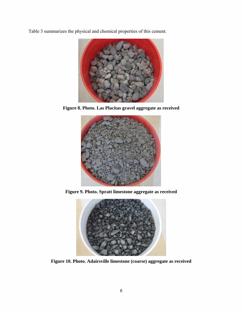
The reactivity of the aggregates, shown in their “as received” condition in figure 8, figure 9, figure 10 through figure 13, was initially assessed by AMBT. Each of the aggregates was crushed, when necessary, to fit the grading requirements prescribed in ASTM C1260. The dimensions of mortar bars created were 1 by 1 by 11.25 inch(es) (25 by 25 by 285 mm). For each mix design, three samples were created. The samples were cured at about 100-percent relative humidity and 73.4 °F (23 °C) for 24 hours. After demolding, the samples were cured for an additional 24 hours while immersed in tap water at 176 °F (80 °C). The initial length measurements were performed after this curing period. ASR was then induced in the mortar bars by immersing them in a 1N sodium hydroxide (NaOH) solution at 176 °F (80 °C). The samples were removed from the NaOH solution at regular intervals for expansion measurements as prescribed by ASTM C1260.

Table 1 presents the average expansion of the three samples at 14 days. Again, these results were used as an initial means for assessing the reactivity of the individual aggregates used in the concrete prisms. According to ASTM C1260, expansion at the end of the test that is less than 0.10 percent indicates innocuous behavior, expansion greater than 0.20 percent indicates potentially deleterious expansion, and expansion between 0.10 and 0.20 percent may be innocuous or deleterious in field behavior.

In this research, all specimens for evaluation by NIRAS and CPT were cast according to the ASTM C1293 standard. The mix design matrix, described in table 2, was developed to examine a range of ASR behavior, including the combination of two non-reactive aggregates (Mix 1), and the use of aggregates termed here as “moderately to highly reactive” (HR) and “potentially (or may be) reactive” (MR) aggregates, each in combination with the same non-reactive aggregate (NR). (The nonreactive aggregate used in all the mix designs is a limestone from Adairsville, GA.) Considering the ASTM C1260 results, along with historical aggregate standard test results and field performance history of these aggregates, each of the aggregates was preliminarily classified as NR, MR, or HR. Table 2 gives these classifications, along with other details about the concrete prism mixtures, including the sample naming scheme.

In addition, an ASTM C150 Type I cement with alkali equivalent of 0.88 percent, meeting the ASTM C1293 requirements, was used in the casting of CPT samples; the alkali content of the concrete was “boosted” to 1.25 percent by mass cementitious materials, in accordance with the standard.

8

Table 3 summarizes the physical and chemical properties of this cement.

Figure 8. Photo. Las Placitas gravel aggregate as received

Figure 9. Photo. Spratt limestone aggregate as received

Figure 10. Photo. Adairsville limestone (coarse) aggregate as received

9

Figure 11. Photo. Adairsville limestone (fine) aggregate as received

Figure 12. Photo. Alabama sand aggregate as received

Figure 13. Photo. Illinois gravel aggregate as received

10

Table 1. ASTM C1260 results for the aggregates examined

Aggregate Source 14-day AMBT

Expansion (percent) AMBT Classification

Limestone, GA 0.0787 Innocuous

Las Placitas, NM gravel 0.8533 Potentially deleterious

Spratt limestone, Canada (crushed)

0.2661 Potentially deleterious

Alabama sand, AL 0.1555 Innocuous or potentially deleterious

Central Illinois sand, IL 0.2088 Potentially deleterious

Table 2. Mix design matrix for NIRAS and ASTM C1293 concrete prisms

Mix ID Coarse Aggregate Fine Aggregate

Supplementary Cementing Materials

Mix 1 NR/NR Limestone, GA Limestone, GA —

Mix 2 HR/NR Las Placitas, NM gravel Limestone, GA —

Mix 3 NR/HR Limestone, GA Las Placitas, NM gravel

(crushed) —

Mix 4 HR/NR Spratt limestone,

Canada Limestone, GA —

Mix 5 NR/HR Limestone, GA Spratt limestone, Canada

(crushed) —

Mix 6 NR/MR Limestone, GA Alabama sand, AL —

Mix 7 NR/MR Limestone, GA Central Illinois Sand, IL —

Mix 8 HR/NR—25% FA Spratt limestone,

Canada Limestone, GA 25% Class F FA

Mix 9 NR/HR—25% FA Limestone, GA Spratt limestone, Canada(crushed)

25% Class F FA

Mix 10 NR/HR—25% FA Las Placitas, NM gravel Limestone, GA 25% Class F FA

NR = nonreactive MR = potentially or “may be” reactive HR = moderately to highly reactive FA = fly ash — = no supplementary cementing materials

11

Table 3. Chemical analysis data for Type I cement

Chemical Requirements ASTM C114

Test Result, (percent by mass)

Specification Limits Type 1

ASTM C150 (percentage by mass)

Silicon Dioxide (SiO2) 19.11 — Aluminum Oxide (Al2O3) 4.99 — Ferric Oxide (Fe2O3) 3.55 — Calcium Oxide (CaO) 60.66 — Magnesium Oxide (MgO) 3.24 — Sulfur Trioxide (SO3) 3.96 3.0 maximum Ignition Loss 2.71 3.0 maximum Insoluble Residue 0.24 0.75 maximum Carbon Dioxide—CO2 Percentage 1.71 — Limestone Percentage 4.1 5 maximum CaCO3 Percentage in Limestone 94.5 70 minimum Tricalcium Silicate (C3S) 42.9 — Tricalcium Aluminate (C3A) 7.0 < 8 C3S + 4.75C3A 76 100 maximum Equivalent Alkalis (Na2O+.658K2O) 0.88 — Chloride (Cl) 0.01 —

— No specification CONCRETE PRISM SAMPLES

All CPT samples were prepared using the ASTM C1293 testing procedure. Each sample, with a water-to-cement ratio of 0.45, is 3 inches long with a 3-inch square cross section (76 by 76 by 285 mm). The gradation for coarse aggregate was as specified in ASTM C1293. For fine aggregates, the gradation was adjusted through sieving or crushing to achieve a fineness modulus of 2.71. This was done to minimize any variability in NIRAS and expansion measurements that may have arisen owing to differences in fine aggregate gradation. For each mix design, eight specimens were cast, six with studs for expansion measurements and two without studs for petrographic examination. The samples were initially cured for 24 hours in a moist environment for 23.5 0.5 hours. After demolding, the initial lengths of three samples were recorded. Subsequently, those samples, along with one sample for petrography, were transferred to a container that is kept at 100.4 °F (38 °C) in an environmental chamber. The container also allows the elevation of the specimens above water, providing high relative humidity, which is necessary for inducing ASR. The remaining specimens were kept for reference at room temperature; when examined, these samples of the same composition as mixes 1 through 10 (table 2) but stored at ambient conditions are hereafter referred to as “reference” samples.

13

CHAPTER 4. NONLINEAR MEASUREMENT TECHNIQUES

Two nonlinear acoustic test setups—NRUS and NIRAS—were developed and compared with one another, using an existing set of concrete prism samples (ASR-01, ASR-02, and ASR-03) that had experienced varying amounts of expansion (see figure 14). The following sections describe the setups for NRUS and NIRAS. The three existing concrete prism samples examined using these methods had been subjected to 2 years of ASTM C1293 testing and subsequently stored for approximately 1 year at ambient conditions. All of these concrete samples contained a reactive sand from El Paso, TX (Jobe) but with different binder compositions. Figure 14, the expansion plot, shows expansions at the end of the 2-year test, but prior to storage in the laboratory. Table 4 shows the binder compositions for these three mixtures, along with the expansion measured after 2 years of testing.

Figure 14. Graph. ASTM C1293 expansions of concrete prisms used in prior project

Table 4. Mix designs and expansions for Jobe concrete prism samples used for comparison between NRUS and NIRAS

Sample Mix DesignASTM C1293

2-Year Expansion (percent) ASR-01 No SCMs 0.543ASR-02 8% metakaolin 0.048ASR-03 25% Class C FA 0.347

NRUS TEST SETUP

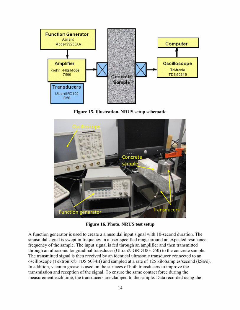
The original proposal considered using the NRUS method, and the initial set of measurements used the NRUS method for nonlinear parameter measurements. Figure 15 shows a representative schematic of the NRUS test setup, and figure 16 shows the physical test setup.

14

Figure 15. Illustration. NRUS setup schematic

Concretesample

Function generator

Oscilloscope

Transducers

Figure 16. Photo. NRUS test setup

A function generator is used to create a sinusoidal input signal with 10-second duration. The sinusoidal signal is swept in frequency in a user-specified range around an expected resonance frequency of the sample. The input signal is fed through an amplifier and then transmitted through an ultrasonic longitudinal transducer (Ultran® GRD100-D50) to the concrete sample. The transmitted signal is then received by an identical ultrasonic transducer connected to an oscilloscope (Tektronix® TDS 5034B) and sampled at a rate of 125 kiloSamples/second (kSa/s). In addition, vacuum grease is used on the surfaces of both transducers to improve the transmission and reception of the signal. To ensure the same contact force during the measurement each time, the transducers are clamped to the sample. Data recorded using the

15

oscilloscope is then analyzed using a developed analysis code, based on the software package Matlab®, on a computer.

With this setup, the first compressional wave resonance mode is excited, which can be calculated using the measured compressional wave speed (or the time of flight). The time of flight can be measured using a single transducer that sends a compressional wave through the thickness of the specimen. The time it takes for the signal to travel to the specimen boundary and reflect back to the source is the time of flight, t . Assuming a free surface boundary, the equation in figure 17 gives the linear resonance frequency.

tL

vf

2

1

20

Figure 17. Equation. Linear resonance frequency

where

L = specimen thickness in direction of wave propagation, meters

v = wave speed, s

m

t = time of flight, seconds However, because of the attenuation in the relatively large CPT specimens, there is no clear reflection of the source wave. Alternatively, two transducers are employed, and the time of arrival of the signal at the receiving transmitter is used to measure the first compressional resonance frequency, as shown in the equation in figure 18.

0

0

1

tL

vf

Figure 18. Equation. First compressional resonance frequency

where 0t = time of arrival at receiving transducer, seconds

Using the time of arrival, the resonance frequency was determined to be about 23 to 25 kilocycles per second (23 to 35 kHz), but when the frequency sweep was performed in this range, there was no clear peak in signal amplitude as expected for resonance. Therefore, the frequency was progressively increased until a significant increase in signal amplitude was detected. In other words, a sinusoid at a constant amplitude (voltage) and frequency was used as an input, and the amplitude of the transmitted signal was monitored as the input frequency was increased. The frequency at the observed amplitude increase was assumed to correspond to the first compressional resonance mode. The frequency sweep was then set to the range around this frequency, and the input voltage was progressively increased from about 10 to 190 volts. (All the measured data fall in this range but the same voltages are not used for different specimens.) The signal in the time domain was then analyzed with a fast Fourier transform (FFT) to obtain the frequency spectrum.

16

NRUS Results

The results of the FFT analysis for ASR-01, ASR-02, and ASR-06 are shown in figure 19, figure 20, and figure 21, respectively. The amplitude in the frequency domain is representative of the input signal amplitude, in volts, at a given frequency. The frequency at which the largest amplitude magnitude is measured (“output”), when applying a voltage varying from 10 to 190 volts, is then assumed to be the resonance frequency. The resonance frequency at the lowest excitation is assumed to be the linear resonance frequency, 0f . The left side of the equation

shown in figure 3 is then calculated by taking the difference between the linear resonance frequency and the frequency at the current excitation level, ff 0 , as shown in figure 19.

Further details can be found in Reference 10.

The calculated difference, ff 0 , is then normalized by the linear resonance frequency and

plotted against amplitude, as shown in figure 22. The nonlinear parameter, , is then the slope of the data as dictated by the equation in figure 3 and illustrated in figure 22.

Figure 23 presents the results for the three specimens tested together, along with the expansion recorded at 720 days and measured nonlinearity. Using the nonlinear parameter, each sample is clearly differentiated, showing distinguishable nonlinearity levels. Surprisingly, comparing NRUS results with the expansion values last recorded at 720 days, there is a discrepancy. The ASR-01 sample had more expansion at 720 days compared with ASR-06 but the measured ASR-06 nonlinearity is higher.

However, it is important to consider that the expansion results were not obtained at the same time as the nonlinearity measurements. Even though both ASR-01 and ASR-06 were well beyond the 0.04-percent expansion limit at 2 years of CPT, it is not clear how any further development of damage has progressed in the samples over this last year of ambient storage. Therefore, a comparison of expansion values from the end of the CPT test with nonlinearity measured by NRUS may not be valid.

17

Figure 19. Graph. FFT for ASR-01 sample using NRUS


18


Figure 22. Graph. Results of frequency sweep for ASR-01 (NRUS)

19

Figure 23. Graph. Results of frequency sweep with increasing voltage (NRUS) for ASR-01, ASR-02, and ASR-06

Limitations of NRUS

While the NRUS method distinguished between the different concrete mixtures, the peak assumed to be a resonance mode had a higher frequency than expected based on time of flight measurements. This local peak could not be confirmed to correspond to resonance frequencies or their harmonics. Because it is unclear where this local peak in the frequency domain originated, there is a question of robustness and reliability of the technique. In addition, there were difficulties with consistency in the measurements, as illustrated in figure 24. Measurements for the ASR-02 sample were repeated by reassembling the setup between measurements. Between each measurement trial, the transducers were removed from the specimen, the specimen and transducers were cleaned, and the specimen was again coupled to the transducers using vacuum grease. It was found that the results were not consistent when the setup was reassembled, producing considerable scatter. It is speculated that this could result from changes in the boundary (transducer to sample coupling) conditions caused by reassembling the test setup.

20

Figure 24. Graph. Frequency shift variation for ASR-02 sample using NRUS

NIRAS TEST SETUP

Because of inconsistent results obtained with the NRUS technique, an alternate method of excitation was attempted. The new technique uses the natural vibration of the specimen as the probing signal and is termed NIRAS, first introduced for assessment of alkali reactivity of aggregates by Chen et al.(9) Instead of using a frequency sweep employing transducers in ultrasonic frequency range, the sample is excited with a low amplitude impact. The setup is similar to the ASTM C215 procedure for the measurement of the transverse resonance frequency.(18) The specimen is placed on a 1.5-inch (38 mm) thick support mat to allow free vibration. A 5-oz. (140-g) hammer is used to strike the sample in the center of the specimen, as shown in figure 25. An accelerometer (PCB 353B13) is attached using super glue to one end of the specimen, at the center, where the response is at a maximum for the transverse mode. The sample is tested 1 minute after the attachment of the accelerometer, and the signal is then captured using a Tektronix™ TDS5034B oscilloscope and analyzed using Matlab®. The schematic for this setup is shown in figure 26. The signal duration captured by the oscilloscope is 0.4 seconds, which allows a complete decay of the response signal, with a sampling rate of 500 kSa/s. The signal is then “zero-padded” and analyzed in Matlab® using the FFT. The “zero-padding” increases the signal duration by appending trailing zeros at the end of the signal. This increases the apparent resolution in the frequency domain, allowing more accurate identification of the resonance peak frequency. The signal processing for both the NRUS and NIRAS techniques is essentially the same, and both rely on the same nonlinear resonance theory. However, as is demonstrated throughout this chapter, the NIRAS technique proves to be much more repeatable and robust.

21

Figure 25. Photo. NIRAS test setup

Figure 26. Illustration. NIRAS setup schematic

Preliminary NIRAS Results

The NIRAS technique was also initially applied to the Jobe aggregate concrete prism samples (see table 4) to assess the performance of the technique. The impact excites the specimen’s

22

natural vibration. Figure 27 shows the typical signal captured by the accelerometer in both the time and frequency domains (for ASR-01 in this case). Notice that the signal is a simple decaying oscillation. Figure 27 also shows that the captured signal has a high signal-to-noise ratio (SNR) and that the frequency spectrum has a clearly defined resonance peak. The high SNR can be seen in the time domain signal, which has significantly higher amplitude than the noise before the impact (i.e., before 0.04 seconds).

Figure 27. Graph. Typical NIRAS signal in time and frequency domains

Figure 28 shows a larger portion of the spectrum, demonstrating that the fundamental resonance mode is the only mode excited with this technique. The spectrum is shown up to 10 kHz because this is the maximum frequency that can be excited with the impact hammer. There is some low-frequency content at the beginning of the signal, which can be induced by the vibration of the support or equipment near the testing area. However, these low frequencies will not affect the results because the resonance occurs at considerably higher frequencies. For testing of nonlinearity, the procedure is repeated 10 times, with progressive increases in the strength of the impact. Figure 29 shows the result for the concrete prism ASR 1. Just as in the NRUS measurements, the lowest amplitude resonance frequency is assumed to be the linear resonance frequency, 0f . The difference between this linear resonance frequency and the frequency at a

higher amplitude impact, ff 0 , is normalized by the linear frequency and plotted against the

recorded signal amplitude in figure 30. A linear fit is used for the data in this plot to find the nonlinearity parameter, which is simply the slope. The results, in the frequency domain, of applying the technique to the ASR-02 and ASR-06 samples are also shown in figure 31 and, figure 32, respectively.

FFT

23

Figure 28. Graph. Frequency spectrum for recorded acceleration signal

Figure 29. Graph. FFT for ASR-01 sample using NIRAS

24

Figure 30. Graph. Normalized frequency versus amplitude for ASR-01 sample (a linear fit to the data produces results in a measured nonlinearity of 3.7831)


25


Figure 33 plots the normalized frequency against amplitude for all three samples. These results show that the sample with the least expansion, ASR-02, is well-differentiated from the more expansive mixes, ASR-01 and ASR-06. However, contrary to expansion results, the results from both the NRUS and NIRAS techniques suggest that the ASR-06 sample is more damaged than ASR-01 because the nonlinearity of ASR-06 is greater. However, as previously mentioned, the comparison may not be valid because the samples may have experienced further damage during 1 year of ambient storage after conclusion of the ASTM C1293 exposure and testing.

Figure 33. Graph. Normalized frequency shift versus amplitude for ASR-01, ASR-02, and ASR-06 samples using NIRAS

26

Validation of NIRAS Test Setup

To ensure that the measured nonlinearity is solely due to the material behavior, the linearity of the entire experimental measurement setup, which includes a few electronic devices, was confirmed using a linear elastic material. By convention, the test set up was validated through measurements of a linear elastic aluminum (6061) prism. This prism is of similar dimensions, 3 by 3 by 12 inches (76.3 by 76.3 by 304 mm) to the concrete samples. The results in figure 34 and figure 35 illustrate that for an undamaged and isotropic sample, there is no detectable change in the resonance frequency.

Figure 34. Graph. FFT for aluminum sample

Figure 35. Graph. Normalized frequency shift versus amplitude for aluminum sample

This also shows that there are no spurious nonlinear effects from the instrumentation. Also, note that the resonance peak for aluminum is significantly sharper than broad peaks recorded for concrete caused by lower attenuation. In addition, because of the lower attenuation, the natural

27

vibration takes longer to decay, so the window was extended to 2 seconds with a 250 kSa/s sampling rate.

To confirm the resonance peak measurements taken using the impact testing method, the equation (see figure 36) provided in ASTM E1876 was used to calculate the modulus of elasticity with the measured resonance frequency.(19)

1

32

9465.0 Tt

L

b

mfE f

Figure 36. Equation. Modulus of elasticity

where

E = Young’s modulus of elasticity, Pa m = mass of the bar, g b = width of bar, mm L = length of bar, mm t = thickness of bar, mm

ff = fundamental resonant frequency of bar in flexure, Hz

1T = correction factor for fundamental flexural mode given by the equation in figure 37

22

42

422

1

536.11408.01338.61

173.22023.01340.8

868.08109.00752.01585.61

L

t

L

t

L

t

L

tT

Figure 37. Equation. Correction factor for fundamental flexural mode

where is Poisson’s ratio.

These calculations were performed for aluminum, whose modulus of elasticity is well known to be close to 10152.64 ksi (70 GPa). The calculation with the measured weight and resonance frequency yielded a modulus of elasticity of 10075.77 ksi (69.47 GPa). This result shows the accuracy of determining the resonance frequency of a material with the impact method. Taking 10152.64 ksi (70 GPa) as an accepted value yields less than 1-percent error using the impact testing method. If these calculations are applied to CPT samples, making reasonable assumptions about the Poisson’s ratio and dynamic modulus, the calculated resonance frequencies are in the same range as the measured ones. Note that the standard ASTM C215 has similar equations for calculating the dynamic modulus of elasticity using resonance frequency. The difference between ASTM C215 and ASTM E1876 is in the calculation of a correction factor. The correction factor in ASTM C215 is specific to concrete while the correction factor in

28

ASTM E1876 is more general and can be used with higher values of Poisson’s ratio. In fact, using the properties of the concrete prism and the correction factor from ASTM E1876 yields a similar result to following the procedure described in ASTM C215.

Attachment Method for Accelerometer

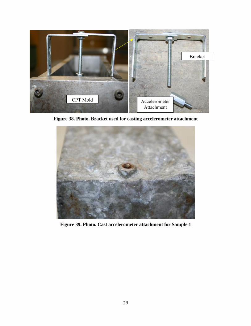
Alternative attachment techniques have been explored in an effort to improve robustness of the NIRAS technique. Casting a screw attachment into the sample was investigated to test whether improvements in consistency could be achieved. The very reactive Las Placitas aggregate was used in this assessment. The casting of the screw attachment was achieved using a bracket, which held the attachment during the casting, as shown in figure 38. Inconsistencies were noted in the embedment depth and bonding of the cast screw attachment to the concrete for the three samples, as shown in figure 39, figure 40, and figure 41. Consequently, the results were also varied. Figure 42 and figure 43 show the FFT and frequency shift for sample 1 at an early age, where the standard deviation (SD) is about 29 percent from the mean, but for a later age, shown in figure 44 and figure 45, the SD from the mean is only about 2 percent. Also, note that the accelerometer could not be attached using an adhesive in the same spot as the cast attachment, and this can also be a source of variability between the attachment methods.

Because the screw attachment was steel and could also be used as an attachment for a magnet, this coupling technique was also investigated. Figure 46 through figure 51 show the results at 65 days for all three samples with all three coupling techniques. The SD is 26.51 percent for figure 46 and figure 47, 19.92 percent for figure 48 and Figure 49, and 20.03 percent for figure 50 and figure 51.

Based on the current results, there does not seem to be an apparent advantage to casting a screw/magnet attachment into the specimens. In fact, looking at figure 50 and figure 51, some irregularities in the FFT signal are noticeable for the screw attachment that are not seen for the magnet or adhesive attachment. Consequently, for the remainder of the project, the focus will to increase the robustness of using an adhesive attachment; the adhesive attachment also has the advantage of being semi-permanent and can be readily applied to concrete cores.

29

Figure 38. Photo. Bracket used for casting accelerometer attachment

Figure 39. Photo. Cast accelerometer attachment for Sample 1

CPT Mold

Bracket

Accelerometer Attachment

30



31

Key — = Screw Linear Ft where η = 2.65

--- = Adhesive Linear Fit where η = 1.75

Figure 42. Graph. FFT and frequency shift in the frequency domain for Sample 1 at 23 days of age

Figure 43. Graph. FFT and frequency shift in linear format for Sample 1 at 23 days of age

32





33

Key — = Screw Linear Ft where η - 6.4684



Figure 47. FFT and frequency shift in linear format for Sample 1 at 65 days of age

34

Key — = Screw Linear Ft where η - 2.6125




35




Figure 51: Graph. FFT and frequency shift in linear format for Sample 3 at 65 days of age

Robustness of NIRAS Test Setup

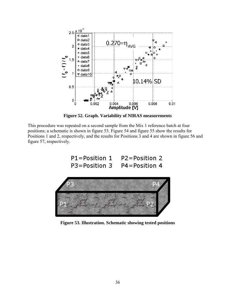
The consistency of the NIRAS setup was also tested by repeating measurements on the same sample 10 times on mature specimens in a brief time span, removing the accelerometer and re-gluing it each time the slope, which represents nonlinearity, was recorded. The sample tested was one of the Mix 1 reference samples (see table 2). The result is shown in figure 52, which demonstrates about 10-percent SD from the mean nonlinearity (AVG) .

36

Figure 52. Graph. Variability of NIRAS measurements

This procedure was repeated on a second sample from the Mix 1 reference batch at four positions; a schematic is shown in figure 53. Figure 54 and figure 55 show the results for Positions 1 and 2, respectively, and the results for Positions 3 and 4 are shown in figure 56 and figure 57, respectively.

Figure 53. Illustration. Schematic showing tested positions

AVG

37

Figure 54. Graph. Variability for Position 1


AVG

AVG

38



Note that the mean values for Positions 1 and 2 are very close together. This makes sense because these positions are on the same prism surface but at opposite ends, so the same vibration mode is being measured. The SD for these positions is also practically the same. However, this SD is higher than the previously reported 10 percent shown in figure 52. This may be because these positions had been previously tested very frequently and a debonder (e.g., acetone) was not always used to remove the old adhesive. This resulted in a deteriorated surface at those positions, which may explain the higher SD. Positions 3 and 4 were tested for the first time, so the surface condition was relatively smooth, and the results show a markedly improved SD. Also, as before, the mean value is very close for the two positions because they are on the same surface of the prism. The average nonlinearity for the 10 data sets for Positions 3 and 4 is higher than the nonlinearity for Positions 1 and 2. This result is expected because both the material itself and the

AVG

AVG

39

damage are not perfectly isotropic so these modes will not be purely symmetric. As a result, the excitation of a different surface can result in the vibration of a different cross-section property, which can cause measurement variability.

The samples used for these measurement variability experiments were undamaged samples with relatively low nonlinearity; therefore, a set of measurements was also made on a damaged sample with relatively high nonlinearity. The result, shown in figure 58, gives a linear relationship and an SD in measurements that are comparable to results for the sample with low nonlinearity. (Note that the y-axis scale for figure 58 is different than for figure 54 through figure 57.)

Figure 58. Graph. Variability for damaged sample (note difference in y-axis scale)

Validation of Linear Assumption

As noted in the theoretical background section of this report, the nonlinear parameter used in this study is extracted by assuming a linear relationship between frequency shift and strain amplitude. This is thought to hold true for low levels of strain amplitude. A question that arises from that assumption concerns the limit to which that statement holds true. This limit was tested on samples with relatively high (ASR-06) and low nonlinearity (Mix 4 reference, stored at ambient conditions). The results demonstrate that the limit is not the same for both samples. The highly nonlinear sample shown in figure 59 deviates from the linear relationship at a relatively low amplitude but there is no deviation for the sample with low nonlinearity, shown in figure 60. Note that both samples were excited to the same level of impact excitation but the response of a highly nonlinear specimen has lower amplitude than that of one with low nonlinearity owing to peak broadening (greater damping). These results demonstrate that for a highly nonlinear sample, the relationship between frequency shift and amplitude is linear for amplitudes lower than 5 x 10-3 volts The relationship remained linear for all levels of excitation for the sample with low nonlinearity. In all other measurements in this project, the impact excitation was kept low enough to avoid a nonlinear relationship between frequency shift and amplitude.

AVG

40

Figure 59. Graph. Results for higher amplitude excitation for ASR-06

Figure 60. Graph. Results for higher amplitude excitation for Mix 4 reference stored at ambient conditions

SETUP SUMMARY

These results show the ability of the nonlinear resonance techniques to distinguish the less damaged (i.e., lower slope) samples from the highly damaged (i.e., higher slope) samples and suggest the potential of this approach for damage assessment in concrete. Because the results of NIRAS are clear and consistent, the NIRAS technique has been applied to all the mixtures listed in table 3.

41

CHAPTER 5. PETROGRAPHIC METHODS

In addition to expansion measurements, a limited petrographic analysis is performed on companion CPT samples as a complementary assessment of the progression of damage. Companion samples for petrography were cast from each of the mixes tested by NIRAS and CPT. The petrographic examination relies on the use of a fluorescent stain that can be used to quickly identify the presence of ASR gel. The uranyl acetate staining technique was introduced by Natesaiyer and Hover, and it has also been appended to ASTM C856 Standard Practice for the Petrographic Examination of Hardened Concrete.(20,21) From previous studies, it has been determined that silica gel possesses the capability of adsorption of ions as well as ion exchange. When the ASR gel is formed in concrete, the cations present may include calcium, sodium, and potassium. Through ion exchange, the uranyl ion, in uranyl acetate stain solution, can replace the cations present in the gel. Because the uranyl ion fluoresces green when excited by ultraviolet radiation at 0.00001 inches (254 nm) (UV-C light), the silica gel in concrete can be easily identified with a UV-C light source after staining. However, it has been found that siliceous, not necessarily reactive, aggregates also fluoresce because the silica surface always contains free OH- groups with adsorbed cations, which can be replaced by the uranyl ion.(21) This can cause complications with the analysis of the images because the fluorescence of the aggregate can make it difficult to distinguish between the aggregate and reaction rims. Despite this limitation, the technique is still useful for tagging possibly relevant features in the microstructure, which simplifies the petrography.

PETROGRAPHIC SAMPLE PREPARATION

Whenever petrography is performed, a 0.5-inch-thick rectangular sample is cut, using a table saw, from the concrete prism. The sample is rinsed briefly with de-ionized water and placed in a fume hood, as a safety precaution to prevent inhalation. The 0.11 N uranyl acetate solution is applied to the freshly cut surface using a pipette and allowed to rest for 1 minute. Next, the surface is thoroughly rinsed with de-ionized water, and the sample is placed under a microscope. A heavy tarp is placed over the microscope instead of using a dark room. A UV lamp is used to illuminate the surface of the sample and a built-in camera (SPOT™ Insight color camera) is used to capture the image from the microscope (Leica® MZ6 stereomicroscope). The initial petrography was conducted using a handheld UV lamp (UVP Model UVSL-14P) and, in an effort to improve image quality, a higher-intensity pen-ray lamp (UVP Model 11SC-1), with short wavelength filter, has been used in the later stages of petrographic examination.

INTERPRETATION OF PETROGRAPHIC IMAGES

Note that the results presented in this report were obtained on unpolished sections. The loss of the gel was a concern at the start of the petrographic examination, and it was decided to forego polishing to limit this loss. However, in an effort to improve image quality, polishing was tried on an ASR damaged Las Placitas sample. Observation of fluorescing ASR gel suggests that the sample preparation methods used are appropriate for these types of samples. Figure 61 shows a representative unpolished stained section for a concrete prism with a reactive aggregate, and figure 62 shows a polished section for the same concrete prism (different section). The concrete prism is a recast version of Mix 2. Additional specimens for Mix 2 were cast to allow imaging during the initial stages of the reaction. When comparing the images in figure 61 and figure 62,

42

there does not appear to be any evidence of loss of ASR gel. In fact, figure 62 shows a relatively large crack that is still stained after polishing. When comparing the quality of the images, the unpolished section does not appear as clear as the polished section. For the unpolished section, it is difficult to achieve good focus, especially at higher magnifications, resulting in diminished image quality. For the polished section, the image is not only in focus but the stained features are more distinct. In the polished section, it is possible to see microcracks at the edge of the macrocrack. Based on these results, for future petrographic examination, the samples will be polished before staining.

500 microns = 0.19685 inches

Figure 61. Photo. Unpolished stained section

500 microns = 0.19685 inches

Figure 62. Photo. Polished stained section

43

CHAPTER 6. RESULTS

EXPANSION RESULTS

This section presents the expansion measurement results for the concrete mixtures described in table 2. Note that in this study, the expansion measurements are taken more frequently than required in the ASTM C1293 standard. Figure 63 shows the results of the expansion measurements for the HR mixtures. Comparing the results from ASTM C1260 (table 2) and the measured expansions in figure 63, it is evident that there is good agreement for the classification of the HR mixtures (i.e., mixes 2 through 5). Figure 64 shows results up to 100 days to facilitate identification of the specimen age at which the 0.04-percent expansion limit, indicating aggregate reactivity, is crossed. Mixes 2 through 5 have expansions that cross this limit during the test period. Also, the relatively rapid expansion rate for these mixes further suggests the relatively high reactivity of these aggregates. There also appears to be some observation of more rapid and, in one case, larger expansion when the reactive aggregate is crushed and used as the fine in the mixture. This is demonstrated when comparing mixes 2 and 3 as well as mixes 4 and 5. However, an exception to this observation is the behavior for Mix 4 when recast, to better evaluate the early (<100 days of age) expansion behavior; that sample set has an uncharacteristically high rate of expansion compared with previous results for Mix 4. The underlying cause for this difference in behavior between the two sample sets is not clear; it may simply be related to the variability inherent in concrete and in reactive aggregates in particular.

Results for the NR Mix 1, the MR mixes 6 and 7, and SCM-containing mixes 8 and 9 are presented in figure 65. The average expansion of mixes 1 and 6 has not crossed the expansion limit at 1 year; therefore, these are classified as nonreactive by the CPT standard. Mix 6 was expected to experience more expansion than Mix 1 because, according to ASTM C1260, the aggregate in Mix 6 was classified as innocuous or potentially deleterious. According to these concrete prism results, the aggregate is nonreactive but it does come very close to the expansion limit, demonstrating perhaps some of the challenges associated with determining reactivity through expansion measurements alone. The 25-percent replacement of cement with fly ash (FA) in mixes 8 and 9 appears to be effective in mitigating expansion with the Spratt aggregate because the expansion limit has not been crossed. For comparison, mixes 4 and 5, using the same aggregate, crossed the limit before 100 days. Mix 7 crossed the limit at about 150 days and can be classified as reactive using the CPT standard.

44

0

0.1

0.2

0.3

0.4

0.5

0.6

0.7

0 50 100 150 200 250 300 350 400

Expan

sion (%)

Specimen Age (days)

Mix 2 HR (Las Placitas)/ NR Mix 3 NR/ HR (Las Placitas)

Mix 4 HR (Spratt)/ NR Mix 4 (recast)

Mix 5 NR/ HR (Spratt) Reactive Agg Expansion Limit

Figure 63. Graph. ASTM C1293 expansion results up to 400 days

0

0.05

0.1

0.15

0.2

0.25

0 20 40 60 80 100

Expan

sion [%

]

Specimen Age [days]

Mix 2 HR (Las Placitas)/ NR

Mix 3 NR/ HR (Las Placitas)

Mix 4 HR (Spratt)/ NR

Mix 4 (recast)

Mix 5 NR/ HR (Spratt)

Reactive Agg Expansion Limit

Figure 64. Graph. ASTM C1293 expansion results up to 100 days

45

Figure 65. Graph. ASTM C1293 expansion results up to 750 days for NR, MR, and SCM mixes

NIRAS RESULTS

NIRAS results are presented in a similar manner as the expansion measurements, that is the average measured nonlinearity, performed on the same three samples as CPT expansion, is plotted versus age at each test date. With this representation, the nonlinearity parameter is shown as a function of time that samples were exposed to ASTM C1293 testing conditions. For Mix 4, note that because the NIRAS measurements did not start on Mix 4 until after the expansion was greater than 0.04 percent, that mix was recast to gather early age data for that mix.

As an example of how the nonlinearity of a given sample at a given age is determined, consider Mix 3 at 47 days. The data analysis process for one of the Mix 3 prisms is shown in figure 66. The impact response for 10 separate hits is recorded and converted to the frequency domain, as described previously. The frequency shift is then normalized and plotted against the excitation, as shown in figure 66. The nonlinearity parameter ( ) is the slope of the data on this plot; in this case, is found to be 5.6082. For the other samples, the nonlinearity parameters were measured to be 7.2799 and 5.6941. The average of these nonlinearity parameters is 6.19.

46

Figure 66. Graph. Example of extraction of nonlinearity parameter for Mix 3 at 47 days

This average nonlinear parameter, along with SD at each measurement age, is then plotted versus age, as in figure 67. The average nonlinearity parameter of 6.19 at 47 days can be seen in figure 67 and corresponds to the maximum nonlinearity measured for Mix 3. Figure 67 shows the results up to 750 days while figure 68 shows a more detailed view, only up to 100 days, to better show early age behavior.

From these results, performed on a limited range of aggregates and with a limited range of binder compositions, a preliminary limit of 0.2 during the standard test duration has been proposed to distinguish between alkali reactive and non-reactive aggregates, cast, and tested according to ASTM C1293. Figure 67 shows this limit. However, significant further investigation—including ruggedness testing, round-robin testing of precision and bias, and a comprehensive assessment of more aggregate types—is clearly needed to determine the microstructural changes that contribute nonlinearity, as well as to better assess what level of nonlinearity can be used to distinguish between innocuous aggregates and those detrimental to long-term performance.

The results show that the NIRAS technique confirms the ASTM C1293 reactivity classification based on expansion results for the HR mixtures. For aggregates initially classified as HR, as with AMBT, measures of CPT expansion and nonlinearity are in agreement, as summarized in table 5. However, in some cases, there is an indication of earlier detection of reactivity using NIRAS. Comparing Mix 2 in figure 64 and figure 68, it can be seen that the NIRAS technique is capable of identifying ASR sooner than the expansion measurements; nonlinearity is detected at 8 days while the expansion limit is crossed at about 25 days. However, further investigations are clearly needed in this area to determine what kind of microstructural changes cause nonlinearity as well as what level of nonlinearity can be considered detrimental. These investigations will enable us to describe the damage in concrete in a more quantitative manner and to give a definitive criterion for reactivity of an aggregate, considering its microstructure and chemical properties.

47

Figure 67. Graph. NIRAS results up to 750 days

Figure 68. Graph. NIRAS results up to 100 days

48

Table 5. Summary of reactivity classifications based on AMBT, CPT, and NIRAS

Sample

Aggregate reactivity based on

ASTM C1260

Aggregate reactivity based on

ASTM C1293

Aggregate reactivity based on NIRAS

Mix 1 Innocuous Nonreactive Nonreactive

Mix 2 Potentially Deleterious

Reactive Reactive


Reactive Reactive


Reactive Reactive


Reactive Reactive

Mix 6 Innocuous or Potentially Reactive

Nonreactive Nonreactive


Reactive Nonreactive

Table 5 also summarizes results for the NR Mix 1 and the MR Mix 6. For both Mix 1 and Mix 6, the average expansion of the specimens at 1 year is very close to the 0.04-percent expansion limit in ASTM C1293 but does not exceed that limit, indicating a nonreactive aggregate by that measure. The classification of aggregate in Mix 6 is more ambiguous because it exceeded the lower 0.1-percent expansion limit in AMBT. NIRAS shows the nonlinearity of both Mix 1 and Mix 6 specimens has remained very close to zero throughout the year of testing, indicating these are nonreactive aggregate. While the expansion for any concrete sample, including the nonreactive mixes, increases as the duration of the test increases, the nonlinearity does not change for a nonreactive aggregate, providing a more definitive and accurate result.

The only mix for which the nonlinearity measurements are contrary to expansion results is Mix 7, as shown in table 5. The expansion limit has been crossed for that mix but nonlinearity remains negligible throughout the test period. Petrography has been performed on this mix in an attempt to assess the validity of the various results for this aggregate. Those results are presented in the “Petrography Results” section of this chapter.

Nonlinearity was also measured on reference samples held at ambient laboratory conditions (i.e., not exposed to ASTM C1293 accelerated environmental conditions). Figure 69 shows those results. All the values of nonlinearity for reference mixtures are considerably lower than what measurements for reactive mixtures that have undergone CPT. For example, the results for Mix 4, for both CPT and reference samples, are shown in figure 70 and figure 71. Notice that in addition to a negligible frequency shift, the reference sample has a sharper resonance at a higher frequency due to lower attenuation.

49

Figure 69. Graph. NIRAS results for reference mixes

Figure 70. Graph. Nonlinearity comparison between reference and tested samples for HR Mix 4 at 250 days

50

Figure 71. Graph. Comparison between reference and tested samples for HR Mix 4 at 250 days in the frequency domain

It is interesting to note that in figure 68 and figure 69, mixtures tested at the first day show some nonlinearity that then decreases down to zero through subsequent testing. This can be caused by the continued hydration of the cement after demolding, which decreases the inherent material nonlinearity by eliminating defects present initially (i.e., before the material nonlinearity due to ASR becomes dominant). The results for the reference mixes are surprising for the NR mixture, because slightly lower nonlinearity is detected for the specimens subjected to CPT. (However, it should be noted that in both environments, the nonlinearity for the NR mix is very low.) The difference in the measurements could be related to variations in inherent defects between the two sample groups or, perhaps more likely, by more limited cement hydration during storage at drier ambient conditions, compared with the moist conditions during CPT. Because the CPT sample group has abundant moisture available to promote cement hydration (which could fill early age cracking and porosity), NR concrete can achieve more complete hydration and hence lower nonlinearity than the reference sample group, for which the drier conditions would limit hydration. Because the reference samples undergo only 1 day of moist curing, it is possible that the inadequate hydration can be the cause of the slight nonlinearity in the nonreactive reference mixtures. Overall, however, the results indicate that it may be possible to extend the use of this technique to investigations of the cement hydration process, as well as self-healing in cementitious systems.

In addition, the observed decrease in the nonlinearity parameter for reactive mixes at later ages should be considered. This underlying cause for the decrease at later ages is not yet fully understood, but it is postulated this may be related to cracks growing to larger sizes (i.e., wider cracks). The measured nonlinearity comes from the nonlinear behavior of cracks, through the interaction of crack surfaces. When a crack becomes too large, the crack faces may no longer interact and, as a result, no longer contribute to nonlinearity. It is important to notice that this decrease in nonlinearity appears to occur at about the same time the expansion rate starts to decrease and level off. Perhaps the same phenomenon is responsible for the eventual decrease in expansion rate and decrease in nonlinearity observed in the results.

51

Another way to represent the nonlinearity data—and one that shows even greater distinction between the reactive and nonreactive aggregates—is through a measure of accumulated damage, c . This approach is described in chapter 2. Figure 72 shows accumulated damage for all samples, while figure 73 shows a detailed view of the results for the NR and MR mixtures. Using the accumulated damage for these NR and MR mixtures, some distinction can be made between the mixtures that was not clear from the instantaneous nonlinearity in figure 67 and figure 68. One observation from comparing these results is that nearly the same levels of accumulated damage and instantaneous nonlinearity have developed in HR Mix 4 (initial and recast samples). This result can be seen in figure 67, figure 68, and figure 72. The expansion measurements, figure 63 and figure 64, show more variable results when comparing the recast Mix 4 with the initially cast batch. However, with both methods of assessment, the aggregate is clearly reactive.

As noted earlier, the expansion measurements seem to indicate a faster rate of reaction when the reactive aggregate is used as a fine aggregate as compared with its use as a coarse aggregate; an exception is the case of the recast Mix 4. With the NIRAS measurements, particularly in the assessment of accumulated damage, there is no observable trend with the size of the reactive aggregate. This can be beneficial in laboratory testing because there is no effect of gradation on the results of reactivity classifications, offering benefits for the assessment of job mixtures and potentially eliminating the needed for crushing and/or grading prior to assessment.

The SD, represented by error bars in figure 67 and figure 68, shows the variability among the measurements made on three samples for each mix at each age. Both the expansion measurements and measurements of c have a general trend of increasing SD with increasing expansion or nonlinearity. Because of inherent heterogeneities, the cast prisms are not identical to each other, even within the same mix. As a result, each sample represents a different material system that can accumulate damage in different ways. Because of the high sensitivity of NIRAS, the SD is larger for reactive mixes.

Because the lowest amplitude impact is assumed to be the approximate linear resonance frequency, this measure can also be used to track changes to the specimens. In general, these data, shown in figure 74, complement the nonlinearity measurements. Examining data for mixes 5, 8, and 9 from figure 67, figure 68, and figure 74, it is observed that these mixes start with a low linear resonance frequency and relatively high nonlinearity after demolding. Subsequently, the linear resonance frequency increases (presumably because of an increase in elastic modulus due to hydration) and nonlinearity decreases. This data supports the postulated explanation for relatively high initial nonlinearity and slightly higher nonlinearity for nonreactive reference mixes. Overall, an observed decrease in linear resonance frequency also relates to an increase in nonlinearity, demonstrating an inverse relationship between changes in linear resonance frequency and nonlinearity parameter. It is important to observe that the changes in nonlinearity are significantly larger than the changes in the linear resonance frequency. This comparison, demonstrates that nonlinearity can be used to more accurately assess changes in the specimens than changes in linear resonance frequency.

52

Figure 72. Graph. Cumulative nonlinearity

Figure 73. Graph. Cumulative nonlinearity for NR and MR mixes

53

Figure 74. Graph. Changes in linear resonance frequency

CORED SAMPLE RESULTS

To assess whether the NIRAS technique might be used to examine ASR damage in the field or on samples obtained from in-service structures, cored samples obtained from two different pavements were also tested. The cores were supplied by the Georgia Department of transportation (GDOT). One core was taken from I-75 and another was taken from Highway (HWY) 316. The concrete from HWY 316 is suspected to have ASR damage, while that from I-75 was not expected to have ASR, based on external petrographic analysis. The cores were tested in the same manner and with the same setup as described in Chapter 4. The nonlinearity results for I-75 and HWY 316 are shown in figure 75 and figure 76, respectively.

These results clearly show that HWY 316 has a significantly higher nonlinear parameter, indicating that it has experienced damage. While the cause of damage is unclear, the measurements suggest that the result is an extensively microcracked road. This technique offers an extremely rapid and non-subjective evaluation of cores that can be used to evaluate field concrete.

54

Figure 75. Graph. Nonlinear measurement results on I-75 core

Figure 76. Graph. Nonlinear measurement results on HWY 316 core

PETROGRAPHY TO COMPLEMENT NIRAS RESULTS

As described in chapter 5 of this report, complementary assessment of the progression of damage in the concretes was performed through petrographic assessment of concrete prisms from various

55

mixes and after various CPT durations. These results can be used to better understand the data obtained through CPT and NIRAS evaluation.

For HR Mix 2, the results of the preliminary petrographic examination, using the uranyl acetate stain on a prism, are shown in figure 77 and figure 78. For this mix, a set of five prisms was recast—with three used for expansion and two for petrography—to obtain early age images. Comparing figure 77 and figure 78 shows a clear difference in the petrographic features at different specimen ages. At 1 day, the representative cross-section in figure 77 shows only a light staining of the paste but no signs of ASR gel. At 9 days, as shown in figure 78, there is clear evidence of reaction rims forming around some aggregates, indicating ASR activity. These results are consistent with the nonlinearity results for Mix 2, for which the measurements show a detectable nonlinearity at the first measurement at 8 days. Figure 79 shows the expansion measurements for the originally cast Mix 2 samples and for the recast Mix 2 set. In addition, the nonlinearity of the original Mix 2 samples is plotted on the secondary axis. These results show that nonlinearity measurements appear to indicate reactivity at earlier ages than the expansion results; that is, the expansion limit is not crossed until about 13 days and 20 days for the recast and original Mix 2 samples, respectively, while the proposed nonlinearity limit or 0.2 was already exceeded by the time of the first NIRAS measurement, at 8 days.

At later ages, petrographic examination shows substantial staining throughout the concrete matrix, making it difficult to determine which microstructural changes are most influencing the nonlinearity measurements. As mentioned earlier, Mix 4 had been recast to gather nonlinearity data for the early ages because this mixture had been originally cast before the development of a nonlinear measurement setup. In addition to gathering nonlinear data, expansion measurements were also collected for these recast samples, and petrography was performed regularly. The expansion and nonlinearity results are shown together in figure 80.

1 mm = 0.03937 inches

Figure 77. Photo. Petrographic image for Mix 2 at 1 day

56

1 mm = 0.03937 inches

Figure 78. Photo. Petrographic image for Mix 2 at 9 days

Figure 79. Graph. Comparison of expansion and nonlinearity results for Mix 2

57

Figure 80. Graph. Comparison of expansion and nonlinearity results for Mix 4

The results show that the recast Mix 4 prisms had a considerably higher expansion rate, crossing the limit at only 20 days while the originally cast mixture crossed at about 95 days. For the NIRAS measurements, the nonlinearity starts to develop at about 50 days. At 12 days, although there is a small amount of staining of the paste, there is no fluorescence, as shown in figure 81 and figure 82. At 26 days, overall, there is little fluorescence, with only a few instances of fluorescence shown in figure 83 and figure 84. At 40 days, there is still little fluorescence in the sample; only a few instances are found, shown in figure 85 and figure 86. These results are not consistent with expansion results because much more fluorescence is expected once the expansion limit is crossed. Note the nonlinearity remains low for these ages. At 54 days, there is significantly more fluorescence but it appears inside the aggregates, which was not observed in other aggregate sources examined (see figure 87 and figure 88). At about this time, nonlinearity starts to increase. At 62 days, the fluorescence is even more common and consistent with the increase in nonlinearity (see figure 89 and figure 90).

58

1 mm = 0.03937 inches

Figure 81. Photo. Image 1 of recast Mix 4 at 12 days

1 mm = 0.03937 inches


1 mm = 0.03937 inches


59

1 mm = 0.03937 inches


1 mm = 0.03937 inches

Figure 85. Photo. Image 1 recast Mix 4 at 40 days

1 mm = 0.03937 inches

Figure 86. Photo. Image 2 recast Mix 4 at 40 days

60

1 mm = 0.03937 inches


1 mm = 0.03937 inches


1 mm = 0.03937 inches


61

1 mm = 0.03937 inches


Petrography was also performed on Mix 7. Again, all samples were recast. At 218 days, after the expansion limit had been crossed, as shown in figure 91 and figure 92, some staining of certain aggregates is apparent but there is no evidence of reaction rims or cracks. This technique was also applied to the reference Mix 7 for comparison, as shown in figure 93 and figure 94. When compared, the photos of Mix 7 and those of reference Mix 7 show little difference between the features of the concrete exposed to accelerated conditions and that stored at ambient conditions. This petrographic examination does not provide evidence of ASR and, as a result, confirms the nonlinearity results but contradicts expansion results.

1 mm = 0.03937 inches


62

1 mm = 0.03937 inches


1 mm = 0.03937 inches

Figure 93. Photo. Image 1 for recast reference Mix 7 at 218 days

1 mm = 0.03937 inches

Figure 94. Photo. Image 2 for recast reference Mix 7 at 218 days

63

CHAPTER 7. CONCLUSIONS AND RECOMMENDATIONS

CONCLUSIONS

1. NIRAS measurements have shown a clear distinction between reactive and nonreactive aggregates and among concrete mixtures containing reactive aggregate with and without mitigation for ASR. For HR cases, there is evidence of earlier detection of ASR-related damage with the NIRAS testing technique than with concrete prism expansion.

2. The NIRAS measurement setup has proven to be a robust and accurate measurement technique. The variability between successive measurements has been shown to be less than 20 percent overall and less than 10 percent with a prepared adhesion surface.

3. NIRAS has also been proven to be a powerful nondestructive testing (NDT) tool to rapidly detect microcrack-type damage (regardless of the cause) in concrete in an early stage of the material degradation. Based on the current body of research, this test should be used as a supplement to other standard testing. Additional research and testing can be used to assess whether NIRAS can be used as an alternative test.

4. With some aggregate types, a higher rate of expansion is measured with aggregate that has been crushed than in the as-received condition, showing a potential effect of aggregate size. The NIRAS measurements, however, do not appear to be affected by the reactive aggregate size and show the potential to be used to evaluate job-specific aggregates, while also eliminating the need for the time-consuming crushing and grading processes.

5. Complementary petrography, performed by staining the concrete samples with uranyl acetate, was used to confirm the presence of ASR gel and cracking within the samples. Based on this lack of fluorescence, gel, and cracking, one aggregate identified as non-reactive through NIRAS was confirmed to be non-reactive, despite having been identified as potentially deleterious and reactive through expansion testing. Further petrographic analysis to complement expansion and NIRAS testing will contribute to improving the understanding of ASR as well as to improving the understanding of the correlation between the results of NIRAS and expansion testing.

6. Two nonlinearity parameters are defined: one () that characterizes the rate of damage development at a certain age and another (c) that characterizes the amount of damage accumulated up until that time. Based on the experimental results for a limited number of aggregates—albeit with various levels of reactivity—it is proposed that the aggregate under assessment can be considered alkali reactive if the nonlinearity parameter of its concrete prism specimen measures 0.2 or more at any time during the 12-month test period. Nonlinearity parameters between 0.05 and 0.2 may suggest some potential for ASR, and the aggregate should be further evaluated. These proposed limits, however, must be verified through a more comprehensive evaluation of a broader range of aggregates and also through round-robin testing.

64

RECOMMENDATIONS FOR FURTHER RESEARCH

This research has shown that the NIRAS technique has potential as a powerful method for non-destructive evaluation of concrete in the laboratory, in cored samples, and potentially in the field. Although applications for detection of ASR-induced damage are the focus of this research, results here suggest the technique could be further developed for detection and quantification of cumulative damage due to various causes (e.g., fatigue, freeze/thaw, sulfate attack, reinforcement corrosion) and also for examination of hydration and self-healing in concrete.

With regard to ASR, further efforts are needed in several areas. First, additional research is needed for continued development and validation of the NIRAS technique with a broader range of aggregate mineralogies and reactivities, including assessment of more aggregates when assessment by AMBT and CPT is ambiguous. In this research, the nonlinearity measurements for an aggregate that was near the expansion limit and was determined to be potentially deleterious and reactive by AMBT and CPT, respectively, showed negligible nonlinearity. The lack of ASR damage was confirmed through petrographic assessment. Assessment of more aggregates that are known to be challenging to classify is warranted, in particular.

In addition, with further NIRAS assessment it is also important to continue to assess the relationship between microstructural changes and changes in nonlinearity, as well as to compare results with standard expansion tests and field performance. This correlation among the various measures aids not only in the classification of the aggregates, but also in the continued assessment of the proposed limit on nonlinearity. In addition, a limit on cumulative nonlinearity might also result from further research and development efforts. In particular, the age at which aggregate reactivity is identified by NIRAS and expansion testing should be compared over a broader range of aggregates to provide additional understanding of the potential benefits of NIRAS for early and reliable detection of reactive aggregates.

Based on those results, a critical next step would be to build a predictive model that captures the physics of the damage evolution of ASR. This physics- and chemistry-based material model could be used to interpret these experimental results and thus predict the resonance response of an ASR-damaged specimen or concrete. This work would result in refinements in the accuracy of the identification of reactive aggregate and form the foundation for a device for detection of ASR in the field.

A round-robin test series should also be initiated for concrete prism samples. Such a series would involve several laboratories using the NIRAS technique to measure nonlinearity and CPT expansion in a pre-determined set of aggregates; these might include some of those identified through continued research on aggregates whose reactivity is “ambiguous.” Results could be used to establish precision and bias for the test and to refine a standard test procedure.

Because the NIRAS method appears to be insensitive to reactive aggregate size and because the technique was successfully applied to both ordinary concrete and concrete with SCMs, the method appears to have potential as a technique for screening job mixes. A research program should be established to measure change in nonlinearity over a broad range of concrete, varying the aggregate reactivity and gradation, water-to-cement ratio, and binder composition. Exposure could be done using CPT or other accelerated testing appropriate for concrete.

65

REFERENCES

1. Farny, J.A. and Kosmatka, S.H., “Diagnosis and Control of Alkali-Aggregate Reactions in Concrete,” Portland Cement Association IS413, 1997.

2. Mehta, P.K. and Montiero, P.J.M., Concrete: Microstructure, Properties, and Materials, 3rd ed. New York: McGraw-Hill. 2006.

3. ASTM C1293, “Standard Test Method for Determination of Length Change of Concrete Due to Alkali-Silica Reaction,” ed. West Conshohocken, PA: ASTM International. 2008.

4. ASTM C1260, “Standard Test Method for Potential Alkali Reactivity of Aggregates (Mortar-Bar Method),” ed. West Conshohocken, PA: ASTM International. 2007.

5. Folliard, K., Thomas, M.D.A., and Kurtis, K.E., “Guidelines for the Use of Lithium to Mitigate or Prevent ASR in Concrete,” Publication No. FHWA-RD-03-047, Federal Highway Administration. 2003.

6. Haha, M. B., Gallucci, E., Guidoum, A., and Scrivener, K.L., “Relation of Expansion Due to Alkali Silica Reaction to the Degree of Reaction Measured by SEM Image Analysis,” Cement and Concrete Research, Vol. 37, pp. 1,206–1,214. 2007.

7. Nagy, P.B., “Fatigue Damage Assessment by Nonlinear Ultrasonic Materials Characterization,” Ultrasonics, Vol. 36, pp. 375–381. 1998.

8. Van Den Abeele, K.E.A., Johnson, P.A., and Sutin, A., “Nonlinear Elastic Wave Spectroscopy (NEWS) Techniques to Discern Material Damage, Part I: Nonlinear Wave Modulation Spectroscopy (NWMS),” Research in Nondestructive Evaluation, Vol. 12, pp. 17–30. 2000.

9. Chen, J., Jayapalan, A.R., Kim,J.-Y., Kurtis, K.E., and Jacobs, L.J., “Rapid Evaluation of Alkali-Silica Reactivity of Aggregates Using a Nonlinear Resonance Spectroscopy Technique,” Cement and Concrete Research, Vol. 40, pp. 914–923. 2010.

10. Payan, C., Garnier,V., Moysan, J., and Johnson, P.A., “Applying Nonlinear Resonant Ultrasound Spectroscopy to Improving Thermal Damage Assessment in Concrete,” Journal of the Acoustical Society of America, Vol. 121, pp. EL125–EL130. 2007.

11. Van Den Abeele, K. and De Visscher, J., “Damage Assessment in Reinforced Concrete Using Spectral and Temporal Nonlinear Vibration Techniques,” Cement and Concrete Research, Vol. 30, pp. 1,453–1,464. 2000.

12. Muller, M. Sutin, A., Guyer, R., Talmant, M., Laugier, P., and Johnson, P.A., “Nonlinear Resonant Ultrasound Spectroscopy (NRUS) Applied to Damage Assessment in Bone,” Journal of the Acoustical Society of America, Vol. 118, pp. 3,946–3,952. 2005.

13. Van Den Abeele, K.E.A., Carmeliet, J., Ten Cate, J.A., and Johnson, P.A., “Nonlinear Elastic Wave Spectroscopy (NEWS) Techniques to Discern Material Damage, Part II: Single-Mode

66

Nonlinear Resonance Acoustic Spectroscopy,” Research in Nondestructive Evaluation, Vol. 12, pp. 31–42. 2000.

14. Chen, J., Jayapalan, A.R., Kim, J.-Y., Kurtis, K. E., and Jacobs, L.J., “Nonlinear Wave Modulation Spectroscopy Method for Ultra-Accelerated Alkali-Silica Reaction Assessment,” ACI Materials Journal, Vol. 106, pp. 340–348. 2009.

15. Chen, X.J., Kim, J.-Y., Kurtis, K.E., Qu, J., Shen, C.W., and Jacobs, L.J., “Characterization of Progressive Microcracking in Portland Cement Mortar Using Nonlinear Ultrasonics,” NDT and E International, Vol. 41, pp. 112–118. 2008.

16. Morris, W.L., Buck, O., and Inman, R.V., “Acoustic Harmonic Generation Due to Fatigue Damage in High-Strength Aluminum,” Journal of Applied Physics, Vol. 50, pp. 6,737–6,741. 1979.

17. Solodov, I.Y. and Korshak, B.A., “Instability, Chaos, and “Memory” in Acoustic-Wave-Crack Interaction,” Physical Review Letters, Vol. 88, pp. 143,031–143,033. 2002.

18. ASTM C215, “Standard Test Method for Fundamental Transverse, Longitudinal, and Torsional Resonant Frequencies of Concrete Specimens,” ed. West Conshohocken, PA: ASTM International. 2008.

19. ASTM E1876, “Standard Test Method for Dynamic Young’s Modulus, Shear Modulus, and Poisson’s Ratio by Impulse Excitation of Vibration,” ed. West Conshohocken, PA: ASTM International. 2009.

20. ASTM C856, “Standard Practice for Petrographic Examination of Hardened Concrete,” ed. West Conshohocken, PA: ASTM International. 2004.

21. Natesaiyer, K. and Hover K.C., “Insitu Identification of ASR Products in Concrete,” Cement and Concrete Research, Vol. 18, pp. 455–463. 1988.

HRDI-60/10-13(600)ERecycledRecyclable

Documents

Accelerated Determination of ASR Susceptibility During … · Krzysztof J. Lesnicki, Jin-Yeon Kim, Kimberly E. Kurtis, and Laurence J. Jacobs 8. Performing Organization Report No