A weak trapezoidal method for a class of stochastic differential

COMMUN. MATH. SCI. c© 2011 International Press

Vol. 9, No. 1, pp. 301–318

A WEAK TRAPEZOIDAL METHOD FOR A CLASS OF

STOCHASTIC DIFFERENTIAL EQUATIONS∗

DAVID F. ANDERSON† AND JONATHAN C. MATTINGLY‡

Abstract. We present a numerical method for the approximation of solutions for the classof stochastic differential equations driven by Brownian motions which induce stochastic variationin fixed directions. This class of equations arises naturally in the study of population processesand chemical reaction kinetics. We show that the method constructs paths that are second orderaccurate in the weak sense. The method is simpler than many second order methods in that itneither requires the construction of iterated Ito integrals nor the evaluation of any derivatives. Themethod consists of two steps. In the first an explicit Euler step is used to take a fractional step. Theresulting fractional point is then combined with the initial point to obtain a higher order, trapezoidallike, approximation. The higher order of accuracy stems from the fact that both the drift and thequadratic variation of the underlying SDE are approximated to second order.

Key words. Weak trapezoidal, error analysis, reaction networks, higher-order methods, stochas-tic differential equations, numerical methods.

AMS subject classifications. 60H35, 65C30, 65L20.

1. Introduction

We consider the problem of constructing accurate approximations on boundedtime intervals to solutions of the following family of stochastic differential equations(SDEs)

dX(t) = b(X(t))dt+

M∑

k=1

σk(X(t)) νk dWk(t),

X(0) = x ∈ Rd, (1.1)

where b : Rd → Rd, σk : R

d → R≥0, νk ∈ Rd, and Wk(t) are one-dimensional Wiener

processes. Thus, randomness enters the system in fixed directions νk, but at variablerates σk(X(t)). Precise regularity conditions on the coefficients will be presented withour main results in Section 2.

The algorithm developed in this paper is a trapezoidal-type method and consistsof two steps; in the first an explicit Euler step is used to take a fractional step and inthe second the resulting fractional point is used in combination with the initial point toobtain a higher order, trapezoidal like, approximation. We will prove that the methoddeveloped is second order accurate in the weak sense. Because the method developedhere produces single paths, it is natural to allow variable step-sizes; this is in contrastto Richardson extrapolation techniques ([20]). Finally, it is important to note thatwhile the method presented in this paper is applicable to only a sub-class of SDEs,that sub-class does include systems whose diffusion terms do not commute, which isa classical simplifying assumption to obtain higher order methods (see [9, 14]).

∗Received: June 17, 2009; accepted (in revised version): June 10, 2010. Communicated by WeinanE.

†Department of Mathematics, University of Wisconsin-Madison, Madison, Wi. 53706, USA ([email protected]).

‡Department of Mathematics, Center of Nonlinear and Complex systems, Center for Theoreticaland Mathematical Science, and Department of Statistical Science, Duke University, Durham, N.C.27708, USA ([email protected]).

301

302 A WEAK TRAPEZOIDAL METHOD FOR STOCHASTIC DIFFERENTIAL EQUATIONS

The method we propose is in some sense similar to the classical predictor- correc-tor. There have already been a number of such methods proposed in the stochasticcontext to produce higher-order methods (see [18, 19, 5]). In a general way, all ofthese methods require the simulation of iterated Ito integrals and sometimes needderivatives of the diffusion terms. If one only cares about weak accuracy, it is possibleto use random variables which make these calculations easier and computationallycheaper. That being said, the complexity and cost of such calculations is one of themain impediments to their wider use. By assuming a certain structure for (1.1), weare able to develop a numerical method which we hope is more easily applied andimplemented.

Though a specific structure of (1.1) is assumed, it is a structure which arises nat-urally in a number of settings. For example, our method will be applicable wheneverd = 1. Also, we note that diffusion approximations to continuous time Markov chainmodels of population processes, including (bio)chemical processes, satisfy (1.1). Asstochastic models of biochemical reaction systems, and, in particular, gene regulatorysystems, are becoming more prevalent in the science literature, developing algorithmsthat utilize the specific structure of such models has increased importance [1, 2].Furthermore, in Section 8 we quote a result from the literature which states thatany system with uniformly elliptic diffusion can be put in the form of (1.1) withoutchanging its distribution.

The topic of this paper is a method that produces a weak approximation ratherthan a strong approximation in that the approximate trajectory is produced withoutreference to an underlying Wiener process trajectory. We see this as an advantage.Except for applications such as filtering or certain problems of collective motion forstochastic flows, one is usually simply interested in generating an accurate draw fromthe distribution on C([0, T ],Rd) induced by (1.1). This is different than accuratelyreproducing the Ito map W 7→ X(t,W ) implied by (1.1). The latter is referred to asstrong approximation. In our opinion such approximations are usually unnecessaryand lead to a concept of accuracy which is unnecessarily restrictive. In [7], it isdiscussed that without accurately estimating second order Ito integrals one cannotproduce a strong method of order greater then 1/2. If the vector fields commute, thenthis restriction does not apply and higher order strong methods are possible. Whilethe term “strong approximation” is quite specific, the term “weak approximation”is used for a number of concepts. Here we mean that the joint distribution of thenumerical method at a fixed number of time points converges to the true marginaldistribution as the numerical grid converges to zero. If this error goes to zero at a rateequal to the numerical mesh size raised to the power p in some norm on measures,then we say the method is of order p. This should be contrasted with talking aboutthe rate at which a given function of the path converges.

The outline of the paper is as follows. In Section 2 we present our algorithmtogether with our main results concerning its weak error properties. In Section 3we give the intuition as to why the method should work. In Section 4 we give thedelayed proof of the local error estimates for the method which were stated in Sec-tion 2. In Section 5 we provide examples illustrating the performance of the proposedalgorithm. In Section 6 we discuss the effect of varying the size of the first fractionalstep of the algorithm. In Section 7 we compare one step of the algorithm to one stepin a Richardson extrapolation type algorithm. In Section 8 we show how, at leasttheoretically, the method can be applied to any uniformly elliptic SDE. Finally, anappendix contains a tedious calculation needed in Section 4.

D.F. ANDERSON AND J.C. MATTINGLY 303

2. The numerical method and main results

Throughout the paper, we let X(t) denote the solution to (1.1) and Yi denotethe computed approximation at the time ti for the time discretization 0 = t0 < t1 <· · · . We begin both from the same initial condition, namely X(0) = Y0 = x0. Let

η(i)1k , η

(i)2k : k ∈ 1, . . . ,M, i ∈ N

be a collection of mutually independent Gaussianrandom variables with mean zero and variance one. It is notationally convenient todefine [x]+ = x ∨ 0 = maxx, 0.

We propose the following algorithm to approximate the solutions of (1.1).

Algorithm. (Weak θ-Midpoint Trapezoidal ) Fixing θ ∈ (0, 1), we define

α1def

=1

2

1

θ(1− θ)and α2

def

=1

2

(1− θ)2 + θ2

θ(1− θ). (2.1)

Next, fixing a discretization step h, for each i ∈ 1, 2, 3, . . . we repeat the following

steps in which we first compute a θ-midpoint y∗ and then the new value Yi:

Step 1. y∗ = Yi−1 + b(Yi−1)θh+M∑

k=1

σk(Yi−1) νk η(i)1k

√θh

Step 2.

Yi = y∗ + (α1b(y∗)− α2b(Yi−1))(1− θ)h

+M∑

k=1

√

[

α1σ2k(y

∗)− α2σ2k(Yi−1)

]+νk η

(i)2k

√

(1− θ)h.

Remark 2.1. Notice that on the ith-step y∗ is the standard Euler approximation toX(θh+ (i− 1)h) starting from Yi−1 at time (i− 1)h [13].

Remark 2.2. Notice that for all θ ∈ (0, 1) one has α1 > α2 and α1 − α2 = 1.It is reasonable to ask which θ is best. Notice that when θ = 1/2 both α1 and α2

are minimized with values α1 = 2 and α2 = 1. This likely has positive stabilityimplications. From the point of view of accuracy θ = 1/2 also seems like a reasonablechoice as it provides a central point for building a balanced trapezoidal approximation,as will be explained in Section 3. Further, picking a θ close to 1 or 0 increases thelikelihood that the term [α1σ

2k(y

∗) − α2σ2k(Yi−1)]

+ will be zero, which will lower theaccuracy of the method. If instability due to stiffness is a concern, one might considera θ closer to one as that would likely give better stability properties, making themethod closer to an implicit method. In general, θ = 1/2 seems like a reasonablecompromise, though this question requires further investigation and will be brieflyrevisited in Section 6.

For simplicity, we will restrict ourselves to the case when b and the σk are inC6(Rd) — the space of bounded functions whose first through sixth derivatives arecontinuous and bounded. In general, we will denote by Ck(Rd) the space of bounded,continuous functions whose first k derivatives are bounded and continuous. For f ∈Ck(Rd), we define the standard norm

‖f‖k = sup

|f(x)|, |∂αf(x)| : x ∈ Rd, α = (α1, . . . , αj), αi ∈ 1, . . . , d, j ≤ k

.

It is notationally convenient to define the Markov semigroup Pt : Ck → Ck associated

with (1.1) by

(Ptf)(x)def=Exf(X(t)), (2.2)


where X(0) = x and Markov semigroup Ph : Ck → Ck associated with a single full

step of size h of the numerical method by

(Phf)(y)def=Eyf(Y1),

where Y0 = y. Clearly ‖Phf‖0 ≤ ‖f‖0 and ‖Phf‖0 ≤ ‖f‖0. It is also a standard fact,which we summarize in Appendix B, that in our setting, for any t > 0 and k ∈ N,if b, σ1, . . . σM ∈ Ck then there exists a C = C(T, k, b, σ) so that ‖Ptf‖k ≤ C‖f‖k istrue for all t ≤ T . All of these can be rewritten succinctly in the induced operatornorm from Ck → Ck as ‖Pt‖k→k ≤ C, ‖Pt‖0→0 ≤ 1, and ‖Ph‖0→0 ≤ 1. Analogously,for any linear operator L : Ck → Cℓ we will denote the induced operator norm fromCk → Cℓ by ‖L‖k→ℓ which is defined by

‖L‖k→ℓ = supf∈Ck,f 6=0

‖Lf‖ℓ‖f‖k

.

The following two theorems are the principle results of this article. They give,respectively, the weak local and global error of the Weak Trapezoidal method.

Theorem 2.3 (One-step approximation). Assume that b ∈ C6 and for all k,σk ∈ C6 with infx σk(x) > 0. Then there exists a constant K so that

‖Ph − Ph‖6→0 ≤ Kh3 (2.3)

for all h sufficiently small.

From this one-step error bound, it is relatively straight-forward to obtain a globalerror bound. The following result shows that our approximation scheme gives a weakapproximation of second order.

Theorem 2.4 (Global approximation). Assume that b ∈ C6 and for all k,σk ∈ C6 with infx σk(x) > 0. Then for any T > 0 there exists a constant C(T ) such

that

sup0≤n≤T/h

‖Pnh − Pnh ‖6→0 ≤ C(T )h2. (2.4)

Proof. We begin by observing that

Pnh − Pnh =

n∑

k=1

P k−1h (Ph − Ph)Ph(n−k)

and hence since sup0≤s≤T ‖Ps‖6→6 ≤ C(T ) and ‖P kh ‖0→0 ≤ 1, using (2.3) we have

that for any n with 0 ≤ n ≤ T/h

‖Pnh − Pnh ‖6→0 ≤

n∑

k=1

‖P k−1h ‖0→0‖Ph − Ph‖6→0‖Ph(n−k)‖6→6

≤n∑

k=1

C(T )Kh3 = KTC(T )h2 = C(T )h2.

Remark 2.5. The restriction that infx σk(x) > 0 can likely be relaxed if one hassome control of the behavior of the solution around the degeneracies of σk(x). Thisassumption is made to keep the proof simple with easily stated assumptions.


3. Why the method works

We now give two different, but related, explanations as to why the Weak θ-Midpoint Trapezoidal Algorithm is second order accurate in the weak sense.

3.1. A first point of view. Inserting the expression for y∗ from Step 1 of theWeak θ-Midpoint Trapezoidal Algorithm into Step 2 and disregarding the diffusionterms yields

Yi = Yi−1 + h

[

1

2θb(y∗) +

(

1− 1

2θ

)

b(Yi−1)

]

+ . . . . (3.1)

= Yi−1 + b(Yi−1)h+b(y∗)− b(Yi−1)

θh

h2

2+ . . . . (3.2)

Considering (3.1), we see that when θ ≈ 1 we recover the standard theta method(not to be confused with our use of θ) with theta = 1/2, which is known to be asecond order method for deterministic systems. When θ = 1/2, we recover the stan-dard trapezoidal or midpoint method. For θ 6= 1/2, we simply have a trapezoidalrule where a fractional point of the interval is used in the construction of the trape-zoid. We will argue heuristically that the Weak Trapezoidal Algorithm handles thediffusion terms similarly. We also note that (3.2) shows that our algorithm can beunderstood as an approximation to the two-step Taylor series where θ is a parameterused to approximate the second derivative. This idea will be revisited in the proof ofTheorem 2.3.

Equation (1.1) is distributionally equivalent to

X(t) = X(0) +

∫ t

0

b(X(s))ds+

M∑

k=1

νk

∫ ∞

0

∫ t

0

1[0,σ2k(X(s)))(u)Yk(du× ds), (3.3)

where the Yk are independent space-time white noise processes1 and all other notationis as before, in that solutions to (3.3) are Markov processes that solve the samemartingale problem as solutions to (1.1); that is, they have the same generator [6].In order to approximate the diffusion term in (3.3) over the interval [0, h), we mustapproximate Yk(A[0,h)(σ

2k)), where A[0,h)(σ

2k) is the region under the curve σ2

k(X(t)),for 0 ≤ t ≤ h.

We consider a natural way to approximate X(h) and focus on the double integralin (3.3) for a single k. We also take θ = 1/2 for simplicity and simply note that thecase θ 6= 1/2 follows similarly. We begin by approximating the value X(h/2) by y∗

obtained via an Euler approximation of the system on the interval [0, h/2). To do so,we hold X(t) fixed at X(0) and see that we need to calculate Yk(Region 1), whereRegion 1 is the grey shaded region in Figure 3.1(a). Because

Yk(Region 1)D= N(0, σ2

k(X(0))h/2)D= σk(X(0))

√

h2 N(0, 1),

we see that this step is equivalent in distribution to Step 1 of Algorithm 1.1. (Here

and in the sequel, “D=” denotes “equal in distribution.”)

1More precisely, the Yk are random measures on [0,∞)2 such that if A,B ⊂ [0,∞)2 with A∩B = ∅then Yk(A) and Yk(B) are each independent, mean zero Gaussian random variables with variancesArea(A) and Area(B), respectively. Integration with respect to this field can be defined in thestandard way beginning with adapted simple functions which are fixed random variables on fixedrectangular sets and then extending by linearity after the appropriate Ito isometry is established.


Region 1

σ2

k(X(0))

σ2

k(y∗)

σ2

k(X(t))

(a) First step

Region 2

Region 3

σ2

k(X(t))

(b) Desired second step

Region 3

Region 4

Region 5

σ2

k(X(t))

2 |V |

|V |

(c) Used second step

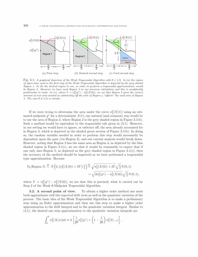
Fig. 3.1: A graphical depiction of the Weak Trapezoidal Algorithm with θ = 1/2. In (a) the regionof space-time used in the first step of the Weak Trapezoidal Algorithm is depicted by the grey shadedRegion 1. In (b) the desired region to use, in order to perform a trapezoidal approximation, wouldbe Region 2. However we have used Region 3 in our previous calculation and this is analyticallyproblematic to undo. In (c), where V = σ2

k(y∗) − σ2

k(X(0)), we see that Region 5 gives the correctamount of new area wanted as subtracting off the area of Region 4 “offsets” the used area of Region3. The case θ 6= 1/2 is similar.

If we were trying to determine the area under the curve σ2k(X(t)) using an esti-

mated midpoint y∗ for a deterministic X(t), one natural (and common) way would beto use the area of Region 2, where Region 2 is the grey shaded region in Figure 3.1(b).Such a method would be equivalent to the trapezoidal rule given in (3.1). However,in our setting we would have to ignore, or subtract off, the area already accounted forin Region 3, which is depicted as the shaded green section of Figure 3.1(b). In doingso, the random variable needed in order to perform this step would necessarily bedependent upon the past (via Region 3), and our current analysis would break down.However, noting that Region 3 has the same area as Region 4, as depicted by the blueshaded region in Figure 3.1(c), we see that it would be reasonable to expect that ifone only uses Region 5, as depicted as the grey shaded region in Figure 3.1(c), thenthe accuracy of the method should be improved as we have performed a trapezoidaltype approximation. Because

Yk(Region 5)D= N

(

0,(

σ2k(X(0)) + 2V

)

h2

)

D=

√

σ2k(X(0)) + 2V

√

h2N(0, 1)

=√

2σ2k(y

∗)− σ2k(X(0))

√

h2N(0, 1),

where V = σ2k(y

∗) − σ2k(X(0)), we see that this is precisely what is carried out by

Step 2 of the Weak θ-Midpoint Trapezoidal Algorithm.

3.2. A second point of view. To obtain a higher order method one mustboth approximate well the expected drift term as well as the quadratic variation of theprocess. The basic idea of the Weak Trapezoidal Algorithm is to make a preliminarystep using an Euler approximation and then use this step to make a higher orderapproximation to the drift integral and to the quadratic variation integral. Similar to(3.1), the desired one step approximation to the quadratic variation integrals are

∫ h

0

σ2k(X(s))ds ≈ h

[

1

2θσ2k(y

∗) +

(

1− 1

2θ

)

σ2k(Yi−1)

]

,


where all notation is as before.Considering just the variance terms of the quadratic variation, we let ei be an

orthonormal basis and see that our method yields the approximation

Var(X(h) · ei) ≈M∑

k=1

Var(

σk(Y0)(νk · ei)η1k√θh

+

√

[

α1σ2k(y

∗)− α2σ2k(Y0)

]+(νk · ei)η2k

√

(1− θ)h)

=M∑

k=1

E

(

σ2k(Y0)θ +

[

α1σ2k(y

∗)− α2σ2k(Y0)

]+(1− θ)

)

(νk · ei)2h.

If the step-size is sufficiently small, then[

α1σ2k(y

∗)−α2σ2k(Y0)

]+is positive with high

probability because of our uniform ellipticity assumption; hence,

Var(X(h) · ei) ≈ E

M∑

k=1

(νk · ei)2( 1

2θσ2k(y

∗) +(

1− 1

2θ

)

σ2k(Yi−1)

)

h,

which is a locally third order approximation to the true quadratic variation integralof

Var(X(h) · ei) = E

M∑

k=1

(νk · ei)2∫ h

0

σ2k(X(s))ds.

Notice that it was important in this simple analysis that the direction of variationνk stayed constant over the interval so that the two terms could combine exactly. Ofcourse, one should really be computing the full quadratic variation, including termssuch as Cov(X(h) · ei, X(h) · ej), but they follow the same pattern as above because

each is a linear combination of the integral terms∫ h

0σ2k(X(s))ds.

4. Proof of local error estimate

We now give the proof of the local error estimate given in Theorem 2.3 which isthe central result of this paper.

Proof. (of Theorem 2.3) We need to show that there exists a constant K so thatfor any f ∈ C6 one has

|Ef(Y1)− Ef(X(h))| ≤ K‖f‖6h3.

Hence for the reminder of the proof we fix an arbitrary f ∈ C6. Observe that Step1 of the Weak Trapezoidal Algorithm produces a value, y∗, that is distributionallyequivalent to y(θh), where y(t) solves

dy(t) = b(y(0))dt+M∑

k=1

σk(y(0)) νk dWk(t),

y(0) = x0. (4.1)

Likewise, Step 2 of the Weak Trapezoidal Algorithm produces a value, Y1, that isdistributionally equivalent to y(h), where y(t) solves

dy(t) = (α1b(y∗)− α2b(x0))dt+

M∑

k=1

√

[α1σ2k(y

∗)− α2σ2k(x0)]+ νk dWk(t),

y(θh) = y∗. (4.2)


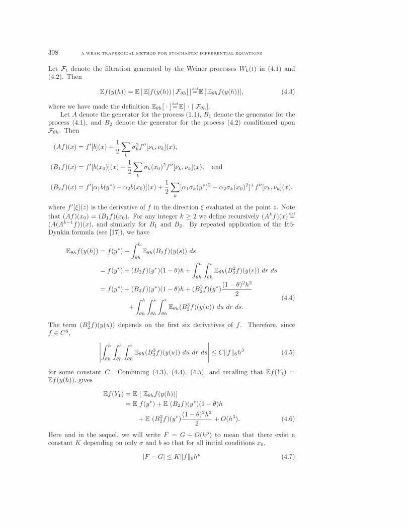
Let Ft denote the filtration generated by the Weiner processes Wk(t) in (4.1) and(4.2). Then

Ef(y(h)) = E [E[f(y(h)) | Fθh] ]def=E [Eθhf(y(h))], (4.3)

where we have made the definition Eθh[ · ]def=E[ · | Fθh].Let A denote the generator for the process (1.1), B1 denote the generator for the

process (4.1), and B2 denote the generator for the process (4.2) conditioned uponFθh. Then

(Af)(x) = f ′[b](x) +1

2

∑

k

σ2kf

′′[νk, νk](x),

(B1f)(x) = f ′[b(x0)](x) +1

2

∑

k

σk(x0)2f ′′[νk, νk](x), and

(B2f)(x) = f ′[α1b(y∗)− α2b(x0)](x) +

1

2

∑

k

[α1σk(y∗)2 − α2σk(x0)

2]+f ′′[νk, νk](x),

where f ′[ξ](z) is the derivative of f in the direction ξ evaluated at the point z. Note

that (Af)(x0) = (B1f)(x0). For any integer k ≥ 2 we define recursively (Akf)(x)def=

(A(Ak−1f))(x), and similarly for B1 and B2. By repeated application of the Ito-Dynkin formula (see [17]), we have

Eθhf(y(h)) = f(y∗) +

∫ h

θh

Eθh(B2f)(y(s)) ds

= f(y∗) + (B2f)(y∗)(1− θ)h+

∫ h

θh

∫ s

θh

Eθh(B22f)(y(r)) dr ds

= f(y∗) + (B2f)(y∗)(1− θ)h+ (B2

2f)(y∗)(1− θ)2h2

2

+

∫ h

θh

∫ s

θh

∫ r

θh

Eθh(B32f)(y(u)) du dr ds.

(4.4)

The term (B32f)(y(u)) depends on the first six derivatives of f . Therefore, since

f ∈ C6,∣

∣

∣

∣

∣

∫ h

θh

∫ s

θh

∫ r

θh

Eθh(B32f)(y(u)) du dr ds

∣

∣

∣

∣

∣

≤ C‖f‖6h3 (4.5)

for some constant C. Combining (4.3), (4.4), (4.5), and recalling that Ef(Y1) =Ef(y(h)), gives

Ef(Y1) = E [ Eθhf(y(h))]

= E f(y∗) + E (B2f)(y∗)(1− θ)h

+ E (B22f)(y

∗)(1− θ)2h2

2+O(h3). (4.6)

Here and in the sequel, we will write F = G + O(hp) to mean that there exist aconstant K depending on only σ and b so that for all initial conditions x0,

|F −G| ≤ K‖f‖6hp (4.7)


for h sufficiently small. In the spirit of the preceding calculation, repeated applicationof the Ito-Dynkin formula to (1.1) produces

Ef(X(h)) = f(x0) + (Af)(x0)h+ (A2f)(x0)h2

2+O(h3).

The proof of the theorem is then completed by Lemma 4.1 given below. Its proof,which is straightforward but tedious, is given in the appendix.

Lemma 4.1. Under the assumptions of Theorem 2.3, for all h > 0 sufficiently small

and f ∈ C6 one has

E

[

f(y∗) + (B2f)(y∗)(1− θ)h+ (B2

2f)(y∗)(1− θ)2h2

2

]

=f(x0) + (Af)(x0) + (A2f)(x0)h2

2+O(h3).

Remark 4.2. Comparing Equation (3.2) and Lemma 4.1 shows that our algorithmcan be viewed as providing an approximation to the two step Taylor series approxi-mation.

5. Examples

We present two examples that demonstrate the rate of convergence of the WeakTrapezoidal Algorithm with θ = 1/2. In each example we shall compare the accuracyof the proposed algorithm to that of Euler’s method and a “midpoint drift” algorithmdefined via repetition of the following steps

y∗ = Yi−1 + b(Yi−1)h

2,

Yi = Yi−1 + b(y∗)h+M∑

k=1

σk(Yi−1)νk ηk√h,

(5.1)

where the notation is as before. We compare the proposed algorithm to that given via(5.1) to point out that the gain in efficiency being demonstrated is not solely due tothe fact that we are getting better approximations to the drift terms, but also becauseof the superior approximation of the diffusion terms.

5.1. First example. Consider the system[

dX1(t)dX2(t)

]

=

[

X1(t)0

]

+X1(t)

[

01

]

dW1(t) +1

10

[

11

]

dW2(t), (5.2)

where W1(t) and W2(t) are standard Weiner processes. In our notation b1(x) = x1,b2(x) = 0, σ1(x) = x1, σ2(x) = 1/10, and ν1 = [0, 1]T , ν2 = [1, 1]T . Note that thenoise does not commute. It is an exercise to show that

EX2(t)2 = E X2(0)

2 − 1

2E X1(0)

2 +1

400e2t(200EX1(0)

2 + 1) +t

200− 1

400. (5.3)

For both Euler’s method and the midpoint drift method (5.1) we used step sizeshk = 1/3k, k ∈ 1, 2, 3, 4, 5 and initial condition X1(0) = X2(0) = 1 to generate500, 000 sample paths of the system (5.2). We then computed

errork(t) = EX2(t)2 − 1

5× 105

5×105∑

i=1

Xhk

2 (t)2, (5.4)


where Xhk(t) is the sample path generated numerically and EX2(t)

2 is given via (5.3).We also generated 10, 000, 000 sample paths using the Weak Trapezoidal Algorithmwith the same initial condition and step sizes hk = 1/(4k), k ∈ 1, 2, 3, 4. We thencomputed errork(t) similarly to before. The outcome of the numerical experiment issummarized in Figure 5.1a where we have plotted log(hk) versus log(|errork(1)|) forthe different algorithms. As expected, we see that the Weak Trapezoidal Algorithmgives an error that decreases proportional to h2, whereas the other two algorithmsgive errors that decrease proportional to h.

!6 !5 !4 !3 !2 !1!6

!5

!4

!3

!2

!1

0

1

log h

log error

Weak Trapezoidal

Euler

Midpoint drift

(a) First Example

!3 !2.5 !2 !1.5 !1 !0.5!5

!4

!3

!2

!1

0

1

2

log h

log error

Weak Trapezoidal

Euler

Midpoint drift

(b) Second Example

Fig. 5.1: Log-log plots of the step-size versus the error for the three different algorithms. In (a)the example (5.2) is considered. The best fit lines for the data (shown) have slopes 2.029, .998,and 1.030, for the Weak Trapezoidal Algorithm, Euler’s method, and the midpoint drift method,respectively. In (b) the example in (5.5) is considered. The best fit lines for the data (shown)have slopes 2.223, .952, and 1.098, for the Weak Trapezoidal Algorithm, Euler’s method, and themidpoint drift method, respectively. In both examples all results agree with what was expected.

5.2. Second example. Now consider the following system that is similar toone considered in [20]:

[

dX1(t)dX2(t)

]

=

[

−X2(t)X1(t)

]

+

√

sin2(X1(t) +X2(t)) + 6

t+ 1

[

10

]

dW1(t)

+

√

cos2(X1(t) +X2(t)) + 6

t+ 1

[

01

]

dW2(t),

(5.5)

where W1(t) and W2(t) are independent Weiner processes. It is simple to show that

E|X(t)|2 = EX(0)2 + 13 log(1 + t). (5.6)

We used step sizes hk = 1/(2k), k ∈ 1, 2, . . . , 8, to generate five million approximatesample paths of the system (5.5) using each of: (a) Weak Trapezoidal Algorithm, (b)Euler’s method, and (c) the midpoint drift method (5.1). We then computed

errork(t) = E|X(t)|2 − 1

5× 106

5×106∑

i=1

|Xhk(t)|2,


where Xhk(t) is the sample path generated numerically and E|X(t)|2 is given via

(5.6). The outcome is summarized in Figure 5.1b where we have plotted log(hk)versus log(|errork(1)|) for the different algorithms. As before, we see that the WeakTrapezoidal Algorithm gives an error that decreases proportional to h2, whereas theother two algorithms give errors that decrease proportional to h.

Remark 5.1. We note that in both examples we needed to average over an extremelylarge number of computed sample paths in order to estimate errork(t) for the WeakTrapezoidal Algorithm. This is due to the fact that the increased accuracy of themethod quickly makes sampling error the dominant error.

6. The effect of varying θ

The term[

α1σ2k(y

∗)−α2σ2k(Yi−1)

]+in Step 2 of the Weak Trapezoidal Algorithm

will yield zero, and the given step will have a local error of only O(h2), if

α1σ2k(y

∗) < α2σ2k(Yi−1) ⇐⇒ σ2

k(y∗) <

α2

α1σ2k(Yi−1) = (1− 2θ + 2θ2)σ2

k(Yi−1).

We will call such a step a “degenerate” step. The function g(θ) = 1 − 2θ + 2θ2 isminimized at g(1/2) = 1/2, and g(θ) → 1 as θ → 0 or θ → 1. Therefore, as mentionedRemark 2.2, one would expect that as θ → 0 or θ → 1 more steps will be degenerate,and a decrease in accuracy, together with a bias against σk decreasing, would follow.Using a step-size of h = 1/10, we tracked the percentage of degenerate steps for thesimple system

dX(t) =√

X(t)2 + 1 dW (t), X(0) = 1, (6.1)

where W (t) is a standard Weiner process. To do so, we computed 10, 000 samplepaths over the time interval [0, 1] for each of θ = .02k, k ∈ 1, . . . , 49. The resultsare shown in Figure 6.1a where the behavior predicted above is seen. Curiously, theminimum number of rejections takes place at θ = .42. It is also worth noting that

0 0.2 0.4 0.6 0.8 10

0.1

0.2

0.3

0.4

!

% of degenerate steps

(a) % of degenerate steps vs θ

!3 !2.5 !2 !1.5 !1!5.5

!5

!4.5

!4

!3.5

!3

!2.5

!2

!1.5

log h

log errror

! = .05

! = .25

! = .50

! = .75

(b) accuracy for different θ

Fig. 6.1: (a) The number of degenerate steps for the Weak Trapezoidal Algorithm applied to (6.1)with h = 1/10 and different values of θ. (b) The log h vs log(|error|) plot is given for differentchoices of θ for the Weak Trapezoidal Algorithm applied to (5.2) where the error is defined similarlyto (5.4). The best fit lines for the data (shown) have slopes 1.865, 1.996, 2.029, and 2.033 forθ = .05, .25, .50, .75, respectively.


one can check on computer software that in the general case the coefficient of h3 forthe one-step error grows like 1/θ as θ → 0. This does not happen in the deterministiccase (3.1).

While the above considerations give some interesting insight into the effect ofvarious θ, the situation is more complex. A θ closer to one should give the methodmore stability, albeit at an expense as the rejection fraction increases as θ approachesone. It would be interesting to perform a stability analysis in the spirit of [8] to betterunderstand the effect of θ. In lieu of this, Figure 6.1b gives the result of a convergenceanalysis of the Weak Trapezoidal Algorithm applied to (5.2) with different choices ofθ. Interestingly, larger θ seem to result in smaller (and hence better) convergence rateprefactors. This seems to indicate that in at least this example stability is an issue.

The performance of the Weak Trapezoidal Algorithm as a function of θ is a topicdeserving further consideration, but combining the above shows that θ = 1/2 is areasonable first choice, though stability considerations might lead one to consider a θcloser to 1.

7. Comparison to richardson extrapolation

It is illustrative to compare the Weak Trapezoidal Algorithm to Richardson ex-trapolation, which from a certain point of view is the method in the literature that ismost similar to ours. See [20] for complete details of Richardson extrapolation in theSDE setting.

Let Zh/2(t) and Zh(t) denote approximate sample paths of (1.1) generated usingEuler’s method with step sizes of h/2 and h, respectively. For all f satisfying mildassumptions, both Ef(Zh/2(t)) and Ef(Zh(t)) will approximate Ef(X(t)) with anorder of O(h). However, Richardson extrapolation may be used and the linear com-bination 2Ef(Zh/2(t)) − Ef(Zh) will approximate Ef(X(t)) with an order of O(h2)(see [20]). Of course, taking f to be the identity shows that the linear combination2Zh/2(t)−Zh(t) gives an O(h2) approximate of the mean of the process. As Richard-son extrapolation does not compute a single path, but instead uses the statistics fromtwo to achieve a higher order of approximation for a given statistic, we will compareone step of the Weak Trapezoidal Algorithm with a step-size of h, to one step of sizeh of the process 2Zh/2(t)− Zh(t) with the clear understanding that 2Zh/2(t)− Zh(t)is only O(h) accurate for higher moments.

Recall that systems of the form (1.1) are equivalent to those driven by space-timewhite noise processes (3.3). As in Section 3.1, we consider how each method uses theareas of [0,∞)2 associated to Yk(du×ds) from (3.3) during one step. We will proceedconsidering a single k since it is sufficient to illustrate the point. For Ai ⊂ [0,∞)2, wedenote by ηAi

a normal random variable with mean 0 and variance area(Ai). Recallthat ηAi

and ηAjare independent as long as Ai ∩ Aj has Lebesgue measure zero.

Consider (7.1)(a) in which we are supposing that σ2k(X(t)) increases over a single

time-step. The change in the process Zh/2 due to this k would be νk times

ηA1+ ηA2

+ ηA3.

Similarly, the change in Zh would be νk times ηA1+ ηA2

. Therefore, the change inthe process 2Zh/2(t)− Zh(t) would be νk times

ηA1+ ηA2

+ 2ηA3.

On the other hand, the change in the process generated by the Weak TrapezoidalAlgorithm due to this k is νk times

ηA1+ ηA2

+ ηA3+ ηA4

.


σ2

k(X(0))

= σ2

k(y∗)

σ2

k(X(t))

A1 A2

A3

A4

(a) When the process increases

σ2

k(X(0))

= σ2

k(y∗)

σ2

k(X(t))

A1

A2

A3

A4

(b) When the process decreases

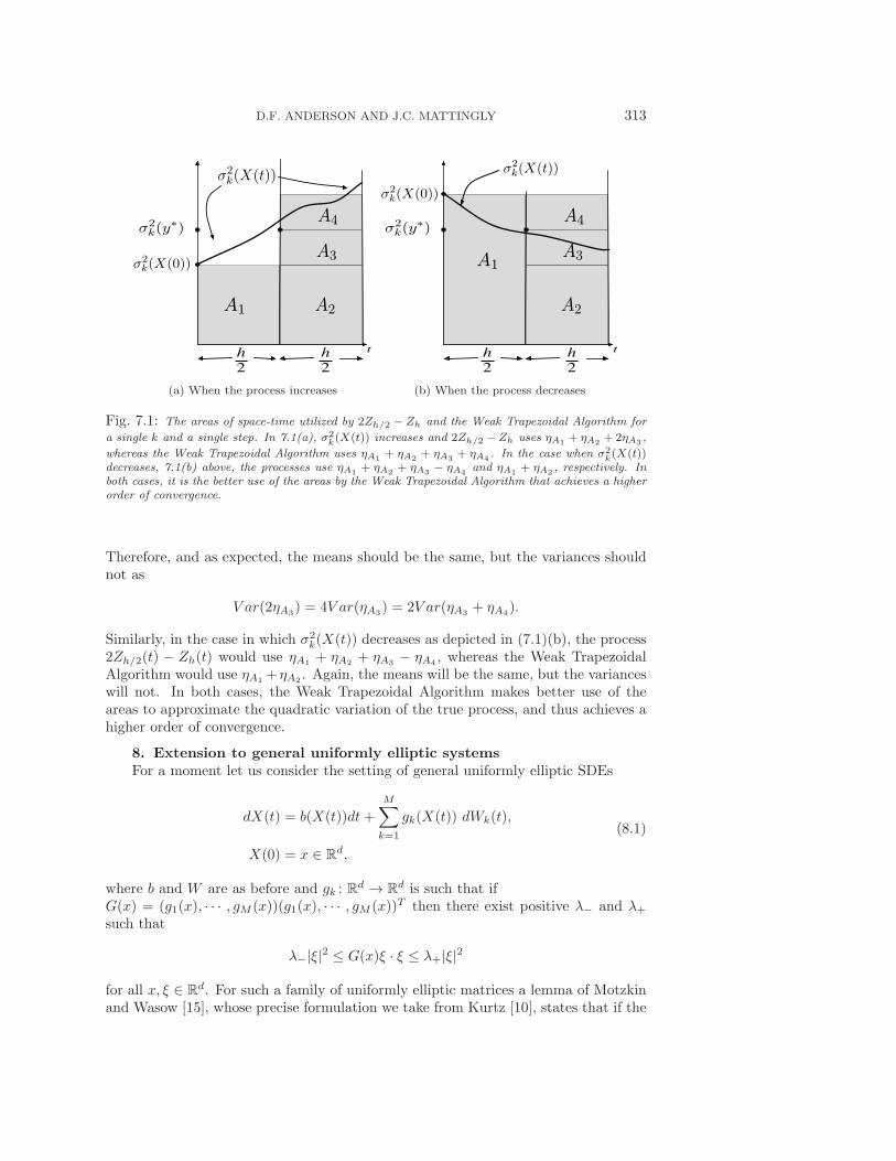
Fig. 7.1: The areas of space-time utilized by 2Zh/2 − Zh and the Weak Trapezoidal Algorithm for

a single k and a single step. In 7.1(a), σ2k(X(t)) increases and 2Zh/2 −Zh uses ηA1

+ ηA2+2ηA3

,

whereas the Weak Trapezoidal Algorithm uses ηA1+ ηA2

+ ηA3+ ηA4

. In the case when σ2k(X(t))

decreases, 7.1(b) above, the processes use ηA1+ ηA2

+ ηA3− ηA4

and ηA1+ ηA2

, respectively. Inboth cases, it is the better use of the areas by the Weak Trapezoidal Algorithm that achieves a higherorder of convergence.

Therefore, and as expected, the means should be the same, but the variances shouldnot as

V ar(2ηA3) = 4V ar(ηA3

) = 2V ar(ηA3+ ηA4

).

Similarly, in the case in which σ2k(X(t)) decreases as depicted in (7.1)(b), the process

2Zh/2(t) − Zh(t) would use ηA1+ ηA2

+ ηA3− ηA4

, whereas the Weak TrapezoidalAlgorithm would use ηA1

+ηA2. Again, the means will be the same, but the variances

will not. In both cases, the Weak Trapezoidal Algorithm makes better use of theareas to approximate the quadratic variation of the true process, and thus achieves ahigher order of convergence.

8. Extension to general uniformly elliptic systems

For a moment let us consider the setting of general uniformly elliptic SDEs

dX(t) = b(X(t))dt+

M∑

k=1

gk(X(t)) dWk(t),

X(0) = x ∈ Rd,

(8.1)

where b and W are as before and gk : Rd → R

d is such that ifG(x) = (g1(x), · · · , gM (x))(g1(x), · · · , gM (x))T then there exist positive λ− and λ+

such that

λ−|ξ|2 ≤ G(x)ξ · ξ ≤ λ+|ξ|2

for all x, ξ ∈ Rd. For such a family of uniformly elliptic matrices a lemma of Motzkin

and Wasow [15], whose precise formulation we take from Kurtz [10], states that if the


entries of G are Ck then there exists an M and σk : Rd → R≥0 : k = 1, . . . ,M,

νk ∈ Rd : k = 1, · · · ,M with σk ∈ Ck and strictly positive so that

G(x) =∑

σ2k(x)νkν

Tk .

Hence (8.1) has the same law on path space as (1.1) with these σk and νk. Of courseM might be arbitrarily large (depending on the ratio of λ+/λ−) and hence it is moresubtle to compare the total work for our method with a standard scheme based directlyon (8.1). Furthermore, depending on the dependence on x, it is not transparent howto obtain the vectors ν and functions σ exactly. Approximations could be obtainedusing the SVN of the matrix G(x) for fixed x but we do not explore this further here.

9. Conclusions and further extensions

We have presented a relatively simple method directly applicable to a wide class ofsystems which is weakly second order. We have also shown how, at least theoretically,it should be applicable to systems which do not satisfy our structural assumptionsbut are uniformly elliptic. We have picked a particularly simple setting to performour analysis to make the central points clearer. The assumption that b and σk areuniformly bounded can be relaxed to a local Lipschitz condition. That is to say,if b and σ and their needed derivatives are not bounded uniformly, but rather arebounded by an appropriate Lyapunov function, then it should be possible to extendthe method directly to the setting of unbounded coefficients provided the method isstable for the given SDE (see for instance [12]). If the SDE is not globally Lipschitzthen using an implicit drift split-step method as in [12], an adaptive method as in[11], or a truncation method as in [14] should extend to our current setting. Moreinteresting is relaxing the non-degeneracy assumption on the σk, which was used tominimize the probability of the diffusion correction being negative. This tact is insome ways reminiscent of [14] in that a modification of the method is made on a smallset of paths, though the take here is quite different. It would be interesting to use theprobability that the correction to the diffusion is negative to adapt the step-size muchin the spirit of [11]. Lastly, there is some similarity of our method with predictorcorrector methods. In the deterministic setting, predictor corrector methods not onlyhave a higher order of accuracy but also have better stability properties. There havebeen a number of papers exploring this in the stochastic context (see [5, 4, 19, 8]). Itwould be interesting to do the same with the method presented here.

Appendix A. Proof of Lemma 4.1. The proof of Lemma 4.1 requires the re-placement of the terms of the form [α1σ

2k(y

∗)−α2σ2k(x0)]

+ with [α1σ2k(y

∗)−α2σ2k(x0)].

The following two lemmas show that this can be done at the cost of an error whosesize is O(h3). Here O(h3) has the same meaning described earlier around (4.7). Webegin with an abstract technical lemma where p and q satisfy 1/p+ 1/q = 1.

Proposition A.1. Let X and Y be a real valued random variables on a probability

space (Ω,P) with |XY |Lp(Ω) < ∞ for some p ∈ (1,∞]. Then |EY [X]+ − EY X| ≤|Y X|Lp(Ω)(PX < 0)1/q. Similarly if X,Y and Z are real valued random variables

with |ZXY |Lp(Ω) < ∞ and A = X < 0 ∪ Z < 0 then |EY [X]+[Z]+ − EY XZ| ≤2|ZY X|Lp(Ω)(PA)1/q.

Proof. Let A = X < 0 and q = p/(p − 1). Then |EY ([X]+ − X)| ≤E|Y ||[X]+ − X|1A ≤ |Y X|Lp(Ω)(P(A))

1/q, showing the first claim. For the secondnotice that EY [X]+[Z]+−EY XZ = (EY [X]+Z−EY XZ)+(EY [X]+[Z]+−EY [X]+Z)and that each of the terms in parentheses can be bounded by the first result.


Corollary A.2. Let σk ∈ C2 with infx σk(x) > 0 for all k and let Y be a random

variable with |Y | ≤ C a.s. for some C. Then for any p ≥ 1 there exists an h0 so that

EY [α1σ2k(y

∗)−α2σ2k(x0)]

+ = EY [α1σ2k(y

∗)− α2σ2k(x0)] +O(hp) and

EY [α1σ2k(y

∗)−α2σ2k(x0)]

+[α1σ2ℓ (y

∗)− α2σ2ℓ (x0)]

+

=EY [α1σ2k(y

∗)− α2σ2k(x0)][α1σ

2ℓ (y

∗)− α2σ2ℓ (x0)] +O(hp)

for all h ∈ (0, h0] and k, ℓ ∈ 1, . . . ,M, where y∗ is defined via Step 1 of the Weak

Trapezoidal Algorithm.

Proof. Define the event Ak =

σk(y∗) <

α2

α1σk(x0)

. In light of Proposi-

tion A.1, it is sufficient to show that for any p > 1 there exists a Cp such thatP(Ak) ≤ Cph

p. Because σk is Lipschitz there exists a positive C such that

σ2k(x0 + δ)− α2

α1σ2k(x0) >

(

1− α2

α1

)

σ2k(x0)− C|δ|,

for any δ > 0. In particular, setting δ = y∗ − x0 = b(x0)θh +∑

j σj(x0)√θh νj η

(1)1j ,

and noting that α2 < α1 and that the σ’s are uniformly bounded from both aboveand below, the result follows from the Gaussian tails of the η’s.

Proof. (of Lemma 4.1) From Taylor’s theorem and the definition of the operatorsinvolved one has

Ef(y∗) = f(x0) + (B1f)(x0)θh+ (B21f)(x0)

θ2h2

2+O(h3)

= f(x0) + (Af)(x0)θh+ (B21f)(x0)

θ2h2

2+O(h3) .

In the last line, we have used the observation that (B1f)(x0) = (Af)(x0). Now weturn to E(B2f)(y

∗). We begin by using Lemma A.2 to remove the [ · ]+. Then we usethe fact that α1 − α2 = 1 and Taylor’s theorem to expand various terms to producethe following:

E(B2f)(y∗)

=Ef ′(y∗)[α1b(y∗)− α2b(x0)] +

1

2E

∑

k

[α1σ2k(y

∗)− α2σ2k(x0)]

+f ′′[νk, νk](y∗)

=Ef ′(y∗)[α1b(y∗)− α2b(x0)] +

1

2E

∑

k

[α1σ2k(y

∗)− α2σ2k(x0)]f

′′[νk, νk](y∗) +O(h2)

=f ′(x0)[b(x0)] +1

2

∑

k

σk(x0)2f ′′(x0)[νk, νk]

+ EB1

(

f ′[α1b− α2b(x0)] +1

2

∑

k

(α1σ2k − α2σ

2k(x0))f

′′[νk, νk])

(x0)θh+O(h2)

=(Af)(x0) + α1(B1(Af))(x0)θh− α2(B21f)(x0)θh+O(h2)

=(Af)(x0) + α1(A2f)(x0)θh− α2(B

21f)(x0)θh+O(h2).


Similar reasoning produces

E(B22f)(y

∗)

=E

(

B2

(

f ′[α1b(y∗)− α2b(x0)] +

1

2

∑

k

[α1σ2k(y

∗)− α2σ2k(x0)]

+f ′′[νk, νk])

(y∗))

=f ′′[b(x0), b(x0)](x0) + E

∑

k

[α1σ2k(y

∗)− α2σ2k(x0)]

+f ′′′[νk, νk, b(x0)](x0)

+1

4E

∑

k,j

[α1σ2k(y

∗)− α2σ2k(x0)]

+[α1σ2j (y

∗)− α2σ2j (x0)]

+f ′′′′[νk, νk, νj , νj ](x0) +O(h)

=f ′′[b(x0), b(x0)](x0) +∑

k

σ2k(x0)f

′′′[νk, νk, b(x0)](x0)

+1

4

∑

k,j

σ2k(x0)σ

2j (x0)f

′′′′[νk, νk, νj , νj ](x0) +O(h)

=(B21f)(x0) +O(h).

Combining these estimates and the fact that 2(1 − θ)θα2 = θ2 + (1 − θ)2 and 2(1 −θ)θα1 = 1 produces the quoted result after some algebra.

Appendix B. Operator bound for Pt : Ck → Ck. In this section, we show

that if b, σℓ ∈ Ck then Pt is a bounded operator from Cm to Cm for m ∈ 0, · · · , k.The k = 0 case follows immediately from |f(x)| ≤ ‖f‖0 for all x ∈ R

d. To addressthe higher k, we introduce the first k variations of Equation (1.1).

For any ξ ∈ Rd we denote the first variation of (1.1) in the direction ξ by

J (1)(t, x)[ξ] which solves the linear equation

dJ (1)(t, x)[ξ] = (∇b)(X(t))[J (1)(t, x)[ξ]] dt+

M∑

k=1

νk(∇σk)(X(t))[J (1)(t, x)[ξ]] dWk(t),

J (1)(0, x)[ξ] = ξ and X(0) = x.

Similarly for ξ = (ξ1, ξ2) ∈ R2, the second variation of X(t) (in the directions ξ) will

be denoted by J (2)(t, x)[ξ] and defined by

dJ (2)(t, x)[ξ] = (∇b)(X(t))[J (2)(t, x)[ξ]] dt+M∑

k=1

νk(∇σk)(X(t))[J (2)(t, x)[ξ]] dWk(t)

+ (∇2b)(X(t))[J (1)(t, x)[ξ1], J(1)(t, x)[ξ2]]

+

M∑

k=1

(∇2σk)(X(t))[J (1)(t, x)[ξ1], J(1)(t, x)[ξ2]]dWk(t)

J (2)(0, x)[ξ] = 0 and X(0) = x.

These equations were obtained from successive formal differentiation of (1.1).By further formal differentiation we obtain analogous equations for the k-variationJ (k)(t, x)[ξ] where ξ = (ξ1, · · · , ξk) ∈ R

k is the vector of directions. It is a standardfact that if the coefficients b, σj are in Ck then for any t > 0

supx

Ex sup

sups∈[0,t]

|J (n)(s, x)[ξ1, . . . , ξn]|p : ξi ∈ Rd with |ξi| = 1

< ∞.


This can be found in Lemma 2 in [3] on p. 196 or in a slightly different context inProposition 1.3 in [16]2 With these definitions in hand, we have that for any f ∈ C1

that

∇(Ptf)(x)[ξ] = Exf′(X(t))[J (1)(t, x)[ξ]],

∇2(Ptf)(x)[ξ] = Exf′(X(t))[J (2)(t, x)[ξ]] + Exf

(2)(X(t))[J (1)(t, x)[ξ1], J(1)(t, x)[ξ2]].

Using the moment bounds we have that for q ≥ 1 and an ever changing constant C,

E sup|ξ|=1

|∇(Ptf)(x)[ξ]|q ≤ C‖f‖qC1 sup|ξ|=1

∣

∣J(1)t [ξ]

∣

∣

q ≤ C‖f‖qC1 < ∞

E sup|ξi|=1

|∇2(Ptf)(x)[ξ1, ξ2]|q

≤ C‖f‖qC2

(

(

E sup|ξ1|=1

|J (1)(t, x)[ξ1]|2q)

12 + E sup

|ξi|=1

|J (2)(t, x)[ξ1, ξ2]]|q)

≤ C‖f‖qC2 < ∞.

Continuing in this manner we see that for any positive integer m, if f, b, σℓ ∈ Cm thenfor any q ≥ 1 one has

E sup|ξi|=1

|∇m(Ptf)(x)[ξ1, · · · , ξm]|q ≤ C‖f‖qCm < ∞

for some C. Now observe that taking q = 1 proves the desired claim on the operatornorm of Pt from Ck to Ck since

‖Ptf‖k ≤ C

k∑

j=0

E sup|ξi|=1

∣

∣(∇jPtf)(x)[ξ1, · · · , ξj ]∣

∣ ≤ C

k∑

j=0

‖f‖Cj ≤ C‖f‖Ck .

.

Acknowledgments. DFA was supported through grant NSF-DMS-0553687 andJCM through grants NSF-DMS-0449910 and NSF-DMS-06-16710 and a Sloan Foun-dation Fellowship. We would like to thank Andrew Stuart for useful comments on anearly draft and Martin Clark for stimulating questions about Richardson Extrapola-tion. We also thank Thomas Kurtz for pointing out that all uniformly elliptic SDEscan be represented in the form considered in this paper.

REFERENCES

[1] D.F. Anderson, Incorporating postleap checks in tau-leaping, J. Chem. Phys., 128, 054103, 2008.[2] D.F. Anderson, A. Ganguly and T.G. Kurtz, Error analysis of the tau-leap simulation method

for stochastically modeled chemical reaction systems, submitted.[3] D.R. Bell, The Malliavin Calculus, Pitman Monographs and Surveys in Pure and Applied

Mathematics, Longman Scientific & Technical, Harlow, 34, 1987.[4] N. Bruti-Liberati and E. Platen, Strong predictor-corrector Euler methods for stochastic dif-

ferential equations, Stoch. Dyn., 8, 561–581, 2008.[5] K. Burrage and T. Tian, Predictor-corrector methods of Runge-Kutta type for stochastic dif-

ferential equations, SIAM J. Numer. Anal., 40, 1516–1537, (electronic) 2002.[6] S.N. Ethier and T.G. Kurtz, Markov Processes: Characterization and Convergence, John Wiley

& Sons, New York, 1986.

2The statement of the Proposition demands coefficients in C∞. However the bounds on J(k)

only require Ck coefficients.


[7] J.G. Gaines and T.J. Lyons, Variable step size control in the numerical solution of stochasticdifferential equations, SIAM J. Appl. Math., 57, 1455–1484, 1997.

[8] D.J. Higham, Mean-square and asymptotic stability of the stochastic theta method, SIAM J.on Numerical Analysis, 38, 753–769, 2000.

[9] P.E. Kloeden and E. Platen, Numerical Solution of Stochastic Differential Equations, Appli-cations of Mathematics (New York), Springer-Verlag, Berlin, 23, 1992.

[10] T.G. Kurtz, Representations of markov processes as multparameter time changes, Ann. Prob.,8, 682–715, 1980.

[11] H. Lamba, J.C. Mattingly and A.M. Stuart, An adaptive Euler-Maruyama scheme for SDEs:convergence and stability, IMA J. Numer. Anal., 27, 479–506, 2007.

[12] J.C. Mattingly, A.M. Stuart and D.J. Higham, Ergodicity for SDEs and approximations: locallyLipschitz vector fields and degenerate noise, Stochastic Process. Appl., 101, 185–232, 2002.

[13] G.N. Milstein, Numerical Integration of Stochastic Differential Equations, Kluwer AcademicPress, Dordrecht, The Netherlands, 1995.

[14] G.N. Milstein and M.V. Tretyakov, Numerical integration of stochastic differential equationswith nonglobally Lipschitz coefficients, SIAM J. Numer. Anal., 43, 1139–1154, (electronic)2005.

[15] T.S. Motzkin and W. Wasow, On the approximation of linear elliptic differential equations bydifference equations with positive coefficients, J. Math. Physics, 31, 253–259, 1953.

[16] J. Norris, Simplified Malliavin calculus, in Seminaire de Probabilites, XX, 1984/85, LectureNotes in Math., Springer, Berlin, 1204, 101–130, 1986.

[17] B. Øksendal, Stochastic Differential Equations: an Introduction with Applications, Springer,Berlin, sixth ed., 2003.

[18] E. Pardoux and D. Talay, Discretization and simulation of stochastic differential equations,Acta Appl. Math., 3, 23–47, 1985.

[19] E. Platen, On weak implicit and predictor-corrector methods, Math. Comput. Simulation, 38,69–76, 1995. Probabilites numeriques Paris, 1992.

[20] D. Talay and L. Tubaro, Expansion of the global error for numerical schemes solving stochasticdifferential equations, Stochastic Analysis and Applications, 8, 483–509, 1990.

Documents

A weak trapezoidal method for a class of stochastic differential