A VARIATIONAL BAYES APPROACH TO VARIABLE SELECTION · A VARIATIONAL BAYES APPROACH TO VARIABLE SELECTION ... Bayes approximation to a linear model with a spike and ... A VARIATIONAL

Submitted to the Annals of Statistics

A VARIATIONAL BAYES APPROACH TO VARIABLE SELECTION

BY JOHN T. ORMEROD∗ , CHONG YOU∗ AND SAMUEL MULLER∗

School of Mathematics and Statistics, University of Sydney∗

We develop methodology and theory for a mean field variationalBayes approximation to a linear model with a spike and slab prioron the regression coefficients. In particular we show how our methodforces a subset of regression coefficients to be numerically indistin-guishable from zero; under mild regularity conditions estimators basedon our method consistently estimates the model parameters with eas-ily obtainable and appropriately sized standard error estimates; and,most strikingly, selects the true model at a exponential rate in the sam-ple size. We also develop a practical method for simultaneously choos-ing reasonable initial parameter values and tuning the main tuningparameter of our algorithms which is both computationally efficientand empirically performs as well or better than some popular vari-able selection approaches.

1. Introduction. Variable selection is one of the key problems in statistics as evidenced by pa-pers too numerous to mention all but a small subset. Major classes of model selection approachesinclude criteria based procedures (Akaike, 1973; Mallows, 1973; Schwarz, 1978), penalized regres-sion (Tibshirani, 1996; Fan and Li, 2001; Fan and Peng, 2004) and Bayesian modeling approaches(Bottolo and Richardson, 2010; Hans, Dobra and West, 2007; Li and Zhang, 2010; Stingo and Van-nucci, 2011). One of the key forces driving this research is model selection for large scale problemswhere the number of candidate variables is large or where the model is nonstandard in someway. Good overviews of the latest approaches to model selection are Johnstone and Titterington(2009); Fan and Lv (2010); Muller and Welsh (2010); Bulmann and van de Geer (2011); Johnsonand Rossell (2012).

Bayesian model selection approaches have the advantage of being able to easily incorporate si-multaneously many sources of variation, including prior knowledge. However, except for specialcases such as linear models with very carefully chosen priors (see for example Liang et al., 2008;or Maruyama and George, 2011), Bayesian inference via Markov chain Monte Carlo (MCMC)for moderate to large scale problems is inefficient. For this reason an enormous amount of efforthas been put into developing MCMC and similar stochastic search based methods which can beused to explore the model space efficiently (Nott and Kohn, 2005; Hans, Dobra and West, 2007;O’Hara and Sillanpaa, 2009; Bottolo and Richardson, 2010; Li and Zhang, 2010; Stingo and Van-nucci, 2011). However, for sufficiently large scale problems even these approaches can be deemedto be too slow to be used in practice. A further drawback to these methods is that there are noavailable diagnostics to determine whether the MCMC chain has either converged or explored asufficient proportion of models in the model space.

Mean field variational Bayes (VB) is an efficient but approximate alternative to MCMC forBayesian inference (Bishop, 2006; Ormerod and Wand, 2010). In general VB is typically a muchfaster, deterministic alternative to stochastic search algorithms. However, unlike MCMC, methodsbased on VB cannot achieve an arbitrary accuracy. Nevertheless, VB has shown to be an effectiveapproach to several practical problems including document retrieval (Jordan, 2004), functional

Keywords and phrases: Mean field variational Bayes, spike and slab prior, approximate Bayesian inference

1imsart-aos ver. 2014/02/20 file: VariableSelection_AnnalsFinal.tex date: June 27, 2014

2 J.T. ORMEROD ET AL.

magnetic resonance imaging (Flandin and Penny, 2007), and cluster analysis for gene-expressiondata (Teschendorff et al., 2005).

A criticism often leveled at VB methods is that they often fail to provide reliable estimates ofposterior variances. Such criticism can be made on empirical, e.g. Wand et al. (2011); Carbonettoand Stephens (2011), or theoretical grounds, e.g., Wang and Titterington (2006); Rue, Martino andChopin (2009). However, as previously shown in You, Ormerod and Muller (2014) such criticismdoes not hold for VB methods in general, at least in an asymptotic sense. Furthermore, varia-tional approximation has been shown to be useful in frequentist settings Hall, Ormerod and Wand(2011); Hall et al. (2011).

In this paper we consider a spike and slab prior on the regression coefficients (see Mitchelland Beauchamp, 1988; George and McCulloch, 1993) in order to encourage sparse estimators.This entails using VB to approximate the posterior distribution of indicator variables to selectwhich variables are to be included in the model. We consider this modification to be amongstthe simplest such modifications to the standard Bayesian linear model (using conjugate priors) toautomatically select variables to be included in the model. Our contributions are:

(i) We show how our VB method induces sparsity upon the regression coefficients;(ii) We show, under mild assumptions, that our estimators for the model parameters are consis-

tent with easily obtainable and appropriately sized standard error estimates;(iii) Under these same assumptions our VB method selects the true model at an exponential rate

in n; and(iv) We develop a practical method for simultaneously choosing reasonable initial parameter

values and tuning the main tuning parameter of our algorithms.

Contribution (iii) is a remarkable result as we do not know of another method with such a prov-ably fast rate of convergence to the true model. However, we note an important drawback of ourtheoretical analysis is that we only consider the case where n > p and p is fixed (but still possiblyvery large).

We are by no means the first to consider model selection via the use of model indicator vari-ables within the context of variational approximation. Earlier papers which use either expectationmaximization (which may be viewed as a special case of VB), or VB include Huang, Morris andFrey (2007), Rattray et al. (2009), Logsdon, Hoffman and Mezey (2010), Carbonetto and Stephens(2011), Wand and Ormerod (2011) and Rockova and George (2014). However, apart from Rockovaand George (2014), these references did not attempt to understand how sparsity was achievedand the later reference did not consider proving the rates of convergence for the estimators theyconsidered. Furthermore, each of these papers considered slightly different models and tuningparameter selection approaches to those here.

The spike and slab prior is a “sparsity inducing prior” since it has a discontinuous derivative atthe origin (owing to the spike at zero). We could also employ other such priors on our regressioncoefficients. A deluge of such papers have recently considered such priors including Polson andScott (2010), Carvalho, Polson and Scott (2010), Griffin and Brown (2011), Armagan, Dunson andLee (2013) and Neville, Ormerod and Wand (2014). Such priors entail at least some shrinkage onthe regression coefficients. We believe that some coefficient shrinkage is highly likely to be bene-ficial in practice. However, we have not pursued such priors here but focus on developing theoryfor what we believe is the simplest model deviating from the linear model which incorporates asparsity inducing prior. Adapting the theory we develop for the spike and slab prior here to othersparsity inducing priors is beyond the scope of this paper.

The paper is organized as follows. Section 2 considers model selection for a linear model using

imsart-aos ver. 2014/02/20 file: VariableSelection_AnnalsFinal.tex date: June 27, 2014

A VARIATIONAL BAYES APPROACH TO VARIABLE SELECTION 3

a spike and slab prior on the regression coefficients and provides a motivating example from realdata. Section 3 summarizes our main results which are proved in Section 4. Section 5 discussesinitialization and hyperparameter selection. Numerical examples are shown in Section 6 and il-lustrate the good empirical properties of our methods. We discuss our results and conclude inSection 7. Some auxiliary material is provided in the appendix.

2. Bayesian linear model selection. Suppose that we have observed data (yi,xi), 1 ≤ i ≤ n,and hypothesize that yi

ind.∼ N(xTi β, σ2), 1 ≤ i ≤ n for some coefficients β and noise variance σ2

where xi is p-vector of predictors. When spike and slab priors and a conjugate prior is employedon β and σ2, respectively, a Bayesian version of the linear regression model can be written asfollows,

(1)y|β, σ2 ∼ N(Xβ, σ2I), σ2 ∼ Inverse-Gamma(A,B),

βj |γj ∼ γjN(0, σ2β) + (1− γj)δ0 and γj ∼ Bernoulli(ρ), j = 1, . . . , p,

where X is a n × p design matrix whose ith row is xTi (possibly including an intercept), β =(β1, . . . ,βp)

T is a p-vector of regression coefficients, Inverse-Gamma(A,B) is the inverse Gammadistribution with shape parameter A and scale parameter B, and δ0 is the degenerate distributionwith point mass at 0. The parameters σ2β , A and B are fixed prior hyperparameters, and ρ ∈ (0, 1)is also a hyperparameter which controls sparsity. Contrasting with Rockova and George (2014)we use ρ rather than σ2β as a tuning parameter to control sparsity. The selection of ρ (or σ2β for thatmatter) is particularly important and is a point which we will discuss later.

Replacing βj with γjβj for 1 ≤ j ≤ p we can recast the model as

y|β, σ2,γ ∼ N(XΓβ, σ2I), σ2 ∼ Inverse-Gamma(A,B),

βj ∼ N(0, σ2β) and γj ∼ Bernoulli(ρ), j = 1, . . . , p,

where Γ = diag(γ1, . . . , γp) which is easier to deal with using VB. In the signal processing litera-ture this is sometimes called the Bernoulli-Gaussian (Soussen et al., 2011) or binary mask modeland is closely related to `0 regularization (see Murphy, 2012, Section 13.2.2). Wand and Ormerod(2011) also considered what they call the Laplace-zero model where the normal distributed slabin the spike and slab is replaced with a Laplace distribution. Using their naming convention thismodel might also be called a normal-zero or Gaussian-zero model.

The VB approach is summarized in many places including Bishop (2006); Rue, Martino andChopin (2009); Ormerod and Wand (2010); Carbonetto and Stephens (2011); Faes, Ormerod andWand (2011); Wand et al. (2011); Murphy (2012); Pham, Ormerod and Wand (2013); Luts andOrmerod (2014); Neville, Ormerod and Wand (2014); You, Ormerod and Muller (2014). We referthe interested reader to these papers rather than summarize the approach again here. Using avariational Bayes approximation of p(β, σ2,γ|y) by

q(β, σ2,γ) = q(β)q(σ2)

p∏j=1

q(γj)

the optimal q-densities are of the form

q∗(β) is a N(µ,Σ) density, q∗(σ2) is a Inverse-Gamma(A+ n/2, s) density

and q∗(γj) is a Bernoulli(wj) density for j = 1, . . . , p,



where a necessary (but not sufficient) condition for optimality is that the following system ofequations hold:

Σ =[τ(XTX)Ω + σ−2β I

]−1=(τWXTXW + D

)−1,(2)

µ = τ(τWXTXW + D

)−1WXTy,(3)

τ =A+ n/2

s=

2A+ n

2B + ‖y‖2 − 2yTXWµ+ tr [(XTX)Ω(µµT + Σ)],(4)

ηj = λ− τ2 (µ2j + Σj,j)‖Xj‖2 + τ

[µjX

Tj y −XT

j X−jW−j(µ−jµj + Σ−j,j)]

and(5)

wj = expit(ηj)(6)

where 1 ≤ j ≤ p, λ = logit(ρ), w = (w1 . . . wp)T , W = diag(w), Ω = wwT + W (I −W) and

D = τ(XTX)W (I−W) + σ−2β I. Note that D is a diagonal matrix.Algorithm 1 below describes an iterative process for finding parameters satisfying this system

of equations via a coordinate ascent scheme. Note that we use the notation that for a generalmatrix A, Aj is the jth column of A, A−j is A with the jth column removed. Later we willwrite Ai,j to be the value the component corresponding to the ith row and jth column of A andAi,−j is vector corresponding the ith row of A with the jth component removed. The wj ’s can beinterpreted as an approximation to the posterior probability of γj = 1 given y, that is, p(γj = 1|y),and can be used for model selection purposes, that is, the posterior probability for including thejth covariate is wj and if wj > 0.5, say, we include the jth covariate in the model.

The VB approach gives rise to the lower bound

log p(y; ρ) ≥∫q(β, σ2,γ) log

p(y,β, σ2,γ)

q(β, σ2,γ)

dθ ≡ log p(y; ρ).

At the bottom of Algorithm 1 the lower bound of log p(y; ρ) simplifies to

log p(y; ρ) = p2 −

n2 log(2π)− p

2 log(σ2β) +A log(B)− log Γ(A) + log Γ(A+ n

2

)−(A+ n

2

)log(s)

+12 log |Σ| − 1

2σ2β

tr(µµT + Σ

)+

p∑j=1

[wj log

(ρwj

)+ (1− wj) log

(1−ρ1−wj

)].

Let log p(t)(y; ρ) denote the value of the lower bound at iteration t. Algorithm 1 is terminatedwhen the increase of the lower bound log-likelihood is negligible, that is,

| log p(t)(y; ρ)− log p(t−1)(y; ρ)| < ε

where ε is a small number. In our implementation we chose ε = 10−6. Note that Algorithm 1is only guaranteed to converge to a local maximizer of this lower bound. For the n < p caseAlgorithm 1 is efficiently implemented by calculating ‖y‖2, XTy and XTX only once outside themain loop of the algorithm. Then each iteration of the algorithm can be implemented with costO(p3) and storage O(p2).

To illustrate the effect of ρ on the sparsity of the VB method we consider the prostate cancerdataset originating from a study by Stamey et al. (1989). The data consists of n = 97 sampleswith variables lcavol, lweight (log prostate weight), age, lbph (log pf the amount of benignprostate hyperplasia), svi (seminal vesicle invasion), lcp (log of capsular penetration), gleason



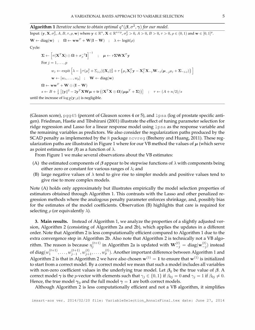
Algorithm 1 Iterative scheme to obtain optimal q∗(β, σ2,γ) for our model.Input: (y,X, σ2

β , A,B, τ, ρ,w) where y ∈ Rn, X ∈ Rn×p, σ2β > 0, A > 0, B > 0, τ > 0, ρ ∈ (0, 1) and w ∈ [0, 1]p.

W← diag(w) ; Ω← wwT + W(I−W) ; λ← logit(ρ)

Cycle:

Σ←[τ(XTX)Ω + σ−2

β I]−1

; µ← τΣWXTy

For j = 1, . . . , p

wj ← expit[λ− 1

2τ(µ2

j + Σj,j)‖Xj‖22 + τµjX

Tj y −XT

j X−jW−j(µ−jµj + Σ−j,j) ]

w← [w1, . . . , wp] ; W← diag(w)

Ω← wwT + W (I−W)

s← B + 12

[‖y‖2 − 2yTXWµ + tr

((XTXΩ)(µµT + Σ)

)]; τ ← (A+ n/2)/s

until the increase of log p(y; ρ) is negligible.

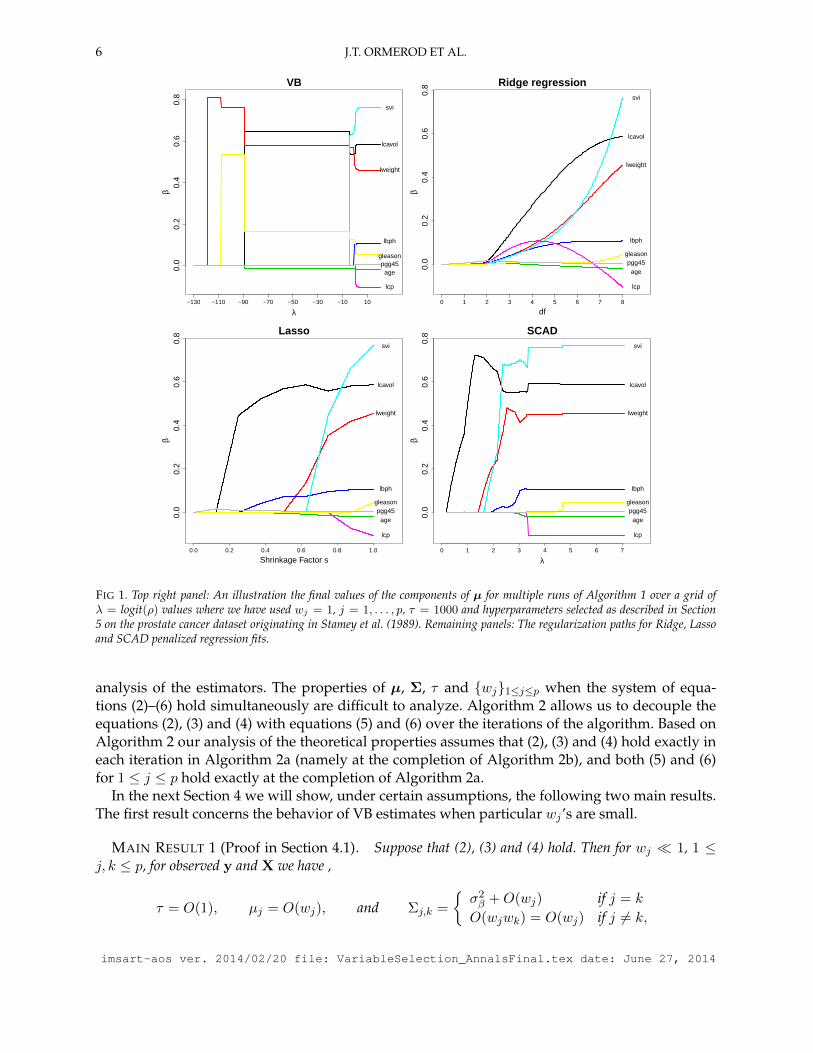
(Gleason score), pgg45 (percent of Gleason scores 4 or 5), and lpsa (log of prostate specific anti-gen). Friedman, Hastie and Tibshirani (2001) illustrate the effect of tuning parameter selection forridge regression and Lasso for a linear response model using lpsa as the response variable andthe remaining variables as predictors. We also consider the regularization paths produced by theSCAD penalty as implemented by the R package ncvreg (Breheny and Huang, 2011). These reg-ularization paths are illustrated in Figure 1 where for our VB method the values of µ (which serveas point estimates for β) as a function of λ.

From Figure 1 we make several observations about the VB estimates:

(A) the estimated components of β appear to be stepwise functions of λ with components beingeither zero or constant for various ranges of λ; and

(B) large negative values of λ tend to give rise to simpler models and positive values tend togive rise to more complex models.

Note (A) holds only approximately but illustrates empirically the model selection properties ofestimators obtained through Algorithm 1. This contrasts with the Lasso and other penalized re-gression methods where the analogous penalty parameter enforces shrinkage, and, possibly biasfor the estimates of the model coefficients. Observation (B) highlights that care is required forselecting ρ (or equivalently λ).

3. Main results. Instead of Algorithm 1, we analyze the properties of a slightly adjusted ver-sion, Algorithm 2 (consisting of Algorithm 2a and 2b), which applies the updates in a differentorder. Note that Algorithm 2 is less computationally efficient compared to Algorithm 1 due to theextra convergence step in Algorithm 2b. Also note that Algorithm 2 is technically not a VB algo-rithm. The reason is because η(t+1)

j in Algorithm 2a is updated with W(t)−j = diag(w

(t)−j) instead

of diag(w(t+1)1 , . . . , w

(t+1)j−1 , w

(t)j+1, . . . , w

(t)p ). Another important difference between Algorithm 1 and

Algorithm 2 is that in Algorithm 2 we have also chosen w(1) = 1 to ensure that w(1) is initializedto start from a correct model. By a correct model we mean that such a model includes all variableswith non-zero coefficient values in the underlying true model. Let β0 be the true value of β. Acorrect model γ is the p-vector with elements such that γj ∈ 0, 1 if β0j = 0 and γj = 1 if β0j 6= 0.Hence, the true model γ0 and the full model γ = 1 are both correct models.

Although Algorithm 2 is less computationally efficient and not a VB algorithm, it simplifies



0.0

0.2

0.4

0.6

0.8

VB

λ

β

lcavol

lweight

age

lbph

svi

lcp

gleasonpgg45

−130 −110 −90 −70 −50 −30 −10 10

0.0

0.2

0.4

0.6

0.8 Ridge regression

df

β

lcavol

lweight

age

lbph

svi

lcp

gleasonpgg45

0 1 2 3 4 5 6 7 8

0.0

0.2

0.4

0.6

0.8 Lasso

Shrinkage Factor s

β

lcavol

lweight

age

lbph

svi

lcp

gleasonpgg45

0.0 0.2 0.4 0.6 0.8 1.0

0.0

0.2

0.4

0.6

0.8 SCAD

λ

β

lcavol

lweight

age

lbph

svi

lcp

gleasonpgg45

0 1 2 3 4 5 6 7

FIG 1. Top right panel: An illustration the final values of the components of µ for multiple runs of Algorithm 1 over a grid ofλ = logit(ρ) values where we have used wj = 1, j = 1, . . . , p, τ = 1000 and hyperparameters selected as described in Section5 on the prostate cancer dataset originating in Stamey et al. (1989). Remaining panels: The regularization paths for Ridge, Lassoand SCAD penalized regression fits.

analysis of the estimators. The properties of µ, Σ, τ and wj1≤j≤p when the system of equa-tions (2)–(6) hold simultaneously are difficult to analyze. Algorithm 2 allows us to decouple theequations (2), (3) and (4) with equations (5) and (6) over the iterations of the algorithm. Based onAlgorithm 2 our analysis of the theoretical properties assumes that (2), (3) and (4) hold exactly ineach iteration in Algorithm 2a (namely at the completion of Algorithm 2b), and both (5) and (6)for 1 ≤ j ≤ p hold exactly at the completion of Algorithm 2a.

In the next Section 4 we will show, under certain assumptions, the following two main results.The first result concerns the behavior of VB estimates when particular wj ’s are small.

MAIN RESULT 1 (Proof in Section 4.1). Suppose that (2), (3) and (4) hold. Then for wj 1, 1 ≤j, k ≤ p, for observed y and X we have ,

τ = O(1), µj = O(wj), and Σj,k =

σ2β +O(wj) if j = k

O(wjwk) = O(wj) if j 6= k,



Algorithm 2a Iterative scheme to obtain optimal q∗(θ) for our model.Input: (y,X, σ2

β , A,B, τ0, ρ,w) where y ∈ Rn, X ∈ Rn×p, σ2β > 0, A > 0, B > 0, τ0 > 0, ρ ∈ (0, 1) and w(1)= 1.

t← 1 ; λ← logit(ρ)

Cycle:

(µ(t),Σ(t), τ (t))← Output from Algorithm 2b with input(y,X, σ2

β , A,B, τ0,w(t))

; W(t) ← diag(w(t)

)For j = 1, . . . , p

η(t+1)j ← λ− 1

2τ (t)[(µ(t)j

)2+ Σ

(t)j,j

]‖Xj‖2 + τ (t)XT

j

[yµ

(t)j −X−jW

(t)−j(µ

(t)−jµ

(t)j + Σ

(t)−j,j

)]w

(t+1)j ← expit(η

(t+1)j )

w(t+1) ←[w

(t+1)1 , . . . , w

(t+1)p

]T; t← t+ 1

until the increase of log p(y; ρ) is negligible.

Algorithm 2b Iterative scheme to obtain optimal output (µ(t),Σ(t), τ (t)) in Algorithm 2a.Input: (y,X, σ2

β , A,B, τ,w) where y ∈ Rn, X ∈ Rn×p, A > 0, B > 0, σ2β > 0, τ > 0 and w ∈ [0, 1]p.

W← diag(w) ; Ω← wwT + W(I−W)

Cycle:

Σ←[τ(XTX)Ω + σ−2

β I]−1

; µ← τΣWXTy

s← B + 12

[‖y‖2 − 2yTXWµ + tr

(XTXΩ)(µµT + Σ)

]; τ ← (A+ n/2)/s

until the increase of log p(y; q) is negligible

Output: (µ,Σ, τ)

and the update for w(t+1)j in Algorithm 2a with small w(t)

j satisfies

(7) w(t+1)j ← expit

[λ− 1

2τ(t)‖Xj‖2σ2β +O(w

(t)j )].

LEMMA 1 (Proof in Appendix A). Let a be a real positive number, then the quantities expit(−a) =exp(−a) +O(exp(−2a)) and expit(a) = 1− exp(−a) +O(exp(−2a)) as a→∞.

Remark: As a consequence of Main Result 1 and Lemma 1 we have that in Algorithm 2, if w(t)j

is small, the updated value w(t+1)j is approximately equal to exp(λ− τ (t)‖Xj‖2σ2β/2). Thus, when

σ2β is sufficiently large, w(t+1)j is, for numerical purposes, identically 0. This explains why that

Algorithms 1 and 2 provide sparse estimates of w and β. Furthermore, all successive values ofw(t)j

remain either small or numerically zero and may be removed safely from the algorithm reducingthe computational cost of the algorithm.

In order to establish various asymptotic properties in Main Result 2, we use the following as-sumptions (which are similar to those used in You, Ormerod and Muller, 2014) and treat yi and xias random quantities (only) in Main Result 2 and the proof of Main Result 2 in Section 4.2:

(A1) for 1 ≤ i ≤ n the yi|xi = xTi β0 + εi where εiind.∼ N(0, σ20), 0 < σ20 <∞, β0 are the true values

of β and σ2 with β0 being element-wise finite;(A2) for 1 ≤ i ≤ n the random variables xi ∈ Rp are independent and identically distributed with

p fixed;



(A3) the p×pmatrix S ≡ E(xixTi ) is element-wise finite and X = [X1, . . . ,Xp] where rank(X) = p;

and(A4) for 1 ≤ i ≤ n the random variables xi and εi are independent.

We view these as mild regularity conditions on the yi’s, εi’s and the distribution of the covariates.Note that Assumption (A3) implicitly assumes that n ≥ p. In addition to these we will assume:

(A5) for 1 ≤ j, k ≤ p the Var(xjxk) <∞;(A6) the equations (2), (3) and (4) hold when µ, Σ and τ are replaced with µ(t), Σ(t) and τ (t)

respectively; and(A7) λ ≡ λn varies with n, ρn ≡ expit(λn) and satisfies λn/n→ 0 and nρn → 0 as n→∞.

Assumption (A5) and (A6) will simplify later arguments, whereas Assumption (A7) is necessaryfor our method to identify the true model, which we will denote γ0.

We now define some notation to simplify later proofs. For an indicator vector γ the square ma-trix Wγ (W−γ) is the principal submatrix of W by distinguishing (removing) rows and columnsspecified in γ. The matrix Dγ (D−γ) is defined in the same manner. The matrix Xγ (X−γ) is thesubmatrix of X by distinguishing (removing) columns specified in γ. For example, suppose thematrix X has 4 columns, γ = (1, 0, 0, 1)T then Xγ is constructed using the first and forth columnsof X and Wγ is the submatrix of W consisting first and forth rows, and first and forth columnsof W. Similar notation, when indexing through a vector of indices v, for example, if v = (1, 4),then Xv is constructed using the first and the forth column of X and Wv is the submatrix of Wconsisting of the first and forth rows, and the first and forth columns of W. We rely on context tospecify which notation is used. We denote Ov

p(·) be a vector where each entry is Op(·), Omp (·) be

a matrix where each entry is Op(·) and Odp(·) be a diagonal matrix where diagonal elements are

Op(·). We use similar notation for op(·) matrices and vectors.

MAIN RESULT 2 (Proof in Section 4.2). If w(1)j = 1 for 1 ≤ j ≤ p and assumptions (A1)-(A6) hold

then

(8) µ(1) = β0 + Ovp

(n−1/2

), Σ(1) =

σ20n

[E(xix

Ti )]−1

+ Omp

(n−3/2

), τ (1) = σ−20 +Op

(n−1/2

)and for 1 ≤ j ≤ p we have

(9) w(2)j = expit

(η(2)j

)=

expit

[λn + n

2σ20E(x2j )β

20j +Op

(n1/2

)]j ∈ γ0,

expit [λn +Op(1)] j /∈ γ0.

If, in addition to the aforementioned assumptions, Assumption (A7) holds, then for t = 2 we have

(10)

µ(2)γ0

= β0,γ0+ Ov

p(n−1/2), µ

(2)−γ0

= Ovp(n exp(λn)),

Σ(2)γ0,γ0

=σ20n

[E(xix

Ti )]−1γ0,γ0

+ Omp

(n−3/2

), Σ

(2)−γ0,−γ0

= σ2βI + Omp (n exp(λn))

and Σ(2)γ0,−γ0

= Omp (exp(λn)),

and for 1 ≤ j ≤ p we have

(11) w(3)j = expit

(η(3)j

)=

expit[λn + n

2σ20E(x2j )β

20j +Op

(n1/2

)]j ∈ γ0,

expit[λn − n

2σ20E(x2j )σ

2β +Op

(n1/2 + n2 expit(λn))

]j /∈ γ0.



For t > 2 we have(12)

µ(t)γ0

= β0,γ0+ Ov

p(n−1/2), µ

(t)−γ0

= Ovp(n exp(−n

2σ−20 E(x2j )σ

2β)),

Σ(t)γ0,γ0

=σ20n

[E(xix

Ti )]−1γ0,γ0

+ Omp

(n−3/2

),

Σ(t)−γ0,−γ0

= σ2βI + Omp (n exp(−n

2σ−20 E(x2j )σ

2β)) and Σ

(t)γ0,−γ0

= Omp (exp(−n

2σ−20 E(x2j )σ

2β))

and for 1 ≤ j ≤ p we have

(13) w(t+1)j = expit

(η(t+1)j

)=

expit[λn + n

2σ20E(x2j )β

20j +Op

(n1/2

)]j ∈ γ0,

expit[λn − n

2σ20E(x2j )σ

2β +Op

(n1/2)

]j /∈ γ0.

Remark: This result suggests, under assumptions (A1)–(A7) and in light of Lemma 1, that thevector w(t) in Algorithm 2 approaches γ0 at an exponential rate in n. We do not know of anothermethod with a provably faster rate of convergence to the true model.

4. Proofs. We begin with some preliminary results.

RESULT 1 (Proof in Appendix A). If w(t)j > 0, 1 ≤ j ≤ p, then Ω is positive definite.

Letdof(α,w) = tr

[(XTXΩ)

(XTX)Ω + αI

−1]and

(14) Udiag(ν)UT be the eigenvalue decomposition of (XTX)Ω,

where U is an orthonormal matrix and ν = [ν1, . . . , νp]T is a vector of eigenvalues of (XTX)Ω.

RESULT 2 (Proof in Appendix A). Suppose XTX is positive definite and wj ∈ (0, 1], 1 ≤ j ≤ p andα ≥ 0 then the function dof(α,w) is monotonically decreasing in α and satisfies 0 < dof(α,w) ≤ p.

The next lemma follows from Horn and Johnson (2012, Section 0.7.3):

LEMMA 2. The inverse of a real symmetric matrix can be written as[A BBT C

]−1=

[I 0

−C−1BT I

] [A 00 C−1

] [I −BC−1

0 I

](15)

=

[A −ABC−1

−C−1BT A C−1 + C−1BT ABC−1

](16)

where A =(A−BC−1BT

)−1 provided all inverses in (15) and (16) exist.

LEMMA 3 (Proof in Appendix A). Let M be a real positive definite symmetric p × p matrix, a =[a1, . . . , ap]

T be a real vector, and let the elements of the vector b = [b1, . . . , bp]T be positive. Then the

quantity aT [M + diag(b)]−1 a is a strictly decreasing function of any element of b.



RESULT 3. Suppose that (2) and (4) hold. Then

(17) τ =2A+ n− dof(τ−1σ−2β ,w)

2B + ‖y −XWµ‖2 + µT [(XTX)W (I−W)]µ.

Proof of Result 3: Substituting (2) into (4) we may rewrite τ as

τ =2A+ n

2B + ‖y −XWµ‖2 + µT [(XTX)W (I−W)]µ+ τ−1dof(τ−1σ−2β ,w).

The result then follows after rearranging.2

Remark: Note from Result 3 that the numerator in (17) may become negative when 2A+n < p andσ2β is sufficiently large. The practical implication of this is that Algorithm 1 can fail to converge inpractice in these situations. For these reasons, and to simplify our results, we only consider thecase where n > p.

The following result bounds the values that τ can take and is useful because these bounds do notdepend on µ, Σ or w.

RESULT 4. Suppose that (2), (3) and (4) hold. Then τL ≤ τ ≤ τU where

τL =2A+ n− p

2B + ‖y‖2 + yTX(XTX)−1XTyand τU =

2A+ n

2B + ‖y −X(XTX)−1XTy‖2.

Proof of Result 4: The upper bound for τ follows from Result 3 and the inequalities (a)dof(τ−1σ−2β ,w) > 0 (from Result 2); (b) ‖y−XWµ‖2 ≥ ‖y−X(XTX)−1XTy‖2 (from least squaresresults); and (c) µT [(XTX) W (I −W)]µ ≥ 0 (as (XTX) W (I −W) is clearly at leastpositive semidefinite).

To obtain a lower bound for τ first note ‖y − XWµ‖2 ≤ ‖y‖2 + ‖XWµ‖2 via the triangleinequality. Hence, using Result 2 we have

τ ≥ 2A+ n− p2B + ‖y‖2 + µT [WXTXW + (XTX)W (I−W)]µ

=2A+ n− p

2B + ‖y‖2 + µT [(XTX)Ω]µ.

Let the eigenvalue decomposition (14) hold. Then

µT [(XTX)Ω]µ

= yTXW[Udiag(ν)UT + τ−1σ−2β I

]−1Udiag(ν)UT

[Udiag(ν)UT + τ−1σ−2β I

]−1WXTy

=

p∑j=1

νj(UTWXTy)2j

(νj + τ−1σ−2β )2≤ yTXTW

[(XTX)Ω

]−1WXTy

= yTX[XTX + W−1(XTX)W (I−W)

W−1]−1XTy

≤ yTX(XTX)−1XTy

where the last line follows from Lemma 3. Combining this inequality, using the fact from Result 2that dof(τ−1σ−2β ,w) ≤ p and Result 3 obtains the lower bound on τ .

2



4.1. Proof of Main Result 1. It is clear from the numerical example in Section 2 that sparsity inthe vector µ is achieved (at least approximately). In order to understand how sparsity is achievedwe need to understand how the quantities µ, Σ and η behave when elements of the vector w aresmall. Define the n× n matrix Pj by

(18) Pj ≡ X−jW−j(W−jX

T−jX−jW−j + τ−1D−j

)−1W−jX

T−j , 1 ≤ j ≤ p;

for j 6= k, 1 ≤ j, k ≤ p we define

P(j,k) ≡ X−(j,k)W−(j,k)

(W−(j,k)X

T−(j,k)X−(j,k)W−(j,k) + τ−1D−(j,k)

)−1W−(j,k)X

T−(j,k),

and for a indicator vector γ we define

(19) Pγ ≡ X−γW−γ(W−γXT

−γX−γW−γ + τ−1D−γ)−1

W−γXT−γ .

RESULT 5. If (2) holds then

(20) Σγ,γ =(τWγXT

γXγWγ + Dγ − τWγXTγPγXγWγ

)−1(21) and Σγ,−γ = −Σγ,γWγXT

γX−γW−γ(W−γXT

−γX−γW−γ + τ−1D−γ)−1

;

for 1 ≤ j ≤ p we have

(22) Σj,j =(σ−2β + τwj‖Xj‖2 − τw2

jXTj PjXj

)−1,

(23) and Σ−j,j = −(τW−jX

T−jX−jW−j + D−j

)−1W−jX

T−jXj(τwjΣj,j);

and for j 6= k, 1 ≤ j, k ≤ p we have

(24)Σj,k = −τwjwkXT

j (I−P(j,k))Xk

/[(σ−2β + τwj‖Xj‖2 − τw2

jXTj P(j,k)Xj

)×(σ−2β + τwk‖Xk‖2 − τw2

kXTkP(j,k)Xk

)− τwjwkXT

j (I−P(j,k))Xk2].

If (2) and (3) hold then

(25) µγ = τΣγ,γWγXTγ (I−Pγ) y;

and

(26) µj =τwjX

Tj (I−Pj)y

σ−2β + τwj‖Xj‖2 − τw2jX

Tj PjXj

, 1 ≤ j ≤ p;

and if (2), (3) and (4) hold then

(27) ηj = λ+(12τ‖Xj‖2 + w−1j σ−2β

)µ2j −

(12τ‖Xj‖2 − wjτXT

j PjXj

)Σj,j , 1 ≤ j ≤ p.



Proof of Result 5: For a given indicator vector γ we can rewrite (2) as[Σγ,γ Σγ,−γΣ−γ,γ Σ−γ,−γ

]=

[τWγXT

γXγWγ + Dγ τWγXTγX−γW−γ

W−γXT−γX1Wγτ τW−γXT

−γX−γW−γ + D−γ

]−1.

Equations (20) and (21) can be obtained by applying Equation (16) in Lemma 2 and equations (22)and (23) can be obtained by letting γ = ej (where ej is the zero vector except for the value 1 in thejth entry). Similarly,

Σ1,2 =

[10

] [D(1,2) + τW(1,2)X

T(1,2)(I−P(1,2))X(1,2)W(1,2)

]−1 [ 01

]=

−τw1w2XT1

(I−P(1,2)

)X2[

τw21X

T1

(I−P(1,2)

)X1 +D1

] [τw2

2XT2

(I−P(1,2)

)X2 +D2

]−[τw1w2XT

1

(I−P(1,2)

)X2

]2= −τw1w2X

T1

(I−P(1,2)

)X2

/[(σ−2β + τw1‖X1‖2 − τw2

1XT1 P(1,2)X1

)×(σ−2β + τw2‖X2‖2 − τw2

2XT2 P(1,2)X2

)−τw1w2X

T1 (I−P(1,2))X2

2]and (24) follows after a relabeling argument. Equation (25) follows by substituting Σγ,γ and Σγ,−γinto,

µγ =[

Σγ,γ Σγ,−γ] [ τWγXT

γy

τW−γXT−γy

]and (26) follows by letting γ = ej . Lastly, rearranging (3) we find[

τWXTXW + D]µ = τWXTy

⇒ τWXTXWµ+ Dµ = τWXTy⇒ Dµ = τWXT (y −XWµ)

⇒ w−1j djµj = τXTj (y −XWµ), for 1 ≤ j ≤ p.

Hence, via a simple algebraic manipulation, ηj may be written as

(28)

ηj = λ− 12τ(µ2j + Σj,j)‖Xj‖2 − τXT

j X−jW−jΣ−j,j

+µjτXTj (y −X−jW−jµ−j −Xjwjµj) + µ2jτwj‖Xj‖2

= λ+(wj − 1

2

)τ‖Xj‖22µ2j − 1

2τ‖Xj‖2Σj,j + τXTj (y −XWµ)µj − τXT

j X−jW−jΣ−j,j

= λ+[(wj − 1

2

)τ‖Xj‖22 + w−1j Dj

]µ2j − 1

2τ‖Xj‖2Σj,j − τXTj X−jW−jΣ−j,j .

Substituting (22), (23) and (26) into (28) and simplifying gives (27).2

From Result 4 we have that τ is bounded and that (yi,xi) are observed so that all quantities aredeterministic. From Equation (26) we see that µj is clearly O(wj) as Pj does not depend on wj .Noting that limwj→0 Σj,j = σ2β follows from Equation (22) and the result for Σj,j follows after aTaylor series argument. The result Σj,k = O(wjwk), j 6= k follows from Equation (24). We can seethat the update for w(t)

j in Algorithm 2a is as stated by combining Equation (28) with the fact that

µ(t)j = O(w

(t)j ) and Σj,j = σ2β +O(w

(t)j ). This completes the proof of Main Result 1.



4.2. Proof of Main Result 2. For the remainder of this section we will assume that y and X(and consequently µ(t),Σ(t),τ (t) and w(t) for t = 0, 1, . . .) are random quantities. Note that Results1–5 are still valid, when assuming random quantities y and X. Define the following stochasticsequences:

(29) An = n−1XTX, bn = n−1XTy, cn = dof(τ (t)σ−2β ,1) and βLS = (XTX)−1XTy.

Assuming (A1)–(A4) You, Ormerod and Muller (2014) proved consistency results for Bayesianlinear models. We will need stronger results to prove consistency of the estimates correspondingto Algorithm 2. Lemma 4 will aid in obtaining these results.

LEMMA 4 (Bishop, Fienberg and Holland, 2007, Theorem 14.4.1). If Xn is a stochastic sequencewith µn = E(Xn) and σ2n = Var(Xn) <∞, then Xn − µn = Op(σn).

Hence, from Lemma 4 and assumptions (A1)–(A5) we have

(30)

An = S + Omp

(n−1/2

), A−1n = S−1 + Om

p

(n−1/2

),

‖Xj‖2 = nE(x2j ) +Op(n1/2

), ‖ε‖2 = nσ20 +Op

(n1/2

),

n−1Xε = Ovp

(n−1/2

)and bn = n−1XT (Xβ0 + ε) = Sβ0 + Ov

p

(n−1/2

).

Before we improve upon the results of You, Ormerod and Muller (2014) we need to show that τ (t)

is bounded for all t. In fact τ (t) is bounded in probability for all t as the following result shows.

RESULT 6. Assume (A1)–(A6), then for t > 0 we have τ (t) = Op(1) and 1/τ (t) = Op(1).

Proof of Result 6: Using (A6) equations (2), (3) and (4) hold and we can use Result 4 to obtainτ−1U < τ−1 < τ−1L where

τ−1L =2B + ‖y‖2 + yTX(XTX)−1XTy

2A+ n− p=

(n

2A+ n− p

)2B + ‖y‖2 + yTX(XTX)−1XTy

n.

By (A1)–(A4) and the strong law of large numbers

1n‖y‖

2 = 1n‖Xβ0 + ε‖2 = 1

nβT0 XTXβ0 + 1

n2εTXβ0 + 1n‖ε‖

2

a.s.→ βT0 Sβ0 + 2E(εi)E(xTi )β0 + E(ε2i ) = βT0 Sβ0 + σ20.

Similarly we have, 1nyTX(XTX)−1XTy = bTnA−1n bn

a.s.→ βT0 Sβ0 and hence, τ−1La.s.→ σ20 + 2βT0 Sβ0.

In a similar manner to τL we have

τ−1U =2B + ‖y −X(XTX)−1XTy‖2

2A+ n=

(n

2A+ n

)2B + ‖y −X(XTX)−1XTy‖2

n

and 1n‖y − X(XTX)−1XTy‖2 = 1

n‖y‖2 − 1

nyTX(XTX)−1XTya.s.→ σ20 . Hence, by the continuous

mapping theoremτL

a.s.→ [2βT0 Sβ0 + σ20]−1 and τUa.s.→ σ−20

so that τ is bounded almost surely between two constants. Finally, since almost sure convergenceimplies convergence in probability the result holds.

2



We will next derive some properties for correct models. Without loss of generality let the ele-ments of β be ordered such that the first 1Tγ0 elements are nonzero and the remaining elementsare zero, that is,

β0 ≡[β0,γ

β0,−γ

]=

[β0,γ

0

]where by definition β0,−γ = 0. In the following, we denote j ∈ γ if γj = 1 and j 6∈ γ if γj = 0.

In the main result we assume that w(t) is “close” to a correct model in probability (defined inResult 7). Under this assumption we prove, in the following order, that:

• µ(t) is a consistent estimator of β;• τ (t) is a consistent estimator of σ−20 ;• Σ(t) = cov(βLS) + Om

p (n−3/2); and• w(t+1) is also “close” to the true model in probability.

We can then use these results recursively to obtain similar results for the T th iteration of theAlgorithm 2a, where T > t. In the next few results we use the following quantities:(31)

T1 = T2 −T3T4, T2 = (n−1XTγXγ) (Ω

(t)γ − 11T ) + (nτ (t)σ2β)−1I,

T3 = (nτ (t)σ2β)W(t)γ (n−1XT

γX−γ)W(t)−γ [I + T5]

−1 , T4 = W(t)−γ(n−1XT

−γXγ)W(t)γ ,

T5 = (nτ (t)σ2β)(n−1XT−γX−γ)Ω

(t)−γ and t1 = (W

(t)γ − I)(n−1XT

γy)−T3W(t)−γ(n−1XT

−γy).

RESULT 7. Assume (A1)–(A6) hold. Let γ be a correct model. Suppose that w(t) is close to γ in prob-ability in the following sense

w(t)j =

1− dnj j ∈ γdnj j /∈ γ , 1 ≤ j ≤ p,

where dnj , 1 ≤ j ≤ p, is a sequences of positive random variables such that ndnj converges in probabilityto zero. Then we say such a w(t) is close to the correct model γ in probability and

T1 = Omp (n−1 + ‖dn,γ‖∞ + n‖dn,−γ‖2∞), T2 = Om

p (n−1 + ‖dn,γ‖∞), T3 = Omp (n‖dn,−γ‖∞),

T4 = Omp (‖dn,−γ‖∞), T5 = Om

p (n‖dn,−γ‖∞) and t1 = Ovp(‖dn,γ‖∞).

Proof of Result 7: Firstly,

Ω(t)γ − 11T = (w

(t)γ )(w

(t)γ )T + W

(t)γ (I−W

(t)γ )− 11T

= (1− dn,γ)(1− dn,γ)T + (I−Dn,γ)Dn,γ − 11T

= dn,γdTn,γ − 1dTn,γ − dn,γ1T + (I−Dn,γ)Dn,γ

= Omp (‖dn,γ‖∞)

where Dn,γ = diag(dn,γ). Similarly, Ω(t)−γ = Od

p(‖dn,−γ‖∞). Again, using (30) and Result 6 wehave T2 = [Sγ,γ + Om

p (n−1/2)]Odp(‖dn,γ‖∞) + Od

p(n−1) = Om

p (n−1 + ‖dn,γ‖∞). Next, using (30)and Result 6 we have

T5 = (nτ (t)σ2β)(n−1XT−γX−γ)Ω

(t)−γ

= Op(n)[S−γ,−γ + Op(n−1/2)]Om

p (‖dn,−γ‖∞)

= Omp (n‖dn,−γ‖∞).



Expanding and simplifying the above equation obtains the result for T5. Now since, using theassumption of w(t) being close to γ (in the above sense) we have n‖dn,−γ‖∞ = op(1) and soT5 = omp (1). By the continuous mapping theorem, we have (I + T5)

−1 = I + Omp (n‖dn,−γ‖∞).

Next, T4 = Dn,−γ [S−γ,γ+Omp (n−1/2)](I−Dn,γ). Expanding and simplifying the above expression

obtains the result for T4. Furthermore,

T3 = nτ (t)σ2βTT4 (I + T5)

−1 = Op(n)Omp (‖dn,−γ‖∞)[I + Om

p (n‖dn,−γ‖∞)].

Expanding and simplifying the above expression obtains the result for T3. Substituting the orderexpressions for T2, T3 and T4 in the expression for T1. Then expanding and simplifying obtainsthe result for T1. Finally, using (30) we have

t1 = (W(t)γ − I)(n−1XT

γy)−T3W(t)−γ(n−1XT

−γy)

= Omp (‖dn,γ‖∞)[Sγ,γβ0,γ + Ov

p(n−1/2)]

−Omp (n‖dn,−γ‖∞)Om

p (‖dn−γ‖∞)[S−γ,γβ0,γ + Ovp(n−1/2)]

= Ovp(‖dn,γ‖∞ + n‖dn,γ‖∞‖dn,−γ‖∞))

which simplifies to the result for t1 under the assumption that dnj = op(n−1).

2

RESULT 8. Assume (A1)–(A6) hold. If w(t) is close to a correct model γ in probability in the sense ofResult 7, then

µ(t)γ = β0,γ + Ov

p(n−1/2), µ

(t)−γ = Ov

p(n‖dn,−γ‖∞),

Σ(t)−γ,−γ = σ2βI + Om

p (n‖dn,−γ‖∞) and Σ(t)γ,−γ = Om

p (‖dn,−γ‖∞).

Proof of Result 8: Firstly, note that

(32) τ(XTX)Ω + σ−2β I = τWXTXW + D

by definition. Using equations (19), (20) and (32) we have

Σ(t)γ,γ =

(nτ (t)

)−1[(n−1XT

γXγ)Ω(t)γ + (nτ (t)σ2β)−1I−W

(t)γ (n−1XT

γX−γ)W(t)−γ

×

(n−1XT−γX−γ)Ω

(t)−γ + (nτ (t)σ2β)−1I

−1W

(t)−γ(n−1XT

−γXγ)W(t)γ

]−1=

(nτ (t)

)−1[(n−1XT

γXγ) + T1

]−1.(33)

Using equations (19), (25), (30) and (32), Result 7, and the continuous mapping theorem we have

µ(t)γ = τ (t)Σ

(t)γ,γW

(t)γ XT

γ (I−P(t)γ )y

=[(n−1XT

γXγ) + T1

]−1[W

(t)γ (n−1XT

γY)−W(t)γ (n−1XT

γX−γ)W(t)−γ

×

(n−1XT−γX−γ)Ω

(t)−γ + (nτ (t)σ2β)−1I

−1W

(t)−γ(n−1XT

−γY)]

=[(n−1XT

γXγ) + T1

]−1[(n−1XT

γY) + t1

]=[S−1γ,γ + Om

p (n−1/2 + ‖T1‖∞)][

Sγ,γβ0,γ + Ovp(n−1/2 + ‖t1‖∞)

]= β0,γ + Ov

p(n−1/2 + ‖dn,γ‖∞ + n‖dn,−γ‖2∞).



Since by assumption ‖dn‖∞ = op(n−1) we have µ(t)

γ as stated. Using equations (19), (20) and (32)again we have

Σ(t)−γ,−γ =

[σ−2β I + τ (t)(n−1XT

−γX−γ) (nΩ(t)−γ)− nT4

(n−1XT

γXγ) + T2

−1TT

4

]−1.

From Equation (30) and Result 7, we can show that (n−1XTγXγ) + T2 = Sγ,γ + Om

p (n−1/2 +‖dn,−γ‖∞) and T4 = Om

p (‖dn,−γ‖∞). Using the continuous mapping theorem we find that

τ (t)(n−1XT−γX−γ) (nΩ

(t)−γ)− nT4

[(n−1XT

γXγ) + T2

]−1TT

4

= Op(1)[S−γ,−γ + Omp (n−1/2)]Om

p (n‖dn,−γ‖∞)

−nOmp (‖dn,−γ‖∞)

[Sγ,γ + Om

p (n−1/2 + ‖dn,γ‖∞)]Omp (‖dn,−γ‖∞)

= Omp (n‖dn,−γ‖∞).

Noting that by assumption dnj = op(n−1) and applying the continuous mapping theorem, we

obtain the result for Σ(t)−γ,−γ . Next, from equations (19), (25), (30) and Result 7 we obtain

µ(t)−γ = τ (t)Σ

(t)−γ,−γ

[(nW

(t)−γ)(n−1XT

−γY)− nT4

(n−1XT

γXγ) + T2

−1W

(t)γ (n−1XT

γY)]

= Op(1)[σ2βI + Omp (n‖dn,−γ‖∞)]

[[Om

p (n‖dn,−γ‖∞)][S−γ,−γβ0,γ + Ovp(n−1/2)]

−n[Omp (‖dn,−γ‖∞)][Sγ,γ + Om

p (n−1/2 + ‖dn,γ‖∞)][I−Odp(‖dn,γ‖∞)]

×[Sγ,γβ0,γ + Ovp(n−1/2)]

]= Ov

p(n‖dn,−γ‖∞).

Lastly, using equations (19), (21), (30), Result 7 and by the assumption that dnj = op(n−1) we

obtain

Σ(t)γ,−γ = −Σ

(t)γ,γW

(t)γ XT

γX−γW(t)−γ

[XT−γX−γ Ω

(t)−γ + (τ (t)σ2β)−1I

]−1= −

[(n−1XT

γXγ) + T1

]−1σ2βT

T4 (I + T5)

−1

=[Sγ,γ + Om

p (n−1/2) + Omp (n−1 + ‖dn,−γ‖∞ + n‖dn,−γ‖2∞)

]−1Omp (‖dn,−γ‖∞)

×[I + Om

p (n‖dn,−γ‖∞)].

After expanding the above expression and dropping appropriate lower order terms the result isproved.

2


τ (t) = σ−20 +Op(n−1/2).

Proof of Result 9: Using Result 3 the value τ (t) satisfies

τ (t) =2A+ n− dof((τ (t))−1σ−2β ,w(t))

2B + ‖y −XW(t)µ(t)‖2 + (µ(t))T [(XTX)W(t) (I−W(t))]µ(t)=

1 + T12B/n+ T2 + T3



whereT1 = A/n− n−1dof((τ (t))−1σ−2β ,w(t)), T2 = n−1‖y −XW(t)µ(t)‖2

and T3 = (µ(t))T [An W(t) (I−W(t))]µ(t).

Firstly, T1 = Op(n−1) follows from Result 2 . Secondly, using y = Xβ0 + εwe have

T2 = n−1‖ε+ X(W(t)µ(t) − β0)‖2

= n−1‖ε‖2 + 2(n−1εTX)(W(t)µ(t) − β0) + (W(t)µ(t) − β0)T (n−1XTX)(W(t)µ(t) − β0).

Using Equation (30) we have n−1‖ε‖2 = σ20+Op(n−1/2) and n−1εTX = Ov

p(n−1/2) and n−1XTX =

S+Omp (n−1/2). Note that from Result 8 we haveµ(t)

γ = β0γ+Ovp(n−1/2) andµ(t)

−γ = Ovp(n‖dn,−γ‖∞).

Then µ(t) = β0 + en where en,γ = Ovp(n−1/2) and en,−γ = Ov

p(n‖dn,−γ‖∞). Lastly, by assumption

W(t)µ(t) − β0 =

[en,γ − dn,γ β0,γ − dn,γ en,γ

dn,−γ en,−γ

]=

[Ovp(‖dn,γ‖∞ + ‖en,γ‖∞)

Ovp(‖dn,−γen,−γ‖∞)

]=

[Ovp(n−1/2 + ‖dn,γ‖∞)

Ovp(n‖dn,−γ‖2∞)

].

Hence, T2 = σ20 +Op(n−1/2 + ‖dn,γ‖∞+n‖dn,−γ‖2∞). By assumption ‖dn,γ‖∞ and n‖dn,−γ‖2∞ are

of smaller order than n−1/2 so T2 = σ20 +Op(n−1/2). Next,

T3 =

p∑j=1

(n−1‖xj‖2)(w(t)j (1− w(t)

j ))(µ(t)j )2.

Using (30) we have n−1‖xj‖2 = E(x2j )+Op(n−1/2). Using the assumption forw(t)

j we havew(t)j (1−

w(t)j ) = dnj(1 − dnj) = Op(dnj) and from Result 8 we have (µ

(t)j )2 = β20j + Op(enj). Hence, T3 =

Op(‖dn‖∞) and so

τ (t) =1 +Op(n

−1)

σ20 +Op(n−1/2)= σ20 +Op(n

−1/2).2


Σ(t)γ,γ =

σ20n

S−1γ,γ + Omp (n−3/2).

Proof of Result 10: Using Equation (33), Results 7 and 9, the matrix Σ(t)γ,γ may be written as

Σ(t)γ,γ = (nτ (t))−1

[(n−1XT

γXγ) + T1

]−1where T1, T4, T5 are as defined by (31). Using similar arguments to Result 8 we have

Σ(t)γ,γ = n−1[σ−20 +Op(n

−1/2)][Sγ,γ + Om

p (n−1/2) + Omp (n−1 + ‖dn,−γ‖∞ + n‖dn,−γ‖2∞)

]−1.

The result is proved after application of the continuous mapping theorem, expanding and drop-ping appropriate lower order terms to the above expression.

2




η(t)j =

λn + n

2σ20E(x2j )β

20j +Op

(n1/2

)j ∈ γ and j ∈ γ0,

λn +Op(1) j ∈ γ and j /∈ γ0,

λn − n2σ2

0E(x2j )σ

2β +Op(n

1/2) +Op(n2‖dn,−γ‖∞) j /∈ γ.

Proof of Result 11: If equations (2), (3) and (4) hold then by Equation (27) we have

η(t)j = λn + T6 + T7 + T8 + T9,

whereT6 = 1

2τ(t)‖Xj‖2(µ(t)j )2, T7 = (w

(t)j )−1σ−2β (µ

(t)j )2,

T8 = −12τ

(t)‖Xj‖2Σ(t)j,j and T9 = w

(t)j τ (t)XT

j P(t)j XjΣ

(t)j,j .

Note T6 ≥ 0 and T7 ≥ 0. Next, using Result 8 we have that if j ∈ γ and j ∈ γ0 then (µ(t)j )2 =

(β0j+Op(n−1/2))2 = β20j+Op(n

−1/2). If j ∈ γ and j /∈ γ0 then (µ(t)j )2 = (0+Op(n

−1/2))2 = Op(n−1).

If j /∈ γ and then (µ(t)j )2 = Op(n

2‖dn,−γ‖2∞). Hence, using Result 9 and Equation (30) we have

T6 =

n2

[σ−20 +Op(n

−1/2)] [

E(x2j ) +Op(n−1/2

)] [β20j +Op(n

−1/2)]

j ∈ γ and j ∈ γ0,

n2

[σ−20 +Op(n

−1/2)] [

E(x2j ) +Op(n−1/2

)]Op(n

−1), j ∈ γ and j /∈ γ0,

n2

[σ−20 +Op(n

−1/2)] [

E(x2j ) +Op(n−1/2

)]Op(n

2‖dn, − γ‖2∞), j /∈ γ

=

n2σ−20 E(x2j )β

20j +Op(n

1/2) j ∈ γ and j ∈ γ0,

|Op(1)| j ∈ γ and j /∈ γ0,

|Op(n3‖dn,−γ‖2∞)| j /∈ γ.

For T7 we need to consider the behavior of (w(t)j )−1(µ

(t)j )2. Note when j ∈ γ we have (w

(t)j )−1 =

1 +Op(|dnj |) and this along with Equation (26) yields

T7 =

[1− |Op(dnj)|][β20j +Op(n

−1/2)]σ−2β = Op(1) j ∈ γ and j ∈ γ0,

[1− |Op(dnj)|]Op(n−1)σ−2β = Op(n−1) j ∈ γ and j /∈ γ0,

|Op(n2‖dn,−γ‖∞)| j /∈ γ.

Next, note that T8 ≤ 0 and from Result 10 we have Σ(t)γ,γ =

σ20n [Sγ,γ ]−1 + Om

p (n−3/2) = Omp (n−1)

and Σ(t)−γ,−γ = σ2βI + Om

p (n‖dn,−γ‖∞). Hence, with Result 9 and we have

T8 =

−n2

[σ−20 +Op

(n−1/2

)] [E(x2j ) +Op

(n−1/2

)]Op(n−1

)j ∈ γ,

−n2

[σ−20 +Op

(n−1/2

)] [E(x2j ) +Op

(n−1/2

)] [σ2β +Op(n‖dn,−γ‖∞)

]j /∈ γ,

=

−|Op(1)| j ∈ γ,

−n2σ−20 E(x2j )σ

2β +Op

(n1/2 + n2‖dn,−γ‖∞

)j /∈ γ.



Lastly, using Equation (18) we have

XTj P

(t)j Xj = XT

j X−jW−j(W−jX

T−jX−jW−j + τ−1D−j

)−1W−jX

T−jXj

≤ XTj X−jW−j

(W−jX

T−jX−jW−j

)−1W−jX

T−jXj

= XTj X−j

(XT−jX−j

)−1XT−jXj

= n(n−1XTj X−j)

(n−1XT

−jX−j)−1

(n−1XT−jXj)

= n[Sj,−j + Ovp(n−1/2)]

[S−j,−j + Ov

p(n−1/2)

]−1[S−j,j + Ov

p(n−1/2)]

= Op(n).

The second line follows from Lemma 3 and the other lines follow from simplifying and usingEquation (30). Hence,

T9 =

(1 + dnj) [σ−20 +Op(n

−1/2)]Op(n)Op(n−1) = Op(1) j ∈ γ,

dnj [σ−20 +Op(n

−1/2)][Op(n)][σ2βI + Omp (n‖dn,−γ‖∞)] = Op(ndnj) j /∈ γ.

Combining the expressions for T6, T7, T8 and T9 and using the assumption that dnj = op(n−1)

obtains the result.2

Remark: At this stage we can see how Assumption (A7) comes into play. When j ∈ γ and j ∈ γ0

we do not want λn to dominate nE(x2j )β20j/2σ

20 and for j /∈ γ and j ∈ γ0 we want λn to be of

larger order than any Op(1) term. Hence, presuming that (A1)–(A7) hold, updates of the formw

(t+1)j ← expit(η

(t+1)j ) will take us from a correct model to another correct model, with the jth

variable possibly set to a value close to zero and effectively “removed.”

Proof of Main Result 2: If w(1)j = 1 for 1 ≤ j ≤ p and assumptions (A1)–(A7) hold then w(1) = 1

corresponds to a correct model γ = 1 and Results 8–11 hold with the sequence dnj = 0 for1 ≤ j ≤ p where the convergence rate of ndnj being obviously satisfied. Hence, equations (8) and(9) are proved. In order to apply these theorems again for j ∈ γ0 we need

w(2)j = expit

[λn + n

2σ20E(x2j )β

20j +Op

(n1/2

)]= 1− dnj

and for j /∈ γ0 we need w(2)j = expit [λn +Op(1)] = dnj for some sequence of random variables

dnj , 1 ≤ j ≤ p satisfying ndnj converging in probability to zero. Hence,

• If λn > 0 and λn →∞ as n→∞ then w(2)j will converge in probability to 1 for 1 ≤ j ≤ p.

• If λn is Op(1) then dnj will converge to zero at a faster rate than required for j ∈ γ0, forj /∈ γ0 the value w(2)

j will be Op(1).

• If λn < 0 and λn/n → κ for some constant κ then w(2)j may not converge in probability to 1

depending on the size of κ.• If λn < 0 and λn grows at a faster rate than Op(n) then w(2)

j will converge in probability to 0for 1 ≤ j ≤ p.• If λn → −∞ and λn/n → 0 then dnj will converge to 0 for 1 ≤ j ≤ p, but for j /∈ γ0 the

sequence ndnj may not converge in probability to zero.



Thus, we require λn → −∞, λn/n→ 0 and n expit(λn) = nρn → 0. These are the conditions spec-ified by Assumption (A7). Hence, under the assumptions (A1)–(A7) then we can apply Results8–11 with γ = γ0 (the true model) to prove equations (10) and (11). We now note that the termn2 expit(λn) is op(n) or smaller by Assumption (A7). However, by Assumption (A7) this term andλn in w(3)

j with j /∈ γ0 are dominated by −nE(x2j )σ2β/2σ

20 . Thus, we have w(3)

j = 1− dnj for j ∈ γ0

and w(3)j = dnj for j /∈ γ0 where dnj are sequences of random variables with n2dnj converging in

probability to zero. Thus, after applying Results 8–11 the equations (12) and (13) are proved fort = 3. However, these results give rise to the same conditions for t = 4 as those required for t = 3.Thus, we can continue applying Results 8–11 recursively to prove the Main Result 2 for all t.

2

5. Hyperparameter Selection and Initialization. We will now briefly discuss selecting priorhyperparameters. We have used A = B = 0.01, σ2β = 10 and initially set τ = 1000. This leavesus to choose the parameter ρ = expit(λ) and the initial values for w. The theory in Section 3and 4 suggests that if we choose w = 1 and say λ ∝ −

√n and provided with enough data then

Algorithm 1 will select the correct model. However, in practice this is not an effective strategy ingeneral since Algorithm 1 may converge to a local minimum (which means w should be carefullyselected), all values of λ satisfy Assumption (A7) when n is fixed and we do not know how muchdata is sufficient for our asymptotic results to guide the choice of λ.

Rockova and George (2014) used a deterministic annealing variant of the EM algorithm pro-posed by Ueda and Nakano (1998) to avoid local maxima problems and proved to be success-ful in that context. We instead employ a simpler stepwise procedure which initially “adds” thatvariable j (by setting wj to 1 for some j) which maximizes the lower bound log p(y; ρ) withρ = expit(−0.5

√n). We then,

(I) For fixed w select the ρj = expit(λj) which maximizes the lower bound log p(y; ρj) whereλj is an equally spaced grid between −15 and 5 of 50 points.

(II) Next, for each 1 ≤ j ≤ p, calculate the lower bound log p(y; ρ) when wj is set to both 0 and 1.The value wj is set to the value which maximizes log p(y; ρ) if this value exceeds the currentlargest log p(y; ρ).

(III) Return to (I).

This procedure is more specifically described in Algorithm 3. Note that in Algorithm 3 we use thenotation w

(k)j to denote the vector w with the jth element set to k.

6. Numerical Examples. In the following three numerical examples we only consider simu-lated, but hopefully sufficiently realistic, examples in order to reliably assess the empirical qual-ities of different methods where truth is known. We start with considering a data set with fewexplanatory variables before looking at higher dimensional situations where p = 41 and n = 80and in the third example where p = 99 and n = 2118.

We use the mean square error (MSE) to measure the quality of the prediction error defined by

MSE =1

n

n∑i=1

(Xβ0 −Xβ)2i

and the F1-score to assess the quality of model selection defined to be the harmonic mean betweenprecision and recall

F1 =2× precision× recall

precision + recallwhere precision =

TP

TP + FPand recall =

TP

TP + FN,



Algorithm 3 Iterative scheme to tune ρ and select initial w for Algorithm 1Input: (y,X, σ2

β , A,B, τ) where y ∈ Rn, X ∈ Rn×p, A > 0, B > 0, σ2β > 0, wcurr = 0 and τ > 0 M = 100; P = 50;

ρ = expit(−0.5√n); L = −∞

For i = 1, . . . ,max(p, P )

For j = 1, . . . , p

Lj ← log p(y; ρ) from Algorithm 1 with input(y,X, σ2

β , A,B, τ0, ρ,w(1)j

)k ← argmax

1≤j≤pLj; If Lk > L then set L to Lk and w to w(1)k

For i = 1, . . . ,M

For j = 1, . . . , J

Lj ← log p(y; ρj) from Algorithm 1 with input(y,X, σ2

β , A,B, τ0, ρj ,w)

k ← argmax1≤j≤pLj; If Lk > L then set L to Lk and ρ to ρk

For j = 1, . . . , p

L0 ← log p(y; ρ) from Algorithm 1 with input(y,X, σ2

β , A,B, τ0, ρ,w(0)j

)L1 ← log p(y; ρ) from Algorithm 1 with input

(y,X, σ2

β , A,B, τ0, ρ,w(1)j

)k ← argmax

j∈0,1Lj; If Lk > L then set L to Lk and w to w(k)j

If L does not improve return output of Algorithm 1 with input(y,X, σ2

β , A,B, τ0, ρ,w)

with TP , FP and FN being the number of true positives, false positives and false negativesrespectively. Note that F1 is a value between 0 and 1 and higher values are being preferred. We usethis measure to prefer methods which do not select none or all of the variables. We compare theperformance of our VB method against the Lasso, SCAD and MCP penalized regression methodsusing 10-fold cross-validation to choose the tuning parameter as implemented by the R packagencvreg (Breheny and Huang, 2011). Our methods were implemented in R and all code was runon the firrst author’s laptop computer (64 bit Windows 8 Intel i7-4930MX central processing unitat 3GHz with 32GB of random access memory).

6.1. Example 1: Solid Waste Data. The following example we take from Muller and Welsh (2010)based on a simulation study using the solid waste data of Gunst and Mason (1980). The samesettings were used in Shao (1993, 1997), Wisnowski et al. (2003), and Muller and Welsh (2005). Weconsider the model

yi = β0x0i + β1x1i + β2x2i + β3x3i + β4x4i + εi,

where i = 1, . . . , 40, the errors εi are independent and identically distributed standard normalrandom variables, x0 is a column of ones, and the values for the solid waste data variables x1, x2,x3, and x4 are taken from (Shao, 1993, Table 1). Note that these explanatory variables are highlycorrelated. We consider β to be from the set

βT ∈

(2, 0, 0, 0, 0), (2, 0, 0, 4, 0), (2, 0, 0, 4, 8), (2, 9, 0, 4, 8), (2, 9, 6, 4, 8),

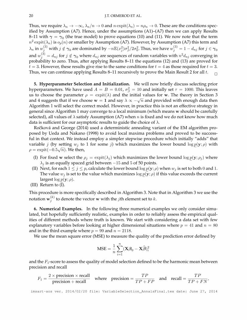
so that the number of true non-zero coefficients range from 1 to 5. Data for each of these 5 differentvalues of β were simulated 1000 times and model selection accuracy (through F1) and predictionaccuracy (through MSE) results are summarized in Figure 2.

In Figure 2 we see in the first panel that VB selects the correct model for almost every simula-tion. We also see in the second panel that VB provides smaller prediction errors when compare to



Lasso, SCAD and MCP penalty methods. All methods perform almost identically for the densecase, where the data generating model is the full model. The mean times per simulation for outVB method, and the Lasso, SCAD and MCP penalized regression methods were 0.73, 0.15, 0.17and 0.18 seconds respectively.

1 2 3 4 5

0.75

0.80

0.85

0.90

0.95

1.00

Solid WasteModel Selection Accuracy

Model size

F1

scor

e

1 2 3 4 5

−3.

5−

3.0

−2.

5−

2.0

Solid WastePrediction Accuracy

Model size

log

MS

EVBLASSOSCADMCP

FIG 2. Summaries of the model selection and prediction accuracies of VB, Lasso, SCAD and MCP methods for the Solid Wasteexample.

6.2. Example 2: Diets Simulation. We use the following example modified from Garcia et al.(2013). Let m1 and n be parameters of this simulation which are chosen to be integers. For thisexample we suppose that there are two groups of diets with n/2 subjects in each group. We gener-ate m1 + 1 explanatory variables as follows. First, we generate a binary diet indicator z where, foreach subject i = 1, . . . , n, zi = I(i > n/2)−I(i ≤ n/2). Next we generate xk = [x1,k, . . . , xn,k]

T , k =1, . . . ,m1, such that xik = uik + zivk, where uik are independent uniform (0, 1) random variables,v1, . . . , v0.75m1 are independent uniform (0.25, 0.75) random variables, and v0.75m1 + 1, . . . , vm1 areidentically zero. Thus, we have m1 variables, x1, . . . , xm1 where the first 75% of the x’s depend onz. Finally, we generate the response vector as

y = β1z + β2x1 + β3x2 + β4x3 +

m1∑k=5

βkxk−1 + βm1+1xm1 + ε,

where ε is normally distributed with mean 0 and covariance σ2I. For this simulation we set m1 =40, n = 80, σ2 = 0.5, and β = (1−κ−1/6)×(4.5, 3, 3, 3,0T , 3) where 0T is an (m1−4)-dimensionalvector of zeros and κ is a simulation parameter. The data x1, . . . ,xm1 are generated according tofour distinct categories whose interpretations are summarized in Garcia et al. (2013).

We generate 100 independent data sets for each value of κ in the set 1, 2, 3, 4 and apply eachof the variable selection procedures we consider. Note that larger values of κ in the range κ ∈ [1, 7]



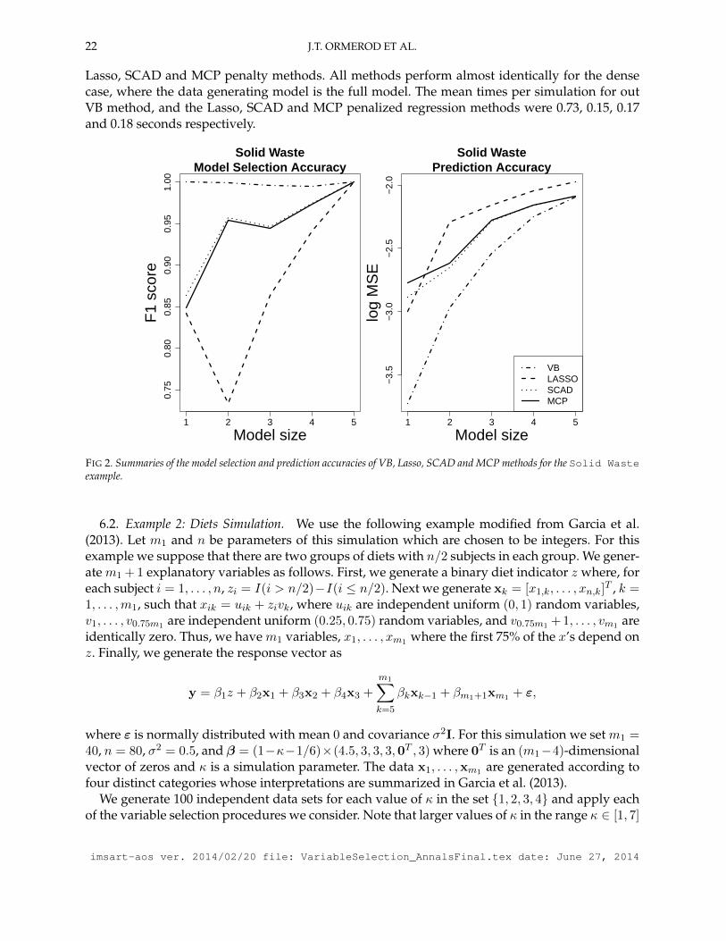
correspond to a larger signal to noise ratio. Garcia et al. (2013) considered the case where κ = 1and n = 40. The results are summarized in the last two panels of Figures 2.

In Figure 3 we see in the first panel that VB selects the correct model and in the second panelprovides smaller prediction errors for almost every simulation with the exception of κ = 4 cor-responding to the smallest signal to noise scenario. The mean times per simulation for out VBmethod, and the Lasso, SCAD and MCP penalized regression methods were 6.8, 0.4, 0.3 and 0.2seconds respectively.

1.0 1.5 2.0 2.5 3.0 3.5 4.0

0.4

0.5

0.6

0.7

0.8

0.9

1.0

Diet SimulationModel Selection Accuracy

κ

F1

scor

e

1.0 1.5 2.0 2.5 3.0 3.5 4.0

−3.

2−

3.0

−2.

8−

2.6

−2.

4−

2.2

−2.

0−

1.8

Diet SimulationPrediction Accuracy

κ

log

MS

E

VBLASSOSCADMCP

FIG 3. Summaries of the model selection and prediction accuracies of VB, Lasso, SCAD and MCP methods for the DietSimulation example.

6.3. Example 3: Communities and Crime Data. We use the Communities and Crime datasetobtained from the UCI Machine Learning Repository (http://archive.ics.uci.edu/ml/datasets/Communities+and+Crime). The data collected was part of a study by Redmondand Baveja (2002) combining socio-economic data from the 1990 United States Census, law en-forcement data from the 1990 United States Law Enforcement Management and AdministrativeStatistics survey, and crime data from the 1995 Federal Bureau of Investigation’s Uniform CrimeReports.

The raw data consists of 2215 samples of 147 variables the first 5 of which we regard as non-predictive, the next 124 are regarded as potential covariates while the last 18 variables are re-garded as potential response variables. Roughly 15% of the data is missing. We proceed with acomplete case analysis of the data. We first remove any potential covariates which contained miss-ing values leaving 101 covariates. We also remove the variables rentLowQ and medGrossRentsince these variables appeared to be nearly linear combinations of the remaining variables (thematrix X had two singular values approximately 10−9 when these variables were included). Weuse the nonViolPerPop variable as the response. We then remove any remaining samples wherethe response is missing. The remaining dataset consist of 2118 samples and 99 covariates. Finally,the response and covariates are standardized to have mean 0 and standard deviation 1.



For this data we use the following procedure as the basis for simulations.

• Use the LARS algorithm to obtain the whole Lasso path and its solution vector β:

minβ

‖y −Xβ‖22 + λ‖β‖1

for all positive values of λ. The solution for β is a piecewise function of λ with a finitenumber of pieces, say J , which can be represented by the set λ(j),β(j)1≤j≤J .• For the jth element in this path:

– Let X(j) be the columns of X corresponding to the non-zero elements of β(j).

– Find the least squares fit (β(j)

LS , σ2j ) of the data (y,X(j)).

– Simulate S datasets from the model y ∼ N(X(j)β(j)

LS , σ2I) for some value σ2.

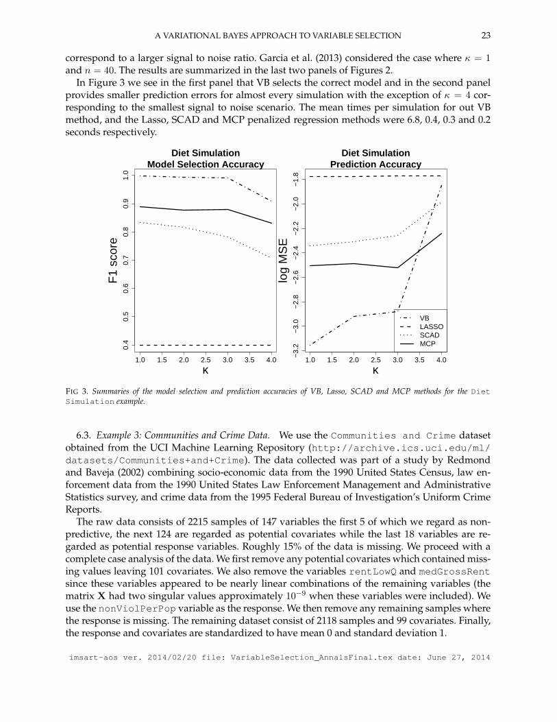
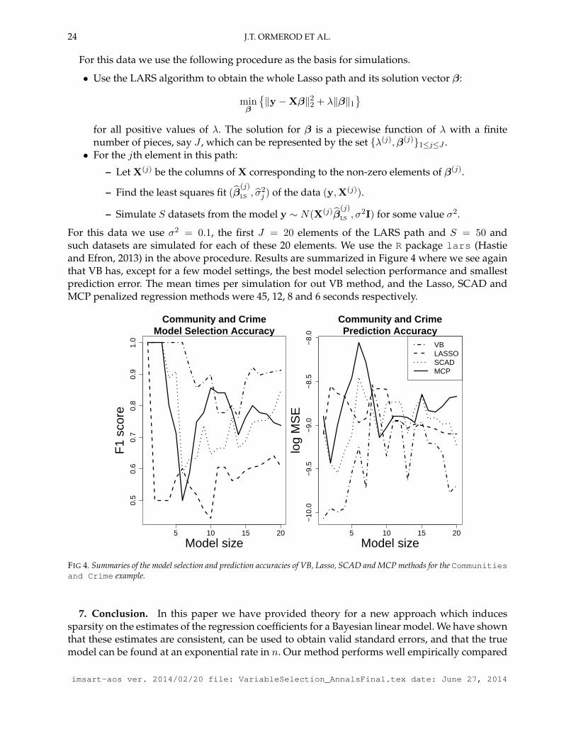
For this data we use σ2 = 0.1, the first J = 20 elements of the LARS path and S = 50 andsuch datasets are simulated for each of these 20 elements. We use the R package lars (Hastieand Efron, 2013) in the above procedure. Results are summarized in Figure 4 where we see againthat VB has, except for a few model settings, the best model selection performance and smallestprediction error. The mean times per simulation for out VB method, and the Lasso, SCAD andMCP penalized regression methods were 45, 12, 8 and 6 seconds respectively.

5 10 15 20

0.5

0.6

0.7

0.8

0.9

1.0

Community and CrimeModel Selection Accuracy

Model size

F1

scor

e

5 10 15 20

−10

.0−

9.5

−9.

0−

8.5

−8.

0

Community and CrimePrediction Accuracy

Model size

log

MS

E

VBLASSOSCADMCP

FIG 4. Summaries of the model selection and prediction accuracies of VB, Lasso, SCAD and MCP methods for the Communitiesand Crime example.

7. Conclusion. In this paper we have provided theory for a new approach which inducessparsity on the estimates of the regression coefficients for a Bayesian linear model. We have shownthat these estimates are consistent, can be used to obtain valid standard errors, and that the truemodel can be found at an exponential rate in n. Our method performs well empirically compared



to the penalized regression approaches on the numerical examples we considered. There are anumber of theoretical and methodological extensions to this work.

Theoretical extensions include considering the case where both p and n diverge. Such theorywould be important for understanding how the errors in the estimators behave as p grows rela-tive to n. A second important extension would be to analyze the effect of more elaborate shrinkagepriors on the regression coefficients, e.g., where the normal “slab” in the spike and slab is replacedby the Laplace, horseshoe, negative-exponential-gamma and generalized double Pareto distribu-tions (see for example Neville, Ormerod and Wand, 2014). Another theoretical extension includesadapting the theory presented here to non-Gaussian response.

From a practical perspective we are not completely satisfied with initialization and tuning pa-rameter selection. We do not see the approach we used here to address these issues as the mainselling point of the paper. While the result suggest that the method performs reasonably well inpractice on a number of examples, we do not believe that our approach in addressing these issuesis the best possible approach.

Perhaps the most promising practical aspect of VB methodology in practice is the potentialto handle non-standard complications. Examples of the flexibility of VB methods to handle suchcomplications are contained in Luts and Ormerod (2014). For example, it is not difficult to extendthe methodology developed here to handle elaborate response data (Wand et al., 2011), missingdata (Faes, Ormerod and Wand, 2011) or measurement error (Pham, Ormerod and Wand, 2013).This contrasts with criteria based procedures, penalized regression and some Bayesian procedures(for example Liang et al., 2008; Maruyama and George, 2011, where the models are chosen care-fully so that an exact expression for marginal likelihood is obtainable). Thus, the VB approachdeveloped here could be combined to handle these complications for powerful model selectionapproaches in these situations.

Acknowledgments. This research was partially supported by an Australian Research CouncilEarly Career Award DE130101670 (Ormerod) an Australian Research Council Discovery ProjectDP130100488 (Muller) and an Australian Postgraduate Award (You).

References.AKAIKE, H. (1973). Information theory and an extension of the maximum likelihood principle. In In Proceedings of the

2nd International Symposium on Information Theory 267–281. Akademiai Kiad6, Budapest.ARMAGAN, A., DUNSON, D. B. and LEE, J. (2013). Generalized double Pareto shrinkage. Statistica Sinica 23 119–143.BISHOP, C. M. (2006). Pattern Recognition and Machine Learning. Springer, New York.BISHOP, Y. M. M., FIENBERG, S. E. and HOLLAND, P. W. (2007). Discrete multivariate analysis: Theory and Practice.

Springer.BOTTOLO, L. and RICHARDSON, S. (2010). Evolutionary stochastic search for Bayesian model exploration. Bayesian

Analysis 5 583–618.BREHENY, P. and HUANG, J. (2011). Coordinate descent algorithms for nonconvex penalized regression, with applica-

tions to biological feature selection. The Annals of Applied Statistics 5 232–253.BULMANN, P. and VAN DE GEER, S. (2011). Statistics for High Dimensional Data. Springer.CARBONETTO, P. and STEPHENS, M. (2011). Scalable variational inference for Bayesian variable selection in regression,

and its accuracy in genetic association studies. Bayesian Analysis 6 1–42.CARVALHO, C. M., POLSON, N. G. and SCOTT, J. G. (2010). The horseshoe estimator for sparse signals. Biometrika 97

465–480.FAES, C., ORMEROD, J. T. and WAND, M. P. (2011). Variational Bayesian inference for parametric and nonparametric

regression with missing data. Journal of the American Statistical Association 106 959–971.FAN, J. and LI, R. (2001). Variable selection via onconcave penalized likelihood and its oracle properties. Journal of the

American Statistical Association 96 1348–1360.FAN, J. and LV, J. (2010). A selective overview of variable selection in high dimensional feature space. Statistica Sinica

20 101-148.



FAN, J. and PENG, H. (2004). Nonconcave penalized likelihood with a diverging number of parameters. The Annals ofStatistics 32 928–961.

FLANDIN, G. and PENNY, W. D. (2007). Bayesian fMRI data analysis with sparse spatial basis function priors. NeuroIm-age 34 1108-1125.

FRIEDMAN, J., HASTIE, T. and TIBSHIRANI, R. (2001). The Elements of Statistical Learning. Springer.GARCIA, T. P., MULLER, S., CARROLL, R. J., DUNN, T. N., THOMAS, A. P., ADAMS, S. H., PILLAI, S. D. and

WALZEM, R. L. (2013). Structured variable selection with q-values. Biostatistics 14 695–707.GEORGE, E. I. and MCCULLOCH, B. E. (1993). Variable Selection via Gibbs Sampling. Journal of the American Statistical

Association 88 1023–1032.GRIFFIN, J. and BROWN, P. (2011). Bayesian adaptive lassos with non-convex penalization. Australian New Zealand

Journal of Statistics 53 423–442.GUNST, R. F. and MASON, R. L. (1980). Regression analysis and its application: a data-oriented approach. New York: Marcel

Dekker.HALL, P., ORMEROD, J. T. and WAND, M. P. (2011). Theory of Gaussian variational approximation for a Poisson mixed

model. Statistica Sinica 21 369–389.HALL, P., PHAM, T., WAND, M. P. and WANG, S. S. J. (2011). Asymptotic normality and valid inference for Gaussian

variational approximation. The Annals of Statistics 39 2502–2532.HANS, C., DOBRA, A. and WEST, M. (2007). Shotgun stochastic search for “large p” regression. Journal of the American

Statistical Association 102 507–516.HASTIE, T. and EFRON, B. (2013). lars 1.2. Least angle regression, lasso and forward stagewise regression. R package.

http://cran.r-project.org.HORN, R. A. and JOHNSON, C. R. (2012). Matrix Analysis. Cambridge University Press.HUANG, J. C., MORRIS, Q. D. and FREY, B. J. (2007). Bayesian inference of MicroRNA targets from sequence and

expression data. Journal of Computational Biology 14 550–563.JOHNSON, V. E. and ROSSELL, D. (2012). Bayesian Model Selection in High-Dimensional Settings. Journal of the Ameri-

can Statistical Association 107 649-660.JOHNSTONE, I. M. and TITTERINGTON, D. M. (2009). Statistical challenges of high-dimensional data. Philosophical

Transactions of the Royal Society A: Mathematical, Physical and Engineering Sciences 367 4237-4253.JORDAN, M. I. (2004). Graphical Models. Statistical Science 19 140-155.LI, F. and ZHANG, N. R. (2010). Bayesian variable selection in structured high-dimensional covariate spaces with

applications in genomics. Journal of the American Statistical Association 105 1202–1214.LIANG, F., PAULO, R., MOLINA, G., CLYDE, M. A. and BERGER, J. O. (2008). Mixtures of g priors for Bayesian variable

selection. Journal of the American Statistical Association 103 410–423.LOGSDON, B. A., HOFFMAN, G. E. and MEZEY, J. G. (2010). A variational Bayes algorithm for fast and accurate mul-

tiple locus genome-wide association analysis. BMC Bioinformatics 11 1–13.LUTS, J. and ORMEROD, J. T. (2014). Mean field variational Bayesian inference for support vector machine classification.

Computational Statistics and Data Analysis 73 163–176.MALLOWS, C. L. (1973). Some comments on Cp. Technometrics 15 661–675.MARUYAMA, Y. and GEORGE, E. I. (2011). Fully Bayes factors with a generalized g-prior. The Annals of Statistics 39

2740–2765.MITCHELL, T. J. and BEAUCHAMP, J. J. (1988). Bayesian Variable Selection in Linear Regression. Journal of the American

Statistical Association 83 1023–1032.MULLER, S. and WELSH, A. H. (2005). Outlier robust model selection in linear regression. Journal of the American

Statistical Association 100 1297–1310.MULLER, S. and WELSH, A. H. (2010). On model selection curves. International Statistical Review 78 240–256.MURPHY, K. P. (2012). Machine Learning: A Probabilistic Perspective. The MIT Press, London.NEVILLE, S., ORMEROD, J. T. and WAND, M. P. (2014). Mean Field Variational Bayes for Continuous Sparse Signal

Shrinkage: Pitfalls and Remedies. Electronic Journal of Statistics.NOTT, D. J. and KOHN, R. (2005). Adaptive sampling for Bayesian variable selection. Biometrika 92 747–763.O’HARA, R. B. and SILLANPAA, M. J. (2009). A review of Bayesian variable selection methods: what, how and which.

Bayesian analysis 4 85–117.ORMEROD, J. T. and WAND, M. P. (2010). Explaining variational approximations. The American Statistician 64 140–153.PHAM, T. H., ORMEROD, J. T. and WAND, M. P. (2013). Mean field variational Bayesian inference for nonparametric

regression with measurement error. Computational Statistics and Data Analysis 68 375–387.POLSON, N. G. and SCOTT, J. G. (2010). Shrink globally, act locally: sparse Bayesian regularization and prediction. In

Bayesian Statistics 9 (J. M. BERNARDO, M. J. BAYARRI, A. P. D. J. O. BERGER, D. HECKERMAN, A. F. M. SMITH andM. WEST, eds.). Oxford University Press, Oxford.

RATTRAY, M., STEGLE, O., SHARP, K. and WINN, J. (2009). Inference algorithms and learning theory for Bayesian



sparse factor analysis. In Journal of Physics: Conference Series 197 012002.REDMOND, M. and BAVEJA, A. (2002). A data-driven software tool for enabling cooperative information sharing

among police departments. European Journal of Operational Research 141 660–678.ROCKOVA, V. and GEORGE, E. I. (2014). EMVS: The EM approach to Bayesian variable selection. Journal of the American

Statistical Association 109 828-846.RUE, H., MARTINO, S. and CHOPIN, N. (2009). Approximate Bayesian inference for latent Gaussian models by using

integrated nested Laplace approximations. Journal of the Royal Statistical Society, Series B 71 319–392. MR2649602SCHWARZ, G. (1978). Estimating the dimension of a model. The Annals of Statistics 6 461–464.SHAO, J. (1993). Linear model selection by cross-validation. Journal of the American statistical Association 88 486–494.SHAO, J. (1997). An asymptotic theory for linear model selection. Statistica Sinica 7 221–242.SOUSSEN, C., IDIER, J., BRIE, D. and DUAN, J. (2011). From Bernoulli–Gaussian deconvolution to sparse signal restora-

tion. Signal Processing, IEEE Transactions on 59 4572–4584.STAMEY, T. A., KABALIN, J. N., MCNEAL, J. E., JOHNSTONE, I. M., FREIHA, F., REDWINE, E. A. and YANG, N. (1989).

Prostate specific antigen in the diagnosis and treatment of adenocarcinoma of the prostate: II. radical prostatectomytreated patients. Journal of Urology 141 1076–1083.

STINGO, F. C. and VANNUCCI, M. (2011). Variable selection for discriminant analysis with Markov random field priorsfor the analysis of microarray data. Bioinformatics 27 495–501.

TESCHENDORFF, A. E., WANG, Y., BARBOSA-MORAIS, N. L., BRENTON, J. D. and CALDAS, C. (2005). A VariationalBayesian Mixture Modelling Framework for Cluster Analysis of Gene-Expression Data. Bioinformatics 21 3025-3033.

TIBSHIRANI, R. (1996). Regression shrinkage and selection via the lasso. Journal of the Royal Statatistical Society, Series B58 267–288.

UEDA, N. and NAKANO, R. (1998). Deterministic annealing EM algorithm. Neural Networks 11 271–282.WAND, M. P. and ORMEROD, J. T. (2011). Penalized wavelets: Embedding wavelets into semiparametric regression.

Electronic Journal of Statistics 5 1654–1717.WAND, M. P., ORMEROD, J. T., PADOAN, S. A. and FRUHWIRTH, R. (2011). Mean Field Variational Bayes for Elaborate

Distributions. Bayesian Analysis 6 847–900.WANG, B. and TITTERINGTON, D. M. (2006). Convergence properties of a general algorithm for calculating variational

Bayesian estimates for a normal mixture model. Bayesian Analysis 1 625–650.WISNOWSKI, J. W., SIMPSON, J. R., MONTGOMERY, D. C. and RUNGER, G. C. (2003). Resampling methods for variable

selection in robust regression. Computational Statistics & Data Analysis 43 341–355.YOU, C., ORMEROD, J. T. and MULLER, S. (2014). On variational Bayes estimation and variational information criteria

for linear regression models. Australian and New Zealand Journal of Statistics 56 83–87.

Appendix A: Auxiliary results.

Proof Lemma 1: Note that | expit(−a)−exp(−a)| = exp(−2a)/(1+exp(−a)) < exp(−2a), and alsonote that expit(a) = 1− expit(−a). Hence the result is as stated.

2

Proof of Result 1: A matrix is positive definite if and only if for all non-zero real vector a =[a1, . . . , ap]

T the scalar aTΩa is strictly positive (Horn and Johnson, 2012, Section 7.1). By definitionaTΩa = aT

[wwT +W(I−W)

]a = (

∑pj=1 ajwj)

2 +∑p

j=1 a2jwj(1−wj). As 0 < w

(t)j ≤ 1, 1 ≤ j ≤ p,

we have wj(1−wj) ≥ 0 and hence∑p

j=1 a2jwj(1−wj) ≥ 0. Again, as w(t)

j > 0, 1 ≤ j ≤ p, we have(∑p

j=1 ajwj)2 > 0 for any non-zero vector a. Hence, the result is as stated.

2

Proof of Result 2 : Let the eigenvalue decomposition (14) hold. Since wj ∈ (0, 1], 1 ≤ j ≤ p ispositive by Result 1 the matrix Ω is positive definite. By the Schur product theorem (Horn andJohnson, 2012, Theorem 7.5.2), the matrix (XTX) Ω is also positive definite. Hence, νi > 0,i = 1, . . . , p. Then, using properties of the orthonormal matrix U, we have

dof(α,w) = tr[Udiag(ν)UT

(Udiag(ν)UT + αI

)−1]=

p∑j=1

νjνj + α

.

Clearly, dof(α,w) is monotonically decreasing in α, dof(0,w) = p and dof(α,w) only approacheszero as α→∞.



2

Proof of Lemma 3: Let the matrix M + diag(b) be partitioned as

M + diag(b) =

[M11 + b1 mT

12

m12 M22 + B2

]where m12 = [M12, . . . ,M1p]

T , B2 = diag(b2, . . . , bp) and

M22 =

M22 · · · M2p...

. . ....

Mp2 · · · Mpp

.Then, by Equation (15) in Lemma 2,

(34) aT [M + diag(b)]−1 a =c21

b1 +M11 −mT12(M22 + B2)−1m12

+ cT2 (M22 + B2)−1c2

where

c =

[1 −mT

12(M22 + B2)−1

0 I

]a and c2 = [c2, . . . , cp]

T .

Note any principal submatrix of a positive definite matrix is positive definite (Horn and Johnson,2012, Chapter 7.1.2). Hence, the matrix (M + diag(b))−1 is positive definite and (b1 + M11 −mT

12(M22 + B2)−1m12)

−1 is a positive scalar. Clearly, (34) is strictly decreasing as b1 increases. Theresult follows for bj , 2 ≤ j ≤ p after a relabeling argument.

2

ADDRESS OF THE FIRST, SECOND AND THIRD AUTHORSSCHOOL OF MATHEMATICS AND STATISTICS, UNIVERSITY OF SYDNEY, SYDNEY 2006, AUSTRALIA

[email protected]; [email protected]; [email protected]


Documents

A VARIATIONAL BAYES APPROACH TO VARIABLE SELECTION · A VARIATIONAL BAYES APPROACH TO VARIABLE SELECTION ... Bayes approximation to a linear model with a spike and ... A VARIATIONAL