Embed Size (px)
Citation preview

A uni�ed framework for testing in the linear regression
model under unknown order of fractional integration∗
Bent Jesper Christensen†, Robinson Kruse‡ and Philipp Sibbertsen§
October 22, 2013
Abstract
We consider hypothesis testing in a general linear time series regression framework
when the possibly fractional order of integration of the error term is unknown. We
show that the approach suggested by Vogelsang (1998a) for the case of integer inte-
gration does not apply to the case of fractional integration. We propose a Lagrange
Multiplier-type test whose limiting distribution is independent of the order of inte-
gration of the errors. Di�erent testing scenarios for the case of deterministic and
stochastic regressors are considered. Simulations demonstrate that the proposed test
works well for a variety of di�erent cases, thereby emphasizing its generality.
Key words: Long memory; linear time series regression; Lagrange Multiplier test.
JEL classi�cation: C12 (Hypothesis Testing), C22 (Time-Series Models)
∗We are grateful to the participants of the Workshop on Long Memory Time Series in Aarhus, theWorkshop on Nonlinear and Persistent Time Series in Hannover, the Workshop in Honor of James David-son in Exeter, the European Meeting of Statisticians in Budapest and the ESEM in Gothenburg for helpfulcomments. We are especially grateful to Karim Abadir, Richard Baillie, Jörg Breitung, Matei Demetrescu,David Hendry and Peter Phillips for fruitful discussions. Financial support of the Deutsche Forschungs-gemeinschaft (DFG) is gratefully acknowledged. Bent Jesper Christensen and Robinson Kruse gratefullyacknowledges �nancial support from CREATES funded by the Danish National Research Foundation.Part of this research was carried out while Philipp Sibbertsen was a Guest Professor at CREATES. Theirkind hospitality is greatly appreciated.†CREATES, Aarhus University, School of Business and Social Sciences, Fuglesangs Allé 4, DK-8210
Aarhus V, Denmark and Aarhus Institute of Advanced Studies, Høegh-Guldbergs Gade 6B, DK-8000Aarhus C. E-mail address: [email protected] .‡CREATES, Aarhus University, School of Business and Social Sciences, Fuglesangs Allé 4, DK-8210
Aarhus V, Denmark. E-mail address: [email protected] . Leibniz University Hannover, School ofEconomics and Management, Institute for Statistics, Königsworther Platz 1, D-30167 Hannover, Ger-many. E-mail address: [email protected] .§Leibniz University Hannover, School of Economics and Management, Institute
for Statistics, Königsworther Platz 1, D-30167 Hannover, Germany. E-mail address:[email protected]
1
1 Introduction
This paper considers the problem of hypothesis testing in a linear regression model when
the order of possibly fractional integration of the error term is unknown. Speci�cally, we
consider the linear regression model
yt = β′zt + et,
where zt is a p× 1 vector of deterministic or stochastic (or both) regressors ful�lling some
regularity conditions speci�ed later, β is a p×1 vector of regression parameters and et is an
error term which is possibly fractionally integrated of unknown order d0, i.e. et ∼ I(d0).
In the case of stochastic regressors, their orders of integration are assumed to be the same
(d1) and unknown as well. We are concerned with testing hypotheses for β. It is well
known that the behavior of standard tests for restrictions on β strongly depend on the
order of integration of the error term. Neglecting the fractional nature of the errors leads
typically to invalid inference.
Vogelsang (1998a) suggests a testing approach which allows valid inference to be drawn
when the order of integration of the error term is unknown. The test is embedded in a
linear trend testing framework where the errors are allowed to be I(0) or I(1). Other con-
tributions cover the case of testing for location (Zambrano and Vogelsang, 2000), testing
against a mean shift (Vogelsang, 1998b) and nonlinear trends (Harvey, Leybourne and
Xiao, 2010). Regarding test against trend breaks, Harvey, Leybourne and Taylor (2009)
and Perron and Yabu (2009) suggest alternative approaches. All of the aforementioned
studies are based on having a choice of two possible orders of integration of which one
is the true order. In the fractional case we have a continuum of possible orders of inte-
gration which renders methods designed for the I(0) and I(1) case problematic. Another
important feature of these tests is that they are dealing with deterministic regressors.
In order to achieve the goal of conducting valid inference on β in linear regression
models with deterministic or stochastic regressors with I(d) errors, we suggest a Lagrange
multiplier (LM) test. The test is derived under fairly mild regularity assumptions ensuring
�exibility of our method. In a similar regression framework Robinson (1994) suggests an
LM test for the order of integration d. Thereby, our work complements Robinson (1994).
Our test exhibits a standard limiting distribution and is shown to have non-trivial power
against local alternatives. These results remain valid, when an LM-type test is carried
out where the memory parameter is estimated in a semi-parametric way, by e.g. exact
local Whittle, see Shimotsu and Phillips (2005). The reason for applying semi-parametric
estimation arises from the need of an estimator for the fractional integration parameter
which is consistent under validity of the null and the alternative hypothesis. Biased
estimation would lead to size distortions and power losses in �nite samples. To this end,
2

estimation is carried out under the alternative hypothesis. Simulation results for various
situations, i.e. linear and quadratic trends, mean shifts and trend breaks, as well as
fractional cointegration, shed light on the empirical properties of the test. The results
demonstrate that the LM-type test performs well in practice.
The problem of testing under an unknown order of possibly fractional integration
has recently been investigated elsewhere in several speci�c testing situations involving
deterministic regressors. Iacone, Leybourne and Taylor (2013a) propose a sup-Wald test
against a permanent change in the trend slope. A �xed-b perspective is taken in Iacone,
Leybourne and Taylor (2013b). Xu and Perron (2013) suggest a quasi GLS-based trend
test under fractional integration of the errors. A common feature of these studies is the
use of semi-parametric plug-in estimation for the fractional integration parameter.
The rest of the paper is organized as follows. Section 2 focuses on the properties of
the Vogelsang (1998a) approach under fractional integration. Section 3 contains our LM-
type test for deterministic and stochastic regressors. Section 4 contains some examples
including trend tests and fractional cointegration and a Monte Carlo study investigating
the �nite sample properties of the test. Section 5 concludes. All proofs are gathered in
Appendix A. Appendices B and C cover additional technical details.
For the rest of the paper, let⇒ denote weak convergence andP→ stand for convergence
in probability.
2 Testing under an unknown order of integration
We consider the linear regression model
yt = β′zt + et (1)
for which the following Assumptions 1, 2 and 3 hold. The parameter vector β = (β1, . . . , βp)′
is p-dimensional and zt is a p× 1 vector of exogenous regressors. The error term et is as-
sumed to be a type II fractionally integrated process (see Marinucci and Robinson, 1999),
i.e.
(1−B)d0et = ut1(t ≥ 0), (2)
where ut is an I(0) process satisfying Assumption 1 below, d0 is the unknown order of
fractional integration and (1−B)d is de�ned by its binomial expansion
(1−B)d =∞∑j=0
Γ(j − d)
Γ(−d)Γ(j + 1)Bj (3)
3
with Γ(z) =´∞
0tz−1e−tdt. B denotes the Backshift operator, Bet = et−1. Our asymptotic
results hold also for type I fractionally integrated processes with the respective modi�ca-
tions in the proofs. The main insights of our paper remain una�ected when working with
type II processes. Let us further assume that d0 ∈ [0, 1/2) ∪ (1/2, 3/2) which covers the
relevant values for economic applications.
Assumption 1 ut has the Wold representation
ut =∞∑j=0
θjεt−j, (4)
with∑∞
j=0 ‖θj‖2 < ∞ and the innovations εt are assumed to be a martingale di�erence
sequence satisfying E(εt|Ft−1) = 0 and E(ε2t |Ft−1) <∞ with Ft = σ({εs, s ≤ t}). Further-more, we assume that ut = 0 for t ≤ 0.
The last part of the assumption is made in accordance with our choice to work with type
II processes. A detailed discussion of initial conditions in non-stationary long memory
time series can be found in Johansen and Nielsen (2013).
Assumption 2 Let φ(B; θ) be a prescribed function of the Backshift operator B ful�lling
φ(B; θ)et = ut
with ut satisfying Assumption 1, and φ(B; θ) is a function of the lag operator B and
possible short memory and heteroskedasticity parameterized by θ, satisfying the normal-
ization φ(0; θ) = 1. The long memory parameter d0 is included in θ, and the derivative
∂φ(.; θ)/∂θ exists and is bounded. Furthermore, the derivative ful�lls
1
T
T∑t=1
∂φ(B; θ)
∂θet
(∂φ(B; θ)
∂θet
)′→ A, (5)
with A being a non-singular matrix.
As this section covers only deterministic regressors, the next assumption deals with non-
stochastic regressors only, while a modi�ed assumption for the stochastic regressor case
is stated in Section 3.2 where we treat this situation in detail.
Assumption 3 The regressors zt are non-stochastic, with
1
T
T∑t=1
φ(B, θ)ztφ(B, θ)z′t → J, (6)
where J > 0 is a positive de�nite p× p matrix, with trace tr(J) = ξ2 > 0.
4
Since by implication limT→∞(∑T
t=1 φ(B, θ)ztφ(B, θ)z′t)−1 = 0, the condition is su�cient for
consistency of the OLS estimator. It is rather weak and allows for instance for polynomial
trends, i.e. zt = (1, t, t2, ..., tp−1)′.
We are interested in testing some set of restrictions on β which are either linear or
non-linear, i.e. Rβ = r or f(β) = r. For simplicity, we reduce the testing problem to
H0 : β = 0 against the alternative H1 : β 6= 0 without loss of generality (see Appendix
C).
In the context of testing for the presence of a linear trend (p = 2), Vogelsang (1998a)
suggested a general testing approach which allows valid inference in the case where the
order of integration of the errors is unknown.1 The order of integration is assumed to be
either zero or one.
The basic idea of Vogelsang's approach is the following, see for example Harvey and
Leybourne (2007) for an application to linearity tests against smooth transition autore-
gressive models. Suppose that one is interested in the testing problem of H0 against the
alternative H1. The relevant test statistic is denoted by W which has a non-degenerate
and pivotal limiting distribution, say D0 if the time series under test is integrated of
order null. In typical applications where standard testing problems are considered, D0 is
a standard distribution. The limiting distribution of W generally di�ers from D0 if the
series is integrated of order one instead. The limiting distribution for this case is denoted
by D1 and typically depends on functionals of Brownian motions. In order to design a
test statistic which is independent of the order of integration let H denote a function of
a unit root test statistic against the stationary alternative. It is assumed that H has
a non-degenerate pivotal limiting distribution, say DH when the series is non-stationary
and that it converges in probability to zero under stationarity of the series. An example
for H is the inverse of a Dickey-Fuller statistic in absolute values. A modi�ed test statistic
along the line of Vogelsang (1998a) is
W ∗ = exp(−bH)W
for some positive scaling constant b. If the series under test is an I(0) process it follows
that W ∗ ⇒ D0 under validity of the null hypothesis, whereas W ∗ ⇒ exp(−bDH)D1 if the
series is an I(1) process. The speci�c value b is chosen such that
P (D0 > cα) = P (exp(−bDH)D1 > cα) = α,
where cα denotes the asymptotic critical value at the given nominal signi�cance level α.
The limiting distribution of W ∗ thus coincides with that of W under I(0) irrespective of
whether the series is I(0) or I(1). Thus, critical values from standard distributions can be
1The nonlinear trend case is investigated in Harvey et al. (2010).
5

used in cases where the true order of integration is zero or one, but unknown. Especially for
economic time series it is di�cult establishing clear results for their orders of integration.
Therefore, Vogelsang's approach appears to be useful for economic applications.
However, this approach bears some limitations. It only allows for two di�erent orders
of integration (zero and one) and it assumes that one of them is the true order. To the best
of our knowledge, the behaviour of the Vogelsang (1998a) approach where both possible
order of integration are wrong has not been explored so far in the related literature. Such
a situation may easily occur under fractional integration with 0 < d < 1 and when the
two possible orders of integration are zero or one. It should be noted that Vogelsang's
approach can be modi�ed to deal with a situation where the assumed orders of integration
are both fractional, but at least one of the assumed integration orders has to be the true
one. In practice, such a restriction may be viewed as too strong and thereby lowering the
practical use of such an approach when fractional integration is considered as a possibility.
The following theorem considers the case where H = |DF |−1, DF being the standard
Dickey-Fuller unit root test statistic. It shows that Vogelsang's approach is not extendable
beyond the case where the unknown order of integration d0 is either 0 or 1. All proofs are
collected in Appendix A.
Theorem 1 Let yt be generated by yt = β′zt+et, et ∼ I(d0) with d0 ∈ (0, 1/2)∪(1/2, 3/2)
and let Assumptions 1, 2 and 3 hold. Under the validity of the null hypothesis H0 : β = 0,
the test statistic W ∗ = exp(−b|DF |−1)W has the same limiting distribution as W , both
depending on the unknown order of integration d0. Moreover, it holds that
1. if d0 ∈ (0, 1/2) then exp(−b|DF |−1)P→ 1 and W ∗ = O(T 2d0);
2. if d0 ∈ (1/2, 1) ∪ (1, 3/2) then exp(−b|DF |−1)P→ 1 and W ∗ = O(T 2d0+1).
Applying the statistic W ∗ allows for robustness in the sense of an identical limiting null
distribution regardless whether d0 = 0 or d0 = 1. This limiting distribution is that which
in the case d0 = 0 governs the unmodi�ed statistic W . Theorem 1 demonstrates that
this kind of robustness is lost under fractional integration, i.e. d0 ∈ (0, 1/2) ∪ (1/2, 3/2).
Neither W nor W ∗ has the same limiting distribution when d0 ∈ (0, 1/2) ∪ (1/2, 3/2) as
the one governing W when d0 = 0. While W = O(1) for d0 = 0, the theorem shows that
W and W ∗ diverge for d0 ∈ (0, 1/2) ∪ (1/2, 3/2). In short, the Vogelsang approach bears
some important di�culties when fractional integration is present in the data generating
process. If the unknown order of integration is neither 0 nor 1, the limiting distribution
of W ∗ is no longer the one of W , but dependent on d0.
Of course, Vogelsang's approach can be applied to any other known value of d0, i.e., this
must not necessarily be the value of zero. In the given setup, a test could be constructed
which is valid if the series is either I(d0) or I(d1), for some d0, d1 ∈ [0, 1/2)∪(1/2, 3/2). In
6
this case, the test statisticW shall be modi�ed in such a way that it has a non-degenerate
limiting distribution when et ∼ I(d0). However, the approach is still restricted to the case
of two orders of integration, of which one has to be the true order. These issues pose some
important practical limitations. In the next section, we propose a test which is robust to a
continuum of possible fractional orders. We propose a testing framework that is applicable
for trend testing and more generally, for deterministic regressors. Furthermore, we extend
the analysis to the case of stochastic regressors and fractional cointegration.
3 LM-type testing approach
Denote by η′ = (β′, θ, σ2)′ the vector of all parameters. We consider testing the hypothesis
H0 : β = 0 vs. H1 : β 6= 0. (7)
If the hypothesis of interest takes the linear form
H0 : Rβ = r vs. H1 : Rβ 6= r,
with R and r given, of dimension k×p and k×1, respectively, k < p, then β is decomposed
into a free component of dimension (p− k)× 1 and a component of dimension k× 1 that
is zero under the null, so the hypothesis tested is on the latter component and of the form
(7). Recasting the problem in a suitable form in this case also requires a transformation
of the data and consistent estimation of the free component of β, which is assumed to
be possible, see Appendix C for a detailed discussion. Denote by L(η) the log-likelihood
function of yt. Then the score test statistic (see Rao 1973) is given by
(∂L(η)
∂η
)′ [E
(∂L(η)
∂η
)(∂L(η)
∂η
)′]−1(∂L(η)
∂η
) ∣∣∣∣∣β=0;θ=θ;σ2=σ2
(8)
The expectation is taken under H0 and θ and σ2 are the ML estimates for θ and σ2,
respectively.
3.1 Deterministic Regressors
Let us �rst consider the case of purely deterministic regressors zt. We thus impose As-
sumption 3 in the following. In this situation the LM-type test statistic takes the form
LM(β) =1
σ2A′B−1A, (9)
7
with A =∑T
t=1
(φ(B; θ)yt
)φ(B; θ)zt and B =
∑Tt=1
(φ(B; θ)zt
)(φ(B; θ)zt
)′. A detailed
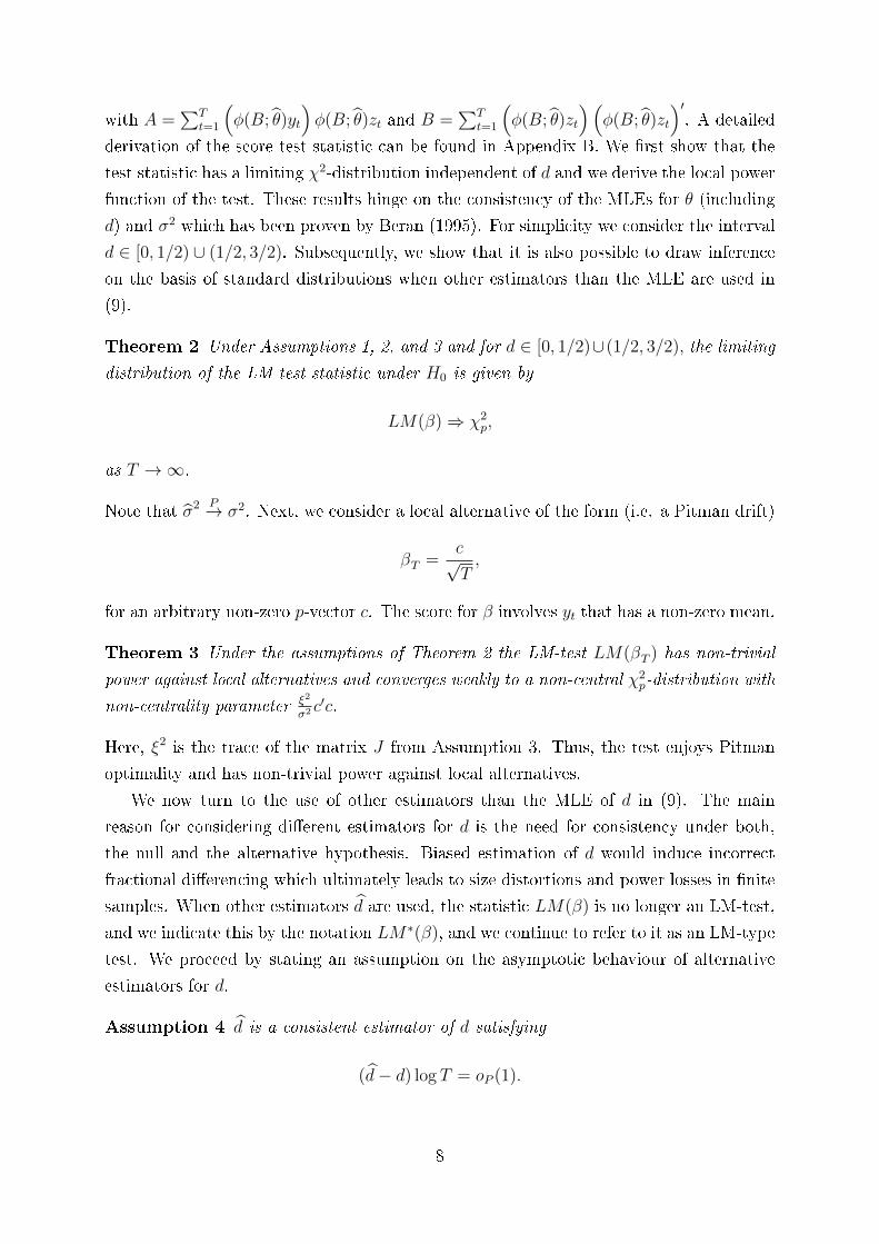
derivation of the score test statistic can be found in Appendix B. We �rst show that the
test statistic has a limiting χ2-distribution independent of d and we derive the local power
function of the test. These results hinge on the consistency of the MLEs for θ (including
d) and σ2 which has been proven by Beran (1995). For simplicity we consider the interval
d ∈ [0, 1/2) ∪ (1/2, 3/2). Subsequently, we show that it is also possible to draw inference
on the basis of standard distributions when other estimators than the MLE are used in
(9).
Theorem 2 Under Assumptions 1, 2, and 3 and for d ∈ [0, 1/2)∪(1/2, 3/2), the limiting
distribution of the LM test statistic under H0 is given by
LM(β)⇒ χ2p,
as T →∞.
Note that σ2 P→ σ2. Next, we consider a local alternative of the form (i.e. a Pitman drift)
βT =c√T,
for an arbitrary non-zero p-vector c. The score for β involves yt that has a non-zero mean.
Theorem 3 Under the assumptions of Theorem 2 the LM-test LM(βT ) has non-trivial
power against local alternatives and converges weakly to a non-central χ2p-distribution with
non-centrality parameter ξ2
σ2 c′c.
Here, ξ2 is the trace of the matrix J from Assumption 3. Thus, the test enjoys Pitman
optimality and has non-trivial power against local alternatives.
We now turn to the use of other estimators than the MLE of d in (9). The main
reason for considering di�erent estimators for d is the need for consistency under both,
the null and the alternative hypothesis. Biased estimation of d would induce incorrect
fractional di�erencing which ultimately leads to size distortions and power losses in �nite
samples. When other estimators d are used, the statistic LM(β) is no longer an LM-test,
and we indicate this by the notation LM∗(β), and we continue to refer to it as an LM-type
test. We proceed by stating an assumption on the asymptotic behaviour of alternative
estimators for d.
Assumption 4 d is a consistent estimator of d satisfying
(d− d) log T = oP (1).
8

Assumption 4 is su�ciently general to include the most commonly used consistent esti-
mators, such as the log-periodogram regression estimator of Geweke and Porter-Hudak
(1983), the Gaussian semiparametric or local Whittle estimator of Robinson (1995) as
well as the exact local Whittle estimator by Shimotsu and Phillips (2005).
Theorem 4 Under Assumptions 1, 2, 3, and 4, and for d ∈ [0, 1/2) ∪ (1/2, 3/2), the
limiting distribution of the LM∗-statistic under H0 is given by
LM∗(β)⇒ χ2p,
as T →∞.
Thus, the limiting null distribution of LM∗ coincides with that of the LM-test in Theorem
2 and is thus independent of the unknown integration order. In this sense, it is also
possible to draw valid inference on β under an unknown order of integration even when
using other estimators satisfying Assumption 4 than the MLE. The results for the local
power function, see Theorem 3, carry over to LM∗.2
3.2 Stochastic Regressors
So far, the analysis has focussed on the case of deterministic regressors. However, the
new LM∗ testing approach can be applied in situations with stochastic regressors, too.
As before we consider the model
yt = β′zt + et, (10)
where now yt and zt are type II fractional processes of order d1. The parameter vector
β = (β1, . . . , βp)′and zt are both p-dimensional. As we focus on fractional cointegration
below we assume that all components of zt are integrated of the same order d1 and that
E[z′itzjt] = 0 for i 6= j. Furthermore, we assume that d1 > 1/2 holds. The error term et is
assumed to be a type II fractional process of order I(d0) with d0 < d1 and d1−d0 > 1/2+ε
for some ε > 0. Consider testing the hypothesis
H0 : β = β0, against H1 : β 6= β0, (11)
with β and β0 being p-vectors. Imposing an other restriction than β0 = 0 does not change
our results. As we are aware that this restriction might have some attraction to keep the
notation simple it is of minor practical relevance in this set up and therefore we do not
impose it in this section. Regarding exogeneity of the regressors we impose the following
assumption:
2Although the proof of Theorem 4 is speci�c to the case of deterministic regressors, it is a generalproperty that when plug-in estimators of nuisance parameters (such as d) converge su�ciently fast, thenlimiting distributions and local power of tests are una�ected (see, e.g., Jansson and Nielsen, 2012).
9

Assumption 5 The zt are strictly exogenous with
φ(B, θ1)zt = u1t
and
φ(B, θ0)et = ut,
and u1t and ut ful�ll Assumption 1. Here, φ(B, θ) is de�ned as before with θ1 containing
d1 and θ0 containing d0 as orders of integration.
The log-likelihood function in this framework is similar to the case of non-stochastic
regressors and can be found in Appendix B where also the derivation of the test statistic
is located. By θ and σ2 we denote the ML-estimator for θ and σ2, respectively. By
evaluating the scores at β = β0, we obtain by similar arguments as in the case of non-
stochastic regressors that the LM-test statistic is given by
LM(β) =1
σ2A′B−1A (12)
with A =∑T
t=1(φ(B, θ)(yt − β′
0zt)(φ(B, θ)zt) and B =∑T
t=1(φ(B, θ)zt)(φ(B, θ)zt)′. The
test statistic (12) in the case of stochastic exogenous regressors is thus of exactly the
same form as the test statistic (9) for non-stochastic regressors. However, it should be
mentioned that the term φ(B, θ)zt is now stochastic and integrated of order d1 − d0.
Theorem 5 Under Assumptions 1, 2 and 5, the limiting distribution of the LM test
statistic under H0 is given by
LM(β)⇒ χ2p
as T →∞.
Thus, neither the fractional integration order of the regressors (d1) nor the fractional order
of the errors (d0) in�uences the distribution of the test statistic which is similar to the
case of deterministic regressors, a standard one. By similar arguments as in Theorem 4
we can use other estimators for d1 and d0 than the MLE as long as they ful�ll Assumption
4. The test has local power also in the case of stochastic exogenous regressors.
Theorem 6 Under the assumptions of Theorem 5, the LM-test LM(βT ) has non-trivial
power against local alternatives and converges to a non-central χ2p-distribution with non-
centrality parameter ξ2
σ2 c′c.
We now relax the assumption of zt being exogenous and derive the limiting distribution
of the LM-type test for this case. Our result shows that the test is biased when no
endogeneity correction is applied. As demonstrated in the Monte Carlo section, correcting
10
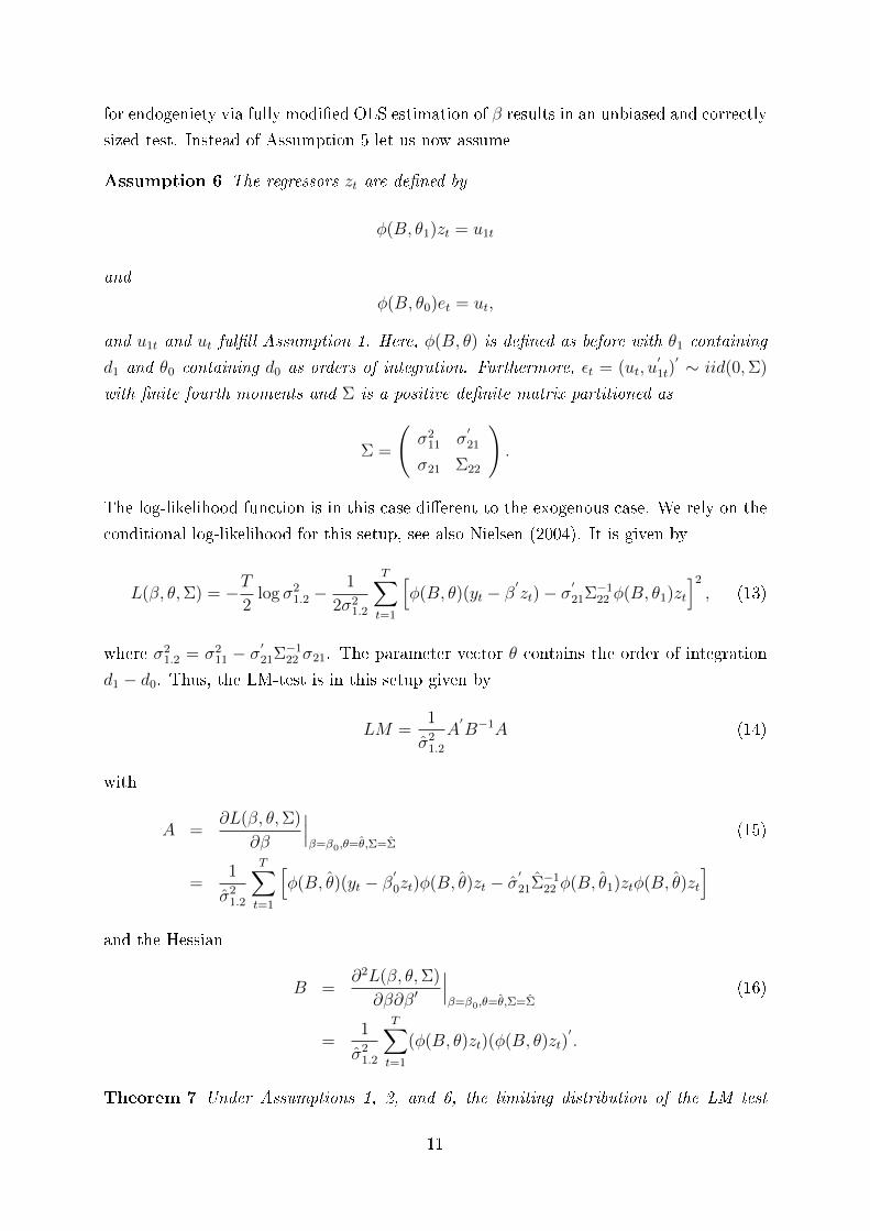
for endogeniety via fully modi�ed OLS estimation of β results in an unbiased and correctly
sized test. Instead of Assumption 5 let us now assume
Assumption 6 The regressors zt are de�ned by
φ(B, θ1)zt = u1t
and
φ(B, θ0)et = ut,
and u1t and ut ful�ll Assumption 1. Here, φ(B, θ) is de�ned as before with θ1 containing
d1 and θ0 containing d0 as orders of integration. Furthermore, εt = (ut, u′1t)′ ∼ iid(0,Σ)
with �nite fourth moments and Σ is a positive de�nite matrix partitioned as
Σ =
(σ2
11 σ′21
σ21 Σ22
).
The log-likelihood function is in this case di�erent to the exogenous case. We rely on the
conditional log-likelihood for this setup, see also Nielsen (2004). It is given by
L(β, θ,Σ) = −T2
log σ21.2 −
1
2σ21.2
T∑t=1
[φ(B, θ)(yt − β
′zt)− σ
′
21Σ−122 φ(B, θ1)zt
]2
, (13)
where σ21.2 = σ2
11 − σ′21Σ−1
22 σ21. The parameter vector θ contains the order of integration
d1 − d0. Thus, the LM-test is in this setup given by
LM =1
σ21.2
A′B−1A (14)
with
A =∂L(β, θ,Σ)
∂β
∣∣∣β=β0,θ=θ,Σ=Σ
(15)
=1
σ21.2
T∑t=1
[φ(B, θ)(yt − β
′
0zt)φ(B, θ)zt − σ′
21Σ−122 φ(B, θ1)ztφ(B, θ)zt
]and the Hessian
B =∂2L(β, θ,Σ)
∂β∂β′
∣∣∣β=β0,θ=θ,Σ=Σ
(16)
=1
σ21.2
T∑t=1
(φ(B, θ)zt)(φ(B, θ)zt)′.
Theorem 7 Under Assumptions 1, 2, and 6, the limiting distribution of the LM test
11
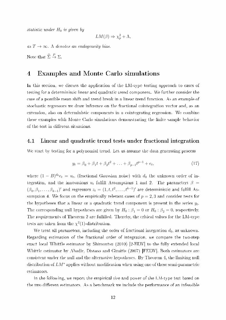
statistic under H0 is given by
LM(β)⇒ χ2p + Λ,
as T →∞. Λ denotes an endogeneity bias.
Note that ΣP→ Σ.
4 Examples and Monte Carlo simulations
In this section, we discuss the application of the LM-type testing approach to cases of
testing for a deterministic linear and quadratic trend component. We further consider the
case of a possible mean shift and trend break in a linear trend function. As an example of
stochastic regressors we draw inference on the fractional cointegration vector and, as an
extension, also on deterministic components in a cointegrating regression. We combine
these examples with Monte Carlo simulations demonstrating the �nite sample behavior
of the test in di�erent situations.
4.1 Linear and quadratic trend tests under fractional integration
We start by testing for a polynomial trend. Let us assume the data generating process
yt = β0 + β1t+ β2t2 + . . .+ βp−1t
p−1 + et, (17)
where (1 − B)d0et = ut, (fractional Gaussian noise) with d0 the unknown order of in-
tegration, and the innovations ut ful�ll Assumptions 1 and 2. The parameters β =
(β0, β1, . . . , βk−1)′ and regressors zt = (1, t, t2, . . . , tk−1)′ are deterministic and ful�ll As-
sumption 4. We focus on the empirically relevant cases of p = 2, 3 and consider tests for
the hypotheses that a linear or a quadratic trend component is present in the series yt.
The corresponding null hypotheses are given by H0 : β1 = 0 or H0 : β2 = 0, respectively.
The requirements of Theorem 2 are ful�lled. Thereby, the critical values for the LM-type
tests are taken from the χ2(1)-distribution.
We treat all parameters, including the order of fractional integration d0, as unknown.
Regarding estimation of the fractional order of integration, we compare the two-step
exact local Whittle estimator by Shimoutsu (2010) [2-ELW] to the fully extended local
Whittle estimator by Abadir, Distaso and Giraitis (2007) [FELW]. Both estimators are
consistent under the null and the alternative hypotheses. By Theorem 4, the limiting null
distribution of LM∗ applies without modi�cation when using one of these semi-parametric
estimators.
In the following, we report the empirical size and power of the LM-type test based on
the two di�erent estimators. As a benchmark we include the performance of an infeasible
12

Table 1: Empirical size and power for testing H0 : β1 = 0 or H0 : β2 = 0, T = 500,normally distributed errors
Linear Trend
d0 Stat Size avg d0 sd d0 Power avg d0 sd d0
0 2-ELW 0.057 0.001 0.057 1.000 0.000 0.057
FELW 0.069 -0.013 0.055 1.000 -0.014 0.055
Infeasible 0.050 0.000 0.000 1.000 0.000 0.000
0.4 2-ELW 0.059 0.403 0.058 0.836 0.402 0.058
FELW 0.074 0.380 0.060 0.869 0.379 0.060
Infeasible 0.048 0.400 0.000 0.872 0.400 0.000
0.8 2-ELW 0.053 0.810 0.057 0.104 0.808 0.057
FELW 0.075 0.783 0.055 0.140 0.781 0.055
Infeasible 0.050 0.800 0.000 0.102 0.800 0.000
1.2 2-ELW 0.049 1.212 0.055 0.058 1.211 0.055
FELW 0.084 1.174 0.054 0.096 1.173 0.054
Infeasible 0.047 1.200 0.000 0.052 1.200 0.000
Quadratic Trend
d0 Stat Size avg d0 sd d0 Power avg d0 sd d0
0 2-ELW 0.065 -0.010 0.059 1.000 -0.009 0.059
FELW 0.075 -0.026 0.057 1.000 -0.025 0.058
Infeasible 0.051 0.000 0.000 1.000 0.000 0.000
0.4 2-ELW 0.062 0.392 0.060 0.993 0.393 0.060
FELW 0.079 0.369 0.062 0.996 0.370 0.063
Infeasible 0.051 0.400 0.000 0.997 0.400 0.000
0.8 2-ELW 0.052 0.800 0.060 0.210 0.801 0.060
FELW 0.075 0.773 0.057 0.265 0.774 0.057
Infeasible 0.048 0.800 0.000 0.204 0.800 0.000
1.2 2-ELW 0.055 1.204 0.057 0.070 1.204 0.057
FELW 0.084 1.164 0.056 0.104 1.164 0.056
Infeasible 0.050 1.200 0.000 0.066 1.200 0.000
test using the true parameter d0 instead of an estimate. The nominal signi�cance level
equals �ve percent, the sample size is T = 500 and the number of Monte Carlo replications
equals 5,000 for each single experiment. All computations are carried out in MATLAB.3
In addition to the size and power results, we also report the Monte Carlo mean and
standard deviation of the 2ELW and the FELW estimator. The importance of normality
is investigated by considering non-normal errors. To this end, we generate fat-tailed t(6)-
distributed and skewed standardized χ2(5)-distributed errors. In these cases, estimation
of β is achieved via quasi-ML assuming normality for constructing the likelihood function.
3We would like to thank Karim Abadir, Walter Distaso and Luidas Giraitis for sharing their MATLABcode for the FELW estimator with us. The code for the Shimotsu (2010) estimator can be found on theauthor's webpage.
13
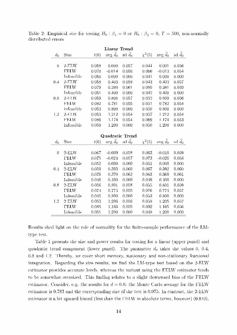
Table 2: Empirical size for testing H0 : β1 = 0 or H0 : β2 = 0, T = 500, non-normallydistributed errors
Linear Trend
d0 Stat t(6) avg d0 sd d0 χ2(5) avg d0 sd d0
0 2-ELW 0.058 0.000 0.057 0.044 0.001 0.056
FELW 0.070 -0.014 0.056 0.066 -0.013 0.054
Infeasible 0.050 0.000 0.000 0.041 0.000 0.000
0.4 2-ELW 0.058 0.403 0.058 0.043 0.403 0.057
FELW 0.079 0.380 0.061 0.080 0.381 0.059
Infeasible 0.051 0.400 0.000 0.042 0.400 0.000
0.8 2-ELW 0.059 0.808 0.057 0.052 0.809 0.056
FELW 0.082 0.781 0.055 0.051 0.782 0.054
Infeasible 0.053 0.800 0.000 0.050 0.800 0.000
1.2 2-ELW 0.053 1.212 0.054 0.057 1.212 0.054
FELW 0.086 1.174 0.054 0.069 1.174 0.053
Infeasible 0.050 1.200 0.000 0.050 1.200 0.000
Quadratic Trend
d0 Stat t(6) avg d0 sd d0 χ2(5) avg d0 sd d0
0 2-ELW 0.067 -0.009 0.058 0.063 -0.010 0.059
FELW 0.075 -0.024 0.057 0.073 -0.026 0.058
Infeasible 0.052 0.000 0.000 0.051 0.000 0.000
0.4 2-ELW 0.059 0.393 0.060 0.067 0.392 0.060
FELW 0.076 0.370 0.062 0.083 0.369 0.061
Infeasible 0.046 0.400 0.000 0.049 0.400 0.000
0.8 2-ELW 0.056 0.801 0.058 0.055 0.801 0.059
FELW 0.074 0.775 0.055 0.076 0.774 0.057
Infeasible 0.045 0.800 0.000 0.053 0.800 0.000
1.2 2-ELW 0.053 1.206 0.056 0.058 1.205 0.057
FELW 0.085 1.166 0.055 0.092 1.165 0.056
Infeasible 0.051 1.200 0.000 0.048 1.200 0.000
Results shed light on the role of normality for the �nite-sample performance of the LM-
type test.
Table 1 presents the size and power results for testing for a linear (upper panel) and
quadratic trend component (lower panel). The parameter d0 takes the values 0, 0.4,
0.8 and 1.2. Thereby, we cover short memory, stationary and non-stationary fractional
integration. Regarding the size results, we �nd the LM-type test based on the 2-ELW
estimator provides accurate levels, whereas the variant using the FELW estimator tends
to be somewhat oversized. This �nding relates to a slight downward bias of the FELW
estimator. Consider, e.g. the results for d = 0.8: the Monte Carlo average for the FELW
estimator is 0.783 and the corresponding size of the test is 0.075. In contrast, the 2-ELW
estimator is a bit upward biased (less than the FELW in absolute terms, however) (0.810),
14
but the simulated size is 0.053. Noteworthy, the FELW estimator has a smaller standard
deviation (0.055 versus 0.057). An even slight downward bias implies that the series will
not be di�erenced to I(0), but to a small positive order of integration. The LM-type
test appears to be sensitive towards such a bias and therefore, we recommend to use the
2-ELW estimator for testing linear trends. This �nding also holds for testing quadratic
trend components. The infeasible test has very accurate size in all cases. Interestingly,
the LM-type test based on the 2-ELW estimator performs very well in comparison to the
infeasible test. The results for both estimators show their merits as they perform very
well under H0 and H1.
The reported results for the empirical power (β1 = 0.005 and β2 = 0.00005) indicate
similar performances amongst the di�erent variants of the test. It shall be noted that
the values for β1 and β2 are �xed for di�erent values of d0. The larger the fractional
order of integration, the larger is the variance of the stochastic part of the process and
the more di�cult is the detection of a linear or quadratic trend component. Thus, it is
not surprising that the power decreases as d0 increases.
Table 2 presents size results for fat-tailed and skewed errors. The results are very
similar to the ones obtained for normally distributed errors. The main conclusions do
not change and the results suggest robustness against a misspeci�cation of the error
distribution. The LM-type test also performs well when errors are assumed to be normal,
but are fat-tailed or skewed instead.
4.2 Structural change tests for intercept and slope of a linear
trend model under fractional integration
We also consider the problem of testing for a break in the intercept and slope parameter
of a linear trend function. A slightly di�erent model (without intercept shift) is studied in
Iacone et al. (2013a, 2013b). They consider the behavior of �xed-b tests for trend breaks
and robustify those to the fractional case. The model of our interest, see also Perron and
Yabu (2009) for a quasi-feasible GLS approach in case of I(0) or I(1) errors, is given by
yt = β0 + δ0DUt + β1t+ δ1DTt + et (18)
where the variables DUt and DTt are given by
DUt = 1(t > c),
DTt = 1(t > c)(t− bcT c).
The relative break point is denoted by c and c ∈ [τL, τU ] =: Λ ⊂ [0, 1] and τL and τU
are the lower and upper bounds of the interval to which the break point is restricted.
15
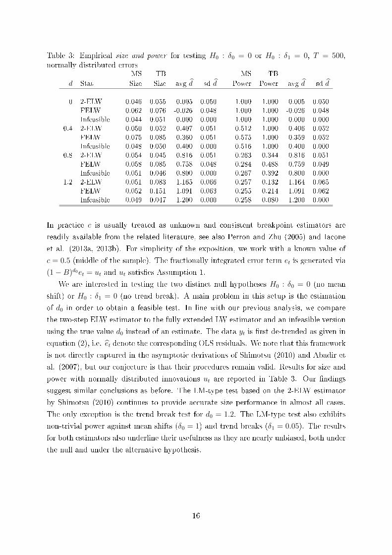
Table 3: Empirical size and power for testing H0 : δ0 = 0 or H0 : δ1 = 0, T = 500,normally distributed errors
MS TB MS TB
d Stat Size Size avg d sd d Power Power avg d sd d
0 2-ELW 0.046 0.055 0.005 0.050 1.000 1.000 0.005 0.050
FELW 0.062 0.076 -0.026 0.048 1.000 1.000 -0.026 0.048
Infeasible 0.044 0.051 0.000 0.000 1.000 1.000 0.000 0.000
0.4 2-ELW 0.050 0.052 0.407 0.051 0.512 1.000 0.406 0.052
FELW 0.075 0.085 0.360 0.051 0.575 1.000 0.359 0.052
Infeasible 0.048 0.050 0.400 0.000 0.516 1.000 0.400 0.000
0.8 2-ELW 0.054 0.045 0.816 0.051 0.263 0.344 0.816 0.051
FELW 0.058 0.085 0.758 0.048 0.284 0.488 0.759 0.049
Infeasible 0.051 0.046 0.800 0.000 0.267 0.392 0.800 0.000
1.2 2-ELW 0.051 0.083 1.165 0.066 0.257 0.132 1.164 0.065
FELW 0.052 0.151 1.091 0.063 0.255 0.214 1.091 0.062
Infeasible 0.049 0.047 1.200 0.000 0.258 0.080 1.200 0.000
In practice c is usually treated as unknown and consistent breakpoint estimators are
readily available from the related literature, see also Perron and Zhu (2005) and Iacone
et al. (2013a, 2013b). For simplicity of the exposition, we work with a known value of
c = 0.5 (middle of the sample). The fractionally integrated error term et is generated via
(1−B)d0et = ut and ut satis�es Assumption 1.
We are interested in testing the two distinct null hypotheses H0 : δ0 = 0 (no mean
shift) or H0 : δ1 = 0 (no trend break). A main problem in this setup is the estimation
of d0 in order to obtain a feasible test. In line with our previous analysis, we compare
the two-step ELW estimator to the fully extended LW estimator and an infeasible version
using the true value d0 instead of an estimate. The data yt is �rst de-trended as given in
equation (2), i.e. et denote the corresponding OLS residuals. We note that this framework
is not directly captured in the asymptotic derivations of Shimotsu (2010) and Abadir et
al. (2007), but our conjecture is that their procedures remain valid. Results for size and
power with normally distributed innovations ut are reported in Table 3. Our �ndings
suggest similar conclusions as before. The LM-type test based on the 2-ELW estimator
by Shimotsu (2010) continues to provide accurate size performance in almost all cases.
The only exception is the trend break test for d0 = 1.2. The LM-type test also exhibits
non-trivial power against mean shifts (δ0 = 1) and trend breaks (δ1 = 0.05). The results
for both estimators also underline their usefulness as they are nearly unbiased, both under
the null and under the alternative hypothesis.
16
4.3 Inference on the fractional cointegration vector and deter-
ministic trends
Cointegration is a natural example in the case of stochastic regressors. In the standard
Engle and Granger (1987) cointegration model it is assumed that the data series (yt, zt)
are I(1), and cointegration exists if one or more linear combinations of the series are I(0).
Thus, in our regression framework
yt = β′zt + et,
cointegration is implied if et ∼ I(0), and spurious regression if et ∼ I(1). As in Vogelsang's
approach to trend testing, it is critical that the order of integration of the errors (d0) is
known to be one of only two possible values (again, 0 or 1). In practical applications, other
possible values for d must often be considered, as well. In case of fractional cointegration,
zt may be (possibly fractionally) integrated of order d1, say, not necessarily restricting
d1 to unity. Fractional cointegration exists if the errors are integrated of lower order,
et ∼ I(d0), with d0 < d1. In this case, yt is integrated of order d1, too, and the series yt
and zt move together in the long run, in a more general sense not necessarily implying
standard I(1)−I(0) cointegration. In particular, d may take values in a continuum, rather
than being restricted to be either 0 or 1. In particular, we consider the simple case of
fractional cointegration
yt = βzt + et (19)
(1−B)d0et = ut (20)
(1−B)d1zt = u1t (21)
satisfying Assumption 6. yt and zt are scalar type II fractional processes of order d1 > 1/2.
The errors et are integrated of order d0 = 0 for simplicity. This type of triangular system
has been considered by Phillips (1991) for the case of standard cointegration, and by
Nielsen (2004) for fractional cointegration, and is easily extended to the case of multiple
cointegrating relations. Evidently, zt are stochastic regressors in the cointegration case,
whether standard or fractional, and the latter is a natural application of our results in
Section 3.2. Estimation of the cointegration system under unknown order of integration
has been considered by Robinson and Hualde (2003).
With yt and zt moving together in the long run, interest centers on the cointegrating
relation, as described by the cointegrating vector β. The linear hypothesis of interest is
given by H0 : β = 1 which is a restriction on the sub-cointegrating vector and imposes
a one-to-one long-run relationship between yt and zt. This is a typical example for a
hypothesis of long-run unbiasedness in predictive regressions, e.g., testing expectation
17
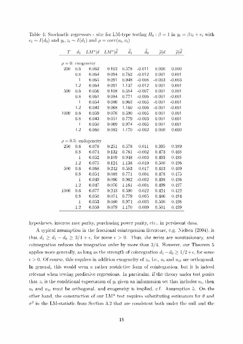
Table 4: Stochastic regressors - size for LM-type testing H0 : β = 1 in yt = βzt + et withet ∼ I(d0) and yt, zt ∼ I(d1) and ρ = corr(ut, vt)
T d1 LM∗|d LM∗|d d1 d0 ρ|d ρ|d
ρ = 0: exogeneity250 0.6 0.062 0.103 0.578 -0.011 0.000 0.000
0.8 0.064 0.094 0.762 -0.012 0.001 0.001
1 0.065 0.091 0.948 -0.008 -0.003 -0.003
1.2 0.064 0.091 1.137 -0.012 0.001 0.001
500 0.6 0.056 0.108 0.584 -0.007 0.001 0.001
0.8 0.061 0.084 0.771 -0.006 -0.001 -0.001
1 0.054 0.086 0.962 -0.005 -0.001 -0.001
1.2 0.042 0.068 1.160 -0.006 -0.001 -0.001
1000 0.6 0.059 0.076 0.590 -0.005 0.001 0.001
0.8 0.043 0.051 0.779 -0.003 0.001 0.001
1 0.050 0.069 0.974 -0.005 0.001 0.001
1.2 0.060 0.083 1.170 -0.002 0.000 0.000
ρ = 0.5: endogeneity250 0.6 0.078 0.251 0.578 0.011 0.395 0.389
0.8 0.074 0.132 0.761 -0.002 0.473 0.468
1 0.052 0.109 0.948 -0.003 0.493 0.488
1.2 0.075 0.124 1.138 -0.010 0.500 0.496
500 0.6 0.068 0.242 0.583 0.017 0.413 0.409
0.8 0.054 0.088 0.771 0.004 0.478 0.475
1 0.049 0.096 0.962 -0.002 0.498 0.496
1.2 0.047 0.076 1.161 -0.004 0.499 0.497
1000 0.6 0.077 0.243 0.590 0.022 0.424 0.422
0.8 0.050 0.074 0.779 0.005 0.486 0.484
1 0.053 0.080 0.974 -0.003 0.500 0.498
1.2 0.059 0.079 1.170 0.000 0.501 0.499
hypotheses, interest rate parity, purchasing power parity, etc., in persistent data.
A typical assumption in the fractional cointegration literature, e.g. Nielsen (2004), is
that d1 ≥ d1 − d0 ≥ 3/4 + ε, for some ε > 0. Thus, the series are nonstationary, and
cointegration reduces the integration order by more than 3/4. However, our Theorem 5
applies more generally, as long as the strength of cointegration d1−d0 ≥ 1/2+ ε, for some
ε > 0. Of course, this requires in addition exogeneity of zt, i.e., ut and u1t are orthogonal.
In general, this would seem a rather restrictive form of cointegration, but it is indeed
relevant when testing predictive regressions. In particular, if the theory under test posits
that zt is the conditional expectation of yt given an information set that includes ut, then
ut and u1t must be orthogonal, and exogeneity is implied, c.f. Assumption 5. On the
other hand, the construction of our LM* test requires substituting estimators for θ and
σ2 in the LM-statistic from Section 3.2 that are consistent both under the null and the
18
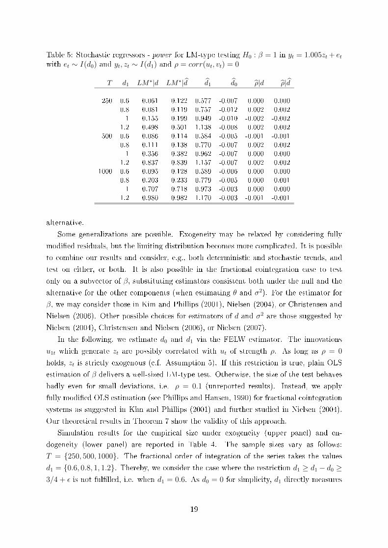
Table 5: Stochastic regressors - power for LM-type testing H0 : β = 1 in yt = 1.005zt + etwith et ∼ I(d0) and yt, zt ∼ I(d1) and ρ = corr(ut, vt) = 0
T d1 LM∗|d LM∗|d d1 d0 ρ|d ρ|d
250 0.6 0.061 0.122 0.577 -0.007 0.000 0.000
0.8 0.081 0.119 0.757 -0.012 0.002 0.002
1 0.155 0.199 0.949 -0.010 -0.002 -0.002
1.2 0.498 0.501 1.138 -0.008 0.002 0.002
500 0.6 0.086 0.114 0.584 -0.005 -0.001 -0.001
0.8 0.111 0.138 0.770 -0.007 0.002 0.002
1 0.356 0.382 0.962 -0.007 0.000 0.000
1.2 0.837 0.839 1.157 -0.007 0.002 0.002
1000 0.6 0.095 0.128 0.589 -0.006 0.000 0.000
0.8 0.203 0.233 0.779 -0.005 0.000 0.001
1 0.707 0.718 0.973 -0.003 0.000 0.000
1.2 0.980 0.982 1.170 -0.003 -0.001 -0.001
alternative.
Some generalizations are possible. Exogeneity may be relaxed by considering fully
modi�ed residuals, but the limiting distribution becomes more complicated. It is possible
to combine our results and consider, e.g., both deterministic and stochastic trends, and
test on either, or both. It is also possible in the fractional cointegration case to test
only on a subvector of β, substituting estimators consistent both under the null and the
alternative for the other components (when estimating θ and σ2). For the estimator for
β, we may consider those in Kim and Phillips (2001), Nielsen (2004), or Christensen and
Nielsen (2006). Other possible choices for estimators of d and σ2 are those suggested by
Nielsen (2004), Christensen and Nielsen (2006), or Nielsen (2007).
In the following, we estimate d0 and d1 via the FELW estimator. The innovations
u1t which generate zt are possibly correlated with ut of strength ρ. As long as ρ = 0
holds, zt is strictly exogenous (c.f. Assumption 5). If this restriction is true, plain OLS
estimation of β delivers a well-sized LM-type test. Otherwise, the size of the test behaves
badly even for small deviations, i.e. ρ = 0.1 (unreported results). Instead, we apply
fully modi�ed OLS estimation (see Phillips and Hansen, 1990) for fractional cointegration
systems as suggested in Kim and Phillips (2001) and further studied in Nielsen (2004).
Our theoretical results in Theorem 7 show the validity of this approach.
Simulation results for the empirical size under exogeneity (upper panel) and en-
dogeneity (lower panel) are reported in Table 4. The sample sizes vary as follows:
T = {250, 500, 1000}. The fractional order of integration of the series takes the values
d1 = {0.6, 0.8, 1, 1.2}. Thereby, we consider the case where the restriction d1 ≥ d1 − d0 ≥3/4 + ε is not ful�lled, i.e. when d1 = 0.6. As d0 = 0 for simplicity, d1 directly measures
19
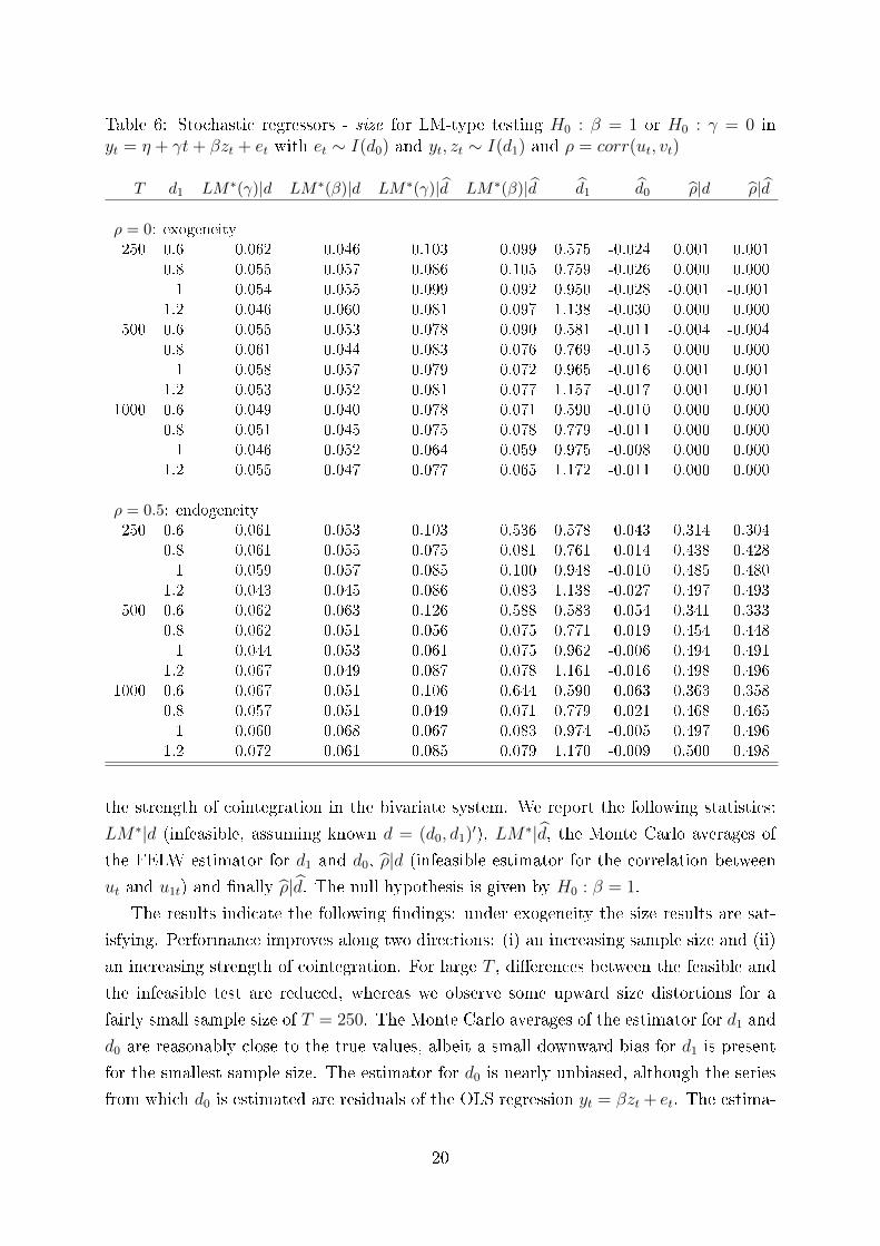
Table 6: Stochastic regressors - size for LM-type testing H0 : β = 1 or H0 : γ = 0 inyt = η + γt+ βzt + et with et ∼ I(d0) and yt, zt ∼ I(d1) and ρ = corr(ut, vt)
T d1 LM∗(γ)|d LM∗(β)|d LM∗(γ)|d LM∗(β)|d d1 d0 ρ|d ρ|d
ρ = 0: exogeneity250 0.6 0.062 0.046 0.103 0.099 0.575 -0.024 0.001 0.001
0.8 0.055 0.057 0.086 0.105 0.759 -0.026 0.000 0.000
1 0.054 0.055 0.099 0.092 0.950 -0.028 -0.001 -0.001
1.2 0.046 0.060 0.081 0.097 1.138 -0.030 0.000 0.000
500 0.6 0.055 0.053 0.078 0.090 0.581 -0.011 -0.004 -0.004
0.8 0.061 0.044 0.083 0.076 0.769 -0.015 0.000 0.000
1 0.058 0.057 0.079 0.072 0.965 -0.016 0.001 0.001
1.2 0.053 0.052 0.081 0.077 1.157 -0.017 0.001 0.001
1000 0.6 0.049 0.040 0.078 0.071 0.590 -0.010 0.000 0.000
0.8 0.051 0.045 0.075 0.078 0.779 -0.011 0.000 0.000
1 0.046 0.052 0.064 0.059 0.975 -0.008 0.000 0.000
1.2 0.055 0.047 0.077 0.065 1.172 -0.011 0.000 0.000
ρ = 0.5: endogeneity250 0.6 0.061 0.053 0.103 0.536 0.578 0.043 0.314 0.304
0.8 0.061 0.055 0.075 0.081 0.761 0.014 0.438 0.428
1 0.059 0.057 0.085 0.100 0.948 -0.010 0.485 0.480
1.2 0.043 0.045 0.086 0.083 1.138 -0.027 0.497 0.493
500 0.6 0.062 0.063 0.126 0.588 0.583 0.054 0.341 0.333
0.8 0.062 0.051 0.056 0.075 0.771 0.019 0.454 0.448
1 0.044 0.053 0.061 0.075 0.962 -0.006 0.494 0.491
1.2 0.067 0.049 0.087 0.078 1.161 -0.016 0.498 0.496
1000 0.6 0.067 0.051 0.106 0.644 0.590 0.063 0.363 0.358
0.8 0.057 0.051 0.049 0.071 0.779 0.021 0.468 0.465
1 0.060 0.068 0.067 0.083 0.974 -0.005 0.497 0.496
1.2 0.072 0.061 0.085 0.079 1.170 -0.009 0.500 0.498
the strength of cointegration in the bivariate system. We report the following statistics:
LM∗|d (infeasible, assuming known d = (d0, d1)′), LM∗|d, the Monte Carlo averages of
the FELW estimator for d1 and d0, ρ|d (infeasible estimator for the correlation between
ut and u1t) and �nally ρ|d. The null hypothesis is given by H0 : β = 1.
The results indicate the following �ndings: under exogeneity the size results are sat-
isfying. Performance improves along two directions: (i) an increasing sample size and (ii)
an increasing strength of cointegration. For large T , di�erences between the feasible and
the infeasible test are reduced, whereas we observe some upward size distortions for a
fairly small sample size of T = 250. The Monte Carlo averages of the estimator for d1 and
d0 are reasonably close to the true values, albeit a small downward-bias for d1 is present
for the smallest sample size. The estimator for d0 is nearly unbiased, although the series
from which d0 is estimated are residuals of the OLS regression yt = βzt + et. The estima-
20
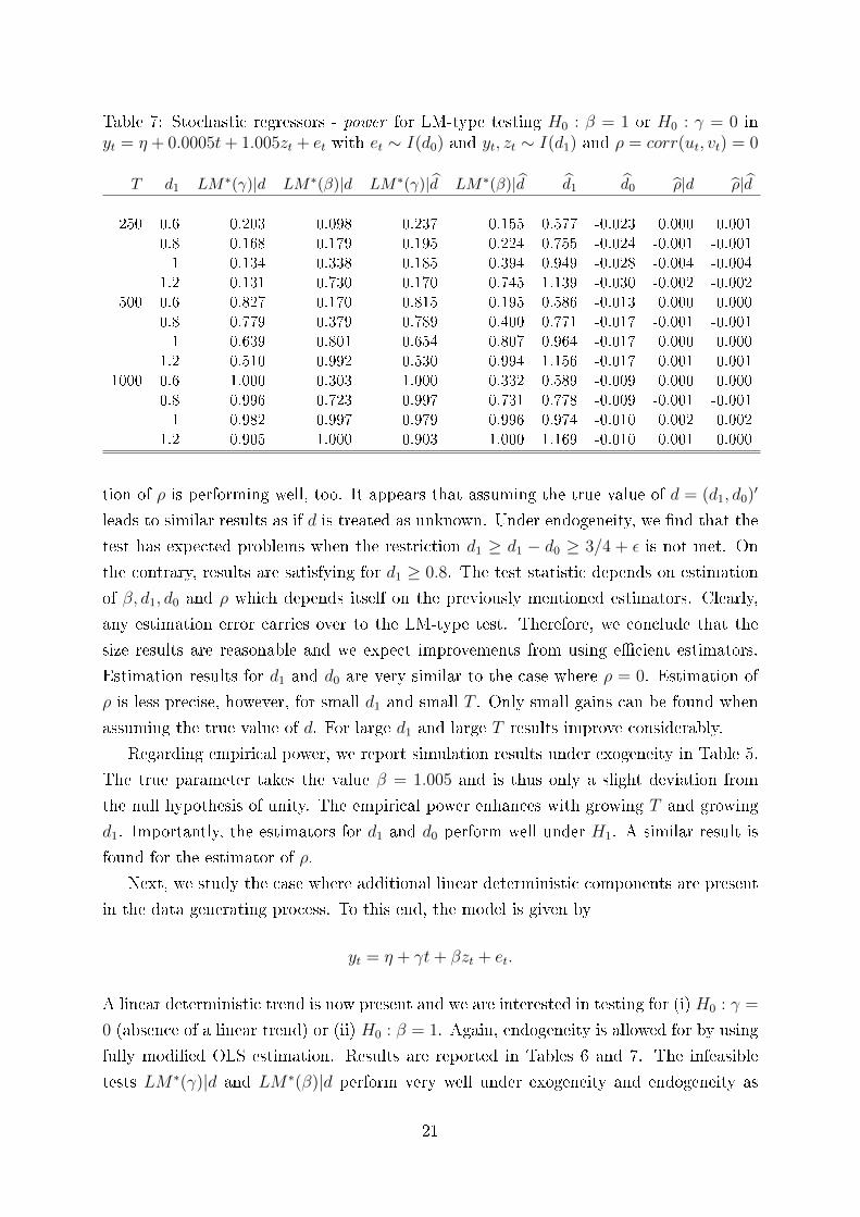
Table 7: Stochastic regressors - power for LM-type testing H0 : β = 1 or H0 : γ = 0 inyt = η + 0.0005t+ 1.005zt + et with et ∼ I(d0) and yt, zt ∼ I(d1) and ρ = corr(ut, vt) = 0
T d1 LM∗(γ)|d LM∗(β)|d LM∗(γ)|d LM∗(β)|d d1 d0 ρ|d ρ|d
250 0.6 0.203 0.098 0.237 0.155 0.577 -0.023 0.000 0.001
0.8 0.168 0.179 0.195 0.224 0.755 -0.024 -0.001 -0.001
1 0.134 0.338 0.185 0.394 0.949 -0.028 -0.004 -0.004
1.2 0.131 0.730 0.170 0.745 1.139 -0.030 -0.002 -0.002
500 0.6 0.827 0.170 0.815 0.195 0.586 -0.013 0.000 0.000
0.8 0.779 0.379 0.789 0.400 0.771 -0.017 -0.001 -0.001
1 0.639 0.801 0.654 0.807 0.964 -0.017 0.000 0.000
1.2 0.510 0.992 0.530 0.994 1.156 -0.017 0.001 0.001
1000 0.6 1.000 0.303 1.000 0.332 0.589 -0.009 0.000 0.000
0.8 0.996 0.723 0.997 0.731 0.778 -0.009 -0.001 -0.001
1 0.982 0.997 0.979 0.996 0.974 -0.010 0.002 0.002
1.2 0.905 1.000 0.903 1.000 1.169 -0.010 0.001 0.000
tion of ρ is performing well, too. It appears that assuming the true value of d = (d1, d0)′
leads to similar results as if d is treated as unknown. Under endogeneity, we �nd that the
test has expected problems when the restriction d1 ≥ d1 − d0 ≥ 3/4 + ε is not met. On
the contrary, results are satisfying for d1 ≥ 0.8. The test statistic depends on estimation
of β, d1, d0 and ρ which depends itself on the previously mentioned estimators. Clearly,
any estimation error carries over to the LM-type test. Therefore, we conclude that the
size results are reasonable and we expect improvements from using e�cient estimators.
Estimation results for d1 and d0 are very similar to the case where ρ = 0. Estimation of
ρ is less precise, however, for small d1 and small T . Only small gains can be found when
assuming the true value of d. For large d1 and large T results improve considerably.
Regarding empirical power, we report simulation results under exogeneity in Table 5.
The true parameter takes the value β = 1.005 and is thus only a slight deviation from
the null hypothesis of unity. The empirical power enhances with growing T and growing
d1. Importantly, the estimators for d1 and d0 perform well under H1. A similar result is
found for the estimator of ρ.
Next, we study the case where additional linear deterministic components are present
in the data generating process. To this end, the model is given by
yt = η + γt+ βzt + et.
A linear deterministic trend is now present and we are interested in testing for (i) H0 : γ =
0 (absence of a linear trend) or (ii) H0 : β = 1. Again, endogeneity is allowed for by using
fully modi�ed OLS estimation. Results are reported in Tables 6 and 7. The infeasible
tests LM∗(γ)|d and LM∗(β)|d perform very well under exogeneity and endogeneity as
21
well. For the feasible versions of both tests we observe some mild upward size distortions.
These can be connected to the slight downward-bias of the estimators for d1 mainly and
partly for d0. As before, the case of d1 = 0.6 leads to expected problems: The test for
H0 : β = 1 is heavily a�ected due to endogeneity and the estimator for d0 is clearly
upward biased which in turn renders the estimator for ρ to be largely downward-biased.
Unsurprisingly, even for a large sample size of T = 1000 the problem persists. On the
other hand, the test for absence of a linear trend in the cointegrating regression is nearly
una�ected as the linear trend is deterministic. While point estimation of ρ is very exact
under exogeneity, some bias arises when d1 = 0.6. As long as d ≥ 0.8, estimation of ρ
works reasonably well.
5 Conclusion
In this paper we consider testing in a general linear regression framework when the order
of possible fractional integration of the error term is unknown. We show that the ap-
proach suggested by Vogelsang (1998a) for the I(0)/I(1) case cannot be carried over to
the fractional case. Therefore, we suggest an LM-type test which is independent of the
order of fractional integration of the error term and allows testing in a general setup. The
test statistic exhibits a standard limiting distribution and has non-trivial power against
local alternatives. As possible examples covered by our approach we consider testing for
polynomial trends, mean shifts and trend breaks. Regarding stochastic regressors, we test
restrictions on the fractional cointegrating vector as well as the deterministic components
in cointegrating regressions. The LM-type test shows in all considered situations reason-
able size and power properties and thus provides a �exible technique for practitioners who
are uncertain about the possibly fractional order(s) of integration.
Appendix A
This appendix contains the proofs of our theorems, and some necessary technical lemmas
with proofs.
Proof of Theorem 1: Let us assume that yt follows the data generating process (1)
yt = β′zt + et. (22)
Under the null hypothesis H0 : β = 0 this deduces to
yt = et (23)
where we now assume that et = γet−1 + εt and εt ∼ I(δ) with δ ∈ (−1/2, 1/2). Further-
22
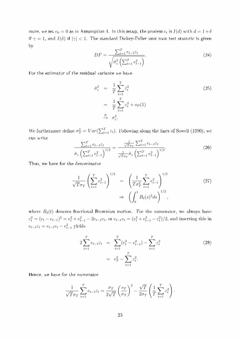
more, we set e0 = 0 as in Assumption 1. In this setup, the process et is I(d) with d = 1+δ
if γ = 1, and I(δ) if |γ| < 1. The standard Dickey-Fuller unit root test statistic is given
by
DF =
∑Tt=1 et−1εt√
σ2ε
(∑Tt=1 e
2t−1
) . (24)
For the estimator of the residual variance we have
σ2ε =
1
T
T∑t=1
ε2t (25)
=1
T
T∑t=1
ε2t + oP (1)
P→ σ2ε.
We furthermore de�ne σ2T = V ar(
∑Tt=1 εt). Following along the lines of Sowell (1990), we
can write ∑Tt=1 et−1εt
σε
(∑Tt=1 e
2t−1
)1/2=
1√TσT
∑Tt=1 et−1εt
1√TσT
σε
(∑Tt=1 e
2t−1
)1/2. (26)
Thus, we have for the denominator
1√TσT
(T∑t=1
e2t−1
)1/2
=
(1
Tσ2T
T∑t=1
e2t−1
)1/2
(27)
⇒(ˆ 1
0
Bδ(s)2ds
)1/2
,
where Bδ(t) denotes fractional Brownian motion. For the numerator, we always have
ε2t = (et− et−1)2 = e2
t + e2t−1− 2et−1et, or et−1et = (e2
t + e2t−1− ε2
t )/2, and inserting this in
et−1εt = et−1et − e2t−1 yields
2T∑t=1
et−1εt =T∑t=1
(e2t − e2
t−1)−T∑t=1
ε2t (28)
= e2T −
T∑t=1
ε2t .
Hence, we have for the numerator
1√TσT
T∑t=1
et−1εt =σT
2√T
(eTσT
)2
−√T
2σT
(1
T
T∑t=1
ε2t
).
23
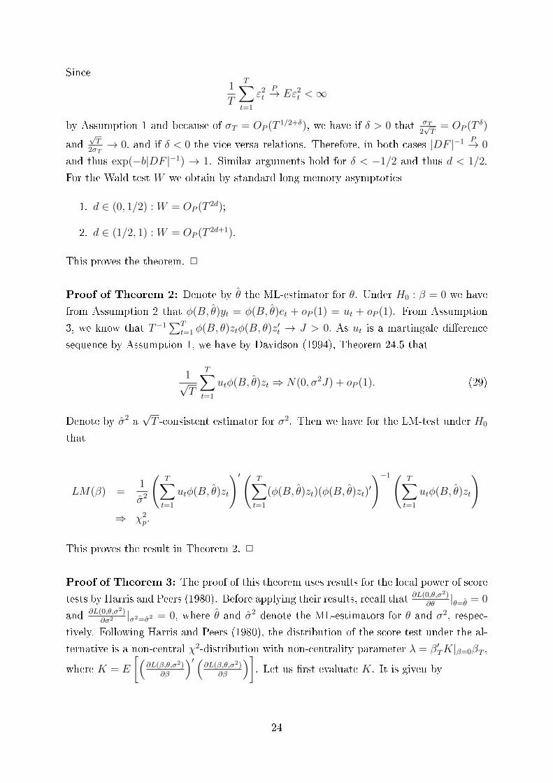
Since1
T
T∑t=1
ε2tP→ Eε2
t <∞
by Assumption 1 and because of σT = OP (T 1/2+δ), we have if δ > 0 that σT
2√T
= OP (T δ)
and√T
2σT→ 0, and if δ < 0 the vice versa relations. Therefore, in both cases |DF |−1 P→ 0
and thus exp(−b|DF |−1) → 1. Similar arguments hold for δ < −1/2 and thus d < 1/2.
For the Wald test W we obtain by standard long memory asymptotics
1. d ∈ (0, 1/2) : W = OP (T 2d);
2. d ∈ (1/2, 1) : W = OP (T 2d+1).
This proves the theorem. 2
Proof of Theorem 2: Denote by θ the ML-estimator for θ. Under H0 : β = 0 we have
from Assumption 2 that φ(B, θ)yt = φ(B, θ)et + oP (1) = ut + oP (1). From Assumption
3, we know that T−1∑T
t=1 φ(B, θ)ztφ(B, θ)z′t → J > 0. As ut is a martingale di�erence
sequence by Assumption 1, we have by Davidson (1994), Theorem 24.5 that
1√T
T∑t=1
utφ(B, θ)zt ⇒ N(0, σ2J) + oP (1). (29)
Denote by σ2 a√T -consistent estimator for σ2. Then we have for the LM-test under H0
that
LM(β) =1
σ2
(T∑t=1
utφ(B, θ)zt
)′( T∑t=1
(φ(B, θ)zt)(φ(B, θ)zt)′
)−1( T∑t=1
utφ(B, θ)zt
)⇒ χ2
p.
This proves the result in Theorem 2. 2
Proof of Theorem 3: The proof of this theorem uses results for the local power of score
tests by Harris and Peers (1980). Before applying their results, recall that ∂L(0,θ,σ2)∂θ
|θ=θ = 0
and ∂L(0,θ,σ2)∂σ2 |σ2=σ2 = 0, where θ and σ2 denote the ML-estimators for θ and σ2, respec-
tively. Following Harris and Peers (1980), the distribution of the score test under the al-
ternative is a non-central χ2-distribution with non-centrality parameter λ = β′TK|β=0βT ,
where K = E
[(∂L(β,θ,σ2)
∂β
)′ (∂L(β,θ,σ2)
∂β
)]. Let us �rst evaluate K. It is given by
24

K =1
σ4E
[T∑t=1
φ(B, θ)(yt − β′zt)(φ(B, θ)zt)′(φ(B, θ)zt)φ(B, θ)(yt − β′zt)
+T∑
s,t=1;s 6=t
φ(B, θ)(yt − β′zt)(φ(B, θ)zt)
′(φ(B, θ)zs)φ(B, θ)(ys − β′zs)
]β=0=
1
σ4
T∑t=1
E[
(φ(B, θ)yt)2 (φ(B, θ)zt)
′(φ(B, θ)zt)]
+T∑
s,t=1;s 6=t
E[φ(B, θ)ytφ(B, θ)ys(φ(B, θ)zt)
′(φ(B, θ)zs)]
=1
σ4
T∑t=1
E[u2t (φ(B, θ)zt)
′(φ(B, θ)zt)]
+T∑
s,t=1;s 6=t
E[utus(φ(B, θ)zt)
′(φ(B, θ)zs)]
=1
σ2
T∑t=1
(φ(B, θ)zt)′(φ(B, θ)zt).
From Assumption 3, we have that
T−1
T∑t=1
(φ(B, θ)zt)′(φ(B, θ)zt) = tr(T−1
T∑t=1
(φ(B, θ)zt)(φ(B, θ)zt)′)→ ξ2.
Altogether, we have
λ = β′TK|β=0βT
=1
σ2c′
1
T
T∑t=1
(φ(B, θ)zt)′(φ(B, θ)zt)c
→ ξ2
σ2c′c,
which proves the theorem. 2
Before proving Theorem 4, we de�ne a class of admissible �lters or possible lag functions
φ(z, θ), similar to the class H in Robinson (1994). In the strict sense of our approach,
this is not really necessary, as we only deal with short-term autocorrelations and possible
heteroscedasticity in the error term. However, it basically shows how wide the range of
possible �lters φ(z, θ) can be chosen, allowing for instance also for seasonality.
25
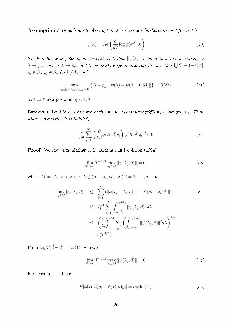
Assumption 7 In addition to Assumption 2, we assume furthermore that for real λ
ψ(λ) = Re
(d
dθlog φ(eiλ, 0)
)(30)
has �nitely many poles ρl on (−π, π] such that ‖ψ(λ)‖ is monotonically increasing as
λ → ρl− and as λ → ρl+ and there exists disjoint intervals Sl such that⋃Sl ∈ (−π, π],
ρl ∈ Sl, ρl /∈ Sk for l 6= k, and
supλ∈Sk−(ρk−δ,ρk+δ)
{|λ− ρk| ‖ψ(λ)− ψ(λ± 0.5δ)‖} = O(δη), (31)
as δ → 0 and for some η > 1/2.
Lemma 1 Let d be an estimator of the memory parameter ful�lling Assumption 4. Then,
when Assumption 7 is ful�lled,
1
σ2
T∑t=1
(∂
∂dφ(B, d)yt
)φ(B, d)yt
P→ 0. (32)
Proof: We show �rst similar as in Lemma 1 in Robinson (1994)
limT→∞
T−1/2 maxλj∈M
‖ψ(λj, d)‖ = 0, (33)
where M = {λ : π < λ < π, λ /∈ (ρl − λl, ρl + λl), l = 1, . . . , s}. It is
maxλj∈M
‖ψ(λj, d)‖ ≤r∑l=1
(‖ψ(ρl − λl, d)‖+ ‖ψ(ρl + λl, d)‖) (34)
≤ λ−1l
r∑l=1
ˆ ρl+λl
ρl−λl‖ψ(λj, d)‖dλ
≤(
2
λl
)1/2 r∑l=1
(ˆ ρl+λl
ρl−λl‖ψ(λj, d)‖2dλ
)1/2
= o(T 1/2).
From log T (d− d) = oP (1) we have
limT→∞
T−1/2 maxλj∈M
‖ψ(λj, d)‖ = 0. (35)
Furthermore, we have
E[φ(B, d)yt − φ(B, d)yt] = oP (log T ). (36)
26
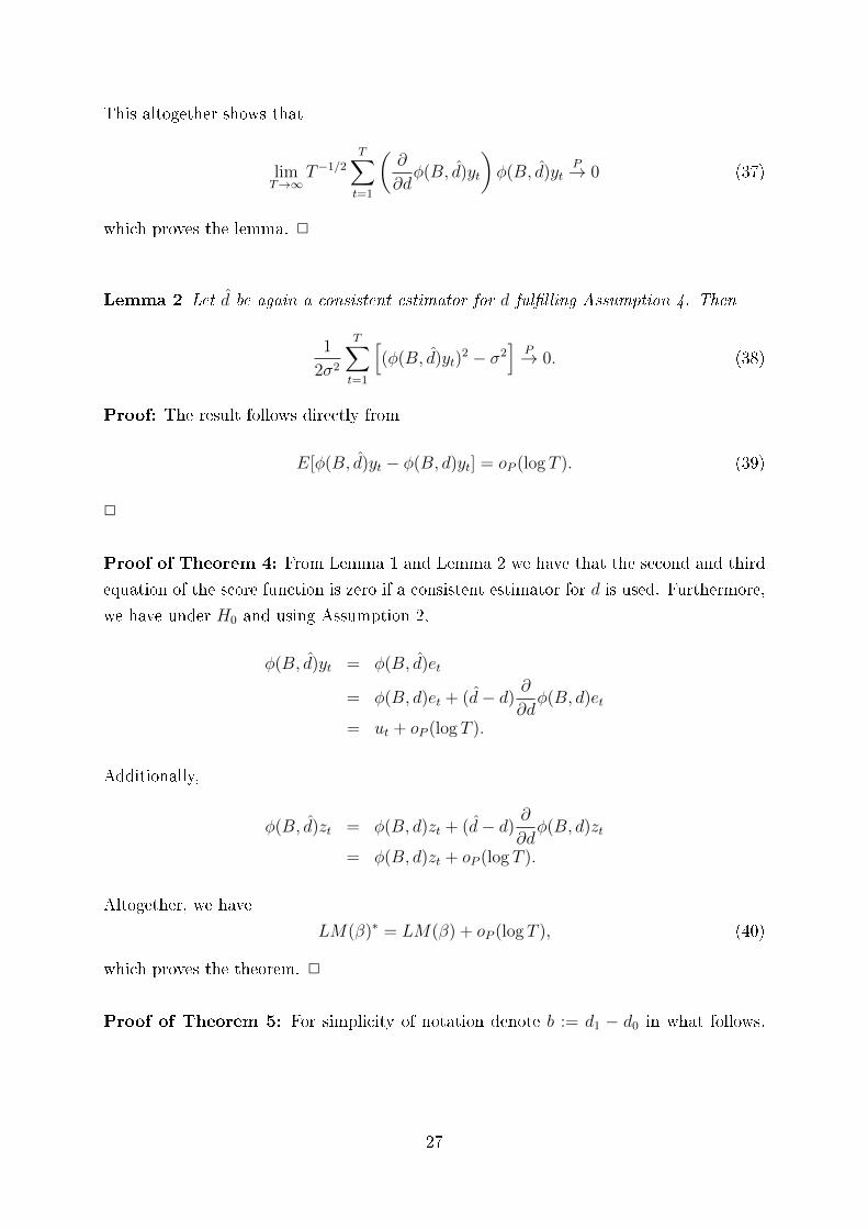
This altogether shows that
limT→∞
T−1/2
T∑t=1
(∂
∂dφ(B, d)yt
)φ(B, d)yt
P→ 0 (37)
which proves the lemma. 2
Lemma 2 Let d be again a consistent estimator for d ful�lling Assumption 4. Then
1
2σ2
T∑t=1
[(φ(B, d)yt)
2 − σ2]
P→ 0. (38)
Proof: The result follows directly from
E[φ(B, d)yt − φ(B, d)yt] = oP (log T ). (39)
2
Proof of Theorem 4: From Lemma 1 and Lemma 2 we have that the second and third
equation of the score function is zero if a consistent estimator for d is used. Furthermore,
we have under H0 and using Assumption 2,
φ(B, d)yt = φ(B, d)et
= φ(B, d)et + (d− d)∂
∂dφ(B, d)et
= ut + oP (log T ).
Additionally,
φ(B, d)zt = φ(B, d)zt + (d− d)∂
∂dφ(B, d)zt
= φ(B, d)zt + oP (log T ).
Altogether, we have
LM(β)∗ = LM(β) + oP (log T ), (40)
which proves the theorem. 2
Proof of Theorem 5: For simplicity of notation denote b := d1 − d0 in what follows.
27
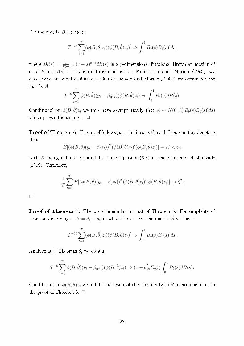
For the matrix B we have:
T−2b
T∑t=1
(φ(B, θ)zt)(φ(B, θ)zt)′ ⇒ˆ 1
0
Bb(s)Bb(s)′ds,
where Bb(r) = 1Γ(b)
´ r0
(r − s)b−1dB(s) is a p-dimensional fractional Brownian motion of
order b and B(s) is a standard Brownian motion. From Dolado and Marmol (1999) (see
also Davidson and Hashimzade, 2009 or Dolado and Marmol, 2004) we obtain for the
matrix A
T−bT∑t=1
φ(B, θ)(yt − β0zt)(φ(B, θ)zt)⇒ˆ 1
0
Bb(s)dB(s).
Conditional on φ(B, θ)zt we thus have asymptotically that A ∼ N(0,´ 1
0Bb(s)Bb(s)
′ds)
which proves the theorem. 2
Proof of Theorem 6: The proof follows just the lines as that of Theorem 3 by denoting
that
E[(φ(B, θ)(yt − β0zt))2 (φ(B, θ)zt)
′(φ(B, θ)zt)] = K <∞
with K being a �nite constant by using equation (3.8) in Davidson and Hashimzade
(2009). Therefore,
1
T
T∑t=1
E[(φ(B, θ)(yt − β0zt))2 (φ(B, θ)zt)
′(φ(B, θ)zt)]→ ξ2.
2
Proof of Theorem 7: The proof is similar to that of Theorem 5. For simplicity of
notation denote again b := d1 − d0 in what follows. For the matrix B we have:
T−2b
T∑t=1
(φ(B, θ)zt)(φ(B, θ)zt)′ ⇒ˆ 1
0
Bb(s)Bb(s)′ds,
Analogous to Theorem 5, we obtain
T−bT∑t=1
φ(B, θ)(yt − β0zt)(φ(B, θ)zt)⇒ (1− σ′21Σ−122 )
ˆ 1
0
Bb(s)dB(s).
Conditional on φ(B, θ)zt we obtain the result of the theorem by similar arguments as in
the proof of Theorem 5. 2
28
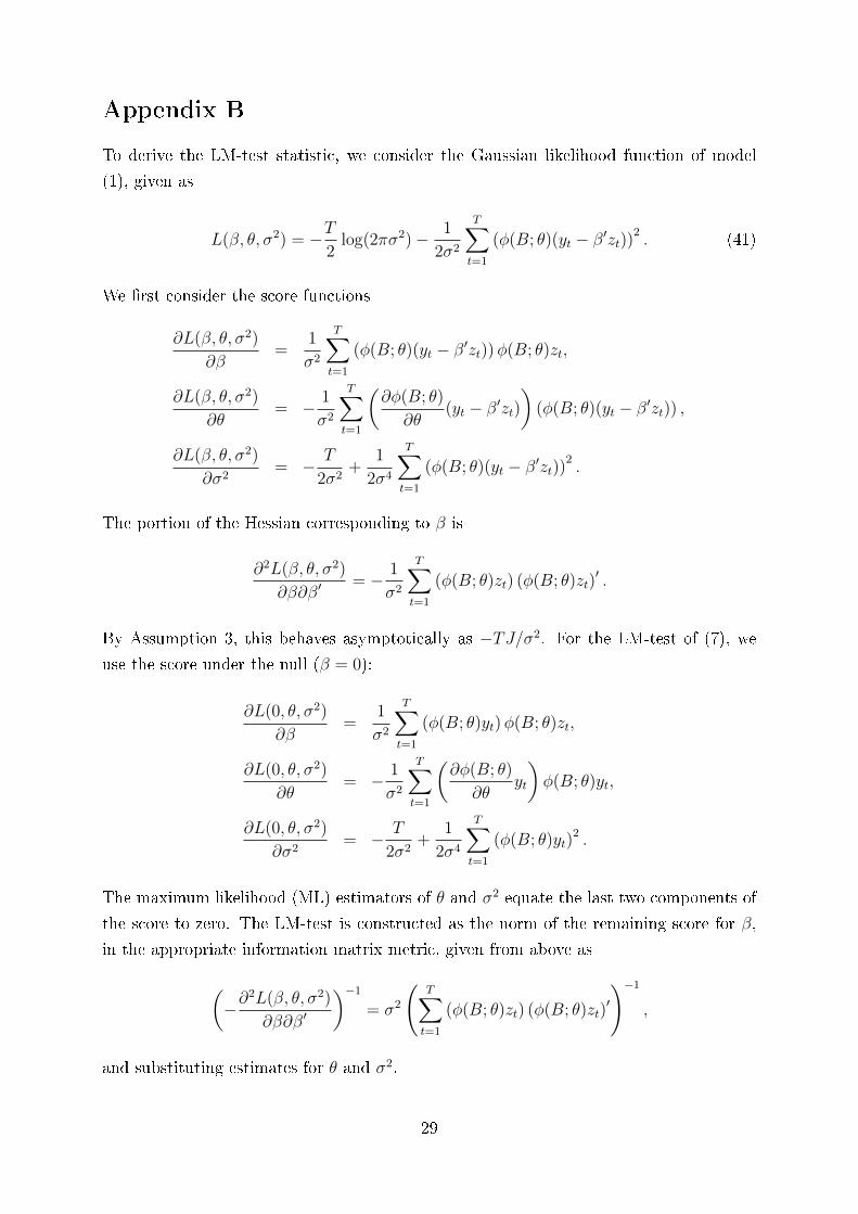
Appendix B
To derive the LM-test statistic, we consider the Gaussian likelihood function of model
(1), given as
L(β, θ, σ2) = −T2
log(2πσ2)− 1
2σ2
T∑t=1
(φ(B; θ)(yt − β′zt))2. (41)
We �rst consider the score functions
∂L(β, θ, σ2)
∂β=
1
σ2
T∑t=1
(φ(B; θ)(yt − β′zt))φ(B; θ)zt,
∂L(β, θ, σ2)
∂θ= − 1
σ2
T∑t=1
(∂φ(B; θ)
∂θ(yt − β′zt)
)(φ(B; θ)(yt − β′zt)) ,
∂L(β, θ, σ2)
∂σ2= − T
2σ2+
1
2σ4
T∑t=1
(φ(B; θ)(yt − β′zt))2.
The portion of the Hessian corresponding to β is
∂2L(β, θ, σ2)
∂β∂β′= − 1
σ2
T∑t=1
(φ(B; θ)zt) (φ(B; θ)zt)′ .
By Assumption 3, this behaves asymptotically as −TJ/σ2. For the LM-test of (7), we
use the score under the null (β = 0):
∂L(0, θ, σ2)
∂β=
1
σ2
T∑t=1
(φ(B; θ)yt)φ(B; θ)zt,
∂L(0, θ, σ2)
∂θ= − 1
σ2
T∑t=1
(∂φ(B; θ)
∂θyt
)φ(B; θ)yt,
∂L(0, θ, σ2)
∂σ2= − T
2σ2+
1
2σ4
T∑t=1
(φ(B; θ)yt)2 .
The maximum likelihood (ML) estimators of θ and σ2 equate the last two components of
the score to zero. The LM-test is constructed as the norm of the remaining score for β,
in the appropriate information matrix metric, given from above as
(−∂
2L(β, θ, σ2)
∂β∂β′
)−1
= σ2
(T∑t=1
(φ(B; θ)zt) (φ(B; θ)zt)′
)−1
,
and substituting estimates for θ and σ2.
29
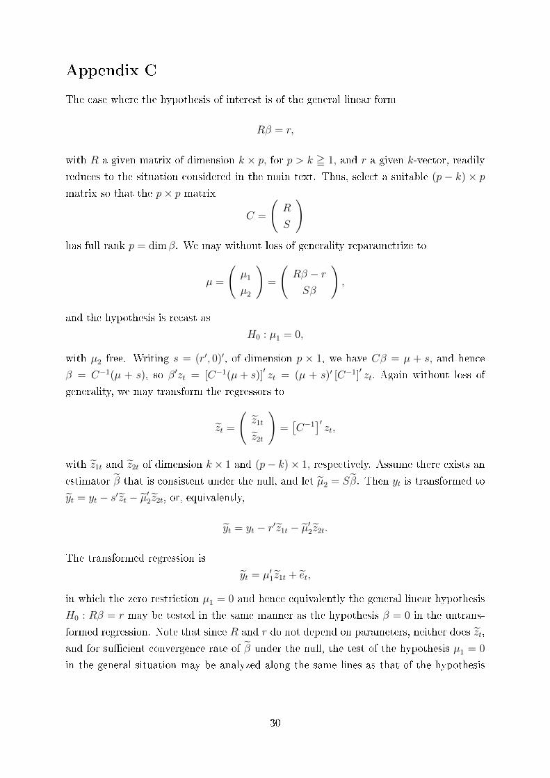
Appendix C
The case where the hypothesis of interest is of the general linear form
Rβ = r,
with R a given matrix of dimension k × p, for p > k = 1, and r a given k-vector, readily
reduces to the situation considered in the main text. Thus, select a suitable (p − k) × pmatrix so that the p× p matrix
C =
(R
S
)has full rank p = dim β. We may without loss of generality reparametrize to
µ =
(µ1
µ2
)=
(Rβ − rSβ
),
and the hypothesis is recast as
H0 : µ1 = 0,
with µ2 free. Writing s = (r′, 0)′, of dimension p × 1, we have Cβ = µ + s, and hence
β = C−1(µ + s), so β′zt = [C−1(µ+ s)]′zt = (µ + s)′ [C−1]
′zt. Again without loss of
generality, we may transform the regressors to
zt =
(z1t
z2t
)=[C−1
]′zt,
with z1t and z2t of dimension k × 1 and (p− k)× 1, respectively. Assume there exists an
estimator β that is consistent under the null, and let µ2 = Sβ. Then yt is transformed to
yt = yt − s′zt − µ′2z2t, or, equivalently,
yt = yt − r′z1t − µ′2z2t.
The transformed regression is
yt = µ′1z1t + et,
in which the zero restriction µ1 = 0 and hence equivalently the general linear hypothesis
H0 : Rβ = r may be tested in the same manner as the hypothesis β = 0 in the untrans-
formed regression. Note that since R and r do not depend on parameters, neither does zt,
and for su�cient convergence rate of β under the null, the test of the hypothesis µ1 = 0
in the general situation may be analyzed along the same lines as that of the hypothesis
30
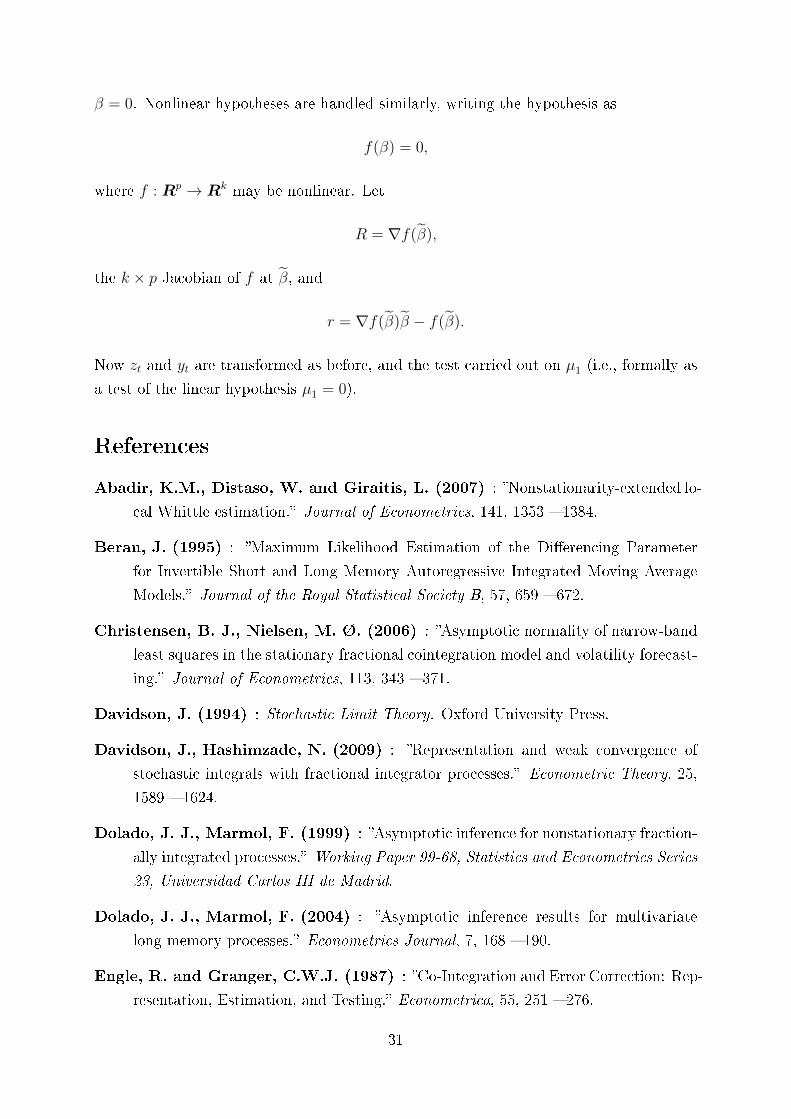
β = 0. Nonlinear hypotheses are handled similarly, writing the hypothesis as
f(β) = 0,
where f : Rp → Rk may be nonlinear. Let
R = ∇f(β),
the k × p Jacobian of f at β, and
r = ∇f(β)β − f(β).
Now zt and yt are transformed as before, and the test carried out on µ1 (i.e., formally as
a test of the linear hypothesis µ1 = 0).
References
Abadir, K.M., Distaso, W. and Giraitis, L. (2007) : �Nonstationarity-extended lo-
cal Whittle estimation.� Journal of Econometrics, 141, 1353 � 1384.
Beran, J. (1995) : �Maximum Likelihood Estimation of the Di�erencing Parameter
for Invertible Short and Long Memory Autoregressive Integrated Moving Average
Models.� Journal of the Royal Statistical Society B, 57, 659 � 672.
Christensen, B. J., Nielsen, M. Ø. (2006) : �Asymptotic normality of narrow-band
least squares in the stationary fractional cointegration model and volatility forecast-
ing.� Journal of Econometrics, 113, 343 � 371.
Davidson, J. (1994) : Stochastic Limit Theory. Oxford University Press.
Davidson, J., Hashimzade, N. (2009) : �Representation and weak convergence of
stochastic integrals with fractional integrator processes.� Econometric Theory, 25,
1589 � 1624.
Dolado, J. J., Marmol, F. (1999) : �Asymptotic inference for nonstationary fraction-
ally integrated processes.� Working Paper 99-68, Statistics and Econometrics Series
23, Universidad Carlos III de Madrid.
Dolado, J. J., Marmol, F. (2004) : �Asymptotic inference results for multivariate
long-memory processes.� Econometrics Journal, 7, 168 � 190.
Engle, R. and Granger, C.W.J. (1987) : �Co-Integration and Error Correction: Rep-
resentation, Estimation, and Testing.� Econometrica, 55, 251 � 276.
31
Geweke, J., Porter-Hudak, S. (1983) : �The estimation and application of long mem-
ory time series models.� Journal of Time Series Analysis, 4, 221 � 238.
Harris, P., Peers, H.W. (1980) : �The local power of the e�cient scores test statis-
tic.� Biometrika, 67, 525 � 529.
Harvey, D.I. and Leybourne, S.J. (2007) : Testing for time series linearity. Econo-
metrics Journal, 10, 149 � 165.
Harvey, D.I., Leybourne, S.J. and Taylor, A.M.R. (2009) : �Simple, robust and
powerful tests of the breaking trend hypothesis.� Econometric Theory, 25, 995 �
1029.
Harvey, D.I., Leybourne, S.J. and Xiao, L. (2010) : �Testing for nonlinear deter-
ministic components when the order of integration is unknown. � Journal of Time
Series Analysis, 31, 379 � 391.
Iacone, F., Leybourne, S.J. and Taylor, A.M.R. (2013a) : �On the behaviour of
�xed-b trend break tests under fractional integration.� Econometric Theory, 29, 393
� 418.
Iacone, F., Leybourne, S.J. and Taylor, A.M.R. (2013b) : �Testing for a break in
trend when the order of integration is unknown.� Journal of Econometrics, 176, 30
� 45.
Jansson, M. and Nielsen, M. Ø. (2012) : �Nearly e�cient likelihood ratio tests of
the unit root hypothesis.� Econometrica, 80, 2321 � 2332.
Johansen, M. and Nielsen, M. Ø. (2013) : �The role of initial values in nonstation-
ary fractional time series models.� Working Paper, Queens University.
Kim, C. S., and Phillips, P. C. B. (2001) : �Fully Modi�ed Estimation of Fractional
Cointegration Models. � Preprint, Yale University.
Marinucci, D. and Robinson, P. (1999) : �Alternative forms of fractional Brownian
motion.� Journal of Statistical Planning and Inference, 80, 111 � 122.
Nielsen, M. Ø. (2004) : �Optimal residual-based tests for fractional cointegration and
exchange rate dynamics.� Journal of Business and Economic Statistics, 22, 331 �
345.
Nielsen, M. Ø. (2007) : �Local Whittle Analysis of Stationary Fractional Cointegra-
tion and the Implied - Realized Volatility Relation.� Journal of Business and Eco-
nomics Statistics, 25, 427 � 446.
32

Perron, P., and Yabu, T. (2009) : �Testing for Shifts in Trend with an Integrated or
Stationary Noise Component.� Journal of Business and Economics Statistics, 27,
369 � 396.
Perron, P. and Zhu, X. (2005) : �Structural breaks with deterministic and stochastic
trends.� Journal of Econometrics, 129, 65 � 119.
Phillips, P.C.B. (1991) : �Optimal Inference in Cointegrated Systems.� Econometrica,
59, 283 � 306.
Phillips, P.C.B. and Hansen, B.E. (1990) : �Statistical Inference in Instrumental
Variables Regression With I(1) Processes.� Review of Economic Studies, 57, 99-125.
Rao, C.R. (1973) : Linear Statistical Inference and its Applications. Wiley, New York.
Robinson, P. M. (1994) : �E�cient Tests of Nonstationary Hypotheses.� Journal of
the American Statistical Association, 89, 1420 � 1437.
Robinson, P. M. (1995) : �Gaussian semiparametric estimation of long range depen-
dence.� Annals of Statistics, 23, 1048 � 1072.
Robinson, P. M. and Hualde, J. (2003) : �Cointegration in fractional systems with
unknown integration orders.� Econometrica, 71, 1727 � 1766.
Shimotsu, K. and Phillips, P.C.B. (2005) : �Exact local Whittle estimation of frac-
tional integration.� Annals of Statistics, 33, 1890 � 1933.
Shimotsu, K. (2010) : �Exact local Whittle estimation of fractional integration with
unknown mean and time trend.� Econometric Theory, 26, 501 � 540.
Sowell, F. (1990) : �The fractional unit root distribution.� Econometrica, 58, 495 �
505.
Vogelsang, T.J. (1998a) : �Trend function hypothesis testing in the presence of serial
correlation.� Econometrica, 66, 123 � 148.
Vogelsang, T.J. (1998b) : �Testing for a shift in mean without having to estimate
serial-correlation parameters.� Journal of Business and Economic Statistics, 16, 73
� 80.
Xu, J. and Perron, P. (2013) : �Robust testing of time trend and mean with unknown
integration order errors.� Working Paper, Boston University.
Zambrano, E. and Vogelsang, T.J. (2000) : �A simple test of the law of demand for
the United States.� Econometrica, 68, 1011 � 1020.
33


