A test of hypotheses for random graph distributions

built from EEG data

Andressa Cerqueira, Daniel Fraiman,

Claudia D. Vargas and Florencia Leonardi

April 27, 2015

Abstract

The theory of random graphs is being applied in recent years to model neural

interactions in the brain. While the probabilistic properties of random graphs has

been extensively studied in the literature, the development of statistical inference

methods for this class of objects has received less attention. In this work we pro-

pose a non-parametric test of hypotheses to test if two samples of random graphs

were originated from the same probability distribution. We show how to compute

efficiently the test statistic and we study its performance on simulated data. We

apply the test to compare graphs of brain functional network interactions built from

eletroencephalographic (EEG) data collected during the visualization of point light

displays depicting human locomotion.

1 Introduction

The brain consists in a complex network of interconnected regions whose functional inter-

play is thought to play a major role in cognitive processes [2, 14, 22]. Based on an elegant

representation of nodes (vertices) and links (edges) between pairs of nodes where nodes

usually represent anatomically defined brain regions while links represent functional or

effective connectivity [7], random graph theory is progressively allowing to explore prop-

erties of this sophisticated network [9, 13]. Such properties have been used so far to infer,

for instance, about effects of brain lesion [23], ageing [1, 24, 17] and neuropsychiatric

diseases (for a recent review, see [4]).

From a theoretical point of view, the most famous model of random graphs is the

Erdos-Reny model [12] (introduced by Gilbert in [15]), where the edges of the graphs are

independent and identically distributed Bernoulli random variables. Besides its simplicity,

this model continues to be actively studied and new properties are being discovered (see

1

arX

iv:1

504.

0647

8v1

[st

at.A

P] 2

4 A

pr 2

015

for example [11] and references therein). From the applied point of view the most popular

model is the Exponential Random Graph Model (ERGM) that has emerged mainly in the

Social Sciences community (see [19] and references therein).

Notwithstanding the crescent interest of the scientific community in the graph the-

ory applications, the development of statistical techniques to compare sets of graphs or

network data is still quite limited. Some recent works have addressed the problem of

maximum likelihood estimation in ERGM ([19, 21, 10]), but the testing problem has been

even less developed. As far as we know, the testing problem is restricted only to the

identification of differences in some one dimensional graph property ([13, 5, 3]). At this

point it is important to remark that the number of different graphs with v nodes grows as

fast as 2v(v−1)/2 which in practice is far much larger than a typical sample size analyzed.

This is the reason why the testing problem is difficult and relevant given that the graph

space has no total order.

In this paper we propose a goodness-of-fit test of hypothesis for random graph dis-

tributions. The statistic is inspired in a recent work [8] where a test of hypothesis for

random trees is developed. We show how to compute the test statistic efficiently and we

prove a Central Limit Theorem. The test makes no assumption on the specific form of

the distributions and it is consistent against any alternative hypothesis that differs form

the sample distribution on at least one edge-marginal. In a simulation study we show

the efficiency of the test and we compare its performance with the simultaneous testing

of the edge-marginals. We also apply the test to compare graphs built from electroen-

cephalographic (EEG) signals collected during the observation of videos depicting human

locomotion.

2 Definition of the test

Let V denote a finite set of vertices, with cardinal |V | = v, and let G(V ) denote the set

of all simple undirected graphs over V . We identify a graph g = (V,E) with the indicator

function gij = 1{(i, j) ∈ E}. Given a graph g ∈ G(V ), we denote by 1 − g the graph

defined by (1− g)ij = 1− gij.In order to measure a discrepancy between two graphs g, g′ ∈ G(V ) we introduce a

distance given by

D(g, g′) =∑ij

(gij − g′ij)2 .

Here and throughout the rest of the paper summations will refer to the set of vertices

(i, j) ∈ V 2 such that i < j (because gij = gji).

Given a set of graphs g = (g1, . . . , gn) and a graph g ∈ G(V ), we denote by Dg(g) the

2

mean distance of graph g to the set g; that is

Dg(g) =1

n

n∑k=1

D(g, gk) .

We also define the function g : V 2 → [0, 1], the mean of g, by

gij =1

n

n∑k=1

gkij .

Assume g is a random graph with distribution π. Denote by πij = π(gij = 1) and let

Σ denote the covariance matrix of π. Given another probability distribution π′ defined

on G(V ), we are interested in testing the hypothesis

H0 : π = π′ versus HA : π 6= π′ . (2.1)

Given an i.i.d sample of graphs g = (g1, . . . , gn) with distribution π, we define the one-

sample test statistic

W (g) = maxg∈G(V )

|Dg(g)− π′D(g, ·) | , (2.2)

where π′D(g, ·) denotes the mean distance of graph g to a random graph with distribution

π′ and is given by

π′D(g, ·) =∑

g′∈G(V )

D(g, g′)π′(g′) .

In the same way, given two samples g = (g1, . . . , gn) and g′ = (g′1, . . . , g′m) with

distributions π and π′ respectively, we define the two-sample test statistic

W (g,g′) = maxg∈G(V )

|Dg(g)− Dg′(g) | . (2.3)

At first sight the computation of (2.2) or (2.3) is prohibited for even a small number

of vertices. But as we show in the following proposition, it is possible to compute the test

statistic in O(v2(n+m)) time.

Proposition 2.1. For the one-sample test statistic we have that

W (g) =∑ij

∣∣gij − π′ij ∣∣ . (2.4)

Analogously, for the two-sample test statistic we have that

W (g,g′) =∑ij

∣∣gij − g′ij∣∣ . (2.5)

As a corollary of this proposition we prove the following result about the asymptotic

distribution of the test statistic. Let Π = (πij), Π = (gij) and Π′ = (g′ij). Then we can

write W (g) = ‖Π − Π‖ and W (g,g′) = ‖Π − Π′‖, where ‖ · ‖ denotes the vectorized

1-norm.

3

Corollary 2.2. Under H0, for the one-sample test statistic we have that

√n(Π− Π

) D−−−→n→∞

N(0,Σ) .

Analogously, for the two-sample test statistic we have that√nm

n+m

(Π− Π′

) D−−−−→n,m→∞

N(0,Σ) .

The proofs of these results are postponed to the Appendix.

Assuming the distribution of W under the null hypothesis is known, the result of the

test (2.1) at the significance level α is

Reject H0 if W (g) > q1−α ,

where q1−α is the (1−α)-quantile of the distribution of W under the null hypothesis. The

result of the test for the two-sample case is obtained in the same way replacing W (g) by

W (g,g′).

Remark 2.3. By the form of the resulting test statistic, given in (2.4) and (2.5), and

Corollary 2.2 we can deduce that the test is consistent against any alternative hypothesis

π′ with π′ij 6= πij for at least one pair ij.

3 Performance of the test on simulated data

In this section we present the results of a simulation study in order to evaluate the

performance of the test (2.1). In the first simulation example we compute the power

function of the one-sample test of a (modified) Erdos-Renyi model of parameter p ∈ (0, 1)

with v = 10 vertices, taking as null hypothesis the classical Erdos-Renyi model with

p0 = 0.5. In the modified model, a percentage q of the edges of the graph (previously

chosen) are independent Bernoulli variables with parameter p, and the remaining edges

are taken with parameter p0 as in the null model. The power function of the test (2.1)

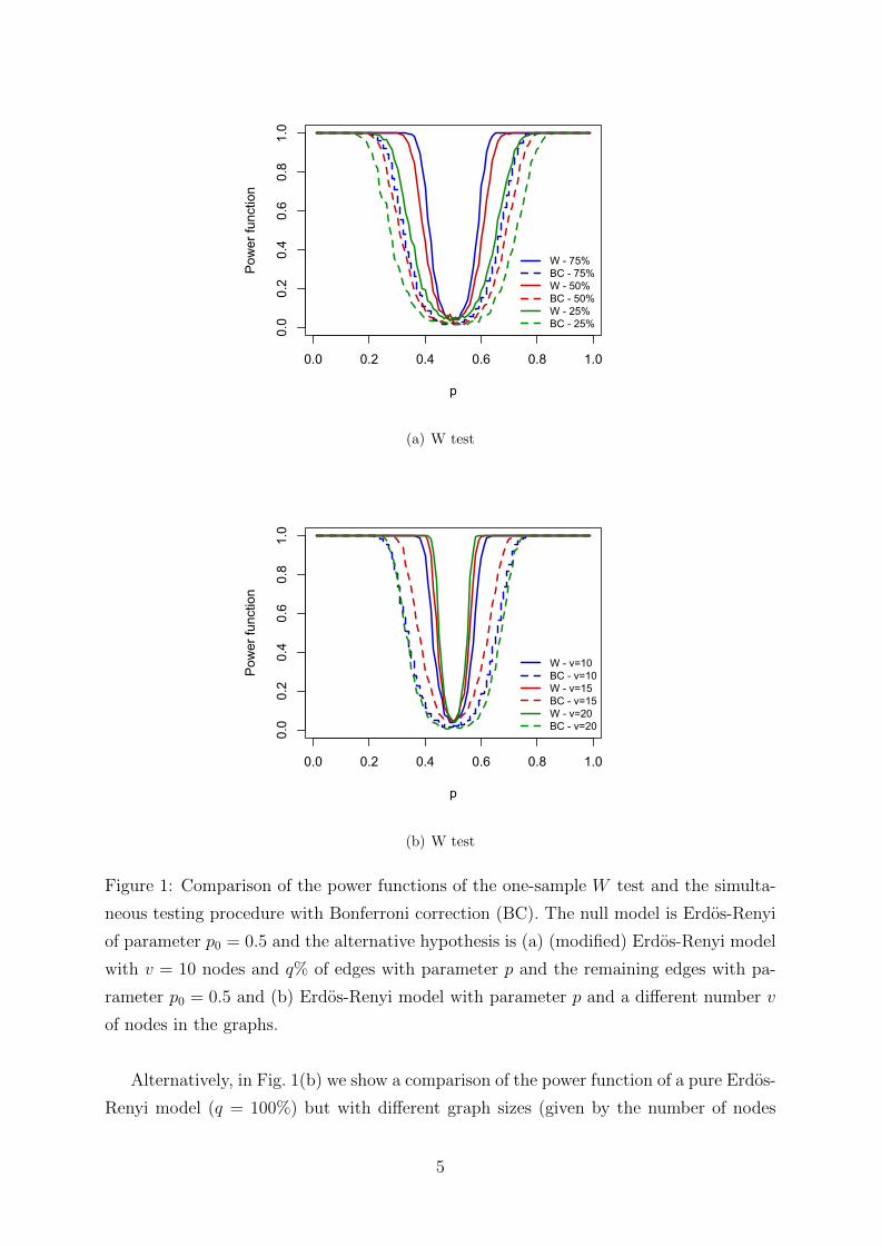
as a function of p and for different values of q is presented in Fig. 1(a). The sample size

was n = 20 and the quantile of the distribution of W (under H0) was computed as the

empirical 0.95 quantile of a simulation with p0 = 0.5 and 10.000 replications. Even for a

somehow small proportion of 25% of different edge probabilities and a small sample size

the test performs well and the power function approaches 1 when the absolute difference

|p − p0| grows. In order to compare our results with a classical method, we performed

simultaneous hypothesis tests on the edge occurrences by using Bonferroni correction

(BC). In this case exact critical regions were obtained from the Binomial distribution.

For all values of q, the W test performs better than the BC procedure, as shown in

Fig. 1(a).

4

0.0 0.2 0.4 0.6 0.8 1.0

0.0

0.2

0.4

0.6

0.8

1.0

p

Pow

er fu

nctio

nW - 75%BC - 75%W - 50%BC - 50%W - 25%BC - 25%

(a) W test

0.0 0.2 0.4 0.6 0.8 1.0

0.0

0.2

0.4

0.6

0.8

1.0

p

Pow

er fu

nctio

n

W - v=10BC - v=10W - v=15BC - v=15W - v=20BC - v=20

(b) W test

Figure 1: Comparison of the power functions of the one-sample W test and the simulta-

neous testing procedure with Bonferroni correction (BC). The null model is Erdos-Renyi

of parameter p0 = 0.5 and the alternative hypothesis is (a) (modified) Erdos-Renyi model

with v = 10 nodes and q% of edges with parameter p and the remaining edges with pa-

rameter p0 = 0.5 and (b) Erdos-Renyi model with parameter p and a different number v

of nodes in the graphs.

Alternatively, in Fig. 1(b) we show a comparison of the power function of a pure Erdos-

Renyi model (q = 100%) but with different graph sizes (given by the number of nodes

5

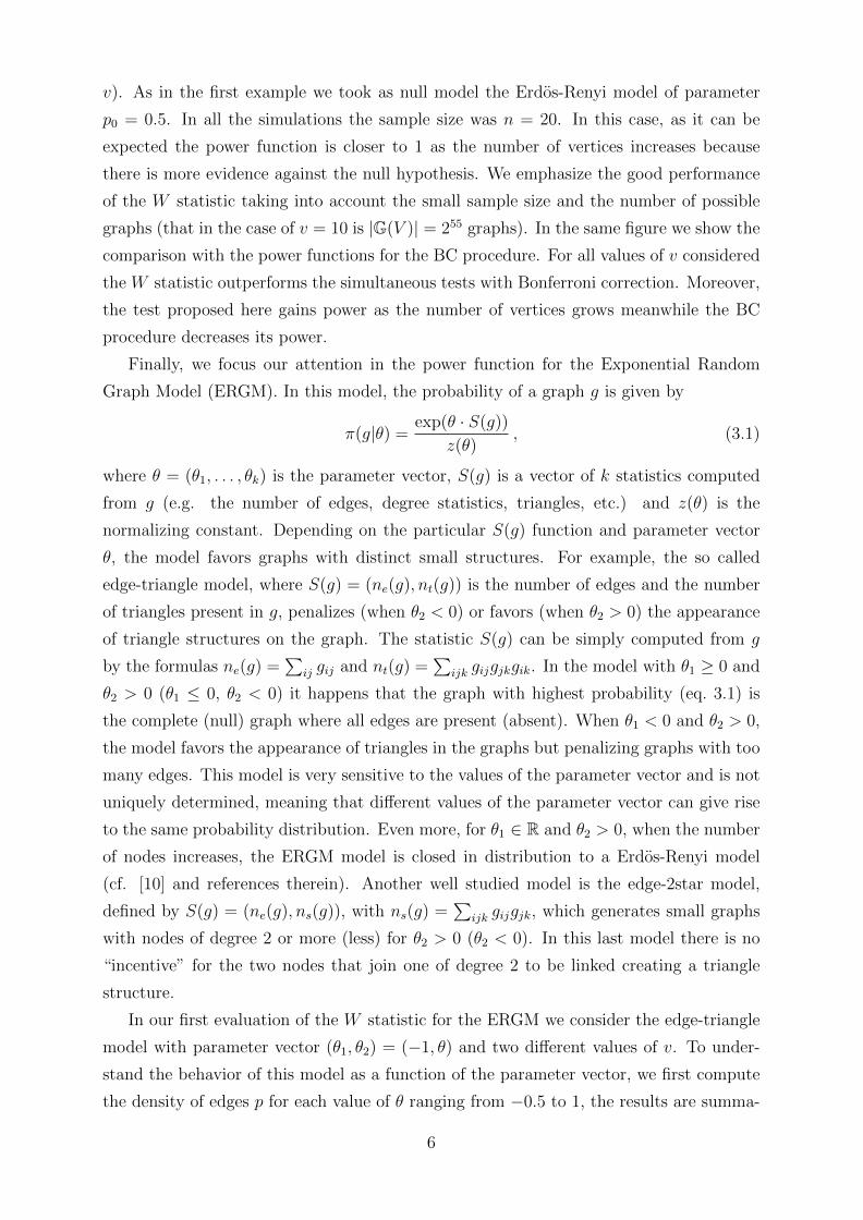
v). As in the first example we took as null model the Erdos-Renyi model of parameter

p0 = 0.5. In all the simulations the sample size was n = 20. In this case, as it can be

expected the power function is closer to 1 as the number of vertices increases because

there is more evidence against the null hypothesis. We emphasize the good performance

of the W statistic taking into account the small sample size and the number of possible

graphs (that in the case of v = 10 is |G(V )| = 255 graphs). In the same figure we show the

comparison with the power functions for the BC procedure. For all values of v considered

the W statistic outperforms the simultaneous tests with Bonferroni correction. Moreover,

the test proposed here gains power as the number of vertices grows meanwhile the BC

procedure decreases its power.

Finally, we focus our attention in the power function for the Exponential Random

Graph Model (ERGM). In this model, the probability of a graph g is given by

π(g|θ) =exp(θ · S(g))

z(θ), (3.1)

where θ = (θ1, . . . , θk) is the parameter vector, S(g) is a vector of k statistics computed

from g (e.g. the number of edges, degree statistics, triangles, etc.) and z(θ) is the

normalizing constant. Depending on the particular S(g) function and parameter vector

θ, the model favors graphs with distinct small structures. For example, the so called

edge-triangle model, where S(g) = (ne(g), nt(g)) is the number of edges and the number

of triangles present in g, penalizes (when θ2 < 0) or favors (when θ2 > 0) the appearance

of triangle structures on the graph. The statistic S(g) can be simply computed from g

by the formulas ne(g) =∑

ij gij and nt(g) =∑

ijk gijgjkgik. In the model with θ1 ≥ 0 and

θ2 > 0 (θ1 ≤ 0, θ2 < 0) it happens that the graph with highest probability (eq. 3.1) is

the complete (null) graph where all edges are present (absent). When θ1 < 0 and θ2 > 0,

the model favors the appearance of triangles in the graphs but penalizing graphs with too

many edges. This model is very sensitive to the values of the parameter vector and is not

uniquely determined, meaning that different values of the parameter vector can give rise

to the same probability distribution. Even more, for θ1 ∈ R and θ2 > 0, when the number

of nodes increases, the ERGM model is closed in distribution to a Erdos-Renyi model

(cf. [10] and references therein). Another well studied model is the edge-2star model,

defined by S(g) = (ne(g), ns(g)), with ns(g) =∑

ijk gijgjk, which generates small graphs

with nodes of degree 2 or more (less) for θ2 > 0 (θ2 < 0). In this last model there is no

“incentive” for the two nodes that join one of degree 2 to be linked creating a triangle

structure.

In our first evaluation of the W statistic for the ERGM we consider the edge-triangle

model with parameter vector (θ1, θ2) = (−1, θ) and two different values of v. To under-

stand the behavior of this model as a function of the parameter vector, we first compute

the density of edges p for each value of θ ranging from −0.5 to 1, the results are summa-

6

-0.5 0.0 0.5 1.0

0.0

0.2

0.4

0.6

0.8

1.0

θ

p

v=8v=12

0.4 0.6 0.8

0.0

0.2

0.4

0.6

0.8

1.0

v=8

θ

Pow

er fu

nctio

n

0.20 0.35 0.50

0.0

0.2

0.4

0.6

0.8

1.0

v=12

θ

Pow

er fu

nctio

n

(a) Edge-triange model

-0.6 -0.2 0.0 0.2 0.4 0.6

0.0

0.2

0.4

0.6

0.8

1.0

θ

p

v=8v=12

-0.1 0.2 0.4

0.0

0.2

0.4

0.6

0.8

1.0

v=8

θ

Pow

er fu

nctio

n

-0.1 0.1 0.3

0.0

0.2

0.4

0.6

0.8

1.0

v=12

θ

Pow

er fu

nctio

n

(b) Edge-2star model

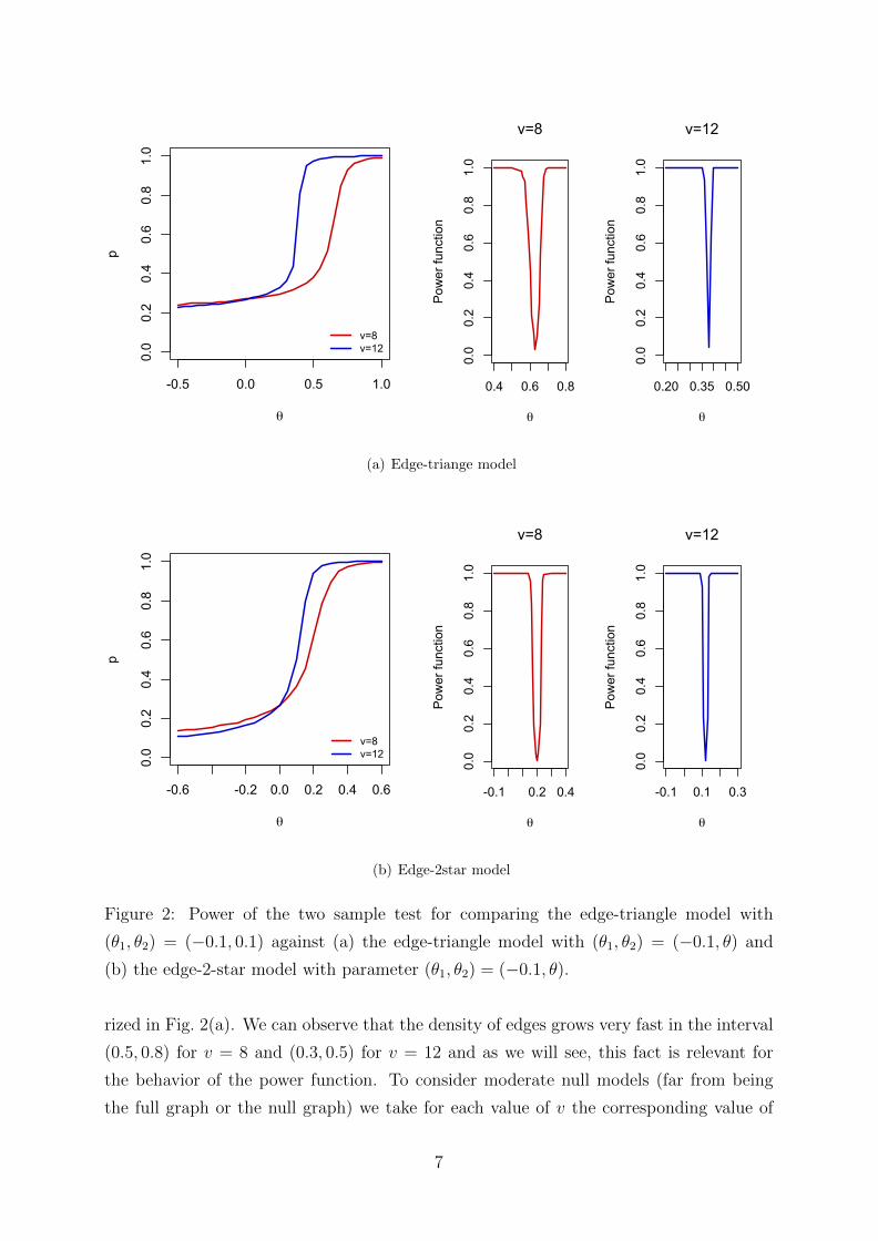
Figure 2: Power of the two sample test for comparing the edge-triangle model with

(θ1, θ2) = (−0.1, 0.1) against (a) the edge-triangle model with (θ1, θ2) = (−0.1, θ) and

(b) the edge-2-star model with parameter (θ1, θ2) = (−0.1, θ).

rized in Fig. 2(a). We can observe that the density of edges grows very fast in the interval

(0.5, 0.8) for v = 8 and (0.3, 0.5) for v = 12 and as we will see, this fact is relevant for

the behavior of the power function. To consider moderate null models (far from being

the full graph or the null graph) we take for each value of v the corresponding value of

7

θ given a density of edges approximately equal to p = 0.6, this corresponds to θ2 = 0.63

for v = 8 and θ2 = 0.38 for v = 12. For each one of these null models, we computed the

(1−α)-quantile of the distribution of W under H0 for the one sample test statistic (2.4),

using 2000 replications of W with sample size n = 20. Then we computed the power

function of the test against any hypothesis with θ2 = θ, with θ ranging from −0.5 to 1.

We can see that the power functions grow very fast to 1 and this is a consequence of θ2 in

the null model being in the interval where p grows very fast. The behavior of the power

function is very anomalous if we take as null model a value of θ2 belonging to a flat region

of p, because in these cases a big difference in θ does not imply a big difference in p, and

this is determinant for the value of the power function.

In our second example we took the same null models for each one of the two cases

v = 8 and v = 12 and computed the power function for the edge-2star model with

parameter vector (θ1, θ2) = (−1, θ), with θ varying between −0.6 and 0.6. As in our

previous example, we computed the density of edges p for each value of θ (Fig. 2(b)). In

these cases the power function also converges very fast to 1 because the value p = 0.6 of

the null hypothesis lies in a region where the density of edges in the edge-2star model also

grows very fast as a function of θ.

4 Discrimination of EEG brain networks

The data analyzed in this section where first presented in [20]. A total of sixteen healthy

subjects (29.25±6.3 years) with normal or corrected to normal vision and with no known

neurological abnormalities participated in this study. The study was conducted in accor-

dance with the declaration of Helsinki (1964) and approved by the local ethics committee

(Comite de Etica em pesquisa do Hospital Universitario Clementino Fraga Filho, Univer-

sidade Federal do Rio de Janeiro, 303.416).

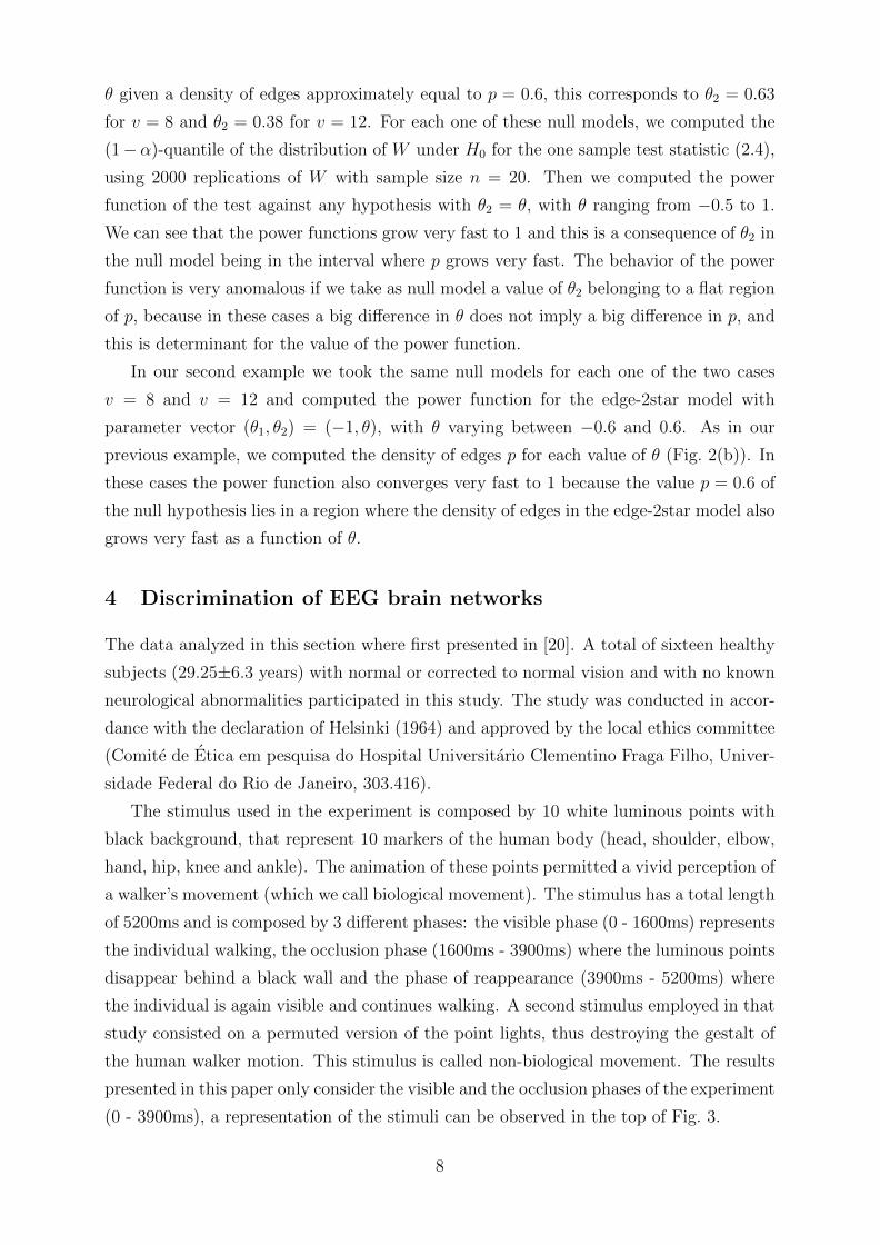
The stimulus used in the experiment is composed by 10 white luminous points with

black background, that represent 10 markers of the human body (head, shoulder, elbow,

hand, hip, knee and ankle). The animation of these points permitted a vivid perception of

a walker’s movement (which we call biological movement). The stimulus has a total length

of 5200ms and is composed by 3 different phases: the visible phase (0 - 1600ms) represents

the individual walking, the occlusion phase (1600ms - 3900ms) where the luminous points

disappear behind a black wall and the phase of reappearance (3900ms - 5200ms) where

the individual is again visible and continues walking. A second stimulus employed in that

study consisted on a permuted version of the point lights, thus destroying the gestalt of

the human walker motion. This stimulus is called non-biological movement. The results

presented in this paper only consider the visible and the occlusion phases of the experiment

(0 - 3900ms), a representation of the stimuli can be observed in the top of Fig. 3.

8

0

Visible

1600

Occlusion

3600 time (ms)

V1 V2 V3 V4 O1 O2 O3 O4

F7

T3

T5

Fp1

F3

C3

P3

O1

F8

T4

T6

Fp2

F4

C4

P4

O2

Fz

Cz

Pz

Oz

F7

T3

T5

Fp1

F3

C3

P3

O1

F8

T4

T6

Fp2

F4

C4

P4

O2

Fz

Cz

Pz

Oz

333ms

stimulus

EEG signal

inte

ract

ion

crit

erio

n

correlationmatrix

net

wor

kcr

iter

ion

graph

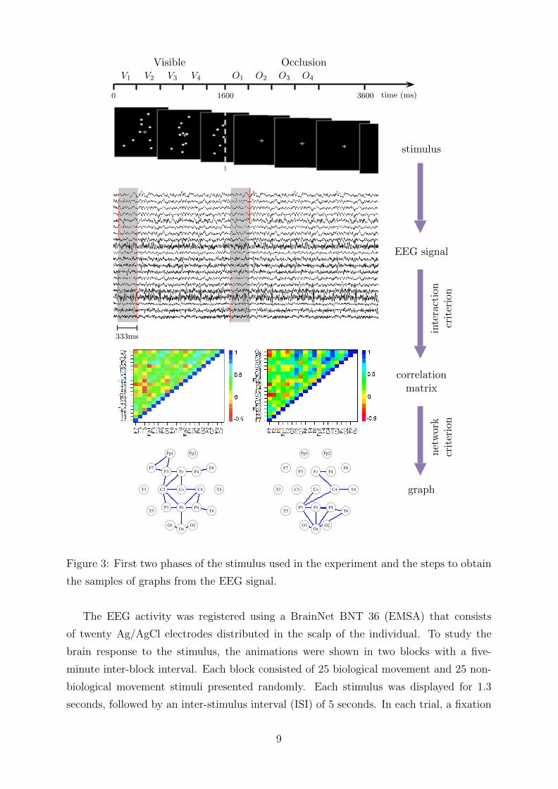
1Figure 3: First two phases of the stimulus used in the experiment and the steps to obtain

the samples of graphs from the EEG signal.

The EEG activity was registered using a BrainNet BNT 36 (EMSA) that consists

of twenty Ag/AgCl electrodes distributed in the scalp of the individual. To study the

brain response to the stimulus, the animations were shown in two blocks with a five-

minute inter-block interval. Each block consisted of 25 biological movement and 25 non-

biological movement stimuli presented randomly. Each stimulus was displayed for 1.3

seconds, followed by an inter-stimulus interval (ISI) of 5 seconds. In each trial, a fixation

9

cross appeared in the last second of the ISI. A total of 100 point light animations were

displayed (2 blocks, 2 conditions [biological and non-biological movement], 25 repetitions).

To construct the brain functional networks, for each subject, phase and repetition of

the experiment we first computed a Spearman correlation between each pair of electrodes

for each temporal window [t, t + 333ms], for values of t varying every 16.66ms (this cor-

responds to the interaction criterion in Fig. 3). The series of correlations for each pair

of electrodes ij (and specific for each subject, phase and repetition) will be denoted by

{ρijt : t = t1, . . . , tn}. For the construction of the graphs we computed a threshold for

each pair of electrodes ij based on this series of correlations and we put an edge between

these electrodes if the absolute value of the correlation for a given time t was above this

threshold (this step corresponds to the network criterion in Fig. 3). That means to say

that for each pair of electrodes we selected a different threshold value, and the selection

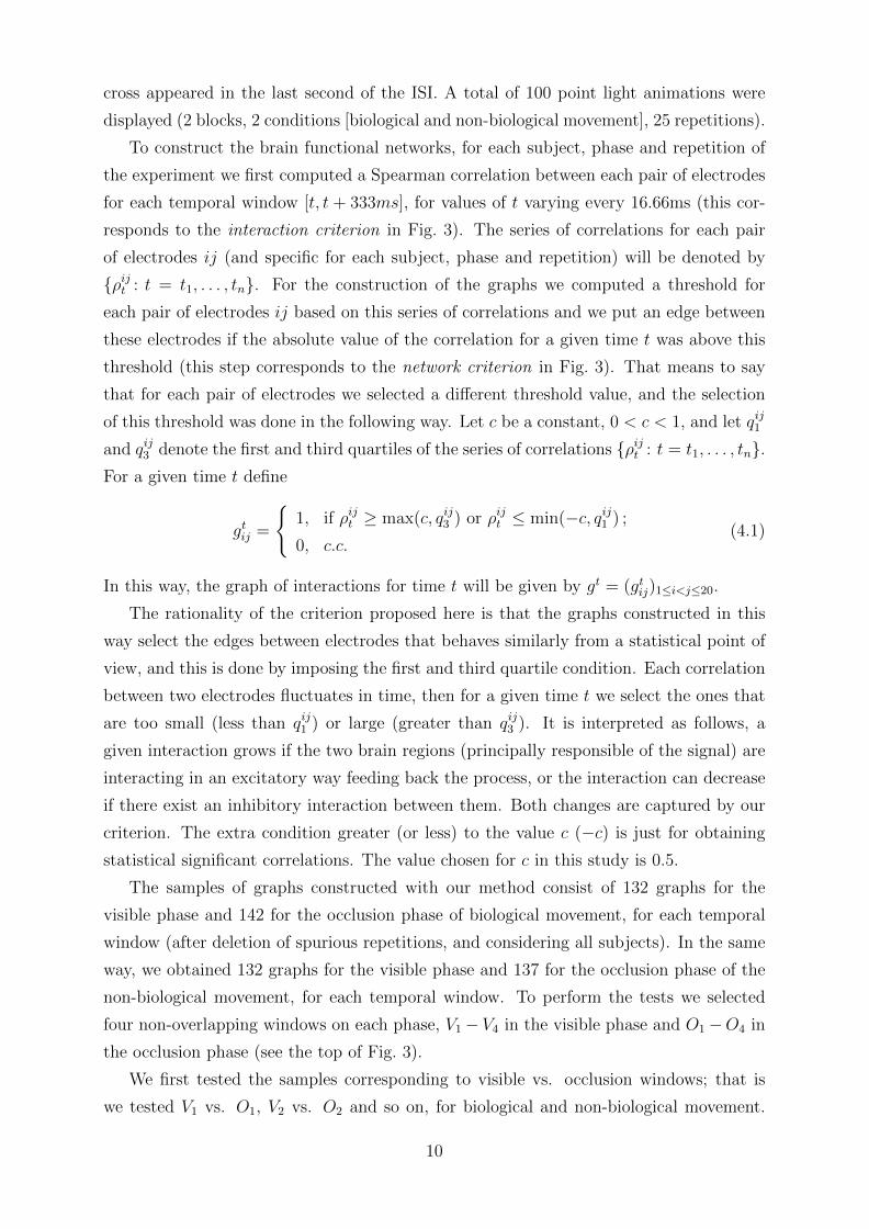
of this threshold was done in the following way. Let c be a constant, 0 < c < 1, and let qij1

and qij3 denote the first and third quartiles of the series of correlations {ρijt : t = t1, . . . , tn}.For a given time t define

gtij =

{1, if ρijt ≥ max(c, qij3 ) or ρijt ≤ min(−c, qij1 ) ;

0, c.c.(4.1)

In this way, the graph of interactions for time t will be given by gt = (gtij)1≤i<j≤20.

The rationality of the criterion proposed here is that the graphs constructed in this

way select the edges between electrodes that behaves similarly from a statistical point of

view, and this is done by imposing the first and third quartile condition. Each correlation

between two electrodes fluctuates in time, then for a given time t we select the ones that

are too small (less than qij1 ) or large (greater than qij3 ). It is interpreted as follows, a

given interaction grows if the two brain regions (principally responsible of the signal) are

interacting in an excitatory way feeding back the process, or the interaction can decrease

if there exist an inhibitory interaction between them. Both changes are captured by our

criterion. The extra condition greater (or less) to the value c (−c) is just for obtaining

statistical significant correlations. The value chosen for c in this study is 0.5.

The samples of graphs constructed with our method consist of 132 graphs for the

visible phase and 142 for the occlusion phase of biological movement, for each temporal

window (after deletion of spurious repetitions, and considering all subjects). In the same

way, we obtained 132 graphs for the visible phase and 137 for the occlusion phase of the

non-biological movement, for each temporal window. To perform the tests we selected

four non-overlapping windows on each phase, V1− V4 in the visible phase and O1−O4 in

the occlusion phase (see the top of Fig. 3).

We first tested the samples corresponding to visible vs. occlusion windows; that is

we tested V1 vs. O1, V2 vs. O2 and so on, for biological and non-biological movement.

10

Visible vs OcclusionWindows

V1 vs. O1 V2 vs. O2 V3 vs. O3 V4 vs. O4

Biological 0.0019 0.4294 0.1984 0.0278

Non-biological 0.0016 0.8278 0.1249 0.6673

(a) P -value of visible vs. occlusion phases.

F7

T3

T5

Fp1

F3

C3

P3

O1

F8

T4

T6

Fp2

F4

C4

P4

O2

Fz

CZ

Pz

Oz

F7

T3

T5

Fp1

F3

C3

P3

O1

F8

T4

T6

Fp2

F4

C4

P4

O2

Fz

CZ

Pz

Oz

(b) Summary graphs for biological movement.

F7

T3

T5

Fp1

F3

C3

P3

O1

F8

T4

T6

Fp2

F4

C4

P4

O2

Fz

CZ

Pz

Oz

F7

T3

T5

Fp1

F3

C3

P3

O1

F8

T4

T6

Fp2

F4

C4

P4

O2

Fz

CZ

Pz

Oz

(c) Summary graphs for non-biological movement.

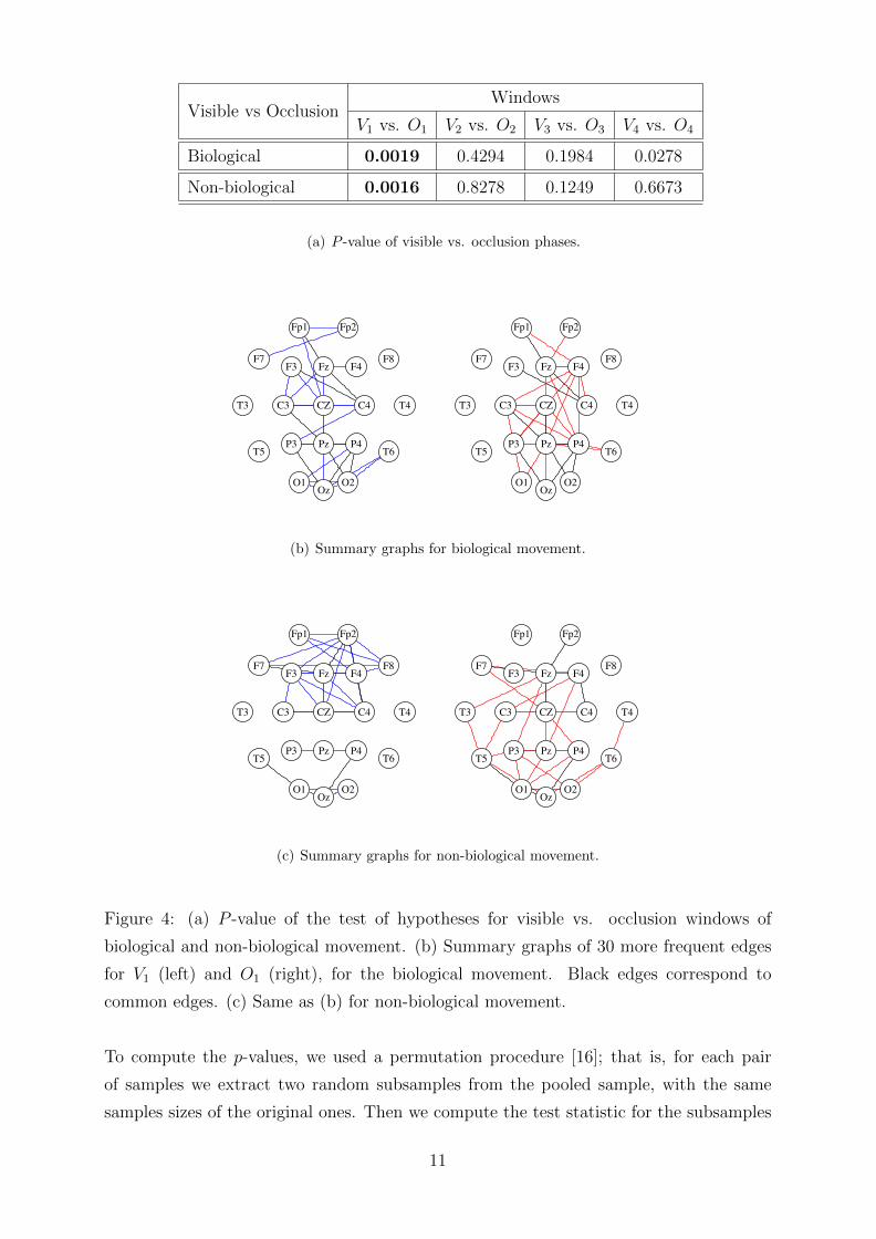
Figure 4: (a) P -value of the test of hypotheses for visible vs. occlusion windows of

biological and non-biological movement. (b) Summary graphs of 30 more frequent edges

for V1 (left) and O1 (right), for the biological movement. Black edges correspond to

common edges. (c) Same as (b) for non-biological movement.

To compute the p-values, we used a permutation procedure [16]; that is, for each pair

of samples we extract two random subsamples from the pooled sample, with the same

samples sizes of the original ones. Then we compute the test statistic for the subsamples

11

extracted in this way, and we replicate this procedure 1000 times. The estimated p-value

is therefore the empirical proportion of values in the vector of size 1000 built up in this

way that are greater than the observed W statistic. The p-values obtained for the four

tests are reported in Fig. 4(a). We notice that in both types of movement the p-values

corresponding to the first windows of visible and occlusion phases are significantly smaller

than the other p-values. The stimulus onset evokes an event related response [18] in the

first window of the visible phase. This response, also known as visual evoked potential, is

absent in the occlusion phase where there is no stimulus presentation. As can be observed

the W statistic is able to retrieve this difference from the graphs distributions.

It is important to remark that the test of hypotheses proposed here does not dis-

criminate which edges in the graphs contribute more significantly to distinguish the two

conditions under analysis. Therefore, to compile the results obtained with the test of

hypotheses we plotted a summary graph representing each sample by selecting the 30

more frequent edges. Fig. 4(b)-(c) illustrate the graphs corresponding to V1 and O1 in the

biological and non-biological movement conditions for which the smallest p-values were

found, as illustrated in Fig. 4(a).

Although the plots of the 30 most frequent edges in the first window of the visible and

occlusion phases are quite similar for the biological movement condition, comparatively

less edges seem present in the occipital electrodes (O1, Oz and O2) and there is a shift

towards the right parietofrontal region in the occlusion period. These results could be

taken as an evidence of the hypothesis raised in [20] that the brain would implicitly

“reenact” the observed biological movement during the occlusion period (see for more

details). For the non-biological condition, the 30 most frequent edges in the first window

of the visual phase clearly connect electrodes in the frontal region whereas the 30 most

frequent edges in the first window of the occlusion phase connect electrodes in the central-

occipital region.

Comparing the biological and non biological conditions during the visible phase,

Saunier et al. (2013) [20] found differences both in the right temporo-parietal and in

centro-frontal regions. Using functional connectivity, Fraiman et al. (2014) [13] con-

firmed that the left frontal regions may play a major role when it comes to discriminating

biological x non biological movements. To confirm these findings we proceeded to test the

corresponding windows of the biological and non-biological movement conditions. For the

visible phase the smallest p-value (< 0.03) was obtained for the third temporal window

(time between 668.3ms and 1001.7ms). The occlusion phase does not report significant

results in any of the tested windows, see Fig. 5. We emphasize the fact that this is a

more sensible problem compared to the comparison of visible and occlusion windows, in

the sense that the differences in the stimuli are very subtle. For that reason it is not

surprising that with the actual sample sizes we do not obtain very significant results in

12

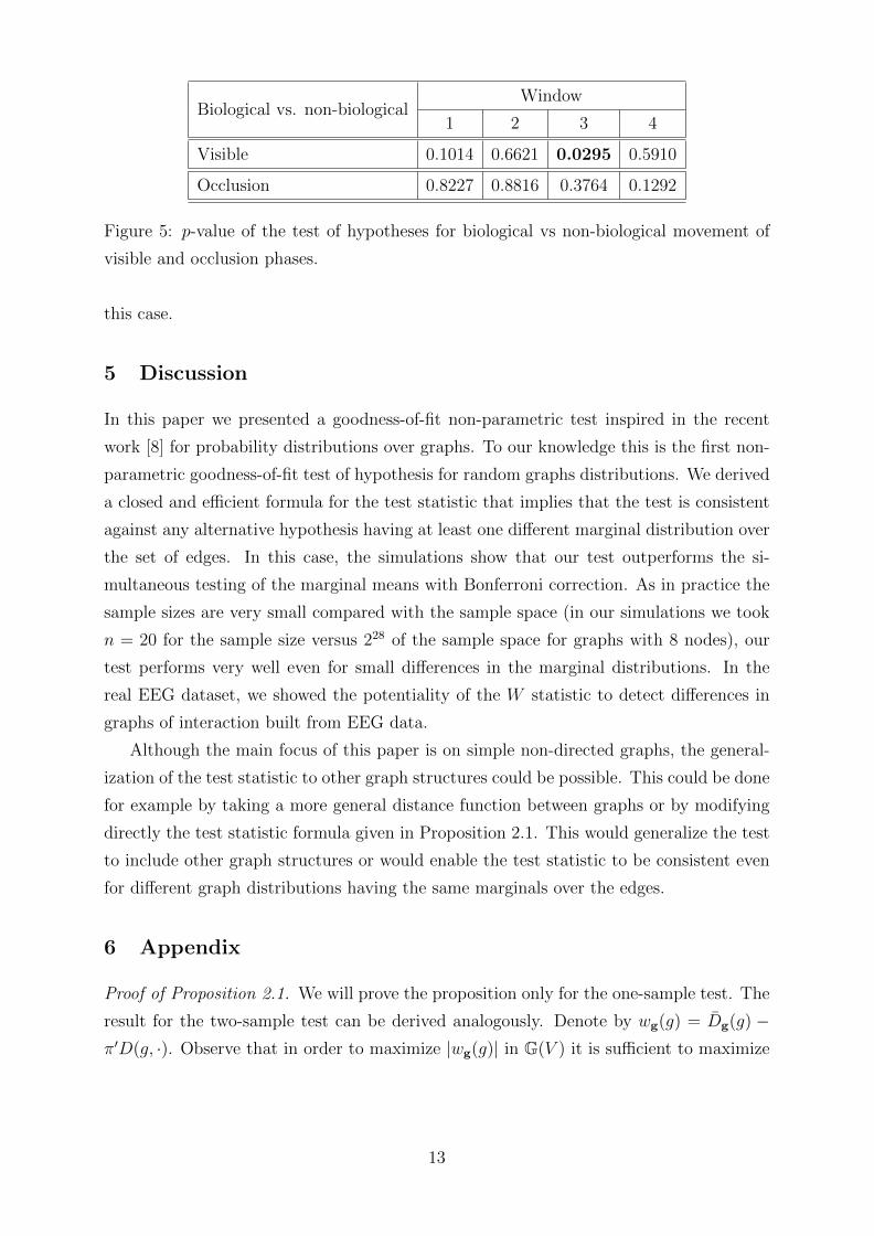
Biological vs. non-biologicalWindow

1 2 3 4

Visible 0.1014 0.6621 0.0295 0.5910

Occlusion 0.8227 0.8816 0.3764 0.1292

Figure 5: p-value of the test of hypotheses for biological vs non-biological movement of

visible and occlusion phases.

this case.

5 Discussion

In this paper we presented a goodness-of-fit non-parametric test inspired in the recent

work [8] for probability distributions over graphs. To our knowledge this is the first non-

parametric goodness-of-fit test of hypothesis for random graphs distributions. We derived

a closed and efficient formula for the test statistic that implies that the test is consistent

against any alternative hypothesis having at least one different marginal distribution over

the set of edges. In this case, the simulations show that our test outperforms the si-

multaneous testing of the marginal means with Bonferroni correction. As in practice the

sample sizes are very small compared with the sample space (in our simulations we took

n = 20 for the sample size versus 228 of the sample space for graphs with 8 nodes), our

test performs very well even for small differences in the marginal distributions. In the

real EEG dataset, we showed the potentiality of the W statistic to detect differences in

graphs of interaction built from EEG data.

Although the main focus of this paper is on simple non-directed graphs, the general-

ization of the test statistic to other graph structures could be possible. This could be done

for example by taking a more general distance function between graphs or by modifying

directly the test statistic formula given in Proposition 2.1. This would generalize the test

to include other graph structures or would enable the test statistic to be consistent even

for different graph distributions having the same marginals over the edges.

6 Appendix

Proof of Proposition 2.1. We will prove the proposition only for the one-sample test. The

result for the two-sample test can be derived analogously. Denote by wg(g) = Dg(g) −π′D(g, ·). Observe that in order to maximize |wg(g)| in G(V ) it is sufficient to maximize

13

wg(g) and −wg(g). We have that

wg(g) =1

n

n∑k=1

D(g, gk)−∑

g′∈G(V )

D(g, g′)π′(g′) .

The first sum equals

1

n

n∑k=1

D(g, gk) =1

n

n∑k=1

∑ij

(gij − gkij)2

=∑ij

(gij − 2gijgij + gij) .

The second sum is ∑g′∈G(V )

D(g, g′)π′(g′) =∑

g′∈G(V )

π′(g′)∑ij

(gij − g′ij)2

=∑ij

(gij − 2gijπ′ij + π′ij) .

Therefore we have that

wg(g) =∑ij

(2gij − 1)(π′ij − gij) . (6.1)

As this is a weighted sum, the graph g∗ ∈ G(V ) that maximizes wg(g) is given by

g∗ij =

1, if gij ≤ π′ij

0, c.c.(6.2)

Similarly, the graph g∗∗ ∈ G(V ) that maximizes −wg(g) is given by

g∗∗ij =

1, if gij ≥ π′ij

0, c.c.(6.3)

Note also that by a direct calculation from (6.1) and the definitions (6.2) and (6.3) we

have that |wg(g)| = | − wg(g)|. Finally, from (2.4) and (6.2) we obtain

W (g) = maxg∈G(V )

|wg(g)| = wg(g∗) =∑ij

|gij − π′ij| .

Proof of Corollary 2.2. This is a direct consequence of the multidimensional Central Limit

Theorem (cf. Theorem 11.10 in [6]).

Acknowledgments

F.L. is partially supported by a CNPq-Brazil fellowship (304836/2012-5) and FAPESP’s

fellowship (2014/00947-0). This article was produced as part of the activities of FAPESP

Research, Innovation and Dissemination Center for Neuromathematics, grant 2013/07699-

0, Sao Paulo Research Foundation. She also thanks L’Oreal Foundation for a “Women in

Science” grant.

14

References

[1] S. Achard and E. Bullmore. Efficiency and cost of economical brain functional net-

works. PLoS Computational Biology, 3:174—-183, 2007.

[2] A. Aertsen, G. Gerstein, M. Habib, and G. Palm. Dynamics of neuronal firing corre-

lation: modulation of” effective connectivity. Journal of neurophysiology, 61:900–917,

1989.

[3] P. Barttfeld, A. Petroni, S. Baez, H. Urquina, M. Sigman, M. Cetkovich, T. Torralva,

F. Torrente, A. Lischinsky, X. Castellanos, F. Manes, and A. Ibanez. Functional

connectivity and temporal variability of brain connections in adults with attention

deficit/hyperactivity disorder and bipolar disorder. Neuropsychobiology, 69:65–75,

2014.

[4] D. Bassett and E. Bullmore. Human brain networks in health and disease. Current

opinion in neurology, 22:340–347, 2009.

[5] M. Boersma, D. Smit, H. de Bie, C. Van Baal, D. Boomsma, E. de Geus,

H. Delemarre-van de Wall, and C. Stam. Network analysis of resting state eeg in

the developing young brain: Structure comes with maturation. Hum. Brain Mapp.,

32:413–425, 2011.

[6] L. Breiman. Probability, volume 7 of Classics in Applied Mathematics. Society for

Industrial and Applied Mathematics (SIAM), Philadelphia, PA, 1992. Corrected

reprint of the 1968 original.

[7] E. Bullmore and O. Sporns. Complex brain networks: graph theoretical analysis

of structural and functional systems. Nature Reviews Neuroscience, 10(3):186–198,

February 2009.

[8] J.R. Busch, P.A. Ferrari, A.G. Flesia, R. Fraiman, S.P. Grynberg, and F. Leonardi.

Testing statistical hypothesis on random trees and applications to the protein clas-

sification problem. Ann. Appl. Stat., 3(2):542–563, 2009.

[9] C. Calmels, M. Foutren, and C. Stam. Beta functional connectivity modulation

during the maintenance of motion information in working memory: importance of

the familiarity of the visual context. Neuroscience, 212:49–58, 2012.

[10] S. Chatterjee and P. Diaconis. Estimating and understanding exponential random

graph models. Ann. Statist., 41(5):2428–2461, 2013.

15

[11] S. Chatterjee and S.R.S. Varadhan. The large deviation principle for the Erdos-Renyi

random graph. European J. Combin., 32(7):1000–1017, 2011.

[12] P. Erdos and A. Renyi. On the evolution of random graphs. Magyar Tud. Akad.

Mat. Kutato Int. Kozl., 5:17–61, 1960.

[13] D. Fraiman, G. Saunier, E. Martins, and C. Vargas. Biological motion coding in the

brain: analysis of visually-driven eeg funcional networks. Plos One., page 0084612,

2014.

[14] K. Friston, P. Frith, P. add Liddle, and R. Frackowiak. Functional connectivity: the

principal-component analysis of large (pet) data sets. Journal of cerebral blood flow

and metabolism, 13:5–14, 1993.

[15] E. N. Gilbert. Random graphs. Ann. Math. Statist., 30:1141–1144, 1959.

[16] B.F.J. Manly. Randomization, bootstrap and Monte Carlo methods in biology. Chap-

man & Hall/CRC Texts in Statistical Science Series. Chapman & Hall/CRC, Boca

Raton, FL, third edition, 2007.

[17] D. Meunier, S. Achard, A. Morcom, and E. Bullmore. Age-related changes in modular

organization of human brain functional networks. Neuroimage, 44:715–723, 2009.

[18] T.W. Picton, S. Bentin, P. Berg, E. Donchin, S.A. Hillyard, R. Johnson, G.A. Miller,

W. Ritter, D.S. Ruchkin, M.D. Rugg, and M.J. Taylor. Guidelines for using human

event-related potentials to study cognition: Recording standards and publication

criteria. Psychophysiology, 37:127–152, 3 2000.

[19] A. Rinaldo, S.E. Fienberg, and Y. Zhou. On the geometry of discrete exponential

families with application to exponential random graph models. Electron. J. Stat.,

3:446–484, 2009.

[20] G. Saunier, E.F. Martins, E.C. Dias, J.M. de Oliveira, T. Pozzo, and C.D. Var-

gas. Electrophysiological correlates of biological motion permanence in humans. Be-

havioural Brain Research, 236:166–174, 2013.

[21] T.A. B. Snijders, J. Koskinen, and M. Schweinberger. Maximum likelihood estimation

for social network dynamics. Ann. Appl. Stat., 4(2):567–588, 2010.

[22] M. Van Den Heuvel and H. Pol. Exploring the brain network: a review on resting-

state fmri functional connectivity. European Neuropsychopharmacology, 8:519–534,

2010.

16

[23] L. Wang, C. Yu, H. Chen, W. Qin, Y. He, F. Fan, Zhang W., Wang M., K. Li,

Y. Zang, T. Woodward, and C. Zhu. Dynamic functional reorganization of the motor

execution network after stroke. Brain, 133:1224–1238, 2010.

[24] T. Wu, Y. Zang, L. Wang, X. Long, M. Hallett, Y. Chen, L. Kuncheng, and P. Chan.

Aging influence on functional connectivity of the motor network in the resting state.

Neuroscience letters, 422:164–168, 2007.

17