A statistical approach for polarized parton distributions

Digital Object Identifier (DOI) 10.1007/s100520100855Eur. Phys. J. C 23, 487–501 (2002) THE EUROPEAN

PHYSICAL JOURNAL C

A statistical approach for polarized parton distributions

C. Bourrely1, J. Soffer1, F. Buccella2,∗

1 Centre de Physique Theoriquea, CNRS-Luminy Case 907, 13288 Marseille Cedex 9, France2 Dipartimento di Scienze Fisiche, Universita di Napoli, Via Cintia, 80126 Napoli, Italy

Received: 19 September 2001 /Published online: 8 March 2002 – c© Springer-Verlag / Societa Italiana di Fisica 2002

Abstract. A global next-to-leading order QCD analysis of unpolarized and polarized deep-inelastic scatter-ing data is performed with parton distributions constructed in a statistical physical picture of the nucleon.The chiral properties of QCD lead to strong relations between quarks and antiquarks distributions and theimportance of the Pauli exclusion principle is also emphasized. We obtain a good description, in a broadrange of x and Q2, of all measured structure functions in terms of very few free parameters. We stress thefact that at RHIC-BNL the ratio of the unpolarized cross sections for the production of W+ and W − inpp collisions will directly probe the behavior of the d(x)/u(x) ratio for x ≥ 0.2, a definite and importanttest for the statistical model. Finally, we give specific predictions for various helicity asymmetries for theW ±, Z production in pp collisions at high energies, which will be measured with forthcoming experimentsat RHIC-BNL and which are sensitive tests of the statistical model for ∆u(x) and ∆d(x).

1 Introduction

Deep-inelastic scattering (DIS) of leptons on hadrons hasbeen extensively studied, over the last twenty years orso, both theoretically and experimentally. The principalgoals of this physics program were, first, to elucidate theinternal proton structure, in terms of parton distributions,and more recently to test perturbative quantum chromo-dynamics (QCD), which generalizes the parton model.For the unpolarized structure functions, the advent of theHERA physics program gives us access to a broader kine-matic range than fixed targets experiments, in x downto a few 10−5 and in Q2 up to several 104 GeV2, whichallows for testing perturbative QCD to next-to-leadingorder (NLO). As a result, the unpolarized light quarks(u, d) distributions are fairly well determined. Moreover,the data exhibit clear evidence for a flavor-asymmetriclight sea, i.e. d > u, which can be understood in termsof the Pauli exclusion principle, based on the fact thatthe proton contains two u quarks and only one d quark[1]. Larger uncertainties still persist for the gluon (G) andthe heavy quarks’ (s, c) distributions. From the more re-stricted amount of data on polarized structure functions,the corresponding polarized gluon and s quark distribu-tions (∆G,∆s) are badly constrained and we just beginto uncover a flavor asymmetry, for the corresponding po-larized light sea, namely ∆u �= ∆d. Whereas the signs ofthe polarized light quarks distributions are essentially wellestablished, ∆u > 0 and ∆d < 0, this is not the case for∆u and ∆d. The objective of this paper is to construct

a Unite Propre de Recherche 7061∗ Supported by INFN, Sezione di Napoli, Italy

a complete set of polarized parton (all flavor quarks, an-tiquarks and gluon) distributions; and, in particular, wewill try to clarify this last point on the polarized light sea.

The polarized parton distributions (PPD) of the nu-cleon have been extensively studied in the last few years[2,3] and in most models, the PPD are constructed from aset of unpolarized parton distributions, previously deter-mined, from unpolarized DIS data. For example for eachquark flavor qi(x), the corresponding ∆qi(x) is taken (atthe input energy scale) such that

∆qi(x) = ai(x) · qi(x), (1)

where ai(x) is a simple polynomial which has to be de-termined from the polarized DIS data. A similar proce-dure is used for antiquarks and gluons. As a result, thefull determination of all unpolarized and polarized partondistributions involves a large number of free parameters,say around 20–25, which obviously shows lack of simplic-ity. In addition, most of these models do not provide aflavor separation [4] for the antiquarks qi(x) and conse-quently for ∆qi(x). However, there are recent attemptsto make this flavor separation, either using semi-inclusivepolarized DIS data [5] or by means of a flavor-symmetrybreaking [6]. Our motivation for this work is to use thestatistical approach to build up qi, ∆qi, qi, ∆qi, G and∆G, by means of a very small number of free parameters.A flavor separation for the unpolarized and polarized lightsea is automatically achieved in a way dictated by our ap-proach.

This paper is organized as follows. In Sect. 2, we re-view the main points of our approach and we describe ourmethod to determine the free parameters of the PPD with

488 C. Bourrely et al.: A statistical approach for polarized parton distributions

the set of experimental data we have used. In Sect. 3, weshow the results obtained for the unpolarized DIS struc-ture functions F p,d

2 (x,Q2) and xF νN3 (x,Q2) in a wide

kinematic range, compared with the world data. We showthe prediction of the ratio of unpolarized W+ and W−cross section at RHIC-BNL, which is sensitive to thed(x)/u(x) ratio, a challenging question for the statisticalapproach. Section 4 is devoted to the polarized DIS struc-ture functions gp,d,n

1 (x,Q2). In Sect. 5, we give our predic-tions for single and double helicity asymmetries for theheavy gauge boson production (W±, Z) in pp collisions athigh energies, which are sensitive to ∆u and ∆d and willbe tested with forthcoming experiments at RHIC-BNL.We give our concluding remarks in Sect. 6.

2 Basic procedure for the constructionof the PPD in the statistical approach

In the statistical approach the nucleon is viewed as a gas ofmassless partons (quarks, antiquarks, gluons) in equilib-rium at a given temperature in a finite size volume. Likein our earlier works on the subject [7–9], we propose touse a simple description of the parton distributions p(x),at an input energy scale Q2

0, proportional to

[exp[(x − X0p)/x] ± 1]−1; (2)

the plus sign for quarks and antiquarks corresponds to aFermi–Dirac distribution and the minus sign for gluonscorresponds to a Bose–Einstein distribution. Here X0p isa constant which plays the role of the thermodynamicalpotential of the parton p and x is the universal tempera-ture, which is the same for all partons. Since quarks carrya spin 1/2, it is natural to assume that the basic distribu-tions are q±

i (x), corresponding to a quark of flavor i andhelicity parallel or antiparallel to the nucleon helicity. Thisis the way we will proceed. Clearly one has qi = q+

i + q−i

and ∆qi = q+i − q−

i and similarly for antiquarks and glu-ons.

We want to recall that the statistical model of the nu-cleon has been extensively studied in early and more re-cent papers [10,11], but in these works, at variance withour approach, the statistical picture is first consideredin the nucleon rest frame, which is then boosted to theinfinite-momentum frame.

From the chiral structure of QCD, we have two im-portant properties which allow one to relate quark andantiquark distributions and to restrict the gluon distribu-tion [9,11].

(1) The potential of a quark qhi of helicity h is opposite

to the potential of the corresponding antiquark q−hi of

helicity −h:

Xh0q = −X−h

0q . (3)

(2) The potential of the gluon G is zero:

X0G = 0. (4)

From the well-established features of the u and d quarkdistributions extracted from DIS data, we anticipate somesimple relations between the potentials:

(1) u(x) dominates over d(x), therefore one can expectX+

0u +X−0u > X+

0d +X−0d;

(2) ∆u(x) > 0, therefore X+0u > X−

0u;(3) ∆d(x) < 0, therefore X−

0d > X+0d.

So we expect X+0u to be the largest thermodynamical

potential and X+0d the smallest one. In fact, as we will see

from the discussion below, we have the following ordering:

X+0u > X−

0d ∼ X−0u > X+

0d. (5)

Equation (5) is consistent with the previous determina-tions of the potentials [7], including the one with dimen-sional values in the rest system [11]. By using (3), this or-dering leads immediately to some important consequencesfor antiquarks, namely

(i) d(x) > u(x), the flavor-symmetry breaking whichalso follows from the Pauli exclusion principle, asrecalled above. This was already confirmed by theviolation of the Gottfried sum rule [12,13].

(ii) ∆u(x) > 0 and ∆d(x) < 0, which remain to bechecked and this will be done in hadronic collisionsat RHIC-BNL (see Sect. 6).

Note that since u+(x) ∼ d+(x), we have

∆u(x) − ∆d(x) ∼ d(x) − u(x), (6)

so the flavor-symmetry breaking is almost the same forunpolarized and polarized distributions.

Let us now come back to the ordering in (5) and justifyit. We consider the isovector contributions to the structurefunctions g1 and F2, which are the differences on protonand neutron targets. In the QCD parton model they read

2xg(p−n)1 (x,Q2) =

13x[(∆u+∆u)(x,Q2)

−(∆d+∆d)(x,Q2)]

⊗ ∆CNS(x,Q2), (7)

and

F(p−n)2 (x,Q2) =

13x[(u+ u)(x,Q2)

−(d+ d)(x,Q2)]

⊗ CNS(x,Q2), (8)

where ∆CNS(x,Q2) and CNS(x,Q2) denote the spin-dependent and spin-independent perturbative QCD coeffi-cients [2]. Since they differ only in a non-negligible way forvery small x, say x ≤ 0.05, we see that 2xg(p−n)

1 −F(p−n)2

is only sensitive to the helicity minus components of theu and d quark distributions, so we get

[2xg(p−n)

1 − F(p−n)2

](x,Q2) ∼ −2

3

[(u− − d−)(x,Q2)

−(u− − d−)(x,Q2)]

⊗ CNS(x,Q2). (9)

C. Bourrely et al.: A statistical approach for polarized parton distributions 489

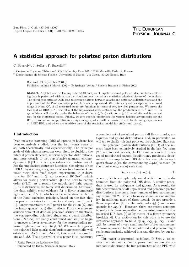
Fig. 1. The isovector structure functions 2xg(p−n)1 (x) and

F(p−n)2 (x). Data are taken from [13,15]

At this stage it is instructive to look at the availabledata shown in Fig. 1. We notice that these two functionshave very similar shapes and their difference is small andmainly positive, except perhaps for large x. In order to tryto identify the origin of this experimental fact, let us lookat the integrals of these functions divided by x. The firstone is twice the Bjorken sum rule [14], for which the bestworld estimate is IBj = 0.176± 0.005± 0.007 [15] and thesecond one is the Gottfried sum rule [12] whose value isIG = 0.235± 0.026 [13]. As a result using (9) one obtains,say for Q2 = 5GeV2,

∫ 1

0dx

[(d−(x) − u−(x)) + (d−(x) − u−(x))

]

= 0.175 ± 0.06. (10)

Now from the NMC result on the Gottfried sum rule onehas ∫ 1

0dx

[d(x) − u(x)

]= 0.16 ± 0.03. (11)

By comparing these two results we can assume, to a goodapproximation, the following relation for the helicity mi-nus distributions

d−(x) = u−(x). (12)

It follows from our procedure to construct antiquark dis-tributions from quark distributions described above (see(3)) that we automatically have for the helicity plus anti-quark distributions

d+(x) = u+(x), (13)

which makes (10) and (11) perfectly compatible. Indeed,as we will see below, (12) is rather well satisfied in thefinal determination of the distributions, after fitting thedata.

Let us now complete the description of our para-metrization. As stated above, the essential ingredient forquarks and antiquarks is a Fermi–Dirac distribution, asshown in (2), but we expect this piece to die out in thesmall x region, so we have to multiply it by a factorAXh

0qxb, where b > 0. In addition to A, a flavor and

helicity-independent normalization constant, we have in-troduced the factor Xh

0q which is needed to get a gooddescription of the data. It is not required by the simpleFermi–Dirac expression but, due to the ordering in (5),it will secure the correlation between the shape of a givendistribution and its first moment [7,16]. It is also in agree-ment with what has been found from data for the secondand third moments of the valence partons [17]. The smallx region is characterized by a rapid rise as x → 0 of thedistribution, which should be dominated by a universaldiffractive term, flavor and helicity independent, comingfrom the pomeron universality. Therefore we must add aterm of the form Axb/[exp(x/x)+1], where b < 0 and A isa normalization constant. So for the light quarks q = u, dof helicity h = ±, at the input energy scale Q2

0 = 4GeV2,we take

xqh(x,Q20) =

AXh0qx

b

exp[(x − Xh0q)/x] + 1

+Axb

exp(x/x) + 1,

(14)

and similarly for the light antiquarks

xqh(x,Q20) =

A(X−h0q )−1x2b

exp[(x+X−h0q )/x] + 1

+Axb

exp(x/x) + 1.

(15)

Here we take 2b for the power of x and not b as for quarks,an assumption we will try to justify later. For the strangequarks and antiquarks, s and s, given our poor knowledgeon both unpolarized and polarized distributions, we takethe particular choice

xs(x,Q20) = xs(x,Q2

0) =14

[xu(x,Q2

0) + xd(x,Q20)

],

(16)

and

x∆s(x,Q20) = x∆s(x,Q2

0)

=13

[x∆d(x,Q2

0) − x∆u(x,Q20)

]. (17)

This particular choice gives rise to a large negative ∆s(x,Q2

0) and we will come back to it below, in the discussion of


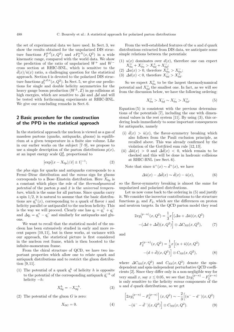
Fig. 2. The Fermi–Dirac functions for quarks F hq = Xh

0q/

(exp[(x − Xh0q)/x] + 1) at the input energy scale Q2

0 = 4GeV2,as a function of x

our results (see Sect. 4). The charm quarks c, both unpo-larized and polarized, are set to zero at Q2

0 = 4GeV2.Finally, concerning the gluon distribution, as indicatedabove, we use the Bose–Einstein expression

xG(x,Q20) =

AGxbG

exp(x/x) − 1, (18)

with a vanishing potential and the same temperature x.This choice is consistent with the idea that hadrons, in theDIS regime, are black body cavities for the color fields. It isalso reasonable to assume that for very small x, xG(x,Q2

0)has the same behavior as xq(x,Q2

0), so we will take bG =1+ b. Since the normalization constant AG is determinedfrom the momentum sum rule, our gluon distribution hasno free parameter. For the sake of completeness, we alsoneed to specify the polarized gluon distribution and wetake the particular choice

x∆G(x,Q20) = 0, (19)

consistent with (4). As usual, the valence contributionsare defined as qval = q − q, so A and A are determinedusing the normalization of uval(x) and dval(x), whose firstmoments are respectively 2 and 1.

To summarize, our parametrization involves a total ofeight free parameters

x, X+0u, X

−0u, X

−0d, X

+0d, b, b and A. (20)

In order to determine these parameters, we use a fittingprocedure on a selection of 233 data points at Q2 values,as close as possible to our input energy scale Q2

0 = 4GeV2,and the χ2 value we obtain is 322. For unpolarized DIS, wehave considered F p

2 (x,Q2) from NMC, BCDMS, E665 and

ZEUS, F d2 (x,Q

2) from NMC, E665 and xF νN3 (x,Q2) from

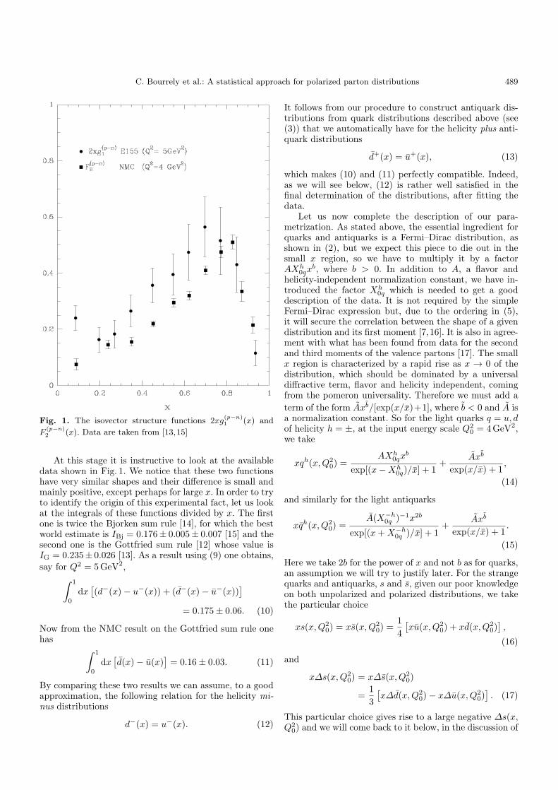
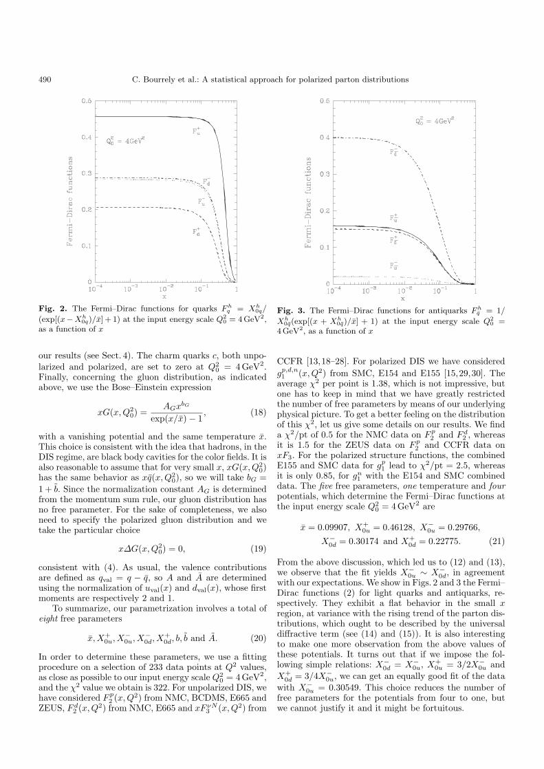
Fig. 3. The Fermi–Dirac functions for antiquarks F hq = 1/

Xh0q(exp[(x + Xh

0q)/x] + 1) at the input energy scale Q20 =

4GeV2, as a function of x

CCFR [13,18–28]. For polarized DIS we have consideredgp,d,n1 (x,Q2) from SMC, E154 and E155 [15,29,30]. Theaverage χ2 per point is 1.38, which is not impressive, butone has to keep in mind that we have greatly restrictedthe number of free parameters by means of our underlyingphysical picture. To get a better feeling on the distributionof this χ2, let us give some details on our results. We finda χ2/pt of 0.5 for the NMC data on F p

2 and F d2 , whereas

it is 1.5 for the ZEUS data on F p2 and CCFR data on

xF3. For the polarized structure functions, the combinedE155 and SMC data for gp

1 lead to χ2/pt = 2.5, whereasit is only 0.85, for gn

1 with the E154 and SMC combineddata. The five free parameters, one temperature and fourpotentials, which determine the Fermi–Dirac functions atthe input energy scale Q2

0 = 4GeV2 are

x = 0.09907, X+0u = 0.46128, X−

0u = 0.29766,

X−0d = 0.30174 and X+

0d = 0.22775. (21)

From the above discussion, which led us to (12) and (13),we observe that the fit yields X−

0u ∼ X−0d, in agreement

with our expectations. We show in Figs. 2 and 3 the Fermi–Dirac functions (2) for light quarks and antiquarks, re-spectively. They exhibit a flat behavior in the small xregion, at variance with the rising trend of the parton dis-tributions, which ought to be described by the universaldiffractive term (see (14) and (15)). It is also interestingto make one more observation from the above values ofthese potentials. It turns out that if we impose the fol-lowing simple relations: X−

0d = X−0u, X

+0u = 3/2X−

0u andX+

0d = 3/4X−0u, we can get an equally good fit of the data

with X−0u = 0.30549. This choice reduces the number of

free parameters for the potentials from four to one, butwe cannot justify it and it might be fortuitous.


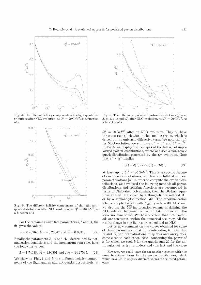
Fig. 4. The different helicity components of the light quark dis-tributions after NLO evolution, at Q2 = 20GeV2, as a functionof x

Fig. 5. The different helicity components of the light anti-quark distributions after NLO evolution, at Q2 = 20GeV2, asa function of x

For the remaining three free parameters b, b and A, thefit gives the values

b = 0.40962, b = −0.25347 and A = 0.08318. (22)

Finally the parameters A, A and AG, determined by nor-malization conditions and the momentum sum rule, havethe following values:

A = 1.74938, A = 1.90801 and AG = 14.27535. (23)

We show in Figs. 4 and 5 the different helicity compo-nents of the light quarks and antiquarks, respectively, at

Fig. 6. The different unpolarized parton distributions (f = u,d, u, d, s, c and G) after NLO evolution, at Q2 = 20GeV2, asa function of x

Q2 = 20GeV2, after an NLO evolution. They all havethe same rising behavior in the small x region, which isdriven by the universal diffractive term. We note that af-ter NLO evolution, we still have u− ∼ d− and u+ ∼ d+.In Fig. 6, we display the x-shapes of the full set of unpo-larized parton distributions, where one sees a non-zero cquark distribution generated by the Q2 evolution. Notethat u− ∼ d− implies

u(x) − d(x) ∼ ∆u(x) − ∆d(x) (24)

at least up to Q2 ∼ 20GeV2. This is a specific featureof our quark distributions, which is not fulfilled in mostparametrizations [3]. In order to compute the evolved dis-tributions, we have used the following method: all partondistributions and splitting functions are decomposed interms of Chebyshev polynomials, then the DGLAP equa-tions at NLO are solved by a Runge–Kutta method [31]or by a semianalytic method [32]. The renormalizationscheme adopted is MS with ΛMS[nf = 3] = 300MeV andwe also use the MS factorization scheme in defining theNLO relation between the parton distributions and thestructure functions1. We have checked that both meth-ods are consistent, within the numerical accuracy. All theresults shown in the figures are calculated at NLO.

Let us now comment on the values obtained for someof these parameters. First, it is interesting to note thatA and A, the normalizations of quarks and antiquarks,come close to each other. Next, concerning the power ofx for which we took b for the quarks and 2b for the an-tiquarks, let us try to understand this fact and the value

1 However, we could have chosen another scheme with thesame functional forms for the parton distributions, whichwould have led to slightly different values of the fitted param-eters


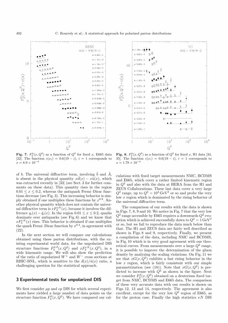
Fig. 7. F p2 (x, Q2) as a function of Q2 for fixed x, E665 data

[22]. The function c(xi) = 0.6(19 − i), i = 1 corresponds tox = 8.9 × 10−4

of b. The universal diffractive term, involving b and A,is absent in the physical quantity xd(x) − xu(x), whichwas extracted recently in [33] (see Sect. 3 for further com-ments on these data). This quantity rises in the region0.01 ≤ x ≤ 0.2, whereas the antiquark Fermi–Dirac func-tions decrease (see Fig. 3). This increasing behavior is sim-ply obtained if one multiplies these functions by x0.8. An-other physical quantity which does not contain the univer-sal diffractive term is xF νN

3 (x), because it involves the dif-ference qi(x)− qi(x). In the region 0.01 ≤ x ≤ 0.2, quarksdominate over antiquarks (see Fig. 6) and we know thatxF νN

3 (x) rises. This behavior is obtained if one multipliesthe quark Fermi–Dirac function by x0.4, in agreement with(22).

In the next section we will compare our calculationsobtained using these parton distributions, with the ex-isting experimental world data, for the unpolarized DISstructure functions F p,d

2 (x,Q2) and xF νN3 (x,Q2), in a

wide kinematic range. We will also show the predictionof the ratio of unpolarized W+ and W− cross sections atRHIC-BNL, which is sensitive to the d(x)/u(x) ratio, achallenging question for the statistical approach.

3 Experimental tests for unpolarized DIS

We first consider µp and ep DIS for which several experi-ments have yielded a large number of data points on thestructure function F p

2 (x,Q2). We have compared our cal-

Fig. 8. F p2 (x, Q2) as a function of Q2 for fixed x, H1 data [34,

35]. The function c(xi) = 0.6(19 − i), i = 1 corresponds tox = 1.78 × 10−4

culations with fixed target measurements NMC, BCDMSand E665, which cover a rather limited kinematic regionin Q2 and also with the data at HERA from the H1 andZEUS Collaborations. These last data cover a very largeQ2 range, up to Q2 = 104 GeV2 or so and probe the verylow x region which is dominated by the rising behavior ofthe universal diffractive term.

The comparison of our results with the data is shownin Figs. 7, 8, 9 and 10. We notice in Fig. 7 that the very lowQ2 range accessible by E665 requires a downwards Q2 evo-lution which is achieved successfully down to Q2 = 1GeV2

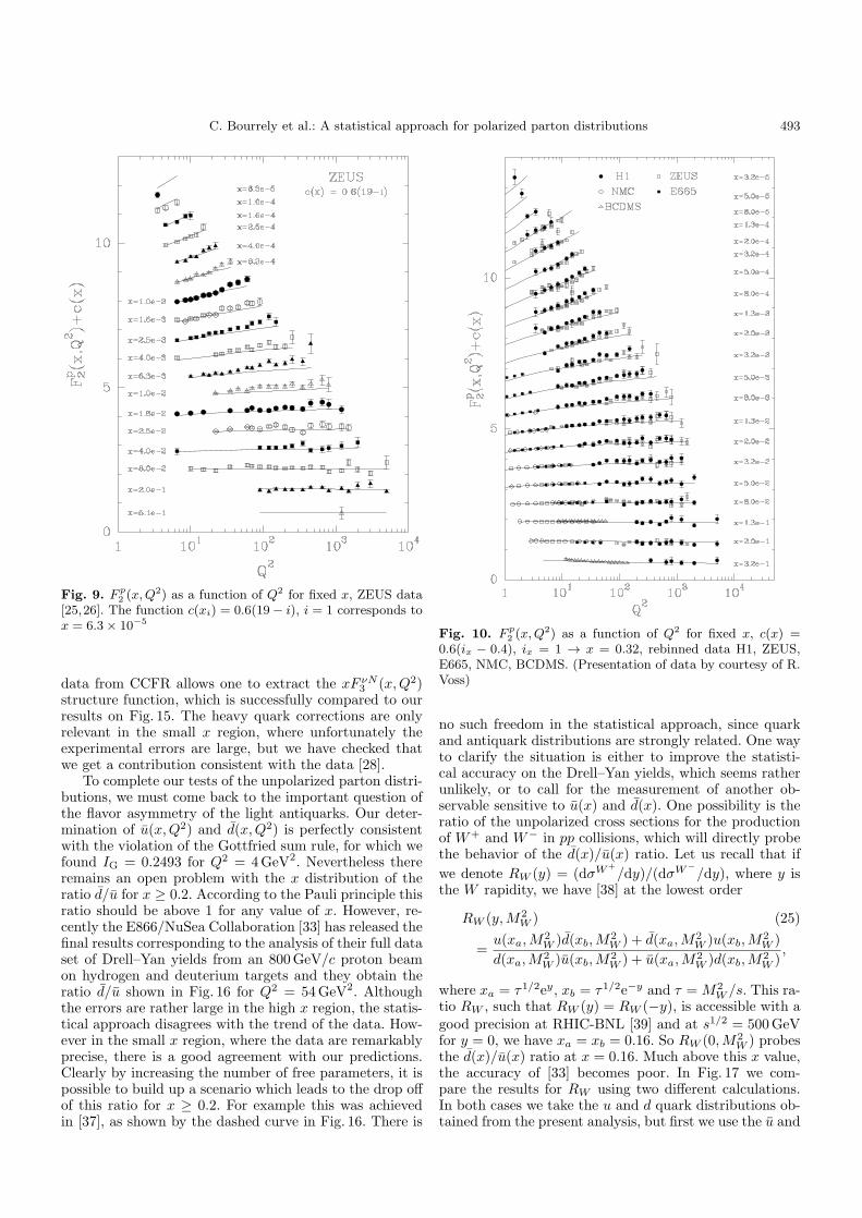
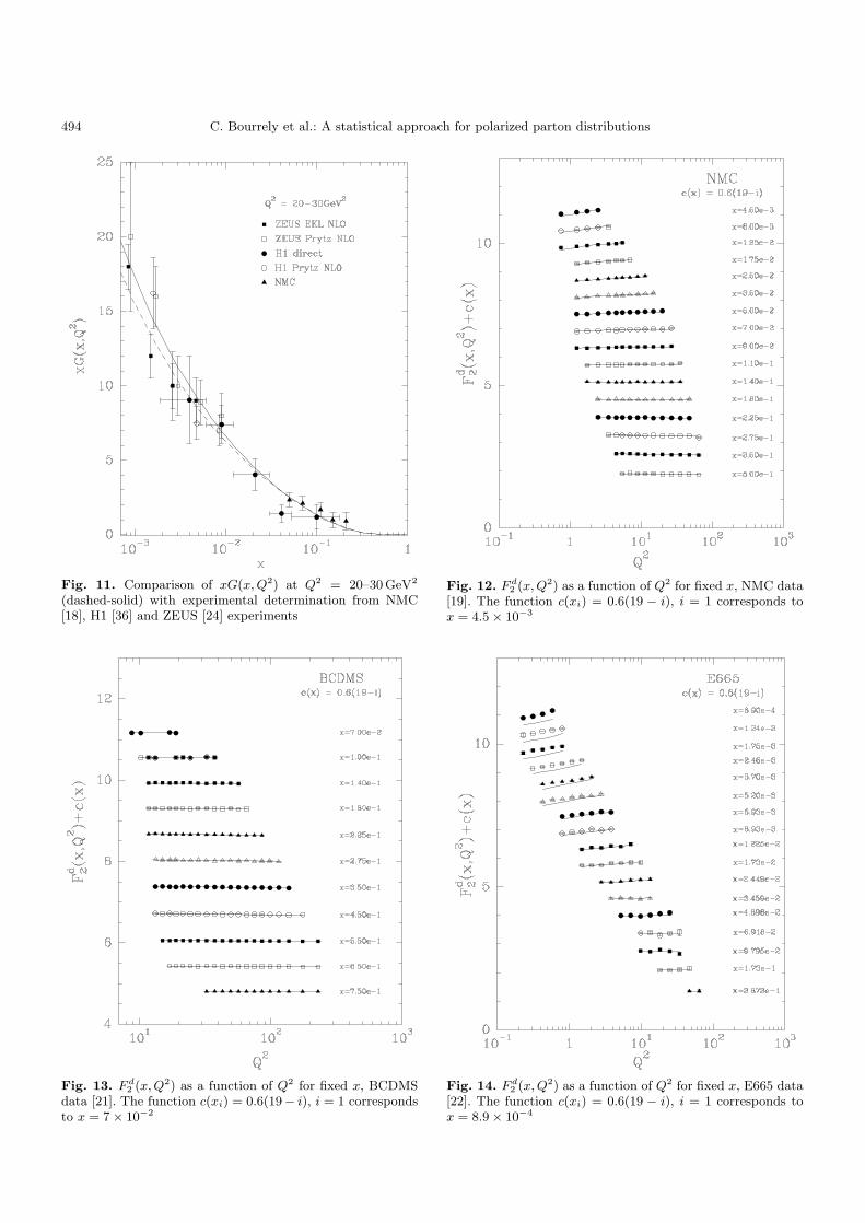
or so, but we fail to reproduce the data much below thanthat. The H1 and ZEUS data are fairly well described asshown in Figs. 8 and 9, respectively. Finally, we presenta compilation of the data, including NMC and BCDMS,in Fig. 10 which is in very good agreement with our theo-retical curves. From measurements over a large Q2 range,it is possible to improve the determination of the gluondensity by analyzing the scaling violations. On Fig. 11 wesee that xG(x,Q2) exhibits a fast rising behavior in thelow x region, which is fairly consistent with our simpleparametrization (see (18)). Note that xG(x,Q2) is pre-dicted to increase with Q2 as shown in the figure. Nextwe consider F d

2 (x,Q2) obtained on a deuterium fixed tar-

get from NMC, BCDMS and E665 data. The comparisonof these very accurate data with our results is shown onFigs. 12, 13 and 14, respectively. The agreement is alsoexcellent, except for the very low Q2 region of E665, asfor the proton case. Finally the high statistics νN DIS


Fig. 9. F p2 (x, Q2) as a function of Q2 for fixed x, ZEUS data

[25,26]. The function c(xi) = 0.6(19 − i), i = 1 corresponds tox = 6.3 × 10−5

data from CCFR allows one to extract the xF νN3 (x,Q2)

structure function, which is successfully compared to ourresults on Fig. 15. The heavy quark corrections are onlyrelevant in the small x region, where unfortunately theexperimental errors are large, but we have checked thatwe get a contribution consistent with the data [28].

To complete our tests of the unpolarized parton distri-butions, we must come back to the important question ofthe flavor asymmetry of the light antiquarks. Our deter-mination of u(x,Q2) and d(x,Q2) is perfectly consistentwith the violation of the Gottfried sum rule, for which wefound IG = 0.2493 for Q2 = 4GeV2. Nevertheless thereremains an open problem with the x distribution of theratio d/u for x ≥ 0.2. According to the Pauli principle thisratio should be above 1 for any value of x. However, re-cently the E866/NuSea Collaboration [33] has released thefinal results corresponding to the analysis of their full dataset of Drell–Yan yields from an 800GeV/c proton beamon hydrogen and deuterium targets and they obtain theratio d/u shown in Fig. 16 for Q2 = 54GeV2. Althoughthe errors are rather large in the high x region, the statis-tical approach disagrees with the trend of the data. How-ever in the small x region, where the data are remarkablyprecise, there is a good agreement with our predictions.Clearly by increasing the number of free parameters, it ispossible to build up a scenario which leads to the drop offof this ratio for x ≥ 0.2. For example this was achievedin [37], as shown by the dashed curve in Fig. 16. There is

Fig. 10. F p2 (x, Q2) as a function of Q2 for fixed x, c(x) =

0.6(ix − 0.4), ix = 1 → x = 0.32, rebinned data H1, ZEUS,E665, NMC, BCDMS. (Presentation of data by courtesy of R.Voss)

no such freedom in the statistical approach, since quarkand antiquark distributions are strongly related. One wayto clarify the situation is either to improve the statisti-cal accuracy on the Drell–Yan yields, which seems ratherunlikely, or to call for the measurement of another ob-servable sensitive to u(x) and d(x). One possibility is theratio of the unpolarized cross sections for the productionof W+ and W− in pp collisions, which will directly probethe behavior of the d(x)/u(x) ratio. Let us recall that ifwe denote RW (y) = (dσW+

/dy)/(dσW −/dy), where y is

the W rapidity, we have [38] at the lowest order

RW (y,M2W ) (25)

=u(xa,M

2W )d(xb,M

2W ) + d(xa,M

2W )u(xb,M

2W )

d(xa,M2W )u(xb,M2

W ) + u(xa,M2W )d(xb,M2

W ),

where xa = τ1/2ey, xb = τ1/2e−y and τ = M2W /s. This ra-

tio RW , such that RW (y) = RW (−y), is accessible with agood precision at RHIC-BNL [39] and at s1/2 = 500GeVfor y = 0, we have xa = xb = 0.16. So RW (0,M2

W ) probesthe d(x)/u(x) ratio at x = 0.16. Much above this x value,the accuracy of [33] becomes poor. In Fig. 17 we com-pare the results for RW using two different calculations.In both cases we take the u and d quark distributions ob-tained from the present analysis, but first we use the u and


Fig. 11. Comparison of xG(x, Q2) at Q2 = 20–30GeV2

(dashed-solid) with experimental determination from NMC[18], H1 [36] and ZEUS [24] experiments

Fig. 12. F d2 (x, Q2) as a function of Q2 for fixed x, NMC data


Fig. 13. F d2 (x, Q2) as a function of Q2 for fixed x, BCDMS

data [21]. The function c(xi) = 0.6(19− i), i = 1 correspondsto x = 7 × 10−2

Fig. 14. F d2 (x, Q2) as a function of Q2 for fixed x, E665 data



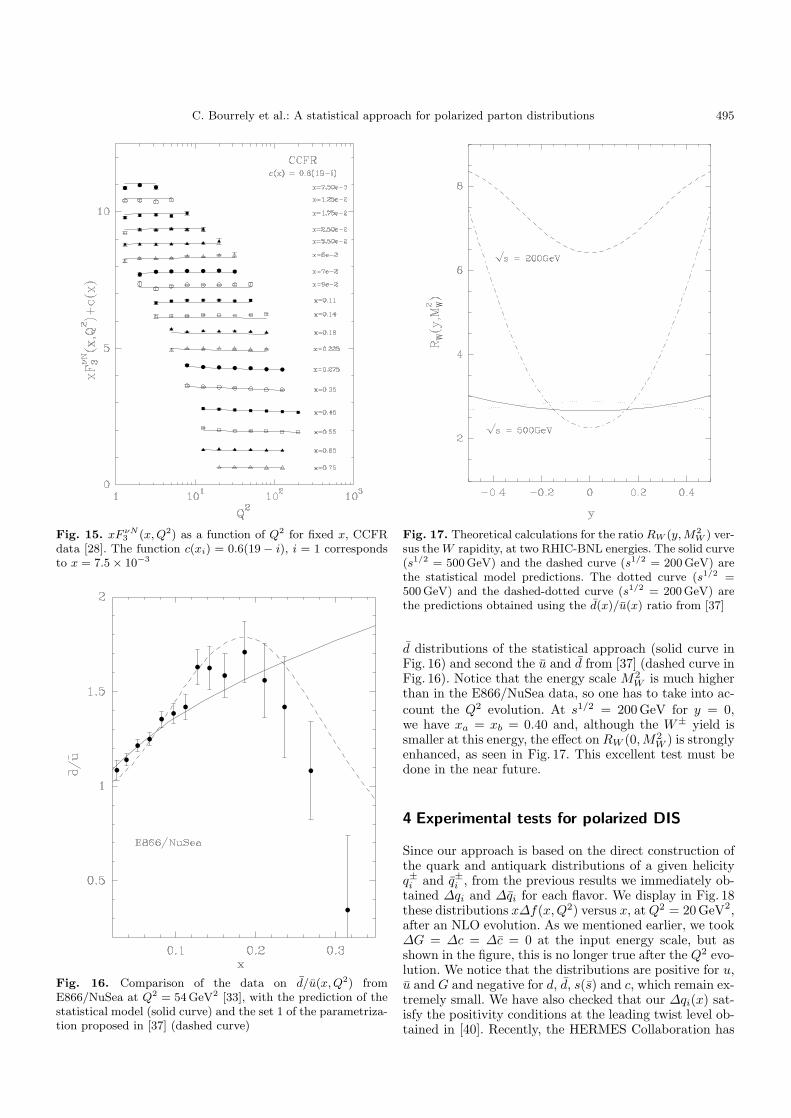
Fig. 15. xF νN3 (x, Q2) as a function of Q2 for fixed x, CCFR

data [28]. The function c(xi) = 0.6(19 − i), i = 1 correspondsto x = 7.5 × 10−3

Fig. 16. Comparison of the data on d/u(x, Q2) fromE866/NuSea at Q2 = 54GeV2 [33], with the prediction of thestatistical model (solid curve) and the set 1 of the parametriza-tion proposed in [37] (dashed curve)

Fig. 17. Theoretical calculations for the ratio RW (y, M2W ) ver-

sus the W rapidity, at two RHIC-BNL energies. The solid curve(s1/2 = 500GeV) and the dashed curve (s1/2 = 200GeV) arethe statistical model predictions. The dotted curve (s1/2 =500GeV) and the dashed-dotted curve (s1/2 = 200GeV) arethe predictions obtained using the d(x)/u(x) ratio from [37]

d distributions of the statistical approach (solid curve inFig. 16) and second the u and d from [37] (dashed curve inFig. 16). Notice that the energy scale M2

W is much higherthan in the E866/NuSea data, so one has to take into ac-count the Q2 evolution. At s1/2 = 200GeV for y = 0,we have xa = xb = 0.40 and, although the W± yield issmaller at this energy, the effect on RW (0,M2

W ) is stronglyenhanced, as seen in Fig. 17. This excellent test must bedone in the near future.

4 Experimental tests for polarized DIS

Since our approach is based on the direct construction ofthe quark and antiquark distributions of a given helicityq±i and q±

i , from the previous results we immediately ob-tained ∆qi and ∆qi for each flavor. We display in Fig. 18these distributions x∆f(x,Q2) versus x, atQ2 = 20GeV2,after an NLO evolution. As we mentioned earlier, we took∆G = ∆c = ∆c = 0 at the input energy scale, but asshown in the figure, this is no longer true after the Q2 evo-lution. We notice that the distributions are positive for u,u and G and negative for d, d, s(s) and c, which remain ex-tremely small. We have also checked that our ∆qi(x) sat-isfy the positivity conditions at the leading twist level ob-tained in [40]. Recently, the HERMES Collaboration has


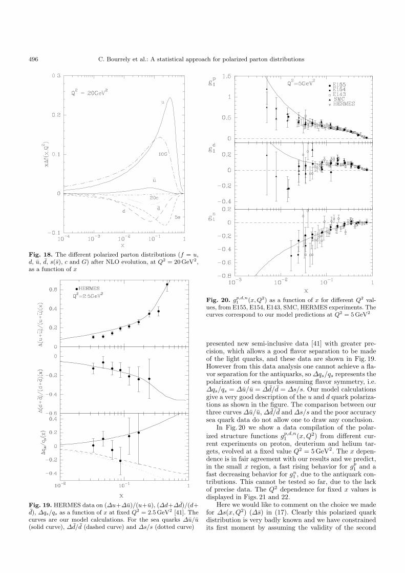
Fig. 18. The different polarized parton distributions (f = u,d, u, d, s(s), c and G) after NLO evolution, at Q2 = 20GeV2,as a function of x

Fig. 19. HERMES data on (∆u+∆u)/(u+u), (∆d+∆d)/(d+d), ∆qs/qs as a function of x at fixed Q2 = 2.5GeV2 [41]. Thecurves are our model calculations. For the sea quarks ∆u/u(solid curve), ∆d/d (dashed curve) and ∆s/s (dotted curve)

Fig. 20. gp,d,n1 (x, Q2) as a function of x for different Q2 val-

ues, from E155, E154, E143, SMC, HERMES experiments. Thecurves correspond to our model predictions at Q2 = 5GeV2

presented new semi-inclusive data [41] with greater pre-cision, which allows a good flavor separation to be madeof the light quarks, and these data are shown in Fig. 19.However from this data analysis one cannot achieve a fla-vor separation for the antiquarks, so∆qs/qs represents thepolarization of sea quarks assuming flavor symmetry, i.e.∆qs/qs = ∆u/u = ∆d/d = ∆s/s. Our model calculationsgive a very good description of the u and d quark polariza-tions as shown in the figure. The comparison between ourthree curves ∆u/u, ∆d/d and ∆s/s and the poor accuracysea quark data do not allow one to draw any conclusion.

In Fig. 20 we show a data compilation of the polar-ized structure functions gp,d,n

1 (x,Q2) from different cur-rent experiments on proton, deuterium and helium tar-gets, evolved at a fixed value Q2 = 5GeV2. The x depen-dence is in fair agreement with our results and we predict,in the small x region, a fast rising behavior for gp

1 and afast decreasing behavior for gn

1 , due to the antiquark con-tributions. This cannot be tested so far, due to the lackof precise data. The Q2 dependence for fixed x values isdisplayed in Figs. 21 and 22.

Here we would like to comment on the choice we madefor ∆s(x,Q2) (∆s) in (17). Clearly this polarized quarkdistribution is very badly known and we have constrainedits first moment by assuming the validity of the second


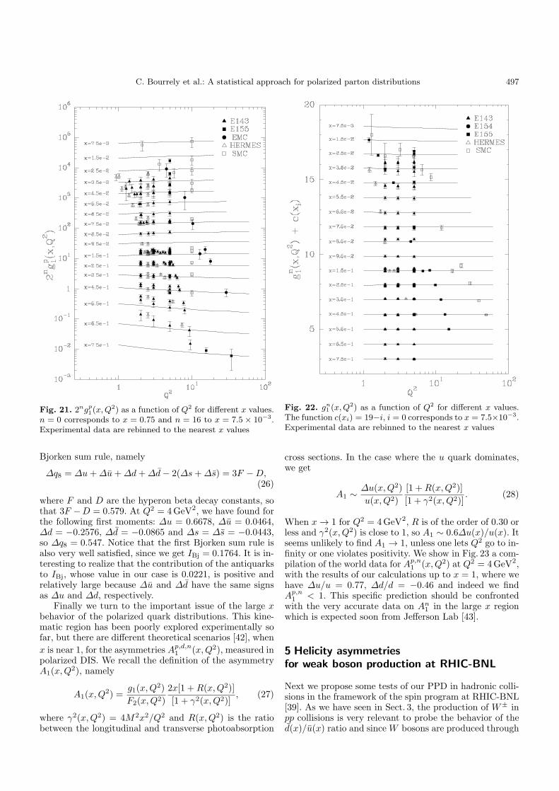
Fig. 21. 2ngp1(x, Q2) as a function of Q2 for different x values.

n = 0 corresponds to x = 0.75 and n = 16 to x = 7.5 × 10−3.Experimental data are rebinned to the nearest x values

Bjorken sum rule, namely

∆q8 = ∆u+∆u+∆d+∆d − 2(∆s+∆s) = 3F − D,(26)

where F and D are the hyperon beta decay constants, sothat 3F −D = 0.579. At Q2 = 4GeV2, we have found forthe following first moments: ∆u = 0.6678, ∆u = 0.0464,∆d = −0.2576, ∆d = −0.0865 and ∆s = ∆s = −0.0443,so ∆q8 = 0.547. Notice that the first Bjorken sum rule isalso very well satisfied, since we get IBj = 0.1764. It is in-teresting to realize that the contribution of the antiquarksto IBj, whose value in our case is 0.0221, is positive andrelatively large because ∆u and ∆d have the same signsas ∆u and ∆d, respectively.

Finally we turn to the important issue of the large xbehavior of the polarized quark distributions. This kine-matic region has been poorly explored experimentally sofar, but there are different theoretical scenarios [42], whenx is near 1, for the asymmetries Ap,d,n

1 (x,Q2), measured inpolarized DIS. We recall the definition of the asymmetryA1(x,Q2), namely

A1(x,Q2) =g1(x,Q2)F2(x,Q2)

2x[1 +R(x,Q2)][1 + γ2(x,Q2)]

, (27)

where γ2(x,Q2) = 4M2x2/Q2 and R(x,Q2) is the ratiobetween the longitudinal and transverse photoabsorption

Fig. 22. gn1 (x, Q2) as a function of Q2 for different x values.

The function c(xi) = 19−i, i = 0 corresponds to x = 7.5×10−3.Experimental data are rebinned to the nearest x values

cross sections. In the case where the u quark dominates,we get

A1 ∼ ∆u(x,Q2)u(x,Q2)

[1 +R(x,Q2)][1 + γ2(x,Q2)]

. (28)

When x → 1 for Q2 = 4GeV2, R is of the order of 0.30 orless and γ2(x,Q2) is close to 1, so A1 ∼ 0.6∆u(x)/u(x). Itseems unlikely to find A1 → 1, unless one lets Q2 go to in-finity or one violates positivity. We show in Fig. 23 a com-pilation of the world data for Ap,n

1 (x,Q2) at Q2 = 4GeV2,with the results of our calculations up to x = 1, where wehave ∆u/u = 0.77, ∆d/d = −0.46 and indeed we findAp,n

1 < 1. This specific prediction should be confrontedwith the very accurate data on An

1 in the large x regionwhich is expected soon from Jefferson Lab [43].

5 Helicity asymmetriesfor weak boson production at RHIC-BNL

Next we propose some tests of our PPD in hadronic colli-sions in the framework of the spin program at RHIC-BNL[39]. As we have seen in Sect. 3, the production of W± inpp collisions is very relevant to probe the behavior of thed(x)/u(x) ratio and since W bosons are produced through


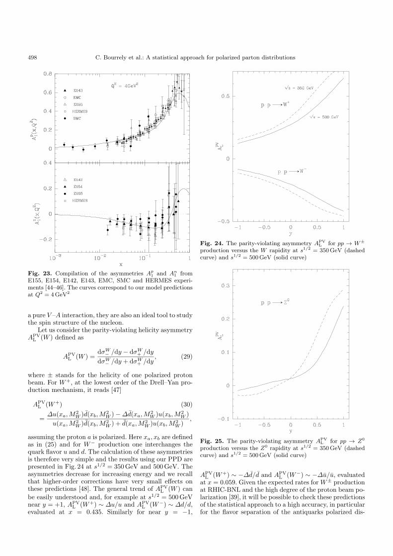
Fig. 23. Compilation of the asymmetries Ap1 and An

1 fromE155, E154, E142, E143, EMC, SMC and HERMES experi-ments [44–46]. The curves correspond to our model predictionsat Q2 = 4GeV2

a pure V –A interaction, they are also an ideal tool to studythe spin structure of the nucleon.

Let us consider the parity-violating helicity asymmetryAPV

L (W ) defined as

APVL (W ) =

dσW− /dy − dσW

+ /dydσW− /dy + dσW

+ /dy, (29)

where ± stands for the helicity of one polarized protonbeam. For W+, at the lowest order of the Drell–Yan pro-duction mechanism, it reads [47]

APVL (W+) (30)

=∆u(xa,M

2W )d(xb,M

2W ) − ∆d(xa,M

2W )u(xb,M

2W )

u(xa,M2W )d(xb,M2

W ) + d(xa,M2W )u(xb,M2

W ),

assuming the proton a is polarized. Here xa, xb are definedas in (25) and for W− production one interchanges thequark flavor u and d. The calculation of these asymmetriesis therefore very simple and the results using our PPD arepresented in Fig. 24 at s1/2 = 350GeV and 500GeV. Theasymmetries decrease for increasing energy and we recallthat higher-order corrections have very small effects onthese predictions [48]. The general trend of APV

L (W ) canbe easily understood and, for example at s1/2 = 500GeVnear y = +1, APV

L (W+) ∼ ∆u/u and APVL (W−) ∼ ∆d/d,

evaluated at x = 0.435. Similarly for near y = −1,

Fig. 24. The parity-violating asymmetry APVL for pp → W ±

production versus the W rapidity at s1/2 = 350GeV (dashedcurve) and s1/2 = 500GeV (solid curve)

Fig. 25. The parity-violating asymmetry APVL for pp → Z0

production versus the Z0 rapidity at s1/2 = 350GeV (dashedcurve) and s1/2 = 500GeV (solid curve)

APVL (W+) ∼ −∆d/d and APV

L (W−) ∼ −∆u/u, evaluatedat x = 0.059. Given the expected rates for W± productionat RHIC-BNL and the high degree of the proton beam po-larization [39], it will be possible to check these predictionsof the statistical approach to a high accuracy, in particularfor the flavor separation of the antiquarks polarized dis-


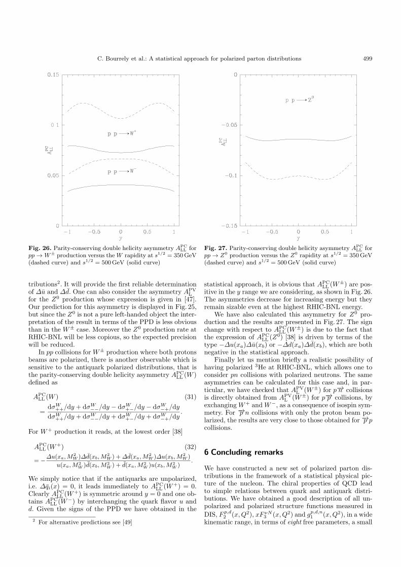
Fig. 26. Parity-conserving double helicity asymmetry APCLL for

pp → W ± production versus the W rapidity at s1/2 = 350GeV(dashed curve) and s1/2 = 500GeV (solid curve)

tributions2. It will provide the first reliable determinationof ∆u and ∆d. One can also consider the asymmetry APV

Lfor the Z0 production whose expression is given in [47].Our prediction for this asymmetry is displayed in Fig. 25,but since the Z0 is not a pure left-handed object the inter-pretation of the result in terms of the PPD is less obviousthan in the W± case. Moreover the Z0 production rate atRHIC-BNL will be less copious, so the expected precisionwill be reduced.

In pp collisions for W± production where both protonsbeams are polarized, there is another observable which issensitive to the antiquark polarized distributions, that isthe parity-conserving double helicity asymmetry APC

LL (W )defined as

APCLL (W ) (31)

=dσW

++/dy + dσW−−/dy − dσW

+−/dy − dσW−+/dy

dσW++/dy + dσW−−/dy + dσW

+−/dy + dσW−+/dy.

For W+ production it reads, at the lowest order [38]

APCLL (W

+) (32)

= −∆u(xa, M2W )∆d(xb, M

2W ) + ∆d(xa, M2

W )∆u(xb, M2W )

u(xa, M2W )d(xb, M2

W ) + d(xa, M2W )u(xb, M2

W ).

We simply notice that if the antiquarks are unpolarized,i.e. ∆qi(x) = 0, it leads immediately to APC

LL (W+) = 0.

Clearly APCLL (W

+) is symmetric around y = 0 and one ob-tains APC

LL (W−) by interchanging the quark flavor u and

d. Given the signs of the PPD we have obtained in the

2 For alternative predictions see [49]

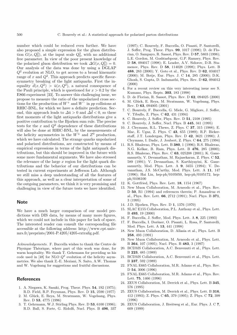
Fig. 27. Parity-conserving double helicity asymmetry APCLL for

pp → Z0 production versus the Z0 rapidity at s1/2 = 350GeV(dashed curve) and s1/2 = 500GeV (solid curve)

statistical approach, it is obvious that APCLL (W

±) are pos-itive in the y range we are considering, as shown in Fig. 26.The asymmetries decrease for increasing energy but theyremain sizable even at the highest RHIC-BNL energy.

We have also calculated this asymmetry for Z0 pro-duction and the results are presented in Fig. 27. The signchange with respect to APC

LL (W±) is due to the fact that

the expression of APCLL (Z

0) [38] is driven by terms of thetype −∆u(xa)∆u(xb) or −∆d(xa)∆d(xb), which are bothnegative in the statistical approach.

Finally let us mention briefly a realistic possibility ofhaving polarized 3He at RHIC-BNL, which allows one toconsider pn collisions with polarized neutrons. The sameasymmetries can be calculated for this case and, in par-ticular, we have checked that APV

L (W±) for p−→n collisionsis directly obtained from APV

L (W±) for p−→p collisions, byexchanging W+ and W−, as a consequence of isospin sym-metry. For −→p n collisions with only the proton beam po-larized, the results are very close to those obtained for −→p pcollisions.

6 Concluding remarks

We have constructed a new set of polarized parton dis-tributions in the framework of a statistical physical pic-ture of the nucleon. The chiral properties of QCD leadto simple relations between quark and antiquark distri-butions. We have obtained a good description of all un-polarized and polarized structure functions measured inDIS, F p,d

2 (x,Q2), xF νN3 (x,Q2) and gp,d,n

1 (x,Q2), in a widekinematic range, in terms of eight free parameters, a small


number which could be reduced even further. We havealso proposed a simple expression for the gluon distribu-tion G(x,Q2

0), at the input scale Q20, with no additional

free parameter. In view of the poor present knowledge ofthe polarized gluon distribution we took ∆G(x,Q2

0) = 0.Our analysis of the data was done by using a DGLAPQ2 evolution at NLO, to get access to a broad kinematicrange of x and Q2. This approach predicts specific flavor-symmetry breaking of the light antiquarks. First the in-equality d(x,Q2) > u(x,Q2), a natural consequence ofthe Pauli principle, which is questioned for x > 0.2 by theE866 experiment [33]. To answer this challenging issue, wepropose to measure the ratio of the unpolarized cross sec-tions for the production of W+ and W− in pp collisions atRHIC-BNL, for which we have a definite prediction. Sec-ond, this approach leads to ∆u > 0 and ∆d < 0, so thesefirst moments of the light antiquarks distributions give apositive contribution to the Bjorken sum rule. The precisetests for the x and Q2 dependence of these distributionswill also be done at RHIC-BNL, by the measurements ofthe helicity asymmetries in the W± and Z0 production,which we have calculated. The strange quarks unpolarizedand polarized distributions, are constructed by means ofempirical expressions in terms of the light antiquark dis-tributions, but this should be improved in the future withsome more fundamental arguments. We have also stressedthe relevance of the large x region for the light quark dis-tributions and the behavior of our distributions can betested in current experiments at Jefferson Lab. Althoughwe still miss a deep understanding of all the features ofthis approach, as well as a clear interpretation of some ofthe outgoing parameters, we think it is very promising andchallenging in view of the future tests we have identified.

Note

We have a much larger comparison of our model pre-dictions with DIS data, by means of many more figures,which we could not include in this paper for lack of space.The interested reader can consult the corresponding fileaccessible at the following address: http://www.cpt.univ-mrs.fr/preprints/2001-P.4205/4205-extrafig.pdf.

Acknowledgements. F. Buccella wishes to thank the Centre dePhysique Theorique, where part of this work was done, forwarm hospitality. We thank T. Gehrmann for providing us hiscode used in [48] for NLO Q2 evolution of the helicity asym-metries. We also thank Z.-E. Meziani, N. Saito, A.W. Thomasand W. Vogelsang for suggestions and fruitful discussions.

References

1. A. Niegawa, K. Sasaki, Prog. Theor. Phys. 54, 192 (1975);R.D. Field, R.P. Feynman, Phys. Rev. D 15, 2590 (1977)

2. M. Gluck, E. Reya, M. Stratmann, W. Vogelsang, Phys.Rev. D 53, 4775 (1996)

3. T. Gehrmann, W.J. Stirling Phys. Rev. D 53, 6100 (1996);R.D. Ball, S. Forte, G. Ridolfi, Nucl. Phys. B 496, 337

(1997); C. Bourrely, F. Buccella, O. Pisanti, P. Santorelli,J. Soffer, Prog. Theor. Phys. 99, 1017 (1998); D. de Flo-rian, O. Sampayo, R. Sassot, Phys. Rev. D 57, 5803 (1998);L.E. Gordon, M. Goshtasbpour, G.P. Ramsey, Phys. Rev.D 58, 094017 (1998); E. Leader, A.V. Sidorov, D.B. Sta-menov, Phys. Rev. D 58, 114028 (1998); Phys. Lett. B488, 283 (2000); Y. Goto et al., Phys. Rev. D 62, 034017(2000); M. Botje, Eur. Phys. J. C 14, 285 (2000); D.K.Ghosh, S. Gupta, D. Indumathi, Phys. Rev. D 62, 094012(2000)

4. For a recent review on this very interesting issue see S.Kumano, Phys. Repts. 303, 183 (1998)

5. D. de Florian, R. Sassot, Phys. Rev. D 62, 094025 (2000)6. M. Gluck, E. Reya, M. Stratmann, W. Vogelsang, Phys.

Rev. D 63, 094005 (2001)7. C. Bourrely, F. Buccella, G. Miele, G. Migliore, J. Soffer,

V. Tibullo, Z. Phys. C 62, 431 (1994)8. C. Bourrely, J. Soffer, Phys. Rev. D 51, 2108 (1995)9. C. Bourrely, J. Soffer, Nucl. Phys. B 445, 341 (1995)10. J. Cleymans, R.L. Thews, Z. Phys. C 37, 315 (1988); E.

Mac, E. Ugaz, Z. Phys. C 43, 655 (1989); R.P. Bicker-staff, J.T. Londergan, Phys. Rev. D 42, 3621 (1990); J.Cleymans, I. Dadic, J. Joubert, Z. Phys. C 64, 275 (1994)

11. R.S. Bhalerao, Phys. Lett. B 380, 1 (1996); R.S. Bhalerao,N.G. Kelkar, B. Ram, Phys. Lett. B 476, 285 (2000);R.S. Bhalerao, Phys. Rev. C 63, 025208 (2001); K. Gane-samurtly, V. Devanathan, M. Rajasekaran, Z. Phys. C 52,589 (1991); V. Devanathan, S. Karthiyayini, K. Gane-samurtly, Mod. Phys. Lett. A 9, 3455 (1994); V. De-vanathan, J.S. McCarthy, Mod. Phys. Lett. A 11, 147(1996); Hai Lin, hep-ph/0105050, hep-ph/0105172, hep-ph/0106100

12. K. Gottfried, Phys. Rev. Lett. 18, 1154 (1967)13. New Muon Collaboration, M. Arneodo et al., Phys. Rev.

D 50, R1 (1994) and references therein; P. Amaudruz etal., Phys. Rev. Lett. 66, 2712 (1991); Nucl. Phys. B 371,3 (1995)

14. J.D. Bjorken, Phys. Rev. D 1, 1376 (1970)15. SLAC E155 Collaboration, P.L. Anthony et al., Phys. Lett.

B 493, 19 (2000)16. F. Buccella, J. Soffer, Mod. Phys. Lett. A 8, 225 (1993)17. F. Buccella, I. Dorsner, O. Pisanti, L. Rosa, P. Santorelli,

Mod. Phys. Lett. A 13, 441 (1998)18. New Muon Collaboration, D. Allasia et al., Phys. Lett. B

258, 493 (1991)19. New Muon Collaboration, M. Arneodo et al., Phys. Lett.

B 364, 107 (1995); Nucl. Phys. B 483, 3 (1997)20. BCDMS Collaboration, A.C. Benvenuti et al., Phys. Lett.

B 223, 485 (1989)21. BCDMS Collaboration, A.C. Benvenuti et al., Phys. Lett.

B 237, 592 (1989)22. FNAL E665 Collaboration, M.R. Adams et al., Phys. Rev.

D 54, 3006 (1996)23. FNAL E665 Collaboration, M.R. Adams et al., Phys. Rev.

Lett. 75, 1466 (1996)24. ZEUS Collaboration, M. Derrick et al., Phys. Lett. B 345,

576 (1995)25. ZEUS Collaboration, M. Derrick et al., Phys. Lett. B 316,

412 (1993); Z. Phys. C 65, 379 (1995); Z. Phys. C 72, 399(1996)

26. ZEUS Collaboration, J. Breitweg et al., Eur. Phys. J. C 7,609 (1999)


27. ZEUS Collaboration, XXX International Conference HighEnergy Physics, Osaka (Japan) July 2000, abstract 1049;J. Breitweg et al., Eur. Phys. J. C 11, 427 (1999)

28. CCFR Collaboration, P.Z. Quintas et al., Phys. Rev. Lett.71, 1307 (1993); W.C. Leung et al., Phys. Lett. B 317,655 (1993); W.G. Seligman et al., Phys. Rev. Lett. 79,1213 (1997); J.H. Kim et al., Phys. Rev. Lett. 81, 3595(1998); U.K. Yang et al., Phys. Rev. Lett. 86, 2741 (2001)

29. SMC Collaboration, B. Adeva et al., Phys. Rev. D 58,112001 (1998); Phys. Rev. D 60, 072004 (1999)

30. SLAC E154 Collaboration, K. Abe et al., Phys. Lett. B405, 180 (1997); Phys. Rev. Lett. 79, 26 (1997)

31. J. Kwiecinski, D. Strozik-Kotloz, Z. Phys. C 48, 315 (1990)32. P. Santorelli, E. Scrimieri, Phys. Lett. B 459, 599 (1999)33. FNAL Nusea Collaboration, E.A. Hawker et al., Phys.

Rev. Lett. 80, 3715 (1998); J.C. Peng et al., Phys. Rev.D 58, 092004 (1998); R.S. Towell et al., Phys. Rev. D 64,052002 (2001)

34. H1 Collaboration, S. Aid et al., Nucl. Phys. B 470, 3(1996); T. Ahmed et al., Nucl. Phys. B 439, 471 (1995);C. Adloff et al., Nucl. Phys. B 497, 3 (1996)

35. H1 Collaboration, C. Adloff et al., Eur. Phys. J. C 13, 609(2000)

36. H1 Collaboration, S. Aid et al., Nucl. Phys. B 449, 3 (1995)

37. A. Daleo, C.A. Garcıa Canal, G.A. Navarro, R. Sassot,hep-ph/0106156

38. C. Bourrely, J. Soffer, Nucl. Phys. B 423, 329 (1994)39. G. Bunce, N. Saito, J. Soffer, W. Vogelsang, Ann. Rev.

Nucl. Part. Scie. 50, 525 (2000)40. J. Soffer, O. Teryaev, Phys. Lett. B 490, 106 (2000)41. HERMES Collaboration, K. Ackerstaff et al., Phys. Lett.

B 404, 383 (1997); Phys. Lett. B 464, 123 (1999); A.Airapetian et al., Phys. Lett. B 442, 484 (1998)

42. S.J. Brodsky, M. Burkardt, I. Schmidt, Nucl. Phys. B 441,197 (1995); B.-Q. Ma, Phys. Lett. B 375, 320 (1996); N.Isgur, Phys. Rev. D 59, 034013 (1999)

43. Experiment E94-110 at TJNAF, Z.-E. Meziani, P. Souder;update to E99-117, Z.-E. Meziani, J.P. Chen, P. Souder

44. EMC Collaboration, J. Ashman et al., Phys. Lett. B 206,364 (1988); Nucl. Phys. B 328, 1 (1989)

45. SLAC E142 Collaboration, P.L. Anthony et al., Phys. Rev.D 54, 6620 (1996)

46. SLAC E143 Collaboration, K. Abe et al., Phys. Rev. Lett.75, 25 (1995); Phys. Rev. D 58, 112003 (1998)

47. C. Bourrely, J. Soffer, Phys. Lett. B 314, 132 (1993)48. B. Kamel, Phys. Rev. D 57, 6663 (1998); T. Gehrmann,

Nucl. Phys. B 534, 21 (1998)49. B. Dressler et al., Eur. Phys. J. C 18, 719 (2001)

Documents

A statistical approach for polarized parton distributions