A soft-constrained Unscented Kalman Filter estimator for Li-ion cells

electrochemical model

Stefano Marelli, Matteo Corno

Abstract— Li-ion batteries require advanced Battery Man-agement Systems (BMSs). The estimation of the cells internalquantities (residual energy, temperature, ions concentrations) isparamount for the correct and safe operation of Li-ion batteries.Accurate estimation of these quantities is however a challengingtask. This work addresses the internal state estimation of a Li-ion cell applying the Unscented Kalman Filter (UKF) approachto the complete P2D model. The use of the complete P2Dmodel allows for the estimation of the spatial distribution ofLi-ions concentrations, along with the estimate of the bulkState of Charge (SoC). The paper illustrates how the UKFcan address the two main issues involved in using the P2Dmodel in estimation: weak observability and computationalload. The observability issue is addressed imposing a softmass conservation constraint in the UFK particles computation,while a parallelized implementation softens the computationalburden. Extensive simulations validates the approach withcurrents up to 50C.

I. INTRODUCTION

Lithium ions (Li-ion) batteries are nowadays the most

widely spread technology for electric mobility and consumer

electronics. They store and deliver electric energy efficiently,

but because of their chemically unstable nature they need

particularly advanced Battery Management Systems (BMSs)

which measure, estimate, monitor and control the sate of the

battery pack.

Because of inaccuracies in the estimation, the current BMS

design approach is often conservative; the BMS does not

exploit the full potential of the battery. The key factors in

operating a Li-ion cell are essentially the need for accurate

modeling, parameters identification and state estimation.

A Li-ion cell is mainly composed of a negative and

positive electrode, and a separator [1]. The electrodes have

a lattice structure, in which active material (i.e. lithium) is

stored, and are immersed in an (usually liquid) electrolyte.

The separator is an electrical insulator which allows only

the Li-ions to flow through it. During discharge, lithium

diffuses to the surface of active material particles of the

negative electrode and it undergoes the electron-generating

reaction. Then, Li-ions, dissolved in the electrolyte, cross the

separator, while electrons are conducted by the solid lattice

to the current collector. Finally, both Li-ions and electrons

reach the positive electrode and are reabsorbed in the active

material particles. This process is called dual-intercalation

[2].

This work was supported by MIUR SIR project RBSI14STHV.The authors are with the Department of Electronics, Information and

Bioengineering, Politecnico di Milano, via G. Ponzio 34/5, 20133, Milan,Italy.

Email: {stefano.marelli,matteo.corno}@polimi.it

Li-ion cells models can be of various complexity, as shown

in [3], starting from electroequivalent circuits, to advanced

Computational Fluid Dynamics (CFD) models, that are ex-

tremely accurate, but at the price of high computational cost.

In the aforementioned work, it was also shown how standard

battery operations could be improved if limitations were

applied to reactions overpotentials instead of just on terminal

voltage (as done in current practice). This improvement can

only be achieved if a sufficiently accurate model is selected,

with insight on the electrochemical reactions taking place

inside the cell. In particular, internal lithium concentration

gradients represent a crucial information if one wants to

effectively avoid reaching locally critical depletion levels

[4]. The first-principle Pseudo 2-Dimensional (P2D) model

originally formulated in [5], and later adopted in works

such as [6], [7] and [2], is widely recognized as a valu-

able trade-off between modeling detail and computational

cost. The P2D model, relying on Partial Differential Alge-

braic Equations (PDAEs), poses some limitation in terms

of computational demands and observer formulation. The

literature offers several methods to find approximated and/or

reduced-order solutions [8]. For example, the Single Particle

Model (SPM) [9] assumes each electrode as composed by

a single spherical particle, thus neglecting the electrolyte

dynamics. This model does not encompass concentrations

gradients in longitudinal direction; as a consequence, it

is accurate for low currents only. Another approach is to

simplify the diffusion dynamics in the spherical particles

radial direction. For example, [10] forces an assumption of

parabolic or polynomial concentrations distribution in active

material particles. Integral expressions for the response of

reaction molar flux for short times and long times were,

instead, introduced by [5]. Furthermore, [7] proposed a

solid phase diffusion impedance model, and applied Finite

Elements Method (FEM) on electrolyte phase. The present

work employs a Finite Difference Method (FDM) space-

discretization technique for the PDAEs as it allows for easy

order rescaling and maintains the physical meaning of all the

variables and parameters.

State estimation techniques reflect the complexity and ac-

curacy of the models they employ. One of the most successful

and well investigated approach employs the SPM [11]. Other

works employ the P2D model by proposing different types

of order reduction: [4] estimates the instantaneous available

current; [12] estimates the bulk SoC using an Extended

Kalman Filter (EKF) on a linearized version of the P2D

model; [13] extends the estimation to the Li-ion concentra-

tions using a Kalman Filter based on orthogonal collocation.

The nonlinear nature of the cell dynamics may be better

suited for nonlinear filtering techniques: [14] investigates the

use of Unscented Kalman Filter (UKF) for SoC estimation

in an simple electroequivalent model, while [15] applies it

to a volume-averaged electrochemical model. The previous

results prove that the UKF approach [16] is an interesting

tool to account for the cell nonlinear dynamics. The present

work further extends the application of the UKF to the com-

plete (i.e. not simplified) electrochemical P2D model. This

not only enables the accurate estimation of bulk quantities,

such as SoC, but also exploits the capability of the P2D

model to estimate local concentration values in any point of

the cell. The UKF approach has mainly three advantages:

1) it does not require a closed-form representation of the

dynamics; this makes it very useful to avoid analytically

solving the algebraic constraints, 2) it can be easily modified

to account for soft-constraints that, as illustrated, improve

the model observability, and 3) it is amenable to parallel

implementation.

This paper is structured as follows. In Section II, the

P2D model is recalled and space-discretized. In Section

III, the main problems arising from applying the classical

UKF to the P2D model are first introduced, then solved

by implementing the concept of soft-constrained UKF; also,

the results of UKF parallel implementation are shown. The

new approach is fully validated in simulation in Section IV.

Finally, conclusions are drawn in Section V.

II. ELECTROCHEMICAL MODEL

The P2D model is widely accepted in literature [5], [7],

[13]. In the P2D model, a set of PDAEs describes the

dual-intercalation process. Only the diffusion dynamics that

take place across the battery film thickness, indicated as

longitudinal direction x, and the diffusion dynamics inside

the spherical particles, along the radial direction r, are

considered. Table I summarizes the conservation equations:

the left column shows the original PDAEs; the right column

presents the result of the proposed discretization. cs is the

concentration of lithium in solid phase; ce is the concen-

tration of Li-ions in electrolyte phase; is is the electronic

current in solid phase; ie is the ionic current in electrolyte

phase; φs is the potential of solid phase; φe is the potential of

electrolyte phase. Ds is the solid phase diffusion coefficient;

F is the Faraday’s constant; as is the specific interfacial area

of an electrode; De f fe is the effective diffusion coefficient; t0

+

is the transference number of Li+ (assumed as a constant);

σ e f f is the effective conductivity; ke f f is the effective ionic

conductivity, while ke f fD is the effective diffusion conductiv-

ity. A few geometrical quantities are defined as well: A is

the electrode plate area; δn,p,s, are, respectively, the thickness

of the negative and positive electrodes and separator; L =δn + δp + δs is the overall film thickness.

The molar flux jLi at the surface of active material particles

is described by the Butler-Volmer kinetics equation:

jLi = as j0

[

exp

(

αaF

RTη

)

− exp

(

−αcF

RTη

)]

(25)

where αa,c are, respectively, the anodic and cathodic transfer

coefficients; R is the universal gas constant; T is the lumped

cell temperature; j0 is the exchange current density. The

reaction overpotential η is defined as:

η = φs −φe −U(cse) (26)

where the thermodynamic equilibrium potential U is evalu-

ated as a nonlinear function of the surface concentration cse

[6]. The gradients of is and ie are functions of jLi,

∂ is

∂x=− jLi ∂ ie

∂x= jLi;

which satisfy the following constraints within the separator

x ∈ [δn,δn + δs]:

∂ is

∂x(x) =

∂ ie

∂x(x) = 0 (27)

is(x) = 0 (28)

ie(x) =I

A. (29)

The terminal cell voltage is given by:

V = φs(x = L)−φs(x = 0)−R f

AI (30)

where R f is the film resistance of the electrode surface. In

what follows, the cell parameters from [6] are considered.

The space-dicretization with FDM approach described in

[12] is applied to the P2D model, as depicted in Figure

1. The negative and positive electrodes and the separator

Fig. 1. Discretization of Li-ion cell along the x and r directions.

are discretized along x with, respectively, Nn,p,s elements

and spacing ∆xn,p,s; each spherical active material particle is

further discretized along r with Nr steps spaced ∆r. Thus, the

electrochemical model is described by (Nr+1)(Nn+Np)+Ns

Ordinary Differential Equations (ODEs), plus 5(Nn +Np)+2Ns − 3 non-linear algebraic constraints.

Given the above model, the stoichiometry θs is defined

as the ratio between the local value of concentration cs and

its maximum value cs,max [6]; and θse is the stoichiometry

evaluated at an active material particle surface. SoC is de-

fined as the average stoichiometry in negative electrode [2],

normalized between two experimentally determined limits

[12]:

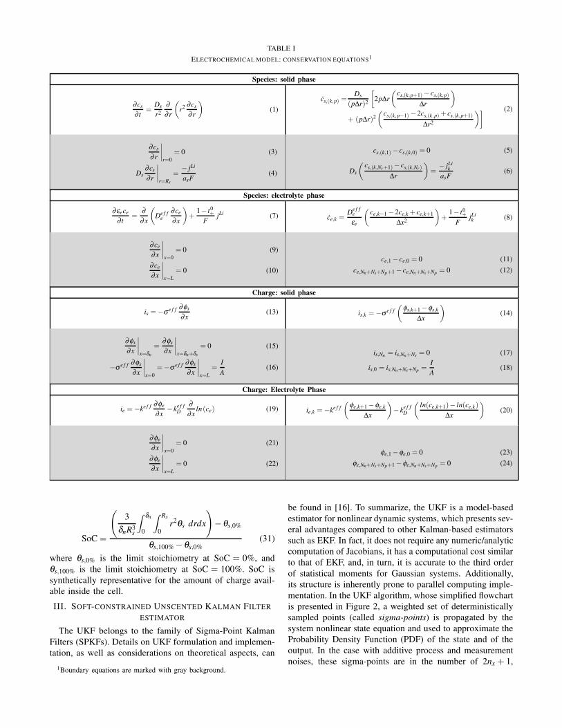
TABLE I

ELECTROCHEMICAL MODEL: CONSERVATION EQUATIONS1

Species: solid phase

∂cs

∂ t=

Ds

r2

∂

∂ r

(

r2 ∂cs

∂ r

)

(1)

cs,(k,p) =Ds

(p∆r)2

[

2p∆r

(

cs,(k,p+1)− cs,(k,p)

∆r

)

+ (p∆r)2

(

cs,(k,p−1)−2cs,(k,p)+ cs,(k,p+1)

∆r2

)] (2)

∂cs

∂ r

∣

∣

∣

∣

r=0

= 0 (3)

Ds∂cs

∂ r

∣

∣

∣

∣

r=Rs

=− jLi

asF(4)

cs,(k,1)− cs,(k,0) = 0 (5)

Ds

(

cs,(k,Nr+1)− cs,(k,Nr )

∆r

)

=− jLi

k

asF(6)

Species: electrolyte phase

∂εece

∂ t=

∂

∂x

(

De f fe

∂ce

∂x

)

+1− t0

+

FjLi (7) ce,k =

De f fe

εe

(

ce,k−1 −2ce,k + ce,k+1

∆x2

)

+1− t0

+

FjLik (8)

∂ce

∂x

∣

∣

∣

∣

x=0

= 0 (9)

∂ce

∂x

∣

∣

∣

∣

x=L

= 0 (10)

ce,1 − ce,0 = 0 (11)

ce,Nn+Ns+Np+1 − ce,Nn+Ns+Np = 0 (12)

Charge: solid phase

is =−σ e f f ∂φs

∂x(13) is,k =−σ e f f

(

φs,k+1 −φs,k

∆x

)

(14)

∂φs

∂x

∣

∣

∣

∣

x=δn

=∂φs

∂x

∣

∣

∣

∣

x=δn+δs

= 0 (15)

−σ e f f ∂φs

∂x

∣

∣

∣

∣

x=0

=−σ e f f ∂φs

∂x

∣

∣

∣

∣

x=L

=I

A(16)

is,Nn = is,Nn+Ns = 0 (17)

is,0 = is,Nn+Ns+Np =I

A(18)

Charge: Electrolyte Phase

ie =−ke f f ∂φe

∂x− k

e f fD

∂

∂xln(ce) (19) ie,k =−ke f f

(

φe,k+1 −φe,k

∆x

)

− ke f fD

(

ln(ce,k+1)− ln(ce,k)

∆x

)

(20)

∂φe

∂x

∣

∣

∣

∣

x=0

= 0 (21)

∂φe

∂x

∣

∣

∣

∣

x=L

= 0 (22)

φe,1 −φe,0 = 0 (23)

φe,Nn+Ns+Np+1 −φe,Nn+Ns+Np = 0 (24)

SoC =

(

3

δnR3s

∫ δn

0

∫ Rs

0r2θs drdx

)

−θs,0%

θs,100% −θs,0%

(31)

where θs,0% is the limit stoichiometry at SoC = 0%, and

θs,100% is the limit stoichiometry at SoC = 100%. SoC is

synthetically representative for the amount of charge avail-

able inside the cell.

III. SOFT-CONSTRAINED UNSCENTED KALMAN FILTER

ESTIMATOR

The UKF belongs to the family of Sigma-Point Kalman

Filters (SPKFs). Details on UKF formulation and implemen-

tation, as well as considerations on theoretical aspects, can

1Boundary equations are marked with gray background.

be found in [16]. To summarize, the UKF is a model-based

estimator for nonlinear dynamic systems, which presents sev-

eral advantages compared to other Kalman-based estimators

such as EKF. In fact, it does not require any numeric/analytic

computation of Jacobians, it has a computational cost similar

to that of EKF, and, in turn, it is accurate to the third order

of statistical moments for Gaussian systems. Additionally,

its structure is inherently prone to parallel computing imple-

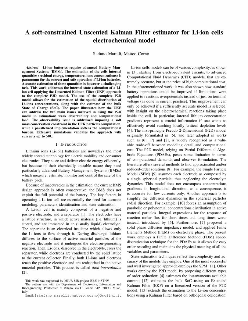
mentation. In the UKF algorithm, whose simplified flowchart

is presented in Figure 2, a weighted set of deterministically

sampled points (called sigma-points) is propagated by the

system nonlinear state equation and used to approximate the

Probability Density Function (PDF) of the state and of the

output. In the case with additive process and measurement

noises, these sigma-points are in the number of 2nx + 1,

New time step:� � � � 1

�� � ������

�� � �� � ����

Initialization:���. �. � ��� � � ���� � �������������

� computation�� � 0

Cell simulator (ODE 15s)� � ��. . �� � ����� � 0. . 2�

� computation

A-priori state estimate: ����

� computation

Output estimate: y��

Gain computation

A-posteriori state estimate: ����

Fig. 2. UKF algorithm simplified flowchart.

where nx is the dimension of the state vector; in the present

work, the state vector is composed of all discretized elements

of cs and ce, so nx = (Nr + 1)(Nn +Np) +Ns, as recalled

above. The initial dispersion of these points is ruled by the

covariance matrix P0 of the initial state estimate, which is

a tuning parameter. The covariance matrix Q of the process

disturbance and the covariance matrix R of the measurement

noise are also important tuning parameters. Minor UKF

tuning parameters description can be found elsewhere [14].

A. Weak observability of P2D model

The model presented in Section II suffers from poor ob-

servability of the concentration in the core of active material

particles from the output voltage, as already pointed out in

[11] for SPM. The weak observability of the P2D model is

confirmed by applying the classical UKF approach to the

discretized P2D model with Nr = 5 and Nn = Ns = Np = 3,

using current as an input and voltage as a measured output.

Figure 3 plots the estimated SoC during a current pulses

cycle. In the simulation, the UKF is initialized with 20%

SoC error. The figure shows that the filter does not converge.

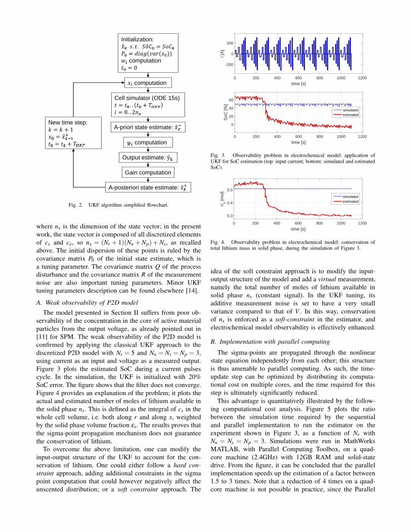
Figure 4 provides an explanation of the problem; it plots the

actual and estimated number of moles of lithium available in

the solid phase ns. This is defined as the integral of cs in the

whole cell volume, i.e. both along r and along x, weighted

by the solid phase volume fraction εs. The results proves that

the sigma-point propagation mechanism does not guarantee

the conservation of lithium.

To overcome the above limitation, one can modify the

input-output structure of the UKF to account for the con-

servation of lithium. One could either follow a hard con-

straint approach, adding additional constraints in the sigma

point computation that could however negatively affect the

unscented distribution; or a soft constraint approach. The

0 200 400 600 800 1000 1200

time [s]

-200

0

200

I [A

]

0 200 400 600 800 1000 1200

time [s]

0

20

40

60

SoC

[%]

simulatedestimated

Fig. 3. Observability problem in electrochemical model: application ofUKF for SoC estimation (top: input current; bottom: simulated and estimatedSoC).

0 200 400 600 800 1000 1200

time [s]

0.3

0.4

0.5

n s [mol

]

simulatedestimated

Fig. 4. Observability problem in electrochemical model: conservation oftotal lithium mass in solid phase, during the simulation of Figure 3.

idea of the soft constraint approach is to modify the input-

output structure of the model and add a virtual measurement,

namely the total number of moles of lithium available in

solid phase ns (constant signal). In the UKF tuning, its

additive measurement noise is set to have a very small

variance compared to that of V . In this way, conservation

of ns is enforced as a soft-constraint in the estimator, and

electrochemical model observability is effectively enhanced.

B. Implementation with parallel computing

The sigma-points are propagated through the nonlinear

state equation independently from each other; this structure

is thus amenable to parallel computing. As such, the time-

update step can be optimized by distributing its computa-

tional cost on multiple cores, and the time required for this

step is ultimately significantly reduced.

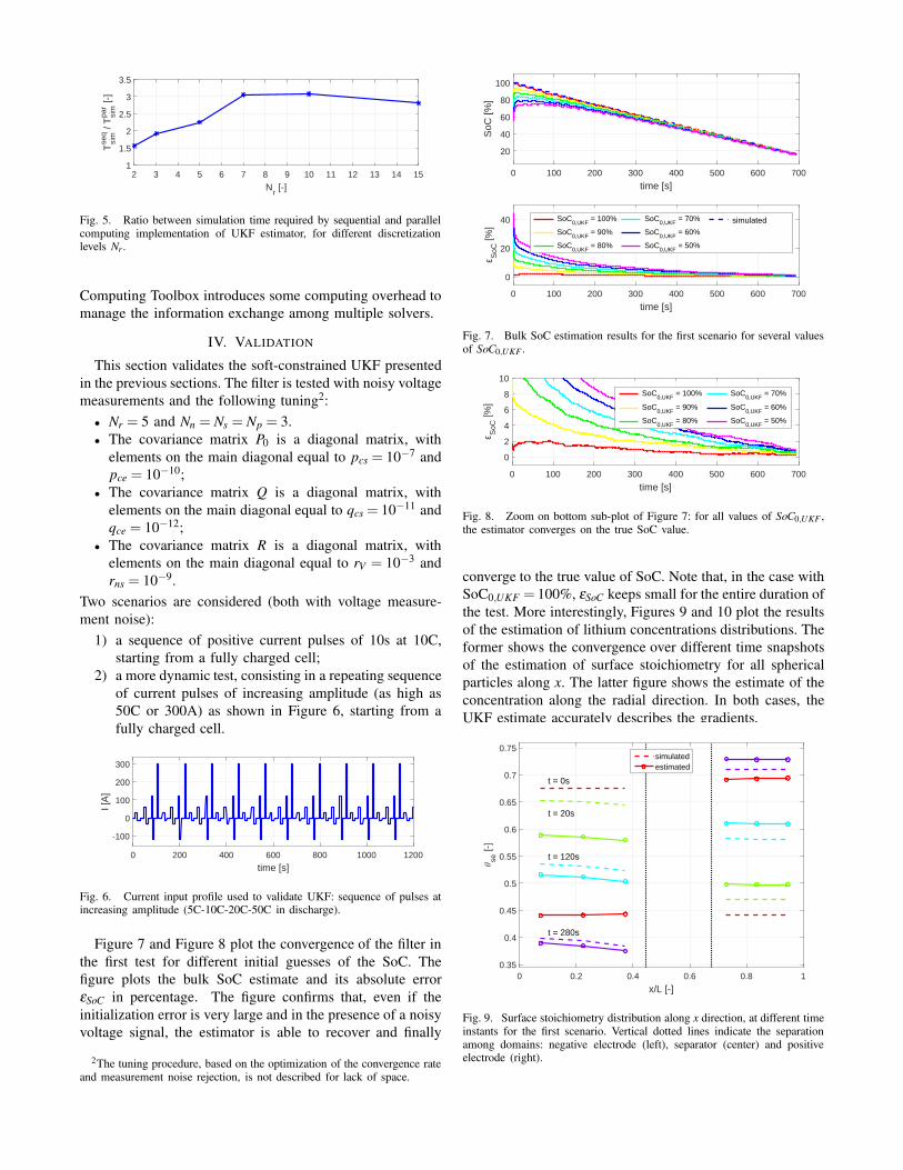
This advantage is quantitatively illustrated by the follow-

ing computational cost analysis. Figure 5 plots the ratio

between the simulation time required by the sequential

and parallel implementation to run the estimator on the

experiment shown in Figure 3, as a function of Nr with

Nn = Ns = Np = 3. Simulations were run in MathWorks

MATLAB, with Parallel Computing Toolbox, on a quad-

core machine (2.4GHz) with 12GB RAM and solid-state

drive. From the figure, it can be concluded that the parallel

implementation speeds up the estimation of a factor between

1.5 to 3 times. Note that a reduction of 4 times on a quad-

core machine is not possible in practice, since the Parallel

2 3 4 5 6 7 8 9 10 11 12 13 14 15

Nr [-]

1

1.5

2

2.5

3

3.5

Tsi

mse

q /

Tsi

mpa

r [-]

Fig. 5. Ratio between simulation time required by sequential and parallelcomputing implementation of UKF estimator, for different discretizationlevels Nr .

Computing Toolbox introduces some computing overhead to

manage the information exchange among multiple solvers.

IV. VALIDATION

This section validates the soft-constrained UKF presented

in the previous sections. The filter is tested with noisy voltage

measurements and the following tuning2:

• Nr = 5 and Nn = Ns = Np = 3.

• The covariance matrix P0 is a diagonal matrix, with

elements on the main diagonal equal to pcs = 10−7 and

pce = 10−10;

• The covariance matrix Q is a diagonal matrix, with

elements on the main diagonal equal to qcs = 10−11 and

qce = 10−12;

• The covariance matrix R is a diagonal matrix, with

elements on the main diagonal equal to rV = 10−3 and

rns = 10−9.

Two scenarios are considered (both with voltage measure-

ment noise):

1) a sequence of positive current pulses of 10s at 10C,

starting from a fully charged cell;

2) a more dynamic test, consisting in a repeating sequence

of current pulses of increasing amplitude (as high as

50C or 300A) as shown in Figure 6, starting from a

fully charged cell.

0 200 400 600 800 1000 1200

time [s]

-100

0

100

200

300

I [A

]

Fig. 6. Current input profile used to validate UKF: sequence of pulses atincreasing amplitude (5C-10C-20C-50C in discharge).

Figure 7 and Figure 8 plot the convergence of the filter in

the first test for different initial guesses of the SoC. The

figure plots the bulk SoC estimate and its absolute error

εSoC in percentage. The figure confirms that, even if the

initialization error is very large and in the presence of a noisy

voltage signal, the estimator is able to recover and finally

2The tuning procedure, based on the optimization of the convergence rateand measurement noise rejection, is not described for lack of space.

0 100 200 300 400 500 600 700

time [s]

20

40

60

80

100

SoC

[%]

0 100 200 300 400 500 600 700

time [s]

0

20

40

SoC

[%]

SoC0,UKF

= 100%

SoC0,UKF

= 90%

SoC0,UKF

= 80%

SoC0,UKF

= 70%

SoC0,UKF

= 60%

SoC0,UKF

= 50%

simulated

Fig. 7. Bulk SoC estimation results for the first scenario for several valuesof SoC0,UKF .

0 100 200 300 400 500 600 700

time [s]

0

2

4

6

8

10

SoC

[%]

SoC0,UKF

= 100%

SoC0,UKF

= 90%

SoC0,UKF

= 80%

SoC0,UKF

= 70%

SoC0,UKF

= 60%

SoC0,UKF

= 50%

Fig. 8. Zoom on bottom sub-plot of Figure 7: for all values of SoC0,UKF ,the estimator converges on the true SoC value.

converge to the true value of SoC. Note that, in the case with

SoC0,UKF = 100%, εSoC keeps small for the entire duration of

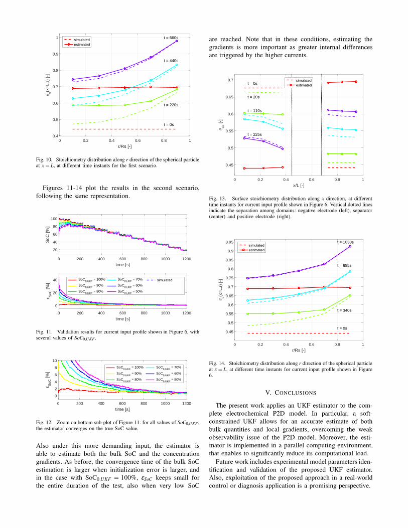
the test. More interestingly, Figures 9 and 10 plot the results

of the estimation of lithium concentrations distributions. The

former shows the convergence over different time snapshots

of the estimation of surface stoichiometry for all spherical

particles along x. The latter figure shows the estimate of the

concentration along the radial direction. In both cases, the

UKF estimate accurately describes the gradients.

0 0.2 0.4 0.6 0.8 1

x/L [-]

0.35

0.4

0.45

0.5

0.55

0.6

0.65

0.7

0.75

θse

[-]

t = 0s

t = 20s

t = 120s

t = 280s

simulatedestimated

Fig. 9. Surface stoichiometry distribution along x direction, at different timeinstants for the first scenario. Vertical dotted lines indicate the separationamong domains: negative electrode (left), separator (center) and positiveelectrode (right).

0 0.2 0.4 0.6 0.8 1

r/Rs [-]

0.4

0.5

0.6

0.7

0.8

0.9

1

θs(x

=L,

r) [-

]

t = 0s

t = 220s

t = 440s

t = 660ssimulatedestimated

Fig. 10. Stoichiometry distribution along r direction of the spherical particleat x = L, at different time instants for the first scenario.

Figures 11-14 plot the results in the second scenario,

following the same representation.

0 200 400 600 800 1000 1200

time [s]

20

40

60

80

100

SoC

[%]

0 200 400 600 800 1000 1200

time [s]

0

20

40

SoC

[%]

SoC0,UKF

= 100%

SoC0,UKF

= 90%

SoC0,UKF

= 80%

SoC0,UKF

= 70%

SoC0,UKF

= 60%

SoC0,UKF

= 50%

simulated

Fig. 11. Validation results for current input profile shown in Figure 6, withseveral values of SoC0,UKF .

0 200 400 600 800 1000 1200

time [s]

0

2

4

6

8

10

SoC

[%]

SoC0,UKF

= 100%

SoC0,UKF

= 90%

SoC0,UKF

= 80%

SoC0,UKF

= 70%

SoC0,UKF

= 60%

SoC0,UKF

= 50%

Fig. 12. Zoom on bottom sub-plot of Figure 11: for all values of SoC0,UKF ,the estimator converges on the true SoC value.

Also under this more demanding input, the estimator is

able to estimate both the bulk SoC and the concentration

gradients. As before, the convergence time of the bulk SoC

estimation is larger when initialization error is larger, and

in the case with SoC0,UKF = 100%, εSoC keeps small for

the entire duration of the test, also when very low SoC

are reached. Note that in these conditions, estimating the

gradients is more important as greater internal differences

are triggered by the higher currents.

0 0.2 0.4 0.6 0.8 1

x/L [-]

0.45

0.5

0.55

0.6

0.65

0.7

θse

[-]

t = 0s

t = 20s

t = 110s

t = 225s

simulatedestimated

Fig. 13. Surface stoichiometry distribution along x direction, at differenttime instants for current input profile shown in Figure 6. Vertical dotted linesindicate the separation among domains: negative electrode (left), separator(center) and positive electrode (right).

0 0.2 0.4 0.6 0.8 1

r/Rs [-]

0.45

0.5

0.55

0.6

0.65

0.7

0.75

0.8

0.85

0.9

0.95

θs(x

=L,

r) [-

]

t = 0s

t = 340s

t = 685s

t = 1030ssimulatedestimated

Fig. 14. Stoichiometry distribution along r direction of the spherical particleat x = L, at different time instants for current input profile shown in Figure6.

V. CONCLUSIONS

The present work applies an UKF estimator to the com-

plete electrochemical P2D model. In particular, a soft-

constrained UKF allows for an accurate estimate of both

bulk quantities and local gradients, overcoming the weak

observability issue of the P2D model. Moreover, the esti-

mator is implemented in a parallel computing environment,

that enables to significantly reduce its computational load.

Future work includes experimental model parameters iden-

tification and validation of the proposed UKF estimator.

Also, exploitation of the proposed approach in a real-world

control or diagnosis application is a promising perspective.

REFERENCES

[1] Karthik Somasundaram, Erik Birgersson, and Arun Sadashiv Mujum-dar. Thermal–electrochemical model for passive thermal managementof a spiral-wound lithium-ion battery. Journal of Power Sources,203:84–96, 2012.

[2] Nalin A Chaturvedi, Reinhardt Klein, Jake Christensen, Jasim Ahmed,and Aleksandar Kojic. Algorithms for advanced battery-managementsystems. IEEE Control Systems, 30(3):49–68, 2010.

[3] Paul WC Northrop, Bharatkumar Suthar, Venkatasailanathan Ramade-sigan, Shriram Santhanagopalan, Richard D Braatz, and Venkat RSubramanian. Efficient simulation and reformulation of lithium-ionbattery models for enabling electric transportation. Journal of The

Electrochemical Society, 161(8):E3149–E3157, 2014.[4] K. A. Smith, C. D. Rahn, and C. Y. Wang. Model-based electro-

chemical estimation and constraint management for pulse operationof lithium ion batteries. IEEE Transactions on Control Systems

Technology, 18(3):654–663, May 2010.[5] Marc Doyle, Thomas F Fuller, and John Newman. Modeling of

galvanostatic charge and discharge of the lithium/polymer/insertioncell. Journal of the Electrochemical Society, 140(6):1526–1533, 1993.

[6] Kandler Smith and Chao-Yang Wang. Solid-state diffusion limitationson pulse operation of a lithium ion cell for hybrid electric vehicles.Journal of Power Sources, 161(1):628–639, 2006.

[7] Kandler A Smith, Christopher D Rahn, and Chao-Yang Wang. Controloriented 1d electrochemical model of lithium ion battery. Energy

Conversion and management, 48(9):2565–2578, 2007.[8] Venkatasailanathan Ramadesigan, Vijayasekaran Boovaragavan, J Carl

Pirkle, and Venkat R Subramanian. Efficient reformulation of solid-phase diffusion in physics-based lithium-ion battery models. Journalof The Electrochemical Society, 157(7):A854–A860, 2010.

[9] Shriram Santhanagopalan, Qingzhi Guo, Premanand Ramadass, andRalph E White. Review of models for predicting the cycling perfor-mance of lithium ion batteries. Journal of Power Sources, 156(2):620–628, 2006.

[10] Venkat R Subramanian, Vinten D Diwakar, and Deepak Tapriyal.Efficient macro-micro scale coupled modeling of batteries. Journalof The Electrochemical Society, 152(10):A2002–A2008, 2005.

[11] Scott J Moura, Nalin A Chaturvedi, and Miroslav Krstic. Pdeestimation techniques for advanced battery management systems, parti: Soc estimation. In American Control Conference (ACC), 2012, pages559–565. IEEE, 2012.

[12] Matteo Corno, Nimitt Bhatt, Sergio M Savaresi, and Michel Verhae-gen. Electrochemical model-based state of charge estimation for li-ioncells. IEEE Transactions on Control Systems Technology, 23(1):117–127, 2015.

[13] Adrien M. Bizeray, Shi Zhao, Stephen Duncan, and David A. Howey.Lithium-ion battery thermal-electrochemical model-based state esti-mation using orthogonal collocation and a modified extended kalmanfilter. CoRR, abs/1506.08689, 2015.

[14] Gregory L Plett. Sigma-point kalman filtering for battery managementsystems of lipb-based hev battery packs: Part 1: Introduction and stateestimation. Journal of Power Sources, 161(2):1356–1368, 2006.

[15] Shriram Santhanagopalan and Ralph E. White. State of chargeestimation using an unscented filter for high power lithium ion cells.International Journal of Energy Research, 34(2):152–163, 2010.

[16] S. J. Julier, J. K. Uhlmann, and H. F. Durrant-Whyte. A new approachfor filtering nonlinear systems. In American Control Conference,

Proceedings of the 1995, volume 3, pages 1628–1632 vol.3, Jun 1995.