A Project Report on

Mathematica as a Tool for SolvingProblems in General Relativity

by

Tathagata KarmakarSB–1312043

under guidance of

Dr. Tapobrata Sarkar

Department of Physics

Indian Institute of Technology, Kanpur

July, 2016

Abstract

General theory of relativity provides us a new concept of gravity.Existence of gravitational waves, bending of starlight, precession ofplanetory orbits can be predicted using this theory. Beside all these,it is indispensable while exploring physics near a black hole. But itis extremely difficult, if not impossible, to solve Einstein’s equationsexactly. That’s why various computational tools like Mathematicaare becoming more useful day by day. This project explores Ferminormal coordinates near a Kerr metric and how Mathematica canbe used in efficient manner to explore physics in Kerr metric. Thebenefit of using Fermi normal coordinates will be emphasized throughexpression of tidal potential in that frame in Kerr metric.

i

Contents

Abstract i

Contents ii

List of Figures iii

1 Aim 1

2 Work 22.1 Part I: Studying general relativity . . . . . . . . . . . 22.2 Part II: Mathematica and RGTC package for calcula-

tions in general relativity . . . . . . . . . . . . . . . . 32.3 Part III: Kerr Spacetime Through Mathematica . . . 6

3 Results 12

4 Conclusions 16

5 Future Prospects 17

6 Acknowledgements 18

References 19

ii

List of Figures

2.1 Inputs & Commands for Running RGTC Package . . 42.2 Outputs after Running RGTC Package . . . . . . . . 52.3 Inputs & Commands for Kerr spacetime . . . . . . . 62.4 Standard Tetrad . . . . . . . . . . . . . . . . . . . . 72.5 Matrix and inverse matrix of tetrad components . . . 72.6 Code for calculation of Riemann tensor in tetrad frame 82.7 R(1)(2)(1)(2) . . . . . . . . . . . . . . . . . . . . . . . . 82.8 Calculating Q . . . . . . . . . . . . . . . . . . . . . . 92.9 Calculating P . . . . . . . . . . . . . . . . . . . . . . 92.10 Calculating P . . . . . . . . . . . . . . . . . . . . . . 102.11 P(a)(b)(1)(2)(1)(2) . . . . . . . . . . . . . . . . . . . . . . 102.12 Q(a)(1)(2)(1)(2) . . . . . . . . . . . . . . . . . . . . . . . 11

2.13 Λ and Λ̃ . . . . . . . . . . . . . . . . . . . . . . . . . 11

3.1 C̃ij, C̃ijk & B̃ijk . . . . . . . . . . . . . . . . . . . . . 13

3.2 C̃ijkl . . . . . . . . . . . . . . . . . . . . . . . . . . . 14

3.3 C̃3333 : Matches with 160 of [3] . . . . . . . . . . . . . 143.4 φtidal . . . . . . . . . . . . . . . . . . . . . . . . . . . 15

iii

Aim

The main objectives of the project are

• To learn the theory of general relativity beginning from the basicsand then studying application in case of a massive sphericallysymmetric star.

• To study the construction of Fermi normal coordinates and theirimportance.

• To learn use of RGTC package in Mathematica for calculationsin general relativity.

• To analyze the black hole tidal problem in Fermi normal coor-dinates with efficient algorithm in mathematica for the calcula-tions.

1

Work

2.1 Part I: Studying general relativity

First and foremost requirement of the project was being familiarwith general relativity. To fulfil this I had to study general raltivitybegining from the basics till some advanced topics. For most of thepart lecture notes of Matthias Blau were used [1]. Topics studiedwere:

I. Definition of tensor, tensor algebra, covariant derivatives of ten-sor, parallel transport, Fermi-Walker parallel transport [1, 2].

II. Definition of metric, geodesic equation, Christoffel symbols [1,2].

III. Principle of minimal coupling, energy-momentum tensor(of aperfect fluid), energy-momentum tensor as a source of gravity[1, 5].

IV. Riemann curvature tensor and its properties, geodesic deviationequation, Lie derivatives, Killing vectors(basics) [1].

V. Raychaudhuri equation for timelike geodesic congruences, Ray-chaudhuri equation for affine Null geodesic congruences, Ray-chaudhuri equation for non-affinely parametrized Null geodesics[1].

VI. Einstein’s equation, cosmological constant [1].

2

VII. Static, spherically symmetric metrics, Schwarzschild metric, Birkhoff’stheorem, interior solution for a static star, Tolman-Oppenheimer-Volkoff equation [1].

VIII. Equation for shape of orbit in Schwarzschild geometry, timelikeand null geodesics. Precession of perehelia of planetory orbits,bending of Light by a star [1].

IX. Schwarzschild radius, Schwarzschild black holes, Eddington-Finkelsteincoordinates, event horizons, Kruskal-Szekeres coordinates, max-imal extension of Schwarzschild spacetime [1].

X. Construction of Fermi normal coordinate system and Fermi nor-mal coordinate as local inertial frame( Mikowski metric andvanishing of Christoffel symbols) [6].

2.2 Part II: Mathematica and RGTC pack-age for calculations in general relativity

RGTC( Riemannian Geometry and Tensor Calculus) package forMathematica can be found in http://www.inp.demokritos.gr/~sbonano/

RGTC/. The file EDCRGTCcode.m should be kept in $Path of Math-ematica. Command �EDCRGTCcode.m loads the package.

To use the package one needs to define coordinates as a list of sym-bols and a symmetric matrix as metric. Then command RGten-sors[metric, coordinates] calculates the following( here U means up-per index and d means lower i.e. Γµαβ is denoted as GUdd[[µ,α,β]])∗:

• Metric gdd (also a input).

• Inverse metric gUU.

• Chrisoffel symbols.

∗See http://www.inp.demokritos.gr/~sbonano/RGTC/NEBX-RGTC.pdf

3

• Riemann tensors Rdddd i.e. Rµνρλ.

• Riemann tensors RUddd i.e. Rµνρλ.

• Ricci tensor Rdd.

• Scalar curvature R.

• Weyl tensor & Einstein tensors.

A sample run is shown below:

In[1]:=

In[2]:= H*Ishii, section III: COMPONENTS OF THE RIEMANN TENSOR FOR A KERR SPACETIME*LH*To be remembered that index 1 corresponds to temporal component and 2,

3,4 corresponds to 1,2,3 indices in Ishii's paper*L<< EDCRGTCcode.m

In[1]:= BLcoord = 8t, r, Θ, j<;H*Boyer-Lindquist coordinates*L

In[2]:= S = r^2 + a^2 Cos@ΘD^2; DD = r^2 + a^2 - 2 M r; simpRules = TrigRules;

H*Here D in Ishii's paper is written as DD*Lassmp =

HH2 r^2 + a^2 + a^2 Cos@2 ΘDL ³ 0L && HDD ³ 0L && H 2 S � 2 r^2 + a^2 + a^2 Cos@2 ΘDL && Hr >= 0L;

H*M and a denote mass and spin parameter respectively*L

In[3]:= gBL =

-1 + 2 M r � S 0 0 -2 M r a Sin@ΘD^2 � S

0 S � DD 0 0

0 0 S 0

-2 M r a Sin@ΘD^2 � S 0 0 HHr^2 + a^2L^2 - DD a^2 Sin@ΘD^2L Sin@ΘD^2 � S

;

In[4]:= RGtensors@gBL, BLcoordD;

gdd =

-1 +2 M r

r2+a2 Cos@ΘD2

0 0 -2 a M r Sin@ΘD2

r2+a2 Cos@ΘD2

0r2

+a2 Cos@ΘD2

a2-2 M r+r2

0 0

0 0 r2+ a2 Cos@ΘD2 0

-2 a M r Sin@ΘD2

r2+a2 Cos@ΘD2

0 0Sin@ΘD2 IIa2

+r2M2-a2 Ia2

-2 M r+r2M Sin@ΘD2Mr2

+a2 Cos@ΘD2

Figure 2.1: Inputs & Commands for Running RGTC Package

4

gdd =

-1 +2 M r

r2+a2 Cos@ΘD2

0 0 -2 a M r Sin@ΘD2

r2+a2 Cos@ΘD2

0r2

+a2 Cos@ΘD2

a2-2 M r+r2

0 0

0 0 r2+ a2 Cos@ΘD2 0

-2 a M r Sin@ΘD2

r2+a2 Cos@ΘD2

0 0Sin@ΘD2 IIa2

+r2M2-a2 Ia2

-2 M r+r2M Sin@ΘD2Mr2

+a2 Cos@ΘD2

LineElement =

Ir2+ a2 Cos@ΘD2M d@rD2

a2- 2 M r + r2

+

I2 M r - r2- a2 Cos@ΘD2M d@tD2

r2+ a2 Cos@ΘD2

+

Ir2+ a2 Cos@ΘD2M d@ΘD2

-

4 a M r d@tD d@jD Sin@ΘD2

r2+ a2 Cos@ΘD2

+

1

r2+ a2 Cos@ΘD2

d@jD2 Sin@ΘD2 Ia4+ 2 a2 r2

+ r4- a4 Sin@ΘD2

+ 2 a2 M r Sin@ΘD2- a2 r2 Sin@ΘD2M

gUU = :9-IIr2+ a2 Cos@ΘD2M Ia4

+ 2 a2 r2+ r4

- a4 Sin@ΘD2+ 2 a2 M r Sin@ΘD2

- a2 r2 Sin@ΘD2MM �I-2 a4 M r + a4 r2

- 4 a2 M r3+ 2 a2 r4

- 2 M r5+ r6

+ a6 Cos@ΘD2+ 2 a4 r2 Cos@ΘD2

+

a2 r4 Cos@ΘD2+ 2 a4 M r Sin@ΘD2

- a4 r2 Sin@ΘD2+ 4 a2 M r3 Sin@ΘD2

- a2 r4 Sin@ΘD2-

a6 Cos@ΘD2 Sin@ΘD2+ 2 a4 M r Cos@ΘD2 Sin@ΘD2

- a4 r2 Cos@ΘD2 Sin@ΘD2M, 0, 0,

I2 a M r Ir2+ a2 Cos@ΘD2MM � I2 a4 M r - a4 r2

+ 4 a2 M r3- 2 a2 r4

+ 2 M r5- r6

- a6 Cos@ΘD2-

2 a4 r2 Cos@ΘD2- a2 r4 Cos@ΘD2

- 2 a4 M r Sin@ΘD2+ a4 r2 Sin@ΘD2

- 4 a2 M r3 Sin@ΘD2+

a2 r4 Sin@ΘD2+ a6 Cos@ΘD2 Sin@ΘD2

- 2 a4 M r Cos@ΘD2 Sin@ΘD2+ a4 r2 Cos@ΘD2 Sin@ΘD2M=,

:0,a2

- 2 M r + r2

r2+ a2 Cos@ΘD2

, 0, 0>, :0, 0,1

r2+ a2 Cos@ΘD2

, 0>,

9I2 a M r Ir2+ a2 Cos@ΘD2MM � I2 a4 M r - a4 r2

+ 4 a2 M r3- 2 a2 r4

+ 2 M r5- r6

- a6 Cos@ΘD2-

2 a4 r2 Cos@ΘD2- a2 r4 Cos@ΘD2

- 2 a4 M r Sin@ΘD2+ a4 r2 Sin@ΘD2

- 4 a2 M r3 Sin@ΘD2+

a2 r4 Sin@ΘD2+ a6 Cos@ΘD2 Sin@ΘD2

- 2 a4 M r Cos@ΘD2 Sin@ΘD2+ a4 r2 Cos@ΘD2 Sin@ΘD2M,

0, 0, II2 M r - r2- a2 Cos@ΘD2M Ir2

+ a2 Cos@ΘD2M Csc@ΘD2M �I2 a4 M r - a4 r2

+ 4 a2 M r3- 2 a2 r4

+ 2 M r5- r6

- a6 Cos@ΘD2- 2 a4 r2 Cos@ΘD2

-

a2 r4 Cos@ΘD2- 2 a4 M r Sin@ΘD2

+ a4 r2 Sin@ΘD2- 4 a2 M r3 Sin@ΘD2

+ a2 r4 Sin@ΘD2+

a6 Cos@ΘD2 Sin@ΘD2- 2 a4 M r Cos@ΘD2 Sin@ΘD2

+ a4 r2 Cos@ΘD2 Sin@ΘD2M=>

gUU computed in 0.172 sec

Gamma computed in 0.125 sec

RiemannHddddL computed in 1.063 sec

RiemannHUdddL computed in 10.375 sec

Ricci computed in 2.609 sec

Weyl computed in 18.359 sec

Einstein computed in 5.625 sec

All tasks completed in 38.359 seconds

Figure 2.2: Outputs after Running RGTC Package

5

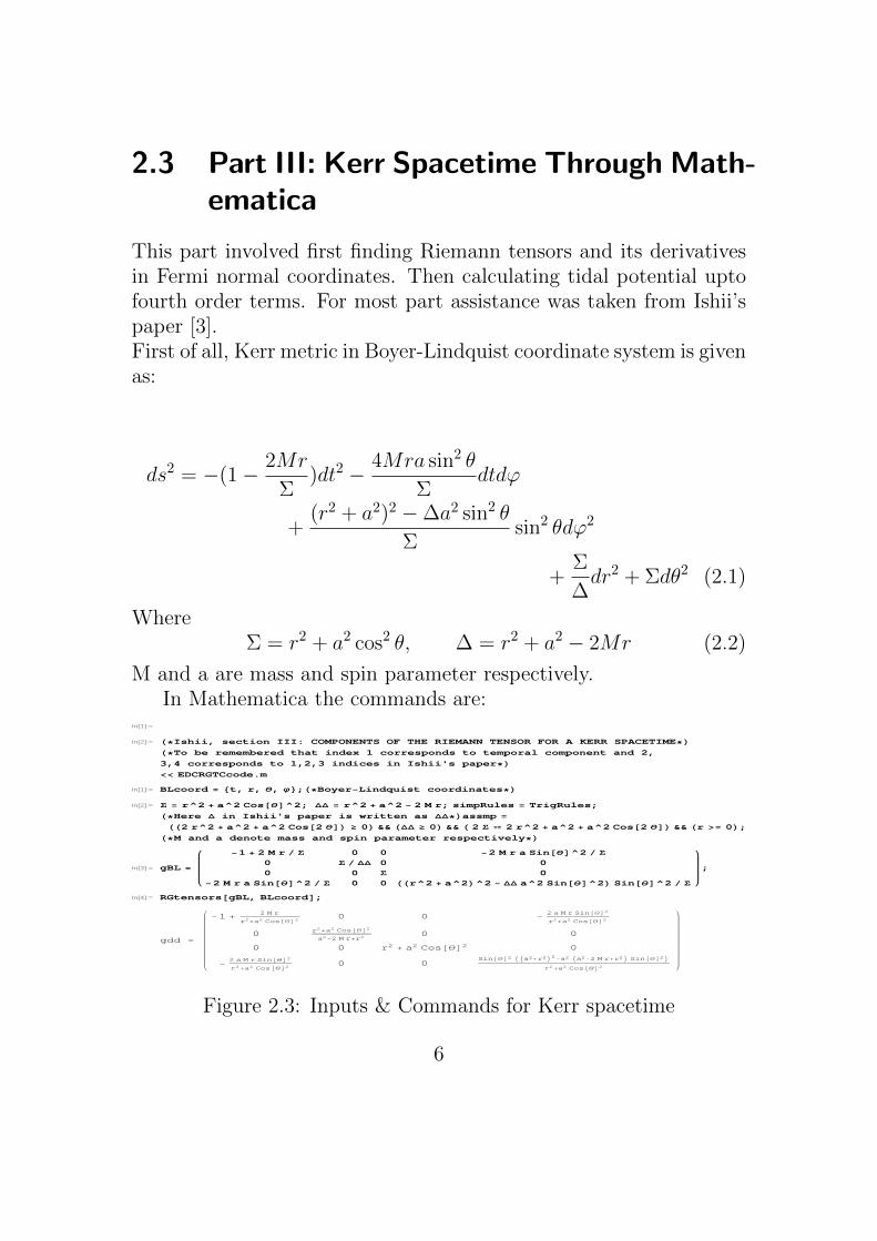
2.3 Part III: Kerr Spacetime Through Math-ematica

This part involved first finding Riemann tensors and its derivativesin Fermi normal coordinates. Then calculating tidal potential uptofourth order terms. For most part assistance was taken from Ishii’spaper [3].First of all, Kerr metric in Boyer-Lindquist coordinate system is givenas:

ds2 = −(1− 2Mr

Σ)dt2 − 4Mra sin2 θ

Σdtdϕ

+(r2 + a2)2 −∆a2 sin2 θ

Σsin2 θdϕ2

+Σ

∆dr2 + Σdθ2 (2.1)

WhereΣ = r2 + a2 cos2 θ, ∆ = r2 + a2 − 2Mr (2.2)

M and a are mass and spin parameter respectively.In Mathematica the commands are:

In[1]:=

In[2]:= H*Ishii, section III: COMPONENTS OF THE RIEMANN TENSOR FOR A KERR SPACETIME*LH*To be remembered that index 1 corresponds to temporal component and 2,

3,4 corresponds to 1,2,3 indices in Ishii's paper*L<< EDCRGTCcode.m

In[1]:= BLcoord = 8t, r, Θ, j<;H*Boyer-Lindquist coordinates*L

In[2]:= S = r^2 + a^2 Cos@ΘD^2; DD = r^2 + a^2 - 2 M r; simpRules = TrigRules;

H*Here D in Ishii's paper is written as DD*Lassmp =

HH2 r^2 + a^2 + a^2 Cos@2 ΘDL ³ 0L && HDD ³ 0L && H 2 S � 2 r^2 + a^2 + a^2 Cos@2 ΘDL && Hr >= 0L;

H*M and a denote mass and spin parameter respectively*L

In[3]:= gBL =

-1 + 2 M r � S 0 0 -2 M r a Sin@ΘD^2 � S

0 S � DD 0 0

0 0 S 0

-2 M r a Sin@ΘD^2 � S 0 0 HHr^2 + a^2L^2 - DD a^2 Sin@ΘD^2L Sin@ΘD^2 � S

;

In[4]:= RGtensors@gBL, BLcoordD;

gdd =

-1 +2 M r

r2+a2 Cos@ΘD2

0 0 -2 a M r Sin@ΘD2

r2+a2 Cos@ΘD2

0r2

+a2 Cos@ΘD2

a2-2 M r+r2

0 0

0 0 r2+ a2 Cos@ΘD2 0

-2 a M r Sin@ΘD2

r2+a2 Cos@ΘD2

0 0Sin@ΘD2 IIa2

+r2M2-a2 Ia2

-2 M r+r2M Sin@ΘD2Mr2

+a2 Cos@ΘD2

Figure 2.3: Inputs & Commands for Kerr spacetime

6

Standard tetrad is given as( see [3] eqns 74, 75, 76, 76):

In[5]:= H*Standard Tetrad*L

In[6]:= evec0 = 8Sqrt@DD � SD, 0, 0, -a Sin@ΘD^2 Sqrt@DD � SD<;

In[7]:= evec1 = 80, Sqrt@S � DDD, 0, 0<;

In[8]:= evec2 = 80, 0, Sqrt@SD, 0<;

In[9]:= evec3 = 8-a Sin@ΘD � Sqrt@SD, 0, 0, Hr^2 + a^2L Sin@ΘD � Sqrt@SD<;

In[10]:= H*To see they indeed are orthonormal*L8evec0.gUU.evec0, evec0.gUU.evec1, evec0.gUU.evec2, evec0.gUU.evec3< �� FullSimplify

Out[10]= 8-1, 0, 0, 0<

In[11]:= 8evec1.gUU.evec0, evec1.gUU.evec1, evec1.gUU.evec2, evec1.gUU.evec3< �� FullSimplify

Out[11]= 80, 1, 0, 0<

In[12]:= 8evec2.gUU.evec0, evec2.gUU.evec1, evec2.gUU.evec2, evec2.gUU.evec3< �� FullSimplify

Out[12]= 80, 0, 1, 0<

In[13]:= 8evec3.gUU.evec0, evec3.gUU.evec1, evec3.gUU.evec2, evec3.gUU.evec3< �� FullSimplify

Out[13]= 80, 0, 0, 1<

Figure 2.4: Standard Tetrad

The tetrad components (e(a)µ ) are written as a matrix named jac.

The matrix inverse is ijac (eµ(a)). R1dddd is full simplified form of

Rdddd (for computations with R1dddd will take lesser time thoughcomputation of R1dddd might take 2-3 minutes). A picture is shownin the next page.

In[14]:= jac = 8evec0, evec1, evec2, evec3<;H*Writing tetrad components eHaLΜ as matrix jac*L

In[15]:= ijac = FullSimplify@Inverse@jacD, assmpD;H*ijac consists of eHaLΜ*L

In[16]:=

In[17]:= H*R1dddd is Simplified version of Rdddd*LR1dddd = Table@FullSimplify@Rdddd@@i, j, k, lDD, assmpD,

8i, 1, 4<, 8j, 1, 4<, 8k, 1, 4<, 8l, 1, 4<D;

Figure 2.5: Matrix and inverse matrix of tetrad components

Calculation of components of Riemann tensor in tetrad frame isgiven on next page:

7

In[20]:= H*Below combpos creates all even combinations of first four inputs

and combneg creates odd combinations*Lcombpos@i_, j_, k_, l_, m___D :=

88i, j, k, l, m<, 8j, i, l, k, m<, 8k, l, i, j, m<, 8l, k, j, i, m<<;

In[21]:= combneg@i_, j_, k_, l_, m___D :=

88i, j, l, k, m<, 8j, i, k, l, m<, 8l, k, i, j, m<, 8k, l, j, i, m<<;

In[22]:= A = 8<;H*A is to be filled with independent combinations of type i-j-k-l*LIn[23]:= H*This function returns true if none of the combinations of input is already in A*L

check@i_, j_, k_, l_D :=

check@i, j, k, lD = H! MemberQ@A, 8i, j, l, k<DL && H! MemberQ@A, 8j, i, k, l<DL &&

H! MemberQ@A, 8j, i, l, k<DL && H! MemberQ@A, 8l, k, i, j<DL &&

H! MemberQ@A, 8k, l, i, j<DL && H! MemberQ@A, 8k, l, j, i<DL && H! MemberQ@A, 8l, k, j, i<DLIn[24]:= Do@A = If@check@i, j, k, lD, Append@A, 8i, j, k, l<D, AD,

8i, 1, 4<, 8j, 1, 4<, 8k, 1, 4<, 8l, 1, 4<D;

In[25]:= H*Calculation of tetrad components of Rdddd*LcalR@i_, j_, k_, l_D := calR@i, j, k, lD = If@i � j ÈÈ k � l, 0,

FullSimplify@Sum@R1dddd@@i1, i2, i3, i4DD ijac@@i1, iDD ijac@@i2, jDD ijac@@i3, kDDijac@@i4, lDD, 8i1, 1, 4<, 8i2, 1, 4<, 8i3, 1, 4<, 8i4, 1, 4<D, assmpDD;

In[26]:= Rlist = 8<;

In[27]:= Do@Rlist = Append@Rlist, calR@A@@iDD �. List ® SequenceDD, 8i, Length@AD<D;

In[28]:= Rtetrad@i_, j_, k_, l_D :=

Rtetrad@i, j, k, lD = If@Intersection@A, combpos@i, j, k, lDD ¹ 8<,

Rlist@@Position@A, Intersection@A, combpos@i, j, k, lDD@@1DDD@@1, 1DDDD,

-Rlist@@Position@A, Intersection@A, combneg@i, j, k, lDD@@1DDD@@1, 1DDDDD;

Figure 2.6: Code for calculation of Riemann tensor in tetrad frame

Results can be mathced with 78, 79 of [3].

In[88]:= Rtetrad@2, 3, 2, 3D

Out[88]=

M r I3 a2- 2 r2

+ 3 a2 Cos@2 ΘDM

2 Ir2+ a2 Cos@ΘD2M3

Figure 2.7: R(1)(2)(1)(2)

Here one must remember that temporal components has index 1in code. 1, 2, 3 spatial indices are written as 2, 3, 4 indices in code.In similar manner Q and P can be calculated( see [3] 80 to 99).

8

In[29]:= H* This calculates component ijklm of covariant derivative of R1dddd,

where m is differentiation index*LdefcR@i_, j_, k_, l_, m_D := defcR@i, j, k, l, mD = If@i � j ÈÈ k � l, 0, FullSimplify@

D@R1dddd@@i, j, k, lDD, BLcoord@@mDDD - Sum@GUdd@@n, m, iDD R1dddd@@n, j, k, lDD +

GUdd@@n, m, jDD R1dddd@@i, n, k, lDD + GUdd@@n, m, kDD R1dddd@@i, j, n, lDD +

GUdd@@n, m, lDD R1dddd@@i, j, k, nDD, 8n, 1, 4<D, assmpDD;

In[30]:= CA = 8<;H*CA will contain all independent 8i,j,k,l,m< *LIn[31]:= Do@CA = Append@CA, Append@A@@iDD, jDD, 8i, 1, Length@AD<, 8j, 1, 4<D;

In[32]:= coCA = 8<;

In[33]:= Do@coCA = Append@coCA, defcR@CA@@iDD �. List ® SequenceDD, 8i, Length@CAD<D;

In[34]:= corR@i_, j_, k_, l_, m_D :=

corR@i, j, k, l, mD = If@Intersection@CA, combpos@i, j, k, l, mDD ¹ 8<,

coCA@@Position@CA, Intersection@CA, combpos@i, j, k, l, mDD@@1DDD@@1, 1DDDD,

-coCA@@Position@CA, Intersection@CA, combneg@i, j, k, l, mDD@@1DDD@@1, 1DDDDD;

In[35]:= H*This function will return Q in tetrad frame as a vector: As written in the paper*LQ@i_, j_, k_, l_D :=

Q@i, j, k, lD = Q@j, i, l, kD = Q@k, l, i, jD = Q@l, k, j, iD = FullSimplify@Table@If@i � j ÈÈ k � l, 0, Sum@corR@i1, i2, i3, i4, i5D ijac@@i5, mDD ijac@@i1, iDD

ijac@@i2, jDD ijac@@i3, kDD ijac@@i4, lDD, 8i1, 1, 4<, 8i2, 1, 4<,

8i3, 1, 4<, 8i4, 1, 4<, 8i5, 1, 4<DD, 8m, 82, 3, 4, 1<<D, assmpD;

Figure 2.8: Calculating Q

In[36]:= CCA = 8<;H*CCA will be filled with independent components of 8i,j,k,l,m,n< *L

In[37]:= Do@CCA = Append@CCA, Append@CA@@iDD, jDD, 8i, 1, Length@CAD<, 8j, 1, 4<D;

In[38]:= co2CA = 8<;

In[39]:= pos@i_, j_, k_, l_, m_, n_D :=

pos@i, j, k, l, m, nD = If@Intersection@CCA, combpos@i, j, k, l, m, nDD ¹ 8<,

8Position@CCA, Intersection@CCA, combpos@i, j, k, l, m, nDD@@1DDD@@1, 1DD, 1<,

8Position@CCA, Intersection@CCA, combneg@i, j, k, l, m, nDD@@1DDD@@1, 1DD, -1<D;

Figure 2.9: Calculating P

9

In[40]:=

H* This calculates component ijklmn of double covariant derivative of R1dddd,

where m and n are succesive differentiation index*Ldef2cR@i_, j_, k_, l_, m_, n_D := def2cR@i, j, k, l, m, nD =

If@i � j ÈÈ k � l, 0, FullSimplify@HD@corR@i, j, k, l, mD, BLcoord@@nDDD -

Sum@GUdd@@q, n, iDD corR@q, j, k, l, mD + GUdd@@q, n, jDD corR@i, q, k, l, mD +

GUdd@@q, n, kDD corR@i, j, q, l, mD + GUdd@@q, n, lDD corR@i, j, k, q, mD +

GUdd@@q, n, mDD corR@i, j, k, l, qD, 8q, 1, 4<DL �. Θ ® Pi � 2, assmpDD;

In[41]:= cor2R@i_, j_, k_, l_, m_, n_D :=

cor2R@i, j, k, l, m, nD = co2CA@@pos@i, j, k, l, m, nD@@1DD DD pos@i, j, k, l, m, nD@@2DD;

In[42]:= calc2R@i_, j_, k_, l_, m_, n_D :=

calc2R@i, j, k, l, m, nD = If@pos@i, j, m, k, l, nD@@1DD < pos@i, j, k, l, m, nD@@1DD &&

pos@i, j, l, m, k, nD@@1DD < pos@i, j, k, l, m, nD@@1DD,

-cor2R@i, j, m, k, l, nD - cor2R@i, j, l, m, k, nD, def2cR@i, j, k, l, m, nDD;

In[43]:= Do@co2CA = Append@co2CA, calc2R@CCA@@iDD �. List ® SequenceDD, 8i, Length@CCAD<D;

In[44]:= ijac1 = FullSimplify@ijac �. Θ ® Pi � 2, assmpD;

H*P is calculated only on equatorial plane*LIn[45]:= H*This function will return P in tetrad frame as a vector: As written in the paper*L

P@i_, j_, k_, l_D := P@i, j, k, lD =

P@j, i, l, kD = P@k, l, i, jD = P@l, k, j, iD = Table@If@i � j ÈÈ k � l, 0, FullSimplify@Sum@H1 � 2L Hcor2R@i1, i2, i3, i4, i5, i6D + cor2R@i1, i2, i3, i4, i6, i5DL

ijac1@@i1, iDD ijac1@@i2, jDD ijac1@@i3, kDD ijac1@@i4, lDD ijac1@@i5, mDDijac1@@i6, nDD, 8i1, 1, 4<, 8i2, 1, 4<, 8i3, 1, 4<, 8i4, 1, 4<,

8i5, 1, 4<, 8i6, 1, 4<D, assmpDD, 8n, 82, 3, 4, 1<<, 8m, 82, 3, 4, 1<<D

Figure 2.10: Calculating P

Result can be matched:

Figure 2.11: P(a)(b)(1)(2)(1)(2)

10

In[90]:= Q@2, 3, 2, 3D

Out[90]= : 3 M a2+ r H-2 M + rL I-24 a2 r2

+ 8 r4+ 4 a2 Ia2

- 6 r2M Cos@2 ΘD + a4 H3 + Cos@4 ΘDLM �

I8 Ir2+ a2 Cos@ΘD2M9�2M,

3 a2 M r Ia2- 2 r2

+ a2 Cos@2 ΘDM Sin@2 ΘD

Ir2+ a2 Cos@ΘD2M9�2

, 0, 0>

Figure 2.12: Q(a)(1)(2)(1)(2)

Λ(a)a denotes components of the four vecotrs, used for construction

of Fermi normal coordinates, in tetrad frame. Components Λ̃( see100 to 147 in [3]) are also calculated.

Figure 2.13: Λ and Λ̃

11

Results

Tidal component of gravitational potential is given as( see 129 of[3]):

φtidal =1

2Cijx

ixj +1

6Cijkx

ixjxk +1

24[Cijkl + 4C(ijCkl)−

4B(kl|n|Bij)n]xixjxkxl +O(x5) (3.1)

Where i,j,k,l are summed over spatial components and∗

Cij = R0i0j, Cijk = R0(i|0|j;k), Cijkl = R0(i|0|j;kl), Bijk = Rk(ij)0

In tilde frame, assuming r � M(>a):

φtidal =1

2C̃ijx̃

ix̃j +1

6C̃ijkx̃

ix̃jx̃k +1

24[C̃ijkl + 4C̃(ijC̃kl)−

4B̃(kl|n|B̃ij)n]x̃ix̃jx̃kx̃l +O(x̃5) (3.2)

Code for calculating C̃ & B̃ components is given below:

∗Where first bracket means averaged over permutations.A(p1p2...|q1|...|q2|...pn) = 1

n!

∑permutationsApermutations of p with q fixed.

12

In[60]:= H*Riemann tensor in tilde frame*LcalRtilde@i_, j_, k_, l_D := calRtilde@i, j, k, lD = If@i � j ÈÈ k � l, 0,

FullSimplify@Sum@HRtetrad@i1, j1, k1, l1D �. Θ ® Pi � 2L mat@@i1, iDD mat@@j1, jDDmat@@k1, kDD mat@@l1, lDD, 8i1, 1, 4<, 8j1, 1, 4<, 8k1, 1, 4<, 8l1, 1, 4<DDD;

In[61]:= Rtildelist = 8<;

In[62]:= Do@Rtildelist = Append@Rtildelist, calRtilde@A@@iDD �. List ® SequenceDD, 8i, Length@AD<D;

In[63]:= Rtilde@i_, j_, k_, l_D := Rtilde@i, j, k, lD = If@Intersection@A, combpos@i, j, k, lDD ¹ 8<,

Rtildelist@@Position@A, Intersection@A, combpos@i, j, k, lDD@@1DDD@@1, 1DDDD,

-Rtildelist@@Position@A, Intersection@A, combneg@i, j, k, lDD@@1DDD@@1, 1DDDDD;

In[64]:= Ctilde@i_, j_D := Ctilde@i, jD = Rtilde@1, i, 1, jD;

In[65]:= Btilde@i_, j_, k_D := Btilde@i, j, kD = H1 � 2L HRtilde@k, i, j, 1D + Rtilde@k, j, i, 1DL;

In[66]:= perm@ls_ListD :=

Module@8n = 0, htemp = 8<, m = 0<, n = Length@lsD; htemp = Permutations@Range@nDD;

m = Length@htempD; Table@ls@@htemp@@i, jDDDD, 8i, m<, 8j, n<DDIn[67]:= QA = CA;

In[68]:= calQ@i_, j_, k_, l_, m_D :=

calQ@i, j, k, l, mD = calQ@j, i, l, k, mD = calQ@k, l, i, j, mD = calQ@l, k, j, i, mD =

If@i � j ÈÈ k � l, 0, FullSimplify@Sum@HcorR@i1, i2, i3, i4, i5D �. Θ ® Pi � 2Lijac1@@i5, mDD ijac1@@i1, iDD ijac1@@i2, jDD ijac1@@i3, kDD ijac1@@i4, lDD,

8i1, 1, 4<, 8i2, 1, 4<, 8i3, 1, 4<, 8i4, 1, 4<, 8i5, 1, 4<DDD;

Figure 3.1: C̃ij, C̃ijk & B̃ijk

Calculating C̃ijkl needs extra care because we have to find a wayto calculate sum of all combination of indices of double covariantderivative of Riemann tensor. The code is shown on next page.

13

In[69]:= coRtilde@i_, j_, k_, l_, m_D :=

coRtilde@i, j, k, l, mD = coRtilde@j, i, l, k, mD = coRtilde@k, l, i, j, mD =

coRtilde@l, k, j, i, mD = If@i � j ÈÈ k � l, 0, FullSimplify@Sum@calQ@i1, j1, k1, l1, m1D mat@@i1, iDD mat@@j1, jDD mat@@k1, kDD mat@@l1, lDD mat@@

m1, mDD, 8i1, 1, 4<, 8j1, 1, 4<, 8k1, 1, 4<, 8l1, 1, 4<, 8m1, 1, 4<DDD;

In[70]:= Ctilde@i_, j_, k_D := Ctilde@i, j, kD =

Module@8temp = 8<, len = 1, s = 0<, temp = perm@8i, j, k<D; len = Length@tempD;

Do@s = s + coRtilde@1, temp@@l, 1DD, 1, temp@@l, 2DD, temp@@l, 3DDD, 8l, len<D;

FullSimplify@s � lenDD;

In[71]:= calP@i_, j_, k_, l_, m_, n_D := calP@i, j, k, l, m, nD =

calP@j, i, l, k, m, nD = calP@k, l, i, j, m, nD = calP@l, k, j, i, m, nD =

If@i � j ÈÈ k � l, 0, Module@8m1 = 1, n1 = 1<, m1 = Which@m � 1, 4, m > 1, m - 1D;

n1 = Which@n � 1, 4, n > 1, n - 1D; P@i, j, k, l, m1, n1DDD;

In[72]:= co2Rtilde@i_, j_, k_, l_, m_, n_D :=

co2Rtilde@i, j, k, l, m, nD = co2Rtilde@j, i, l, k, m, nD =

co2Rtilde@k, l, i, j, m, nD = co2Rtilde@l, k, j, i, m, nD = If@i � j ÈÈ k � l, 0,

FullSimplify@Sum@HcalP@i1, j1, k1, l1, m1, n1D mat@@i1, iDD mat@@j1, jDDmat@@k1, kDD mat@@l1, lDD mat@@m1, mDD mat@@n1, nDDL,

8i1, 1, 4<, 8j1, 1, 4<, 8k1, 1, 4<, 8l1, 1, 4<, 8m1, 1, 4<, 8n1, 1, 4<DDD;

In[73]:= H@i_, j_, k_, l_, m_, n_D := H@i, j, k, l, m, nD = P@i, j, k, lD@@m, nDD;

In[74]:= Ctilde@i_, j_, k_, l_D := Ctilde@i, j, k, lD =

Module@8temp = 8<, len = 1, s = 0<, temp = perm@8i, j, k, l<D; len = Length@tempD;

Do@s = s + co2Rtilde@1, temp@@m, 1DD, 1, temp@@m, 2DD, temp@@m, 3DD, temp@@m, 4DDD,

8m, len<D; FullSimplify@Hs � lenL �. P ® HDD;

Figure 3.2: C̃ijkl

In[75]:= Ctilde@4, 4, 4, 4D

Out[75]= -

1

r93 M 3 a2 I2 B2

+ r2M + 6 a B 1 +

B2

r2r a2

+ r H-2 M + rL + r I3 r2 H-2 M + rL + B2 H-7 M + 3 rLM

Figure 3.3: C̃3333 : Matches with 160 of [3]

14

With these C̃ & B̃ we get (3.2). As shown:

In[76]:= xtilde = 8y0, y1, y2, y3<;

In[78]:= Φ1tidal = FullSimplify@Sum@H1 � 2L H Ctilde@i, jD �. B ® 0L xtilde@@iDD xtilde@@jDD, 8i, 82, 3, 4<<, 8j, 82, 3, 4<<DD;

In[79]:= Φ2tidal =

FullSimplify@Sum@H1 � 6L H Ctilde@i, j, kD �. B ® 0L xtilde@@iDD xtilde@@jDD xtilde@@kDD,

8i, 82, 3, 4<<, 8j, 82, 3, 4<<, 8k, 82, 3, 4<<DD �. Sqrt@a^2 + r H-2 M + rLD ® r;

In[80]:= Φ31tidal =

FullSimplify@Expand@FullSimplify@Sum@H1 � 24L H Ctilde@i, j, k, lD �. B ® 0L xtilde@@iDDxtilde@@jDD xtilde@@kDD xtilde@@lDD, 8i, 82, 3, 4<<,

8j, 82, 3, 4<<, 8k, 82, 3, 4<<, 8l, 82, 3, 4<<DD �. a ® 0D �. M ^2 ® 0D;

In[81]:= Cproduct@i_, j_, k_, l_D :=

Cproduct@i, j, k, lD = Module@8sums = 0, pp = 8<, len = 1<, pp = perm@8i, j, k, l<D;

len = Length@ppD; H1 � lenL Do@sums = sums + HCtilde@pp@@m, 1DD, pp@@m, 2DDDCtilde@pp@@m, 3DD, pp@@m, 4DDD �. B ® 0L, 8m, len<D ; sumsD;

In[82]:= Φ32tidal = FullSimplify@Sum@H1 � 6L Cproduct@i, j, k, lD xtilde@@iDD xtilde@@jDD xtilde@@kDD xtilde@@lDD,

8i, 82, 3, 4<<, 8j, 82, 3, 4<<, 8k, 82, 3, 4<<, 8l, 82, 3, 4<<DD �. M ^2 ® 0;

In[83]:= Bsum@i_, j_, k_, l_D := Sum@Btilde@i, j, nD Btilde@k, l, nD �. B ® 0, 8n, 82, 3, 4<<D

In[84]:= Bproduct@i_, j_, k_, l_D := Bproduct@i, j, k, lD =

Module@8sums = 0, pp = 8<, len = 1<, pp = perm@8i, j, k, l<D; len = Length@ppD; H1 � lenLDo@sums = sums + Bsum@pp@@m, 1DD, pp@@m, 2DD, pp@@m, 3DD, pp@@m, 4DDD, 8m, len<D ; sumsD

In[85]:= Φ33tidal = FullSimplify@-Sum@H1 � 6L Bproduct@i, j, k, lD xtilde@@iDD xtilde@@jDD xtilde@@kDD xtilde@@lDD,

8i, 82, 3, 4<<, 8j, 82, 3, 4<<, 8k, 82, 3, 4<<, 8l, 82, 3, 4<<DD �. M ^2 ® 0;

In[86]:= Φtidal = Φ1tidal + Φ2tidal + Φ31tidal + Φ32tidal + Φ33tidal

Out[86]=

M I-2 y12+ y22

+ y32M

2 r3+

M y1 I2 y12- 3 Iy22

+ y32MM

2 r4-

M I8 y14- 24 y12 Iy22

+ y32M + 3 Iy22+ y32M2M

8 r5

Figure 3.4: φtidalHere, x̃ is written as y. Code reproduces result 165 of Ishii’s paper[3].Thus, through Mathematica we have been able to calculate tidalpotential in Fermi normal coordinate system in Kerr spacetime.This result can be used for further calculations.

15

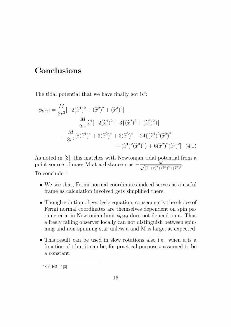
Conclusions

The tidal potential that we have finally got is∗:

φtidal =M

2r3[−2(x̃1)2 + (x̃2)2 + (x̃3)2]

− M

2r4x̃1[−2(x̃1)2 + 3{(x̃2)2 + (x̃3)2}]

− M

8r5[8(x̃1)4 + 3(x̃2)4 + 3(x̃3)4 − 24{(x̃1)2(x̃2)2

+ (x̃1)2(x̃3)2}+ 6(x̃2)2(x̃3)2] (4.1)

As noted in [3], this matches with Newtonian tidal potential from apoint source of mass M at a distance r as − M√

(x̃1+r)2+(x̃2)2+(x̃3)2.

To conclude :

• We see that, Fermi normal coordinates indeed serves as a usefulframe as calculation involved gets simplified there.

• Though solution of geodesic equation, consequently the choice ofFermi normal coordinates are themselves dependent on spin pa-rameter a, in Newtonian limit φtidal does not depend on a. Thusa freely falling observer locally can not distinguish between spin-ning and non-spinning star unless a and M is large, as expected.

• This result can be used in slow rotations also i.e. when a is afunction of t but it can be, for practical purposes, assumed to bea constant.

∗See 165 of [3]

16

Future Prospects

The whole work done throughout summer is a part of a bigger projectwhich will run throughout semester I of academic year 2016-17. Thispart is mainly comprised of learning relevant theory and Mathemat-ica. The ultimate goal of the project is to calculate tidal disruptionrate of stars near naked singularity and I hope I will get some reallyuseful and interesting results at the end. Beside this, in future, Iwish to study physics near a black hole more rigorously. Also, if Iget any chance, I wish to explore origin of gravitational waves neara black hole and using computaional tools I would like to build asimulation for that.

17

Acknowledgements

I sincerely express gratitude to my mentor Dr. Tapobrata Sarkarfor giving me this valuable opportunity to learn under him. He hasprovided immeasurable amount of support and guidance throghoutthe project. I would like to thank my friend Mr. Amartya Saha withwhom I frequently had discussions on theoritical topics. These dis-cussions led me to clearer understanding of the subject. I also thankMr. Ravindra Kumar Verma, Ph.D. student of our department, forhelping me with LATEX. Finally, I pay respect to my parents andelder sister for keeping me motivated throughout the project.

18

References

[1] Matthias Blau. Lecture notes on general relativity. December 15, 2015. http://www.blau.itp.unibe.ch/newlecturesGR.pdf

[2] I.S. Sokolnikoff. Tensor Analysis Theory and Applications. Applied Mathemat-ics Series. NEW YORK. JOHN WILEY & SONS, INC. LONDON. CHAP-MAN & HALL, LIMITED, 1951.

[3] M. Ishii, M. Shibata and Y. Mino, Phys. Rev. D 71, 044017 (2005).

[4] Thomas A. Moore. A General Relativity Workbook. University Science Books.Mill Valley, California.

[5] A good discussion on energy-momentum tensor can be found athttp://www2.warwick.ac.uk/fac/sci/physics/current/teach/module_

home/px436/notes/lecture6.pdf.

[6] F.K. Manasse and C.W. Misner. Journal of Mathematical Physics 4, 735(1963).

[7] J.A. Marck. Proceedings of the Royal Soceity of London. Series A, Mathemat-ical and Physical Sciences, Vol. 385, No. 1789 (Fb. 8, 1983), pp. 431-438.

[8] James M. Bardeen, William H. Press and Saul A. Teukolsky. The AstrophysicalJournal, 178:347-369, 1972.

[9] Mathematica tutorial at https://www.wolfram.com/learningcenter/

tutorialcollection/CoreLanguage/CoreLanguage.pdf.

[10] Roozbeh Hazrat. Mathematica: A Problem Centered Approach. Springer.

[11] The complete Mathematica code is available at https://drive.google.

com/file/d/0B3yQpROHCwaRTmJ4bUVxSGJSdHM/view?usp=sharing.

19