Embed Size (px)
Citation preview

A Practical Introduction to Regression
Discontinuity Designs: Volume II
Matias D. Cattaneo∗ Nicolas Idrobo† Rocıo Titiunik‡
June 14, 2018
Monograph prepared for
Cambridge Elements: Quantitative and Computational Methods for Social Science
Cambridge University Press
http://www.cambridge.org/us/academic/elements/
quantitative-and-computational-methods-social-science
** PRELIMINARY AND INCOMPLETE – COMMENTS WELCOME **
∗Department of Economics and Department of Statistics, University of Michigan.†Department of Economics, University of Michigan.‡Department of Political Science, University of Michigan.

CONTENTS CONTENTS
Contents
Acknowledgments 1
1 Introduction 3
2 The Local Randomization Approach to RD Analysis 9
2.1 Local Randomization Approach: Overview . . . . . . . . . . . . . . . . . . . 10
2.2 Local Randomization Estimation and Inference . . . . . . . . . . . . . . . . 15
2.2.1 Finite Sample Methods . . . . . . . . . . . . . . . . . . . . . . . . . . 16
2.2.2 Large Sample Methods . . . . . . . . . . . . . . . . . . . . . . . . . . 21
2.2.3 The Effect of Islamic Representation on Female Educational Attainment 23
2.2.4 Estimation and Inference in Practice . . . . . . . . . . . . . . . . . . 27
2.3 How to Choose the Window . . . . . . . . . . . . . . . . . . . . . . . . . . . 33
2.4 Falsification Analysis In The Local Randomization Approach . . . . . . . . . 47
2.4.1 Predetermined Covariates and Placebo Outcomes . . . . . . . . . . . 48
2.4.2 Density of Running Variable . . . . . . . . . . . . . . . . . . . . . . . 53
2.4.3 Placebo Cutoffs . . . . . . . . . . . . . . . . . . . . . . . . . . . . . . 55
2.4.4 Sensitivity to Window Choice . . . . . . . . . . . . . . . . . . . . . . 55
2.5 When To Use The Local Randomization Approach . . . . . . . . . . . . . . 56
2.6 Further Readings . . . . . . . . . . . . . . . . . . . . . . . . . . . . . . . . . 56
3 RD Designs with Discrete Running Variables 58
3.1 The Effect of Academic Probation on Future Academic Achievement . . . . 58
3.2 Counting the Number of Mass Points in the RD Score . . . . . . . . . . . . . 60
3.3 Using the Continuity-Based Approach when the Number of Mass Points isLarge . . . . . . . . . . . . . . . . . . . . . . . . . . . . . . . . . . . . . . . . 63
3.4 Interpreting Continuity-Based RD Analysis with Mass Points . . . . . . . . . 71
3.5 Local Randomization RD Analysis with Discrete Score . . . . . . . . . . . . 73
3.6 Further Readings . . . . . . . . . . . . . . . . . . . . . . . . . . . . . . . . . 80
4 The Fuzzy RD Design 82
4.1 Empirical Application: The Effect of Cash Transfers on Birth Weight . . . . 84
4.2 Continuity-based Analysis . . . . . . . . . . . . . . . . . . . . . . . . . . . . 86
i

CONTENTS CONTENTS
4.2.1 Empirical Example . . . . . . . . . . . . . . . . . . . . . . . . . . . . 89
4.3 Further Readings . . . . . . . . . . . . . . . . . . . . . . . . . . . . . . . . . 90
5 The Multi-Cutoff RD Design 91
5.1 Empirical Application . . . . . . . . . . . . . . . . . . . . . . . . . . . . . . 91
5.2 Taxonomy of Multiple Cutoffs . . . . . . . . . . . . . . . . . . . . . . . . . . 91
5.3 Local Polynomial Analysis . . . . . . . . . . . . . . . . . . . . . . . . . . . . 94
5.4 Local Randomization Analysis . . . . . . . . . . . . . . . . . . . . . . . . . . 94
5.5 Further Readings . . . . . . . . . . . . . . . . . . . . . . . . . . . . . . . . . 94
6 The Multi-Score RD Design 94
6.1 The General Setup . . . . . . . . . . . . . . . . . . . . . . . . . . . . . . . . 94
6.2 The Geographic RD Design . . . . . . . . . . . . . . . . . . . . . . . . . . . 96
6.2.1 Empirical Application . . . . . . . . . . . . . . . . . . . . . . . . . . 98
6.3 Further Readings . . . . . . . . . . . . . . . . . . . . . . . . . . . . . . . . . 98
7 Final Remarks 99
Bibliography 100
ii

ACKNOWLEDGMENTS CONTENTS
Acknowledgments
This monograph, together with its accompanying first part (Cattaneo, Idrobo and Titiu-
nik, 2018a), collects and expands the instructional materials we prepared for more than 30
short courses and workshops on Regression Discontinuity (RD) methodology taught over
the years 2014–2017. These teaching materials were used at various institutions and pro-
grams, including the Asian Development Bank, the Philippine Institute for Development
Studies, the International Food Policy Research Institute, the ICPSR’s Summer Program in
Quantitative Methods of Social Research, the Abdul Latif Jameel Poverty Action Lab, the
Inter-American Development Bank, the Georgetown Center for Econometric Practice, and
the Universidad Catolica del Uruguay’s Winter School in Methodology and Data Analysis.
The materials were also employed for teaching at the undergraduate and graduate level at
Brigham Young University, Cornell University, Instituto Tecnologico Autonomo de Mexico,
Pennsylvania State University, Pontificia Universidad Catolica de Chile, University of Michi-
gan, and Universidad Torcuato Di Tella. We thank all these institutions and programs, as
well as their many audiences, for the support, feedback and encouragement we received over
the years.
The work collected in our two-volume monograph evolved and benefited from many in-
sightful discussions with our present and former collaborators: Sebastian Calonico, Robert
Erikson, Juan Carlos Escanciano, Max Farrell, Yingjie Feng, Brigham Frandsen, Sebastian
Galiani, Michael Jansson, Luke Keele, Marko Klasnja, Xinwei Ma, Kenichi Nagasawa, Bren-
dan Nyhan, Jasjeet Sekhon, Gonzalo Vazquez-Bare, and Jose Zubizarreta. Their intellectual
contribution to our research program on RD designs has been invaluable, and certainly made
our monographs much better than they would have been otherwise. We also thank Alberto
Abadie, Joshua Angrist, Ivan Canay, Richard Crump, David Drukker, Sebastian Galiani,
Guido Imbens, Patrick Kline, Justin McCrary, David McKenzie, Douglas Miller, Aniceto
Orbeta, Zhuan Pei, and Andres Santos for the many stimulating discussions and criticisms
we received from them over the years, which also shaped the work presented here in important
ways. The co-Editors Michael Alvarez and Nathaniel Beck offered useful and constructive
comments on a preliminary draft of our manuscript, including the suggestion of splitting
the content into two stand-alone volumes. Last but not least, we gratefully acknowledge the
support of the National Science Foundation through grant SES-1357561.
The goal of our two-part monograph is purposely practical and hence we focus on the
empirical analysis of RD designs. We do not seek to provide a comprehensive literature review
on RD designs nor discuss theoretical aspects in detail. In this second part, we employ the
1

ACKNOWLEDGMENTS CONTENTS
data of Meyersson (2014), Lindo, Sanders and Oreopoulos (2010), Amarante, Manacorda,
Miguel and Vigorito (2016), Chay, McEwan and Urquiola (2005) and Keele and Titiunik
(2015) for empirical illustration of the different topics covered. We thank these authors
for making their data and codes publicly available. We provide complete replication codes
in both R and Stata for all the empirical work discussed throughout the monograph. In
addition, we provide replication codes for another empirical illustration using the data of
Cattaneo, Frandsen and Titiunik (2015), which is not discussed in the text to conserve space
and because it is already analyzed in our companion software articles. The general purpose,
open-source software used in this monograph, as well as other supplementary materials, can
be found at:
https://sites.google.com/site/rdpackages/
2

1. INTRODUCTION CONTENTS
1 Introduction
The Regression Discontinuity (RD) design has emerged as one of the most credible research
designs in the social, behavioral, biomedical and statistical sciences for program evaluation
and causal inference in the absence of experimental treatment assignment. In this manuscript
we continue the discussion given in Cattaneo, Idrobo and Titiunik (2018a), the first part of
our two-part monograph offering a practical introduction to the analysis and interpretation
of RD designs. While the present manuscript is meant to be self-contained, it is advisable to
consult Part I of our two-part monograph as several concepts and ideas discussed previously
will naturally feature in this volume.
The RD design is defined by three fundamental ingredients: a score (also known as running
variable, forcing variable, or index), a cutoff, and a treatment rule that assigns units to
treatment or control based on a hard-thresholding rule using the score and cutoff. All units
are assigned a score, and a treatment is assigned to those units whose value of the score
exceeds the cutoff and not assigned to units whose value of the score is below the cutoff.
This treatment assignment rule implies that the probability of treatment assignment changes
abruptly at the known cutoff. If units are not able to perfectly determine or manipulate
the exact value of the score that they receive, this discontinuous change in the treatment
assignment probability can be used to study the effect of the treatment on outcomes of
interest, at least locally, because units with scores barely below the cutoff can be used as
counterfactuals for units with scores barely above it.
In the accompanying Part I of our monograph (Cattaneo, Idrobo and Titiunik, 2018a),
we focused exclusively on the canonical Sharp RD design, where the running variable is
continuous and univariate, there is a single cutoff determining treatment assignment and
treatment compliance is perfect, and the analysis is conducted using continuity-based meth-
ods (e.g., local polynomial approximations). To be more precise, assume that there are n
units, indexed by i = 1, 2, . . . , n, and each unit receives score Xi. Units with Xi ≥ x are
assigned to the treatment condition, and units with Xi < x are assigned to the untreated or
control condition, where x denotes the RD cutoff. Thus, in the canonical Sharp RD design,
the univariate Xi is continuously distributed (i.e., all units received different values), and all
units comply with their treatment assignment.
We denote treatment assignment by Ti = 1(Xi ≥ x), where 1(·) is the indicator function.
In the canonical RD treatment assignment rule is deterministic, once the score is assigned
to each unit, and obeyed by all units (perfect treatment compliance). More generally, the
key defining feature of any RD design is that the probability of treatment assignment given
3

1. INTRODUCTION CONTENTS
the score changes discontinuously at the cutoff, that is, the conditional probability of being
assigned to treatment given the score, P(Ti = 1|Xi = x), jumps discontinuously at the cutoff
point x = x. Figure 1.1a illustrates this graphically.
Figure 1.1: Canonical Sharp RD Design
Assigned to TreatmentAssigned to Control
Cutoff
0
0.5
1
cScore (X)
Con
ditio
nal P
roba
bilit
y of
Rec
eivi
ng T
reat
men
t
(a) Conditional Probability of Treatment
E[Y(1)|X]
E[Y(0)|X]
Cutoff
τSRD
●
●
µ+
µ−
cScore (X)
E[Y
(1)|
X],
E[Y
(0)|
X]
(b) RD Treatment Effect
We adopt the potential outcomes framework to discuss causal inference and policy eval-
uation employing RD designs; see Imbens and Rubin (2015) for an introduction to potential
outcomes and causality, and Abadie and Cattaneo (2018) for a review of program evaluation
methodology. Each unit has two potential outcomes, Yi(1) and Yi(0), which correspond, re-
spectively, to the outcomes that would be observed under treatment or control. Treatment
effects are therefore defined in terms of comparisons between features of (the distribution
of) both potential outcomes, such as their means, variances or quantiles. If unit i receives
the treatment, we observe the unit’s outcome under treatment, Yi(1), but Yi(0) remains un-
observed, while if unit i is assigned to the control condition, we observe Yi(0) but not Yi(1).
This is known as the fundamental problem of causal inference. The observed outcome Yi is
therefore defined as
Yi = (1− Ti) · Yi(0) + Ti · Yi(1) =
{Yi(0) if Xi < x
Yi(1) if Xi ≥ x.
The canonical Sharp RD design, discussed in our prior monograph (Cattaneo, Idrobo and
4

1. INTRODUCTION CONTENTS
Titiunik, 2018a), assumes that the potential outcomes (Yi(1), Yi(0))ni=1 are random variables,
and focuses on the average treatment effect at the cutoff
τSRD ≡ E[Yi(1)− Yi(0)|Xi = x].
This (causal) parameter is sometimes called the Sharp RD treatment effect, and is depicted
in Figure 1.1b. In that figure we also plot the regression functions E[Yi(0)|Xi = x] and
E[Yi(1)|Xi = x] for values of the score Xi = x, where solid and dashed lines correspond to
their estimable and non-estimable portions, respectively. The continuity-based framework
for RD analysis, assumes that the regression functions E[Yi(1)|Xi = x] and E[Yi(0)|Xi = x],
seen as functions of x, are continuous at x = x, which gives
τSRD = limx↓x
E[Yi|Xi = x]− limx↑x
E[Yi|Xi = x]. (1.1)
In words, Equation 1.1 says that, if the average potential outcomes are continuous functions
of the score at x, the difference between the limits of the treated and control average observed
outcomes as the score approaches the cutoff is equal to the average treatment effect at the
cutoff. This identification result is due to Hahn, Todd and van der Klaauw (2001), and has
spiked a large body of methodological work on identification, estimation, inference, graphical
presentation, and falsification/validation for many RD design settings. In our first volume we
focused exclusively on the canonical Sharp RD designs, and gave a practical introduction to
the methods developed by Lee (2008), McCrary (2008), Imbens and Kalyanaraman (2012),
Calonico, Cattaneo and Titiunik (2014b, 2015a), Calonico, Cattaneo and Farrell (2018b,a),
and Calonico, Cattaneo, Farrell and Titiunik (2018c), among others.
In the present Part II of our monograph, we offer a practical discussion of several topics
in RD methodology building on and extending the continuity-based analysis of the canonical
Sharp RD design. Our first goal in this manuscript is to introduce readers to an alternative
RD setup based on local randomization ideas that can be useful in some practical applica-
tions and complements the continuity-based approach to RD analysis. Then, employing both
continuity and local randomization approaches, we extend the canonical Sharp RD design
in multiple directions.
Section 2 discusses the local randomization framework for RD designs, where the as-
signment of score values is viewed as-if randomly assigned in a small window around the
cutoff, so that placement above or below the cutoff and hence treatment assignment can
be interpreted to be as-if experimental. This contrasts with the continuity-based approach,
where extrapolation to the cutoff plays a predominant role. Once this local randomization
5

1. INTRODUCTION CONTENTS
assumption is invoked, the analysis can proceed by using standard tools in the analysis of
experiments literature. This alternative approach, which we call the Local Randomization
RD approach, requires stronger assumptions than the continuity-based approach discussed
in Part I, and for this reason it is not always applicable. We discuss the main features of the
local randomization approach in Section 2 below, including how to interpret the required
assumptions, and how to perform estimation, inference, presentation and falsification within
this alternative framework.
Next, in Section 3, we discuss RD designs where the running variable is discrete instead
of continuous, and multiple units share the same value of the score. This situation is common
in applications. For example, universities’ Grade Point Average (GPA) are often calculated
up to one or two decimal places, and collecting data on all students in a college campus
would result in a dataset where hundreds or thousands of students would have the same
GPA. In the RD design, the existence of such “mass points” in the score variable often
requires to different methods, as the standard continuity-based methods discussed in Part I
are no longer generally applicable. In Section 3, we discuss when and why continuity-based
methods will be inadequate to analyze RD designs with discrete scores, and discuss how the
local randomization approach can be a useful alternative framework for analysis.
We continue in Section 4 with a discussion of the so-called Fuzzy RD design, where
compliance with treatment assignment is no longer perfect (in contrast to the Sharp RD
case). In other words, these are RD designs where some units above the cutoff fail to take
the treatment despite being assigned to take it, and/or some units below the cutoff take the
treatment despite being assigned to the untreated condition. Our discussion defines several
parameters of interest that can be recovered under noncompliance, and discusses how to
employ both continuity-based and local randomization approaches for analysis. We also
discuss the important issue of how to perform falsification analysis under noncompliance.
We devote the last two sections to generalize the assumption of a treatment assignment
rule that depends on a single score and a single cutoff. In Section 5, we discuss RD designs
with multiple running variables, which we refer to as Multi-Score RD designs. Such designs
occur, for example, when students must obtain a grade above a cutoff in two different exams
in order to receive a scholarship. In this case, the treatment rule is thus more general, requir-
ing that both scores be above the cutoff in order to receive the treatment. Another example
RD designs with multiple scores that is used frequently in applications is the Geographic
RD design, where assignment to treatment of interest changes discontinuously at the border
that separates two geographic areas. We discuss how to generalize the methods discussed
both in Part I and in the first sections of this monograph to the multiple-score case, and
6

1. INTRODUCTION CONTENTS
illustrate how to apply this methods with a Geographic RD example. Finally, in Section 6
we consider RD designs with multiple cutoffs, a setup where all units have a score value,
but different subsets of units face different cutoff values. In our discussion, we highlight how
the Multiple-Cutoff RD design can be recast as Multiple-Score RD design with two running
variables.
Each section in this manuscript illustrates the methods with a different empirical applica-
tion. In Section 2, we use the data provided by Meyersson (2014) to study the effect of Islamic
parties’ victory on the educational attainment of women in Turkey. This is the same empiri-
cal application employed in Part I to illustrate the analysis of the canonical continuity-based
Sharp RD design. In Section 3, we re-analyze the data in Lindo et al. (2010), who analyze the
effects of academic probation on subsequent academic achievement. In Section 4 we use the
data provided by Amarante et al. (2016) to study the effect of a social assistance program on
the birth weight of babies born to beneficiary mothers. In Section 5, we re-analyze the data
in Chay, McEwan and Urquiola (2005), who study the effect of a school improvement pro-
gram on test scores, where units in different geographic regions facing different cutoff values.
Finally, in Section 5, we re-analyze the Geographic RD design in Keele and Titiunik (2015),
where the focus is to analyze the effect of campaign ads on voter turnout. We hope that the
multiple empirical applications we re-analyze across multiple disciplines will be useful to a
wide range of researchers.
As in the companion Part I of our monograph Cattaneo, Idrobo and Titiunik (2018a),
all the RD methods we discuss and illustrate are implemented using various general-purpose
software packages, which are free and available for both R and Stata, two leading statistical
software environments in the social sciences. Each numerical illustration we present includes
an R command with its output, and the analogous Stata command that reproduces the
same analysis—though we omit the Stata output to avoid repetition. The local polynomial
methods for continuity-based RD analysis are implemented in the package rdrobust, which
is presented and illustrated in three companion software articles: Calonico, Cattaneo and
Titiunik (2014a), Calonico, Cattaneo and Titiunik (2015b) and Calonico, Cattaneo, Farrell
and Titiunik (2017). This package has three functions specifically designed for continuity-
based RD analysis: rdbwselect for data-driven bandwidth selection methods, rdrobust for
local polynomial point estimation and inference, and rdplot for graphical RD analysis. In
addition, the package rddensity, discussed by Cattaneo, Jansson and Ma (2018c), provides
manipulation tests of density discontinuity based on local polynomial density estimation
methods. The accompanying package rdlocrand, which is presented and illustrated by Cat-
taneo, Titiunik and Vazquez-Bare (2016b), implements the local randomization methods
7

1. INTRODUCTION CONTENTS
discussed in the second part accompanying this monograph (Cattaneo, Idrobo and Titiunik,
2018b).
The full R and Stata codes that replicate all our analysis are available at https://sites.
google.com/site/rdpackages/replication. In that website, we also provide replication
codes for two other empirical applications, both following closely our discussion. One employs
the data on U.S. Senate incumbency advantage originally analyzed by Cattaneo, Frandsen
and Titiunik (2015), while the other uses the Head Start data originally analyzed by Ludwig
and Miller (2007) and recently employed in Cattaneo, Titiunik and Vazquez-Bare (2017).
Finally, we remind the reader that our main goal is not to offer a comprehensive review of
the literature on RD methodology (we do offer references to further readings after each topic
is presented), but rather to provide an accessible practical guide for empirical RD analysis.
For early review articles on RD designs see Imbens and Lemieux (2008) and Lee and Lemieux
(2010), and for an edited volume with a contemporaneous overview of the RD literature see
Cattaneo and Escanciano (2017). We are currently working on a comprehensive literature
review that complements our practical two-part monograph (Cattaneo and Titiunik, 2018).
8

2. LOCAL RANDOMIZATION RD APPROACH CONTENTS
2 The Local Randomization Approach to RD Analysis
In the first monograph (Cattaneo et al., 2018a), we discuss in detail the continuity-based
approach to RD analysis. This approach, which is based on assumptions of continuity (and
further smoothness) of the regression functions E[Yi(1)|Xi = x] and E[Yi(0)|Xi = x], is by
now the standard and most widely used method to analyze RD designs in practice. In this
section, we discuss a different framework for RD analysis that is based on a formalization
of the idea that the RD design can be interpreted as a sort of randomized experiment near
the cutoff x. This alternative framework can be used as a complement and robustness check
to the continuity-based analysis when the running variable is continuous, and is the most
natural framework when the running variable is discrete and has few mass points, a case we
discuss extensively in Section 3 below.
When the RD design was first introduced by Thistlethwaite and Campbell (1960), the
justification for this novel research design was not based on approximation and extrapolation
of smooth regression functions, but rather on the idea that the abrupt change in treatment
status that occurs at the cutoff leads to a treatment assignment mechanism that, near the
cutoff, resembles the assignment that we would see in a randomized experiment. Indeed, the
authors described a hypothetical experiment where the treatment is randomly assigned near
the cutoff as an “experiment for which the regression-discontinuity analysis may be regarded
as a substitute” (Thistlethwaite and Campbell, 1960, p. 310).
The idea that the treatment assignment is “as good as” randomly assigned in a neigh-
borhood of the cutoff is often invoked in the continuity-based framework to describe the
required identification assumptions in an intuitive way, and it has also been used to develop
formal results. However, within the continuity-based framework, the formal derivation of
identification and estimation results always relies on continuity and differentiability of re-
gression functions, and the idea of local randomization is used as a heuristic device only.
In contrast, what we call the local randomization approach to RD analysis formalizes that
idea that the RD design behaves like a randomized experiment near the cutoff by imposing
explicit randomization-type assumptions that are stronger than the standard continuity-type
conditions. In a nutshell, this approach imposes conditions so that units whose score values
lie in a small window around the cutoff can be analyzed as-if they were randomly assigned
to treatment or control. The local randomization approach adopts the local randomization
assumption explicitly, not as a heuristic interpretation, and builds a set of statistical tools
exploiting this specific assumption.
We now introduce the local randomization approach in detail, discussing how adopting
9

2. LOCAL RANDOMIZATION RD APPROACH CONTENTS
an explicit randomization assumption near the cutoff allows for the use of new methods of es-
timation and inference for RD analysis. We also discuss the differences between the standard
continuity-based approach and the local randomization approach. When the running vari-
able is continuous, the local randomization approach typically requires stronger assumptions
than the continuity-based approach; in these cases, it is natural to use the continuity-based
approach for the main RD analysis, and to use the local randomization approach as a ro-
bustness check. But in settings where the running variable is discrete (with few mass points)
or other departures from the canonical RD framework occur, the local randomization ap-
proach can not only be very useful but also possibly the only valid method for estimation
and inference in practice.
Recall that we are considering a RD design where the (continuos) score is Xi, the treat-
ment treatment assignment is Ti = 1(Xi ≥ x), Yi(1) and Yi(0) are the potential outcomes
under treatment and control, respectively, and Yi is the observed outcome. Throughout this
section, we maintain the assumption that the RD design is sharp—that is, we assume that
all units with score above the cutoff receive the treatment, and no units with score below
the cutoff receive it.
2.1 Local Randomization Approach: Overview
When the RD is based on a local randomization assumption, instead of assuming that the
unknown regression functions E[Yi(1)|Xi = x] and E[Yi(0)|Xi = x] are continuous at the
cutoff, the researcher assumes that there is a small window around the cutoff, W0 = [x−w0,
x + w0], such that for all units whose scores fall in that window their placement above or
below the cutoff is assigned as in a randomized experiment—an assumption that is sometimes
called as if random assignment. Formalizing the assumption that the treatment is (locally)
assigned as it would have been assigned in an experiment requires careful consideration of
the conditions that are guaranteed to hold in an actual experimental assignment.
There are important differences between the RD design and an actual randomized ex-
periment. To discuss such differences, we start by noting that any simple experiment can be
recast as an RD design where the score is a randomly generated number, and the cutoff is
chosen to ensure a certain treatment probability. For example, consider an experiment in a
student population that randomly assigns a scholarship with probability 1/2. This experi-
ment can be seen as an RD design where each student is assigned a random number with
uniform distribution between 0 and 100, say, and the scholarship is given to students whose
number or score is above 50. We illustrate this scenario in Figure 2.1(a).
10

2. LOCAL RANDOMIZATION RD APPROACH CONTENTS
The crucial feature of a randomized experiment recast as an RD design is that the
running variable, by virtue of being a randomly generated number, is unrelated to the average
potential outcomes. This is the reason why, in Figure 2.1(a), the average potential outcomes
E[Yi(1)|Xi = x] and E[Yi(0)|Xi = x] are constant for all values of x. Since the regression
functions are flat, the vertical distance between them can be recovered by the difference
between the average observed outcomes among all units in the treatment and control groups,
i.e. E[Yi|Xi ≥ 50]−E[Yi|Xi < 50] = E[Yi(1)|Xi ≥ 50]−E[Yi(0)|Xi < 50] = E[Yi(1)]−E[Yi(0)],
where the last equality follows from the assumption that Xi is a randomly generated number
and thus is unrelated to (i.e., independent of) Yi(1) and Yi(0).
Figure 2.1: Experiment versus RD Design
Cutoff
Average Treatment Effect
E[Y(1)|X]
E[Y(0)|X]
●
●
−1
0
1
2
−100 −50 x 50 100Score (X)
E[Y
(1)|
X],
E[Y
(0)|
X]
(a) Randomized Experiment
E[Y(1)|X]
E[Y(0)|X]
τSRD
Cutoff
●
●
−1
0
1
2
−100 −50 c 50 100Score (X)
E[Y
(1)|
X],
E[Y
(0)|
X]
(b) RD Design
In contrast, in the standard continuity-based RD design there is no requirement that
the potential outcomes be unrelated to the running variable over its support. Figure 2.1(b)
illustrates a standard continuity-based RD design where the average treatment effect at the
cutoff is the same as in the experimental setting in Figure 2.1(a), τSRD, but where the average
potential outcomes are non-constant functions of the score. This relationship between running
variable and potential outcomes is characteristic of many RD designs: since the score is often
related to the the units’ ability, resources, or performance (poverty index, vote shares, test
scores), units with higher scores are often systematically different from units whose scores
are lower. For example, a RD design where the score is a party’s vote share in a given election
and the outcome of interest is the party’s vote share in the following election, the overall
relationship between the score and the outcome will likely have a strongly positive slope,
11

2. LOCAL RANDOMIZATION RD APPROACH CONTENTS
as districts that strongly support the party in one election are likely to continue to support
the party in the near future. As illustrated in Figure 2.1(a), a nonzero slope in the plot of
E[Yi|Xi = x] against x does not occur in an actual experiment, because in an experiment x
is an arbitrary random number unrelated to the potential outcomes.
The crucial difference between the scenarios in Figures 2.1(a) and 2.1(b) is our knowl-
edge about the functional form of the regression functions. In a continuity-based approach,
the RD treatment effect in 2.1(b) can be estimated by calculating the limit of the average
observed outcomes as the score approaches the cutoff for the treatment and control groups,
limx↓x E[Yi|Xi = x]− limx↑x E[Yi|Xi = x]. The estimation of these limits requires that the re-
searcher approximate the regression functions, and this approximation will typically contain
an error that may directly affect estimation and inference. This is in stark contrast to the
experiment depicted in Figure 2.1(a), where the random assignment of the score implies that
the average potential outcomes are unrelated to the score and estimation does not require
functional form assumptions—by construction, the regression functions are constant in the
entire region where the score is randomly assigned.
A point often overlooked is that the known functional form of the regression functions
in a true experiment does not follow from the random assignment of the score per se, but
rather from the score being an arbitrary computer-generated number that is unrelated to the
potential outcomes. If the value of the score were randomly assigned but had a direct effect
on the average outcomes, the regression functions in Figure 2.1(a) would not necessarily be
flat. Thus, a local randomization approach to RD analysis must be based not only on the
assumption that placement above or below the cutoff is randomly assigned within a window
of the cutoff, but also on the assumption that the value of the score within this window is
unrelated to the potential outcomes—a condition that is guaranteed neither by the random
assignment of the score Xi, nor by the random assignment of the treatment Ti.
Formally, letting W0 = [x−w, x+w], the local randomization assumption can be stated
as the two following conditions:
(LR1) The distribution of the running variable in the window W0, FXi|Xi∈W0(x), is known, is
the same for all units, and does not depend on the potential outcomes: FXi|Xi∈W0(x) =
F (x)
(LR2) Inside W0, the potential outcomes depend on the running variable solely through the
treatment indicator Ti = 1(Xi ≥ x), but not directly: Yi(Xi, Ti) = Yi(Ti) for all i such
that Xi ∈ W0.
12

2. LOCAL RANDOMIZATION RD APPROACH CONTENTS
Under these conditions, inside the window W0, placement above or below the cutoff is
unrelated to the potential outcomes, and the potential outcomes are unrelated to the running
variable; therefore, the regression functions are flat inside W0. This is illustrated in Figure
2.2, where E[Yi(1)|Xi = x] and E[Yi(0)|Xi = x] are constant for all values of x inside W0,
but have non-zero slopes outside of it.
Figure 2.2: Local Randomization RD
E[Y(1)|X]
E[Y(0)|X]
Cutoff
τLR
− x−w0 x x + w0
Score (X)
E[Y
(1)|
X],
E[Y
(0)|
X]
The contrast between Figures 2.1(a), 2.1(b), and 2.2 illustrates the differences between
the actual experiment where the score is a randomly generated number, a continuity-based
RD design, and a local randomization RD design. In the actual experiment where the score
is a random number, the potential outcomes are unrelated to the score for all possible
score values—i.e., in the entire support of the score. In this case, there is no uncertainty
about the functional forms of E[Yi(1)|Xi = x] and E[Yi(0)|Xi = x]. In the continuity-based
13

2. LOCAL RANDOMIZATION RD APPROACH CONTENTS
RD design, the potential outcomes can be related to the score everywhere; the functions
E[Yi(1)|Xi = x] and E[Yi(0)|Xi = x] are completely unknown, and estimation and inference
is based on approximating them at the cutoff. Finally, in the local randomization RD design,
the potential outcomes can be related to the running variable far from the cutoff, but there
is a window around the cutoff where this relationship ceases. In this case, the functions
E[Yi(1)|Xi = x] and E[Yi(0)|Xi = x] are unknown over the entire support of the running
variable, but inside the window W0 they are assumed to be constant functions of x.
In some applications, assuming that the score has no effect on the (average) potential
outcomes near the cutoff may be regarded as unrealistic or too restrictive. However, such an
assumption can be taken as an approximation, at least for the very few units with scores
extremely close to the RD cutoff. As we will discuss below, a key advantage of the local
randomization approach is that it leads to valid and powerful finite sample inference methods,
which remain valid and can be used even when only a handful of observations very close to
the cutoff are included in the analysis.
Furthermore, the restriction that the score cannot directly affect the (average) potential
outcomes near the cutoff can be relaxed if the researcher is willing to impose more parametric
assumptions (locally to the cutoff). The local randomization assumption assumes that, inside
the window where the treatment is assumed to have been randomly assigned, the potential
outcomes are entirely unrelated to the running variable. This assumption, also known as
the exclusion restriction, leads to the flat regression functions in Figure 2.2. It is possible
to consider a slightly weaker version of this assumption where the potential outcomes are
allowed to depend on the running variable, but there exists a transformation that, once
applied to the potential outcomes of the units inside the window W0, leads to transformed
potential outcomes that are unrelated to the running variable.
More formally, the exclusion restriction in (LR2) requires that, for units with Xi ∈ W0,
the potential outcomes satisfy Yi(Xi, Ti) = Yi(Ti)—that is, the potential outcomes depend on
the running variable only via the treatment assignment indicator and not via the particular
value taken by Xi. In contrast, the weaker alternative assumption requires that, for units
with Xi ∈ W0, the exists a transformation φ(·) such that
φ(Yi(Xi, Ti), Xi, Ti) = Yi(Ti).
This condition says that, although the potential outcomes are allowed to depend on the
running variable Xi directly, the transformed potential outcomes Yi(Ti) depend only on the
treatment assignment indicator and thus satisfy the original exclusion restriction in (LR2).
14

2. LOCAL RANDOMIZATION RD APPROACH CONTENTS
For implementation, a transformation φ(·) must be assumed; for example, one can use a
polynomial of order p on the unit’s score, with slopes that are constant for all individuals
on the same side of the cutoff. This transformation has the advantage of linking the local
randomization approach to RD analysis to the continuity-based approach discussed in Part
I (Cattaneo et al., 2018a).
2.2 Local Randomization Estimation and Inference
Adopting a local randomization approach to RD analysis implies assuming that the as-
signment of units above or below the cutoff was random inside the window W0 (condition
LR1), and that in this window the potential outcomes are unrelated to the score (condition
LR2)—or can be somehow transformed to be unrelated to the score.
Therefore, given knowledge of W0, under a local randomization RD approach, we can
analyze the data as we would analyze an experiment. If the number of observations inside
W0 is large, researchers can use the full menu of standard large-sample experimental methods,
all of which are based on large-sample approximations—that is, on the assumption that the
number of units inside W0 is large enough to be well approximated by large sample limiting
distributions. These methods may or may not involve the assumption of random sampling,
and may or may not require LR2 per se (though removing LR2 will change the interpretation
of the RD parameter in general). In contrast, if the number of observations inside W0 is very
small, as it is often the case when local randomization methods are invoked in RD designs,
estimation and inference based on large-sample approximations may be invalid; in this case,
under appropriate assumptions, researchers can still employ randomization-based inference
methods that are exact in finite samples and do not require large-sample approximations
for their validity. These methods rely on the random assignment of treatment to construct
confidence intervals and hypothesis tests. We review both types of approaches below.
The implementation of experimental methods to analyze RD designs requires knowledge
or estimation of two important ingredients: (i) the window W0 where the local randomization
assumption is invoked; and (ii) the randomization mechanism that is needed to approximate
the assignment of units within W0 to the treatment and control conditions (i.e., to placement
above or below the cutoff). In real applications, W0 is fundamentally unknown and must be
selected by the research (ideally in an objective and data-driven way). Once W0 has been
estimated, the choice of the randomization mechanism can be guided by the structure of
the data, and it is not needed if large sample approximations are invoked. In most appli-
cations, the most natural assumption for the randomization mechanism is either complete
15

2. LOCAL RANDOMIZATION RD APPROACH CONTENTS
randomization or a Bernoulli assignment, where all units in W0 are assumed to have the same
probability of being placed above or below the cutoff. We first assume that W0 is known and
choose a particular random assignment mechanism inside W0. In Section 2.3, we discuss a
principled method to choose the window W0 in a data-driven way.
2.2.1 Finite Sample Methods
In many RD applications, a local randomization assumption will only be plausible in a very
small window around the cutoff, and by implication this small window will often contain very
few observations. In this case, it is natural to employ a Fisherian inference approach, which
is valid in any finite sample, and thus leads to correct inferences even when the number of
observations inside W0 is very small.
The Fisherian approach sees the potential outcomes as non-stochastic. This stands in con-
trast to the approach in the continuity-based RD framework, where the potential outcomes
are random variables as a consequence of random sampling. More precisely, in Fisherian
inference, the total number of units in the study, n, is seen as fixed—i.e., there is no random
sampling assumption; moreover, inferences do not rely on assuming that this number is large.
This setup is then combined with the so-called sharp null hypothesis that the treatment has
no effect for any unit:
HF0 : Yi(0) = Yi(1) for all i.
The combination of non-stochastic potential outcomes and the sharp null hypothesis
leads to inferences that are (type-I error) correct for any sample size because, under HF0,
both potential outcomes—Yi(1) and Yi(0)—can be imputed for every unit and there is no
missing data. In other words, under the sharp null hypothesis, the observed outcome of each
unit is equal to the unit’s two potential outcomes, Yi = Yi(1) = Yi(0). When the treatment
assignment is known, observing all potential outcomes are under the null hypothesis allows
us to derive the null distribution of any test statistic from the randomization distribution
of the treatment assignment alone. Since the latter distribution is finite-sample exact, the
Fisherian framework allows researchers to make inferences without relying on large-sample
approximations.
A hypothetical example
To illustrate how Fisherian inference leads to the exact distribution of test statistics, we
use a hypothetical example. We imagine that we have five units inside W0, and we randomly
assign nW0,+ = 3 units to treatment and nW0,− = nW0 − nW0,+ = 5− 3 = 2 units to control,
16

2. LOCAL RANDOMIZATION RD APPROACH CONTENTS
where nW0 is the total number of units inside W0. We choose the difference-in-means as the
test-statistic, Y+ − Y=1
nW0,+
∑i:i∈W0
YiTi + 1nW0,−
∑i:i∈W0
Yi(1− Ti). The treatment indicator
continues to be Ti, and we collect in the set TW0 all possible nW0-dimensional treatment
assignment vectors t within the window.
For implementation, we must choose a particular treatment assignment mechanism. In
other words, after assuming that placement above and below the cutoff was done as it would
have been done in an experiment, we must choose a particular randomization distribution
for the assignment. Of course, a crucial difference between an actual experiment and the
RD design is that, in the RD design, the true mechanism by which units are assigned a
value of the score smaller or larger than x inside W0 is fundamentally unknown. Thus, the
choice of the particular randomization mechanism is best understood as an approximation.
A common choice is the assumption that, within W0, nW0,+ units are assigned to treatment
and nW0 − nW0,+ units are assigned to control, where each unit has probability(nW0nW0,+
)−1of
being assigned to the treatment (i.e. above the cutoff) group. This is commonly known as
a complete randomization mechanism or a fixed margins randomization—under this mech-
anism, the number of treated and control units is fixed, as all treatment assignment vectors
result in exactly nW0,+ treated units and nW0 − nW0,+ control units.
In our example, under complete randomization, the number of elements in TW0 is(
53
)=
10—that is, there are ten different ways to assign five units to two groups of size three and
two. We assume that Yi(1) = 5 and Yi(0) = 2 for all units, so that the treatment effect,
Yi(1)− Yi(0), is constant and equal to 3 for all units. The top panel of Table 2.1 shows the
ten possible treatment assignment vectors, t1, . . . , t10, and the two potential outcomes for
each unit.
Suppose that the observed treatment assignment inside W0 is t6, so that units 1, 4 and 5
are assigned to treatment, and units 2 and 3 are assigned to control. Given this assignment,
the vector of observed outcomes is Y = (5, 2, 2, 5, 5), and the observed value of the difference-
in-means statistic is Sobs = Y+ − Y− = 5+5+53− 2+2
2= 5− 2 = 3. The bottom panel of Table
2.1 shows the distribution of the test statistic under the null—that is, the ten different
possible values that the difference-in-means can take when HF0 is assumed to hold. The
observed difference-in-means Sobs is the largest of the ten, and the exact p-value is therefore
pF = 1/10 = 0.10. Thus, we can reject HF0 with a test of level α = 0.10. Note that, since the
number of possible treatment assignments is ten, the smallest value that pF can take is 1/10.
This p-value is finite-sample exact, because the null distribution in Table 2.1 was derived
directly from the randomization distribution of the treatment assignment, and does not rely
on any statistical model or large-sample approximations.
17

2. LOCAL RANDOMIZATION RD APPROACH CONTENTS
Table 2.1: Hypothetical Randomization Distribution with Five Units
All Possible Treatment Assignments
Yi(1) Yi(0) t1 t2 t3 t4 t5 t6 t7 t8 t9 t10
Unit 1 5 2 1 1 1 1 1 1 0 0 0 0Unit 2 5 2 1 1 1 0 0 0 1 1 1 0Unit 3 5 2 1 0 0 1 1 0 1 1 0 1Unit 4 5 2 0 1 0 1 0 1 1 0 1 1Unit 5 5 2 0 0 1 0 1 1 0 1 1 1
Pr(T = t) 1/10 1/10 1/10 1/10 1/10 1/10 1/10 1/10 1/10 1/10
Distribution of Difference-in-Means When T = t6 and Y = (5, 2, 2, 5, 5)
Sobst1
Sobst2
Sobst3
Sobst4
Sobst5
Sobst6
Sobst7
Sobst8
Sobst9
Sobst10
Y+ 3 4 4 4 4 5 3 3 4 4Y− 5 3.5 3.5 3.5 3.5 2 5 5 3.5 3.5Y+ − Y− -2 0.5 0.5 0.5 0.5 3 -2 -2 0.5 0.5
Pr(S = Sobstj
) 1/10 1/10 1/10 1/10 1/10 1/10 1/10 1/10 1/10 1/10
This example illustrates that, in order to implement a local randomization RD analysis,
we need to specify, in addition to the choice of W0, the particular way in which the treatment
was randomized—that is, knowledge of the distribution of the treatment assignment. In
practice, the latter will not be known, but in many applications it can be approximated by
assuming a complete randomization within W0. Moreover, we need to choose a particular
test statistic; the difference-in-means is a simple choice, but below we discuss other options.
The General Fisherian Inference Framework
We can generalize the above example to provide a general formula for the exact p-value
associated with a test of HF. As before, we let TW0 be the treatment assignment for the
nW0 units in W0, and collect in the set TW0 all the possible treatment assignments that
can occur given the assumed randomization mechanism. In a complete or fixed margins
randomization, TW0 includes all vectors of length nW0 such that each vector has nW0,+ ones
and nW0,− = nW0 −nW0,+ zeros. Similarly, YW0 collects the nW0 observed outcomes for units
with Xi ∈ W0. We also need to choose a test statistic, which we denote S(TW0 ,YW0), that
is a function of the treatment assignment TW0 and the vector YW0 of observed outcomes for
the nW0 units in the experiment that is assumed to occur inside W0.
18

2. LOCAL RANDOMIZATION RD APPROACH CONTENTS
Of all the possible values of the treatment vector TW0 that can occur, only one will have
occurred in W0; we call this value the observed treatment assignment, tobsW0, and we denote
Sobs the observed value of the test-statistic associated with tobsW0, i.e. Sobs = t(tobsW0
,YW0). (In
the hypothetical example discussed above, we had tobsW0= t6.) Then, the one-sided finite-
sample exact p-value associated with a test of the sharp null hypothesis HF0 is the probability
that the test-static exceeds its observed value:
pF = P(S(TW0 ,YW0) ≥ Sobs) =∑
tW0∈TW0
1(S(tW0 ,YW0) ≥ Sobs) · P(TW0 = tW0).
When each of the treatment assignments in TW0 is equally likely, P(T = t) = 1#{TW0
} with
#{TW0} the number of elements in TW0 , and this expression simplifies to the number of times
the test-statistic exceeds the observed value divided by the total number of test-statistics
that can possibly occur,
pF = P(S(ZW0 ,YW0) ≥ Sobs) =# {S(tW0 ,YW0) ≥ Sobs}
#{TW0}.
Under the sharp null hypothesis, all potential outcomes are known and can be imputed. To
see this, note that under HF0 we have YW0 = YW0(1) = YW0(0), so that S(TW0 ,YW0) =
S(TW0 ,YW0(0)). Thus, under HF0, the only randomness in S(ZW0 ,YW0) comes from the
random assignment of the treatment, which is assumed to be known.
In practice, it often occurs that the total number of different treatment vectors tW0 that
can occur inside the windowW0 is too large, and enumerating them exhaustively is unfeasible.
For example, assuming a fixed-margins randomization inside W0 with 15 observations on each
side of the cutoff, there are(nW0nW0,t
)=(
3015
)= 155, 117, 520 possible treatment assignments,
and calculating pF by complete enumeration is very time consuming and possibly unfeasible.
When exhaustive enumeration is unfeasible, we can approximate pF using simulations, as
follows:
1. Calculate the observed test statistic, Sobs = S(tobsW0,YW0).
2. Draw a value tjW0from the treatment assignment distribution, P(TW0 ≤ tW0).
3. Calculate the test statistic for the jth draw tjW0, S(tjW0
,YW0).
4. Repeat steps 2 and 3 B times.
19
2. LOCAL RANDOMIZATION RD APPROACH CONTENTS
5. Calculate the simulation approximation to pF as
pF =1
B
B∑j=1
1(S(tjW0,YW0) ≥ Sobs).
Fisherian confidence intervals can be obtained by specifying sharp null hypotheses about
treatment effects, and then inverting these tests. In order to apply the Fisherian framework,
the null hypotheses to be inverted must be sharp—that is, under these null hypotheses, the
full profile of potential outcomes must be known. This requires specifying a treatment effect
model, and testing hypotheses about the specified parameters. A simple and common choice
is a constant treatment effect model, Yi(1) = Yi(0) + τ , which leads to the null hypothesis
HFτ0
: τ = τ0—note that HF0 is a special case of HF
τ0when τ0 = 0. Under this model, a 1 − α
confidence interval for τ can be obtained by collecting the set of all the values τ0 that fail to
be rejected when we test HFτ0
: τ = τ0 with an α-level test.
To test HFτ0
, we build test statistics based on an adjustment to the potential outcomes
that renders them constant under this null hypothesis. Under HFτ0
, the observed outcome is
Yi = Ti · Yi(1) + (1− Ti) · Yi(0)
= Ti · (Yi(0) + τ0) + (1− Ti) · Yi(0)
= Ti · τ0 + Yi(0).
Thus, the adjusted outcome Yi ≡ Yi−Tiτ0 = Yi(0) is constant under the null hypothesis HFτ0
.
A randomization-based test of HFτ0
proceeds by first calculating the adjusted outcomes Yi for
all the units in the window, and then computing the test statistic using the adjusted outcomes
instead of the raw outcomes, i.e. computing S(TW0 , YW0). Once the adjusted outcomes are
used to calculate the test statistic, we have S(TW0 , YW0) = S(TW0 ,YW0(0)) as before, and
a test of HFτ0
: τ = τ0 can be implemented as a test of the sharp null hypothesis HF0, using
S(ZW0 , YW0) instead of S(ZW0 ,YW0). We use pFτ0 to refer to the p-value associated with a
randomization-based test of HFτ0
.
In practice, assuming that τ takes values in [τmin, τmax], computing these confidence in-
tervals requires building a grid Gτ0 ={τ 1
0 , τ20 , . . . , τ
G0
}, with τ 1
0 ≥ τmin and τG0 ≤ τmax, and
collecting all τ0 ∈ Gτ0 that fail to be rejected with an α-level test of HFτ0
. Thus, the Fisherian
(1− α)× 100% confidence intervals is
CILRF ={τ0 ∈ Gτ0 : pFτ0 ≤ α
}.
20

2. LOCAL RANDOMIZATION RD APPROACH CONTENTS
The general principle of Fisherian inference is to use the randomization-based distribu-
tion of the test statistic under the sharp null hypothesis to derive p-values and confidence
intervals. In our hypothetical example, we illustrated the procedure using the difference-
in-means test statistic and the fixed margins randomization mechanism. But the Fisherian
approach to inference is general and works for any appropriate choice of test statistic and
randomization mechanism.
Other test statistics that could be used include the Kolmogorov-Smirnov (KS) statistic
and the Wilcoxon rank sum statistic. The KS statistic is defined as SKS = supy |F1(y)−F0(y)|,and measures the maximum absolute difference in the empirical cumulative distribution
functions (CDF) of the treated and control outcomes—denoted respectively by F1(·) and
F0(·). Because SKS is the treated-control difference in the outcome CDFs, it is well suited to
detect departures from the null hypothesis that involve not only differences in means but also
differences in other moments and in quantiles. Another test statistic commonly used is the
Wilcoxon rank sum statistic, which is based on the ranks of the outcomes, denoted Ryi . This
statistic is SWR =∑
i:Ti=1 Ryi , that is, it is the sum of the ranks of the treated observations.
Because SWR is based on ranks, it is not affected by the particular values of the outcome, only
by their ordering. Thus, unlike the difference-in-means, SWR is insensitive to outliers.
In addition to different choices of test statisics, the Fisherian approach allows for differ-
ent randomization mechanisms. An alternative to the complete randomization mechanism
discussed above is a Bernoulli assignment, where each unit is assigned to treatment with
some fixed equal probability. For implementation, researchers can set this probability equal
to 1/2 or, alternatively, equal to the proportion of treated units in W0. The disadvantage of
a Bernoulli assignment is that it can result in a treated or a control group with few or no
observations—a phenomenon that can never occur under complete randomization. However,
in practice, complete randomization and Bernoulli randomization often lead to very similar
conclusions for the same window W0.
2.2.2 Large Sample Methods
Despite the conceptual elegance of finite-sample Fisherian methods, the most frequently cho-
sen methods in the analysis of experiments are based on large-sample approximations. These
alternative methods are appropriate to analyze RD designs under a local randomization as-
sumption when the number of observations inside W0 is sufficiently large to ensure that the
moment and/or distributional approximations are sufficiently similar to the finite-sample
distributions of the statistics of interest.
21

2. LOCAL RANDOMIZATION RD APPROACH CONTENTS
A classic framework for experimental analysis is known as the Neyman approach. This ap-
proach relies on large-sample approximations to the randomization distribution of the treat-
ment assignment, but still assumes that the potential outcomes are fixed or non-stochastic.
In other words, the Neyman approach assumes that the sample size grows to infinity but
does not assume that the data is a (random) sample from a super-population. Unlike in
the Fisherian approach, in the Neyman framework point estimation is one of the main goals,
and the parameter of interest is typically the finite-sample average treatment effect. Inference
procedures in this framework usually focus on the null hypothesis that the average treatment
effect is zero.
To be more specific, consider the local randomization sharp RD effect, defined as
τ LRSRD = Y (1)− Y (0), Y (1) =1
nW0
∑i:Xi∈W0
Yi(1), Y (0) =1
nW0
∑i:Xi∈W0
Yi(0)
where Y (1) and Y (0) are the average potential outcomes inside the window. In this definition,
we have assumed that the potential outcomes are non-stochastic.
The parameter τ LRSRD is different from the more conventional continuity-based RD param-
eter τSRD defined in the introduction and discussed extensively in our companion Part I
monograph. While τ LRSRD is an average effect inside an interval (the window W0), τSRD is an
average at a single point (the cutoff x) where, by construction, the number of observations
is zero. This means that the decision to adopt a continuity-based approach versus a local
randomization approach directly affects the definition of the parameter of interest. Naturally,
if the window W0 is extremely small, τ LRSRD and τSRD become more conceptually similar.
Under the assumption of complete randomization inside W0, the observed difference-in-
means is an unbiased estimator of τ LRSRD. Thus a natural estimator for the RD effect τ LRSRD is the
difference between the average observed outcomes in the treatment and control groups,
τ LRSRD = Y+ − Y−, Y+ =1
nW0,+
∑i:Xi∈W0
Yi1(Xi ≥ x), Y− =1
nW0,−
∑i:Xi∈W0
Yi1(Xi < x),
where Y+ and Y− are the average treated and control observed outcomes inside W0 and, as be-
fore, nW0,+ and nW0,− are the number of treatment and control units inside W0, respectively.
In this case, a conservative estimator of the variance of τ LRSRD is given by V =σ2+
nW0,++
σ2−
nW0,−,
where σ2+ and σ2
− denote the sample variance of the outcome for the treatment and control
units within W0, respectively. A 100(1 − α)% confidence interval can be constructed in the
usual way by relying on a normal large-sample approximation to the randomization distri-
bution of the treatment assignment. For example, an approximate 95% confidence interval
22

2. LOCAL RANDOMIZATION RD APPROACH CONTENTS
is
CILRN =[τ LRSRD ± 1.96 ·
√V].
Hypothesis testing is based on Normal approximations. The Neyman null hypothesis is
HN0 : Y (1)− Y (0) = 0.
In contrast to Fisher’s sharp null hypothesis HF0, HN
0 does not allow us to calculate the full
profile of potential outcomes for every possible realization of the treatment assignment vector
t. Thus, unlike the Fisherian approach, the Neyman approach to hypothesis testing must
rely on approximation and is therefore not exact. In the Neyman approach, we can construct
the usual t-statistic using the point and variance estimators, S = Y+−Y−√V
, and then use the
Normal approximation to its distribution. For example, for a one-sided test, the p-value
associated with a test of HN0, is pN = 1− Φ(t), where Φ(·) is the Normal CDF.
Finally, it is possible to consider a setup where, in addition to using large-sample approx-
imations to the randomization mechanism as in the Neyman approach, the data {Yi, Xi}ni=1
is seen as random sample from a larger population—the same assumption made by the
continuity-based methods discussed in Cattaneo et al. (2018a). When random sampling
is assumed, the potential outcomes Yi(1) and Yi(0) are considered random variables, and
the units inside W0 are seen as a random sample from a (large) super-population. Be-
cause in this case the potential outcomes within W0 become stochastic by virtue of the
random sampling, the parameter of interest is the super-population average treatment ef-
fect, E[Yi(1)− Yi(0)|Xi ∈ W0]. Adopting this super-population perspective does not change
the Neyman estimation or inference procedures discussed above, though it does affect the
interpretation of the results.
2.2.3 The Effect of Islamic Representation on Female Educational Attainment
We illustrate the local randomization methods with the study originally conducted by Mey-
ersson (2014)—henceforth Meyersson. This is the same example we used for illustration
purposes throughout our companion Part I monograph. Meyersson employs a Sharp RD
design in Turkey to study the effect of Islamic parties’ control of local governments on the
educational attainment of young women. (For brevity, we refer to a mayor who belongs to
one of the Islamic parties as an “Islamic mayor”, and to a mayor who belongs to a non-
Islamic party as a “secular mayor”.) Naturally, municipalities where Islamist parties win
elections may be systematically different from municipalities where Islamist parties are de-
23

2. LOCAL RANDOMIZATION RD APPROACH CONTENTS
feated, making the RD an appealing strategy to circumvent these methodological challenges
and estimate the causal effect of local Islamic rule.
Meyersson’s study is focused exclusively on the 1994 Turkish mayoral elections. The unit
of analysis is the municipality, and the score or running variable is the Islamic margin of
victory—defined as the difference between the vote share obtained by the largest Islamic
party, and the vote share obtained by the largest secular party opponent. Although two
Islamic parties compete in the 1994 mayoral elections, Refah and Buyuk Birlik Partisi (BBP),
BBP won in only 11 out of the 329 municipalities where an Islamic mayor was elected; thus,
the results correspond largely to the effect of a Refah victory.
The Islamic margin of victory can be positive or negative, and the cutoff that determines
an Islamic party victory is located at zero. The treatment group is the of municipalities that
elect a mayor from an Islamic party in 1994, and the control group is the municipalities that
elect a mayor from a secular party. The outcome that we re-analyze is the share of the cohort
of women aged 15 to 20 in 2000 who had completed high school by 2000. For brevity, we refer
to it interchangeably as female high school attainment share, female high school attainment,
or high school attainment for women.
In our analysis below, we rename the variables in the following way:
• Y: high school attainment for women in 2000, measured as the share of women aged 15
to 20 in 2000 who had completed high school by 2000.
• X: vote margin obtained by the Islamic candidate for mayor in the 1994 Turkish elec-
tions, measured as the vote percentage obtained by the Islamic candidate minus the
vote percentage obtained by its strongest opponent.
• T: electoral victory of the Islamic candidate in 1994, equal to 1 if Islamic candidate
won the election and 0 if the candidate lost.
The Meyersson dataset also contains several predetermined covariates that we use in
our re-analysis: the Islamic vote share in 1994 (vshr islam1994), the number of parties
receiving votes in 1994 (partycount), the logarithm of the population in 1994 (lpop1994),
an indicator equal to one if the municipality elected an Islamic party in the previous election
in 1989 (i89), a district center indicator (merkezi), a province center indicator (merkezp),
a sub-metro center indicator (subbuyuk), and a metro center indicator (buyuk).
Table 2.2, also presented in Part I, presents descriptive statistics for the three RD vari-
ables (Y, X, and T), and the municipality-level predetermined covariates. The outcome of
24
2. LOCAL RANDOMIZATION RD APPROACH CONTENTS
Table 2.2: Descriptive Statistics for Meyersson
Variable Mean Median Std. Deviation Min. Max. Obs.Y 16.306 15.523 9.584 0.000 68.038X -28.141 -31.426 22.115 -100.000 99.051T 0.120 0.000 0.325 0.000 1.000Percentage of men aged 15-20 with high school education 19.238 18.724 7.737 0.000 68.307Islamic percentage of votes in 1994 13.872 7.029 15.385 0.000 99.526Number of parties receiving votes 1994 5.541 5.000 2.192 1.000 14.000Log population in 1994 7.840 7.479 1.188 5.493 15.338Percentage of population below 19 in 2000 40.511 39.721 8.297 6.544 68.764Percentage of population above 60 in 2000 9.222 8.461 3.960 1.665 27.225Gender ratio in 2000 107.325 103.209 25.293 74.987 1033.636Household size in 2000 5.835 5.274 2.360 2.823 33.634District center 0.345 0.000 0.475 0.000 1.000Province center 0.023 0.000 0.149 0.000 1.000Sub-metro center 0.022 0.000 0.146 0.000 1.000
interest (Y) has a minimum of 0 and a maximum of 68.04, with a mean of 16.31. Thus, on
average 16.31% of women in this cohort had completed high school by the year 2000. The
Islamic vote margin (X) ranges from −100 (party receives zero votes) to 100 (party receives
100% of the vote), with a mean of −28.14, implying that the Islamic party loses by 28.14 per-
centage points in the average municipality. Consistent with this, the mean of the treatment
variable (T) is 0.120, indicating that in 1994 an Islamic mayor was elected in only 12.0% of
the municipalities.
●●
●
●
●
●
●
●
●
●
●
●
●
●
●
●
●●
●●
●
●
●
●
● ●
● ●
●●
●●
●
● ●
●●
● ●
●
●
●
●
●●
●
●●
●●
●●
●
●
●
●
●
●
●
●
●
●
●
●
●
●
●
●
●
●
●
●
−100 −50 0 50 100
010
2030
40
Score
Out
com
e
Figure 2.3: Mimicking Variance RD Plot with Evenly-Spaced Bins—Meyersson Data
Figure 2.3 presents an RD plot that illustrates the continuity-based average treatment
effect at the cutoff that we estimated in our companion Part I monograph. The figure plots the
25

2. LOCAL RANDOMIZATION RD APPROACH CONTENTS
female educational attainment outcome against the Islamist margin of victory, where the solid
line represents a fourth-oder polynomial fit, the dots are local means computed in mimicking-
variance evenly-spaced bins, and observations above the cutoff correspond to municipalities
where an Islamic party won the 1994 mayoral election. Right at the cutoff, the average female
educational attainment seems lower for municipalities where the Islamic party loses than for
municipalities where the Islamic party barely wins. Using a continuity-based analysis, in Part
I we show that the local-polynomial estimate of this effect is roughly 3 percentage points.
We now reproduce these results for comparability with the local randomization analysis that
we report below. We use rdrobust to fit a local linear polynomial within a mean-squared-
error (MSE) optimal bandwidth—for further details, see Section 4 in Part I). With these
specifications, the local polynomial effect of a bare Islamic victory on the female educational
attainment share is 3.020, with robust p-value of 0.076.
> out = rdrobust(Y, X, kernel = "triangular", p = 1, bwselect = "mserd")
> summary(out)
Call: rdrobust
Number of Obs. 2629
BW type mserd
Kernel Triangular
VCE method NN
Number of Obs. 2314 315
Eff. Number of Obs. 529 266
Order est. (p) 1 1
Order bias (p) 2 2
BW est. (h) 17.239 17.239
BW bias (b) 28.575 28.575
rho (h/b) 0.603 0.603
=============================================================================
Method Coef. Std. Err. z P>|z| [ 95% C.I. ]
=============================================================================
Conventional 3.020 1.427 2.116 0.034 [0.223 , 5.817]
Robust - - 1.776 0.076 [ -0.309 , 6.276]
=============================================================================
Analogous Stata command
. rdrobust Y X, kernel(triangular) p(1) bwselect(mserd)
26

2. LOCAL RANDOMIZATION RD APPROACH CONTENTS
2.2.4 Estimation and Inference in Practice
We start the local randomization analysis of the Meyersson application using the func-
tion rdrandinf, which is part of the rdlocrand library/package. The main arguments of
rdrandinf include the outcome variable Y, the running variable X, and the upper and lower
limits of the window where inferences will be performed (wr and wl). We first choose the ad-
hoc window [-2.5, 2.5], postponing the discussion of automatic data-driven window selection
until the next section. To make inferences in W = [−2.5, 2.5], we set wl = −2.5 and wr = 2.5.
Since Fisherian methods are simulation-based, we also choose the number of simulations via
the argument reps, in this case choosing 1, 000 simulations. Finally, in order to be able to
replicate the Fisherian simulation-based results at a later time, we set the random seed using
the seed argument.
> out = rdrandinf(Y, X, wl = -2.5, wr = 2.5, seed = 50)
Selected window = [ -2.5;2.5]
Running randomization -based test ...
Randomization -based test complete.
Number of obs = 2629
Order of poly = 0
Kernel type = uniform
Reps = 1000
Window = set by user
H0: tau = 0
Randomization = fixed margins
Cutoff c = 0 Left of c Right of c
Number of obs 2314 315
Eff. number of obs 68 62
Mean of outcome 13.972 15.044
S.d. of outcome 8.541 9.519
Window -2.5 2.5
Finite sample Large sample
Statistic T P>|T| P>|T| Power vs d =
4.27
Diff. in means 1.072 0.488 0.501 0.765
Analogous Stata command
. rdrandinf Y X, wl(-2.5) wr(2.5) seed(50)
27

2. LOCAL RANDOMIZATION RD APPROACH CONTENTS
The output is divided in three panels. The top panel first presents the total number of
observations in the entire dataset (that is, in the entire support of the running variable),
the order of the polynomial used to transform the outcomes, and the kernel function that
is used to weigh the observations. By default, rdlocrand uses a polynomial of order zero,
which means the outcomes are not transformed. In order to transform the outcomes via a
polynomial as explained above, users can use the option p in the call to rdlocrand. The
default is also to use a uniform kernel, that is, to compute the test statistic using the
unweighted observations. This default behavior can be changed with the option kernel.
The rest of the top panel reports the number of simulations used for Fisherian inference,
the method used to choose the window, and the null hypothesis that is tested (default is
τ0 = 0, i.e. a test of HF0 and HN
0). Finally, the last row of the top panel reports the chosen
randomization mechanism, which by default is fixed margins (i.e. complete) randomization.
The middle panel reports the number of observations to the left and right of the cutoff in
both the entire support of the running variable, and in the chosen window. Although there
is a total of 2314 control observations and 315 treated observations in the entire dataset, the
number of observations in the window [−2.5, 2.5] is much smaller, with only 68 municipalities
below the cutoff and 62 municipalities above it. The middle panel also reports the mean and
standard deviation of the outcome inside the chosen window.
The last panel reports the results. The first column reports the type of test statistic
employed for testing the Fisherian sharp null hypothesis (the default is the difference-in-
means), and the column labeled T reports its value. In this case, the difference-in-means
is 1.072; given the information in the Mean of outcome row in the middle panel, we see
that this is the difference between a female education share of 15.044 percentage points in
municipalities where the Islamic party barely wins, and a female education share of 13.972
percentage points in municipalities where the Islamic party barely loses. The Finite sample
column reports the p-value associated with a randomization-based test of the Fisherian sharp
null hypothesis HF0 (or the alternative sharp null hypothesis HF
τ0based on a constant treatment
effect model if the user sets τ0 6= 0 via the option nulltau). This p-value is 0.488, which
means we fail to reject the sharp null hypothesis.
Finally, the Large sample columns in the bottom panel report Neyman inferences based
on the large sample approximate behavior of the (distribution of the) statistic. The p-value
reported in the large-sample columns is thus pN, the p-value associated with a test of the
Neyman null hypothesis HN0 that the average treatment effect is zero. The last column in the
bottom panel reports the power of the Neyman test to reject a true average treatment effect
equal to d, where by default d is set to one half of the standard deviation of the outcome
28

2. LOCAL RANDOMIZATION RD APPROACH CONTENTS
variable for the control group, which in this case is 4.27 percentage points. The value of d can
be modified with the options d or dscale. Like pN, the calculation of the power versus the
alternative hypothesis d is based on the Normal approximation. The large-sample p-value is
0.501, indicating that the Neyman null hypothesis also fails to be rejected at conventional
levels. The power calculation indicates that the probability of rejecting the null hypothesis
when the true effect is equal to half a (control) standard deviation is relatively high, at
0.765. Thus, it seems that the failure to reject the null hypothesis stems from the small size
of the average treatment effect estimated in this window, which is just 1.072/(4.27 × 2) =
1.072/8.54 = 0.126 standard deviations of the control outcome—a small effect.
It is also important to note the different interpretation of the difference-in-means test
statistic in the Fisherian and Neyman frameworks. In Fisherian inference, the difference-in-
means is simply one of the various test statistics that can be chosen to test the sharp null
hypothesis, and should not be interpreted as an estimated effect—in Fisherian framework, the
focus is on testing null hypotheses that are sharp, not on point estimation. In contrast, in the
Neyman framework, the focus is on the sample average treatment effect; since the difference-
in-means is an unbiased estimator of this parameter, it can be appropriately interpreted as
an estimated effect.
To illustrate how robust Fisherian inferences can be to the choice of randomization mech-
anism and test statistic, we modify our call to randinf to use a binomial randomization
mechanism, where every unit in the ad-hoc window [−2.5, 2.5] has a 1/2 probability of being
assigned to treatment. For this, we must first create an auxiliary variable that contains the
treatment assignment probability of every unit in the window; this auxiliary variable is then
passed as an argument to rdrandinf.
> bern_prob = numeric(length(X))
> bern_prob[abs(X) > 2.5] = NA
> bern_prob[abs(X) <= 2.5] = 1/2
> out = rdrandinf(Y, X, wl = -2.5, wr = 2.5, seed = 50, bernoulli = bern_
prob)
Selected window = [ -2.5;2.5]
Running randomization -based test ...
Randomization -based test complete.
Number of obs = 130
Order of poly = 0
Kernel type = uniform
Reps = 1000
29

2. LOCAL RANDOMIZATION RD APPROACH CONTENTS
Window = set by user
H0: tau = 0
Randomization = Bernoulli
Cutoff c = 0 Left of c Right of c
Number of obs 68 62
Eff. number of obs 68 62
Mean of outcome 13.972 15.044
S.d. of outcome 8.541 9.519
Window -2.5 2.5
Finite sample Large sample
Statistic T P>|T| P>|T| Power vs d =
4.27
Diff. in means 1.072 0.469 0.501 0.765
Analogous Stata command
. gen bern_prob = 1/2 if abs(X) <= 2.5
. rdrandinf Y X, wl(-2.5) wr(2.5) seed(50) bernoulli(bern_prob)
The last row of the top panel now says Randomization = Bernoulli, indicating that
the Fisherian randomization-based test of the sharp null hypothesis is assuming a Bernoulli
treatment assignment mechanism, where each unit has probability q of being placed above
the cutoff—in this case, given our construction of the bern prob variable, q = 1/2 for all
units. The Fisherian finite-sample p-value is now 0.469, very similar to the 0.488 p-value
obtained above under the assumption of a fixed margins randomization. The conclusion of
failure to reject HF0 is therefore unchanged. This robustness of the Fisherian p-value to the
choice of fixed margins versus Bernoulli randomization is typical in applications. Note also
that the large-sample results are exactly the same as before—this is expected, since the
choice of randomization mechanism does not affect the large-sample Neyman inferences.
We can also change the test statics used to test the Fisherian sharp null hypothesis.
For example, to use the Kolmogorov-Smirnov (KS) test statistic instead of the difference-in-
means, we set the option statistic = "ksmirnov".
> out = rdrandinf(Y, X, wl = -2.5, wr = 2.5, seed = 50, statistic = "
ksmirnov")
Selected window = [ -2.5;2.5]
Running randomization -based test ...
Randomization -based test complete.
30

2. LOCAL RANDOMIZATION RD APPROACH CONTENTS
Number of obs = 2629
Order of poly = 0
Kernel type = uniform
Reps = 1000
Window = set by user
H0: tau = 0
Randomization = fixed margins
Cutoff c = 0 Left of c Right of c
Number of obs 2314 315
Eff. number of obs 68 62
Mean of outcome 13.972 15.044
S.d. of outcome 8.541 9.519
Window -2.5 2.5
Finite sample Large sample
Statistic T P>|T| P>|T| Power vs d =
4.27
Kolmogorov -Smirnov 0.101 0.846 0.898 NA
Analogous Stata command
. rdrandinf Y X, wl(-2.5) wr(2.5) seed(50) statistic(ksmirnov)
The bottom panel now reports the value of the KS statistic in the chosen window, which
is 0.101. The randomization-based test of the Fisherian sharp null hypothesis HF based on
this statistic has p-value 0.846, considerably larger than the 0.488 p-value found in the same
window (and with the same fixed-margins randomization) when the difference-in-means was
chosen instead. Note that now the large-sample results report a large-sample approximation
to the KS test p-value, and not a test of the Neyman null hypothesis HN. Moreover, the KS
statistic has no interpretation as a treatment effect in either case.
Finally, we illustrate how to obtain confidence intervals in our call to rdrandinf. Re-
member that in the Fisherian framework, confidence intervals are obtained by inverting tests
of sharp null hypothesis. To implement this inversion, we must specify a grid of τ values;
rdrandinf will then test the null hypotheses HFτ0 : Yi(1) − Yi(0) = τ0 for all values of τ0 in
the grid, and collect in the confidence interval all the hypotheses that fail to be rejected in a
randomization-based test of the desired level (default is level α = 0.05). To calculate these
confidence intervals, we create the grid, and then call rdrandinf with the ci option. For
this example, we choose a grid of values for τ0 between −10 and 10, with 0.25 increments.
Thus, we test Hτ0 for all τ0 ∈ Gτ0 = {−10,−9.75,−9.50, . . . , 9.50, 9.75, 10}.
31

2. LOCAL RANDOMIZATION RD APPROACH CONTENTS
> ci_vec = c(0.05, seq(from = -10, to = 10, by = 0.25))
> out = rdrandinf(Y, X, wl = -2.5, wr = 2.5, seed = 50, reps = 1000,
+ ci = ci_vec)
Selected window = [ -2.5;2.5]
Running randomization -based test ...
Randomization -based test complete.
Running sensitivity analysis ...
Sensitivity analysis complete.
Number of obs = 2629
Order of poly = 0
Kernel type = uniform
Reps = 1000
Window = set by user
H0: tau = 0
Randomization = fixed margins
Cutoff c = 0 Left of c Right of c
Number of obs 2314 315
Eff. number of obs 68 62
Mean of outcome 13.972 15.044
S.d. of outcome 8.541 9.519
Window -2.5 2.5
Finite sample Large sample
Statistic T P>|T| P>|T| Power vs d =
4.27
Diff. in means 1.072 0.488 0.501 0.765
95% confidence interval: [-2,4]
Analogous Stata command
. rdrandinf Y X, wl(-2.5) wr(2.5) seed(50) ci(0.05 -10(0.25)10)
The Fisherian 95% confidence interval is [−2, 4]. As explained, this confidence interval
assumes a constant treatment effect model. The interpretation is therefore that, given the
assumed randomization mechanism, all values of τ between -2 and 4 in the constant treatment
effect model Yi(1) = Yi(0) + τ fail to be rejected with a randomization-based 5%-level test.
In other words, in this window, and given a constant treatment effect model, the empirical
evidence based on a local randomization RD framework is consistent with both negative and
32

2. LOCAL RANDOMIZATION RD APPROACH CONTENTS
positive true effects of Islamic victory on the female education share.
2.3 How to Choose the Window
In the previous sections, we assumed that W0 was known. However, in practice, even when
a researcher is willing to assume that there exists a window around the cutoff where the
treatment is as-if randomly assigned, the location of this window will be typically unknown.
This is another fundamental difference between local randomization RD designs and actual
randomized controlled experiments, since in the latter there is no ambiguity about the popu-
lation of units that were subject to the random assignment of the treatment. Thus, the most
important step in the implementation of the local randomization RD approach is to select
the window around the cutoff where the treatment can be plausibly assumed to have been
as-if randomly assigned.
One option is to choose the randomization window in an ad-hoc way, selecting a small
neighborhood around the cutoff where the researcher is comfortable assuming local random-
ization. For example, a scholar may believe that elections decided by 0.5 percentage points or
less are essentially decided as if by the flip of a coin, and chose the window [x− 0.5, x+ 0.5].
The obvious disadvantage of selecting the window arbitrarily is that the resulting choice is
based neither on empirical evidence nor on a systematic procedure, and thus lacks objectivity
and replicability.
A preferred alternative is to choose the window using the information provided by relevant
predetermined covariates—variables that reflect important characteristics of the units, and
whose values are determined before the treatment is assigned and received. This approach
requires assuming that there exists at least one important predetermined covariate of interest,
Z, that is related to the running variable everywhere except inside the window W0.
Figure 2.4 shows a hypothetical illustration, where the conditional expectation of Z given
the score, E(Z|X = x) is plotted against X. (We focus on the conditional expectation of
the covariate for illustration purposes only; the approach applies more generally to any case
where the distribution of the covariate is a function of the score.) Outside of W0, E(Z|X) and
X are related: a mild U-shaped relationship to the left of x, and monotonically increasing to
the right—possibly due to correlation between the score and another characteristic that also
affects Z. However, inside the window W0 where local randomization holds, this relationship
disappears by virtue of applying conditions LR1 and LR2 to Z, taking Z as an “outcome”
variable. Moreover, because Z is a predetermined covariate, the effect of the treatment on Z
is zero by construction. In combination, these assumptions imply that there is no association
33
2. LOCAL RANDOMIZATION RD APPROACH CONTENTS
between E(Z|X) and X inside W0, but these two variables are associated outside of W0.
This suggests a data-driven method to choose W0. We define a null hypothesis H0 stating
that the treatment is unrelated to Z (or that Z is “balanced” between the groups). In theory,
this hypothesis could be the Fisherian hypothesis HF0 or the Neyman hypothesis HN
0. However,
since the procedure will typically involve some windows with very few observations, we
recommend using randomization-based tests of the Fisherian hypothesis HF0, which takes the
form HF0 : Zi(1) = Zi(0). Naturally, the effect of the treatment on Z is zero for all units inside
W0 because the covariate is predetermined. However, the window selection procedure is based
on the assumption that, outside W0, the treatment and control groups differ systematically
in Z—not because the treatment has a causal effect on Z but rather because the running
variable is correlated with Z outside W0. This assumption is important; without it, the
window selector will not recover the true W0.
The procedure starts with the smallest possible window—W1 in Figure 2.4—and tests
the null hypothesis of no effect H0. Since there is no relationship between E(Z|X) and Z
inside W1, H0 will fail to be rejected. Once H0 fails to be rejected, a smaller window W2 is
selected, and the null hypothesis is tested again inside W2. The procedure keeps increasing
the length of the window and re-testing H0 in each larger window, until a window is reached
where H0 is rejected at the chosen significance level α? ∈ (0, 1). In the figure, assuming the
test has perfect power, the null hypothesis will not be rejected in W0, nor will it be rejected
in W2 or W1. The chosen window is the largest window such that H0 fails to be rejected
inside that window, and in all windows contained in it. In Figure 2.4, the chosen window is
W0.
In spirit, this nested procedure is analogous to the use of covariate balance tests in
randomized controlled experiments. In essence, the procedure chooses the largest window
such that covariate balance holds in that window and all smaller windows inside it. As
we show in our empirical illustration, this data-driven window selection method can be
implemented with several covariates, for example, rejecting a particular window choice when
H0 is rejected for at least one covariate.
As mentioned, we recommend choosing HF0 as the null hypothesis. In addition, the prac-
tical implementation of the procedure requires several other choices:
• Choose the relevant covariates. Researchers must decide which covariates to use in the
window selection procedure; these covariates should be related to both the outcome
and the treatment assignment. If multiple covariates are chosen, the procedure can be
applied using either the p-value of an omnibus test statistic, or by testing H0 for each
34
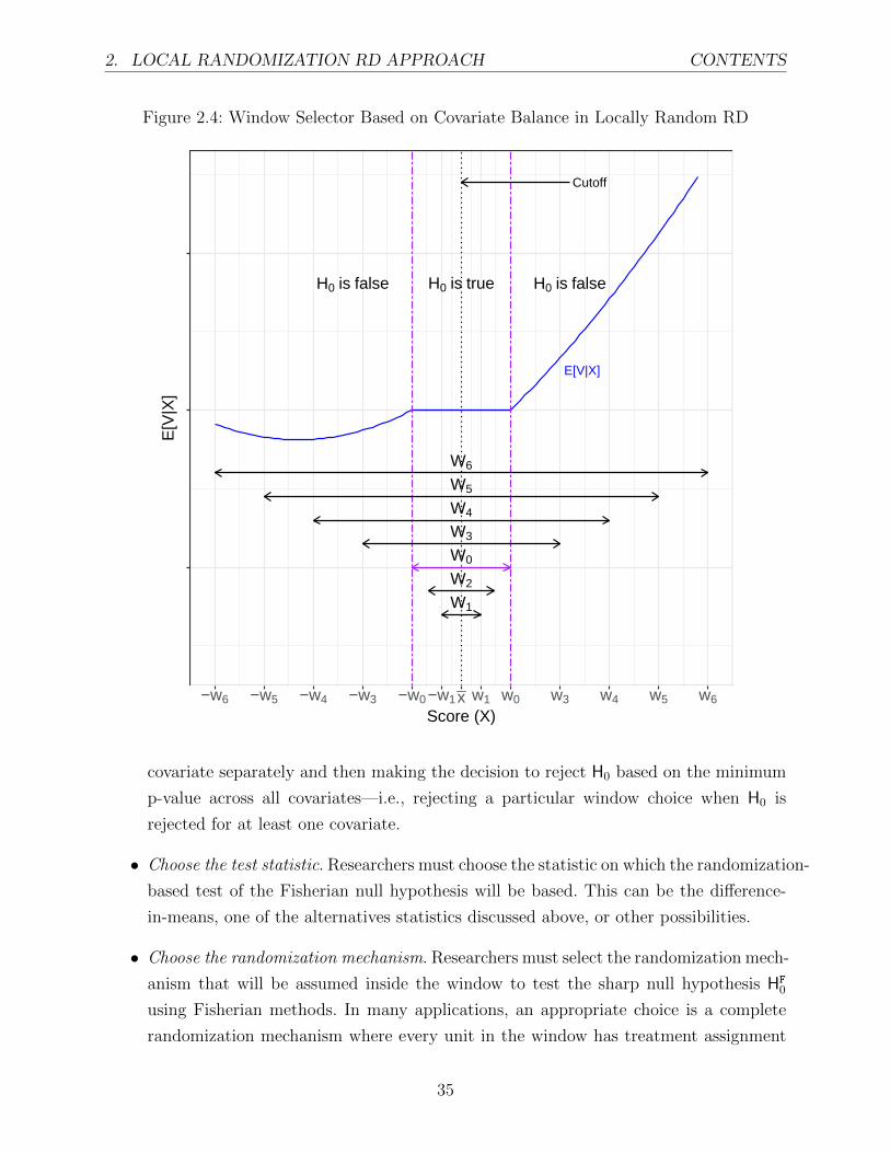
2. LOCAL RANDOMIZATION RD APPROACH CONTENTS
Figure 2.4: Window Selector Based on Covariate Balance in Locally Random RD
E[V|X]
Cutoff
W6
W5
W4
W3
W0
W2
W1
H0 is trueH0 is false H0 is false
−w6 −w5 −w4 −w3 −w0−w1x w1 w0 w3 w4 w5 w6
Score (X)
E[V
|X]
covariate separately and then making the decision to reject H0 based on the minimum
p-value across all covariates—i.e., rejecting a particular window choice when H0 is
rejected for at least one covariate.
• Choose the test statistic. Researchers must choose the statistic on which the randomization-
based test of the Fisherian null hypothesis will be based. This can be the difference-
in-means, one of the alternatives statistics discussed above, or other possibilities.
• Choose the randomization mechanism. Researchers must select the randomization mech-
anism that will be assumed inside the window to test the sharp null hypothesis HF0
using Fisherian methods. In many applications, an appropriate choice is a complete
randomization mechanism where every unit in the window has treatment assignment
35

2. LOCAL RANDOMIZATION RD APPROACH CONTENTS
probability 1/(nW0nW0,t
).
• Choose a minimum number of observations in the smallest window. In actual applica-
tions, if the smallest window around x where the null hypothesis is tested is too small,
it will contain too few observations and the test will not have enough power to reject
the null hypothesis even if it is false. Thus, researchers must ensure that the smallest
window considered contains a minimum number of observations to ensure acceptable
power; we recommend that the minimum window have at least roughly ten observations
on either side of the cutoff.
• Choose α?. The threshold significance level determines when a null hypothesis is con-
sidered rejected. Since the main concern is failing to reject a null hypothesis when it
is false—in contrast to the usual concern about rejecting a true null hypothesis—the
level of the test should be higher than conventional levels. When we test H0 at a higher
level, we tolerate a higher probability of Type I error and a lower probability of con-
cluding that the covariate is unrelated to the treatment assignment when in fact it is.
We recommend setting α? ≥ 0.15 if possible, and ideally no smaller than 0.10.
Once researchers have selected the relevant covariates, the test statistic, the randomiza-
tion mechanism in the window, and the threshold significance level α?, the window selection
procedure can be implemented with the following algorithm:
1. Start with a symmetric window of length 2wj, Wj = [x− wj, x+ wj].
2. For every covariate Zk, k = 1, 2, . . . , K, use the test statistic Tk and the chosen ran-
domization mechanism to test HF0 using a Fisherian framework. Use only observations
with scores inside Wj. Compute the associated p-value, pk. (If using an omnibus test,
compute the single omnibus p-value.)
3. Compute the minimum p-value pmin = min(p1, p2, . . . , pK). (If using an omnibus test,
set pmin to the single omnibus p-value.)
(a) If pmin > α?, do not reject the null hypothesis and increase the length of the
window by 2wstep, Wj+1 = [x − wj − wstep, x + wj + wstep]. Set Wj = Wj+1 and
go back to step (2).
(b) If pmin ≤ α?, reject the null hypothesis and conclude that the largest window
where the local randomization assumption is plausible is Wj.
36

2. LOCAL RANDOMIZATION RD APPROACH CONTENTS
To see how the procedure works in practice, we use it to select a window in the Meyers-
son application using the set of predetermined covariates described above: vshr islam1994,
partycount, lpop1994, i89, merkezi, merkezp, subbuyuk, buyuk. We use the function
rdwinselect, which is one of the functions in the rdlocrand library or package. The main
arguments are the score variable X, the matrix of predetermined covariates, and the sequence
of nested windows; for simplicity, only symmetric windows are considered. We also choose
1,000 simulations for the calculation of Fisherian p-values in each window.
There are two ways to increment the length of the windows in rdwinselect. One is to
increment the length of the window in fixed steps, which can be implemented with the option
wstep. For example, if the first window selected is [0.1, 0.1] and wstep = 0.1, the sequence
is W1 = [0.1, 0.1],W2 = [0.2, 0.2], W3 = [0.3, 0.3], etc. The other is to increase the length
of the window so that the number of observations increases by a minimum fixed amount
on every step, which can be done via the option wobs. For example, by setting wobs = 2,
every window in the sequence is the smallest symmetric window such that the number of
added observations on each side of the cutoff relative to the prior window is at least 2.
By default, rdwinselect starts with the smallest window that has at least 10 observations
on either side, but this default behavior can be changed with the options wmin or obsmin.
Finally, rdwinselect uses the chosen level α? to recommend the chosen window; the default
is α? = 0.15, but this can be modified with the level option.
We start by considering a sequence of symmetric windows where we increase the length
in every step by the minimum amount so that we add at least 2 observations on either side
in each step. We achieve this by setting wobs=2.
> Z = cbind(data$i89 , data$vshr_islam1994 , data$partycount , data$lpop1994 ,
+ data$merkezi , data$merkezp , data$subbuyuk , data$buyuk)
> colnames(Z) = c("i89", "vshr_islam1994", "partycount", "lpop1994",
+ "merkezi", "merkezp", "subbuyuk", "buyuk")
> out = rdwinselect(X, Z, seed = 50, reps = 1000, wobs = 2)
Window selection for RD under local randomization
Number of obs = 2629
Order of poly = 0
Kernel type = uniform
Reps = 1000
Testing method = rdrandinf
Balance test = diffmeans
Cutoff c = 0 Left of c Right of c
Number of obs 2314 315
1st percentile 24 3
37

2. LOCAL RANDOMIZATION RD APPROACH CONTENTS
5th percentile 115 15
10th percentile 231 31
20th percentile 463 62
Window length / 2 p-value Var. name Bin.test Obs <c
Obs >=c
0.446 0.451 i89 1 9
10
0.486 0.209 i89 1 11
12
0.536 0.253 i89 1 12
13
0.699 0.238 i89 0.585 13
17
0.856 0.27 i89 0.377 13
19
0.944 0.241 i89 0.627 17
21
1.116 0.048 i89 0.28 17
25
1.274 0.059 i89 0.371 19
26
1.343 0.352 merkezi 0.312 20
28
1.42 0.365 i89 0.272 22
31
Recommended window is [ -0.944;0.944] with 38 observations (17 below , 21
above).
Analogous Stata command
. global covs "i89 vshr_islam1994 partycount lpop1994 merkezi merkezp subbuyuk buyuk"
. rdwinselect X $covs, seed(50) wobs(2)
The top and middle panels in the rdwinselect output are very similar to the corre-
sponding panels in the rdrandinf output. One difference is the Testing method, which
indicates whether randomization-based methods are used to test HF0, or Normal approxima-
tions methods are used to test HN0. The default is randomization-based methods, but this can
be changed with the approximate option. The other difference in the output is the Balance
test, which indicates the type of test statistic used for testing the null hypothesis—the
default is diffmeans, the difference-in-means. The option statistic allows the user to
select a different test statistic; the available options are the Kolmogorov-Smirnov statistic
(ksmirnov), the Wilcoxon-Mann-Whitney studentized statistic (ranksum), and Hotelling’s
T-squared statistic (hotelling).
38

2. LOCAL RANDOMIZATION RD APPROACH CONTENTS
The bottom panel shows tests of the null hypothesis for each window considered. By
default, rdwinselect starts with the smallest symmetric window that has at least 10 obser-
vations on either side of the cutoff. Since we set wobs=2, we continue to consider the smallest
possible (symmetric) windows so that at least 2 observations are added on each side of the
cutoff in every step. For every window, the column p-value reports pmin—the minimum of
the p-values associated with the K tests of the null hypothesis of no effect performed for each
of the K covariates, or the unique p-value if an omnibus test is used. The column Var. name
reports the covariate associated with the minimum p-value—that is, the covariate Zk such
that pk = pmin.
Finally, the column Bin. test uses a Binomial test to calculate the probability of ob-
serving nW,+ successes out of nW trials, where nW,t is the number of observations within the
window that are above the cutoff (reported in column Obs>c) and nW is the total number of
observations within the window (which can be calculated by adding the number reported in
columns Obs<c and Obs>c). We postpone discussion of this test until the upcoming section
on falsification of RD designs under a local randomization framework.
The output indicates that the p-values are above 0.20 in all windows between the mini-
mum window [−0.446, 0.446] and [−0.944, 0.944]. In the window immediately after [−0.944, 0.944],
the p-value drops to 0.048, considerably below the suggested 0.15 threshold. The data-driven
window is therefore W ? = [−0.944, 0.944]. After this window, the p-values start decreasing,
albeit initially this decrease is not necessarily monotonic. By default, rdwinselect only
shows the first 20 windows; in order to see the sharp decrease in p-values that occurs as
larger windows are considered, we set the option nwindows=50 to see the output of the first
50 windows. We also set the option plot=TRUE, to create a plot of the minimum p-values
associated with the length of each window considered—the plot is shown in Figure 2.5 below.
> Z = cbind(data$i89 , data$vshr_islam1994 , data$partycount , data$lpop1994 ,
+ data$merkezi , data$merkezp , data$subbuyuk , data$buyuk)
> colnames(Z) = c("i89", "vshr_islam1994", "partycount", "lpop1994",
+ "merkezi", "merkezp", "subbuyuk", "buyuk")
> out = rdwinselect(X, Z, seed = 50, reps = 1000, wobs = 2, nwindows = 50,
+ plot = TRUE)
Window selection for RD under local randomization
Number of obs = 2629
Order of poly = 0
Kernel type = uniform
Reps = 1000
Testing method = rdrandinf
Balance test = diffmeans
39

2. LOCAL RANDOMIZATION RD APPROACH CONTENTS
Cutoff c = 0 Left of c Right of c
Number of obs 2314 315
1st percentile 24 3
5th percentile 115 15
10th percentile 231 31
20th percentile 463 62
Window length / 2 p-value Var. name Bin.test Obs <c
Obs >=c
0.446 0.451 i89 1 9
10
0.486 0.209 i89 1 11
12
0.536 0.253 i89 1 12
13
0.699 0.238 i89 0.585 13
17
0.856 0.27 i89 0.377 13
19
0.944 0.241 i89 0.627 17
21
1.116 0.048 i89 0.28 17
25
1.274 0.059 i89 0.371 19
26
1.343 0.352 merkezi 0.312 20
28
1.42 0.365 i89 0.272 22
31
1.49 0.171 merkezi 0.229 23
33
1.556 0.31 merkezi 0.245 25
35
1.641 0.188 merkezi 0.26 27
37
1.858 0.206 merkezi 0.328 29
38
1.914 0.244 merkezi 0.403 31
39
2.019 0.26 merkezi 0.416 33
41
2.097 0.211 vshr_islam1994 0.653 37
42
2.158 0.096 vshr_islam1994 0.657 38
43
2.319 0.048 vshr_islam1994 1 44
45
2.433 0.016 vshr_islam1994 0.839 50
47
2.583 0.008 vshr_islam1994 0.842 52
49
2.643 0.006 vshr_islam1994 0.922 53
40

2. LOCAL RANDOMIZATION RD APPROACH CONTENTS
51
2.746 0.002 vshr_islam1994 1 54
54
3.009 0.002 vshr_islam1994 1 56
56
3.051 0.005 vshr_islam1994 1 58
58
3.094 0.001 vshr_islam1994 0.928 62
60
3.178 0 vshr_islam1994 0.929 64
62
3.462 0 vshr_islam1994 0.491 72
63
3.595 0 vshr_islam1994 0.444 74
64
3.704 0 vshr_islam1994 0.356 77
65
3.821 0 vshr_islam1994 0.251 82
67
3.963 0 vshr_islam1994 0.258 84
69
4.181 0 vshr_islam1994 0.153 89
70
4.287 0 vshr_islam1994 0.138 92
72
4.417 0 vshr_islam1994 0.192 94
76
4.488 0.001 vshr_islam1994 0.168 95
76
4.585 0 vshr_islam1994 0.113 99
77
4.719 0 vshr_islam1994 0.1 101
78
4.899 0 vshr_islam1994 0.067 106
80
5.03 0 vshr_islam1994 0.095 107
83
5.2 0 vshr_islam1994 0.098 109
85
5.346 0 vshr_islam1994 0.089 112
87
5.421 0 vshr_islam1994 0.078 114
88
5.482 0 vshr_islam1994 0.092 114
89
5.593 0 vshr_islam1994 0.081 116
90
5.676 0 vshr_islam1994 0.073 119
92
5.779 0 vshr_islam1994 0.075 120
93
5.878 0 vshr_islam1994 0.119 121
97
6.039 0 vshr_islam1994 0.053 128
41

2. LOCAL RANDOMIZATION RD APPROACH CONTENTS
98
6.266 0 vshr_islam1994 0.034 131
98
Recommended window is [ -0.944;0.944] with 38 observations (17 below , 21
above).
Analogous Stata command
. global covs "i89 vshr_islam1994 partycount lpop1994 merkezi merkezp subbuyuk buyuk"
. rdwinselect X $covs, seed(50) wobs(2) nwindows(50) plot
Figure 2.5: Window selection: minimum P-value against window length—Meyersson data
●
●
●
●
●
●
●●
●
●
●
●
●
●
●
●
●
●
●
●●●● ●●●● ● ● ● ● ● ● ● ●●● ● ● ● ● ●●● ●●●● ● ●
1 2 3 4 5 6
0.0
0.1
0.2
0.3
0.4
window.list
Pva
ls
The plot in Figure 2.5 shows that, in the sequence of windows considered, the minimum
p-value is above 0.20 for all windows smaller than [-1,1], and decreases below 0.1 as the
windows get larger than [-1,1]. Although the p-values increase again for windows between
[-1,1] and [-2,2], they decrease sharply once windows larger than [-2,2] are considered. The
pattern in this plot is common in most applications: a strong negative relationship between p-
values and window length, with high p-values for the smallest windows that decrease rapidly
and stay at zero once the window length is larger than some threshold. Note that in this
empirical example, the absolute value of the running variable (Islamic margin of victory),
ranges from 0 to 100. Yet the p-values become approximately zero for any window larger
42

2. LOCAL RANDOMIZATION RD APPROACH CONTENTS
than [−3, 3], suggesting that there are sharp differences between municipalities where the
Islamic party wins and municipalities where it loses, even when the election is decided by
moderate margins. This shows that, the local randomization, if it holds at all, will hold in a
small window near the cutoff.
If we want to choose the window using a sequence of symmetric windows of fixed length
rather than controlling the minimum number of observations, we use the wstep option.
Calling rdwinselect with wstep=0.1 performs the covariate balance tests in a sequence of
windows that starts at the minimum window and increases the length by 0.1 at each side of
the cutoff.
> Z = cbind(data$i89 , data$vshr_islam1994 , data$partycount , data$lpop1994 ,
+ data$merkezi , data$merkezp , data$subbuyuk , data$buyuk)
> colnames(Z) = c("i89", "vshr_islam1994", "partycount", "lpop1994",
+ "merkezi", "merkezp", "subbuyuk", "buyuk")
> out = rdwinselect(X, Z, seed = 50, reps = 1000, wstep = 0.1,
+ nwindows = 25)
Window selection for RD under local randomization
Number of obs = 2629
Order of poly = 0
Kernel type = uniform
Reps = 1000
Testing method = rdrandinf
Balance test = diffmeans
Cutoff c = 0 Left of c Right of c
Number of obs 2314 315
1st percentile 24 3
5th percentile 115 15
10th percentile 231 31
20th percentile 463 62
Window length / 2 p-value Var. name Bin.test Obs <c
Obs >=c
0.446 0.451 i89 1 9
10
0.546 0.241 i89 1 12
13
0.646 0.22 i89 0.851 13
15
0.746 0.241 i89 0.473 13
18
0.846 0.243 i89 0.377 13
19
0.946 0.234 i89 0.627 17
21
43

2. LOCAL RANDOMIZATION RD APPROACH CONTENTS
1.046 0.061 i89 0.349 17
24
1.146 0.069 i89 0.28 17
25
1.246 0.057 i89 0.451 19
25
1.346 0.366 merkezi 0.312 20
28
1.446 0.254 merkezi 0.22 22
32
1.546 0.24 i89 0.298 25
34
1.646 0.187 merkezi 0.26 27
37
1.746 0.198 merkezi 0.215 27
38
1.846 0.224 i89 0.268 28
38
1.946 0.242 merkezi 0.477 32
39
2.046 0.259 merkezi 0.567 35
41
2.146 0.095 vshr_islam1994 0.657 38
43
2.246 0.066 vshr_islam1994 0.914 42
44
2.346 0.056 vshr_islam1994 1 45
45
2.446 0.012 vshr_islam1994 0.839 50
47
2.546 0.011 vshr_islam1994 0.841 51
48
2.646 0.006 vshr_islam1994 0.922 53
51
2.746 0 vshr_islam1994 1 53
54
2.846 0.003 vshr_islam1994 1 55
55
Recommended window is [ -0.946;0.946] with 38 observations (17 below , 21
above).
Analogous Stata command
. global covs "i89 vshr_islam1994 partycount lpop1994 merkezi merkezp subbuyuk buyuk"
. rdwinselect X $covs, seed(50) wstep(0.1) nwindows(25)
The suggested window is [−0.946, 0.946], very similar to the [−0.944, 0.944] window cho-
sen above with the wobs=2 option.
We can now use rdrandinf to perform a local randomization analysis in the chosen
44

2. LOCAL RANDOMIZATION RD APPROACH CONTENTS
window. For this, we use the options wl and wr to input, respectively, the lower and upper
limit of the chosen window W ? = [−0.944, 0.944]. We also use the option d = 3.020 to
calculate the power of a Neyman test to reject the null hypothesis of null average treatment
effect when the true average difference is 3.020. This value is the continuity-based linear
polynomial point estimate reproduced above (and discussed extensively in Part I).
The difference-in-means in the chosen window W ? = [−0.944, 0.944] is 2.638, considerably
similar to the continuity-based local linear point estimate of 3.020. However, using a Neyman
approach, we cannot distinguish this average difference from zero, with a p-value of 0.333.
Similarly, we fail to reject the Fisherian sharp null hypothesis that an electoral victory by
the Islamic party has no effect on the female education share for any municipality (p-value
0.386). As shown in the last column, the large-sample power to detect a difference of around
3 percentage points is only 19.4%. Naturally, the small number of observations in the chosen
window (23 and 27 below and above the cutoff, respectively) limits statistical power. In
addition, the effect of 2.638, although much larger than the 1.072 estimated in the ad-hoc [-
2.5, 2.5] window, is still a small effect, as it is less than a third of one standard deviation of the
female education share in the control group—we see this by calculating 2.638/8.615 = 0.306.
In accordance with these results, the Fisherian 95% confidence interval under a constant
treatment effect model is [−2.8 , 8.5], consistent with both positive and negative effects.
> ci_vec = c(0.05, seq(from = -10, to = 10, by = 0.1))
> out = rdrandinf(Y, X, wl = -0.944, wr = 0.944, seed = 50, reps = 1000,
+ ci = ci_vec)
Selected window = [ -0.944;0.944]
Running randomization -based test ...
Randomization -based test complete.
Running sensitivity analysis ...
Sensitivity analysis complete.
Number of obs = 2629
Order of poly = 0
Kernel type = uniform
Reps = 1000
Window = set by user
H0: tau = 0
Randomization = fixed margins
Cutoff c = 0 Left of c Right of c
Number of obs 2314 315
45

2. LOCAL RANDOMIZATION RD APPROACH CONTENTS
Eff. number of obs 23 27
Mean of outcome 13.579 16.217
S.d. of outcome 8.615 10.641
Window -0.944 0.944
Finite sample Large sample
Statistic T P>|T| P>|T| Power vs d =
4.307
Diff. in means 2.638 0.386 0.333 0.353
95% confidence interval: [ -2.8 ,8.5]
Analogous Stata command
. rdrandinf Y X, wl(-0.944) wr(0.944) seed(50) ci(0.05 -10(0.1)10)
Finally, we mention that instead of calling rdwinselect first and rdrandinf second, we
can choose the window and perform inference in one step by using the covariates option
in rdrandinf.
> Z = cbind(data$i89 , data$vshr_islam1994 , data$partycount , data$lpop1994 ,
+ data$merkezi , data$merkezp , data$subbuyuk , data$buyuk)
> colnames(Z) = c("i89", "vshr_islam1994", "partycount", "lpop1994",
+ "merkezi", "merkezp", "subbuyuk", "buyuk")
> out = rdrandinf(Y, X, covariates = Z, seed = 50, d = 3.019522)
Running rdwinselect ...
rdwinselect complete.
Selected window = [ -0.917068123817444;0.917068123817444]
Running randomization -based test ...
Randomization -based test complete.
Number of obs = 2629
Order of poly = 0
Kernel type = uniform
Reps = 1000
Window = rdwinselect
H0: tau = 0
Randomization = fixed margins
Cutoff c = 0 Left of c Right of c
Number of obs 2314 315
Eff. number of obs 22 27
46

2. LOCAL RANDOMIZATION RD APPROACH CONTENTS
Mean of outcome 13.266 16.217
S.d. of outcome 8.682 10.641
Window -0.917 0.917
Finite sample Large sample
Statistic T P>|T| P>|T| Power vs d =
3.02
Diff. in means 2.952 0.301 0.285 0.194
Analogous Stata command
. global covs "i89 vshr_islam1994 partycount lpop1994 merkezi merkezp subbuyuk buyuk"
. rdrandinf Y X, covariates($covs) seed(50) d(3.019522)
However, it is usually better to first choose the window using rdwinselect and then
use rdrandinf. The reason is that calling rdwinselect by itself will never show outcome
results, and will reduce the possibility of choosing the window where the outcome results are
in the “expected” direction—in other words, choosing the window without looking at the
outcome results minimizes pre-testing and specification-searching issues.
2.4 Falsification Analysis In The Local Randomization Approach
In Part I, we discussed the importance of conducting falsification tests to provide evidence in
support of the RD assumptions. Falsification and validation analyses are as important in the
local randomization framework as they are in the continuity-based framework. The difference
resides in their implementation. Instead of providing empirical evidence in favor of continuity
assumptions as in the continuity-based approach, the main goal in a local randomization
approach is to provide evidence consistent with the local randomization assumption. Thus,
the methods employed to perform a falsification analysis in the local randomization approach
must be different.
We now discuss four types of empirical falsification tests for a local randomization RD
design, all of which we discussed in our companion Part I monograph in the context of the
continuity-based approach: (i) tests of a null treatment effect on pre-treatment covariates or
placebo outcomes, (ii) tests to assess the density of the score around the cutoff, (iii) treatment
effect estimation at artificial cutoffs values, and (v) sensitivity to neighborhood choices. We
now discuss and illustrate how to implement these tests in the local randomization approach.
In Part I, we also discussed an additional falsification test based on an analysis that excludes
the observations that are closest to the cutoff, an idea sometimes referred to as the “donut
47

2. LOCAL RANDOMIZATION RD APPROACH CONTENTS
hole” test. This test is most natural in a continuity-based approach, where one is interested
in knowing whether the extrapolation is heavily influenced by the few observations closest to
the cutoff and the analysis typically contains at least hundreds of observations. In contrast, in
a local randomization approach, the chosen window is likely to be very small, and removing
the observations closest to the cutoff may result in too few observations and render the
analysis unfeasible. For this reason, we omit this method from our discussion.
2.4.1 Predetermined Covariates and Placebo Outcomes
This crucial falsification test focuses on two types of variables: predetermined covariates—
variables that are determined before the treatment is assigned, and placebo outcomes—
variables that are determined after the treatment is assigned but for which we have scientific
reasons to believe that they are unaffected by the treatment. The idea is that, in a valid
RD design, there should be no systematic differences between treated and control groups at
the cutoff in terms of both placebo outcomes and predetermined covariates, because these
variables could not have been affected by the treatment. For implementation, the researcher
conducts a test of the hypothesis that the treatment effect is zero for each predetermined
covariate and placebo outcome. If the treatment does have an effect on these variables, the
plausibility of the RD assumptions is called into question.
An important principle behind this type of falsification analysis is that all predetermined
covariates and placebo outcomes should be analyzed in the same way as the outcome of inter-
est. In the local randomization approach, this means that the null hypothesis of no treatment
effect should be tested within the window where the assumption of local randomization is
assumed to hold, using the same inference procedures and the same treatment assignment
mechanism and test statistic used for the analysis of the outcome of interest. Since in this
approach W0 is the window where the treatment is assumed to have been randomly assigned,
all covariates and placebo outcomes should be analyzed within this window. This illustrates
a fundamental difference between the continuity-based and the randomization-based ap-
proach: in the former, estimation and inference requires approximating unknown regression
functions, which requires estimating separate bandwidths for each variable analyzed; in the
latter, since the treatment is assumed to be as-if-randomly assigned in W0, all analysis occur
within the same window, W0.
In our analysis above we chose the windowW0 = [−0.944, 0.944] for the local-randomization
approach. In order to test if the predetermined covariates are balanced within this window,
we analyze their behavior in this window on each side of the cutoff using randomization
48

2. LOCAL RANDOMIZATION RD APPROACH CONTENTS
inference techniques. We use the difference-in-means statistic, the same statistic we used for
the outcome of interest. Under the local randomization assumption, we expect the difference-
in-means between treated and control groups for each covariate to be indistinguishable from
zero within W0. Naturally, we already know that the covariates that we used to choose the
window are balanced in the chosen window. In this sense, the window selector procedure is
itself a validation procedure. We note, however, that it is possible (and indeed common) for
researchers to choose the window based on a given set of covariates, and then assess balance
on a different set.
In order to test this formally, we use the rdrandinf function, using each covariate as
the outcome of interest. For example, when we study the covariate vshr islam1994, we see
that the difference-in-means statistic is very small (0.328 − 0.319 = −0.009), and the finite
sample p-value is large (0.689). That is, this covariate is balanced inside W0 according to
this test-statistic.
> out = rdrandinf(data$vshr_islam1994 , X, seed = 50, wl = -0.944,
+ wr = 0.944)
Selected window = [ -0.944;0.944]
Running randomization -based test ...
Randomization -based test complete.
Number of obs = 2629
Order of poly = 0
Kernel type = uniform
Reps = 1000
Window = set by user
H0: tau = 0
Randomization = fixed margins
Cutoff c = 0 Left of c Right of c
Number of obs 2314 315
Eff. number of obs 23 27
Mean of outcome 32.816 31.872
S.d. of outcome 9.41 8.141
Window -0.944 0.944
Finite sample Large sample
Statistic T P>|T| P>|T| Power vs d =
4.705
Diff. in means -0.944 0.702 0.707 0.466
49

2. LOCAL RANDOMIZATION RD APPROACH CONTENTS
Analogous Stata command
. rdrandinf vshr_islam1994 X, wl(-.944) wr(.944)
Table 2.3: Formal Local-Randomization Analysis for Covariates
VariableMean of Mean of Diff-in-Means Fisherian Number ofControls Treated Statistic p-value Observations
Percentage of men aged 15-20 with high school education 19.219 21.742 2.523 0.275 50Islamic Mayor in 1989 0.000 0.150 0.150 0.222 37Islamic percentage of votes in 1994 32.816 31.872 -0.944 0.712 50Number of parties receiving votes 1994 6.348 6.074 -0.274 0.794 50Log population in 1994 8.566 8.594 0.028 0.954 50District center 0.609 0.519 -0.090 0.595 50Province center 0.087 0.037 -0.050 0.580 50Sub-metro center 0.087 0.074 -0.013 1.000 50Metro center 0.043 0.037 -0.006 1.000 50
Table 2.3 contains a summary of this analysis for all covariates using randomization
inference. We cannot conclude that the control and treatment means are different for any
covariate, since the p-values are above 0.15 in all cases. There is no statistical evidence
of imbalance (in terms of their means) inside of this window. Note that the number of
observations is fixed in all cases. This happens because the window in which we analyze
these covariates is not changing, is always W0, whereas in the continuity-based approach the
MSE-optimal bandwidth depends on the particular outcome being used, and therefore the
number of observations is different for every covariate.
This analysis can also be carried out visually, by using rdplot restricted to W0, with
p = 0 and a uniform kernel. If the window was chosen appropriately, then all covariates
should have similar means above and below the cutoff. For example, we can construct an
RD plot with these characteristics for the covariate vshr islam1994.
> rdplot(data$vshr_islam1994[abs(X) <= 0.944] , X[abs(X) <= 0.944] ,
+ p = 0, kernel = "uniform", x.label = "Score", y.label = "",
+ title = "", x.lim = c(-1.25, 1.25) , y.lim = c(0.2, 0.45))
Analogous Stata command
. rdplot vshr_islam1994 X if abs(X) <= .944, h(.944) p(0) kernel(uniform)
50

2. LOCAL RANDOMIZATION RD APPROACH CONTENTS
●
●
●
●
●
●
●
●
−1.0 −0.5 0.0 0.5 1.0
2426
2830
3234
36
Score
Figure 2.6 contains analogous RD plots for the six predetermined covariates analyzed
above. In most cases, the visual inspection shows that the means of these covariates seem to
be similar on each side of the cutoff, consistent with the results from the window selection
procedure discussed in Section 2 and the formal analysis in Table 2.3.
51

2. LOCAL RANDOMIZATION RD APPROACH CONTENTS
Figure 2.6: Illustration of Local Randomization RD Effects on Covariates—Meyersson Data
●
●
●
●
●
●
●
−1.0 −0.5 0.0 0.5 1.0
8.0
8.2
8.4
8.6
8.8
9.0
9.2
Score
(a) Log Population in 1994
●
●
●
●
●
●
●
−1.0 −0.5 0.0 0.5 1.0
4.5
5.0
5.5
6.0
6.5
7.0
7.5
8.0
Score
(b) Number of Parties Receiving Votes in 1994
●
●
●
●
●
●
●
●
−1.0 −0.5 0.0 0.5 1.0
2426
2830
3234
36
Score
(c) Islamic Vote Share in 1994
●
●
●
●
●
−1.0 −0.5 0.0 0.5 1.0
0.00
0.05
0.10
0.15
0.20
0.25
Score
(d) Islamic Mayor in 1989
●
●
●
● ● ●
●
−1.0 −0.5 0.0 0.5 1.0
0.50
0.55
0.60
0.65
0.70
0.75
0.80
Score
(e) District center indicator
●
● ●
●
● ● ● ● ●
●
● ● ● ● ●
−1.0 −0.5 0.0 0.5 1.0
0.00
0.05
0.10
0.15
0.20
0.25
0.30
Score
(f) Province center indicator52

2. LOCAL RANDOMIZATION RD APPROACH CONTENTS
2.4.2 Density of Running Variable
Another important falsification test, already discussed in Part I, is a density test that analyzes
whether the number of observations just above the cutoff is roughly similar to the number of
observations just below the cutoff. The idea is that, if units lack the ability to control precisely
the value of the score they receive, they should be as likely to receive a score value just above
the cutoff as they are to receive a score value just below it. In a local randomization approach,
this falsification analysis is implemented by testing the null hypothesis that, within the
window W0 where the treatment is assumed to be randomly assigned, the number of treated
and control observations is consistent with whatever assignment mechanism is assumed inside
W0.
For example, assuming a simple “coin flip” or Bernoulli trial with probability of success q,
we would expect that the control sample size, nW0,−, and treatment sample size, nW0,+, within
W0 to be compatible with the numbers generated by these nW0,− + nW0,+ = nW0 Bernoulli
trials. In this case, the number of treated units in W0 follows a binomial distribution, and the
null hypothesis of the test is that the probability of success in the nW0 Bernoulli experiments
is q. As discussed, the true probability of treatment is unknown. In practice, researchers can
choose q = 1/2 (a choice that can be justified from a large sample perspective when the score
is continuous), or can set the value of q equal to the observed proportion of treated units in
the window.
The binomial test is implemented in all common statistical software, and is also part
of the rdlocrand package via the rdwinselect command. Using the Meyersson data, we
can implement this falsifcation test in our selected window W0 = [−0.944, 0.944] employing
rdwinselect using the score as the single argument. Since we only want to see the binomial
test in this window, we use the option nwindows(1).
> out = rdwinselect(X, wmin = 0.944, nwindows = 1)
Window selection for RD under local randomization
Number of obs = 2629
Order of poly = 0
Kernel type = uniform
Reps = 1000
Testing method = rdrandinf
Balance test = diffmeans
Cutoff c = 0 Left of c Right of c
Number of obs 2314 315
1st percentile 24 3
53

2. LOCAL RANDOMIZATION RD APPROACH CONTENTS
5th percentile 115 15
10th percentile 231 31
20th percentile 463 62
Window length / 2 p-value Var. name Bin.test Obs <c
Obs >=c
0.944 NA NA 0.672 23
27
Analogous Stata command
. rdwinselect X, wmin(0.944) nwindows(1)
There are 23 control observations and 27 treated observations in the window. The column
Bin. test shows the p-value of a binomial test that uses a success probability equal to 1/2.
The p-value is 0.672, so we find no evidence of “sorting” around the cutoff in the window
W0 = [−0.944, 0.944]—the difference in the number of treated and control observations in
this window is entirely consistent with what would be expected if municipalities were assigned
to an Islamic win or loss by the flip of an unbiased coin. This is expected, as the observed
share of treated observations in the window, 2723+27
= 0.54, is very close to 1/2.
We can also implement the binomial test using q = 1/2. For this, we can simply use the
base distribution in R or Stata.
> binom.test(27, 50, 1/2)
Exact binomial test
data: 27 and 50
number of successes = 27, number of trials = 50, p-value = 0.6718
alternative hypothesis: true probability of success is not equal to 0.5
95 percent confidence interval:
0.3932420 0.6818508
sample estimates:
probability of success
0.54
Analogous Stata command
. bitesti 50 27 1/2
As expected, the two-sided p-value is 0.6718, which is equal (after rounding) to the p-
value obtained using rdwinselect.
54

2. LOCAL RANDOMIZATION RD APPROACH CONTENTS
2.4.3 Placebo Cutoffs
This falsfication test chooses one ore more artificial or “fake” cutoff values at which the
probability of treatment assignment does not change, and analyzes the outcome of interest
at these artificial cutoffs using the same methods used to conduct the analysis at the actual
cutoff. The expectation is that no effect should be found at any of the artificial cutoffs. To
avoid contamination from the actual treatment effect, only treated observations are included
for fake cutoffs above the actual cutoff, and only control observations are included for cutoffs
below the actual cutoff.
In the local-randomization approach, one possible implementation is to choose several
artificial cutoff values, and then conduct a randomization-based analysis of the outcome
using a symmetric window of the same length as the original window W0 around each of the
fake cutoffs. Since our chosen window in the Meyersson application is W0 = [−0.944, 0.944],
we consider windows of length ±0.944 around each artificial cutoff. For example, for the
cutoff 2, we analyze the outcome in the window [1.056, 2.944].
2.4.4 Sensitivity to Window Choice
Just like in a continuity-based approach researchers are interested in the sensitivity of the
results to the bandwidth choice, in a local randomization approach we are often interested
in sensitivity to the window choice. To assess sensitivity to window choice, researchers can
simply consider windows smaller than W0 and repeat the randomization-based analysis for
the outcome of interest as conducted in the original window—that is, using the same test-
statistic, same randomization mechanism, etc. This analysis should be implemented carefully,
however. If the window W0 was chosen based on covariate balance as we recommend, results
in windows larger than W0 will not be reliable because in such windows the treated and
control groups will be imbalanced in important covariates. Thus, the sensitivity analysis
should only consider windows smaller than W0; unfortunately, in many applications this
analysis will be limited by the small number observations that is likely to occur in these
windows. In the Meyersson application, our chosen window is W0 = [−0.944, 0.944], and
has 23 and 27 observations on either side of the cutoff. We consider the smaller windows
W0 = [−0.85, 0.85], W0 = [−0.75, 0.75], and W0 = [−0.75, 0.75] below.
55

2. LOCAL RANDOMIZATION RD APPROACH CONTENTS
2.5 When To Use The Local Randomization Approach
Unlike an experiment, the RD treatment assignment rule does not imply that the treatment
is randomly assigned within some window. Like the continuity assumption, the local ran-
domization assumption must be made in addition to the RD assignment mechanism, and
is not directly testable. But the local randomization assumption is strictly stronger than
the continuity assumption, in the sense that if there is a window around x in which the
regression functions are constant functions of the score, these regression functions will also
be continuous functions of the score at x—but the converse is not true. Why, then, would
researchers want to impose stronger assumptions to make their inferences?
It is useful to remember that the local-polynomial approach, although based on the weaker
condition of continuity, relies on extrapolation because there are no observations exactly
at the cutoff. The continuity assumption does not imply a specific functional form of the
regression functions near the cutoff, as it approximates these functions using non-parametric
methods; however, this approximation relies on extrapolation methods and introduces an
approximation erorr that is only negligible if the sample size is large enough. This makes the
continuity-based approach more appealing if there are enough observations near the cutoff
to approximate the regression functions with reasonable accuracy—but possibly inadequate
when the number of observations is small. In applications with few observations, the local
randomization approach has the advantage of requiring minimal extrapolation and avoiding
the use of smoothing methods.
Another situation in which a local randomization approach may be preferable to a
continuity-based approach is when the running variable is discrete—i.e., when multiple units
share the same value of the score, as the continuity-based approach is not directly applicable
in this case. We consider this issue in the next section, where we discuss how to analyze RD
designs with discrete running variables.
2.6 Further Readings
Textbook reviews of Fisherian and Neyman estimation and inference methods in the context
of analysis of experiments are given by Rosenbaum (2002, 2010) and Imbens and Rubin
(2015); the latter also discusses super-population approaches and their connections to fi-
nite population inference methods. Ernst (2004) discusses the connection and distinctions
between randomization and permutation inference methods. Cattaneo et al. (2015) propose
Fisherian randomization-based inference to analyze RD designs based on a local random-
56

2. LOCAL RANDOMIZATION RD APPROACH CONTENTS
ization assumption, and the window selection procedure based on covariate balance tests.
Cattaneo et al. (2017) relax the local randomization assumption to allow for a weaker exclu-
sion restriction, and also compare RD analysis in continuity-based and randomization-based
approaches. The interpretation of the RD design as a local experiment and its connection to
the continuity-based framework is also discussed by Sekhon and Titiunik (2016, 2017).
Regarding falsification analysis, Frandsen (2017) discusses a manipulation test for cases
where the score is discrete. The importance of falsification tests and the use of placebo
outcomes is discussed in general in the literature on analysis of experiments (e.g., Rosenbaum,
2002, 2010; Imbens and Rubin, 2015). Lee (2008) applies and further develops these ideas
in the RD design context, and Canay and Kamat (2018) develops a permutation inference
approach for RD designs. Ganong and Jager (2018) propose a permutation inference approach
based on the idea of placebo RD cutoffs for the Kink RD designs, Regression Kink designs,
and related settings. Falsification testing based on donut hole specifications are discussed in
Bajari et al. (2011) and Barreca et al. (2016).
57

3. RD DESIGNS WITH DISCRETE RUNNING VARIABLES CONTENTS
3 RD Designs with Discrete Running Variables
The canonical continuity-based RD design assumes that the score that determines treatment
is a continuous random variable. A random variable is continuous when the set of values
that it can take contains an uncountable number of elements. For example, a share such as
a party’s proportion of the vote is continuous, because it can take any value in the [0, 1]
interval. In practical terms, when a variable is continuous, all the observations in the dataset
have distinct values—i.e., there are no ties. In contrast, a discrete random variable such as
date of birth can only take a finite number of values; as a result, a random sample of a discrete
variable will contain “mass points”—that is, values that are shared by many observations.
When the RD score is not a continuous random variable, the local polynomial methods we
described in Part I are not directly applicable. This is a practically relevant issue, because
many real RD applications have a discrete score that can only take a finite number of
values. We now consider an empirical RD example where the running variable has mass
points in order to illustrate some of the strategies that can be used to analyze RD designs
with a discrete running variable. We employ this empirical application to illustrate how
identification, estimation, and inference can be modified when the dataset contains multiple
observations per value of the running variable.
The key issue when deciding how to analyze a RD design with a discrete score is the
number of distinct mass points. Local polynomial methods will behave essentially as if each
mass point is a single observation. Thus, if the score is discrete but the number of mass points
is sufficiently large, using local polynomial methods may still be appropriate. In contrast,
if the number of mass points is very small, local polynomial methods will not be directly
applicable. In this case, analyzing the RD design using the local randomization approach
is a natural alternative. When the score is discrete, the local randomization approach has
the advantage of that the window selection procedure is no longer needed, as the smallest
window is well defined. Regardless of the estimation and inference method employed, issues
of interpretability and extrapolation will naturally arise. In this section, we discuss and
illustrate all these issues using an example from the education literature.
3.1 The Effect of Academic Probation on Future Academic Achieve-
ment
The example we re-analyze is the study by Lindo, Sanders and Oreopoulos (2010, LSO
hereafter), who use an RD design to investigate the impact of placing students on academic
58

3. RD DESIGNS WITH DISCRETE RUNNING VARIABLES CONTENTS
probation on their future academic performance. Our choice of an education example is
intentional. The origins of the RD design can be traced to the education literature, and
RD methods continue to be used extensively in education because interventions such as
scholarships or probation programs are often assigned on the basis of a test score and a fixed
approving threshold. Moreover, despite being continuous in principle, it is common for test
scores and grades to be discrete in practice.
LSO analyze a policy at a large Canadian university that places students on academic
probation when their grade point average (GPA) falls below a certain threshold. As explained
by LSO, the treatment of placing a student on academic probation involves setting a standard
for the student’s future academic performance: a student who is placed on probation in a
given term must improve her GPA in the next term according to campus-specific standards,
or face suspension. Thus, in this RD design, the unit of analysis is the student, the score
is the student’s GPA, the treatment of interest is placing the student on probation, and
the cutoff is the GPA value that triggers probation placement. Students come from three
different campuses. In campuses 1 and 2, the cutoff is 1.5. In campus 3 the cutoff is 1.6. In
their original analysis, the authors normalize the score, centering each student’s GPA at the
appropriate cutoff, and pooling the observations from the three campuses in a single dataset.
The resulting running variable is therefore the difference between the student’s GPA and the
cutoff; this variable ranges from -1.6 to 2.8, with negative values indicating that the student
was placed on probation, and positive values indicating that the student was not placed on
probation.
Table 3.1 contains basic descriptive statistics for the score, treatment, outcome and pre-
determined covariates that we use in our re-analysis. There are 40,582 student-level ob-
servations coming the 1996-2005 period. LSO focus on several outcomes that can be in-
fluenced by academic probation. In order to simplify our illustration, we focus on two of
them: the student’s decision to permanently leave the university (Left University After
1st Evaluation), and the GPA obtained by the student in the term immediately after he
was placed on probation (Next Term GPA). Naturally, the second outcome is only observed
for students who decide to continue at the university, and thus the effects of probation on
this outcome must be interpreted with caution, as the decision to leave the university may
itself be affected by the treatment. We also investigate some of the predetermined covari-
ates included in the LSO dataset: an indicator for whether the student is is male (male),
the student’s age at entry (age), the total number of credits for which the student enrolled
in the first year (totcredits year1), an indicator for whether the student’s first language
is English (english), an indicator for whether the student was born in North America
59

3. RD DESIGNS WITH DISCRETE RUNNING VARIABLES CONTENTS
(bpl north america), the percentile of the student’s average GPA in standard classes taken
in high school (hsgrade pct), and indicators for whether the student is enrolled in each of
the three different campuses (loc campus1, loc campus2, and loc campus3). As LSO, we
employ these covariates to study the validity of the RD design.
Table 3.1: Descriptive Statistics for Lindo et al. (2010)
Variable Mean Median Std. Deviation Min. Max. Obs.Next Term GPA (normalized) 1.047 1.170 0.917 -1.600 2.800 40582Left University After 1st Evaluation 0.049 0.000 0.216 0.000 1.000 44362Next Term GPA (not normalized) 2.571 2.700 0.910 -2.384 4.300 40582Distance from cutoff -0.913 -0.980 0.899 -2.800 1.600 44362Treatment Assignment 0.161 0.000 0.368 0.000 1.000 44362High school grade percentile 50.173 50.000 28.859 1.000 100.000 44362Credits attempted in first year 4.573 5.000 0.511 3.000 6.500 44362Age at entry 18.670 19.000 0.743 17.000 21.000 44362Male 0.383 0.000 0.486 0.000 1.000 44362Born in North America 0.871 1.000 0.335 0.000 1.000 44362English is first language 0.714 1.000 0.452 0.000 1.000 44362At Campus 1 0.584 1.000 0.493 0.000 1.000 44362At Campus 2 0.173 0.000 0.379 0.000 1.000 44362At Campus 3 0.242 0.000 0.429 0.000 1.000 44362
3.2 Counting the Number of Mass Points in the RD Score
The crucial issue in the analysis of RD designs with discrete scores is the number of mass
points that actually occur in the dataset. When this number is large, it will be possible to
apply the tools from the continuity-based approach to RD analysis, after possibly changing
the interpretation of the treatment effect of interest. When this number is either moderately
small or very small, a local randomization approach will be most appropriate. In the latter
situation, (local or global) polynomial fitting will be useful only as an exploratory devise
unless the research is willing to impose strong parametric assumptions. Therefore, the first
step in the analysis of an RD design with a discrete running variable is to analyze the
empirical distribution of the score and determine the total number of observations, the total
number of mass points, and the total number of observations per mass point. We continue
to illustrate this step of the analysis using the LSO application.
Since only those students who have GPA below a certain level are placed on probation,
the treatment—the assignment to probation—is administered to students whose GPA is to
the left of the cutoff. It is customary to define the RD treatment indicator as equal to one
for units whose score is above (i.e., to the right of) the cutoff. To conform to this convention,
60

3. RD DESIGNS WITH DISCRETE RUNNING VARIABLES CONTENTS
we invert the original running variable in the LSO data. We multiply the original running
variable—the distance between GPA and the campus cutoff—by -1, so that, according to
the transformed running variable, students placed on probation (i.e. those with GPA below
the cutoff) are now above the cutoff, and students not placed on probation (i.e. those with
GPA above the cutoff) are now below the cutoff.
For example, a student who has Xi = −0.2 in the original score is placed on probation
because her GPA is 0.2 units below the threshold. The value of the transformed running
variable for this treated student is Xi = 0.2. Moreover, since we define the treatment as
1(Xi ≥ 0), this student will be now be placed above the cutoff. The only caveat is that
we must shift slightly those control students whose original GPA is exactly equal to the
cutoff, since for this students the original normalized running variable is exactly zero and
thus multiplying by -1 does not alter their score. In the scale of the transformed variable, we
need these students to be below zero to continue to assign them to the control condition (i.e.,
the non-probation condition). We manually change the score of students who are exactly at
zero to Xi = −0.000005. A histogram of the transformed running variable is shown in Figure
3.1.
Figure 3.1: Histogram of Transformed Running Variable—LSO Data
0
500
1000
1500
2000
−3 −2 −1 0 1
Score
Num
ber
of O
bser
vatio
ns
We first check how many total observations we have in the dataset, that is, how many
observations have a non-missing value of the score.
> length(X)
[1] 44362
Analogous Stata command
. count if X != .
61

3. RD DESIGNS WITH DISCRETE RUNNING VARIABLES CONTENTS
The total sample size in this application is large, with 44,362 observations. However,
because the running variable is discrete, the crucial step is to calculate how many mass
points we have.
> length(unique(X))
[1] 430
Analogous Stata command
. codebook X
The 44,362 total observations in the dataset take only 430 distinct values. This means
that, on average, there are roughly 100 observations per value. To have a better idea of the
density of observations near the cutoff, Table 3.2 shows the number of observations for the
five mass points closest to the cutoff; this table also illustrates how the score is transformed.
Since the original score ranges between -1.6 and 2.8, our transformed score ranges from -
2.799 to 1.6. Both the original and the transformed running variables are discrete, because
the GPA increases in increments of 0.01 units and there are many students with the same
GPA value. For example, there are 76 students who are 0.02 GPA units below the cutoff.
Of these 76 students, 44 + 5 = 49 have a GPA of 1.48 (because the cutoff in Campuses 1
and 2 is 1.5), and 27 students have a GPA of 1.58 (because the cutoff in Campus 3 is 1.6).
The same phenomenon of multiple observations with the same value of the score occurs at
all other values of the score; for example, there are 228 students who have a value of zero in
the original score (and -0.000005 in our transformed score).
Table 3.2: Observations at Closest Mass Points
Original Transformed Treatment Number of ObservationsScore Score Status All Campuses Campus 1 Campus 2 Campus 3
......
......
......
...-0.02 0.02 Treated 76 44 5 27-0.01 0.01 Treated 70 25 16 29
0 -0.000005 Control 228 106 55 670.01 -0.01 Control 77 30 11 360.02 -0.02 Control 137 58 34 45
......
......
......
...
62
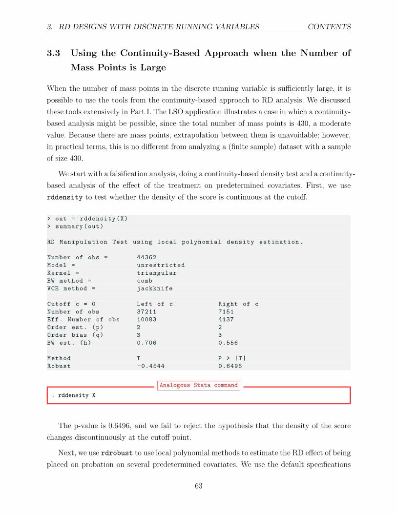
3. RD DESIGNS WITH DISCRETE RUNNING VARIABLES CONTENTS
3.3 Using the Continuity-Based Approach when the Number of
Mass Points is Large
When the number of mass points in the discrete running variable is sufficiently large, it is
possible to use the tools from the continuity-based approach to RD analysis. We discussed
these tools extensively in Part I. The LSO application illustrates a case in which a continuity-
based analysis might be possible, since the total number of mass points is 430, a moderate
value. Because there are mass points, extrapolation between them is unavoidable; however,
in practical terms, this is no different from analyzing a (finite sample) dataset with a sample
of size 430.
We start with a falsification analysis, doing a continuity-based density test and a continuity-
based analysis of the effect of the treatment on predetermined covariates. First, we use
rddensity to test whether the density of the score is continuous at the cutoff.
> out = rddensity(X)
> summary(out)
RD Manipulation Test using local polynomial density estimation.
Number of obs = 44362
Model = unrestricted
Kernel = triangular
BW method = comb
VCE method = jackknife
Cutoff c = 0 Left of c Right of c
Number of obs 37211 7151
Eff. Number of obs 10083 4137
Order est. (p) 2 2
Order bias (q) 3 3
BW est. (h) 0.706 0.556
Method T P > |T|
Robust -0.4544 0.6496
Analogous Stata command
. rddensity X
The p-value is 0.6496, and we fail to reject the hypothesis that the density of the score
changes discontinuously at the cutoff point.
Next, we use rdrobust to use local polynomial methods to estimate the RD effect of being
placed on probation on several predetermined covariates. We use the default specifications
63

3. RD DESIGNS WITH DISCRETE RUNNING VARIABLES CONTENTS
in rdrobust, that is, a MSE-optimal bandwdith that is equal on each side of the cutoff, a
triangular kernel, a polynoimial of order one, and a regularization term.
For example, we can estimate the RD effect of probation on hsgrade pct, the measure
of high school performance.
> out = rdrobust(data$hsgrade_pct , X)
> summary(out)
Call: rdrobust
Number of Obs. 44362
BW type mserd
Kernel Triangular
VCE method NN
Number of Obs. 37211 7151
Eff. Number of Obs. 6115 3665
Order est. (p) 1 1
Order bias (p) 2 2
BW est. (h) 0.465 0.465
BW bias (b) 0.759 0.759
rho (h/b) 0.612 0.612
=============================================================================
Method Coef. Std. Err. z P>|z| [ 95% C.I. ]
=============================================================================
Conventional 1.328 1.010 1.315 0.189 [ -0.652 , 3.309]
Robust - - 1.298 0.194 [ -0.788 , 3.878]
=============================================================================
Analogous Stata command
. rdrobust hsgrade_pct X
And we can also explore the RD effect graphically using rdplot.
> rdplot(data$hsgrade_pct , X, x.label = "Score", y.label = "",
+ title = "")
Analogous Stata command
. rdplot hsgrade_pct X
64

3. RD DESIGNS WITH DISCRETE RUNNING VARIABLES CONTENTS
Figure 3.2: RD plot for hsgrade pct—LSO data
●●●
●
●
●
●
●●
●
●●
●●
●
●
●
●
●
●
●
●
●
●
●
●
●
●
●
●
●
●
●
●
●
●
●
●
●●●
●
●
●
●
●
●
●
●
●
●
●●
●
●
●●
●
●
●●
●
●
●
●●
●
●●
●
●
●
●
●
●
●●
●●
●●
●
●
●
●●●●
●
●
●
●
●
●
●●
●
●
●●
●
●
●
●
●
●●
●
●●
●
●
●
●
●
●●
●
●
●
●
●●●
●●
●
●
●
●
●
●
●
●●
●
●
●
●
●
●
●
●
●
●
●
●●
●
●
●
●●
●
●
●
●
●
●●●
●
●●●
●●●
●
●
●
●
●
●
●●
●●
●
●
●
●●
●●●
●
●
●
●
●
●
●
●
●
●
●
●
●
●
●
●
●●●●●
●
●
●
●
●
●
●
●●
●
●
●
●
●
●●●●
●
●
●
●●●
●
●
●
●
●
●
●
●
●
●
●●●
●
●●
●●
●
●
●
●
●
●●●
●
●
●●
●
●●
●
●●●●
●
●
●
●●
●●
●
●
●
●
●
●
●●
●
●
●
●
●
●
●
●
●
●●
●
●
●
●
●
●
●
●
●●
●●●
●●
●
●●
●●●
●●
●●
●●
●
●●
●
●●
●●
●●
●
●
●
●
●
●●●●
●
●
●
●
●
●
●
●
●
●
●
●●
●
●
●
●●
●
●
●
●
●
●
●
●
●
●
●
●
●
●
●
●
●
●
●
●
●●
●
●
●
●
●
●
●
●
●
●
●
●
●
●
●
●
●
●
●
●●
●
●
●
●
●
●
●
●●●●
●
●
●
●●
●
●
●
●
●
●
●
●
●
●●
●
−2 −1 0 1
2040
6080
100
Score
Both the formal analysis and the graphical analysis indicate that, according to this
continuity-based local polynomial analysis, the students right above and below the cutoff
are similar in terms of their high school performance.
We repeat this analysis for the nine predetermined covariates mentioned above. Table 3.3
presents a summary of the results, and Figure 3.3 shows the associated RD plots for six of
the nine covariates.
Table 3.3: RD Effects on Predetermined Covariates—LSO data, Continuity-Based Approach
VariableMSE-Optimal RD Robust Inference Number of
Bandwidth Estimator p-value Conf. Int. Observations
High school grade percentile 0.465 1.328 0.194 [-0.788, 3.878] 9780Credits attempted in first year 0.301 0.081 0.005 [0.027, 0.157] 6443Age at entry 0.463 0.017 0.637 [-0.060, 0.099] 9780Male 0.482 -0.012 0.506 [-0.067, 0.033] 10121Born in North America 0.505 0.014 0.374 [-0.018, 0.049] 10757English is first language 0.531 -0.035 0.085 [-0.083, 0.005] 11239At Campus 1 0.289 -0.020 0.356 [-0.093, 0.034] 5985At Campus 2 0.476 -0.018 0.333 [-0.063, 0.021] 9910At Campus 3 0.271 0.036 0.139 [-0.015, 0.109] 5786
65

3. RD DESIGNS WITH DISCRETE RUNNING VARIABLES CONTENTS
Figure 3.3: RD Plots for Predetermined Covariates—LSO Application●●●
●
●
●
●
●●
●
●●
●●
●
●
●
●
●
●
●
●
●
●
●
●
●
●
●
●
●
●
●
●
●
●
●
●
●●●
●
●
●
●
●
●
●
●
●
●
●●
●
●
●●
●
●
●●
●
●
●
●●
●
●●
●
●
●
●
●
●
●●
●●
●●
●
●
●
●●●●
●
●
●
●
●
●
●●
●
●
●●
●
●
●
●
●
●●
●
●●
●
●
●
●
●
●●
●
●
●
●
●●●
●●
●
●
●
●
●
●
●
●●
●
●
●
●
●
●
●
●
●
●
●
●●
●
●
●
●●
●
●
●
●
●
●●●
●
●●●
●●●
●
●
●
●
●
●
●●
●●
●
●
●
●●
●●●
●
●
●
●
●
●
●
●
●
●
●
●
●
●
●
●
●●●●●
●
●
●
●
●
●
●
●●
●
●
●
●
●
●●●●
●
●
●
●●●
●
●
●
●
●
●
●
●
●
●
●●●
●
●●
●●
●
●
●
●
●
●●●
●
●
●●
●
●●
●
●●●●
●
●
●
●●
●●
●
●
●
●
●
●
●●
●
●
●
●
●
●
●
●
●
●●
●
●
●
●
●
●
●
●
●●
●●●
●●
●
●●
●●●
●●
●●
●●
●
●●
●
●●
●●
●●
●
●
●
●
●
●●●●
●
●
●
●
●
●
●
●
●
●
●
●●
●
●
●
●●
●
●
●
●
●
●
●
●
●
●
●
●
●
●
●
●
●
●
●
●
●●
●
●
●
●
●
●
●
●
●
●
●
●
●
●
●
●
●
●
●
●●
●
●
●
●
●
●
●
●●●●
●
●
●
●●
●
●
●
●
●
●
●
●
●
●●
●
−2 −1 0 1
2040
6080
100
Score
(a) High School Grade Percentile
●
●
●
●
●
●
●
●
●
●
●
●●
●
●
●
●
●
●
●
●
●
●
●
●
●
●
●
●
●
●
●●
●
●
●
●
●
●
●
●
●
●
●
●
●
●●
●
●
●
●
●●●●
●●
●
●
●
●
●
●●
●
●
●
●
●
●
●
●
●
●
●
●
●
●
●
●
●
●
●
●
●
●
●
●
●
●
●
●●
●
●●●
●
●
●
●
●
●
●
●
●
●
●
●
●
●
●
●
●
●
●●
●
●
●
●
●
●
●●
●
●
●
●
●
●
●
●●
●●●
●
●
●
●
●
●
●
●
●
●
●
●
●
●
●
●●●
●●
●
●
●
●
●
●
●
●
●
●
●
●
●
●
●
●
●
●
●
●
●
●
●
●
●
●
●
●
●●
●
●
●
●
●
●●
●
●
●
●
●
●
●
●
●
●
●
●
●
●
●
●
●
●
●
●●
●●
●
●
●
●
●
●
●
●
●
●
●
●
●
●
●
●
●
●●
●
●
●
●
●
●●
●●
●
●
●
●
●
●
●
●●
●
●
●
●
●
●
●
●●
●●●
●
●
●
●
●
●
●
●
●
●
●
●
●
●
●
●●
●
●●
●
●
●
●
●
●
●
●
●
●
●
●
●
●
●
●
●
●
●
●
●
●
●
●
●
●
●●
●
●●
●
●
●
●
●
●●
●
●
●
●
●
●
●
●
●
●
●
●●
●
●
●
●
●
●
●●
●
●
●
●
●
●
●●
●
●
●
●●
●
●
●
●
●
●●
●
●
●
●
●●●
●
●
●
●
●
●●
●
●●
●
●
●
●
●
●
●
●
●
●●
●
●
●
●
●
●
●
●
●
●
●
●
●
●
●
●
●
●
●
●
●
●
●
●
●
●
●
●
●
●
●
●●
●
●
●
−2 −1 0 1
3.0
3.5
4.0
4.5
5.0
5.5
Score
(b) Total Credits in First Year
●
●
●
●
●
●
●
●
●
●
●
●
●●
●
●
●●●
●
●
●
●
●
●
●
●●
●
●
●
●
●
●
●
●●
●
●
●
●
●
●
●●
●
●
●
●
●
●
●
●●
●
●
●
●●
●
●
●●●
●●
●
●
●
●●●●
●
●●
●
●
●
●
●●
●
●
●●
●●
●
●●●●
●
●
●
●●
●●●
●
●
●
●
●
●●●●●
●
●
●●●●
●●
●
●●●●
●●
●●
●
●●●
●●
●●
●
●
●
●●
●
●
●●●
●
●●●
●
●
●
●
●
●
●
●●●●●●●
●●●●●●●
●●●●
●●●
●
●●●
●●●
●
●
●
●
●●●
●
●
●●●●●
●
●●
●
●●
●
●
●●●
●
●
●●
●●●
●●●
●●
●
●●
●
●
●
●
●●
●
●
●
●●
●●
●
●
●
●●●●
●
●
●
●●
●●
●●●
●
●
●●
●
●
●
●
●
●●
●●
●
●
●
●
●●
●●
●
●
●
●
●
●
●
●
●●
●
●●
●
●
●
●
●
●●●●
●●●
●●
●●
●
●
●
●●●
●
●
●
●
●
●
●
●●
●
●
●
●●
●
●
●
●●
●
●●
●
●
●
●
●
●
●
●
●
●
●●
●
●●●
●
●
●●
●
●
●
●
●●
●
●
●
●
●
●
●
●
●
●
●
●
●
●
●●
●
●
●
●
●●
●
●
●
●
●
●
●
●
●
●
●
●
●
●
●●
●
●
●●
●
●
●
●
●
●
●
●
●
●
●
●
●
●
●
●
●●●
●
●
●
●
●●
●
●
●
●
−2 −1 0 1
18.0
18.5
19.0
19.5
20.0
20.5
Score
(c) Age at Entry
●
●
●
●
●
●
●
●
●
●
●
●
●●
●
●
●
●
●
●
●
●
●
●
●
●
●
●
●
●
●●
●
●
●
●
●
●
●●
●
●
●
●
●
●
●
●
●
●●●
●
●
●
●
●
●●
●
●
●
●●
●
●
●
●●
●
●
●
●
●
●
●
●
●●●
●
●
●
●
●
●
●
●
●
●
●
●
●
●
●
●
●
●●●
●
●
●
●
●
●
●
●
●
●
●
●
●
●
●
●
●
●
●
●
●
●
●
●
●
●
●
●●
●
●
●
●
●
●
●
●
●
●
●
●●
●
●
●
●
●
●
●●●
●
●
●
●
●
●
●
●●
●
●
●
●
●
●
●
●●
●
●
●
●●
●
●
●
●
●
●
●
●
●
●
●
●
●
●
●●●
●
●
●
●
●
●
●●
●
●
●
●
●
●
●
●●
●
●
●
●
●
●
●●
●
●
●
●
●
●
●
●
●●
●
●●
●
●
●
●●
●
●
●●
●
●●
●
●
●
●
●●
●
●●
●●
●
●
●
●
●
●
●
●
●
●
●
●
●
●
●
●
●
●
●
●●
●
●
●
●
●
●
●
●
●
●●
●
●
●
●
●
●
●
●
●
●
●
●
●
●●
●
●●
●●
●
●
●●
●●
●
●
●●
●
●
●
●
●
●
●
●
●●●
●
●
●
●
●
●
●
●
●
●
●
●
●
●
●
●●
●
●
●
●
●
●
●
●
●●
●
●●●
●
●
●
●
●
●
●
●
●
●
●●
●
●
●
●
●●
●
●
●
●
●
●
●
●
●
●●
●●
●
●
●
●
●
●●
●
●
●
●
●
●
●●
●
●●
●
●
●
●
●
●
●●
●
●
●
●
●
●
●
●
●
●
●
●
●
●
●●
●
−2 −1 0 1
0.0
0.2
0.4
0.6
0.8
1.0
Score
(d) English First Language Indicator
●
●
●
●
●
●
●
●
●
●
●
●
●
●
●
●
●
●
●
●
●
●
●
●
●●
●
●
●
●●
●
●
●●
●
●
●
●
●
●
●
●
●
●
●
●
●●
●
●
●●
●
●
●
●●
●●
●
●●●
●
●●
●
●●
●
●
●
●
●●
●
●
●
●
●
●
●
●
●
●
●
●
●
●
●●
●
●
●
●
●
●
●
●
●●●●
●
●
●
●
●
●
●
●
●
●
●
●
●
●
●●●●●
●
●
●
●
●
●
●●
●
●
●
●
●
●
●
●
●
●
●
●
●
●
●●
●●
●
●
●
●
●
●
●●●
●
●
●
●
●
●
●
●●●
●
●●
●●
●
●
●
●●
●
●
●
●
●
●
●●
●
●
●
●●
●
●
●
●
●
●●●
●●
●
●
●
●
●
●
●
●●●
●
●
●
●
●
●
●
●
●
●
●
●
●●
●
●
●●
●
●
●
●
●●
●
●
●
●●
●
●
●
●
●
●●
●
●
●●
●
●
●●
●
●
●
●
●
●
●●
●
●●●●
●
●
●
●
●
●
●
●
●
●
●
●
●
●
●
●
●
●
●
●
●
●
●
●●
●●
●
●
●
●
●
●
●
●
●
●
●
●
●
●
●
●
●
●●
●
●
●
●
●
●
●
●
●
●
●
●
●
●
●
●
●
●
●
●
●
●
●
●
●
●
●
●●
●
●
●●
●
●
●
●
●
●
●●
●
●
●
●
●●
●●
●
●
●
●
●
●●
●
●
●
●
●
●
●
●
●
●
●●
●
●
●
●
●
●
●
●
●
●
●
●
●
●
●
●
●
●●
●●
●
●
●
●
●
●
●
●
●●
●
●
●
●
●
●
●
●
●
●
●
●
●
●
●●
●
−2 −1 0 1
0.0
0.2
0.4
0.6
0.8
1.0
Score
(e) Male Indicator
●
●
●
●
●
●
●
●
●
●
●
●
●●●
●
●
●
●
●
●
●
●
●
●●
●
●
●
●
●●
●
●
●
●
●●
●●
●
●
●
●
●
●
●
●●
●
●
●●●
●
●●●
●
●
●
●
●●
●
●●
●
●
●
●
●
●
●
●
●●
●●●
●
●
●
●
●●●
●
●
●
●●
●
●
●
●
●
●●
●●
●
●
●
●
●
●
●
●●
●
●
●●●
●
●
●
●
●
●
●
●
●
●
●
●
●
●
●
●●●
●
●
●
●
●
●
●
●●
●
●
●
●
●
●●●
●
●
●
●
●
●●●●
●●●●
●
●
●
●
●●
●
●
●
●
●
●
●
●
●
●●
●●
●
●●
●
●
●
●
●
●●
●●
●
●
●
●●
●
●
●
●
●
●
●●●●●
●
●
●
●●●
●
●
●
●●●●●
●
●
●●
●
●●
●
●
●
●
●
●
●●
●
●●
●
●
●
●●
●●
●
●
●●
●
●
●
●
●●
●
●
●●●
●
●
●
●
●
●
●
●
●
●
●
●
●●
●●
●
●
●
●
●
●
●
●●
●●
●
●
●
●
●
●●
●
●
●
●●
●
●
●
●
●
●
●
●
●
●●
●●
●
●
●
●
●
●
●
●
●●
●
●
●
●
●
●
●
●
●
●
●
●
●●
●
●
●
●
●
●
●
●
●
●
●
●
●
●
●
●
●
●
●
●
●
●●●
●
●
●
●
●
●
●
●●
●
●
●
●
●
●
●
●
●
●
●●
●
●
●
●●
●
●●
●
●
●
●
●
●
●
●
●●
●
●
●
●
●
●
●
●
●
●
●
●
●
●
●
●
●
●
●
●
●●
●
●
●
●
●
−2 −1 0 1
0.0
0.2
0.4
0.6
0.8
1.0
Score
(f) Born in North America Indicator
66

3. RD DESIGNS WITH DISCRETE RUNNING VARIABLES CONTENTS
Overall, the results indicate that the probation treatment has no effect on the prede-
termined covariates, with two exceptions. First, the the effect on totcredits year1 has
associated p-value 0.004, rejecting the hypothesis of no effect at standard levels. However,
the point estimate is small: treated students take an additional 0.081 credits in the first year,
but the average value of totcredits year1 in the overall sample is 4.43, with a standard
deviation of roughly 0.5. Second, students who are placed on probation are 3.5 percentage
points less likely to speak English as a first language, an effect that is significant at 10%.
This difference is potentially more worrisome, and is also somewhat noticeable in the RD
plot in Figure 3.3(d).
Next, we analyze the effect of being placed on probation on the outcome of interest,
nextGPA, the GPA in the following academic term. We first use rdplot to visualize the
effect.
> out = rdplot(nextGPA_nonorm , X, binselect = "esmv")
> summary(out)
Call: rdplot
Number of Obs. 40582
Kernel Uniform
Number of Obs. 34854 5728
Eff. Number of Obs. 34854 5728
Order poly. fit (p) 4 4
BW poly. fit (h) 2.800 1.600
Number of bins scale 1 1
Bins Selected 690 362
Average Bin Length 0.004 0.004
Median Bin Length 0.004 0.004
IMSE -optimal bins 44 13
Mimicking Variance bins 690 362
Relative to IMSE -optimal:
Implied scale 15.682 27.846
WIMSE variance weight 0.000 0.000
WIMSE bias weight 1.000 1.000
Analogous Stata command
. rdplot nextGPA_nonorm X, binselect(esmv) ///
> graph_options(graphregion(color(white)) ///
> xtitle(Score) ytitle(Outcome))
67

3. RD DESIGNS WITH DISCRETE RUNNING VARIABLES CONTENTS
●
●
●●●●
●●●
●
●●●
●
●
●
●●●
●
●
●
●
●
●
●●
●
●
●
●●●
●
●●●●
●
●●●●●
●
●●●●●
●
●
●
●
●●●●
●●
●●●●●●●●●
●
●●●●
●
●
●
●●●●●●●●
●
●●●●●
●
●
●
●
●
●
●●●
●●●●●●
●●●
●●●●
●●●●
●●
●
●●
●●
●●
●●●●●●
●
●●●
●●
●
●●●●
●●
●●
●
●
●
●
●●
●
●●●●●
●●
●●●
●●●●●●●●
●●●●●
●●●
●●
●●●●
●
●●●●
●
●
●●●●●●●●
●
●
●●
●●
●●
●
●
●
●
●●
●●●●
●
●
●●
●●●●●●●
●●●●●●
●
●●●
●●
●●
●
●
●●
●●
●
●
●
●●●
●
●
●
●●●●●●●
●
●
●
●●
●●●
●●
●
●●
●
●●●●●●●
●
●●
●●
●
●●
●
●●●
●
●
●
●
●●●●
●●●
●
●
●●●
●●
●
●
●
●
●
●●●
●
●
●●
●●●●●●
●
●
●
●
●
●
●
●●
●
●
●
●●
●
●
●
●
●
●●
●
●
●●
●
●
●●
●
●
●
●
●
●
●
●
●
●
●
●
●
●
●
●
●
●
●
●
●
●
●
●
●
●
●
●
●
●
●
●
●
●
●
●
●
●
●
●
●
●
●
●
●●
●
●
●
●
●
●
●
●
●
●
●
●
●
●
●
●
●
●
●
−2 −1 0 1
01
23
4
Score
Out
com
e
Figure 3.4: RD Plot for nextGPA—LSO Data
Overall, the plot shows a very clear negative relationship between the running variable
and the outcome: students who have a low GPA in the current (and thus have a higher value
of the running variable) tend to also have a low GPA in the following term. The plot also
shows that students with scores just above the cutoff (who are just placed on probation)
tend to have a higher GPA in the following term relative to students who are just below the
cutoff and just avoided probation. These results are confirmed when we use a local linear
polynomial and robust inference to provide a formal statistical analysis of the RD effect.
> out = rdrobust(nextGPA_nonorm , X, kernel = "triangular", p = 1,
+ bwselect = "mserd")
> summary(out)
Call: rdrobust
Number of Obs. 40582
BW type mserd
Kernel Triangular
VCE method NN
Number of Obs. 34854 5728
Eff. Number of Obs. 5249 3038
Order est. (p) 1 1
Order bias (p) 2 2
BW est. (h) 0.437 0.437
BW bias (b) 0.717 0.717
rho (h/b) 0.610 0.610
=============================================================================
68

3. RD DESIGNS WITH DISCRETE RUNNING VARIABLES CONTENTS
Method Coef. Std. Err. z P>|z| [ 95% C.I. ]
=============================================================================
Conventional 0.222 0.040 5.615 0.000 [0.145 , 0.300]
Robust - - 4.572 0.000 [0.122 , 0.304]
=============================================================================
Analogous Stata command
. rdrobust nextGPA_nonorm X, kernel(triangular) p(1) bwselect(mserd)
As shown, students who are just placed on probation improve their GPA in the following
term by 0.2221 additional points, relative to students who just missed probation. The robust
p-value is less than 0.00005, and the robust 95% confidence interval ranges from 0.1217 to
0.3044. Thus, the evidence indicates that, conditional on not leaving the university, being
placed on academic probation translates into an increase in future GPA. The point estimate
of 0.2221—oobtained with rdrobust within a MSE-optimal bandwidth of 0.4375—is very
similar to the effect of 0.23 grade points found by LSO within an ad-hoc bandwidth of 0.6.
To better understand this effect, we may be interested in knowing the point estimate
for the controls and treated students separetely. To see this information, we explore the
information returned by rdrobust.
> rdout = rdrobust(nextGPA_nonorm , X, kernel = "triangular", p = 1,
+ bwselect = "mserd")
> print(names(rdout))
[1] "Estimate" "bws" "coef" "bws" "se" "z" "pv
" "ci" "h_l" "h_r" "b_l" "b_r" "N_h_l"
"N_h_r" "beta_p_l" "beta_p_r" "V_cl" "V_rb" "N" "
Nh" "Nb" "c" "p" "q" "bias" "beta_
p"
[27] "kernel" "vce" "bwselect" "level" "all" "call"
> print(rdout$beta_p_r)
[,1]
[1,] 2.0671526
[2,] -0.6713546
> print(rdout$beta_p_l)
[,1]
[1,] 1.8450372
[2,] -0.6804159
Analogous Stata command
. rdrobust nextGPA_nonorm X
. ereturn list
69

3. RD DESIGNS WITH DISCRETE RUNNING VARIABLES CONTENTS
This output shows the estimated intercept and slope from the two local regressions esti-
mated separately to the rigth (beta p r) and left (beta p l) of the cutoff. At the cutoff, the
average GPA in the following term for control students who just avoid probation is 1.8450372
, while the average future GPA for treated students who are just placed on probation is
2.0671526. The increase is the estimated RD effect reported above, 2.0671526− 1.8450372 =
0.2221154. This represents approximately a 12% GPA increase relative to the control group,
a considerable effect.
An alternative to the simplest use of rdrobust illustrated above is to cluster the standard
errors by every value of the score—this is the approach recommended by Lee and Card (2008),
as we discuss in the Further Readings section below. We implement this using the cluster
option in rdrobust.
> clustervar = X
> out = rdrobust(nextGPA_nonorm , X, kernel = "triangular", p = 1,
+ bwselect = "mserd", vce = "hc0", cluster = clustervar)
> summary(out)
Call: rdrobust
Number of Obs. 40582
BW type mserd
Kernel Triangular
VCE method HC0
Number of Obs. 34854 5728
Eff. Number of Obs. 4357 2709
Order est. (p) 1 1
Order bias (p) 2 2
BW est. (h) 0.377 0.377
BW bias (b) 0.627 0.627
rho (h/b) 0.602 0.602
=============================================================================
Method Coef. Std. Err. z P>|z| [ 95% C.I. ]
=============================================================================
Conventional 0.215 0.033 6.463 0.000 [0.150 , 0.280]
Robust - - 5.396 0.000 [0.132 , 0.282]
=============================================================================
Analogous Stata command
. gen clustervar=X
. rdrobust nextGPA_nonorm X, kernel(triangular) p(1) bwselect(mserd) vce(cluster clustervar)
The conclusions remain essentially unaltered, as the 95% robust confidence interval
70

3. RD DESIGNS WITH DISCRETE RUNNING VARIABLES CONTENTS
changes only slightly from [0.1217 , 0.3044] to [0.1316 , 0.2818]. Note that the point estimate
moves slightly from 0.2221 to 0.2149 because the MSE-optimal bandwidth with clustering
shrinks to 0.3774 from 0.4375, and the bias bandwidth also decreases.
3.4 Interpreting Continuity-Based RD Analysis with Mass Points
Provided that the number of mass points in the score is reasonably large, it is possible
to analyze an RD design with a discrete score using the tools from the continuity-based
approach. However, it is important to understand how to correctly interpret the results from
such analysis. We now analyze the LSO application further, with the goal of clarifying these
issues.
When there are mass points in the running variable, local polynomial methods for RD
analysis behave essentially as if we had as many observations as mass points, and therefore the
method implies extrapolation from the closest mass point on either side to the cutoff. In other
words, when applied to a RD design with a discrete score, the effective number of observations
used by continuity-based methods is the number of mass points or distinct values, not the
total number of observations. Thus, in practical terms, fitting a local polynomial to the raw
data with mass points is roughly equivalent to fitting a local polynomial to a “collapsed”
version of the data, where we aggregate the original observations by the discrete score values,
calculating the average outcome for all observations that share the same score value. Thus,
the total number of observations in the collapsed dataset is equal to the number of mass
points in the running variable.
To illustrate this procedure with the LSO data, we calculate the average outcome for
each of the 430 mass points in the score value. The resulting dataset has 430 observations,
where each observation consists of a score-outcome pair: every score value is paired with the
average outcome across all students in the original dataset whose score is equal to that value.
When then use rdrobust to estimate the RD effect with a local polynomial.
> data2 = data.frame(nextGPA_nonorm , X)
> dim(data2)
[1] 44362 2
> collapsed = aggregate(nextGPA_nonorm ~ X, data = data2 , mean)
> dim(collapsed)
[1] 429 2
> out = rdrobust(collapsed$nextGPA_nonorm , collapsed$X)
> summary(out)
Call: rdrobust
Number of Obs. 429
71

3. RD DESIGNS WITH DISCRETE RUNNING VARIABLES CONTENTS
BW type mserd
Kernel Triangular
VCE method NN
Number of Obs. 274 155
Eff. Number of Obs. 51 50
Order est. (p) 1 1
Order bias (p) 2 2
BW est. (h) 0.506 0.506
BW bias (b) 0.805 0.805
rho (h/b) 0.628 0.628
=============================================================================
Method Coef. Std. Err. z P>|z| [ 95% C.I. ]
=============================================================================
Conventional 0.246 0.032 7.640 0.000 [0.183 , 0.309]
Robust - - 6.279 0.000 [0.166 , 0.316]
=============================================================================
Analogous Stata command
. collapse (mean) nextGPA_nonorm, by(X)
. rdrobust nextGPA_nonorm X
The estimated effect is 0.2456, with robust p-value less than 0.00005. This is similar to the
0.2221 point estimate obtained with the raw dataset. The similarity between the two point
estimates is remarkable,considering that the former was calculated using 430 observations,
while the latter was calculated using 40, 582 observations, more than a ninety-fold increase.
Indeed, the inference conclusions from both analysis are extremely consistent, as the robust
95% confidence interval using the raw data is [0.1217 , 0.3044], while the robust confidence
interval for the collapsed data is [0.1659, 0.3165], both indicating that the plausible values
of the effect are in roughly the same positive range.
This analysis shows that the seemingly large number of observations in the raw dataset
is effectively much smaller, and that the behavior of the continuity-based results is governed
by the average behavior of the data at every mass point. Thus, a natural point of departure
for researchers who wish to study a discrete RD design with many mass points is to collapse
the data and estimate the effects on the aggregate results. As a second step, these aggregate
results can be compared to the results using the raw data—in most cases, both sets of results
should lead to the same conclusions.
While the mechanics of local polynomial fitting using a discrete running variable are clear
now, the actual relevance and interpretation of the treatment effect may change. As we will
72

3. RD DESIGNS WITH DISCRETE RUNNING VARIABLES CONTENTS
discuss below, researchers may want to change the parameter of interest altogether when the
score is discrete. Alternatively, (parametric) extrapolation is unavoidable to point identifica-
tion. To be more precise, because the score is discrete, it is not possible to nonparametrically
point identify the vertical distance between τSRD = E[Yi(1)|Xi = x] − E[Yi(0)|Xi = x], even
asymptotically, because conceptually the lack of denseness in Xi makes it impossible to ap-
peal to large sample approximations. Put differently, if researchers insist on retaining the
same parameter of interest as in the canonical RD design, then extrapolation from the closest
mass point to the cutoff will be needed, no matter how large the sample size is.
Of course, there is no reason why the same RD treatment effect would be of interest when
the running variable is discrete or, if it is, then any extrapolation method would be equally
valid. Thus, continuity-based methods, that is, simple local linear extrapolation towards
the cutoff point is natural and intuitive. When only a few mass points are present, then
bandwidth selection makes little sense, and the research may just conduct linear (parametric)
extrapolation globally, as this is essentially the only possibility, if the goal is to retain the
same canonical treatment effect parameter.
3.5 Local Randomization RD Analysis with Discrete Score
A natural alternative to analyze an RD design with a discrete running variable is to use the
local randomization approach, which effectively changes the parameter of interest from the
RD treatment effect a the cutoff to the RD treatment effect in the neighborhood around
the cutoff where local randomization is assumed to hold. A key advantage of this alternative
conceptual framework is that, unlike the continuity-based approach illustrated above, it can
be used even when there are very few mass points in the running variable: indeed, it can be
used with as few as two mass points.
To compare the change in RD parameter of interest, consider the extreme case where the
score takes five values −2,−1, 0, 1, 1 and the RD cutoff is x = 0. Then, the continuity-based
parameter of interest is τSRD = E[Yi(1)|Xi = 0]− E[Yi(0)|Xi = 0], which is not nonparamet-
rically identifiable, because the score of control observations can never get close enough to
0. However, if the true window is, say, W0 = [−1, 0], the local randomization parameter will
be τLR = E[Yi(1)|Xi = 0] − E[Yi(0)|Xi = −1], which is nonparametrically identifiable under
the conditions discussed in Section 2. Going from τLR to τSRD requires extrapolating from
E[Yi(0)|Xi = −1] to E[Yi(0)|Xi = 0], which is impossible without additional assumptions
even in large samples because of the intrinsic discreteness of the running variable. In some
specific applications, additional features may allow researchers to extrapolate (e.g., round-
73

3. RD DESIGNS WITH DISCRETE RUNNING VARIABLES CONTENTS
ing), but in general extrapolation will require additional restrictions on the data generating
process. Furthermore, from a conceptual point of view, it can be argued that the parameter
τLR is more interesting and policy relevant than the parameter τSRD when the running variable
is discrete.
When the score is discrete using the local randomization approach for inference does not
require choosing a window in most applications. In other words, with a discrete running
variable the researcher knows the exact location of the minimum window around the cutoff:
this window is the interval of the running variable that contains the two mass points, one
on each side of the cutoff, that are immediately consecutive to the cutoff value. Crucially,
if local randomization holds, then it must hold for the smallest window in the absence of
design failures such as manipulation of the running variable. To illustrate, as shown in Table
3.2, in the LSO application the original score has a mass point at zero where all observations
are control (because they reach the minimum GPA required to avoid probation), and the
mass point immediately below it occurs at -0.01, where all students are placed on probation
because they fall short of the threshold to avoid probation. Thus, the smallest window around
the cutoff in the scale of the original score is W0 = [0.00,−0.01]. Analogously, in the scale
of the transformed score, the minimum window is W0 = [−0.000005, 0.01].
Regardless of the scale used, the important point is that the minimum window around
the cutoff in a local randomization analysis of an RD with a discrete score is precisely the
interval between the two consecutive mass points where the treatment status changes from
zero to one. Note that the particular values taken by the score are irrelevant, as the analysis
will proceed to assume that the treated and control groups were assigned to treatment as-if
randomly, and will typically make the exclusion restriction assumption that the particular
value of the score has no direct impact on the outcome of interest. Moreover, the location
of the cutoff is no longer meaningful, as any value of the cutoff between the minimum value
of the score on the treated side and the maximum value of the score in the control side will
produce identical treatment and control groups.
Once the researcher finds the treated and control observations located at the two mass
points around the cutoff, the local randomization analysis can proceed as explained in Section
2. We first conduct a falsification analysis, to determine whether the assumption of local
randomization in the window [−0.00005, 0.1] seems consistent with the empirical evidence.
We conduct a density test using the rdwinselect function using the option nwindows=1 to
see only results for this window, to test whether the density of observations in this window is
consistent with the density that would have been observed in a series of unbiased coin flips.
74

3. RD DESIGNS WITH DISCRETE RUNNING VARIABLES CONTENTS
> out = rdwinselect(X, wmin = 0.01, nwindows = 1, cutoff = 5e-06)
Window selection for RD under local randomization
Number of obs = 44362
Order of poly = 0
Kernel type = uniform
Reps = 1000
Testing method = rdrandinf
Balance test = diffmeans
Cutoff c = 0 Left of c Right of c
Number of obs 37211 7151
1st percentile 298 0
5th percentile 1817 269
10th percentile 3829 663
20th percentile 7588 1344
Window length / 2 p-value Var. name Bin.test Obs <c
Obs >=c
0.01 NA NA 0 228
77
Analogous Stata command
. rdwinselect X, wmin(0.01) nwindows(1) cutoff(0.000005)
As shown in the rdwinselect output and also showed previously in Table 3.2, there are
228 control observations immediately below the cutoff, and 77 above the cutoff. In other
words, there are 228 students who get exactly the minimum GPA needed to avoid probation,
and 77 students who get the maximum possible GPA that still places them on probation. The
number of control observations is roughly three times higher than the number of treated ob-
servations, a ratio that is inconsistent with the assumption that the probability of treatment
assignment in this window was 1/2—the p-value of the Binomial test reported in column
Bin. test is indistinguishable from zero.
We can also obtain this result by using the Binomial test commands directly.
> binom.test(77, 305, 1/2)
Exact binomial test
data: 77 and 305
number of successes = 77, number of trials = 305, p-value < 2.2e-16
alternative hypothesis: true probability of success is not equal to 0.5
95 percent confidence interval:
75

3. RD DESIGNS WITH DISCRETE RUNNING VARIABLES CONTENTS
0.2046807 0.3051175
sample estimates:
probability of success
0.252459
Analogous Stata command
. bitesti 305 77 1/2
Although these results alone do not imply that the local randomization RD assumptions
are violated, the fact that there are many more control than treated students is consistent
with what one would expect if students were actively avoiding an undesirable outcome. The
results raise some concern that students may have been aware of the probation cutoff, and
may have tried to appeal their final GPA in order to avoid being placed on probation.
Strictly speaking, an imbalanced number of observations would not pose any problems if
the types of students in the treated and control groups were on average similar. To establish
whether treated and control students at the cutoff are similar in terms of observable char-
acteristics, we use rdrandinf to estimate the RD effect of probation on the predetermined
covariates introduced above.
We report the full results for the covariate hsgrade pct.
> out = rdrandinf(data$hsgrade_pct , X, wl = -0.005, wr = 0.01,
+ seed = 50)
Selected window = [ -0.005;0.01]
Running randomization -based test ...
Randomization -based test complete.
Number of obs = 44362
Order of poly = 0
Kernel type = uniform
Reps = 1000
Window = set by user
H0: tau = 0
Randomization = fixed margins
Cutoff c = 0 Left of c Right of c
Number of obs 37211 7151
Eff. number of obs 228 77
Mean of outcome 29.118 32.675
S.d. of outcome 21.737 21.625
Window -0.005 0.01
76

3. RD DESIGNS WITH DISCRETE RUNNING VARIABLES CONTENTS
Finite sample Large sample
Statistic T P>|T| P>|T| Power vs d =
10.868
Diff. in means 3.557 0.219 0.213 0.968
Analogous Stata command
. rdrandinf hsgrade_pct X , seed(50) wl(-.005) wr(.01)
We repeated this analysis for all predetermined covariates, but do not present the in-
dividual runs to conserve space. A summary of the results is reported in Table 3.4. As
shown, treated and control students seem indistinguishable in terms of prior high school
performance, total number of credits, age, sex, and place of birth.
On the other hand, the Fisherain sharp null hypothesis is that the treatment has no effect
on the English-as-first-language indicator is rejected with p-value of 0.009. The average
differences in this variable are very large: 75% of control students speak English as first
language, but only 62.3% of treated students do. These difference is consistent with the local
polynomial results we reported for this variable in Table 3.3, although the difference is much
larger (an average difference of -3.5 percentage points in the continuity-based analysis, versus
an average difference of -15 percentage points in the local randomization analysis). A similar
phenomenon occurs for the Campus 2 and Campus 3 indicators, which appear imbalanced
in the local randomization analysis (with Fisherian p-values of 0.075 and 0.009) but appear
balanced with a continuity-based analysis.
These differences illustrate how a continuity-based analysis of a discrete RD design can
mask differences that occurs in mass points closest to the cutoff. In general, when analyzing
a RD design with a discrete running variable, it is advisable to perform falsification tests
with the two mass points closest to the cutoff in order to detect phenomena of sorting or
selection that may go unnoticed when a continuity-based approach is used.
77

3. RD DESIGNS WITH DISCRETE RUNNING VARIABLES CONTENTS
Table 3.4: RD Effects on Predetermined Covariates—LSO data, Local Randomization Ap-proach
VariableMean of Mean of Diff-in-Means Fisherian Number ofControls Treated Statistic p-value Observations
High school grade percentile 29.118 32.675 3.557 0.201 305Credits attempted in first year 4.228 4.318 0.090 0.157 305Age at entry 18.772 18.688 -0.084 0.421 305Male 0.377 0.442 0.064 0.336 305Born in North America 0.890 0.844 -0.046 0.322 305English is first language 0.772 0.623 -0.149 0.009 305At Campus 1 0.465 0.390 -0.075 0.259 305At Campus 2 0.241 0.143 -0.098 0.075 305At Campus 3 0.294 0.468 0.174 0.009 305
Finally, we also investigate the extent to which the particular window around the cutoff,
including only two mass points, is driving the empirical results by repeating the analysis
using different nested windows. These exercise is easily implemented using the command
rdwinselect:
> Z = cbind(data$hsgrade_pct , data$totcredits_year1 , data$age_at_entry ,
+ data$male , data$bpl_north_america , data$english , data$loc_campus1 ,
+ data$loc_campus2 , data$loc_campus3)
> colnames(Z) = c("hsgrade_pct", "totcredits_year1", "age_at_entry",
+ "male", "bpl_north_america", "english", "loc_campus1", "loc_campus2",
+ "loc_campus3")
> out = rdwinselect(X, Z, p = 1, seed = 50, wmin = 0.01, wstep = 0.01,
+ cutoff = 5e-06)
Window selection for RD under local randomization
Number of obs = 44362
Order of poly = 1
Kernel type = uniform
Reps = 1000
Testing method = rdrandinf
Balance test = diffmeans
Cutoff c = 0 Left of c Right of c
Number of obs 37211 7151
1st percentile 298 0
5th percentile 1817 269
10th percentile 3829 663
20th percentile 7588 1344
Window length / 2 p-value Var. name Bin.test Obs <c
Obs >=c
78

3. RD DESIGNS WITH DISCRETE RUNNING VARIABLES CONTENTS
0.01 0.008 loc_campus3 0 228
77
0.02 0 totcredits_year 0 298
214
0.03 0 hsgrade_pct 0 374
269
0.04 0 loc_campus1 0 494
375
0.05 0 totcredits_year 0 636
418
0.06 0 hsgrade_pct 0 714
497
0.07 0 hsgrade_pct 0 807
663
0.08 0 totcredits_year 0 877
727
0.09 0 totcredits_year 0 1049
815
0.1 0 totcredits_year 0.001 1131
973
Analogous Stata command
. rdwinselect X $covariates, cutoff(0.00005) wmin(0.01) wstep(0.01)
The empirical results continue to provide evidence of inbalance in at least one pre-
intervention covariate for each window consider, using randomization inference methods for
the difference in means test statistic.
To complete the empirical illustration, we investigate the local randomization RD treat-
ment effect on the main outcome of interest using rdrandinf.
> out = rdrandinf(nextGPA_nonorm , X, wl = -0.005, wr = 0.01, seed = 50)
Selected window = [ -0.005;0.01]
Running randomization -based test ...
Randomization -based test complete.
Number of obs = 40582
Order of poly = 0
Kernel type = uniform
Reps = 1000
Window = set by user
H0: tau = 0
Randomization = fixed margins
79

3. RD DESIGNS WITH DISCRETE RUNNING VARIABLES CONTENTS
Cutoff c = 0 Left of c Right of c
Number of obs 34854 5728
Eff. number of obs 208 67
Mean of outcome 1.83 2.063
S.d. of outcome 0.868 0.846
Window -0.005 0.01
Finite sample Large sample
Statistic T P>|T| P>|T| Power vs d =
0.434
Diff. in means 0.234 0.063 0.051 0.952
Analogous Stata command
. rdrandinf nextGPA_nonorm X, seed(50) wl(-0.005) wr(0.01)
Remarkably, the difference-in-means between the 208 control students and the 67 treated
students in the smallest window around the cutoff is 0.234 grade points, extremely similar
to the continuity-based local polynomial effects of 0.2221 and 0.2456 that we found using
the raw and aggregated data, respectively. (The discrepancy between the treated and control
sample sizes of 77 and 288 reported in Table 3.2 and the sample sizes of 67 and 208 reported
in the rdrandinf output occurs because there are missing values in the nextGPA outcome, as
students who leave the university do not have any future GPA.) Moreover, we can reject the
null hypothesis of no effect at 10% level using both the Fisherian and the Neyman inference
approaches. This shows that the results for next term GPA are remarkably robust: we found
very similar results using the 208 + 67 = 275 observations closest to the cutoff in a local
randomization analysis, the total 40, 582 observations using a continuity-based analysis, and
the 429 aggregated observations in a continuity-based analysis.
3.6 Further Readings
Lee and Card (2008) proposed alternative assumptions under which the local polynomial
methods in the continuity-based RD framework can be applied when the running variable
is discrete. Their method requires assuming a random specification error that is orthogonal
to the score, and modifying inferences by using standard errors that are clustered at each of
the different values taken by the score. Similarly, Dong (2015) discusses the issue rounding
in the running variable. Both approaches have in common that the score is assumed to be
inherently continuous, but somehow imperfectly measured—perhaps because of rounding
errors—in such a way that the dataset available to the researcher contains mass points.
80

3. RD DESIGNS WITH DISCRETE RUNNING VARIABLES CONTENTS
Cattaneo et al. (2015, Section 6.2) discuss explicitly the connections between discrete scores
and the local randomization approach; see also Cattaneo et al. (2017).
81

4. THE FUZZY RD DESIGN CONTENTS
4 The Fuzzy RD Design
We now discuss how to modify the analysis and interpretation of the RD design when some
units fail to comply with the treatment condition that is assigned to them. In all RD designs,
the assignment of treatment follows the rule Ti = 1(Xi ≥ x), which assigns all units whose
score is below the cutoff x to the control condition, and all units whose score is above x are to
the treatment condition. In the Sharp RD design we discussed in Part I, we assumed that (i)
all units assigned to the treatment condition do in fact take the treatment, and (ii) no units
assigned to the control condition take the treatment. In that case, the rule Ti = 1(Xi ≥ x)
indicates not only the treatment assigned to the units, but also the treatment received by
the units.
In practice, however, it is very common to encounter RD designs where some of the units
with Xi ≥ x fail to receive the treatment and/or some of the units with Xi < x receive
the treatment despite being assigned to the control condition. The phenomenon of units
receiving a treatment condition different from the condition that is originally assigned to
them is generally known as imperfect compliance or non-compliance. The RD design with
imperfect compliance is usually referred to as the Fuzzy RD design, to distinguish it from
the Sharp RD design where compliance with treatment is perfect. Imperfect compliance is
very common in controlled randomized experiments, and is no less common in RD designs.
The Fuzzy RD treatment assignment rule is still Ti = 1(Xi ≥ x). However, compliance
with treatment is imperfect. As a consequence, although the probability of receiving treat-
ment still jumps abruptly at the cutoff x, it no longer changes from 0 to 1 as in the Sharp
RD case. (Naturally, the probability of being assigned to treatment still jumps from 0 to 1
at x.) To describe this design in generality, we need to introduce additional notation. We
use the binary variable Di to denote whether the treatment was actually received by unit
i. Our notation now distinguishes between the treatment assigned, Ti, and the treatment
actually received, Di. Using this notation, we can say that the defining feature of the Fuzzy
RD design is that there are some units for which Ti 6= Di.
Because the treatment received is not always equal to the treatment assigned, now the
treatment received Di (also known as “treatment take-up”) has two potential values, Di(1)
and Di(0), corresponding, respectively, to the treatment taken when the unit is assigned
to treatment condition (i.e, when Xi ≥ x and Ti = 1) and the treatment taken when the
unit is assigned to the control condition (i.e, when Xi < x and Ti = 0). The observed
treatment taken is Di = Ti ·Di(1) + (1− Ti) ·Di(0) and, as occurred for the outcome Yi, the
fundamental problem of causal inference now means that we do not observe, for example,
82

4. THE FUZZY RD DESIGN CONTENTS
whether a unit that was assigned to the treatment condition and took the treatment would
have taken the treatment if it had been assigned to the control condition instead. The
potential outcomes under treatment and control are still denoted, respectively, Yi(1) and
Yi(0), although it is important to note that 1 and the 0 in the function Yi(·) now refer
to the treatment take-up status Di = 1 and Di = 0, respectively, not to the treatment
assignment status. Notice that our potential outcomes notation, (Yi(1), Yi(0)), also imposes
the restriction that the treatment assignment T has no direct effect on Y , since T is not
an argument in the potential outcome functions. The treatment assignment T affects the
outcome Y only because this assignment induces a change in the actual treatment taken D,
which in turns affects Y . This type of restriction is sometimes called exclusion restriction.
We illustrate the difference between the Sharp and Fuzzy RD designs is in Figure 4.1,
where we plot the conditional probability of receiving treatment given the score, P(Di =
1|Xi = x), for different values of the running variable Xi. As shown in Figure 4.1(a), in a
Sharp RD design the probability of receiving treatment changes exactly from zero to one at
the cutoff. In contrast, in a Fuzzy RD design, the change in the probability of being treated
at the cutoff is always less than one. Figure 4.1(b) illustrates a partcular case of a Fuzzy RD
design where units whose score is below the cutoff comply perfectly with the treatment, but
compliance with the treatment is imperfect for units whose score is above the cutoff. This
case is sometimes called one-sided non-compliance. In general, Fuzzy RD designs can (and
often will) exhibit two-sided non-compliance, where P(Di = 1|Xi = x) will be neither zero
nor one for units with Xi near the cutoff x. Below we present an empirical example with
two-sided non-compliance.
In the Fuzzy RD design, researchers are typically interested in both the effect of being
assigned to treatment (i.e., the effect of T ) and in the effect of actually receiving treatment
(i.e., the effect of D) on the outcome of interest. Since units lack the ability to change
their treatment assignment, compliance with the assignment is always perfect. Thus, the
analysis of the effect of the treatment assigned on the outcome follows the standard analysis
of Sharp RD designs. In contrast, the study of the effect of the treatment itself requires
modifications and additional assumptions. We devote this section to discuss such assumptions
and modifications. We organize our discussion of the analysis and interpretation of Fuzzy
RD designs around the same topics previously discussed for the Sharp RD case—estimation
of effects, inference, falsification, graphical illustration, and interpretation. Analogously to
the Sharp RD case, the analysis of Fuzzy RD designs can be based on a continuity-based
approach or a local randomization approach, depending on the identification assumptions
invoked. After introducing our empirical example, we discuss and illustrate the continuity-
83

4. THE FUZZY RD DESIGN CONTENTS
Figure 4.1: Conditional Probability of Receiving Treatment in Sharp vs. Fuzzy RD Designs
Assigned to TreatmentAssigned to Control
Cutoff
0
0.5
1
cScore (X)
Con
ditio
nal P
roba
bilit
y of
Rec
eivi
ng T
reat
men
t
(a) Sharp RD
Assigned to TreatmentAssigned to Control
Cutoff
0
0.5
1
xScore
Con
ditio
nal P
roba
bilit
y of
Rec
eivi
ng T
reat
men
t
(b) Fuzzy RD (One-Sided)
based approach in Subsection 4.2, and the local randomization approach in Section ??.
4.1 Empirical Application: The Effect of Cash Transfers on Birth
Weight
We now present the empirical application that we use as a running example throughout
this section. We re-analyze the study by Amarante et al. (2016) on the effects of in utero
exposure to a social assistance program. The authors study Uruguay’s Plan de Atencion
Nacional a la Emergencia Social (PANES), a program that gave assistance to the poorest
10 percent of Uruguayan households in the mid 2000s. The most important component of
the program was a monthly cash transfer of UY$1,360—equivalent to roughly US$102 in
Purchasing Power Parity (PPP) terms. Beneficiary households received the transfer for the
duration of the program (April 2005 through December 2007) except when their income
exceeded a predetermined level. Most households received their first payment in 2005, but
the time of first payment differed considerably between households due to delays in program
implementation.
The program also had a smaller component, implemented in mid 2006, which consisted
84

4. THE FUZZY RD DESIGN CONTENTS
of an electronic food card whose value was significantly less than the value of the monthly
transfer. In contrast to most social assistance cash transfer programs implemented in de-
veloping countries, PANES was an unconditional cash transfer, as there were no enforced
mandatory requirements such as health checks or school attendance to receive the transfer.
Program eligibility depended on household income. Using various household socioeco-
nomic characteristics available in a baseline survey, program administrators computed a
predicted income score, which was used to determined program eligibility according to a dis-
continuous rule: household with predicted income below a predetermined cutoff were eligible
to receive the transfers, while households with predicted income score above the cutoff were
declared ineligible. However, the eligibility rules were not enforced perfectly, and some ineli-
gible households received the program while some eligible households failed to receive it. The
combination of (i) program eligibility assigned discontinuously based on a score and a cutoff,
and (ii) imperfect compliance with eligibility status, makes this application an example of
a Fuzzy RD design where the running variable is the baseline predicted income score, and
the treatment is receiving the cash transfer. Amarante et al. (2016) analyze the effect of the
PANES program on the birth weight of babies born during the program period.
In the replication dataset that we analyze, the unit of observation is a mother who
gave birth to one or more children during the program period, and the running variable is
the income score of the mother according to the baseline survey—the mother is eligible to
receive the program if her standardized income score is above zero. The mother is considered
to receive the actual treatment if she receives at least one monthly transfer during her
pregnancy. The outcomes we re-analyze include baby-level and mother-level variables. We
follow the analysis in Amarante et al. (2016), and keep only the births that took place when
the program was active. In our analysis of baby-level outcomes, we only include information
about the first baby born to the mother during the program period, and discard information
about subsequent babies—this affects only 6% of our sample, since 94% of the mothers had
only one child during this period.
We present descriptive statistics for the main variables in Table 4.1. There are 24,910
total observations (the differences in sample size across variables are due to missing values).
The running variable X is the predicted income score for every mother, which is standardized
and ranges from -0.19 to 0.946. The treatment assignment (T ) is an indicator equal to one
when the running variable is above zero, and the treatment take-up (D) is an indicator equal
to one if the mother actually received the transfer, regardless of her income score value. As
shown in the table, 68.9% of the mothers in this sample are eligible to receive the PANES
program, and 60.1% actually receive it. As we will see, the 60.1% of mothers who do receive
85

4. THE FUZZY RD DESIGN CONTENTS
the program include both mothers with income score below the eligibility cutoff, and mothers
with score above the cutoff, resulting in two-sided non-compliance.
Table 4.1: Descriptive Statistics for AMMV
Variable Mean Median Std. Deviation Min. Max. Obs.Age 24.067 23.000 6.924 0.000 79.000 24870Age at Which the Baby was Born 17.948 18.000 2.613 0.000 42.000 9889Average Pre-PANES Birthweight in Area of Residence 3193.436 3191.066 41.425 2955.000 3576.471 23912Average Pre-PANES Birthweight in Health Center 3173.876 3210.299 76.312 2373.333 3477.500 24907Birthweight Below 2.500gr (Y1) 0.088 0.000 0.283 0.000 1.000 24910Has Any Job (Y2) 0.970 1.000 0.170 0.000 1.000 16519Running Variable (X) 0.160 0.084 0.262 -0.190 0.946 24910Treatment Assignment (T) 0.689 1.000 0.463 0.000 1.000 24910Treatment Take-up (D) 0.601 1.000 0.490 0.000 1.000 22654Value of Program Income Transfer During Pregnancy (Y3) 629.981 519.988 604.628 0.000 2104.469 22654
Table 4.1 also shows the main outcome of interest: an indicator equal to one if the
mother’s first baby during the program period weighed less than 2,500 grams (Y1). We also
include the value of the income transfer received (Y2), an outcome that is above zero only
for program beneficiaries, and is useful to understand the nature of the treatment and the
extent of the noncompliance. Finally, the table also shows four predetermined covariates
that we use below for the falsification analysis—the mother’s age, the mother’s age when the
first baby was born, the average birthweight in the mother’s area of residence in the period
before PANES was active, and the average birthweight in the mother’s health center in the
pre-program period.
4.2 Continuity-based Analysis
We start by defining the Fuzzy RD design from a continuity-based perspective—the local
randomization perspective is analyzed in the next section. The non-compliance phenomenon
results in important changes to the kind of effects that can be recovered from the data. When
some of the units fail to comply with the treatment that has been assigned to them, it is
always possible to analyze the effect of the treatment assignment T on the outcome. Since
compliance with the assignment rule Ti = 1(Xi ≥ x) is always perfect, the analysis of the
effect of T on Y follows a Sharp RD design. As we discussed in Part I, a continuity-based
analysis of a Sharp RD proceeds by separately (and locally) estimating the average observed
outcome given the score, E(Yi|Xi = x), for observations above and below the cutoff, and then
taking the limit of those averages as x approaches the cutoff x. In the context of a Fuzzy
RD design, this estimator captures the effect of being assigned to the treatment condition,
which is no longer equivalent to the effect of receiving the treatment.
86

4. THE FUZZY RD DESIGN CONTENTS
Under appropriate continuity and reguilarity conditions, it can be shown that the Sharp
RD estimator of the effect of treatment assignment Ti on the outcome Yi consistently esti-
mates the quantity
limx↓x
E[Yi|Xi = x]− limx↑x
E[Yi|Xi = x] = E[(Di(1)−Di(0))(Yi(1)−Yi(0))|Xi = x] ≡ τITT (4.1)
The quantity on the right-hand-side of Equation 4.2, τITT, is usually called the average
“intention-to-treat” effect, and it captures the local (i.e., at the cutoff) average effect of
being assigned to the treatment. Note that this parameter is different from the Sharp RD
parameter τSRD under perfect compliance,
τSRD = E[Yi(1)− Yi(0)|Xi = x].
The difference between τSRD and τITT is the factor Di(1)−Di(0), which captures the effect
that being above the cutoff (and thus being assigned to the treatment) has on the actual
treatment received. Units with Di(1) = 1 and Di(0) = 0 are called compliers, because the
take the treatment when their score is above the cutoff and refuse the treatment when their
score is below the cutoff. In a Fuzzy RD design, some units are non-compliers and thus have
Di(1)−Di(0) 6= 1.
To see the relationship between the Sharp RD effect and the ITT RD effect, note that
when all units are compliers, Di(1)−Di(0) = 1− 0 = 1 for all i, we have
τITT = E[(Di(1)−Di(0))(Yi(1)− Yi(0))|Xi = x] = E[1 · (Yi(1)− Yi(0))|Xi = x] = τSRD
and the effect of the treatment assignment at the cutoff is equivalent to the effect of the
treatment at the cutoff. However, when some units are non-compliers, the τITT captures
the effect of the treatment assignment, which will be in general different from the effect
of actually receiving the treatment (this difference is reflected in the factor Di(1) − Di(0)
multiplying the difference in potential outcomes).
In the presence of non-compliance, it is also of interest to define the average local (i.e.
at the cutoff) effect of being assigned to treatment on receiving the treatment itself. Under
standard continuity and regularity conditions, it can be shown that a Sharp RD estimator of
the treatment assignment Ti on the treatment take-up Di consistently estimates the quantity
limx↓x
E[Di|Xi = x]− limx↑x
E[Di|Xi = x] = E[Di(1)−Di(0)|Xi = x] ≡ τFS. (4.2)
87

4. THE FUZZY RD DESIGN CONTENTS
The parameter τFS, usually called the first-stage effect, captures the average effect at the
cutoff of being assigned to the treatment on receiving the treatment. In particular, since
we are assuming that Di is binary, τFS captures the difference in the probability of actually
receiving the treatment at the cutoff between units assigned to treatment vs. control.
Because both τFS and τITT are Sharp RD parameters, estimation and inference can be
performed following standard continuity-based Sharp RD methods—for details, see Part 1.
In particular, the analysis uses Xi as the running variable, the assignment indicator Ti =
1(Xi ≥ x) as the treatment of interest, and Di and Yi as outcomes.
Although the parameters τFS and τITT are of genuine interest, they only capture the effect
of being assigned to the treatment on the outcomes of interest. In most cases, researchers
are also interested in the effect of actually receiving the treatment, not only on the effect of
being assigned to receive it. Unfortunately, the average effect of receiving the treatment at
the cutoff cannot be obtained in general—the reason is that the individual level “treatment
effect” can be related with the decision to comply with the treatment, which makes the
random variables Yi(1)− Yi(0) and Di(1)−Di(0) not independent in general.
However, the average treatment effect at the cutoff can be recovered from a Fuzzy RD
design under additional assumptions. For example, assuming local independence between
Yi(1) − Yi(0) and Di(1(Xi ≥ x)) conditional on Xi being near the cutoff x, Hahn et al.
(2001) show that
limx↓x
E[Yi|Xi = x]− limx↑x
E[Yi|Xi = x] = E[Di(1)−Di(0)|Xi = x] · E[Yi(1)− Yi(0)|Xi = x],
which, together with Equation 4.2, implies
limx↓x E[Yi|Xi = x]− limx↑x E[Yi|Xi = x]
limx↓x E[Di|Xi = x]− limx↑x E[Di|Xi = x]= E[Yi(1)− Yi(0)|Xi = x]. (4.3)
It is also possible to arrive at a related interpretation assuming a monotonicity condition
instead of local independence. In this context, the monotonicity condition says that a unit
with score Xi who refuses the treatment when the cutoff is x must also refuse the treatment
for any cutoff x > x, and a unit who takes the treatment when the cutoff is x must also take
the treatment for any cutoff x < x. Assuming monotonicity and continuity, it can be shown
that
limx↓x E[Yi|Xi = x]− limx↑x E[Yi|Xi = x]
limx↓x E[Di|Xi = x]− limx↑x E[Di|Xi = x]= E[Yi(1)− Yi(0)|Xi = x, Di(1) > Di(0)], (4.4)
88

4. THE FUZZY RD DESIGN CONTENTS
that is, the ratio on the left-hand-side identifies the average effect of the treatment at the
cutoff for the subset of units who are compliers—i.e., for units who do take the treatment
when their score is above the cutoff and refuse the treatment when their score is below the
cutoff. Following the instrumental variables literature, this is sometimes called the Local
Average Treatment Effect (LATE). See Imbens and Lemieux (2008) and Cattaneo et al.
(2016a) for further discussion.
Given the above results, it is very common for researchers who analyze a Fuzzy RD design
to focus not only on the first stage and intention-to-treat effects τFS and τITT, but also on the
parameter
τFRD =limx↓x E[Yi|Xi = x]− limx↑x E[Yi|Xi = x]
limx↓x E[Di|Xi = x]− limx↑x E[Di|Xi = x],
which is the ratio between the average intention-to-treat effect τITT and the average effect of
the treatment assignment on the treatment take-up, τFS, both at the cutoff.
4.2.1 Empirical Example
TO BE ADDED.
89

4. THE FUZZY RD DESIGN CONTENTS
4.3 Further Readings
TO BE ADDED.
90

5. THE MULTI-CUTOFF RD DESIGN CONTENTS
5 The Multi-Cutoff RD Design
TO BE ADDED.
5.1 Empirical Application
TO BE ADDED.
5.2 Taxonomy of Multiple Cutoffs
Another generalization of the RD design that is commonly seen in practice occurs when the
treatment is assigned using different cutoff values for different subgroups of units. In the
standard RD design, all units face the same cutoff value x; as a consequence, the treatment
assignment rule is Ti = 1(Xi ≥ x) for all units. In contrast, in the Multi-Cutoff RD design
different units face difference cutoff values.
An example occurs in RD designs where the running variable Xi is a political party’s vote
share in a district, and the treatment is winning that district’s election. When there are only
two parties contesting the election, the cutoff for the party of interest to win the election is
always 50%, because the party’s strongest opponent always obtains (100−Xi)% of the vote.
However, when there are three or more parties contesting the race and the winner is the
party with the highest vote share, the party can win the election barely in many different
ways. For example, if there are three parties, the party of interest could barely win with
50% of the vote against two opponents who get, respectively, 49% and 1% of the vote; but
it could also barely win with 39% of the vote against two opponents who got 38% and 23%.
Indeed, in this context, there is an infinite number of ways in which one party can barely
win the election—the party just needs to obtain a barely higher vote share than the vote
share obtained by its strongest opponent, whatever value the latter takes.
Another common example occurs when a federal program is administered by sub-national
units, and each of the units chooses a different cutoff value to determine program eligibility.
For example, in order to target households that were most in need in a given locality, the
Mexican conditional cash transfer program Progresa determined program eligibility based on
a household-level poverty index. In rural areas, the cutoff that determined program eligibility
varied geographically, with seven distinct cutoffs used depending on the geographic location
of each locality. This type of situation arises in many other contexts where the cutoff for
eligibility varies among the units in the analysis.
91

5. THE MULTI-CUTOFF RD DESIGN CONTENTS
Cattaneo et al. (2016a) introduced an RD framework based on potential outcomes and
continuity conditions to analyzing Multi-Cutoff RD designs, and established a connection
with the most common practice of normalizing-and-pooling the information for empirical
implementation. Suppose that the cutoff is a random variable Ci, instead of a known constant,
taking on J distinct values C = {c1, c2, . . . , cJ}. The continuous case is discussed below,
though in practice it is often hard to implement RD designs with more than a few cutoff
points due to data limitations. In a multi-cutoff RD setting, the treatment assignment is
generalized to Ti = 1(Xi ≥ Ci), where Ci is a random variable with support C. Of course,
the single cutoff RD design is contained in this generalization when C = {x} and thus
P[Ci = x] = 1, though more generally P[Ci = c] ∈ (0, 1) for each c ∈ C.
Figure 5.1: RD Design with Multiple Cutoffs
Population Exposed to Cutoff c1
Population Exposed to Cutoff c2
Ec1[Y(1)|X]
Ec1[Y(0)|X]
Ec2[Y(1)|X]
Ec2[Y(0)|X]
Cutoff c1 Cutoff c2
τSRD(c1)
τSRD(c2)
τSRD(c1, c2)
τSRD(c2, c1)
●
●
●
●
●
●
●
●
−1
0
1
2
c1 c2
Score (X)
E[Y
(1)|
X],
E[Y
(0)|
X]
In multi-cutoff RD settings, one approach commonly used in practice is to normalize the
92

5. THE MULTI-CUTOFF RD DESIGN CONTENTS
running variable so that all units face the same common cutoff value at zero, and then apply
the standard RD design machinery to the normalized score and the common cutoff. To do
this, researchers define the normalized score Xi = Xi−Ci, and pool all observations using the
same cutoff of zero for all observations in a standard RD design, with the normalized score
used in place of the original score. In this normalizing-and-pooling approach, the treatment
assignment indicator is therefore Ti = 1(Xi − Ci ≥ 0) = 1(Xi ≥ 0) for all units. In the
case of the single-cutoff RD design discussed so far, this normalization is achieved without
loss of generality as the interpretation of the estimands remain unchanged; only the score
(Xi 7→ Xi) and cutoff (x 7→ 0) change.
More generally, the normalize-and-pool strategy employing the score variable Xi, usu-
ally called the normalized (or centered) running variable, changes the parameters already
discussed above in an intuitive way: they become weighted averages of RD treatment ef-
fects for each cutoff value underlying the original score variable. For example, the Sharp RD
treatment effect now is
τSRD = E[Yi(1)− Yi(0)|Xi = 0] =∑c∈C
τSRD(c)ω(c), ω(c) =fX|C(c|c)P[Ci = c]∑c∈C fX|C(c|c)P[Ci = c]
with τSRD denoting the normalized-and-pooled sharp RD treatment effect, τSRD(c) denoting
the cutoff-specific sharp RD treatment effect, and fX|C(x|c) denoting the conditional density
of Xi|Ci. See Cattaneo et al. (2016a) for more details on notation and interpretation, and
for analogous results for Fuzzy and Kink RD designs.
From a practical perspective, Multi-Cutoff RD designs can be analyzed as a single-cutoff
RD design by either normalizing-and-pooling or by considering each cutoff separately. For
example, the first approach maps the Multi-Cutoff RD design to a single sharp/fuzzy/kink
RD Design, and thus the discussion in this monograph and/or its extension to fuzzy and
kink designs applies directly: under standard assumptions on the normalized score, we have
the analogous identification result to the standard Sharp RD design, given by
τSRD = limx↓0
E[Yi|Xi = x]− limx↑0
E[Yi|Xi = x],
which implies that estimation and inference for τSRD can proceed in the same way as in the
standard Sharp RD design with a single cutoff. Alternatively, by considering each subsample
Ci = c with c ∈ C, the methods discuss in this monograph can be applied directly to
each cutoff point, and then collected for further analysis and interpretation under additional
regularity conditions. Either way, as mentioned before, we focus exclusively on the practical
93

6. THE MULTI-SCORE RD DESIGN CONTENTS
aspects of implementing estimation, inference and falsification for the single-cutoff Sharp RD
design to conserve space and avoid side discussions.
5.3 Local Polynomial Analysis
TO BE ADDED.
5.4 Local Randomization Analysis
TO BE ADDED.
5.5 Further Readings
TO BE ADDED.
6 The Multi-Score RD Design
6.1 The General Setup
Yet another generalization of canonical RD designs occurs when two or more running vari-
ables are determining a treatment assignment, which by construction induces a multi-cutoff
RD design with infinite many cutoffs. For example, a grant or scholarship may be given
to students who score above a given cutoff in both a mathematics and a language exam.
This leads to two running variables—the student’s score in the mathematics exam and her
score in the language exam—and two (possibly different) cutoffs. Another popular exam-
ple is related to geographic boundaries inducing discontinuous treatment assignments. This
type of designs have been studied in Papay et al. (2011), Reardon and Robinson (2012), and
Wong et al. (2013) for generic multi-score RD settings, and in Keele and Titiunik (2015) for
geographic RD settings.
To allow for multiple running variables, we assume each unit’s score is a vector (instead of
a scalar as before) denoted by Xi. When there are two running variables, the score for unit i is
Xi = (X1i, X2i), and the treatment assignment is, for example, Ti = 1(X1i > b1) ·1(X2i > b2)
where b1 and b2 denote the cutoff points along each of the two dimensions. For simplicity,
we assume the potential outcome functions are Yi(1) and Yi(0), which implicitly imposes
94

6. THE MULTI-SCORE RD DESIGN CONTENTS
additional assumptions (e.g., no spill-overs in a geographic setting). See Cattaneo et al.
(2016a) for more discussion on this type of restrictions on potential outcomes.
The parameter of interest changes, as discussed before in the context of Multi-Cutoff
RD designs, because there is no longer a single cutoff at which the probability of treatment
assignment changes discontinuously. Instead, there is a set of values at which the treatment
changes discontinuously. To continue our education example, assume that the scholarship
is given to all students who score above 60 in the language exam and above 80 in the
mathematics exam, letting X1i denote the language score and X2i the math score, and
b1 = 80 and b2 = 60 be the respective cutoffs. According to this hypothetical treatment
assignment rule, a student with score xi = (80, 59.9) is assigned to the control condition,
since 1(80 ≥ 80) · 1(59.9 ≥ 60) = 1 · 0 = 0, and misses the treatment only barely—had she
scored an additional 1/10 of a point in the mathematics exam, she would have received the
scholarship. Without a doubt, this student is very close to the cutoff criteria for receiving
the treatment. However, scoring very close to both cutoffs is not the only way for a student
to be barely assigned to treatment or control. A student with a perfect 100 score in language
would still be barely assigned to control if he scored 59.9 in the mathematics exam, and
a student with a perfect math score would be barely assigned to control if she got 79.9
points the language exam. Thus, with multiple running variables, there is no longer a single
cutoff value at which the treatment status of units changes from control to treated. Instead,
the discontinuity in the treatment assignment occurs along a boundary of points. This is
illustrated graphically in Figure 6.1.
Figure 6.1: Example of RD Design With Multiple Scores: Treated and Control Areas
Boundary
Control Area
TreatedArea
Language Cutoff
Mathematics Cutoff
0
20
40
60
80
100
0 20 40 60 80 100Language Score
Mat
hem
atic
s S
core
Consider once again for simplicity a sharp RD design (or an intention-to-treat situation).
The parameter of interest in the Multi-Score RD design is therefore a generalization of the
standard Sharp RD design parameter, where the average treatment effect is calculated at
95

6. THE MULTI-SCORE RD DESIGN CONTENTS
all (or, more empirically relevant, at some) points along the boundary between the treated
and control areas, that is, at points where the treatment assignment changes discontinuously
from zero to one:
E[Yi(1)− Yi(0)|Xi = b], b ∈ B,
where B denotes the boundary determining the control and treatment areas. For example,
in the hypothetical education example in Figure 6.1, B = {(x1, x2) : x1 = 80 and x2 = 60}.
Although notationally more complicated, conceptually a Multi-Score RD design is very
easy to analyze. For example, in the sharp example we are discussing, the identification result
is completely analogous to single score case:
τSRD(b) = limx→b;x∈Bt
E[Yi|Xi = x]− limx→b;x∈Bc
E[Yi|Xi = x], b ∈ B,
where Bt and Bc denote the treatment and control areas, respectively. In other words, for
each cutoff point along the boundary, the treatment effect at that point is identifiable by the
observed bivariate regression functions for each treatment group, just like in the single-score
case. The only conceptually important distinction is that Multi-Score RD designs generate a
τSRD(b) family or curve of treatment effects, one for each boundary point b ∈ B. For example,
two potentially distinct sharp RD treatment effects are τSRD(80, 70) and τSRD(90, 60).
6.2 The Geographic RD Design
An important special case of the RD design with multiple running variables is the Geographic
RD design, where the boundary B at which the treatment assignment changes discontinu-
ously is a geographic boundary that separates a geographic treated area from a geographic
control area. A typical Geographic RD design is one where the treated and control areas
are adjacent administrative units such as counties, districts, municipalities, states, etc., with
opposite treatment status. In this case, the boundary at which the treatment status changes
discontinuously is the border that separates the adjacent administrative units. For example,
some counties in Colorado have all-mail elections where voting can only be conducted by
mail and in-person voting is not allowed, while other counties have traditional in-person
voting. Where the two types of counties are adjacent, the administrative border between
the counties induces a discontinuous treatment assignment between in-person and all-mail
voting, and a Geographic RD design can be used to estimate the effect of adopting all-mail
elections on voter turnout. This RD design can be formalized as a RD design with two run-
ning variables, where the score Xi = (X1i, X2i) contains two coordinates such as latitude
96

6. THE MULTI-SCORE RD DESIGN CONTENTS
and longitude that determine the exact geographic location of unit i. In practice, the score
Xi = (X1i, X2i)—that is, the geographic location of each unit in the study—is obtained us-
ing Geographic Information Systems (GIS) software, which allows researchers to locate each
unit on a map as well as to locate the entire treated and control areas, and all points on the
boundary between them.
For implementation, in both the geographic and non-geographic cases, there are two main
approaches mirroring the discussion for the case of Multi-Cutoff RD designs. One approach
is the equivalent of normalizing-and-pooling, while the other approach estimates many RD
treatment effects along the boundary. For example, consider first the latter approach in a
sharp RD context: the RD effect at a given boundary point b = (b1, b2) ∈ B may be obtained
by calculating each unit’s distance to b, and using this one-dimensional distance as the unit’s
running variable, giving negative values to control units and positive values to treated units.
Letting the distance between a unit’s score Xi and a point x be di(x), we can re-write the
above identification result as
τSRD(b) = limd↑0
E[Yi|di(b) = d]− limd↓0
E[Yi|di(b) = d], b ∈ B.
The choice of distance metric di(·) depends on the particular application. A typical choice
is the Euclidean distance di(b) =√
(X1i − b1)2 + (X2i − b2)2. In practice, this approach
is implemented for a finite collection of evaluation points along the boundary, and all the
methods and discussion presented in this monograph can be apply to this case directly, one
cutoff at the time. The normalizing-and-pooling approach is also straightforward in the case
of Multi-Score RD designs, as the approach simply pools together all the units closed to
boundary and conducts inference as in a single-cutoff RD design.
As in the previous cases, we do not elaborate on practical issues for this specific setting to
conserve space and because all the main methodological recommendations, codes and discus-
sions apply directly. However, to conclude our discussion, we do highlighting an important
connection between RD designs with multiple running variables and RD designs with mul-
tiple cutoffs. In the Multi-Cutoff RD design, our discussion was based on a discrete set of
cutoff points, which would be the natural setting in Multi-Score RD designs applications. In
such case, we can map each cutoff point on the boundary to one of the cutoff points in Cand each observation can be assigned a running variable relative to each cutoff point via the
distance function. With these two simple modifications, any Multi-Score RD design can be
analyzed as a Multi-Cutoff RD design over finitely many cutoff points on the boundary. In
particular, this implies that all the conclusions and references given in the previous section
apply to this case as well. See the supplemental appendix of Cattaneo et al. (2016a) for more
97

6. THE MULTI-SCORE RD DESIGN CONTENTS
discussion on this idea and further generalizations.
6.2.1 Empirical Application
TO BE ADDED.
6.3 Further Readings
TO BE ADDED.
98

7. FINAL REMARKS CONTENTS
7 Final Remarks
TO BE ADDED.
99

BIBLIOGRAPHY BIBLIOGRAPHY
Bibliography
Abadie, A., and Cattaneo, M. D. (2018), “Econometric Methods for Program Evaluation,”
Annual Review of Economics, 10.
Amarante, V., Manacorda, M., Miguel, E., and Vigorito, A. (2016), “Do Cash Transfers
Improve Birth Outcomes? Evidence from Matched Vital Statistics, Program and Social
Security Data,” American Economic Journal: Economic Policy, 8, 1–43.
Bajari, P., Hong, H., Park, M., and Town, R. (2011), “Regression Discontinuity Designs
with an Endogenous Forcing Variable and an Application to Contracting in Health Care,”
NBER Working Paper No. 17643.
Barreca, A. I., Lindo, J. M., and Waddell, G. R. (2016), “Heaping-Induced Bias in Regression-
Discontinuity Designs,” Economic Inquiry, 54, 268–293.
Calonico, S., Cattaneo, M. D., and Farrell, M. H. (2018a), “Coverage Error Optimal Confi-
dence Intervals,” working paper, University of Michigan.
(2018b), “On the Effect of Bias Estimation on Coverage Accuracy in Nonparametric
Inference,” Journal of the American Statistical Association, forthcoming.
Calonico, S., Cattaneo, M. D., Farrell, M. H., and Titiunik, R. (2017), “rdrobust: Software
for Regression Discontinuity Designs,” Stata Journal, 17, 372–404.
(2018c), “Regression Discontinuity Designs Using Covariates,” Review of Economics
and Statistics, forthcoming.
Calonico, S., Cattaneo, M. D., and Titiunik, R. (2014a), “Robust Data-Driven Inference in
the Regression-Discontinuity Design,” Stata Journal, 14, 909–946.
(2014b), “Robust Nonparametric Confidence Intervals for Regression-Discontinuity
Designs,” Econometrica, 82, 2295–2326.
(2015a), “Optimal Data-Driven Regression Discontinuity Plots,” Journal of the
American Statistical Association, 110, 1753–1769.
(2015b), “rdrobust: An R Package for Robust Nonparametric Inference in
Regression-Discontinuity Designs,” R Journal, 7, 38–51.
100

BIBLIOGRAPHY BIBLIOGRAPHY
Canay, I. A., and Kamat, V. (2018), “Approximate Permutation Tests and Induced Order
Statistics in the Regression Discontinuity Design,” Review of Economic Studies, forthcom-
ing.
Cattaneo, M. D., and Escanciano, J. C. (2017), Regression Discontinuity Designs: Theory
and Applications (Advances in Econometrics, volume 38), Emerald Group Publishing.
Cattaneo, M. D., Frandsen, B., and Titiunik, R. (2015), “Randomization Inference in the
Regression Discontinuity Design: An Application to Party Advantages in the U.S. Senate,”
Journal of Causal Inference, 3, 1–24.
Cattaneo, M. D., Idrobo, N., and Titiunik, R. (2018a), A Practical Introduction to Regression
Discontinuity Designs: Volume I, Cambridge Elements: Quantitative and Computational
Methods for Social Science, Cambridge University Press.
(2018b), A Practical Introduction to Regression Discontinuity Designs: Volume II, In
preparation for Cambridge Elements: Quantitative and Computational Methods for Social
Science, Cambridge University Press.
Cattaneo, M. D., Jansson, M., and Ma, X. (2018c), “Manipulation Testing based on Density
Discontinuity,” Stata Journal, 18, 234–261.
Cattaneo, M. D., Keele, L., Titiunik, R., and Vazquez-Bare, G. (2016a), “Interpreting Re-
gression Discontinuity Designs with Multiple Cutoffs,” Journal of Politics, 78, 1229–1248.
Cattaneo, M. D., and Titiunik, R. (2018), “Regression Discontinuity Designs: A Review,”
manuscript in preparation, University of Michigan.
Cattaneo, M. D., Titiunik, R., and Vazquez-Bare, G. (2016b), “Inference in Regression Dis-
continuity Designs under Local Randomization,” Stata Journal, 16, 331–367.
(2017), “Comparing Inference Approaches for RD Designs: A Reexamination of the
Effect of Head Start on Child Mortality,” Journal of Policy Analysis and Management,
36, 643–681.
Chay, K. Y., McEwan, P. J., and Urquiola, M. (2005), “The Central Role of Noise in Evalu-
ating Interventions That Use Test Scores to Rank Schools,” American Economic Review,
95, 1237–1258.
Dong, Y. (2015), “Regression Discontinuity Applications with Rounding Errors in the Run-
ning Variable,” Journal of Applied Econometrics, 30, 422–446.
101

BIBLIOGRAPHY BIBLIOGRAPHY
Ernst, M. D. (2004), “Permutation Methods: A Basis for Exact Inference,” Statistical Science,
19, 676–685.
Frandsen, B. (2017), “Party Bias in Union Representation Elections: Testing for Manipula-
tion in the Regression Discontinuity Design When the Running Variable is Discrete,” in
Regression Discontinuity Designs: Theory and Applications (Advances in Econometrics,
volume 38), eds. M. D. Cattaneo and J. C. Escanciano, Emerald Group Publishing, pp.
281–315.
Ganong, P., and Jager, S. (2018), “A Permutation Test for the Regression Kink Design,”
Journal of the American Statistical Association, forthcoming.
Hahn, J., Todd, P., and van der Klaauw, W. (2001), “Identification and Estimation of Treat-
ment Effects with a Regression-Discontinuity Design,” Econometrica, 69, 201–209.
Imbens, G., and Lemieux, T. (2008), “Regression Discontinuity Designs: A Guide to Prac-
tice,” Journal of Econometrics, 142, 615–635.
Imbens, G., and Rubin, D. B. (2015), Causal Inference in Statistics, Social, and Biomedical
Sciences, Cambridge University Press.
Imbens, G. W., and Kalyanaraman, K. (2012), “Optimal Bandwidth Choice for the Regres-
sion Discontinuity Estimator,” Review of Economic Studies, 79, 933–959.
Keele, L. J., and Titiunik, R. (2015), “Geographic Boundaries as Regression Discontinuities,”
Political Analysis, 23, 127–155.
Lee, D. S. (2008), “Randomized Experiments from Non-random Selection in U.S. House
Elections,” Journal of Econometrics, 142, 675–697.
Lee, D. S., and Card, D. (2008), “Regression discontinuity inference with specification error,”
Journal of Econometrics, 142, 655–674.
Lee, D. S., and Lemieux, T. (2010), “Regression Discontinuity Designs in Economics,” Jour-
nal of Economic Literature, 48, 281–355.
Lindo, J. M., Sanders, N. J., and Oreopoulos, P. (2010), “Ability, Gender, and Performance
Standards: Evidence from Academic Probation,” American Economic Journal: Applied
Economics, 2, 95–117.
102

BIBLIOGRAPHY BIBLIOGRAPHY
Ludwig, J., and Miller, D. L. (2007), “Does Head Start Improve Children’s Life Chances?
Evidence from a Regression Discontinuity Design,” Quarterly Journal of Economics, 122,
159–208.
McCrary, J. (2008), “Manipulation of the running variable in the regression discontinuity
design: A density test,” Journal of Econometrics, 142, 698–714.
Meyersson, E. (2014), “Islamic Rule and the Empowerment of the Poor and Pious,” Econo-
metrica, 82, 229–269.
Papay, J. P., Willett, J. B., and Murnane, R. J. (2011), “Extending the regression-
discontinuity approach to multiple assignment variables,” Journal of Econometrics, 161,
203–207.
Reardon, S. F., and Robinson, J. P. (2012), “Regression discontinuity designs with multiple
rating-score variables,” Journal of Research on Educational Effectiveness, 5, 83–104.
Rosenbaum, P. R. (2002), Observational Studies, New York: Springer.
(2010), Design of Observational Studies, New York: Springer.
Sekhon, J. S., and Titiunik, R. (2016), “Understanding Regression Discontinuity Designs as
Observational Studies,” Observational Studies, 2, 174–182.
(2017), “On Interpreting the Regression Discontinuity Design as a Local Experi-
ment,” in Regression Discontinuity Designs: Theory and Applications (Advances in Econo-
metrics, volume 38), eds. M. D. Cattaneo and J. C. Escanciano, Emerald Group Publish-
ing, pp. 1–28.
Thistlethwaite, D. L., and Campbell, D. T. (1960), “Regression-discontinuity Analysis: An
Alternative to the Ex-Post Facto Experiment,” Journal of Educational Psychology, 51,
309–317.
Wong, V. C., Steiner, P. M., and Cook, T. D. (2013), “Analyzing Regression-Discontinuity
Designs With Multiple Assignment Variables A Comparative Study of Four Estimation
Methods,” Journal of Educational and Behavioral Statistics, 38, 107–141.
103