A Parallel Visualization Pipeline for TerascaleEarthquake Simulations

Hongfeng Yu Kwan-Liu MaUniversity of California at Davis

{yuho,ma}@cs.ucdavis.edu

Joel WellingPittsburgh Supercomputing Center

welling@psc.edu

ABSTRACTThis paper presents a parallel visualization pipeline imple-mented at the Pittsburgh Supercomputing Center (PSC) forstudying the largest earthquake simulation ever performed.The simulation employs 100 million hexahedral cells to model3D seismic wave propagation of the 1994 Northridge earth-quake. The time-varying dataset produced by the simula-tion requires terabytes of storage space. Our solution forvisualizing such terascale simulations is based on a paralleladaptive rendering algorithm coupled with a new parallelI/O strategy which effectively reduces interframe delay bydedicating some processors to I/O and preprocessing tasks.In addition, a 2D vector field visualization method and a3D enhancement technique are incorporated into the paral-lel visualization framework to help scientists better under-stand the wave propagation both on and under the groundsurface. Our test results on the HP/Compaq AlphaServeroperated at the PSC show that we can completely removethe I/O bottlenecks commonly present in time-varying datavisualization. The high-performance visualization solutionwe provide to the scientists allows them to explore theirdata in the temporal, spatial, and variable domains at highresolution. The new high-resolution explorability, likely notavailable to most computational science groups, will helplead to many new insights.

KeywordsHigh-performance computing, massively parallel supercom-puting, MPI, scientific visualization, parallel I/O, parallelrendering, time-varying data, vector field visualization, vol-ume rendering

1. INTRODUCTIONLarge-scale computer modeling of the earthquake-inducedground motion in large heterogeneous basins and analysisof the soil-structure interaction can help understand earth-quake and reduce its risk to the general population. The

00-7695-2153-3/04 $20.00 (c)2004 IEEE

simulation results can guide development of more rationalseismic provisions for building codes, leading to safer, moreefficient, and economical structures in earthquake-prone re-gions. However, a complete quantitative understanding ofstrong ground motion in large basins requires simultaneousconsideration of 3D effects of earthquake source, propaga-tion path, and local site conditions. The large scale associ-ated with the modeling places enormous demands on com-putational resources.

A multidisciplinary team of researchers [24, 3] has been de-veloping tools to model ground motion and structural re-sponse in large heterogeneous basins, and apply these toolsto characterize the seismic response of large populated basinssuch as Los Angeles. To model at the needed scale andaccuracy, they have created some of the largest unstruc-tured finite element simulations ever performed by utilizingmassively parallel supercomputers. Consequently, a seriouschallenge they face is visualizing the output of these verylarge, highly unstructured simulations.

An effective way to understand earthquake wave propaga-tion is to volume render the time history of the 3D dis-placement and velocity fields. However, interactive ren-dering of time-dependent unstructured hexahedral datasetswith 107 − 108 elements (anticipated to grow to 109 overthe next several years) presents a major challenge. In par-ticular, what makes time-varying volume data visualizationhard is the need to constantly transfer each time step ofthe data from disk to memory to carry out the renderingcalculations. This I/O requirement, if not appropriately ad-dressed can seriously hamper interactive visualization andexploration for discovery. Past visualizations were limitedto downsized versions of the data on a regular grid. Thedevelopment of advanced algorithms and software for par-allel visualization of unstructured hexahedral datasets thatscale to the very large grid sizes required will significantlyassist their ability to interpret and understand earthquakesimulations.

This paper presents the design and performance of a parallelvisualization pipeline for time-varying unstructured volumedata generated from terascale earthquake simulations. Inour previous work [16], a parallel volume renderer was devel-oped for visualizing 3D unstructured volume data generatedfrom the same, but smaller scale, earthquake simulation [24].The renderer performed satisfactorily for modest data sizescontaining ten-million cells and could deliver rendering rates

of about 2 seconds per fame when using up to 128 proces-sors of the HP AlphaServer operated at PSC. As the datasize grows the primitive I/O scheme we chose ceases to workwell. Even though a parallel file system was used, the I/Ocost became so high that it totally dominated the overallcost. The interframe delay for rendering 100 million datacells became 15-20 seconds, which is not acceptable.

Our new parallel visualization pipeline design not only re-moves the I/O bottleneck but also facilitates the prepro-cessing calculations required to derive more sophisticatedor expressive visualization rendering lighting, feature en-hancement, and vector fields. The pipeline incorporates I/Ostrategies that adapt to the data size and parallel systemperformance such that I/O and data preprocessing costs canbe effectively hidden. Interframe delay becomes completelydetermined by the rendering cost. Consequently, as long asa sufficient number of rendering processors are used, desiredframerates can be obtained. We demonstrate this new par-allel I/O solution implemented in MPI I/O [8] for makingvolume visualization of the highest resolution earthquakesimulation performed to date.

2. PREVIOUS WORKThe research problem we address has multiple facets includ-ing large time-varying data, parallel I/O, parallel rendering,unstructured grids, and vector fields, none of which can beneglected if our goal is to derive a usable solution. Littleprevious research has been done to address all aspects ofthe problem in the context of visualization.

2.1 Time-varying dataVisualizing time-varying data presents two challenges. Thefirst is the need to periodically transfer sequences of timesteps to the processors from disk through a data server.The second is the need for an exploration mechanism ac-companied by an appropriate user interface for tracking andinterpreting the temporal aspects of the data. We have fo-cused on I/O and aim to hide the I/O cost to reduce in-terframe delay. For interactive browsing in both the spatialand temporal domains of the data, a minimum of 2–5 framesper second is needed. McPherson and Maltrud [22] developa visualization system capable of delivering realtime ani-mation of large time-varying ocean flow data. The systemexploits the high performance volume rendering of texture-mapping hardware on four InfiniteReality pipes attached toan SGI Origin 2000 with enough memory to hold thousandsof time steps of the data. The ParVox system [13] is designedto achieve interactive visualization of time-varying volumedata in a high-performance computing environment. Highlyinteractive splatting-based rendering is achieved by overlap-ping rendering and compositing, and by using compression.

A survey of time-varying data visualization strategies devel-oped more recently is given in [17]. One very effective strat-egy is based on a hardware decoding technique that keepsthe data compressed until reaching the video memory forrendering [14]. Even though encoding methods can signifi-cantly reduce the data size, the preprocessing cost and ad-ditional data storage requirements are not always desirableand affordable. In the absence of support for a high-speednetwork and parallel I/O, a particularly promising strategyfor achieving interactive visualization is to perform pipelined

rendering. Ma and Camp [18] show that by properly group-ing processors according to the rendering loads, compressingimages before delivering, and completely overlapping the up-loading, rendering, and delivering of the images, interframedelay can be kept to a minimum. Reinhard et al. [25] usea data partitioning approach to enable highly efficient raytraced isosurface visualization of time-varying data.

2.2 Parallel I/OIn the study of parallel rendering algorithms, I/O cost isoften ignored. The most common strategy is to overlapcommunication and computation, which does not solve theproblem of disk contention. In our previous work [16], weshow that the use of multiple I/O nodes can maximize band-width and reduce latency. We experimentally determine thenumber of I/O nodes required. In this work, we study thisI/O issue further and develop two parallel I/O strategies. Inparticular, we show the number of I/O nodes can be analyt-ically computed.

The MPI I/O interface [8] supports a suite of parallel I/Ooperations but very little use of MPI I/O has been foundin parallel visualization applications. As described in Sec-tion 5.3, our work relies on MPI I/O extensively.

Data file formats such as HDF [9] and netCDF [12] thatare widely used by scientific applications have parallel I/Osupport . However, our earthquake simulation data filesare in neither HDF nor NetCDF so we had to develop newparallel I/O strategies through MPI I/O.

2.3 Parallel and distributed renderingOur approach to the large data problem is to distribute boththe data and visualization calculations to multiple proces-sors of a parallel computer. In this way, we not only can vi-sualize the dataset at its highest resolution, but also achieveinteractive rendering rates. The parallel rendering algorithmthus must be highly efficient and scalable to a large numberof processors. Ma and Crockett [20] demonstrate a highly ef-ficient, cell-projection volume rendering algorithm using upto 512 T3E processors for rendering 18 million tetrahedral el-ements from an aerodynamic flow simulation. They achieveover 75% parallel efficiency by amortizing the communica-tion cost and using a fine-grain image-space load partition-ing strategy. Parker et al. [23] use ray tracing techniquesto render images of isosurfaces. Although ray tracing is acomputationally expensive process, it is highly parallelizableand scalable on shared-memory multiprocessor computers.By incorporating a set of optimization techniques and ad-vanced lighting, they demonstrate interactive, high-qualityisosurface visualization of the Visible Woman dataset usingup to 124 nodes of an SGI Reality Monster with 80%–95%parallel efficiency. Wylie et al. [30] show how to achieve scal-able rendering of large isosurfaces (7–469 million triangles)and rendering performance of 300 million triangles per sec-ond using a 64-node PC cluster with a commodity graphicscard on each node. The two key optimizations they use arelowering the size of the image data that must be transferredamong nodes by employing compression, and performingcompositing directly on compressed data. Bethel et al. [4]introduce a very unique remote and distributed visualiza-tion architecture as a promising solution to very large scaledata visualization.

2.4 Unstructured-grid dataTo efficiently visualize unstructured data, additional infor-mation about the structure of the mesh needs to be com-puted and stored, which incurs considerable memory andcomputational overhead. For example, ray tracing needsexplicit connectivity information for each ray to march fromone element to the next [15]. The rendering algorithm in-troduced by Ma and Crockett [19] requires no connectiv-ity information. Since each tetrahedral element is renderedindependently of other elements, data distribution can bedone in a more flexible manner. Chen, Fujishiro, and Naka-jima [6] present a hybrid parallel rendering algorithm forlarge-scale unstructured data visualization on SMP clusterssuch as the Hitachi SR8000. Their three-level hybrid par-allelization consists of message passing for inter-SMP nodecommunication, loop directives by OpenMP for intra-SMPnode parallelization, and vectorization for each processor.A set of optimization techniques are used to achieve max-imum parallel efficiency. In particular, due to their use ofan SMP machine, dynamic load balancing can be done ef-fectively. However, their work does not address the problemof rendering time-varying data.

2.5 Vector fieldA variety of techniques have been developed for rendering ofvector fields. We adopt a texture-based method called LineIntegral Convolution (LIC) [5]. The input to LIC is a vectorfield and a white noise image. Visualization is generatedby first tracing a streamline both forward and backwardfor each data point and then convolving in one dimensionalong the streamline. By using a periodic filter kernel, ananimation giving an impression of the flow direction andstructure can be made. Texture-based methods can also beused to efficiently depict time-dependent vector fields [26,10, 7] and can be made highly interactive [29].

3. EARTHQUAKE-INDUCED GROUND MO-TION MODELING

Modeling and forecasting earthquake ground motion in largebasins is a challenging and complex task. The complexityarises from several sources. First, multiple spatial scalescharacterize the basin response: the shortest wavelengthsmeasure in tens of meters, whereas the longest measure inkilometers, and basin dimensions are on the order of tensof kilometers. Second, temporal scales vary from the hun-dredths of a second necessary to resolve the highest fre-quencies up to several minutes of shaking within the basin.Third, many basins have highly irregular geometry. Fourth,the soil properties are highly heterogeneous. Fifth, strongearthquakes give rise to nonlinear material behavior. Andsixth, geology and source parameters are only indirectly ob-servable, and thus introduce uncertainty into the modelingprocess.

Simulating the earthquake response of a large basin is ac-complished by numerically solving the partial differentialequations (PDEs) of elastic wave propagation [2]. An finiteelement method employing an unstructured mesh is usedfor spatial approximation, and an explicit central differencescheme is used in time. The mesh size is tailored to the localwavelength of propagating waves via an octree-based meshgenerator [28]. Even though using an unstructured mesh

may yield three orders of magnitude fewer equations thanwith structured grids, a massively parallel computer stillmust be employed to solve the resulting dynamic equations.

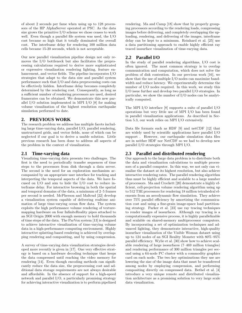
The earthquake modeling team is currently performing sim-ulations in the greater LA basin to 10 meters at the finestresolution with 100 million unstructured hexahedral finiteelements, a factor of 4000 smaller than a regular grid wouldrequire. These include simulations of the 1994 Northridgemainshock to 1 Hz resolution, the highest resolution ob-tained to date. Despite the large degree of irregularity ofthe meshes, the codes are highly efficient: close to 90% par-allel efficiency is regularly obtained in scaling up from 1to 2048 processors on the HP/Compaq AlphaServer-basedparallel system at the Pittsburgh Supercomputing Center.Node performance is also excellent for an unstructured meshcode, permitting sustained throughputs of nearly one ter-aflop per second on 2048 processors. A typical simulationrequires 25,000 time steps to simulate 40 seconds of groundshaking, and requires wall-clock time on the order of severalhours, depending on the material damping model used, sizeof the region considered, number of processors (between 512and 2048), and output statistics required. Figure 1 displayseight selected time steps from the simulation rendered usingour visualization system.

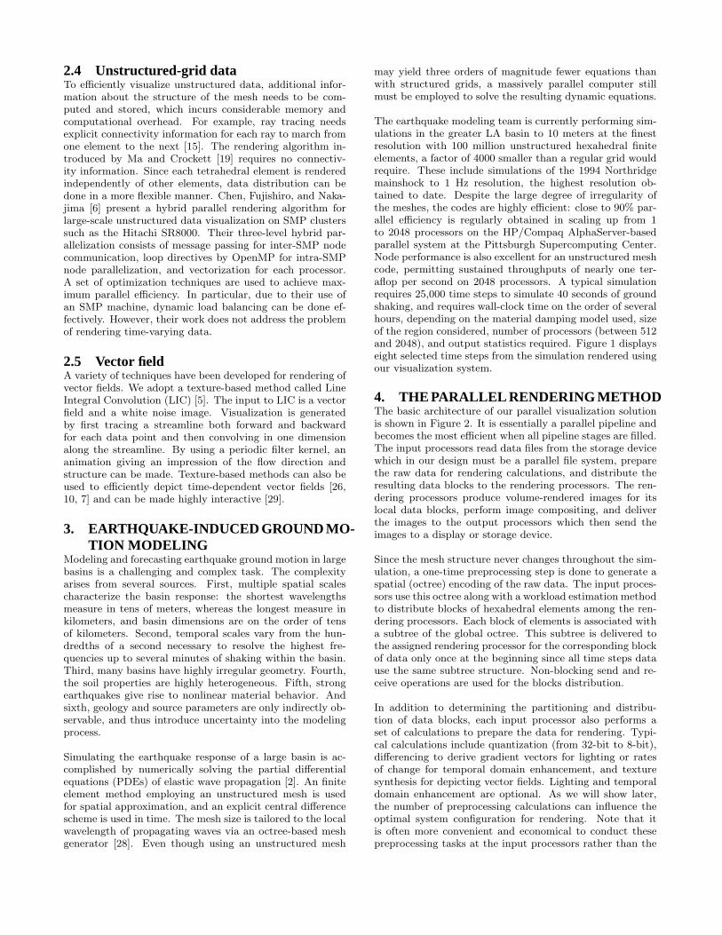
4. THE PARALLEL RENDERING METHODThe basic architecture of our parallel visualization solutionis shown in Figure 2. It is essentially a parallel pipeline andbecomes the most efficient when all pipeline stages are filled.The input processors read data files from the storage devicewhich in our design must be a parallel file system, preparethe raw data for rendering calculations, and distribute theresulting data blocks to the rendering processors. The ren-dering processors produce volume-rendered images for itslocal data blocks, perform image compositing, and deliverthe images to the output processors which then send theimages to a display or storage device.

Since the mesh structure never changes throughout the sim-ulation, a one-time preprocessing step is done to generate aspatial (octree) encoding of the raw data. The input proces-sors use this octree along with a workload estimation methodto distribute blocks of hexahedral elements among the ren-dering processors. Each block of elements is associated witha subtree of the global octree. This subtree is delivered tothe assigned rendering processor for the corresponding blockof data only once at the beginning since all time steps datause the same subtree structure. Non-blocking send and re-ceive operations are used for the blocks distribution.

In addition to determining the partitioning and distribu-tion of data blocks, each input processor also performs aset of calculations to prepare the data for rendering. Typi-cal calculations include quantization (from 32-bit to 8-bit),differencing to derive gradient vectors for lighting or ratesof change for temporal domain enhancement, and texturesynthesis for depicting vector fields. Lighting and temporaldomain enhancement are optional. As we will show later,the number of preprocessing calculations can influence theoptimal system configuration for rendering. Note that itis often more convenient and economical to conduct thesepreprocessing tasks at the input processors rather than the

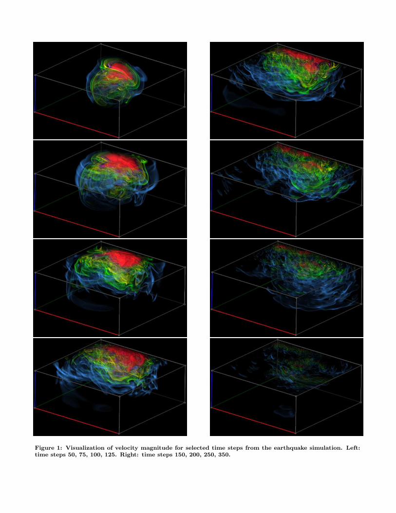
Figure 1: Visualization of velocity magnitude for selected time steps from the earthquake simulation. Left:time steps 50, 75, 100, 125. Right: time steps 150, 200, 250, 350.

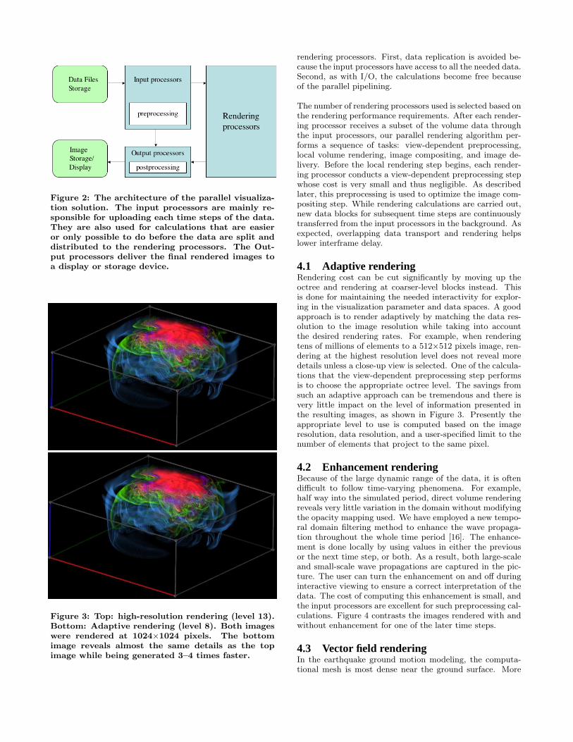
Figure 2: The architecture of the parallel visualiza-tion solution. The input processors are mainly re-sponsible for uploading each time steps of the data.They are also used for calculations that are easieror only possible to do before the data are split anddistributed to the rendering processors. The Out-put processors deliver the final rendered images toa display or storage device.

Figure 3: Top: high-resolution rendering (level 13).Bottom: Adaptive rendering (level 8). Both imageswere rendered at 1024×1024 pixels. The bottomimage reveals almost the same details as the topimage while being generated 3–4 times faster.

rendering processors. First, data replication is avoided be-cause the input processors have access to all the needed data.Second, as with I/O, the calculations become free becauseof the parallel pipelining.

The number of rendering processors used is selected based onthe rendering performance requirements. After each render-ing processor receives a subset of the volume data throughthe input processors, our parallel rendering algorithm per-forms a sequence of tasks: view-dependent preprocessing,local volume rendering, image compositing, and image de-livery. Before the local rendering step begins, each render-ing processor conducts a view-dependent preprocessing stepwhose cost is very small and thus negligible. As describedlater, this preprocessing is used to optimize the image com-positing step. While rendering calculations are carried out,new data blocks for subsequent time steps are continuouslytransferred from the input processors in the background. Asexpected, overlapping data transport and rendering helpslower interframe delay.

4.1 Adaptive renderingRendering cost can be cut significantly by moving up theoctree and rendering at coarser-level blocks instead. Thisis done for maintaining the needed interactivity for explor-ing in the visualization parameter and data spaces. A goodapproach is to render adaptively by matching the data res-olution to the image resolution while taking into accountthe desired rendering rates. For example, when renderingtens of millions of elements to a 512×512 pixels image, ren-dering at the highest resolution level does not reveal moredetails unless a close-up view is selected. One of the calcula-tions that the view-dependent preprocessing step performsis to choose the appropriate octree level. The savings fromsuch an adaptive approach can be tremendous and there isvery little impact on the level of information presented inthe resulting images, as shown in Figure 3. Presently theappropriate level to use is computed based on the imageresolution, data resolution, and a user-specified limit to thenumber of elements that project to the same pixel.

4.2 Enhancement renderingBecause of the large dynamic range of the data, it is oftendifficult to follow time-varying phenomena. For example,half way into the simulated period, direct volume renderingreveals very little variation in the domain without modifyingthe opacity mapping used. We have employed a new tempo-ral domain filtering method to enhance the wave propaga-tion throughout the whole time period [16]. The enhance-ment is done locally by using values in either the previousor the next time step, or both. As a result, both large-scaleand small-scale wave propagations are captured in the pic-ture. The user can turn the enhancement on and off duringinteractive viewing to ensure a correct interpretation of thedata. The cost of computing this enhancement is small, andthe input processors are excellent for such preprocessing cal-culations. Figure 4 contrasts the images rendered with andwithout enhancement for one of the later time steps.

4.3 Vector field renderingIn the earthquake ground motion modeling, the computa-tional mesh is most dense near the ground surface. More

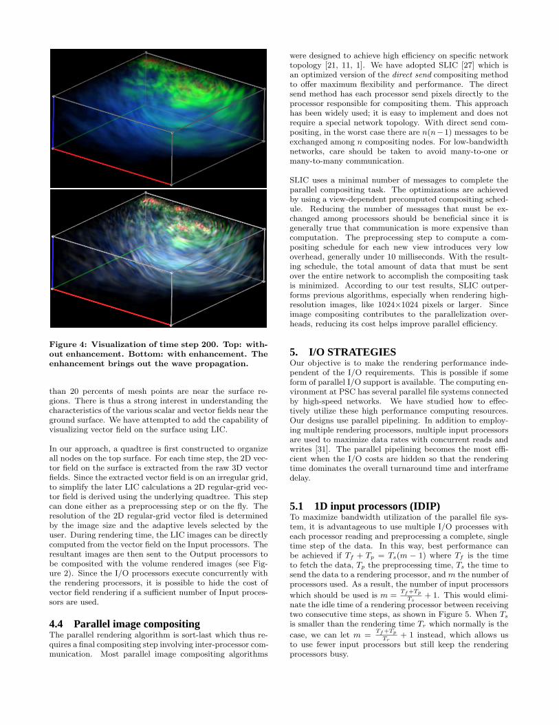
Figure 4: Visualization of time step 200. Top: with-out enhancement. Bottom: with enhancement. Theenhancement brings out the wave propagation.

than 20 percents of mesh points are near the surface re-gions. There is thus a strong interest in understanding thecharacteristics of the various scalar and vector fields near theground surface. We have attempted to add the capability ofvisualizing vector field on the surface using LIC.

In our approach, a quadtree is first constructed to organizeall nodes on the top surface. For each time step, the 2D vec-tor field on the surface is extracted from the raw 3D vectorfields. Since the extracted vector field is on an irregular grid,to simplify the later LIC calculations a 2D regular-grid vec-tor field is derived using the underlying quadtree. This stepcan done either as a preprocessing step or on the fly. Theresolution of the 2D regular-grid vector filed is determinedby the image size and the adaptive levels selected by theuser. During rendering time, the LIC images can be directlycomputed from the vector field on the Input processors. Theresultant images are then sent to the Output processors tobe composited with the volume rendered images (see Fig-ure 2). Since the I/O processors execute concurrently withthe rendering processors, it is possible to hide the cost ofvector field rendering if a sufficient number of Input proces-sors are used.

4.4 Parallel image compositingThe parallel rendering algorithm is sort-last which thus re-quires a final compositing step involving inter-processor com-munication. Most parallel image compositing algorithms

were designed to achieve high efficiency on specific networktopology [21, 11, 1]. We have adopted SLIC [27] which isan optimized version of the direct send compositing methodto offer maximum flexibility and performance. The directsend method has each processor send pixels directly to theprocessor responsible for compositing them. This approachhas been widely used; it is easy to implement and does notrequire a special network topology. With direct send com-positing, in the worst case there are n(n−1) messages to beexchanged among n compositing nodes. For low-bandwidthnetworks, care should be taken to avoid many-to-one ormany-to-many communication.

SLIC uses a minimal number of messages to complete theparallel compositing task. The optimizations are achievedby using a view-dependent precomputed compositing sched-ule. Reducing the number of messages that must be ex-changed among processors should be beneficial since it isgenerally true that communication is more expensive thancomputation. The preprocessing step to compute a com-positing schedule for each new view introduces very lowoverhead, generally under 10 milliseconds. With the result-ing schedule, the total amount of data that must be sentover the entire network to accomplish the compositing taskis minimized. According to our test results, SLIC outper-forms previous algorithms, especially when rendering high-resolution images, like 1024×1024 pixels or larger. Sinceimage compositing contributes to the parallelization over-heads, reducing its cost helps improve parallel efficiency.

5. I/O STRATEGIESOur objective is to make the rendering performance inde-pendent of the I/O requirements. This is possible if someform of parallel I/O support is available. The computing en-vironment at PSC has several parallel file systems connectedby high-speed networks. We have studied how to effec-tively utilize these high performance computing resources.Our designs use parallel pipelining. In addition to employ-ing multiple rendering processors, multiple input processorsare used to maximize data rates with concurrent reads andwrites [31]. The parallel pipelining becomes the most effi-cient when the I/O costs are hidden so that the renderingtime dominates the overall turnaround time and interframedelay.

5.1 1D input processors (IDIP)To maximize bandwidth utilization of the parallel file sys-tem, it is advantageous to use multiple I/O processes witheach processor reading and preprocessing a complete, singletime step of the data. In this way, best performance canbe achieved if Tf + Tp = Ts(m − 1) where Tf is the timeto fetch the data, Tp the preprocessing time, Ts the time tosend the data to a rendering processor, and m the number ofprocessors used. As a result, the number of input processors

which should be used is m =Tf +Tp

Ts+ 1. This would elimi-

nate the idle time of a rendering processor between receivingtwo consecutive time steps, as shown in Figure 5. When Ts

is smaller than the rendering time Tr which normally is the

case, we can let m =Tf +Tp

Tr+ 1 instead, which allows us

to use fewer input processors but still keep the renderingprocessors busy.

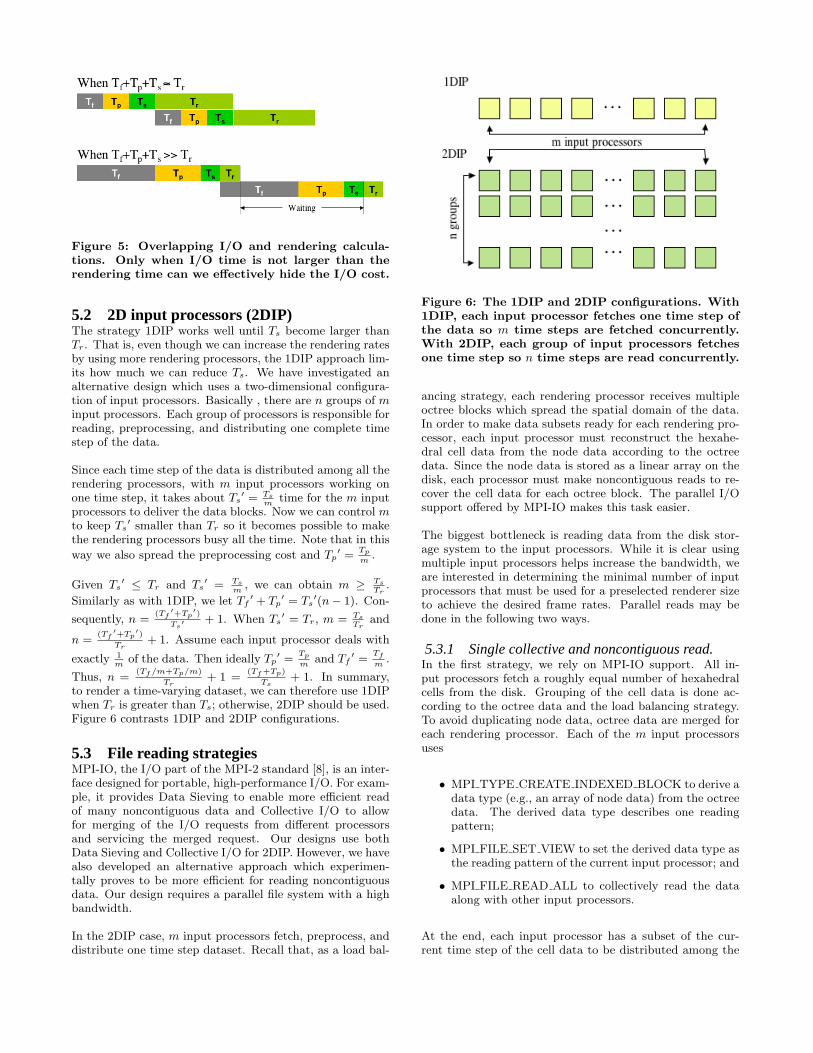
Figure 5: Overlapping I/O and rendering calcula-tions. Only when I/O time is not larger than therendering time can we effectively hide the I/O cost.

5.2 2D input processors (2DIP)The strategy 1DIP works well until Ts become larger thanTr. That is, even though we can increase the rendering ratesby using more rendering processors, the 1DIP approach lim-its how much we can reduce Ts. We have investigated analternative design which uses a two-dimensional configura-tion of input processors. Basically , there are n groups of minput processors. Each group of processors is responsible forreading, preprocessing, and distributing one complete timestep of the data.

Since each time step of the data is distributed among all therendering processors, with m input processors working onone time step, it takes about Ts

′ = Tsm

time for the m inputprocessors to deliver the data blocks. Now we can control mto keep Ts

′ smaller than Tr so it becomes possible to makethe rendering processors busy all the time. Note that in this

way we also spread the preprocessing cost and Tp′ =

Tp

m.

Given Ts′ ≤ Tr and Ts

′ = Tsm

, we can obtain m ≥ TsTr

.

Similarly as with 1DIP, we let Tf′ + Tp

′ = Ts′(n− 1). Con-

sequently, n =(Tf

′+Tp′)

Ts′ + 1. When Ts

′ = Tr, m = TsTr

and

n =(Tf

′+Tp′)

Tr+ 1. Assume each input processor deals with

exactly 1m

of the data. Then ideally Tp′ =

Tp

mand Tf

′ =Tf

m.

Thus, n =(Tf /m+Tp/m)

Tr+ 1 =

(Tf +Tp)

Ts+ 1. In summary,

to render a time-varying dataset, we can therefore use 1DIPwhen Tr is greater than Ts; otherwise, 2DIP should be used.Figure 6 contrasts 1DIP and 2DIP configurations.

5.3 File reading strategiesMPI-IO, the I/O part of the MPI-2 standard [8], is an inter-face designed for portable, high-performance I/O. For exam-ple, it provides Data Sieving to enable more efficient readof many noncontiguous data and Collective I/O to allowfor merging of the I/O requests from different processorsand servicing the merged request. Our designs use bothData Sieving and Collective I/O for 2DIP. However, we havealso developed an alternative approach which experimen-tally proves to be more efficient for reading noncontiguousdata. Our design requires a parallel file system with a highbandwidth.

In the 2DIP case, m input processors fetch, preprocess, anddistribute one time step dataset. Recall that, as a load bal-

Figure 6: The 1DIP and 2DIP configurations. With1DIP, each input processor fetches one time step ofthe data so m time steps are fetched concurrently.With 2DIP, each group of input processors fetchesone time step so n time steps are read concurrently.

ancing strategy, each rendering processor receives multipleoctree blocks which spread the spatial domain of the data.In order to make data subsets ready for each rendering pro-cessor, each input processor must reconstruct the hexahe-dral cell data from the node data according to the octreedata. Since the node data is stored as a linear array on thedisk, each processor must make noncontiguous reads to re-cover the cell data for each octree block. The parallel I/Osupport offered by MPI-IO makes this task easier.

The biggest bottleneck is reading data from the disk stor-age system to the input processors. While it is clear usingmultiple input processors helps increase the bandwidth, weare interested in determining the minimal number of inputprocessors that must be used for a preselected renderer sizeto achieve the desired frame rates. Parallel reads may bedone in the following two ways.

5.3.1 Single collective and noncontiguous read.In the first strategy, we rely on MPI-IO support. All in-put processors fetch a roughly equal number of hexahedralcells from the disk. Grouping of the cell data is done ac-cording to the octree data and the load balancing strategy.To avoid duplicating node data, octree data are merged foreach rendering processor. Each of the m input processorsuses

• MPI TYPE CREATE INDEXED BLOCK to derive adata type (e.g., an array of node data) from the octreedata. The derived data type describes one readingpattern;

• MPI FILE SET VIEW to set the derived data type asthe reading pattern of the current input processor; and

• MPI FILE READ ALL to collectively read the dataalong with other input processors.

At the end, each input processor has a subset of the cur-rent time step of the cell data to be distributed among the

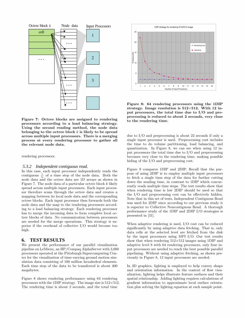
Figure 7: Octree blocks are assigned to renderingprocessors according to a load balancing strategy.Using the second reading method, the node databelonging to the octree block k is likely to be spreadacross multiple input processors. There is a mergingprocess at every rendering processor to gather allthe relevant node data.

rendering processors.

5.3.2 Independent contiguous read.In this case, each input processor independently reads thecontiguous 1

mof a time step of the node data. Both the

node data and the octree data are 1D arrays as shown inFigure 7. The node data of a particular octree block k likelyspread across multiple input processors. Each input proces-sor therefore scans through the octree data and creates amapping between its local node data and the correspondingoctree blocks. Each input processor then forwards both thenode data and the map to the rendering processors accord-ing to a load balancing strategy. Each rendering processorhas to merge the incoming data to form complete local oc-tree blocks of data. No communication between processorsare needed for the merge operations. This strategy is su-perior if the overhead of collective I/O would become toohigh.

6. TEST RESULTSWe present the performance of our parallel visualizationpipeline on LeMieux, an HP/Compaq AlphaServer with 3,000processors operated at the Pittsburgh Supercomputing Cen-ter for the visualization of time-varying ground motion sim-ulation data consisting of 100 million hexahedral elements.Each time step of the data to be transferred is about 400megabytes.

Figure 8 shows rendering performance using 64 renderingprocessors with the 1DIP strategy. The image size is 512×512.The rendering time is about 2 seconds, and the total time

1DIP strategy for rendering 512X512 image

0

5

10

15

20

25

1 2 3 4 5 6 7 8 9 10 11 12 13 14 15 16

Number of Input Processors

Tim

e(se

cond

s)

Rendering time

Total time

Figure 8: 64 rendering processors using the 1DIPstrategy. Image resolution is 512×512. With 12 in-put processors, the total time due to I/O and pre-processing is reduced to about 2 seconds, very closeto the rendering time.

due to I/O and preprocessing is about 22 seconds if only asingle input processor is used. Preprocessing cost includesthe time to do volume partitioning, load balancing, andquantization. In Figure 8, we can see when using 12 in-put processors the total time due to I/O and preprocessingbecomes very close to the rendering time, making possiblehiding of the I/O and preprocessing cost.

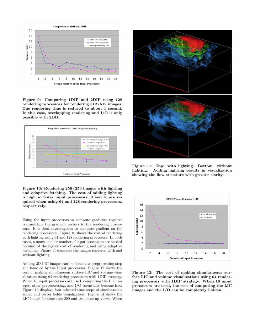
Figure 9 compares 1DIP and 2DIP. Recall that the pur-pose of using 2DIP is to employ multiple input processorsto fetch a single time step of the data for further cuttingdown the sending time, in contrast to 1DIP which concur-rently reads multiple time steps. The test results show thatwhen rendering time is low 2DIP should be used so thatthe I/O and preprocessing cost can be effectively hidden.Note that in this set of tests, Independent Contiguous Readwas used for 2DIP since according to our previous study itis superior to Collective Noncontiguous Read. A thoroughperformance study of the 1DIP and 2DIP I/O strategies ispresented in [31].

When adaptive rendering is used, I/O cost can be reducedsignificantly by using adaptive data fetching. That is, onlydata cells at the selected level are fetched from the diskby the input processors using MPI I/O. Our test resultsshow that when rendering 512×512 images using 1DIP andadaptive level 8 with 64 rendering processors, only four in-put processors are needed to reach the best possible parallelpipelining. Without using adaptive fetching, as shown pre-viously in Figure 8, 12 input processors are needed.

In 3D graphics, lighting is employed to help convey shapeand orientation information. In the context of flow visu-alization, lighting helps illustrate feature surfaces and theirspatial relationship. Adding lighting requires calculations ofgradient information to approximate local surface orienta-tion plus solving the lighting equation at each sample point.

Comparison of 1DIP and 2DIP

0

2

4

6

8

10

12

14

16

1 2 4 6 8 10 12 14 16 18 20 22

Group number of the Input Processors

Tim

e(se

con

ds)

Total time using IDIP

Total time using 2DIP

Average rendering time

Figure 9: Comparing 1DIP and 2DIP using 128rendering processors for rendering 512×512 images.The rendering time is reduced to about 1 second.In this case, overlapping rendering and I/O is onlypossible with 2DIP.

Using 1DIP to render 512x512 image with lighting

Number of Input Processors

Tim

e (s

eco

nd

s)

Rendering t ime using 128 PEs

T otal t ime using 128 PEs

Rendering t ime using 64 PEs

T otal t ime using 64 PEs

Figure 10: Rendering 256×256 images with lightingand adaptive fetching. The cost of adding lightingis high so fewer input processors, 3 and 4, are re-quired when using 64 and 128 rendering processors,respectively.

Using the input processors to compute gradients requirestransmitting the gradient vectors to the rendering proces-sors. It is thus advantageous to compute gradient on therendering processors. Figure 10 shows the cost of renderingwith lighting using 64 and 128 rendering processors. In bothcases, a much smaller number of input processors are neededbecause of the higher cost of rendering and using adaptivefeatching. Figure 11 contrasts the images rendered with andwithout lighting.

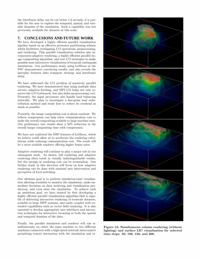
Adding 2D LIC images can be done as a preprocessing stepand handled by the Input processors. Figure 12 shows thecost of making simultaneous surface LIC and volume visu-alization using 64 rendering processors with 1DIP strategy.When 16 input processors are used, computing the LIC im-ages, other preprocessing, and I/O essentially become free.Figure 13 displays four selected time steps of simultaneousscalar and vector fields visualization. Figure 14 shows theLIC image for time step 200 and two close-up views. When

Figure 11: Top: with lighting. Bottom: withoutlighting. Adding lighting results in visualizationshowing the flow structure with greater clarity.

512*512 Volume Rendering + LIC

0

2

4

6

8

10

12

14

16

2 4 6 8 10 12 14 16 18

Number of Input Processors

Tim

e(se

con

ds)

Rendering time

Total time

Figure 12: The cost of making simultaneous sur-face LIC and volume visualizations using 64 render-ing processors with 1DIP strategy. When 16 inputprocessors are used, the cost of computing the LICimages and the I/O can be completely hidden.

the interframe delay can be cut below 1-2 seconds, it is pos-sible for the user to explore the temporal, spatial, and vari-able domains of the simulation. Such a capability was notpreviously available for datasets at this scale.

7. CONCLUSIONS AND FUTURE WORKWe have developed a highly efficient parallel visualizationpipeline based on an effective processor partitioning schemewhich facilitates overlapping I/O operations, preprocessing,and rendering. This parallel visualization solution also in-corporates adaptive rendering, a highly efficient parallel im-age compositing algorithm, and new I/O strategies to makepossible near-interactive visualization of terascale earthquakesimulations. Our performance study using LeMieux at thePSC demonstrates convincing results, and also reveals theinterplay between data transport strategy and interframedelay.

We have addressed the I/O problem of massively parallelrendering. We have demonstrated that using multiple dataservers, adaptive fetching, and MPI I/O helps not only re-moves the I/O bottleneck, but also hides preprocessing cost.Presently, the input processors also handle load balancingstatically. We plan to investigate a fine-grain load redis-tribution method and study how to reduce its overhead asmuch as possible.

Presently, the image compositing cost is about constant. Webelieve compression can help lower communication cost tomake the overall compositing scalable to large machine sizes.Our preliminary test results show a 50% reduction in theoverall image compositing time with compression.

We have not exploited the SMP features of LeMieux, whichwe believe could allow us to accelerate the rendering calcu-lations while reducing communication cost. The result willbe a more scalable renderer offering higher frame rates.

Adaptive rendering will continue to play a major role in oursubsequent work. As shown, full rendering and adaptiverendering often result in visually indistinguishable results,but the savings in rendering cost can be tremendous. Ourfurther study in this direction will focus on how adaptiverendering can be done with minimal user intervention andperception of level switching.

Our ultimate goal is to perform simulation-time visualiza-tion allowing scientists to monitor the simulation, make im-mediate decisions on data archiving and visualization pro-duction, and even steer the simulation. To achieve suchan ambitious goal, we have started by first developing ahighly efficient parallel visualization algorithm that is capa-ble of delivering interactive rendering of terascale datasets,scalable to large MPP systems, and easily coupled with ex-tended capabilities such as vector field rendering. It is alsoessential to develop appropriate user interfaces and interac-tion techniques for interactive browsing in both the spatialand temporal domains of the data.

Finally, the parallel simulation and renderer will run si-multaneously on either the same machine or two differentmachines connected with a high-speed network interconnectpermitting remote interaction with the simulation and vi-

Figure 13: Simultaneous volume rendering (withoutlighting) and surface LIC visualization for selectedtime steps: 50, 100, 150, and 200.

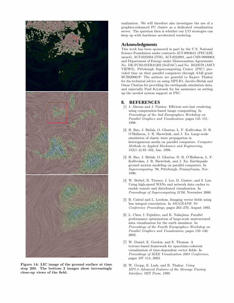
Figure 14: LIC image of the ground surface at timestep 200. The bottom 2 images show increasinglyclose-up views of the field.

sualization. We will therefore also investigate the use of agraphics-enhanced PC cluster as a dedicated visualizationserver. The question then is whether our I/O strategies cankeep up with hardware accelerated rendering.

AcknowledgmentsThis work has been sponsored in part by the U.S. NationalScience Foundation under contracts ACI 9983641 (PECASEaward), ACI 0325934 (ITR), ACI 0222991, and CMS-9980063;and Department of Energy under Memorandum AgreementsNo. DE-FC02-01ER41202 (SciDAC) and No. B523578 (ASCIVIEWS). Pittsburgh Supercomputing Center (PSC) pro-vided time on their parallel computers through AAB grantBCS020001P. The authors are grateful to Rajeev Thakurfor his technical advice on using MPI-IO, Jacobo Bielak andOmar Chattas for providing the earthquake simulation data,and especially Paul Krystosek for his assistance on settingup the needed system support at PSC.

8. REFERENCES[1] J. Ahrens and J. Painter. Efficient sort-last rendering

using compression-based image compositing. InProceedings of the 2nd Eurographics Workshop onParallel Graphics and Visualization, pages 145–151,1998.

[2] H. Bao, J. Bielak, O. Ghattas, L. F. Kallivokas, D. R.O’Hallaron, J. R. Shewchuk, and J. Xu. Large-scalesimulation of elastic wave propagation inheterogeneous media on parallel computers. ComputerMethods in Applied Mechanics and Engineering,152(1–2):85–102, Jan. 1998.

[3] H. Bao, J. Bielak, O. Ghattas, D. R. O’Hallaron, L. F.Kallivokas, J. R. Shewchuk, and J. Xu. Earthquakeground motion modeling on parallel computers. InSupercomputing ’96, Pittsburgh, Pennsylvania, Nov.1996.

[4] W. Bethel, B. Tierney, J. Lee, D. Gunter, and S. Lau.Using high-speed WANs and network data caches toenable remote and distributed visualization. InProceedings of Supercomputing 2C00, November 2000.

[5] B. Cabral and L. Leedom. Imaging vector fields usingline integral convolution. In SIGGRAPH ’93Conference Proceedings, pages 263–270, August 1993.

[6] L. Chen, I. Fujishiro, and K. Nakajima. Parallelperformance optimization of large-scale unstructureddata visualization for the earth simulator. InProceedings of the Fourth Eurographics Workshop onParallel Graphics and Visualization, pages 133–140,2002.

[7] W. Daniel, E. Gordon, and E. Thomas. Atexture-based framework for spacetime-coherentvisualization of time-dependent vector fields. InProceedings of IEEE Visualization 2003 Conference,pages 107–114, 2003.

[8] W. Gropp, E. Lusk, and R. Thakur. UsingMPI-2–Advanced Features of the Message PassingInterface. MIT Press, 1999.

[9] HDF5 home page, the national center forsupercomputing applications.http://hdf.ncsa.uiuc.edu/HDF5.

[10] B. Jobard, G. Erlebacher, and M. Hussaini.Lagrangian-eulerian advection for unsteady flowvisualization. In Proceedings of IEEE Visualization2001 Conference, pages 53–60, 2001.

[11] T.-Y. Lee, C. S. Raghavendra, and J. B. Nicholas.Image composition schemes for sort-last polygonrendering on 2d mesh multicomputers. IEEETransactions on Visualization and ComputerGraphics, 2(3):202–217, 1996.

[12] J. Li, W.-K. Liao, A. Choudhary, R. Ross, R. Thakur,W. Gropp, R. Latham, A. Siegel, B. Gallagher, andM. Zingale. Parallel netCDF: A high-performancescientific I/O interface. In Proceedings ofSupercomputing 2003 Conference, November 2003.

[13] P. Li, S. Whitman, R. Mendoza, and J. Tsiao. ParVox– a parallel spaltting volume rendering system fordistributed visualization. In Proceedings of 1997Symposium on Parallel Rendering, pages 7–14, 1997.

[14] E. Lum, K.-L. Ma, and J. Clyne. A hardware-assistedscalable solution for interactive volume rendering oftime-varying data. IEEE Transactions onVisualization and Computer Graphics, 8(3):286–301,2002.

[15] K.-L. Ma. Parallel volume ray-casting forunstructured-grid data on distributed-memoryarchitectures. In Proceedings of the Parallel Rendering’95 Symposium, pages 23–30, 1995. Atlanta, Georgia,October 30-31.

[16] K.-L. Ma. Visualizing large-scale earthquakesimulations. In Proceedings of the Supercomputing2003 Conference, 2003.

[17] K.-L. Ma. Visualizing time-varying volume data.IEEE Computing in Science & Engineering,5(2):34–42, 2003.

[18] K.-L. Ma and D. Camp. High performancevisualization of time-varying volume data over awide-area network. In Proceedings of Supercomputing2000 Conference, November 2000.

[19] K.-L. Ma and T. Crockett. A scalable parallelcell-projection volume rendering algorithm forthree-dimensional unstructured data. In Proceedings of1997 Symposium on Parallel Rendering, pages 95–104,1997.

[20] K.-L. Ma and T. Crockett. Parallel visualization oflarge-scale aerodynamics calculations: A case study onthe cray t3e. In Proceedings of 1999 IEEE ParallelVisualization and Graphics Symposium, pages 15–20,1999.

[21] K.-L. Ma, J. S. Painter, C. Hansen, and M. Krogh.Parallel Volume Rendering Using Binary-SwapCompositing. IEEE Computer Graphics Applications,14(4):59–67, July 1994.

[22] A. McPherson and M. Maltrud. Poptex: Interactiveocean model visualization using texture mappinghardware. In Proceedings of the Visualization ’98Conference, pages 471–474, October 18-23 1998.

[23] S. Parker, M. Parker, Y. Livnat, P. Sloan, andC. Hansen. Interactive Ray Tracing for VolumeVisualization. IEEE Transactions on Visualization andComputer Graphics, 5(3):1–13, July-September 1999.

[24] The Quake project, Carnegie Mellon University andSan Diego State University.http://www.cs.cmu.edu/˜quake.

[25] E. Reinhard, C. Hansen, and S. Parker. Interactiveray tracing of time-varying data. In Proceedings of the4th Eurographics Workshop on Parallel Graphihcs andVisualization, 2002.

[26] H.-W. Shen and D. Kao. A new line integralconvolution algorithm for visualizing time-varying flowfields. IEEE Transactions on Visualization andComputer Graphics, 4(2), 1998.

[27] A. Stompel, K.-L. Ma, E. Lum, J. Ahrens, andJ. Patchett. SLIC: scheduled linear image compositingfor parallel volume rendering. In Proceedings of IEEESympoisum on Parallel and Large-Data Visualizationand Graphics (to appear), October 2003.

[28] T. Tu, D. O’Hallaron, and J. Lopez. Etree: Adatabase-oriented method for generating large octreemeshes. In Proceedings of the Eleventh InternationalMeshing Roundtable, pages 127–138, September 2002.

[29] J. van Wijk. Image based flow visualization. InProceedings of SIGGRAPH 2002 Conference, 2002.

[30] B. Wylie, C. Pavlakos, V. Lewis, and K. Moreland.Scalable rendering on PC clusters. IEEE ComputerGraphics and Applications, 21(4):62–70, July/August2001.

[31] H. Yu, K.-L. Ma, and J. Welling. I/O strategy forparallel rendering of large time-varying volume data.In Proceedings of 2004 Parallel Graphics andVisualization Symposium (to appear), 2004.