A parallel algorithm for Lagrange interpolation on thecube-connected cycles

H. Sarbazi-Azada, M. Ould-Khaouab,* , L.M. Mackenziea

aDepartment of Computing Science, University of Glasgow, Glasgow G12 8QQ, UKbDepartment of Computer Science, University of Strathclyde, Glasgow G1 1XH, UK

Received 12 May 1999; received in revised form 21 December 1999; accepted 17 January 2000

Abstract

This paper introduces a parallel algorithm for computing anN � n2n point Lagrange interpolation on ann-dimensional cube-connectedcycles (CCCn). The algorithm consists of three phases: initialisation, main and final. While there is no computation in the initialisation phase,the main phase is composed ofn2n21 steps, each consisting of four multiplications, four subtractions and one communication operation, andan additional step including one division and one multiplication. The final phase is carried out in two sub-phases. There aredn=2e steps in thefirst sub-phase, each including two additions and one communication, followed by the second sub-phase which comprisesn steps eachconsisting of one addition and two communication operations.q 2000 Elsevier Science B.V. All rights reserved.

Keywords: Interconnection networks; Cube-connected cycles; Parallel algorithms; Lagrange interpolation

1. Introduction

The cube-connected cycle (or CCC for short) has beenintroduced by Preparata and Vuillamin [14] as a practicalsubstitute for the well-known hypercube. The CCC over-comes the scalability problem, e.g. increased node degreeas the network size scales up, associated with the hypercubetopology, while maintaining most of its desirable properties,such as rich and powerful connectivity and good routingcapabilities [11]. The CCC also exhibits a strong structuralrelationship to other network topologies such as deBrujin,shuffle-exchange and butterfly networks [1,7,11]. Severalimportant aspects, including mapping and VLSI layout ofthe CCC have been widely studied in the past[3,5,6,10,12,13].

Interpolation techniques are of great importance innumerical analysis since they are widely used in a varietyof science and engineering domains where numerical solu-tion is the only way to predict the value of a tabulatedfunction for new input data. Many methods have beenproposed of which Lagrange interpolation is one of thebest known techniques.Lagrangeinterpolation [16] for agiven set of points (x0, y0), (x2, y2),…,(xN21, yN21) and the

valuex is carried out via the formula

f �x� �XN 2 1

i�0

yiLi�x� �1�

where the termLi is called a Lagrange polynomial, and isgiven by:

Li�x� �YN 2 1

j�0

�x 2 xj��xi 2 xj� ; j ± i �2�

When the number of points,N, is very large, long compu-tation time and large storage capacity may be required tocarry out the above computation. To overcome this, severalauthors have proposed parallel implementations for theLagrange interpolation. For instance, Capello et al. [4]have described an algorithm using 2N 2 1 steps onN/2processors where each step, after implementation, requirestwo subtractions, two multiplications and one division.Goertzel [8] has introduced a parallel algorithm suitablefor a tree topology withN processors, augmented withring connections. The algorithm requiresN/2 1 O(log N)steps, each composed of two subtractions and four multi-plications which is about two times faster than the algorithmintroduced in [4]. However, it requires an asymmetric topol-ogy with a node degree of five. More recently, a parallelalgorithm has been discussed in [15] which uses ak-ary n-cube, consisting ofkn

=2 1 O�kn� steps, each with four

Microprocessors and Microsystems 24 (2000) 135–140

0141-9331/00/$ - see front matterq 2000 Elsevier Science B.V. All rights reserved.PII: S0141-9331(00)00066-1

www.elsevier.nl/locate/micpro

* Corresponding author. Tel.:1 44-141-5483098; fax: 1 44-141-5525330.

E-mail address:mohamed@cs.strath.ac.uk (M. Ould-Khaoua).

multiplications and subtractions, for anN � kn node inter-polation. It has the advantage of employing a popularsymmetric network, i.e. ak-ary n-cube whose node degreeis 2n.

This paper proposes a parallel algorithm for computingLagrange interpolation on the CCC. The algorithm relies onall-to-all broadcast communication at some stages duringcomputation, as will be discussed later. This is achievedby using a gossiping algorithm on a ring embedded in thehost CCC using all of its nodes. The proposed algorithm isslightly faster than the algorithm introduced in Ref. [15] butslightly slower than that in Ref. [8]. However, the CCC has asymmetric topology with a fixed node degree of 3. More-over, it can be simulated easily on a hypercube where eachcycle in then-dimensional CCC is mapped to a node in ann-dimensional hypercube.

The rest of the paper is organized as follows. Section 2gives a definition for the CCC. Section 3 introduces theproposed parallel algorithm and discusses it in details.Finally Section 4 concludes this paper.

2. The cube-connected cycles

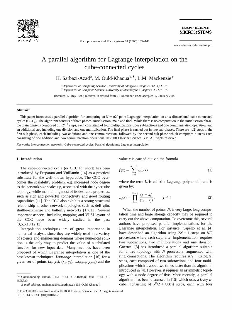
The n-dimensional cube-connected cycle, CCCn, isconstructed from the binaryn-cube (also calledn-dimen-sional hypercube) by replacing each of its nodes with acycle of n nodes. Theith dimension edge incident to anode of the hypercube is then connected to theith node ofthe corresponding cycle of the CCC. Therefore, the resultingnetwork hasN � n2n nodes each with degree 3. Each nodecan be represented by a pair (w, r) wherer �1 # r # n� is theposition of the node within its cycle andw� w1w2…wn

(any n-bit binary string) is the label of the node in thehypercube that corresponds to the cycle. Then two nodes(w, r) and (w0, r 0) are linked by an edge in the CCCn if andonly if either

1. w� w0 andr 2 r 0 � ^1 modn; or2. r � r 0 andw differs from w0 in precisely therth bit, i.e.

wj � w0j�1 # j # n; j ± r�; andwr ± w0r :

Edges of the first type are calledcycle edges, while edges of

the second type are referred to ashypercube edges[5,11].Fig. 1 shows two- and three-dimensional cube-connectedcycles, CCC2 and CCC3, respectively.

3. The parallel algorithm

The proposed parallel algorithm computesy� f �x� on aCCCn given the set of points (x0, y0), (x1, y1),…,(xN21, yN21)and valuex, whereN � n2n

: The computation is carried outin three phases:initialisation, main and final phase. First,the set of points to be interpolated are allocated to the nodes,one point for each node. Then, the Lagrange polynomials,Li�x�; �0 # i , N�; are computed. Finally the sum of theterms Li�x� × yi ; �0 # i , N�; is calculated to obtain thefinal result,y� f �x�; according to Eq. (1).

Before describing these phases in more details, thissection introduces some of the notation which will beused in the development of the algorithm. Let each proces-sing node have four registers,R1, R2, R3 and R4. In eachnode, registersR1 and R2 store the terms required forcomputing a Lagrange polynomial and registersR3 andR4

are used to implement an all-to-all broadcast algorithm in aring embedded in the host network, CCCn, during the mainphase. We shall use notationPw,r to indicate therth node inthe ring with addressw of the corresponding hypercube. TheregisterRk �1 # k # 4� in Pw,r is denoted asPw,r (Rk) ingeneral andP�t�w;r �Rk� after stept. Each step may involve aset of communication and computation operations. Symbol‘ ( ’ denotes a communication operation between the twoadjacent nodes.

3.1. The initialisation phase

In this phase, the value ofx, point �x�r21�2n1w; y�r21�2n1w�and address valuesNext_r[w,r], and Previous_r[w,r] arefirstly given to the processorPw;r ; �0 # w , 2n 2 1;1 # r # n�. As will be discussed in the next section,Next_r[w,r] and Previous_r[w,r] will be used in the mainphase to address the next and the previous node of thecurrent node in the order that form a ring of processorsembedded in the employed CCC. Then, registersR1–R4 ofeach processor are set to their initial values by the followinginstruction sequence:

P�0�w;r �R1�← 1;

P�0�w;r �R2�← 1;

P�0�w;r �R3�← x�r21�2n1w;

P�0�w;r �R4�← x�r21�2n1w:

The initialisation phase can be implemented in a pipelinefashion, requiring only communication and no computation.

H. Sarbazi-Azad et al. / Microprocessors and Microsystems 24 (2000) 135–140136

(a) (b)

00

01 11

101

2

2

1

1 1

2

000

001

010

011 111

110

100

101 2

1

1

1

1

1 1

11

2

2

2

2

2

2

2

2

3

3

3

33

3

3

Fig. 1. Examples of CCC: (a) three-dimensional cube-connected cycles,CCC3; (b) two-dimensional cube-connected cycles, CCC2.

3.2. The main phase

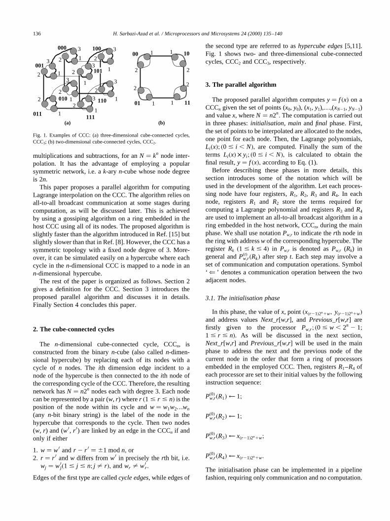
Examining the communication pattern inherent in theinterpolation algorithm reveals that each nodePw;r ; �0 #w , 2n; 1 # r # n� needs at some point to broadcast thevaluex�r21�2n1w to all the other nodes in the network. Thisall-to-all broadcast operation is best performed according tothe ring topology. As this ring should contain all nodes ofthe used CCC, the algorithm uses, in the main phase, aHamiltonianembedded in the host network CCCn; a Hamil-tonian ring (also called Hamiltonian cycle or circuit) is aring embedded in the host network including all its nodes[11]. To achieve this, we use the algorithm shown in Fig. 2.This algorithm is based on the proof that appeared in Ref.[11] which proceeds with inductive reasoning onn. It proves

that there is a Hamiltonian cycle in a CCCn having supposedthat there is a Hamiltonian cycle embedded in a CCCn22.Induction base aren� 2 and n� 3 that the embeddedHamiltonian cycle for these cases have been illustrated inFig. 1 (with bold links). The algorithm (shown in Fig. 2)embeds a Hamiltonian ring in a CCCn and initializes two-dimensional arraysNext_r andPrevious_rwhich indicate,respectively, ther-address of the nodes after and beforePw,r

in the embedded Hamiltonian cycle. As the initialisationphase uses these arrays, they should have been set to theirproper values before starting the initialisation phase. Duringthe initialisation phase each nodePw;r ; �0 # w , 2n; 1 #r # n� receives its appropriate data, including addressvaluesNext_r[w,r] and Previous_r[w,r] and stores addressvalues in two local variable (preferably registers) called

H. Sarbazi-Azad et al. / Microprocessors and Microsystems 24 (2000) 135–140 137

Algorithm Hamiltonian_cycle_embedding_in_CCCn;Input: Degree of the desired cube-connected cycles, nOutput: Ring embedded in the CCCn(Ring)and arrays Next_r[0..2n-1,1..n] and Previous_r[0..2n-1,1..n];

BEGIN

If (n is even) then{ Ring← Hamiltonian ring embedded in CCC2;

C← 2; /* current degree=2*/};

Else{ Ring← Hamiltonian ring embedded in CCC3;

C← 3; /* current degree=3*/ };

while (C<n) do{

for w← 0 to 2C-1 do Replace link <(w,1),(w,C)> with the path <(w,1), (w,C+2), (w, C+1), (w, C)> in Ring;

Ring00 ← Ring;Ring01 ← Ring;Ring10 ← Ring;Ring11 ← Ring;

Remove link <(00…000, C+2),(00…000, C+1)> in Ring00 , <(00…001, C+2),(00…001, C+1)> in Ring01 , <(00…010, C+2),(00…010, C+1)> in Ring10 and <(00…011, C+2),(00…011, C+1)> in Ring11;

Establish a link between nodes (00…000,C+2) of Ring00 and (00…001,C+2) in Ring01 , a link between nodes (00…001,C+1) of Ring01 and (00…011,C+1) in Ring11 , a link between nodes (00…011,C+2) of Ring11 and (00…010,C+2) in Ring10 and a link between nodes (00…010,C+1) of Ring10 and (00…000,C+1) in Ring00 ;

Copy the big cycle composed of Ring00 , Ring01 , Ring10 ,and Ring11 into Ring;

C← C+2;};

for w← 0 to 2n-1 dofor r ← 1 to n do

{ Next_r[w,r] ← r-address of the node located after node (w,r) in Ring;Previous_r[w,r] ← r-address of the node located before node (w,r) in Ring;

};

END;

e

Fig. 2. The algorithm for embedding a Hamiltonian cycle into the CCCn.

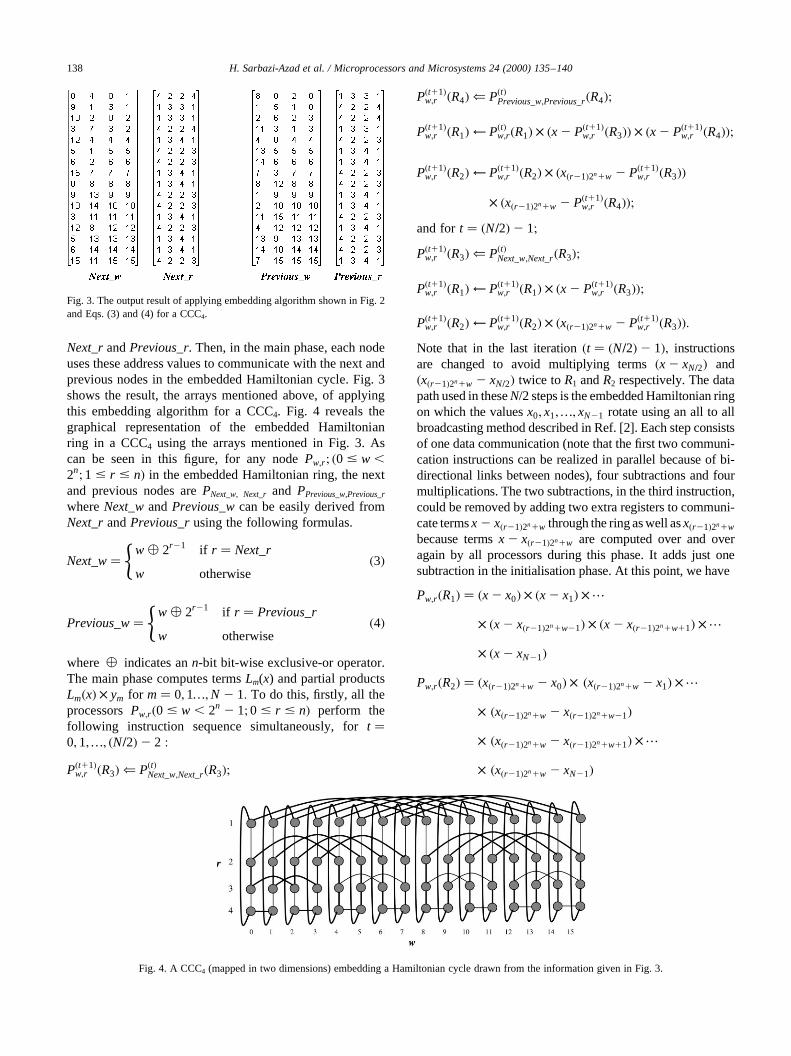
Next_randPrevious_r. Then, in the main phase, each nodeuses these address values to communicate with the next andprevious nodes in the embedded Hamiltonian cycle. Fig. 3shows the result, the arrays mentioned above, of applyingthis embedding algorithm for a CCC4. Fig. 4 reveals thegraphical representation of the embedded Hamiltonianring in a CCC4 using the arrays mentioned in Fig. 3. Ascan be seen in this figure, for any nodePw;r ; �0 # w ,2n; 1 # r # n� in the embedded Hamiltonian ring, the nextand previous nodes arePNext_w, Next_r and PPrevious_w,Previous_r

whereNext_wandPrevious_wcan be easily derived fromNext_randPrevious_rusing the following formulas.

Next_w� w % 2r21 if r � Next_r

w otherwise

(�3�

Previous_w� w % 2r21 if r � Previous_r

w otherwise

(�4�

where % indicates ann-bit bit-wise exclusive-or operator.The main phase computes termsLm(x) and partial productsLm�x� × ym for m� 0;1…;N 2 1: To do this, firstly, all theprocessorsPw;r �0 # w , 2n 2 1;0 # r # n� perform thefollowing instruction sequence simultaneously, fort �0; 1;…; �N=2�2 2 :

P�t11�w;r �R3� ( P�t�Next_w;Next_r�R3�;

P�t11�w;r �R4� ( P�t�Previous_w;Previous_r�R4�;

P�t11�w;r �R1�← P�t�w;r �R1� × �x 2 P�t11�

w;r �R3�� × �x 2 P�t11�w;r �R4��;

P�t11�w;r �R2�← P�t11�

w;r �R2� × �x�r21�2n1w 2 P�t11�w;r �R3��

× �x�r21�2n1w 2 P�t11�w;r �R4��;

and fort � �N=2�2 1;

P�t11�w;r �R3� ( P�t�Next_w;Next_r�R3�;

P�t11�w;r �R1�← P�t11�

w;r �R1� × �x 2 P�t11�w;r �R3��;

P�t11�w;r �R2�← P�t11�

w;r �R2� × �x�r21�2n1w 2 P�t11�w;r �R3��:

Note that in the last iteration�t � �N=2�2 1�; instructionsare changed to avoid multiplying terms�x 2 xN=2� and�x�r21�2n1w 2 xN=2� twice toR1 andR2 respectively. The datapath used in theseN/2 steps is the embedded Hamiltonian ringon which the valuesx0; x1;…; xN21 rotate using an all to allbroadcasting method described in Ref. [2]. Each step consistsof one data communication (note that the first two communi-cation instructions can be realized in parallel because of bi-directional links between nodes), four subtractions and fourmultiplications. The two subtractions, in the third instruction,could be removed by adding two extra registers to communi-cate termsx 2 x�r21�2n1w through the ring as well asx�r21�2n1w

because termsx 2 x�r21�2n1w are computed over and overagain by all processors during this phase. It adds just onesubtraction in the initialisation phase. At this point, we have

Pw;r �R1� � �x 2 x0� × �x 2 x1� × …

× �x 2 x�r21�2n1w21� × �x 2 x�r21�2n1w11� × …

× �x 2 xN21�Pw;r �R2� � �x�r21�2n1w 2 x0� × �x�r21�2n1w 2 x1� × …

× �x�r21�2n1w 2 x�r21�2n1w21�× �x�r21�2n1w 2 x�r21�2n1w11� × …

× �x�r21�2n1w 2 xN21�

H. Sarbazi-Azad et al. / Microprocessors and Microsystems 24 (2000) 135–140138

Fig. 3. The output result of applying embedding algorithm shown in Fig. 2and Eqs. (3) and (4) for a CCC4.

Fig. 4. A CCC4 (mapped in two dimensions) embedding a Hamiltonian cycle drawn from the information given in Fig. 3.

As the last step in this phase, all the processors execute thefollowing instruction:

P��N=2�11�w;r �R1�← P�N=2�

w;r �R1�P�N=2�

w;r �R2�× y�r21�2n1w

Therefore, at the end of this phase, we havePw;r �R1� �L�r21�2n1w × y�r21�2n1w: In the main phase, each processorperformsN/2 data communications (because of bi-directionallinks providing the ability of simultaneous communicationbetween two adjacent nodes in both directions), 2N 1 1 multi-plications, 2N subtractions and one division.

3.3. The final phase

In this phase, the contents of registerR1 in all nodes areadded together to obtain the final result. To this end, anystandard algorithm for gossiping and accumulation in CCCcan be used (e.g. see Ref. [9]). The algorithm used in thisphase consists of two sub-phases. In the first sub-phase, thecontent of registersR1 of all nodes in any vertex ringPw;p; �0 # w , 2n 2 1�; are added together so thatPw;r �R1� �

Pni�1 Pw;r �R1�; �0 # w # 2n 2 1; 1 # r # n�:

Similar to the gossiping method for a ring used in themain phase, the gossiping process between nodes of eachrings is realized inn/2 steps (note that the each vertex ringhasn nodes), each including one communication and twoadditions.

for w� 0;1;…; 2n 2 1 in parallelfor r � 1;2;…; n in parallel

{ Pw;r �R3�← Pw;r �R1�;Pw;r �R4�← Pw;r �R1�;

};for i � 1;2;…; bn=2cfor w� 0;1;…; 2n 2 1 in parallel

for r � 1;2;…; n in parallel{ Pw;r �R3� ( Pw;�r mod n�11�R3�;

Pw;r �R4� ( Pw;�r mod n�21�R4�;Pw;r �R1�← Pw;r �R1�1 Pw;r �R3�1 Pw;r �R4�if (n is even) and �i � �N=2�2 1� thenPw;r �R3�← 0;

};

In the second sub-phase, the partial results accumulated inregistersR1 of nodes in all the rings (one node of each ring)are added together to obtain the final resulty� f �x�: It isrealized inn steps each consisting of one addition and twocommunication operations. Each step reduces the size ofproblem by one until the last step,nth step, which completethe computation having stored the final result in registerR1

of processorP0,1.

for i � 1;2;…;nfor w� 0;1;…;2n2i 2 1 in parallel{ Pw;i�R1� ( Pw;i�R1�1 Pw12n2i ;i�R1�;

Pw;�i mod n�11�R1� ( Pw;i�R1�;};

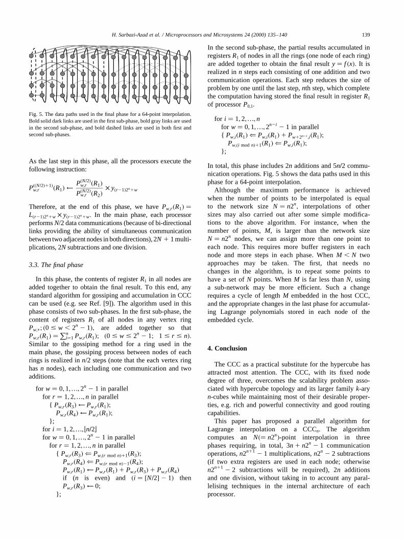
In total, this phase includes 2n additions and 5n=2 commu-nication operations. Fig. 5 shows the data paths used in thisphase for a 64-point interpolation.

Although the maximum performance is achievedwhen the number of points to be interpolated is equalto the network sizeN � n2n

; interpolations of othersizes may also carried out after some simple modifica-tions to the above algorithm. For instance, when thenumber of points,M, is larger than the network sizeN � n2n nodes, we can assign more than one point toeach node. This requires more buffer registers in eachnode and more steps in each phase. WhenM , N twoapproaches may be taken. The first, that needs nochanges in the algorithm, is to repeat some points tohave a set ofN points. WhenM is far less thanN, usinga sub-network may be more efficient. Such a changerequires a cycle of lengthM embedded in the host CCC,and the appropriate changes in the last phase for accumulat-ing Lagrange polynomials stored in each node of theembedded cycle.

4. Conclusion

The CCC as a practical substitute for the hypercube hasattracted most attention. The CCC, with its fixed nodedegree of three, overcomes the scalability problem asso-ciated with hypercube topology and its larger familyk-aryn-cubes while maintaining most of their desirable proper-ties, e.g. rich and powerful connectivity and good routingcapabilities.

This paper has proposed a parallel algorithm forLagrange interpolation on a CCCn. The algorithmcomputes an N�� n2n�-point interpolation in threephases requiring, in total, 3n 1 n2n 2 1 communicationoperations,n2n11 2 1 multiplications,n2n 2 2 subtractions(if two extra registers are used in each node; otherwisen2n11 2 2 subtractions will be required), 2n additionsand one division, without taking in to account any paral-lelising techniques in the internal architecture of eachprocessor.

H. Sarbazi-Azad et al. / Microprocessors and Microsystems 24 (2000) 135–140 139

Fig. 5. The data paths used in the final phase for a 64-point interpolation.Bold solid dark links are used in the first sub-phase, bold gray links are usedin the second sub-phase, and bold dashed links are used in both first andsecond sub-phases.

References

[1] F. Annexstein, et al., action graphs and parallel architectures, SIAM J.Comput. 19 (1990) 544–569.

[2] A. Bertsekas, Tsitsiklis, Parallel and Distributed Computation:Numerical Methods, Prentice-Hall, Englewood Cliffs, NJ, 1989.

[3] G. Calrson, et al., Interconnection networks based on generalizationsof cube-connected cycles, IEEE Trans. Computers C-34 (1985) 769–772.

[4] B. Capello, et al., computation of interpolation polynomials, ParallelComput. 45 (1990) 95–117.

[5] G. Chen, F.C.M. Lau, A tight layout of the cube-connected cycles,Proceedings of the Fourth International Conference on High Perfor-mance Computing (HiPC’97), IEEE Computer Society Press, NewYork, 1997.

[6] W.J. Dally, C.L. Seitz, Deadlock-free message routing in multipro-cessor interconnection networks, IEEE Trans. Computers C-36(1987) 547–553.

[7] R. Feldmann, W. Unger, The cube-connected cycles is a subgraph ofthe Butterfly network, Parallel Processing Lett. 2 (1992) 13–19.

[8] B. Goertzel, Lagrange interpolation on a tree of processors withring connections, , J. Parallel Distribut. Comput. 22 (1994) 321–323.

[9] J. Hromovic, et al., Dissemination of Information in interconnectionnetworks (Broadcasting and Gossiping), in: F. Hsu, D. Du, et al.(Eds.), Combinational Network Theory, Kluwer Academic,Dordrecht, 1995, pp. 125–212.

[10] R. Klasing, Improved compression of cube-connected cyclesnetworks, IEEE Trans. Parallel Distribut. Syst. 9 (1998) 803–812.

[11] F.T. Leighton, Introduction to Parallel Algorithms and Architec-tures: Arrays, Trees, Hypercubes, Morgan Kaufmann, Los Altos,CA, 1992.

[12] D. Meliksetian, C. Chen, Optimal routing algorithm and the diameterof the cube-connected cycles, IEEE Trans. Parallel Distribut Syst. 4(1993) 1172–1178.

[13] D. Meliksetian, C. Chen, Communication aspects of the cube-connected cycles, Proceedings of the International Conference onParallel Processing, 1990, pp. I-579–580.

[14] F.P. Preparata, J. Vuillemin, The cube-connected cycles: a versatilenetwork for parallel computation, CACM 24 (1981) 300–309.

[15] H. Sarbazi-Azad, M. Ould-Khaoua, L.M. Mackenzie, A parallel algo-rithm for Lagrange interpolation onkary n-cubes, Proceedings of theFourth International Conference of the Austrian Centre for ParallelComputation (ACPC’99), Salzburg, Austria, 16–18 February,Lecture Notes in Computer Science, Springer, Berlin, 1999 (pp.85–95).

[16] B. Wendroff, Theoretical Numerical Analysis, Academic Press, NewYork, 1966.

H. Sarbazi-Azad et al. / Microprocessors and Microsystems 24 (2000) 135–140140

Hamid Sarbazi-Azad was born in 1968,Ray, Tehran, Iran. He received his BScdegree in Electrical and Computer Engi-neering from the Shahid-Beheshti Univer-sity, Tehran, in 1992, and the MSc degreein Computer Engineering from the SharifUniversity of Technology, Tehran, Iran, in1994. From graduation until 1997, heworked as a research faculty member atthe National Organisation for the Evalua-tion of Education, Tehran. He is currentlypursuing his PhD study in the Department

of Computing Science at the University of Glasgow, Glasgow, UK,through a scholarship from the Ministry of Culture and Higher Educa-tion of the Islamic Republic of Iran. His research interests includeparallel computing, interconnection networks, and their performanceevaluation.

Mohamed Ould-Khaoua received hisBSc degree from the University of Algiers,Algeria, in 1986, and the MAppSci andPhD degrees in Computer Science fromthe University of Glasgow, UK, in 1990and 1994, respectively. He is currently alecturer in the Department of ComputerScience at the University of Strathclyde,Glasgow, UK. His research focuses onapplying theoretical results from stochasticprocesses and queueing theory to thequantitative study of hardware and soft-

ware architectures. His current research interests are performancemodelling/evaluation, interconnection networks, parallel architectures,parallel algorithms, and ATM networks.

Lewis M. Mackenzie graduated with aBSc in Mathematics and Natural Philo-sophy from the University of Glasgow in1980. He was awarded the PhD in 1984,also at the University of Glasgow, for hiswork in the development of multicom-puters for use in nuclear physics. He nowlectures at the Department of ComputerScience at the University of Glasgow,which he joined in 1985. His currentresearch interests include multicomputers,high-performance networks, and simulation.